AIR COMPRESSION PERFORMANCE IMPROVEMENT VIA TRAJECTORYOPTIMIZATION - EXPERIMENTAL VALIDATION

Mohsen SaadatDept. of Mechanical Engineering

University of MinnesotaMinneapolis, MN 55455

Email: saad0021@umn.edu

Anirudh SrivatsaDept. of Mechanical Engineering

University of MinnesotaMinneapolis, MN 55455

Email: sriva047@umn.edu

Perry Y. LiDept. of Mechanical Engineering

University of MinnesotaMinneapolis, MN 55455

Email: lixxx099@umn.edu

Terrence SimonDept. of Mechanical Engineering

University of MinnesotaMinneapolis, MN 55455

Email: simon002@umn.edu

ABSTRACT

In an isothermal compressed air energy storage (CAES) sys-tem, it is critical that the high pressure air compressor/expanderis both efficient and power dense. The fundamental trade-off be-tween efficiency and power density is due to limitation in heattransfer capacity during the compression/expansion process. Inour previous works, optimization of the compression/expansiontrajectory has been proposed as a means to mitigate this trade-off. Analysis and simulations have shown that the use of op-timized trajectory can increase power density significantly (2-3fold) over ad-hoc linear or sinusoidal trajectories without sac-rificing efficiency especially for high pressure ratios. This pa-per presents the first experimental validation of this approach inhigh pressure (7bar to 200bar) compression. Experiments areperformed on an instrumented liquid piston compressor. Corre-lations for the heat transfer coefficient were obtained empiricallyfrom a set of CFD simulations under different conditions. Dy-namic programming approach is used to calculate the optimalcompression trajectories by minimizing the compression time fora range of desired compression efficiencies. These compressionprofiles (as function of compression time) are then tracked in aliquid piston air compressor testbed using a combination of feed-

forward and feedback control strategy. Compared to ad-hoc con-stant flow rate trajectories, the optimal trajectories double thepower density at 80% efficiency or improve the thermal efficiencyby 5% over a range of power densities.

1 INTRODUCTIONCompressed air energy storage is a potential solution for

mitigating the variable and unpredictable nature of renewable

energies like wind or solar. Fig. 1 shows the Open Accumu-

lator Isothermal Compressed Air Energy Storage (OA-ICAES)

system introduced in [1] and [2] for storing excess energy for

wind turbine. A key component of this system is the high pres-

sure air compressor/expander unit which is responsible for the

transformation between mechanical work and stored energy in

the form of compressed air. As such it must be efficient as well

as powerful enough to handle the power requirement.

For a system without any thermal storage (except the envi-

ronment at the ambient temperature), the most efficient process

is the isothermal compression/expansion process at the ambient

temperature. However, an ideal isothermal process takes infi-

nite amount of time and hence absorbs/produces no power since

Proceedings of the ASME 2016 Dynamic Systems and Control Conference DSCC2016

October 12-14, 2016, Minneapolis, Minnesota, USA

DSCC2016-9825

1 Copyright © 2016 by ASME

power is work divided by time. This is because the heat transfer

with the environment becomes vanishingly small as the temper-

ature differential with the heat source/sink approaches zero. As

process time decreases, power increases but the process deviates

more and more from the isothermal process leading to reduced

efficiency. This illustrates the trade-off between efficiency and

power density where power density refers to the power normal-

ized by the compressor/expander volume.

This efficiency-power density trade-off is mediated by heat

transfer so that increasing heat transfer capability per unit vol-

ume will improve the trade-off. One approach is to inject tiny

water droplets during the compression/expansion process [3, 4]

since the droplets present large surface area and heat capacity for

heat transfer. This is especially useful for the low pressure stage

compressor/expander. A second approach is to use a liquid pis-

ton compressor/expander that is filled with porous media. Since

liquid can flow through the porous media, the liquid piston can

compress the air above it while the porous media increases heat

transfer surface area and heat capacitance. Analysis and experi-

ment have shown that use of porous media with 70-80% porosity

can increase the power density by an order of magnitude without

sacrificing efficiency [5–7]. The liquid piston approach is espe-

cially attractive for the high pressure stage since the liquid also

forms an effective seal for the air being compressed and serves

to eliminate residual dead volume.

Water Pump/Motor

(F2)

t

Air

Oil

Water

WP

Waterr r

erertete

atatW

aW

aWWWW

Oil Water

Storage Vessel (Accumulator)

(E)

Wind Turbine

(A)

Generator (G)

Electrical Grid Air Compressor/

Expander (F1)

Hydraulic Pump/Motor

(C)

(D)

(B)

FIGURE 1: Schematic of the Open Accumulator Isothermal

Compressed Air Energy Storage (OA-ICAES) system [1, 2]

Yet another approach is to optimize and control the rate of

compression/expansion. Optimizing the compression/expansion

trajectory allows the process to better match the heat transfer ca-

pability. Analytical and numerical studies have shown that use

of optimal compression/expansion trajectories can significantly

increase power density (by 2 to 3 fold for high pressure) over ad-

hoc linear or sinusoidal trajectories [8–11] for both simple and

complex heat transfer models. However, experimental validation

of the efficacy of this approach has only been done for low pres-

sure (1bar to 10bar) [12] where the benefit is relatively minor.

Since the benefit of optimal trajectory is more important for high

pressure, the goal of this paper is to experimentally validate this

concept in high pressure (7bar to 200bar) operation.

The rest of the paper is organized as follows. Section 2

presents the experimental setup. The heat transfer coefficient

correlation obtained empirically from extensive CFD exper-

iments is presented in Section 3. Calibration of the critical

volume measurement is presented in Section 4. Design and

control of the optimal trajectories are given in Section 5.

Experimental results are given in Section 6. Concluding remarks

are given in Section 7.

2 Experimental SetupThe schematic and picture of the liquid piston air compres-

sor experiment setup are shown in Figs. 2 and 3. The setup

was designed to study the compression/expansion processes dur-

ing single shot experiments. In this system, a double-acting hy-

draulic cylinder (4) is coupled with a single-acting water cylin-

der (5) so that extension of the hydraulic piston will cause the

water piston to be retracted and vice versa. The hydraulic cylin-

der is connected to a hydraulic power supply (at 200bar) via a

solenoid-actuated servo-valve. This valve is used to control the

oil flow rate to the hydraulic cylinder and to regulate its exten-

sion speed at a desired value. A magnetic incremental encoder is

connected to the tandem rod (between the hydraulic cylinder and

water cylinder) in order to measure the displacement of water

piston, which will be used to calculate the volume of water dis-

placed into the compression chamber. The compression chamber

is a vertical cylinder made of stainless steel and is connected to

the water cylinder via a combination of hoses and ball valves.

Retracting the water piston causes water to be pushed into the

compression chamber and raises the water column level inside

it. This will compress the air inside the compression chamber.

A pressure transducer is located at the top of compression cham-

ber to measure the air pressure during compression process. A

transparent plastic side tube is used to estimate the initial level

of liquid column in the compression chamber and calculate the

initial air volume in it. By knowing the amount of water that

is displaced into the compression chamber (from water cylin-

der), it would be possible to estimate the air volume inside the

compression chamber during the compression process. A com-

bination of ball valves and a single poppet valve (mounted on

top of the compression chamber) are used to control the filling

of the chamber with fresh air. While the liquid piston air com-

pressor is considered for compressing air from 7bar to 200bar,

a conventional solid-piston air compressor is used to compress

air from ambient pressure to 7bar. By opening the poppet valve,

the compression chamber is filled with fresh air at 7bar provided

by the solid-piston air compressor. After the chamber is filled

2 Copyright © 2016 by ASME

FIGURE 2: Detailed schematic of liquid piston air compressor experimental setup [6, 7]

FIGURE 3: Liquid piston air compressor; Left: water hydraulic cylinder and connections; Right: compression chamber [6, 7]

with air, the poppet valve closes and the system becomes ready

for compression process. By regulating the flow rate through the

hydraulic servo-valve, it would be possible to control the exten-

sion speed of hydraulic piston which in turn defines the retraction

speed of water piston and consequently the water flow rate into

the compression chamber. Therefore, a previously defined flow

rate (as a function of compression time) can be tracked using an

appropriate closed-loop controller. More details and information

regarding this experimental facility can be found in [6] where the

same setup was used to study the effect of porous media. In this

paper, the effect of optimal trajectories will be studied without

using porous media.

3 Heat Transfer ModelingComputing the optimal compression trajectory is sensitive

to the model used for heat transfer prediction between air under

3 Copyright © 2016 by ASME

compression and compression chamber walls. Either underesti-

mating or overestimating the heat transfer between air and heat

exchanger material (in our case, the chamber’s walls since porous

media is not used) results in a wrong optimal compression pro-

file, which in turn reduces the improvement of power density (for

a fixed thermal efficiency). Therefore, the first step in calculating

the optimal compression profile is to find a reasonably accurate

heat transfer model for the chamber.

Assuming lumped properties for air (i.e. zero-dimensional

temperature and pressure), the heat transfer between air and its

surrounding environment (described by Q) can be written as:

Q(t) = hA(Tair −Twall) (1)

where h is the convective heat transfer coefficient, A is the avail-

able heat transfer area, Tair is the air temperature and Twall is the

wall temperature that is assumed to remain constant during the

compression process (Twall = 295K). While calculating the total

heat transfer area is easy (since it’s only a function of air vol-

ume at any time), evaluating heat transfer coefficient is relatively

complex since it is an instantaneous function of air properties,

piston speed and chamber geometry. To find this dependency, a

series of numerical simulations is performed in COMSOL Mul-

tiphysics software to investigate the correlation between convec-

tive heat transfer coefficient and air properties, piston speed and

chamber geometry.

While there are many parameters that affect the heat trans-

fer coefficient, a comprehensive study is performed by changing

some parameters while keeping the rest of them constant, in or-

der to study their effect on heat transfer coefficient. It should be

emphasized that such a flexibility is only available in numerical

analysis since the experimental investigation for revealing the de-

pendency of heat transfer to different parameters is very difficult

and time consuming. According to the comprehensive numeri-

cal analysis that is done in COMSOL, a correlation between h,

aspect ratio of air column L/D (ratio between length of air col-

umn L and its diameter D), piston speed U , heat conductivity k,

density ρ and viscosity μ of air is suggested as:

Y = c1X2 + c2X + c3 (2)

where X and Y are:

X =ρμ

Ua(μ

k

)b(3)

Y =hk

(LD

)d

(4)

To find the best combination for a,b and d, an optimization

problem is defined and solved. Here, we are looking for the best

set of parameters that results in minimum difference between the

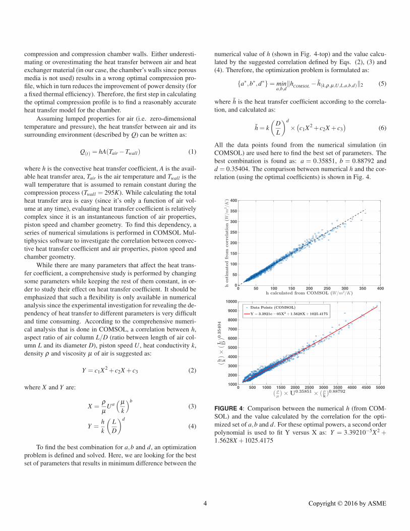
numerical value of h (shown in Fig. 4-top) and the value calcu-

lated by the suggested correlation defined by Eqs. (2), (3) and

(4). Therefore, the optimization problem is formulated as:

{a∗,b∗,d∗}= mina,b,d

‖hCOMSOL − h(k,ρ,μ,U,L,a,b,d)‖2 (5)

where h is the heat transfer coefficient according to the correla-

tion, and calculated as:

h = k(

DL

)d

× (c1X2 + c2X + c3

)(6)

All the data points found from the numerical simulation (in

COMSOL) are used here to find the best set of parameters. The

best combination is found as: a = 0.35851, b = 0.88792 and

d = 0.35404. The comparison between numerical h and the cor-

relation (using the optimal coefficients) is shown in Fig. 4.

h calculated from COMSOL (W/m2/K)0 50 100 150 200 250 300 350 400

hestim

ated

from

correlation

(W/m

2/K

)

0

50

100

150

200

250

300

350

400

( ρμ)×U0.35851 × (μk )

0.887920 500 1000 1500 2000 2500 3000 3500 4000 4500 5000

(h k)×

(L D)0

.35404

1000

2000

3000

4000

5000

6000

7000

8000

9000

10000Data Points (COMSOL)

Y = 3.3921e− 05X2 + 1.5628X+ 1025.4175

FIGURE 4: Comparison between the numerical h (from COM-

SOL) and the value calculated by the correlation for the opti-

mized set of a,b and d. For these optimal powers, a second order

polynomial is used to fit Y versus X as: Y = 3.39210−5X2 +1.5628X +1025.4175

4 Copyright © 2016 by ASME

4 Estimation of Air Volume in the CompressionChamberDirect measurement of the air volume in the compression

chamber is not available in the experimental setup. Instead, air

volume is estimated from the initial air volume and the change

in water volume. Because water is slightly compressible and the

components such as hoses expand, the change in water volume

in the chamber consists of the volume of water injected and the

volume change due to pressure. Thus, the air volume in the com-

pression chamber can be expressed as:

V(t) =V0 −V Displaced(t) +VC

(P) (7)

where V0 is the initial volume of air in the chamber at the begin-

ning of compression (i.e. t = 0), VC is the pressure dependent

volume adjustment due to water compressibility and system ex-

pansion, and V Displaced is the volume of water pushed into the

compression chamber from the water cylinder. It is important to

consider VC since it can account for 30% of the volume at the

end of compression.

The pressure dependent volume adjustment term VC is ob-

tained by filling the chamber completely with water and com-

pressing it. The result is shown in Fig. 5. VC has a larger slope

at lower pressures which is due to soft components such as hoses

and entrained air in the water. At higher pressures (> 10bar), it

has a constant slope which is slightly greater than that due pure

water compressibility.

Pressure (bar)0 20 40 60 80 100 120 140 160 180 200

System

Expansion

(cc)

0

10

20

30

40

50

60Raw DataFiltered DataPure Water Compressibility (for comparision)

FIGURE 5: Summation of water compression and system expan-

sion (such as hoses, cylinder and connections) due to pressure

rise. Pure water compressibility is also plotted for comparison

(bulk modulus of 2.2GPa is assumed).

The displaced water volume term V Displaced should ideally

be proportional to the movement of the water hydraulic cylinder

as reflected by the linear magnetic encoder measurement C. In

order to account for any slight nonlinearity, a quadratic relation

is used. Eq. (7) becomes:

V(t) =V0 −K1C(t)−K2C2(t) +VC

(P) (8)

FIGURE 6: Sample test shows the method for evaluating the con-

stant parameters in air volume estimation. Air compression is

from t = 60s to t = 100s. The liquid column is maintained at its

position from t = 100s until the air pressure reaches its steady-

state value. This means that air is cooled down to ambient tem-

perature. To achieve more isothermal points, the liquid column is

retracted by small steps to let air pressure drops and then stayed

there for a while until air pressure reaches its new steady-state

value.

To account for any small changes in each experiment, the

parameters V0, K1 and K2 are calibrated for each experiment. To

do this, at the end of each experiment, the air in the chamber is

allowed to return to ambient temperature at successive volumes

(the liquid piston is withdrawn in each step). A sample pressure

trace in shown Fig. 6. Notice the step decreases in pressures

at the end of the experiment. Assuming ideal gas behavior (the

same approach can be done with real gas model), air volume and

pressure after the air has returned to ambient temperature (i.e. at

the end of each step) must satisfy:

T1 = T2 = . . .Tn (9)

⇒ P1V1 = P2V2 = . . .= PmVm (10)

where Vi, i = 1, . . .m can be expressed using (8). The coefficients

V0, K1 and K2 are then optimized to minimize the relative error

in (10), specifically,

{V ∗0 ,K

∗1 ,K

∗2}= min

V0,K1,K2

VAR(

Pi(V0 −K1Ci −K2C2i +VC

(Pi)))(11)

5 Copyright © 2016 by ASME

where VAR denotes the variance of the m air pressure and vol-

ume products. The approach described above is used for each

compression test since the initial air volume for each run can be

slightly different than the other tests. For the sample case shown

in Fig. 6 these parameters are found as follows:

V0 = 2.292×10−3m3

K1 = 1.196×10−7m3/count,

K2 = 2.316×10−14m3/count2

5 Design and Implementation of the Optimal Com-pression TrajectoriesThe heat transfer correlation found based on COMSOL sim-

ulations is used to calculate a series of optimal compression tra-

jectories for the given chamber geometry and desired initial and

final pressures. The optimization problem is formulated such that

the compression time is the cost function while the compression

efficiency is an equality constraint that needs to be satisfied. The

flow rate must also be below the pressure dependent flow capa-

bility of the system. Dynamic Programming (DP) approach is

then used to solve the optimal control problem [11].

A combined feedback and feedforward controller is used to

track the optimal flow trajectory in the compression chamber.

According to (8), the air volume rate of change can be calculated

as:

V =−F(t) =−K1C−2K2CC+dVC

dPP (12)

An open loop calibration test is first performed on the system

(in terms of different voltages on hydraulic servo-valve) to eval-

uate the required command signal for a given flow rate at a given

pressure. This map is found as shown in Fig. 7. By inverting

the results, it would be possible to find the required servo valve

voltage for a desired piston speed at a given pressure. This map

is used in the feedforward controller. The feedback part of the

controller is simply a PI controller on air volume error (differ-

ence between the actual air volume and the desired air volume

calculated by time integral of optimal flow rate). The controller

block diagram used for this experiment is shown in Fig. 8.

6 Experimental ResultsThe experimental results of applying the optimal trajectories

are shown in Fig. 9. The optimal compression profile starts with

the maximum available flow rate (Qmax = 800cc/s), which is fol-

lowed by a much lower flow that continues for nearly the rest of

the compression process. A short fast compression concludes the

process and achieves the final desired pressure (200bar) at the

end. Such fast-slow-fast trajectories are consistent with optimal

trajectories from our previous studies [8–11].

0 0 0 0

1 1 1 1

2 2 22

33

33

3

44

4

4

4

55

55

5

Air Pressure (bar)50 100 150 200

WaterPisto

nFlow

Rate

(cc/s)

100

200

300

400

500

600

700

800

Serv

oValveCommand

(voltage)

0

0.5

1

1.5

2

2.5

3

3.5

4

4.5

5

FIGURE 7: Calibration of hydraulic servo valve that is used in

feedforward controller

F*(t) Fig. 5 F

- - +dt∫ d∫

t

V0air

++ PI-Controller Co

++ Plant PFig 5F

- -++

Pair

Vair

Vair

U

Ufb

Uff

Pair

FIGURE 8: Control strategy for tracking the optimal flow rate

In order to evaluate the performance improvement achieved

by applying the optimal compression trajectories, a series of con-

stant flow rate compressions is also conducted on the experi-

mental setup. Result of this experiment is shown in Fig. 10.

The closed loop controller maintains the flow rate at the desired

value, while the flow rate drops at the end of compression process

due to limited flow rate at high pressures. To compare the per-

formance of optimal and non-optimal (i.e. constant flow) com-

pression trajectories, the compression efficiencies are calculated

from [11, 12]:

η =Stored Energy

Input Work=

EW

(13)

E =−∫ V iso

f

V0

PisodV iso +Pisof V iso

f −P0V0 (14)

W =−∫ Vf

V0

PdV +PfVf −P0V0 (15)

6 Copyright © 2016 by ASME

Higher Effic

iency

Higher Efficiency

Higher Efficiency

FIGURE 9: Optimal compression flow rate results; Top: optimal

flow rate versus time ratio (t/tend where tend is the total compres-

sion time); Middle: air pressure versus air volume ratio (V/V0

where V0 is the initial air volume); Bottom: air pressure versus

compression time

note that the integration for E in Eq. (14) is taken over an isother-

mal compression process1 which starts at (P0,V0) and ends at

(V isof ,Piso

f ) (see [2,11] for more details). The compression power

density is defined as the ratio between the storage power and the

total volume of compression chamber:

Power Density = PD =E

tendV0(16)

Compression efficiency and power density for each test are cal-

culated based on Eqs. (13), (14), (15) and (16). Results in

1Real gas model is used instead of ideal gas model for better accuracy at high

pressures [13]

Higher Efficiency

Higher Efficiency

Higher Efficiency

FIGURE 10: Constant flow rate compression results; Top: flow

rate versus time ratio (t/tend where tend is the total compression

time); Middle: air pressure versus air volume ratio (V/V0 where

V0 is the initial air volume); Bottom: air pressure versus com-

pression time

terms of efficiency versus compression time and efficiency ver-

sus power density are shown in Fig. 11. In general, the opti-

mal compression flow rate results in a smaller compression time,

therefore a larger storage power density for the same thermal ef-

ficiency. According to the experimental results, for the given

chamber geometry and initial and final pressures, this improve-

ment can be as high as 100% for thermal efficiencies around 80%

(from 55kW/m3 to 120kW/m3). Hence, a compression chamber

that uses constant flow rate to compress air can be downsized to

its half size and maintains its performance (compression power

and thermal efficiency) if it uses the optimal compression rate to

compress air. The performance improvement can be also inter-

preted as a higher thermal efficiency for the same storage power

7 Copyright © 2016 by ASME

density. According to the results, this raise in thermal efficiency

can be as high as 5% for storage powers around 100kW/m3 (from

75% to 80%).

100% improvement in power density

5% improvement in efficiency

FIGURE 11: Comparison between the optimal flow rate and

non-optimal (constant) flow rate compression; Top: thermal effi-

ciency versus compression time; Bottom: thermal efficiency ver-

sus storage power density.

7 ConclusionsPrevious theoretical and numerical studies have shown that

applying optimal compression/expansion trajectory is an effec-

tive approach to improve the performance of an air compres-

sor/expander machine by optimizing the trade-off between ef-

ficiency and power density. It is also known that an accurate heat

transfer model for the compression/expansion chamber is critical

in order to design optimal flow profiles and improve the system

performance. In this work, a systematic approach was used to

find a correlation that models the convective heat transfer coef-

ficient between air and compression chamber wall. This corre-

lation is found by numerical simulation performed in COMSOL.

This correlation is then used to calculate the optimal compression

trajectories that minimize compression time for a given (desired)

compression efficiency. Dynamic programming approach was

applied to determine a family of optimal compression flow pro-

files. The optimal performance of the system is then compared

with non-optimal performance that is generated by using ad-hoc

compression trajectories (here constant flow rate compression).

According to the results, a 5% thermal efficiency improvement

is achievable at 100kW/m3 storage power density. Likewise, the

storage power can be doubled at 80% efficiency if the constant

flow rate is replaced by the corresponding optimal compression

trajectory.

AcknowledgementsThis work is supported by the National Science Foundation

under grant ENG/EFRI-1038294.

REFERENCES[1] P. Y. Li, E. Loth, T. W. Simon, J. D. Van de Ven, and Stephen

E. Crane, “Compressed Air Energy Storage for Offshore Wind

Turbines,” International Fluid Power Exhibition (IFPE), Las

Vegas, NV, March 2011.

[2] M. Saadat and P. Y. Li, “Modeling and Control of an Open

Accumulator Compressed Air Energy Storage (CAES) Sys-

tem for Wind Turbines, ” Applied Energy, Vol. 137, pp. 603-

616, January 2015.

[3] C. Qin, E. Loth, P. Li, T. Simon, and J. D. Van de Ven,

“Spray-cooling concept for Wind-Based Compressed Air En-

ergy Storage,” Journal of Renewable and Sustainable Energy,

Vol. 6, 2014.

[4] M. Saadat, F. Shirazi and P. Y. Li, “Optimal Trajectories of

Water Spray for a Liquid Piston Air Compressor,” ASME Sum-mer Heat Transfer Conference, HT2013-17611, Minneapolis,

MN, July 2013.

[5] C. Zhang, M. Saadat, P. Y. Li and T.W. Simon, “Heat Trans-

fer in a Long, Thin Tube Section of an Air Compressor: An

Empirical Correlation from CFD and a Thermodynamic Mod-

eling,” ASME IMECE, Paper #86673, Houston TX, November

2012.

[6] J. Wieberdink, “Increasing Efficiency & Power Density Of a

Liquid Piston Air Compressor / Expander With Porous Media

Heat Transfer Elements, ” M.S. Thesis, U. of Minnesota, 2014.

[7] Bo Yan et. al.,“Experimental Study of Heat Transfer En-

hancement in a Liquid Piston Compressor/Expander Using

Porous Media Inserts, ” Applied Energy, Vol. 154, pp. 40-50,

September 2015.

[8] C. Sancken and P. Y. Li, “Optimal Efficiency-Power Rela-

tionship for an Air Motor-Compressor in an Energy Storage

and Regeneration System, ” Proceedings of the ASME 2009Dynamic Systems and Control Conference, DSCC2009/Bath

Symposium PTMC, Hollywood, 2009.

[9] A. T. Rice and P. Y. Li, “Optimal Efficiency-Power Trade-

off for an Air Motor/Compressor with Volume Varying Heat

8 Copyright © 2016 by ASME

Transfer Capability, ” ASME DSCC 2011/Bath Symposium onPTMC, Arlington, VA, October 2011.

[10] M. Saadat, P. Y. Li and T. W. Simon, “Optimal Trajectories

for a Liquid Piston Compressor/Expander in a Compressed

Air Energy Storage System with Consideration of Heat Trans-

fer and Friction, ” Americal Control Conference, Montreal,

Canada, June 2012.

[11] M. Saadat and P. Y. Li, “Combined Optimal Design and

Control of a Near Isothermal Liquid Piston Air Compres-

sor/Expander for a Compressed Air Energy Storage (CAES)

System for Wind Turbines, ” ASME DSCC, Columbus, USA,

October 2015.

[12] F. A. Shirazi, M. Saadat, B. Yan, P. Y. Li and T. W. Si-

mon,“Iterative Optimal Control of a Near Isothermal Liquid

Piston Air Compressor in a Compressed Air Energy Storage

System, ” American Control Conference, Washington, DC,

June 2013.

[13] Lemmon, E.W., Jacobsen, R.T., Penoncello, S.G., Friend,

D.G., “Thermodynamic properties of air and mixtures of ni-

trogen, argon, and oxygen from 60 to 2000 K at pressures

to 2000 MPa, ” Journal of Physical and Chemical ReferenceData, Vol. 29, pp. 331-385, 2000.

9 Copyright © 2016 by ASME