939
Airpak 3.0 User’s Guide May 2, 2007
| Date post: | 24-Dec-2015 |
| Category: |
Documents |
| Upload: | gowtham-mech |
| View: | 443 times |
| Download: | 18 times |

Airpak 3.0 User’s Guide
May 2, 2007

Copyright c© 2007 by Fluent Inc.All Rights Reserved. No part of this document may be reproduced or otherwise used in
any form without express written permission from Fluent Inc.
Airpak, FIDAP, FLUENT, FLUENT for CATIA V5, FloWizard, GAMBIT, Icemax, Icepak,Icepro, Icewave, Icechip, MixSim, and POLYFLOW are registered trademarks of FluentInc. All other products or name brands are trademarks of their respective holders.
CATIA V5 is a registered trademark of Dassault Systemes. CHEMKIN is a registeredtrademark of Reaction Design Inc.
Portions of this program include material copyrighted by PathScale Corporation2003-2004.
Fluent Inc.Centerra Resource Park
10 Cavendish CourtLebanon, NH 03766

Using This Manual
What’s In This Manual
The Airpak User’s Guide tells you what you need to know to use Airpak. The firstchapter provides introductory information about Airpak, as well as a sample session, andthe second chapter contains information about the user interface. The next 30 chaptersexplain how to use Airpak. Each chapter focuses on a specific topic or problem setup stepand, as far as possible, presents the relevant information in a procedural manner. Thelast chapter provides information about the theory behind Airpak’s physical models andnumerical procedures.
The index allows you to look up material relating to a particular subject or a specificAirpak menu item, button, panel, or option. The idea is to help you find answers to yourquestions quickly and directly, whether you are a first-time user or an experienced user.
A brief description of what’s in each chapter follows:
• Chapter 1, Getting Started, describes the capabilities of Airpak, gives an overview ofthe problem setup steps, and presents a sample session that you can work throughat your own pace.
• Chapter 2, User Interface, describes the mechanics of using the user interface.
• Chapter 3, Reading, Writing, and Managing Files, contains information about thefiles that Airpak can read and write, including hardcopy files.
• Chapter 4, Importing and Exporting Model Files, provides information on import-ing IGES files, IFC files, and other files created by commercial CAD packages intoAirpak, and exporting Airpak files in various formats.
• Chapter 5, Unit Systems, describes how to use the standard and custom unit sys-tems available in Airpak.
• Chapter 6, Defining a Project, describes how to define a project for your Airpakmodel.
• Chapter 7, Building a Model, contains information about how to set up your modelin Airpak.
• Chapter 8, Blocks, contains information about block objects and how to add themto your Airpak model.
c© Fluent Inc. May 22, 2007 UTM-1

Using This Manual
• Chapter 9, Fans, contains information about fan objects and how to add them toyour Airpak model.
• Chapter 10, Vents, contains information about vent objects and how to add themto your Airpak model.
• Chapter 11, Openings, contains information about opening objects and how to addthem to your Airpak model.
• Chapter 12, Person Objects, contains information about person objects and howto add them to your Airpak model.
• Chapter 13, Walls, contains information about wall objects and how to add themto your Airpak model.
• Chapter 14, Partitions, contains information about partition objects and how toadd them to your Airpak model.
• Chapter 15, Sources, contains information about source objects and how to addthem to your Airpak model.
• Chapter 16, Resistances, contains information about volumetric resistance objectsand how to add them to your Airpak model.
• Chapter 17, Heat Exchangers, contains information about heat exchanger objectsand how to add them to your Airpak model.
• Chapter 18, Hoods, contains information about hood objects and how to add themto your Airpak model.
• Chapter 19, Wires, contains information about wire objects and how to add themto your Airpak model.
• Chapter 20, Transient Simulations, contains information about solving problemsinvolving time-dependent phenomena, including transient heat conduction and con-vection.
• Chapter 21, Species Transport Modeling, explains how to include the mixing andtransport of species in your Airpak simulation.
• Chapter 22, Radiation Modeling, explains how to include radiative heat transfer inyour Airpak simulation and model solar loading effects.
• Chapter 23, Optimization, contains information about solving design-optimizationproblems using Airpak.
• Chapter 24, Parameterizing the Model, describes how to use parameterization todetermine the effect of various object sizes or other characteristics on the solution.
UTM-2 c© Fluent Inc. May 22, 2007

Using This Manual
• Chapter 25, Using Macros, describes the predefined combinations of Airpak objectsdesigned to fulfill specific functions in the model, and how you can use them.
• Chapter 26, Generating a Mesh, explains how to create a computational mesh foryour Airpak model.
• Chapter 27, Calculating a Solution, describes how to compute a solution for yourAirpak model.
• Chapter 28, Examining the Results, explains how to use the graphics tools in Airpakto examine your solution.
• Chapter 29, Generating Reports, describes how to obtain reports of flow rates, heatflux, and other solution data.
• Chapter 30, Variables for Postprocessing and Reporting, defines the flow variablesthat appear in the variable selection drop-down lists in the reporting and postpro-cessing panels.
• Chapter 31, Theory, describes the theory behind the physical models and numericalprocedures in Airpak.
How To Use This Manual
Depending on your familiarity with computational fluid dynamics and Airpak, you canuse this manual in a variety of ways.
For the Beginner
The suggested readings for the beginner are as follows:
• For an overview of Airpak modeling features, information on how to start up Airpak,or advice on how to plan your electronics cooling simulation, see Chapter 1. In thischapter you will also find a self-paced tutorial that illustrates how to solve a simpleproblem using Airpak.
You should be sure to try (or at least read through) this sample problem beforeworking on any of the tutorials in the Airpak Tutorial Guide.
• To learn about the user interface, read Chapter 2.
• For information about the different files that Airpak reads and writes, see Chapter 3.
• To learn about importing IGES files and IFC files into Airpak, see Chapter 4.
• If you plan to use a unit system other than SI (British units, for example), seeChapter 5 for instructions.
c© Fluent Inc. May 22, 2007 UTM-3

Using This Manual
• To learn how to define a project for your model, see Chapter 6.
• For information about defining your Airpak model, see Chapter 7.
• For information about available objects and how to add them to your Airpak model,see Chapters 8–19.
• For information about modeling the effect of time-dependent phenomena, see Chap-ter 20.
• For information about modeling species transport, see Chapter 21.
• To learn about including radiative heat transfer effects in your simulation, seeChapter 22.
• To learn how to solve constrained-design-optimization problems, see Chapter 23.
• For information about parameterizing your model, see Chapter 24.
• To learn how to use macros to define common combinations of Airpak objects, seeChapter 25.
• To learn how to generate a computational mesh for your model, see Chapter 26.
• To learn how to calculate a solution for your model or to modify parameters thatcontrol this calculation, see Chapter 27.
• To find out how to examine the results of your calculation using graphics andreporting tools, see Chapters 28 and 29.
For the Experienced User
If you are an experienced user who needs to look up specific information, there are twotools that allow you to use the Airpak User’s Guide as a reference manual. The table ofcontents, as far as possible, lists topics that are discussed in a procedural order, enablingyou to find material relating to a particular procedural step. There is also an index thatallows you to access information about a specific subject, panel, button, menu item, oroption.
UTM-4 c© Fluent Inc. May 22, 2007

Using This Manual
Typographical Conventions Used In This Manual
Several typographical conventions are used in this manual’s text to facilitate your learningprocess.
• An icon ( i ) at the beginning of a line marks an important note.
• Different type styles are used to indicate graphical user interface menu items andtext inputs that you enter (e.g., Open project panel, enter the name projectname).
• A mini flow chart is used to indicate the menu selections that lead you to a specificpanel. For example,
Model−→Generate mesh
indicates that the Generate mesh option can be selected from the Model menu atthe top of the Airpak main window.
The arrow points from a specific menu toward the item you should select from thatmenu. In this manual, mini flow charts usually precede a description of a panelor a screen illustration showing how to use the panel. They allow you to look upinformation about a panel and quickly determine how to access it without havingto search the preceding material.
• A mini flow chart is also used to indicate the list tree selections that lead you toa specific panel or operation. For example,
Problem setup−→ Basic parameters
indicates that the Basic parameters item can be selected from the Problem setupnode in the Model manager window
• Pictures of toolbar buttons are also used to indicate the button that will lead you
to a specific panel. For example, indicates that you will need to click on thisbutton (in this case, to open the Walls panel) in the toolbar.
c© Fluent Inc. May 22, 2007 UTM-5

Using This Manual
Mathematical Conventions• Where possible, vector quantities are displayed with a raised arrow (e.g., ~a, ~A).
Boldfaced characters are reserved for vectors and matrices as they apply to linearalgebra (e.g., the identity matrix, I).
• The operator ∇, referred to as grad, nabla, or del, represents the partial derivativeof a quantity with respect to all directions in the chosen coordinate system. InCartesian coordinates, ∇ is defined to be
∂
∂x~ı+
∂
∂y~+
∂
∂z~k
∇ appears in several ways:
– The gradient of a scalar quantity is the vector whose components are thepartial derivatives; for example,
∇p =∂p
∂x~ı+
∂p
∂y~+
∂p
∂z~k
– The gradient of a vector quantity is a second-order tensor; for example, inCartesian coordinates,
∇(~v) =
(∂
∂x~ı+
∂
∂y~+
∂
∂z~k
)(vx~ı+ vy~+ vz~k
)This tensor is usually written as
∂vx∂x
∂vx∂y
∂vx∂z
∂vy∂x
∂vy∂y
∂vy∂z
∂vz∂x
∂vz∂y
∂vz∂z
– The divergence of a vector quantity, which is the inner product between ∇
and a vector; for example,
∇ · ~v =∂vx∂x
+∂vy∂y
+∂vz∂z
– The operator ∇ · ∇, which is usually written as ∇2 and is known as theLaplacian; for example,
∇2T =∂2T
∂x2+∂2T
∂y2+∂2T
∂z2
UTM-6 c© Fluent Inc. May 22, 2007

Using This Manual
∇2T is different from the expression (∇T )2, which is defined as
(∇T )2 =
(∂T
∂x
)2
+
(∂T
∂y
)2
+
(∂T
∂z
)2
• An exception to the use of ∇ is found in the discussion of Reynolds stresses inSection 31.2.2, where convention dictates the use of Cartesian tensor notation. Inthis section, you will also find that some velocity vector components are written asu, v, and w instead of the conventional v with directional subscripts.
Mouse and Keyboard Conventions Used In This Manual
The default mouse buttons used to manipulate your model in the graphics window aredescribed in Section 2.2.4. Note that you can change the default mouse controls inAirpak to suit your preferences (see Section 2.2.4). In this manual, however, descriptionsof operations that use the mouse assume that you are using the default settings for themouse controls. If you change the default mouse controls, you will need to use the mousebuttons you have specified, instead of the mouse buttons that the manual tells you touse.
The default keyboard key that is used in conjunction with the mouse buttons to movelegends, titles, etc. in the graphics window is the <Ctrl> key. Note that you can changethis key in Airpak to suit your preference (see Section 6.3). In this manual, however,descriptions of moving legends, titles, etc. assume that you are using the default setting(i.e., the <Ctrl> key). If you change the default setting, you will need to use the keyyou have specified, instead of the <Ctrl> key, when you move legends, titles, etc. in thegraphics window.
c© Fluent Inc. May 22, 2007 UTM-7

Using This Manual
When To Call Your Airpak Support Engineer
The Airpak support engineers can help you to plan your modeling projects and to over-come any difficulties you encounter while using Airpak. If you encounter difficulties weinvite you to call your support engineer for assistance. However, there are a few thingsthat we encourage you to do before calling:
• Read the section(s) of the manual containing information on the options you aretrying to use.
• Recall the exact steps you were following that led up to and caused the problem.
• Write down the exact error message that appeared, if any.
• For particularly difficult problems, package up the project in which the problemoccurred (see Section 3.6 for instructions) and send it to your support engineer.This is the best source that we can use to reproduce the problem and thereby helpto identify the cause.
UTM-8 c© Fluent Inc. May 22, 2007

Contents
1 Getting Started 1-1
1.1 What is Airpak? . . . . . . . . . . . . . . . . . . . . . . . . . . . . . . . . 1-1
1.2 Program Structure . . . . . . . . . . . . . . . . . . . . . . . . . . . . . . 1-2
1.3 Program Capabilities . . . . . . . . . . . . . . . . . . . . . . . . . . . . . 1-4
1.3.1 General . . . . . . . . . . . . . . . . . . . . . . . . . . . . . . . . 1-4
1.3.2 Model Building . . . . . . . . . . . . . . . . . . . . . . . . . . . . 1-4
1.3.3 Meshing . . . . . . . . . . . . . . . . . . . . . . . . . . . . . . . 1-5
1.3.4 Materials . . . . . . . . . . . . . . . . . . . . . . . . . . . . . . . 1-6
1.3.5 Physical Models . . . . . . . . . . . . . . . . . . . . . . . . . . . 1-6
1.3.6 Boundary Conditions . . . . . . . . . . . . . . . . . . . . . . . . 1-7
1.3.7 Solver . . . . . . . . . . . . . . . . . . . . . . . . . . . . . . . . . 1-7
1.3.8 Visualization . . . . . . . . . . . . . . . . . . . . . . . . . . . . . 1-7
1.3.9 Reporting . . . . . . . . . . . . . . . . . . . . . . . . . . . . . . . 1-8
1.3.10 Applications . . . . . . . . . . . . . . . . . . . . . . . . . . . . . 1-8
1.4 Overview of Using Airpak . . . . . . . . . . . . . . . . . . . . . . . . . . 1-9
1.4.1 Planning Your Airpak Analysis . . . . . . . . . . . . . . . . . . . 1-9
1.4.2 Problem Solving Steps . . . . . . . . . . . . . . . . . . . . . . . . 1-10
1.5 Starting Airpak . . . . . . . . . . . . . . . . . . . . . . . . . . . . . . . . 1-10
1.5.1 Starting Airpak on a UNIX System . . . . . . . . . . . . . . . . . 1-11
1.5.2 Starting Airpak on a Windows System . . . . . . . . . . . . . . . 1-11
1.5.3 Startup Screen . . . . . . . . . . . . . . . . . . . . . . . . . . . . 1-12
1.5.4 Startup Options for UNIX Systems . . . . . . . . . . . . . . . . . 1-14
1.5.5 Environment Variables on UNIX Systems . . . . . . . . . . . . . 1-15
1.6 Accessing the Airpak Manuals . . . . . . . . . . . . . . . . . . . . . . . . 1-17
c© Fluent Inc. May 22, 2007 TOC-1

Contents
1.6.1 Viewing the Manuals . . . . . . . . . . . . . . . . . . . . . . . . 1-18
1.6.2 Printing the Manuals . . . . . . . . . . . . . . . . . . . . . . . . 1-23
1.7 Sample Session . . . . . . . . . . . . . . . . . . . . . . . . . . . . . . . . 1-25
1.7.1 Problem Description . . . . . . . . . . . . . . . . . . . . . . . . . 1-25
1.7.2 Outline of Procedure . . . . . . . . . . . . . . . . . . . . . . . . 1-26
1.7.3 Setting Up the Project . . . . . . . . . . . . . . . . . . . . . . . 1-26
1.7.4 Resizing the Room . . . . . . . . . . . . . . . . . . . . . . . . . . 1-27
1.7.5 Setting Up the Basic Parameters . . . . . . . . . . . . . . . . . . 1-27
1.7.6 Adding Objects to the Room . . . . . . . . . . . . . . . . . . . . 1-31
1.7.7 Generating a Summary . . . . . . . . . . . . . . . . . . . . . . . 1-43
1.7.8 Creating a Mesh . . . . . . . . . . . . . . . . . . . . . . . . . . . 1-44
1.7.9 Changing the Meshing Priority . . . . . . . . . . . . . . . . . . . 1-44
1.7.10 Checking the Flow Regime . . . . . . . . . . . . . . . . . . . . . 1-47
1.7.11 Saving the Model . . . . . . . . . . . . . . . . . . . . . . . . . . 1-49
1.7.12 Calculating a Solution . . . . . . . . . . . . . . . . . . . . . . . . 1-49
1.7.13 Examining the Results . . . . . . . . . . . . . . . . . . . . . . . 1-53
1.7.14 Generating Reports . . . . . . . . . . . . . . . . . . . . . . . . . 1-62
1.7.15 Exiting From Airpak . . . . . . . . . . . . . . . . . . . . . . . . . 1-65
1.7.16 Summary . . . . . . . . . . . . . . . . . . . . . . . . . . . . . . . 1-66
2 User Interface 2-1
2.1 The Graphical User Interface . . . . . . . . . . . . . . . . . . . . . . . . 2-1
2.1.1 The Main Window . . . . . . . . . . . . . . . . . . . . . . . . . . 2-2
2.1.2 The Airpak Menus . . . . . . . . . . . . . . . . . . . . . . . . . . 2-2
2.1.3 The Airpak Toolbars . . . . . . . . . . . . . . . . . . . . . . . . . 2-24
2.1.4 The Model manager Window . . . . . . . . . . . . . . . . . . . . 2-31
2.1.5 Graphics Windows . . . . . . . . . . . . . . . . . . . . . . . . . . 2-33
2.1.6 The Message Window . . . . . . . . . . . . . . . . . . . . . . . . 2-37
2.1.7 The Edit Window . . . . . . . . . . . . . . . . . . . . . . . . . . 2-38
TOC-2 c© Fluent Inc. May 22, 2007

Contents
2.1.8 File Selection Dialog Boxes . . . . . . . . . . . . . . . . . . . . . 2-39
2.1.9 Control Panels . . . . . . . . . . . . . . . . . . . . . . . . . . . . 2-42
2.1.10 Accessing On-line Help . . . . . . . . . . . . . . . . . . . . . . . 2-48
2.2 Using the Mouse . . . . . . . . . . . . . . . . . . . . . . . . . . . . . . . 2-49
2.2.1 Controlling Panel Inputs . . . . . . . . . . . . . . . . . . . . . . 2-49
2.2.2 Using the Mouse in the Model manager Window . . . . . . . . . . 2-50
2.2.3 Using the Context Menus in the Model manager Window . . . . . 2-50
2.2.4 Manipulating Graphics With the Mouse . . . . . . . . . . . . . . 2-59
2.3 Using the Keyboard . . . . . . . . . . . . . . . . . . . . . . . . . . . . . 2-62
2.4 Quitting Airpak . . . . . . . . . . . . . . . . . . . . . . . . . . . . . . . . 2-64
3 Reading, Writing, and Managing Files 3-1
3.1 Overview of Files Written and Read by Airpak . . . . . . . . . . . . . . . 3-1
3.2 Files Created by Airpak . . . . . . . . . . . . . . . . . . . . . . . . . . . 3-3
3.2.1 Problem Setup Files . . . . . . . . . . . . . . . . . . . . . . . . . 3-3
3.2.2 Mesh Files . . . . . . . . . . . . . . . . . . . . . . . . . . . . . . 3-3
3.2.3 Solver Files . . . . . . . . . . . . . . . . . . . . . . . . . . . . . . 3-3
3.2.4 Optimization Files . . . . . . . . . . . . . . . . . . . . . . . . . . 3-4
3.2.5 Postprocessing Files . . . . . . . . . . . . . . . . . . . . . . . . . 3-4
3.3 Merging Model Data . . . . . . . . . . . . . . . . . . . . . . . . . . . . . 3-5
3.3.1 Geometric Transformations . . . . . . . . . . . . . . . . . . . . . 3-6
3.4 Saving a Project File . . . . . . . . . . . . . . . . . . . . . . . . . . . . . 3-9
3.4.1 Recent Projects . . . . . . . . . . . . . . . . . . . . . . . . . . . 3-10
3.5 Saving Image Files . . . . . . . . . . . . . . . . . . . . . . . . . . . . . . 3-10
3.5.1 Choosing the Image File Format . . . . . . . . . . . . . . . . . . 3-14
3.5.2 Specifying the Print Region . . . . . . . . . . . . . . . . . . . . . 3-15
3.6 Packing and Unpacking Model Files . . . . . . . . . . . . . . . . . . . . 3-16
3.7 Cleaning up the Project Data . . . . . . . . . . . . . . . . . . . . . . . . 3-16
c© Fluent Inc. May 22, 2007 TOC-3

Contents
4 Importing and Exporting Model Files 4-1
4.1 Files That Can Be Imported Into Airpak . . . . . . . . . . . . . . . . . . 4-1
4.2 Importing IGES, STEP, and Tetin Surface Geometry Files Into Airpak . 4-2
4.2.1 Overview of Procedure for IGES, STEP, and Tetin File Import . 4-2
4.2.2 Reading an IGES, STEP, or Tetin File Into Airpak . . . . . . . . 4-3
4.2.3 Using Families . . . . . . . . . . . . . . . . . . . . . . . . . . . . 4-6
4.2.4 Visibility of CAD Geometry in the Graphics Window . . . . . . 4-17
4.3 Importing Other Files Into Airpak . . . . . . . . . . . . . . . . . . . . . . 4-20
4.3.1 General Procedure . . . . . . . . . . . . . . . . . . . . . . . . . . 4-20
4.3.2 IGES and DXF Files With Point and Line Geometry . . . . . . . 4-21
4.3.3 DWG and DXF Files with Surface Geometry . . . . . . . . . . . 4-23
4.3.4 IFC Files . . . . . . . . . . . . . . . . . . . . . . . . . . . . . . . 4-23
4.3.5 CSV/Excel Files . . . . . . . . . . . . . . . . . . . . . . . . . . . 4-25
4.4 Exporting Airpak Files . . . . . . . . . . . . . . . . . . . . . . . . . . . . 4-28
4.4.1 IGES, STEP, and Tetin Files . . . . . . . . . . . . . . . . . . . . 4-28
4.4.2 CSV/Excel Files . . . . . . . . . . . . . . . . . . . . . . . . . . . 4-28
5 Unit Systems 5-1
5.1 Overview of Units in Airpak . . . . . . . . . . . . . . . . . . . . . . . . . 5-1
5.2 Units for Meshing . . . . . . . . . . . . . . . . . . . . . . . . . . . . . . 5-2
5.3 Built-In Unit Systems in Airpak . . . . . . . . . . . . . . . . . . . . . . . 5-3
5.4 Customizing Units . . . . . . . . . . . . . . . . . . . . . . . . . . . . . . 5-4
5.4.1 Viewing Current Units . . . . . . . . . . . . . . . . . . . . . . . 5-4
5.4.2 Changing the Units for a Quantity . . . . . . . . . . . . . . . . . 5-4
5.4.3 Defining a New Unit . . . . . . . . . . . . . . . . . . . . . . . . . 5-7
5.4.4 Deleting a Unit . . . . . . . . . . . . . . . . . . . . . . . . . . . . 5-8
5.5 Units for Postprocessing . . . . . . . . . . . . . . . . . . . . . . . . . . . 5-8
TOC-4 c© Fluent Inc. May 22, 2007

Contents
6 Defining a Project 6-1
6.1 Overview of Interface Components . . . . . . . . . . . . . . . . . . . . . 6-1
6.1.1 The File Menu . . . . . . . . . . . . . . . . . . . . . . . . . . . . 6-1
6.1.2 The File commands Toolbar . . . . . . . . . . . . . . . . . . . . . 6-3
6.1.3 The Model manager Window . . . . . . . . . . . . . . . . . . . . 6-4
6.2 Creating, Opening, Reloading, and Deleting a Project File . . . . . . . . 6-7
6.2.1 Creating a New Project . . . . . . . . . . . . . . . . . . . . . . . 6-7
6.2.2 Opening an Existing Project . . . . . . . . . . . . . . . . . . . . 6-8
6.2.3 Reloading the Main Version of a Project . . . . . . . . . . . . . . 6-9
6.2.4 Deleting a Project . . . . . . . . . . . . . . . . . . . . . . . . . . 6-10
6.3 Configuring a Project . . . . . . . . . . . . . . . . . . . . . . . . . . . . 6-11
6.3.1 Display Options . . . . . . . . . . . . . . . . . . . . . . . . . . . 6-12
6.3.2 Editing Options . . . . . . . . . . . . . . . . . . . . . . . . . . . 6-14
6.3.3 Printing Options . . . . . . . . . . . . . . . . . . . . . . . . . . . 6-15
6.3.4 Miscellaneous Options . . . . . . . . . . . . . . . . . . . . . . . . 6-17
6.3.5 Editing the Library Paths . . . . . . . . . . . . . . . . . . . . . . 6-17
6.3.6 Editing the Graphical Styles . . . . . . . . . . . . . . . . . . . . 6-20
6.3.7 Interactive Editing . . . . . . . . . . . . . . . . . . . . . . . . . . 6-23
6.3.8 Meshing Options . . . . . . . . . . . . . . . . . . . . . . . . . . . 6-24
6.3.9 Solution Options . . . . . . . . . . . . . . . . . . . . . . . . . . . 6-25
6.3.10 Postprocessing Options . . . . . . . . . . . . . . . . . . . . . . . 6-25
6.3.11 Other Preferences and Settings . . . . . . . . . . . . . . . . . . . 6-26
6.4 Specifying the Problem Parameters . . . . . . . . . . . . . . . . . . . . . 6-26
6.4.1 Time Variation . . . . . . . . . . . . . . . . . . . . . . . . . . . . 6-29
6.4.2 Solution Variables . . . . . . . . . . . . . . . . . . . . . . . . . . 6-29
6.4.3 Flow Regime . . . . . . . . . . . . . . . . . . . . . . . . . . . . . 6-32
6.4.4 Forced- or Natural-Convection Effects . . . . . . . . . . . . . . . 6-36
6.4.5 Compass Orientation of Your Model . . . . . . . . . . . . . . . . 6-39
6.4.6 Ambient Values . . . . . . . . . . . . . . . . . . . . . . . . . . . 6-39
c© Fluent Inc. May 22, 2007 TOC-5

Contents
6.4.7 Default Fluid, Solid, and Surface Materials . . . . . . . . . . . . 6-40
6.4.8 Initial Conditions . . . . . . . . . . . . . . . . . . . . . . . . . . 6-41
7 Building a Model 7-1
7.1 Overview . . . . . . . . . . . . . . . . . . . . . . . . . . . . . . . . . . . 7-1
7.1.1 The Object creation Toolbar . . . . . . . . . . . . . . . . . . . . . 7-1
7.1.2 The Object modification Toolbar . . . . . . . . . . . . . . . . . . 7-2
7.1.3 The Model Node in the Model manager Window . . . . . . . . . . 7-2
7.1.4 The Model Menu . . . . . . . . . . . . . . . . . . . . . . . . . . . 7-4
7.2 Defining the Room . . . . . . . . . . . . . . . . . . . . . . . . . . . . . . 7-4
7.2.1 Resizing the Room . . . . . . . . . . . . . . . . . . . . . . . . . . 7-5
7.2.2 Repositioning the Room . . . . . . . . . . . . . . . . . . . . . . . 7-9
7.2.3 Changing the Walls of the Room . . . . . . . . . . . . . . . . . . 7-12
7.2.4 Changing the Name of the Room . . . . . . . . . . . . . . . . . . 7-12
7.2.5 Modifying the Graphical Style of the Room . . . . . . . . . . . . 7-13
7.3 Configuring Objects Within the Room . . . . . . . . . . . . . . . . . . . 7-13
7.3.1 Overview of the Object Panels and Object Edit Windows . . . . . 7-14
7.3.2 Creating a New Object . . . . . . . . . . . . . . . . . . . . . . . 7-19
7.3.3 Selecting and Deselecting an Object . . . . . . . . . . . . . . . . 7-19
7.3.4 Editing an Object . . . . . . . . . . . . . . . . . . . . . . . . . . 7-19
7.3.5 Deleting an Object . . . . . . . . . . . . . . . . . . . . . . . . . . 7-20
7.3.6 Resizing an Object . . . . . . . . . . . . . . . . . . . . . . . . . . 7-20
7.3.7 Repositioning an Object . . . . . . . . . . . . . . . . . . . . . . . 7-21
7.3.8 Aligning an Object With Another Object in the Model . . . . . 7-31
7.3.9 Copying an Object . . . . . . . . . . . . . . . . . . . . . . . . . . 7-38
7.4 Object Attributes . . . . . . . . . . . . . . . . . . . . . . . . . . . . . . . 7-42
7.4.1 Description . . . . . . . . . . . . . . . . . . . . . . . . . . . . . . 7-43
7.4.2 Graphical Style . . . . . . . . . . . . . . . . . . . . . . . . . . . . 7-43
7.4.3 Position and Size . . . . . . . . . . . . . . . . . . . . . . . . . . . 7-44
TOC-6 c© Fluent Inc. May 22, 2007

Contents
7.4.4 Geometry . . . . . . . . . . . . . . . . . . . . . . . . . . . . . . . 7-45
7.4.5 Physical Characteristics . . . . . . . . . . . . . . . . . . . . . . . 7-63
7.5 Adding Objects to the Model . . . . . . . . . . . . . . . . . . . . . . . . 7-64
7.6 Grouping Objects . . . . . . . . . . . . . . . . . . . . . . . . . . . . . . . 7-65
7.6.1 Creating a Group . . . . . . . . . . . . . . . . . . . . . . . . . . 7-67
7.6.2 Renaming a Group . . . . . . . . . . . . . . . . . . . . . . . . . . 7-67
7.6.3 Changing the Graphical Style of a Group . . . . . . . . . . . . . 7-68
7.6.4 Adding Objects to a Group . . . . . . . . . . . . . . . . . . . . . 7-69
7.6.5 Removing Objects From a Group . . . . . . . . . . . . . . . . . . 7-70
7.6.6 Copying Groups . . . . . . . . . . . . . . . . . . . . . . . . . . . 7-71
7.6.7 Moving a Group . . . . . . . . . . . . . . . . . . . . . . . . . . . 7-72
7.6.8 Editing the Properties of Like Objects in a Group . . . . . . . . 7-72
7.6.9 Deleting a Group . . . . . . . . . . . . . . . . . . . . . . . . . . 7-72
7.6.10 Activating or Deactivating a Group . . . . . . . . . . . . . . . . 7-73
7.6.11 Using a Group to Create an Assembly . . . . . . . . . . . . . . . 7-73
7.6.12 Saving a Group as a Project . . . . . . . . . . . . . . . . . . . . 7-73
7.7 Material Properties . . . . . . . . . . . . . . . . . . . . . . . . . . . . . . 7-74
7.7.1 Using the Materials Library and the Materials Panel . . . . . . . . 7-75
7.7.2 Editing an Existing Material . . . . . . . . . . . . . . . . . . . . 7-75
7.7.3 Viewing the Properties of a Material . . . . . . . . . . . . . . . . 7-81
7.7.4 Copying a Material . . . . . . . . . . . . . . . . . . . . . . . . . 7-81
7.7.5 Creating a New Material . . . . . . . . . . . . . . . . . . . . . . 7-82
7.7.6 Saving Materials and Properties . . . . . . . . . . . . . . . . . . 7-83
7.7.7 Deleting a Material . . . . . . . . . . . . . . . . . . . . . . . . . 7-84
7.7.8 Defining Properties Using Velocity-Dependent Functions . . . . . 7-84
7.7.9 Defining Properties Using Temperature-Dependent Functions . . 7-85
7.8 Custom Assemblies . . . . . . . . . . . . . . . . . . . . . . . . . . . . . . 7-90
7.8.1 Creating and Adding an Assembly . . . . . . . . . . . . . . . . . 7-90
7.8.2 Editing Properties of an Assembly . . . . . . . . . . . . . . . . . 7-91
c© Fluent Inc. May 22, 2007 TOC-7

Contents
7.8.3 Assembly Viewing Options . . . . . . . . . . . . . . . . . . . . . 7-96
7.8.4 Selecting an Assembly . . . . . . . . . . . . . . . . . . . . . . . . 7-96
7.8.5 Editing Objects in an Assembly . . . . . . . . . . . . . . . . . . 7-96
7.8.6 Copying an Assembly . . . . . . . . . . . . . . . . . . . . . . . . 7-96
7.8.7 Moving an Assembly . . . . . . . . . . . . . . . . . . . . . . . . . 7-97
7.8.8 Saving an Assembly . . . . . . . . . . . . . . . . . . . . . . . . . 7-97
7.8.9 Loading an Assembly . . . . . . . . . . . . . . . . . . . . . . . . 7-97
7.8.10 Merging an Assembly With Another Project . . . . . . . . . . . 7-97
7.8.11 Deleting an Assembly . . . . . . . . . . . . . . . . . . . . . . . . 7-98
7.8.12 Expanding an Assembly Into Its Components . . . . . . . . . . . 7-98
7.8.13 Summary Information for an Assembly . . . . . . . . . . . . . . 7-98
7.8.14 Total Volume of an Assembly . . . . . . . . . . . . . . . . . . . . 7-99
7.8.15 Total Area of an Assembly . . . . . . . . . . . . . . . . . . . . . 7-99
7.9 Checking the Design of Your Model . . . . . . . . . . . . . . . . . . . . . 7-99
7.9.1 Object and Material Summaries . . . . . . . . . . . . . . . . . . 7-99
7.9.2 Design Checks . . . . . . . . . . . . . . . . . . . . . . . . . . . . 7-99
8 Blocks 8-1
8.1 Geometry, Location, and Dimensions . . . . . . . . . . . . . . . . . . . . 8-1
8.2 Block Type . . . . . . . . . . . . . . . . . . . . . . . . . . . . . . . . . . 8-2
8.3 Surface Roughness . . . . . . . . . . . . . . . . . . . . . . . . . . . . . . 8-2
8.4 Physical and Thermal Specifications . . . . . . . . . . . . . . . . . . . . 8-2
8.5 Block-Combination Thermal Characteristics . . . . . . . . . . . . . . . . 8-3
8.5.1 Blocks with Coincident Surfaces . . . . . . . . . . . . . . . . . . 8-3
8.5.2 Blocks with Intersecting Volumes . . . . . . . . . . . . . . . . . . 8-4
8.5.3 A Block and an Intersecting Partition . . . . . . . . . . . . . . . 8-7
8.5.4 Blocks Positioned on an External Wall . . . . . . . . . . . . . . . 8-7
8.5.5 Cylinder, Polygon, Ellipsoid, or Elliptical Cylinder Blocks Positionedon a Prism Block . . . . . . . . . . . . . . . . . . . . . . . . . . 8-8
8.6 Adding a Block to Your Airpak Model . . . . . . . . . . . . . . . . . . . 8-9
TOC-8 c© Fluent Inc. May 22, 2007

Contents
8.6.1 User Inputs for the Block Surface Specification . . . . . . . . . . 8-10
8.6.2 User Inputs for the Block Thermal Specification . . . . . . . . . 8-14
9 Fans 9-1
9.1 Defining a Fan in Airpak . . . . . . . . . . . . . . . . . . . . . . . . . . . 9-2
9.2 Geometry, Location, and Dimensions . . . . . . . . . . . . . . . . . . . . 9-3
9.2.1 Simple Fans . . . . . . . . . . . . . . . . . . . . . . . . . . . . . 9-3
9.3 Flow Direction . . . . . . . . . . . . . . . . . . . . . . . . . . . . . . . . 9-4
9.4 Fans in Series . . . . . . . . . . . . . . . . . . . . . . . . . . . . . . . . . 9-6
9.5 Fans in Parallel . . . . . . . . . . . . . . . . . . . . . . . . . . . . . . . . 9-6
9.6 Fans on Blocks . . . . . . . . . . . . . . . . . . . . . . . . . . . . . . . . 9-7
9.7 Specifying Swirl . . . . . . . . . . . . . . . . . . . . . . . . . . . . . . . . 9-8
9.7.1 Swirl Magnitude . . . . . . . . . . . . . . . . . . . . . . . . . . . 9-8
9.7.2 Fan RPM . . . . . . . . . . . . . . . . . . . . . . . . . . . . . . . 9-8
9.8 Fixed Flow . . . . . . . . . . . . . . . . . . . . . . . . . . . . . . . . . . 9-8
9.9 Fan Characteristic Curve . . . . . . . . . . . . . . . . . . . . . . . . . . 9-9
9.10 Adding a Fan to Your Airpak Model . . . . . . . . . . . . . . . . . . . . 9-11
9.10.1 Using the Fan curve Window to Specify the Curve for a CharacteristicCurve Fan Type . . . . . . . . . . . . . . . . . . . . . . . . . . . 9-14
9.10.2 Using the Curve specification Panel to Specify the Curve for a Char-acteristic Curve Fan Type . . . . . . . . . . . . . . . . . . . . . . 9-15
10 Vents 10-1
10.1 Overview . . . . . . . . . . . . . . . . . . . . . . . . . . . . . . . . . . . 10-1
10.2 Planar Resistances . . . . . . . . . . . . . . . . . . . . . . . . . . . . . . 10-2
10.3 Geometry, Location, and Dimensions . . . . . . . . . . . . . . . . . . . . 10-3
10.4 Pressure Drop Calculations for Vents . . . . . . . . . . . . . . . . . . . . 10-3
10.5 Adding a Vent to Your Airpak Model . . . . . . . . . . . . . . . . . . . . 10-6
10.5.1 Using the Resistance curve Window to Specify the Curve for a Vent10-13
10.5.2 Using the Curve specification Panel to Specify the Curve for a Vent10-15
c© Fluent Inc. May 22, 2007 TOC-9

Contents
11 Openings 11-1
11.1 Geometry, Location, and Dimensions . . . . . . . . . . . . . . . . . . . . 11-2
11.2 Free Openings . . . . . . . . . . . . . . . . . . . . . . . . . . . . . . . . 11-2
11.3 Recirculation Openings . . . . . . . . . . . . . . . . . . . . . . . . . . . 11-3
11.3.1 Recirculation Mass Flow Rate . . . . . . . . . . . . . . . . . . . 11-4
11.3.2 Flow Direction for Recirculation Openings . . . . . . . . . . . . . 11-4
11.3.3 Recirculation Opening Thermal Specifications . . . . . . . . . . . 11-4
11.3.4 Recirculation Opening Species Filters . . . . . . . . . . . . . . . 11-5
11.4 Adding an Opening to Your Airpak Model . . . . . . . . . . . . . . . . . 11-6
11.4.1 User Inputs for a Free Opening . . . . . . . . . . . . . . . . . . . 11-8
11.4.2 User Inputs for a Recirculation Opening . . . . . . . . . . . . . . 11-12
12 Person Objects 12-1
12.1 Location and Dimensions . . . . . . . . . . . . . . . . . . . . . . . . . . 12-2
12.2 Thermal Options . . . . . . . . . . . . . . . . . . . . . . . . . . . . . . . 12-3
12.3 Adding a Person to Your Airpak Model . . . . . . . . . . . . . . . . . . . 12-3
13 Walls 13-1
13.1 Geometry, Location, and Dimensions . . . . . . . . . . . . . . . . . . . . 13-2
13.1.1 Wall Thickness . . . . . . . . . . . . . . . . . . . . . . . . . . . . 13-2
13.2 Surface Roughness . . . . . . . . . . . . . . . . . . . . . . . . . . . . . . 13-3
13.3 Wall Velocity . . . . . . . . . . . . . . . . . . . . . . . . . . . . . . . . . 13-3
13.4 Thermal Boundary Conditions . . . . . . . . . . . . . . . . . . . . . . . 13-4
13.4.1 Specified Heat Flux . . . . . . . . . . . . . . . . . . . . . . . . . 13-4
13.4.2 Specified Temperature . . . . . . . . . . . . . . . . . . . . . . . . 13-5
13.5 External Thermal Conditions . . . . . . . . . . . . . . . . . . . . . . . . 13-6
13.5.1 Convective Heat Transfer . . . . . . . . . . . . . . . . . . . . . . 13-6
13.5.2 Radiative Heat Transfer . . . . . . . . . . . . . . . . . . . . . . . 13-7
13.6 Constructing Multifaceted Walls . . . . . . . . . . . . . . . . . . . . . . 13-9
13.7 Adding a Wall to Your Airpak Model . . . . . . . . . . . . . . . . . . . . 13-10
TOC-10 c© Fluent Inc. May 22, 2007

Contents
13.7.1 User Inputs for a Symmetry Wall . . . . . . . . . . . . . . . . . . 13-13
13.7.2 User Inputs for a Stationary or Moving Wall . . . . . . . . . . . 13-13
14 Partitions 14-1
14.1 Defining a Partition in Airpak . . . . . . . . . . . . . . . . . . . . . . . . 14-2
14.2 Geometry, Location, and Dimensions . . . . . . . . . . . . . . . . . . . . 14-2
14.2.1 Partition Thickness . . . . . . . . . . . . . . . . . . . . . . . . . 14-2
14.3 Thermal Model Type . . . . . . . . . . . . . . . . . . . . . . . . . . . . . 14-3
14.4 Surface Roughness . . . . . . . . . . . . . . . . . . . . . . . . . . . . . . 14-4
14.5 Using Partitions in Combination with Other Objects . . . . . . . . . . . 14-4
14.6 Adding a Partition to Your Airpak Model . . . . . . . . . . . . . . . . . . 14-4
14.6.1 User Inputs for the Thermal Model . . . . . . . . . . . . . . . . 14-7
14.6.2 User Inputs for the Low- and High-Side Properties of the Partition14-11
15 Sources 15-1
15.1 Geometry, Location, and Dimensions . . . . . . . . . . . . . . . . . . . . 15-1
15.2 Thermal Options . . . . . . . . . . . . . . . . . . . . . . . . . . . . . . . 15-2
15.3 Source Usage . . . . . . . . . . . . . . . . . . . . . . . . . . . . . . . . . 15-2
15.4 Adding a Source to Your Airpak Model . . . . . . . . . . . . . . . . . . . 15-3
15.4.1 User Inputs for Heat Source Parameters . . . . . . . . . . . . . . 15-5
16 Resistances 16-1
16.1 Geometry, Location, and Dimensions . . . . . . . . . . . . . . . . . . . . 16-2
16.2 Pressure Drop Calculation for a 3D Resistance . . . . . . . . . . . . . . . 16-2
16.3 Adding a Resistance to Your Airpak Model . . . . . . . . . . . . . . . . . 16-4
17 Heat Exchangers 17-1
17.1 Geometry, Location, and Dimensions . . . . . . . . . . . . . . . . . . . . 17-1
17.2 Modeling a Planar Heat Exchanger in Airpak . . . . . . . . . . . . . . . 17-1
17.2.1 Modeling the Pressure Loss Through a Heat Exchanger . . . . . 17-1
17.2.2 Modeling the Heat Transfer Through a Heat Exchanger . . . . . 17-2
c© Fluent Inc. May 22, 2007 TOC-11

Contents
17.2.3 Calculating the Heat Transfer Coefficient . . . . . . . . . . . . . 17-2
17.3 Adding a Heat Exchanger to Your Airpak Model . . . . . . . . . . . . . . 17-3
18 Hoods 18-1
18.1 Location and Dimensions . . . . . . . . . . . . . . . . . . . . . . . . . . 18-1
18.2 Flow Rate . . . . . . . . . . . . . . . . . . . . . . . . . . . . . . . . . . . 18-3
18.3 Adding a Hood to Your Airpak Model . . . . . . . . . . . . . . . . . . . . 18-3
19 Wires 19-1
19.1 Adding a Wire to Your Airpak Model . . . . . . . . . . . . . . . . . . . . 19-1
20 Transient Simulations 20-1
20.1 User Inputs for Transient Simulations . . . . . . . . . . . . . . . . . . . 20-1
20.2 Specifying Variables as a Function of Time . . . . . . . . . . . . . . . . . 20-11
20.2.1 Displaying the Variation of Transient Parameters with Time . . . 20-13
20.2.2 Using the Time/value curve Window to Specify a Piecewise LinearVariation With Time . . . . . . . . . . . . . . . . . . . . . . . . 20-15
20.2.3 Using the Curve specification Panel to Specify a Piecewise Linear Vari-ation With Time . . . . . . . . . . . . . . . . . . . . . . . . . . . 20-17
20.3 Postprocessing for Transient Simulations . . . . . . . . . . . . . . . . . . 20-18
20.3.1 Examining Results at a Specified Time . . . . . . . . . . . . . . 20-18
20.3.2 Creating Time-Averaged Results . . . . . . . . . . . . . . . . . . 20-19
20.3.3 Creating an Animation . . . . . . . . . . . . . . . . . . . . . . . 20-21
20.3.4 Generating a Report . . . . . . . . . . . . . . . . . . . . . . . . . 20-22
20.3.5 Creating a History Plot . . . . . . . . . . . . . . . . . . . . . . . 20-22
21 Species Transport Modeling 21-1
21.1 Overview of Modeling Species Transport . . . . . . . . . . . . . . . . . . 21-1
21.2 User Inputs for Species Transport Simulations . . . . . . . . . . . . . . . 21-3
21.2.1 Using the Curve specification Panel to Specify a Spatial BoundaryProfile . . . . . . . . . . . . . . . . . . . . . . . . . . . . . . . . . 21-11
21.3 Postprocessing for Species Calculations . . . . . . . . . . . . . . . . . . . 21-12
TOC-12 c© Fluent Inc. May 22, 2007

Contents
22 Radiation Modeling 22-1
22.1 Choosing a Radiation Model . . . . . . . . . . . . . . . . . . . . . . . . . 22-1
22.2 Using the Surface-to-Surface Radiation Model . . . . . . . . . . . . . . . 22-2
22.2.1 Radiation Modeling for Objects . . . . . . . . . . . . . . . . . . 22-2
22.3 User Inputs for Radiation Modeling . . . . . . . . . . . . . . . . . . . . . 22-4
22.3.1 User Inputs for Specification of Radiation in Individual Object Pan-els . . . . . . . . . . . . . . . . . . . . . . . . . . . . . . . . . . . 22-5
22.3.2 User Inputs for Specification of Radiation Using the Form factorsPanel . . . . . . . . . . . . . . . . . . . . . . . . . . . . . . . . . 22-8
22.4 Using the Discrete Ordinates Radiation Model . . . . . . . . . . . . . . . 22-14
22.5 Modeling Solar Radiation Effects . . . . . . . . . . . . . . . . . . . . . . 22-14
22.5.1 User Inputs for the Solar Load Model . . . . . . . . . . . . . . . 22-15
23 Optimization 23-1
23.1 When to Use Optimization . . . . . . . . . . . . . . . . . . . . . . . . . 23-1
23.2 User Inputs for Optimization . . . . . . . . . . . . . . . . . . . . . . . . 23-2
24 Parameterizing the Model 24-1
24.1 Overview of Parameterization . . . . . . . . . . . . . . . . . . . . . . . . 24-1
24.2 Defining a Parameter in an Input Field . . . . . . . . . . . . . . . . . . . 24-2
24.3 Defining Check Box Parameters . . . . . . . . . . . . . . . . . . . . . . . 24-5
24.4 Defining Radio Button Parameters (Option Parameters) . . . . . . . . . 24-8
24.5 Defining a Parameter (Design Variable) Using the Parameters and optimizationPanel . . . . . . . . . . . . . . . . . . . . . . . . . . . . . . . . . . . . . 24-9
24.6 Deleting Parameters . . . . . . . . . . . . . . . . . . . . . . . . . . . . . 24-10
24.7 Defining Trials . . . . . . . . . . . . . . . . . . . . . . . . . . . . . . . . 24-11
24.7.1 Selecting Trials . . . . . . . . . . . . . . . . . . . . . . . . . . . . 24-13
24.8 Running Trials . . . . . . . . . . . . . . . . . . . . . . . . . . . . . . . . 24-13
24.8.1 Running a Single Trial . . . . . . . . . . . . . . . . . . . . . . . . 24-15
24.8.2 Running Multiple Trials . . . . . . . . . . . . . . . . . . . . . . . 24-16
24.9 Function Reporting and Plotting . . . . . . . . . . . . . . . . . . . . . . 24-18
c© Fluent Inc. May 22, 2007 TOC-13

Contents
25 Using Macros 25-1
25.1 Boundary Condition Macros . . . . . . . . . . . . . . . . . . . . . . . . . 25-1
25.1.1 Solar Flux Boundary Condition . . . . . . . . . . . . . . . . . . . 25-1
25.1.2 Atmospheric Boundary Layers . . . . . . . . . . . . . . . . . . . 25-4
25.2 Diffuser Macros . . . . . . . . . . . . . . . . . . . . . . . . . . . . . . . . 25-10
25.2.1 Diffuser Modeling Methods . . . . . . . . . . . . . . . . . . . . . 25-10
25.2.2 Diffuser Types . . . . . . . . . . . . . . . . . . . . . . . . . . . . 25-12
25.2.3 Steps for Adding a Diffuser to Your Airpak Model . . . . . . . . . 25-12
25.2.4 Geometry, Position, and Size . . . . . . . . . . . . . . . . . . . . 25-30
25.2.5 Specifying Airflow Performance Data . . . . . . . . . . . . . . . . 25-35
25.2.6 Specifying the Extrusion and Flow Directions . . . . . . . . . . . 25-38
25.2.7 Additional Inputs for Specific Types of Diffusers . . . . . . . . . 25-39
25.2.8 Specifying Supply-Air and Room-Air Conditions . . . . . . . . . 25-41
25.2.9 Specifying the Modeling Method . . . . . . . . . . . . . . . . . . 25-42
25.3 Geometry Macros . . . . . . . . . . . . . . . . . . . . . . . . . . . . . . . 25-45
25.3.1 Polygonal Ducts . . . . . . . . . . . . . . . . . . . . . . . . . . . 25-46
25.3.2 Adding a Polygonal Duct to Your Airpak Model . . . . . . . . . . 25-46
25.3.3 Closed Box . . . . . . . . . . . . . . . . . . . . . . . . . . . . . . 25-48
25.3.4 1/4 Polygonal Cylinder . . . . . . . . . . . . . . . . . . . . . . . 25-51
25.3.5 Cylinder Plate . . . . . . . . . . . . . . . . . . . . . . . . . . . . 25-53
25.3.6 Cylindrical Enclosure . . . . . . . . . . . . . . . . . . . . . . . . 25-55
25.3.7 Polygonal Circle . . . . . . . . . . . . . . . . . . . . . . . . . . . 25-58
25.3.8 Polygonal Cylinder . . . . . . . . . . . . . . . . . . . . . . . . . 25-60
25.3.9 Hemisphere . . . . . . . . . . . . . . . . . . . . . . . . . . . . . . 25-62
25.4 Object Rotation Macros . . . . . . . . . . . . . . . . . . . . . . . . . . . 25-65
25.4.1 Rotating Individual Plates . . . . . . . . . . . . . . . . . . . . . 25-65
25.4.2 Rotating Prismatic Blocks . . . . . . . . . . . . . . . . . . . . . 25-67
25.4.3 Rotating Polygonal Blocks . . . . . . . . . . . . . . . . . . . . . 25-68
25.4.4 Rotating Groups of Prismatic Blocks . . . . . . . . . . . . . . . . 25-70
TOC-14 c© Fluent Inc. May 22, 2007

Contents
26 Generating a Mesh 26-1
26.1 Overview . . . . . . . . . . . . . . . . . . . . . . . . . . . . . . . . . . . 26-1
26.2 Mesh Quality and Type . . . . . . . . . . . . . . . . . . . . . . . . . . . 26-3
26.2.1 Mesh Quality . . . . . . . . . . . . . . . . . . . . . . . . . . . . . 26-3
26.2.2 Hexahedral, Tetrahedral and Hex-Dominant Meshes . . . . . . . 26-4
26.3 Guidelines for Mesh Generation . . . . . . . . . . . . . . . . . . . . . . . 26-4
26.3.1 Hexahedral Meshing Procedure . . . . . . . . . . . . . . . . . . . 26-5
26.3.2 Tetrahedral Meshing Procedure . . . . . . . . . . . . . . . . . . . 26-7
26.4 Creating a Minimum-Count Mesh . . . . . . . . . . . . . . . . . . . . . . 26-8
26.4.1 Creating a Minimum-Count Hexahedral Mesh . . . . . . . . . . . 26-8
26.4.2 Creating a Minimum-Count Tetrahedral Mesh . . . . . . . . . . 26-10
26.5 Refining the Mesh Globally . . . . . . . . . . . . . . . . . . . . . . . . . 26-11
26.5.1 Global Refinement for a Hexahedral Mesh . . . . . . . . . . . . . 26-11
26.5.2 Global Refinement for a Tetrahedral Mesh . . . . . . . . . . . . . 26-13
26.6 Refining the Mesh Locally . . . . . . . . . . . . . . . . . . . . . . . . . . 26-16
26.6.1 General Procedure . . . . . . . . . . . . . . . . . . . . . . . . . . 26-17
26.6.2 Definitions of Object-Specific Meshing Parameters . . . . . . . . 26-17
26.6.3 Defining Meshing Parameters for Multiple Objects . . . . . . . . 26-19
26.6.4 Meshing Parameters for Rooms . . . . . . . . . . . . . . . . . . . 26-20
26.6.5 Meshing Parameters for Blocks . . . . . . . . . . . . . . . . . . . 26-21
26.6.6 Meshing Parameters for Fans . . . . . . . . . . . . . . . . . . . . 26-24
26.6.7 Meshing Parameters for Vents . . . . . . . . . . . . . . . . . . . 26-24
26.6.8 Meshing Parameters for Openings . . . . . . . . . . . . . . . . . 26-26
26.6.9 Meshing Parameters for Person Objects . . . . . . . . . . . . . . 26-27
26.6.10 Meshing Parameters for Walls . . . . . . . . . . . . . . . . . . . 26-27
26.6.11 Meshing Parameters for Partitions . . . . . . . . . . . . . . . . . 26-28
26.6.12 Meshing Parameters for Sources . . . . . . . . . . . . . . . . . . 26-28
26.6.13 Meshing Parameters for Resistances . . . . . . . . . . . . . . . . 26-28
26.6.14 Meshing Parameters for Heat Exchangers . . . . . . . . . . . . . 26-29
c© Fluent Inc. May 22, 2007 TOC-15

Contents
26.6.15 Meshing Parameters for Hoods . . . . . . . . . . . . . . . . . . . 26-29
26.6.16 Meshing Parameters for Assemblies . . . . . . . . . . . . . . . . 26-29
26.7 Controlling the Meshing Order for Objects . . . . . . . . . . . . . . . . . 26-30
26.8 Non-Conformal Meshing Procedures for Assemblies . . . . . . . . . . . . 26-31
26.9 Displaying the Mesh . . . . . . . . . . . . . . . . . . . . . . . . . . . . . 26-32
26.9.1 Displaying the Mesh on Individual Objects . . . . . . . . . . . . 26-32
26.9.2 Displaying the Mesh on a Cross-Section of the Model . . . . . . . 26-36
26.10 Checking the Mesh . . . . . . . . . . . . . . . . . . . . . . . . . . . . . . 26-39
26.10.1 Checking the Element Quality . . . . . . . . . . . . . . . . . . . 26-39
26.10.2 Checking the Face Alignment . . . . . . . . . . . . . . . . . . . . 26-41
26.10.3 Checking the Element Volume . . . . . . . . . . . . . . . . . . . 26-42
26.11 Exporting a Mesh . . . . . . . . . . . . . . . . . . . . . . . . . . . . . . 26-44
26.11.1 Exporting an I-DEAS Neutral File . . . . . . . . . . . . . . . . . 26-45
26.11.2 Exporting an ANSYS Grid File . . . . . . . . . . . . . . . . . . . 26-45
26.12 Loading an Existing Mesh . . . . . . . . . . . . . . . . . . . . . . . . . . 26-45
27 Calculating a Solution 27-1
27.1 Overview . . . . . . . . . . . . . . . . . . . . . . . . . . . . . . . . . . . 27-2
27.2 General Procedure for Setting Up and Calculating a Solution . . . . . . 27-3
27.3 Choosing the Discretization Scheme . . . . . . . . . . . . . . . . . . . . 27-4
27.4 Setting Under-Relaxation Factors . . . . . . . . . . . . . . . . . . . . . . 27-5
27.5 Selecting the Multigrid Scheme . . . . . . . . . . . . . . . . . . . . . . . 27-6
27.6 Selecting the Version of the Solver . . . . . . . . . . . . . . . . . . . . . 27-7
27.7 Initializing the Solution . . . . . . . . . . . . . . . . . . . . . . . . . . . 27-7
27.8 Monitoring the Solution . . . . . . . . . . . . . . . . . . . . . . . . . . . 27-8
27.8.1 Defining Solution Monitors . . . . . . . . . . . . . . . . . . . . . 27-8
27.8.2 Plotting Residuals . . . . . . . . . . . . . . . . . . . . . . . . . . 27-12
27.9 Defining Postprocessing Objects . . . . . . . . . . . . . . . . . . . . . . . 27-13
27.10 Defining Reports . . . . . . . . . . . . . . . . . . . . . . . . . . . . . . . 27-13
TOC-16 c© Fluent Inc. May 22, 2007

Contents
27.11 Setting the Solver Controls . . . . . . . . . . . . . . . . . . . . . . . . . 27-14
27.11.1 Using the Solve Panel to Set the Solver Controls . . . . . . . . . 27-14
27.11.2 Advanced Solution Control Options . . . . . . . . . . . . . . . . 27-18
27.11.3 Parallel Processing . . . . . . . . . . . . . . . . . . . . . . . . . . 27-21
27.11.4 Batch Processing of Airpak Projects on a Windows Machine . . . 27-26
27.11.5 Running the Solution Using the Remote Simulation Facility (RSF)27-29
27.12 Performing Calculations . . . . . . . . . . . . . . . . . . . . . . . . . . . 27-49
27.12.1 Starting the Calculation . . . . . . . . . . . . . . . . . . . . . . . 27-49
27.12.2 The Solution residuals Graphics Display and Control Window . . 27-49
27.12.3 Changing the Solution Monitors During the Calculation . . . . . 27-51
27.12.4 Ending the Calculation . . . . . . . . . . . . . . . . . . . . . . . 27-52
27.12.5 Judging Convergence . . . . . . . . . . . . . . . . . . . . . . . . 27-52
27.13 Diagnostic Tools for Technical Support . . . . . . . . . . . . . . . . . . . 27-52
28 Examining the Results 28-1
28.1 Overview: The Post Menu and Postprocessing Toolbar . . . . . . . . . . 28-1
28.1.1 The Post Menu . . . . . . . . . . . . . . . . . . . . . . . . . . . . 28-1
28.1.2 The Postprocessing Toolbar . . . . . . . . . . . . . . . . . . . . . 28-4
28.2 Graphical Displays . . . . . . . . . . . . . . . . . . . . . . . . . . . . . . 28-5
28.2.1 Overview of Generating Graphical Displays . . . . . . . . . . . . 28-5
28.2.2 The Significance of Color in Graphical Displays . . . . . . . . . . 28-5
28.2.3 Managing Postprocessing Objects . . . . . . . . . . . . . . . . . 28-6
28.2.4 Displaying Results on Object Faces . . . . . . . . . . . . . . . . 28-9
28.2.5 Displaying Results on Cross-Sections of the Model . . . . . . . . 28-12
28.2.6 Displaying Results on Isosurfaces . . . . . . . . . . . . . . . . . . 28-19
28.2.7 Displaying Results at a Point . . . . . . . . . . . . . . . . . . . . 28-26
28.2.8 Contour Attributes . . . . . . . . . . . . . . . . . . . . . . . . . 28-31
28.2.9 Vector Attributes . . . . . . . . . . . . . . . . . . . . . . . . . . 28-35
28.2.10 Particle Trace Attributes . . . . . . . . . . . . . . . . . . . . . . 28-39
c© Fluent Inc. May 22, 2007 TOC-17

Contents
28.3 XY Plots . . . . . . . . . . . . . . . . . . . . . . . . . . . . . . . . . . . 28-43
28.3.1 Variation Plots . . . . . . . . . . . . . . . . . . . . . . . . . . . . 28-43
28.3.2 Trials Plots . . . . . . . . . . . . . . . . . . . . . . . . . . . . . . 28-47
28.4 Selecting a Solution Set to be Examined . . . . . . . . . . . . . . . . . . 28-51
28.5 Zoom-In Modeling . . . . . . . . . . . . . . . . . . . . . . . . . . . . . . 28-52
29 Generating Reports 29-1
29.1 Overview: The Report Menu . . . . . . . . . . . . . . . . . . . . . . . . . 29-1
29.2 Variables Available for Reporting . . . . . . . . . . . . . . . . . . . . . . 29-3
29.3 HTML Reports . . . . . . . . . . . . . . . . . . . . . . . . . . . . . . . . 29-5
29.4 Reviewing a Solution . . . . . . . . . . . . . . . . . . . . . . . . . . . . . 29-8
29.5 Summary Reports . . . . . . . . . . . . . . . . . . . . . . . . . . . . . . 29-9
29.6 Point Reports . . . . . . . . . . . . . . . . . . . . . . . . . . . . . . . . . 29-13
29.7 Full Reports . . . . . . . . . . . . . . . . . . . . . . . . . . . . . . . . . . 29-15
29.8 Fan Operating Points Report . . . . . . . . . . . . . . . . . . . . . . . . 29-19
29.9 ADPI Report . . . . . . . . . . . . . . . . . . . . . . . . . . . . . . . . . 29-20
30 Variables for Postprocessing and Reporting 30-1
30.1 General Information about Variables . . . . . . . . . . . . . . . . . . . . 30-1
30.2 Definitions of Variables . . . . . . . . . . . . . . . . . . . . . . . . . . . . 30-2
30.2.1 Velocity-Related Quantities . . . . . . . . . . . . . . . . . . . . . 30-2
30.2.2 Pressure-Related Quantities . . . . . . . . . . . . . . . . . . . . . 30-2
30.2.3 Temperature-Related Quantities . . . . . . . . . . . . . . . . . . 30-3
30.2.4 Radiation-Related Quantities . . . . . . . . . . . . . . . . . . . . 30-4
30.2.5 Species-Transport-Related Quantities . . . . . . . . . . . . . . . 30-5
30.2.6 Position-Related Quantities . . . . . . . . . . . . . . . . . . . . . 30-5
30.2.7 Turbulence-Related Quantities . . . . . . . . . . . . . . . . . . . 30-5
30.2.8 IAQ and Thermal Comfort Quantities . . . . . . . . . . . . . . . 30-6
TOC-18 c© Fluent Inc. May 22, 2007

Contents
31 Theory 31-1
31.1 Governing Equations . . . . . . . . . . . . . . . . . . . . . . . . . . . . . 31-1
31.1.1 The Mass Conservation Equation . . . . . . . . . . . . . . . . . . 31-1
31.1.2 Momentum Equations . . . . . . . . . . . . . . . . . . . . . . . . 31-2
31.1.3 Energy Conservation Equation . . . . . . . . . . . . . . . . . . . 31-2
31.1.4 Species Transport Equations . . . . . . . . . . . . . . . . . . . . 31-3
31.2 Turbulence . . . . . . . . . . . . . . . . . . . . . . . . . . . . . . . . . . 31-4
31.2.1 Zero-Equation Turbulence Models . . . . . . . . . . . . . . . . . 31-4
31.2.2 Advanced Turbulence Models . . . . . . . . . . . . . . . . . . . . 31-5
31.3 Buoyancy-Driven Flows and Natural Convection . . . . . . . . . . . . . . 31-21
31.3.1 The Boussinesq Model . . . . . . . . . . . . . . . . . . . . . . . . 31-21
31.3.2 Incompressible Ideal Gas Law . . . . . . . . . . . . . . . . . . . . 31-22
31.4 Radiation . . . . . . . . . . . . . . . . . . . . . . . . . . . . . . . . . . . 31-23
31.4.1 Overview . . . . . . . . . . . . . . . . . . . . . . . . . . . . . . . 31-23
31.4.2 Gray-Diffuse Radiation . . . . . . . . . . . . . . . . . . . . . . . 31-23
31.4.3 Radiative Transfer Equation . . . . . . . . . . . . . . . . . . . . 31-23
31.4.4 The Surface-to-Surface Radiation Model . . . . . . . . . . . . . . 31-24
31.4.5 The Discrete Ordinates (DO) Radiation Model . . . . . . . . . . 31-26
31.5 Optimization . . . . . . . . . . . . . . . . . . . . . . . . . . . . . . . . . 31-30
31.5.1 The Dynamic-Q Optimization method . . . . . . . . . . . . . . . 31-30
31.5.2 The Dynamic-Trajectory (Leap-Frog) Optimization Method for Solv-ing the Subproblems . . . . . . . . . . . . . . . . . . . . . . . . . 31-33
31.6 Solution Procedures . . . . . . . . . . . . . . . . . . . . . . . . . . . . . 31-36
31.6.1 Overview of Numerical Scheme . . . . . . . . . . . . . . . . . . . 31-36
31.6.2 Spatial Discretization . . . . . . . . . . . . . . . . . . . . . . . . 31-38
31.6.3 Time Discretization . . . . . . . . . . . . . . . . . . . . . . . . . 31-44
31.6.4 Multigrid Method . . . . . . . . . . . . . . . . . . . . . . . . . . 31-45
31.6.5 Solution Residuals . . . . . . . . . . . . . . . . . . . . . . . . . . 31-53
c© Fluent Inc. May 22, 2007 TOC-19

Contents
TOC-20 c© Fluent Inc. May 22, 2007

Chapter 1. Getting Started
This chapter provides an introduction to Airpak, an explanation of its structure and capa-bilities, an overview of using Airpak, and instructions for starting the Airpak application.A sample session is also included.
Information in this chapter is divided into the following sections:
• Section 1.1: What is Airpak?
• Section 1.2: Program Structure
• Section 1.3: Program Capabilities
• Section 1.4: Overview of Using Airpak
• Section 1.5: Starting Airpak
• Section 1.6: Accessing the Airpak Manuals
• Section 1.7: Sample Session
1.1 What is Airpak?
Airpak is an accurate, quick, and easy-to-use design tool that simplifies the application ofstate-of-the-art airflow modeling technology to the design and analysis of ventilation sys-tems which are required to deliver indoor air quality (IAQ), thermal comfort, health andsafety, air conditioning, and/or contamination control solutions. The ability to rapidlycreate and automatically mesh ventilation system problems is coupled with FLUENT’sfast, accurate, and well-proven unstructured solver engine. Morover, postprocessing fea-tures essential to the ventilation industry give designers and engineers a tool that providesthe most accurate solution possible in the shortest amount of time compared to otherairflow modeling software tools.
Airpak uses the FLUENT computational fluid dynamics (CFD) solver engine for thermaland fluid-flow calculations. The solver engine provides complete mesh flexibility, andallows you to solve complex geometries using unstructured meshes. The multigrid andsegregated solver algorithms provide robust and quick calculations.
c© Fluent Inc. May 22, 2007 1-1

Getting Started
1.2 Program Structure
Your Airpak package includes the following components:
• Airpak, the tool for modeling, meshing, and postprocessing
• FLUENT, the solver engine
• filters for importing model data from Initial Graphics Exchange Specification (IGES),AutoCAD (DXF and DWG), and Industrial Foundation Classes (IFC) files
1-2 c© Fluent Inc. May 22, 2007

1.2 Program Structure
Figure 1.2.1: Basic Program Structure
c© Fluent Inc. May 22, 2007 1-3

Getting Started
Airpak is used to construct your model geometry and define your model. You can importmodel data from other CAD and CAE packages in this process. Airpak then creates amesh for your model geometry, and passes the mesh and model definition to the solver forcomputational fluid dynamics simulation. The resulting data can then be postprocessedusing Airpak, as shown in Figure 1.2.1.
1.3 Program Capabilities
All of the functions that are required to build an Airpak model, calculate a solution, andexamine the results can be accessed through Airpak’s interactive menu-driven interface.
1.3.1 General
• mouse-driven interactive GUI controls
– mouse or keyboard control of placement, movement, and sizing of objects
– 3D mouse-based view manipulation
– error and tolerance checking
• complete flexibility of unit systems
• geometry import using IGES, STEP, DXF, DWG, and IFC file formats
• library functions that allow you to store or retrieve groups of objects in an assem-blies library
• on-line help and documentation
– complete hypertext-based on-line documentation (including theory and tuto-rials)
• supported platforms
– UNIX workstations
– PCs running Windows NT 4.0, Windows 2000, or Windows XP
1.3.2 Model Building
• object-based model building with predefined objects
– rooms
– blocks
– fans (with hubs)
– person
– openings
1-4 c© Fluent Inc. May 22, 2007

1.3 Program Capabilities
– vents
– partitions
– walls
– sources
– resistances
– heat exchangers
– hoods
– wires
• macros
– boundary conditions (solar flux, atmospheric boundary layers, diffusers)
– quick geometry/approximations (polygonal ducts, cylinders, and circles; closedboxes, cylindrical plates and enclosures; hemispheres)
– object rotation (individual plates, prism blocks, and polygonal blocks; groupsof prism blocks)
• 2D object shapes
– rectangular
– circular
– inclined
– polygon
• complex 3D object shapes
– prisms
– cylinders
– ellipsoids
– elliptical and concentric cylinders
– prisms of polygonal and varying cross-section
1.3.3 Meshing
• automatic unstructured mesh generation
– hexahedra, tetrahedra, pyramids, prisms, and mixed element mesh types
• meshing control
– coarse mesh generation option for preliminary analysis
– full mesh control
– viewing tools for checking mesh quality
– non-conformal meshing
c© Fluent Inc. May 22, 2007 1-5

Getting Started
1.3.4 Materials
• comprehensive material property database
• input for full anisotropic conductivity in solids
• temperature-dependent material properties
1.3.5 Physical Models
• laminar and turbulent flow models
• species transport
• ideal gas law
• steady-state and transient analysis
• forced, natural, and mixed convection heat transfer modes
• conduction in solids
• conjugate heat transfer between solid and fluid regions
• surface-to-surface radiation heat transfer model (with automatic view-factor calcu-lation) and discrete ordinates radiation model
• solar load modeling
• volumetric resistances and sources for velocity and energy
• choice of mixing-length (zero-equation), indoor HVAC zero equation, two-equation(standard k-ε), RNG k-ε, enhanced two-equation (standard k-ε with enhanced walltreatment), or Spalart-Allmaras turbulence models
• contact resistance modeling
• non-isotropic volumetric flow resistance modeling, with non-isotropic resistanceproportional to velocity (linear and/or quadratic)
• internal heat generation in volumetric flow resistances
• non-linear fan curves for realistic fan modeling
• lumped-parameter models for fans, resistances, and vents
1-6 c© Fluent Inc. May 22, 2007

1.3 Program Capabilities
1.3.6 Boundary Conditions
• wall and surface boundaries with options for specification of heat flux, temperature,species, convective heat transfer coefficient, radiation, and symmetry conditions
• openings and vents with options for specification of inlet/exit velocity, exit staticpressure, inlet total pressure, inlet temperature, and species
• fans, with options for specified mass flow rate, fan performance curve, and angularspecification of velocity direction
• recirculating boundary conditions for external heat exchanger simulation or speciesfilters
• time-dependent and temperature-dependent sources
• time-varying ambient temperature inputs
1.3.7 Solver
For its solver engine, Airpak uses FLUENT, Fluent Inc.’s finite-volume solver. Airpak’ssolver features include:
• segregated solution algorithm with a sophisticated multigrid solver to reduce com-putation time
• choice of first-order upwinding for initial calculations, or a higher-order scheme forimproved accuracy
1.3.8 Visualization
• 3D modeling and dynamic viewing features
• visualization of velocity vectors, contours, particle traces, grid, cut planes, andisosurfaces
• point probes and XY plotting for data reporting
• contours of velocity components, speed, temperature, species mass fractions, rel-ative humidity, pressure, heat flux, heat transfer coefficient, flow rate, turbulenceparameters, thermal comfort parameters, and many more quantities
• velocity vectors color-coded by temperature, velocity magnitude, pressure, or othersolved/derived quantities
• animation for viewing particle and dye traces
c© Fluent Inc. May 22, 2007 1-7

Getting Started
• animation of vectors and contours in transient analyses
• animation of plane cuts through the domain
• export of animations in AVI, MPEG, FLI, Flash, and animated GIF formats
1.3.9 Reporting
• writing to user-specified ASCII files of all solved quantities and derived quantities(heat flux, mass flow rate, heat transfer coefficient, etc.) on all objects, parts ofobjects, and user-specified regions of the domain
• time history of solution variables at any point in the model
• graphical monitoring of convergence history during the solution process
• report of operating point for fans that use a fan characteristic curve
• direct graphics output to printers and/or to user-specified files
– color, gray-scale, or monochrome PostScript
– PPM
– TIFF
– GIF
– JPEG
– VRML scripts
– MPEG movies
– AVI movies
– FLI movies
– animated GIF movies
– Flash files
1.3.10 Applications
Airpak can be used to solve a wide variety of HVAC and contamination control applica-tions, including, but not limited to, the following:
• commercial or residential building ventilation
• health care facilities
• telecommunications room ventilation
1-8 c© Fluent Inc. May 22, 2007

1.4 Overview of Using Airpak
• clean rooms (pharmaceutical and semiconductor)
• industrial air conditioning
• industrial hygiene (health and safety)
• kitchen ventilation
• transportation comfort
• enclosed vehicular facilities
• engine test facilities
• external building flows
• architectural design
1.4 Overview of Using Airpak
Before you create your model in Airpak, you should plan the analysis for your model.When you have considered the issues discussed in Section 1.4.1, you can set up and solveyour problem using the basic steps listed in Section 1.4.2.
1.4.1 Planning Your Airpak Analysis
When you are planning to solve a problem using Airpak, you should first give considerationto the following issues:
• Defining the Modeling Goals: What results are required? What level of ac-curacy is needed? The level of accuracy that is required will help you determineassumptions and approximations. How detailed should your problem setup be?
• Choosing the Computational Model: What are the boundary conditions?
• Choosing the Physical Models: What is the flow regime (laminar or turbulent)and fluid type? Is the flow steady or transient? What other physical models doyou need to apply (e.g., gravity)?
• Determining the Solution Procedure: Can the problem be solved simply,using the default solver formulation and solution parameters? Can convergence beaccelerated with a more judicious solution procedure? Will the problem fit withinthe memory constraints of your computer? How long will the problem take toconverge on your computer?
Careful consideration of these issues before beginning your Airpak analysis will contributesignificantly to the success of your modeling effort. When you are planning an analysisproject, take advantage of the customer support provided to all Airpak users.
c© Fluent Inc. May 22, 2007 1-9

Getting Started
1.4.2 Problem Solving Steps
Once you have determined important features of the problem you want to solve usingAirpak, follow the basic procedural steps outlined below.
1. Create a project file.
2. Specify the problem parameters.
3. Build the model.
4. Generate the mesh.
5. Calculate a solution.
6. Examine the results.
7. Generate summaries and reports.
Table 1.4.1 shows each problem solving step and the Airpak menu, window, or toolbar itis initiated from, as well as the chapter in this manual that describes the process.
Table 1.4.1: Problem Solving Steps in Airpak
Problem Solving Step Interface Location See...1. Create project file File menu Chapter 62. Specify the problem parameters Model manager window Chapter 63. Build the model Object toolbar Chapters 7–194. Generate a mesh Model menu Chapter 265. Calculate a solution. Solve menu Chapter 276. Examine the results Post menu or toolbar Chapter 287. Generate summaries and reports. Report menu Chapter 29
1.5 Starting Airpak
The way you start Airpak will be different for UNIX and Windows systems, as describedbelow. The installation process (described in the separate installation instructions foryour computer type) is designed to ensure that the Airpak program is launched when youfollow the appropriate instructions. If it is not, consult your computer systems manageror your Airpak support engineer.
Once you have installed Airpak on your computer system, you can start it as describedbelow.
1-10 c© Fluent Inc. May 22, 2007
1.5 Starting Airpak
1.5.1 Starting Airpak on a UNIX System
For a UNIX system, start Airpak by typing airpak at the system prompt.
airpak
You can also start an Airpak application on a UNIX system using a startup command lineoption. For example, if you want to start Airpak and load a project that was previouslycreated (e.g., sample), you can type
airpak sample
at the system prompt, and the project file named sample will be loaded into Airpak anddisplayed in the graphics window.
To start Airpak and load a packed project (e.g., sample.tzr) that has already beencreated, type the following command:
airpak sample.tzr
After startup, you will be prompted to specify the location for the unpacked project.
If the project you name is a new project, then an empty default room will appear inthe graphics window. See Section 1.5.4 for details on startup command line options forUNIX systems.
1.5.2 Starting Airpak on a Windows System
For a Windows (Windows NT 4.0, Windows 2000, or Windows XP) system, there areseveral ways to start Airpak:. Begin by setting environment variables. You can then startAirpak from the Start menu or from a desktop shortcut you create.
1. Set the environment variables for Airpak. Click on the Start button, select the Pro-grams menu, select the Fluent.Inc menu, and then select the Set EnvironmentalVariables utility that is found in the Fluent.Inc program group.
This program will set the AIRPAK ROOT environment variables and adjust your com-mand search path to find airpak.exe on your system.
2. Start Airpak.
(a) Start Airpak from the Start menu. Click on the Start button, select the Pro-grams menu, select the Fluent.Inc menu, and then select the airpak30 pro-gram item.
c© Fluent Inc. May 22, 2007 1-11

Getting Started
i Note that if the default “Fluent.Inc” program group name was changedwhen Airpak was installed, you will find the airpak30 menu item in theprogram group with the new name that was assigned, rather than in theFluent.Inc program group.
(b) Start Airpak from an MS-DOS Command Prompt window. There are threeoptions:
• Type airpak at an MS-DOS command prompt.
airpak
• Start Airpak and load a project file that has already been created.
For example, you can type
airpak sample
at the prompt, and the project file named sample will be loaded intoAirpak and displayed in the graphics window. If the project you name isa new project, then an empty default room will appear in the graphicswindow.
• Start Airpak and load a packed project that has already been created. Forexample, to start Airpak and unpack a project named sample, type thefollowing command:
airpak.bat sample.tzr
After startup, you will be prompted to specify the location for the un-packed project.
(c) Start Airpak from a desktop shortcut.
First, create a desktop shortcut to
AIRPAK ROOT\ntbin\ntx86\airpak.bat
where you must replace AIRPAK ROOT by the full pathname of the directorywhere Airpak is installed on your computer system (see Section 1.5.5).
Then, double-click on the shortcut to start Airpak. See your Windows docu-mentation for details on creating a desktop shortcut.
1.5.3 Startup Screen
When the application startup procedure is completed, Airpak displays the startup screen(shown in Figure 1.5.1), which consists of two components: the Main window and theNew/existing panel.
1-12 c© Fluent Inc. May 22, 2007

1.5 Starting Airpak
Figure 1.5.1: The Startup Screen
The Main Window
The Main window controls the execution of the Airpak program and contains sub-windowsfor navigating the project list tree (left), displaying messages (bottom left), editing gen-eral Airpak object parameters (bottom right), and displaying the model (center). You canresize any of these sub-windows within the Main window by holding down your left mousebutton on any of the square boxes on the window borders and dragging your mouse in adirection allowed by the cursor. The Main window is discussed in Section 2.1.1.
c© Fluent Inc. May 22, 2007 1-13

Getting Started
The New/existing Panel
The New/existing panel is a temporary window that closes once you choose one of threeoptions:
• To create a new project, click New in the New/existing panel, which will instructAirpak to open the New project panel. In the New project panel, enter the name ofthe project in the Project field and click Create, or you can click Cancel and selectNew project in the File menu.
• To open an existing project, click Existing in the New/existing panel. In the Openproject panel, you can use your left mouse button to select a project from theDirectory list and click Open. To open a project that was recently edited, you canselect the project name in the drop-down list to the right of Recent projects in theOpen project panel and then click Open.
• To expand a compressed (or packed) file, click Unpack in the New/existing panel.In the File selection dialog box, you can use your left mouse button to select a .tzr
file from the Directory list and click Open.
i Selecting Quit from the New/existing panel will terminate your Airpak session.
For more details on how to create new projects or open existing projects see Section 6.2.See Section 2.1.8 for details on selecting a project using a file selection dialog box.
You can configure your graphical user interface for the current project you are running,or for all Airpak projects, using the Options node of the Preferences panel. See Section 6.3for details on changing the configuration parameters.
1.5.4 Startup Options for UNIX Systems
Although Airpak can be started by simply entering airpak at the system commandprompt, you can customize your Airpak startup using command line arguments. Thegeneral form of the Airpak command line is:
airpak -option value [-option value ... ] [projectname]
where option is the name of the option argument, and value is a value for a particularoption. Items enclosed in square brackets are optional. (Do not type the square brackets.)Not all option arguments allow values to be specified. Arguments can be entered in anyorder on the command line, and are processed from left to right. Each command lineargument is listed below, along with its functional description.
1-14 c© Fluent Inc. May 22, 2007

1.5 Starting Airpak
• -x specifies the X Windows graphics driver. By default (i.e., when you start Airpakwithout the -x option) Airpak will use the native graphics driver for each specificworkstation platform. The native graphics driver typically takes advantage of theavailable graphics hardware, particularly for 3D graphics operations. The -x optionis useful, for example, if you are accessing a 3D graphics workstation using an Xterminal.
• -xfast enables a fast form of X Window graphics. This is accomplished by variousshortcuts in the display of graphical information. The resulting graphics displaywill not be as aesthetically pleasing as the -x graphics, but it does result in fasterperformance when performing dynamic manipulation of the displayed model. Thismode of operation is particularly useful when using an X terminal that is connectedvia the network to a workstation on which Airpak is running.
• -unpack allows you to restore files that were packed using the Pack process totheir original state. You can compress project files into a single encoded file thatis suitable for electronic file transfer to your technical support engineer using thePack option in the File menu. To restore or “unpack” files, type
airpak -unpack filename.tzr
where filename.tzr is the name of the compressed file. See Section 3.6 for moredetails.
• projectname (if specified) must be the last argument in the command line argumentlist. It is the name of the Airpak project to be loaded on startup, and can beeither a new project or an existing project. Specifying a projectname bypasses theNew/existing panel.
1.5.5 Environment Variables on UNIX Systems
You can use environment variables to tailor the operation of Airpak to a particular en-vironment. There are two types of environment variables: system environment variablesand Airpak environment variables. System environment variables are used by Airpak atthe system level, and are independent of the Airpak application. Airpak environmentvariables are specific to the execution of Airpak.
System Environment Variables
In most cases, the system environment variables shown in Table 1.5.1 will already havebeen set for your system when you log onto your computer. These environment variablesmust be set for your system before you can use Airpak.
For more information on environment variables, refer to documentation concerning shellcommands for your computer system.
c© Fluent Inc. May 22, 2007 1-15

Getting Started
Table 1.5.1: System Environment Variables
Variable DescriptionHOME The path to your home directory where configuration
files are located. (UNIX systems only)TERM The terminal type (e.g., xterm, hpterm). (UNIX
systems only)DISPLAY The location of the display screen. This is used by the
X Window system to determine which screen to displayits output to (e.g., unix:0.0), and must be set forAirpak to operate. (UNIX systems only)
PATH The list of directories to search for system-levelcommands.
You will need to include the Fluent.Inc/bin directory in the path. For example, ifAirpak 3.0.x has been installed under /usr/local, there will be a Fluent.Inc directorypresent as /usr/local/Fluent.Inc. You would then need to set your PATH environmentvariable to include /usr/local/Fluent.Inc/bin.
Airpak Environment Variables
Airpak allows you to change certain aspects of its operation by setting Airpak-specificenvironment variables. There are two Airpak-specific environment variables, which aredescribed in Table 1.5.2.
Table 1.5.2: Airpak-Specific Environment Variables
Variable DescriptionAIRPAK LIB PATH Allows you to specify the search path
where Airpak loads the material libraryfiles or the files for customized macros.See Section 6.3.5 for details.
AIRPAK LICENSE FILE Allows you to specify an alternatelocation for the Airpak license file. Seethe Airpak installation instructionsfor details.
AIRPAK JOB DIRECTORY Allows you to specify a defaultlocation for unpacking files. SeeSection 3.6 for details.
1-16 c© Fluent Inc. May 22, 2007

1.6 Accessing the Airpak Manuals
1.6 Accessing the Airpak Manuals
As described in Section 2.1.2, Airpak’s on-line help gives you access to the Airpak doc-umentation through HTML files, which can be viewed with your standard web browser(e.g., Netscape Communicator). For printing, Adobe Acrobat PDF versions of the man-uals are also provided. This section describes how to access the Airpak manuals outside ofAirpak (i.e., not through the Airpak on-line help utility). See Section 2.1.2 for informationabout accessing the manuals through the on-line help.
You can access the manuals directly from the documentation CD or in the Airpak installa-tion area. See the separate installation instructions for your platform type for informationabout installing the files from the documentation CD.
i The comments in this section about accessing files in the installation area assumethat all files on the documentation CD have been installed. If the files you arelooking for are not in the installation area, you will need to install them or accessthem directly from the CD.
The following sections provide information about accessing the manuals:
• Section 1.6.1: Viewing the Manuals
• Section 1.6.2: Printing the Manuals
c© Fluent Inc. May 22, 2007 1-17

Getting Started
1.6.1 Viewing the Manuals
To view the manuals, you will generally make use of the HTML files, either in theinstallation area or on the documentation CD. You will also need a web browser. If youdo not have one, contact your support engineer and ask for the Netscape CommunicatorCD-ROM.
How to Access the HTML Files in the Installation Area
If the files on the documentation CD have been installed, you can view the HTMLversions of the manuals by pointing your browser to
AIRPAK ROOT/lib/help/index.htm
where you must replace AIRPAK ROOT by the full pathname of the directory where Air-pak is installed on your computer system (e.g., /usr/local/Fluent.Inc/airpak3.0.x).See Section 1.5.5 for details.
If, for example, you are using Netscape Communicator as your browser, select theFile/Open Page... menu item and click the Choose File... button to browse throughyour directories to find the file.
This will bring up the Airpak 3.0 documentation “home” page (Figure 1.6.1), from whichyou can select the HTML version of the particular Airpak manual you want to view.
How to Access the HTML Files on the CD
The procedure for viewing the manuals directly on the CD differs slightly for UNIX andWindows systems:
• For UNIX systems, you can view the manuals by inserting the CD into your CD-ROM drive and pointing your browser to the following file:
/cdrom/index.htm
where cdrom must be replaced by the name of your CD-ROM drive.
If, for example, you are using Netscape Communicator as your browser, select theFile/Open Page... menu item and click the Choose File... button to browse throughyour directories to find the file.
• For Windows systems, you can view the manuals by inserting the CD into yourCD-ROM drive and pointing your browser to the following file:
cdrom:\Index.htm
1-18 c© Fluent Inc. May 22, 2007

1.6 Accessing the Airpak Manuals
Figure 1.6.1: The Airpak 3.0 Documentation Home Page
where cdrom must be replaced by the name of your CD-ROM drive (e.g., E).
If, for example, you are using Netscape Communicator as your browser, select theFile/Open Page... menu item and click the Choose File... button to select theCD-ROM drive (which will be named Fluent inc, followed by the letter for theCD-ROM drive) and choose the appropriate file.
This will bring up the Airpak 3.0 documentation “home” page (Figure 1.6.1), from whichyou can select the HTML version of the particular Airpak manual you want to view.
Navigating the Manuals
When you are viewing a manual in your browser, a set of navigation buttons will appearat the upper right and lower right corners of the HTML page, as shown in Figure 1.6.2.
The navigation buttons are as follows:
Next will take you to the next page in the manual. Note that this is not the samefunction as the “Forward” button of your browser.
c© Fluent Inc. May 22, 2007 1-19

Getting Started
Figure 1.6.2: Navigation Buttons
Up will take you to the first page of the current manual division (chapter or section).
Previous will take you to the page just before the current one in the manual. Notethat this is not the same function as the “Back” button of your browser.
Index will take you to the index for the manual.
Contents will take you to the table of contents for the manual.
Return to Home will take you to the Airpak documentation home page (Figure 1.6.1).
Search will display a full text search popup window (Figure 1.6.3).
Note that these buttons will not necessarily appear on all pages, and in some cases, theywill appear, but be inactive; in such cases, they will be “grayed out”, as the Previous andUp buttons are in Figure 1.6.2.
Finding Information in the Manuals
Three tools are available to help you find the information you are looking for in a manual.
Index
The index gives an alphabetical list of keywords, each linked to relevant sections of themanual. You can access the index by clicking the Index button that appears at the topand bottom of the page. Note that the Index button will not appear if the manual doesnot have an index.
In a larger manual, the index will be split into a number of pages, each containingkeywords starting with a particular letter; in this case, the Index button will take you tothe “A” index page.
Table of Contents
The table of contents gives a list of the titles of the chapters, sections, and subsections ofthe manual in the order in which they appear. Each title is linked to the correspondingchapter or section. You can access the table of contents by clicking the Contents buttonthat appears at the top and bottom of the page. Note that the Contents button will notappear if the manual does not have a table of contents.
1-20 c© Fluent Inc. May 22, 2007

1.6 Accessing the Airpak Manuals
Figure 1.6.3: Full Text Search Engine
Browser Search
The full text search engine (Figure 1.6.3) allows you to search the User’s Guide for eithersingle or multiple keywords. You can access the full text search engine by clicking theSearch button that appears at the top of the page. To display the popup window anduse the search engine, Javascript should be enabled in your web browser. Note thatthe Javascript search engine has been optimized for Netscape 4.7 and later and InternetExplorer 5.5 and later.
To use the search engine, enter a specific term or keyword(s) in the text field and clickthe Search button. By default, the search engine will look for pages that contain anykeyword input (Boolean OR). If you insert a “+” before the keyword input, then thesearch engine will look for pages that contain all of the keywords provided in the textfield (Boolean AND). Search results appear in the lower half of the search engine popupwindow. If a scroll bar does not automatically appear when search results extend belowthe bottom edge of the window, you can make it be displayed by selecting the lowerportion of the window and pressing the <Page Down> button on the keyboard. To clearthe search text field, click the Reset button. To clear your previous search results fromthe window, click the Clear Results button.
c© Fluent Inc. May 22, 2007 1-21

Getting Started
You can also use the search capability provided by your browser to find words or expres-sions on a single page. For example, you can use the Edit/Find in Page... menu item inNetscape Communicator to search for the word “temperature” on a page of the manual.
Typographical Conventions
Throughout the manuals, mini flow charts are used to indicate the menu or list tree nodeselections that lead you to a specific command or panel. Words in green invoke menus,sub-menus, tree nodes, and node items and are connected by arrows that point from aspecific menu or list tree node toward the item you should select from that menu or node.When appropriate, pictures of toolbar buttons are used to indicate the button that willlead you to a specific panel.
An icon ( i ) at the beginning of a line marks an important note.
Printing Portions of a Manual
Although you can print pages of a manual from your browser, a much higher-qualityprintout can be obtained by using the PDF files provided on your documentation CD.See Section 1.6.2 for details.
Modifying the Appearance of the Manuals
There are a few things that you might want to change about the way your browserdisplays the manuals in order to increase their usefulness.
Font Size
The absolute size of the text that you will see when viewing your Airpak documentationis dependent on a number of factors, including the resolution of your monitor screen. Youcan adjust the text size by changing the default font size in the preferences menu of yourbrowser. In Netscape Communicator, for example, select the Edit/Preferences... menuitem and then choose the Appearance category, where you will find the Fonts controls.Try several sizes to see the effect on the appearance of the manuals, and choose the onethat is best for you.
Page Width
While reading a manual, you may find a figure that is wider than your browser’s window.As a result, some of the figure will be hidden from view. To see all of the figure, you canuse the horizontal scroll bar at the bottom of your browser’s window, or increase yourbrowser’s window size.
You might also want to adjust the window size to increase or decrease the page width toa comfortable reading width.
1-22 c© Fluent Inc. May 22, 2007

1.6 Accessing the Airpak Manuals
Tool Tips
When viewing the manuals with certain browsers, information about a figure will bedisplayed if you put your cursor over it. However, this information is not meaningfulfor most users, and you might find it somewhat distracting. On some browsers, you candisable the display of “Tool Tips” in the preferences menu.
1.6.2 Printing the Manuals
Adobe Acrobat PDF files are provided for printing all or part of the manuals.
About the PDF Files
The PDF files are appropriate for viewing and printing with Adobe Acrobat Reader,which is available for most UNIX and Windows systems. These files are distinguishedby a .pdf suffix in their file names.
Note that you can select the paper size to which you are printing in Adobe AcrobatReader by selecting the File/Print Setup... menu item and choosing the desired Papersize. If the page is too large to fit on your paper size, you can reduce it by selecting theFile/Print... menu item and enabling the Shrink to Fit option.
If you do not have Adobe Acrobat Reader, you can download it (at no cost) fromwww.adobe.com. If you are not able to download files from the Internet, contact yoursupport engineer and ask for the Adobe Acrobat Reader CD-ROM.
How to Access the PDF Files in the Installation Area
If the PDF files on the documentation CD have been installed, you can access them bypointing your browser to
AIRPAK ROOT/lib/help/index.htm
where you must replace AIRPAK ROOT by the full pathname of the directory whereAirpak is installed on your computer system (see Section 1.5.5).
If, for example, you are using Netscape Communicator as your browser, select theFile/Open Page... menu item and click the Choose File... button to browse throughyour directories to find the file.
This will bring up the Airpak 3.0 documentation “home” page (Figure 1.6.1), from whichyou can select the or PDF file(s) for the particular Airpak manual you want. For largemanuals, PDF files are provided for the individual chapters in addition to a single PDFfile for the entire manual.
c© Fluent Inc. May 22, 2007 1-23

Getting Started
How to Access the PDF Files on the CD
The procedure for accessing the PDF files directly on the CD differs slightly for UNIXand Windows systems:
• For UNIX systems, you can access the files by inserting the CD into your CD-ROMdrive and pointing your browser to the following file:
/cdrom/index.htm
where cdrom must be replaced by the name of your CD-ROM drive.
If, for example, you are using Netscape Communicator as your browser, select theFile/Open Page... menu item and click the Choose File... button to browse throughyour directories to find the file.
• For Windows systems, you can access the files by inserting the CD into your CD-ROM drive and pointing your browser to the following file:
cdrom:\Index.htm
where cdrom must be replaced by the name of your CD-ROM drive (e.g., E).
If, for example, you are using Netscape Communicator as your browser, select theFile/Open Page... menu item and click the Choose File... button to select theCD-ROM drive (which will be named Fluent inc, followed by the letter for theCD-ROM drive) and choose the appropriate file.
This will bring up the Airpak 3.0 documentation “home” page (Figure 1.6.1), from whichyou can select the PDF file(s) for the particular Airpak manual you want. For largemanuals, PDF files are provided for the individual chapters in addition to a single PDFfile for the entire manual.
1-24 c© Fluent Inc. May 22, 2007

1.7 Sample Session
1.7 Sample Session
In the following demonstration, you will use Airpak to set up a problem, solve the prob-lem, and postprocess the results. This is a basic introduction to the features of Airpak.Working through the examples in the tutorial guide will provide a more completedemonstration of the program’s features.
1.7.1 Problem Description
The problem solved here is illustrated in Figure 1.7.1. It involves a room containingan air inlet opening, a vent, and walls that hold a constant temperature. The room is4.57 m long, 2.74 m wide, and 2.74 m high. The opening measures 0.92 m × 0.46 mand introduces a cold air jet into the room to ventilate it. The vent is 0.91 m × 0.45 m.The interaction of inertial forces, buoyancy forces, and turbulent mixing is important inaffecting the penetration and trajectory of the supply air.
Figure 1.7.1: Problem Description
c© Fluent Inc. May 22, 2007 1-25
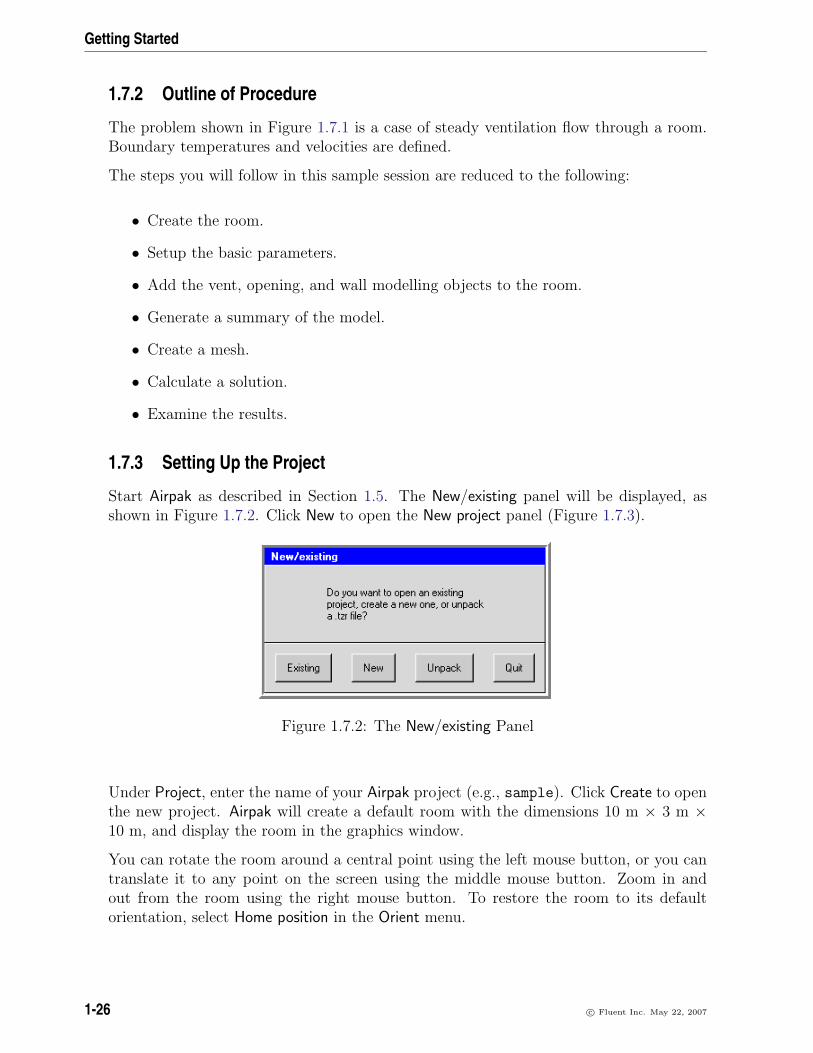
Getting Started
1.7.2 Outline of Procedure
The problem shown in Figure 1.7.1 is a case of steady ventilation flow through a room.Boundary temperatures and velocities are defined.
The steps you will follow in this sample session are reduced to the following:
• Create the room.
• Setup the basic parameters.
• Add the vent, opening, and wall modelling objects to the room.
• Generate a summary of the model.
• Create a mesh.
• Calculate a solution.
• Examine the results.
1.7.3 Setting Up the Project
Start Airpak as described in Section 1.5. The New/existing panel will be displayed, asshown in Figure 1.7.2. Click New to open the New project panel (Figure 1.7.3).
Figure 1.7.2: The New/existing Panel
Under Project, enter the name of your Airpak project (e.g., sample). Click Create to openthe new project. Airpak will create a default room with the dimensions 10 m × 3 m ×10 m, and display the room in the graphics window.
You can rotate the room around a central point using the left mouse button, or you cantranslate it to any point on the screen using the middle mouse button. Zoom in andout from the room using the right mouse button. To restore the room to its defaultorientation, select Home position in the Orient menu.
1-26 c© Fluent Inc. May 22, 2007

1.7 Sample Session
Figure 1.7.3: The New project Panel
1.7.4 Resizing the Room
To resize the room, ensure that the Room item in the Model node of the Model managerwindow is selected. Double click Room to display the Room edit panel.
In the Geometry tab, enter the coordinates shown in Table 1.7.1 into the Room editpanel. Click Update to resize the room. In the Orient menu, select Isometric view. Thiswill display an isometric view of the room scaled to fit the graphics window.
Table 1.7.1: Coordinates for the Room
xS 0.0 xE 4.57
yS 0.0 yE 2.74
zS 0.0 zE 2.74
1.7.5 Setting Up the Basic Parameters
You will begin by defining the species within the room and setting ambient temperatures.These parameters are specified in the Basic parameters panel. To open the Basic param-eters panel, select Basic parameters under the Problem setup node in the Model managerwindow.
Problem setup−→ Basic parameters
In the General setup tab of the Basic parameters panel, turn the IAQ/Comfort option Off,
c© Fluent Inc. May 22, 2007 1-27

Getting Started
Figure 1.7.4: The Room Panel (Geometry Tab)
because you will not be considering air quality issues. Turn On Species and click the Editbutton to open the Species definitions panel Figure 1.7.6).
Enter a value of 50 for the Initial concentration of h2o. Select RH from the menu next tothe Initial concentration entry field for h2o and click Accept to close the panel.
In the Default values tab of the Basic Parameters panel, enter new Ambient values for theproblem. Enter 20.56 for Temperature and 20.56 for Radiation temp. Click Accept tosave the new settings.
1-28 c© Fluent Inc. May 22, 2007

1.7 Sample Session
Figure 1.7.5: The Basic parameters Panel (General setup Tab)
c© Fluent Inc. May 22, 2007 1-29

Getting Started
Figure 1.7.6: The Species definitions Panel
1-30 c© Fluent Inc. May 22, 2007

1.7 Sample Session
1.7.6 Adding Objects to the Room
You will now add objects to the room. The process required to add an object involvesthree steps:
1. Create a new object.
2. Specify the location of the object.
3. Specify the flow and thermal characteristics of the object.
Adding a Rectangular Vent
First, you will create a vent to the back wall of the room. Click the button to create
a new vent, and then click the button to open the Vents panel (Figures 1.7.7 and1.7.8).
Figure 1.7.7: The Vents Panel (Geometry Tab)
c© Fluent Inc. May 22, 2007 1-31
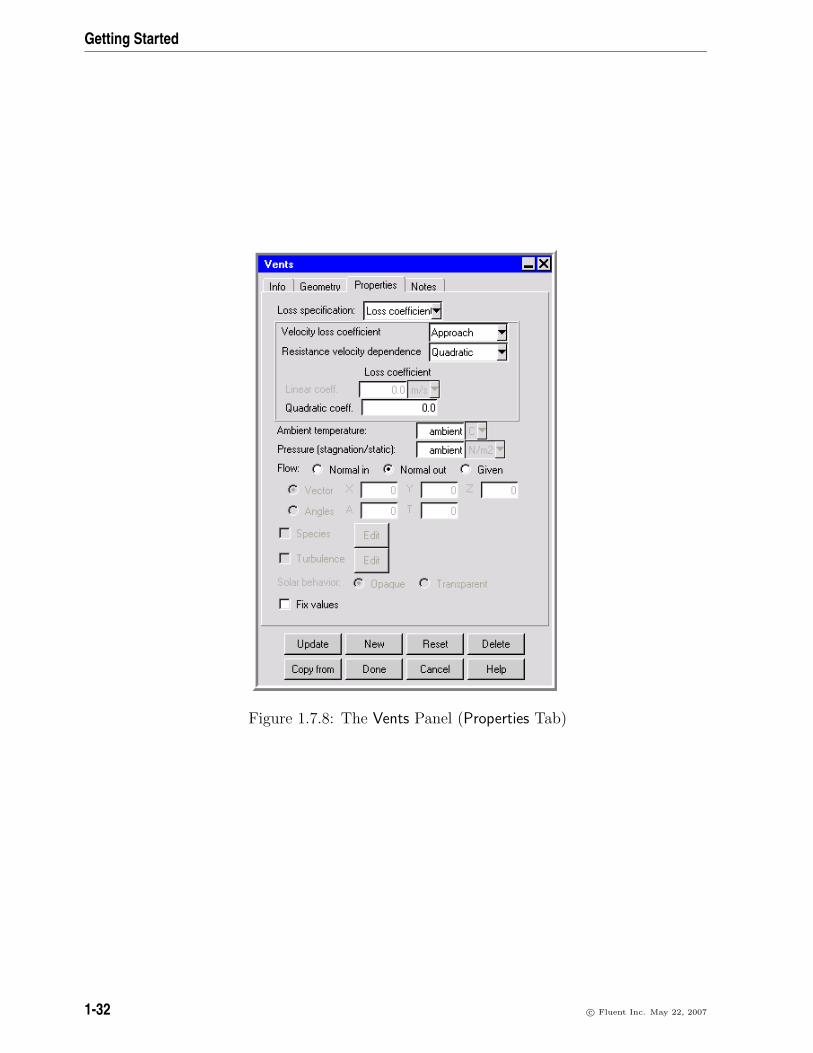
Getting Started
Figure 1.7.8: The Vents Panel (Properties Tab)
1-32 c© Fluent Inc. May 22, 2007

1.7 Sample Session
Click the Geometry tab. In the Plane drop-down list, select Y-Z to define the plane inwhich the vent lies. Under Specify by, enter the coordinates shown in Table 1.7.2 for thevent.
Table 1.7.2: Coordinates for the Vent
xS 0.0 xE —yS 0.0 yE 0.91
zS 2.29 zE 2.74
Click the Properties tab. Select Approach in the Velocity loss coefficient drop-down list.To specify that the vent is an outlet vent, keep the default option of Normal out for Flow.Click Done to accept all of the changes and close the panel.
i Note that you can also change the shape and size of the vent using the mouse. Holddown the <Shift> key on the keyboard and use the right mouse button to movethe vent’s boundaries. To translate the vent in the room, hold down the <Shift>
key and use the middle mouse button.
c© Fluent Inc. May 22, 2007 1-33

Getting Started
Adding an Opening
Next, you will add an opening on the front wall.
Click the button to create a new opening, and then click on the button toopen the Openings panel (Figures 1.7.9 and 1.7.10).
Figure 1.7.9: The Openings Panel (Geometry Tab)
1-34 c© Fluent Inc. May 22, 2007

1.7 Sample Session
Figure 1.7.10: The Openings Panel (Properties Tab)
c© Fluent Inc. May 22, 2007 1-35

Getting Started
Click the Geometry tab (Figure 1.7.9). In the Plane drop-down list, select Y-Z to definethe plane in which the opening lies. Enter the coordinates shown in Table 1.7.3.
Table 1.7.3: Coordinates for the Opening
xS 4.57 xE —yS 0.91 yE 1.83
zS 0.0 zE 0.46
Click the Properties tab (Figure 1.7.10). Select Temperature and enter a value of 20.56.Keep the default Velocity method of By component, select X Velocity and enter a value of-1.
Select Species and click Edit. This will open the Species concentrations panel (Fig-ure 1.7.11). Enter a value of 50 for the Concentration of h2o. Select RH from the menu tothe right of the Concentration entry field for h2o. Click Done in the Species concentrationspanel to accept the changes. Click Done in the Openings panel to accept all changes andclose the panel.
Figure 1.7.11: The Species concentrations Panel
Adding Walls
Finally, you will add walls to represent the boundaries of the room. For each pair ofparallel walls, you will create one wall and then copy it to create the opposing wall.
Adding the Floor and Ceiling
To construct the wall representing the floor, click the button to create a new wall,
and then click the button to open the Walls panel (Figures 1.7.12 and 1.7.13).
Click the Geometry tab. In the Plane drop-down list, select X-Z to define the plane inwhich the wall lies. Enter the coordinates shown in Table 1.7.4.
1-36 c© Fluent Inc. May 22, 2007

1.7 Sample Session
Figure 1.7.12: The Walls Panel (Geometry Tab)
Table 1.7.4: Coordinates for the Floor
xS 0.0 xE 4.57
yS 0.0 yE —–zS 0.0 zE 2.74
c© Fluent Inc. May 22, 2007 1-37

Getting Started
Figure 1.7.13: The Walls Panel (Properties Tab)
1-38 c© Fluent Inc. May 22, 2007

1.7 Sample Session
Click the Properties tab. Specify that the wall is at a constant temperature by selectingOutside temp under Thermal data and entering a value of 28.33.
Enable radiative heat transfer for the wall. Select Inner surface radiation and click Edit toopen the Radiation specification panel (Figure 1.7.14). Select All objects and click Accept.
In the Walls panel, click the Info tab and change the default wall name to floor in theName field. Click Done to accept all the changes and close the panel.
Figure 1.7.14: The Radiation specification Panel
Next, you will create the wall representing the ceiling by copying the first wall (floor)
to the appropriate location. Select the floor object and and click the button toopen the Copy wall floor panel (Figure 1.7.15). Alternatively, you can right-click the floorobject item to open the panel.
Select Translate and specify a Y offset of 2.74. Click Apply to complete the process anddisplay the copy (floor.1) in the Model manager window.
In the wall Edit panel for floor.1, change the default Name to ceiling. Click Apply toaccept the changes.
Adding the Back and Front Walls
To construct the back wall, click the button to create a new wall, and then click
the button to open the Walls panel.
In the Geometry tab, select Y-Z under Plane to define the plane in which the wall lies.Enter the coordinates shown in Table 1.7.5 for the wall.
Follow the procedure described above for the floor to specify an Outside temp of 28.33 andInner surface radiation on All objects. Click Done in the Walls panel to accept the changesand close the panel. In the wall Edit panel, change the default Name to wall-back.
c© Fluent Inc. May 22, 2007 1-39

Getting Started
Figure 1.7.15: The Copy wall floor Panel
Table 1.7.5: Coordinates for the Back Wall
xS 0.0 xE —yS 0.0 yE 2.74
zS 0.0 zE 2.74
1-40 c© Fluent Inc. May 22, 2007

1.7 Sample Session
Next, follow the procedure described above for copying the floor to create the ceiling tocopy the back wall to the front wall. Copy wall-back with an X offset of 4.57, a Y offsetof 0, and a Z offset of 0. Click Done to accept the changes and close the panel. In thewall Edit panel, change wall-back.1 to wall-front in the Name field. (Note that youwill not be able to see the entire name in the Name field.)
Adding the Right and Left Walls
To construct the right wall, click the button to create a new wall, and then click
the button to open the Walls panel.
In the Geometry tab, select X-Y and enter the coordinates shown in Table 1.7.3.
Table 1.7.6: Coordinates for the Right Wall
xS 0.0 xE 4.57
yS 0.0 yE 2.74
zS 0.0 zE —–
Follow the procedure described above for the floor to specify an Outside temp of 28.33 andInner surface radiation on All objects. Click Done in the Walls panel to accept the changesand close the panel. In the wall Edit panel, change the default Name to wall-right andclick Accept.
Next, follow the procedure described above for copying the floor to create the ceiling tocopy the right wall to the left wall. Copy wall-right with an X offset of 0, a Y offset of 0,and a Z offset of 2.74. Click Done to accept the changes and close the panel. In the wallEdit panel, change wall-right.1 to wall-left in the Name field and click Accept. Thefinished model should appear as shown in Figure 1.7.16.
c© Fluent Inc. May 22, 2007 1-41

Getting Started
Figure 1.7.16: Room with Intake Opening, Exhaust Vent, and Walls
1-42 c© Fluent Inc. May 22, 2007

1.7 Sample Session
1.7.7 Generating a Summary
Once you have completed your model, you can display a summary of the model byselecting Summary (HTML) in the View menu.
View−→Summary (HTML)
The HTML version of the summary will be displayed in your web browser. Airpak willautomatically launch your web browser (Netscape or IE), as shown in Figure 1.7.17.
Figure 1.7.17: Summary of the Model
c© Fluent Inc. May 22, 2007 1-43

Getting Started
1.7.8 Creating a Mesh
Once you are satisfied with your model, you can generate a mesh for it. First, you willcreate a default mesh, then you will display the mesh, and finally you will refine themesh.
1.7.9 Changing the Meshing Priority
You will need to change the order in which the objects in the room are meshed so thatroom objects in contact with the walls will receive a higher priority than the walls in themeshing process. Click Edit priorities in the Model menu to open the Object priority panel(Figure 1.7.18).
Model−→Edit priorities
Figure 1.7.18: The Object priority Panel
Enter a value of 0 for floor, ceiling, wall-back, wall-front, wall-right, and wall-left.
Click Accept to modify the priorities and close the panel.
Creating a Coarse Mesh
You will now generate a coarse mesh for your model. To create a mesh, select Generatemesh in the Model menu.
1-44 c© Fluent Inc. May 22, 2007

1.7 Sample Session
Model−→Generate mesh
Airpak will open the Mesh control panel, as shown in Figure 1.7.19. Alternatively, you
can click the button to open the Mesh control panel.
Figure 1.7.19: The Mesh control Panel
c© Fluent Inc. May 22, 2007 1-45

Getting Started
Turn off the Max X size, Max Y size, and Max Z size options. In the Mesh parametersdrop-down list under Global settings, select Coarse.
Click Generate mesh to generate a mesh using the coarse mesh parameters to representthe geometry.
The Message window will display the results of the mesh generation procedure, includ-ing the number of elements or “hexas” (hexahedral brick elements), and informationregarding the quality of the elements in the mesh. The number of mesh elements andthe number of nodes in the mesh will also be displayed in the Mesh control panel. TheMessage window will also report the volumetric flow rate required to change the air inthe room once per hour.
Displaying the Mesh
Airpak offers several options for displaying the mesh, including views on surfaces, withinthe entire room volume, and through a plane intersecting the room (a “plane-cut” view).
Viewing a Plane Cut Through the Mesh
To simplify the display of the mesh within the room, it is often useful to create a plane-cutview (i.e., a zero-thickness slice through the mesh).
Click the Display tab in the Mesh control panel and select the Cut plane option. Keepthe default settings of (0, 0, 1.37) for (PX, PY, PZ) and (0, 0, 1) for (NX, NY, NZ) forthe Plane location. These settings will result in a mesh display on an x-y plane passingthrough the point (0, 0, 1.37).
Display the mesh on the plane cut by selecting Display mesh. Move the slider bar be-low the Plane location coordinates to adjust the plane cut so that it is at the opening(Figure 1.7.20).
In general, when you view a mesh, there are a few things to look for:
In general:
• A “good” mesh should include a minimum of three nodes (four elements) in thechannels between objects that are close to one another.
• The aspect ratio of the largest to smallest elements should not be less than 1 to 10(0.1).
• Elements should be graded away from object surfaces (i.e., there should be no largejumps in size for elements near surfaces in the model).
1-46 c© Fluent Inc. May 22, 2007

1.7 Sample Session
Figure 1.7.20: A Plane-Cut View of the Mesh
Refining the Mesh
For this example, the coarse mesh shown in Figure 1.7.20 is not sufficient to generatean accurate solution. Airpak provides tools to improve the mesh. You will change theglobal specification of the maximum element size to refine the mesh and improve themesh quality.
To specify the maximum element size throughout the computational domain, click on theGenerate tab in the Mesh control panel. Select the Max X size, Max Y size, and Max Z sizeoptions in the Mesh control panel, and enter values of 0.25, 0.25, and 0.25, respectively.Under Global settings, select Normal in the Mesh parameters drop-down list.
Click Generate mesh to generate the refined mesh. The refined mesh (Figure 1.7.21) willbe displayed in the graphics window automatically because Display mesh is still selectedin the Display section of the Mesh control panel. You can use the two square boxes toadvance the plane cut and view the mesh throughout the model.
To turn off the mesh display, click the Display tab at the top of the Mesh control paneland deselect the Display mesh option. Then Close the Mesh control panel.
1.7.10 Checking the Flow Regime
Before starting the solver, you will first review estimates of the Reynolds and Pecletnumbers to check that the proper flow regime is being modeled.
Check the values of the Reynolds and Peclet numbers by opening the Solver setup panel(Figure 1.7.22).
c© Fluent Inc. May 22, 2007 1-47

Getting Started
Figure 1.7.21: Plane-Cut View of the Refined Mesh
1-48 c© Fluent Inc. May 22, 2007

1.7 Sample Session
Solve−→Settings−→Basic
Figure 1.7.22: The Basic settings panel
Click the Reset button. Check the values printed to the Message window. The Reynoldsand Peclet numbers are approximately 31,000 and 23,000, respectively, so the flow isturbulent. Since you are currently modeling turbulent flow, no changes are required. TheMessage window will also report that the initial air velocity has been reset to −10−4 timesgravity. This modification improves the convergence of natural convection calculations.
Click Accept to save the new solver settings.
1.7.11 Saving the Model
You should save your model (including the mesh) before you calculate a solution for yourmodel. You must save the project for your current session in order to continue youranalysis in a future Airpak session. To save the project, select Save project in the Filemenu.
File−→Save project
1.7.12 Calculating a Solution
After the mesh has been generated and refined, Airpak is ready to solve the model.
c© Fluent Inc. May 22, 2007 1-49

Getting Started
Set the Solution Parameters
To review the default solution parameters, double click the Basic settings item under theSolution settings node of the Model manager window.
Solution settings−→ Basic settings
Airpak will open the Basic settings panel, as shown in Figure 1.7.22.
Figure 1.7.23: The Basic settings Panel
Increase the Number of iterations to 300 and keep the default values for the remainingsettings (Figure 1.7.23). Click Accept to accept the solution parameters.
Calculating
You will use the Solve panel (Figure 1.7.24) to start the solver. To open the Solve panel,select Run solution in the Solve menu.
Solve−→Run solution
1-50 c© Fluent Inc. May 22, 2007

1.7 Sample Session
Figure 1.7.24: The Solve Panel (Options tab)
The default Solution ID consists of the project name and a sequential two-digit suffix(starting value = 00). To modify the Solution ID, you can type a new name in theSolution ID text entry box. In this example, you will keep the default ID.
Click Start solution to start the solver. The solver will start the calculation, and Airpakwill open the Solution residuals graphics display and control window, where it will displaythe convergence history for the calculation.
The solution is converged to the default tolerances after a total of about 100 iterations.At this point, your residual plot will look something like Figure 1.7.25. Note that theexact number of iterations required for convergence may vary on different computers.Also the actual values of the residuals may differ slightly on different machines, so yourplot may not look exactly the same as Figure 1.7.25.
Click Done to close the Solution residuals window.
c© Fluent Inc. May 22, 2007 1-51

Getting Started
Figure 1.7.25: Residuals After Convergence
1-52 c© Fluent Inc. May 22, 2007

1.7 Sample Session
1.7.13 Examining the Results
Airpak provides a number of ways to view and examine the solution results, including:
• object-face views
• plane-cut views
• isosurface views
• point views
• variation plots
The following sections illustrate how to generate and display each view.
Object-Face Views
An object-face view allows you to examine the distribution of a solution variable on oneor more faces of an object in the model. To generate an object-face view, you mustselect the object and specify both the variable to be displayed (e.g., temperature) andthe attributes of the view (e.g., shading type).
You will use the Object face panel (Figure 1.7.26) to create a solid-band object-face viewof the temperature distribution on the vent. To open the Object face panel, select Objectface in the Post menu.
Post−→Object face
To specify the vent as the object on which the results will be displayed, select vent.1 inthe Object drop-down list, and click Accept.
To specify the variable to be displayed and the attributes of the view, turn on the ShowContours option and click Parameters. This will open the Object face contours panel,shown in Figure 1.7.27.
c© Fluent Inc. May 22, 2007 1-53

Getting Started
Figure 1.7.26: The Object face Panel
Figure 1.7.27: The Object face contours Panel
1-54 c© Fluent Inc. May 22, 2007

1.7 Sample Session
The default Variable is Temperature, so no change is needed. Keep the default selectionsof Solid under Contour options and Banded under Shading options. Keep the default optionof Fixed for Level spacing. Under Color levels, choose Visible on screen from the Calculateddrop-down list and click Done to accept the settings and close the Object face contourspanel.
Click Create in the Object face panel to create and display the object face by loading thedata. The solid-band temperature contours on the vent will be displayed in the graphicswindow. Select Orient negative X in the Orient menu and then use the Zoom in featureon the menu to get a close-up view of the contours on the vent (Figure 1.7.28).
In addition to the solid contour bands on the vent, Airpak displays a legend showing avertical color-band spectrum and the associated temperatures in the graphics window.The spectrum includes the entire range of temperatures applicable to the solution.
Figure 1.7.28: Contours of Temperature on the Vent
i Before continuing, you should deactivate the line band contour plot so that itwill not obstruct your view of subsequent postprocessing objects. In the Objectface panel, deselect Active and click Done. If the Object face panel is not visibleon your screen, double click the face.1 item under the Postprocessing node of the
c© Fluent Inc. May 22, 2007 1-55

Getting Started
Model manager window to bring the Object face panel to the foreground. Oncedeactivated, the face.1 item will appear in the Inactive node of the Model managerwindow.
Plane-Cut Views
Plane-cut views allow you to observe the variation in a solution variable across the surfaceof a plane.
Select Home position in the Orient menu to return the room to its default orientation(front view).
You will use the Plane cut panel (Figure 1.7.29) to view the direction and magnitude ofvelocity across a horizontal plane near the middle of the room. To open the Plane cutpanel, select Plane cut in the Post menu.
Post−→Plane cut
Figure 1.7.29: The Plane cut Panel
To specify a horizontal plane cut, select Horizontal - screen select in the Set position drop-down list under Plane location. To create a cut plane, click a point in the graphics windowabout 1/3 from the top of the vent using the left mouse button. Turn on the Show vectorsoption and click Done. Select Orient positive Y in the Orient menu to see a top-down viewof the room. Then click on Scale to fit in the Orient menu to see the view of the room,as shown in Figure 1.7.30.
1-56 c© Fluent Inc. May 22, 2007

1.7 Sample Session
Note that depending on where you click in the graphics display, you will see differentvelocity vectors. If you wish to see Figure 1.7.30 exactly, refer to Figure 1.7.29 and enterthe displayed coordinates for (PX, PY, PZ) and (NX, NY, NZ).
Figure 1.7.30: Velocity Vectors (Plane-Cut View)
i To deactivate the plane-cut view, right click the cut.1 item under the Postprocessingnode of the Model manager window, deselect Active in the pull-down menu. Oncedeactivated, the cut.1 item will appear in the Inactive node of the Model managerwindow.
c© Fluent Inc. May 22, 2007 1-57

Getting Started
Isosurface Views
Isosurface views display surfaces across which one of the primary or derived variablesexhibits a single value. First, select Isometric view from the Orient menu to display theisometric view of the room.
Next, you will use the Isosurface panel (Figure 1.7.31) to view the surface across whichall points have a temperature of 25C. To open the Isosurface panel, select Isosurface inthe Post menu.
Post−→Isosurface
Figure 1.7.31: The Isosurface Panel
In the Isosurface panel, keep the default Variable of Temperature. Enter a value of 25
next to Value to specify an isosurface at 25C. Select the Show contours and Show vectorsoptions. Click Done to create the isosurface, an isometric view of which is shown inFigure 1.7.32.
1-58 c© Fluent Inc. May 22, 2007

1.7 Sample Session
Figure 1.7.32: Isosurface of Temperature = 25 Degrees
i To deactivate the isosurface view, right click the iso.1 item under the Postprocessingnode in the Model manager window and deselect the Active option in the pull-downmenu. Once deactivated, the ice.1 item will appear in the Inactive node of the Modelmanager window.
Point Views
Point views allow you to probe the computational domain to sample the values of one ofthe primary or derived solution variables at any point.
You will use the Point panel (Figure 1.7.33) to probe for temperature. To open the Pointpanel, select Point in the Post menu.
Post−→Point
Keep the default Variable of Temperature. In the Position drop-down list, enter 1 1 1 tocreate a starting point offset from the origin. Select Leave trail to enable tracing. Keepthe default Point size of 4. Click Done to create the point and close the panel.
Airpak draws the initial (blue) sample point at the x, y, and z coordinates specified (11 1) and displays the temperature at that point on the postprocessing Edit window nextto Value, as shown in Figure 1.7.34.
c© Fluent Inc. May 22, 2007 1-59

Getting Started
Figure 1.7.33: The Point Panel
Figure 1.7.34: The Postprocessing Edit Window for a Point View
1-60 c© Fluent Inc. May 22, 2007

1.7 Sample Session
You can sample the temperature at a different location in the domain by moving thepoint. Select the point in the graphics window by holding down the <Shift> key on thekeyboard and using the left mouse button to select the point. Drag the point to the newlocation using the left mouse button. As the point moves, it will leave behind a tracecolored according to the temperature legend in the graphics window. The postprocessingEdit window displays the value of the temperature at the current location (Value), andthe minimum (Global min) and maximum (Global max) values of temperature in thecomputational domain.
i To deactivate the point trace before moving on, right click the point.1 item underthe Postprocessing node in the Model manager window, and deselect the Activeoption in the pull-down menu. Once deactivated, the point.1 item will appear inthe Inactive node of the Model manager window.
Variation Plots
Airpak variation plots allow you to view the variation of any one of the primary or derivedsolution variables along a line through the computational domain.
First, select Home position in the Orient menu to return the room to its default orientation(front view).
You will use the Variation plot panel (Figure 1.7.35) to view temperature along a horizontalline in the middle of the room. To open the Variation plot panel, select Variation plot inthe Post menu.
Post−→Variation plot
Keep the default Variable of Temperature. Specify a variation plot line normal to thescreen at a point by clicking the From point objects button and entering the values 0.1,1.0, 2.5 under Point and 0, 0, 1 under Direction. Click Create in the Variation plotpanel to create a variation plot, as shown in Figure 1.7.36. Click Dismiss to close thepanel.
Airpak draws the variation plot in a separate window (called the Variation of Temperaturegraphics display and control window in this example), and displays the line on which thevariation plot is calculated in the graphics window. You can use the mouse to rotatethe room and view the variation plot line from various angles. Click Done to close theVariation of Temperature window and remove the variation plot line from the graphicswindow. Note that you can also create a plot by clicking the From screen button in theVariation plot panel and then clicking a point in the graphics window.
c© Fluent Inc. May 22, 2007 1-61

Getting Started
Figure 1.7.35: The Variation plot Panel
Saving Postprocessing Objects
You can save the objects (e.g., plane-cut views, isosurfaces) generated during the post-processing session to a file, so that you can reuse them the next time you view the modelin Airpak. Select Save post objects to file in the Post menu.
Post−→Save post objects to file
Click Save in the resulting File selection dialog box to save the file with the default namepost objects.
i Saving postprocessing objects often requires a large amount of disk space.
1.7.14 Generating Reports
Airpak allows you to generate, view, and print reports detailing the results of the simu-lation. Reports regarding primary and derived solution variables such as temperature,flow rate, heat flux, and heat transfer coefficient can be generated either for individualobjects or for collections of objects.
You will use the Full report panel (Figure 1.7.37) to generate an on-screen report of massflow rate for the fan. To open the Full report panel, select Full report in the Report menu.
1-62 c© Fluent Inc. May 22, 2007

1.7 Sample Session
Figure 1.7.36: Variation of Temperature Plot
c© Fluent Inc. May 22, 2007 1-63

Getting Started
Report−→Full report
Figure 1.7.37: The Full report Panel
To specify mass flow rate as the variable to be reported, select Mass flow in the Variabledrop-down list. Select the Specific objects option under Report region and select vent.1 inthe adjacent drop-down list, and click Accept to specify the fan as the object on whichthe results will be reported. Select the Sides option to create a report for the wholefan. Keep the Write to window option turned on to display the report in a window, anddeselect the Write to file option. Click Write to generate the report. Airpak displays thereport in a separate window (called the Full report for Mass flow window in this example),as shown in Figure 1.7.38. Airpak displays the surface area of the fan, and the average,maximum, and minimum values for the mass flow rate. Click Done to close the Reporton Mass flow window.
1-64 c© Fluent Inc. May 22, 2007

1.7 Sample Session
Figure 1.7.38: The Full report for Mass flow Window
1.7.15 Exiting From Airpak
When you are finished examining the results, you can end the Airpak session by clickingQuit in the File menu.
File−→Quit
c© Fluent Inc. May 22, 2007 1-65

Getting Started
1.7.16 Summary
This example has been designed to show you how to use Airpak to solve a very simpleproblem. Example problems of increasing difficulty are solved in the Airpak TutorialGuide, where the different modeling objects, physical models, and solution parametersthat are available in Airpak are illustrated in greater detail.
1-66 c© Fluent Inc. May 22, 2007

Chapter 2. User Interface
The user interface for Airpak consists of a graphical interface with windows, menus,toolbars, and panels. An overview of the graphical interface, including information aboutthe toolbars, menus, and panels is presented in this chapter. Details on using the mouseand keyboard and accessing the on-line help are also included.
• Section 2.1: The Graphical User Interface
• Section 2.2: Using the Mouse
• Section 2.3: Using the Keyboard
• Section 2.4: Quitting Airpak
2.1 The Graphical User Interface
Airpak’s graphical user interface (GUI) consists of several major components: the menubar, toolbars, control panels, the Model manager window, the Message window, and thegraphics windows. When you use the GUI, you will be interacting with one of thesecomponents at all times within a single Airpak application window.
You interact with Airpak through the GUI by means of the mouse and the keyboard. Toperform most operations in Airpak, you simply position the cursor of the mouse on theobject or item you wish to act upon, and click the left mouse button.
You perform most tasks (e.g., file saving, object creation, object editing, etc.) usingeither the menu bar, the toolbars, or the Model manager window. Your work is displayedin the graphics window, where you can use the mouse to view various aspects of yourmodel.
Information about the components of the GUI is presented in the following sections:
• Section 2.1.1: The Main Window
• Section 2.1.2: The Airpak Menus
• Section 2.1.3: The Airpak Toolbars
• Section 2.1.4: The Model manager Window
• Section 2.1.5: The Graphics Windows
c© Fluent Inc. May 22, 2007 2-1

User Interface
• Section 2.1.6: The Message Window
• Section 2.1.7: The Edit Window
• Section 2.1.8: File Selection Dialog Boxes
• Section 2.1.9: Control Panels
• Section 2.1.10: Accessing On-line Help
2.1.1 The Main Window
When you start Airpak, the Main window (center) is displayed on the screen (Figure 2.1.1).The Main window controls the execution of the Airpak program and has six primarycomponents: the Main Menu bar (top), the Model Display window or graphics window(right), the Model manager window (left), the Message window (lower left), the Editwindow (lower right), and several toolbars.
Resizing Airpak Windows
You can customize the appearance of the Main window by resizing any of the four majorAirpak windows: the Model manager window; the Message window; the Edit window; andthe Model Display graphics window.
To resize an Airpak window, click and hold down the left mouse button on the separatorand drag the separator to the desired location. The slider bars for each Airpak windoware located either to the lower right and/or the lower left of each window.
2.1.2 The Airpak Menus
The Main Menu bar (Figure 2.1.2) contains twelve menus that are located along the topof the Main window. These menus (File, Edit, View, Orient, Model, Tree, Macros, Solve,Post, Report, Windows, and Help) are accessible at all times and allow you to access top-level Airpak functionality. When you select one of these menus in the Main Menu bar, aset of menu-specific options will be displayed. Some menu-specific options also have sub-options that you can choose from. In addition, note that each menu in the Main Menubar has a keyboard shortcut so that the menu and its options can be accessed using thekeyboard. For more information on using the keyboard in Airpak, see Section 2.3.
The File Menu
The File menu (Figure 2.1.3) contains options for working with Airpak projects and projectfiles. From this menu, you can open, merge, and save Airpak projects. In addition, youcan import, export, compress, and decompress files relating to your Airpak model. Thereare also utilities designed to save or print your model geometries. A brief description
2-2 c© Fluent Inc. May 22, 2007
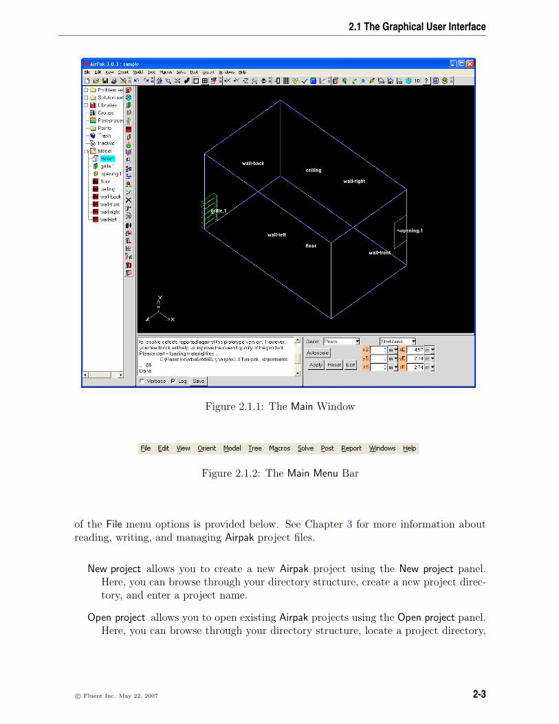
2.1 The Graphical User Interface
Figure 2.1.1: The Main Window
Figure 2.1.2: The Main Menu Bar
of the File menu options is provided below. See Chapter 3 for more information aboutreading, writing, and managing Airpak project files.
New project allows you to create a new Airpak project using the New project panel.Here, you can browse through your directory structure, create a new project direc-tory, and enter a project name.
Open project allows you to open existing Airpak projects using the Open project panel.Here, you can browse through your directory structure, locate a project directory,
c© Fluent Inc. May 22, 2007 2-3

User Interface
Figure 2.1.3: The File Menu
and either enter a project name, or specify an old project name from a list of recentprojects. Additionally, you can specify a version name or number for the project.
Merge project allows you to merge an existing project into your current project usingthe Merge project panel.
Reload main version allows you to re-open the original version of the Airpak projectwhen your project has multiple versions. See Chapter 6 for more information.
Save project saves the current Airpak project.
Save project as allows you to save the current Airpak project under a different nameusing the Save project panel.
Import provides options to import IGES, DXF, and tetin file geometries into Airpak.You also can import DWG and IFC files, as well as comma separated values orspreadsheet format (CSV) using this option. See Chapter 4 for more informationabout importing files.
Export allows you to export your work to IGES files as well as comma separated valuesor spreadsheet format (CSV/Excel) files. See Chapter 4 for more information aboutexporting files.
Unpack project opens a File selection dialog that allows you to browse for and decom-press .tzr files.
2-4 c© Fluent Inc. May 22, 2007

2.1 The Graphical User Interface
Pack project opens a File selection dialog that allows you to compact your project intoa compressed .tzr file.
Email project allows you to pack and email your project by specifying the Recipientemail address, Subject for email, and Message text. See Section 27.13 for moreinformation on emailing the project.
Cleanup allows you to clean up your project by removing or compressing data relatingto mesh, post-processing, screen captures, summary output, reports, and scratchfiles using the Clean up project data panel.
Print screen allows you to print a PostScript image of the Airpak model that is dis-played in the graphics window using the Print options panel. The inputs for the Printoptions panel are similar to those in the Graphics file options panel. See Section 3.5for details.
Create image file opens a Save image dialog that allows you to save your model dis-played in the graphics window to an image file. Supported file types include: GIF,JPEG, PPM, TIFF, VRML, and PS.
Shell window opens a separate window running an operating system shell. The windowis initially in the subdirectory of the Airpak projects directory that contains all thefiles for the current projects. In this window you can issue commands to theoperating system without exiting Airpak. Type exit in the window to close thewindow when you are finished using it. Note that on Windows machines, this menuitem appears as Command prompt.
Quit exits the Airpak application. See Section 2.4 for details.
The Edit Menu
The Edit menu (Figure 2.1.4) contains options for editing your Airpak model. A descrip-tion of the Edit menu options is provided below. See Chapter 7 for more informationabout editing objects in your Airpak model.
Figure 2.1.4: The Edit Menu
c© Fluent Inc. May 22, 2007 2-5

User Interface
Undo allows you to undo the last model operation you performed. Undo can be usedrepeatedly to take you back to the first operation performed.
Redo allows you to redo one or more previously undone operations. This option appliesonly to operations undone by selecting the Undo option.
Preferences opens the Preferences panel, where you can configure the graphical userinterface. See Section 6.3 for more information about setting preferences.
Annotations allows you to add annotations (e.g., labels and arrows) to the graphicswindow using the Annotations panel. See Section 2.1.5 for more information aboutannotations.
Current object allows you to perform various operations on the currently selected ob-ject in the model. Options include:
Modify applies any changes you have made to the object.
Reset resets settings for the current object to the values it had when the projectwas opened or to when the object settings were last updated.
Copy from opens the Object selection panel, where you can select and copy otherobjects in your model.
Move opens an object-specific Move panel, where you can scale, rotate, translate,or mirror an object.
Copy opens an object-specific Copy panel, where you can create a copy of anobject and then scale, rotate, translate, or mirror the copied object.
Edit opens an object-specific Edit window, where you can set various objectproperties.
Delete removes the object from the model.
Active allows you to toggle the object’s activity.
Remove from group allows you to remove the object from its group.
Current group allows you to perform various operations on the selected group of objectsin the model. Options include:
Create creates a new group.
Add to group allows you to add objects to a group either by selecting a point orregion on the screen or choosing an object name or pattern.
Remove from group allows you to remove objects from a group either by selectinga point or region on the screen or choosing an object name or pattern.
Rename allows you to rename a group.
Delete removes the selected group from the model.
2-6 c© Fluent Inc. May 22, 2007

2.1 The Graphical User Interface
Copy opens a group-specific Copy panel, where you can create a copy of a groupand then scale, rotate, translate, or mirror the copied group.
Move opens a group-specific Move panel, where you can scale, rotate, translate,or mirror a group.
Edit opens a group-specific Edit window, where you can set various group prop-erties.
Activate all activates all objects in the selected group.
Deactivate all deactivates all objects in the selected group.
Delete all removes all objects from the selected group and the Airpak model.
Create assembly creates an assembly from the selected group and adds the as-sembly to the Airpak model.
Copy params applies the parameters of the selected object to all objects of thesame type in the selected group.
Save as project allows you to save the group as an Airpak project.
The View Menu
The View menu (Figure 2.1.5) contains options that control the appearance of the graphicswindow. A description of the View menu options is provided below.
Figure 2.1.5: The View Menu
c© Fluent Inc. May 22, 2007 2-7

User Interface
Summary (HTML) allows you to display an HTML version of the summary of yourmodel. To display the summary, select Summary (HTML) in the View menu. Air-pak will automatically launch your web browser (e.g., Netscape, IE), as shown inFigure 1.7.17.
Location allows you to display the coordinates of a point in your model. To find thecoordinates of a point, select Location in the View menu. Select the point in thegraphics window using the left mouse button. Airpak will display the coordinatesof the point you select in the graphics window and in the Message window. To exitfrom the Location mode, click with the right mouse button in the graphics window.
Distance allows you to calculate the distance between two points in your Airpak model.To find the distance between two points, select Distance in the View menu. Selectthe first point in the graphics window using the left mouse button. Airpak willdisplay the coordinates of the point you select in the graphics window and in theMessage window. Then select the second point in the graphics window, also usingthe left mouse button. Airpak will display the coordinates of the second point inthe graphics window and in the Message window, calculate the distance betweenthe two points, and display the distance in the Message window. To exit from theDistance mode, click with the right mouse button in the graphics window.
Angle allows you to calculate the angle created between two vectors in your Airpakmodel. To find the angle between two vectors, select Angle in the View menu. Selecta vertex point in the graphics window using the left mouse button. Then select theend point of the first vector, also using the left mouse button. Then select the endpoint of the second vector, also using the left mouse button. Airpak will display theangle created by the two vectors in the Message window.
Bounding box allows you to determine the minimum and maximum coordinates foryour model’s bounding box. To find the minimum and maximum coordinates forthe model’s bounding box, select Bounding box in the View menu. Airpak will displaythe minimum and maximum x, y, and z coordinates for the model enclosure in theMessage window.
Markers allows you to add or remove markers from the graphics window of your Airpakmodel.
Add allows you to add a marker to the graphics window of your Airpak model.To add a marker, select Markers then select Add in the View menu. This willopen the Add marker panel (Figure 2.1.6).
To specify the position of the marker, you can enter the coordinates of thepoint (separated by spaces) next to Position or you can click on the Selectbutton and then click on a location in the graphics window to select the point.To specify the text for the marker, enter the text in the Text box. Click Acceptto add the marker to the graphics window.
2-8 c© Fluent Inc. May 22, 2007

2.1 The Graphical User Interface
Figure 2.1.6: The Add marker Panel
Clear allows you to remove all of the markers from the graphics window.
Rubber bands allows you to add and remove rubber-banding rulers between two objectsin the graphics window.
Add allows you to add a rubber-banding ruler between two points on two objectsin the graphics window. To add a rubber band, select Add in the View menu.Select the point on the first object in the graphics window using the leftmouse button. Then select the point on the second object in the graphicswindow, also using the left mouse button. Airpak will calculate the overalldistance between the two points, and the distances in the x, y, and z coordinatedirections. It will display this information in the graphics window next to anarrow drawn between the objects. If you move one of the objects, Airpak willupdate the display of the distances between the two objects.
Clear removes all of the rubber bands from the graphics window.
Set background allows you to set the background color of the graphics window. Toset the background color, select Set background from the View menu and use themethod or panel that is appropriate to your system.
Edit toolbars allows you to customize the appearance of Airpak by displaying or hidingany of the Airpak toolbars using the Available toolbars panel (Figure 2.1.7).
By default, all toolbars are visible. To hide toolbars, deselect the appropriate tool-bar option and click Accept. Click Reset to display all previously hidden toolbars.
Shading contains options that control the rendering of your Airpak model. Optionsinclude:
Wireframe outlines the model’s outer edges and those of its components. Neitherthe Solid nor the Selected solid option can be used with the Wireframe option.
Solid adds solid-tone shading to the visible surfaces of the model’s internal com-ponents to give them a solid appearance. Neither the Wireframe nor the Se-lected solid option can be used when Solid is selected.
Selected solid adds solid-tone shading to the visible surfaces of the object cur-rently selected in the object Edit window to give it a solid appearance. Neitherthe Wireframe nor the Solid option can be used when Selected solid is selected.
c© Fluent Inc. May 22, 2007 2-9

User Interface
Figure 2.1.7: The Available toolbars Panel
Hidden line activates the hidden line removal algorithm, which makes objectsthat are drawn to look transparent now appear to be solid.
Display contains options that allows you to customize the appearance of the graphicswindow. Options include:
Object names displays object names next to objects in the graphics window.Options include:
Current assembly displays the names of the objects in the currently selectedassembly.
None does not display any object names. This option is selected by default.
Selected displays the names of the currently selected objects.
Coord axes displays the coordinate axes reference in the lower left hand cornerof the graphics window. This option is selected by default.
Visible grid displays the grid in the graphics window. The grid parameters mustfirst be set in the Interaction section of the Preferences panel. See Section 6.3.7for more information about the interactive editing.
Origin marker displays the origin of the graphics window. This option is selectedby default. You can move the origin marker after it is displayed by holdingdown the <Control> key, clicking on the origin marker with the middle mousebutton, and dragging it to a new location.
Rulers displays ruled coordinate axes from the origin of the graphics window.
Project title displays the project name and the Airpak version number in thegraphics window. You can move the project title after it is displayed by
2-10 c© Fluent Inc. May 22, 2007
2.1 The Graphical User Interface
holding down the <Control> key, clicking on the project title with the middlemouse button, and dragging it to a new location.
Current date displays the current date in the graphics window. You can movethe current date after it is displayed by holding down the <Control> key,clicking on the current date with the middle mouse button, and dragging itto a new location.
Construction lines displays construction lines from IGES models.
Construction points displays construction points from IGES models.
Mesh displays a mesh that has been loaded into a model.
Mouse position displays the position of the mouse in the lower left hand portionof the graphics window.
Depthcue adds a visual element of depth to enhance the model’s 3D appear-ance. This effect is achieved by intensifying foreground lines and softeningbackground lines. This option does not affect the X Window graphics driver.
Visible allows you to choose which objects of your Airpak model that you want dis-played in the graphics window. You can toggle the visibility of the following items:
Room
Blocks
Fans
Vents
Openings
Persons
Walls
Partitions
Sources
Resistances
Heat exchangers
Hoods
Assemblies
Wires
To make any of these items become visible (or invisible) in the display, select (ordeselect) the desired sub-option. Hidden objects appear in the Model managerwindow as grayed-out items under the Inactive node but are not visible in thegraphics window. This allows you to view and edit portions of your model whilehiding the rest from view.
c© Fluent Inc. May 22, 2007 2-11

User Interface
Action turns on objects that have motion associated with them, such as fans. Thisanimation option uses considerable CPU time, and it is recommended that thisoption should not be left on, but used only as needed. The motion has no physicalsignificance, and is intended only to aid in the recognition of model components.
Lights allows you to set the lighting parameters for viewing your Airpak model. Tochange the lighting parameters, select Lights in the View menu. This will open theLighting options panel (Figure 2.1.8).
Figure 2.1.8: The Lighting options Panel
Under Advanced lighting, you can choose Simple lighting (the default) or Complexlighting. In both cases, the lighting direction is fixed relative to your view of themodel. If Complex lighting is selected, you will have control over the Intensity andColor of the Ambient light, and the Intensity, Color, and direction of origin (X, Y,Z) of up to four additional lights. The Intensity may range from 0 to 1, and theColor can be specified as described in Section 6.3.6. You can enable or disable aparticular light by toggling the check box next to its name.
For Complex lighting, you can also specify how the object surface materials will
2-12 c© Fluent Inc. May 22, 2007

2.1 The Graphical User Interface
respond to being lit. Under Materials, you can use the slider bars or directly specifyvalues for the following parameters:
Diffuse reflectance is the ratio of the incident luminous flux reradiated in thevisual spectrum by diffuse reflection. Diffuse reflectance plays the most im-portant role in determining what you perceive the color of an object to be. Itis affected by the color of the incident diffuse light and the angle of the inci-dent light relative to the normal direction, with the highest intensity wherethe incident light falls perpendicular to the surface. The diffuse reflectance isnot affected by the position of your viewpoint. Values may range from 0 to 1.
Ambient reflectance is the ratio of the incident luminous flux reradiated in thevisual spectrum by ambient reflection. Ambient reflectance is most noticeablewhere an object receives no direct illumination. An object’s total ambientreflectance is affected by the global ambient light and ambient light fromindividual light sources. Like diffuse reflectance, ambient reflectance is notaffected by the position of your viewpoint. Values may range from 0 to 1.
Shininess controls the size and brightness of the highlight. Values may rangefrom 0 to 128. The higher the value, the smaller and brighter (more focused)the highlight.
Specular reflectance is the ratio of the incident luminous flux reradiated in thevisual spectrum by specular reflection. Specular reflection from an objectproduces highlights. Unlike diffuse and ambient reflection, the amount ofspecular reflection that you see does depend on the location of your viewpoint,and it is brightest along the direct angle of reflection. Values may range from0 to 1.
To restore the default values for complex lighting, click Restore complex defaults.
The Orient Menu
The Orient menu (Figure 2.1.9) contains options that allow you to modify the directionfrom which you view your model in the graphics window. Besides selecting the view alongthe x, y, or z axis, you can zoom your model, scale it to fit exactly within the graphicswindow, or restore it to the default view along the negative z axis. A description of theOrient menu options is provided below.
c© Fluent Inc. May 22, 2007 2-13

User Interface
Figure 2.1.9: The Orient menu
Home position selects the default view of your model directed along the negative zaxis.
Zoom in allows you to focus on any part of your model by opening and resizing awindow around the desired area. After selecting this option, position the mousepointer at a corner of the area to be zoomed, hold down the left mouse button anddrag open a selection box to the desired size, and then release the mouse button.The selected area will then fill the graphics window.
Scale to fit adjusts the overall size of your model to take maximum advantage of thegraphics window’s width and height.
Orient positive X, Y, Z views the model toward the direction of the positive x, y, or zaxis.
Orient negative X, Y, Z views the model toward the direction of the negative x, y, orz axis.
Isometric view views the model from the direction of the vector equidistant to all threeaxes.
Reverse orientation views the model along the current view vector but from the oppo-site direction (i.e., rotated 180 degrees).
Nearest axis orients the view to the nearest axis normal to the plane.
Save user view opens the Query panel (Figure 2.1.10) that prompts you for a viewname and then saves the current view using your specified name. The new viewname is attached to a listing of user views at the bottom of the Orient menu.
Clear user views removes the listing of user views from the bottom of the Orient menu.
2-14 c© Fluent Inc. May 22, 2007

2.1 The Graphical User Interface
Figure 2.1.10: The Query panel
The Model Menu
The Model menu (Figure 2.1.11) contains options that allow you to generate a mesh,load non-native files, edit CAD data, and perform other model-related functions. Adescription of the Model menu options is provided below.
Figure 2.1.11: The Model Menu
Generate mesh opens the Mesh control panel, where you can provide settings to createa mesh for your Airpak model. See Chapter 26 for more information about meshes.
CAD data opens the CAD data panel that allows you to import into Airpak and editgeometry that was created using a commercial CAD program. See Chapter 4 formore information about importing files into Airpak.
Radiation opens the Form factors panel, where you can model the radiation for specificobjects in your Airpak model. See Chapter 22 for more information about radiationmodels in Airpak.
Check model performs a check to test the model for problems in the design. SeeSection 7.9.2 for details.
Snap to grid opens the Snap to grid panel that allows you to snap a selected object inthe graphics window to the grid. See Section 7.3.7 for details.
Edit priorities opens the Object priorities panel that allows you to prioritize the objectsin your model. Airpak provides priorities based on object creation and uses thepriorities when meshing the model. See Section 26.7 for details.
c© Fluent Inc. May 22, 2007 2-15

User Interface
Create material library allows you to save a materials library for use with your Airpakmodel. See Section 7.7 for details.
The Tree Menu
The Tree menu (Figure 2.1.12) contains options that allow you to organize the treestructure of complicated projects in the Model manager window. See Section 2.1.4 formore information about the Model manager window. A description of the Tree menuoptions is provided below.
Figure 2.1.12: The Tree Menu
Find in tree opens the Find in tree panel (Figure 2.1.13) that allows you to search theModel manager window hierarchy for a specific object.
Figure 2.1.13: The Find in tree Panel
To locate a specifically named object, type the object name in the Find object nametext field. Click the Next button to find the next occurrence of the name in thetree hierarchy. Each time a object name is found, its name is highlighted in thetree hierarchy. Click the Prev button to find the previously found object name.
You can type an object name that contains an asterisk or a question mark in placeof characters or a character, respectively. For example, typing fan* will search thetree for all objects whose names start with fan; typing vent? will search the treefor all objects whose names consist of the word vent plus one character. Any objectin the model whose name matches this text pattern will be highlighted when youclick Next or Prev buttons in the Find in tree panel.
2-16 c© Fluent Inc. May 22, 2007

2.1 The Graphical User Interface
Sort allows you to sort the tree hierarchy. Options include:
Creation order sorts objects by their order of creation in the model (default).
Alphabetical sorts objects alphabetically by their names.
Meshing priority sorts objects by their meshing priority.
Organize objects allows you to customize the method in which objects in the treehierarchy are organized. Options include:
Flat arranges objects in the order they are created.
Types groups objects in the tree hierarchy by object type.
Types / subtypes groups objects in the tree hierarchy by object type and sub-type.
Types / subtypes / shapes groups objects in the tree hierarchy by object type,subtype, and shape.
Close all tree nodes allows you to simplify a complex tree hierarchy by closing all treenodes in the Model manager window.
Open all tree nodes allows you to see all aspects of a Airpak model by opening all treenodes in the Model manager window.
Close all model nodes automatically closes the Model node and all nodes underneathit in the Model manager window.
Open all model nodes automatically opens the Model node and all nodes underneathit in the Model manager window.
The Macros Menu
The Macros menu (Figure 2.1.14) contains options that allow you access defined Airpakmacros. These macros are broken down into three types: boundary conditions, quickgeometry/approximations, and object rotation. See Chapter 25 for more informationabout Airpak macros. A description of the Macros menu options is provided below.
Figure 2.1.14: The Macros Menu
Boundary conditions contains available Airpak boundary condition macros. Optionsinclude:
c© Fluent Inc. May 22, 2007 2-17

User Interface
Solar flux allows you to account for incident solar radiation based on the modelgeometry and pertinent solar information such as terrestrial location, date,and time. You can specify the resulting heat flux as a boundary condition.
Atmospheric boundary layer allows you to add an atmospheric boundary layer toyour Airpak model. External wind flows by the wind direction, wind speed,height above ground, and local terrain parameter can be specified.
Diffuser provides several types of diffuser models that allow you to more acc-curately model the behavior of air inlet diffusers and predict the penetrationand spread of air in a room.
Quick geometry/approximations contains available Airpak geometry approximation macros.Options include:
Polygonal ducts allows you to include polygonal ducts in your Airpak model.
Closed box allows you to enclose spaces in your Airpak model and assign prop-erties to the sides of the enclosure.
1/4 Polygonal cylinder allows you to create a 1/4 polygonal representation of acylinder for blocks, sources, and resistances.
Cylinder plates allows you to create a cylinder by faceting the surface with thinconducting plates.
Cylindrical enclosure allows you to create a cylindrical enclosure by using fourhollow polygonal blocks that change the shape of the room into a cylinder.
Polygonal circle allows you to create faceted 2D objects for fans, walls, vents,plates, openings, and sources.
Polygonal cylinder allows you to create a polygonal representation of a cylinderfor blocks, sources, and resistances.
Hemisphere allows you to represent hemispherical objects in Airpak using solidcylindrical slices.
Rotate objects contains available Airpak macros for rotating objects. Options include:
Individual plates allows you to rotate a plate block about either a given point, itscentroid, or a particular edge through an arbitrary angle and given coordinateaxis.
Individual prism blocks allows you to rotate a prismatic block about either a givenpoint, its centroid, or a particular edge through an arbitrary angle and givencoordinate axis.
Individual polygonal blocks allows you to rotate a polygonal block about either agiven point, its centroid, or a particular edge through an arbitrary angle andgiven coordinate axis.
Groups of prism blocks allows you to rotate a group of prismatic blocks throughan arbitrary angle about a given coordinate axis.
2-18 c© Fluent Inc. May 22, 2007
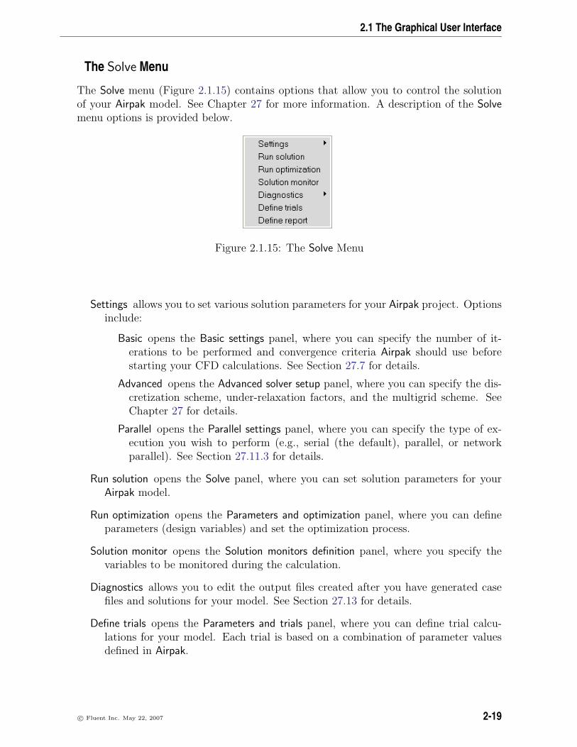
2.1 The Graphical User Interface
The Solve Menu
The Solve menu (Figure 2.1.15) contains options that allow you to control the solutionof your Airpak model. See Chapter 27 for more information. A description of the Solvemenu options is provided below.
Figure 2.1.15: The Solve Menu
Settings allows you to set various solution parameters for your Airpak project. Optionsinclude:
Basic opens the Basic settings panel, where you can specify the number of it-erations to be performed and convergence criteria Airpak should use beforestarting your CFD calculations. See Section 27.7 for details.
Advanced opens the Advanced solver setup panel, where you can specify the dis-cretization scheme, under-relaxation factors, and the multigrid scheme. SeeChapter 27 for details.
Parallel opens the Parallel settings panel, where you can specify the type of ex-ecution you wish to perform (e.g., serial (the default), parallel, or networkparallel). See Section 27.11.3 for details.
Run solution opens the Solve panel, where you can set solution parameters for yourAirpak model.
Run optimization opens the Parameters and optimization panel, where you can defineparameters (design variables) and set the optimization process.
Solution monitor opens the Solution monitors definition panel, where you specify thevariables to be monitored during the calculation.
Diagnostics allows you to edit the output files created after you have generated casefiles and solutions for your model. See Section 27.13 for details.
Define trials opens the Parameters and trials panel, where you can define trial calcu-lations for your model. Each trial is based on a combination of parameter valuesdefined in Airpak.
c© Fluent Inc. May 22, 2007 2-19

User Interface
Define report opens the Define summary report panel, where you can specify a summaryreport for a variable on any or all objects in your Airpak model.
2-20 c© Fluent Inc. May 22, 2007

2.1 The Graphical User Interface
The Post Menu
The Post menu (Figure 28.1.1) contains options that allow your to access Airpak’s post-processing objects. See Chapter 28 for more information. A description of the Post menuoptions is provided below.
Figure 2.1.16: The Post Menu
Object face allows you to display results on object faces in the model.
Plane cut allows you to display results on cross-sections of the model.
Isosurface allows you to display results on defined isosurfaces in the model.
Point allows you to create points and display results at points in the model.
Surface probe allows you to display results at a point on a postprocessing object thathas been created in the model.
Min/max locations allows you to display the location of the minimum and maximumvalues for postprocessed variables.
Convergence plot allows you to display the convergence history of the solution.
c© Fluent Inc. May 22, 2007 2-21

User Interface
Variation plot allows you to plot a variable along a line through the model.
History plot allows you to plot solution variable histories over time.
Trials plot allows you to plot solution variables at specified points across multiple trials.
Transient settings opens the Post-processing time panel, where you can set parametersfor transient simulations.
Load solution ID allows you to select a specific solution set to be examined.
Time average allows you to view the results of a time averaged (transient) problem asif it were steady-state.
Download RSF project opens the Download RSF project panel, where you can run anAirpak job using the Remote Simulation Facility (RSF) and download the resultsfor postprocessing in Airpak.
Postprocessing units opens the Postprocessing units panel, where you can choose theunits for different postprocessing variables.
Load post objects from file allows you to load postprocessing objects from a file.
Save post objects to file allows you to save postprocessing objects to a file.
Rescale vectors allows you to redisplay vectors drawn at their original sizes.
Create zoom-in model allows you to zoom in and define a region in your Airpak modeland save that region as a separate Airpak project.
The Report Menu
The Report menu (Figure 2.1.17) contains options for generating output concerning theresults of your Airpak model. See Chapter 29 for more information. A description of theReport menu options is provided below.
HTML report opens the HTML report panel, where you can customize your results andwrite out an HTML document that can be viewed in a web browser.
Solution overview allows you to view and create solution overview files.
View opens a File selection dialog box, where you can open a solution overviewfile (*.overview) in which summary data is stored for a particular solution.
Create opens a Version selection panel, where you can select a solution for whichto create an overview file. See Section 29.4 for details.
2-22 c© Fluent Inc. May 22, 2007

2.1 The Graphical User Interface
Figure 2.1.17: The Report Menu
Show optimization/param results opens an Optimization run panel, where you can viewall the function values, design variables, and the running times for each optimizationiteration, as well as the plots of the function values and design variables versusiteration number.
Summary report opens the Define summary report panel, where you can specify a sum-mary report for a variable on any or all objects in your Airpak model.
Point report opens the Define point report panel, where you can create a report for avariable at any point in your Airpak model.
Full report allows you to customize the report of your results.
Fan operating points allows you to create a report of the fan operating points for fansusing fan curves in your model.
Comfort level allows you to create a report of Indoor Air Quality (IAQ) and thermalcomfort level results.
ADPI report allows you to create a report of the Air Diffusion Performance Index(ADPI) for a specified region in your model.
The Windows Menu
The Windows menu contains the names of Airpak panels when one or more of them areopen. This feature is useful when you have many panels or toolbars open and you wishto quickly locate a specific toolbar or panel. An asterisk (*) to the left of a panel ortoolbar name indicates that the panel or toolbar is currently hidden. You can show orhide toolbars using the Available toolbars panel through the Edit toolbars option under theView menu. See Section 2.1.2 for more information about showing and hiding toolbarsusing the View menu.
c© Fluent Inc. May 22, 2007 2-23
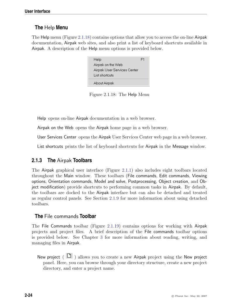
User Interface
The Help Menu
The Help menu (Figure 2.1.18) contains options that allow you to access the on-line Airpakdocumentation, Airpak web sites, and also print a list of keyboard shortcuts available inAirpak. A description of the Help menu options is provided below.
Figure 2.1.18: The Help Menu
Help opens on-line Airpak documentation in a web browser.
Airpak on the Web opens the Airpak home page in a web browser.
User Services Center opens the Airpak User Services Center web page in a web browser.
List shortcuts prints the list of keyboard shortcuts for Airpak in the Message window.
2.1.3 The Airpak Toolbars
The Airpak graphical user interface (Figure 2.1.1) also includes eight toolbars locatedthroughout the Main window. These toolbars (File commands, Edit commands, Viewingoptions, Orientation commands, Model and solve, Postprocessing, Object creation, and Ob-ject modification) provide shortcuts to performing common tasks in Airpak. By default,the toolbars are docked to the Airpak interface but can also be detached and treatedas regular control panels. See Section 2.1.9 for more information about using detachedtoolbars.
The File commands Toolbar
The File Commands toolbar (Figure 2.1.19) contains options for working with Airpakprojects and project files. A brief description of the File commands toolbar optionsis provided below. See Chapter 3 for more information about reading, writing, andmanaging files in Airpak.
New project ( ) allows you to create a new Airpak project using the New projectpanel. Here, you can browse through your directory structure, create a new projectdirectory, and enter a project name.
2-24 c© Fluent Inc. May 22, 2007

2.1 The Graphical User Interface
Figure 2.1.19: The File commands Toolbar
Open project ( ) allows you to open existing Airpak projects using the Open projectpanel. Here, you can browse through your directory structure, locate a projectdirectory, and either enter a project name, or specify an old project name from alist of recent projects. Additionally, you can specify a version name or number forthe project.
Save project ( ) saves the current Airpak project.
Print screen ( ) allows you to print a PostScript image of the Airpak model thatis displayed in the graphics window using the Print options panel. The inputs forthe Print options panel are similar to those in the Graphics file options panel. SeeSection 3.5 for details.
Create image file ( ) opens a Save image dialog that allows you to save your modeldisplayed in the graphics window to an image file. Supported file types include:PPM, GIF, JPEG, TIFF, VRML, and PS.
The Edit commands Toolbar
The Edit commands toolbar (Figure 2.1.20) contains options that allow you to performundo and redo operations in your Airpak model. A description of the Edit commandstoolbar options is provided below. See Chapter 7 for more information about editingobjects in Airpak.
Figure 2.1.20: The Edit commands Toolbar
Undo ( ) allows you to undo the last model operation you performed. Undo canbe used repeatedly to take you back to the first operation performed.
Redo ( ) allows you to redo one or more previously undone operations. This optionapplies only to operations undone by selecting the Undo option.
c© Fluent Inc. May 22, 2007 2-25
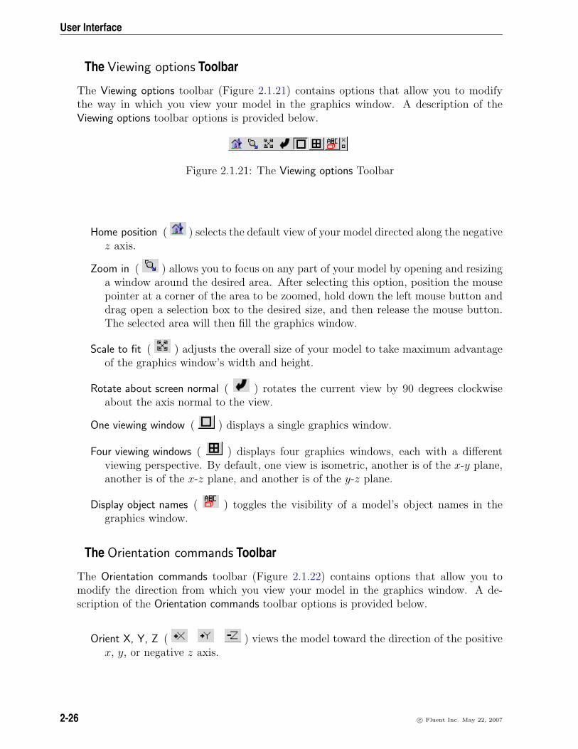
User Interface
The Viewing options Toolbar
The Viewing options toolbar (Figure 2.1.21) contains options that allow you to modifythe way in which you view your model in the graphics window. A description of theViewing options toolbar options is provided below.
Figure 2.1.21: The Viewing options Toolbar
Home position ( ) selects the default view of your model directed along the negativez axis.
Zoom in ( ) allows you to focus on any part of your model by opening and resizinga window around the desired area. After selecting this option, position the mousepointer at a corner of the area to be zoomed, hold down the left mouse button anddrag open a selection box to the desired size, and then release the mouse button.The selected area will then fill the graphics window.
Scale to fit ( ) adjusts the overall size of your model to take maximum advantageof the graphics window’s width and height.
Rotate about screen normal ( ) rotates the current view by 90 degrees clockwiseabout the axis normal to the view.
One viewing window ( ) displays a single graphics window.
Four viewing windows ( ) displays four graphics windows, each with a differentviewing perspective. By default, one view is isometric, another is of the x-y plane,another is of the x-z plane, and another is of the y-z plane.
Display object names ( ) toggles the visibility of a model’s object names in thegraphics window.
The Orientation commands Toolbar
The Orientation commands toolbar (Figure 2.1.22) contains options that allow you tomodify the direction from which you view your model in the graphics window. A de-scription of the Orientation commands toolbar options is provided below.
Orient X, Y, Z ( ) views the model toward the direction of the positivex, y, or negative z axis.
2-26 c© Fluent Inc. May 22, 2007

2.1 The Graphical User Interface
Figure 2.1.22: The Orientation commands Toolbar
Isometric view ( ) views the model from the direction of the vector equidistant toall three axes.
Reverse orientation ( ) views the model along the current view vector but from theopposite direction (i.e., rotated 180 degrees).
The Model and solve Toolbar
The Model and solve toolbar (Figure 2.1.23) contains options that allow you to generatea mesh, model radiation, check your model, and run a solution. A description of theModel and solve toolbar options is provided below.
Figure 2.1.23: The Model and solve Toolbar
Power and temperature limits ( ) opens the Power and temperature limit setup panel,where you can review or change the power of objects, as well as specify the tem-perature limits.
Generate mesh ( ) opens the Mesh control panel, where you can provide settings tocreate a mesh for your Airpak model. See Chapter 26 for more information aboutgenerating meshes.
Radiation ( ) opens the Form factors panel, where you can model radiation forspecific objects in your model. See Chapter 22 for more information about radiationmodels in Airpak.
Check model ( ) performs a check to test the model for problems in the design.See Section 7.3.7 for details.
Run solution ( ) opens the Solve panel, where you can set solution parameters foryour Airpak model.
Run optimization ( ) opens the Parameters and optimization panel, where you candefine parameters (design variables) and set the optimization process.
c© Fluent Inc. May 22, 2007 2-27

User Interface
The Postprocessing Toolbar
The Postprocessing toolbar (Figure 28.1.2) contains options that allow you to examineyour results using Airpak’s postprocessing objects. A description of the Postprocessingtoolbar options is provided below. See Chapter 28 for more information about postpro-cessing.
Figure 2.1.24: The Postprocessing Toolbar
Object face ( ) allows you to display results on object faces in the model.
Plane cut ( ) allows you to display results on cross-sections of the model.
Isosurface ( ) allows you to display results on defined isosurfaces in the model.
Point ( ) allows you to display results at points in the model.
Surface probe ( ) allows you to display results at a point on a surface in the model.
Variation plot ( ) allows you to plot a variable along a line through the model.
History plot ( ) allows you to plot solution variable histories over time.
Trials plot ( ) allows you to plot trial solution variables.
Transient settings ( ) opens the Post-processing time panel, where you can setparameters for transient simulations.
Load solution ID ( ) allows you to select a specific solution set to be examined.
Time average ( ) allows you to view the results of a time averaged (transient)problem as if it were steady-state.
Download RSF project ( ) opens the Download RSF project panel, where you canrun an Airpak job using the Remote Simulation Facility (RSF) and download theresults for postprocessing in Airpak.
Summary report ( ) opens the Define summary report panel, where you can specifya summary report for a variable on any or all objects in your Airpak model.
2-28 c© Fluent Inc. May 22, 2007

2.1 The Graphical User Interface
The Object creation Toolbar
The Object creation toolbar (Figure 7.1.1) contains options that allow you to add objectsto your Airpak model. A description of the Object creation toolbar options is providedbelow. Unless otherwise noted, all objects are created in the center of the correspondingmodel room.
Figure 2.1.25: The Object creation Toolbar
Create blocks ( ) allows you to create a block object. See Chapter 8 for details.
Create fans ( ) allows you to create a fan object. See Chapter 9 for details.
Create vents ( ) allows you to create a vent object. See Chapter 10 for details.
Create openings ( ) allows you to create an opening object. See Chapter 11 fordetails.
Create persons ( ) allows you to create a person object. See Chapter 12 for details.
Create walls ( ) allows you to create a wall object. See Chapter 13 for details.
Create partitions ( ) allows you to create a partition object. See Chapter 14 fordetails.
Create sources ( ) allows you to create a source object. See Chapter 15 for details.
c© Fluent Inc. May 22, 2007 2-29

User Interface
Create resistances ( ) allows you to create a 3D resistance object. See Chapter 16for details.
Create heat exchangers ( ) allows you to create a heat exchanger object. SeeChapter 17 for details.
Create hoods ( ) allows you to create a hood object. See Chapter 18 for details.
Create assemblies ( ) allows you to create an assembly object at the origin of thegraphics window. See Chapter 7 for details.
Create wires ( ) allows you to create a wire object. See Chapter 19 for details.
Create materials ( ) allows you to create a materials node for the model in theModel manager window. See Chapter 7 for details.
The Object modification Toolbar
The Object modification toolbar (Figure 2.1.26) contains options that allow you to edit,delete, move, copy, or align an object in your Airpak model. A description of the Objectmodification toolbar options is provided below. See Chapter 7 for details about modifyingobjects in Airpak.
Figure 2.1.26: The Object modification Toolbar
Edit object ( ) opens an object-specific Edit window, where you can set variousobject properties.
Delete object ( ) removes the object from the model.
2-30 c© Fluent Inc. May 22, 2007

2.1 The Graphical User Interface
Move object ( ) opens an object-specific Move panel, where you can scale, rotate,translate, or mirror an object.
Copy object ( ) opens an object-specific Copy panel, where you can create a copyof an object and then scale, rotate, translate, or mirror the copied object.
Align and morph faces ( ) aligns the faces of two objects.
Align and morph edges ( ) aligns the edges of two objects.
Align and morph vertices ( ) aligns the vertices of two objects.
Align object centers ( ) aligns the centers of two objects.
Align face centers ( ) aligns the centers of the faces of two objects.
Morph faces ( ) matches the faces of two objects.
Morph edges ( ) matches the edges of two objects.
2.1.4 The Model manager Window
The Airpak Model manager window (Figure 2.1.27) provides a localized area for defin-ing your Airpak model and contains a project-specific listing of problem and solutionparameters.
The Model manager window is presented in a tree-like structure with expandable andcollapsible tree nodes that show or hide relevant tree items. To expand a tree node, use
the left mouse button to click on the icon on the left hand side of the tree. Tocollapse a tree node, click on the icon.
You can edit and manage your Airpak project from within the Model manager windowusing the mouse. For example, you can select multiple objects, edit project parameters,add groups within groups, break apart assemblies, or edit objects, by clicking and drag-ging objects. In addition, the Model manager window includes a context menu, accessibleby right-clicking the mouse, that allows you to easily manipulate your Airpak model. SeeSection 2.2.2 for more information on using the mouse in the Model manager window.
An Airpak project is organized in the Model manager window using six different categories:
Problem setup ( ) allows you to set basic problem parameters, set the project title,and define local coordinate systems. Options include:
Basic parameters ( ) opens the Basic parameters panel, where you can specifyparameters for the current Airpak model. See Section 6.4 for details.
c© Fluent Inc. May 22, 2007 2-31

User Interface
Figure 2.1.27: An Example of the Model manager Window
2-32 c© Fluent Inc. May 22, 2007

2.1 The Graphical User Interface
Title/notes ( ) opens the Title/notes panel, where you can enter a title andnotes for the current Airpak model. panel, where you can create local coor-dinate systems that can be used in your model other than the Airpak globalcoordinate system with an origin of (0, 0, 0). The origins of the local co-ordinate systems are specified with an offset from the origin of the globalcoordinate system. See Section 7.3.7 for details.
Solution settings ( ) allows you to set Airpak solution parameters. Options include:
Basic settings ( ) opens the Basic settings panel, where you can specify thenumber of iterations to be performed and convergence criteria Airpak shoulduse before starting your CFD calculations. See Section 27.7 for details.
Parallel settings ( ) opens the Parallel settings panel, where you can specifythe type of execution you wish to perform (e.g., serial (the default), parallel,or network parallel). See Section 27.11.3 for details.
Advanced settings ( ) opens the Advanced solver setup panel, where you canspecify the discretization scheme, under-relaxation factors, and the multigridscheme. See Chapter 27 for details.
Libraries ( ) lists the libraries used in your Airpak project. By default, a Main libraryexists in your Airpak project that contains materials (fluids, solids, and surfaces),fan objects, and other complex objects. See Section 7.7 for details.
Groups ( ) lists any groups of objects in the current Airpak project. See Section 7.6for details about grouping objects.
Post-processing ( ) lists any postprocessing objects in the current Airpak project.See Chapter 28 for details about postprocessing in Airpak.
Points ( ) lists any point monitoring objects in the current Airpak project. SeeSection 27.8.1 for details about point monitors.
Trash ( ) lists any objects that have been deleted from the Airpak model. Anyitems in the Trash node will only be available for the current Airpak session.
Inactive ( ) lists any objects that have been made inactive in the Airpak model.
Model ( ) lists all active objects and materials for the Airpak project.
2.1.5 Graphics Windows
Displaying graphics is an important aspect of the Airpak graphical user interface. Thereare two types of graphical displays in Airpak: a graphics window (or Model Display win-dow) and a graphics display and control window.
c© Fluent Inc. May 22, 2007 2-33

User Interface
The graphics window (or Model Display window) displays your Airpak model and takesup most of the Main window (Figure 2.1.1). It is the working space for building andmanipulating your model. The graphics window contains only a graphical display ofyour model; it does not contain any control features.
At the lower left corner of the graphics window is a three-dimensional coordinate axessystem, which indicates the current orientation of your model. The axis that is closestto your line of sight is displayed in a diamond shape. As you rotate your model, the axesrotate as well, and vice versa. You can manipulate objects in the graphics window usingthe mouse; see Section 2.2.4 for details.
The other type of graphics window you can encounter in Airpak is a graphics displayand control window, which provides graphics display as well as control features (anexample is shown in Figure 2.1.28). These types of windows open during specific model-building and simulation processes. For example, if you are displaying residuals while asolution is being calculated, the Solution residuals window will appear on the screen asshown in Figure 2.1.28. In addition to the graphics, a set of control features is provided,which are located at the bottom of the window. These control features are described inSection 27.12.2.
2-34 c© Fluent Inc. May 22, 2007

2.1 The Graphical User Interface
Figure 2.1.28: Example of a Graphics Window With Controls
c© Fluent Inc. May 22, 2007 2-35

User Interface
Adding Annotations to the Graphics Window
You can add annotations (e.g., labels and arrows) to the graphics window using theAnnotations panel. To open the Annotations panel, select the Annotations option in theEdit menu.
Edit−→Annotations
Figure 2.1.29: The Annotations Panel
The following options are available for annotations:
Title includes the job title in the graphics window.
Date includes the current date in the graphics window.
Logo includes the Airpak logo in the graphics window.
Arrows includes arrows in the graphics window. You can Add arrows, Edit arrows,Remove one arrow at a time, or Clear all arrows. Airpak displays messages in thegraphics window regarding positioning and modifying arrows.
2-36 c© Fluent Inc. May 22, 2007

2.1 The Graphical User Interface
Text includes alphanumeric notations in the graphics window. You can Add text, Edittext, Remove one text annotation at a time, or Clear all text annotations. Airpakdisplays messages in the graphics window regarding positioning and modifying textannotations.
Lines includes lines in the graphics window. You can Add lines, Edit lines, Remove oneline at a time, or Clear all lines. Airpak displays messages in the graphics windowregarding positioning and modifying lines.
Markers includes markers in the graphics window. You can Add markers, Edit markers,Remove one marker at a time, or Clear all markers. Airpak displays messages in thegraphics window regarding positioning and modifying markers.
For new annotations defines the Color, Line width, and Point size for new annotations.The defaults are white for Color, 1 for Line width, and 5 for Point size.
The annotations will remain in the graphics window for the current session until you turnthem off in the Annotations panel. Annotations are saved when you save a job file. Youcan add annotations to your image files (see Section 3.5 for details about image files).
2.1.6 The Message Window
The Message window (Figure 2.1.30) is located below the graphics window. Airpak com-municates with you through its Message window. It is used to display informative mes-sages, such as those relating to meshing or solution procedures, as well as error messagesand instructions. Airpak saves all information that is written to the Message window inmemory. You can review this information at any time by using the scroll bar on theright-hand side of the Message window. To instruct Airpak to display more detailed mes-sages related to the meshing and solution procedures, select the Verbose option in theMessage window.
Figure 2.1.30: Sample Message Window
To write this information to a file, follow the steps below.
c© Fluent Inc. May 22, 2007 2-37

User Interface
1. Click on the Save push button in the Message window. A Save log dialog box ap-pears. The default name (messages.01.txt) for the saved information will appearin the File name field at the bottom of the Save log dialog box.
2. To specify a different file name, type it in the text field.
3. Click the Save button in the Save log dialog box to save the file. Click the Cancelbutton to cancel the procedure.
You can save the file multiple times in the same Airpak session.
You can also direct Airpak to log all information that is reported in the Message windowto a log file. To do this, follow the steps below.
1. Select the Log option in the Message window (Figure 2.1.30). A File selection dialogbox appears. The default name (messages.log) for the log file will appear in theFile name field at the bottom of the File selection dialog box.
2. To specify a different filename, type it in the text field.
3. Click the Open button in the File selection dialog box to start the log file. Click theCancel button to cancel the procedure.
2.1.7 The Edit Window
The Edit window is located in the lower right corner of the screen below the graphicswindow. This window displays geometric data and other general properties for a selectedobject. The layout of this window and the data displayed in this window change depend-ing on the currently selected object in the graphics window. For example, when you areconstructing a fan, the Edit window becomes the fan Edit window. An example of theEdit window is shown in Figure 2.1.31.
Figure 2.1.31: Sample Edit Window
2-38 c© Fluent Inc. May 22, 2007

2.1 The Graphical User Interface
2.1.8 File Selection Dialog Boxes
File selection dialog boxes enable you to choose a file for reading or writing. You can usethem to look at your system directories and select a file.
Note that the appearance of the file selection dialog box will not always be the same. Theversion shown in Figure 2.1.32 will appear in many cases. If you are saving a project, theversion shown in Figure 2.1.33 will appear. If you are opening a project, merging twoprojects, or loading an external assembly, a version similar to that shown in Figures 2.1.34and 2.1.35 will appear.
Figure 2.1.32: The File selection Dialog Box
The steps for file selection are as follows:
1. (Windows systems only) In the Drive drop-down list, select the drive on your systemthat contains the file.
2. Go to the appropriate directory. You can do this in three different ways:
• Select or enter the desired directory in the Directory name field/drop-down list.You can enter the full pathname (beginning with a / character on a UNIXsystem or a drive letter on Windows) or a pathname relative to the directoryin which Airpak was started. Be sure to include the final / character in thepathname. Note that you can also move one level up a directory tree using
the button.
• Double-click on a directory, and then a subdirectory, etc., in the directorieslist until you reach the directory you want. Note that the directories list isalways located under the Directory name field/drop-down list.
c© Fluent Inc. May 22, 2007 2-39

User Interface
Figure 2.1.33: The Save project Panel Showing the File Selection Dialog
Figure 2.1.34: The Open project Panel Showing the File Selection Dialog andthe Preview Tab
2-40 c© Fluent Inc. May 22, 2007

2.1 The Graphical User Interface
Figure 2.1.35: The Open project Panel Showing the File Selection Dialog andthe Information Tab
• Most file selection dialogs contain a button that allow you to create a new
directory ( ) at the top of the panel. If you want to create a new directory,
for example, to save a job file into a new directory, you can click thebutton. Airpak will prompt you for the name of the new directory. Enter aname in the New directory name text entry box, and then click Done. Airpakwill create a new directory with the specified name and then open the newdirectory.
3. Specify the file name, if necessary, by selecting it in the listing of files and directories,or by entering the name of the file in the File name text entry box. The name ofthis text entry box will change depending on the type of file you are selecting (e.g.,Project in the Save project panel).
4. (project files only) You can choose from a number of previously opened Airpakproject files in the Recent projects drop-down list.
5. (project files only) Select the version of the job file in the Versions drop-downlist (e.g., in the Open project panel shown in Figure 2.1.34). This list displays theavailable versions for the project file selected. The version listing is also available inthe Information tab of some file selection dialogs. For example, if you run a projectwith a project ID of job01, Airpak will save a model file called job01.model. If,for example, you then change the material properties specified for a block in yourmodel, and give this project an ID of job02, Airpak will save a model file calledjob02.model. These files are all saved in the same directory. When you selectthe directory in the Directory list, all the different versions of the project in thatdirectory will be displayed in the Versions drop-down list.
c© Fluent Inc. May 22, 2007 2-41

User Interface
6. (project files only) To apply the settings you specified under Options in the Pref-erences panel (see Section 6.3) from the previous time you worked on the project,turn on the Apply user preferences from project option.
7. (project files only) Title, Versions, and Notes fields will appear in the Information tabof some of the file selection dialogs (e.g., Figure 2.1.35). In addition, the Previewtab (e.g., Figure 2.1.34) may contain a picture of the model if a picture has beensaved. These items are described below.
• Title displays the title of the job file selected. See Section 6.2.1 for informationon adding a title to a job.
• Notes displays any notes related to the job file selected. See Section 6.2.1 forinformation on adding notes to a job.
• A picture of the geometry of the model will be displayed if you selected theSave picture file option in the Save project panel when you saved the project.See Section 3.4 for more information on the Save picture file option.
8. In some of the file selection dialogs there are other options that you can select, forexample, on the right-hand side of the Save project panel (Figure 2.1.33). Theseoptions are described in the section related to the use of that particular panel, forexample, the options in the Save project panel are described in Section 3.4.
9. Click on the Save button to read or write the specified file. Shortcuts for this stepare as follows:
• If your file appears in the listing of files and directories, double-click on itinstead of just selecting it. This will automatically activate the Open buttonfor opening files, the Create button for creating projects, or the Save buttonfor saving files.
• If you entered the name of the file in the File name text entry box, you canpress the <Enter> key instead of clicking on the Open button for opening files,the Create button for creating projects, or the Save button for saving files.
2.1.9 Control Panels
Control panels, which are used to perform input tasks, are another major componentof the GUI. They are displayed in a separate window, and are invoked by means of ahigher-level function selection. Figure 2.1.36 shows an example of a control panel.
Working with a panel is similar to filling out a form. You provide input data to thepanel’s controls. Once you have finished entering data, you either apply the changes by“submitting” the form, or cancel the form. Clicking on the Accept push button acceptsany changes you have made to the panel, and closes the panel. Clicking on the Resetbutton undoes all the changes you have made in the panel and restores all items in the
2-42 c© Fluent Inc. May 22, 2007

2.1 The Graphical User Interface
Figure 2.1.36: Example of a Control Panel
panel to their original states. Cancel closes the panel and ignores any changes made tothe panel.
Each panel is unique, and uses a variety of input controls that are described below.
Push Button
A push button is a rectangular-shaped button that performs a function indicated by thebutton label. To activate a push button, place the mouse pointer over the push buttonand “click” the left mouse button. A “click” is one press and release of the mouse button.When push buttons are located on a menu bar, they usually cause a submenu to appear,or a panel to be displayed.
Check Box
A check box is a square-shaped button that is used to turn on or off an item or actionindicated by the check box label. Click the left mouse button on the check box to switchthe state.
c© Fluent Inc. May 22, 2007 2-43

User Interface
Radio Button
Radio buttons are diamond-shaped buttons that are located on a menu bar or panel.They are a set of mutually exclusive options that allow only one to be set in the “on”position at a time. When you click the left mouse button on a radio button, it will beturned on, and all others will be turned “off”.
Text Entry
A text entry allows you to type text input. It will often have a label associated with it toindicate what the entry is for. Click the left mouse button on the text entry field to inputtext from the keyboard. If the text input overflows the field, you can scroll backwardor forward in the field by pressing and holding down the middle mouse button. Youcan delete characters in the text entry field using the <Del> or <Back Space> key. Inaddition, you can double-click on the text entry with the left mouse button to highlightthe entire field, and type the new entry.
Real Number Entry
A real number entry is similar to a text entry except it allows only real numbers to beentered (e.g., 10, -10.538, 50000.45, or 5.e-4).
2-44 c© Fluent Inc. May 22, 2007
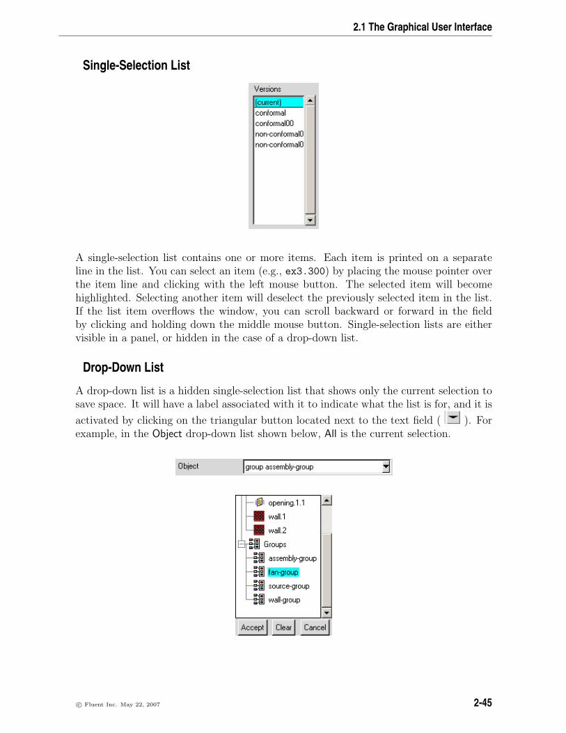
2.1 The Graphical User Interface
Single-Selection List
A single-selection list contains one or more items. Each item is printed on a separateline in the list. You can select an item (e.g., ex3.300) by placing the mouse pointer overthe item line and clicking with the left mouse button. The selected item will becomehighlighted. Selecting another item will deselect the previously selected item in the list.If the list item overflows the window, you can scroll backward or forward in the fieldby clicking and holding down the middle mouse button. Single-selection lists are eithervisible in a panel, or hidden in the case of a drop-down list.
Drop-Down List
A drop-down list is a hidden single-selection list that shows only the current selection tosave space. It will have a label associated with it to indicate what the list is for, and it is
activated by clicking on the triangular button located next to the text field ( ). Forexample, in the Object drop-down list shown below, All is the current selection.
c© Fluent Inc. May 22, 2007 2-45

User Interface
When you want to change the selection (e.g., from assembly-group to fan-group), followthe steps below:
1. Click on the button located next to the text field to display the list.
2. Place the mouse pointer over the new list item (e.g., fan-group). If the item is notvisible, you can use the scroll bar to find it.
3. Click the left mouse button on the item to make the new selection. The list willclose automatically, and the new selection will then be displayed.
If you want to abort the selection process while the list is displayed, you can move thepointer anywhere outside the list and click the left mouse button, or click Cancel.
Scale
The scale is used to select a value from a predefined range by moving a slider. Thenumber shows the current value. To change the value, follow the steps below:
1. Place the pointer over the slider.
2. Press and hold down the left mouse button.
3. Move the pointer along the slider bar to change the value.
4. Release the left mouse button.
Tabs
Many of the Airpak panels (e.g., object editing panels) include tabbed regions that sepa-rate different categories of input fields. For instance, the Walls panel includes four tabs:Info, Geometry, Properties, and Notes, as seen in Figure 2.1.37. Here, you can access theappropriate category for the object, in this case, a wall. To display the contents of aparticular tab, select the tab label with the left mouse button.
Many tabbed panels have the following types of tab categories:
Info displays general information about the object such as its name, its group, andother display properties.
Geometry displays geometric information such as its shape, its plane, and its coordi-nates.
2-46 c© Fluent Inc. May 22, 2007

2.1 The Graphical User Interface
Figure 2.1.37: An Example of a Tabbed Panel
Properties provides access to the object’s material and thermal properties.
Notes provides an area for you to leave notations about the object.
Note that some object and macro panels include different tabs that are based on theproperties of the object.
Floating Toolbars
Most of the Airpak toolbars can be detached from the Main window and exist as floatingtoolbars that can be moved to any position in the window. Floating toolbars are identified
by two small buttons in the upper right hand corner of the toolbar ( ).
You can detach a toolbar, by clicking on the button. To move the detached toolbar,select the title bar and drag the toolbar to a new position in the Main window. To resizea detached toolbar, click and drag the edge of the toolbar to the desired position usingthe left mouse button.
c© Fluent Inc. May 22, 2007 2-47

User Interface
Figure 2.1.38: Floating Toolbars
To hide an attached toolbar entirely from view in the Airpak graphical interface, click on
the button.
You can re-attach a floating toolbar to the Airpak interface, by clicking on the buttonin the upper right hand corner of the floating toolbar. To hide a floating toolbar entirely
from view in the Airpak graphical interface, select the icon in the upper right handcorner of the floating toolbar.
Whether attached or detached, you can retrieve a hidden toolbar using the Windows menuor selecting the Edit toolbars option in the View menu and using the Available toolbarspanel.
View−→Edit toolbars
2.1.10 Accessing On-line Help
There are three types of help available in Airpak: on-line help, bubble help, and context-specific help. On-line help provides access to on-line versions of the Airpak manuals.Bubble help provides a brief explanation of the function performed by items in the Mainwindow, the Message window, the Edit window, the Model manager window, the varioustoolbars, and control panels. Context-specific help provides specific information for apanel or window.
On-Line Help
To invoke the on-line help system, select the Help option in the Help menu. The HTMLversion of the Airpak User’s Guide will be displayed in your web browser. Airpak will au-tomatically launch your web browser. You can access information in the manual throughthe hyperlinks in the table of contents and index. To access the Airpak Tutorial Guide,click the Return to Home button at the top of the page and then select the HTML version
2-48 c© Fluent Inc. May 22, 2007

2.2 Using the Mouse
of the Tutorial Guide from the Airpak documentation home page. See Section 1.6 forinformation on using the on-line manuals.
Bubble Help
Bubble help (i.e., tool tips) is available for radio buttons, push buttons, and togglebuttons in the Main window, the Message window, the Edit window, the toolbars, andcontrol panels. To use bubble help, hold the mouse pointer over an item for a fewseconds. A bubble will appear giving a brief description of the function of the item. Youcan disable the bubble help, as described in Section 6.3.
Context-Specific Help
To use context-specific help, move the mouse pointer to any location within the panelyou require help for, and press the F1 key. Airpak will automatically launch your webbrowser, open the appropriate on-line document, and locate the heading or figure withinthe document that relates to the panel in question.
2.2 Using the Mouse
The mouse is used as the primary means of interacting with the graphical user interface(GUI) to access Airpak’s functionality. To take full advantage of the functionality availablein Airpak, you will need a three-button mouse.
The mouse can be used to provide inputs to control panels, display control panels, accessobjects in the Model manager window, as well as manipulate objects in the graphicswindow.
2.2.1 Controlling Panel Inputs
The left mouse button is used to control panel inputs in the following ways:
• Executing selector button functions (e.g., push buttons, radio buttons, toggle but-tons)
• Highlighting items in a list
• Enabling a text field for typing
In addition, the middle mouse button allows you to drag into view text entries or listitems that overflow the field.
c© Fluent Inc. May 22, 2007 2-49

User Interface
2.2.2 Using the Mouse in the Model manager Window
The left mouse button is used in the Model manager window in the following ways:
• Opening and closing tree nodes by clicking on the or icons to the left ofthe tree node name.
• Selecting node items by clicking on the item in the Model manager window. Theitem is highlighted when it is selected.
• Dragging and dropping items to other locations in the tree. To do this, hold downthe left mouse button on an item (e.g., in the Group, Model, or Materials nodes),drag the item to another area of the tree, and drop the item into the tree byreleasing the left mouse button.
• Selecting and operating on multiple items in the Model manager window by holdingdown the <Control> key while you select items. To select a succession of items(e.g., fan.1, fan.2,..., fan.10) select the first item (e.g.,fan.1), hold down the <Shift>key and select the last item (e.g.,fan.10). All items between the first item and thelast item will become selected in the Model manager window.
• Double-clicking on certain tree items will open a control panel for additional input(e.g., to set project parameters and options, or edit object properties).
In addition, there are context menus available in the Airpak Model manager window, asdescribed in the next section.
2.2.3 Using the Context Menus in the Model manager Window
Airpak includes a context menu that you can access by holding down the right mousebutton on certain objects that are selected in the Model manager window. The contextmenu is useful in the Model manager window when you want to quickly perform commontasks on the objects in your model.
The Main library Node Context Menu
When the Main library node is selected, the context menu includes the following options:
Edit info opens the Library name and info panel, where you can view and edit the libraryname and information fields. See Section 7.7 for details.
Paste from clipboard allows you to add objects or materials to the Airpak library thatyou have placed in the clipboard. See page 2-59 for more information about theclipboard.
Refresh updates the library if any changes (additions or subtractions) have been madeto the library repository.
2-50 c© Fluent Inc. May 22, 2007

2.2 Using the Mouse
The Groups Node Context Menus
When the Groups node is selected, the context menu includes the following options:
Create allows you to name a new group and then add the new group as an item underthe Groups node.
When an individual group node is selected under the Groups node (e.g., group.1), thecontext menu includes the following options:
Paste from clipboard pastes the group from the clipboard to your model. See page 2-59for more information about the clipboard.
Properties opens the Group parameters panel, where you can set color, line width, andshading properties for objects in the group.
Rename allows you to rename the group.
Delete moves the group to the Trash node.
Add allows you to add objects to a group by selecting a point or region on the screenor choosing an object name or pattern.
Remove allows you to remove objects from a group by selecting a point or region onthe screen or choosing an object name or pattern.
Copy group opens the group Copy panel, where you can copy a group then scale, rotate,translate, or mirror the copied group.
Move group opens the group Move panel, where you can scale, rotate, translate, ormirror a group.
Edit objects opens the object Edit window, where you can edit object properties if allobjects in the group are of the same type.
Visible toggles the display of the group in the graphics window.
Activate all activates all inactive objects in the group.
Deactivate all deactivates all active objects in the group.
Delete all deletes all objects in the group
Total volume prints the total volume of all objects from the group in the Messagewindow.
Total area prints the total area of all objects from the group in the Message window.
c© Fluent Inc. May 22, 2007 2-51

User Interface
Create assembly creates an assembly out of the group. See Section 7.8 for details.
Copy params applies the parameters of the selected object to all objects of the sametype in the selected group.
Save as project allows you to save the selected group as a separate Airpak project.
See Section 7.6 for details about grouping objects.
When an individual item in a Groups node is selected (e.g., block.1), the context menuincludes the following options:
Add to clipboard copies the item to the clipboard. See page 2-59 for more informationabout the clipboard.
Paste from clipboard pastes the item from the clipboard to your model. See page 2-59for more information about the clipboard.
Rename allows you to rename the item.
Copy object allows you to copy the selected object.
Move object allows you to move the selected object.
Edit object allows you to edit the properties of the item.
Delete moves the item to the Trash node.
Create assembly allows you to create an assembly from the selected item.
Create group allows you to create a group from the selected item.
Active allows you to toggle the item’s activity.
Visible allows you to toggle the item’s visibility. Hidden objects appear in the Modelmanager window as grayed out items and are not visible in the graphics window.This allows you to view and edit portions of your model while hiding the rest.
Total volume prints the total volume of selected objects in the Message window.
Total area prints the total area of selected objects in the Message window.
Create monitor point allows you to create monitor points for selected objects. Thiswill also copy the selected objects from the Model node into the Points node. SeeSection 27.8.1 for more information on object monitor points.
Edit mesh parameters opens up the Per-object parameters panel, where you can reviewand define meshing parameters specific to the selected object. See Section 26.6.1for more information on defining object-specific meshing parameters.
2-52 c© Fluent Inc. May 22, 2007

2.2 Using the Mouse
Create object face allows you to create object faces for selected objects. Newly createdobject faces will show up under the Post-processing node. See Section 28.2.4 for moreinformation on defining object faces.
Remove from group allows you to remove the object from the group. This optionappears in the context menu only for selected objects under the Groups node.
See Chapter 7 for more information about editing objects and groups of objects.
The Post-processing Node Context Menu
When an item in the Post-processing node is selected, the context menu includes thefollowing options:
Active allows you to toggle the postprocessing object’s activity. If this option is turnedoff, the postprocessing object is placed under the Inactive node.
Edit allows you to edit the postprocessing object.
Delete moves the postprocessing object to the Trash node.
See Chapter 28 for more information about postprocessing in Airpak.
The Points Node Context Menus
When the Points node is selected, the context menu includes the following option:
Create at location displays the Point panel, where you can define the location of solu-tion monitor points. See Section 27.8.1 for details.
Paste from clipboard allows you to add objects or materials to the Airpak library thatyou have placed in the clipboard. See page 2-59 for more information about theclipboard.
When an item in the Points node is selected, the context menu includes the followingoptions (see Section 27.8.1):
Edit info displays the Point panel, where you can monitor the temperature, pressure,and velocity parameters at a central point within an object.
Move displays the Move point panel, where you can specify a new coordinate locationfor an existing monitor point.
Copy displays the Copy point panel, where you can specify parameters for copying anexisting monitor point.
Delete deletes the monitor point.
c© Fluent Inc. May 22, 2007 2-53

User Interface
The Trash Node Context Menus
When the Trash node is selected, the context menu includes the following options:
Paste from clipboard empties the contents of the clipboard into the Trash node. Seepage 2-59 for more information about the clipboard.
Empty trash deletes the contents of the Trash node completely from the Airpak project.
When an item in the Trash node is selected, the context menu includes the followingoption:
Undelete allows you to add the deleted object back to your model.
The Inactive Node Context Menu
When an item in the Inactive node is selected, the context menu includes the followingoptions:
Add to clipboard copies the item to the clipboard. See page 2-59 for more informationabout the clipboard.
Paste from clipboard pastes the item from the clipboard to your model. See page 2-59for more information about the clipboard.
Rename allows you to rename the item.
Copy object allows you to copy the selected object.
Move object allows you to move the selected object.
Edit object allows you to edit the properties of the item.
Delete moves the item to the Trash node.
Create assembly allows you to create an assembly from the selected item.
Create group allows you to create a group from the selected item.
Active allows you to toggle the item’s activity.
Visible allows you to toggle the item’s visibility. Hidden objects appear in the Modelmanager window as grayed-out items and are not visible in the graphics window.This allows you to view and edit portions of your model while hiding the rest.
Total volume prints the total volume of selected objects in the Message window.
2-54 c© Fluent Inc. May 22, 2007

2.2 Using the Mouse
Total area prints the total area of selected objects in the Message window.
Create monitor point allows you to create monitor points for selected objects. Thiswill also copy the selected objects from the Model node into the Points node. SeeSection 27.8.1 for more information on object monitor points.
Edit mesh parameters opens up the Per-object parameters panel, where you can reviewand define meshing parameters specific to the selected object. See Section 26.6.1for more information on defining object-specific meshing parameters.
Create object face allows you to create object faces for selected objects. Newly createdobject faces will show up under the Post-processing node. See Section 28.2.4 for moreinformation on defining object faces.
Remove from group allows you to remove the object from the group. This optionappears in the context menu only for selected objects under the Groups node.
The Model Node Context Menus
When the Model node is selected, the context menu includes the following options:
Paste from clipboard empties the contents of the clipboard into your model. See page2-59 for more information about the clipboard.
Create allows you to add an Airpak object (e.g., block, fan, wire, etc.) to your model.
Merge project allows you to merge an existing project with your current project usingthe Merge project panel.
Load assembly allows you to load an assembly as another Airpak project using the Loadproject panel.
When an item in the Model node is selected (with the exception of the Room, the Materialsnode, and any assemblies), the context menu includes the following options:
Add to clipboard copies the item to the clipboard. See page 2-59 for more informationabout the clipboard.
Paste from clipboard pastes the item from the clipboard to your model. See page 2-59for more information about the clipboard.
Rename allows you to rename the item.
Copy object allows you to copy the selected object.
Move object allows you to move the selected object.
c© Fluent Inc. May 22, 2007 2-55

User Interface
Edit object allows you to edit the properties of the item.
Delete moves the item to the Trash node.
Create assembly allows you to create an assembly from the selected item.
Create group allows you to create a group from the selected item.
Active allows you to toggle the item’s activity.
Visible allows you to toggle the item’s visibility. Hidden objects appear in the Modelmanager window as grayed out items and are not visible in the graphics window.This allows you to view and edit portions of your model while hiding the rest.
Total volume prints the total volume of selected objects in the Message window.
Total area prints the total area of selected objects in the Message window.
Create monitor point allows you to create monitor points for selected objects. Thiswill also copy the selected objects from the Model node into the Points node. SeeSection 27.8.1 for more information on object monitor points.
Edit mesh parameters opens up the Per-object parameters panel, where you can reviewand define meshing parameters specific to the selected object. See Section 26.6.1for more information on defining object-specific meshing parameters.
Create object face allows you to create object faces for selected objects. Newly createdobject faces will show up under the Post-processing node. See Section 28.2.4 for moreinformation on defining object faces.
Remove from group allows you to remove the object from the group. This optionappears in the context menu only for selected objects under the Groups node.
See Chapter 7 for more information about adding objects and assemblies to your model,as well as about editing objects and groups of objects.
The Room Context Menu
When the Room in the Model node is selected, the context menu includes the followingoptions:
Add to clipboard copies the item to the clipboard. See page 2-59 for more informationabout the clipboard.
Paste from clipboard pastes the item from the clipboard to your model. See page 2-59for more information about the clipboard.
Rename allows you to rename the item.
2-56 c© Fluent Inc. May 22, 2007

2.2 Using the Mouse
Move object allows you to move the selected object.
Edit object allows you to edit the properties of the item.
Visible allows you to toggle the item’s visibility. Hidden objects appear in the Modelmanager window as grayed out items and are not visible in the graphics window.This allows you to view and edit portions of your model while hiding the rest.
Total volume prints the total volume of the selected object in the Message window.
Total area prints the total area of the selected object in the Message window.
The Materials Node Context Menu
When an item in the Materials node is selected, the context menu includes the followingoptions:
Add to clipboard copies the item to the clipboard. See page 2-59 for more informationabout the clipboard.
Copy material copies the item and adds it to your Airpak model.
Rename allows you to rename the item.
Edit allows you to edit the properties of the item.
Delete moves the material item to the Trash node.
See Section 7.7 for more information about materials.
The Assembly Node Context Menu
When an assembly node is selected, the context menu includes the following options:
Add to clipboard copies the item to the clipboard. See page 2-59 for more informationabout the clipboard.
Paste from clipboard pastes the item from the clipboard to your model. See page 2-59for more information about the clipboard.
Create allows you to create another Airpak object (e.g., block, fan, etc.) and adds itto the assembly.
Merge project allows you to merge an existing project with your current project usingthe Merge project panel. See Chapter 3 for more details.
c© Fluent Inc. May 22, 2007 2-57

User Interface
Load assembly allows you to load an assembly as another Airpak project using the Loadproject panel.
Save as project saves the assembly as an Airpak project.
View separately allows you to move the assembly item up to the level of the Modelnode in the Model manager window.
Rename allows you to rename the assembly item.
Copy object allows you to copy the selected assembly object.
Move object allows you to move the selected assembly object.
Edit object allows you to edit the properties of the assembly item.
Delete moves the assembly item to the Trash node.
Create assembly allows you to create an assembly from the selected assembly item.
Active allows you to toggle the assembly item’s activity.
Visible allows you to toggle the assembly item’s visibility.
Open subtree opens the assembly tree structure in the Model manager window.
Close subtree closes the assembly tree structure in the Model manager window. Hiddenobjects appear in the Model manager window as grayed out items and are not visiblein the graphics window. This allows you to view and edit portions of your modelwhile hiding the rest.
Summary information opens the Assembly contents panel which lists the total numberof objects in the assembly along with the number of objects of each individualobject-type (see Section 7.8.13).
Total volume prints the total volume of all objects from the assembly in the Messagewindow.
Total area prints the total area of all objects from the assembly in the Message window.
See Section 7.8 for more information about assemblies.
2-58 c© Fluent Inc. May 22, 2007

2.2 Using the Mouse
Using the Clipboard
In the Libraries, Groups, Inactive, and Model nodes (including items within the Materialsnode or an Assembly node under the Model node) of the Model manager window, thecontext menu allows you to copy items to a temporary holding area called a clipboard.You can select objects from these nodes, copy them to the clipboard and paste theminto other nodes of the Model manager window (Libraries, Groups, Monitor points, Inactive,Trash, and Model nodes). The clipboard is especially useful when you have a large Airpakmodel and you need to move one or more objects from one node of the Model managerwindow to another.
To use the clipboard, right-click on an appropriate item and select Add to clipboardfrom the resulting context menu. Next, right-click on the destination node in the Modelmanager window and select Paste from clipboard.
You can add more than one item to the clipboard by selecting multiple items in the Modelmanager window while holding down the <Control> key, displaying the context menu,and using the Add to clipboard option. When an item has been added to the clipboard,Airpak displays the number of clipboard items under the Model manager window.
2.2.4 Manipulating Graphics With the Mouse
You can modify the view of your Airpak model in the graphics window using the mouse.You can use the mouse buttons (left, right, and middle), either alone or in combinationwith a keystroke, to perform the following graphic manipulation functions:
• Rotating, translating, and zooming in on the entire model
• Adding, selecting, translating, and resizing individual objects
• Selecting and translating title, date, and axes
• Changing the spectrum on the color legend
You can change the default mouse controls in Airpak to suit your preferences using theMouse buttons section of the Preferences and settings panel (Figure 2.2.1).
Edit−→Preferences
Rotating a Model
To rotate your model about a central point on the graphics display, position the cursorover the model, hold down the left mouse button (or the button that you specified as the3D Rotate button in the Mouse buttons section of the Preferences panel), and move themouse in any direction. To rotate about an axis perpendicular to the screen, hold downthe right mouse button (or the button that you specified as the Scale/2D Rotate button
c© Fluent Inc. May 22, 2007 2-59

User Interface
in the Mouse buttons section of the Preferences panel) and move the mouse to the leftand right.
Translating a Model
To translate your model to any point on the screen, position the cursor over the model,hold down the middle mouse button (or the button that you specified as the Translatebutton in the Mouse buttons section of the Preferences panel), and move the mouse to anew location.
Zooming In and Out
To zoom into your model, position the cursor over the model, hold down the right mousebutton (or the button that you specified as the Scale/2D Rotate button in the Mousebuttons section of the Preferences panel), and move the mouse up (or in the directionthat you specified as the Zoom in direction in the Mouse buttons section of the Preferencespanel).To zoom out from your model, hold down the mouse button and move the mousein the opposite direction.
Adding Objects to the Model
To add objects to your Airpak model using the mouse, hold down the left mouse buttonon one of the buttons in the Object creation toolbar (e.g., wall, fan, opening, etc.) anddrag the cursor inside the graphics window. The new object will appear inside the roomand you can continue to drag the object in the graphics window. Release the mousebutton to set the object’s position in the graphics window.
Selecting Objects Within a Model
To select an individual object in the graphics display, hold down the <Shift> key and usethe left mouse button (or the button that you specified as the Select/2D Rotate buttonin the Mouse buttons section of the Preferences panel) to click on the object.
Translating Objects Within a Model
To translate an individual object in a model, hold down the <Shift> key and use themiddle mouse button (or the button that you specified as the Translate button in theMouse buttons section of the Preferences panel) to select the object and drag it to its newlocation.
You can also snap an object to the nearest edge or vertex of existing geometry while youare translating the object. See Section 6.3 for details about enabling this feature.
2-60 c© Fluent Inc. May 22, 2007

2.2 Using the Mouse
Resizing Objects Within a Model
To resize an individual object in a model, hold down the <Shift> key, use the rightmouse button (or the button specified as the Scale/2D Rotate button in the Mouse buttonssection of the Preferences panel) to select the object, and then move the mouse to shrinkor enlarge the object.
Moving the Display Identifiers
To move the title, date, coordinate axes, and color legend in the graphics display, holddown the <Control> key (or the key specified as the Annotation edit key in the Editingsection of the Preferences panel, described in Section 6.3), use the middle mouse buttonto select an identifier, and then move the mouse to a new location.
Changing the Color Spectrum
To change the spectrum of color in the graphics display, position the cursor over the colorspectrum, hold down the <Control> key (or the key specified as the Annotation edit keyin the Editing section of the Preferences panel, described in Section 6.3), press and holddown the right mouse button, and drag the legend value lines up or down the spectrum.
Changing the Mouse Controls
You can change the default mouse controls in Airpak to suit your preferences using theMouse buttons section of the Preferences panel.
Edit−→Preferences
Figure 2.2.1: The Mouse buttons section of the Preferences panel
To change the default mouse control for a manipulation function, select the relevantbutton (Left, Middle, or Right). You can apply the changes either to the current project
c© Fluent Inc. May 22, 2007 2-61

User Interface
by clicking This project, or to all Airpak projects by clicking All projects button. To closethe Preferences panel without applying any changes, click Cancel.
i Note that, in this manual, descriptions of operations that use the mouse assumethat you are using the default settings for the mouse controls. If you change thedefault mouse controls, you will need to use the mouse buttons you have specified,instead of the mouse buttons that the manual tells you to use.
Switching Between Modes
When you are using the mouse for a specific function in the graphics window other thanmanipulating graphics (described in Section 2.2.4), you can switch between the specificfunction and the graphics manipulation functions using the F9 key on the keyboard. Forexample, if you are using the Probe option in the postprocessing objects Edit window todisplay the value of a variable at a point, and you want to rotate your model to see thevalue of the variable, press the F9 key on the keyboard to switch the mode of the mousefrom the Probe function to the graphics manipulation functions, and then use the mouseto rotate the display. When you have finished manipulating the graphics, press the F9
key to switch the mode of the mouse back to the Probe function.
2.3 Using the Keyboard
You can also use the keyboard to modify the direction from which you view your modelin the graphics window. The “hot keys” that are available in Airpak are listed below.You can view help for these keys in the Message window by selecting the List shortcutsoption under the Help menu, or by typing ? in the Airpak graphics window.
i Note that these hot keys are case-sensitive.
• Control-a toggles active objects
• Control-c copies and moves selected objects or groups
• Control-e edits an object or postprocessing object
• Control-f finds in tree
• Control-l opens the main version of the model
• Control-m opens/closes the Model subtree
• Control-n creates a new project
• Control-o opens an existing project
2-62 c© Fluent Inc. May 22, 2007

2.3 Using the Keyboard
• Control-p prints the screen
• Control-r performs a redo of one or more previously undone operations
• Control-s saves the project
• Control-t opens/closes the currently-selected tree node
• Control-v toggles object visibility
• Control-w toggles between solid, selected solid, and wireframe shading of themodel.
• Control-x moves selected objects
• Control-z performs an undo of the previous operation to the model
• Delete deletes the current object
• F1 displays the main help page for Airpak
• F5 sets the model’s wireframe offset
• F6 sets the model’s wireframe offset to 0
• F7 increments the model’s wireframe offset. This allows the lines in your modelto be drawn at a different depth than the solid colors. Airpak will move the linesforward toward you.
• F8 decrements the model’s wireframe offset. This allows the lines in your model tobe drawn at a different depth than the solid colors. Airpak will move the lines awayfrom you.
• Shift-i displays the isometric view of the model.
• Shift-r displays the reverse view of the model.
• Shift-x views the model toward the direction of the negative x axis.
• Shift-y views the model toward the direction of the positive y axis.
• Shift-z views the model toward the direction of the negative z axis.
• Shift-? prints the keyboard shortcuts in the Message window.
• h selects the default view of your model directed along the negative z axis.
• s scales the view to fit the graphics window.
c© Fluent Inc. May 22, 2007 2-63

User Interface
• z allows you to focus on any part of your model by opening and resizing a windowaround the desired area. Position the mouse pointer at a corner of the area to bezoomed, hold down the left mouse button and drag open a selection box to thedesired size, and then release the mouse button. The selected area will then fill thegraphics window.
In addition, each menu in the Main Menu bar has a keyboard shortcut so that the menuand its options can be accessed using the keyboard. A combination of the <Alt> keyand the underlined letter in the menu label will open the menu using the keyboard. Youcan then use the arrow keys on the keyboard to scroll through the menu’s options andsub-options.
2.4 Quitting Airpak
You can exit Airpak by selecting Quit in the File menu.
File−→Quit
If the present state of the project has not been written to a file, you will receive a warningmessage as shown in Figure 2.4.1.
Figure 2.4.1: Warning Message Displayed When Quitting Airpak Before Sav-ing Your Model
You can save the current project and quit Airpak by clicking the Save and quit button.You can quit Airpak without saving the current job by clicking the Quit without savingbutton. To cancel the quit, click the Cancel quit button.
2-64 c© Fluent Inc. May 22, 2007

Chapter 3. Reading, Writing, and Managing Files
This chapter describes the files that are read into and written out by Airpak, and howAirpak manages these files. Files that can be imported into Airpak from third-partypackages (e.g., IGES files) are discussed in Chapter 4. Information in this chapter isdivided into the following sections:
• Section 3.1: Overview of Files Written and Read by Airpak
• Section 3.2: Files Created by Airpak
• Section 3.3: Merging Model Data
• Section 3.4: Saving a Project File
• Section 3.5: Saving Image Files
• Section 3.6: Packing and Unpacking Model Files
• Section 3.7: Cleaning up the Project Data
3.1 Overview of Files Written and Read by Airpak
Table 3.1.1 lists the files that Airpak can read and/or write. You can use this table to getan overview of the files you may be using, to find out which codes write to a particularfile, and to see where to look for more information on each file.
c© Fluent Inc. May 22, 2007 3-1

Reading, Writing, and Managing Files
Table 3.1.1: Files Written or Read by Airpak
File Type Createdby
Used by Default Suffix orFilename
See...
Model Airpak Airpak model Sec. 3.2.1Problem Airpak Airpak problem Sec. 3.2.1Job Airpak Airpak job Sec. 3.2.1Mesh input Airpak mesher grid input Sec. 3.2.2Mesh output mesher Airpak grid output Sec. 3.2.2Case Airpak FLUENT .cas Sec. 3.2.3Data FLUENT FLUENT .dat and
.fdat
Sec. 3.2.3
Residual FLUENT Airpak .res Sec. 3.2.3Script Airpak Airpak .SCRIPT or
scr.bat
Sec. 3.2.3
Solver input Airpak FLUENT .uns in Sec. 3.2.3Solver output FLUENT – .uns out Sec. 3.2.3Diagnostic Airpak – .diag Sec. 3.2.3Optimization Airpak optimizer .log, .dat, .tab
.post, and .rpt
Sec. 3.2.4
Postprocessing FLUENT Airpak .resd Sec. 3.2.5Log Airpak Airpak .log Sec. 2.1.6Geometry assorted Airpak .igs, .dxf,
.eco, etc.Chapt. 4
Image Airpak assorted .gif, .jpg, .ppm,.tiff, .vrml,and .ps
Sec. 3.5
Packaged Airpak Airpak .tzr Sec. 3.6
3-2 c© Fluent Inc. May 22, 2007

3.2 Files Created by Airpak
3.2 Files Created by Airpak
Airpak creates files during the course of a simulation that are related to setting up theproblem, generating a mesh, calculating a solution, and postprocessing the results. Thesefiles are described below.
3.2.1 Problem Setup Files
Airpak creates several files that relate to the setup of the simulation:
• The model file contains information related to the model: boundary conditions andgeometry information.
• The problem file contains information on the settings for the problem: the under-relaxation factors, units for objects in the model, information on the color of ob-jects, parameters for the mesh generator, units to be used for postprocessing, andinformation on default settings in the model.
• The job file has information on the project title and notes for the model.
Airpak saves each of these files for the current project when you save the project.
Airpak also saves different versions of the model and problem files for different versionnumbers of the same project. For example, if you want to run the same problem usingdifferent power settings for a component, then each solution can be saved using a differentsolution ID. The model and problem files for each solution will be saved using a differentname, e.g., projectname.model and projectname.problem.
3.2.2 Mesh Files
The meshing procedure in Airpak creates two files that relate to the generation of themesh for your simulation:
• The mesh input file (e.g., grid input) contains the inputs for the mesh generator.
• The mesh output file (e.g., grid output) contains the output from the mesh gen-erator; i.e., the mesh file.
3.2.3 Solver Files
Airpak creates several files that are used by the solver to start the calculation:
• The case file (projectname.cas) contains all the information that is needed byAirpak to run the solver.
c© Fluent Inc. May 22, 2007 3-3

Reading, Writing, and Managing Files
• The diagnostic file (projectname.diag) contains information about the correspon-dence between object names in the model file and object names in the case file.
• The solver input file (projectname.uns in) is read by the solver to start the cal-culation.
• The script file (projectname.SCRIPT on UNIX systems, projectname scr.bat onWindows systems) runs the solver executable, and can also be used to run thesolver in batch mode.
Two files are created while the solver is running:
• The residual file (projectname.res) contains information about the convergencemonitors.
• The solver output file (projectname.uns out) contains information from the solverthat is displayed on the screen during the calculation. Note that this file is writtenonly on UNIX systems.
The solver saves two files when it has finished calculating: projectname.dat andprojectname.fdat. These data files can be used to restart the solver (see Section 27.11.1).
3.2.4 Optimization Files
Airpak creates several files that are used during an optimization process:
• The log file (optimization.log) contains information about all the trials per-formed during the optimization run. It also contains design variable inputs andoptimizer outputs.
• The input file (in.dat) is the input file that is read by the optimizer.
• The output file (out.dat) is the output file that is written out by the optimizer.
• The tab file (optimization.tab) contains the optimization data displayed in theOptimization run panel (see Chapter 23). This data is also used during plotting ofoptimization variables and functions.
• The postprocessing files (optimization.post and optimization.rpt) contain in-formation required by the Airpak postprocessor to compute all the optimizationfunction values during the optimization run.
3.2.5 Postprocessing Files
The solver creates a file (projectname.resd) that is used by Airpak for postprocessing.
3-4 c© Fluent Inc. May 22, 2007

3.3 Merging Model Data
3.3 Merging Model Data
Airpak allows you to merge an existing project into your current project. Both theexisting project and the current project are defined with respect to a global (x,y,z)coordinate system. When the two projects have been merged, they will coexist in thisglobal coordinate system. In many cases, this can result in objects from one projectbeing overlaid on objects from another project. The Merge project panel includes optionsto perform geometric transformations on the existing project before it is merged into thecurrent project.
To merge two projects, you can use the Merge project panel (Figure 3.3.1). To open theMerge project panel, select Merge project in the File menu.
File−→Merge project
Figure 3.3.1: The Merge project Panel (Preview Tab)
1. Select the existing file to be merged with the current file. See Section 2.1.8 fordetails on selecting a file.
2. Click on the Transformation tab.
3. (optional) Enable the appropriate Geometric transformation options. See Section 3.3.1for details.
c© Fluent Inc. May 22, 2007 3-5

Reading, Writing, and Managing Files
4. In the Group for merged objects text entry box, enter a group name for all the objectsin the existing project you are merging. The default name is merge.n, where n is asequential integer starting with zero. Once a project has been merged, further Copyor Move transformations can be applied to this group using the Group control panel(see Section 7.6 for more details about groups). If the Group for merged objects fieldis left blank, a group will not be created.
5. If you want to apply the settings you specified under Options in the Preferencespanel (see Chapter 6) for the current project to the project that is being merged,turn on the Apply user preferences from project option.
6. Click Open to merge the two projects (or click Cancel to close the panel withoutmerging the projects).
Note that when a project is selected in the directory list, information about thetitle, available versions, and notes saved with the project is displayed under theInformation tab of the Merge project panel.
You can also use the Merge project panel to delete projects (see Section 6.2.4), or tocreate a new directory (see Section 2.1.8).
3.3.1 Geometric Transformations
Airpak can transform the existing model data you are merging with your current modelby using a combination of up to four geometric transformations: translation, rotation,mirroring, and scaling. To access the geometric transformations options, you will clickon the Transformation tab in the Merge project panel. Only the transformations selectedin the Merge project panel are performed on the merged geometry. If multiple geometrictransformations are selected, Airpak applies them in the order in which they appearin the panel. For example, if both the Rotate and Translate options are selected, theimported geometry is rotated first and then translated. Note that not all combinationsof transformations are commutative; i.e., the result is order-dependent, particularly ifreflection is used.
To access the geometric transformations options, you will click on the Transformation tabin the Merge project panel (Figure 3.3.2).
Scaling Merged Model Data
To scale the existing model data you are merging with your current model, turn on theScale option under Geometric transformation. Specify the scaling factor by entering avalue in the Scale text entry box. The scaling factor must be a real number greater thanzero. Values greater than 1 will increase the size, while values less than 1 will decreasethe size. To scale the existing model data by different amounts in different directions,enter the scaling factors separated by spaces. For example, if you enter 1.5 2 3 in the
3-6 c© Fluent Inc. May 22, 2007
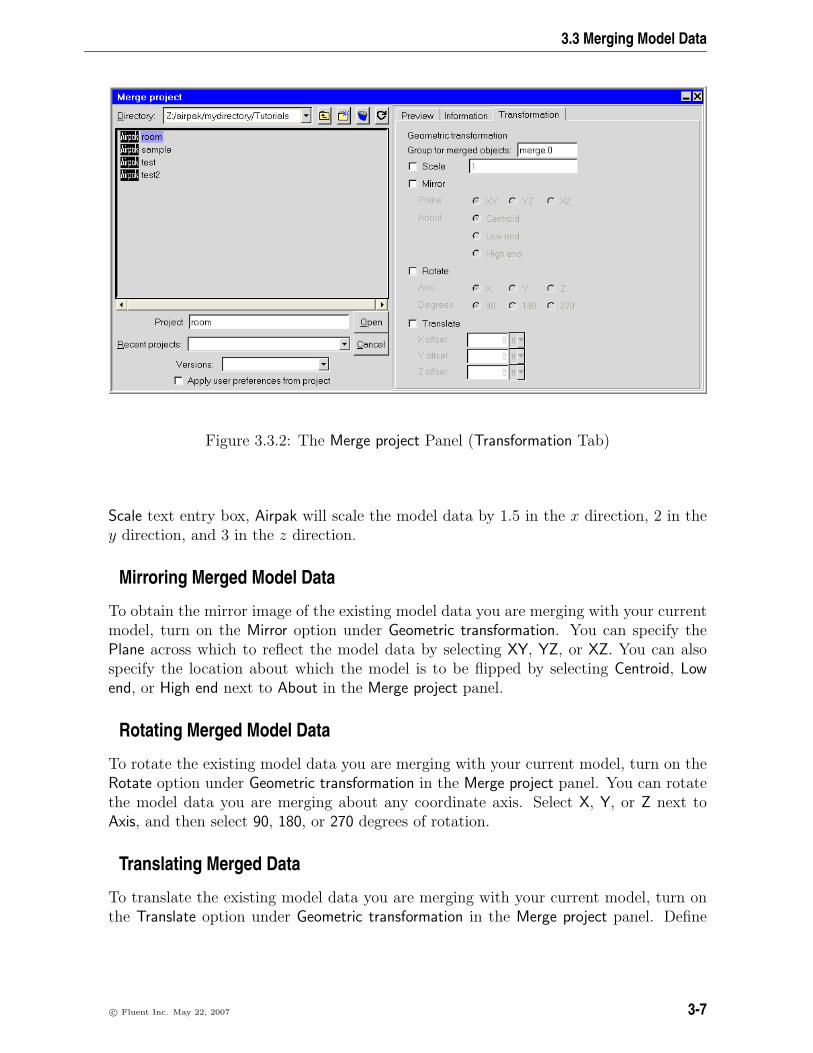
3.3 Merging Model Data
Figure 3.3.2: The Merge project Panel (Transformation Tab)
Scale text entry box, Airpak will scale the model data by 1.5 in the x direction, 2 in they direction, and 3 in the z direction.
Mirroring Merged Model Data
To obtain the mirror image of the existing model data you are merging with your currentmodel, turn on the Mirror option under Geometric transformation. You can specify thePlane across which to reflect the model data by selecting XY, YZ, or XZ. You can alsospecify the location about which the model is to be flipped by selecting Centroid, Lowend, or High end next to About in the Merge project panel.
Rotating Merged Model Data
To rotate the existing model data you are merging with your current model, turn on theRotate option under Geometric transformation in the Merge project panel. You can rotatethe model data you are merging about any coordinate axis. Select X, Y, or Z next toAxis, and then select 90, 180, or 270 degrees of rotation.
Translating Merged Data
To translate the existing model data you are merging with your current model, turn onthe Translate option under Geometric transformation in the Merge project panel. Define
c© Fluent Inc. May 22, 2007 3-7

Reading, Writing, and Managing Files
the distance of the translation from the current origin by specifying an offset in each ofthe coordinate directions: X offset, Y offset, and Z offset. Note that all offsets are relativeto the position of the existing project being merged.
3-8 c© Fluent Inc. May 22, 2007

3.4 Saving a Project File
3.4 Saving a Project File
To save the current project under its current name, click on the button in the Filecommands toolbar or select Save project in the File menu. Airpak will save the projectusing the current name.
File−→Save project
To save the current project under a different name, or for more options when saving thecurrent project, select the Save project as option in the File menu. This opens the Saveproject panel (Figure 3.4.1).
File−→Save project as
Figure 3.4.1: The Save project Panel
To save the current project, follow the steps below:
1. Specify the name of the project to be saved in the Project text entry box. Youcan choose the directory and filename in the Directory list. See Section 2.1.8 formore information on file selection. Alternatively, you can enter your own filename,which can be a full pathname to the file (beginning with a / character on a UNIXsystem or a drive letter on Windows) or a pathname relative to the directory inwhich Airpak was started. The filename can include any alphanumeric charactersand most special characters. It cannot contain control characters, spaces, tabs, orthe following characters:
$ ][ /\ " * ?
c© Fluent Inc. May 22, 2007 3-9

Reading, Writing, and Managing Files
2. Specify the Version for the project to be saved. See Section 2.1.8 for informationon versions.
3. Select any other data to be saved with the project.
• If you have created a mesh for the project, you can copy the mesh data to thenew project by selecting the Copy mesh data option.
• If you have solution data for the project, you can copy the solution data tothe new project by selecting the Copy solution data option.
• You can save postprocessing data with the project by selecting the Save post-processing objects option.
• You can save a snapshot of the model as it currently appears in the graphicswindow by selecting the Save picture file option. The picture will be displayedwhen you select the project in the Open project panel (see Section 6.2.2) orthe Merge project panel (see Section 3.3).
4. Click Save to save the current project (or click Cancel to close the panel withoutsaving the current project).
You can also use the Save project panel to delete projects (see Section 6.2.4), or to createa new directory (see Section 2.1.8).
3.4.1 Recent Projects
Airpak keeps track of the most recent projects you saved, and allows you to select onefrom the Recent projects drop-down list in the Open project panel (Figure 3.4.2). You canopen the Open project panel by choosing Existing in the New/Existing panel when startingAirpak, or at any time when you select Open project from the File menu.
3.5 Saving Image Files
Graphics window displays can be saved as image files in various formats, including TIFF,GIF, and PostScript. There may be slight differences, however, between images and theview displayed in the graphics window, since images are generated using the internalsoftware renderer, while the graphics window may utilize specialized graphics hardwarefor optimum performance.
To set image parameters and save image files, you will use the Save image panel (Fig-ure 3.5.1). To open the Save image panel, select Create image file in the File menu. Thisallows you to generate a file or a printed copy of your model as shown in the graphicswindow or in a selected region of the graphics window. Note that you can also addannotations to your image file (see Section 2.1.5).
The procedure for saving an image file is as follows:
3-10 c© Fluent Inc. May 22, 2007

3.5 Saving Image Files
Figure 3.4.2: The Open project Panel
Figure 3.5.1: The Save image Panel
c© Fluent Inc. May 22, 2007 3-11
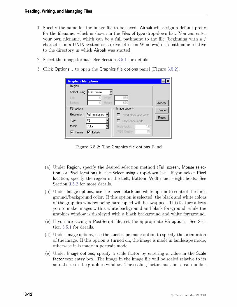
Reading, Writing, and Managing Files
1. Specify the name for the image file to be saved. Airpak will assign a default prefixfor the filename, which is shown in the Files of type drop-down list. You can enteryour own filename, which can be a full pathname to the file (beginning with a /character on a UNIX system or a drive letter on Windows) or a pathname relativeto the directory in which Airpak was started.
2. Select the image format. See Section 3.5.1 for details.
3. Click Options... to open the Graphics file options panel (Figure 3.5.2).
Figure 3.5.2: The Graphics file options Panel
(a) Under Region, specify the desired selection method (Full screen, Mouse selec-tion, or Pixel location) in the Select using drop-down list. If you select Pixellocation, specify the region in the Left, Bottom, Width and Height fields. SeeSection 3.5.2 for more details.
(b) Under Image options, use the Invert black and white option to control the fore-ground/background color. If this option is selected, the black and white colorsof the graphics window being hardcopied will be swapped. This feature allowsyou to make images with a white background and black foreground, while thegraphics window is displayed with a black background and white foreground.
(c) If you are saving a PostScript file, set the appropriate PS options. See Sec-tion 3.5.1 for details.
(d) Under Image options, use the Landscape mode option to specify the orientationof the image. If this option is turned on, the image is made in landscape mode;otherwise it is made in portrait mode.
(e) Under Image options, specify a scale factor by entering a value in the Scalefactor text entry box. The image in the image file will be scaled relative to itsactual size in the graphics window. The scaling factor must be a real number
3-12 c© Fluent Inc. May 22, 2007

3.5 Saving Image Files
greater than zero. Values greater than 1 will increase the size, while valuesless than 1 will decrease the size.
(f) Click accept to close the Graphics file options panel.
4. Click Save to save the image file (or click Cancel to close the Save image panelwithout saving the image file).
c© Fluent Inc. May 22, 2007 3-13

Reading, Writing, and Managing Files
3.5.1 Choosing the Image File Format
To choose the image file format, select one of the following items in the Files of typedrop-down list:
GIF files (*.gif) (Graphics Interchange Format) is a graphic image format.
JPEG files (*.jpg) (Joint Photographic Experts Group) is a graphic image format. Youcan define the JPEG Quality of a JPEG image under Image options in the Graphicsfile options panel (Figure 3.5.2). The maximum value of 100 will result in slightlyreduced file compression, but there will be no loss of data when the image is de-compressed. Lower values will result in more file compression, but some data willnot be recovered when the image is decompressed. The default value of 75 shouldbe acceptable for most cases.
PPM files (*.ppm) (Portable Pixmap) output is a common raster file format.
TIFF files (*.tiff) (Tagged Image File Format) is a common raster file format. TheTIFF driver may not be available on all platforms.
VRML files (*.vrml) (Virtual Reality Modeling Language) is a graphics interchangeformat that allows export of 3D geometrical entities that you can display in theAirpak graphics window. This format can commonly be used by VR systems andin particular the 3D geometry can be viewed and manipulated in a web-browsergraphics window.
i Note that non-geometric entities such as text, titles, color bars, and orienta-tion axis are not exported. In addition, most display or visibility character-istics set in Airpak, such as lighting, shading method, transparency, face andedge visibility, outer face culling, and hidden line removal, are not explicitlyexported but are controlled by the software used to view the VRML file.
Postscript files (*.ps) is a common vector file format. See below for details.
Setting Options for PostScript Files
Airpak provides several options for printing PostScript files in the Graphics file optionspanel (Figure 3.5.2). To enable the available options for making image PostScript files,select Postscript files (*.ps) from the Files of type drop-down list in the Save image panel(Figure 3.5.1) and click Options... This opens the Graphics file options panel.
3-14 c© Fluent Inc. May 22, 2007

3.5 Saving Image Files
To specify the PostScript options follow the procedure below:
1. Specify the Resolution by selecting one of the following items from the drop-downlist:
Full resolution allows you to customize the PostScript image file using the optionsin steps 2–5. Image files saved using this option will have a white backgroundinstead of the black background displayed in the graphics window.
From screen will make a PostScript image file directly from what is displayed inthe graphics window.
2. Specify the format in which the graphics window is stored in the output file byselecting PS or EPS from the Type drop-down list. EPS (Encapsulated PostScript)output is the same as PostScript output, with the addition of Adobe DocumentStructuring Conventions (v2) statements. Currently, no preview bitmap is includedin EPS output. Often, programs that import EPS files use the preview bitmap todisplay on-screen, although the actual vector PostScript information is used forprinting (on a PostScript device).
3. Specify the color mode. For a color-scale copy, select Color from the Mode drop-down list; for a gray-scale copy, select Gray; and for a black-and-white copy, selectMono. Note that most monochrome PostScript devices will render Color images inshades of gray, but to ensure that the color ramp is rendered as a linearly-increasinggray ramp, you should select Gray.
4. Enable the Frame option, if desired. If this option is turned on, a frame will beincluded around the image in the image output.
5. Enable Labels for the image, if desired. The label, which consists of the projectname, the machine name, and a date/time stamp, will appear at both the top andbottom of the page.
6. Click Accept to store the PostScript options.
3.5.2 Specifying the Print Region
There are three ways to define the region of the graphics window that should be printedto the file: you can pick the desired selection method in the Graphics file options panel,from the Select using drop-down list under Region.
Full screen instructs Airpak to use the whole graphics window as the print region.
Mouse selection allows you to select a region of the graphics window as the print region.Airpak will ask you to define the region to be written to the file. Position the mousepointer at a corner of the area to be included, hold down the left mouse button and
c© Fluent Inc. May 22, 2007 3-15

Reading, Writing, and Managing Files
drag open a selection box to the desired size, and then release the mouse button.The selected area will be printed to the file. Note that Airpak will update the Pixellocation values in the Graphics file options panel automatically when you define theregion using the mouse.
Pixel location allows you to specify a region of the graphics window as the print region.Define the bottom left corner of the print region by specifying the Left and Bottompixel locations. A value of 0 for both Left and Bottom specifies that the bottomleft corner of the print region coincides with the bottom left corner of the graphicswindow. Specify the Width and Height of the region in pixels.
This option is useful if you want to capture different images of the same size andlocation in the graphics window. First, define the region you want to capture usingthe Mouse selection option. Airpak will display the pixel location values for thisregion in the Graphics file options panel. You can then use the Pixel location optionto create further images of the same region and the same size.
3.6 Packing and Unpacking Model Files
To archive or pack up a project, select the Pack project option in the File menu.
File−→Pack project
Airpak will open the File selection dialog box (see Section 2.1.8), in which you can specifythe name of the packaged-up project. Airpak will combine all the relevant files for off-line(remote) diagnosis by your Airpak support engineer and write them to a compressed tarfile with extension .tzr. The file is in a format suitable for transfer by electronic mailor other means to your support engineer.
To unarchive or unpack a packaged-up project, select the Unpack project option in theFile menu.
File−→Unpack project
Airpak will open the File selection dialog box, in which you can specify the name ofthe packaged-up project to be unpacked. Airpak will unpack the project and displaythe model in the graphics window. (You can also unpack a project using the -unpack
command described in Section 1.5.4.)
3.7 Cleaning up the Project Data
A complete Airpak simulation can generate a significant amount of information. Youcan remove data associated with the current project from the project directory usingthe Clean up project data panel (Figure 3.7.1). You can also instruct Airpak to compressthe files associated with a particular solution ID. This option will remove any files thatare not required for further postprocessing of the solution and compress the remaining
3-16 c© Fluent Inc. May 22, 2007

3.7 Cleaning up the Project Data
files. When you postprocess the results associated with a compressed solution ID, Airpakautomatically uncompresses the files.
Figure 3.7.1: The Clean up project data Panel
The data associated with the current project are identified in the Clean up project datapanel by the operation that created them (e.g., Mesh, Post-processing), and Airpak pro-vides an estimate of the size of the data in kilobytes. The size of the total data for thecurrent project, including the data for the model itself, is given at the bottom of theClean up project data panel.
To clean up the project data, select Cleanup in the File menu.
File−→Cleanup
This opens the Clean up project data panel shown in Figure 3.7.1. The following itemsare listed in the Clean up project data panel:
Model specifies the size of the data associated with the model itself. Model datacannot be removed, since it is not possible to recreate it from other data.
Mesh specifies the size of the data resulting from the mesh generation.
Post-processing specifies the size of the data resulting from postprocessing analysis.
Screen pictures specifies the size of the data resulting from requests to store copies ofthe graphics window.
c© Fluent Inc. May 22, 2007 3-17

Reading, Writing, and Managing Files
Summary output specifies the size of the data resulting from generating a summary ofthe model objects.
Reports specifies the size of the data resulting from generating reports.
Scratch files specifies the size of any scratch files that were inadvertently left after asimulation.
Solution projectname specifies the size of the data files (i.e., .cas, .dat, .resd, etc.)resulting from running the solution. All solutions that exist for the current projectare listed by solution ID.
Version projectname specifies the size of the version files (i.e., job, model, and problem)resulting from running the solution. All versions that exist for the current projectare listed by solution ID. Version files cannot be compressed.
Total for project reports the total size of the files of all the data associated with thecurrent project, including the model data.
To delete project data, turn on the options for the data that you want to delete, andclick the Remove button at the bottom of the Clean up project data panel.
To compress project data, turn on the options for the data that you want to compress,and click the Compress button at the bottom of the Clean up project data panel.
3-18 c© Fluent Inc. May 22, 2007

Chapter 4. Importing and Exporting Model Files
You can import geometry that was created using a commercial CAD program into Airpakand also export Airpak files back into various other formats. There are several types ofCAD file formats that are supported by Airpak. This chapter describes the CAD filesthat can be imported, the way in which each type of file can be imported, and how toexport an Airpak project to other file formats.
Information in this chapter is divided into the following sections:
• Section 4.1: Files That Can Be Imported Into Airpak
• Section 4.2: Importing IGES, STEP, and Tetin Files Into Airpak
• Section 4.3: Importing Other Files Into Airpak
• Section 4.4: Exporting Airpak Files
4.1 Files That Can Be Imported Into Airpak
The following types of files can be imported into Airpak:
• International Graphics Exchange Specification (IGES) files containing point andline information (see Section 4.3)
• AutoCAD DXF files containing point and line information and DWG files containingcurves and surfaces (see Section 4.3).
• IGES and STEP (STandard for the Exchange of Product model data) files contain-ing surfaces and curves (see Section 4.2)
• Tetin files, a native ICEM-CFD file format (see Section 4.2) containing surfacesand curves.
• Comma separated values files (can be created or read in by spreadsheet programslike Excel) (see Section 4.3.5).
• Industrial Foundation Classes (IFC) 2x files (see Section 4.3)
All of these files can be imported using the File−→Import menu. Tetin and IGES/STEPfiles can also be imported using the CAD data panel (Figure 4.2.1).
The procedure for importing each type of file is described in the sections specified above.
c© Fluent Inc. May 22, 2007 4-1

Importing and Exporting Model Files
4.2 Importing IGES, STEP, and Tetin Surface Geometry Files Into Airpak
You can import IGES or STEP files that were created using a commercial CAD pack-age (e.g., Pro/ENGINEER, I-deas), or tetin files (ICEM-CFD) into Airpak for use in heattransfer and fluid flow simulations. This allows you to use a CAD engine for your geom-etry design, and transfer your model to a CAE engine for design simulation and analysis.Using a CAD/CAE partnered system allows you to quickly and accurately design, proto-type, and analyze mechanical system designs that may increase a product’s quality andsignificantly reduce its time-to-market.
Airpak provides the capability to import an IGES, STEP, or tetin file, as well as utilitiesto simplify the geometry representation and allow the geometry to be represented asAirpak objects. The following shapes can be converted into Airpak objects: rectangles,prisms, circles, cylinders, polygons, and inclined rectangular planes.
The overall Airpak process for your ventilation system design involves the following steps:
1. Model ventilation design using a CAD product.
2. Save geometry in IGES, STEP, or tetin format.
3. Import IGES, STEP, or tetin file into Airpak.
4. Convert CAD geometry into Airpak objects.
5. Conduct ventilation design analysis using Airpak.
Note that this section discusses the import of IGES or STEP files that consist of surfaces,curves, points, or a combination of the three, and tetin files that consist of surfaces andcurves. If your IGES file contains only point and line information, you can import yourfile more easily by selecting the IGES points+lines option in the File−→Import menu (seeSection 4.3).
i Importing model geometry from IGES or STEP files is not a direct way to constructa model; it is a way of creating the geometry of objects you want in your modelwithout specifying the dimensions from scratch.
4.2.1 Overview of Procedure for IGES, STEP, and Tetin File Import
The general procedure for importing an IGES, STEP, or tetin file into Airpak and cleaningup the geometry is as follows:
1. Read the IGES, STEP, or tetin file into Airpak (see Section 4.2.2).
2. Convert CAD geometry into Airpak objects (see Section 4.2.3).
4-2 c© Fluent Inc. May 22, 2007

4.2 Importing IGES, STEP, and Tetin Surface Geometry Files Into Airpak
The utilities you will use to read the IGES, STEP, or tetin file into Airpak and convertthe CAD geometry into Airpak objects are located in the CAD data panel(Figure 4.2.1)and the CAD data operation options panel (Figure 4.2.2). To open the CAD data menu,select CAD data in the Model menu.
Model−→CAD data
Click Load, and select Load IGES/Step file or Load Tetin file from the pull-down menu.
Figure 4.2.1: The CAD data Panel
Alternatively, you can import an IGES file containing surfaces and lower topology byselecting IGES/Step surfaces+curves in the File−→Import menu, or a tetin file by selectingTetin surfaces+curves in the File−→Import menu,
To open the CAD data operation options panel, select Options in the CAD data panel.
4.2.2 Reading an IGES, STEP, or Tetin File Into Airpak
When you read an IGES or STEP file into Airpak, Airpak will first convert the IGES orSTEP file into a tetin file (a native ICEM-CFD geometry format). The tetin file willthen be read into Airpak.
To read an IGES or STEP file (or tetin file) into Airpak, follow the steps below.
1. Specify a minimum feature size for imported features and specify whether you want
c© Fluent Inc. May 22, 2007 4-3

Importing and Exporting Model Files
Figure 4.2.2: The CAD data operation options Panel
Airpak to scale the room after the CAD geometry has been imported. To open theCAD data operation options panel (Figure 4.2.2), click Options in the CAD datapanel.
(a) Specify the minimum size of the features that will be imported into Airpak inthe Value text-entry field under Minimum feature size. The minimum featuresize is a global tolerance that is used by Airpak to control the level of detail thatis transferred from the IGES/STEP, or tetin file into Airpak. CAD geometrythat is smaller than the specified minimum feature size will not be read intoAirpak.
i Note that you can also remove CAD geometry that is smaller than aspecified size after you have read the IGES/STEP or tetin file into Airpak,as described in Section 4.2.4.
(b) To specify that Airpak should resize the room so that it is exactly the sizerequired to fit the CAD geometry (and any Airpak objects in your model)when it has been imported, keep the default Autoscale room option turned onin the CAD data operation options panel (Figure 4.2.2).
(c) Click Accept in the CAD data operation options panel.
2. Read the CAD geometry into Airpak. There are two ways to read an IGES, STEPor tetin file:
4-4 c© Fluent Inc. May 22, 2007

4.2 Importing IGES, STEP, and Tetin Surface Geometry Files Into Airpak
• Use the CAD data panel (Figure 4.2.1).
(a) Click Load and select one of the following options from the pull-downmenu: Load IGES/Step file or Load tetin file.
(b) Select the IGES, STEP, or tetin file in the resulting File selectiondialogbox. See Section 2.1.8 for information on the File selection dialog box.The following options are available:
– To load surface data from the IGES/STEP or tetin file, select Loadsurfaces.
– To load curve data from the IGES/STEP or tetin file, select Loadcurves.
– To load point data from the IGES/STEP or tetin file, select Loadpoints.
– (IGES or STEP import only) To copy the IGES or STEP file into thecurrent project directory, select Copy IGES file to project directory.
– (tetin import only) To load material data from the tetin file, selectLoad material. This will cause material points to be loaded from thetetin file, if any are present. These points are used to define the interiorof an object if it has been meshed with the tetrahedral mesher as aCAD object instead of being converted to an Airpak object.
– (tetin import only) To specify the triangulation tolerance, enter avalue for the Spline discretization. It is recommended that you keepthe default value. If you have a small tetin file that uses a very largeamount of memory, you can increase the Spline discretization valueslightly to fix the problem.
– To load a combination of surface, curve, and point information, selectand/or deselect the appropriate options in the File selection dialog box.
(c) Click Accept to read the IGES or tetin file into Airpak.
• Use the File−→Import menu.
File−→Import−→IGES/Step surfaces+curves,
File−→Import−→Tetin surfaces+curves,
(a) Enter the name of the IGES, STEP, or tetin file (e.g., file.igs, file.stp)in the File name field in the resulting File selection or Select tetin file panel.You can enter your own filename, which can be a full pathname to thefile (beginning with a / character on a UNIX system or a drive letter onWindows) or a pathname relative to the directory in which Airpak wasstarted. Alternatively, you can choose a filename from those availablein the Directory list. See Section 2.1.8 for more information on the Fileselection dialog box.
c© Fluent Inc. May 22, 2007 4-5

Importing and Exporting Model Files
(b) (IGES/STEP files only) To import files with a combination of surface,curve, and point data, select and/or deselect the appropriate Load surfaces,Load curves, and Load points options, respectively, in the File selectiondialog box. To copy the IGES or STEP file into the current projectdirectory, select Copy IGES file to project directory.
(c) Click Open to read the IGES, STEP, or tetin file into Airpak.
3. To read another IGES, STEP or tetin file into Airpak, repeat the steps above.
An example of an imported CAD geometry is shown in Figure 4.2.3.
Figure 4.2.3: Example of an Imported CAD Geometry
4.2.3 Using Families
A family is a group of CAD objects. Airpak will import families as part of the IGES,STEP or tetin import process if the imported file already contains them. In Airpak,
4-6 c© Fluent Inc. May 22, 2007

4.2 Importing IGES, STEP, and Tetin Surface Geometry Files Into Airpak
you can move CAD objects from one family to another, create new families, and deleteunused ones.
Airpak displays different families using different colors in the graphics window. You cantemporarily remove a family from the graphics window as described in Section 4.2.4.
Moving CAD Geometry From One Family to Another Family
To move CAD geometry from one family to another, follow the steps below.
i Note that the information below assumes that you are using the default mousecontrols in Airpak. If you have changed the default mouse controls (using the Mousebuttons section of the Preferences panel, described in Section 2.2.4), you will usedifferent mouse buttons than the ones described below to perform these operations.Airpak will inform you which mouse buttons should be used for which operationsin a message at the bottom of the graphics window.
1. Click Change family in the CAD data panel (Figure 4.2.1).
2. Select the CAD geometry in the graphics window by clicking on it using theleftmouse button or by defining a rectangular box on the screen. To define a box,position the mouse pointer at a corner of the area where the objects to be includedare located, hold down the left mouse button and drag open a selection box toenclose the objects to be included, and then release the mouse button. The objectswithin the bounded area will be selected.
To deselect the last CAD object that you selected, click the right mouse button inthe graphics window. This operation can be used repeatedly to take you back tothe first selection that you made, and then to cancel the current operation.
To deselect one particular CAD object that you have selected, hold down the<Shift> key on the keyboard and click on the object using the left mouse but-ton.
c© Fluent Inc. May 22, 2007 4-7

Importing and Exporting Model Files
The following options are also available, when appropriate, when selecting CADgeometry:
• To select all the CAD geometry in a particular family, place the mouse pointerover the graphics window and press the f key on the keyboard. Airpak willopen the Select family panel (Figure 4.2.4). Select the name of the family andclick Accept. To select all family names, click All. To deselect all selectedfamily names, click None.
Figure 4.2.4: The Select family Panel
• To instruct Airpak to select all the CAD objects that are partially inside theregion you define, place the mouse pointer over the graphics window and pressthe m key on the keyboard before you draw a box to enclose the geometry tobe selected. To instruct Airpak to select all the CAD objects that are entirelyinside the region you define, press the m key on the keyboard again before youdraw a box to enclose the geometry to be selected. By default, only CADgeometry entirely inside the region you define will be selected.
• To select all the CAD geometry within a polygon region that you define inthe graphics window, place the mouse pointer over the graphics window andpress the p key on the keyboard. The mouse pointer will change shape. Usethe left mouse button to create points in the graphics window to define thecorners of the polygon region. Click the middle mouse button when you havefinished defining the polygon region. Airpak will select all the CAD geometryenclosed in the polygon regionnder Shapes to try, select the shapes that youwant Airpak to try to fit to the CAD geometry.
i Note that restricting the shapes that you want Airpak to try to fit tothe CAD geometry will speed up the conversion process and ensure thatAirpak does not use a different type of shape than the one you require(e.g., Airpak could use a polygon shape to create a rectangle).
• Alternatively, if you want to create CAD shaped Airpak objects, you can selectthe option Use CAD surfaces directly.
• Click Options, and specify any relevant options in the CAD data operationoptions panel.
• Under Create object in the CAD data panel, click the button for the object intowhich you want to convert the CAD geometry.
4-8 c© Fluent Inc. May 22, 2007
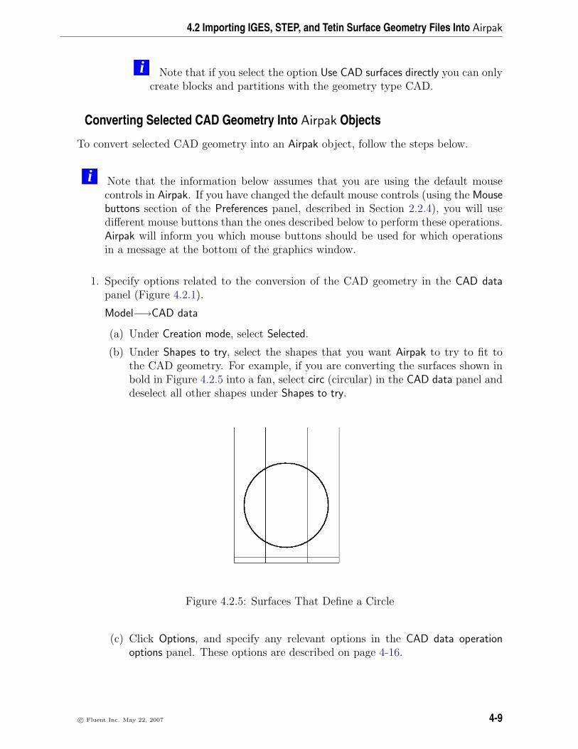
4.2 Importing IGES, STEP, and Tetin Surface Geometry Files Into Airpak
i Note that if you select the option Use CAD surfaces directly you can onlycreate blocks and partitions with the geometry type CAD.
Converting Selected CAD Geometry Into Airpak Objects
To convert selected CAD geometry into an Airpak object, follow the steps below.
i Note that the information below assumes that you are using the default mousecontrols in Airpak. If you have changed the default mouse controls (using the Mousebuttons section of the Preferences panel, described in Section 2.2.4), you will usedifferent mouse buttons than the ones described below to perform these operations.Airpak will inform you which mouse buttons should be used for which operationsin a message at the bottom of the graphics window.
1. Specify options related to the conversion of the CAD geometry in the CAD datapanel (Figure 4.2.1).
Model−→CAD data
(a) Under Creation mode, select Selected.
(b) Under Shapes to try, select the shapes that you want Airpak to try to fit tothe CAD geometry. For example, if you are converting the surfaces shown inbold in Figure 4.2.5 into a fan, select circ (circular) in the CAD data panel anddeselect all other shapes under Shapes to try.
Figure 4.2.5: Surfaces That Define a Circle
(c) Click Options, and specify any relevant options in the CAD data operationoptions panel. These options are described on page 4-16.
c© Fluent Inc. May 22, 2007 4-9

Importing and Exporting Model Files
(d) Under Create object, select the object into which you want to convert the CADgeometry.
2. Select the CAD geometry in the graphics window. See Section 4.2.3 for details onselecting and deselecting CAD geometry.
3. When you have selected all the CAD geometry to be converted to the Airpak object,click the middle mouse button in the graphics window. Airpak will convert theselected CAD geometry into an Airpak object (the type of object you selected inthe CAD data panel).
4. To convert more selected CAD geometry into Airpak objects, repeat the steps above.When you have finished converting selected CAD geometry into Airpak objects, clickthe middle mouse button in the graphics window to exit the selection mode.
Converting Families of CAD Objects Into Airpak Objects
If you select a group of families in Airpak, Airpak can convert each family in the group intoan Airpak object. For example, if the five shapes shown in bold in Figure 4.2.6 representfive different families, you can select all of these families at once and Airpak can converteach family into an Airpak object.
Figure 4.2.6: Five Families of CAD Objects
To convert families of CAD objects into Airpak objects, follow the steps below.
i Note that the information below assumes that you are using the default mousecontrols in Airpak. If you have changed the default mouse controls (using the Mousebuttons section of the Preferences panel, described in Section 2.2.4), you will use
4-10 c© Fluent Inc. May 22, 2007

4.2 Importing IGES, STEP, and Tetin Surface Geometry Files Into Airpak
different mouse buttons than the ones described below to perform these operations.Airpak will inform you which mouse buttons should be used for which operationsin a message at the bottom of the graphics window.
1. Specify options related to the conversion of the CAD geometry in the CAD datapanel (Figure 4.2.1).
Model−→CAD data
(a) Under Creation mode, select Family.
(b) Under Shapes to try, select the shapes that you want Airpak to try to fit tothe families. For example, if the five shapes shown in bold in Figure 4.2.6 areto be converted into five prism-shaped blocks, select hexa (prism) in the CADdata panel and deselect all other shapes under Shapes to try.
(c) Click Options, and specify any relevant options in the CAD data operationoptions panel. These options are described on page 4-16.
(d) Under Create object, select the object into which you want to convert the CADgeometry.
2. Select the CAD geometry in the graphics window. See Section 4.2.3 for details onselecting and deselecting CAD geometry.
3. When you have selected all the CAD geometry to be converted to Airpak objects,click the middle mouse button in the graphics window. Airpak will convert theselected CAD geometry into Airpak objects, creating one object for each familythat you selected (the type of object you selected in the CAD data panel).
4. To convert more families of CAD objects into Airpak objects, repeat the stepsabove. When you have finished converting families of CAD objects into Airpakobjects, click the middle mouse button in the graphics window to exit the selectionmode.
Converting Regions of the Model Into Airpak Objects
When converting CAD geometry into Airpak objects, you can define a region in yourmodel and then divide the region into segments. Airpak can then convert all the CADgeometry within each segment into an Airpak object. For example, you could select aCAD object that is L-shaped, as shown in Figure 4.2.7a. You could then divide the L-shaped geometry into two regions, as shown in Figure 4.2.8b. Airpak can split the CADobjects into two parts along the dividing line and then convert the CAD geometry ineach region into an Airpak object (i.e., Airpak will create two rectangular Airpak objectsfor the example shown in Figure 4.2.7.)
To convert CAD objects within a specified region into several Airpak objects, follow thesteps below.
c© Fluent Inc. May 22, 2007 4-11

Importing and Exporting Model Files
Figure 4.2.7: Converting an L-Shaped CAD Object
i Note that the information below assumes that you are using the default mousecontrols in Airpak. If you have changed the default mouse controls (using the Mousebuttons section of the Preferences panel, described in Section 2.2.4), you will usedifferent mouse buttons than the ones described below to perform these operations.Airpak will inform you which mouse buttons should be used for which operationsin a message at the bottom of the graphics window.
1. Specify options related to the conversion of the CAD geometry in the CAD datapanel (Figure 4.2.1).
Model−→CAD data
(a) Under Creation mode, select Region.
(b) Under Shapes to try, select the shapes that you want Airpak to try to fit tothe CAD geometry. For example, if you are converting the surfaces shownin Figure 4.2.7 into rectangular partitions, select quad (rectangle) in the CADdata operation options panel and deselect all other shapes under Shapes to try.
(c) Click Options, and specify any relevant options in the CAD data operationoptions panel. These options are described on page 4-16.
(d) Under Create object, select the object into which you want to convert the CADgeometry.
2. Select the CAD geometry in the graphics window. See Section 4.2.3 for details onselecting and deselecting CAD geometry.
3. When you have selected all the CAD surfaces to be converted, click the middlemouse button in the graphics window. Airpak will request that you divide up theregion you have selected into segments. Airpak will create Airpak objects for theselected CAD geometry in the regions of the model.
To divide the CAD geometry into regions, hold the mouse pointer over the place inthe graphics window where you want to create a dividing line and press the v key
4-12 c© Fluent Inc. May 22, 2007

4.2 Importing IGES, STEP, and Tetin Surface Geometry Files Into Airpak
on the keyboard to draw a vertical dividing line, or press the h key to produce ahorizontal dividing line. To create horizontal and vertical dividing lines using themouse buttons, position the pointer where you want the start of the line to be, holddown the left mouse button, drag the pointer to the desired location, and releasethe left mouse button. An example of a dividing line is shown in Figure 4.2.8 wherethe CAD geometry is divided into two regions.
To remove the last dividing line that you created, click the right mouse button inthe graphics window. This operation can be used repeatedly to take you back tothe first dividing line that you created.
Dividing line
Region 1
Region 2
Figure 4.2.8: Three CAD Objects Divided into Two Regions
4. When you have divided the CAD geometry into the appropriate regions, click themiddle mouse button in the graphics window. Airpak will open the Multiple regionspanel (Figure 4.2.9), which contains the following options:
Figure 4.2.9: The Multiple regions Panel
c© Fluent Inc. May 22, 2007 4-13

Importing and Exporting Model Files
Ignore instructs Airpak to ignore any CAD objects that are in more than oneregion and convert into Airpak objects (the type of object you selected in theModel menu) any CAD objects that are completely in the selected region. Forexample, the two square CAD objects in Figure 4.2.8 will be converted intotwo square Airpak objects and the L-shaped CAD object will be ignored.
Split instructs Airpak to split any CAD objects that are in more than one regionalong the specified dividing line and then convert the CAD geometry in eachregion into an Airpak object (the type of object you selected in the Modelmenu). For example, the L-shaped CAD object in Figure 4.2.10a will be splitalong the dividing line, and then all the CAD objects in region 1 will beconverted into one Airpak object and all the CAD objects in region 2 will beconverted into another Airpak object, as shown in Figure 4.2.10b.
Make shape instructs Airpak to convert any CAD objects that are completelyin one region into Airpak objects, and convert any CAD objects that are inmore than one region into Airpak objects. For example, the two square CADobjects in Figure 4.2.11a will be converted into two square Airpak objects, andthe L-shaped object will be converted into a large square Airpak object, asshown in Figure 4.2.11b.
Cancel instructs Airpak to exit the selection mode.
5. To convert more regions of CAD geometry into Airpak objects, repeat the stepsabove. When you have finished converting regions of CAD geometry into Airpakobjects, click the middle mouse button in the graphics window to exit the selectionmode.
4-14 c© Fluent Inc. May 22, 2007

4.2 Importing IGES, STEP, and Tetin Surface Geometry Files Into Airpak
Figure 4.2.10: Three CAD Objects Converted Into Two Airpak Objects Usingthe Split Option
Figure 4.2.11: Three CAD Objects Converted Into Three Airpak Objects Us-ing the Make shape Option
c© Fluent Inc. May 22, 2007 4-15

Importing and Exporting Model Files
CAD Import Options
The following options are available in the CAD data operation options panel (Figure 4.2.2).
Polygon options contains options for creating polygon objects from imported CADgeometry.
Max volume change allows you to specify how much the volume of a polygonor a non-uniform object can expand in order to simplify the object (e.g., byremoving polygon vertices that are almost collinear).
Max polygon points specifies the maximum number of points Airpak can use whenit creates a polygon.
Minimum feature size contains options for setting the minimum size of object featurescreated from imported CAD geometry.
Value specifies the minimum size of features to be imported into Airpak from theIGES, STEP or tetin file.
Blank below value specifies that Airpak should blank (i.e., not display) featuressmaller than the specified Minimum feature size(see above and Section 4.2.4).
Select CAD geometry types contains options for selecting which parts of the importedCAD geometry should be used to create Airpak objects.
Surfaces specifies that Airpak should use the selected surfaces to create an Airpakobject.
Curves specifies that Airpak should use the selected curves to create an Airpakobject.
Points specifies that Airpak should use the selected points to create an Airpakobject.
Materials specifies that Airpak should use the material points in a tetin file (ifpresent). These points are used to define the interior of an object if it hasbeen meshed with the tetrahedral mesher as a CAD object instead of beingconverted to an Airpak object.
Group for new objects allows you to specify the name of a group to which Airpak willadd new Airpak objects.
Allow non-uniform shapes allows Airpak to create non-uniform shapes when it tries tofind the best shape to fit to the selected CAD geometry.
Autoscale room specifies that Airpak should scale the room to be the exact size of theCAD geometry in the IGES or tetin file.
Convert bsplines to facets specifies Airpak to take the CAD surfaces that come in viatetin/step/iges import and convert to triangular facets internally, and save themin the model file. These facets are used for objects that have CAD shapes.
4-16 c© Fluent Inc. May 22, 2007

4.2 Importing IGES, STEP, and Tetin Surface Geometry Files Into Airpak
4.2.4 Visibility of CAD Geometry in the Graphics Window
There are several ways to display CAD geometry in the graphics window or remove theCAD geometry from the graphics window, either temporarily or permanently. You canalso shade any CAD geometry that is visible in the graphics window. These options aredescribed below.
Changing the Visibility of a Family of CAD Objects
To change the visibility of a family of CAD objects, open the CAD data panel (Fig-ure 4.2.1). In the Families list, click on the name of a family to select or deselect it. Afamily is selected if the region around it in the Families list is colored; it will be visiblein the graphics window. A family is deselected if the region around it in the Familieslist is not colored; it will not be visible in the graphics window. Click All to select allfamilies; click None to deselect all families. The visibility of a family will be updatedin the graphics window as soon as you select or deselect the name of the family in theFamilies list.
This option can be useful if you are working with a complicated geometry and you wantto unclutter the display. The family will be removed from the graphics window but notfrom your model.
Displaying Used and Unused CAD Geometry
Used CAD geometry is IGES or STEP geometry that has been used to create Airpakobjects; unused CAD geometry is IGES or STEP geometry that has not been used tocreate Airpak objects.
To display unused CAD geometry in the graphics window, turn on the Show unusedoption in the CAD data panel (Figure 4.2.1). To remove unused CAD geometry from thegraphics window, turn off the Show unused option.
To display used CAD geometry in the graphics window, turn on the Show used option inthe CAD data panel. To remove used CAD geometry from the graphics window, turn offthe Show used option.
The default setting in Airpak is that unused CAD geometry is displayed in the graphicswindow and used CAD geometry is removed from the graphics window.
Blanking and Unblanking CAD Surfaces
You can temporarily remove or “blank” selected CAD surfaces from the graphics window.To blank selected surfaces, follow the steps below.
i Note that the information below assumes that you are using the default mousecontrols in Airpak. If you have changed the default mouse controls (using the Mouse
c© Fluent Inc. May 22, 2007 4-17

Importing and Exporting Model Files
buttons section of the Preferences panel, described in Section 2.2.4), you will usedifferent mouse buttons than the ones described below to perform these operations.Airpak will inform you which mouse buttons should be used for which operationsin a message at the bottom of the graphics window.
Model−→CAD data
1. Click Blank in the CAD data panel (Figure 4.2.1).
2. Select the CAD surfaces to be blanked in the graphics window. See Section 4.2.3for details on selecting and deselecting CAD geometry.
3. When you have selected all the CAD geometry to be blanked, click the middle mousebutton in the graphics window. Airpak will blank the selected CAD geometry.
4. To blank more CAD geometry, repeat the steps above. When you have finishedblanking CAD geometry, click the middle mouse button in the graphics window toexit the Blank surfaces mode.
To unblank all blanked surfaces (i.e., to redisplay all CAD surfaces that you temporarilyremoved from the graphics window), click Unblank in the CAD data panel.
Model−→CAD data
You can also blank features that are smaller than a specified size in your Airpak model.To blank small features, specify the minimum size of the features that will be importedinto Airpak in the Value text-entry field under Minimum feature size in the CAD dataoperation options panel (Figure 4.2.2) and click the Blank below value button. Airpak willblank features smaller than the specified minimum feature size.
To unblank small features that you blanked using the method above, reduce the valueof the Minimum feature size in the CAD data operation options panel and click the Blankbelow value button.
i Note that you cannot use Unblank in the CAD data panel to unblank surfaces thatwere blanked using the Minimum feature size in the CAD data operation optionspanel.
Deleting All Remaining CAD Surfaces
To delete all remaining CAD surfaces from your model, click Clear in the CAD data panel(Figure 4.2.1).
Model−→CAD data
Airpak will display a warning message asking if you want to permanently remove all CADdata from your Airpak model (Figure 4.2.12). Click Yes to remove all remaining CADsurfaces.
4-18 c© Fluent Inc. May 22, 2007

4.2 Importing IGES, STEP, and Tetin Surface Geometry Files Into Airpak
Figure 4.2.12: Warning Message Before All CAD Geometry is Deleted
Shading CAD Surfaces
To shade all of the remaining CAD surfaces in the graphics window, turn on the Solidshading option in the CAD data panel (Figure 4.2.1).
Model−→CAD data
To display all of the remaining CAD surfaces in wireframe format, turn off the Solidshading option in the CAD import menu.
Manipulating CAD Geometry With the Mouse
You can modify the view of your CAD geometry in the graphics window using the mouseas described in Section 2.2.4. To enable faster movement of your model in the graphicswindow if your model is very large, turn on the Fast movement option in the CAD datapanel (Figure 4.2.1).
Model−→CAD data
Airpak will remove the curves in your model from the graphics window while youmovethe model and then redisplay the curves when you stop moving the model.
Fixing Small Gaps in the CAD Geometry
To eliminate gaps in the CAD geometry below a specified size, enter a value under Smallgaps in the CAD data panel (Figure 4.2.1) and click Fix below size.
Model−→CAD data
Airpak will merge existing curves and surfaces, create points by intersecting curves, andsplit existing surfaces as necessary to fix the specified gaps.
c© Fluent Inc. May 22, 2007 4-19

Importing and Exporting Model Files
4.3 Importing Other Files Into Airpak
This section describes how to import IGES and AutoCAD DXF files containing point andline inform, DWG and DXF Files containing surface and curve geometry, IFC files, andcomma separated values (CSV/Excel) files into Airpak.
The general procedure for importing these files is described in Section 4.3.1. Specificinformation on importing IGES and DXF files with point and line geometry is providedin Section 4.3.2 and on importing DWG and DXF files with surface geometry in Sec-tion 4.3.3.
i Importing model geometry from IGES and DXF files is not a direct way to con-struct a model; it is a way of creating the geometry of objects you want in yourmodel without specifying the dimensions from scratch.
4.3.1 General Procedure
To import model geometry into Airpak, follow the procedure below. Note that whenmodel geometry from any of the following file formats is imported into Airpak, the pointsbetween line segments are displayed in blue.
In the File−→Import menu.
File−→Import
1. Select the type of file you want to import into Airpak.
• For an IGES file that contains point and line information, select IGES points+lines.
• For a DXF file that contains point and line infomration, select DXF points+lines.
• For an DWG (or DXF) file that contains surface and curve information, selectDWG surfaces+curves.
• For a comma separated ASCII file, select CSV/Excel.
• For an IFC file, select IFC file.
2. Enter the name of the import file (e.g., file.igs) in the File name field in thedialog box. You can enter your own filename, which can be a full pathname to thefile (beginning with a / character on a UNIX system or a drive letter on Windows)or a pathname relative to the directory in which Airpak was started. Alternatively,you can choose a filename by selecting the file in the directory list in the dialogbox.
3. (IFC files only) Enter a new name for the Airpak job that you want to contain theimported data in the Job name field. If you are importing an IFC file and you leavethe Job name field blank, Airpak will assign a job name derived from the IFC filename.
4-20 c© Fluent Inc. May 22, 2007

4.3 Importing Other Files Into Airpak
4. (IGES and DXF point and line geometry files only) Keep the default option of Scaleroom to fit objects. This sizes the room automatically to the dimensions requiredto contain the imported data.
5. (DWG surface and curve geometry files only) To import a combination of surface,curve, and point data, select and/or deselect the appropriate Load surfaces, Loadcurves, and Load points options, respectively, in the File selection dialog box. Tospecify the triangulation tolerance, enter a value for the Spline discretization. It isrecommended that you keep the default value. If you have a small file that uses avery large amount of memory, you can increase the Spline discretization value slightlyto fix the problem. To load material data from the DWG file, select Load material.This will cause material points to be loaded from the file, if any are present. Thesepoints are used to define the interior of an object if it has been meshed with thetetrahedral mesher as a CAD object instead of being converted to an Airpak object.
6. Click Open to import the model data.
4.3.2 IGES and DXF Files With Point and Line Geometry
When Airpak imports geometry from an IGES or DXF file as described in Section 4.3.1,only point and line geometry are imported; all other geometric entities are ignored.In addition, the imported geometry has no physical characteristics associated with it(i.e., no thermal parameters, material properties, etc.). Consequently, when you importgeometry from these file formats into Airpak, you must assign physical characteristics toeach object.
When the model geometry is imported into Airpak, the lines that describe the importedgeometry are displayed and the ends of each line have blue dots associated with them.Any point imported from the IGES or DXF file also has a blue dot on it.
Once you have imported model data from a CAD source (see above Section 4.3.1), youcan use it in your Airpak model by following the procedure below.
First you create an object in Airpak, then you snap the Airpak object to the correspondingimported geometry. Finally you stretch the Airpak object to fit the geometry.
1. Create an object (e.g., a block) in Airpak.
2. Hold down the <Shift> key on the keyboard and use the right mouse button toselect a portion (either an edge or corner) of the Airpak object. It will becomehighlighted in red when selected.
3. Use the <Shift> key and the right mouse button to “snap” the selected portionof the Airpak object to the corresponding edge or corner of the imported geome-try. You can either drag the edge/corner of the Airpak object to the corresponding
c© Fluent Inc. May 22, 2007 4-21
Importing and Exporting Model Files
edge/corner of the imported geometry, or simply click the edge/corner of the im-ported geometry. The Message window will report that the object is snapped. TheAirpak object is now “anchored” to the imported model geometry.
4. Stretch the Airpak object until it fits the imported geometry by holdingdown the<Shift> key and using the right mouse button to drag the anchored edge or cornerto extend the length or width of the corresponding imported geometry. You onlyneed to fit two red dots to two blue dots or as few as two edges to achieve totalcoincidence in all three dimensions. The resulting object is now highlighted in theEdit panel. You can rename the object, assign it to a group, or perform any functionyou would perform on any other Airpak object, because now it is an Airpak object.
If you want to convert a number of objects from a complex imported model geometry,you can use the Visible option in the Options menu to remove the object types from themodel after you convert them in order to reduce the number of objects on the screen asyou continue to work.
Note that the CAD geometry is not saved when you save a job file; it is available onlyduring the session in which it is imported.
4-22 c© Fluent Inc. May 22, 2007

4.3 Importing Other Files Into Airpak
4.3.3 DWG and DXF Files with Surface Geometry
Airpak can import AutoCAD DWG files that contain surface information. You can thencreate Airpak objects from selected surfaces in a manner similar to that of an IGES file.See Section 4.2 for details about IGES file translation.
To import a DWG or DXF file with surfaces, curves, points, or a combination of thethree:
• In the File−→Import menu, select DWG surfaces+curves.
File−→Import−→DWG surfaces+curves
• Enter the File name in the File selection panel.
• Select Load surfaces, Load curves, Load points or a combination of the three.
• Select Load material from the DWG, ACIS or tetin file. This will cause materialpoints to be loaded from the DWG, ACIS, or tetin file, if any are present. Thesepoints are used to define the interior of an object if it has been meshed with thetetrahedral mesher as a CAD object instead of being converted to an Airpak object.
• Leave the default Spline discretization at 0.05 to specify the triangulation tolerance.If you have a small DWG, ACIS, or tetin file that uses a very large amount ofmemory, you can increase the Spline discretization value slightly to fix the problem.
• Click Open to import the file into Airpak.
4.3.4 IFC Files
Airpak can import Industrustrial Foundation Classes (IFC) 2x files that have been ex-ported from several CAD packages and other IFC write-compliant software. The Inter-national Alliance for Interoperability (IAI) has developed this language for exchangingdata used in construction and facilities management industries between software tools.IFC is an open standard supported by many commercial CAD packages.
You can import several basic types of building objects from an IFC file into Airpak directlyas Airpak objects, which significantly decreases the time required to build a model and alsoreduces the possibility of errors during geometry recreation. For example, this capabilityallows you to import architecture/engineering/construction (AEC) model data createdin other CAD programs into Airpak as walls, doors, windows, or spaces.
You can obtain information about IFC from www.iai.org.
To import an IFC file in Airpak:
• In the File−→Import menu, select IFC file.
File−→Import−→IFC file
c© Fluent Inc. May 22, 2007 4-23

Importing and Exporting Model Files
• Enter the File name in the Select IFC file panel and click Open.
See Section 4.3.1 for details.
Table 4.3.1 lists examples of IFC geometries and the corresponding Airpak objects thatwill be created upon importing the IFC file. See Chapter 7 for more information aboutspecific Airpak objects.
Table 4.3.1: Airpak Objects Created From IFC Geometry
IFC Geometry Airpak Objectdoors openings (rectangular, inclined, or polygonal)openings openings (rectangular or inclined)windows partitions (rectangular or inclined)walls partitions (rectangular, inclined, or polygonal)floorslabs partitions (prism or polygonal)spaces fluid blocks (prism or polygonal)columns hollow blocks (prism, cylindrical, or polygonal)
4-24 c© Fluent Inc. May 22, 2007

4.3 Importing Other Files Into Airpak
4.3.5 CSV/Excel Files
Airpak allows you to import geometry and power for simple objects (including blocks,walls, vents, 2D fans, resistances, openings, and sources) in the form of comma separatedvalues (CSV) files. Complex objects are not supported for this operation. Materialproperties and certain boundary conditions are also not supported for this type of import.
An example of this file format is given below. For details about how to export aCSV/Excel file, see Section 4.4.2.
# Partitions Rectangular Object
name,high_emis_on,high_reftemp,high_rtype,low_rtype,partition_type,
all_conduct_thin_thickness,fl_material,use_contact_res,eff_thick,low_enabled,
low_material,all_conduct_thin_material,all_conduct_thin_on,sol_material,
high_material,high_enabled,contact_res,te,eff_thick_on
partition.1,0,20.0,reftemp,reftemp,conduct_thin,0.0,default,0,0.01,0,default,
default,0,default,default,0,0.0,0.0,0
# Partitions Rectangular
name,xs,ys,zs,xe,ye,ze,xd,yd,zd,volume_flag,split_flag,partition_flag,diff_flag,
plane,iradius,thickness,numcopies,copyspace,xoff,yoff,zoff
partition.1,0.4,0.4,0.5,0.6,0.6,0.5,0.2,0.2,0,0,0,1,0,2,0,0,1,0,0,0,0
# Fans Circular Object
name
fan.1
# Fans Circular
name,xc,yc,zc,split_flag,plane,radius,iradius,xoff,yoff,zoff
fan.1,0.5,0.5,0.5,16,2,0.1,0,0,0,0
# Blocks Polygon Object
name
block.1
# Resistances Prism Object
name
resistance.1
# Blocks Polygon
name,volume_flag,split_flag,changes,nverts,plane,height,xoff,yoff,zoff,
vert1,tvert1,vert2,tvert2,vert3,tvert3
block.1,1,0,0,3,0,0.2,0,0,0,0.8 0 0.717157,,0.8 0.282843 0.717157,,0.8 0 1,
c© Fluent Inc. May 22, 2007 4-25

Importing and Exporting Model Files
# Resistances Prism
name,xs,ys,zs,xe,ye,ze,xd,yd,zd,volume_flag,diff_flag,xoff,yoff,zoff
resistance.1,0.8,0.241689,0.0363489,1,0.441689,0.236349,0.2,0.2,0.2,1,0,0,0,0
Typically, the flags you would use are name, xs, ys, zs, xe, ye, ze, xd, yd, zd.In many cases (e.g., for 2D objects, inclined shapes, or cylindrical shapes),plane infor-mation is also useful. This is represented by an integer value of 0, 1, or 2, where 0 mapsto yz, 1 maps to xz and 2 to xy. In general:
• xs, ys, zs represent the starting coordinates
• xe, ye, ze represent the ending coordinates
• xd, yd, zd represent the lengths in each direction.
For cylindrical or circular objects, the relevant dimensions become xc, yc, zc, radius,
height.
If you import the file from Airpak into Excel and use the comma as a separator, theneach column will get imported correctly.
To import a file from Excel into Airpak, it is recommended that you group all objecttypes and shape types together. For example, if you wish to create a number of cuboidalblocks, you might create the following input (where the commas separate columns):
# Blocks Prism
name,xs,ys,zs,xe,ye,ze,xd,yd,zd,volume_flag,diff_flag,xoff,yoff,zoff
block.1,0.4,0.4,0.4,0.6,0.6,0.6,0.2,0.2,0.2,1,0,0,0,0
block.2,0.3,0.3,0.3,0.6,0.6,0.6,0.2,0.2,0.2,1,0,0,0,0
block.3,0.4,0.4,0.4,0.6,0.6,0.6,0.2,0.2,0.2,1,0,0,0,0
Alternatively, you could input the same syntax into a text editor and then import thetext file into Airpak.
To add cylindrical blocks, for example, append the following to the previous list:
# Blocks Cylinder
name,xc,yc,zc,xc2,yc2,zc2,volume_flag,changes,plane,radius,iradius,
radius2,iradius2,height,start_angle,end_angle,xoff,yoff,zoff
block.4,0.4,0.5,0.5,0.6,0.5,0.5,1,0,0,0.112838,0,0.112838,0,0.2,0,0,0,0,0
block.5,0.4,0.5,0.5,0.6,0.5,0.5,1,0,0,0.112838,0,0.112838,0,0.2,0,0,0,0,0
block.7,0.4,0.5,0.5,0.6,0.5,0.5,1,0,0,0.112838,0,0.112838,0,0.2,0,0,0,0,0
4-26 c© Fluent Inc. May 22, 2007

4.3 Importing Other Files Into Airpak
You can proceed this way to generate as many object types and shapes as you wish.
Note that not all of the columns are necessary. It is also not necessary to create the headersection with the labels as shown above (i.e., name, xs, ys, etc.). In the following example,you will import three prism (cuboid) blocks. The starting coordinates are expressed bythe first three values and the dimensions are expressed by the last three values.
# Blocks Prism
block.1,0.4,0.4,0.4,0.2,0.2,0.2
block.2,0.3,0.3,0.3,0.2,0.2,0.2
block.3,0.4,0.4,0.4,0.2,0.2,0.2
When you import this syntax into Airpak using the CSV/Excel option in the File−→Importmenu, Airpak will ask you for inputs of units, choice of separator,and type of object bywhich to represent the input geometry. When Airpak encounters a line that begins witha #, it will pause and ask for the next set of choices. For example, if you import thefollowing syntax
# Blocks Prism
block.1,0.4,0.4,0.4,0.2,0.2,0.2
block.2,0.3,0.3,0.3,0.2,0.2,0.2
block.3,0.4,0.4,0.4,0.2,0.2,0.2
# Openings Rectangular
opening.1,0.4,0.4,0.5,0.6,0.6,0.5
opening.2,0.2,0.2,0.3,0.6,0.6,0.3
Airpak will stop after the first set of blocks and ask you how you want to import the nextset. This process will continue until Airpak reaches the end of the file.
i Note that if you do not have any lines starting with a #, your only choice will beto import all of the objects as a single type/shape.
The same procedure can be used to import power values for a set of objects.
To import power values for a set of rectangular sources you can use the followin syntax.
# Sources Rectangular Object
name,temp_total,temp_total_units
M-1,0.708813428,W
M-2,1.895909642,W
M-3,2.316375884,W
c© Fluent Inc. May 22, 2007 4-27

Importing and Exporting Model Files
i Note that for the power import, the object geometry needs to be imported/createdprior to the power values. If the object geometry is not created prior to the powerimport, the objects will be created using the default geometry.
4.4 Exporting Airpak Files
The following sections detail how to export Airpak projects in various other formats.
4.4.1 IGES, STEP, and Tetin Files
To export an IGES or STEP (or tetin) file from Airpak, select the appropriate item inthe File−→Export menu and then specify a name with the appropriate extension in theFile selection panel.
File−→Export−→IGES, File−→Export−→Step, File−→Export−→Tetin
4.4.2 CSV/Excel Files
To export an object or a list of objects in CSV/Excel file format, select the appropriateobjects in the Model manager window, and then select CSV/Excel in the File−→Exportmenu. Airpak will open the Save object panel (Figure 4.4.1), where you can specify thedetails of the object that you want to export.
File−→Export−→CSV/Excel
Figure 4.4.1: The Save object Panel for CSV/Excel Files
4-28 c© Fluent Inc. May 22, 2007

4.4 Exporting Airpak Files
After you have entered a File name, you will need to specify the type of Separator that willbe used to separate the data in the output file (i.e., tab, space, comma, or semi-colon).
If the object geometries are all that you want to export, you should turn on the Geometryonly option. However, if you also want to export other model data (e.g., radiation, heattransfer, flow direction information), leave the Geometry only option turned off and insteadclick Object output options. Airpak will then open a series of panels (e.g., Figure 4.4.2)where you can select the data to be exported.
Figure 4.4.2: An Example of a CSV/Excel Export Options Panel
In each of the export options panels, turn on the options for the data to be exportedfor the various objects. When you are done with one object, click Select in the panel toproceed to the next panel. When you are finished with all of the objects, click Save inthe Save object panel to complete the export.
i Object geometries will not be written unless General is turned on in each of theexport options panels.
c© Fluent Inc. May 22, 2007 4-29

Importing and Exporting Model Files
4-30 c© Fluent Inc. May 22, 2007

Chapter 5. Unit Systems
This chapter describes the units used in Airpak and how you can control them. Informa-tion is organized into the following sections:
• Section 5.1: Overview of Units in Airpak
• Section 5.2: Units for Meshing
• Section 5.3: Built-In Unit Systems in Airpak
• Section 5.4: Customizing Units
• Section 5.5: Units for Postprocessing
5.1 Overview of Units in Airpak
Airpak allows you to work in any unit system, including mixed units. Thus, for example,you can work in Imperial (British) units with heat input in Watts, or you can work inSI units with length defined in inches. This is accomplished by providing Airpak with acorrect set of conversion factors between the units you want to use and the standard SIunit system that is used internally. Airpak uses these conversion factors for input andoutput, internally storing all parameters and performing all calculations in SI units.
Units can be altered part-way through a problem setup and/or after you have completedyour calculation. If you have input some parameters in SI units and then you switch toImperial, all of your previous inputs (and the default prompts) are converted to the newunit system. If you have completed a simulation in SI units but you would like to reportthe results in any other units, you can alter the unit system and Airpak will convert allof the problem data to the new unit system when results are displayed. As noted above,all problem inputs and results are stored in SI units internally. This means that theparameters stored in the project files are in SI units. Airpak simply converts these valuesto your unit system at the interface level.
i Note that you must specify all inputs in SI units in the Transient temperature panel.
c© Fluent Inc. May 22, 2007 5-1

Unit Systems
5.2 Units for Meshing
The units used for meshing will be the same as the default units specified for length(meters) in Airpak. You can change the units for meshing in the Mesh Control panel.
Open the Mesh control panel (Figure 5.2.1) by selecting Generate mesh in the Model menu,
or by clicking on the button in the Model and solve toolbar.
Model−→Generate mesh
Figure 5.2.1: Portion of the Mesh control Panel (Generate Tab)
Click on the Generate tab to access the controls for mesh generation. Select the unitsyou would like to change to for a particular mesh from the drop-down list next to Meshunits (Figure 5.2.2). Click Done in the Mesh Control panel to change the meshing unitsand close the panel.
Figure 5.2.2: The Mesh units drop-down list
5-2 c© Fluent Inc. May 22, 2007

5.3 Built-In Unit Systems in Airpak
5.3 Built-In Unit Systems in Airpak
Airpak provides two built-in unit systems: Imperial and SI. You can convert all unitsfrom one system to another in the Units section of the Preferences panel.
Edit−→Preferences
Figure 5.3.1: The Units Section of the Preferences Panel
To choose the Imperial standard for all units, click on the Set all to Imperial button; toselect the International System of units (SI) standard for all units, click on the Set all toSI button. Clicking on one of these buttons will immediately change the unit system. Youcan then click Cancel to close the Preferences panel if you are not interested in customizingany units.
Changing the unit system in the Preferences panel causes all current and future inputsthat have units to be based on the newly selected unit system.
c© Fluent Inc. May 22, 2007 5-3

Unit Systems
5.4 Customizing Units
If you would like a mixed unit system, or any unit system different from the defaultSI system supplied by Airpak, you can use the Units section of the Preferences panel(Figure 5.3.1) to select an available unit or specify your own unit name and conversionfactor for each quantity.
5.4.1 Viewing Current Units
Before customizing units for one or more quantities, you may want to view the currentunits. To view the built-in definitions for a particular category, select the categoryin the Category list in the Units section of the Preferences panel (Figure 5.3.1). Thebuilt-in definitions will be displayed in the Units list. For example, to view the built-indefinitions for length, select Length in the Category list. The built-in definitions for lengthare displayed in the Units list: m, ft, cm, mm, microns, in, mil, and Cu-oz/ft2.
5.4.2 Changing the Units for a Quantity
Airpak will allow you to modify the units for individual quantities. This is useful forproblems in which you want to use one of the built-in SI unit systems, but you want tochange the units for one quantity (or for a few). If, for example, you want to use SI unitsfor your problem, but the dimensions of the geometry are given in inches, you can selectthe SI unit system and then change the unit of length from meters to inches.
Changing the Default Unit
The default unit for a particular Category is marked with an asterisk (*) in the Units list.To change the default units for a particular quantity, follow these steps:
1. Select the quantity in the Category list (they are arranged in alphabetical order) inthe Units section of the Preferences panel (Figure 5.3.1).
2. Choose a new unit from those that are available in the Units list.
3. Click Set as default under Conversion.
4. If you wish to change the units for another quantity, repeat the steps above.
5. Apply the changes to the unit system either to the current project or to this and allfuture projects. To apply changes to the unit system to the current project only,click This project in the Preferences panel. To apply changes to the unit systemto the current project and all future Airpak projects, click All projects in the Unitdefinitions panel.
5-4 c© Fluent Inc. May 22, 2007

5.4 Customizing Units
For the example cited above, you would choose Length in the Category list, and then selectin (inches) in the Units list. Airpak displays the equation for the conversion between metersand inches:
in = c ∗ (m + x0) + y0 (5.4-1)
When the Conversion factors c=39.37008, x0=0, and y0=0 are substituted into the aboveequation, it becomes
inches = 39.37008×meters (5.4-2)
You would then click Set as default to make inches the default unit of length for yourmodel (see Figure 5.3.1).
You should substitute a length in meters into Equation 5.4-2 to calculate the length ininches. For example, to convert a length of 10 m into inches:
length in inches = (39.37008× 10) inches
= 393.7008 inches
i It is not possible to edit the Conversion factors for units that are predefined in Air-pak; these units are marked as Not user-editable under Conversion (see Figure 5.3.1).
Changing the default unit for a Category in the Units section of the Preferences panelcauses all future inputs that have units in that Category to be based on the newly selecteddefault unit. For example, if you change the unit of length as described in the exampleabove, and then you create a new block, the units defined for the block that relate tolength will be in inches (see Figure 5.4.1).
Figure 5.4.1: Units Defined for Individual Inputs for a Block
Note that changing the default unit for a Category does not change the units for anyprevious inputs. Previous inputs still use the old units, so you do not need to make anychanges to them.
c© Fluent Inc. May 22, 2007 5-5
Unit Systems
Changing the Unit for an Individual Input
You can change the unit for an individual input by following the steps below:
1. Click on the unit definition to the right of the text field to display the list of availableunits.
2. Place the mouse pointer over the new list item.
3. Click the left mouse button on the item to make the new selection. The list willclose automatically and the new selection will then be displayed.
If you want to abort the selection process while the list is displayed, you can movethe pointer anywhere outside the list and click the left mouse button.
For example, if you wanted to change the unit for xE in Figure 5.4.1 from inches tometers, you would left-click on in to the right of the xE text entry field. You would thenselect m from the list of available units. The unit for xE would be changed to meters andthe units for the other parameters would remain unchanged.
The Fix values Option
You can also change the units in which a quantity is displayed, without changing its value,using the Fix values option. This option is available in the Geometry tab of the Roompanel, in the Geometry and Properties tabs of the Object panels, and in the Propertiestab of the Materials panels. The Fix values option is off by default in the Room and theObject panels.
If, for example, you specify a block of size 0.2 m × 0.2 m × 0.2 m, and then you changethe units for the dimensions of the block from meters to centimeters, the block will bedefined with dimensions of 0.2 cm × 0.2 cm × 0.2 cm. (Internally Airpak represents thisas 0.002 m × 0.002 m × 0.002 m.)
If the Fix values option is selected in the Blocks panel, and you change the units for thedimensions of the block from meters to centimeters, the values for the dimensions of theblock will change from 0.2 m to 20 cm in the Blocks panel (the internal value stays thesame, 0.2 m).
The Fix values option is on by default in the Materials panel. A database of materialsis provided with Airpak (see Section 7.7), and the units for these materials are definedas SI units by default. When the Fix values option is on in the Materials panel, you canchange the units for a quantity without changing the internal value for that quantity.For example, the default value and units for the density of air are 1 kg/m3. If you changethe units from kg/m3 to lb/ft3 for density, the value of density for air will be displayedas 0.0624 lb/ft3 in the Materials panel, and the internal value is still 1 kg/m3.
5-6 c© Fluent Inc. May 22, 2007

5.4 Customizing Units
If the Fix values option is not selected in the Materials panel and the units are changedfor a quantity, the internal value of the quantity will be changed. In the above exampleof changing the units from kg/m3 to lb/ft3 for density, the value of density for air willbe displayed as 1 lb/ft3 in the Materials panel, and the internal value will be changed to16.02 kg/m3.
5.4.3 Defining a New Unit
To create a new unit to be used for a particular quantity, follow the procedure below:
1. In the Units section of the Preferences panel (Figure 5.3.1), select the quantity inthe Category list.
2. Click the New unit button to open the New unit name panel (Figure 5.4.2).
Figure 5.4.2: The New unit name Panel
3. Enter the name of your new unit in the text entry box and click Done. The newunit will appear in the Units list in the Units section of the Preferences panel.
4. Select the new unit in the Units list, and enter the conversion factors (c, x0, andy0) under Conversion.
5. Click on Set as default under Conversion if you want the new unit to be the defaultunit for that Category.
For example, if you want to use minutes as the unit of time, select Time in the Categorylist in the Units section of the Preferences panel and click on the New button. In theresulting New unit name panel, enter min in the text entry box and click Done. The newunit min will appear in the Units list in the Units section of the Preferences panel. Enter0.016667 (which is equal to 1/60) for c under Conversion in the Unit definitions panel.
Determining the Conversion Factor, c
The conversion factor c you specify (under Conversion in the Units section of the Pref-erences panel) tells Airpak the number to multiply by to obtain your customized unit
c© Fluent Inc. May 22, 2007 5-7

Unit Systems
value from the SI unit value. Thus the conversion factor c should have the form customunits/SI units. For example, if you want the unit of length to be inches, you shouldinput a conversion factor c of 39.37008 inches/meter. If you want the unit of speed to befeet/min, you can determine the conversion factor c by using the following equation:
xft
min= y
m
s× 60 s
min× ft
0.3048 m(5.4-3)
You should input a conversion factor c of 196.85, which is equal to 60/0.3048.
5.4.4 Deleting a Unit
To delete a unit, follow the procedure below:
1. In the Units section of the Preferences panel (Figure 5.3.1), select the quantity inthe Category list.
2. Select a unit that you want to delete from the Units list.
3. Click the Delete unit button and select Accept in the Confirm panel.
5.5 Units for Postprocessing
You can choose the units for postprocessing for different variables using the Postprocessingunits panel (Figure 5.5.1). There are several ways to open the Postprocessing units panel:
• Select Postprocessing units in the Post menu.
Post−→Postprocessing units
• Select Solution monitor in the Solve menu.
Solve−→Solution monitor
This opens the Solution monitor definition panel. Next, click on the Output unitsbutton at the bottom of the Solution monitor definition panel.
• Select Define report in the Solve menu.
Solve−→Define report
This opens the Define summary report panel. Next, click on the Units button in theDefine summary report panel.
5-8 c© Fluent Inc. May 22, 2007

5.5 Units for Postprocessing
Figure 5.5.1: The Postprocessing units Panel
• Select Convergence plot in the Post menu.
Post−→Convergence plot
This opens the Solution monitor definition panel. Next, click on the Output unitsbutton at the bottom of the Solution monitor definition panel.
• Click on Summary report in the Report menu.
Report−→Summary report
This opens the Define summary report panel. Next, click on the Edit units button inthe Define summary report panel.
• Select Point report in the Report menu.
Report−→Point report
This opens the Define point report panel. Next, click on the Edit units button in theDefine point report panel.
The Postprocessing units panel shows the units defined for the different variables availablefor postprocessing. You can change the unit for a particular variable by selecting a new
c© Fluent Inc. May 22, 2007 5-9

Unit Systems
unit from the unit definition drop-down list to the right of the variable, as described inSection 5.4.2.
5-10 c© Fluent Inc. May 22, 2007

Chapter 6. Defining a Project
Once you have planned your Airpak analysis and have identified important features of theproblem you want to solve (see Section 1.4), you are ready to begin the first step in theAirpak problem solving process: defining a project. All of the functions that are neededto define a project are found in the File menu and toolbar and the Model manager window.Consequently, this chapter will begin with an overview of the File menu and its functions,followed by a discussion of the relevant portions of the Model manager window. Once youhave defined a project, you can then move on to building your model (Chapter 7).
The information in this chapter is divided into the following sections:
• Section 6.1: Overview of Interface Components
• Section 6.2: Creating, Opening, Reloading, and Deleting a Project File
• Section 6.3: Configuring a Project
• Section 6.4: Specifying the Problem Parameters
6.1 Overview of Interface Components
6.1.1 The File Menu
The File menu (Figure 6.1.1) contains options for working with Airpak projects and projectfiles. From this menu, you can open, merge, and save Airpak projects. In addition, youcan import, export, compress, and decompress files relating to your Airpak model. Thereare also utilities designed to save or print your model geometries. A brief descriptionof the File menu options is provided below. See Chapter 3 for more information aboutreading, writing, and managing Airpak project files.
New project allows you to create a new Airpak project using the New project panel.Here, you can browse through your directory structure, create a new project direc-tory, and enter a project name.
Open project allows you to open existing Airpak projects using the Open project panel.Here, you can browse through your directory structure, locate a project directory,and either enter a project name, or specify an old project name from a list of recentprojects. Additionally, you can specify a version name or number for the project.
c© Fluent Inc. May 22, 2007 6-1

Defining a Project
Figure 6.1.1: The File Menu
Merge project allows you to merge an existing project into your current project usingthe Merge project panel.
Reload main version allows you to re-open the original version of the Airpak projectwhen your project has multiple versions.
Save project saves the current Airpak project.
Save project as allows you to save the current Airpak project under a different nameusing the Save project panel.
Import provides options to import IGES, DXF, and tetin file geometries into Airpak.You also can import IFC files, as well as comma separated values or spreadsheet for-mat (CSV) using this option. See Chapter 4 for more information about importingfiles.
Export allows you to export your work as comma separated values or spreadsheetformat (CSV)or as an IGES, STEP, or tetin file. See Chapter 4 for more informationabout exporting files.
Unpack project opens a File selection dialog that allows you to browse for and decom-press .tzr files. See Section 3.6 for details.
Pack project opens a File selection dialog that allows you to compact your project intoa compressed .tzr file. See Section 3.6 for details.
6-2 c© Fluent Inc. May 22, 2007

6.1 Overview of Interface Components
Email project allows you to pack and email your project by specifying the Recipientemail address, Subject for email, and Message text. See Section 27.13 for moreinformation on emailing the project.
Cleanup allows you to clean up your project by removing or compressing data relatingto mesh, post-processing, screen captures, summary output, reports, message logs,and scratch files using the Clean up project data panel.
Print screen allows you to print a PostScript image of the Airpak model that is dis-played in the graphics window using the Print options panel. The inputs for the Printoptions panel are similar to those in the Graphics file options panel. See Section 3.5for details.
Create image file opens a Save image dialog that allows you to save your model dis-played in the graphics window to an image file. Supported file types include: GIF,JPEG, PPM, VRML, TIFF, and PS.
Shell window opens a separate window running an operating system shell. The windowis initially in the subdirectory of the Airpak projects directory that contains all thefiles for the current projects. In this window you can issue commands to theoperating system without exiting Airpak. Type exit in the window to close thewindow when you are finished using it. (Note that on Windows systems, this menuitem is called Command prompt.
Quit exits the Airpak application.
6.1.2 The File commands Toolbar
The File Commands toolbar (Figure 6.1.2) contains options for working with Airpakprojects and project files. A brief description of the File commands toolbar options isprovided below. See Chapter 3 for more information about reading, writing, and man-aging files in Airpak.
Figure 6.1.2: The File commands Toolbar
New project ( ) allows you to create a new Airpak project using the New projectpanel. Here, you can browse through your directory structure, create a new projectdirectory, and enter a project name.
c© Fluent Inc. May 22, 2007 6-3
Defining a Project
Open project ( ) allows you to open existing Airpak projects using the Open projectpanel. Here, you can browse through your directory structure, locate a projectdirectory, and either enter a project name, or specify an old project name from alist of recent projects. Additionally, you can specify a version name or number forthe project.
Save project ( ) saves the current Airpak project.
Print screen ( ) allows you to print a PostScript image of the Airpak model thatis displayed in the graphics window using the Print options panel. The inputs forthe Print options panel are similar to those in the Graphics file options panel. SeeSection 3.5 for details.
Create image file ( ) opens a Save image dialog that allows you to save your modeldisplayed in the graphics window to an image file. Supported file types include:PPM, GIF, JPEG, VRML, TIFF, and PS.
6.1.3 The Model manager Window
The Airpak Model manager window (Figure 6.1.3) provides a localized area for definingyour Airpak model and contains a project-specific listing of problem and solution param-eters.
The Model manager window is presented in a tree-like structure with expandable andcollapsible tree nodes that show or hide relevant tree items. To expand a tree node, use
the left mouse button to click on the icon on the left hand side of the tree. Tocollapse a tree node, click on the icon.
You can edit and manage your Airpak project from within the Model manager windowusing the mouse. For example, by clicking on or dragging individual items, you can editobjects, select multiple objects, edit project parameters, add groups within groups, andbreak apart assemblies. In addition, the Model manager window includes a context menu,accessible by right-clicking the mouse, that allows you to easily manipulate your Airpakmodel. See Section 2.2.2 for more information on using the mouse in the Model managerwindow.
An Airpak project is organized in the Model manager window using six different categories:
Problem setup allows you to set basic problem parameters, set the project title,and define local coordinate systems. Options include:
Basic parameters opens the Basic parameters panel where you can specifyparameters for the current Airpak model. See Section 6.4 for details.
Title/notes opens the Title/notes panel where you can enter a title andnotes for the current Airpak model.
6-4 c© Fluent Inc. May 22, 2007

6.1 Overview of Interface Components
Figure 6.1.3: An Example of the Model manager Window
c© Fluent Inc. May 22, 2007 6-5

Defining a Project
Local coords opens the Local coord systems panel where you can createlocal coordinate systems that can be used in your model other than the Airpakglobal coordinate system with an origin of (0, 0, 0). The origins of the localcoordinate systems are specified with an offset from the origin of the globalcoordinate system. See Section 7.3.7 for details.
Solution settings allows you to set Airpak solution parameters. Options include:
Basic settings opens the Basic settings panel where you can specify thenumber of iterations to be performed and convergence criteria Airpak shoulduse before starting your CFD calculations. See Section 27.7 for details.
Parallel settings opens the Parallel settings panel where you can specify thetype of parallel execution you wish to perform. Options include serial (thedefault), parallel, or network parallel. See Section 27.11.3 for details.
Advanced settings opens the Advanced solver setup panel where you canspecify the discretization scheme, under-relaxation factors, and the multigridscheme. See Chapter 27 for details.
Libraries lists the libraries used in your Airpak project. By default, a Main libraryexists in your Airpak project that contains materials (fluids, solids, and surfaces),fan objects, and packages. See Section 7.7 for details.
Groups lists any groups of objects in the current Airpak project. See Section 7.6for details about grouping objects.
Post-processing lists any postprocessing objects in the current Airpak project.See Chapter 28 for details about postprocessing in Airpak.
Points lists any point monitoring objects in the current Airpak project. SeeSection 27.8.1 for details about point monitors.
Trash lists any objects that have been deleted from the Airpak model.
Inactive lists any objects that have been made inactive in the Airpak model.
Model lists all active objects and materials for the Airpak project.
6-6 c© Fluent Inc. May 22, 2007

6.2 Creating, Opening, Reloading, and Deleting a Project File
6.2 Creating, Opening, Reloading, and Deleting a Project File
6.2.1 Creating a New Project
The first step in the process of defining a project is to create a new project file. To do
this, select New project in the File menu or click on the button in the File commandstoolbar.
File−→New project
Airpak will open the New project file selection dialog box (Figure 6.2.1). Here, you canselect a project name, choose a location for the project, then click Create to create thenew project. For more information on file selection dialog boxes, see Section 2.1.8.
Figure 6.2.1: The New project File Selection Dialog Box
The Message window will report
Creating new project
Done loading.
In addition, a new directory for your project (e.g., project2) will be created, and thedefault room will be displayed in the graphics window.
If you are creating a new project and already have a project open that has not beenwritten to a file, Airpak will display a warning message as shown in Figure 6.2.2.
To save the current project before opening the new project, click the Save button. Air-pak will open the Save project panel, where you can specify the name of the file. (SeeSection 3.4 for more details on saving a project file.) To start the new project withoutsaving the current project, click the Don’t save button. Alternatively, to cancel openingthe new project, click the Cancel switch button.
c© Fluent Inc. May 22, 2007 6-7

Defining a Project
Figure 6.2.2: Warning Message Displayed When Opening a New Project Be-fore Saving the Current Project
Title and Notes
You can enter a title and some notes for your new Airpak project in the Title/notes panel(Figure 6.2.3). To open the Title/notes panel, double-click on the Title/notes item underthe Problem setup node in the Model manager window.
Problem setup−→ Title/notes
To enter a title and notes for your project:
1. Enter a title in the Title text entry box. The title can be longer and more descrip-tive than the project name. The title can be displayed in the graphics windowby toggling Project title in the Display drop-down list in the View menu (see Sec-tion 2.1.2).
2. Enter notes for the project in the Notes text entry box. There is no restrictionon the number and type of text characters you can use in your project’s title andnotes.
3. Click Accept.
6.2.2 Opening an Existing Project
You will use the Open project panel (Figure 6.2.4) to open an existing project. To do this,
select Open project in the File menu or click on the button in the File commandstoolbar.
File−→Open project
6-8 c© Fluent Inc. May 22, 2007
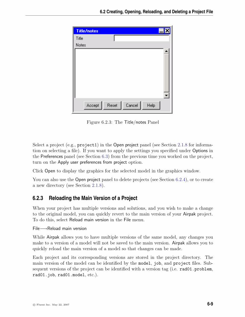
6.2 Creating, Opening, Reloading, and Deleting a Project File
Figure 6.2.3: The Title/notes Panel
Select a project (e.g., project1) in the Open project panel (see Section 2.1.8 for informa-tion on selecting a file). If you want to apply the settings you specified under Options inthe Preferences panel (see Section 6.3) from the previous time you worked on the project,turn on the Apply user preferences from project option.
Click Open to display the graphics for the selected model in the graphics window.
You can also use the Open project panel to delete projects (see Section 6.2.4), or to createa new directory (see Section 2.1.8).
6.2.3 Reloading the Main Version of a Project
When your project has multiple versions and solutions, and you wish to make a changeto the original model, you can quickly revert to the main version of your Airpak project.To do this, select Reload main version in the File menu.
File−→Reload main version
While Airpak allows you to have multiple versions of the same model, any changes youmake to a version of a model will not be saved to the main version. Airpak allows you toquickly reload the main version of a model so that changes can be made.
Each project and its corresponding versions are stored in the project directory. Themain version of the model can be identified by the model, job, and project files. Sub-sequent versions of the project can be identified with a version tag (i.e. rad01.problem,rad01.job, rad01.model, etc.).
c© Fluent Inc. May 22, 2007 6-9

Defining a Project
Figure 6.2.4: The Open project Panel
6.2.4 Deleting a Project
You can use the Open project panel (Figure 6.2.4) to delete an existing project. To do
this, select Open project in the File menu or click on the button in the File commandstoolbar.
File−→Open project
To delete an existing project, select the project (e.g., project1) in the Open project panel
(Figure 6.2.4) and then click on the button. When you delete a project, the projectsub-directory (e.g., /project1) and all the files in it that were created for the projectare deleted. A dialog box will ask you to confirm the deletion.
You can also delete projects in the Merge project panel (see Section 3.3) and the Saveproject panel (see Section 3.4).
6-10 c© Fluent Inc. May 22, 2007

6.3 Configuring a Project
6.3 Configuring a Project
You can configure your graphical user interface for the current project you are running,or for all Airpak projects, using the Options node of the Preferences panel (Figure 6.3.1).
Edit−→Preferences
Figure 6.3.1: The Preferences Panel
When you click on one of the item nodes under the Options node, the Preferences panel(Figures 6.3.2–6.3.5) will change to allow you to define many configuration settings foryour Airpak project.
c© Fluent Inc. May 22, 2007 6-11

Defining a Project
The settings that are specified when any of the items under Options are selected in thePreferences panel are stored in a file named .airpak config, which is located in yourhome directory. You should not modify the .airpak config file directly; instead, makeyour desired configuration changes in the Preferences panel. The settings specified underDefaults apply directly to the Airpak model, and are not related to how the model isdisplayed or how you interact with the model. These are saved in .airpak defaults.
The default settings for the Preferences panel are appropriate for many applications. Toreset the panel to the default settings, click the Reset all button at the bottom of thepanel (Figure 6.3.1). You can make changes to the Preferences panel, and apply thechanges either to the current project by clicking This project, or to all Airpak projectsby clicking on the All projects button. To close the panel without applying any changes,click Cancel.
A description of each item under the Options node in the Preferences panel is providedbelow. For other items in this panel, please see the appropriate section.
i If you want to load project-specific Options that were saved during a previous Airpaksession, you will need to turn on the Apply user preferences from project option inthe Open project panel the next time you load the project. See Section 6.2.2 formore information about opening a project.
6.3.1 Display Options
To set display options for your model, select the Display item under the Options node inthe Preferences panel.
Options−→ Display
Color legend data format specifies the format of the labels that define the color divi-sions in the color legend for a postprocessing object (see Section 28.2.2 for detailsabout the color legend and spectrum). The following data formats are available inAirpak:
exponential displays real values with a mantissa and exponent (e.g., 1.0e-02).You can define the number of digits in the fractional part of the mantissa inthe Color legend precision field.
float displays real values with an integral and fractional part (e.g., 1.0000). Youcan set the number of digits in the fractional part by changing the value ofthe Color legend precision.
general displays real values with either float or exponential form, depending onthe size of the number and the defined Numerical display precision.
6-12 c© Fluent Inc. May 22, 2007

6.3 Configuring a Project
Figure 6.3.2: The Display Section of the Preferences Panel
c© Fluent Inc. May 22, 2007 6-13

Defining a Project
Numerical display precision defines the number of fractional digits displayed in the la-bels for the color legend.
Color objects gray contains options for changing the color of objects in the graphicswindow to gray.
None specifies that no objects are to be colored gray.
Unselected assemblies specifies that only assemblies that are not selected shouldbe colored gray.
All specifies that all objects are to be colored gray.
Display object names contains options for displaying the names of Airpak objects in thegraphics window. You can select from the following options, or you can click the
button in the Viewing options toolbar to cycle through them.
None specifies that no object names are displayed.
Selected object specifies that only the name of the selected object is displayed.
Current assembly specifies that the names of all objects in the current assemblyare displayed. If no assemblies are defined, the names of all objects under theModel node are displayed.
Screen up direction allows you to choose the direction of the vertical axis to be eitherY or Z.
Display scale allows you to specify the scaling for the display of your project in thegraphics window. For example, if you have a long and thin model (x=10 m,y=0.1 m, z=0.1 m), you may want to view the model so that all directions areon the same scale in the graphics window. For the above example, you would enter0.01 for X, 1 for Y, and 1 for Z.
Background color allows you to specify the background color of the graphics windowby opening a Select the new background color window (or a similar panel, dependingon the platform of your machine). Since this window is not a part of the Airpakapplication, the procedure for changing the color will vary by platform.
6.3.2 Editing Options
To set editing options for your model, select the Editing item under the Options node inthe Preferences panel.
Options−→ Editing
Default dimensions allows you to specify whether you want Start/end or Start/lengthas the default selection for dimensions in the Room panel, the Object panels, andsome of the Macros panels.
6-14 c© Fluent Inc. May 22, 2007

6.3 Configuring a Project
Figure 6.3.3: The Editing Section of the Preferences Panel
Annotation edit key specifies which keyboard key is used in conjunction with the mousebuttons to move legends, titles, etc. in the graphics window. You can select Control(for the <Control> key), Shift (for the <Shift> key), or Meta (for the <Alt> key).
i Note that, in this manual, descriptions of operations that use the Annotationedit key assume that you are using the default setting (i.e., Control). If youchange the default setting, you will need to use the key you have specified, in-stead of the <Control> key, when you move legends, titles, etc. in the graphicswindow.
Fix values contains options for fixing the values of quantities in the various objectpanels. See Chapter 5 for details.
All specifies that the values of all quantities will be fixed. This will cause theFix values option to be unavailable in the Object and Room panels.
None specifies that no quantities will be fixed. This will also cause the Fix valuesoption to be unavailable in the Object and Room panels.
Per-object specifies that the Fix values option can be toggled on or off for eachindividual object. This is the default selection.
6.3.3 Printing Options
To set printing options for your model, select the Printing item under the Options nodein the Preferences panel.
Options−→ Printing
Print command for text files (UNIX systems only) designates the command used toprint text files. The symbols %p and %f designate the printer name and filename,respectively. When the command is issued, Airpak replaces %p with the name ofyour default printer (specified by the LPDEST environment variable). You can also
c© Fluent Inc. May 22, 2007 6-15

Defining a Project
Figure 6.3.4: The Printing Section of the Preferences Panel
specify the printer name explicitly (e.g., -dmyprinter). Airpak will replace %f withthe name you specify for the file. The default command is
lp -d%p %f
The symbol %t can be used to denote a temporary file whose name is uniquelygenerated by Airpak.
This command is not used by Windows systems. The Windows Print menu can beused instead.
Print command for PS files (UNIX systems only) is the command used to print PostScript(PS) files. The default command is the same as the Print command for text files,described above.
This command is not used by Windows systems. The Windows Print menu can beused instead.
6-16 c© Fluent Inc. May 22, 2007

6.3 Configuring a Project
6.3.4 Miscellaneous Options
To set other miscellaneous options for your model, select the Misc item under the Optionsnode in the Preferences panel.
Options−→ Misc
Figure 6.3.5: The Misc Section of the Preferences Panel
Xterm options (UNIX systems only) allows you to specify options for the text windowthat is opened using the Shell window item in the File menu. See Section 2.1.2 formore details on opening a text window.
Bubble help delay allows you to specify the delay time before the bubble help appearswhen you hold your mouse pointer over an item in the GUI. To disable the bubblehelp, specify a Bubble help delay of 0.
6.3.5 Editing the Library Paths
The Libraries section of the Preferences panel (Figure 6.3.6) allows you to change the pathsettings to include libraries of macros and materials so that Airpak can find them.
Options−→ Libraries
The path to the default Airpak library is displayed in the Location text field. By default,this library contains information about the materials (see Section 7.7) and macros (seeChapter 25) that are predefined in Airpak.
If you have materials or macros that are not predefined in Airpak, but you want to includethem in your model, you can add new libraries to the list. When you start Airpak, itwill load the material and macro information from the libraries specified in the list. SeeSection 7.7.6 for information about creating a user-defined materials file.
The following operations can be performed in the Libraries section of the Preferencespanel:
• To create a new library, click New library. Enter a name for the library in the Libraryname text field and then enter the path in the Location text field or click Browse tosearch for a specific directory.
c© Fluent Inc. May 22, 2007 6-17

Defining a Project
Figure 6.3.6: The Libraries Section of the Preferences Panel
6-18 c© Fluent Inc. May 22, 2007

6.3 Configuring a Project
• To modify an existing library path, select the library in the list of libraries andthen edit the path in the Location text field, or click Browse to search for a specificdirectory.
• To delete a library, select the library name in the list of libraries and click Deletelibrary.
You can make changes to the Libraries section of the Preferences panel, and apply thechanges either to the current project by clicking This project, or to all Airpak projectsby clicking All projects. Click Cancel to close the Preferences panel without saving thechanges. Once you have created a new library, a new node appears under the Librariesnode in the Model manager window.
Changing the Name of a Library
To change the name of any user-defined library, right-click on the specified library nodeand select Edit info in the resulting pull-down menu. Airpak will open the Library nameand info panel (Figure 6.3.7), where you can change the Name or add any descriptiveinformation in the large text entry field.
Figure 6.3.7: The Library name and info Panel
Adding Items to a Library
To add an item to a new library, select the item in the Model manager window and dragthe item into the new library node. If the item you drag into the library is a material,a Materials node will appear under the new library node containing the new material
c© Fluent Inc. May 22, 2007 6-19

Defining a Project
item in its appropriate category (Solid, Fluid, Surface, etc.). If the item you drag into thelibrary is an object or assembly, Airpak will open a Save project panel. You will need tosave the object or assembly as a separate project to make it available in the new library.See Section 3.4 for details about using the Save project panel.
6.3.6 Editing the Graphical Styles
The Object types section of the Preferences panel (Figure 6.3.9) allows you to customizethe color, line width, shading, decoration, and font type of individual objects associatedwith your Airpak model, as they are displayed in the graphics window. For example,you may want to change the shading of a rack of PCBs to a different type to betterdistinguish it from other objects in your graphics window. The types of objects that youcan customize in the Graphical styles panel are listed in Table 6.3.1. A description of eachoption in the Object types section of the Preferences panel follows.
Options−→ Object types
Figure 6.3.8: The Object types Section of the Preferences Panel
Color displays the color currently associated with the corresponding object type. Whenyou click on this option, a color palette menu opens. You can replace the defaultcolor for an object by selecting the new color in the color palette menu. To selecta different color, click on the icon in the lower right corner of the palette menu.Select a new color using the method or panel that is appropriate to your system.
6-20 c© Fluent Inc. May 22, 2007

6.3 Configuring a Project
Table 6.3.1: Object Choices for Editing Graphical Styles
Object DescriptionRoom Airpak roomPersons Hoods Airpak modeling objectsBlocks FansOpenings WallsPartitions SourcesResistances VentsWires AssembliesHeat exchangersCad point Reference points and lines associated withCad line model geometry that have been imported
from IGES or DXF files.Highlight The color to which a model object changes
when it is selected or becomes highlighted.Assemblies Any object, including a group, that you
have created for reuse, and is storedeither internally in the model or in aseparate user-defined location.
Meshed sep. Any assembly that is meshed separatelyassemblies from the rest of the model.Title The title and date of the model that canDate be displayed in the graphics window.Names The names of model objects that can be
optionally displayed with the object.Mesh hexa The elements that comprise the mesh forMesh penta volumes and surfaces.Mesh quadMesh barMesh qualityMesh selectedMesh adjacent
c© Fluent Inc. May 22, 2007 6-21
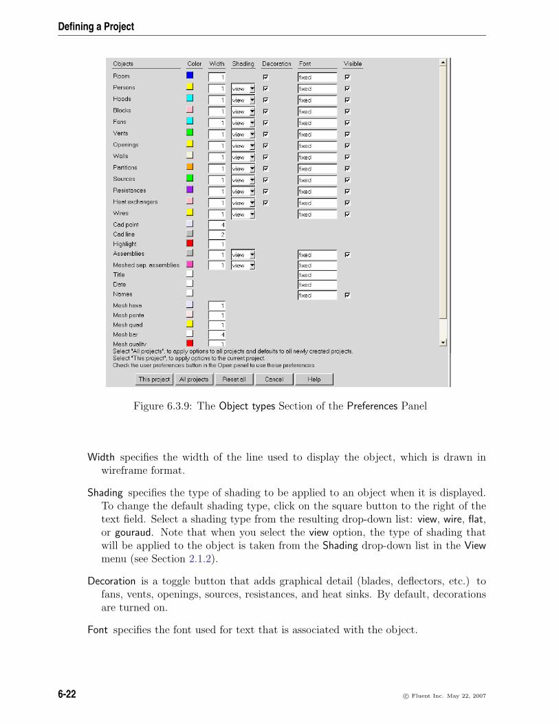
Defining a Project
Figure 6.3.9: The Object types Section of the Preferences Panel
Width specifies the width of the line used to display the object, which is drawn inwireframe format.
Shading specifies the type of shading to be applied to an object when it is displayed.To change the default shading type, click on the square button to the right of thetext field. Select a shading type from the resulting drop-down list: view, wire, flat,or gouraud. Note that when you select the view option, the type of shading thatwill be applied to the object is taken from the Shading drop-down list in the Viewmenu (see Section 2.1.2).
Decoration is a toggle button that adds graphical detail (blades, deflectors, etc.) tofans, vents, openings, sources, resistances, and heat sinks. By default, decorationsare turned on.
Font specifies the font used for text that is associated with the object.
6-22 c© Fluent Inc. May 22, 2007

6.3 Configuring a Project
Visible toggles whether the specified type of object will be visible in the graphicswindow.
6.3.7 Interactive Editing
The Interaction section of the Preferences panel (Figure 6.3.10) allows you to performsnapping when repositioning an object in the graphics window. Snapping can be doneby:
• using a grid-snap technique to position the room or an object at specified discretedistances along each axis.
• using an object-snap technique to position an object using a vertex, line, or planeof another object.
Options−→ Interaction
Figure 6.3.10: The Interaction Section of the Preferences Panel
You can set the global size of the grid independently along each axis. To set the globalsize of the grid for this project only, follow the steps below.
1. Select X grid, Y grid, and/or Z grid in the Interaction section of the Preferences panel.
2. Enter values for X grid, Y grid, and/or Z grid in the relevant text entry fields.
3. Click This project.
c© Fluent Inc. May 22, 2007 6-23

Defining a Project
You can set the object snap length by specifying a value (in pixels) for the Snap Tolerance.When this value has been set, and the model is oriented in one of the X, Y, or Z views,a dragged object will automatically snap into alignment with a second object of similarshape when it comes within the specified number of pixels of a vertex, line, or plane ofthe second object.
See Section 7.3.7 for more information about moving objects and setting object interac-tion parameters.
To set the global size of the grid or the object snap length for all Airpak projects, followthe procedure above, but click All projects (instead of This project) in the Interactionsection of the Preferences panel (Figure 6.3.10). Airpak sets the values for the grid-snapdistances to 1 and the object snap length to 10 by default, and uses the default lengthunits for your model. If none of the snap options are selected, the movement of the roomor the object using the mouse will be continuous.
6.3.8 Meshing Options
To set meshing options for your model, select the Meshing item under the Defaults nodein the Preferences panel (Figure 6.3.11).
Defaults−→ Meshing
Figure 6.3.11: The Meshing Section of the Preferences Panel
Mesh type is used to specify the type of mesh to be used in your Airpak project. Bydefault, Airpak uses the Hexa unstructured option which denotes an unstructuredhexahedral mesh. The other mesh types you can choose from are Hexa cartesianand Tetra (i.e. tetrahedral).
Minimum object separation is used to specify the minimum distance separating objectsin your model in the x, y, and z coordinate directions. This distance may beexpressed in any valid number format (e.g., 0.001, 1e-3, 0.1e-2). This specificationis used by Airpak whenever the distance between two objects is less than this value,but greater than the model’s zero tolerance.
6-24 c© Fluent Inc. May 22, 2007
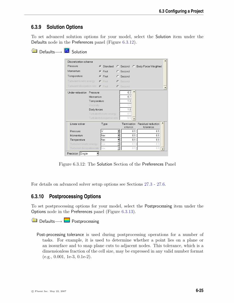
6.3 Configuring a Project
6.3.9 Solution Options
To set advanced solution options for your model, select the Solution item under theDefaults node in the Preferences panel (Figure 6.3.12).
Defaults−→ Solution
Figure 6.3.12: The Solution Section of the Preferences Panel
For details on advanced solver setup options see Sections 27.3 - 27.6.
6.3.10 Postprocessing Options
To set postprocessing options for your model, select the Postprocessing item under theOptions node in the Preferences panel (Figure 6.3.13).
Defaults−→ Postprocessing
Post-processing tolerance is used during postprocessing operations for a number oftasks. For example, it is used to determine whether a point lies on a plane oran isosurface and to snap plane cuts to adjacent nodes. This tolerance, which is adimensionless fraction of the cell size, may be expressed in any valid number format(e.g., 0.001, 1e-3, 0.1e-2).
c© Fluent Inc. May 22, 2007 6-25

Defining a Project
Figure 6.3.13: The Postprocessing Section of the Preferences Panel
Surface probe color allows you to change the color of the probed point and text. Tochange the color, click the colored rectangular next to Surface probe color. This willopen a color palette menu. To select a different color, click on the icon in the lowerright corner of the palette menu.
6.3.11 Other Preferences and Settings
When you click on other items in the Preferences panel, you will be able to edit additionalpreferences as follows:
Units allows you modify the default unit definitions and conversion factors. SeeChapter 5 for details.
Mouse buttons allows you to change the default mouse controls in Airpak. SeeSection 2.2.4 for details.
Error reporting allows you to pre-fill the Error report panel with the followinginformation necessary to email a report: Your name, Your email address, HTTPproxy host (if any), and HTTP proxy port, as shown in Figure 6.3.14.
Figure 6.3.14: The Error reporting Section of the Preferences Panel
6.4 Specifying the Problem Parameters
You can specify parameters for the current model in Airpak using the Basic parameterspanel (Figures 6.4.1, 6.4.2, 6.4.3, and 6.4.4). The types of parameters you can use todescribe your model include the following:
6-26 c© Fluent Inc. May 22, 2007

6.4 Specifying the Problem Parameters
• time variation
• solution variables
• species transport
• IAQ/comfort
• flow regime
• gravity
• ambient values
• default fluid, solid, and surface materials
• initial conditions
The default settings for the Basic parameters panel are as follows:
• steady-state
• solution of flow (velocity and pressure), temperature, and surface-to-surface radia-tion solution variables
• no species transport
• IAQ/thermal comfort postprocessing calculations activated
• turbulent flow
• natural convection included, compass setting with north in x direction
• ambient temperature of 20C, ambient pressure of 0 N/m2, ambient radiation tem-perature of 20C
• fluid is air, solid is brick, and surface is non-metallic paint.
• ambient temperature and no flow for initial conditions
To open the Basic parameters panel (Figures 6.4.1, 6.4.2, 6.4.3, and 6.4.4), double-click onthe Basic parameters item under the Problem setup node in the Model manager window.
Problem setup−→ Basic parameters
There are four push buttons at the bottom of the Basic parameters panel. To accept anychanges you have made to the panel and then close the panel, click Accept. To undoall the changes you have made in the panel and restore all items in the panel to theiroriginal states when the panel was opened, click on the Reset button. To close the paneland ignore any changes made to it, click Cancel. To access the on-line documentation,click Help.
c© Fluent Inc. May 22, 2007 6-27

Defining a Project
Figure 6.4.1: The Basic parameters Panel (General setup Tab)
Figure 6.4.2: The Basic parameters Panel (Transient setup Tab)
6-28 c© Fluent Inc. May 22, 2007
6.4 Specifying the Problem Parameters
6.4.1 Time Variation
Airpak allows you to solve two types of flow problems:
• steady-state
• transient
The default setting for time variation in the Basic parameters panel (Transient setup tab) issteady-state (Figure 6.4.2). The procedure for defining a transient simulation is describedin Chapter 20.
6.4.2 Solution Variables
Airpak allows you to choose the variables you want it to solve in your simulation. Fouroptions are presented in the Basic parameters panel (General setup tab): Flow (veloc-ity/pressure), Temperature, Radiation, and Species. (Figure 6.4.1). These options arediscussed below.
Flow, Temperature, and Species Variables
Airpak allows you to solve the problem for any of the following combinations of flow,temperature, and/or species variables:
• flow (velocity and pressure fields) only
• flow and temperature distributions (velocity, pressure, and temperature fields)
• temperature distribution only
• species transport
In the case of temperature distribution only, the flow solution from a previous simulation(for the same problem with an identical mesh) can be used to supply a velocity field forthe thermal simulation. This is useful when the dominant mechanism for heat transferby the fluid is forced convection, rather than natural convection (see Section 6.4.4 formore details on forced and natural convection). In this case, the solution of the energyequation does not affect the flow solution, so these systems can be solved independentlyrather than as a coupled simulation. The flow-only simulation can be performed first,followed by multiple thermal simulations, if required.
i You must include either flow variables or temperature variables in your simulation,or both.
c© Fluent Inc. May 22, 2007 6-29

Defining a Project
To select the variables to be solved, follow one of the procedures below:
• To solve the problem for flow, select Flow (velocity/pressure) under Variables solvedin the General setup tab of the Basic parameters panel (Figure 6.4.1). You must alsospecify the Flow regime in the General setup tab of the Basic parameters panel to beLaminar or Turbulent (see Section 6.4.3 for more details on selecting a flow type).
• To solve the energy equation for the temperature distribution together with theflow equations, select both Flow (velocity/pressure) and Temperature under Variablessolved in the General setup tab of the Basic parameters panel.
• You can also solve first for the flow, and then for the temperature. This approachis valid only if the solution of the energy equation does not affect the flow solution,which is the case if forced convection is the dominant heat transfer mechanism andthe Gravity vector is not enabled in the Basic parameters panel (General setup tab). Tosolve only for temperature using a previous solution, specify the ID for the previoussolution next to Restart in the Solve panel and select Full data under Restart. Toopen the Solve panel, select Run solution in the Solve menu. See Section 27.11.1 fordetails on restarting a calculation using a previous solution. The previous solutionwill be used to access the flow field for use in solving the energy equation. Note thatsolving only for temperature using a velocity field of zero is equivalent to solvingonly for heat conduction.
• To solve the problem for species, select On for Species in the General setup tabof the Basic parameters panel (Figure 6.4.1). The procedure for defining a speciestransport calculation is descripted in Chapter 21.
Airpak also includes the capability to predict indoor air quality (IAQ) parameters, suchas the mean age of air, and thermal comfort parameters including the mean radianttemperature, predicted mean vote (PMV), and predicted percentage dissatisfied (PPD).By default, Airpak performs a supplementary calculation immediately after the solutionof the flow, temperature, and species equations to compute the mean age of air and themean radiant temperature. If you do not want to calculate the mean age of air and themean radiant temperature for your simulation, select Off next to IAQ/Comfort in theProblem setup panel. See Section 30.2.8 for details on calculating PMV and PPD.
Radiation Variables
You can choose whether to solve the problem for radiation. If you want to solve forradiation, select On for Radiation in the General setup tab of the Basic parameters panel(Figure 6.4.1). If you do not want to solve for radiation, select Off. The surface-to-surfaceradiation model is used for modeling radiation by default. If you want to use the discreteordinates (DO) radiation model instead, select the Discrete ordinates radiation model inthe Basic parameters panel.
See Chapter 22 for information on radiation modeling.
6-30 c© Fluent Inc. May 22, 2007

6.4 Specifying the Problem Parameters
Postprocessing for Solution Variables
Airpak provides postprocessing options for displaying, plotting, and reporting the solutionvariables. The following variables are contained in the Variable and Value drop-downlists that appear in the postprocessing and reporting panels. See Chapter 30 for theirdefinitions.
Velocity-related quantities that can be reported are as follows:
• UX
• UY
• UZ
• Speed
• Velocity
• Mass flow
• Volume flow
• Angular deviation
Pressure-related quantities that can be reported are as follows:
• Pressure
Temperature-related quantities that can be reported are as follows:
• Temperature
• Heat flux
• Heat flow
• Heat tr. coeff
Species-related quantities that can be reported are as follows:
• species (mass), the mass fraction of a species
• species (mole), the mole fraction of a species
c© Fluent Inc. May 22, 2007 6-31

Defining a Project
IAQ/comfort-related quantities that can be reported are as follows:
• Relative humidity
• Mean age of air
• Radiation temp, the mean radiant temperature
• PPD
• PMV
Radiation-related quantities that can be reported are as follows:
• Radiative heat flow
6.4.3 Flow Regime
Turbulent flows are characterized by fluctuating velocity fields. These fluctuations mixtransported quantities such as momentum and energy, and cause the transported quanti-ties to fluctuate as well. Since these fluctuations can be of small scale and high frequency,they are too computationally expensive to simulate directly in practical engineering cal-culations. Instead, the instantaneous (exact) governing equations can be time-averagedto remove the small scales, resulting in a modified set of equations that are compu-tationally less expensive to solve. However, the modified equations contain additionalunknown variables, and turbulence models are needed to determine these variables interms of known quantities.
Laminar flow is smooth, regular, deterministic, and steady (unless you define a tran-sient simulation). Turbulent flow is random, chaotic, non-deterministic, and essentiallyunsteady due to statistical fluctuations. For laminar flow, Airpak solves the classicalNavier-Stokes and energy conservation equations. For turbulent flow, Airpak solves theReynolds-averaged forms of these equations, which, in effect, smooth out (time-average)the stochastic fluctuations. See Section 31.2 for more details on these equations.
Laminar Flow
In laminar flow, fluid mixing and heat transfer take place on a molecular level. Themolecular (or dynamic) viscosity and the thermal conductivity are the quantities thatmeasure the amount of mixing and heat transfer.
6-32 c© Fluent Inc. May 22, 2007

6.4 Specifying the Problem Parameters
Turbulent Flow
In turbulent flow the degree of fluid mixing and heat transfer is much greater than inlaminar flow, and takes place on a global, or macroscopic, level rather than on a molecularlevel. The amount of fluid mixing is measured by an effective viscosity, which is the sumof the dynamic viscosity and the turbulent eddy viscosity. The latter is not a measurablequantity since it depends on the details of the flow. The eddy viscosity is part of theturbulence model and is calculated by Airpak. The eddy viscosity is typically 100–1000times greater than the measured molecular viscosity.
Similarly, for turbulent flow, the amount of heat transfer is measured by an effectivethermal conductivity, which is the sum of the fluid’s thermal conductivity and a turbulentconductivity.
Airpak provides a mixing-length zero-equation turbulence model, an indoor ero-equationturbulence model, a two-equation turbulence model (the standard k-ε model), the RNGk-ε turbulence model, and the Spalart-Allmaras turbulence model. In most ventilationdesign cases, the indoor zero-equation model will sufficiently account for the effects ofturbulence. See Section 31.2 for details on the turbulence models available in Airpak.
Specifying the Flow Regime
The nature of the flow regime (laminar or turbulent) is indicated by the values of certaindimensionless groups, such as the Reynolds and Rayleigh numbers. The Reynolds numberis generally the appropriate measure for forced convection, while the Rayleigh number isgenerally appropriate for natural convection. The flow is laminar when these numbersare relatively small and turbulent when they are large. See Section 6.4.4 for more detailson forced and natural convection and Rayleigh and Reynolds numbers.
To specify the flow regime for your Airpak model, follow the steps below:
1. Select Laminar or Turbulent under Flow regime in the General setup tab of the Basicparameters panel (Figure 6.4.1) to specify a laminar or turbulent flow.
2. If you select Turbulent, activate the turbulence model to be used in the simulationby selecting Zero equation, Indoor zero equation, Two equation (standard k-ε model),RNG, or Spalart-Allmaras in the drop-down list.
Determining Turbulence Parameters for Objects in Your Airpak Model
If you use one of the k-ε models (standard k-ε or RNG k-ε) to model turbulent flow inyour Airpak model, you can specify parameters related to transported scalar quantities forfans, vents, and free openings. There are two ways to specify the turbulence parametersfor an object: you can specify the turbulent kinetic energy (k) and dissipation rate (ε);or you can specify the turbulence intensity (I) and length scale (`). This section providesguidelines for the most appropriate way of determining the turbulence parameters.
c© Fluent Inc. May 22, 2007 6-33

Defining a Project
Specification of Turbulence Quantities
In most situations, it is appropriate to specify a uniform value of the turbulence quantityat the boundary where inflow occurs. Examples are fluid entering a duct, far-field bound-aries, or even fully-developed duct flows where accurate profiles of turbulence quantitiesare unknown.
In most turbulent flows, higher levels of turbulence are generated within shear layersthan enter the domain at flow boundaries, making the result of the calculation relativelyinsensitive to the inflow boundary values. Nevertheless, caution must be used to ensurethat boundary values are not so unphysical as to contaminate your solution or impedeconvergence. This is particularly true of external flows where unphysically large valuesof effective viscosity in the free stream can “swamp” the boundary layers.
You can specify the turbulence quantities in terms of turbulent kinetic energy (k) andturbulent dissipation rate (ε). Alternatively, you can specify the turbulence quantitiesin terms of more convenient quantities such as turbulence intensity (I) and turbulencelength scale (`). These quantities are discussed further below.
Turbulence Intensity
The turbulence intensity, I, is defined as the ratio of the root-mean-square of the velocityfluctuations, u′, to the mean flow velocity, uavg.
A turbulence intensity of 1% or less is generally considered low and turbulence intensitiesgreater than 10% are considered high. Ideally, you will have a good estimate of theturbulence intensity at the fan, vent, or free opening from external, measured data.
For internal flows, the turbulence intensity at the fan, vent, or free opening is depen-dent on the upstream history of the flow. If the flow upstream is under-developed andundisturbed, you can use a low turbulence intensity. If the flow is fully developed, theturbulence intensity may be as high as a few percent. The turbulence intensity at thecore of a fully-developed duct flow can be estimated from the following formula derivedfrom an empirical correlation for pipe flows:
I ≡ u′
uavg
= 0.16(ReDH )−1/8 (6.4-1)
At a Reynolds number of 50,000, for example, the turbulence intensity will be 4%, ac-cording to this formula.
Turbulence Length Scale
The turbulence length scale, `, is a physical quantity related to the size of the large eddiesthat contain the energy in turbulent flows.
6-34 c© Fluent Inc. May 22, 2007

6.4 Specifying the Problem Parameters
In fully-developed duct flows, ` is restricted by the size of the duct, since the turbulenteddies cannot be larger than the duct. An approximate relationship between ` and thephysical size of the duct is
` = 0.07L (6.4-2)
where L is the relevant dimension of the duct. The factor of 0.07 is based on the maximumvalue of the mixing length in fully-developed turbulent pipe flow, where L is the diameterof the pipe. In a channel of non-circular cross-section, you can base L on the hydraulicdiameter.
If the turbulence derives its characteristic length from an obstacle in the flow, such asa perforated plate, it is more appropriate to base the turbulence length scale on thecharacteristic length of the obstacle rather than on the duct size.
It should be noted that the relationship of Equation 6.4-2, which relates a physicaldimension (L) to the turbulence length scale (`), is not necessarily applicable to allsituations. For most cases, however, it is a suitable approximation.
For wall-bounded flows in which the fan, vent, or free opening involves a turbulentboundary layer, you should use the turbulence intensity and length scale method todefine the turbulence parameters. You should use the boundary-layer thickness, δ99, tocompute the turbulence length scale, `, from ` = 0.4δ99.
Relationships for Deriving Turbulence Quantities
To obtain the values of transported turbulence quantities from more convenient quantitiessuch as I, L, or µt/µ, you must typically resort to an empirical relation. Several usefulrelations, most of which are used within Airpak, are presented below.
Estimating Turbulent Kinetic Energy from Turbulence Intensity
The relationship between the turbulent kinetic energy, k, and turbulence intensity, I, is
k =3
2(uavgI)2 (6.4-3)
where uavg is the mean flow velocity.
This relationship is used in Airpak whenever the turbulence intensity and length scalemethod is used instead of specifying explicit values for the turbulent kinetic energy (k)and turbulent dissipation rate (ε).
c© Fluent Inc. May 22, 2007 6-35
Defining a Project
Estimating Turbulent Dissipation Rate from a Length Scale
If you know the turbulence length scale, `, you can determine ε from the relationship
ε = C3/4µ
k3/2
`(6.4-4)
where Cµ is an empirical constant specified in the turbulence model (approximately 0.09).The determination of ` is discussed above.
This relationship is used in Airpak whenever you use the intensity and length scale methodinstead of specifying explicit values for the turbulent kinetic energy (k) and turbulentdissipation rate (ε).
Postprocessing for Turbulent Flows
Airpak provides postprocessing options for displaying, plotting, and reporting the solutionvariables. You can generate graphical plots or reports of the following quantities:
• TKE (two-equation and RNG turbulence models only)
• Epsilon (two-equation and RNG turbulence models only)
• Viscosity ratio
These variables are contained in the Variable and Value drop-down lists that appear inthe postprocessing and reporting panels. See Chapter 30 for their definitions.
6.4.4 Forced- or Natural-Convection Effects
Natural (or free) convection arises when the air density varies due to temperature differ-ences.
The motion of fluid in an enclosure has a significant effect on the temperature distributionin the enclosure by convecting heat from one area to another. Forced convection occurswhen a device such as a fan is pushing air past a heated object and convecting heatfrom the object as a result of its motion. In some applications, both forced and freeconvection (i.e., mixed convection) play a role in determining the overall temperaturedistribution. In general, forced-convection effects greatly dominate natural-convectioneffects when fans are present. Both forced-convection and natural-convection flows canbe modeled by Airpak.
For most ventilation flows having relatively low air velocities, natural-convection effectsare important and it is essential to include the effects of gravity. When gravity is present,either the Boussinesq approximation or the ideal gas law is used (see Section 31.3 for
6-36 c© Fluent Inc. May 22, 2007

6.4 Specifying the Problem Parameters
more details about these models). The Boussinesq model is the default approach forsingle-fluid problems; however, the ideal gas law should be used for problems in whichdensity differences are greater than a few percent. For mixtures containing two or morespecies, the ideal gas law approach is used.
Including Gravity Effects
The effects of gravity are included in your Airpak simulation by default. To set thegravitational acceleration in each Cartesian coordinate direction, enter the appropriatevalues in the X, Y, and Z fields in the General setup tab of the Basic parameters panel. Notethat the default gravitational acceleration in Airpak is −9.80665 m/s2 in the y direction.To ignore the gravitational effects in your calculation, turn off the Gravity vector optionin the Basic parameters panel.
Including Temperature-Dependent Density Effects
Airpak provides two options for the definition of a temperature-dependent fluid density.The default option is the Boussinesq model, which should be used for natural-convectionproblems involving small changes to temperature (see Section 31.3.1).
The second option for a single fluid problem is the ideal gas law (see Section 31.3.2),which should be used when density differences are greater than a few percent. The idealgas law should not be used to calculate time-dependent natural convection in closeddomains, because this could result in the violation of the principle of the conservationof mass for a closed system. Note that the ideal gas law is used by default for problemscontaining a mixture of fluids.
To use the ideal gas law to define a temperature-dependent fluid density, follow the stepsbelow.
1. Click the Advanced tab in the Basic parameters panel (Figure 6.4.3).
2. Select the Ideal gas law option.
3. Set the operating pressure (Operating pressure).
i The input of the operating pressure is of great importance when you arecomputing density with the ideal gas law. You should use a value that isrepresentative of the mean flow pressure. The operating pressure is set to101325 Pa by default, which is the atmospheric pressure at sea level. Theoperating pressure will decrease with increasing altitude.
4. Select Operating density and set the operating density, if required. By default, Airpakwill compute the operating density by averaging over all elements. In some cases,you may obtain better results if you explicitly specify the operating density instead
c© Fluent Inc. May 22, 2007 6-37

Defining a Project
Figure 6.4.3: The Basic parameters Panel (Advanced Tab)
of having Airpak compute it for you. For example, if you are solving a natural-convection problem with a pressure boundary, it is important to understand thatthe pressure you are specifying is p′s in Equation 31.3-7. Although you will knowthe actual pressure ps, you will need to know the operating density in order todetermine p′s from ps. Therefore, you should explicitly specify the operating densityrather than use the computed average. The specified value should, however, berepresentative of the average value.
In some cases, the specification of an operating density will improve convergencebehavior, rather than the actual results. For such cases, use the approximate bulkdensity value as the operating density, and be sure that the value you choose isappropriate for the characteristic temperature in the domain.
i If you use the ideal gas law and you have created a new fluid material or copied afluid material, make sure that you specify the correct molecular weight for the newor copied material.
Determining the Flow Regime
Prior to solving the model, Airpak will determine whether the flow will be dominatedby forced or natural convection. For problems dominated by forced convection, Airpakcomputes the Reynolds number (Re) and the Peclet number (Pe), both of which are
6-38 c© Fluent Inc. May 22, 2007

6.4 Specifying the Problem Parameters
dimensionless. For flows dominated by natural convection (i.e., buoyancy-driven flows),Airpak computes the Rayleigh number (Ra) and the Prandtl number (Pr), which are alsodimensionless.
The Reynolds number measures the relative importance of inertial forces and viscousforces. When it is large, inertial forces dominate, boundary layers form, and the flow maybecome turbulent. The Peclet number is similar to the Reynolds number and measuresthe relative importance of advection to diffusion for the transport of heat. For most flowssimulated by Airpak, both the Reynolds and Peclet numbers are large.
The Prandtl number measures the relative magnitude of molecular diffusion to thermaldiffusion. The Rayleigh number is a measure of the importance of the buoyancy effects.
If the Reynolds number is greater than 2000 or the Rayleigh number is greater than5× 107, then selecting the Turbulent option in the General setup tab of the Basic parameterspanel is recommended (see Section 6.4.3 for more details on specifying the flow type).
To review the estimates of the Reynolds and Peclet numbers or the Prandtl and Rayleighnumbers, open the Basic Settings panel by double-clicking on the Basic settings item underthe Solution settings node in the Model manager window. Click Reset in the Basic settingspanel. Airpak recomputes the solver setup defaults based on the physical characteristicsof the model as defined, and displays estimates of the Reynolds and Peclet numbers orthe Prandtl and Rayleigh numbers in the Message window.
6.4.5 Compass Orientation of Your Model
If you are using the atmospheric boundary layer macro (see Section 25.1.2 for details), itis important to specify the vector that defines the northward direction for your model. Tospecify this vector, enter the appropriate values in the X, Y, and Z fields under Northwarddirection in the Problem setup panel (Figure 6.4.1). Note that the default northwarddirection in Airpak is the x direction.
6.4.6 Ambient Values
Ambient values reflect the conditions surrounding the outside of the room. You canspecify ambient values for pressure and radiation temperature by entering values in theGauge Pressure and Radiation temp text entry boxes under Ambient in the Default valuestab of the Basic parameters panel (Figure 6.4.4). Note that the ambient value for pressuremust be the gauge pressure. You can also enter an ambient value for Temperature, andyou can define this temperature to vary as a function of time for a transient simulation.The Temperature specified in the Basic parameters panel is used as s0 in the transientequations (see Chapter 20 for information on transient simulations).
c© Fluent Inc. May 22, 2007 6-39

Defining a Project
Figure 6.4.4: The Basic parameters Panel (Default values Tab)
6.4.7 Default Fluid, Solid, and Surface Materials
Airpak allows you to specify a default material for fluids, solids, and surfaces in the Defaultvalues tab of the Basic parameters panel (Figure 6.4.4). The default fluid in Airpak is Air,the default solid is Brick Building(brick), and the default surface is Paint-non-metallic(non-metallic paint).
Changing the Default Material
To change a default material, follow the steps below:
1. Click on the button located next to the relevant text field to display the listof available materials.
2. Place the mouse pointer over the new list item (e.g., Al-Pure under Metal/alloys inthe Default solid drop-down list). If the item is not visible, you can use the scrollbar.
3. Click the left mouse button on the item to make the new selection. The list willclose automatically, and the new selection will then be displayed.
If you want to abort the selection process while the list is displayed, click Cancel at thebottom of the list.
6-40 c© Fluent Inc. May 22, 2007

6.4 Specifying the Problem Parameters
Changing the Properties of a Material
The properties of the materials in the Default fluid, Default solid, and Default surface listscan be modified using the Materials panel. To open the Materials panel, select the Editdefinition option from the materials drop-down list. For more information on materialproperties, see Section 7.7.
Specifying the Material for Individual Objects
Any modeling objects that require the specification of a fluid, a solid, or a surface materialwill be defined with the relevant default material specified in the Basic parameters panel(Default values tab), by default. For example, if you create a solid block in your model,the material specified for the solid block will be shown as default in the Blocks panel,which is the default solid material in the Basic parameters panel (i.e., Al-Extruded). Youcan change the selection of the fluid, solid, or surface material for individual objects byselecting the new material in the drop-down list in the panel related to that object. Forexample, to change the solid material for a solid block from default (Brick Building) toAl-Pure, follow the steps below:
1. Open the list of available materials for Solid material in the Blocks panel.
2. Scroll down the list and under Metals/alloys select Al-Pure in the materials drop-down list.
You can view the properties of the currently selected material, edit the definition of thematerial, and create a new material using the Materials panel, as described in Section 7.7.
6.4.8 Initial Conditions
Airpak allows you to set initial conditions for the fluid in your model. If you are performinga steady-state analysis, the initial conditions are the initial guess for the various solutionfields used by the solution procedure. If you are performing a transient simulation, theinitial conditions are the physical initial state of the fluid.
You can specify an initial X velocity, Y velocity, Z velocity, and Temperature for all objectsin the model by entering values under Initial conditions in the Default values tab of theBasic parameters panel (Figure 6.4.4).
c© Fluent Inc. May 22, 2007 6-41

Defining a Project
6-42 c© Fluent Inc. May 22, 2007

Chapter 7. Building a Model
Once you have created a new project file (or opened an existing project) using the Filemenu (see Chapter 6), you are ready to build your Airpak model. The default room willbe displayed in the graphics window when you create a new project. You can resize theroom if desired, and then add objects to the room using the Object creation toolbar. Thischapter begins with an overview of the Model menu and the Object creation toolbar, anddescribes information related to building your Airpak model. Once you have built yourmodel, you will go on to mesh it, as described in Chapter 26.
The information in this chapter is divided into the following sections:
• Section 7.1: Overview
• Section 7.2: Defining the Room
• Section 7.3: Configuring Objects Within the Room
• Section 7.4: Object Attributes
• Section 7.5: Adding Objects to the Model
• Section 7.6: Grouping Objects
• Section 7.7: Material Properties
• Section 7.8: Custom Assemblies
• Section 7.9: Checking the Design of Your Model
7.1 Overview
In creating your Airpak model, you will make use of several parts of the graphical userinterface: the Object creation toolbar, the Object modification toolbar, the Model node inthe Model manager window, and the Model menu.
7.1.1 The Object creation Toolbar
The Object creation toolbar (Figure 7.1.1) contains buttons that allow you to add objectsto your Airpak model and specify material properties for those objects. See Chapters 8–19for information about adding specific objects to your Airpak model. See Section 7.7 forinformation about specifying object material properties.
c© Fluent Inc. May 22, 2007 7-1

Building a Model
Figure 7.1.1: The Object creation Toolbar
7.1.2 The Object modification Toolbar
The Object modification toolbar (Figure 7.1.2) is used to make changes to objects in yourAirpak model and contains buttons that allow you to edit, move, copy, delete, and alignobjects that you have created within the room. See Section 7.3 for information aboutmodifying object configuration within the room. See Section 7.4 for information aboutmodifying individual object attributes.
7.1.3 The Model Node in the Model manager Window
The Model node in the Model manager window (Figure 7.1.3) is used for many of thesame functions as the Object creation and Object modification toolbars. Right-clicking onthe Model node and its corresponding items allows you to create, edit, move, copy, anddelete objects within your Airpak model. See Section 7.3 for information about modifyingobject configuration within the room. See Section 7.4 for information about modifyingindividual object attributes.
7-2 c© Fluent Inc. May 22, 2007

7.1 Overview
Figure 7.1.2: The Object modification Toolbar
Figure 7.1.3: The Model Node in the Model manager Window
c© Fluent Inc. May 22, 2007 7-3

Building a Model
7.1.4 The Model Menu
The Model menu contains options that you will typically use once you have finished addingAirpak objects to your model. These options include functions related to generating amesh (Model−→Generate mesh) and specifying the order in which objects are meshed(Model−→Edit priorities). These functions are described in Chapter 26. There are alsooptions related to importing geometry from third-party CAD software (Model−→CADdata) and radiation modeling (Model−→Radiation) that are described in Chapters 4 and22, respectively.
7.2 Defining the Room
When you start a new project, Airpak automatically creates a 3D rectangular room withthe dimension 1 m × 1 m × 1 m and displays the room in the graphics window. Thedefault view of the room is in the direction of the negative z axis. The sides of the roomrepresent the physical boundary of the model and no object (except for external wallswith non-zero thickness) can extend outside the room.
The Edit window in the lower right corner of the screen will become the room Edit window(Figure 7.2.1).
Figure 7.2.1: The Room Edit Window
The options for modifying the default room are as follows:
• resizing the room
• repositioning the room
• changing the walls of the room
• changing the description of the room
• changing the graphical style of the room
Each option is described in detail below. Click the Apply button to modify the roomto reflect any changes you have made to the text entry fields in the room Edit window.Click the Reset button to undo all the changes you have made to the text entry fields inthe panel and to restore all text entry fields in the panel to their original states. Clickthe Edit button to open the Room panel (Figures 7.2.2–7.2.5).
7-4 c© Fluent Inc. May 22, 2007

7.2 Defining the Room
7.2.1 Resizing the Room
You can resize the room in several different ways:
• Specify the dimensions of the room in the room Edit window (Figure 7.2.1). Youcan specify the starting and ending points of the room by selecting Start/end inthe drop-down list at the top of the window and entering the starting point of theroom (xS, yS, zS) and the ending point of the room (xE, yE, zE). After you type anumber into a text entry field (or type numbers in several fields), you must clickApply or press the <Enter> key on the keyboard to update the model and displaythe updated model in the graphics window. If you do not click Accept or press the<Enter> key, Airpak will not update the model.
Alternatively, you can specify the starting point of the room and the length of thesides of the room by selecting Start/length in the drop-down list and entering thestarting point (xS, yS, zS) and the lengths of the sides (xL, yL, and zL) of the room.
• Specify the dimensions of the room in the Room panel (Figures 7.2.2–7.2.5). Toopen this panel, double-click on the Room item under the Model node in the Modelmanager window.
Model−→ Room
Figure 7.2.2: The Room Panel (Info Tab)
c© Fluent Inc. May 22, 2007 7-5

Building a Model
Figure 7.2.3: The Room Panel (Geometry Tab)
Figure 7.2.4: The Room Panel (Properties Tab)
7-6 c© Fluent Inc. May 22, 2007

7.2 Defining the Room
Figure 7.2.5: The Room Panel (Notes Tab)
You can specify the starting and ending points of the room by clicking on theGeometry tab in the Room panel, selecting Start/end from the Specify by drop-downlist, and entering the starting point of the room (xS, yS, zS) and the ending point ofthe room (xE, yE, zE). Alternatively, you can specify the starting point of the roomand the length of the sides of the room by selecting Start/length from the Specifyby drop-down list and entering the starting point (xS, yS, zS) and the lengths ofthe sides (xL, yL, and zL) of the room.
• Hold down the <Shift> key on the keyboard, use the right mouse button to clickon the room, and then move the mouse to shrink or enlarge the room.
• In the object Edit window (Figure 7.2.1), click on the coordinate (displayed inorange) that you want to change. Click the left mouse button on a point in thegraphics window that is inside the boundary of the current room. The room willbe contracted in the chosen coordinate direction. For example, if you click on yE(value = 1.0 m) and then click on a point in the graphics window with y=0.7 m,then the room height will be contracted such that yE is now 0.7 m. The x and zcoordinates will remain constant.
i This feature cannot be used to extend the room beyond the boundaries thatwere in place prior to resizing.
• Scale the room using the Move all objects in model panel (Figure 7.2.6). To open
c© Fluent Inc. May 22, 2007 7-7

Building a Model
this panel, right-click on Room under the Model node in the Model manager windowand select Move object from the pull-down menu. Alternatively, you can select the
room and click on the button in the Object modification toolbar.
Model−→ Room−→Move object
Figure 7.2.6: The Move all objects in model Panel
To scale the room, turn on the Scale option in the Move all objects in model panel.Specify the scaling factor by entering a value in the Scale text entry box. Thescaling factor must be a real number greater than zero. Values greater than 1 willincrease the size, while values less than 1 will decrease the size. To scale the roomby different amounts in different directions, enter the scaling factors separated byspaces. For example, if you enter 1.5 2 3 in the Scale text entry box, Airpak willscale the room by a factor of 1.5 in the x direction, 2 in the y direction, and 3 inthe z direction. Click Apply to scale the room. Click Done to close the Move allobjects in model panel.
7-8 c© Fluent Inc. May 22, 2007

7.2 Defining the Room
i If your model contains objects inside the room, these objects will be scaledalso.
• Click on Autoscale in the room Edit window (Figure 7.2.1) to resize the room sothat it is exactly the size required to fit all the objects in the model. This optioncan be used at any stage during the model-building process.
i Airpak does not automatically resize the room to fit the modeling objects.You need to click Autoscale to resize it.
7.2.2 Repositioning the Room
You can reposition the room in several different ways:
• Select or specify a local coordinate system for the room in the Room panel (Fig-ure 7.2.3).
Model−→ Room
By default, the global coordinate system is used, which has an origin of (0, 0, 0).To use a local coordinate system for the room, select a local coordinate system fromthe Local coord system drop-down list. You can also create a new local coordinatesystem, edit an existing local coordinate system, and view the definition of a localcoordinate system, as described in Section 7.3.7.
• You can reposition the room along the x, y, and z axes by selecting Start/end inthe drop-down list in the room Edit window (Figure 7.2.1) or in the Specify by drop-down list in the Room panel (Figure 7.2.3) and modifying the starting point (xS,yS, zS) and ending point (xE, yE, zE) of the room. Alternatively, you can modifythe starting point (xS, yS, zS) and the lengths of the sides (xL, yL, and zL) of theroom if you select Start/length in the Specify by drop-down list in the Room panelor in the drop-down list in the room Edit window.
• Hold down the <Shift> key on the keyboard, use the middle mouse button toclick on the room, and then drag the room to its new location. Options availablefor moving the room interactively using the mouse are available in the Interactionsection of the Preferences panel (Figure 7.2.7) and are described below.
Edit−→Preferences−→ Interaction
X, Y, Z allow you to select which combination of the three axes the room canbe translated along. For example, if you want to translate the room onlyalong the x direction, select X and deselect Y and Z next to Motion allowed indirection.
c© Fluent Inc. May 22, 2007 7-9

Building a Model
Figure 7.2.7: The Interaction Section of the Preferences Panel
X grid, Y grid, Z grid allow you to use a grid-snap technique to position the roomat specified discrete distances along each axis. You can set the size of the gridindependently along each axis. To use grid-snap along with the mouse toreposition the room, select X grid, Y grid, and/or Z grid and then enter valuesfor X grid, Y grid, and/or Z grid in the relevant text entry fields. Airpak setsthe values for the grid-snap distances to 1 by default, and uses the defaultlength units for your model. If none of the grid-snap options are selected inthe Interactive editing panel, the movement of the room using the mouse willbe continuous.
To apply the chosen options to the current project only, click This project. To applythe chosen options to all projects, click All projects.
• Move the room using the Move all objects in model panel (Figure 7.2.6). To openthis panel, right-click on Room under the Model node in the Model manager windowand select Move object from the pull-down menu. Alternatively, you can select the
room and click on the button in the Object modification toolbar.
Model−→ Room−→Move object
If multiple geometric transformations are selected, Airpak applies them in the orderthat they appear in the panel. For example, if both the Rotate and Translate optionsare selected, the room and objects are rotated first and then translated. Note thatnot all combinations of transformations are commutative; i.e., the result may beorder-dependent, particularly if reflection is used.
Options available for moving objects using the Move all objects in model panelinclude the following:
Mirror allows you to obtain the mirror image of the room and all objects withinthe room. To mirror the room, turn on the Mirror option and specify the
7-10 c© Fluent Inc. May 22, 2007

7.2 Defining the Room
Plane across which to reflect the room by selecting XY, YZ, or XZ. You canalso specify the location about which the room is to be flipped by selectingCentroid, Low end, or High end next to About.
Rotate allows you to rotate the room and all objects within the room. You canrotate the room about any coordinate axis. Select X, Y, or Z next to Axis, andthen select 90, 180, or 270 degrees of rotation.
Translate allows you to translate the room and all objects within the room. Totranslate the room, turn on Translate and define the distance of the transla-tion from the current origin by specifying an offset in each of the coordinatedirections: X offset, Y offset, and Z offset.
• Snap the room (and other objects) to a grid using the Snap to grid panel (Fig-ure 7.2.8). To open this panel, select the room in the graphics window and thenselect Snap to grid in the Model menu.
Model−→Snap to grid
Figure 7.2.8: The Snap to grid Panel
Options available for snapping objects to a grid using the Snap to grid panel includethe following:
Incr allows you to specify the increment unit and distance of the grid in eachaxis direction.
Count allows you to specify the number of grid points for in a specified range ineach axis direction.
Start allows you to specify the coordinates of the origin of the grid. This optionis available for both Incr and Count.
End allows you to specify the ending coordinates of the grid if you have selectedthe Count option.
After you click Accept the room (and all future objects) will be repositioned (orcreated) at the grid point nearest to the selection point rather than at the selectionpoint itself.
c© Fluent Inc. May 22, 2007 7-11

Building a Model
i It is no longer necessary to snap all objects to a grid to eliminate small gapsin the mesh. That operation is automatically performed when you create amesh, when the gaps are fixed in the mesh but the model is not changed. SeeChapter 26 for more information about creating a mesh.
7.2.3 Changing the Walls of the Room
To give more complex physical properties to the room, Airpak allows you to change thedefinition of the room walls. By default, the walls of the room have no thickness andhave zero velocity and heat flux boundary conditions.
For each side of the room (Min x, Max x, Min y, Max y, Min z, and Max z), you can specifyhow the wall is defined. To change the room walls, select a new option from the Walltype drop-down list in the Properties tab of the Room panel (Figure 7.2.4). The followingoptions are available:
Default defines the specified room wall as an impermeable adiabatic boundary. Thisoption is selected by default.
Wall defines the specified room wall as a wall object.
Opening defines the specified room wall as an opening object.
Vent defines the specified room wall as a vent object.
For each Wall, Opening, or Vent that you select, a new object will be added under theModel node in the Model manager window. To edit the properties of these objects, clickthe appropriate Edit button under Properties to open the appropriate Object panel. SeeSection 7.3.4 for more information about editing objects. (See Chapters 13, 11, and 10,respectively for details about wall, opening, and vent objects.)
7.2.4 Changing the Name of the Room
Airpak allows you to change the name of the room. The name of the room is displayedin the Name text entry box in the Room panel (Figure 7.2.2).
Model−→ Room
You can change the name of the room by entering a new name in the Name text entryfield. The default name is room.1.
i There should never be more than one room in your Airpak model. Your Airpakmodel should always contain one (and only one) room.
7-12 c© Fluent Inc. May 22, 2007

7.3 Configuring Objects Within the Room
Adding Notes About the Room
You can enter notes for room under Notes for this object in the Notes tab of the Roompanel (Figure 7.2.5). There is no restriction on the number and type of text charactersyou can use. When you are finished entering or updating the text in this field, clickUpdate to store this information along with the room object.
7.2.5 Modifying the Graphical Style of the Room
Airpak allows you to change the display of the room in the graphics window. You canchange the color and line width of the room as described below.
Changing the Color
The Color of the room in the graphics window is shown as default in the Room panel(Figure 7.2.2). The color that will be applied to the room when default is selected isdefined in the Object types section of the Preferences panel (see Section 6.3.6 for moredetails on changing the default color using this panel). To change the color of the room,select the selected option next to Color and click on the square button to the right of theColor text field. A color palette menu will open. You can select the new color in thecolor palette menu. To select a different color, click on the icon in the lower right cornerof the palette menu. Select a new color using the method or panel that is appropriate toyour system.
Changing the Line Width
The Linewidth of the room in the graphics window is shown as default in the Room panel(Figure 7.2.2). The width of the line used to display the room when default is selected isdefined in the Graphical styles panel (see Section 6.3.6 for more details on changing thedefault line width using the Graphical styles panel). To change the width of the line forthe room, select one of the options in the drop-down list next to Linewidth (default, 1, 2,3, 4, or 5). Click Update at the bottom of the Room panel to change the width of theline for the room in the graphics window.
7.3 Configuring Objects Within the Room
The options for configuring objects within the room are described in detail in the followingsections.
• Section 7.3.1: Overview of the Object Panels and Object Edit Windows
• Section 7.3.2: Creating a New Object
• Section 7.3.3: Selecting and Unselecting an Object
c© Fluent Inc. May 22, 2007 7-13

Building a Model
• Section 7.3.4: Editing an Object
• Section 7.3.5: Deleting an Object
• Section 7.3.6: Resizing an Object
• Section 7.3.7: Repositioning an Object
• Section 7.3.8: Aligning an Object With Another Object in the Model
• Section 7.3.9: Copying an Object
7.3.1 Overview of the Object Panels and Object Edit Windows
When you click on an object button in the Object creation toolbar, the Edit window inthe lower right corner of the screen becomes the object Edit window for the type of object
selected. For example, if you click on the button in the Object creation toolbar,then the Edit window becomes the block Edit window. The object Edit window is similarfor all types of objects, and is divided into sections for name and group information andrelevant geometric information. Figure 7.3.1 shows an example of an object Edit windowspecific to blocks (the block Edit window).
Figure 7.3.1: Example of an Object Edit Window
The object Edit window works in conjunction with the Object panel that opens at the
bottom right of the screen when you click on the button in the Object modificationtoolbar. Note that you can also open an Object panel by double-clicking on the name ofthe object under the Model node in the Model manager window or by clicking the Editbutton in the object Edit window.
The Object panel allows you to specify physical characteristics and properties not avail-able in the object Edit panel. In general, the Object panel is divided into four partsthat are similar for all types of objects: description, geometry specification, and physi-cal properties, and object notes. Figures 7.3.2–7.3.5 show examples of an Object panelspecific to blocks (the Blocks panel).
7-14 c© Fluent Inc. May 22, 2007

7.3 Configuring Objects Within the Room
Figure 7.3.2: Example of an Object Panel (Info Tab)
c© Fluent Inc. May 22, 2007 7-15

Building a Model
Figure 7.3.3: Example of an Object Panel (Geometry Tab)
7-16 c© Fluent Inc. May 22, 2007

7.3 Configuring Objects Within the Room
Figure 7.3.4: Example of an Object Panel (Properties Tab)
c© Fluent Inc. May 22, 2007 7-17

Building a Model
Figure 7.3.5: Example of an Object Panel (Notes Tab)
7-18 c© Fluent Inc. May 22, 2007
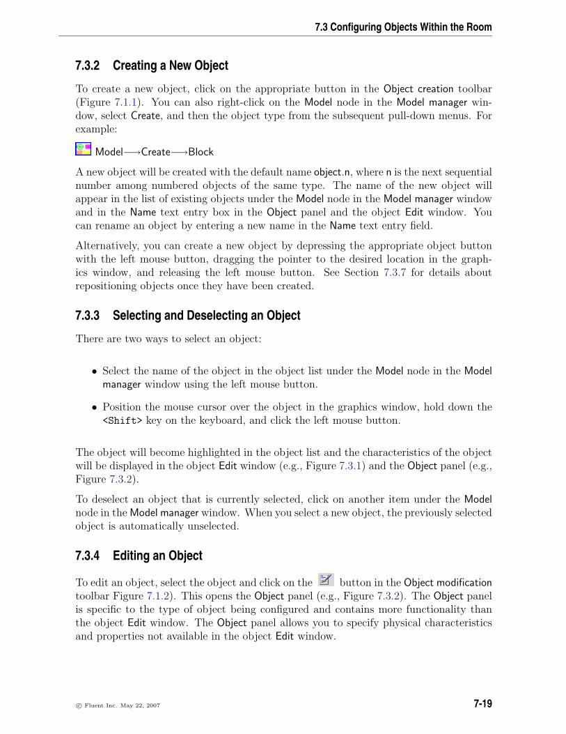
7.3 Configuring Objects Within the Room
7.3.2 Creating a New Object
To create a new object, click on the appropriate button in the Object creation toolbar(Figure 7.1.1). You can also right-click on the Model node in the Model manager win-dow, select Create, and then the object type from the subsequent pull-down menus. Forexample:
Model−→Create−→Block
A new object will be created with the default name object.n, where n is the next sequentialnumber among numbered objects of the same type. The name of the new object willappear in the list of existing objects under the Model node in the Model manager windowand in the Name text entry box in the Object panel and the object Edit window. Youcan rename an object by entering a new name in the Name text entry field.
Alternatively, you can create a new object by depressing the appropriate object buttonwith the left mouse button, dragging the pointer to the desired location in the graph-ics window, and releasing the left mouse button. See Section 7.3.7 for details aboutrepositioning objects once they have been created.
7.3.3 Selecting and Deselecting an Object
There are two ways to select an object:
• Select the name of the object in the object list under the Model node in the Modelmanager window using the left mouse button.
• Position the mouse cursor over the object in the graphics window, hold down the<Shift> key on the keyboard, and click the left mouse button.
The object will become highlighted in the object list and the characteristics of the objectwill be displayed in the object Edit window (e.g., Figure 7.3.1) and the Object panel (e.g.,Figure 7.3.2).
To deselect an object that is currently selected, click on another item under the Modelnode in the Model manager window. When you select a new object, the previously selectedobject is automatically unselected.
7.3.4 Editing an Object
To edit an object, select the object and click on the button in the Object modificationtoolbar Figure 7.1.2). This opens the Object panel (e.g., Figure 7.3.2). The Object panelis specific to the type of object being configured and contains more functionality thanthe object Edit window. The Object panel allows you to specify physical characteristicsand properties not available in the object Edit window.
c© Fluent Inc. May 22, 2007 7-19

Building a Model
i An object must be selected before you click on the button. See Section 7.3.3for details on selecting an object.
Alternate ways of opening the Object panel after selecting an object are as follows:
• Click the Edit button in the object Edit window.
• In the Edit menu, select Current object and then Edit from the subsequent pull-downmenus (Edit−→Current object−→Edit).
• Double-click on the object name in the object list under the Model node in theModel manager window.
• Right-click on the object name under the Model node and select Edit object fromthe pull-down menu.
7.3.5 Deleting an Object
To delete an object, select the object and click on the button in the Object modifi-cation toolbar Figure 7.1.2) or click Delete in the Object panel. The selected object willbe permanently removed from the model and from the list of objects under the Modelnode in the Model manager window.
You can recover a deleted object immediately after the delete operation by selecting Undoin the Edit menu. See Section 2.1.2 for more details on using undo and redo operations.
To remove an object from the model only temporarily, you can deactivate it. See Sec-tion 7.4.1 for details.
Alternate ways of deleting a selected object are as follows:
• Select the object and press the <Delete> key on the keyboard.
• In the Edit menu, select Current object and then Delete from the subsequent pull-down menus (Edit−→Current object−→Delete).
• Right-click on the object name under the Model node and select Delete from thepull-down menu.
7.3.6 Resizing an Object
You can resize an object in Airpak in much the same way as you resize a room. SeeSection 7.2.1 for details on resizing a room. You should note the following differencesbetween resizing an object and resizing a room:
7-20 c© Fluent Inc. May 22, 2007

7.3 Configuring Objects Within the Room
• If you right-click on an object in the list under the Model node and select Moveobject in the pull-down menu, Airpak will open a Move object panel and not theMove all objects in model panel that is used for the room.
• The Autoscale option is not available for objects.
7.3.7 Repositioning an Object
You can reposition an object in Airpak in much the same way as you reposition a room.See Section 7.2.2 for details on repositioning a room. Note that you can also repositionan object (and the room) using a local coordinate system as described on page 7-28.
You should note the following differences between repositioning an object and reposition-ing a room:
• To modify the plane of the currently selected object (if relevant), click the Planetext entry field in the object Edit panel (e.g., Figure 7.3.1) using the left mousebutton to open a list of available planes (yz, xz, and xy), and select a new planefrom the list. The plane of the currently selected object can also be specified inthe Object panel (e.g., Figure 7.3.3) using the Plane drop-down list, where you canchoose Y-Z, X-Z, or X-Y.
• There are several options related to moving an object using the mouse that areavailable for objects but not for the room. These options are displayed in theInteraction section of the Preferences panel (Figure 7.2.7) and are listed below:
X, Y, Z allow you to select which combination of the three axes along which theobject can be translated. For example, if you are positioning an opening on awall, you would want to limit the motion of the opening to only two coordinatedirections in order to move the opening across the surface of the wall.
Restrict movement to room allows you to restrict the motion of the object towithin the room boundaries. If In room is not selected, Airpak will allow theobject to project beyond the room boundaries. This option is on by defaultfor all objects.
Objects can’t penetrate each other instructs Airpak not to allow any penetrationof the object by another object. This option is on by default for all objects.
Move object also moves group allows you to move entire groups using the <Shift>key and the middle mouse button.
Move object snaps to other objects allows you to snap objects to other objectsusing the <Shift> key and the middle mouse button.
Snap Tolerance specifies the distance, in pixels, within which a moved object willbe snapped to another object. When this value has been set, and the modelis oriented in one of the X, Y, or Z views, a dragged object will automatically
c© Fluent Inc. May 22, 2007 7-21

Building a Model
snap into alignment with a second object of similar shape when it comes withinthe specified number of pixels of a vertex, line, or plane of the second object.
New object size factor specifies the default size of a newly-created object in termsof the size of the room. For example, in a 1 m × 1 m × 1 m room, a value of0.2 specifies that new objects will have side lengths of 0.2 m.
i This value does not apply to package objects.
• If you click on the button after selecting an object, Airpak will open a Moveobject panel and not the Move all objects in model panel that is used for the room.You can also open the Move object panel by right-clicking on an object in the listunder the Model node and selecting Move object in the pull-down menu.
If multiple geometric transformations are selected, Airpak applies them in the orderthat they appear in the panel. For example, if both the Rotate and Translateoptions are selected, the new object is rotated first and then translated. Note thatnot all combinations of transformations are commutative; i.e., the result may beorder-dependent, particularly if reflection is used.
If you specify a transformation that moves an object outside the room, Airpak opensthe Objects outside panel (Figure 7.3.6), which contains the following options:
Allow out instructs Airpak to let the object remain outside the room boundary.The object can be either completely outside the room or partly outside theroom, as shown in Figure 7.3.7. This option can be used if the room you havecreated is too small and you want to resize the room at a later time.
Move instructs Airpak to move the object back inside the room. The object ismoved back inside the room as shown in Figure 7.3.8, where the dashed lineshows the position of the object before the move, and the solid line shows theposition of the object after the move.
Resize instructs Airpak to resize the object so that it is inside the room. Airpakwill change the object so that only the part of the object that is inside theroom after the transformation remains in the model, as shown in Figure 7.3.9.The part that is outside will be discarded.
Resize room instructs Airpak to resize the room so that the object is inside theroom, as shown in Figure 7.3.10.
Cancel instructs Airpak to cancel the move operation that caused the object toeither exceed the room dimension or be placed outside the room.
7-22 c© Fluent Inc. May 22, 2007

7.3 Configuring Objects Within the Room
Figure 7.3.6: The Objects outside Panel
c© Fluent Inc. May 22, 2007 7-23

Building a Model
Figure 7.3.7: Object Outside Room Boundary
7-24 c© Fluent Inc. May 22, 2007

7.3 Configuring Objects Within the Room
Figure 7.3.8: Moving the Object Back Inside the Room
c© Fluent Inc. May 22, 2007 7-25

Building a Model
Figure 7.3.9: Resizing an Object that is Outside the Room
7-26 c© Fluent Inc. May 22, 2007

7.3 Configuring Objects Within the Room
Figure 7.3.10: Resizing the Room to Include Outside Object
c© Fluent Inc. May 22, 2007 7-27

Building a Model
Local Coordinate Systems
The global coordinate system has an origin of (0, 0, 0) in Airpak. You can create localcoordinate systems that can be used in your model. The origins of the local coordinatesystems are specified with an offset from the origin of the global coordinate system.
The Local coord systems panel can be used to view and manage all local coordinatesystems in your Airpak model. To open the Local coord systems panel (Figure 7.3.11),double-click on the Local coords item under the Problem setup node in the Model managerwindow.
Problem setup−→ Local coords
Figure 7.3.11: The Local coord systems Panel
The Local coord systems panel can be used to create new local coordinate systems, edit ex-isting local coordinate systems, and delete or deactivate local coordinate systems. Theseoperations are described below.
Each Object panel (e.g., Figure 7.3.3), and also the Room panel (Figure 7.2.3), containsa Local coord system drop-down list. To select a local coordinate system for an object(or for the room), open the Local coord system list and select a local coordinate systemfrom the list. If the Local coord system field is empty, the global coordinate system willbe used for the object (or room).
The Local coord system list can also be used to create a new local coordinate system,edit an existing local coordinate system, and view the definition of the selected localcoordinate system. These operations are described below.
Creating a New Local Coordinate System
To create a new local coordinate system, click on New in the Local coord systems panel(Figure 7.3.11). A new local coordinate system will be created. Rename the local coor-dinate system, if desired. Keep the default Type (Trans), and specify the origin of thelocal coordinate system by entering values for the X offset, Y offset, and Z offset from theorigin of the global coordinate system, which is (0, 0, 0). Repeat these steps to createany other local coordinate systems, and then click Accept.
7-28 c© Fluent Inc. May 22, 2007

7.3 Configuring Objects Within the Room
You can also create a new local coordinate system in any Object panel (or the Roompanel). To create a new local coordinate system, open the Local coord system drop-downlist and select Create new. This will open the Local coords panel (Figure 7.3.12). Entera name in the Name field for the new local coordinate system. Keep the default Type(Trans), and specify the origin of the local coordinate system by entering values for theX offset, Y offset, and Z offset from the origin of the global coordinate system, whichis (0, 0, 0). Click Accept when you have finished creating the local coordinate system,and Airpak will close the Local coords panel and return to the Object panel (or the Roompanel).
Figure 7.3.12: The Local coords Panel
Editing an Existing Local Coordinate System
You can use the Local coord systems panel (Figure 7.3.11) to rename an existing localcoordinate system. You can also change the origin of a local coordinate system byentering new values for the X offset, Y offset, and Z offset from the origin of the globalcoordinate system, which is (0, 0, 0). Click Accept when you have finished editing thelocal coordinate systems.
You can also edit the definition of a local coordinate system in any Object panel (or inthe Room panel). To edit the properties of the local coordinate system selected in theLocal coord system list, open the list and select Edit definition. This will open the Localcoords panel (Figure 7.3.12) and display the properties of the selected coordinate system.You can edit the definition of the coordinate system using the Local coords panel. ClickAccept when you have finished editing the coordinate system, and Airpak will close theLocal coords panel and return to the Object panel (or the Room panel).
i Note that, if you have used a local coordinate system for an object (or the room)and you then edit the origin of the local coordinate system, the position of theobject will not change in the graphics window, because the object’s position withrespect to the global coordinate system is still the same. Because the object isdisplayed with respect to the global coordinate system in the graphics window,
c© Fluent Inc. May 22, 2007 7-29

Building a Model
only its local coordinate values will be adjusted to account for its display location.For example, if the offset values for a local coordinate system were (0.1, 0, 0), thenthe coordinate location of any object using that local coordinate system would beadjusted by -0.1 units in the x direction so that the object is displayed in the samelocation in the graphics window. If the offset values are changed to be (0.2, 0, 0),then the coordinate location of the object(s) would be adjusted by a total of -0.2units in the x direction, but the position of the object in the graphics window (withrespect to the global coordinate system) will still remain the same.
Viewing the Definition of a Local Coordinate System
You can view the definition of a local coordinate system using any Object panel (or theRoom panel). To view the properties of the local coordinate system selected in the Localcoord system list, open the list and select View definition. The Message window will reportthe definition of the coordinate system.
Deleting Local Coordinate Systems
If there are local coordinate systems in the Local coord systems panel (Figure 7.3.11)that you no longer need, you can easily delete them. Click on the Delete button on theline of the coordinate system that you want to delete. The coordinate system will bepermanently removed from your model.
To remove all local coordinate systems from your Airpak model, click Clear in the Localcoord systems panel.
Note that, if you delete a local coordinate system that is being used by an object (or theroom), the object (or room) will remain in the same position in the graphics window.Airpak will add the coordinates of the origin of the local coordinate system to the coor-dinates of the object (or room) and update the coordinates in the Object panel (or theRoom panel) and the object Edit window (or the room Edit window).
Activating and Deactivating Local Coordinate Systems
By default, all local coordinate systems that you create will be available in your currentAirpak model. You can remove a local coordinate system from your model temporarily byturning off the Active option for the coordinate system in the Local coord systems panel(Figure 7.3.11). You can repeat this for each local coordinate system that you want totemporarily remove from your model. When a local coordinate system is deactivated, itis simply removed from the Local coord system drop-down lists, not deleted from Airpak.Since it still exists, you can easily add it to the Local coord system drop-down lists againby turning the Active option back on.
Note that, if you deactivate a local coordinate system that is currently being used byan object (or the room), Airpak will still use the local coordinate system for the object
7-30 c© Fluent Inc. May 22, 2007

7.3 Configuring Objects Within the Room
(or room). Deactivating a local coordinate system only removes it from the Local coordsystem lists so that it cannot be selected.
7.3.8 Aligning an Object With Another Object in the Model
You can align an object with another object in your Airpak model using the Edit windowor the Object modification toolbar.
Aligning Objects With the Object Edit Window
Figure 7.3.13 shows an example of two objects that are close together. To align theright-hand side of object.1 with the left-hand side of object.2 using the object Editwindow, follow the steps below.
Y
X
object.1 object.2
xE=0.6 xS=0.61
Figure 7.3.13: Two Objects That Are Close Together
1. Select the object you want to align (object.1 in this example).
2. In the object Edit window, click on the coordinate that you want to change. Thecoordinates are displayed in orange in the object Edit window. For example, if youwanted to change the xE coordinate of object.1, you would click xE in the objectEdit panel.
3. Use the left mouse button to click on the part of the object that you want to alignyour object with in the graphics window. In this example, you would click on theleft-hand side of object.2.
Airpak will stretch object.1 so that the right-hand side of object.1 coincides with theleft-hand side of object.2.
Aligning Objects With the Object modification Toolbar
You can align an object with another object in your Airpak model in several ways usingthe Object modification toolbar (Figure 7.1.2).
c© Fluent Inc. May 22, 2007 7-31

Building a Model
Aligning Object Faces
You can align two objects with faces that are in parallel planes using the buttonin the Object modification toolbar. Alignment of one object with another using faces canbe accomplished by two methods:
• resizing the selected object by stretching or contracting in the direction normal tothe plane of its selected face, so that the selected face on the chosen object will bein the same plane as the selected face on the reference object
• translating the selected object in the direction normal to the plane of its selectedface, so that the selected face on the chosen object will be in the same plane as theselected face on the reference object
i The resizing option for aligning faces is available only for objects that have prism,cylindrical, or 3D polygon geometries. Objects with these geometries can then beresized only when they are being aligned to objects with similar geometry (e.g.,prism objects cannot be resized to become aligned with cylindrical objects).
To align the faces of two objects, use the following procedure:
1. Decide whether you want to align the two desired objects by resizing or translatingone of the objects.
• To align objects by resizing one of the objects, left-click on the button.
• To align objects by translating one of the objects, right-click on thebutton.
2. Use the left mouse button to select the face of the object that you want to change.If there are multiple faces joined together at the same edge or overlaid on the sameplane, you can cycle through the faces by repeatedly clicking the left button untilthe desired face is selected. If you select the wrong face, click the right mousebutton to deselect it.
3. When you have selected the desired face, click the middle mouse button to acceptthe choice.
4. Repeat steps 2 and 3 for the face on the reference object with which you want thefirst object to be aligned.
7-32 c© Fluent Inc. May 22, 2007

7.3 Configuring Objects Within the Room
Aligning Object Edges
You can align two objects with edges that run in the same direction using the buttonin the Object modification toolbar. Aligning one object to another using edges can beaccomplished by two methods for both 2D and 3D objects:
• 2D objects
– resizing the selected object by stretching (or contracting) in the coordinatedirection normal to the direction of its selected edge, so that the selected edgeof the chosen object will be co-linear with the selected edge on the referenceobject
– translating the selected object in the coordinate direction normal to the di-rection of its selected edge, so that the selected edge of the chosen object willbe co-linear with the selected edge on the reference object
• 3D objects
– resizing the selected object by stretching (or contracting) in up to two co-ordinate directions normal to the direction of its selected edge, so that theselected edge of the chosen object will be co-linear with the selected edge onthe reference object
– translating the selected object in up to two coordinate directions normal tothe direction of its selected edge, so that the selected edge of the chosen objectwill be co-linear with the selected edge on the reference object
i Aligning two objects using edges is not available for objects with circular, cylin-drical, ellipsoid, or elliptical cylinder geometry.
To align the edges of two objects, use the following procedure:
1. Decide whether you want to align the two desired objects by resizing or translatingone of the objects.
• To align objects by resizing one of the objects, left-click on the button.
• To align objects by translating one of the objects, right-click on thebutton.
2. Use the left mouse button to select the edge of the object that you want to change.If there are multiple edges joined together at the same point or overlaid on the sameline, you can cycle through the edges by repeatedly clicking the left button untilthe desired edge is selected. If you select the wrong edge, click the right mousebutton to deselect it.
c© Fluent Inc. May 22, 2007 7-33

Building a Model
3. When you have selected the desired edge, click the middle mouse button to acceptthe choice.
4. Repeat steps 2 and 3 for the edge on the reference object with which you want thefirst object to be aligned.
Figure 7.3.14 shows an example of aligning the edges of two objects using resizing andtranslation.
Figure 7.3.14: Alignment of Two Objects Using Edges
7-34 c© Fluent Inc. May 22, 2007

7.3 Configuring Objects Within the Room
Aligning Object Vertices
You can align two objects by their individual vertices using the button in theObject modification toolbar. Alignment of one object with another using vertices can beaccomplished by two methods:
• resizing the selected object by stretching (or contracting) in up to three coordinatedirections, so that the selected vertex of the chosen object will occupy the samepoint in the room space as the selected vertex on the reference object
• translating the selected object in up to three coordinate directions, so that theselected vertex of the chosen object will occupy the same point in the room spaceas the selected vertex on the reference object
i Aligning two objects using vertices is not available for objects with circular orcylindrical geometry.
To align the vertices of two objects, use the following procedure:
1. Decide whether you want to align the two desired objects by resizing or translatingone of the objects.
• To align objects by resizing one of the objects, left-click on the button.
• To align objects by translating one of the objects, right-click on thebutton.
2. Use the left mouse button to select the vertex of the object that you want to change.If there are multiple vertices occupying the same point, you can cycle through thevertices by repeatedly clicking the left button until the desired vertex is selected.If you select the wrong vertex, click the right mouse button to deselect it.
3. When you have selected the desired vertex, click the middle mouse button to acceptthe choice.
4. Repeat steps 2 and 3 for the vertex on the reference object with which you wantthe first object to be aligned.
Aligning Object Centers
You can align two objects by their geometric centroids using the button in theObject modification toolbar. Alignment of one object to another using centers occurs bytranslating the selected object in up to three coordinate directions so that the center
c© Fluent Inc. May 22, 2007 7-35

Building a Model
of the chosen object will occupy the same point in the room space as the center of thereference object.
To align the centers of two objects, use the following procedure:
1. Left-click on the button.
2. Use the left mouse button to select the object that you want to change. If thereare multiple objects in close proximity to each other, you can cycle through theobjects by repeatedly clicking the left button until the desired object is selected. Ifyou select the wrong object, click the right mouse button to deselect it.
3. When you have selected the desired object, click the middle mouse button to acceptthe choice.
4. Repeat steps 2 and 3 for the reference object with which you want the first objectto be aligned.
Aligning Object Face Centers
You can align two objects by the geometric centers of their faces using the buttonin the Object modification toolbar. Alignment of one object to another using face centersoccurs by translating the selected object in up to three coordinate directions so that thecenter of the face on the chosen object will occupy the same point in the room space asthe center of the face on the reference object.
i Aligning two objects using face centers is not available for objects with ellipsoidgeometry.
To align the face centers of two objects, use the following procedure:
1. Left-click on the button.
2. Use the left mouse button to select the face on the object that you want to change.If there are multiple faces joined together at the same edge or overlaid on the sameplane, you can cycle through the faces by repeatedly clicking the left button untilthe desired face is selected. If you select the wrong face, click the right mousebutton to deselect it.
3. When you have selected the desired face, click the middle mouse button to acceptthe choice.
4. Repeat steps 2 and 3 for the reference object with which you want the first objectto be aligned.
7-36 c© Fluent Inc. May 22, 2007

7.3 Configuring Objects Within the Room
Matching Object Faces
You can align two objects by matching their faces using the button in the Objectmodification toolbar. Alignment of one object to another by matching faces occurs asnecessary by some or all of the following methods:
• resizing the selected object by stretching (or contracting) in one or both of thecoordinate directions of the plane of the selected face
• translating the selected object in up to three coordinate directions
• rotating the selected object so that the plane of the face on the selected object isthe same as the plane of the face on the reference object
i Matching object faces is possible only when the selected faces are being matchedto other object faces with similar geometry. For example, a face on a prism objectcannot be matched to a face on a cylindrical object, but a circular face, such as a2D fan, can be matched to a face on a cylindrical object. Circular faces in differentplanes (e.g., x-y and y-z), however, can not be matched.
i Aligning two objects by matching faces is not available for objects with ellipsoidgeometry.
To align two objects by matching faces, use the following procedure:
1. Left-click on the button.
2. Use the left mouse button to select the face on the object that you want to change.If there are multiple faces joined together at the same edge or overlaid on the sameplane, you can cycle through the faces by repeatedly clicking the left button untilthe desired face is selected. If you select the wrong face, click the right mousebutton to deselect it.
3. When you have selected the desired face, click the middle mouse button to acceptthe choice.
4. Repeat steps 2 and 3 for the reference object with which you want the first objectto be aligned.
c© Fluent Inc. May 22, 2007 7-37

Building a Model
Matching Object Edges
You can align two objects by matching their edges using the button in the Objectmodification toolbar. Alignment of one object to another by matching edges occurs asnecessary by one or both of the following methods:
• resizing the selected object by stretching (or contracting) in the coordinate directionof the selected edge
• translating the selected object in up to three coordinate directions
i Matching object edges is possible only when the selected edges are in the samegeneral plane (i.e., x-y, y-z, x-z, or inclined).
i Aligning two objects by matching edges is not available for objects with circular,cylindrical, ellipsoid, or elliptical cylinder geometry.
To align two objects by matching edges, use the following procedure:
1. Left-click on the button.
2. Use the left mouse button to select the edge on the object that you want to change.If there are multiple edges joined together at the same point or overlaid on the sameline, you can cycle through the edges by repeatedly clicking the left button untilthe desired edge is selected. If you select the wrong edge, click the right mousebutton to deselect it.
3. When you have selected the desired edge, click the middle mouse button to acceptthe choice.
4. Repeat steps 2 and 3 for the reference object with which you want the first objectto be aligned.
7.3.9 Copying an Object
There are two ways to copy an object in Airpak: using the Copy object panel and usingthe Object selection panel.
Copying an Object Using the Copy object Panel
One way to copy an object is to use the Copy object panel. Figure 7.3.15 shows anexample of a Copy object panel specific to copying a block (the Copy block panel). To
open this panel, select the object in the graphics window and click on the buttonin the Object modification toolbar (Figure 7.1.2).
7-38 c© Fluent Inc. May 22, 2007

7.3 Configuring Objects Within the Room
Alternate ways of opening the Copy object panel are as follows:
• In the Edit menu, select Current object and then Copy from the subsequent pull-downmenus (Edit−→Current object−→Copy).
• Right-click on the object name under the Model node and select Copy from thepull-down menu.
i If you copy an object such that the new object is created outside the room, Airpakopens the Objects outside panel, as described in Section 7.3.7.
When you use a Copy object panel, a new object with a sequentially numbered nameappears in the list of existing objects under the Model node in the Model manager window,and the new object appears in the graphics window. Only the options that are selectedin the Copy object panel affect the copy creation.
If multiple geometric transformations are selected, Airpak applies them in the order thatthey appear in the panel. For example, if both the Rotate and Translate options are se-lected, the new object is rotated first and then translated. Note that not all combinationsof transformations are commutative; i.e., the result may be order-dependent, particularlyif reflection is used. If you want to perform a transformation that requires an order ofoperations different from that provided by the Copy object panel, you can create an initialobject and then perform additional transformations in the order desired using the Moveobject panel. See Section 7.3.7 for more information on moving an object.
Options available for copying objects using the Copy object panel include the following:
Number of copies allows you to specify how many copies of the selected object yourequire.
Group name allows you to specify a name for the group to which the new objects willbelong. No group will be created if this option is not selected.
Scale allows you to increase or decrease the size of the new object relative to theoriginal object. To scale the object, turn on the Scale option and specify thescaling factor by entering a value in the Scale text entry box. The scaling factormust be a real number greater than zero. Values greater than 1 will increase thesize, while values less than 1 will decrease the size. To scale the object by differentamounts in different directions, enter the scaling factors separated by spaces. Forexample, if you enter 1.5 2 3 in the Scale text entry box, Airpak will scale theobject by a factor of 1.5 in the x direction, 2 in the y direction, and 3 in the zdirection. To scale the size of multiple copies successively (i.e., to scale the firstcopy relative to the original object, the second copy relative to the first copy, etc.),select Scale copies cumulatively.
c© Fluent Inc. May 22, 2007 7-39
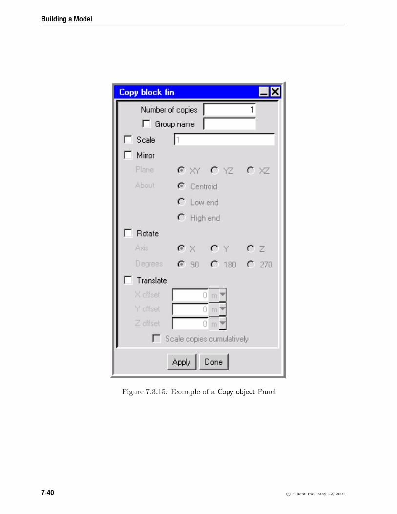
Building a Model
Figure 7.3.15: Example of a Copy object Panel
7-40 c© Fluent Inc. May 22, 2007

7.3 Configuring Objects Within the Room
Mirror allows you to obtain the mirror image of the copied object. To mirror theobject, turn on the Mirror option and specify the Plane across which to reflect theobject by selecting XY, YZ, or XZ. You can also specify the location about whichthe object is to be flipped by selecting Centroid, Low end, or High end next to About.
Rotate allows you to rotate the new object about any coordinate axis from the object’soriginal position. Select X, Y, or Z next to Axis, and then select 90, 180, or 270degrees of rotation.
Translate allows you to translate the new object a specified distance from the originalobject’s position. To translate the new object, turn on Translate and define thedistance of the translation from the current object by specifying an offset in eachof the coordinate directions: X offset, Y offset, and Z offset. If multiple copies arecreated, this translation is relative to the previous copy for each new object.
Copying an Object Using the Object selection Panel
You can also copy an object using the Object selection panel. Figure 7.3.16 shows anexample of an Object selection panel. To open this panel, select Current object and thenCopy from in the Edit menu (e.g., Figure 7.3.1) or click on Copy from in the Object panel(e.g., Figure 7.3.3).
The Copy from option is used when you want to transform an existing object of a specifictype in a particular location into an object of another type in the same location. Consider,for example, that your model includes a block and a resistance and you want to transformthe block into a 3D resistance. In the Resistances panel, click on the Copy from button.This opens the Object selection panel. In the Copy from object list, choose the block.When you click Done, Airpak will create a new object with the location and dimensionsof the block and the physical properties of the resistance.
Other options available in the Object selection panel are as follows:
Deactivate other object deactivates the selected object in the Copy from object list.This option is on by default. The object will be temporarily removed from themodel, which renders the object inactive for purposes of the current analysis.
Delete other object deletes the selected object in the Copy from object list.
Neither does not delete or deactivate the selected object in the Copy from object list.
Copy shape info copies the shape of the object only.
Copy object info copies the shape and the parameters of the object.
Copy creation order ensures that the creation order of the new object is the same asthat selected from the Copy from object list.
c© Fluent Inc. May 22, 2007 7-41

Building a Model
Figure 7.3.16: The Object selection Panel
Copy groups ensures that the new object is put into the same group as the selectedobject in the Copy from object list.
7.4 Object Attributes
When a new object is created in Airpak, default characteristics are applied to the object.Airpak gives the object the following characteristics, which are displayed in the objectEdit window or the Object panel, or, in some cases, in both places.
• Description (name, notes, group, include or exclude the object)
• Graphical style (shading, line width, color, texture, transparency)
• Position and size
• Geometry
• Physical characteristics
7-42 c© Fluent Inc. May 22, 2007

7.4 Object Attributes
The first four characteristics relate to all objects and are described below. The physicalcharacteristics are specific to a particular object and are described in detail in the chapterrelated to that object.
7.4.1 Description
Airpak allows you to change the name of the object, specify the group to which it belongs,and include or exclude the object. These options are described below.
Changing the Name of an Object
Airpak allows you to change the name of an object. The name of an object is displayed inthe Name text entry box in the object Edit window (e.g., Figure 7.3.1) and in the Nametext entry box in the Object panel (e.g., Figure 7.3.2). To change the name of an object,enter a new name in the Name text entry box.
Adding Notes About the Object
You can enter notes for object under Notes for this object in the Notes tab of the Roompanel (e.g., Figure 7.3.5). There is no restriction on the number and type of text charac-ters you can use. When you are finished entering or updating the text in this field, clickUpdate to store this information along with the object.
Assigning an Object to a Group
The group to which the object belongs is displayed in the Group text entry box in theobject Edit window (e.g., Figure 7.3.1) and in the Groups text entry box in the Objectpanel (e.g., Figure 7.3.2). You can specify the group to which the object belongs (ifapplicable) by entering the name of the group in the Group text entry box.
Including or Excluding an Object
You can include an object in the model or exclude it by selecting or deselecting Activein the Object panel (e.g., Figure 7.3.2). The object is included by default. If the Activeoption is deselected, the object is temporarily removed from the model, which rendersthe object inactive for purposes of the current analysis.
7.4.2 Graphical Style
Airpak allows you to change the display of the object in the graphics window. Theprocedure for changing the color and line width of the object is the same as for changingthe color and line width of the room, as described in Section 7.2.5.
c© Fluent Inc. May 22, 2007 7-43

Building a Model
Changing the Shading
The Shading of an object in the graphics window is shown as default in the Object panel(e.g., Figure 7.3.2). The type of shading that will be applied to the object when defaultis selected is defined in the Object types section of the Preferences panel (see Section 6.3.6for more details on changing the default shading using the Preferences panel). To changethe shading of the object, click on the square button to the right of the Shading text fieldin the Object panel. Select a shading type in the resulting drop-down list: default, Wire,Solid, Solid/wire, Hidden line, or Invisible. Click Update at the bottom of the Object panelto change the shading for the object in the graphics window.
Changing the Texture
The Texture of an object in the graphics window can be modified when Solid or Solid/wirehas been selected in the Shading drop-down list. The default texture option is No texture.To modify the texture, select Load from file and select an available PPM image file in theresulting File selection dialog box (see Section 2.1.8).
Depending on its pixel size, the image, or a portion thereof, will be used to cover eachside of the object. To change the size of the image used for the texture, specify a valuefor the Texture scale. Values greater than 1.0 will reduce the size of the image on eachside of the object, resulting in a tiling effect at large enough values. Values less than 1.0will increase the size of the image on each side of the object.
Changing the Transparency
The transparency of an object in the graphics window can be modified by turning on theTransparency option and moving the slider bar between values of 0.00 (opaque) and 0.99(fully transparent). This option is useful when Solid has been selected in the Shadingdrop-down list.
7.4.3 Position and Size
An example of how Airpak displays the position and size of an object is described belowfor a rectangular object.
• The plane of the currently selected object is displayed in the object Edit window(e.g., Figure 7.3.1) next to Plane (if relevant). For 2D objects, Plane is the planethe object is in. (For 3D objects, Plane is not available.) To modify the plane,select a new plane in the drop-down list of available planes (yz, xz, and xy). Theplane of the currently selected object can also be specified in the Object panel (e.g.,Figure 7.3.3) by selecting Y-Z, X-Z, or X-Y in the Plane drop-down list.
• The starting and ending points of the selected object are displayed in the objectEdit window (e.g., Figure 7.3.1) and in the Object panel (e.g., Figure 7.3.3) under
7-44 c© Fluent Inc. May 22, 2007

7.4 Object Attributes
Location if Start/end is selected. For rectangular objects, the start and end pointstake the form (xS, yS, zS) and (xE, yE, zE). If Start/length is selected in the Objectpanel or the object Edit window, the starting point of the object (xS, yS, zS) andthe lengths of the sides (xL, yL, and zL) are displayed in the Object panel and theobject Edit window.
7.4.4 Geometry
Airpak displays the geometry of the currently selected object in the object Edit window(e.g., Figure 7.3.1) next to Geom. To modify the geometry, select a new geometry fromthe list of available geometries. The geometries available depend on the type of objectselected. For example, the geometries available for a block are prism, cylinder, polygon,ellipsoid, and elliptical cylinder. The geometry of the currently selected object can alsobe specified in the Object panel (e.g., Figure 7.3.3) in the Shape drop-down list.
The geometries available in Airpak are listed below and described in the following sections.
• rectangular
• circular
• inclined
• polygon (2D and 3D)
• prism
• cylindrical
• ellipsoid
• elliptical cylinder
• CAD
Rectangular Objects
The location and dimension parameters for a rectangular object include the coordinateplane (Y-Z, X-Y, or X-Z) in which the object lies and its physical dimensions. A rectan-gular object is defined by the coordinates of its lower left and upper right corners (seeFigure 7.4.1). These are referred to as the starting point (xS, yS, zS) and ending point(xE, yE, zE), respectively. The coordinate on the axis that is normal to the plane of theobject is specified only for the starting point. For the ending point, this same value isused. For example, if the object is in the X-Z plane, you specify xS, yS, zS, xE, and zE,and Airpak automatically sets yE equal to yS.
Rectangular geometries are available for the following objects:
c© Fluent Inc. May 22, 2007 7-45

Building a Model
(xS, yS, zS)
(xE, yE, zE)
X
Y
Z
Figure 7.4.1: Rectangular Object Definition
• fans
• vents
• openings
• persons (faces)
• walls
• partitions
• sources
• resistances
• hoods (flanges, exhausts)
To specify a rectangular object, select Rectangular in the Shape drop-down list in theObject panel. The user inputs for a rectangular object are shown below.
7-46 c© Fluent Inc. May 22, 2007

7.4 Object Attributes
Select the plane in which the object lies (Y-Z, X-Z, or X-Y) in the Plane drop-down list.Select Start/end in the Specify by drop down list and enter values for the start coordinates(xS, yS, zS) and end coordinates (xE, yE, zE) of the object, or select Start/length and entervalues for the start coordinates (xS, yS, zS) and lengths of the sides (xL, yL, and zL) ofthe object.
Circular Objects
A circular object (see Figure 7.4.2) is defined by the coordinate location of its center (xC,yC, zC), the plane (X-Y, Y-Z, or X-Z) in which the object lies, and its Radius.
(xC, yC, zC)
Radius
XY
Z
Figure 7.4.2: Circular Object Definition
Circular geometries are available for the following objects:
• fans
• vents
• openings
• walls
• partitions
• sources
• resistances
To specify a circular object, select Circular in the Shape drop-down list in the Objectpanel. The user inputs for a circular object are shown below.
c© Fluent Inc. May 22, 2007 7-47

Building a Model
Specify the location of the center of the object (xC, yC, zC), the plane in which the objectlies (Y-Z, X-Z, or X-Y), and the Radius of the object. For a circular fan, you can specifythe size of the hub or inner radius (IRadius).
You can also define a circular object on the surface of another circular object. Forexample, you can create a circular fan on the circular face of a cylindrical block. Usethe Orient menu or the Orientation commands toolbar to specify the desired orientationof the object. For the cylindrical block, you would choose the orientation such that thecircular face of the block is in the plane of the graphics window. Then, for the fan, selectCircular in the drop-down list next to Geom in the fan Edit window and click on Select3 points. Using the left mouse button, select the first, second, and third points on theradius of the circular face of the cylindrical block in the graphics window. For a circularfan, you can also specify the size of the hub or inner radius by selecting an inner radiuspoint in the graphics window using the left mouse button.
Inclined Objects
An inclined object has only two of its edges aligned with a coordinate axis (X, Y, orZ), and its physical dimensions are defined by the coordinates of a rectangular box thatserves as its boundary (see Figure 7.4.3). The lower left corner and upper right corner ofthe box are referred to as the starting point (xS, yS, zS) and ending point (xE, yE, zE),respectively.
To complete the definition of an inclined object, you must specify the axis around whichit is rotated and the orientation of the object (see Figure 7.4.4).
Inclined geometries are available for the following objects:
• fans
• vents
• openings
• walls
7-48 c© Fluent Inc. May 22, 2007

7.4 Object Attributes
Figure 7.4.3: Inclined Object Definition
Figure 7.4.4: Inclined Object Slope Definition
c© Fluent Inc. May 22, 2007 7-49

Building a Model
• partitions
• sources
• resistances
To specify an inclined object, select Inclined in the Shape drop-down list in the Objectpanel. The user inputs for an inclined object are shown below.
Specify the Axis of rotation by selecting X, Y, or Z in the drop-down list. Under Location,select one of the following options from the Specify by drop-down list to specify thelocation of the inclined object.
Start/end Enter values for the start coordinates (xS, yS, zS) and end coordinates (xE,yE, zE), and specify the Orientation by selecting Positive or Negative in the drop-down list.
Start/length Enter values for the start coordinates (xS, yS, zS) and lengths of the sides(xL, yL, and zL) of the object, and specify the Orientation by selecting Positive orNegative in the drop-down list.
Start/angle Enter values for the start coordinates (xS, yS, zS) and lengths of the sides(xL, yL, and zL) of the object, and specify the Angle of inclination of the object.
Polygon Objects
Two-dimensional polygons and three-dimensional polygons are available in Airpak.
7-50 c© Fluent Inc. May 22, 2007
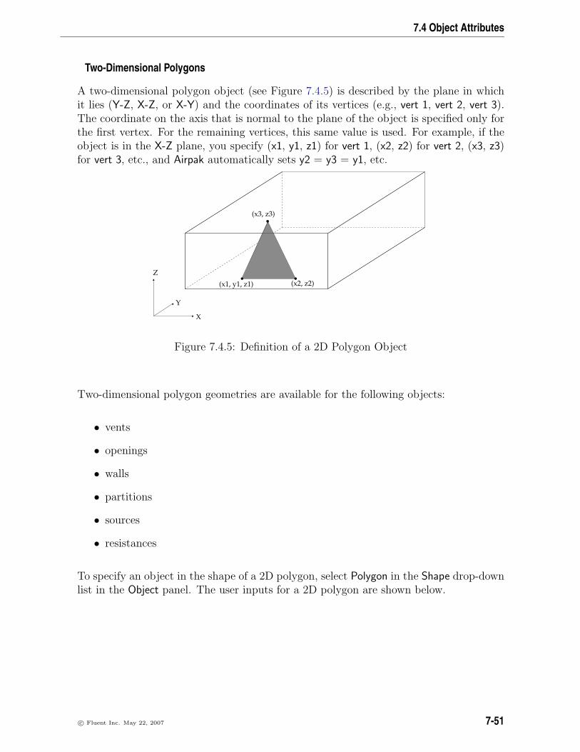
7.4 Object Attributes
Two-Dimensional Polygons
A two-dimensional polygon object (see Figure 7.4.5) is described by the plane in whichit lies (Y-Z, X-Z, or X-Y) and the coordinates of its vertices (e.g., vert 1, vert 2, vert 3).The coordinate on the axis that is normal to the plane of the object is specified only forthe first vertex. For the remaining vertices, this same value is used. For example, if theobject is in the X-Z plane, you specify (x1, y1, z1) for vert 1, (x2, z2) for vert 2, (x3, z3)for vert 3, etc., and Airpak automatically sets y2 = y3 = y1, etc.
(x1, y1, z1) (x2, z2)
X
Y
Z
(x3, z3)
Figure 7.4.5: Definition of a 2D Polygon Object
Two-dimensional polygon geometries are available for the following objects:
• vents
• openings
• walls
• partitions
• sources
• resistances
To specify an object in the shape of a 2D polygon, select Polygon in the Shape drop-downlist in the Object panel. The user inputs for a 2D polygon are shown below.
c© Fluent Inc. May 22, 2007 7-51
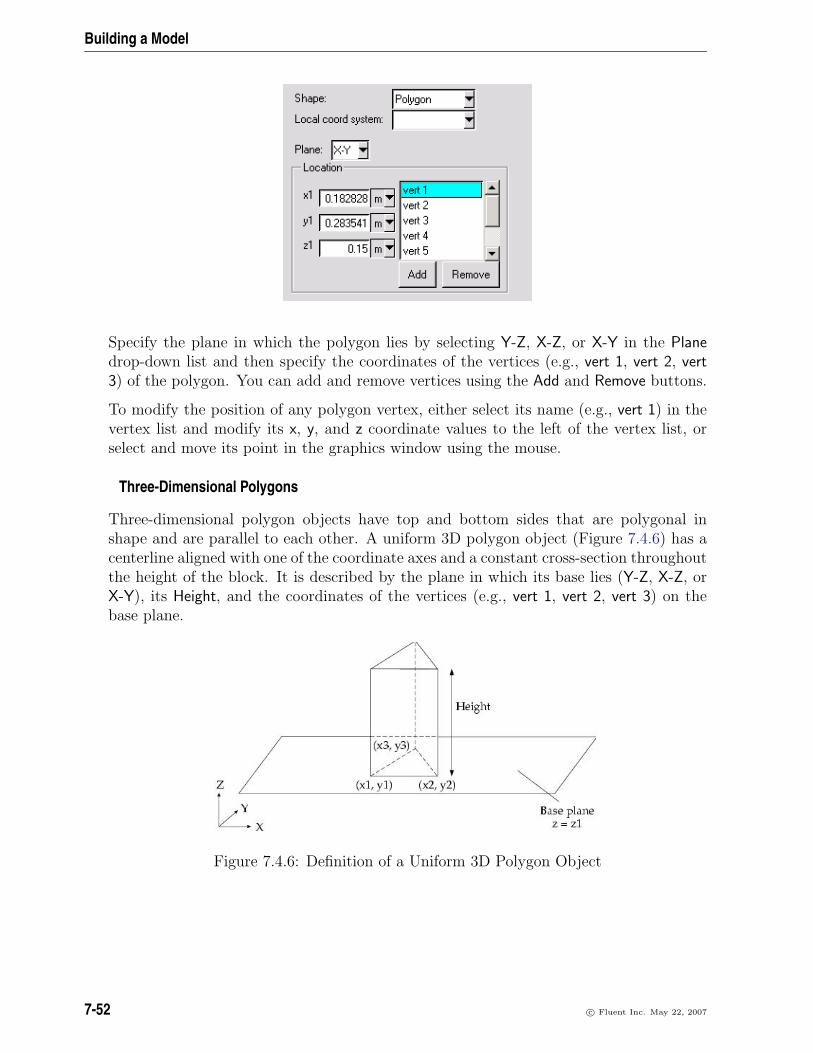
Building a Model
Specify the plane in which the polygon lies by selecting Y-Z, X-Z, or X-Y in the Planedrop-down list and then specify the coordinates of the vertices (e.g., vert 1, vert 2, vert3) of the polygon. You can add and remove vertices using the Add and Remove buttons.
To modify the position of any polygon vertex, either select its name (e.g., vert 1) in thevertex list and modify its x, y, and z coordinate values to the left of the vertex list, orselect and move its point in the graphics window using the mouse.
Three-Dimensional Polygons
Three-dimensional polygon objects have top and bottom sides that are polygonal inshape and are parallel to each other. A uniform 3D polygon object (Figure 7.4.6) has acenterline aligned with one of the coordinate axes and a constant cross-section throughoutthe height of the block. It is described by the plane in which its base lies (Y-Z, X-Z, orX-Y), its Height, and the coordinates of the vertices (e.g., vert 1, vert 2, vert 3) on thebase plane.
Figure 7.4.6: Definition of a Uniform 3D Polygon Object
7-52 c© Fluent Inc. May 22, 2007

7.4 Object Attributes
A non-uniform 3D polygon object (Figure 7.4.7) can be skewed with respect to thecoordinate axes and can possess top and bottom sides of different shapes. It is describedby the plane in which its base lies (Y-Z, X-Z, or X-Y), its Height, and the coordinates ofits vertices (e.g., low 1, low 2, low 3, high 1, high 2, high 3). The top and bottom sides ofa non-uniform 3D polygon object can differ in shape but must be parallel to each otherand possess an identical number of vertices.
Figure 7.4.7: Definition of a Non-Uniform 3D Polygon Object
Three-dimensional polygon geometries are available for the following objects:
• blocks
• fans
• openings (recirculation only)
• hoods (canopy)
To specify an object in the shape of a 3D polygon, select Polygon in the Shape drop-downlist in the Object panel. The user inputs for a 3D polygon are shown below.
c© Fluent Inc. May 22, 2007 7-53

Building a Model
For a uniform 3D polygonal object, specify the plane in which the base lies by selectingY-Z, X-Z, or X-Y in the Plane drop-down list. Under Location, specify the Height and thecoordinates of the vertices (e.g., vert 1, vert 2, vert 3) on the base plane. You can addand remove vertices using the Add and Remove buttons.
If you select None in the Plane drop-down list, the polygonal block will be constructedwith zero height and will take the shape of the base of the polygon.
For a non-uniform 3D polygon object, select Nonuniform and specify the plane in whichthe base lies by selecting Y-Z, X-Z, or X-Y in the Plane drop-down list. Under Locationspecify the Height and the coordinates of its vertices (e.g., low 1, low 2, low 3, high 1, high2, high 3).
For a uniform 3D polygon object, the top and bottom sides are identical in shape andsize, and the cross-section is uniform in one coordinate direction. (Therefore, a uniform3D polygon object is completely defined by its height and the coordinates of its basevertices.) In a non-uniform 3D polygon object, the top and bottom sides lie in parallelplanes and possess an identical number of vertices but are not identical in shape orsize. Also, their centroids do not necessarily lie along a line parallel to any one of thecoordinate axes.
The default 3D polygon object is uniform in type with a triangular base and a Height of0.2 m. To modify the position of any polygon vertex, either select its name (e.g., vert 1or low 2) in the vertex list and modify its x, y, and z coordinate values to the left of thevertex list, or select and move its point in the graphics window using the mouse.
i The mouse operations for a 3D polygon object in the graphics window do notrestrict you from specifying vertices that render the top and bottom sides of theobject non-parallel. However, Airpak’s meshing procedures are not designed tomesh such shapes. To prevent the accidental creation of an unmeshable 3D polygon
7-54 c© Fluent Inc. May 22, 2007

7.4 Object Attributes
object, restrict allowable point movement in the graphics window (using the Motionallowed toggle buttons in the Interactive editing panel as described in Section 7.3.7)before selecting and moving the polygon vertices.
Prism Objects
A prism object (Figure 7.4.8) has its sides aligned with the three coordinate planes. Itslocation is defined by the coordinates of the lower left front corner, referred to as theobject starting point (xS, yS, zS), and the upper right corner, referred to as the objectending point (xE, yE, zE).
Figure 7.4.8: Definition of a Prism Object
Prism geometries are available for the following objects:
• blocks
• persons (head, body, arms, legs, thighs)
• sources
• resistances
• hoods (neck)
To specify an object in the shape of a prism, select Prism in the Shape drop-down list inthe Object panel. The user inputs for a prism are shown below.
c© Fluent Inc. May 22, 2007 7-55

Building a Model
Under Specify by, select Start/end and enter values for the start coordinates (xS, yS, zS)and end coordinates (xE, yE, zE) of the prism object, or select Start/length and entervalues for the start coordinates (xS, yS, zS) and lengths of the sides (xL, yL, and zL) ofthe prism object.
Cylindrical Objects
Cylindrical objects can be specified as uniform or non-uniform. A uniform cylindricalobject (Figure 7.4.9) has a constant radius throughout the height of the object, and canbe described by its Radius, Height, the plane in which its base lies (Y-Z, X-Z, or X-Y),and the location of the center of its base (xC, yC, zC).
Figure 7.4.9: Definition of a Uniform Cylindrical Object
A non-uniform cylindrical object (Figure 7.4.10) has a radius that varies linearly withobject height, and can be described by the parameters specified for a uniform cylinderand by the radius of the top of the cylinder (the side not located on the base plane).
Concentric cylinders are defined by the plane in which the circular base lies (X-Y, Y-Z, orX-Z), the outer radius of the cylinder (Radius), the inner radius (Int Radius), the coordi-nates of the center of the base (xC, yC, zC), and the height of the cylinder. Additionally,
7-56 c© Fluent Inc. May 22, 2007

7.4 Object Attributes
Figure 7.4.10: Definition of a Non-Uniform Cylindrical Object
the Nonuniform radius option can be enabled so that the cylinder can have varying radiusalong the length of its internal or external surfaces. The direction of increasing height isthe normal direction to the specified plane. For example, if the circular base lies in theX-Z plane, the height will increase in the y direction.
Cylindrical geometries are available for the following objects:
• blocks
• fans
• openings (recirculation only)
• sources
• resistances
To specify an object in the shape of a cylinder, select Cylinder in the Shape drop-downlist in the Object panel. The user inputs for a cylinder are shown below.
c© Fluent Inc. May 22, 2007 7-57
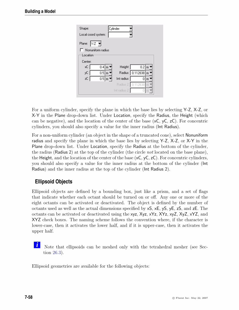
Building a Model
For a uniform cylinder, specify the plane in which the base lies by selecting Y-Z, X-Z, orX-Y in the Plane drop-down list. Under Location, specify the Radius, the Height (whichcan be negative), and the location of the center of the base (xC, yC, zC). For concentriccylinders, you should also specify a value for the inner radius (Int Radius).
For a non-uniform cylinder (an object in the shape of a truncated cone), select Nonuniformradius and specify the plane in which the base lies by selecting Y-Z, X-Z, or X-Y in thePlane drop-down list. Under Location, specify the Radius at the bottom of the cylinder,the radius (Radius 2) at the top of the cylinder (the circle not located on the base plane),the Height, and the location of the center of the base (xC, yC, zC). For concentric cylinders,you should also specify a value for the inner radius at the bottom of the cylinder (IntRadius) and the inner radius at the top of the cylinder (Int Radius 2).
Ellipsoid Objects
Ellipsoid objects are defined by a bounding box, just like a prism, and a set of flagsthat indicate whether each octant should be turned on or off. Any one or more of theeight octants can be activated or deactivated. The object is defined by the number ofoctants used as well as the actual dimensions specified by xS, xE, yS, yE, zS, and zE. Theoctants can be activated or deactivated using the xyz, Xyz, xYz, XYz, xyZ, XyZ, xYZ, andXYZ check boxes. The naming scheme follows the convention where, if the character islower-case, then it activates the lower half, and if it is upper-case, then it activates theupper half.
i Note that ellipsoids can be meshed only with the tetrahedral mesher (see Sec-tion 26.3).
Ellipsoid geometries are available for the following objects:
7-58 c© Fluent Inc. May 22, 2007

7.4 Object Attributes
• blocks
• sources
To specify an object in the shape of an ellipsoid, select Ellipsoid in the Shape drop-downlist in the Object panel. The user inputs for an ellipsoid are shown below.
Under Location, specify the dimensions of the object (xS, xE, yS, yE, zS, zE). UnderCorners, activate or deactivate octants by selecting or deselecting xyz, Xyz, xYz, XYz, xyZ,XyZ, xYZ, or XYZ. The naming scheme follows the convention where, if the character islower-case, then it activates the lower half, and if it is upper-case, then it activates theupper half.
Elliptical Cylinder Objects
Elliptical cylinders (E. cylinder) are defined with four quadrants. The two centers arespecified by X, Y, Z for the bottom center point (Bot cent), and X, Y, Z for the top center(Top cent), as shown in Figures 7.4.11 and 7.4.12. Each center has two vectors thatshould be perpendicular, which define the two end caps of the cylinder. The four vectorsare named Bot vec 1 and Bot vec 2 for the low center (Bot cent), and Top vec 1 and Topvec 2 for the high center (Top cent). One or more of the quadrants can be activated ordeactivated using the check buttons -1 -2, -1 +2, +1 -2, and +1 +2. Here, -1 -2 is thequadrant between the vectors -Bot vec 1 and -Bot vec 2, -1 +2 is the quadrant betweenthe vectors -Bot vec 1 and Bot vec 2, +1 -2 is the quadrant between the vectors Bot vec1 and -Bot vec 2, and +1 +2 is the quadrant between the vectors Bot vec 1 and Bot vec2.
i Note that elliptical cylinders can be meshed only with the tetrahedral mesher (seeSection 26.3).
c© Fluent Inc. May 22, 2007 7-59

Building a Model
Bottom radius
Bottom int radius
(X,Y,Z)
Top radius (X,Y,Z)
Top int radius
Quadrant +1−2
Quadrant −1−2
Quadrant +1+2
Quadrant −1+2
Bottom
Top
Y
X
Z
Figure 7.4.11: Nomenclature for Simplified Elliptical Cylinders
7-60 c© Fluent Inc. May 22, 2007

7.4 Object Attributes
Figure 7.4.12: Nomenclature for Detailed Elliptical Cylinders
c© Fluent Inc. May 22, 2007 7-61

Building a Model
Elliptical cylinder geometries are available for the following objects:
• blocks
• sources
To specify an object in the shape of an elliptical cylinder, select E. cylinder in the Shapedrop-down list in the Object panel. The user inputs for an elliptical cylinder are shownbelow.
Specify X, Y, Z for the bottom center point (Bot cent), and X, Y, Z for the top centerpoint (Top cent).
The Simplified specification option allows you to define a cylinder with circular end capsof variable radius and also allows you to define tube-like geometry. For the Simplifiedspecification, specify the Bot radius and Bot int radius for the bottom end cap, and theTop radius and Top int radius for the top end cap.
The Detailed specification allows you to define an elliptical cylinder with non-parallel endcaps, because the vectors can encompass all three coordinate directions. For the Detailedspecification, specify perpendicular vectors for the bottom center (Bot vec 1 and Bot vec2) and for the top center (Top vec 1 and Top vec 2).
When you have specified the necessary radii or vectors, activate or deactivate quadrantsby selecting or deselecting -1 -2, -1 +2, +1 -2, and +1 +2 next to Corners. For the Detailedspecification, -1 -2 is the quadrant between the vectors -Bot vec 1 and -Bot vec 2, -1 +2 isthe quadrant between the vectors -Bot vec 1 and Bot vec 2, +1 -2 is the quadrant between
7-62 c© Fluent Inc. May 22, 2007

7.4 Object Attributes
the vectors Bot vec 1 and -Bot vec 2, and +1 +2 is the quadrant between the vectorsBot vec 1 and Bot vec 2. For the Simplified specification, the four quadrants (Corners) aredefined in the same way as for a detailed elliptical cylinder if you imagine that setting avalue for the Bot radius is equivalent to setting Bot vec 1 and Bot vec 2 to be the samelength and in the same plane.
CAD Objects
CAD objects are directly imported using the IGES/STEP import feature (see Sec-tion 4.2). CAD objects can possess the most general 2D (Figure 7.4.13) and 3D (Fig-ure 7.4.14) shapes. The geometry of a CAD object cannot be specified or modified inAirpak. As such, any changes to the shape of the object must be made in the CAD toolbefore being exported as an IGES/Step file.
z
xy
Figure 7.4.13: 2D CAD Object
i CAD geometries are available only for blocks and partitions.
7.4.5 Physical Characteristics
Airpak allows you to specify the physical characteristics of an object in the Object panel(e.g., Figure 7.3.4). The physical characteristics are specific to the type of object beingconfigured. For example, the Object panel for printed circuit boards allows you to specifywhether there is a rack of boards, and, if so, how many boards are in the rack. Also, youcan specify the number and height of components on each side of the board, as well as
c© Fluent Inc. May 22, 2007 7-63
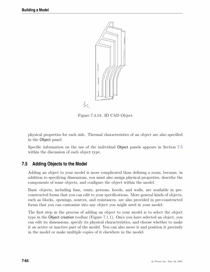
Building a Model
Figure 7.4.14: 3D CAD Object
physical properties for each side. Thermal characteristics of an object are also specifiedin the Object panel.
Specific information on the use of the individual Object panels appears in Section 7.5within the discussion of each object type.
7.5 Adding Objects to the Model
Adding an object to your model is more complicated than defining a room, because, inaddition to specifying dimensions, you must also assign physical properties, describe thecomponents of some objects, and configure the object within the model.
Basic objects, including fans, vents, persons, hoods, and walls, are available in pre-constructed forms that you can edit to your specifications. More general kinds of objects,such as blocks, openings, sources, and resistances, are also provided in pre-constructedforms that you can customize into any object you might need in your model.
The first step in the process of adding an object to your model is to select the objecttype in the Object creation toolbar (Figure 7.1.1). Once you have selected an object, youcan edit its dimensions, specify its physical characteristics, and choose whether to makeit an active or inactive part of the model. You can also move it and position it preciselyin the model or make multiple copies of it elsewhere in the model.
7-64 c© Fluent Inc. May 22, 2007

7.6 Grouping Objects
The basic steps for adding an object to your model are as follows:
1. Create the object.
2. Change the description of the object.
3. Change the graphical style of the object (optional).
4. Specify the geometry, position, and size of the object.
5. Specify the type of the object (if relevant).
6. Specify the physical and thermal characteristics of the object.
The objects available for your Airpak model are described in detail in the Chapters 8–19.
7.6 Grouping Objects
Airpak allows you to group objects in your model. Groups can be used for several pur-poses, including the following:
• defining a set of objects as a single design element so that you can use it repeatedlyin a series of models
• modifying the properties of like objects
• designating a collection of objects as a set to test one part of the model indepen-dently from the whole model
• moving several objects simultaneously
• grouping objects together for postprocessing purposes
• turning defined sets of objects on and off at your discretion
Groups can be easily activated and deactivated, allowing you to control the parts of yourmodel at a sub-assembly level by selecting the objects that are to be included in thecurrent analysis. Groups can be copied or moved within the model using a variety ofgeometric transformations. Airpak allows you to copy the properties of one object to acollection of objects of the same type in a single operation.
You can use the Edit menu or the Groups node in the Model manager window (Figure 7.6.1)to create and configure groups within your Airpak model.
Edit−→Current group
The procedures for creating and configuring groups are described in the following sections.
c© Fluent Inc. May 22, 2007 7-65

Building a Model
Figure 7.6.1: The Groups Node in the Model manager Window
7-66 c© Fluent Inc. May 22, 2007

7.6 Grouping Objects
7.6.1 Creating a Group
To create a new group, double-click on the Groups node in the Model manager window(Figure 7.6.1) or select Create in the Edit−→Current group menu. The new group nodewill be added under the Groups node. It will not contain any objects until you add themto it, as described in Section 7.6.4.
Alternatively, you can use the <Control> and <Shift> keys in combination with themouse to select multiple objects in the Model manager window (see Section 2.2.2). Tocreate a group from the selected items, right-click on one of the items and select Creategroup in the pull-down menu. In the resulting Query dialog box (Figure 7.6.2), enter aname and click Done.
Figure 7.6.2: The Query Dialog Box for Creating a Group
Airpak will create a new group with the default name group.n, where n is the next se-quential number among numbered groups. The Groups node lists the groups that alreadyexist in the current model. Selecting a group in this list and expanding the node willdisplay the list of objects it contains.
7.6.2 Renaming a Group
To rename an existing group, right-click on the group node in the Model manager win-dow (Figure 7.6.1) and select Rename in the pull-down menu or select Rename in theEdit−→Current group menu. In the resulting Query dialog box (Figure 7.6.3), enter a newname and click Done.
Figure 7.6.3: The Query Dialog Box for Renaming a Group
c© Fluent Inc. May 22, 2007 7-67
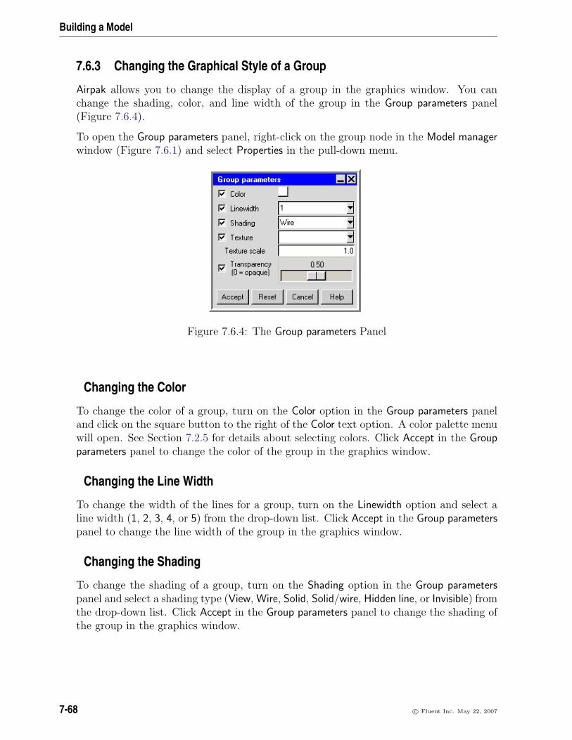
Building a Model
7.6.3 Changing the Graphical Style of a Group
Airpak allows you to change the display of a group in the graphics window. You canchange the shading, color, and line width of the group in the Group parameters panel(Figure 7.6.4).
To open the Group parameters panel, right-click on the group node in the Model managerwindow (Figure 7.6.1) and select Properties in the pull-down menu.
Figure 7.6.4: The Group parameters Panel
Changing the Color
To change the color of a group, turn on the Color option in the Group parameters paneland click on the square button to the right of the Color text option. A color palette menuwill open. See Section 7.2.5 for details about selecting colors. Click Accept in the Groupparameters panel to change the color of the group in the graphics window.
Changing the Line Width
To change the width of the lines for a group, turn on the Linewidth option and select aline width (1, 2, 3, 4, or 5) from the drop-down list. Click Accept in the Group parameterspanel to change the line width of the group in the graphics window.
Changing the Shading
To change the shading of a group, turn on the Shading option in the Group parameterspanel and select a shading type (View, Wire, Solid, Solid/wire, Hidden line, or Invisible) fromthe drop-down list. Click Accept in the Group parameters panel to change the shading ofthe group in the graphics window.
7-68 c© Fluent Inc. May 22, 2007

7.6 Grouping Objects
Note that the type of shading that will be applied to the group when View is selected istaken from the Shading sub-menu in the View menu, described in Section 2.1.2.
Changing the Texture
The surface texture of a group can be modified when Solid or Solid/wire has been selectedin the Shading drop-down list. The default texture option is No texture. To modify thetexture, turn on the Texture option in the Group parameters panel . Select Load from file,and then select an available PPM image file in the resulting File selection dialog box (seeSection 2.1.8).
Depending on its pixel size, the image, or a portion thereof, will be used to cover eachside of the object. To change the size of the image used for the texture, specify a valuefor the Texture scale. Values greater than 1.0 will reduce the size of the image on eachside of the object, resulting in a tiling effect at large enough values. Values less than 1.0will increase the size of the image on each side of the object.
Changing the Transparency
The transparency of a group can be modified by turning on the Transparency option andmoving the slider bar between values of 0.00 (opaque) and 0.99 (fully transparent). Thisoption is most useful when Solid has been selected in the Shading drop-down list.
7.6.4 Adding Objects to a Group
To add an object to a group, right-click on the group node in the Model manager win-dow (Figure 7.6.1) and select Add in the pull-down menu or select Add to group in theEdit−→Current group menu.
There are three ways to add objects to a group using these menus:
Screen select adds individually selected objects to a group. To add an object to agroup, select Screen select and then use the <Shift> key and the left mouse buttonto select the object you want to add to the group in the graphics window. Todeactivate the Screen select mode, press the <Shift> key and click the middlemouse button or the right mouse button in the graphics window.
Screen region adds objects to a group based on their location in the model. Thisoption allows you to add all objects in an entire region of the model to a group.To add objects, select Screen region and then select the objects in the model to beadded to the group by defining a rectangular box on the screen. Position the mousepointer at a corner of the area where the objects to be included are located, holddown the left mouse button and drag open a selection box to enclose the objects tobe included, and then release the mouse button. The objects within the boundedarea will be added to the currently-selected group.
c© Fluent Inc. May 22, 2007 7-69

Building a Model
Name/pattern adds any object whose name matches a specified text pattern to agroup. To add an object, select Name/pattern. This opens a Query dialog box(Figure 7.6.5).
Figure 7.6.5: The Query Dialog Box for Adding Objects to a Group
You can type an object name that contains an asterisk or a question mark in placeof characters or a character, respectively. For example, typing fan* will add allobjects whose names start with fan to the group; typing vent? will add all objectswhose names consist of the word vent plus one character to the group. Any objectin the model whose name matches this text pattern will be added to the groupwhen you click Done in the Query dialog box.
You can also add an object to a group by typing the name of the group in the Groupstext entry box in the Object panel (see Section 7.4.1).
7.6.5 Removing Objects From a Group
To remove an object from a group, right-click on the group node in the Model managerwindow (Figure 7.6.1) and select Remove in the pull-down menu or select Remove fromgroup in the Edit−→Current group menu.
There are three ways to remove objects from a group using these menus. For all methods,the object(s) will be removed only from the group, not from the model.
Screen select removes individually selected objects from an existing group. To removean object from a group, select Screen select and use the <Shift> key and the leftmouse button to select the object you want to remove from the group in the graphicswindow. To deactivate the Screen select mode, press the <Shift> key and click themiddle mouse button or the right mouse button in the graphics window.
Screen region removes objects from a group based on their location in the model.This option allows you to remove all objects in an entire region of the model from agroup. To remove an object, select Screen region and then select the objects in themodel to be removed from the group by defining a rectangular box on the screen.Position the mouse pointer at a corner of the area where the objects to be removed
7-70 c© Fluent Inc. May 22, 2007

7.6 Grouping Objects
are located, hold down the left mouse button and drag open a selection box toenclose the objects to be removed, and then release the mouse button. The objectswithin the bounded area will be removed from the currently-selected group.
Name/pattern removes any object whose name matches a specified text pattern froma group. To remove an object, select Name/pattern. This will open a Query dialogbox (Figure 7.6.6).
Figure 7.6.6: The Query Dialog Box for Removing Objects from a Group
You can type an object name that contains an asterisk or a question mark in placeof characters or a character, respectively. For example, typing fan* will remove allobjects whose names start with fan from the group; typing vent? will remove allobjects whose names consist of the word vent plus one character from the group.Any object in the model whose name matches this text pattern will be removedfrom the group when you click Done in the Query dialog box.
Note that you can also remove an object from a group by right-clicking on the objectname under the specific group node in the Model manager window and selecting Removefrom group at the bottom of the pull-down menu.
7.6.6 Copying Groups
There are two options related to copying groups in the Edit−→Current group menu.
Copy opens the Copy group panel. You can make one or more copies of the groupwhile applying various geometric transformations to the group. The operations inthe Copy group panel are the same as those in the Copy object panel (Figure 7.3.15)and are described in Section 7.3.9. There is one additional option in the Copy grouppanel: you can specify a name for the new group by turning on the Group nameoption and entering a name in the text entry field.
Copy params applies the parameters of the currently-selected object to all the objectsof the same type in the currently-selected group. This option is useful if you wantto change all the objects in a group at the same time. Note that these parametersare the physical characteristics of the object, not the geometric definition.
c© Fluent Inc. May 22, 2007 7-71
Building a Model
Select a group under the Groups node in the Model manager window. To select theobject whose properties you wish to apply to the remaining objects of similar typein the group, click on the name of the object under the specific group node usingthe left mouse button. Select the Copy params option in the Edit−→Current groupmenu to apply the physical characteristics of the currently-selected object to all theobjects of the same type in the currently-selected group.
Note that you can also access these items using the Model manager window by right-clicking on the specific group node and selecting Copy group or Copy params in the pull-down menu.
7.6.7 Moving a Group
To move a group, right-click on the group node in the Model manager window (Fig-ure 7.6.1) and select Copy group in the pull-down menu or select Copy in the Edit−→Currentgroup menu. This opens the Move group panel. You can apply various transformationsto the group. The operations in the Move group panel are the same as those in the Moveall objects in model panel (Figure 7.2.6). The Scale option is described in Section 7.2.1,and the Mirror, Rotate, and Translate options are described in Sections 7.2.2 and 7.3.7.
You can also move a group using the mouse by selecting the group in the Model managerwindow, holding down the <Shift> key and dragging the group with the middle mousebutton in the graphics window.
7.6.8 Editing the Properties of Like Objects in a Group
You can edit the properties of like objects simultaneously within a group. Note that theobjects in the group must be of the same type (e.g., all blocks), and you cannot changethe geometry of the objects. To edit the properties of like objects in a group, right-clickon the group under the Groups node in the Model manager window and select Edit objectsin the pull-down menu or select Edit in the Edit−→Current group menu. This will openthe Object panel (e.g., the Blocks panel if the group contains blocks) and display theproperties of the selected objects. You can edit any properties of the objects that are notgrayed out in the Object panel. Click Done when you have finished editing the objects.Airpak will close the Object panel and apply the changes to all the objects in the group.You can check the changes that Airpak has made to the objects in the group by viewingthe properties of the objects in the Parameter summary panel, described in Section 7.9.1.
7.6.9 Deleting a Group
There are two options for deleting groups in the Edit−→Current group menu:
Delete removes the selected group from under the Groups node in the Model managerwindow.
7-72 c© Fluent Inc. May 22, 2007

7.6 Grouping Objects
i Deleting a group does not cause the objects associated with it to be deleted.
Delete all permanently removes all the objects in a group. The objects in the groupwill be removed from the graphics window, and from the model.
i When you delete the objects in a group using Delete all, the objects aredeleted from the model. They can be retrieved using the Undo button in theEdit menu or by moving them out of the Trash node in the Model managerwindow.
Note that you can also access these items in the Model manager window by right-clickingon the specific group node and selecting Delete or Delete all in the pull-down menu.
7.6.10 Activating or Deactivating a Group
You can activate or deactivate a group within your current Airpak model in theEdit−→Current group menu:
Activate all makes the objects in a group an active part of your model.
Deactivate all allows you to temporarily remove the objects in a group from the model.This renders the group inactive for the purpose of the current analysis. The groupremains in the model, but is no longer active or visible.
Note that you can also access these items using the Model manager window by right-clicking on the specific group node and selecting Activate all or Deactivate all in thepull-down menu.
7.6.11 Using a Group to Create an Assembly
To create an assembly using a group, right-click on the group node in the Model managerwindow (Figure 7.6.1) and select Create assembly in the pull-down menu or select Createassembly in the Edit−→Current group menu. See Section 7.8 for information on assemblies.
7.6.12 Saving a Group as a Project
To save a group of objects as a separate project (model), right-click on the group nodein the Model manager window (Figure 7.6.1) and select Save as project in the pull-downmenu or select Save as project in the Edit−→Current group menu. This will open the Saveproject panel. (See Section 3.4 for information on the Save project panel.) You can savethe project containing the group to any directory, but it is recommended that you createa local groups directory where you can save all the groups you create.
c© Fluent Inc. May 22, 2007 7-73

Building a Model
7.7 Material Properties
An important step in the setup of your model is the definition of the physical propertiesof the materials. Material properties are defined in the Materials panel, which allows youto input values for the properties that are relevant to the problem you have defined inAirpak. These properties can include the following:
• Density and/or molecular weights
• Viscosity
• Specific heat capacity
• Thermal conductivity
• Diffusivity
• Volumetric expansion coefficient
• Surface roughness
• Emissivity
• Solar and diffuse absorptance and transmittance
Materials can be defined from scratch, or they can be used directly from the Airpakmaterial property database.
Some properties may be temperature-dependent, and Airpak allows you to define a prop-erty as:
• a constant value
• a linear function of temperature
• a piecewise-linear function of temperature, described as a series of points definingthe property variation. These points can be described in two ways:
– using the graph editor
– specifying points as coordinate pairs
You can also define the thermal conductivity of a fluid to be velocity-dependent, if re-quired.
7-74 c© Fluent Inc. May 22, 2007

7.7 Material Properties
Figure 7.7.1: The Materials Node in the Model manager Window
7.7.1 Using the Materials Library and the Materials Panel
You will use the Materials library node in the Model manager window and the Materialspanel to define materials within your Airpak model.
Libraries−→ Main library−→ Materials
The Materials library node in the Model manager window works in conjunction with theMaterials panel. The Materials panel allows you to edit the physical characteristics of thematerial selected under the Materials library node. The Materials panel will have differentinputs depending on the material selected.
7.7.2 Editing an Existing Material
A common operation that you will perform with the Materials panel is the modificationof an existing material. Items in the Materials library, themselves, cannot be edited.Instead, you can create a copy of an existing material for use in your model and thenedit the copy.
The steps for this procedure are as follows:
1. Expand the node for the type of the material (e.g., Fluid, Solid, Surface) in the Modelmanager window. Expand the node for the sub-type of the material (e.g., Other
c© Fluent Inc. May 22, 2007 7-75

Building a Model
in Figure 7.7.1) and select the material item under the sub-type node. Right-clickon the material item and select Edit in the pull-down menu to open the Materialspanel. You can also open the Materials panel by selecting the material item in the
Model manager window and clicking on the button in the Object modificationtoolbar. Figure 7.7.2 shows the Materials panel for a solid material.
Figure 7.7.2: The Materials Panel for a Solid Material (Properties Tab)
The Material type and the Sub-type for the material will be displayed in the Prop-erties tab of the Materials panel. The lower part of the panel will change dependingon your selection of material type.
2. Change the name of the material, if required. The name of the currently selectedmaterial is displayed in the Name text entry box in the Info tab of the Materialspanel. You can change the name of the material by entering a new name in theName text entry field.
Alternatively, you can rename a material using the Model manager window. Right-click on the material item and select Rename in the pull-down menu. In the subse-quent Query dialog box, enter a new name in the text entry field and click Done.
3. In the Properties tab, specify whether you want to fix the values for the units inthe panel. See Section 5.4.2 for details.
7-76 c© Fluent Inc. May 22, 2007
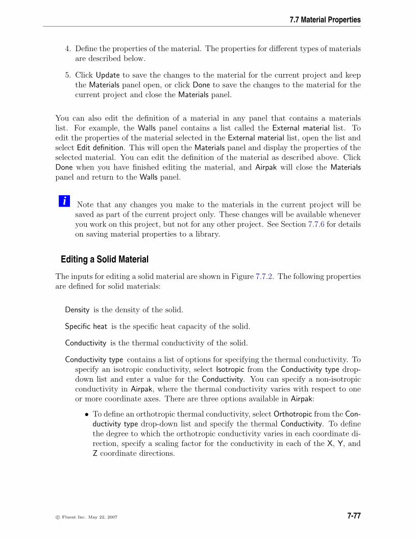
7.7 Material Properties
4. Define the properties of the material. The properties for different types of materialsare described below.
5. Click Update to save the changes to the material for the current project and keepthe Materials panel open, or click Done to save the changes to the material for thecurrent project and close the Materials panel.
You can also edit the definition of a material in any panel that contains a materialslist. For example, the Walls panel contains a list called the External material list. Toedit the properties of the material selected in the External material list, open the list andselect Edit definition. This will open the Materials panel and display the properties of theselected material. You can edit the definition of the material as described above. ClickDone when you have finished editing the material, and Airpak will close the Materialspanel and return to the Walls panel.
i Note that any changes you make to the materials in the current project will besaved as part of the current project only. These changes will be available wheneveryou work on this project, but not for any other project. See Section 7.7.6 for detailson saving material properties to a library.
Editing a Solid Material
The inputs for editing a solid material are shown in Figure 7.7.2. The following propertiesare defined for solid materials:
Density is the density of the solid.
Specific heat is the specific heat capacity of the solid.
Conductivity is the thermal conductivity of the solid.
Conductivity type contains a list of options for specifying the thermal conductivity. Tospecify an isotropic conductivity, select Isotropic from the Conductivity type drop-down list and enter a value for the Conductivity. You can specify a non-isotropicconductivity in Airpak, where the thermal conductivity varies with respect to oneor more coordinate axes. There are three options available in Airpak:
• To define an orthotropic thermal conductivity, select Orthotropic from the Con-ductivity type drop-down list and specify the thermal Conductivity. To definethe degree to which the orthotropic conductivity varies in each coordinate di-rection, specify a scaling factor for the conductivity in each of the X, Y, andZ coordinate directions.
c© Fluent Inc. May 22, 2007 7-77

Building a Model
• To specify an anisotropic thermal conductivity, specify the thermal Conductiv-ity and then select Anisotropic from the Conductivity type drop-down list. Todefine the degree to which the anisotropic conductivity varies in each direc-tion, specify a scaling factor for the conductivity in each of the XX, XY, XZ,YX, YY, YZ, ZX, ZY, and ZZ directions, respectively, next to Tensor. Alterna-tively, you can click on the Edit button to the right of the Tensor text entryfield. This opens the Anisotropic tensor panel (Figure 7.7.3).
Figure 7.7.3: The Anisotropic tensor Panel
Enter the scaling factors for the conductivity in the following way in theAnisotropic tensor panel:
XX XY XZ
YX YY YZ
ZX ZY ZZ
• To specify a biaxial thermal conductivity, select Biaxial from the Conductivitytype drop-down list and specify the thermal Conductivity. To define the degreeto which the biaxial conductivity varies in each direction, specify a scalingfactor for the conductivity in the Normal and In-plane directions.
The thermal conductivity is used when temperature is included in the problem (seeSection 6.4.2). When modeling a transient problem, density and specific heat will alsobe used. See Chapter 20 for details on transient simulations.
Editing a Fluid Material
The inputs for editing a fluid material are shown in Figure 7.7.4.
The following properties are defined for fluid materials:
Vol. expansion is the volumetric expansion coefficient of the fluid.
Viscosity is the fluid dynamic viscosity.
7-78 c© Fluent Inc. May 22, 2007

7.7 Material Properties
Figure 7.7.4: The Materials Panel for a Fluid Material
Density is the fluid density.
Specific heat is the specific heat capacity of the fluid.
Conductivity is the thermal conductivity of the fluid (which can be velocity- or temperature-dependent).
Diffusivity is the diffusivity of the fluid.
Molecular weight is the molecular weight of the fluid.
The density and viscosity of the fluid are used in all flow problems, but Airpak automat-ically sets an effective viscosity when the flow is turbulent, as described in Section 6.4.3.The thermal conductivity and specific heat are used when temperature is included in theproblem (see Section 6.4.2). Again, Airpak automatically sets an effective conductivitywhen the flow is turbulent. The volumetric expansion coefficient of the fluid is used whennatural convection due to gravity effects is present (see Section 6.4.4). If gravity is notactivated, the volumetric expansion coefficient is not used. By default, Airpak uses theBoussinesq approximation (see Section 31.3.1) to model the buoyancy force and in this
c© Fluent Inc. May 22, 2007 7-79

Building a Model
case Airpak uses a constant density in its calculations. If you select the ideal gas lawto model the buoyancy force, Airpak uses a density that varies as p
RT, as described in
Section 31.3.2.
i If you use the ideal gas law and you have created a new fluid material, make surethat you specify the correct molecular weight for the new material.
Editing a Surface Material
The inputs for editing a surface material are shown in Figure 7.7.5.
Figure 7.7.5: The Materials Panel for a Surface Material
The following properties are defined for surface materials:
Roughness is the roughness of the entire surface, where zero represents a perfectlysmooth surface.
Emissivity is the emissivity of the surface.
7-80 c© Fluent Inc. May 22, 2007

7.7 Material Properties
Solar absorptance - normal incidence is the fraction of direct solar irradiation energythat is absorbed by the semi-transparent surface for a direct solar irradiation beamnormal to the surface.
Solar transmittance - normal incidence is the fraction of direct solar irradiation energytha tpasses through the semi-transparent surface for a direct solar irradiation beamnormal to the surface.
Diffuse hemispherical absorptance is the fraction of diffuse solar irradiation energy thatis absorbed by the semi-transparent surface.
Diffuse hemispherical transmittance is the fraction of diffuse solar irradiation energythat passes through the semi-transparent surface.
The roughness of the surface is used when the flow is turbulent, as described in Sec-tion 6.4.3. The emissivity is used when radiation is modeled (see Chapter 22). Solar anddiffuse absorptance and transmittance properties are used when solar loading is modeled(see Section 22.5). Properties of semi-transparent surface radiation account for its solarperformance relative to direct solar irradiation and diffuse solar irradiation. One semi-transparent surface material may be used to represent the lumped effect of fenestrationcontaining several glazing layers. For any semi-transparent surface, the sum of absorp-tance, transmittance, and reflectance must equal 1.0 for each type of solar irradiation.Therefore, it is sufficient to specify only two of the three solar performance properties foreach type of radiation.
7.7.3 Viewing the Properties of a Material
You can view the properties of a material using any panel that contains a materials list.For example, the Walls panel contains a list called the External material list. To view theproperties of the material selected in the External material list, open the list and selectView definition.
The Message window will report the properties of the material, e.g., for the default ma-terial in the External material list in the Walls panel:
Material name: "Al-Polished Partition-surface", type surface
Roughness = 0.0 m
Emissivity = 0.041
7.7.4 Copying a Material
To copy a material, right-click on the material item in the Model manager window andselect Copy material in the pull-down menu. You can also copy a material by select-
ing the material item in the Model manager window and clicking on the but-ton. A new material will be created under the Model node (Figure 7.7.6) with the
c© Fluent Inc. May 22, 2007 7-81

Building a Model
name of the material that you have copied and the suffix .1. For example, if youmake a copy of the solid material Al-Pure, the new material will have the default nameAl-Pure.1. The properties of the new material are the same as the properties of the ma-terial that was copied. The properties of the new material can be edited as described inSection 7.7.2.
Figure 7.7.6: The Materials Node Under the Model Node
i Note that any changes you make to the materials in the current project will besaved as part of the current project only. These changes will be available wheneveryou work on this project, but not for any other project. See Section 7.7.6 for detailson saving material properties to a library.
7.7.5 Creating a New Material
To create a new material, click on the button in the Object creation toolbar. A newmaterial will be created with the default name material.n, where n is the next sequentialnumber among numbered materials. The name of the new material will appear underthe Model node in the Model manager window (Figure 7.7.6) and in the Name text entrybox in the Materials panel. See Section 7.7.2 for details on renaming a material.
You can also create a new material in any panel that contains a materials list. Forexample, the Walls panel contains a list called the External material list. To create a newmaterial, open the External material list and select Create material. This will open theMaterials panel and create a material called wall.1 ext material in this example. Youcan rename and edit the material using the Materials panel. Click Done when you havefinished editing the material, and Airpak will close the Materials panel and return to theWalls panel.
i Note that any changes you make to the materials in the current project will besaved as part of the current project only. These changes will be available wheneveryou work on this project, but not for any other project. See Section 7.7.6 for detailson saving material properties to a library.
7-82 c© Fluent Inc. May 22, 2007

7.7 Material Properties
7.7.6 Saving Materials and Properties
By default, Airpak searches for the materials file that is provided with the standard Airpakdistribution. This file includes a large collection of material definitions that are availableto all Airpak users. It is located in the AIRPAK ROOT/airpak lib directory and is calledthe materials file. Different materials files can be accessed using different libraries. Ifyou wish to modify the properties of materials that are included with Airpak, there aretwo ways to do this:
• create a new library and copy materials to the library
• copy materials from the main library into the model
You can access as many different materials files as you like. Note that all the materials filesmust have the same name (materials), and so must be located in different directories.
When you use the Model manager window or the Materials panel to create, modify, ordelete an existing material, these modifications are saved as part of the current projectonly. These changes will be available whenever you work on this project, but not for anyother project.
To create a new library of materials, you have two options:
• Create your own local materials file using the following procedure:
1. Select Create material library in the Model menu.
Model−→Create material library
2. Select all the materials that you want to save from the list in the Selectionpanel (Figure 7.7.7). Click All if you want to select all the materials in thelist. Click None to deselect all of the materials in the list.
3. Click Done when you have finished selecting the materials to be saved. Thiswill open the File selection dialog box, in which you can specify the filename(materials) and directory to which the materials file is to be saved. SeeSection 2.1.8 for details about the file selection dialog box.
To use the new materials file, add the path for the materials file to the list oflibrary paths in the Library path panel so that the new and edited materials can bemade available for all your Airpak projects. See Section 6.3.5 for details.
This allows you to create new materials or edit previously defined materials usingthe Materials panel. If a material is defined in the global materials file and also ina user-defined file, Airpak will take the definition of the material from the first filethat it loads and will ignore any subsequent redefinitions of the material. The orderin which the files are loaded is the same as the order in which they are specified inthe Library path panel (see Section 6.3.5).
c© Fluent Inc. May 22, 2007 7-83

Building a Model
Figure 7.7.7: The Selection Panel for Saving Materials
• Create a new library using the Library path panel as described in Section 6.3.5.
Once you have created a new library, the name of the library will appear underthe Libraries node in the Model manager window. To add new or previously-definedmaterials to a new library, select the material item and drag it into the new librarynode. This will create a new materials file. If you drag any new materials into thesame library, the materials file will be appended with the new materials.
7.7.7 Deleting a Material
If there are materials in your local materials library that you no longer need, you caneasily delete them. Select the material under the Materials (or Model) node and click on
the button in the Object modification toolbar or click Delete in the Materials panel(e.g., Figure 7.7.2). The selected material will be removed from your model.
7.7.8 Defining Properties Using Velocity-Dependent Functions
You can define the thermal conductivity of a fluid in Airpak to be a function of velocity.The thermal conductivity of a fluid can be defined using a power law form:
k = Bvn (7.7-1)
7-84 c© Fluent Inc. May 22, 2007

7.7 Material Properties
where k is the thermal conductivity of the fluid, v is the velocity, and B and n areconstants.
To define the thermal conductivity of the fluid as velocity-dependent, enable the checkbox next to Conductivity and click the adjacent Edit button for a fluid material in theMaterials panel. This will open the Temperature or velocity dependent fluid conductivitypanel. Select Velocity at the top of the panel (Figure 7.7.8).
Figure 7.7.8: The Temperature or velocity dependent fluid conductivity PanelShowing the Velocity-Dependent Inputs
Specify the Coefficient (B in Equation 7.7-1) and the Exponent (n in Equation 7.7-1) andclick Accept to define the velocity-dependent thermal conductivity of the fluid.
i You must specify these inputs in SI units.
7.7.9 Defining Properties Using Temperature-Dependent Functions
Many material properties in Airpak can be defined as functions of temperature. Formost properties, you can define a constant, linear, or piecewise-continuous function oftemperature. To define a property as temperature-dependent, enable the check box nextto the property and click the adjacent Edit button in the Materials panel. This willopen the Temperature dependent parameter panel. Figure 7.7.9 shows an example of atemperature-dependent parameter panel (the Temperature dependent solid specific heatpanel).
Note that if you are defining a temperature-dependent thermal conductivity for a fluid,you will need to select the Temperature option at the top of the Temperature or velocitydependent fluid conductivity panel.
There are three options for specifying the temperature dependence of a parameter:
c© Fluent Inc. May 22, 2007 7-85
Building a Model
Figure 7.7.9: Example of a Temperature dependent Parameter Panel
Constant allows you to define the property as a constant.
Linear allows you to define the property in terms of a linear equation:
v = v0 + C(T − Tref) (7.7-2)
where v0 (v0) is a reference value, C (C) is a constant, and Tref (Tref) is the referencetemperature.
Curve allows you to define the property as a curve consisting of piecewise-continuousline segments. Airpak allows you to describe the curve either by positioning a seriesof points on a graph using the Temperature/value curve window or by specifying alist of temperature/value coordinate pairs using the Curve specification panel. Theseoptions are described below.
Using the Temperature/value curve Window
You can specify a piecewise linear variation of a property with temperature using theTemperature/value curve graphics display and control window (Figure 7.7.10). To openthe Temperature/value curve window, select Curve in the Temperature dependent parameterpanel (Figure 7.7.9) and click on Edit. Select Graph editor from the resulting list.
The following functions are available for creating, editing, and viewing a curve:
• To create a new point on the curve, click on the curve with the middle mousebutton.
• To move a point on the curve, hold down the middle mouse button while positionedover the point, and move the mouse to the new location of the point.
7-86 c© Fluent Inc. May 22, 2007

7.7 Material Properties
Figure 7.7.10: The Temperature/value curve Graphics Display and ControlWindow
c© Fluent Inc. May 22, 2007 7-87

Building a Model
• To delete a point on the curve, click the right mouse button on the point.
• To zoom into an area of the curve, position the mouse pointer at a corner of thearea to be zoomed, hold down the left mouse button and drag open a selectionbox to the desired size, and then release the mouse button. The selected area willthen fill the Temperature/value curve window, with appropriate changes to the axes.After you have zoomed into an area of the model, click on Full range to restore thegraph to its original axes and scale.
• To set the minimum and maximum values for the scales on the axes, click on Setrange. This will open the Set range panel (Figure 7.7.11).
Figure 7.7.11: The Set range Panel
Enter values for Min X, Min Y, Max X, and Max Y and click Accept.
• To load a previously defined curve, click on Load. This will open the Load curvefile selection dialog box. Select the file containing the curve data and click Accept.See Section 2.1.8 for details on selecting a file.
• To save a curve, click on Save. This will open the Save curve dialog box, in whichyou can specify the filename and directory to which the curve data is to be saved.
You can use the Print button to print the curve. See Section 3.5 for details on savinghardcopy files.
Click Done when you have finished creating the curve; this will store the curve and closethe Temperature/value curve graphics display and control window. Once the curve isdefined, you can view the pairs of coordinates defining the curve in the Curve specificationpanel (see Figure 7.7.12 for the pairs of coordinates for the curve shown in Figure 7.7.10).
Using the Curve specification Panel
You can define a piecewise linear variation of a property with temperature using theCurve specification panel (Figure 7.7.12). To open the Curve specification panel, selectCurve in the Temperature dependent parameter panel (Figure 7.7.9) and click on Edit.Select Text editor from the resulting list.
7-88 c© Fluent Inc. May 22, 2007

7.7 Material Properties
Figure 7.7.12: The Curve specification Panel
To define a curve, specify a list of coordinate pairs in the Curve specification panel.It is important to give the numbers in pairs, but the spacing between numbers is notimportant. Click Accept when you have finished entering the pairs of coordinates; thiswill store the values and close the Curve specification panel.
Once the pairs of coordinates have been entered, you can view the curve in the Temper-ature/value curve graphics display and control window. See Figure 7.7.10 for the curvefor the values shown in Figure 7.7.12.
c© Fluent Inc. May 22, 2007 7-89

Building a Model
7.8 Custom Assemblies
In HVAC models, it is not uncommon to encounter cases where a given combination ofmodeling objects appears in more than one model. It may be necessary, for example, tomodel the use of a standard diffuser in conjunction with several different types of roomsand/or other indoor equipment. Airpak allows you to create the standard assembly once,and then use it in other models.
Assemblies are collections of Airpak objects (e.g., vents, fans, blocks) that have beendefined together as a group (see Section 7.6 for information on grouping objects) andstored as a single unit.
7.8.1 Creating and Adding an Assembly
You can create an assembly to be used in your Airpak model using one of the followingmethods:
• Create a group containing all the objects that you want to be in the assembly andthen create the assembly from the group. See Section 7.6 for details on creatinggroups.
• Create an assembly first and then add individual objects or groups to the assembly.
Creating an Assembly From a Group of Objects
To create an assembly from an existing group of objects, select Create assembly in theEdit−→Current group menu. The objects in the group will be added as items under thenew assembly node in the Model manager window (Figure 7.8.1).
Figure 7.8.1: An Assembly Node in the Model manager Window
Alternatively, you can create a new assembly by right-clicking on the group item underthe Groups node in the Model manager window and selecting Create assembly in the pull-down menu.
7-90 c© Fluent Inc. May 22, 2007
7.8 Custom Assemblies
Creating an Assembly Item Without Using a Group of Objects
To create an empty assembly item under the Model node in the Model manager window
(Figure 7.8.1), click on the button in the Object creation toolbar. If the Assembliespanel is already open, you can also click on New in the Assemblies panel to create a newassembly.
Alternatively, you can use the <Control> and <Shift> keys in combination with themouse to select multiple objects in the Model manager window (see Section 2.2.2). Tocreate an assembly from the selected items, right-click on one of the items and selectCreate assembly in the pull-down menu.
Adding Objects to an Assembly
To add objects to an existing assembly, use one of the following methods:
• Select one or more object items in the Model manager window and drag them intothe desired assembly node.
• Select one or more objects in the graphics window by holding down the <Shift> keyand dragging open a selection box around the objects with the left mouse button. Inthe Model manager window, drag the highlighted item(s) into the desired assemblynode.
• Right-click on the assembly item in the Model manager window and select Createin the first pull-down menu. In the subsequent pull-down menu, select the type ofobject you wish to add to the assembly. See Chapters 8–19 for information aboutthe different objects in Airpak.
7.8.2 Editing Properties of an Assembly
To edit properties of an assembly item, use the following procedure:
1. Click on the button in the Object modification toolbar or right-click on theassembly item in the Model manager window and select Edit object in the pull-downmenu. This will open the Assemblies panel (Figures 7.8.2 and 7.8.3).
2. Change the description of the assembly, if required, in the Info tab of the Assem-blies panel. Changing the description of an assembly is the same as changing thedescription of an object. See Section 7.4.1 for details.
3. Change the graphical style of the assembly, if required. Changing the graphicalstyle of an assembly is the same as changing the graphical style of an object. SeeSection 7.4.2 for details.
c© Fluent Inc. May 22, 2007 7-91

Building a Model
Figure 7.8.2: The Assemblies Panel (Definition Tab)
4. In the Definition tab, select the assembly to be added to the model (Figure 7.8.2).There are two options:
External Assembly allows you to use an assembly that was created in a previousAirpak session. Specify the name of the project where the assembly was createdin the Project definition text entry field. You can enter your own filename,which can be a full pathname to the file (beginning with a / character ona UNIX system or a drive letter on Windows) or a pathname relative tothe directory in which Airpak was started. Alternatively, you can choose afilename by clicking on the square button located next to the Project definitiontext field and then selecting the file in the resulting File selection dialog box.See Section 2.1.8 for more information on the File selection dialog box.
i When you use the external assembly option to define your assembly, theassembly is not copied into your model. Airpak creates a link to the projectthat contains the assembly. To copy the assembly into the model and storeit in the model, you should create the link to the external assembly usingthe External Assembly option as described above, then select the InternalAssembly option and click Update. If the external assembly is not copied
7-92 c© Fluent Inc. May 22, 2007
7.8 Custom Assemblies
into the current model, all modifications made to the external assemblywill be lost.
Internal Assembly allows you to specify a group that is defined in the currentmodel to be used as an assembly. This option is selected by default. Tospecify a group, click the Define using group button and choose a group fromthe list in the subsequent Selection panel.
5. (optional) To translate the assembly by a specified distance from its original posi-tion, define the distance of the translation from the original position by specifyingan offset in each of the coordinate directions: X offset, Y offset, and Z offset.
Note that if you want to perform a transformation that is different from that pro-vided by the Assemblies panel, you can create an initial assembly and then performadditional transformations using the Move assembly panel. The Move assembly panelis identical to the Move all objects in model panel described in Sections 7.2.1 and7.2.2. You should also note the extra details for moving an object in Section 7.3.7.
i If you scale, rotate, mirror, or translate the assembly, these operations willbe performed with respect to the assembly’s local coordinate system and notthe global coordinate system.
6. In the Meshing tab, specify whether you want to have the assembly meshed sepa-rately from the rest of your Airpak model (Figure 7.8.3).
(a) To allow Airpak to generate a non-conformal mesh, turn on the Mesh separatelyoption. See Chapter 26 for details about generating a mesh.
(b) If you selected Mesh separately, specify the Slack distance around the boundingbox of the assembly (Min X, Max X, Min Y, Max Y, Min Z, Max Z). Thebounding box will be moved outward by the amount of slack that is specified.Additionally, each of the slack distances can be assigned by aligning the edgesof the assembly bounding box to existing edges of objects or other assemblies.To do so, follow the procedure described in Section 7.3.8.
For example, to set the slack distance in the Min X direction, you would firstclick Min X displayed in orange in the Meshing tab of the Assemblies panel,then click the edge of the object in the graphics window that you want to alignwith the Min X edge of the assembly bounding box.
(c) If you selected Mesh separately, you can specify the Minimum gap that separatesobjects in the assembly in the X, Y, and Z directions. This specification is usedby Airpak whenever the distance between two objects inside the assemblyis less than this value, but greater than the model’s zero tolerance. If youdon’t specify the Minimum gap (i.e., the specified values are equal to 0), theseparation values will be inherited from the global mesh settings.
c© Fluent Inc. May 22, 2007 7-93

Building a Model
Figure 7.8.3: The Assemblies Panel (Meshing Tab)
(d) If you selected Mesh separately, you can specify the Mesh type for the objectsin the assembly. Assemblies meshed separately can have a mesh type differentfrom the type used to mesh the outside room.
For example, if the global mesh type has been specified as Hexa unstructuredin the Mesh control panel, a Tetra mesh type can be used to mesh the objectsinside the assembly. By default, Airpak uses the same mesh type specified inthe Mesh control panel to mesh the objects inside the assembly.
(e) If you selected Mesh separately, you can specify a limit on the element size ofthe assembly mesh in the x, y, and z coordinate directions. To do so, selectMax X, Max Y, and Max Z size specifications and set each one to the desiredmaximum element length in each direction. If no values are specified, Airpakuses the global values specified in the Mesh control panel.
7. Specify whether you want to fix the values for the units in the panel. See Sec-tion 5.4.2 for details.
7-94 c© Fluent Inc. May 22, 2007

7.8 Custom Assemblies
8. Click Update to position the assembly according to the specifications in the Assem-blies panel. Click Done to position the assembly and close the Assemblies panel.
c© Fluent Inc. May 22, 2007 7-95

Building a Model
7.8.3 Assembly Viewing Options
There are several ways to view an assembly in your Airpak model. Expanding the assem-bly node in the Model manager window will display the objects in the assembly as theywould normally look. Closing the assembly node will display only the bounding box ofthe assembly.
In a more complicated model, you can choose to view only one particular assembly whilehiding the rest of your Airpak model. To change the display in this manner, right-clickon the desired assembly node under the Model node in the Model manager window andturn on the View separately option in the pull-down menu. The assembly node will betemporarily moved up one level in the tree and the Model node will be closed, whichresults in only the assembly being displayed. To return to the default display settings,right-click on the assembly node and turn off the View separately option.
7.8.4 Selecting an Assembly
There are two ways to select an assembly:
• Select the name of assembly under the Model node in the Model manager windowusing the left mouse button.
• Position the mouse cursor over the assembly in the graphics window, hold downthe <Shift> key on the keyboard, and click the left mouse button.
7.8.5 Editing Objects in an Assembly
Once you have created an assembly or read an assembly into your Airpak model, youcan edit the individual objects in the assembly. To edit an object, select the object item
under the assembly node and click on the button in the Object modification toolbaror select Edit in the Edit−→Current object menu. This will open the Object panel, whereyou can edit any of the properties of any individual object.
Alternatively, you can edit an assembly by right-clicking on the assembly item in theModel manager window and selecting Edit object in the pull-down menu.
7.8.6 Copying an Assembly
To copy an assembly in your model, select the assembly and click on the button inthe Object modification toolbar or select Copy in the Edit−→Current object menu. Thiswill open the Copy assembly panel. The procedure for copying an assembly is the sameas copying an object using the Copy object panel, as described in Section 7.3.9.
Alternatively, you can copy an assembly by right-clicking on the assembly item in theModel manager window and selecting Copy object in the pull-down menu.
7-96 c© Fluent Inc. May 22, 2007

7.8 Custom Assemblies
i If you scale, rotate, mirror, or translate the assembly, these operations will beperformed with respect to the assembly’s local coordinate system and not the globalcoordinate system.
7.8.7 Moving an Assembly
To move an assembly, select the assembly and click on the button in the Objectmodification toolbar or select Move in the Edit−→Current object menu. This opens theMove assembly panel. You can apply various transformations to the assembly. Theoperations in the Move assembly panel are the same as those in the Move all objects inmodel panel (Figure 7.2.6). The Scale option is described in Section 7.2.1, and the Rotate,Mirror, and Translate options are described in Sections 7.2.2 and 7.3.7.
Alternatively, you can move an assembly by right-clicking on the assembly item in theModel manager window and selecting Move object in the pull-down menu.
i If you scale, rotate, mirror, or translate the assembly, these operations will beperformed with respect to the assembly’s local coordinate system and not the globalcoordinate system.
7.8.8 Saving an Assembly
To save an assembly to be used in another model, click Write assembly in the Assembliespanel (Figure 7.8.2). This will open the Save project panel. See Section 3.4 for informationon the Save project panel. You can save the project containing the assembly to anydirectory, but it is recommended that you create a local assemblies directory where youcan save all the assemblies you create.
Alternatively, you can save an assembly as a separate project by right-clicking on theassembly item in the Model manager window and selecting Save as project in the pull-downmenu. See Section 3.4 for details about saving projects.
7.8.9 Loading an Assembly
To load an assembly that was created in another model, right-click on the assembly itemin the Model manager window and select Load assembly in the pull-down menu. This willopen the Load project panel, which is similar to the Open project panel. See Section 6.2for information on the Open project panel.
7.8.10 Merging an Assembly With Another Project
To merge an assembly with another project, right-click on the assembly item in theModel manager window and select Merge project in the pull-down menu. This will openthe Merge project panel. See Section 3.3 for information about using this panel.
c© Fluent Inc. May 22, 2007 7-97

Building a Model
7.8.11 Deleting an Assembly
To delete an assembly, select the assembly and click on the button in the Objectmodification toolbar, select Delete in the Edit−→Current object menu, or click Delete inthe Assemblies panel (Figure 7.8.2). The selected assembly will be removed from themodel and from the Model manager window.
Alternatively, you can delete an assembly by right-clicking on the assembly item in theModel manager window and selecting Delete in the pull-down menu.
To recover a deleted assembly, you can undo the delete operation by selecting the Undooption in the Edit menu. See Section 2.1.2 for more details on using undo and redooperations.
7.8.12 Expanding an Assembly Into Its Components
Once you have created an assembly or read an assembly into your Airpak model, youcan expand the assembly into its individual components. To expand an assembly, simplyexpand the assembly node in the Model manager window. The assembly will be expandedinto its individual components that can be edited separately.
Alternatively, you can expand an assembly into its components by right-clicking on theassembly item in the Model manager window and selecting Open subtree in the pull-downmenu. To view the assembly as a single object, you can close the node or select Closesubtree in the pull-down menu.
7.8.13 Summary Information for an Assembly
To view a brief summary of the contents of an assembly, right-click the assembly item inthe Model manager window and select Summary information in the pull-down menu. Thiswill open the Assembly contents panel, as shown in Figure 7.8.4. This panel lists the totalnumber of objects in the assembly along with the number of objects of each individualobject-type.
Figure 7.8.4: The Assembly contents Panel
7-98 c© Fluent Inc. May 22, 2007

7.9 Checking the Design of Your Model
7.8.14 Total Volume of an Assembly
To display the total volume occupied by all the objects in an assembly, right-click theassembly item in the Model manager window and select Total volume in the pull-downmenu. The total volume will be displayed in the Message window.
7.8.15 Total Area of an Assembly
To display the total area occupied by all the objects in an assembly, right-click theassembly item in the Model manager window and select Total area in the pull-down menu.The total area will be displayed in the Message window.
7.9 Checking the Design of Your Model
Airpak provides two ways to check your model for design problems: object and materialsummaries, and design checks. Object and material summaries, and design checks aredescribed in detail below.
7.9.1 Object and Material Summaries
Object and material summaries provide an on-screen catalog of all objects in the model,(including names, descriptions, dimensions, locations, and all physical and thermal prop-erties associated with each object) and any materials you have created or edited. Thesummary allows you to review the contents of your model as a means of examining thedesign. To create an object and material summary, select Summary (HTML) in the Viewmenu. The HTML version of the summary will be displayed in your web browser. Air-pak will automatically launch your web browser (Netscape, IE, or Mozilla), as shown in(Figure 7.9.1).
View−→Summary (HTML)
The summary displays a list of all the objects in the model and all the parameters thathave been set for each object. The information is grouped by object types (e.g., blocks,fans, vents). For each object type, the number of objects of that type is indicated,along with the Name and Shape of every object. If specified, other information will belisted, such as Material, Power, Radiation, Loss specification, etc. If certain properties (e.g.,radiation) are specified, you can view the detailed version of the summary by clicking theappropriate object names or property specifications. For example, if you click block.3 inthe summary shown in Figure 7.9.1, the detailed version of the summary will be displayedas shown in Figure 7.9.2.
7.9.2 Design Checks
Design checks test the model for problems in the design. To perform an automated designcheck, select Check model in the Model menu.
c© Fluent Inc. May 22, 2007 7-99

Building a Model
Figure 7.9.1: Model Summary
7-100 c© Fluent Inc. May 22, 2007

7.9 Checking the Design of Your Model
Figure 7.9.2: Detailed Summary
c© Fluent Inc. May 22, 2007 7-101

Building a Model
Model−→Check model
In the design check, Airpak searches for incidences of overlapping objects, violations ofphysics (e.g., openings not associated with walls), and unacceptable data (e.g., valuesout of range for individual specifications).
The results of the design check are reported sequentially in the Airpak Message window.Informative messages appear as blue text, while flaws or design errors detected by thecheck appear as red text. Airpak highlights the overlapping sections of all intersectingobjects in red in the graphics window. To restore the model colors to their defaults,select Check model again.
If Airpak detects a large number of flaws in the model, the on-screen report may exceedthe size of the Message window. To review the entire list of flaws, you can either expandthe Message window, or print the contents of the Message window to a file using the Logoption in the Message window (see Section 2.1.6).
Note that the design check is performed automatically when you generate a mesh for themodel.
7-102 c© Fluent Inc. May 22, 2007

Chapter 8. Blocks
A block is a three-dimensional modeling object. Block geometries include prism (rectan-gular box), cylinder, 3D polygon, ellipsoid, elliptical cylinder and 3D CAD. Block typesinclude solid, hollow, and fluid.
Physical, species, and thermal characteristics that need to be specified vary accordingto the block type. All types of blocks (or individual sides of the blocks) can exchangeradiation with other objects in the model. Blocks exist within the room, so any partof their non-contact surfaces may be exposed to the fluid in the room. By default, theno-slip condition for fluid velocity applies at all block surfaces. For turbulent flows, youcan specify a roughness parameter.
To configure a solid, hollow, or fluid block in your model, you must specify its geom-etry (including location and dimensions) and type, as well as its physical and thermalcharacteristics.
In this chapter, information about the characteristics of a block is presented in thefollowing sections:
• Section 8.1: Geometry, Location, and Dimensions
• Section 8.2: Block Type
• Section 8.3: Surface Roughness
• Section 8.4: Physical and Thermal Specifications
• Section 8.5: Block-Combination Thermal Characteristics
• Section 8.6: Adding a Block to Your Airpak Model
8.1 Geometry, Location, and Dimensions
Block location and dimension parameters vary according to block geometry. Block ge-ometries include prism, cylinder, 3D polygon, ellipsoid, elliptical cylinder, and 3D CAD.These geometries are described in Section 7.4.4. Note that network blocks can only haveprism geometries.
c© Fluent Inc. May 22, 2007 8-1

Blocks
8.2 Block Type
There are three types of Airpak blocks: solid, hollow, and fluid. Although they sharecertain specifications, each is unique in purpose and characteristics:
• Solid blocks represent actual solid objects and can possess physical and thermalcharacteristics such as density, specific heat, thermal conductivity, and total heatflux. Airpak considers the interior of a solid block to be part of the computationaldomain and includes the block internal temperature distribution as part of themodel solution.
• Hollow blocks represent three-dimensional regions of the model for which only sidecharacteristics are important. Airpak does not mesh or solve for temperature orflow within regions bounded by the sides of a hollow block. Hollow-block surfacescan be specified as adiabatic (impervious to heat flow) or as possessing a fixed,uniform temperature or heat flux.
• Fluid blocks are regions of the model where fluid properties can be specified in-dependently of those specified for the Default fluid in the Basic parameters panel(see Section 6.4.7). Individual side parameters for fluid blocks are specified in thesame manner as those for solid and hollow blocks. If individual side parameters arespecified on a side of a fluid block, a zero thickness wall is defined for that side ofthe block.
8.3 Surface Roughness
In fluid dynamics calculations, it is common practice to assume that boundary surfacesare perfectly smooth. In laminar flow, this assumption is valid, because the length scalesof typical rough surfaces are much smaller than the length scales of the flow. In turbulentflow, however, the length scales of the flow eddies are much smaller than laminar lengthscales; therefore, it is sometimes necessary to account for surface roughness. Surfaceroughness acts to increase resistance to flow, leading to higher rates of heat transfer.
Airpak assumes, by default, that all surfaces of a block are hydrodynamically smooth, andapplies standard no-slip boundary conditions. For turbulent-flow simulations in whichroughness is significant, however, you can specify a roughness factor for the entire blockor (for solid, hollow, and fluid blocks) each individual side of the block. The roughnessfactor is defined as part of the properties of the surface material specified for the block.The purpose of the roughness factor is to approximate the average height of the surfacetexture on the block.
8.4 Physical and Thermal Specifications
Block physical and thermal specifications vary according to block type:
8-2 c© Fluent Inc. May 22, 2007

8.5 Block-Combination Thermal Characteristics
• Solid block specifications include parameters related to material properties.
• Hollow block specifications, on the other hand, include only parameters related tothe block surface itself, such as temperature, heat flux, species, and whether or notthe surface is adiabatic.
• Fluid block specifications relate to the properties of the fluid within the block.
In addition to specifying parameters for the entire block, Airpak allows you to specifyparameters for each individual side of the block. Side-specific parameters include thoserelated to surface thermal characteristics (e.g., temperature and heat flux) as well asradiation.
If you specify the side of a block as adiabatic, Airpak treats it as impervious to heat flowin the direction normal to its surface. When a block side is specified as fixed temperature,Airpak assigns a constant temperature to the side. If you specify a block side as fixedheat, Airpak assumes that it emits or absorbs heat uniformly at a constant rate. You canspecify a fixed heat flux in terms of either total heat flux or heat flux per unit area. Ifthe side of the block is subject to solar loading, you can calculate the solar radiation fluxusing the solar flux macro (described in Section 22.5) and then use the value of the solarradiation flux as the specified heat flux for the side of the block.
8.5 Block-Combination Thermal Characteristics
Blocks can be combined with other blocks and objects to achieve a wide variety ofcomplex shapes. In combining blocks to create custom objects, special care must betaken to ensure that the assignment of thermal characteristics achieves the intendedrepresentation of the object being modeled. The following examples illustrate the generalrules that govern heat transfer in objects created by combining two or more objects.
8.5.1 Blocks with Coincident Surfaces
When a model involves two blocks with coincident surfaces (see Figure 8.5.1), Airpakemploys two basic rules to govern the thermal characteristics in the region of contact:
• If both blocks are specified as conducting solid blocks, Airpak computes the amountof heat transferred between the blocks. To apply a thermal resistance between theblocks at the contact surface (representing, for example, a coating layer between theblocks), locate and specify a partition at the region of coincidence (see Chapter 14).
• When one (or both) of the blocks is specified as hollow, no heat transfer occursacross the coincident surface. Figure 8.5.2 shows an example configuration whereBlock A is a non-conducting, solid block and Block B is a hollow block with aspecified constant heat flux. Block A insulates the coincident region with respect
c© Fluent Inc. May 22, 2007 8-3

Blocks
Figure 8.5.1: Blocks with Coincident Surfaces
to heat flow, so heat is transferred away from Block B only on those surfaces exposedto the fluid in the room.
8.5.2 Blocks with Intersecting Volumes
Blocks with intersecting volumes follow rules similar to those outlined above for blockswith coincident surfaces. Intersecting blocks, such as those shown in Figure 8.5.3, how-ever, differ from blocks with coincident surfaces in that the characteristics of the inter-secting region are those of the last block created.
Consider, for example, a block configuration such as that shown in Figure 8.5.4, whereBlock B is created after Block A. The intersecting region (shaded) possesses the charac-teristics and parameters of Block B, regardless of which block is solid, hollow, or fluid intype, because Block B was the last block created.
If Block A is specified as a conducting solid block with a specified heat flux and BlockB is a hollow block, Airpak distributes the entire specified heat flux for Block A onlyin its non-intersecting volume. If, on the other hand, Block A is hollow and Block Bis a conducting solid block with a specified heat flux, Airpak distributes the power forBlock B throughout its entire volume, including the coincident region. If both blocks areconducting solid blocks, Airpak distributes specified heat flux and calculates temperaturedistributions throughout the entire volumes of both blocks, using the thermal propertiesof Block B in the coincident region.
8-4 c© Fluent Inc. May 22, 2007

8.5 Block-Combination Thermal Characteristics
Figure 8.5.2: Heat Flux for Blocks with Coincident Surfaces
Figure 8.5.3: Blocks with Intersecting Volumes
c© Fluent Inc. May 22, 2007 8-5

Blocks
Figure 8.5.4: Intersecting-Volume Properties
A Block and a Partition with Coincident Surfaces
When a block is positioned on a partition (see Figure 8.5.5), two rules govern the mannerin which the thermal characteristics of the partition affect those of the block:
Figure 8.5.5: Block Positioned on a Partition
• If the block is a conducting solid block and the partition has a non-zero thickness,the partition can be considered as a conducting solid block, and the rules govern-ing blocks with coincident surfaces apply. If the partition is specified with zerothickness, there is no heat transfer from the block to the partition.
• If the block is specified as fixed heat or fixed temperature, it can transfer heat tothe partition but cannot receive heat from the partition.
8-6 c© Fluent Inc. May 22, 2007

8.5 Block-Combination Thermal Characteristics
8.5.3 A Block and an Intersecting Partition
Blocks and partitions can be combined in a number of ways to produce complex objects.For example, a partition can be embedded in a block to introduce anisotropic conduc-tivity. When a block and a partition intersect (see Figure 8.5.6) two rules govern themanner in which the thermal characteristics of the partition affect those of the block:
Figure 8.5.6: Partition Intersecting a Block
• The thermal characteristics of a partition intersecting a conducting solid blockoverride those of the block, regardless of which object is created first. A partitionwith zero conductivity, for example, acts as an insulator within the block.
• If the block is specified as adiabatic, fixed heat, or fixed temperature, the presenceof the partition has no effect (i.e., the portion of the partition within the block isignored).
8.5.4 Blocks Positioned on an External Wall
When a block is located on an external wall (see Figure 8.5.7), the thermal interactionbetween the wall and block is governed by the following rules:
Figure 8.5.7: Block on an External Wall
c© Fluent Inc. May 22, 2007 8-7

Blocks
• A conducting solid block on an external wall exchanges heat with the wall. If theblock is specified as dissipating power, the side coincident with the wall transfersits heat to the wall.
• If a block in contact with a wall is specified as adiabatic, there is no heat transferbetween the block and the wall. If the block is specifid as fixed heat or fixedtemperature, it can transfer heat to the wall but cannot receive heat transferredfrom the wall.
8.5.5 Cylinder, Polygon, Ellipsoid, or Elliptical Cylinder Blocks Positioned on aPrism Block
When a prism block is in surface contact with a cylinder, polygon, ellipsoid, or ellipticalcylinder block (see Figure 8.5.8), the rules outlined above governing blocks with coincidentsurfaces apply:
Figure 8.5.8: Multiple Blocks in Contact
• If both blocks with coincident surfaces are designated as conducting solid blocks,Airpak calculates the amount of heat transferred between the blocks.
• If one (or both) blocks is non-conducting, no heat transfer occurs between theblocks, and Airpak computes heat transfer only from those surfaces exposed to theenclosure fluid as specified for each block. In Figure 8.5.8, for example, if BlockA is a nonconducting solid block and Blocks B and C are conducting blocks, heatis not allowed to flow from Block B to Block C (or vice versa) through Block A.Furthermore, the entire heat flux (if any) specified for Blocks B and C is transferredto the fluid through the non-coincident surfaces.
8-8 c© Fluent Inc. May 22, 2007

8.6 Adding a Block to Your Airpak Model
8.6 Adding a Block to Your Airpak Model
To include a block in your Airpak model, click on the button in the Object creation
toolbar and then click on the button to open the Blocks panel, shown in Figures 8.6.1and 8.6.2.
Figure 8.6.1: The Blocks Panel (Geometry Tab)
The procedure for adding a block to your Airpak model is as follows:
1. Create a block. See Section 7.3.2 for details on creating a new object and Sec-tion 7.3.9 for details on copying an existing object.
2. Change the description of the block, if required. See Section 7.4.1 for details.
3. Change the graphical style of the block, if required. See Section 7.4.2 for details.
4. In the Geometry tab, specify the geometry, position, and size of the block. Thereare five different kinds of geometry available for blocks in the Shape drop-down list.The inputs for these geometries are described in Section 7.4.4. See Section 7.3.6for details on resizing an object and Section 7.3.7 for details on repositioning anobject.
5. In the Properties tab, specify the type of the block by selecting Solid, Hollow, orFluid next to Block type. The lower part of the panel will change depending on yourselection of Block type.
c© Fluent Inc. May 22, 2007 8-9

Blocks
Figure 8.6.2: The Blocks Panel (Properties Tab)
6. Define the Surface specification for a block of the selected type. The options forsurface specification are described below.
7. Define the Thermal specification (or Fluid specification) for a block of the selectedtype. The options for thermal (or fluid) specification are described in Section 8.6.2.
8. (hollow blocks only) Specify the concentration of species at the surface of the block,if required. You can input the concentrations of the species at the surface of theblock using the Species concentration panel. To open this panel, select Species inthe Blocks panel and click Edit. See Chapter 21 for details on modeling speciestransport.
8.6.1 User Inputs for the Block Surface Specification
Define the Surface specification for a solid, hollow, or network block. The Surface specifi-cation can optionally be included for a fluid block also. The surface specification allowsyou to specify thermal and physical surface properties for the block. The user inputs forthe surface specification are shown below.
8-10 c© Fluent Inc. May 22, 2007
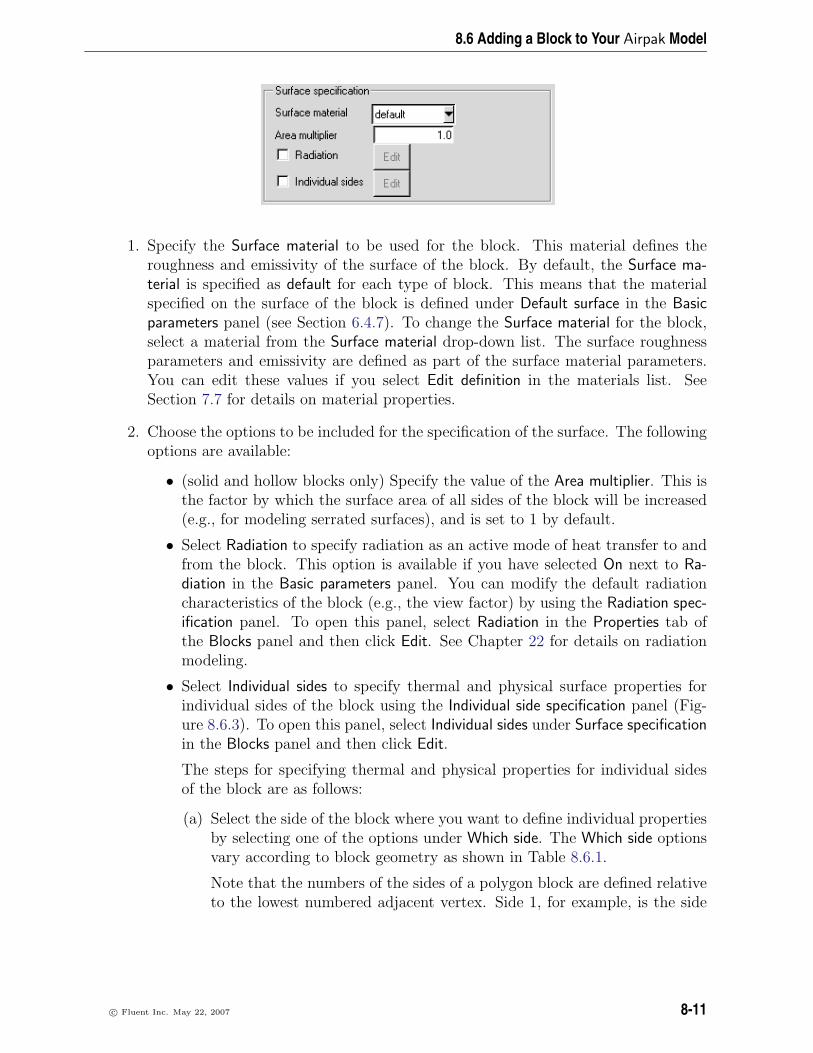
8.6 Adding a Block to Your Airpak Model
1. Specify the Surface material to be used for the block. This material defines theroughness and emissivity of the surface of the block. By default, the Surface ma-terial is specified as default for each type of block. This means that the materialspecified on the surface of the block is defined under Default surface in the Basicparameters panel (see Section 6.4.7). To change the Surface material for the block,select a material from the Surface material drop-down list. The surface roughnessparameters and emissivity are defined as part of the surface material parameters.You can edit these values if you select Edit definition in the materials list. SeeSection 7.7 for details on material properties.
2. Choose the options to be included for the specification of the surface. The followingoptions are available:
• (solid and hollow blocks only) Specify the value of the Area multiplier. This isthe factor by which the surface area of all sides of the block will be increased(e.g., for modeling serrated surfaces), and is set to 1 by default.
• Select Radiation to specify radiation as an active mode of heat transfer to andfrom the block. This option is available if you have selected On next to Ra-diation in the Basic parameters panel. You can modify the default radiationcharacteristics of the block (e.g., the view factor) by using the Radiation spec-ification panel. To open this panel, select Radiation in the Properties tab ofthe Blocks panel and then click Edit. See Chapter 22 for details on radiationmodeling.
• Select Individual sides to specify thermal and physical surface properties forindividual sides of the block using the Individual side specification panel (Fig-ure 8.6.3). To open this panel, select Individual sides under Surface specificationin the Blocks panel and then click Edit.
The steps for specifying thermal and physical properties for individual sidesof the block are as follows:
(a) Select the side of the block where you want to define individual propertiesby selecting one of the options under Which side. The Which side optionsvary according to block geometry as shown in Table 8.6.1.
Note that the numbers of the sides of a polygon block are defined relativeto the lowest numbered adjacent vertex. Side 1, for example, is the side
c© Fluent Inc. May 22, 2007 8-11

Blocks
Figure 8.6.3: The Individual side specification Panel
Table 8.6.1: Which side Options for Block Geometries
Geometry Which side optionsPrism Min X, Max X, Min Y, Max Y, Min Z, Max ZCylinder Bottom, Top, SidesPolygon Bottom, Top, Side 1, Side 2, Side 3, etc.Ellipsoid Sides, InnerE. cylinder Bottom, Top, Sides
8-12 c© Fluent Inc. May 22, 2007

8.6 Adding a Block to Your Airpak Model
of the block located between vertices 1 and 2. Side 2 is the side of theblock located between vertices 2 and 3.
(b) Specify the Surface material to be used for the currently selected side of theblock. This material defines the roughness and emissivity of the surfaceof the block. By default, the Material is specified as default. This meansthat the material specified on the currently selected surface is definedunder Default surface in the Basic parameters panel (see Section 6.4.7).To change the Material for an individual side, select a material from theMaterial drop-down list. See Section 7.7 for details on material properties.
(c) Specify the Thermal properties for the currently selected side of the blockThe following options are available:
Fixed heat specifies a constant, uniform heat flux into or out of theblock surface. You can define the heat flux as either per unit surfacearea (Power / area) or as a fixed value (Total power) for the currentlyselected side of the block.
Fixed temperature specifies a constant uniform temperature for the cur-rently selected side of the block. The value of the ambient temperatureis defined under Ambient values in the Basic parameters panel (see Sec-tion 6.4.6).
External conditions (solid blocks only) allows you to specify a Heattransfer coefficient and an Ambient temp for the volume of space onthe immediately exterior of the currently selected side of the solidblock.
Internal conditions (hollow blocks only) allows you to specify a Heattransfer coefficient and an Ambient temp for the volume of space onthe immediate interior of the currently selected side of the hollowblock.
Area multiplier (solid or hollow blocks only) allows you to specify afactor by which the surface area of the currently selected side of theblock will be increased (e.g., for modeling serrated surfaces).
Additional resistance (solid or hollow blocks only) allows you to specifyan additional resistance to heat transfer for the currently selected sideof the block. You can specify the resistance by selecting one of thefollowing options from the drop-down list and entering appropriatevalues:
Conductance allows you to specify a value for the Conductance(= hA). The inverse of this value will be used to calculate theadditional resistance of the current side of the partition.
c© Fluent Inc. May 22, 2007 8-13

Blocks
Thermal resistance allows you to specify a value for the thermalresistance (Thermal resistance = 1
hA). This value will be used to cal-
culate the additional resistance of the current side of the partition.
Thermal impedance allows you to specify a value for the thermalimpedance (Thermal impedance = 1
h) This value will be used to
compute the additional resistance of the current side of the parti-tion.
Thickness allows you to specify a value for the Thickness of a spec-ified Solid material. The values of the thickness and the thermalconductivity of the solid material will be used to calculate the ad-ditional resistance of the current side of the partition.
Additionally, you can specify the current side to be a Conducting thinside. If this option is enabled, the additional resistance to heat transfercan be applied anisotropically according to the thermal conductivitiesspecific to each direction.
(d) Specify the Radiation properties for the currently selected side of the block.This option is available if you have selected On next to Radiation in theBasic parameters panel and you have not selected the Discrete ordinatesradiation model option. The properties that can be specified for individualsides are the same as those that can be specified for the whole block. SeeChapter 22 for details on radiation modeling.
(e) Click Accept in the Individual side specification panel.
(f) Repeat these steps for each side of the block.
8.6.2 User Inputs for the Block Thermal Specification
Define the Thermal specification for the block. The thermal specification allows you tospecify thermal properties for the block.
Solid and Fluid Blocks
The user inputs for the thermal specification for a solid or fluid block are shown below.
8-14 c© Fluent Inc. May 22, 2007

8.6 Adding a Block to Your Airpak Model
1. Specify the Solid material for a solid block or the Fluid material for a fluid block. Bydefault, both are specified as default. This means that the solid and fluid materialsspecified are defined in the Basic parameters panel (see Section 6.4.7). To changethe Solid material or Fluid material, select a new material from the relevant materialdrop-down list. See Section 7.7 for details on material properties.
2. (fluid blocks only) Specify whether the interior of the block is to be modeled asa laminar zone by toggling the Laminar Flow option. Note that this option isonly available when one of the turbulence models has been enabled in the Basicparameters panel.
3. Specify the total power dissipated by the solid or fluid block. There are five optionsfor specifying the total power:
Constant value allows you to specify a constant value for the Total power.
Temp dep allows you to specify the power as a linear function of temperature.Select Temp dep under Total power in the Blocks panel, and enter a value ofthe Total power. Click Edit next to Temp dep; this opens the Temperaturedependent power panel (Figure 8.6.4).
Figure 8.6.4: The Temperature dependent power Panel
Specify a value for the constant C. The value in the equation at the top ofthe Temperature dependent power panel is the Total power specified in the
c© Fluent Inc. May 22, 2007 8-15

Blocks
Blocks panel. Define the temperature range for which the function is valid byentering values (in Kelvin) for Low T and High T. The value of the ambienttemperature is defined under Ambient values in the Basic parameters panel (seeSection 6.4.6). If the temperature exceeds the specified value of High T, thenthe power is given by substituting the value of High T into the equation atthe top of the Temperature dependent power panel. If the temperature fallsbelow the specified value of Low T, then the power is given by substitutingthe value of Low T into the equation at the top of the Temperature dependentpower panel. Click Update to update the thermal specification of the block.
Transient allows you to specify the total power as a function of time. Thisoption is available if you have selected Transient under Time variation in theBasic parameters panel. Select Transient under Thermal specification and entera value for the Total power. To edit the transient parameters for the block,click Edit next to Transient. See Chapter 20 for more details on transientsimulations.
4. (optional) Specify external heat transfer parameters for the block by turning onthe External conditions option under External data. Click the Edit button to openthe Block thermal conditions panel (Figure 8.6.5).
Figure 8.6.5: The Block thermal conditions Panel for a Solid or Fluid Block
Heat trans coeff allows you to specify specify the Heat trans coeff (external) forthe space surrounding the block.
Ambient temp allows you to specify the corresponding Ambient temp.
5. (solid cylindrical blocks only) Specify the speed of Rotation (rpm).
Hollow Blocks
Define the thermal specification for the hollow block. There are two options: fixed heatand fixed temperature. The user inputs for the thermal specification of the hollow blockare shown below.
8-16 c© Fluent Inc. May 22, 2007
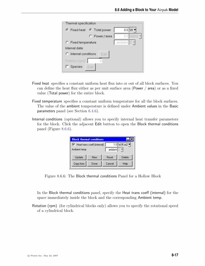
8.6 Adding a Block to Your Airpak Model
Fixed heat specifies a constant uniform heat flux into or out of all block surfaces. Youcan define the heat flux either as per unit surface area (Power / area) or as a fixedvalue (Total power) for the entire block.
Fixed temperature specifies a constant uniform temperature for all the block surfaces.The value of the ambient temperature is defined under Ambient values in the Basicparameters panel (see Section 6.4.6).
Internal conditions (optional) allows you to specify internal heat transfer parametersfor the block. Click the adjacent Edit button to open the Block thermal conditionspanel (Figure 8.6.6).
Figure 8.6.6: The Block thermal conditions Panel for a Hollow Block
In the Block thermal conditions panel, specify the Heat trans coeff (internal) for thespace immediately inside the block and the corresponding Ambient temp.
Rotation (rpm) (for cylindrical blocks only) allows you to specify the rotational speedof a cylindrical block.
c© Fluent Inc. May 22, 2007 8-17

Blocks
8-18 c© Fluent Inc. May 22, 2007

Chapter 9. Fans
Fans are two- or three-dimensional modeling objects. A fan is used to move fluid into,out of, or within the room. Fan geometries include circular, rectangular, inclined, and2D polygon. Fan types include fixed flow and characteristic curve. Fixed flow fans arealways located on a room wall and must be specified either as intake (drawing fluid intothe room) or exhaust (expelling fluid from the room). Characteristic curve fans can belocated anywhere within the room or on the room boundary.
Fans are always associated with a magnitude and direction of flow. Circular fans canpossess a central hub of non-zero radius and rectangular fans can have a rectangularhub. The hub is impervious to flow but can transfer heat to and from the fluid. Themagnitude of the flow can be specified either as a fixed value or as a function of pressuredrop across the fan.
In this chapter, information about the characteristics of a fan is presented in the followingsections:
• Section 9.1: Defining a Fan in Airpak
• Section 9.2: Geometry, Location, and Dimensions
• Section 9.3: Flow Direction
• Section 9.4: Fans in Series
• Section 9.5: Fans in Parallel
• Section 9.6: Fans on Blocks
• Section 9.7: Specifying Swirl
• Section 9.8: Fixed Flow
• Section 9.9: Fan Characteristic Curve
• Section 9.10: Adding a Fan to Your Airpak Model
c© Fluent Inc. May 22, 2007 9-1

Fans
9.1 Defining a Fan in Airpak
Figure 9.1.1 shows two fans on the room boundary; one defined as an intake fan and theother defined as an exhaust fan. The intake fan draws fluid into the room. By default,Airpak assumes that the intake fluid is at ambient temperature. The exhaust fan expelsfluid from the room in a direction determined by the local flow conditions. By default,the fluid exits the room at the temperature computed for the fluid within the room atthe intake side of the fan.
Figure 9.1.1: Intake and Exhaust Fans
Characteristic curve fans can be defined as exhaust, intake, or internal. Internal fans arelocated entirely within the room (see Figure 9.1.2) and are surrounded by fluid on allsides. The direction of flow through an internal 2D fan can be specified as positive ornegative, relative to the coordinate axis normal to the plane of the fan.
Figure 9.1.2: Internal Fan Placement
To configure a fan in the model, you must specify its geometry (including location anddimensions), its type, the flow rate associated with the fan, and the swirl. For a transientsimulation, you must also specify parameters related to the strength of the fan for acharacteristic curve fan. You can also specify the species concentrations and turbulenceparameters at the fan.
9-2 c© Fluent Inc. May 22, 2007

9.2 Geometry, Location, and Dimensions
9.2 Geometry, Location, and Dimensions
Fan location and dimension parameters vary according to fan geometry. Fan geometriesinclude circular, rectangular, inclined, cylindrical, and polygonal. These geometries aredescribed in Section 7.4.4.
9.2.1 Simple Fans
A simple fan is a two-dimensional fan that can have circular, rectangular, inclined, orpolygonal geometry.
A polygon fan is a two-dimensional fan. To create a 2D polygon fan, you should firstcreate a polygonal fan and then specify a height of zer.
Circular fans can include hubs. You must specify the size of the hub or inner radius (Intradius), and its overall size or outer radius (Radius), as shown in Figure 9.2.1.
Figure 9.2.1: Circular Fan Definition
Rectangular fans can also include a hub. To create a hub for a rectangular fan, you mustspecify the equivalent radius for the hub if it were to be created as a circular hub for acircular fan; i.e., you specify r in Figure 9.2.2.
Airpak will create a rectangular hub with the area πr2. Airpak uses the area of therectangular hub and the ratio of the lengths of the sides of the rectangular fan (d1 andl1 in Figure 9.2.2) to calculate the lengths of the sides of the rectangular hub (d2 and l2in Figure 9.2.2):
d2l2 = πr2 andd2
l2=d1
l1
If the fan is square, then d2 = l2 = x, and
c© Fluent Inc. May 22, 2007 9-3

Fans
Figure 9.2.2: Rectangular Fan Hub Definition
x2 = πr2 i.e., x =√πr
9.3 Flow Direction
Exhaust fans expel fluid from the room. The flow exits the room in a direction perpen-dicular to the fan.
By default, the direction of flow through an intake fan is normal to the plane of the fan.Airpak allows you to specify the flow direction for a fan and, thereby, model the effect ofof an inclided fan (see Figure 9.3.1).
Figure 9.3.1: Intake Fan Flow Direction
Internal fans can be located anywhere inside the room. Fluid flows through the fan in adirection perpendicular to it. You must specify the direction of flow (positive or negative)for an internal fan. For a rectangular, polygon, or circular fan, if flow is in the direction ofincreasing axis coordinates, the inward direction is positive. If flow is in the direction ofdecreasing coordinates, the inward direction is negative. For an inclined fan, the positive
9-4 c© Fluent Inc. May 22, 2007

9.3 Flow Direction
and negative directions are defined with respect to the axis of rotation for the inclinedfan:
• If the axis of rotation of the inclined fan is the x axis, the positive inward directionis the positive y direction, and the negative inward direction is the negative ydirection.
• If the axis of rotation of the inclined fan is the y axis, the positive inward directionis the positive z direction, and the negative inward direction is the negative zdirection.
• If the axis of rotation of the inclined fan is the z axis, the positive inward directionis the positive x direction, and the negative inward direction is the negative xdirection.
c© Fluent Inc. May 22, 2007 9-5

Fans
9.4 Fans in Series
Fans can be arranged in series (see Figure 9.4.1). There are two major advantages ofplacing several small fans in series rather than using a single large fan to achieve a givenflow rate:
• Fans placed in series can be made active and inactive individually, so you can createdifferent air flow patterns.
• Fans placed in series can direct air flows into localized streams.
Figure 9.4.1: Fans in Series
9.5 Fans in Parallel
Fans can also be positioned in parallel (see Figure 9.5.1). Two or more fans placed inparallel can increase flow with respect to a single fan of equivalent power.
Figure 9.5.1: Fans in Parallel
9-6 c© Fluent Inc. May 22, 2007

9.6 Fans on Blocks
9.6 Fans on Blocks
Fans can be combined with blocks to account for the dimensions of an actual fan. Thetreatment of fans used in conjunction with blocks varies according to the fan type. Whena hollow block is placed against a room wall to mask a region of the room, an ex-haust/intake fan can be positioned on any one of the exposed surfaces of the block (seeFigure 9.6.1). Fans used in this way must be exhaust/intake in type despite the fact thatthey are located within the room and not on a room wall, because, in effect, the interiorsurfaces of this block are room walls (i.e., they represent part of the room).
i Exhaust/intake fan and block combinations cannot involve a conducting solidblock.
Figure 9.6.1: Fan on a Block
Internal fans can be placed on any conducting solid block within the room to give thefan a thickness. Airpak will automatically “bore a hole” through the block on both sidesof the fan to allow fluid flow to and from the fan. Note that the face through which thefan bores a hole must not be located on the room boundary. Note that only conductingthick partitions and conducting solid blocks can be used for this purpose.
c© Fluent Inc. May 22, 2007 9-7

Fans
9.7 Specifying Swirl
To specify the swirl for a fan, you must specify the swirl magnitude or the rotationalspeed of the fan.
9.7.1 Swirl Magnitude
By default, Airpak assumes that fluid exits the fan in the direction normal to the plane ofthe fan. Alternatively, you can specify a swirl magnitude. This skews the flow directionin the θ direction (i.e., the direction of blade revolution). Swirl magnitude is defined by
uθ(r) = uz(r)(r
R
)S (9.7-1)
where uθ(r) is the velocity in the direction of revolution, uz(r) is the velocity in thedirection normal to the fan, r is the radial coordinate, R is the outer radius of the fan,and S is the swirl magnitude (S = 0 by default).
9.7.2 Fan RPM
Instead of using a specified swirl magnitude, Airpak can also allow the swirl factor tochange as a function of the operating point on the fan curve. This is achieved by specifyingthe RPM of the fan. The swirl magnitude (the ratio of the tangential velocity to theaxial velocity) can then change as the fan operating point changes on the fan curve. Forexample, if the flow rate through the fan decreases, the swirl magnitude will increase,and if the flow rate through the fan increases, the swirl magnitude will decrease. FanRPM is defined by
uθ(r) =[(RPM)× 2π
60× r
]1
20(9.7-2)
where r is the radial coordinate, and it is assumed that only 5% of the maximum tan-gential velocity of the fan is transferred to the fluid.
9.8 Fixed Flow
In real-world applications, the performance of a fan is described by its characteristiccurve, as described below. In Airpak, you can also specify a constant total mass flow orvolume flow rate.
9-8 c© Fluent Inc. May 22, 2007

9.9 Fan Characteristic Curve
9.9 Fan Characteristic Curve
The relationship between volumetric flow rate and the pressure drop across the fan (staticpressure) is described by the fan characteristic curve, which is usually supplied by thefan manufacturer. Figure 9.9.1 shows a characteristic curve for a common tube-axial fan.The total volumetric flow rate, Q, is plotted against fan static pressure, pfs.
Figure 9.9.1: Tube-axial Fan Curve
For a linear fan characteristic curve, only the volume flow rate at zero static pressure,Q0, and the fan static pressure at zero flow rate, p0, need to be specified. The equationfor a linear fan characteristic curve is
Q = Q0(p0 − pfs)/p0 (9.9-1)
In most cases, the linear characteristic curve does not adequately approximate the truefan characteristic curve over its entire operational range, so it is best to specify the actualfan curve, if possible.
Fan static pressure is computed by:
pfs = pdischarge − pintake (9.9-2)
where pintake is the pressure averaged over the face of the intake side of the fan, andpdischarge is the pressure averaged over the face of the discharge side of the fan.
For internal fans, both pintake and pdischarge are computed by Airpak. For an intake fan,pdischarge is computed by Airpak and pintake is the ambient pressure. The value of theambient pressure is specified under Ambient values in the Basic parameters panel (see Sec-tion 6.4.6). For an exhaust fan, pdischarge is the ambient pressure, and pintake is computedby Airpak. The default ambient pressure is zero (gauge pressure) and this should besatisfactory in almost all situations.
c© Fluent Inc. May 22, 2007 9-9

Fans
The accuracy of the fan flow rate used by Airpak is directly related to the accuracy withwhich the fan static pressure is computed. This, in turn, depends on how accuratelypressure losses in the entire system are modeled. Therefore, care should be taken tomodel all features of the system that contribute to the overall nature of the pressuredistribution in the system.
You can create a report of the fan operating point (pressure rise and volume flow rate)for a characteristic curve fan, as described in Section 29.8.
9-10 c© Fluent Inc. May 22, 2007

9.10 Adding a Fan to Your Airpak Model
9.10 Adding a Fan to Your Airpak Model
To include a fan in your Airpak model, click on the button in the Object creation
toolbar and then click on the button to open the Fans panel, shown in Figures 9.10.1and 9.10.2.
Figure 9.10.1: The Fans Panel (Geometry Tab)
The procedure for adding a fan to your Airpak model is as follows:
1. Create a fan. See Section 7.3.2 for details on creating a new object and Section 7.3.9
c© Fluent Inc. May 22, 2007 9-11

Fans
for details on copying an existing object.
2. Change the description of the fan, if required. See Section 7.4.1 for details.
3. Change the graphical style of the fan, if required. See Section 7.4.2 for details.
4. In the Info tab, enter the Manufacturer and Model number, if known.
5. Specify the geometry, position, and size of the fan in the Geometry tab. Thereare five different kinds of geometry available for fans in the Shape drop-down listfor fans. The inputs for these geometries are described in Section 7.4.4. See Sec-tion 7.3.6 for details on resizing an object and Section 7.3.7 for details on reposi-tioning an object.
A polygon fan can be two-dimensional or three-dimensional. To create a 3D polygonfan, select Polygon in the Fans panel and specify a non-zero Height. To create a 2Dpolygon fan, select Polygon and specify a Height of zero.
i Note that if you specify a circular fan, you can specify the size of the hubor inner radius (IRadius). If you specify a rectangular fan, you can specify theequivalent radius for the rectangular hub (Internal hub equiv. radius).
6. In the Properties tab, select the Fan type.. This will specify whether the fan is onthe room boundary or inside the room. There are different options for Fixed flowand Characteristic curve fans.
Exhaust specifies that the fan is an exhaust fan. For 2D and 3D fans, the fluid isdefined to exit the room through the fan in a direction determined by the localflow conditions. You do not need to specify a flow direction for an exhaustfan.
Intake specifies that the fan is an intake fan. The following inputs are requiredfor an intake fan.
(a) Specify the Fluid temp. This is the temperature of the fluid being drawninto the model, and is specified as ambient by default. The value of theambient temperature is defined under Ambient values in the Basic param-eters panel (see Section 6.4.6).
(b) (2D fans only) Specify the flow direction. . There are two options:
• If the fluid flows into the room normal to the fan, select Normal.
• To specify the flow angle of the fluid entering the room through thefan, select Given. There are two options:
Vector allows you to specify the direction vector (X, Y, Z) for theflow. Only the direction of the vector is used by Airpak; the magni-tude is ignored.
9-12 c© Fluent Inc. May 22, 2007

9.10 Adding a Fan to Your Airpak Model
Angles allows you to specify the direction of the flow entering theroom in terms of angles relative to the inward-pointing normal di-rection. You can specify two angles, A (α) and T (θ), to account forincoming flow not aligned with the normal direction. If the normalinward vector points in the positive direction, then α and θ musthave values in the range −90 < angle < 90, with α=θ=0 repre-senting flow in the positive normal direction. If the normal inwardvector points in the negative direction, then α and θ must have val-ues in the range 90 < angle < 270, with α=θ=180 representingflow in the negative normal direction. Since the fan may be orientedin any one of three planes (x-y, y-z, or x-z), the roles of α and θwill vary depending on the orientation of the plane of the fan. Anexample is shown in Figure 9.10.3, where the fan is in the x-y planeand the normal inward vector is pointing in the positive direction.
Internal (2D characteristic curve fans only) specifies that the fan is an internalfan. Specify the Facing direction of the intake relative to the normal direction.The Positive and Negative options specify the inward direction normal to thefan as pointing toward high or low coordinates, respectively.
7. Specify the Flow rate for the fan. There are different options for the fixed flow andcharacteristic curve fans.
• For a fixed flow fan, you can specify a Volume flow rate or a Mass flow rate.
• for a characteristic curve fan, the following options are available:
Linear allows you to specify values defining a linear fan curve. Specify theVolume flow rate at zero fan static pressure, and a static pressure at zeroflow (Static pressure (head)). The value of the ambient pressure is definedunder Ambient values in the Problem setup panel (see Section 6.4.6).
Curve allows you to define the characteristic curve as a curve consistingof piecewise-continuous line segments. Airpak allows you to describe thecurve either by positioning a series of points on a graph using the Fan curvegraphics display and control window (described below), or by specifyinga list of fan static pressure/volume flow rate coordinate pairs using theCurve specification panel (described below). These options are availableunder Edit.
To load a previously defined curve, click Load. This will open the Loadcurve file selection dialog box. Select the file containing the curve dataand click Accept. See Section 2.1.8 for details on selecting a file.
To save a curve, click Save. This will open the Save curve dialog box, andyou can specify the filename and directory where the curve data is to besaved.
c© Fluent Inc. May 22, 2007 9-13

Fans
i Note that the box to the right of Edit will be empty if you have notdefined a curve for the fan. This box will contain the first volume flowvalue if you have defined a curve.
8. (characteristic curve fans only) Specify the Transient strength. This option is avail-able only if you have selected Transient under Time variation in the Basic parameterspanel. To edit the transient parameters for the fan, click Edit next to Transientstrength. See Chapter 20 for details on transient simulations.
9. Specify the Swirl for the fan. You can specify a Magnitude or RPM for the fan.
10. Specify the inlet or outlet species concentrations for the fan, if required. SelectSpecies and click the Edit button to open the Species concentrations panel (Fig-ure 21.2.4). For details on setting species parameters, see Chapter 21.
11. Specify the turbulence parameters for the fan, if required. This option is availableonly if you selected the Two equation or RNG k-ε model in the Basic parameters panel(Figure 6.4.1). See Section 6.4.3 for details on determining turbulence parametersfor objects in your Airpak model.
Select Turbulence in the Fans panel and click Edit to open the Turbulence equationparameters panel (Figure 9.10.4).
There are two options for specifying turbulence parameters:
Turbulent intensity/turbulent length scale allows you to specify the turbulence in-tensity and length scale for the fan.
Specify values for the Turbulent intensity and the Turbulent length scale. Thedefault value of the turbulence intensity is 10%. By default, Airpak will usea default value for the length scale. The default value calculated by Airpak is10% of the length of the shortest side of the fan.
Turbulent energy/turbulent dissipation allows you to specify the Turbulent energyand Turbulent dissipation rate for the fan.
12. Specify the Solar behavior for the fan. This option is available if you have enabledsolar loading in the Basic parameters panel. See Section 22.5 for details.
9.10.1 Using the Fan curve Window to Specify the Curve for a CharacteristicCurve Fan Type
You can specify a curve for a Characteristic curve fan type using the Fan curve graphicsdisplay and control window (Figure 9.10.5). To open the Fan curve window, select Curveunder Characteristic curve in the Fans panel and click on Edit. Select Graph editor fromthe resulting list.
The following functions are available for creating, editing, and viewing a curve:
9-14 c© Fluent Inc. May 22, 2007

9.10 Adding a Fan to Your Airpak Model
• To create a new point on the curve, click on the curve with the middle mousebutton.
• To move a point on the curve, hold down the middle mouse button while positionedover the point, and move the mouse to the new location of the point.
• To delete a point on the curve, click the right mouse button on the point.
• To zoom into an area of the curve, position the mouse pointer at a corner of thearea to be zoomed, hold down the left mouse button and drag open a selection boxto the desired size, and then release the mouse button. The selected area will thenfill the Fan curve window, with appropriate changes to the axes. After you havezoomed into an area of the model, click on Full range to restore the graph to itsoriginal axes and scale.
• To set the minimum and maximum values for the scales on the axes, click on Setrange. This will open the Set range panel (Figure 9.10.6).
Enter values for Min X, Min Y, Max X, and Max Y and click Accept.
• To load a previously defined curve, click on Load. This will open the Load curvefile selection dialog box. Select the file containing the curve data and click Accept.See Section 9.10.2 for details about creating a curve file outside of Airpak. SeeSection 2.1.8 for details on selecting a file.
• To save a curve, click on Save. This will open the Save curve dialog box, in whichyou can specify the filename and directory to which the curve data is to be saved.
You can use the Print button to print the curve. See Section 3.5 for details on savinghardcopy files.
Click Done when you have finished creating the curve; this will store the curve and closethe Fan curve window. Once the curve is defined, you can view the pairs of coordinatesdefining the curve in the Curve specification panel. See Figure 9.10.7 for the pairs ofcoordinates for the curve shown in Figure 9.10.5.
i Note that the curve you specify must intersect both the x and y axes.
9.10.2 Using the Curve specification Panel to Specify the Curve for aCharacteristic Curve Fan Type
You can define a curve for a Characteristic curve fan type using the Curve specification panel(Figure 9.10.7). To open the Curve specification panel, select Curve under Characteristiccurve in the Fans panel and click on Edit. Select Text editor from the resulting list.
c© Fluent Inc. May 22, 2007 9-15

Fans
To define a curve, specify a list of coordinate pairs in the Curve specification panel.It is important to give the numbers in pairs, but the spacing between numbers is notimportant. Click Accept when you have finished entering the pairs of coordinates; thiswill store the values and close the Curve specification panel.
To load a previously defined curve, click on Load. This will open the Load curve fileselection dialog box. Select the file containing the curve data and click Accept. SeeSection 2.1.8 for details on selecting a file. If you know the units used in the curve datayou are loading, you should select the appropriate units in the Curve specification panelbefore you load the curve. If you want to view the imported data after you have loadedthem, using different units than the default units in the Curve specification panel, selectFix values for Volume flow units and/or Pressure units and select the appropriate unitsfrom the unit definition list.
If you want to load a curve file that you have created outside of Airpak, you will needto make sure that the first three lines of the file before the data contain the followinginformation:
1. the number of data sets in the file (usually 1)
2. the unit specifications for the file, which can be obtained from the Curve specificationpanel (e.g., units m3/s N/m2)
3. the number of data points in the file (e.g., 10)
Using the above example, the first three lines of the curve file would be
1
units m3/s N/m2
10
The actual data points should be entered in the same was as you would enter them inthe Curve specification panel.
i If you want to load a curve from an Excel file, make sure that you also save thefile as formatted text (space delimited) before reading it into Airpak.
To save a curve, click on Save. This will open the Save curve dialog box, in which youcan specify the filename and directory to which the curve data is to be saved.
Once the pairs of coordinates have been entered, you can view the curve in the Fan curvegraphics display and control window. See Figure 9.10.5 for the curve for the values shownin Figure 9.10.7.
9-16 c© Fluent Inc. May 22, 2007

9.10 Adding a Fan to Your Airpak Model
Figure 9.10.2: The Fans Panel (Properties Tab)
c© Fluent Inc. May 22, 2007 9-17

Fans
X
Y
Z
FanFlow direction
XY
Z
Fan
Flowdirection
Normaldirection
Normaldirectionα
θ
Figure 9.10.3: Definition of Angles for a Fan
Figure 9.10.4: The Turbulence equation parameters Panel
9-18 c© Fluent Inc. May 22, 2007

9.10 Adding a Fan to Your Airpak Model
Figure 9.10.5: The Fan curve Graphics Display and Control Window
Figure 9.10.6: The Set range Panel
c© Fluent Inc. May 22, 2007 9-19

Fans
Figure 9.10.7: The Curve specification Panel
9-20 c© Fluent Inc. May 22, 2007

Chapter 10. Vents
10.1 Overview
Vents represent holes through which fluid can enter or leave the room. They are alwayslocated on enclosure boundaries (i.e., either room walls or the surfaces of blocks used tomodify the shape of the room) See Figure 10.1.1. Vent geometries include rectangular,circular, 2D polygon, and inclined.
Rectangular inletvent on a block
Circular inletvent on a block
Circularinlet vent
Rectangularoutlet vent
Figure 10.1.1: Vent Examples
In most real-world cases, vents have coverings (e.g., screen meshes, angled slats, wirevents). These coverings result in a pressure drop across the plane of the vent. Airpaktreats the pressure drop in the same way that it treats a pressure drop through a resistancemodeling object.
Fluid can enter or exit the room through a vent. The actual flow direction through thevent is computed by Airpak. In some cases, fluid can enter and exit through differentareas of a single vent. In cases where the amount of flow in both directions is nearlyequal, the vent may be modeled as two separate but adjoining vents.
Airpak computes both the temperature and the direction of the fluid exiting the roomthrough a vent. By default, the temperature of the fluid entering the room through avent is assumed to be the ambient temperature specified under Ambient values in theBasic parameters panel (see Section 6.4.6). If flow is leaving the domain through the vent,the temperature is ignored. By default, the direction of flow of the fluid through a ventis computed by Airpak. If you know the direction of flow at the vent, you can specify itin the Vents panel.
c© Fluent Inc. May 22, 2007 10-1

Vents
To configure a vent in the model, you must specify its geometry (including location anddimensions). For best results, the vent size and geometry should closely match the sizeand geometry of the actual vent. In some cases, you must also specify the temperature,pressure, species concentration, turbulence parameters, and/or method used to calculatethe pressure drop through the vent covering.
10.2 Planar Resistances
Planar resistances represent partial obstructions to flow within the room. Planar resis-tance geometries include rectangular, circular, inclined, and 2D polygon and are designedto model planar flow obstructions such as screens and permeable baffles.
For a planar resistance in Airpak, the effect of any resistance is modeled as a pressuredrop through its area or volume. Airpak provides a list of resistance types that youcan select to model the pressure drop through a planar resistance. Alternatively, thepressure drop across the resistance can be calculated using either the approach-velocitymethod or the device-velocity method, both of which require a user-specified velocity losscoefficient. The approach-velocity and device-velocity methods differ from each otheronly by virtue of a factor called the free area ratio. The calculated pressure drop canbe proportional either to the fluid velocity itself, or to the square of the velocity. It iscommon practice to employ the linear relationship for laminar flow and the quadraticrelationship for turbulent flow. In the general case, a combination of the linear andquadratic relationships may more accurately model the pressure drop/speed curve.
10-2 c© Fluent Inc. May 22, 2007

10.3 Geometry, Location, and Dimensions
i Note that you cannot use the hexahedral mesher if a planar resistance is placed onan inclined conducting thick partition. The tetrahedral mesher, on the other hand,can be used with all types of resistances.
To configure a flow resistance in the model, you must specify its geometry (including lo-cation and dimensions), the pressure drop model, and the relationship between resistanceand velocity.
10.3 Geometry, Location, and Dimensions
Vent location and dimension parameters vary according to the vent geometry. Ventgeometries include rectangular, circular, inclined, and 2D polygon. These geometries aredescribed in Section 7.4.4.
10.4 Pressure Drop Calculations for Vents
Airpak computes the speed, direction, and temperature of the fluid exiting the roomthrough a vent (see Figure 10.4.1). The calculations are based on the assumption thatthe external pressure is static. If you do not specify a value for the external pressure,Airpak uses the ambient pressure specified under Ambient values in the Basic parameterspanel (see Section 6.4.6).
X
Y
Z
Ambientpressure Vent
Temperature of fluid leavingis the same as the temperatureof the fluid inside adjacent to the exit.
Figure 10.4.1: Outlet Vent Conditions
Fluid entering the room through a vent is drawn in from the external environment. Bydefault, the external fluid is at the ambient temperature specified under Ambient values inthe Basic parameters panel (see Section 6.4.6), and the flow enters the room in a directioncomputed by Airpak. However, you can impose a flow direction, as shown in Figure 10.4.2.You can also specify a temperature for the fluid entering the vent.
c© Fluent Inc. May 22, 2007 10-3

Vents
Defaultdirectionnormalto vent
Inlet flownormal tovent
Enclosureside
Externalenvironmentside
Flow directionspecifiedby user
Enclosureside
Externalenvironmentside
Inlet flownot normalto vent
Figure 10.4.2: Vent Flow Direction
To account for pressure losses due to the presence of mesh screens or angled slats on thevent, you must specify a loss coefficient or select a vent type. See [14] for a compilationof loss coefficients applicable to most situations encountered in electronic enclosures.
Airpak can calculate loss coefficients for different types of vents based on the free arearatio of the vent. The following vent types are available in Airpak:
• a perforated thin vent, with a loss coefficient of
lc =1
A2
[0.707(1− A)0.375 + 1− A
]2(10.4-1)
where A is the free area ratio.
• a circular metal wire screen, with a loss coefficient of
lc = 1.3(1− A) +(
1
A− 1
)2
(10.4-2)
where A is the free area ratio.
• a two-plane screen with cylindrical bars, with a loss coefficient of
lc =1.28(1− A)
A2(10.4-3)
where A is the free area ratio.
10-4 c© Fluent Inc. May 22, 2007

10.4 Pressure Drop Calculations for Vents
i Note that setting the ambient temperature and flow direction has no effect on thecalculations if fluid flows out of the room through the vent.
Alternatively, Airpak can calculate the pressure drop resulting from a resistance either bythe approach-velocity method or by the device-velocity method.
The approach-velocity method relates the pressure drop to the fluid velocity:
∆p = ρlc12vnapp (10.4-4)
where lc is the user-specified loss coefficient, ρ is the fluid density, and vapp is the approachvelocity. The approach velocity is the calculated velocity at the plane of the vent. Thevelocity dependence can be linear (n = 1), quadratic (n = 2), or a combination of linearand quadratic.
The device-velocity method relates the pressure drop induced by the vent to the fluidvelocity:
∆p = ρlc22vndev (10.4-5)
where vdev is the device velocity. The velocity dependence can be linear (n = 1), quadratic(n = 2), or a combination of linear and quadratic.
The difference between the approach-velocity and device-velocity methods is in the ve-locity used to compute the pressure drop. The device velocity is related to the approachvelocity by
vdev =vapp
A(10.4-6)
where A is the free area ratio. The free area ratio is the ratio of the area through whichthe fluid can flow unobstructed to the total planar area of the obstruction.
i Note that the loss coefficient used in the equation for the device velocity is not thesame as the loss coefficient used in the equation for the approach velocity.
c© Fluent Inc. May 22, 2007 10-5

Vents
The loss coefficients in Equations 10.4-4 and 10.4-5 are related to the flow regime of theproblem:
• For a viscous flow regime (e.g., laminar flow, slow flow, very dense packing), youshould select a linear velocity relationship:
∆p =ρ
2lc1v (10.4-7)
• For an inertial flow regime (e.g., turbulent flow), you should select a quadraticvelocity relationship:
∆p =ρ
2lc2v
2 (10.4-8)
• For a combination of these two types of flow, you should select a linear+quadraticvelocity relationship:
∆p = ∆plinear + ∆pquadratic (10.4-9)
You can obtain the loss coefficients in several ways:
• experimental measurements
• computational measurements
• from a reference (The loss coefficients for many vent configurations are available in[14].)
10.5 Adding a Vent to Your Airpak Model
To include a vent in your Airpak model, click on the button in the Object creation
toolbar and then click on the button to open the Vents panel, shown in Figures 10.5.1– 10.5.3.
The procedure for adding a vent to your Airpak model is as follows:
1. Create a vent. See Section 7.3.2 for details on creating a new object and Sec-tion 7.3.9 for details on copying an existing object.
2. Change the description of the vent, if required. See Section 7.4.1 for details.
3. Change the graphical style of the vent, if required. See Section 7.4.2 for details.
10-6 c© Fluent Inc. May 22, 2007

10.5 Adding a Vent to Your Airpak Model
Figure 10.5.1: The Vents Panel (Geometry Tab)
c© Fluent Inc. May 22, 2007 10-7

Vents
Figure 10.5.2: The Vents Panel (Properties Tab) for an External Vent
10-8 c© Fluent Inc. May 22, 2007

10.5 Adding a Vent to Your Airpak Model
Figure 10.5.3: The Vents Panel (Properties Tab) for an Internal 2D ResistanceVent
c© Fluent Inc. May 22, 2007 10-9

Vents
4. In the Geometry tab, specify the geometry, position, and size of the vent (Fig-ure 10.5.1). There are four different kinds of geometry available for vents in theShape drop-down list. The inputs for these geometries are described in Section 7.4.4.See Section 7.3.6 for details on resizing an object and Section 7.3.7 for details onrepositioning an object.
5. In the Properties tab, specify the characteristics for the vent.
(a) Specify the Vent type as Internal (Figure 10.5.3) or External (Figure 10.5.2).Choose Internal for a 2D resistance vent.
(b) (Internal and External Vents) Select the Loss specification in the drop-down list.The following options are available:
• To specify the loss coefficient, select Loss coefficient and then select themethod to be used to calculate the velocity loss coefficient. The followingoptions are available in the Velocity loss coefficient drop-down list.
– To have Airpak calculate the loss coefficient for a particular vent typebased on the free area ratio of the vent, select Automatic. Then selectthe type of vent (Perforated thin vent, Circular metal wire screen, orTwo-plane screen, cyl. bars) in the Resistance type drop-down list andspecify the Free area ratio.
– To use the device-velocity method, select Device and select the methodto be used to calculate the Resistance velocity dependence. Thereare three options in the drop-down list: Linear, Quadratic, and Lin-ear+quadratic. Finally, specify the appropriate Loss coefficient andFree area ratio for the Linear coeff. and/or Quadratic coeff..
– To use the approach-velocity method, select Approach and select themethod to be used to calculate the Resistance velocity dependence.Finally, specify the appropriate Loss coefficient for the Linear coeff.and/or Quadratic coeff.
• To define a piecewise-linear profile for the pressure drop as a function ofthe speed of the fluid through the vent, select Loss curve. Airpak allowsyou to describe the curve either by positioning a series of points on a graphusing the Resistance curve graphics display and control window (describedbelow), or by specifying a list of vent speed/pressure coordinate pairsusing the Curve specification panel (described below). These options areavailable under Edit.
To load a previously defined curve, click on Load. This will open the Loadcurve file selection dialog box. Select the file containing the curve dataand click Accept. See Section 2.1.8 for details on selecting a file.
To save a curve, click on Save. This will open the Save curve dialog box,in which you can specify the filename and directory to which the curvedata is to be saved.
10-10 c© Fluent Inc. May 22, 2007

10.5 Adding a Vent to Your Airpak Model
i Note that the box to the right of Edit will be empty if you havenot defined a curve for the vent. This box will contain the first speedvalue if you have defined a curve.
The following parameters can be set for External vents, only.
(c) Enter a value for the Ambient temperature of the external fluid. The defaultvalue of Ambient temperature is the ambient temperature specified under Am-bient values in the Basic parameters panel (see Section 6.4.6). This temperatureis used if fluid flows into the room through the vent, and is ignored if fluidflows out of the room through the vent.
(d) To specify the external pressure, enter a value for the Pressure (stagnation/static).For flow into a vent, the external pressure is the stagnation pressure. For flowout of a vent, the external pressure is the static pressure. By default, theexternal pressure is the ambient pressure specified under Ambient values in theBasic parameters panel (see Section 6.4.6).
(e) Specify the Flow direction. There are three options:
• If the fluid flows into the room normal to the vent, select Normal in.
• If the fluid flows out of the room normal to the vent, select Normal out.
• To specify the flow angle of the fluid entering the room through the vent,select Given. There are two options:
Vector allows you to specify the direction vector (X, Y, Z) for the flow.Only the direction of the vector is used by Airpak; the magnitude isignored.
Angles allows you to specify the direction of the flow entering the roomin terms of angles relative to the inward-pointing normal direction.You can specify two angles, A (α) and T (θ), to account for incomingflow not aligned with the normal direction. If the normal inwardvector points in the positive direction, then α and θ must have valuesin the range −90 < angle < 90, with α=θ=0 representing flow inthe positive normal direction. If the normal inward vector points inthe negative direction, then α and θ must have values in the range90 < angle < 270, with α=θ=180 representing flow in the negativenormal direction. Since the vent may be oriented in any one of threeplanes (x-y, y-z, or x-z), the roles of α and θ will vary dependingon the orientation of the plane of the vent. An example is shownin Figure 10.5.4, where the vent is in the x-y plane and the normalinward vector is pointing in the positive direction.
(f) Specify the inlet or outlet species concentrations for the vent, if required. Youcan input the species concentrations for the vent using the Species concentra-tions panel. To open this panel, select Species in the Vents panel and thenclick Edit. See Chapter 21 for details on modeling species transport.
c© Fluent Inc. May 22, 2007 10-11

Vents
X
Y
Z
VentFlow direction
XY
Z
Vent
Flowdirection
Normaldirection
Normaldirectionα
θ
Figure 10.5.4: Definition of Angles for a Vent
(g) Specify the turbulence parameters for the vent, if required. This option isavailable only if you selected the Two equation or RNG k-ε model in the Basicparameters panel (Figure 6.4.1). See Section 6.4.3 for details on determiningturbulence parameters for objects in your Airpak model.
Select Turbulence in the Vents panel and click Edit to open the Turbulenceequation parameters panel (Figure 10.5.5).
Figure 10.5.5: The Turbulence equation parameters Panel
There are two options for specifying turbulence parameters:
Turbulent intensity/turbulent length scale allows you to specify the turbu-lence intensity and length scale for the vent.
Specify values for the Turbulent intensity and the Turbulent length scale.The default value of the turbulence intensity is 10%. By default, Airpakwill use a default value for the length scale. The default value calculatedby Airpak is 10% of the length of the shortest side of the vent.
10-12 c© Fluent Inc. May 22, 2007

10.5 Adding a Vent to Your Airpak Model
Turbulent energy/turbulent dissipation allows you to specify the Turbulentenergy and Turbulent dissipation rate for the vent.
(h) If you have enabled solar loading in the Basic parameters panel, specify theSolar behavior for the vent. See Section 22.5 for details.
10.5.1 Using the Resistance curve Window to Specify the Curve for a Vent
You can specify a resistance curve for a vent using the Resistance curve graphics displayand control window (Figure 10.5.6). To open the Resistance curve window, select Losscurve from the Loss specification drop-down list in the Vents panel and click on Edit.Select Graph editor from the resulting list.
The following functions are available for creating, editing, and viewing a curve:
• To create a new point on the curve, click on the curve with the middle mousebutton.
• To move a point on the curve, hold down the middle mouse button while positionedover the point, and move the mouse to the new location of the point.
• To delete a point on the curve, click the right mouse button on the point.
• To zoom into an area of the curve, position the mouse pointer at a corner of thearea to be zoomed, hold down the left mouse button and drag open a selection boxto the desired size, and then release the mouse button. The selected area will thenfill the Resistance curve window, with appropriate changes to the axes. After youhave zoomed into an area of the model, click on Full range to restore the graph toits original axes and scale.
• To set the minimum and maximum values for the scales on the axes, click on Setrange. This will open the Set range panel (Figure 10.5.7).
Enter values for Min X, Min Y, Max X, and Max Y and click Accept.
• To load a previously defined curve, click on Load. This will open the Load curvefile selection dialog box. Select the file containing the curve data and click Accept.See Section 2.1.8 for details on selecting a file.
• To save a curve, click on Save. This will open the Save curve dialog box, in whichyou can specify the filename and directory to which the curve data is to be saved.
You can use the Print button to print the curve. See Section 3.5 for details on savinghardcopy files. Click Done when you have finished creating the curve; this will store thecurve and close the Resistance curve window. Once the curve is defined, you can view thepairs of coordinates defining the curve in the Curve specification panel. See Figure 10.5.8for the pairs of coordinates for the curve shown in Figure 10.5.6.
c© Fluent Inc. May 22, 2007 10-13

Vents
Figure 10.5.6: The Resistance curve Graphics Display and Control Window
Figure 10.5.7: The Set range Panel
10-14 c© Fluent Inc. May 22, 2007

10.5 Adding a Vent to Your Airpak Model
i Note that the curve you specify must intersect both the x and y axes.
10.5.2 Using the Curve specification Panel to Specify the Curve for a Vent
You can define a resistance curve for a vent using the Curve specification panel (Fig-ure 10.5.8). To open the Curve specification panel, select Loss curve from the Loss speci-fication drop-down list in the Vents panel and click on Edit. Select Text editor from theresulting list.
Figure 10.5.8: The Curve specification Panel
To define a curve, specify a list of coordinate pairs in the Curve specification panel.It is important to give the numbers in pairs, but the spacing between numbers is notimportant. Click Accept when you have finished entering the pairs of coordinates; thiswill store the values and close the Curve specification panel.
To load a previously defined curve, click on Load. This will open the Load curve fileselection dialog box. Select the file containing the curve data and click Accept. SeeSection 2.1.8 for details on selecting a file. If you know the units used in the curve datayou are loading, you should select the appropriate units in the Curve specification panelbefore you load the curve. If you want to view the imported data after you have loadedthem, using different units than the default units in the Curve specification panel, selectFix values for Speed units and/or Pressure units and select the appropriate units from theunit definition list.
If you want to load a curve file that you have created outside of Airpak, you will needto make sure that the first three lines of the file before the data contain the followinginformation:
c© Fluent Inc. May 22, 2007 10-15

Vents
1. the number of data sets in the file (usually 1)
2. the unit specifications for the file, which can be obtained from the Curve specificationpanel (e.g., units m/s N/m2)
3. the number of data points in the file (e.g., 10)
Using the above example, the first three lines of the curve file would be
1
units m/s N/m2
10
The actual data points should be entered in the same was as you would enter them inthe Curve specification panel.
i If you want to load a curve from an Excel file, make sure that you also save thefile as formatted text (space delimited) before reading it into Airpak.
To save a curve, click on Save. This will open the Save curve dialog box, in which youcan specify the filename and directory to which the curve data is to be saved.
Once the pairs of coordinates have been entered, you can view the curve in the Resistancecurve graphics display and control window. See Figure 10.5.6 for the curve for the valuesshown in Figure 10.5.8.
10-16 c© Fluent Inc. May 22, 2007

Chapter 11. Openings
Openings are two-dimensional modeling objects representing areas of the model throughwhich fluid can flow. Opening geometries include rectangular, circular, 2D polygon,and inclined. Opening types include free and recirculation. Free openings are specifiedindividually, but recirculation openings must be specified in pairs. Recirculation openingpairs consist of two sections:
• an extract section, representing the location at which fluid is removed from theenclosure
• a supply section, representing the location at which fluid is returned to the enclosure
Openings should be located on an enclosure boundary (i.e., either a room wall or thesurface of a hollow block that has been used to mask a portion of the enclosure). Freeopenings can also be located on the surfaces of blocks or partitions within the room.
Free openings represent holes either on the boundary of the room or on blocks or parti-tions. Recirculation openings model devices (e.g., heaters, refrigeration circuits, or filters)that extract fluid from the room at one location, and supply it to a different location inthe model with altered thermal or species properties.
Note that the mass flow rates for the extract and supply sections of a recirculationopening must be the same. You can specify different mass fluxes for the two sections ifthey differ in size, but the mass flow rates (mass flux × area) for the sections must bethe same.
To configure an opening in the model, you must specify its geometry (including locationand dimensions) and type. For free openings, you can also specify temperature, staticpressure, species concentrations, velocity, and turbulence parameters at the opening.For transient problems, you can specify the variation of temperature, pressure, speciesconcentration, velocity, and turbulence parameters with time. For recirculation openings,you must specify the mass flow rate and thermal treatment of the fluid in the recirculationloop. The thermal treatment can be specified as a constant temperature increase (ordecrease), a fixed heat input (or extraction), or using a conductance and the externaltemperature. You can also specify the direction of flow out of the supply section as wellas an increase or decrease in species in the recirculation loop.
c© Fluent Inc. May 22, 2007 11-1

Openings
In this chapter, information about the characteristics of an opening is presented in thefollowing sections:
• Section 11.1: Geometry, Location, and Dimensions
• Section 11.2: Free Openings
• Section 11.3: Recirculation Openings
• Section 11.4: Adding an Opening to Your Airpak Model
11.1 Geometry, Location, and Dimensions
The location and dimension parameters for an opening vary according to the geometry ofthe opening. Opening geometries include rectangular, circular, 2D polygon, and inclined.These geometries are described in Section 7.4.4.
i The geometries of the extract and supply sections for a recirculation opening candiffer from one another.
11.2 Free Openings
A free opening represents an area on the surface of a solid object (e.g., block, partition),or an area on a planar object such as a wall, through which a fluid is free to flow inany direction. In most cases, an opening represents a hole on the boundary of the roomwhere the model fluid is exposed to the external environment.
By default, Airpak calculates the rate of flow through a free opening as part of the solution.
For free openings located on room walls, Airpak computes the rate of flow through theopening based on an external static pressure. The default external pressure and temper-ature are the ambient temperature specified under Ambient values in the Basic parameterspanel (see Section 6.4.6). For cases where the external fluid velocity is not perpendicularto the plane of the opening, Airpak also allows you to specify the velocity directionalcomponents as well as specify species concentrations and turbulence parameters at theopening. In addition, you can specify boundary profiles for pressure, temperature, veloc-ity, species concentrations, and turbulence parameters at a free opening.
11-2 c© Fluent Inc. May 22, 2007

11.3 Recirculation Openings
11.3 Recirculation Openings
Recirculation openings model recirculation devices such as heating or cooling units. Insuch a device, the fluid is withdrawn from the room through the extract section of theopening and returned to the room through the supply section, as shown in Figure 11.3.1.The extract and supply sections of the recirculation opening can differ from one anotherin both size and geometry.
Room
Recirculation device
ExtractSupply
Heat extracted/supplied or species filtered
Figure 11.3.1: External Recirculation Cooling Device
You can model an internal recirculation device by placing the extract and supply sec-tions of a recirculation opening on two different sides of an adiabatic block, as shown inFigure 11.3.2.
i A conducting solid block cannot be used to represent an internal recirculationdevice.
Figure 11.3.2: Internal Recirculation Device
c© Fluent Inc. May 22, 2007 11-3

Openings
11.3.1 Recirculation Mass Flow Rate
Airpak provides three methods of specifying the flow rate through a recirculation device:
• total mass flow through the opening
• mass flow rate per unit area of the opening
• total volumetric flow throught the opening
Because the extract and supply sections can differ in size, the per-unit-area specificationcan result in different mass fluxes but the same mass flow rate for each section of theopening. Such specifications can be used to model devices that extract or supply a fluidanywhere in the recirculation loop.
11.3.2 Flow Direction for Recirculation Openings
By default, the flow direction of the fluid passing through the extract or supply sectionof a recirculation opening is normal to the plane of the section. However, you can specifythat the flow leaves the supply section at an angle, as shown in Figure 11.3.3. Note thatAirpak uses the direction parameters only to determine the direction of fluid flow; theydo not affect the magnitude of the velocity.
Defaultdirectionnormalto opening
Inlet flownormal toopening
Enclosureside
Externalenvironmentside
Flow directionspecifiedby user
Enclosureside
Flow not normalto opening
Externalenvironmentside
Figure 11.3.3: Flow Direction Through Opening Section
11.3.3 Recirculation Opening Thermal Specifications
When fluid exits and re-enters the enclosure through a recirculation device, its temper-ature can increase or decrease. Airpak computes the temperature of the re-entering fluid
11-4 c© Fluent Inc. May 22, 2007

11.3 Recirculation Openings
(Tsupply) based on the temperature of the exiting fluid (Textract) and the thermal changeapplied to the fluid as it passes through the device.
Airpak provides three methods for computing Tsupply. The first method requires thespecification of a constant temperature change (∆T ) applied to the fluid within thedevice. In this case, Tsupply is computed by
Tsupply = Textract + ∆T (11.3-1)
where Textract is the temperature of the enclosure fluid averaged over the face of theextract section.
The second method requires the specification of the amount of heat (∆H) input to orextracted from the fluid by the recirculation device. In this case, Tsupply is computed by
Tsupply = Textract +∆H
cpm(11.3-2)
where cp is the fluid specific heat of the default fluid material selected in the Basicparameters panel (see Section 6.4.7) and m is the mass flow rate through the device.
The third method requires the specification of the conductance (h1A) and the externaltemperature (Texternal). In this case, Tsupply is computed by
Tsupply = Textract −h1A(Textract − Texternal)
cpm(11.3-3)
where cp is the specific heat of the default fluid material selected in the Basic parameterspanel (see Section 6.4.7), and m is the mass flow rate through the device.
11.3.4 Recirculation Opening Species Filters
When fluid exits and re-enters the room through a recirculation device, you can specifyan increase or decrease of species in the recirculation loop. See Chapter 21 for details onmodeling species transport.
c© Fluent Inc. May 22, 2007 11-5

Openings
11.4 Adding an Opening to Your Airpak Model
To include an opening in your Airpak model, click on the button in the Object
creation toolbar and then click on the button to open the Openings panel, shown inFigures 11.4.1 and 11.4.2.
Figure 11.4.1: The Openings Panel for a Free Opening (Geometry Tab)
The procedure for adding an opening to your Airpak model is as follows:
1. Create an opening. See Section 7.3.2 for details on creating a new object andSection 7.3.9 for details on copying an existing object.
2. Change the description of the opening, if required. See Section 7.4.1 for details.
3. Change the graphical style of the opening, if required. See Section 7.4.2 for details.
4. In the Geometry tab, specify the type of the opening by selecting Free or Recircnext to Type. The lower part of the panel will change depending on your selectionof the Type.
11-6 c© Fluent Inc. May 22, 2007

11.4 Adding an Opening to Your Airpak Model
Figure 11.4.2: The Openings Panel for a Recirculation Opening (GeometryTab)
5. Specify the geometry, position, and size of the opening. There are four differentkinds of geometry for Free type opening and five different kinds of geometry forRecirc type opening available in the Shape drop-down list. The inputs for thesegeometries are described in Section 7.4.4. See Section 7.3.6 for details on resizingan object and Section 7.3.7 for details on repositioning an object.
i You can specify different geometries and dimensions for the Supply and Ex-tract sections of a recirculation opening.
6. In the Properties tab, specify the characteristics related to the selected openingType. These options are described below.
c© Fluent Inc. May 22, 2007 11-7

Openings
11.4.1 User Inputs for a Free Opening
To specify a free opening, select Free next to Type in the Openings panel. The user inputsfor a free opening are shown in Figure 11.4.3.
Figure 11.4.3: The Openings Panel for a Free Opening (Properties Tab)
The steps for defining a free opening are as follows:
1. Specify the static pressure (Static press) external to the room. To specify a uniformstatic pressure, enter a value in the Static press text entry box. To define a spatialprofile for the static pressure external to the room, select Profile next to Static pressand click Edit to open the Curve specification panel (described below).
2. Specify the Temperature of the fluid external to the room. By default, the externaltemperature is the temperature specified under Ambient values in the Basic param-
11-8 c© Fluent Inc. May 22, 2007

11.4 Adding an Opening to Your Airpak Model
eters panel (see Section 6.4.6). To specify a uniform temperature, enter a valuein the Temperature text entry box. To define a spatial profile for the temperatureexternal to the room, select Profile next to Temperature and click Edit to open theCurve specification panel (described below).
3. Specify the velocity vector for flow across the opening. To specify a uniform xvelocity, y velocity, or z velocity, enter a value in the X Velocity, Y Velocity, or ZVelocity text entry box. To define a spatial profile for the x velocity, y velocity, orz velocity, select Profile next to X Velocity, Y Velocity, or Z Velocity and click Editto open the Curve specification panel (described below).
4. If you are setting up a transient simulation, you can specify the Static press, Tem-perature, X Velocity, Y Velocity, or Z Velocity as a function of time. These optionsare available if you have selected Transient under Time variation in the Basic param-eters panel. To edit the transient parameters for the static pressure, temperature,x velocity, y velocity, or z velocity, select Transient and click Edit in the Openingspanel. See Chapter 20 for more details on transient simulations.
i Note that Airpak cannot use both a spatial profile and a transient profilefor the static pressure, temperature, x velocity, y velocity, or z velocity. Ifyou specify both profile types for any of these parameters, Airpak will use thetransient profile and ignore the spatial profile.
5. Specify the inlet or outlet species concentrations for the opening if X Velocity, YVelocity, and/or Z Velocity are defined, if required. You can input the speciesconcentrations for the opening using the Species concentrations panel. To open thispanel, select Species in the Openings panel and then click Edit. See Chapter 21 fordetails on modeling species transport.
6. Specify the turbulence parameters for the opening, if required. This option isavailable only if you selected the Two equation or RNG k-ε model in the Problemsetup panel (Figure 6.4.1). See Section 6.4.3 for details on determining turbulenceparameters for objects in your Airpak model.
Select Turbulence in the Openings panel and click Edit to open the Turbulence equa-tion parameters panel (Figure 11.4.4).
There are two options for specifying turbulence parameters:
Turbulent intensity/turbulent length scale allows you to specify the turbulence in-tensity and length scale for the opening.
Specify values for the Turbulent intensity and the Turbulent length scale. Thedefault value of the turbulence intensity is 10%. By default, Airpak will usea default value for the length scale. The default value calculated by Airpak is10% of the length of the shortest side of the opening.
c© Fluent Inc. May 22, 2007 11-9

Openings
Figure 11.4.4: The Turbulence equation parameters Panel
Turbulent energy/turbulent dissipation allows you to specify the Turbulent energyand Turbulent dissipation rate for the opening. To specify a uniform turbulentkinetic energy or turbulent dissipation rate, enter a value in the Turbulentenergy or Turbulent dissipation text entry box. To define a spatial profile forthe turbulent kinetic energy or turbulent dissipation rate, select Profile nextto Turbulent energy or Turbulent dissipation and click Edit to open the Curvespecification panel (described below).
If you are setting up a transient simulation, you can specify the Turbulent en-ergy or Turbulent dissipation as a function of time. These options are availableif you have selected Transient under Time variation in the Problem setup panel.To edit the transient parameters for the turbulent kinetic energy or turbu-lent dissipation rate, select Transient and click Edit in the Turbulence equationparameters panel. See Chapter 20 for more details on transient simulations.
i Note that Airpak cannot use both a spatial profile and a transient pro-file for the turbulent kinetic energy or turbulent dissipation rate. If youspecify both profile types for either of these parameters, Airpak will usethe transient profile and ignore the spatial profile.
i Note that Airpak cannot use both a spatial profile and a transient pro-file for the turbulent kinetic energy or turbulent dissipation rate. If youspecify both profile types for either of these parameters, Airpak will usethe transient profile and ignore the spatial profile.
7. If you have enabled solar loading in the Basic parameters panel, specify the Solarbehavior for the opening. See Section 22.5 for details.
11-10 c© Fluent Inc. May 22, 2007

11.4 Adding an Opening to Your Airpak Model
Using the Curve specification Panel to Specify a Spatial Boundary Profile
You can define a spatial boundary profile using the Curve specification panel (Figure 11.4.5).To open the Curve specification panel, select Profile in the Openings panel and click Edit.
Figure 11.4.5: The Curve specification Panel
To define a profile, specify a list of (x, y, z) coordinates and the corresponding valuesin the Curve specification panel. For example, the first line in Figure 11.4.5 specifies atemperature of 30C at (0.25, 0.25, 1). The data in Figure 11.4.5 specify a variation oftemperature on the plane 0.25 ≤ x ≤ 0.75, 0.25 ≤ y ≤ 0.75, z = 1. The values in theright-hand column are the external static pressure, external temperature, x velocity, yvelocity, or z velocity, depending on your selection in the Openings panel. Click Acceptwhen you have finished defining the profile; this will store the values and close the Curvespecification panel. Airpak will interpolate the data you provide in the Curve specificationpanel to create a profile for the whole boundary.
i If the starting point of the opening object is located at (x0,y0,z0), then the firstpoint of the profile should be (x0 y0 z0 a0), where a0 is the corresponding valuefor that point. However, if the first point in the profile is has a different value, forexample (x1 y1 z1 a0), Airpak will automatically translate the first point to (x0 y0 z0
a0), and the rest of the profile points will be shifted by (x1−x0,y1−y0,z1−z0). Thistranslation of point locations will not affect the values of the variables (an), and isalso useful if the opening is ever translated within the model. In this way, you willnot have to recreate the profile file or re-enter values in the Curve specification panel.
c© Fluent Inc. May 22, 2007 11-11

Openings
This translation feature also applies to other objects that allow the specification ofpoint profiles (i.e., walls, blocks, and resistances).
To load a previously defined profile, click on Load. (See Section 28.2.8 for details onsaving contour data and using them as a profile.) This will open the Load curve fileselection dialog box. Select the file containing the profile data and click Accept. SeeSection 2.1.8 for details on selecting a file. If you know the units used in the profile datayou are loading, you should select the appropriate units in the Curve specification panelbefore you load the profile. If you want to view the data after you have loaded it, usingdifferent units than the default units in the Curve specification panel, select the relevantFix values options and then select the appropriate units from the unit definition lists.
If you want to load a curve file that you have created outside of Airpak, you will needto make sure that the first three lines of the file before the data contain the followinginformation:
1. the number of data sets in the file (usually 1)
2. the unit specifications for the file, which can be obtained from the Curve specificationpanel (e.g., units m C)
3. the number of data points in the file (e.g., 10)
Using the above example, the first three lines of the curve file would be
1
units m C
10
The actual data points should be entered in the same was as you would enter them inthe Curve specification panel.
i If you want to load a curve from an Excel file, make sure that you also save thefile as formatted text (space delimited) before reading it into Airpak.
To save a profile, click on Save. This will open the Save curve dialog box, in which youcan specify the filename and directory to which the profile data are to be saved.
11.4.2 User Inputs for a Recirculation Opening
To specify a recirculation opening, select Recirc next to Type in the Geometry tab of theOpenings panel. The user inputs for the physical properties of a recirculation openingare shown in Figure 11.4.6.
11-12 c© Fluent Inc. May 22, 2007

11.4 Adding an Opening to Your Airpak Model
Figure 11.4.6: The Openings Panel for a Recirculation Opening (PropertiesTab)
c© Fluent Inc. May 22, 2007 11-13

Openings
The steps for defining a recirculation opening are as follows:
1. Specify the Supply flow direction. There are two options:
• If the fluid flows into the room normal to the opening, select Normal.
• To specify the flow angle of the fluid entering the room through the supplysection of the opening, select Given. There are two options:
Vector allows you to specify the direction vector (X, Y, Z) for the flow. Onlythe direction of the vector is used by Airpak; the magnitude is ignored.
Angles allows you to specify the direction of the flow entering the roomin terms of angles relative to the inward-pointing normal direction. Youcan specify two angles, A (α) and T (θ), to account for incoming flow notaligned with the normal direction. If the normal inward vector points inthe positive direction, then α and θ must have values in the range −90
< angle < 90, with α=θ=0 representing flow in the positive normaldirection. If the normal inward vector points in the negative direction,then α and θ must have values in the range 90 < angle < 270, withα=θ=180 representing flow in the negative normal direction. Since theopening may be oriented in any one of three planes (x-y, y-z, or x-z), theroles of α and θ will vary depending on the orientation of the plane ofthe opening. An example is shown in Figure 11.4.7, where the opening isin the x-y plane and the normal inward vector is pointing in the positivedirection.
X
Y
Z
Opening
Flow direction
XY
Z
Opening
Flowdirection
Normaldirection
Normaldirectionα
θ
Figure 11.4.7: Definition of Angles for the Supply Section of an Opening
2. (transient problems only) Specify the start time (tS) and the end time (tE) of theperiod when the opening is active.
3. Specify the mass flow rate through the opening. You can specify either a Total massflow rate, Mass / area flow rate, or Volume flow rate. If you specify a Mass / areaflow rate, and you have specified different cross-sectional areas for the Supply andExtract sections of the opening, then these sections will have the same total mass
11-14 c© Fluent Inc. May 22, 2007

11.4 Adding an Opening to Your Airpak Model
flow rate but different mass fluxes. The extract side mass flux is used to computethe mass flow rate.
4. Specify the thermal change applied to the fluid in the recirculation loop. There arethree options:
Temp change specifies a constant increase or decrease of temperature applied tothe fluid in the recirculation loop (see Equation 11.3-1).
Heat input/extract specifies a constant heat flow into or out of the fluid as itpasses through the recirculation loop (see Equation 11.3-2).
Conductance (h*A) specifies a conductance to model the heat input/output ofthe fluid from your system. Enter the value of the conductance (h1A in Equa-tion 11.3-3) in the Conductance (h*A) text entry field.
Specify the external temperature (Texternal in Equation 11.3-3) next to Externaltemp. The value of the ambient temperature is defined under Ambient valuesin the Basic parameters panel (see Section 6.4.6).
5. Specify the change of species in the recirculation loop. You can specify an increaseor decrease in the species in the recirculation loop using the Species filter efficiencypanel. To open this panel, select Species filter in the Openings panel and then clickEdit. See Chapter 21 for details on modeling species transport.
c© Fluent Inc. May 22, 2007 11-15

Openings
11-16 c© Fluent Inc. May 22, 2007

Chapter 12. Person Objects
A person object is a three-dimensional modeling object. You can specify the shape andsize of the person in Airpak either by specifying the relative proportions of the person, orby specifying the sizes of the individual parts of the body. You can choose whether theperson is sitting or standing (see Figure 12.0.1). A person can exchange radiation withother objects in the model.
To configure a person in the model, you must specify its position and dimensions, andwhether the person is standing or seated. You must also specify the thermal conditionsof the person.
In this chapter, information about the characteristics of the person object in Airpak ispresented in the following sections:
• Section 12.1: Location and Dimensions
• Section 12.2: Thermal Options
• Section 12.3: Adding a Person to Your Airpak Model
Figure 12.0.1: Standing Person and Seated Person
c© Fluent Inc. May 22, 2007 12-1
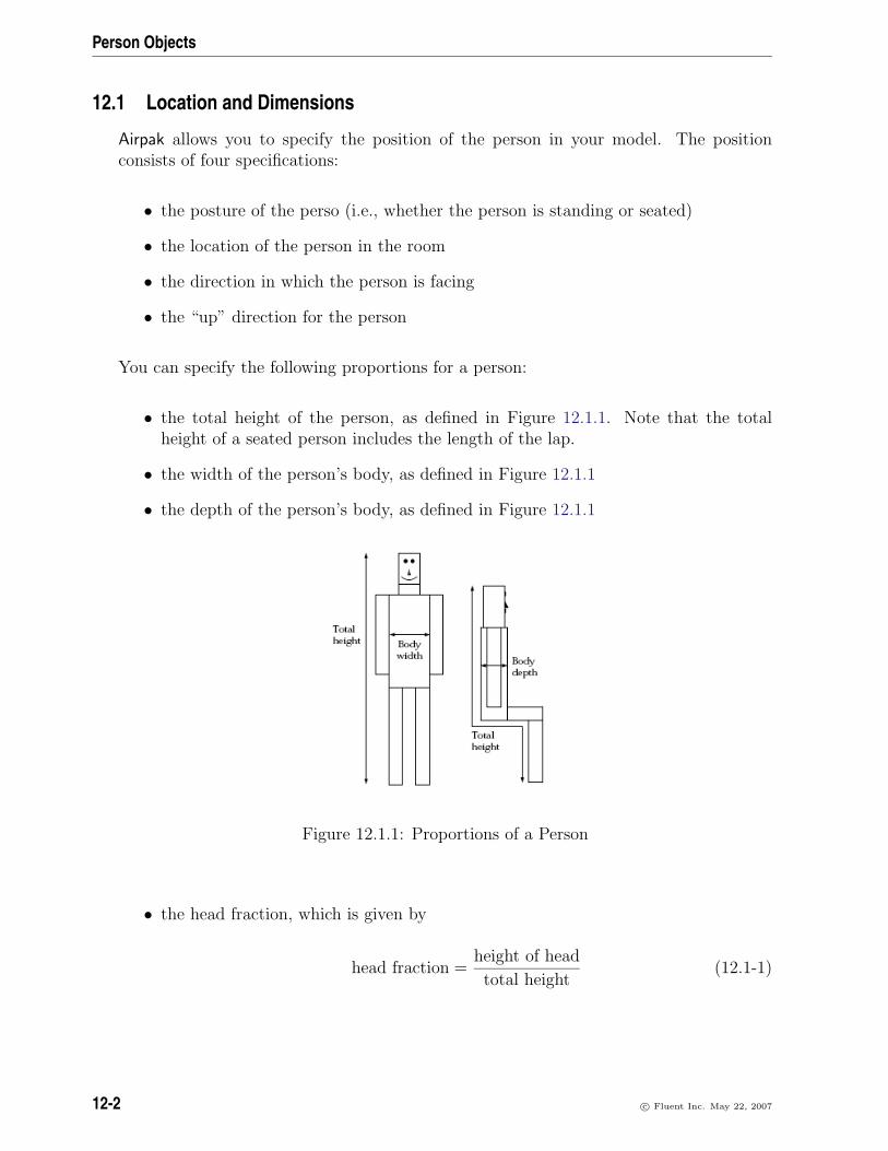
Person Objects
12.1 Location and Dimensions
Airpak allows you to specify the position of the person in your model. The positionconsists of four specifications:
• the posture of the perso (i.e., whether the person is standing or seated)
• the location of the person in the room
• the direction in which the person is facing
• the “up” direction for the person
You can specify the following proportions for a person:
• the total height of the person, as defined in Figure 12.1.1. Note that the totalheight of a seated person includes the length of the lap.
• the width of the person’s body, as defined in Figure 12.1.1
• the depth of the person’s body, as defined in Figure 12.1.1
Figure 12.1.1: Proportions of a Person
• the head fraction, which is given by
head fraction =height of head
total height(12.1-1)
12-2 c© Fluent Inc. May 22, 2007

12.2 Thermal Options
• the body fraction, which is given by
body fraction =height of body
total height(12.1-2)
• the lap fraction (if seated), which is given by
lap fraction =length of thigh
total height(12.1-3)
You can also specify the individual sizes of the following parts of a person’s body:
• head
• face
• body
• arms
• legs (vertical part only, if seated)
• thighs (if seated)
12.2 Thermal Options
You can specify the thermal boundary conditions of a person using one of three options:
Heat/area sets the flux of heat per unit area of the person. This is the default thermalboundary condition for the person, and the default value is 1 met (1 metabolic rateunit = 58.2 W/m2).
Total heat sets the total power output of the person.
Temperature sets the fixed value of the person’s temperature.
12.3 Adding a Person to Your Airpak Model
To include a person in your Airpak model, click on the button in the Object cre-
ation toolbar and then click on the button to open the Persons panel, shown inFigure 12.3.1.
c© Fluent Inc. May 22, 2007 12-3

Person Objects
Figure 12.3.1: The Person Panel
12-4 c© Fluent Inc. May 22, 2007

12.3 Adding a Person to Your Airpak Model
The procedure for adding a person to your Airpak model is as follows:
1. Create a person. See Section 7.3.2 for details on creating a new object and Sec-tion 7.3.9 for details on copying an existing object.
2. Change the description of the person, if required. See Section 7.4.1 for details.
3. Change the graphical style of the person, if required. See Section 7.4.2 for details.Note that you can turn off the display of the person’s face by deselecting theDecoration option for the person in the Graphical styles panel (see Section 6.3.6 fordetails about using the Graphical styles panel).
4. Specify the position of the person in the room. (See also Section 7.3.7 for detailson repositioning an object.)
(a) Select whether the person is Standing or Seated.
(b) Select the Up direction for the person. The up direction is the direction of thevector from the person’s feet to the person’s head.
(c) Select the direction in which the person is facing next to Facing direction. Youcan also specify whether the person is facing Forward or Backward. If youspecify that the person is facing Forward, they will face toward the positivedirection of the axis selected next to Facing direction.
(d) Specify the Location of the person in the model.
5. Specify the size of the person. (See also Section 7.3.6 for details on resizing anobject.) You can specify the size of the person in two ways: by specifying therelative proportions of the person, or by specifying the sizes of the individual partsof the body.
• To specify the relative proportions of the person:
(a) Make sure that Fix shapes is selected.
(b) Specify the Total height of the person. Note that for a seated person, thisheight includes the length of the lap.
(c) Specify the Body width and Body depth of the person.
(d) Specify the Head fraction, which is the height of the head as a fraction ofthe total height.
(e) Specify the Body fraction, which is the height of the body as a fraction ofthe total height.
(f) Specify the Lap fraction (if the person is seated), which is the length ofthe thighs as a fraction of the total height.
• To specify the sizes of the individual parts of the body:
c© Fluent Inc. May 22, 2007 12-5

Person Objects
Figure 12.3.2: The Person shape data Panel
(a) Deselect Fix shapes and click Edit details to open the Person shape datapanel (Figure 12.3.2).
(b) Select one of the body parts under Section.
(c) Keep the default Origin of (0, 0, 0), or specify the Origin for the body part(if required).
(d) Select Start/end and enter values for the start coordinates (xS, yS, zS) andend coordinates (xE, yE, zE) of the body part, or select Start/length andenter values for the start coordinates (xS, yS, zS) and lengths of the sides(xL, yL, and zL) of the body part.
Note that the left thigh (L.thigh) and right thigh (R.thigh) are specifiedas None if the person is standing. If you want to specify a thigh for astanding person, select Default and specify the starting and ending points(or the starting point and the lengths of the sides) for the thigh.
Note that the face is rectangular and not a prism like the other bodyparts. Specify the plane in which the face lies (Y-Z, X-Z, or X-Y). SelectStart/end and enter values for the start coordinates (xS, yS, zS) and endcoordinates (xE, yE, zE) of the face, or select Start/length and enter valuesfor the start coordinates (xS, yS, zS) and lengths of the sides (xL, yL, andzL) of the face.
(e) Click Done to save the changes to the person and close the Person shapedata panel.
6. Specify the thermal conditions of the person in the Person panel. There are threeoptions:
12-6 c© Fluent Inc. May 22, 2007

12.3 Adding a Person to Your Airpak Model
Heat/area allows you to enter the flux of heat per unit area of the person.
Total heat allows you to enter a value for the total heat output of the person.
Temperature allows you to specify the fixed value of the person’s temperature.
7. Specify the surface material (Surf material) to be used for the person. This materialdefines the roughness and emissivity of the person. By default, the surface materialis specified as Skin-Clothed. To change the surface material, select a material fromthe Surf material drop-down list. The surface roughness parameters and emissivityare defined as part of the surface material parameters. You can edit these values ifyou select Edit definition in the materials list. See Section 7.7 for details on materialproperties.
8. Select Radiation if the person is subject to radiative heat transfer. This option isavailable if you have selected On next to Radiation in the Problem setup panel andyou have not selected the Discrete ordinates radiation model option. You can modifythe default radiation characteristics of the person (e.g., view factor) by using theRadiation specification panel. To open this panel, select Radiation in the Personpanel and then click Edit. See Chapter 22 for details on radiation modeling.
c© Fluent Inc. May 22, 2007 12-7

Person Objects
12-8 c© Fluent Inc. May 22, 2007

Chapter 13. Walls
Walls are objects that constitute all or part of the room boundary. Walls can be spec-ified with respect to their thickness, velocity, and heat flux. Wall geometries includerectangular, 2D polygon, circular, and inclined.
By default, the room sides are zero-thickness walls with zero velocity and zero heat fluxboundary conditions. To modify the characteristics of the room boundaries, you mustcreate and specify thermal conditions on external walls. To construct a wall internal tothe enclosure, you must specify a thickness for the wall. The inner surface of an externalwall is in direct contact with the enclosure fluid, and its outer surface is exposed tothe external environment. A no-slip velocity boundary condition is applied at the innersurface of the wall. For turbulent flows, you can also specify the surface roughness of thewall, the effect of which is to increase resistance to the flow.
Throughout this section, reference will be made to the inside and outside of a wall. Theinside of the wall is the side in contact with the fluid in the room; the outside of thewall is the side exposed to the conditions external to the room. For a wall with zerothickness, the inner and outer sides of the wall coincide; however, the inner and outersurface materials can be different.
To configure a wall in the model, you must specify its geometry (including location anddimensions), velocity, thickness, thermal characteristics, and the material the wall ismade from.
In this chapter, information about the characteristics of a wall is presented in the followingsections:
• Section 13.1: Geometry, Location, and Dimensions
• Section 13.2: Surface Roughness
• Section 13.3: Wall Velocity
• Section 13.4: Thermal Boundary Conditions
• Section 13.5: External Thermal Conditions
• Section 13.6: Constructing Multifaceted Walls
• Section 13.7: Adding a Wall to Your Airpak Model
c© Fluent Inc. May 22, 2007 13-1

Walls
13.1 Geometry, Location, and Dimensions
Wall location and dimension parameters vary according to the wall geometry. Wallgeometries include rectangular, 2D polygon, circular, and inclined. These geometries aredescribed in Section 7.4.4.
13.1.1 Wall Thickness
For walls with non-zero thickness, Airpak automatically extends the wall inward or out-ward from the specified plane of the wall. The direction of this extension is determinedby the sign of the specified thickness relative to the coordinate axis normal to the plane ofthe wall. If the thickness value is positive, then the expansion is in the positive directionof the coordinate axis normal to the wall, as shown in Figure 13.1.1. If the thicknessvalue is negative, the expansion is in the negative direction.
− Thickness
+ Thickness
Plane of the wall
X
Y
Z
Figure 13.1.1: Wall Thickness Direction
Walls with non-zero thickness can conduct heat either through or along the plane of thewall, and can do so anisotropically, i.e., according to thermal conductivities specific toeach direction (defined as part of the properties of the solid material specified for thewall). They must possess a physical thickness so that Airpak can mesh the interior ofthe wall. Effective-thickness walls have the same properties as non-zero-thickness walls,except that they have no physical thickness; they can possess only an effective thickness.
13-2 c© Fluent Inc. May 22, 2007

13.2 Surface Roughness
13.2 Surface Roughness
In fluid dynamics calculations, it is common practice to assume that boundary surfacesare perfectly smooth. In laminar flow, this assumption is valid, because the length scalesof typical rough surfaces are much smaller than the length scales of the flow. In turbulentflow, however, the length scales of the flow eddies are much smaller than laminar lengthscales; therefore, it is sometimes necessary to account for surface roughness. Surfaceroughness acts to increase resistance to flow, leading to higher rates of heat transfer.
Airpak assumes, by default, that all surfaces of a wall in contact with a fluid are hydrody-namically smooth, and applies standard no-slip boundary conditions. For turbulent-flowsimulations in which roughness is significant, however, you can specify a roughness factorfor the entire wall. This roughness factor is defined as part of the properties of the surfacematerial specified for the wall. The purpose of the roughness factor is to approximatethe average height of the surface texture on the wall.
13.3 Wall Velocity
In most cases, walls represent stationary objects, but occasionally circumstances arisein which the model requires walls that move. For example, if the moving belt shown inFigure 13.3.1 is located at the room boundary, it can be represented as a wall moving ata fixed velocity. Moving walls always have zero thickness.
Z
Y
X
A V B
Actual
A BModelMoving wall
V
Figure 13.3.1: Moving Walls
c© Fluent Inc. May 22, 2007 13-3

Walls
When a wall is specified as moving, it is allowed to move only in the plane of the wall,i.e., there is no translation of the wall outside its plane. Also, fluid in contact with thewall is pulled along with the wall because of the no-slip condition. In such cases, thevelocity of the wall relative to the stationary enclosure must be set in the plane of thewall. For the example shown in Figure 13.3.1, the wall must be specified with a velocityof V in the x direction and zero velocity in the y direction. Airpak automatically imposesa velocity of zero in the direction normal to the plane of the wall (the z direction in thisexample).
13.4 Thermal Boundary Conditions
External walls can have two distinct thermal boundary conditions: a specified heat flux ora fixed temperature. In both cases, the wall is assumed to have zero thickness by default.When neither parameter is known, the external wall can model conditions applied to theouter side of the wall that enable Airpak to compute the heat flux and the temperatureon the inside of the wall, as shown in Figure 13.4.1.
Externalambientconditions
Computedflow andthermal conditions
Enclosure
Figure 13.4.1: Thermal Boundary Conditions
13.4.1 Specified Heat Flux
The simplest thermal boundary condition for a wall is that of a specified heat flux. Inthis case, the amount of heat that can pass through the wall is specified as a constantvalue or as a spatial boundary profile, expressed as power per unit area (heat flux). Foran adiabatic wall, the heat flux is zero. For walls with non-zero thickness, the heat fluxis applied on the outer surface of the wall, as shown in Figure 13.4.2. An example of theuse of this capability might be modeling solar loading. For transient problems, you canspecify the variation of heat flux with time.
13-4 c© Fluent Inc. May 22, 2007

13.4 Thermal Boundary Conditions
Specified heat flux ortemperature appliedto a zero-thickness wall
Specified heat fluxor temperatureapplied to a thickwall
Figure 13.4.2: Specified Heat Flux or Specified Temperature
13.4.2 Specified Temperature
In most cases, the temperature at the inside surface of a wall is unknown. However, ifthe temperature is known (e.g., if the wall abuts some material or object whose absolutetemperature is known or easily determined), the temperature can be directly applied asthe thermal boundary condition at the inside surface of the wall, either as a constant valueor as a spatial boundary profile. For walls with non-zero thickness, the temperature isapplied on the outer surface of the wall, as shown in Figure 13.4.2. For transient problems,you can specify the variation of temperature with time.
c© Fluent Inc. May 22, 2007 13-5

Walls
13.5 External Thermal Conditions
In some situations, neither the heat flux nor the temperature on the inner side of theexternal wall is known. In this case, the external wall and the heat transfer from thesurface of the wall to the external environment can be modeled as a wall with a specifiedthickness. Alternatively, a zero-thickness wall can be specified with a convective and/orradiative heat transfer condition applied directly to the wall.
To compute heat transfer through a wall with non-zero thickness to the external en-vironment, the energy equation is used. For these calculations, you must specify theconductivity of the wall (k, defined as part of the properties of the solid material spec-ified for the wall) and the wall thickness (see Figure 13.5.1). For transient problems,you must also specify the density and specific heat of the wall (defined as part of theproperties of the solid material specified for the wall).
External wall
Enclosure
Ambient temperatureT
Convective heatloss or gain
Specified heattransfer coefficient, h
Wall has specified thickness and conductivity, k
c
ambient
Figure 13.5.1: Wall with Non-Zero Thickness
Heat can also be lost or gained through the outside surface of an external wall by con-vective heat transfer and radiative heat transfer. The inner surface of an external wallcan also convect heat or radiate to objects within the room. These two types of heattransfer conditions can be applied to walls with either zero or non-zero thickness.
13.5.1 Convective Heat Transfer
The convective heat transfer boundary condition can be written as
qconv = hc(Twall − Tambient) (13.5-1)
where qconv is the heat gain or loss, hc is the heat transfer coefficient, Twall is the computedwall temperature, and Tambient is the external specified ambient temperature, i.e., the
13-6 c© Fluent Inc. May 22, 2007

13.5 External Thermal Conditions
temperature of the external fluid. From Equation 13.5-1, if the wall temperature isgreater than the ambient temperature, an amount of heat proportional to the temperaturedifference is lost to the environment from the room. Similarly, if the wall temperature islower than the external temperature, heat is transferred into the room. In contrast, thespecified heat flux option prescribes a specified heat gain or loss at the wall independentof the wall or ambient temperatures.
The heat transfer coefficient can be specified as a constant value, as a spatial profile, oras a function of temperature. For transient problems, you can specify the variation ofthe heat transfer coefficient with time.
In circumstances where heat transfer through the wall is not required (e.g., if the wall isthin and made of a highly conducting material), the thickness of the wall can be set tozero. In this case, the convective heat transfer boundary condition is applied directly tothe inside surface of the external wall.
13.5.2 Radiative Heat Transfer
The radiative heat transfer boundary condition provides for heat transfer between theroom wall and a remote surface. It can be written as
qrad = eσF (T 4wall − T 4
remote) (13.5-2)
where qrad is the heat gain or loss due to radiation (i.e., the net radiant flux from thewall surface), Tremote is the temperature of the remote surface, σ is the Stefan-Boltzmannconstant, F is a view factor specifying the fraction of radiant energy that is interceptedby the wall, and e is the surface emissivity of the wall (defined as part of the propertiesof the surface material specified for the wall). An example of the use of this capabilitymight be a room within a room whose walls are at a constant temperature, as shownin Figure 13.5.2. In this case, the room walls exchange radiant energy with the remotesurfaces.
In circumstances where heat transfer through the wall is not required (e.g., if the wall isthin and made of a highly conducting material), the thickness of the wall can be set tozero. In this case the radiative heat transfer boundary condition is applied directly tothe inside surface of the external wall.
c© Fluent Inc. May 22, 2007 13-7

Walls
Figure 13.5.2: Radiative Heat Transfer
13-8 c© Fluent Inc. May 22, 2007

13.6 Constructing Multifaceted Walls
13.6 Constructing Multifaceted Walls
When an adiabatic block is used to change the shape or size of a room, or to mask aportion of the room to be excluded from the computational domain, the sides of the blockrepresent enclosure boundaries. You can position an external wall on one or more of theblock surfaces, as shown in Figure 13.6.1. The main reason for using a wall in this wayis that an external wall might provide better control of heat transfer behavior than thesurface of a block.
EnclosureExternalwalls
Blocked-out volume
Figure 13.6.1: Blocked-Out Volumes
It is not necessary to separate an external wall into sections in order to accommodatevents, openings, or fans. Airpak automatically removes the wall definition from the spaceoccupied by the vents, openings, or fans; in effect, it cuts the appropriately sized holesin the wall to accommodate these objects, as shown in Figure 13.6.2.
Vent
External wall
Fan
Figure 13.6.2: Wall with Overlaid Objects
This same approach can be used to construct walls that are made up of different materials.Consider the example shown in Figure 13.6.3, where a wall is composed of two differentmaterials: Wall 1 is made of Material 1 and Wall 2 is made of Material 2. Wall 1 shouldbe created first, then Wall 2. The second wall definition will override the first when Wall2 is overlaid on Wall 1, effectively cutting a comparably-sized area out of Wall 1 andsubstituting Wall 2 into the hole.
c© Fluent Inc. May 22, 2007 13-9

Walls
Wall 1 Material 1
Wall 2
Material 2
Figure 13.6.3: Multifaceted Walls
13.7 Adding a Wall to Your Airpak Model
To include a wall in your Airpak model, click on the button in the Object creation
toolbar and then click on the button to open the Walls panel, shown in Figures 13.7.1and 13.7.2.
The procedure for adding a wall to your Airpak model is as follows:
1. Create a wall. See Section 7.3.2 for details on creating a new object and Section 7.3.9for details on copying an existing object.
2. Change the description of the wall, if required. See Section 7.4.1 for details.
3. Change the graphical style of the wall, if required. See Section 7.4.2 for details.
4. In the Geometry tab, specify the geometry, position, and size of the wall. There arethree different kinds of geometry available for walls in the Shape drop-down list.The inputs for these geometries are described in Section 7.4.4. See Section 7.3.6for details on resizing an object and Section 7.3.7 for details on repositioning anobject.
5. In the Properties tab, specify the type of the wall by selecting Stationary, Symmetry,or Moving next to Wall type. The lower part of the panel will change depending onyour selection of the Wall type.
6. Specify the characteristics related to the selected Wall type. These options aredescribed below.
13-10 c© Fluent Inc. May 22, 2007

13.7 Adding a Wall to Your Airpak Model
Figure 13.7.1: The Walls Panel (Geometry Tab)
c© Fluent Inc. May 22, 2007 13-11
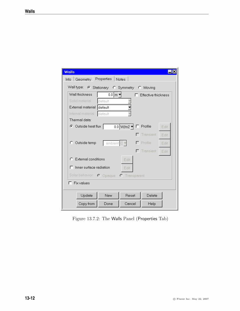
Walls
Figure 13.7.2: The Walls Panel (Properties Tab)
13-12 c© Fluent Inc. May 22, 2007

13.7 Adding a Wall to Your Airpak Model
13.7.1 User Inputs for a Symmetry Wall
The velocity component normal to a symmetry wall is set to zero. This option allowsyou to model half of a room in the case where the room is geometrically symmetric abouta center plane. When the Symmetry option is selected, you cannot specify any thermaldata and Airpak automatically specifies a zero heat flux condition at the symmetry plane.
There are no additional inputs for a symmetry wall.
13.7.2 User Inputs for a Stationary or Moving Wall
To specify a stationary wall or a moving wall, select Stationary or Moving next to Walltype in the Walls panel. The user inputs for a stationary wall are shown below. The userinputs for a moving wall are almost identical to those for a stationary wall, except thatthe motion of the wall must also be specified.
The steps for defining a stationary wall or a moving wall are as follows:
1. Select Stationary or Moving to specify whether the wall is stationary or moving. Fora stationary wall, the flow velocity is zero at the wall.
2. (stationary wall only) Specify the Wall thickness. When the wall thickness is non-zero, the heat flow through the wall is computed based on the conductivity of the
c© Fluent Inc. May 22, 2007 13-13

Walls
wall, the computed inner wall temperature on the inner surface of the wall, and theconditions applied at the outer surface of the wall.
If the thickness is non-zero, the wall is expanded inward or outward from theplane of the wall. If the thickness is positive, the wall is expanded to the specifiedthickness in the positive direction of the coordinate axis that is normal to the planeof the wall. If the thickness is specified with a negative sign, the expansion is inthe negative direction of the coordinate axis normal to the plane of the wall.
3. (stationary rectangular walls only) Select the Effective thickness option if you wantthe specified Wall thickness to be only an effective thickness.
4. (stationary wall only) If you specify a non-zero thickness for the wall, you mustalso specify the Solid material for the wall. By default, this is specified as defaultfor the wall. This means that the material specified as the Solid material for thewall is defined under Default solid in the Basic parameters panel (see Section 6.4.7).To change the Solid material for the wall, select a material from the Solid materialdrop-down list. See Section 7.7 for details on material properties.
5. Specify the External material for the wall. By default, this is specified as default forthe wall. This means that the material specified as the External material for the wallis defined under Default surface in the Basic parameters panel (see Section 6.4.7).To change the External material for the wall, select a material from the Externalmaterial drop-down list. The surface roughness and emissivity are defined as partof the surface material parameters. You can edit these values if you select Editdefinition in the materials list. See Section 7.7 for details on material properties.
6. If you specify a non-zero thickness for a stationary wall, or if you select a movingwall, you can specify the Internal material for the wall. By default, this is specifiedas default for the wall. This means that the material specified as the Internalmaterial for the wall is defined under Default surface in the Basic parameters panel(see Section 6.4.7). To change the Internal material for the wall, select a materialfrom the Internal material drop-down list. The surface roughness and emissivity aredefined as part of the surface material parameters. You can edit these values if youselect Edit definition in the materials list. See Section 7.7 for details on materialproperties.
i For a zero-thickness wall, changing the External material does not automat-ically change the Internal material. In these cases, the Internal material willbe set to the default surface material unless you have changed the Internalmaterial prior to specifying the zero-thickness wall.
7. (moving wall only) Set the Velocity vector (X, Y, Z) for the movement of the wall.Only the components of velocity in the plane of the wall can be set to non-zerovalues. The component of velocity normal to the wall is automatically set to zero.
13-14 c© Fluent Inc. May 22, 2007

13.7 Adding a Wall to Your Airpak Model
8. Specify the Thermal data for the wall. There are three options:
• Specify the Outside heat flux for the wall. To specify a uniform fixed rateof heat transfer through the wall, enter a value in the Outside heat flux textentry box. To define a spatial profile for the rate of heat transfer through thewall, select Profile next to Outside heat flux and click Edit to open the Curvespecification panel (described below).
If you are setting up a transient simulation, you can specify the Outside heatflux as a function of time. This option is available if you have selected Transientunder Time variation in the Basic parameters panel. To edit the transientparameters for the heat flux, select Transient and click Edit in the Walls panel.See Chapter 20 for more details on transient simulations.
i Note that Airpak cannot use both a spatial profile and a transient profilefor the outside heat flux. If you specify both profile types, Airpak will usethe transient profile and ignore the spatial profile.
• Specify the Outside temp of the wall. To specify a uniform fixed temperatureon the outer surface of the wall, enter a value in the Outside temp text entrybox. To define a spatial profile for the temperature on the outer surface ofthe wall, select Profile next to Outside temp and click Edit to open the Curvespecification panel (described below).
If you are setting up a transient simulation, you can specify the Outside temp asa function of time. This option is available if you have selected Transient underTime variation in the Basic parameters panel. To edit the transient parametersfor the outside temperature, select Transient and click Edit in the Walls panel.See Chapter 20 for more details on transient simulations.
i Note that Airpak cannot use both a spatial profile and a transient profilefor the outside temperature. If you specify both profile types, Airpak willuse the transient profile and ignore the spatial profile.
• Specify the External conditions for the wall. The External conditions optionallows you to account for heat loss or gain at the outer surface of the wallthrough convective or radiative heat transfer. To specify the external condi-tions for the wall, select External conditions and click Edit. Airpak will openthe Wall external thermal conditions panel (Figure 13.7.3).
(a) To activate convective heat transfer at the outer surface of the wall, selectEnabled in the Wall external thermal conditions panel. To specify a uniformheat transfer coefficient, enter the value of the heat transfer coefficient (hc inEquation 13.5-1) in the Base value text entry field and select the Constant valueoption (default). To define a spatial profile for the heat transfer coefficient,select the Spatial profile option and click Edit to open the Curve specificationpanel (described below). To define a heat transfer coefficient that varies as a
c© Fluent Inc. May 22, 2007 13-15

Walls
Figure 13.7.3: The Wall external thermal conditions Panel
function of temperature, select the Temp dependent option and click Edit toopen the Curve specification panel (described below). You can also define theheat transfer coefficient as a function of temperature difference (relative to theambient temperature). To define a heat transfer coefficient that varies as afunction of temperature difference, select dT dependent and click Edit to openthe Curve specification panel (described below).
The heat transfer coefficient can also be set automatically using existingempirical Nusselt correlations for forced convection and natural convectionflows. These correlations depend on the geometry of the wall, fluid prop-erties, Reynolds number (for forced convection flows), and Rayleigh number(for natural convection flows). To specify the heat transfer coefficient usingcorrelations select the Use correlations option and click Edit to open the Flowdependent heat transfer panel (Figure 13.7.4).
13-16 c© Fluent Inc. May 22, 2007
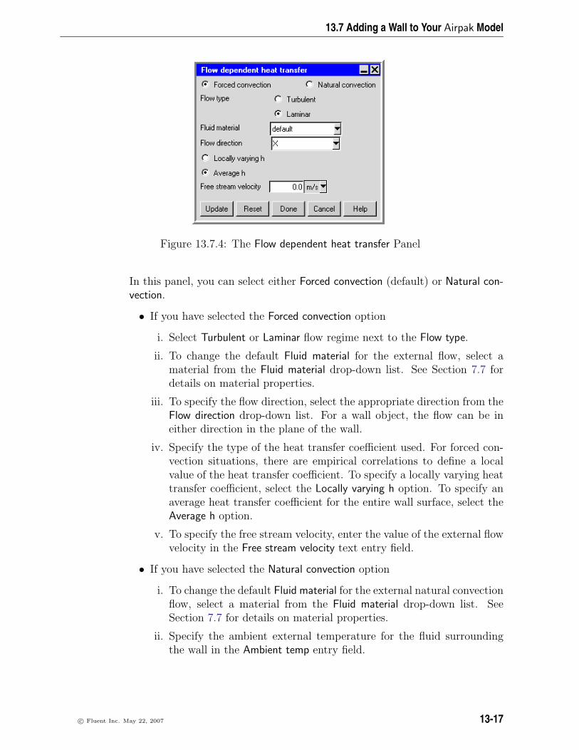
13.7 Adding a Wall to Your Airpak Model
Figure 13.7.4: The Flow dependent heat transfer Panel
In this panel, you can select either Forced convection (default) or Natural con-vection.
• If you have selected the Forced convection option
i. Select Turbulent or Laminar flow regime next to the Flow type.
ii. To change the default Fluid material for the external flow, select amaterial from the Fluid material drop-down list. See Section 7.7 fordetails on material properties.
iii. To specify the flow direction, select the appropriate direction from theFlow direction drop-down list. For a wall object, the flow can be ineither direction in the plane of the wall.
iv. Specify the type of the heat transfer coefficient used. For forced con-vection situations, there are empirical correlations to define a localvalue of the heat transfer coefficient. To specify a locally varying heattransfer coefficient, select the Locally varying h option. To specify anaverage heat transfer coefficient for the entire wall surface, select theAverage h option.
v. To specify the free stream velocity, enter the value of the external flowvelocity in the Free stream velocity text entry field.
• If you have selected the Natural convection option
i. To change the default Fluid material for the external natural convectionflow, select a material from the Fluid material drop-down list. SeeSection 7.7 for details on material properties.
ii. Specify the ambient external temperature for the fluid surroundingthe wall in the Ambient temp entry field.
c© Fluent Inc. May 22, 2007 13-17

Walls
iii. Specify the orientation of the surface with respect to gravity. Theheat transfer coefficients for natural convection flow depend on theorientation of the wall surface relative to the direction of gravity. Tospecify the orientation of the surface, select one of the following threeoptions under Surface: Vertical, Top, and Bottom.
For example, if gravity is in the negative Y direction, the XY and Y Zplanes are the Vertical surfaces, the high XZ plane is the Top surface,and the low XZ plane is the Bottom surface. To specify the directionof the gravity, select the appropriate axis from the Gravity directiondrop-down list.
If you are setting up a transient simulation, you can specify the Heattrans coeff as a function of time. This option is available if you haveselected Transient under Time variation in the Basic parameters panel.To edit the transient parameters for the heat transfer coefficient, selectTransient and click Edit in the Wall external thermal conditions panel.See Chapter 20 for more details on transient simulations.
i Note that Airpak cannot use both a spatial profile and a tran-sient profile for the heat transfer coefficient. If you specify bothprofile types, Airpak will use the transient profile and ignore thespatial profile.
Specify the ambient external temperature (i.e., Tambient in Equation 13.5-1)next to Ambient temp for the convective heat transfer boundary condi-tion. The value of the ambient temperature is defined under Ambientvalues in the Basic parameters panel (see Section 6.4.6).
(b) To activate radiative exchange of heat between the exterior surface of thewall and a remote surface, select Outer surface radiation in the Wall externalthermal conditions panel. Then specify the following parameters: Referencetemp (Tremote in Equation 13.5-2) and View factor. The value of the ambienttemperature is defined under Ambient values in the Basic parameters panel (seeSection 6.4.6).
If you are setting up a transient simulation, you can specify the reference tem-perature as a function of time. To define the variation of reference temperatureas a function of time, select Transient next to Reference temp, and click Edit.This will open the Transient temperature panel shown in Figure 20.1.6. Fordetails on specifying the transient temperature see Section 20.1.
View factor of the remote surface (i.e., the fraction of radiant energy that isintercepted by the wall). The default View factor is 1.0.
(c) Click Done in the Wall external thermal conditions panel to accept your changesand close the panel.
13-18 c© Fluent Inc. May 22, 2007

13.7 Adding a Wall to Your Airpak Model
9. (optional) Specify the radiative heat transfer parameters for the inner surface ofthe wall. This option is available if you have selected On next to Radiation in theBasic parameters panel. You can modify the default radiation characteristics of theinner surface of the wall (e.g., the view factor) by using the Radiation specificationpanel. To open this panel, select Inner surface radiation in the Walls panel and thenclick Edit. See Chapter 22 for details on radiation modeling.
Using the Curve specification Panel to Specify a Spatial Boundary Profile
You can define a spatial boundary profile using the Curve specification panel (Figure 13.7.5).To open the Curve specification panel, select Profile in the Walls panel or Spatial profile inthe Wall external thermal conditions panel, and click Edit.
You can also define the variation of the heat transfer coefficient with temperature ortemperature difference using the Curve specification panel. To open the Curve specificationpanel, select Temp dependent or dT dependent in the Wall external thermal conditions panel,and click Edit.
Figure 13.7.5: The Curve specification Panel
To define a spatial boundary profile, specify a list of (x, y, z) coordinates and the corre-sponding values in the Curve specification panel. For example, the first line in Figure 13.7.5specifies an outside heat flux of 1 W/m2 at (0.25, 0.25, 0). The data in Figure 13.7.5specify a variation of heat flux on the plane 0.25 ≤ x ≤ 0.75, 0.25 ≤ y ≤ 0.75, z = 0.The values in the right-hand column are the rate of heat transfer through the wall, thetemperature on the outer surface of the wall, or the heat transfer coefficient at the outersurface of the wall, depending on your selection under Thermal data in the Walls panel.
c© Fluent Inc. May 22, 2007 13-19

Walls
To define a temperature/heat transfer coefficient curve, specify a list of temperature/heattransfer coefficient pairs in the Curve specification panel. It is important to give thenumbers in pairs, but the spacing between numbers is not important.
Click Accept when you have finished defining the profile or curve; this will store the valuesand close the Curve specification panel. Airpak will interpolate the data you provide inthe Curve specification panel to create a profile for the whole boundary.
i If the starting point of the wall object is located at (x0,y0,z0), then the first pointof the profile should be (x0 y0 z0 a0), where a0 is the corresponding value for thatpoint. However, if the first point in the profile has a different value, for example (x1
y1 z1 a0), Airpak will automatically translate the first point to (x0 y0 z0 a0), and therest of the profile points will be shifted by (x1−x0,y1−y0,z1−z0). This translationof point locations will not affect the values of the variables (an), and is also usefulif the opening is ever translated within the model. In this way, you will not haveto recreate the profile file or re-enter values in the Curve specification panel. Thistranslation feature also applies to other objects that allow the specification of pointprofiles (i.e., openings, blocks, and resistances).
To load a previously defined profile or curve, click on Load. (See Section 28.2.8 fordetails on saving contour data and using them as a profile.) This will open the Loadcurve file selection dialog box. Select the file containing the profile or curve data andclick Accept. See Section 2.1.8 for details on selecting a file. If you know the units usedin the profile or curve data you are loading, you should select the appropriate units in theCurve specification panel before you load the profile or curve data. If you want to viewthe imported data after you have loaded it, using different units than the default unitsin the Curve specification panel, select the relevant Fix values options and then select theappropriate units from the unit definition lists.
If you want to load a curve file that you have created outside of Airpak, you will needto make sure that the first three lines of the file before the data contain the followinginformation:
1. the number of data sets in the file (usually 1)
2. the unit specifications for the file, which can be obtained from the Curve specificationpanel (e.g., units m W/m2)
3. the number of data points in the file (e.g., 5)
Using the above example, the first three lines of the curve file would be
1
units m W/m2
5
13-20 c© Fluent Inc. May 22, 2007

13.7 Adding a Wall to Your Airpak Model
The actual data points should be entered in the same was as you would enter them inthe Curve specification panel.
i If you want to load a curve from an Excel file, make sure that you also save thefile as formatted text (space delimited) before reading it into Airpak.
To save a profile or curve, click on Save. This will open the Save curve dialog box, inwhich you can specify the filename and directory to which the profile or curve data areto be saved.
c© Fluent Inc. May 22, 2007 13-21

Walls
13-22 c© Fluent Inc. May 22, 2007

Chapter 14. Partitions
Partitions are objects that are impervious to fluid flow. They can possess a thicknessand are defined by both their geometry and their type. Partition geometries includerectangular, 2D polygon, circular, inclined and 2D CAD.
Partition types are defined by their associated thermal models, including adiabatic thin,conducting thick, conducting thin, hollow thick, or contact resistance. Adiabatic thinpartitions do not conduct heat either across or in the plane of the partition. Conduct-ing thick partitions can conduct heat in either direction and they possess a thickness.Conducting thin partitions can conduct heat in either direction and have no physicalthickness. Hollow thick partitions can conduct heat in the plane of the partition but notacross the partition. Contact resistance partitions model resistances to heat transfer dueto barriers such as surface coatings or glues. Fluid partitions are also available and canbe used to cut a hole into a solid partition.
In this chapter, information about the characteristics of a partition is presented in thefollowing sections:
• Section 14.1: Defining a Partition in Airpak
• Section 14.2: Geometry, Location, and Dimensions
• Section 14.3: Thermal Model Type
• Section 14.4: Surface Roughness
• Section 14.5: Using Partitions in Combination with Other Objects
• Section 14.6: Adding a Partition to Your Airpak Model
c© Fluent Inc. May 22, 2007 14-1

Partitions
14.1 Defining a Partition in Airpak
In Airpak, partition sides are referred to as high and low, relative to the coordinates of theplane perpendicular to the partition (see Figure 14.1.1). The no-slip boundary conditionapplies at any partition surface in contact with the fluid and, for turbulent flows, youcan specify a surface roughness for each side of the partition. The sides of a partitioncan exchange radiation with other objects in the model.
Low sides
High sides
X
Y
Z
Figure 14.1.1: High/Low Side Partition Definition
To configure a partition in the model, you must specify its geometry (including locationand dimensions) and type, as well as the thermal characteristics, and the material fromwhich each side is made.
14.2 Geometry, Location, and Dimensions
The location and dimension parameters for a partition vary according to the geometryof the partition. Partition geometries include rectangular, 2D polygon, circular, inclinedand 2D CAD. These geometries are described in Section 7.4.4.
14.2.1 Partition Thickness
When a rectangular, 2D polygon, or circular partition is specified with a non-zero thick-ness, the thickness extends in either the positive or the negative coordinate direction(normal to the plane of the partition), depending on whether the thickness is specifiedas a positive or negative value. For an inclined partition, Airpak distributes the specifiedthickness in equal portions on both sides of the partition.
14-2 c© Fluent Inc. May 22, 2007

14.3 Thermal Model Type
14.3 Thermal Model Type
Partitions are defined according to their associated thermal models, which can be speci-fied as adiabatic thin, conducting thick, conducting thin, hollow thick, or contact resis-tance.
Adiabatic thin partitions have zero thickness and do not conduct heat in any direction,either normal to the partition or along the plane of the partition.
Conducting thick partitions can conduct heat either through or along the plane of thepartition and can do so anisotropically, i.e., according to thermal conductivities specificto each direction (defined as part of the properties of the solid material specified for thepartition). They must possess a physical thickness; the thickness must be physical sothat Airpak can mesh the interior of the partition. For transient simulations, you canspecify both density and specific heat for the partition (defined as part of the propertiesof the solid material specified for the partition), thereby imparting a thermal mass. If aconducting thick partition is specified without thermal mass, it can conduct heat but itcannot accumulate heat.
Conducting thin partitions have the same properties as conducting thick partitions, ex-cept that they have no physical thickness. They can possess only an effective thickness.
Contact resistance partitions represent barriers to heat transfer either between objects orbetween an object and the adjacent fluid. You can specify the resistance of the barrier interms of a thermal conductivity or a contact resistance. The thermal-conductivity-basedresistance is defined by the thermal conductivity (defined as part of the properties of thesolid material specified for the partition) and the partition thickness. The partition mustbe specified with a constant material conductivity; i.e., the conductivity must not be afunction of temperature. Contact resistance partitions can possess an effective thickness,in which case Airpak will not mesh the interior of the partition.
Hollow thick partitions represent three-dimensional regions of the model for which onlyside characteristics are important. Airpak does not mesh or solve for temperature or flowwithin regions bounded by the sides of a hollow partition.
c© Fluent Inc. May 22, 2007 14-3

Partitions
14.4 Surface Roughness
In fluid dynamics calculations, it is common practice to assume that boundary surfacesare perfectly smooth. In laminar flow, this assumption is valid, because the length scalesof typical rough surfaces are much smaller than the length scales of the flow. In turbulentflow, however, the length scales of the flow eddies are much smaller than laminar lengthscales; therefore, it is sometimes necessary to account for surface roughness. Surfaceroughness acts to increase resistance to flow, leading to higher rates of heat transfer.
Airpak assumes, by default, that all surfaces of a partition are hydrodynamically smooth,and applies standard no-slip boundary conditions. For turbulent-flow simulations inwhich roughness is significant, however, you can specify a roughness factor for the entirepartition or for each individual side of the partition. The roughness factor is definedas part of the properties of the surface material for the partition. The purpose of theroughness factor is to approximate the average height of the surface texture on thepartition.
14.5 Using Partitions in Combination with Other Objects
Partitions can be used alone or in conjunction with other modeling objects to createcomplex objects in order to perform sophisticated thermal simulations. For example,partitions and blocks can be used to build compartment, offices, or even railroad cars ofvarying complexity.
14.6 Adding a Partition to Your Airpak Model
To include a partition in your Airpak model, click on the button in the Object
creation toolbar and then click on the button to open the Partitions panel, shownin Figures 14.6.1 and 14.6.2.
The procedure for adding a partition to your Airpak model is as follows:
1. Create a partition. See Section 7.3.2 for details on creating a new object andSection 7.3.9 for details on copying an existing object.
2. Change the description of the partition, if required. See Section 7.4.1 for details.
3. Change the graphical style of the partition, if required. See Section 7.4.2 for details.
4. In the Geometry tab, specify the geometry, position, and size of the partition. Thereare four different kinds of geometry available for partitions in the Shape drop-downlist. The inputs for these geometries are described in Section 7.4.4. See Section 7.3.6for details on resizing an object and Section 7.3.7 for details on repositioning anobject.
14-4 c© Fluent Inc. May 22, 2007

14.6 Adding a Partition to Your Airpak Model
Figure 14.6.1: The Partitions Panel (Geometry Tab)
5. In the Properties tab, specify the thermal model for the partition by selecting Con-ducting thick, Hollow thick, Contact resistance, Conducting thin, Adiabatic thin, orFluid under Thermal model. The lower part of the panel will change depending onyour selection of the Thermal model.
6. Specify the characteristics related to the selected Thermal model. These options aredescribed below.
7. Specify the properties for the Low side and the High side of the partition. Theseoptions are described in Section 14.6.2.
8. (circular partitions only) Specify the speed of Rotation (rpm).
9. If you have enabled solar loading in the Basic parameters panel, specify the Solarbehavior for the partition. See Section 22.5 for details.
c© Fluent Inc. May 22, 2007 14-5

Partitions
Figure 14.6.2: The Partitions Panel (Properties Tab)
14-6 c© Fluent Inc. May 22, 2007

14.6 Adding a Partition to Your Airpak Model
14.6.1 User Inputs for the Thermal Model
Conducting Thick Partitions
To specify a conducting thick partition, select Conducting thick under Thermal model inthe Partitions panel. The user inputs for the Conducting thick thermal model are shownbelow.
The steps for defining a partition with a Conducting thick thermal model are as follows:
1. Specify the Thickness of the partition.
2. Specify the Solid material for the partition. By default, this is specified as defaultfor the partition. This means that the material specified as the Solid materialfor the partition is defined under Default solid in the Basic parameters panel (seeSection 6.4.7). To change the Solid material for the partition, select a material fromthe Solid material drop-down list. See Section 7.7 for details on material properties.
3. Specify the total power dissipated by the partition. There are three options forspecifying the total power:
Constant value allows you to specify a constant value of the Total power.
Temp dep allows you to specify heat as a function of temperature. This optionis not available if the Transient option is selected.
Click Edit next to Temp dep in the Partitions panel to open the Temperaturedependent power panel (Figure 14.6.3).
Specify a value for the constant C. The value in the equation shown in the panelis either the Total power or the power Per unit area/volume specified in thePartitions panel. Define the temperature range for which the function is validby entering values (in Kelvin) for Low T and High T. The value of the ambient
c© Fluent Inc. May 22, 2007 14-7

Partitions
Figure 14.6.3: The Temperature dependent power Panel
temperature is defined under Ambient values in the Basic parameters panel (seeSection 6.4.6). If the temperature exceeds the specified value of High T, thenthe power is given by substituting the value of High T into the equation atthe top of the Temperature dependent power panel. If the temperature fallsbelow the specified value of Low T, then the power is given by substitutingthe value of Low T into the equation at the top of the Temperature dependentpower panel.
Transient allows you to specify the total power as a function of time. This optionis available if you have selected Transient under Time variation in the Basicparameters panel. Select Transient under Total power and enter a value for theTotal power. To edit the transient parameters for the partition, click Edit nextto Transient. See Chapter 20 for more details on transient simulations.
Hollow Thick Partitions
To specify a hollow thick partition, select Hollow thick under Thermal model in the Parti-tions panel. The user inputs for the Hollow thick thermal model are shown below.
The steps for defining a partition with a Hollow thick thermal model are as follows:
14-8 c© Fluent Inc. May 22, 2007

14.6 Adding a Partition to Your Airpak Model
1. Specify the Thickness of the partition.
2. Specify the Total power dissipated by the partition.
Contact Resistance Partitions
To specify a contact resistance partition, select Contact resistance under Thermal model inthe Partitions panel. The user inputs for the Contact resistance thermal model are shownbelow.
The steps for defining a partition with a Contact resistance thermal model are as follows:
1. If you want to specify an additional resistance, select Additional resistance.You canspecify the resistance by selecting one of the following options from the drop-downlist and entering appropriate values:
Conductance allows you to specify a value for the Conductance. The inverse ofthis value will be used to calculate the contact resistance of the partition.
Thermal resistance allows you to specify a value for the Thermal resistance toheat transfer.
Thermal impedance allows you to specify a value for the Thermal impedance.Airpak computes the thermal resistance of the partition as Z/A where Z is thethermal impedance of the partition and A is the area of the partition.
Thickness allows you to specify a value for the Effective thickness of a specifiedSolid material. The values of the thickness and the thermal conductivity of thesolid material will be used to calculate the contact resistance of the partition.The resistance is computed as d/k, where d is the effective thickness of thepartition and k is the thermal conductivity of the solid material (defined aspart of the properties of the solid material specified for the partition).
c© Fluent Inc. May 22, 2007 14-9

Partitions
By default, the Solid material is specified as default for the partition. Thismeans that the material specified as the Solid material for the partition isdefined under Default solid in the Basic parameters panel (see Section 6.4.7).To change the Solid material for the partition, select a material from the Solidmaterial drop-down list. See Section 7.7 for details on material properties.
2. Enter a value for the Total power dissipated by the partition.
Conducting Thin Partitions
To specify a conducting thin partition, select Conducting thin under Thermal model in thePartitions panel. The user inputs for the Conducting thin thermal model are shown below.
The steps for defining a partition with a Conducting thin thermal model are as follows:
1. Specify the Effective thickness for the partition.
2. Specify the Solid material for the partition. By default, this is specified as defaultfor the partition. This means that the material specified as the Solid materialfor the partition is defined under Default solid in the Basic parameters panel (seeSection 6.4.7). To change the Solid material for the partition, select a material fromthe Solid material drop-down list. See Section 7.7 for details on material properties.
3. Specify the total power dissipated by the partition. There are two options forspecifying the total power:
Constant value allows you to specify a constant value of the Total power.
Temp dep allows you to specify the power as a linear function of temperature.Select Temp dep under Total power in the Partitions panel, and enter a valueof the Total power. Click Edit next to Temp dep to open the Temperaturedependent power panel (Figure 14.6.3) . Specify a value for the constant C.
14-10 c© Fluent Inc. May 22, 2007

14.6 Adding a Partition to Your Airpak Model
The value in the equation at the top of the Temperature dependent power panelis the Total power specified in the Partitions panel. Define the temperaturerange for which the function is valid by entering values (in Kelvin) for Low Tand High T. The value of the ambient temperature is defined under Ambientvalues in the Basic parameters panel (see Section 6.4.6). If the temperatureexceeds the specified value of High T, then the power is given by substitutingthe value of High T into the equation at the top of the Temperature dependentpower panel. If the temperature falls below the specified value of Low T, thenthe power is given by substituting the value of Low T into the equation at thetop of the Temperature dependent power panel. Click Update to update thethermal specification of the partition.
Adiabatic Thin Partitions
An adiabatic partition does not conduct heat in any direction, either normal to thepartition or along the plane of the partition.
To specify an adiabatic thin partition, select Adiabatic thin under Thermal model in thePartitions panel. There are no additional inputs for an adiabatic thin partition.
Fluid Partitions
To specify a fluid partition, select Fluid under Thermal model in the Partitions panel. Theonly input for this model is the Thickness of the partition.
Note that the Side specification options in the Partitions panel are not available with theFluid thermal model. A fluid partition can only be used to cut a hole into a solid partition,as shown in Figure 14.6.4.
Fluid plate
Solid plate
Figure 14.6.4: Using a Fluid Partition
14.6.2 User Inputs for the Low- and High-Side Properties of the Partition
Airpak allows you to specify different physical characteristics for each side of the partition.If you select Low side next to Side specification in the Partitions panel (Figure 14.6.2) and
c© Fluent Inc. May 22, 2007 14-11

Partitions
then click Edit, Airpak will open the Low side surface properties panel (Figure 14.6.5). Ifyou select High side and then click Edit, Airpak will open the High side surface propertiespanel, which is identical to the Low side surface properties panel.
Figure 14.6.5: The Low side surface properties Panel
To define the physical characteristics for the low side or the high side of the partition,follow the steps below.
1. Specify the surface Material to be used for the current side of the partition. Thismaterial defines the roughness and emissivity for this side of the partition. Bydefault, this is specified as default, which means that the material specified for theside of the partition is defined in the Basic parameters panel (see Section 6.4.7). Tochange the material for the current side of the partition, select a material from theMaterial drop-down list. See Section 7.7 for details on material properties.
2. (conducting thick or hollow thick partitions only) If you want to specify an addi-tional resistance to heat transfer for the current side of the partition, select Addi-tional resistance. You can specify the resistance by selecting one of the followingoptions from the drop-down list and entering appropriate values:
Conductance allows you to specify a value for the Conductance (= hA). Theinverse of this value will be used to calculate the additional resistance of thecurrent side of the partition.
Thermal resistance allows you to specify a value for the thermal resistance (Ther-mal resistance = 1
hA). This value will be used to calculate the additional resis-
tance of the current side of the partition.
14-12 c© Fluent Inc. May 22, 2007

14.6 Adding a Partition to Your Airpak Model
Thermal impedance allows you to specify a value for the Thermal impedance.Airpak computes the thermal resistance of the partition as Z/A where Z is thethermal impedance of the partition and A is the area of the partition.
Thickness allows you to specify a value for the Thickness of a specified Solidmaterial. The values of the thickness and the thermal conductivity of the solidmaterial will be used to calculate the additional resistance of the current sideof the partition.
3. If the side of the partition is subject to radiative heat transfer, select Radiation.You can modify the default radiation characteristics of the partition (e.g., the viewfactor). See Chapter 22 for details on radiation modeling.
c© Fluent Inc. May 22, 2007 14-13

Partitions
14-14 c© Fluent Inc. May 22, 2007

Chapter 15. Sources
Sources represent regions in the model within which heat flux originates. Source ge-ometries include prism, cylinder, ellipsoid, elliptical cylinder, rectangular, circular, 2Dpolygon, and inclined. Sources can be used to specify the primary field variable of tem-perature. For transient problems, you can also define a period during which the source isactive. Two-dimensional sources can exchange radiation with other objects in the model.
To configure a source in the model, you must specify its geometry (including location anddimensions) and temperature options. For a transient simulation, you must also specifyparameters related to the source coefficients.
In this chapter, information about the characteristics of a source is presented in thefollowing sections:
• Section 15.1: Geometry, Location, and Dimensions
• Section 15.2: Thermal Options
• Section 15.3: Source Usage
• Section 15.4: Adding a Source to Your Airpak Model
15.1 Geometry, Location, and Dimensions
Source location and dimension parameters vary according to source geometries. Sourcegeometries include rectangular, circular, 2D polygon, inclined, prism, cylinder, ellipsoid,and elliptical cylinder. These geometries are described in Section 7.4.4.
c© Fluent Inc. May 22, 2007 15-1
Sources
15.2 Thermal Options
Energy sources are specified using one of the following options: total heat, per unitarea/volume, fixed value, temperature dependent, or transient. These options are de-scribed below and in the section describing user inputs for heat source parameters. Notethat the variable s represents the input value in each text field.
Total heat sets the total power output over the plane or through the volume to thevalue s. Airpak then computes the source per-unit-area (or volume) value by divid-ing by the area of the plane or the volume of the 3D region.
Per unit area/volume sets the flux of heat per unit area of the source (positive) or sink(negative) or per unit volume of the volume to the value s.
Fixed value sets the temperature of the fluid on the plane to the value s.
Temperature dependent sets the flux of heat per unit area of the source (positive) orsink (negative) or per unit volume of the volume to the value
s+ CT (15.2-1)
where T is the temperature computed by Airpak, and C and s are user-specifiedvalues. Note that the Temperature dependent option for temperature sources is de-signed to model temperature-maintaining sources. For such sources, the coefficientC must be negative. A positive value for the coefficient C will result in runawaytemperatures.
15.3 Source Usage
Some general points regarding source usage are as follows:
• A volumetric source placed within a flow region can be regarded as a “transparent”object; i.e., the fluid flows through it. Its only effect is to add an appropriate sourceterm to one of the governing equations being solved.
• If a 2D source is suspended in a fluid, it takes on the properties of the fluid, but itdoes not allow any fluid flow to pass through it; i.e., it behaves like an impermeablewall element.
• In general, 2D flux sources should be placed on the surface of another object, suchas a wall, block, or partition.
15-2 c© Fluent Inc. May 22, 2007

15.4 Adding a Source to Your Airpak Model
15.4 Adding a Source to Your Airpak Model
To include a source in your Airpak model, click on the button in the Object cre-
ation toolbar and then click on the button to open the Sources panel, shown inFigures 15.4.1 and 15.4.2.
Figure 15.4.1: The Sources Panel (Geometry Tab)
The procedure for adding a source to your Airpak model is as follows:
1. Create a source. See Section 7.3.2 for details on creating a new object and Sec-tion 7.3.9 for details on copying an existing object.
2. Change the description of the source, if required. See Section 7.4.1 for details.
3. Change the graphical style of the source, if required. See Section 7.4.2 for details.
c© Fluent Inc. May 22, 2007 15-3

Sources
Figure 15.4.2: The Sources Panel (Properties Tab)
4. In the Geometry tab, specify the geometry, position, and size of the source. Thereare eight different kinds of geometry available for sources in the Shape drop-downlist. The inputs for these geometries are described in Section 7.4.4. See Section 7.3.6for details on resizing an object and Section 7.3.7 for details on repositioning anobject.
5. In the Properties tab, specify the Heat source parameters for the source. Theseoptions are described below.
6. Specify a source of species withing the computational domain, if required. You caninput the species concentrations for the source by using the Species concentrationspanel. To open this panel, select Species in the Sources panel and click Edit. SeeChapter 21 for details on modeling species transport.
15-4 c© Fluent Inc. May 22, 2007

15.4 Adding a Source to Your Airpak Model
7. (2D sources only) Select Radiation to specify radiation as an active mode of heattransfer to and from the source, if required. You can modify the default radiationcharacteristics of the source (e.g., the view factor) by using the Radiation specifica-tion panel. To open this panel, select Radiation and then click Edit. See Chapter 22for details on radiation modeling.
15.4.1 User Inputs for Heat Source Parameters
The following options are available for specifying heat source parameters in the Sourcespanel.
Total heat allows you to enter a value for the total heat output over the plane of a 2Dsource or through the volume of a 3D source.
Per unit allows you to specify:
• the flux of heat per unit volume of the source for a 3D source by entering avalue for the flux of heat per unit volume next to volume.
• the flux of heat per unit area of the source for a 2D source by entering a valuefor the flux of heat per unit area next to area.
Fixed value allows you to specify the temperature of the source. The value of theambient temperature is defined under Ambient values in the Basic parameters panel(see Section 6.4.6). This option is available only for 2D sources.
Transient allows you to specify the power as a function of time. This option is availableif you have selected Transient under Time variation in the Basic parameters panel.To edit the transient parameters for the source, click Edit next to Transient. SeeChapter 20 for more details on transient simulations.
Not temperature dependent specifies that the heat input is independent of tempera-ture.
Temperature dependent allows you to specify heat as a function of temperature. Thisoption is not available if the Transient option is selected. There are two options tospecify the temperature dependence of power: linear and piecewise linear. SelectTemperature dependent under Heat source parameters in the Sources panel. ClickEdit next to Temperature dependent to open the Temperature dependent power panel(Figure 15.4.3).
Choose either the linear option or the piecewise linear option. If you choose thelinear option specify a value for the constant C. The value in the equation shownin the panel is either the Total power or the power Per unit area/volume specifiedin the Sources panel. Define the temperature range for which the function is validby entering values (in Kelvin) for Low T and High T. The value of the ambient
c© Fluent Inc. May 22, 2007 15-5

Sources
Figure 15.4.3: The Temperature dependent power Panel
temperature is defined under Ambient values in the Basic parameters panel (seeSection ??). If the temperature exceeds the specified value of High T, then thepower is given by substituting the value of High T into the equation at the top ofthe Temperature dependent power panel. If the temperature falls below the specifiedvalue of Low T, then the power is given by substituting the value of Low T into theequation at the top of the Temperature dependent power panel.
If you select the Piecewise linear option, click Edit to open the Curve specificationpanel. To define the temperature dependence of power, specify a list of temper-atures and the corresponding power values in the curve specification panel. It isimportant to give the numbers in pairs, but the spacing between numbers is notimportant. Click Accept when you have finished defining the curve; this will storevalues and close the Curve specification panel. Airpak will interpolate the data youprovide in the Curve specification panel to create a profile for the entire range oftemperatures (Figure 15.4.4). If the temperature exceeds the highest temperaturespecified in the curve, then the power is given by specified power at the highest tem-perature. Similarly if the temperature drops below the lowest temperature specifiedin the curve, the power is given by specified power at the lowest temperature.
i Note that piecewise linear option is available only for 2D sources.
i Note that the values entered are actual total powers and not power per unitarea.
15-6 c© Fluent Inc. May 22, 2007

15.4 Adding a Source to Your Airpak Model
Figure 15.4.4: Curve specification panel
c© Fluent Inc. May 22, 2007 15-7

Sources
15-8 c© Fluent Inc. May 22, 2007

Chapter 16. Resistances
Resistances represent partial obstructions to flow within the room. Resistance geometriesinclude prism, cylinder, and 3D polygon. These types of resistances are three-dimensionaland represent flow resistance due to components such as wires, cables, and insulationmaterials packed within a portion of the room.
Rectangular, circular, inclined, and 2D polygon resistances are 2D shapes and are de-signed to model planar flow obstructions such as screens, vents, and permeable baffles.See Chapter 10 for more information on 2D resistances.
The effect of any resistance is modeled as a pressure drop through its area or volume.Alternatively, the pressure drop across the resistance can be calculated using either theapproach-velocity method or the device-velocity method, both of which require a user-specified velocity loss coefficient. The approach-velocity and device-velocity methodsdiffer from each other only by virtue of a factor called the free area ratio. The calculatedpressure drop can be proportional either to the fluid velocity itself, or to the square of thevelocity. It is common practice to employ the linear relationship for laminar flow and thequadratic relationship for turbulent flow. In the general case, a combination of the linearand quadratic relationships may more accurately model the pressure drop/volumetricflow curve. Airpak also provides a power-law method for calculating the pressure dropthrough a 3D resistance.
i Note that you cannot use the hexahedral mesher if a resistance is placed on aninclined conducting thick partition. The tetrahedral mesher, on the other hand,can be used with all types of resistances.
To configure a 3D resistance in the model, you must specify its geometry (including loca-tion and dimensions), the pressure drop model, and the relationship between resistanceand velocity. You must also specify the fluid material for the resistance and the totalpower dissipated by the resistance.
In this chapter, information about the characteristics of a 3D resistance is presented inthe following sections:
• Section 16.1: Geometry, Location, and Dimensions
• Section 16.2: Pressure Drop Calculation for a 3D Resistance
• Section 16.3: Adding a Resistance to Your Airpak Model
c© Fluent Inc. May 22, 2007 16-1

Resistances
16.1 Geometry, Location, and Dimensions
3D resistance location and dimension parameters vary according to resistance geometries.Resistance geometries include prism, cylinder, and 3D polygon. These geometries aredescribed in Section 7.4.4.
16.2 Pressure Drop Calculation for a 3D Resistance
For a 3D resistance, Airpak provides a power-law method for calculating the pressuredrop across the resistance:
∆p = Cvn (16.2-1)
where ∆p is the pressure drop across the 3D resistance, v is the velocity, and C and nare constants.
Alternatively, Airpak can calculate the pressure drop resulting from a resistance either bythe approach-velocity method or by the device-velocity method. Because the resistanceto the fluid flow due to a volumetric resistance may be different in each of the threecoordinate directions, you must provide the loss coefficient and the method to calculatethe pressure drop in each direction for a 3D resistance.
The approach-velocity method relates the pressure drop to the fluid velocity:
∆p = ρlc12vnapp (16.2-2)
where lc is the user-specified loss coefficient (for each coordinate direction in 3D), ρ is thefluid density, and vapp is the approach velocity. The approach velocity in Equation 16.2-2is the component of the approach velocity in the appropriate coordinate direction (x, y,or z) as computed by Airpak. The velocity dependence can be linear (n = 1), quadratic(n = 2), or a combination of linear and quadratic.
The device-velocity method relates the pressure drop induced by the resistance to thefluid velocity:
∆p = ρlc22vndev (16.2-3)
where vdev is the device velocity. The velocity dependence can be linear (n = 1), quadratic(n = 2), or a combination of linear and quadratic.
The difference between the approach-velocity and device-velocity methods is in the ve-locity used to compute the pressure drop. The device velocity is related to the approachvelocity by
16-2 c© Fluent Inc. May 22, 2007

16.2 Pressure Drop Calculation for a 3D Resistance
vdev =vapp
A(16.2-4)
where A is the free area ratio. The free area ratio is the ratio of the area through whichthe fluid can flow unobstructed to the total planar area of the obstruction.
i Note that the loss coefficient used in the equation for the device velocity is notthe same as the loss coefficient used in the equation for the approach velocity. Theloss coefficients in Equations 16.2-2 and 16.2-3 are related to the flow regime of theproblem:
• For a viscous flow regime (e.g., laminar flow, slow flow, very dense packing), youshould select a linear velocity relationship:
∆p =ρ
2lc1v (16.2-5)
• For an inertial flow regime (e.g., turbulent flow), you should select a quadraticvelocity relationship:
∆p =ρ
2lc2v
2 (16.2-6)
• For a combination of these two types of flow, you should select a linear+quadraticvelocity relationship:
∆p = ∆plinear + ∆pquadratic (16.2-7)
You can obtain the loss coefficients in several ways:
• experimental measurements
• computational measurements
• from a reference (The loss coefficients for many vent configurations are available in[14].)
c© Fluent Inc. May 22, 2007 16-3

Resistances
16.3 Adding a Resistance to Your Airpak Model
To include a resistance in your Airpak model, click on the button in the Object
creation toolbar and then click on the button to open the Resistances panel, shownin Figures 16.3.1 and 16.3.2.
Figure 16.3.1: The Resistances Panel (Geometry Tab)
The procedure for adding a resistance to your Airpak model is as follows:
1. Create a resistance. See Section 7.3.2 for details on creating a new object andSection 7.3.9 for details on copying an existing object.
2. Change the description of the resistance, if required. See Section 7.4.1 for details.
3. Change the graphical style of the resistance, if required. See Section 7.4.2 fordetails.
16-4 c© Fluent Inc. May 22, 2007
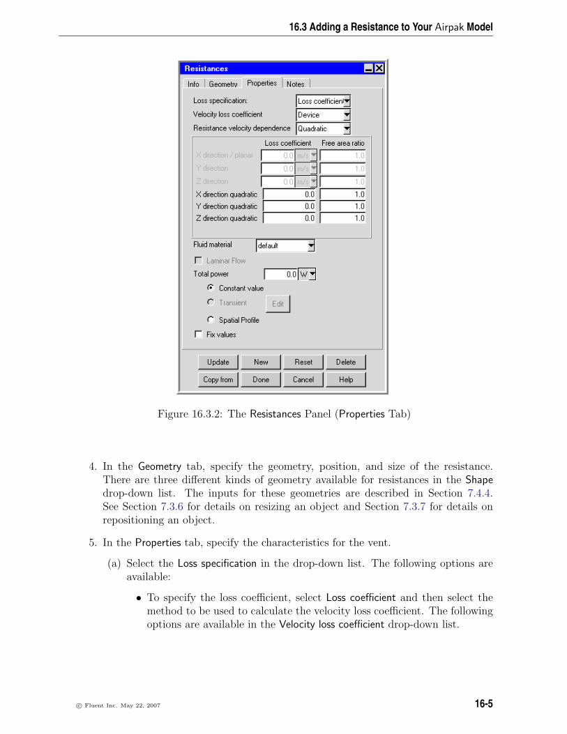
16.3 Adding a Resistance to Your Airpak Model
Figure 16.3.2: The Resistances Panel (Properties Tab)
4. In the Geometry tab, specify the geometry, position, and size of the resistance.There are three different kinds of geometry available for resistances in the Shapedrop-down list. The inputs for these geometries are described in Section 7.4.4.See Section 7.3.6 for details on resizing an object and Section 7.3.7 for details onrepositioning an object.
5. In the Properties tab, specify the characteristics for the vent.
(a) Select the Loss specification in the drop-down list. The following options areavailable:
• To specify the loss coefficient, select Loss coefficient and then select themethod to be used to calculate the velocity loss coefficient. The followingoptions are available in the Velocity loss coefficient drop-down list.
c© Fluent Inc. May 22, 2007 16-5
Resistances
– To use the device-velocity method, select Device and select the methodto be used to calculate the Resistance velocity dependence. Thereare three options in the drop-down list: Linear, Quadratic, and Lin-ear+quadratic. Finally, specify the linear and/or quadratic Loss coef-ficient and Free area ratio for each of the three coordinate directions.
– To use the approach-velocity method, select Approach and select themethod to be used to calculate the Resistance velocity dependence.Finally, specify the linear and/or quadratic Loss coefficient for each ofthe three coordinate directions.
– To calculate the pressure drop using a power-law method, select Powerlaw. Specify the Coefficient (C in Equation 16.2-1) and the Exponent(n in Equation 16.2-1).
i You must specify these inputs in SI units.
• To define a piecewise-linear profile for the pressure drop as a functionof the speed of the fluid through the resistance in the three coordinatedirections, select Loss curve. Airpak allows you to describe the curve(s)either by positioning a series of points on a graph using the Resistancecurve graphics display and control window, or by specifying a list of resis-tance speed/pressure coordinate pairs using the Curve specification panel.These options are available in the Edit drop-down lists for the X-direction,Y-direction, and Z-direction under Pressure loss curve data. For detailsabout using the Resistance curve and Curve specification panels, see Sec-tions 10.5.1 and 10.5.2.
To load a previously defined curve, click the appropriate Load button.This will open the Load curve file selection dialog box. Select the filecontaining the curve data and click Accept. See Section 2.1.8 for detailson selecting a file.
To save a curve, click the appropriate Save button. This will open theSave curve dialog box, in which you can specify the filename and directoryto which the curve data is to be saved.
i Note that the boxes to the right of the Edit drop-down lists will beempty if you have not defined a curve for the resistance in a particulardirection. Each box will contain the first speed value if you havedefined a curve for that direction.
(b) Specify the Fluid material for the resistance. By default, this is specified asdefault for the resistance. This means that the material specified as the Fluidmaterial for the resistance is defined under Default fluid in the Basic parameterspanel (see Section 6.4.7). To change the Fluid material for the resistance, selecta material from the Fluid material drop-down list. See Section 7.7 for detailson material properties.
16-6 c© Fluent Inc. May 22, 2007
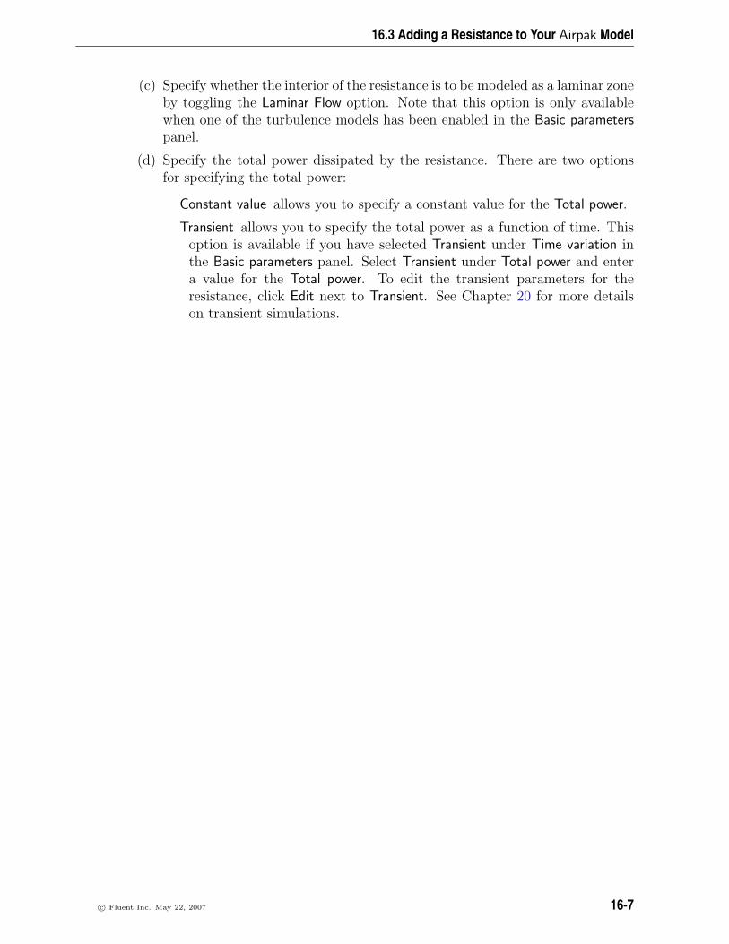
16.3 Adding a Resistance to Your Airpak Model
(c) Specify whether the interior of the resistance is to be modeled as a laminar zoneby toggling the Laminar Flow option. Note that this option is only availablewhen one of the turbulence models has been enabled in the Basic parameterspanel.
(d) Specify the total power dissipated by the resistance. There are two optionsfor specifying the total power:
Constant value allows you to specify a constant value for the Total power.
Transient allows you to specify the total power as a function of time. Thisoption is available if you have selected Transient under Time variation inthe Basic parameters panel. Select Transient under Total power and entera value for the Total power. To edit the transient parameters for theresistance, click Edit next to Transient. See Chapter 20 for more detailson transient simulations.
c© Fluent Inc. May 22, 2007 16-7

Resistances
16-8 c© Fluent Inc. May 22, 2007

Chapter 17. Heat Exchangers
Heat exchangers are two-dimensional modeling objects representing the heat exchangewith the surrounding air. For a planar heat exchanger in Airpak, a lumped-parametermodel is used to model a heat exchange element. The heat exchanger allows you tospecify both the pressure drop and heat transfer coefficient as functions of the velocitynormal to the radiator.
In this chapter, information about the characteristics of heat exchangers is presented inthe following sections:
• Section 17.1: Geometry, Locations, and Dimensions
• Section 17.2: Modeling a Planar Heat Exchanger in Airpak
• Section 17.3: Adding a Heat Exchanger to Your Airpak Model
17.1 Geometry, Location, and Dimensions
Heat exchanger location and dimension parameters vary according to the geometry. Heatexchanger geometries include rectangular, inclined, circular, and 2D polygon. Thesegeometries are described in Section 7.4.4.
17.2 Modeling a Planar Heat Exchanger in Airpak
A lumped-parameter model for a heat exchange element (for example, a radiator orcondenser), is available in Airpak. The heat exchanger allows you to specify both thepressure drop and the heat transfer coefficient as functions of the velocity normal to theheat exchanger.
17.2.1 Modeling the Pressure Loss Through a Heat Exchanger
In the heat exchanger model in Airpak, the heat exchanger is considered to be infinitelythin, and the pressure drop through the heat exchanger is assumed to be proportional tothe dynamic head of the fluid, with an empirically determined loss coefficient which yousupply. That is, the pressure drop, ∆p, varies with the normal component of velocitythrough the radiator, v, as follows:
∆p = kL1
2ρv2 (17.2-1)
c© Fluent Inc. May 22, 2007 17-1

Heat Exchangers
where ρ is the fluid density, and kL is the non-dimensional loss coefficient, which can bespecified as a constant or as a polynomial function.
In the case of a polynomial, the relationship is of the form
kL =N∑n=1
rnvn−1 (17.2-2)
where rn are polynomial coefficients and v is the magnitude of the local fluid velocitynormal to the resistance.
17.2.2 Modeling the Heat Transfer Through a Heat Exchanger
The heat flux from the heat exchanger to the surrounding fluid is given as
q = h(Tair,d − Text) (17.2-3)
where q is the heat flux, Tair,d is the temperature downstream of the heat exchanger, andText is the reference temperature for the liquid. The convective heat transfer coefficient,h, can be specified as a constant or as a polynomial function.
For a polynomial, the relationship is of the form
h =N∑n=0
hnvn; 0 ≤ N ≤ 7 (17.2-4)
where hn are polynomial coefficients and v is the magnitude of the local fluid velocitynormal to the resistance in m/s.
Either the actual heat flux (q) or the heat transfer coefficient and heat exchanger tem-perature (h, Tair,d) may be specified. q (either the entered value or the value calculatedusing Equation 17.2-3) is integrated over the heat exchanger surface area.
17.2.3 Calculating the Heat Transfer Coefficient
To model the thermal behavior of the heat exchanger, you must supply an expression forthe heat transfer coefficient, h, as a function of the fluid velocity through the resistance,v. To obtain this expression, consider the heat balance equation:
q =mcp∆T
A= h(Tair,d − Text) (17.2-5)
where
17-2 c© Fluent Inc. May 22, 2007

17.3 Adding a Heat Exchanger to Your Airpak Model
q = heat fluxm = fluid mass flow ratecp = specific heat capacity of fluidh = empirical heat transfer coefficientText = external temperature (reference temperature for the liquid)Tair,d = temperature downstream from the heat exchangerA = heat exchanger frontal area
Equation 17.2-5 can be rewritten as
q =mcp(Tair,u − Tair,d)
A= h(Tair,d − Text) (17.2-6)
where Tair,u is the upstream air temperature. The heat transfer coefficient, h, can there-fore be computed as
h =mcp(Tair,u − Tair,d)
A(Tair,d − Text)(17.2-7)
or, in terms of the fluid velocity,
h =ρvcp(Tair,u − Tair,d)
Tair,d − Text
(17.2-8)
17.3 Adding a Heat Exchanger to Your Airpak Model
To include a heat exchanger in your Airpak model, click on the button in the Object
creation toolbar and then click on the button to open the Heat exchangers panel,shown in Figures 17.3.1 and 17.3.2.
The procedure for adding a heat exchanger to your Airpak model is as follows:
1. Create a heat exchanger. See Section 7.3.2 for details on creating a new object andSection 7.3.9 for details on copying an existing object.
2. Change the description of the heat exchanger, if required. See Section 7.4.1 fordetails.
3. Change the graphical style of the heat exchanger, if required. See Section 7.4.2 fordetails.
4. In the Geometry tab, specify the geometry, position, and size of the heat exchanger.There are four different kinds of geometry available for heat exchangers in the Shapedrop-down list. The inputs for these geometries are described in Section 7.4.4.
c© Fluent Inc. May 22, 2007 17-3

Heat Exchangers
Figure 17.3.1: The Heat exchangers Panel (Geometry Tab)
Figure 17.3.2: The Heat exchangers Panel (Properties Tab)
17-4 c© Fluent Inc. May 22, 2007

17.3 Adding a Heat Exchanger to Your Airpak Model
See Section 7.3.6 for details on resizing an object and Section 7.3.7 for details onrepositioning an object.
5. In the Properties tab, specify the Loss coefficient for the heat exchanger. To specifya constant loss coefficient, select Constant and enter the value in the Constant textentry box. To specify a polynomial loss coefficient, select Polynomial and enter thecoefficients for the polynomial equation (separated by spaces) in the Polynomial textentry box. For example, if you have a polynomial equation of the form
a+ bv + cv2 + dv3
you would enter
a b c d
in the Polynomial text entry box.
i Note that you must use SI units for the polynomial equation.
6. Specify the Heat transfer through the heat exchanger. There are two options:
Heat flux specifies a fixed rate of heat transfer from the resistance to the sur-rounding fluid.
Heat tr coeff specifies a heat transfer coefficient to model the heat input/outputof the resistance. You can specify a Constant value for the heat transfer coeffi-cient (h in Equation 17.2-3). Alternatively, you can specify a Polynomial heattransfer coefficient by entering the coefficients for the polynomial equation(separated by spaces) in the Polynomial text entry field.
i Note that you must use SI units for the polynomial equation.
Specify the temperature of the resistance (i.e., Tair,d in Equation 17.2-3) nextto Extern temp. The value of the ambient temperature is defined under Ambientvalues in the Basic parameters panel (see Section 6.4.6).
c© Fluent Inc. May 22, 2007 17-5

Heat Exchangers
17-6 c© Fluent Inc. May 22, 2007

Chapter 18. Hoods
A hood is a three-dimensional modeling object that consists of a neck, a canopy, a flange,and exhausts. An example of a hood is shown in Figure 18.0.1.
Figure 18.0.1: An Example of a Hood
To configure a hood in the model, you must specify its location and dimensions. Youmust also specify the flow rate associated with the hood.
In this chapter, information about the characteristics of a hood is presented in the fol-lowing sections:
• Section 18.1: Location and Dimensions
• Section 18.2: Flow Rate
• Section 18.3: Adding a Hood to Your Airpak Model
18.1 Location and Dimensions
Airpak allows you to specify the position and size of the neck and canopy of the hood.You can also specify the position and size of the exhausts. The hood can have one ortwo exhausts: Airpak creates two exhausts by default.
You can select whether the flange is vertical (Figure 18.1.1) or horizontal (Figure 18.1.2)on the hood, or you can specify a hood without a flange. If the hood has a flange, youcan specify the height of the flange, or you can specify the sizes of its individual parts.
c© Fluent Inc. May 22, 2007 18-1

Hoods
Figure 18.1.1: Hood with Vertical Flange
Figure 18.1.2: Hood with Horizontal Flange
18-2 c© Fluent Inc. May 22, 2007

18.2 Flow Rate
18.2 Flow Rate
In Airpak, the flow rate for the hood can be specified in terms of total mass flow rate ortotal volume flow rate. If the hood has two exhausts of equal size, Airpak will divide thetotal mass (or volume) flow rate equally between the two exhausts. If the hood has twoexhausts of unequal sizes, Airpak will divide the total mass (or volume) flow rate betweenthe two exhausts based on the following equations:
m1 =A1
A1 + A2
× m (18.2-1)
m2 =A2
A1 + A2
× m (18.2-2)
where m1 is the mass (or volume) flow rate for exhaust 1, m2 is the mass (or volume)flow rate for exhaust 2, A1 is the area of exhaust 1, A2 is the area of exhaust 2, and mis the total mass (or volume) flow rate.
18.3 Adding a Hood to Your Airpak Model
To include a hood in your Airpak model, click on the button in the Object creation
toolbar and then click on the button to open the Hoods panel, shown in Figure 18.3.1.
The procedure for adding a hood to your Airpak model is as follows:
1. Create a hood. See Section 7.3.2 for details on creating a new object and Sec-tion 7.3.9 for details on copying an existing object.
2. Change the description of the hood, if required. See Section 7.4.1 for details.
3. Change the graphical style of the hood, if required. See Section 7.4.2 for details.
4. Specify the position of the hood in the room (see also Section 7.3.7 for details onrepositioning an object) and the overall size of the hood (see also Section 7.3.6 fordetails on resizing an object). You can specify the size and position of the hood inthe Properties tab in two ways:
• To specify the location and dimensions of one or more parts of the hood andhave Airpak adjust the relative location and dimensions of the other parts ofthe hood:
(a) Make sure that Fix shapes is selected in the Properties tab.
(b) If desired, specify the start coordinates (xS, yS, zS) and end coordinates(xE, yE, zE) of the Neck of the hood.
c© Fluent Inc. May 22, 2007 18-3

Hoods
Figure 18.3.1: The Hoods Panel (Properties Tab)
18-4 c© Fluent Inc. May 22, 2007

18.3 Adding a Hood to Your Airpak Model
(c) If desired, specify the start coordinates (xS, yS, zS) and end coordinates(xE, yE, zE) of the Canopy of the hood.
(d) If desired, specify the Flange type. There are three options: Vertical,Horizontal, or None. If you select Vertical or Horizontal, you must alsospecify the Height of the flange.
(e) If desired, specify the number of exhausts in the hood by selecting ordeselecting Exhaust 1 or Exhaust 2. Specify the start coordinates (xS, zS)and end coordinates (xE, zE) of Exhaust 1 and Exhaust 2, as required.
• To specify the location and dimensions of the individual parts of the hood(without any automatic adjustment of the other parts):
(a) Deselect Fix shapes in the Properties tab and click Edit details to open theHoods shape data panel (Figure 18.3.2).
Figure 18.3.2: The Hoods shape data Panel (Neck Tab)
(b) Select one of the parts of the hood under Section by clicking on the ap-propriate tab.
(c) Keep the default Origin of (0, 0, 0) or specify the Origin for the part (ifrequired).
(d) To specify the neck in the hood, click the Neck tab (Figure 18.3.2). Se-lect Start/end and enter values for the start coordinates (xS, yS, zS) andend coordinates (xE, yE, zE) of the neck. Alternatively, you can selectStart/length and enter values for the start coordinates (xS, yS, zS) andlengths of the sides (xL, yL, and zL) of the neck.
(e) To specify the canopy in the hood, click the Canopy tab (Figure 18.3.3).The default canopy is defined as a non-uniform polygon. Specify the plane
c© Fluent Inc. May 22, 2007 18-5

Hoods
in which the base lies (Y-Z, X-Z, or X-Y), the Height, and the coordinatesof its vertices (low 1, low 2, low 3, low 4, high 1, high 2, high 3, high 4).You can add and remove vertices using the Add and Rem buttons.
Figure 18.3.3: The Hoods shape data Panel (Canopy Tab)
If you select None under Plane, the polygonal block will be constructedwith zero height and will take the shape of the base of the polygon.
If you require a canopy with a uniform polygonal shape, deselect Nonuni-form and specify the plane in which the base lies (Y-Z, X-Z, or X-Y), theHeight, and the coordinates of the vertices (vert 1, vert 2, vert 3, vert 4)on the base plane.
(f) For each flange you want to specify in the hood, click the appropriateFlange tab (e.g., Flange1).
Select the plane in which the part of the flange lies (Y-Z, X-Z, or X-Y)in the Plane drop-down list (Figure 18.3.4). Select Start/end and entervalues for the start coordinates (xS, yS, zS) and end coordinates (xE, yE,zE) of the part of the flange, or select Start/length and enter values for thestart coordinates (xS, yS, zS) and lengths of the sides (xL, yL, and zL) ofthe part of the flange.
(g) For each exhaust that you want to include in the hood, use the horizontalscroll bar and click the appropriate Exhaust tab (e.g., Exhaust1).
18-6 c© Fluent Inc. May 22, 2007

18.3 Adding a Hood to Your Airpak Model
Figure 18.3.4: The Hoods shape data Panel (Flange Tab)
Specify the plane in which the exhaust lies (Y-Z, X-Z, or X-Y) in the Planedrop-down list (Figure 18.3.5).
Select Start/end and enter values for the start coordinates (xS, yS, zS)and end coordinates (xE, yE, zE) of the exhaust, or select Start/length andenter values for the start coordinates (xS, yS, zS) and lengths of the sides(xL, yL, and zL) of the exhaust.
(h) Click Done to save the changes to the hood and close the Hoods shapedata panel.
5. Specify the Flow rate in the Hoods panel. You can specify a Volume flow rate or aMass flow rate.
c© Fluent Inc. May 22, 2007 18-7
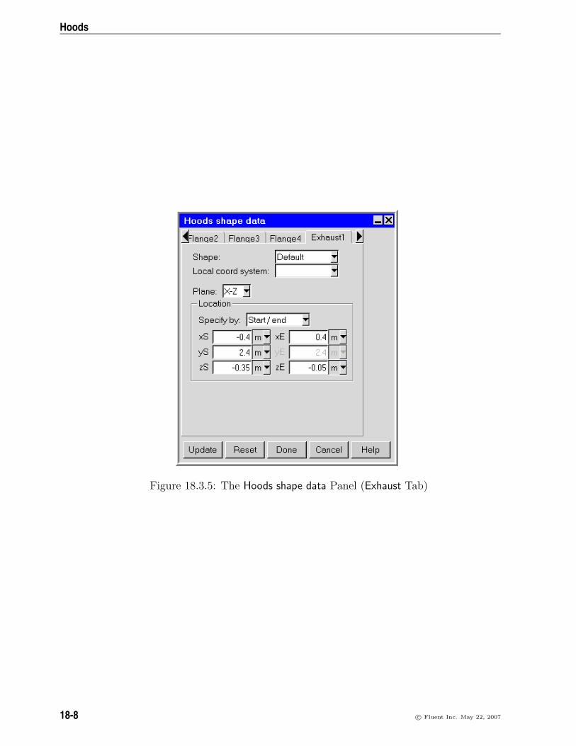
Hoods
Figure 18.3.5: The Hoods shape data Panel (Exhaust Tab)
18-8 c© Fluent Inc. May 22, 2007

Chapter 19. Wires
Wires are used to construct polygonal ducts of arbitrary cross-section. To construct aduct, a minimum of three wires are necessary. There is no upper limit to the number ofwires that can be used. Note that wires are not to be used by themselves; they are onlyused to construct polygonal ducts. To learn how to construct polygonal ducts, refer toSection 25.3.1.
To configure a wire in the model, the only parameters that you need to specify are thelocations of the vertices. A wire can have any number of vertices, and it need not beparallel to any axis.
i Polygonal duct macros created using wires must be meshed with the tetrahedralmesher. To learn how to use the tetrahedral mesher, refer to Section 26.3.
19.1 Adding a Wire to Your Airpak Model
To include a wire in your Airpak model, click on the button in the Object creation
toolbar and then click on the button to open the Wires panel, shown in Figure 19.1.1.
The procedure for adding a wire to your Airpak model is as follows:
1. Create a wire. See Section 7.3.2 for details on creating a new object and Sec-tion 7.3.9 for details on copying an existing object.
2. Change the description of the wire, if required. See Section 7.4.1 for details.
3. Change the graphical style of the wire, if required. See Section 7.4.2 for details.
4. Specify the vertices of the wire. There are two ways to modify the position of anyvertex on the wire:
• In the Geometry tab, select the name of the vertex (e.g., vert 1) in the vertexlist and modify its X, Y, and Z coordinate values.
• Use the <Shift> key and the right mouse button to move the vertex point inthe graphics window.
Use the Add and Rem buttons to add or delete vertices from the wire.
c© Fluent Inc. May 22, 2007 19-1

Wires
Figure 19.1.1: The Wires Panel (Geometry Tab)
19-2 c© Fluent Inc. May 22, 2007

Chapter 20. Transient Simulations
Airpak can solve the equations for conservation of mass, momentum, and energy in time-dependent form. Thus Airpak can be used to simulate a wide variety of time-dependentphenomena, including transient heat conduction and convection, as well as transientspecies tranport.
Activating time dependence is sometimes useful when attempting to solve steady-stateproblems that tend toward instability (e.g., natural convection problems in which theRayleigh number is close to the transition region). It is possible in many cases to reacha steady-state solution by integrating the time-dependent equations.
Airpak uses a fully-implicit time-integration scheme for transient analysis. This chapterprovides details about setting up a transient simulation in Airpak and postprocessing theresults. See Section 31.6.3 for details about the theory of transient simulations.
The information in this chapter is divided into the following sections:
• Section 20.1: User Inputs for Transient Simulations
• Section 20.2: Specifying Variables as a Function of Time
• Section 20.3: Postprocessing for Transient Simulations
20.1 User Inputs for Transient Simulations
To solve a transient problem, you will follow the procedure outlined below:
1. Enable the Transient option in the Transient setup tab of the Basic parameters panel(Figure 20.1.1). To open the Basic parameters panel, double-click on the Basicparameters item under the Problem setup node in the Model manager window.
Problem setup−→ Basic parameters
2. Enter the starting and ending times for the simulation in the Start and End entryfields.
3. To edit the default transient parameters (if required), click on Edit parameters. Thiswill open the Transient parameters panel shown in Figure 20.1.2.
c© Fluent Inc. May 22, 2007 20-1

Transient Simulations
Figure 20.1.1: The Basic parameters Panel (Transient setup Tab)
20-2 c© Fluent Inc. May 22, 2007

20.1 User Inputs for Transient Simulations
Figure 20.1.2: The Transient parameters Panel
c© Fluent Inc. May 22, 2007 20-3

Transient Simulations
(a) Specify a value for the Time step increment. The default value is 0.001 s.The specified Time step increment will be used for all time steps if Uniform isselected. It will also be used if Piecewise linear is selected and ts < t1 (seebelow).
(b) Specify the Solution save interval. This value tells Airpak how often during thesolution procedure the results should be saved. Every tenth time step is savedby default.
i Only steps that have been saved can be used during postprocessing.Large amounts of data can be generated from a transient simulation, soyou should decide how much data should be saved for postprocessing. Ifyou are only interested in the solution at the end of the transient simula-tion, then very little intermediate data need be saved. If you are interestedin animating and studying the transient effects in detail, then almost everytime step should be saved.
(c) Specify whether Airpak should use a uniform or non-uniform time step.
Uniform specifies a uniform time step. The value of the Time step incrementwill be used for all time steps.
Variable specifies a non-uniform time step. There are three options:
Linear (ts = i + a t) specifies a linear variation of the time step withtime:
∆t = ∆t0 + at (20.1-1)
where ∆t is the time step at time t, ∆t0 is the initial time step, anda is a constant. Enter values for the Initial step (i) and the Factor (a).
Square Wave specifies a square-wave profile for the time step variation.If the variation of time step required is regular/periodic with time,then this option can be used instead of the Piecewise constant option.To specify a square-wave profile, click Edit to open the Square WaveTime-Step Parameters panel (Figure 20.1.3).
To understand the meaning of the various parameters in the SquareWave Time-Step Parameters panel, see Figure 20.1.4.
Piecewise constant specifies a piecewise constant variation of the timestep. Enter a list of the time/time-step pairs in the Piecewise values(time / time-step) box at the bottom of the Transient parameters panel.It is important to give the numbers in pairs, but the spacing betweenthe numbers is not important. An example of the arrangement of thetime/time-step pairs is shown below:
20-4 c© Fluent Inc. May 22, 2007

20.1 User Inputs for Transient Simulations
Figure 20.1.3: The Square Wave Time-Step Parameters Panel
P: Phase delayDT : Max time step valueDT : Min time step valueT : Duration of DTT : Duration of DT
PDT
DT
T T
min
max
max
max
min
min
min
max
maxmin
Figure 20.1.4: The Square Wave Inputs for Time Step Variation
c© Fluent Inc. May 22, 2007 20-5

Transient Simulations
t1 ∆t1
t2 ∆t2
t3 ∆t3
Airpak will use the time/time-step pairs such that if t < t1, the timestep ∆t is given by
∆t = ∆t1 (20.1-2)
Similarly, if t1 ≤ t < t2,
∆t = ∆t2 (20.1-3)
Piecewise linear specifies a piecewise linear variation of the time step.Enter a list of the time/time-step pairs in the Piecewise values (time/ time-step) box at the bottom of the Transient parameters panel. Itis important to give the numbers in pairs, but the spacing betweenthe numbers is not important. An example of the arrangement of thetime/time-step pairs is shown below:
t1 ∆t1
t2 ∆t2
t3 ∆t3
Airpak will use the time/time-step pairs such that if ts < t ≤ t1, thetime step ∆t is a linear function that varies between ∆t0 and ∆t1:
∆t = ∆t0 +[∆t1 −∆t0t1 − ts
](t− ts) (20.1-4)
where ts is the Start time specified in the Basic parameters panel, and∆t0 is the Time step increment specified at the top of the Transientparameters panel.
Similarly, for t1 < t ≤ t2, ∆t is a linear function that varies between∆t1 and ∆t2:
∆t = ∆t1 +[∆t2 −∆t1t2 − t1
](t− t1) (20.1-5)
(d) Click Accept in the Transient parameters panel to store the new settings.
20-6 c© Fluent Inc. May 22, 2007

20.1 User Inputs for Transient Simulations
Figure 20.1.5: The Basic parameters Panel (Default values tab)
c© Fluent Inc. May 22, 2007 20-7

Transient Simulations
4. Specify an ambient value of temperature by entering the ambient Temperature underAmbient values in the Default values tab of the Basic parameters panel (Figure 20.1.5).
5. To define the variation of ambient temperature as a function of time, select Transientnext to Temperature, and then click Edit. This will open the Transient temperaturepanel shown in Figure 20.1.6.
i You must specify all inputs in SI units in the Transient temperature panel.
Figure 20.1.6: The Transient temperature Panel
(a) Select the method for the calculation of the variation of ambient temperaturewith time. The following options are available, and described in more detailin Section 20.2.
Linear specifies a linear variation of ambient temperature with time. Entera value for the coefficient a in Equation 20.2-1.
Power law specifies a power law variation of ambient temperature with time.Enter values for the coefficients a and b in Equation 20.2-2.
Exponential specifies an exponential variation of ambient temperature withtime. Enter a value for the coefficients a and b in Equation 20.2-3.
Sinusoidal specifies a sinusoidal variation of ambient temperature with time.Enter values for the period T , the phase shift t0, and the coefficient a inEquation 20.2-4.
20-8 c© Fluent Inc. May 22, 2007

20.1 User Inputs for Transient Simulations
Piecewise linear specifies a piecewise linear variation of ambient tempera-ture with time. There are two ways to define the piecewise linear vari-ation: the Time/value curve window and the Curve specification panel.These methods are described in Section 20.2.
Square wave specifies a square wave variation of ambient temperature withtime. Specify the Phase, the On time, the Off time, and the Off value forthe square wave, as described in Section 20.2.
(b) Click Done in the Transient temperature panel when you have finished specify-ing the variation of ambient temperature with time.
6. Specify the initial conditions for the fluid in your model in the Default values tabof the Basic parameters panel (Figure 20.1.5). For a transient simulation, thiscorresponds to the initial physical state of the fluid. See Section 6.4.8 for moredetails on setting initial conditions.
7. Once you have set the desired parameters in the Basic parameters panel, click Acceptto store the new settings.
8. Specify the transient characteristics of the objects in your Airpak model. You canspecify transient characteristics for the following objects:
• Solid or fluid block: Specify the total power as a function of time by selectingthe Transient option in the Properties tab of the Blocks panel (see Chapter 8)and clicking Edit. The Transient power panel used to define the transientpower of the block is very similar to the Transient temperature panel shown inFigure 20.1.6. You must also specify the start time tS and the end time tE forthe transient simulation for the block.
• Hollow block: Specify the species concentrations as a function of time (seeChapter 21 on species transport). Select Species in the Blocks panel and clickthe Edit button to open the Species concentrations panel. Select Transient forthe desired species and click Edit to open the Transient species panel. TheTransient species panel is used to define the transient species concentrationsfor the block and is very similar to the Transient temperature panel shown inFigure 20.1.6. You must also specify the start time tS and the end time tE forthe transient simulation for the block.
• Fan: Specify the transient strength of a characteristic curve fan by turningon Transient strength in the Properties tab of the Fans panel (see Chapter 9)and clicking Edit. The Transient fan strength panel used to define the transientstrength of the fan is similar to the Transient temperature panel shown inFigure 20.1.6, except that it contains only the Piecewise linear and Squarewave options.
• Vent: Specify the species concentrations as a function of time (see Chapter 21for information on species transport). Select Species in the Vents panel and
c© Fluent Inc. May 22, 2007 20-9

Transient Simulations
click the Edit button to open the Species concentration panel. Then follow theinstructions for the hollow block, described above.
• Opening: For a free opening, you can specify the static pressure, temper-ature, x velocity, y velocity, or z velocity for flow across the opening as afunction of time, by turning on the Transient option in the Properties tab ofthe Openings panel (see Chapter 11) and clicking Edit. The Transient pressure,Transient temperature, Transient X velocity, Transient Y velocity, and TransientZ velocity panels are very similar to the Transient temperature panel shown inFigure 20.1.6. You must also specify the start time tS and the end time tE forthe transient simulation for the opening.
i You must specify all inputs in SI units in the Transient temperaturepanel.
You can also specify the species concentrations as a function of time (see Chap-ter 21 for information on species transport). Select Species in the Openingspanel and click the Edit button to open the Species concentration panel. Thenfollow the instructions for the hollow block, described above.
For a recirculation opening, you can specify the start time (tS) and the endtime (tE) of the period when the opening is active.
• Wall: You can specify the rate of heat transfer through the wall or the tem-perature on the outer surface of the wall as a function of time, by turning onthe Transient option in the Properties tab of the Walls panel (see Chapter 11)and clicking Edit. You can also specify the heat transfer coefficient as a func-tion of time by turning on the Transient option in the Wall external thermalconditions panel. To open the Wall external thermal conditions panel, selectExternal conditions in the Walls panel and click Edit. The Transient power/area,Transient temperature, and Transient heat tr coeff panels are very similar to theTransient temperature panel shown in Figure 20.1.6. You must also specify thestart time tS and the end time tE for the transient simulation for the wall.
i You must specify all inputs in SI units in the Transient temperaturepanel.
• Conducting thick partition: Specify the total power as a function of time byselecting Transient in the Properties tab of the Partitions panel (see Chapter 14)and clicking Edit. The Transient power panel used to define the transient powerof the partition is very similar to the Transient temperature panel shown inFigure 20.1.6. You must also specify the start time tS and the end time tE forthe transient simulation for the partition.
• Source: Specify the power as a function of time by turning on the Transientoption in the Properties tab of the Sources panel (see Chapter 15) and clickingEdit. The Transient power panel used to define the transient power of the source
20-10 c© Fluent Inc. May 22, 2007

20.2 Specifying Variables as a Function of Time
is very similar to the Transient temperature panel shown in Figure 20.1.6. Youmust also specify the start time tS and the end time tE for the transientsimulation for the source.
You can also specify the species concentrations for a 2D source or the mass ofa species entering or leaving the room per second for a 3D source, as a functionof time (see Chapter 21 for information on species transport). Select Species inthe Sources panel and click the Edit button to open the Species concentrationspanel. Then follow the instructions for the hollow block, described above.
• Resistance: Specify the total power as a function of time by selecting Transientin the Properties tab of the Resistances panel (see Chapter 16) and clicking Edit.The Transient power panel used to define the transient power of the resistanceis very similar to the Transient temperature panel shown in Figure 20.1.6. Youmust also specify the start time tS and the end time tE for the transientsimulation for the resistance.
You can also specify the mass of a pecies entering or leaving the room per secondas a function of time (see Chapter 21 for information on species transport). Se-lect Species in the Resistances panel and click the Edit button to open the Speciesconcentrations panel. Then follow the instructions for the hollow block, describedabove.
i Note that the start time tS and the end time tE can be different for differentobjects.
9. Set the maximum number of iterations to be performed per time step underIterations/timestep in the Basic settings panel (Figure 20.1.7). To open this panel,double-click on the Basic settings item under the Solution settings node in the Modelmanager window. If the Convergence criteria are satisfied before this number of it-erations is performed, the solution will advance to the next time step. The defaultvalue of 20 iterations/time step should be acceptable for most cases. If you findthat the solution is not converging at each time step, you can increase the Itera-tions/timestep value and/or decrease the size of the Time step increment specifiedin the Transient parameters panel (Figure 20.1.2).
10. Start the calculation using the Solve panel. To open this panel, click Run solutionin the Solve menu. Click Start solution to start the calculation.
Files will be saved at the frequency specified next to Solution save interval in the Transientparameters panel (Figure 20.1.2). A separate file is saved for each time step for whichdata are saved.
20.2 Specifying Variables as a Function of Time
For transient simulations, you can specify variables that vary as a function of time.You can specify different kinds of variations, including linear, power law, exponential,
c© Fluent Inc. May 22, 2007 20-11

Transient Simulations
Figure 20.1.7: The Basic settings Panel for a Transient Simulation
sinusoidal, piecewise linear, and square wave:
• linear:
st = s0 + at (20.2-1)
where t is the time, st is the value of the variable at time t, s0 is the value of thevariable at t = 0, and a is a constant.
• power law:
st = s0 + atb (20.2-2)
where t is the time, st is the value of the variable at time t, s0 is the value of thevariable at t = 0, and a and b are constants.
• exponential:
st = s0 + beat (20.2-3)
where t is the time, st is the value of the variable at time t, s0 is the value of thevariable at t = 0, and a and b are constants.
• sinusoidal:
st = s0 + a sin[2π
T(t− t0)
](20.2-4)
20-12 c© Fluent Inc. May 22, 2007

20.2 Specifying Variables as a Function of Time
where t is the time, st is the value of the variable at time t, s0 is the value of thevariable at t = 0, T is the period, t0 is the phase shift, and a is a constant.
• piecewise linear:
st = s0f(t) (20.2-5)
where f(t) is a function of time, st is the value of the variable at time t, and s0 isthe value of the variable at t = 0. See Section 20.2.2 for information on definingf(t) using the Time/value curve window; see Section 20.2.3 for details on definingf(t) using the Curve specification panel.
• square wave:
st = s0f(t) (20.2-6)
where st is the value of the variable at time t and s0 is the value of the variable att = 0. f(t) is a function of time as shown in Figure 20.2.1.
0
On time
Off timePhasef(t)
t
Off value
Figure 20.2.1: Definition of a Square Wave
The Phase is the time between t = 0 and the first peak of the square wave. The Ontime is the time that the square wave is at its peak value. The Off time is the timebetween peak values of the square wave. The Off value is the value of the squarewaves between the peaks of the wave. The peak value is the specified value of thetransient quantity (e.g., 293 for Temperature in Figure 20.1.1).
20.2.1 Displaying the Variation of Transient Parameters with Time
After you have specified the transient parameters for your Airpak model (e.g., time step,temperature, power, etc.) you can display the variation of these parameters with timeusing the Transients panel (Figure 20.2.2). To open the Transients panel, click the Viewbutton under Time variation in the Transient setup tab of the Basic parameters panel.
The following functions are available for viewing the variation of transient parameters:
c© Fluent Inc. May 22, 2007 20-13

Transient Simulations
Figure 20.2.2: The Transients Panel
20-14 c© Fluent Inc. May 22, 2007

20.2 Specifying Variables as a Function of Time
• To display specified variation plots of the transient parameters as a function of time(e.g., time, ambient temp, power), toggle the check boxes in the upper left of thepanel .
• To update the variation plots after having made changes in the Basic parameterspanel, the Transient parameters panel, the Transient temperature panel, or any similartransient parameter panel, click Update.
• To display variation plots of all defined transient parameters, click Show all.
• To zoom into an area of the variation plot, click Zoom. Position the mouse pointerat a corner of the area to be zoomed, click the left mouse button, drag open aselection box to the desired size, and click the left button again. To cancel a zoombefore it is completed, click the right mouse button. To return to the default view,click Reset.
• To display the time-step points on the variation plots, turn on the Timesteps option.
• To non-dimensionalize the y axis of the variation plot; i.e., divide each parametervalue by the initial value of parameter, turn on the Nondimensional option.
20.2.2 Using the Time/value curve Window to Specify a Piecewise LinearVariation With Time
You can specify a piecewise linear variation of a variable with time using the Time/valuecurve graphics display and control window (Figure 20.2.3). To open the Time/value curvewindow, select Piecewise linear in the Transient temperature panel (Figure 20.1.6) or in anysimilar transient parameter panel, and click Edit. Select Graph editor from the resultinglist.
The following functions are available for creating, editing, and viewing a curve:
• To create a new point on the curve, click on the curve with the middle mousebutton.
• To move a point on the curve, hold down the middle mouse button while positionedover the point, and move the mouse to the new location of the point.
• To delete a point on the curve, click the right mouse button on the point.
• To zoom into an area of the curve, position the mouse pointer at a corner of thearea to be zoomed, hold down the left mouse button and drag open a selection boxto the desired size, and then release the mouse button. The selected area will thenfill the Time/value curve window, with appropriate changes to the axes. After youhave zoomed into an area of the model, click on Full range to restore the graph toits original axes and scale.
c© Fluent Inc. May 22, 2007 20-15

Transient Simulations
Figure 20.2.3: The Time/value curve Graphics Display and Control Window
20-16 c© Fluent Inc. May 22, 2007

20.2 Specifying Variables as a Function of Time
• To set the minimum and maximum values for the scales on the axes, click on Setrange. This will open the Set range panel (Figure 20.2.4).
Figure 20.2.4: The Set range Panel
Enter values for Min X, Min Y, Max X, and Max Y and click Accept.
• To load a previously defined curve, click on Load. This will open the Load curvefile selection dialog box. Select the file containing the curve data and click Accept.See Section 2.1.8 for details on selecting a file.
• To save a curve, click on Save. This will open the Save curve dialog box, in whichyou can specify the filename and directory to which the curve data is to be saved.
You can use the Print button to print the curve. See Section 3.5 for details on savinghardcopy files.
Click Done when you have finished creating the curve; this will store the curve and closethe Time/value curve graphics display and control window. Once the curve is defined,you can view the pairs of coordinates defining the curve in the Curve specification panel.See Figure 20.2.5 for the pairs of coordinates for the curve shown in Figure 20.2.3.
20.2.3 Using the Curve specification Panel to Specify a Piecewise LinearVariation With Time
You can define a piecewise linear variation of a variable with time using the Curve specifi-cation panel (Figure 20.2.5). To open the Curve specification panel, select Piecewise linearin the Transient temperature panel (Figure 20.1.6) or in any similar transient parameterpanel, and click Edit. Select Text editor from the resulting list.
To define a curve, specify a list of coordinate pairs in the Curve specification panel.It is important to give the numbers in pairs, but the spacing between numbers is notimportant. Click Accept when you have finished entering the pairs of coordinates; thiswill store the values and close the Curve specification panel.
Once the pairs of coordinates have been entered, you can view the piecewise linear curvein the Time/value curve graphics display and control window. See Figure 20.2.3 for thepiecewise linear curve for the values shown in Figure 20.2.5.
c© Fluent Inc. May 22, 2007 20-17

Transient Simulations
Figure 20.2.5: The Curve specification Panel
20.3 Postprocessing for Transient Simulations
An Airpak solution to a transient problem consists of a set of solutions, each of whichdescribes the state of the model at a specific time step in the process. There are fourways to examine the results of your transient simulation:
• examine the results at a particular time step or value (a “snapshot”)
• create an animation showing how relevant contours and/or vectors change over time
• generate a report for a specified time in the transient simulation
• create a history plot showing the change in a specified variable over time at specifiedpoints in the model
20.3.1 Examining Results at a Specified Time
You can examine the results at a particular time step or value (a “snapshot”) using thePost-processing time panel (Figure 20.3.1). To open this panel, select Transient settings in
the Post menu or click on the button in the Postprocessing toolbar.
Post−→Transient settings
To examine the results of the transient simulation at a particular time step or value (asnapshot), follow the steps below.
1. Specify the contour or vector data to be displayed in the relevant postprocessingpanel (see Chapter 28 for more details on specifying postprocessing objects).
20-18 c© Fluent Inc. May 22, 2007

20.3 Postprocessing for Transient Simulations
Figure 20.3.1: The Post-processing time Panel
2. Specify either a single time value or a particular time step in the transient simulationto be used for the snapshot. To specify a single time value, select Time value inthe Post-processing time panel (Figure 20.3.1) and enter the value. To specify aparticular time step, select Time step in the Post-processing time panel and enterthe time step.
If you specify the time step to be used (for a snapshot analysis), Airpak employs thesolution results at the specified time step. If you specify a time value that does notexactly correspond to a stored time step, Airpak interpolates the snapshot solutionbetween solutions for the time steps before and after the specified value.
3. Click Update to display the solution results at the specified time or time step.
4. Click Animate to open the Transient animation panel. Animating a transient solutionusing this panel is described in further detail in Section 20.3.3.
5. Click Forward or Backward to display the solution results at a time value or timestep incremented from the specified Time value or Time step. To display results atthe next or previous time value, select Time value, input the time value increment(∆t) in the Increment field, then click Forward or Backward. To display results atthe next or previous time step, select Time step and click Forward or Backward.
20.3.2 Creating Time-Averaged Results
For a transient problem, you can create and postprocess a new time-averaged solutionusing the Time averaged data panel (Figure 20.3.3). A time-averaged solution will allowyou to view the results of a time-dependent problem as if it were steady-state, but withoutdisabling the problem’s time dependence.
To open the Time average panel, first click on Time average in the Post menu
Post−→Time average
c© Fluent Inc. May 22, 2007 20-19

Transient Simulations
or click on the button in the Object creation toolbar to open the Version selectionpanel (Figure 20.3.2).
In the Version selection panel, select the set of solution data (e.g., sample00) from thelist and click Okay. Note that you may have to use the scroll bar to locate the desiredsolution set.
Figure 20.3.2: The Version selection Panel
The Message window will report that the solution data have been loaded, and the Timeaveraged data panel (Figure 20.3.3) will open.
Figure 20.3.3: The Time averaged data Panel
To create a time-averaged solution from your transient solution, use the following proce-dure:
1. In the Time averaged data panel, specify the Start time and End time for the aver-aging and click Accept.
The Message window will report that the time-averaged data have been writtenfrom the original solution set. By default, new solution data will be saved with thesuffix tavg appended to the name of the old data set.
20-20 c© Fluent Inc. May 22, 2007

20.3 Postprocessing for Transient Simulations
2. Open the job with the new solution data (e.g., sample00 tavg).
File−→Open
3. Examine the time-averaged results (e.g., Post−→Object face,Post−→Plane cut, etc.).
20.3.3 Creating an Animation
You can create an animation of the results for your transient simulation using the Post-processing time panel (Figure 20.3.1). To open this panel, select Transient settings in the
Post menu or click on the button in the Postprocessing toolbar.
Post−→Transient settings
To create an animation showing how relevant contours and/or vectors change over time,follow the steps below.
1. Specify the contour or vector data to be displayed in the relevant postprocessingpanel (see Chapter 28 for more details on specifying postprocessing objects).
2. Select Time value in the Post-processing time panel (Figure 20.3.1).
3. Click Animate to open the Transient animation panel (Figure 20.3.4).
Figure 20.3.4: The Transient animation Panel
4. Specify the Start time and End time for the animation. By default, the Start timeis zero and the End time is the time corresponding to the solution end time.
5. Specify either the number of steps or the number of “frames” per second.
Steps specifies the number of steps, i.e., the number of frames Airpak shoulddisplay between the starting frame and the ending frame. Airpak will inter-polate smoothly between the starting frame and the ending frame that youdefine, creating the specified number of frames. Note that the number of stepsincludes the starting and ending frames.
c© Fluent Inc. May 22, 2007 20-21

Transient Simulations
Delay (ms) specifies the time between each frame in the animation in millisec-onds. Note that the delay value is added to the time taken by Airpak to createa snapshot for the animation. The time it takes Airpak to create a snapshotis dependent on the speed of your system.
6. If you want Airpak to play the animation only in the graphics window, and youwant the playback to repeat continuously, turn on the Loop mode option. To playthe animation once through from start to finish, turn off the Loop mode option.You can also use the Loop mode option if you want to save an animated GIF orFLI file, as described in Section 28.2.5.
7. To save the animation to a file, select the Write to file option. See Section 28.2.5 fordetails on saving an animation. Note that when the Write to file option is selected,the Delay (ms) field becomes the Frames/s field. The Frames/s field designates thenumber of animation frames displayed per second.
8. If you selected the Write to file option in the step above, define the region of thegraphics window that should be written to the file. See Section 3.5.2 for detailsabout specifying the Print region.
9. Click Animate to start the animation. To stop the animation during playback, clickon the Interrupt button in the upper right hand corner of the Airpak interface.
20.3.4 Generating a Report
You can generate a report for a specified time in the transient simulation by using theDefine summary report panel, the Full report panel, or the Define point report panel.
To open the Define summary report panel, click Summary report in the Report menu.
Report−→Summary report
To open the Full report panel, click Full report in the Report menu.
Report−→Full report
To open the Define point report panel, click Point report in the Report menu.
Report−→Point report
You can generate a report at a specified time or a specified time step in the transientanalysis by entering a value for either Time or Step under Report time in the relevantpanel. See Chapter 29 for more information on generating reports.
20.3.5 Creating a History Plot
A history plot shows the change in a specified variable over time at specified points inthe model. Time is plotted on the x axis and the variable value is plotted on the y axis.
20-22 c© Fluent Inc. May 22, 2007

20.3 Postprocessing for Transient Simulations
By including a number of points in a single plot, you can compare various locations inthe model with respect to the value of a specified variable as a function of time.
You can examine how a variable changes over time at selected points in the model usingthe History plot panel (Figure 20.3.5). To open this panel, select History plot in the Post
menu or click on the button in the Postprocessing toolbar.
Post−→History plot
Figure 20.3.5: The History plot Panel
To create a history plot, follow the steps below.
1. Select the Variable to be plotted on the vertical axis. Temperature is selected bydefault in the Variable list. To change the variable to be displayed, select a newvariable from the Variable drop-down list. See Chapter 30 for information on vari-ables.
2. Specify the interval of the transient simulation to be examined by entering valuesfor the start time tS and the end time tE. This interval will be plotted on thehorizontal axis.
3. Under Add points to plot, specify the location of the point of interest for the historyplot. There are three options:
c© Fluent Inc. May 22, 2007 20-23

Transient Simulations
Coords allows you to specify the coordinates of a point. Enter the X, Y, andZ coordinates and click on the Coords button. The point will appear in theList/remove points list.
Post point object allows you to select an existing point object from the Selectionpanel (Figure 20.3.6).
Figure 20.3.6: The Selection Panel
In the Selection panel, select the point in the list and click Okay. The point willappear in the List/remove points list in the History plot panel. See Section 28.2.7for details on creating a point object.
Named point allows you to select an existing named point from the point drop-down list or create a new named point, as described below.
4. Click Create to display the XY time history plot of the selected variable at thepoint(s) specified. Click Cancel to close the History plot panel without creating ahistory plot.
Named Points
Airpak allows you to create named points that can be used to specify the location atwhich Airpak should create a history plot. Named points can also be used to specifythe location at which Airpak should create a point report (see Section 29.6), define thelocation of a point object for postprocessing (see Section 28.2.7), and define the locationof a point monitor (see Section 27.8).
To select a named point, click on the Named point button in the History plot panel(Figure 20.3.5) and select a named point from the point drop-down list. The point drop-down list can be used to create a new named point or edit an existing named point.These operations are described below.
The Named point panel can be used to view and manage all named points in your Airpakmodel. To open the Named point panel (Figure 20.3.7), click on the Named point buttonin the History plot panel and select Edit/create points in the point drop-down list.
20-24 c© Fluent Inc. May 22, 2007

20.3 Postprocessing for Transient Simulations
Figure 20.3.7: The Named point Panel
Creating a New Named Point
To create a new named point, click on the Named point button in the History plot paneland select Edit/create points from the point drop-down list. This will open the Namedpoint panel (Figure 20.3.7). Enter a name in the Name field and then specify the locationof the named point in the model. There are two ways to do this:
• Enter the X, Y, and Z coordinates.
• Click the Screen select button and then click on a location in the graphics windowwith your left mouse button to select the location of the named point.
Specify whether Temperature, Pressure, or Velocity will be monitored at the point. ClickAccept when you have finished creating the named point, and Airpak will close the Namedpoint panel.
Editing an Existing Named Point
To edit an existing named point, click on the Named point button in the History plotpanel and select Edit/create points in the point drop-down list. Airpak will open theNamed point panel (Figure 20.3.7). You can edit the name in the Name text entry fieldand then edit the location of the named point in one of two ways:
• Enter the X, Y, and Z coordinates.
• Click the Screen select button and then click on a location in the graphics windowwith the left mouse button to select the location of the named point.
c© Fluent Inc. May 22, 2007 20-25

Transient Simulations
Click Accept when you have finished editing the named point, and Airpak will close theNamed point panel.
i Note that, if you have used a named point to define the location of a point post-processing object, and you then edit the location of the named point, you willneed to click Update in the Named point panel to update the position of the pointpostprocessing object in the graphics window.
Deleting Named Points
If there are named points in the Named point panel (Figure 20.3.7) that you no longerneed, you can easily delete them. To remove specified points, click on the individual pointnames in the List/remove points list. The named point will be permanently removed fromthe point drop-down list in the History plot panel. To remove all named points from thepoint drop-down lists, click Clear list in the Named point panel.
Activating and Deactivating Named Points
By default, all named points that you create will be available in your current Airpakmodel. You can temporarily remove a named point from all of the point drop-downlists by turning off the Active option for the named point in the Named point panel(Figure 20.3.7). You can repeat this for each named point that you want to temporarilyremove from your model. When a named point is deactivated, it is simply removed fromthe point drop-down lists, not deleted from Airpak. Since it still exists, you can easilyadd it to the point drop-down lists again by turning the Active option back on.
Note that, if you deactivate a named point that is currently being used in your Airpakmodel, Airpak will still use the named point. Deactivating a named point only removesit from the point drop-down lists so that it cannot be selected.
20-26 c© Fluent Inc. May 22, 2007

Chapter 21. Species Transport Modeling
Airpak can model species transport with up to twelve species included in the calculation.Airpak models the mixing and transport of species by solving conservation equationsdescribing convection and diffusion for each component species. This chapter describesthe species modeling options in Airpak. See Section 31.1.4 for details about the theory ofspecies transport in Airpak.
Information about species transport is provided in the following sections:
• Section 21.1: Overview of Modeling Species Transport
• Section 21.2: User Inputs for Species Transport Simulations
• Section 21.3: Postprocessing for Species Calculations
21.1 Overview of Modeling Species Transport
The basic steps for setting up a problem involving species transport are listed below.
1. Enable species transport, and specify the species to be included in the calculation.
2. Check and/or set the properties of the individual species in the model (e.g., viscos-ity, specific heat).
3. Set species concentrations for the objects in your model.
To view the species that are available to be included in your model, select the Fluid typeand the Gases sub-type in the material Edit panel. (See Section 7.7.2 for details aboutthe material Edit panel.)
In many cases, you will not need to modify any physical properties of individual speciesbecause Airpak will use the species properties specified in the materials database. Someproperties, however, may not be defined as you want them in the database. You may alsowant to check the database values of other properties to be sure that they are correctfor your particular application. The properties of a species can be viewed and/or editedusing the Materials panel (see Section 7.7.2). You can also create a new material asdescribed in Section 7.7.5.
For each of the species (i.e., fluid materials) in the model, you (or the database) mustdefine the following physical properties:
c© Fluent Inc. May 22, 2007 21-1

Species Transport Modeling
• volumetric expansion coefficient, which can be a function of temperature
• molecular weight, which is used in the gas law and/or in the calculation of mole-fraction inputs or outputs
• viscosity, which can be a function of temperature
• thermal conductivity and specific heat (in problems involving solution of the energyequation), which can be functions of temperature or (for thermal conductivity only)velocity
• density
• mass diffusion coefficients, which govern the mass diffusion fluxes (Equations 31.1-8and 31.1-9), and can be a function of temperature
Descriptions of these property inputs are provided in Section 7.7.2.
21-2 c© Fluent Inc. May 22, 2007

21.2 User Inputs for Species Transport Simulations
21.2 User Inputs for Species Transport Simulations
To solve a problem involving species transport in Airpak, you will follow the procedureoutlined below:
1. Enable the calculation of species transport in the Basic parameters panel. To openthe Basic parameters panel (Figure 21.2.1), double-click on the Basic parameters itemunder the Problem setup node in the Model manager window.
Problem setup−→Basic parameters
Enable the calculation of species transport by selecting On next to Species.
Figure 21.2.1: The Basic parameters Panel (General setup Tab)
2. To define the species to be included in the problem, click Edit next to Species toopen the Species definitions panel shown in Figure 21.2.2.
c© Fluent Inc. May 22, 2007 21-3

Species Transport Modeling
Figure 21.2.2: The Species definitions Panel
21-4 c© Fluent Inc. May 22, 2007

21.2 User Inputs for Species Transport Simulations
(a) Enter the Number of species to be included in the calculation and press the<Enter> key on the keyboard. The number of species you enter will thenbecome enabled in the panel.
i The maximum number of species you can define is 12.
(b) Select the species to be included in the calculation from the drop-down listsunder Species (use the scroll bar if needed). You can also view the propertiesof a currently selected material, edit the definition of a material, or create anew material using the materials list, as described in Section 7.7.
i Note that the most abundant species must appear at the top of theSpecies list.
(c) Select the concentration units and specify the Initial concentration for eachspecies to be included in the calculation.
i. Select the concentration units for each species in your calculation fromthe fraction menu to the right of the Initial concentration entry field for thespecies (Figure 21.2.3).
Figure 21.2.3: The fraction Menu
The following options are available:
fraction is the mass fraction of the species
gr/lbm is a humidity ratio (moisture content/dry air content) and isavailable only for water (h2o)
g/kg is a humidity ratio and is available only for water (h2o)
RH is the relative humidity and is available only for water (h2o)
PPMV is the parts per million by volume (106 times the mole fraction)of the species
kg/m3 is the density of the species
ii. Specify the Initial concentration for each species in your calculation.
c© Fluent Inc. May 22, 2007 21-5

Species Transport Modeling
i Note that you will set initial concentrations explicitly only for thelast N−1 species in the panel. The solver will internally convert yourinputs to mass fractions for all species and then compute the massfraction of the most abundant species (the first species in the list) bysubtracting the total of the initial mass fractions from 1.
(d) Click Accept in the Species definitions panel to store the definition of the speciesto be used in the calculation.
3. Specify the species concentrations for the objects to be included in your Airpakmodel. Note that, for 2D objects, you will set concentrations explicitly only for thelast N − 1 species for each object. The solver will internally convert your inputsto mass fractions for all species and then compute the mass fraction of the mostabundant species (the first species in the list in the Species definitions panel shownin Figure 21.2.2) by subtracting the total of the mass fractions for the object from1.
For 3D objects, you will set volume source parameters explicitly for all N speciesfor each object. For volume sources, each species can have a source, including themost abundant species.
(a) Select the Species option in the relevant Object panel and click Edit. This willopen the Species concentrations panel.
(b) Enter values for the species concentrations for the object.
• Hollow block, fan, or vent:
i. Select the check box for each Species for which you want to set aconcentration in the Species concentrations panel (Figure 21.2.4).
i Airpak will apply a zero gradient (zero flux) boundary conditionfor all the species that are not selected in the Species concentrationspanel.
ii. Select the concentration units from the fraction menu (Figure 21.2.3)and enter a value for the Concentration of each Species that you haveselected.
• Free opening:
i. Select the check box for each Species for which you want to set aconcentration in the Species concentrations panel (Figure 21.2.5).
i Airpak will apply a zero gradient (zero flux) boundary conditionfor all the species that are not selected in the Species concentrationspanel.
21-6 c© Fluent Inc. May 22, 2007

21.2 User Inputs for Species Transport Simulations
Figure 21.2.4: The Species concentrations Panel for a Hollow Block, Fan, orVent
ii. Select the concentration units from the fraction menu (Figure 21.2.3)and enter a value for the Concentration of each Species that you haveselected. To specify a uniform concentration for a species, enter avalue in the Concentration text entry box for the species. To definea spatial profile for the concentration of a species, select Profile forthe species and click Edit to open the Curve specification panel (seeSection 21.2.1 for details).
Figure 21.2.5: The Species concentrations Panel for a Free Opening
• 3D resistance:
i. Select the check box for each Species for which you want to set avolume source in the Species concentrations panel (Figure 21.2.6).
i Note that if you deselect a species, Airpak will not introduce thespecies into the room through that resistance.
ii. Enter a value for the Volume source (the mass of the species enteringthe room per second) of each Species that you want to include in thecalculation. Enter a negative value for the species Volume source ifthe species is leaving the room through the resistance.
c© Fluent Inc. May 22, 2007 21-7

Species Transport Modeling
Figure 21.2.6: The Species concentrations Panel for a 3D Resistance
• 2D source:
i. Select the check box for each Species for which you want to set aconcentration in the Species concentrations panel (Figure 21.2.7).
i Airpak will apply a zero gradient (zero flux) boundary conditionfor all the species that are not selected in the Species concentrationspanel.
ii. Select the concentration units from the fraction menu (Figure 21.2.3)and enter a value for the Concentration of each Species that you haveselected.
Figure 21.2.7: The Species concentrations Panel for a Source
• 3D source:
i. Select the check box for each Species for which you want to set avolume source in the Species concentrations panel (Figure 21.2.7).
i Note that if you deselect a species, Airpak will not introduce thespecies into the room through that source.
21-8 c© Fluent Inc. May 22, 2007

21.2 User Inputs for Species Transport Simulations
ii. Enter a value for the Volume source (the mass of the species enteringthe room per second) of each Species that you want to include in thecalculation. Enter a negative value for the species Volume source ifthe species is leaving the room through the source.
(c) To perform a transient calculation for a species, select the check box underTransient for the species. To edit the parameters for the transient simulationfor the species, click Edit under Transient for the species. See Chapter 20 formore details on transient simulations.
(d) Click Done to store the new settings and close the Species concentrations panel.
4. If your model contains a recirculation opening, you can specify the increase ordecrease of species in the recirculation loop. Select the Species filter option in theOpenings panel and click Edit. This will open the Species filter efficiency panel shownin Figure 21.2.8.
Figure 21.2.8: The Species filter efficiency Panel
For each species in the calculation, there are two options:
Filter fraction is the fraction of the Species type that is removed from the modelin the recirculation loop.
Augment factor is the factor by which the Species type increases in the recircu-lation loop.
5. Define the rest of your problem in the usual way.
6. If necessary, modify the solution controls for your simulation. These controls arein the Advanced solver setup panel. To open the Advanced solver setup panel, firstclick on the Setup button in the Solution menu.
Solution−→Setup
This opens the Solver setup panel. Next, click on Advanced defaults near the bot-tom of the Solver setup panel. This will open the Advanced solver setup panel(Figure 21.2.9).
c© Fluent Inc. May 22, 2007 21-9

Species Transport Modeling
Figure 21.2.9: The Advanced solver setup Panel for a Species Transport Cal-culation
21-10 c© Fluent Inc. May 22, 2007

21.2 User Inputs for Species Transport Simulations
(a) Select a discretization scheme for each of the species in your model. SeeSection 27.3 for details on the discretization schemes in Airpak.
(b) Modify the under-relaxation factors for each of the species in your model, asrequired. See Section 27.4 for details on setting under-relaxation factors inAirpak.
(c) Select a multigrid scheme for each of the species in your model. See Sec-tion 27.5 for details on selecting a multigrid scheme in Airpak.
7. Start the calculation using the Solve panel. To open this panel, click on Solve inthe Solution menu. Click Accept to start the calculation.
21.2.1 Using the Curve specification Panel to Specify a Spatial BoundaryProfile
You can define a spatial boundary profile for the mass fraction of a species at a free open-ing using the Curve specification panel (Figure 21.2.10). To open the Curve specificationpanel, select Profile in the Species concentrations panel (Figure 21.2.5) and click Edit.
Figure 21.2.10: The Curve specification Panel
To define a profile, specify a list of (x, y, z) coordinates and the corresponding valuesin the Curve specification panel. For example, the first line in Figure 21.2.10 specifies amass fraction of 0.05 at (0.25, 0.25, 1). The data in Figure 21.2.10 specify a variation
c© Fluent Inc. May 22, 2007 21-11

Species Transport Modeling
of mass fractions on the plane 0.25 ≤ x ≤ 0.75, 0.25 ≤ y ≤ 0.75, z = 1. The values inthe right-hand column are the mass fractions of the species. Click Accept when you havefinished defining the profile; this will store the values and close the Curve specificationpanel. Airpak will interpolate the data you provide in the Curve specification panel tocreate a profile for the whole boundary.
To load a previously defined profile, click on Load. (See Section 28.2.8 for details on savingcontour data and using them as a profile.) This will open the Load curve file selectiondialog box. Select the file containing the profile data and click Accept. See Section 2.1.8for details on selecting a file. If you know the length units used in the profile data youare loading, you should select the appropriate units in the Curve specification panel beforeyou load the profile. If you want to view the data after you have loaded them, usingdifferent length units than the default units in the Curve specification panel, select theFix values option and then select the appropriate units from the Length units list.
To save a profile, click on Save. This will open the Save curve dialog box, in which youcan specify the filename and directory to which the profile data are to be saved.
21.3 Postprocessing for Species Calculations
Airpak provides postprocessing options for displaying, plotting, and reporting the resultsof the species calculations. You can generate graphical plots or reports of the followingquantities:
• species (mole)
• species (mass)
These variables are contained in the Variable and Value drop-down lists that appear inthe postprocessing and reporting panels. See Chapter 30 for their definitions.
21-12 c© Fluent Inc. May 22, 2007

Chapter 22. Radiation Modeling
Three models are available in Airpak for modeling radiation: the surface-to-surface ra-diation model, the discrete ordinates (DO) radiation model, and the solar load model.The surface-to-surface model is used by default when you solve for radiation from sourcesinside the room. Similarly, the DO model is also used to model internal radiation effects.The solar load model is used to model radiation effects from the sun’s rays that enterthe room through different media.
Heating or cooling of surfaces due to radiation can be included in your model. Thischapter describes how to include radiation in your Airpak model. See Section 31.4 fordetails about the theory behind Airpak’s radiation models.
Information about radiation modeling is presented in the following sections:
• Section 22.1: Choosing a Radiation Model
• Section 22.2: Using the Surface-to-Surface Radiation Model
• Section 22.3: User Inputs for Radiation Modeling
• Section 22.4: Using the Discrete Ordinates Radiation Model
• Section 22.5: Modeling Solar Radiation Effects
22.1 Choosing a Radiation Model
Typical applications well suited for simulation using radiation heat transfer include thefollowing:
• Surface-to-surface radiant heating or cooling
• Coupled radiation, convection, and/or conduction heat transfer
You should include radiation heat transfer in your simulation when the radiant heat flux,Qrad = σ(T 4
max − T 4min), is large compared to the heat transfer rate due to convection
or conduction. Typically this will occur at high temperatures where the fourth-orderdependence of the radiation heat flux on temperature implies that radiation will domi-nate. Also, radiation is typically more important for natural convection problems thanfor forced convection problems of interest in electronics cooling.
c© Fluent Inc. May 22, 2007 22-1

Radiation Modeling
If you need to include radiation heat transfer from exterior walls of your model, you caninclude an external radiation boundary condition for walls.
For problems with symmetry boundaries, the discrete ordinates model should be used toovercome this limitation of the form factor calculation methodology. You may also wantto use the discrete ordinates model when your Airpak model contains an extremely largenumber of surfaces and it becomes computationally expensive to perform the form factorcalculations. In general, the discrete ordinates model will require more computing timethan a calculation using the surface-to-surface model.
The solar load model is a way to account for incident solar radiation by performing a raytracing shading test for all boundary faces. The solar load model, with its face-by-faceshading analysis, is more comprehensive than the solar flux calculator macro, which onlycalculates the incident solar radiation on a particular surface. See Section 25.1.1 fordetails about the solar flux macro.
22.2 Using the Surface-to-Surface Radiation Model
The surface-to-surface radiation model in Airpak provides an economical way to accountfor radiation effects in most applications. The surface-to-surface model uses form factors(also known as view factors) that are calculated for surfaces of Airpak objects. Themethod of computing form factors in Airpak does not account specifically for symmetryboundaries when Airpak computes form factors to or from surfaces that are adjacent tosymmetry boundaries.
22.2.1 Radiation Modeling for Objects
Airpak allows you to specify that any or all objects exchange radiative energy with otherobjects in the model or with a specified remote temperature if you are using the surface-to-surface radiation model. For radiation, the heat transfer rate is defined as
q = σeF (T 4surface − T 4
remote) (22.2-1)
where Tsurface is the temperature of the object surface, Tremote is the temperature of thesurface to which the object radiates heat, σ is the Stefan-Boltzmann constant, F is aview factor specifying the fraction of radiant energy that is intercepted by the surfaceof the object, and e is the emissivity of the surface of the object (defined as part of theproperties of the surface material specified for the object).
If you specify an object as radiating energy to and from a specified temperature, youmust specify a remote temperature and an appropriate view factor.
If you specify an object as radiating energy to other objects in the model, Airpak automat-ically calculates the view factors and computes the radiative heat flux based on calculatedobject temperatures. If the sum of the view factors for a radiating object is less than 1,
22-2 c© Fluent Inc. May 22, 2007

22.2 Using the Surface-to-Surface Radiation Model
Airpak will define the remainder to radiate to the radiation temperature (Radiation temp)specified under Ambient values in the Basic parameters panel (see Section 6.4.6).
c© Fluent Inc. May 22, 2007 22-3

Radiation Modeling
22.3 User Inputs for Radiation Modeling
To solve a problem involving the surface-to-surface radiation model in Airpak (the defaultradiation model), you will follow the procedure outlined below:
1. Enable the calculation of radiation in the General setup tab of the Basic parameterspanel. To open the Basic parameters panel (Figure 22.3.1), double-click the Basicparameters item under the Problem setup node in the Model manager window.
Problem setup−→ Basic parameters
Enable the calculation of radiation by selecting On next to Radiation. Note that Onis selected by default, but if you do not specify any surfaces to be included in theradiation calculation, it will be ignored and radiation will not be computed. If youhave defined some radiating surfaces in your model, you can turn off the calculationof radiation by selecting Off next to Radiation in the Basic parameters panel.
Figure 22.3.1: The Basic parameters Panel (General setup Tab)
2. Specify the objects to be included in the radiation calculation. You can do this intwo ways:
22-4 c© Fluent Inc. May 22, 2007

22.3 User Inputs for Radiation Modeling
• Select the radiation option in each object panel (i.e., the Walls panel, theBlocks panel, etc.) and specify the radiation parameters for each object orsurface (described below). The view factors can then be calculated in one oftwo ways:
– Open the Form factors panel and click Compute. You can also display,save, and edit the view factors, as described in Section 22.3.2.
– If you do not compute the view factors before you start the calculation,Airpak will compute them for you at the start of the calculation.
If you have already calculated the view factors for your model and you do notwant Airpak to recalculate them, select Don’t recompute in the Form factorspanel (Figure 22.3.4).
• Specify the objects in the Form factors panel (described in Section 22.3.2).
3. Define the rest of your problem in the usual way.
4. Start the calculation using the Solve panel. To open this panel, click on Startsolution in the Solve menu.
If you have enabled radiation on surfaces in your model, you can turn off thecalculation of radiation by selecting the Disable radiation calculations option in theSolve panel.
22.3.1 User Inputs for Specification of Radiation in Individual Object Panels
The calculation of radiation for blocks, 2D sources, person objects, partitions, and wallsobjects can be specified in individual Object panels in Airpak. You can choose the objectsurfaces to radiate either to a fixed temperature or to other surfaces in the model.
The procedure for specifying radiation in your model using individual object panels isdescribed below.
1. Turn on radiation for the object. You will do this in different ways for differentkinds of objects.
• Block: You can specify radiation for the whole block or for individual sides ofthe block.
– For the whole block, select the Radiation option in the Blocks panel. ClickEdit to access the Radiation specification panel (Figure 22.3.2).
– For individual sides of the block, select the Individual sides option in theBlocks panel. Click Edit to open the Individual side specification panel.Select Radiation properties to access the radiation properties, which arethe same as those shown in Figure 22.3.2.
c© Fluent Inc. May 22, 2007 22-5

Radiation Modeling
• 2D source: Select the Radiation option in the Sources panel. Click Edit toaccess the Radiation specification panel (Figure 22.3.2).
• Person: Select the Radiation option in the Person panel. Click Edit to accessthe Radiation specification panel (Figure 22.3.2).
• Wall: Select the Inner surface radiation option in the Walls panel and click Editto access the Radiation specification panel (Figure 22.3.2).
• Partition: Select the Low side or High side option under Side specification in thePartitions panel and click Edit to open the Low (or High) side surface propertiespanel. Select Radiation to access the radiation properties, which are the sameas those shown in Figure 22.3.2.
Figure 22.3.2: The Radiation specification Panel
2. Specify the nature of the surface(s) with which the object or surface exchangesradiation by selecting one of the options below in the Radiation specification panel.
Reference temp specifies a fixed temperature to which the selected sides of theobject radiate heat. Enter a Reference temp and a View factor. The defaultview factor is 1.0 and the value of the ambient temperature is defined underAmbient values in the Basic parameters panel (see Section 6.4.6).
All objects specifies that the object or surface exchanges radiation with all otherobjects and surfaces also specified as subject to radiation with heat transfer.Airpak computes the radiative heat flux to and from the object or surface basedon the calculated temperatures and view factors (with respect to the objector surface) for each object or surface.
Selected objects specifies that the object or surface exchanges radiation only withselected objects and surfaces in the model. Click Select to open the Radiationobject selection panel (Figure 22.3.3). This panel contains a list of availableobjects and surfaces.
The Radiation object selection panel lists all objects and surfaces currentlydefined as subject to radiative heat transfer. To select one or more objects
22-6 c© Fluent Inc. May 22, 2007

22.3 User Inputs for Radiation Modeling
Figure 22.3.3: The Radiation object selection Panel
or surfaces from the list, left-click the name(s) of the object(s) and surface(s)and click Done.
Click Accept in the Radiation specification panel when you have finished the speci-fication.
3. Specify the material to be used for the currently selected side of the object orsurface. This material defines the roughness and emissivity of the object or surface,and is specified in different ways for different kinds of objects.
• Block: You can specify material properties for the whole block or for individualsides of the block.
– For the whole block, specify the material under Surface material in theBlocks panel.
– For individual sides of the block, select the Individual sides option in theBlocks panel. Click Edit to open the Individual side specification panel andspecify the Material.
• 2D source: Specify the material next to Material in the Sources panel.
• Person: Specify the material under Surf material in the Person panel.
• Wall: Specify the material next to Internal material for a non-zero-thicknesswall in the Walls panel. If the wall has zero thickness, specify the Externalmaterial (which is used for both the inside and the outside of a zero-thicknesswall).
• Partition: Select the Low side or High side option under Side specification inthe Partitions panel. Click Edit to open the Low (or High) side surface propertiespanel and specify the Material.
c© Fluent Inc. May 22, 2007 22-7

Radiation Modeling
By default, the material is specified as default for blocks, 2D sources, partitions,and walls. This means that the material specified on the object or surface is definedunder Default surface in the Problem setup panel (see Section 6.4.7). To change thematerial for an object or surface, select a material from the material drop-downlist. See Section 7.7 for details on material properties.
4. Calculate the view factors using the Form factors panel, as described below.
22.3.2 User Inputs for Specification of Radiation Using the Form factors Panel
The calculation of radiation objects can be specified using the Form factors panel. Toopen the Form factors panel (Figure 22.3.4), select Radiation in the Model menu or click
the button in the Model and solve toolbar.
Model−→Radiation
22-8 c© Fluent Inc. May 22, 2007
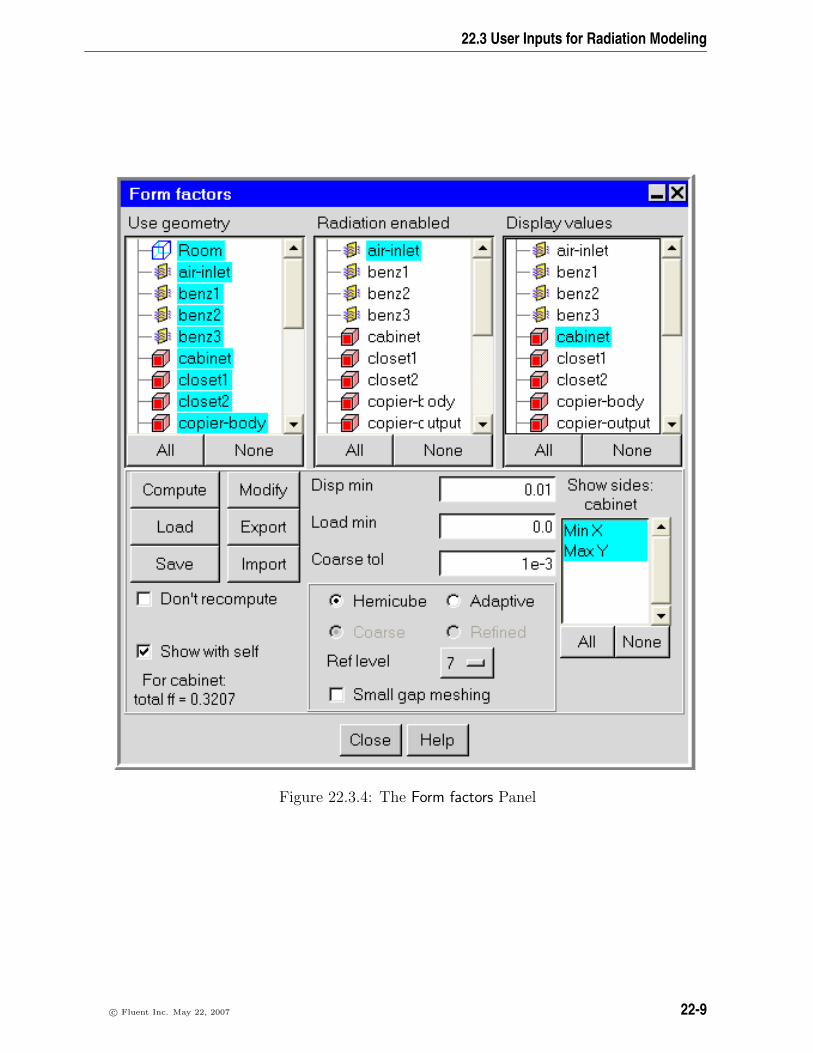
22.3 User Inputs for Radiation Modeling
Figure 22.3.4: The Form factors Panel
c© Fluent Inc. May 22, 2007 22-9

Radiation Modeling
Specifying the Objects to Include in the Radiation Calculation
All objects can receive radiant energy regardless of their ability to radiate energy them-selves. To specify that an object will receive radiant energy from other objects in themodel, click on the name of the object in the Use geometry list using the left mouse but-ton. Any object that has been specified to take part in the view factor calculation (i.e.,receive radiant energy) will be highlighted in blue in the Use geometry list. To includeall objects in the Use geometry list in the radiation calculation, click All at the bottom ofthe list. To deselect an object in the Use geometry list, click on the name of the objectin the Use geometry list using the left mouse button. To deselect all objects in the Usegeometry list, click None at the bottom of the list.
i If any sides of the room have been specified as wall, opening, or vent objects, youwill be able to include radiation to these sides. For those sides of the room thathave the Default specification (i.e., an adiabatic wall), radiant energy from otherobjects will be lost to these sides using a partial enclosure model. View factorcalculations will be disabled for these walls, which will instead be treated like ablack body with the default Radiation temperature specified in the Basic parameterspanel.
All the objects that can radiate energy are listed under Radiation enabled. To specifythat an object will radiate, click on the name of the object in the Radiation enabled listusing the left mouse button. Any object that has been specified to radiate to at leastone other object or surface will be highlighted in blue in the Radiation enabled list. Toinclude all objects in the Radiation enabled list in the radiation calculation, click All atthe bottom of the list. To deselect an object in the Radiation enabled list, click on thename of the object in the Radiation enabled list using the left mouse button. To deselectall objects in the Radiation enabled list, click None at the bottom of the list.
Computing View Factors
When you have selected the objects you want to participate in the radiation model, clickCompute to compute the view factors. The computation of the view factors may take afew seconds to a few minutes, depending on the size of the model.
To calculate the view factors, Airpak first creates a coarse mesh. It then discards thevolume mesh and coarsens the surface mesh. The Coarse tol option allows you to specifythe angular tolerance to be used during coarsening; i.e., it specifies the minimum anglebetween adjacent facets of the surface mesh for which coarsening will not happen. Asmall value allows higher accuracy, but Airpak will take more time to compute the mesh.A value of 1 (degree) is usually sufficient. To disable coarsening completely, enter a valueof −1.
22-10 c© Fluent Inc. May 22, 2007

22.3 User Inputs for Radiation Modeling
There are two methods available in Airpak for calculating the view factors: the hemicubemethod and the adaptive method. The hemicube method uses a differential area-to-areamethod and calculates the view factors on a row-by-row basis. The view factors calculatedfrom the differential areas are summed to provide the view factor for the whole surface.This method originated from the use of the radiosity approach in the field of computergraphics [8].
To use the hemicube method to compute the view factors, select Hemicube in the Formfactors panel. You can choose the refinement level to be used to calculate the view factors.To change the refinement level, click on the number to the right of Ref level in the Formfactors panel (Figure 22.3.4) and select a new number from the drop-down list. Thereare seven refinement levels available in Airpak. A higher level allows higher accuracy,but Airpak will take more time to compute the mesh. It is recommended that you usethe hemicube method for large complex models, because it is faster than the adaptivemethod for these types of models.
The adaptive method calculates the view factors on a pair-by-pair basis using a variety ofalgorithms (analytic or Gauss quadrature) that are chosen adaptively depending on theproximity of the surfaces. To maintain accuracy, the order of the quadrature increasesthe closer the faces are together. For surfaces that are very close to each other, theanalytic method is used. Airpak determines the method to use by performing a visibilitycalculation. The Gaussian quadrature method is used if none of the rays from a surfaceare blocked by the other surface. If some of the rays are blocked by the other surface,then either a Monte Carlo integration method or a quasi-Monte Carlo integration methodis used.
Two options are available in the Form factors panel for the Adaptive method: Coarse andRefined. If you select the Coarse option, 16 visibility samples will be taken from eachsurface. If you select the Refined option, 64 visibility samples will be taken from eachsurface. The calculation of the view factors will be significantly faster if you select theCoarse option, but the Refined option provides higher accuracy. It is recommended thatyou use the adaptive method for simple models, because it is faster than the hemicubemethod for these types of models.
If you make a change to your model and you do not want to recompute the view factorswhen you calculate a solution, select Don’t recompute in the Form factors panel.
Displaying View Factors
To view the computed view factors for an object, click on the name of the object in theDisplay values list. The name of the selected object will be displayed under Show sides,and the sides of the object that will participate in the radiation calculation will be listedin the Show sides list. Airpak displays arrows in the graphics window indicating whichobjects the selected object will radiate to, the names of the sides that are radiated to, andthe values of the view factors. An example is shown in Figure 22.3.5, where a partition
c© Fluent Inc. May 22, 2007 22-11

Radiation Modeling
will radiate to two blocks.
Figure 22.3.5: A Partition Radiates to Two Blocks
To display the view factors for all objects in the Display values list, click All at the bottomof the Display values list. To remove all the view factors from the graphics window, clickNone at the bottom of the Display values list. It is recommended that you select just oneor two objects at a time in the Display values list; otherwise, the display of view factorsin the graphics window will become cluttered. You can also display the view factors forjust one side of an object by first selecting the object in the Display values list and thenselecting the side of the object in the Show sides list. To display the view factors for allthe sides in the Show sides list, click All at the bottom of the Show sides list. To removethese view factors from the graphics window, click None at the bottom of the Show sideslist. If you select a heat sink object in the Display values list, Airpak will display the viewfactors for the radiation between the heat sink object and the other objects in the model,and also the view factors for the radiation between the parts of the heat sink object. Toremove the view factors for the radiation between the parts of the heat sink object fromthe graphics window, deselect Show with self in the Form factors panel (Figure 22.3.4).To redisplay these view factors, select Show with self.
Another way to control the number of view factors displayed in the graphics window is tospecify a value for Disp min or Load min. View factors that are smaller than the specifiedLoad min value will not be loaded into the Airpak model, and so cannot be viewed orused in the calculation. View factors that are smaller than the specified Disp min valuewill not be displayed in the graphics window, but they will be loaded into the model andused in the computation.
22-12 c© Fluent Inc. May 22, 2007

22.3 User Inputs for Radiation Modeling
Saving the Computed View Factors
To save the computed view factors, click Save. Airpak will save the view factors to afile. To reload the view factors, click the Load button. If you click Compute, Airpak willautomatically load the view factors after they have been computed.
To export the view factors to an ASCII file, click the Export button. You can reuse theASCII file in other Airpak jobs, and you can edit the file and add view factors to it usinga text editor. To import an ASCII file, click the Import button and select the file to beimported.
Modifying the Computed View Factors
If you want to modify the view factors, click Modify. This will open the Modify formfactors panel (Figure 22.3.6).
Figure 22.3.6: The Modify form factors Panel
You can modify any of the computed view factors by selecting the name of the surfacewhich is radiating in the From object list and the name of the surface which is beingradiated to in the To object list. Define the new view factor by entering a value in theValue text entry box and then click Modify. Modified view factors are shown in pink in
c© Fluent Inc. May 22, 2007 22-13

Radiation Modeling
the graphics window; the computed view factors are shown in blue. Click Reset to resetthe modified value back to the computed value.
22.4 Using the Discrete Ordinates Radiation Model
To solve a problem involving the discrete ordinates radiation model in Airpak, you willfollow the procedure outlined below:
1. Enable the calculation of radiation in the General setup tab of the Basic parameterspanel. To open the Basic parameters panel (Figure 22.3.1), double-click the Basicparameters item under the Problem setup node in the Model manager window.
Problem setup−→ Basic parameters
Enable the calculation of radiation by first turning On Radiation and then selectingDiscrete ordinates radiation model.
2. Specify the surface material to be used for each object in your model. This materialdefines the roughness and emissivity of the surface of the object.
By default, the material is specified as default for blocks, 2D sources, partitions,and walls. This means that the material specified on the surface of the object isdefined under Default surface in the Default values tab of the Basic parameters panel(see Section 6.4.7). To change the surface material for an object, select a materialfrom the material drop-down list. See Section 7.7 for details on material properties.
3. Define the rest of your problem in the usual way.
4. Start the calculation using the Solve panel. To open this panel, click on Startsolution in the Solve menu. Click Accept to start the calculation.
If you have enabled radiation in your model, you can turn off the calculation ofradiation by selecting the Disable radiation calculations option in the Solve panel.
Airpak will solve the transport equations for the discrete ordinates model once every fiveiterations in order to reduce the impact on the available computational resources. Airpakwill display the convergence history for the discrete ordinates equations (do-intensity) inthe Monitor graphics display and control window (see Section 27.12.2).
22.5 Modeling Solar Radiation Effects
Airpak’s solar load model allows you to include the effects of direct solar illumination aswell as diffuse solar radiation. Given the model geometry and pertinent solar informationsuch as terrestrial location, date, and time, the model performs a ray tracing shadingtest for all boundary surfaces. This approach includes a two-band (visible and infrared)spectral model for solar illumination. The transparent material model computes theabsorptivity and transmissivity as functions of incident angle.
22-14 c© Fluent Inc. May 22, 2007

22.5 Modeling Solar Radiation Effects
22.5.1 User Inputs for the Solar Load Model
To use the solar load model, follow the procedure outlined below.
1. Enable the calculation of radiation in the General setup tab of the Basic parameterspanel. To open the Basic parameters panel (Figure 22.3.1), double-click the Basicparameters item under the Problem setup node in the Model manager window.
Problem setup−→ Basic parameters
In the Basic parameters panel, turn on the Solar loading option and click Edit toopen the Solar Load Model parameters panel (Figure 22.5.1).
Figure 22.5.1: The Solar Load Model parameters Panel
2. In the Solar Load Model parameters panel, specify the following parameters underLocal time and position:
(a) Specify a value for the Date and select the month from the Month menu.
(b) Specify the local time at the desired location in the two fields to the rightof Time. The time is based on a 24-hour clock, thus acceptable values rangefrom 0 h 0 min (12:00 a.m.) to 23 h 59.99 min (11:59.99 p.m.). Values enteredin the first text-entry field (hour) must be integral, but values entered in thesecond text-entry field (minute) can be integral or fractional. For example, ifthe local time was 12:01:30 a.m., you would enter 0 for the hour and 1.5 forthe minute. If the local time was 4:17 p.m., you would enter 16 for the hourand 17 for the minute.
(c) (optional) Specify the local time zone of the desired location using the offsetvalue to the right of the Time entry fields. The options are: Greenwich Mean
c© Fluent Inc. May 22, 2007 22-15

Radiation Modeling
Time (GMT), Atlantic Standard Time (AST), Eastern Standard Time (EST),Central Standard Time (CST), Mountain Standard Time (MST), and PacificStandard Time (PST). The time zone is used to approximate the longitude(see below) of the location if you are unsure of the coordinates.
(d) Specify the Local Latitude of the desired location. Values can range from −90
(the South Pole) to 90 (the North Pole), with 0 defined as the equator. Selectthe hemisphere (N or S) from the menu to the right of the Local Longitude entryfield.
(e) Specify the Local Longitude of the desired location. The longitude is approx-imated if you specify the local time zone, but you can enter a more precisevalue if you know it. Any value you enter here will take precedence over thetime zone. Values may range from 0 to 180. Select the hemisphere (W or E)from the menu to the right of the Local Longitude entry field.
3. Under Illumination parameters, specify the following parameters:
(a) Specify the Sunshine fraction, which is a factor between 0 and 1 used to accountfor the effects of clouds which may reduce the direct solar irradiation. Clearsky is modeled by setting the value equal to 1 and complete cloud cover ismodeled by setting the value equal to 0. Partial cloud cover is modeled bysetting the value to be between 0 and 1. The default value is 1.0.
(b) Specify the Ground reflectance, which is a parameter that is used in determininghe contributions of reflected solar radiation from ground surfaces. Reflectedsolar radiation from ground surfaces is a function of the direct normal irra-diation, the time of the year, the tilt angle of the surface, and the groundreflectance. It is treated as part of the total diffuse solar irradiation. Groundreflectance values can vary depending on the ground surface (i.e., concrete,grass, rock, gravel, asphalt). The default value is 0.2.
4. Specify the solar classification of all room objects in each Object panel. For eachobject, select one of the following options next to Solar behavior:
Insulator indicates that the surface will not be considered in the solar radiationmodeling.
Opaque indicates that the surface will not allow solar radiation to pass throughit.
Transparent indicates that the surface will allow a portion of the solar radiationto pass through it.
5. Specify the surface material to be used for each object or surface. This surfacematerial defines the roughness, emissivity, and the absorption and transmission pa-rameters of the surface. If the material is opaque, you will specify the absorptivitiesin the visible and infrared portions of the spectrum. If the material is transparent,you will specify the visible transmittance and shading coefficient.
22-16 c© Fluent Inc. May 22, 2007

22.5 Modeling Solar Radiation Effects
By default, the material is specified as default for blocks, 2D sources, partitions,and walls. This means that the material specified on the object or surface is definedunder Default surface in the Default values tab of the Basic parameters panel (seeSection 6.4.7). To change the material for an object or surface, select a materialfrom the material drop-down list. See Section 7.7 for details on material properties.
6. Define the rest of the problem in the usual way.
c© Fluent Inc. May 22, 2007 22-17

Radiation Modeling
22-18 c© Fluent Inc. May 22, 2007

Chapter 23. Optimization
Airpak uses the Dynamic-Q optimization method to solve constrained-design-optimizationproblems. See Section 31.5 for details about the theory behind Airpak’s optimizationmethod.
Information about solving design-optimization problems using Airpak is presented in thefollowing sections:
• Section 23.1: When to Use Optimization
• Section 23.2: User Inputs for Optimization
23.1 When to Use Optimization
Design optimization can be used for a variety of CFD problems. Some examples includethe following:
• Placement of airflow supplies
• Placement of airflow returns
• Optimizing supply temperatures
• Optimizing system airflow rates
• Optimizing floor tile percentage open in data centers
• Optimizing exhaust airflow rates
Airpak’s optimization method is particularly suited for problems with a large numberof design variables and constraint functions. The maximum number of design variablesallowed is 50 and the maximum number of constraint functions is 10.
c© Fluent Inc. May 22, 2007 23-1

Optimization
23.2 User Inputs for Optimization
To solve an optimization problem in Airpak, you will follow the procedure outlined below.
1. Define all the required design variables in the appropriate input fields in the sameway you would define parameters. For more information on how to define parame-ters see Section 24.2.
i Note that boolean parameters and fan failure cannot be defined as designvariables for optimization problems.
2. To enable the optimization, select Optimization in the Setup tab of the Parame-ters and optimization panel. To open the Parameters and optimization panel (Fig-
ure 23.2.1), select Run optimization in the Solve menu or click the button inthe Model and solve toolbar.
Solve−→Run optimization
3. Define the range of design variables.
(a) Select the design variable from the list in the Design variables tab of the Pa-rameters and optimization panel (Figure 23.2.2). Expanding a design variable’stree node displays objects and properties associated with the variable.
(b) Specify the starting value of the variable in the Base value text box.
(c) Specify the minimum and maximum values the variable can take in the Minvalue constraint and Max value constraint text boxes.
(d) If the design variable can only take values in multiples of a number, selectAllow only multiples and specify the lowest multiple in the provided text box.For example, the fin count for a heatsink can be specified only in multiplesof 1.
23-2 c© Fluent Inc. May 22, 2007

23.2 User Inputs for Optimization
Figure 23.2.1: The Parameters and optimization Panel (Setup Tab)
c© Fluent Inc. May 22, 2007 23-3

Optimization
Figure 23.2.2: The Parameters and optimization Panel (Design variables Tab)
23-4 c© Fluent Inc. May 22, 2007

23.2 User Inputs for Optimization
4. Define functions in the Functions tab of the Parameters and optimization panel (Fig-ure 23.2.3). These functions will be set as objective or constraint functions.
Figure 23.2.3: The Parameters and optimization Panel (Functions Tab)
Functions are classified as Primary functions and Compound functions. Primary func-tions can be defined using design variables and accessible solution data. Compoundfunctions are functions of Primary functions. Compound functions cannot be createdwithout creating Primary functions.
c© Fluent Inc. May 22, 2007 23-5

Optimization
(a) To create a primary function, click the New button under Primary functions.This will open the Define primary function panel (Figure 23.2.4).
Figure 23.2.4: The Define primary function Panel
i. Primary functions can be defined in different ways by selecting one of thefollowing options in the Define primary function panel:
Pre-defined function allows you to define a primary function by select-ing one of the following Airpak pre-defined functions from the drop-down list: Global maximum temperature, Maximum temperature of ob-jects, and Mean temperature of objects (see Figure 23.2.5).
Figure 23.2.5: The Pre-defined function drop-down list
23-6 c© Fluent Inc. May 22, 2007

23.2 User Inputs for Optimization
Pre-defined report allows you to define a primary function by selectingone of the user pre-defined summary reports from the drop-down list,and by selecting one of the following functions corresponding to thereport: Min, Max, Mean, St dev, and Total. See Section 27.10 for moreinformation on defining summary reports.
Pre-defined post objects allows you to define a primary function by se-lecting one of the user pre-defined post objects from the drop-downlist (e.g., object faces and plane cuts), and by selecting one of thefollowing functions corresponding to the object: Min, Max, Mean, Stdev, and Total. See Section 27.9 for more information on defining postobjects.
Point report allows you to define a primary function by selecting oneof the user defined point reports from the drop-down list. See Sec-tion 28.2.7 for more information on defining point reports.
Design variable allows you to define a primary function by selecting oneof the design variables from the drop-down list. See Section 24.5 formore information on defining design variables.
Object property allows you to define a primary function by selecting anobject from the Object drop-down list, and by selecting an appropriateobject property from the Property drop-down list. Only certain objectproperties (e.g., geometry, power, and radiation parameters) can beused to define primary functions.
Difference function allows you to define a primary function using differ-ences of mean values of post-processing variables across two opposingfaces of an object. To use the difference function, select an Object,Variable, and Direction from the drop-down lists. The function valueis calculated by subtracting the mean values of a post-processing vari-able computed across two sides of an object (e.g., High X and LowX). For example, this function can be used to determine the pressuredrop across a heatsink by selecting the difference in the pressures atthe leading and trailing sides of the heatsink.
ii. If this is a constraint function, check the Constraint box, click Min valueor Max value, and enter the constraint value.
(b) To create a compound function, click the New button under Compound func-tions. This will open the Define compound function panel (Figure 23.2.6). In theDefine compound function panel. Specify the Function name and the Definitionof the compound function. To define the compound function, the appropriateprimary functions should be used. In the Definition box, the primary functionname must be proceded by a $ sign.
(c) Specify an objective function.
c© Fluent Inc. May 22, 2007 23-7

Optimization
Figure 23.2.6: The Define compound function Panel
i. Select one of the previously defined functions from the Objective functiondrop-down list, in the Parameters and optimization panel (Figure 23.2.3).
ii. To maximize the objective function, select Maximize value, otherwise, theobjective function will be minimized by default.
i Note that if a function is neither a constraint function nor an objective func-tion, the function value is merely reported with the optimization results.
5. Choose which functions to make inactive or active.
(a) To make a function inactive, choose the function under Selected functions inthe Parameters and optimization panel (Figure 23.2.3) and place the function inthe Inactive functions list by clicking the Remove button. Note that placing thefunction in the Inactive functions list does not delete the function. Functionsplaced in the Inactive functions list are not reported with the optimizationresults.
(b) To activate a function, choose the function under Inactive functions and clickthe Add button.
i To delete a function, select the function under Primary functions or Compoundfunctions and click the Delete button.
6. Start the optimization process by clicking the Run button in the Parameters andoptimization panel.
When Airpak starts performing calculations, the Optimization run window will openand Airpak will display all the function values, design variables, and the runningtimes for each optimization iteration. In addition, the function values and designvariables are plotted versus iteration number. The plots are displayed on the lefthand side of the Optimization run window (Figure 23.2.7).
The graphics window is fully interactive. For example, at any time during thecalculation, you can zoom in on a specific portion of the graph. This graphicswindow is similar to the Monitor graphics display (see Section 27.12.2).
Other options available in this window include
23-8 c© Fluent Inc. May 22, 2007

23.2 User Inputs for Optimization
Figure 23.2.7: The Optimization run Panel
• turning off variation of certain function or variable values as a function ofoptimization iteration number, and
• plotting of design variables.
To turn off the display of certain variation plots of functions or variables as functionsof iteration number (e.g., objective function, design variables), click the legend lineshowing the function or variable. To display the variable again, click the appropriatelegend line.
To plot a design variable against a function, click the Plot button in the Optimizationrun window. From Selection panels, select the x axis and y axis variables. Theplots show the variation of the design variables against the selected function foreach constant value of the remaining variables. For more information on plottingand reporting of design variables see Section 24.9.
c© Fluent Inc. May 22, 2007 23-9

Optimization
23-10 c© Fluent Inc. May 22, 2007

Chapter 24. Parameterizing the Model
Airpak allows you to parameterize your model, so that you can determine the effect ofvarious object sizes or other characteristics on the solution.
Information about parameterization is divided into the following sections:
• Section 24.1: Overview of Parameterization
• Section 24.2: Defining a Parameter in an Input Field
• Section 24.3: Defining Check Box Parameters
• Section 24.4: Defining Radio Button Parameters (Option Parameters)
• Section 24.5: Defining a Parameter (Design Variable) Using the Parameters andoptimization Panel
• Section 24.6: Deleting Parameters
• Section 24.7: Defining Trials
• Section 24.8: Running Trials
• Section 24.9: Function Reporting and Plotting
24.1 Overview of Parameterization
A design process requires the evaluation of a number of available options to determinethe most appropriate case that meets the primary design requirement (e.g., smallest sizeof the room, lowest fan speed that cools the given system to the specified temperature,smallest vent size that meets the system requirements). All of these design scenariosrequire you to change different parameters and calculate multiple solutions to optimizethe design. By studying the results of these multiple calculations, you can identify thetrends that affect the performance of the system and you can optimize the design of yourmodel.
Airpak provides a convenient way to specify the range of values for geometric sizes andlocations, boundary conditions (e.g., fan curves, vent loss coefficients), and materialproperties in a single model building exercise. Airpak then instructs the solver to run thedifferent trials that you selected. This process saves the time required to build or specifyeach model separately and run each of the trials yourself in a sequential manner.
c© Fluent Inc. May 22, 2007 24-1

Parameterizing the Model
Parameters in Airpak are numeric or string constants that you can use in your modelinstead of actual numeric or string inputs, so that you can easily change their values tomodel different designs. For example, if you wanted to assign the flow rate for a fan to bethe numeric value 0.01, you can specify a parameter called flowrate and assign a value of0.01 to this parameter. You can assign more than one value to a parameter, to define trialcalculations that you want to perform for your model. Each trial represents a combinationof parameter values, so it is possible to perform multiple trials for your model. In addition,different design scenarios can be tested parametrically by parameterizing check-box andradio-button options. For example, the effect of changing the type of a diffuser assemblyin a design, from a round ceiling diffuser to a linear slot diffuser, can be tested byperforming two trials, made by turning on/off appropriate diffusers. Similarly, the effectof turbulence can be tested by setting up a parameter for Flow regime radio buttons inthe Basic parameters panel.
There are four ways to define a parameter in Airpak:
• Enter a parameter in an input field for an object, material, problem setup default,or solver default (Section 24.2).
• Enter a check box parameter for an object, material, or problem setup default(Section 24.3).
• Enter a radio button parameter (Option Parameter) for a problem setup default(Section 24.4) or solver default.
• Define a parameter in the Parameters and optimization panel (Section 24.5).
i Note that parameters can be used for all inputs for all objects, but they cannot beused for macros.
Once the parameters have been defined, you can redefine the initial value and specifyadditional values using the Parameters and optimization panel (Section 24.5).
You can use the parameters to define the trial calculations that you want to performfor your model (Section 24.7), and finally, you can instruct Airpak to run the trials(Section 24.8) and to plot the results (Section 24.9).
24.2 Defining a Parameter in an Input Field
A parameter can be defined in an input field for any object, material, problem setupdefaults, and solver defaults. For example, if you want to specify a parameter for thevolume flow rate of a fan, you can define a parameter called flowrate in the Volume textentry field next to the Fixed, under Flow rate, in the Fans panel, as shown below.
24-2 c© Fluent Inc. May 22, 2007

24.2 Defining a Parameter in an Input Field
You can specify any combination of alphanumeric characters and symbols (except spaces)for the parameter name.
i When you specify a parameter in the input field for an object or material, you mustalways preface the parameter name with the $ sign. For instance, in the exampleabove, the input for the volume flow rate for the fan is $flowrate. If you specifya parameter for a scaling factor when defining the anisotropic conductivity of amaterial, you must enclose the scaling factor parameter in in the Tensor field inthe Materials panel. An example is shown below.
c© Fluent Inc. May 22, 2007 24-3

Parameterizing the Model
If the parameter you define is related to the geometry of an object or the properties of amaterial, Airpak will ask you to enter a value for the parameter when you click Update orDone in the Object panel or the Materials panel. For example, if you specify a parameterfor the radius of the fan ($radius), Airpak will ask you to provide an initial value for theradius in the Param value panel (Figure 24.2.1).
Figure 24.2.1: The Param value Panel
When you click Done in the Param value panel, Airpak will update the display of theobject in the graphics window using the specified initial value. You can define more thanone value for a parameter using the Parameters and optimization panel (see Section 24.5).
If the parameter you specified is related to the physical characteristics of the object(excluding the geometry), Airpak will set the initial value of the parameter to be zero.You will then be prompted to enter an initial value for the parameter upon openingthe Parameters and optimization panel. You can redefine the initial value and specifyadditional values using the Parameters and optimization panel (see Section 24.5).
Simple arithmetic operations such as addition, division, and multiplication can be usedwith a combination of parameters and/or numeric inputs. For example, you can specifythe volume flow rate for the fan to be equal to
($a*($flowrate)/ $b + 0.1)
i If you use an arithmetic expression to define a parameter, the expression must beenclosed in parentheses.
24-4 c© Fluent Inc. May 22, 2007

24.3 Defining Check Box Parameters
i Note that, by default, integer arithmetic is performed for division if both thedivisor and dividend are entered as integers. If you want floating point division tobe performed, then either the divisor or dividend should be entered as a floatingpoint number. For example, $a/10 will give a quotient of 0 if $a is defined as 1,while $a/10.0 will give a quotient of 0.1 if $a is 1.
Note that the definition of a parameter is independent of units; i.e., parameters arepurely numeric inputs. In the above example for the volume flow rate of a fan, Airpakwill calculate the expression
($a*($flowrate)/ $b + 0.1)
by substituting the values of the parameters into the expression and then the unit (e.g.,ft3/s) will be added to the final value of the expression.
To allow you to most efficiently define common parameters for copies of an object, Airpakwill automatically copy the parameters that you have defined for an object when youcopy the object. The copied parameters will then be used for all copies of the object,rather than using the current parameter values. Parameters used for geometric entrieswill automatically be summed to the values of the corresponding geometric entries thatyou will request for each copy of the object. For example, if you define the geometric xEcoordinate of an object with a parameter $a and then make copies of the object that aretranslated in the x direction, then the xE field for the copies will be
$a + d
where d is the prescribed offset of the copy of the object.
24.3 Defining Check Box Parameters
A parameter can be defined to turn on/off a check box parametrically. To define acheck box parameter, right-click any check-box option in the Object, Materials, or Basicparameters panel. For example, to define the existence or non-existence of an object,position the cursor directly over the Active checkbox in the Info tab of the Object paneland right-click the Active check box to open the Active parameter panel (Figure 24.3.1).
There are two ways to define the Active parameter:
• Specify the variable name that will be set to be equal to the object’s name. In theActive parameter panel, select Option is ON if variable is equal to this object’s name,and enter the Variable name. Airpak will ask you to provide an initial value for thevariable in the Param value panel (Figure 24.2.1). The name of the object or someother name must be entered, enclosed within quotation marks.
• Specify an expression and the numeric value of the expression. In the Active param-eter panel, select Option is ON if expression is equal to a specified value, and enter
c© Fluent Inc. May 22, 2007 24-5

Parameterizing the Model
Figure 24.3.1: The Active parameter Panel
the Expression and the Value. Also, provide an initial value for the variable in theParam value panel (Figure 24.2.1).
i Note that the variable name and the expression must be preceded by a $ sign.
To turn off the parameterization for a check box, first select Not Parametrized, then selectOn.
Examples1. Consider a model with two air supply diffuser assemblies (round ceiling and linear
slot). To selectively turn on/off the activity of the diffusers, you can define theactive parameters as follows:
(a) Set the parameter values for the round ceiling diffuser to 0 (not active) and1 (active). Open the Active parameter panel for the diffuser.1, and selectOption is ON if expression is equal to a specified value. In the Expression entrybox enter $round on, and in the Value entry box enter 1, as shown in Fig-ure 24.3.2. Airpak will ask you to provide an initial value for the variable inthe Param value panel. Enter 1 and click Done. To set another value of theparameter to 0, for which the diffuser assembly will not be Active, you will useParameters and optimization panel (see Section 24.5).
(b) Set the parameter values for the linear slot diffuser assembly to "diffuser.2"
(active) or "off" (not active). As described above, open the Active parameterpanel for the diffuser.2, and select Option is ON if variable is equal to this
24-6 c© Fluent Inc. May 22, 2007

24.3 Defining Check Box Parameters
Figure 24.3.2: The Active parameter Panel for the Round Ceiling Diffuser
object’s name. In the Variable name entry box enter $linear on, as shown inFigure 24.3.3. Airpak will ask you to provide an initial value for the variablein the Param value panel. Enter "diffuser.2" and click Done. To set anothervalue of the parameter to "off", for which the diffuser assembly will not beActive, you will use Parameters and optimization panel (see Section 24.5).
Figure 24.3.3: The Active parameter Panel for the Linear Slot Diffuser
2. This example will demonstrate the use of boolean expressions. Consider a modelwith five partitions in which you would like to replace one partition with a resistancein each of five trials by selectively turning on/off the activity of partitions and
c© Fluent Inc. May 22, 2007 24-7

Parameterizing the Model
resistances. Five resistances need to be defined with the same locations as thepartitions. You can define the active parameters as follows:
(a) For each partition, respectively, define the folowing boolean expressions in theActive parameter panel, under Expression, after selecting Option is ON if ex-pression is equal to a specified value: ($resistance!=1), ($resistance!=2),($resistance!=3), ($resistance!=4), and ($resistance!=5). Under Value,enter 1 for every partition, which means logical true (every other number isfalse). After you specified the expression for the first partition, Airpak willask you to provide an initial value for the variable in the Param value panel.Enter 1 and click Done.
(b) For each resistance, respectively, define the folowing boolean expressions inthe Active parameter panel, under Expression, after selecting Option is ON if ex-pression is equal to a specified value: ($resistance==1), ($resistance==2),($resistance==3), ($resistance==4), and ($resistance==5). Under Value,enter 1 for every resistance. To set values of the parameter to 2, 3, 4, and 5
to determine which vent will be active in each trial, you will use Parametersand optimization panel (see Section 24.5).
i Note that a check box parameter in the Basic parameters panel can only be definedusing an expression and a numeric value of the expression.
24.4 Defining Radio Button Parameters (Option Parameters)
A parameter can be defined to select a radio-button option, parametrically, from theBasic parameters, Parallel settings, or Advanced solver setup panel. To define an Optionparameter, right-click any radio-button option in the Basic parameters, Parallel settings, orAdvanced solver setup panel. For example, to define the Flow regime parametrically, right-click the Laminar or Turbulent radio button, next to Flow regime, in the Basic parameterspanel. This will open the Option parameter panel (Figure 24.4.1).
In this panel, specify the expression that represents the name of the parameter(e.g.,flow regime). The value of the expression will determine the option. The defaultvalue of the parameter is 0. The options, along with the values that enable them, arelisted in the panel (Figure 24.4.1). For example, the default value of the flow regimeparameter is 0, which enables Laminar flow. To set another value of the parameter to 1,which enables Turbulent flow option, you will use Parameters and optimization panel (seeSection 24.5).
i Note that the expression must be preceded by a $ sign.
i If the value of the specified expression is not equal to any of the predefined valueslisted in the Option parameter panel, then the default option is used for that value.
24-8 c© Fluent Inc. May 22, 2007

24.5 Defining a Parameter (Design Variable) Using the Parameters and optimization Panel
Figure 24.4.1: The Option parameter Panel
24.5 Defining a Parameter (Design Variable) Using the Parameters andoptimization Panel
You can define additional new parameters, also called design variables, or edit existingparameters using the Parameters and optimization panel (Figures 24.5.1, 24.5.2). To open
this panel, click the button in the Model and solve toolbar.
In the Design variables tab, the Parameters and optimization panel displays all the param-eter names that are currently defined, along with their associated values (Figure 24.5.2).
To define a new parameter, click the New button in the Design variables tab, and enterthe name of the parameter in the New variable name? text entry field in the Query dialogbox. Airpak will add the new parameter to the list in the Parameters and optimizationpanel. You can specify any combination of alphanumeric characters and symbols (exceptspaces) for the parameter name. Enter the value(s) of the parameter. There are twoways of specifying values for parameters:
• Select Discrete, and in the text entry field enter multiple values for a parameterseparated by commas or spaces.
• Select In range, and enter Start value, End value, and Increment.
Click Apply to update the list of available trials corresponding to the new set of parameters(see Section 24.7).
To edit previously defined parameters, enter the new value for the parameter in thecorresponding Base value field. You can then enter multiple values for a parameter usingone of the above two methods.
Opening up a design variable’s tree displays the object(s) and properties associated withthe variable.
c© Fluent Inc. May 22, 2007 24-9

Parameterizing the Model
Figure 24.5.1: The Parameters and optimization Panel (Setup Tab)
i Note that you can use a parameter in the definition of another parameter’s values,but you must precede the parameter name with a $ sign in the Base value field ofthe Parameters and optimization panel.
24.6 Deleting Parameters
If you have parameters defined in your model that you no longer need, you can deletethese parameters from your model. To delete a parameter, select the parameter in theDesign variables tab of the Parameters and optimization panel (Figure 24.5.2), and clickthe Delete button.
Airpak will delete the parameter only if it is not being used anywhere in your model.
24-10 c© Fluent Inc. May 22, 2007

24.7 Defining Trials
Figure 24.5.2: The Parameters and optimization Panel (Design variables Tab)
To delete all parameters (design variables) and replace all their uses with their presentvalues, click the Delete all variables button.
24.7 Defining Trials
Parameters in Airpak are used to define the trial calculations that you want to perform foryour model. Each trial represents a combination of parameter values. Airpak calculatespossible combinations from the list of parameters specified in the Design variables tabof the Parameters and optimization panel and lists them in the Trials tab of the panel(Figure 24.7.1). Alternatively, you can select Define trials in the Solve menu.
Solve−→Define trials
c© Fluent Inc. May 22, 2007 24-11

Parameterizing the Model
Figure 24.7.1: The Parameters and optimization Panel (Trials Tab)
There are two ways of listing possible combinations from the list of parameters specified inthe Design variables tab of the Parameters and optimization panel: listing all combinationsand listing ”by column”. To choose one of the two options, select Parametric trials in theSetup tab of the Parameters and optimization panel (Figure 24.5.1).
All combinations lists all possible combinations from the list of parameters specified inthe Design variables tab of the Parameters and optimization panel.
By Column controls the number of trial combinations, by selecting Variable is ”bycolumns” for certain parameters in the Design variables tab. If this option is se-lected for some of the parameters, then the number of trial combinations will bethe number of all possible combinations of parameters that are not defined ”bycolumn” (i.e., parameters for which the option Variable is ”by columns” is not se-lected). For example, if you define the parameters p, u, and v that can take thefollowing values:
24-12 c© Fluent Inc. May 22, 2007

24.8 Running Trials
p = 10, 20, 30 (24.7-1)
u = 1, 2, 3, 4
v = 100, 200
then
if p is defined ”by column”, there would be 4 ∗ 2 = 8 trials;if u is defined ”by column”, there would be 3 ∗ 2 = 6 trials;if v is defined ”by column”, there would be 3 ∗ 4 = 12 trials,if both p and u are defined ”by column”, there would be 2 trials;if both p and v are defined ”by column”, there would be 4 trials;if both u and v are defined ”by column”, there would be 3 trials.
If a parameter that had been defined ”by column” has fewer defined values thanthe combination of other parameters, Airpak will use the last value specified forthat parameter until all trials have been defined.
24.7.1 Selecting Trials
Select the trials that you want to run from the list of possible trials in the Trials tab ofthe Parameters and optimization panel (Figure 24.7.1). Turn the Select option on or offfor a trial in the list to toggle its selection state. Click on Set above a trial to make itthe first one to be run by Airpak. Note that as you click Set for a particular trial, Airpakwill update the graphics window to reflect the geometry that is defined by the valuesof the parameters used in that trial. This allows you to inspect the effect of changes tothe geometry of objects in the model corresponding to each trial. To further change theorder in which the trials are run, you can enter the appropriate values in the text boxesnext to Order.
To speed up convergence of subsequent trials, you can run any trial (except for the firstone) using the solution from a previous trial as an initial condition. To do so, select theTrial Name corresponding to the solution you want to use for restart from the Restart IDdrop-down list of the new trial (e.g., Figure 24.7.2).
24.8 Running Trials
Once you have selected the trials that you want to run, you will instruct Airpak to runthe trials.
c© Fluent Inc. May 22, 2007 24-13
Parameterizing the Model
Figure 24.7.2: The Parameters and optimization Panel Displaying Restart IDOptions (Trials Tab)
24-14 c© Fluent Inc. May 22, 2007

24.8 Running Trials
24.8.1 Running a Single Trial
To run a single trial in your Airpak model, follow the steps below.
1. Select Single trial (current values) in the Setup tab of the Parameters and optimizationpanel (Figure 24.5.1).
2. (optional) To request that Airpak generate one or more function values after therun, define the appropriate function in the Functions tab of the Parameters andoptimization panel, as described in Chapter 23.
3. Set the solver controls for the trial. You will use the Solve panel to set the solvercontrols. (See Section 27.11 for more details on setting the solver controls.) Toopen the Solve panel, select Run solution in the Solve menu.
Solve−→Run solution
(a) To view information about the trial that will be performed, click the Trial infobutton in the Solve panel. Airpak will list information about the trial in theMessage window and also open the Parameters and optimization panel if it isnot already displayed.
(b) If you want Airpak to generate a report when the trial is complete, select Writereport when finished in the Solve panel. See Section 27.10 for details on defininga report to be generated when the calculation is complete.
(c) Click Start solution in the Solve panel to start the calculation.
i You can also start the solution from the Parameters and optimization panel byclicking the Accept button. This will open the Start solution panel. To start thesolution click Yes.
Airpak will set the values of the parameters to those specified for the trial selected in theTrials tab of the Parameters and optimization panel (Figure 24.7.1), and then perform thecalculation. When the calculation is finished, Airpak will save the results of the simulationand generate a function report (if requested) and display it on the screen. It will alsogenerate a summary report (if requested). You can then perform postprocessing in theusual way (as described in Chapter 28) and you can view the results of the reports thatAirpak has generated, as described in Section 29.5.
You can also stop the solver during the trial calculation using the Terminate button in theMonitor window (see Section 27.12.2 for details). The message Solution (projectname)
is finished appears in the Message window when the solver is done. Note that theMonitor windows will remain open until you close them by clicking Done.
c© Fluent Inc. May 22, 2007 24-15

Parameterizing the Model
24.8.2 Running Multiple Trials
To run multiple trials for your Airpak model, follow the steps below.
1. Select Parametric trials in the Setup tab of the Parameters and optimization paneland select one of the two options: All combinations or By columns. For more detailson defining trials see Section 24.7.
2. Select the trials to be run in the Trials tab of the Parameters and optimization panel(Figure 24.7.1), as described in Section 24.7.1. At this point, you may want totoggle the naming scheme of the trials, by clicking on Reset. The Trial namingdialog will open, and you will be able to choose between Numbered (the defaultnaming scheme, see, for example Figure 24.7.2), or Value, a naming scheme thatuses values of the parameters in each trial name.
3. (optional) To request that Airpak generate one or more function values after therun, define the appropriate function in the Functions tab of the Parameters andoptimization panel, as described in Chapter 23.
4. Set the solver controls for the trials. You will use the Solve panel to set the solvercontrols. (See Section 27.11 for more details on setting the solver controls.) Toopen the Solve panel (Figure 24.8.1), select Run solution in the Solve menu.
Solve−→Run solution
(a) Select the Perform multiple trials option in the Solve panel. You can viewinformation about the trials that will be performed if you click the Trial infobutton in the Solve panel. Airpak will list trial information in the Messagewindow, including the number of trials to be performed, which variables areused, the values specified for each variable, and the values of the variables forthe trials to be performed.
(b) If you are running Airpak on a multiprocessor machine, you can specify thenumber of trials that Airpak should run simultaneously on your machine in theNum concurrent text entry field in the Solve panel. For example, if you enter2 in the Num concurrent field, Airpak will run two trials simultaneously. Whenone of the trials has finished, Airpak will start the third trial, and so on.
i Note that the number of trials that Airpak can run simultaneously islimited by the number of available Airpak licenses.
(c) If you have chosen to submit multiple trials to a script file, you may want toturn on the Launch from script option. If this option is enabled, Airpak willautomatically launch the script file after all of the case files have been writtenfor the different trials. This option will be useful in times when you lock thescreen after instructing Airpak to write a script file for running multiple trials.
24-16 c© Fluent Inc. May 22, 2007

24.8 Running Trials
Figure 24.8.1: The Solve Panel
(d) If the trials do not involve changes to the model geometry, enable the Use fasttrials if possible option in the Advanced tab of the Solve panel. This will reducethe time taken per trial and also reduce the memory storage space becauseonly a single case file will be written. If this option is disabled, a separatemesh will be created and a separate case file will be written for every trialregardless of whether the geometry has changed or not.
(e) If you want Airpak to generate a report when each trial is complete, select Writereport when finished in the Options tab of the Solve panel. See Section 27.10 fordetails on defining a report to be generated when the calculation is complete.
(f) Click Start solution in the Solve panel to start the calculation.
i You can also start the solution from the Parameters and optimization panel byclicking the Accept button. This will open the Start solution panel. To start thesolution click Yes.
c© Fluent Inc. May 22, 2007 24-17

Parameterizing the Model
If you entered 1 next to Num concurrent in the Solve panel, Airpak will set the valuesof the parameters to those specified for the first trial selected in the Trials tab of theParameters and optimization panel (Figure 24.7.1), and then start the calculation, using asolution ID of trial000. When the calculation is finished, Airpak will save the results ofthe simulation and generate a report or a function value (if requested). Airpak will thenset the values of the parameters to those specified for the second trial in the Trials tabof the Parameters and optimization panel, and start a new calculation. When this calcu-lation is complete, Airpak will save the results of the simulation using a new solution ID(trial001), and generate a report. This process of setting the values of the parameters,performing the calculation, saving the results, and generating reports is repeated untilall the selected trials have been completed.
If you have specified that Airpak should run two or more calculations simultaneously,Airpak will set the values of the parameters to those specified for the first trial selectedin the Trials tab of the Parameters and optimization panel (Figure 24.7.1), and then startthe calculation, using a solution ID of trial000, Airpak will then set the values ofthe parameters to those specified for the second trial selected in the Trials tab of theParameters and optimization panel, and start a second calculation with a new solutionID (trial001), and so on. When the first calculation is finished, Airpak will save theresults of the simulation and generate a report (if requested). Airpak will then set thevalues of the parameters to those specified for the next trial selected in the Trials tabof the Parameters and optimization panel, and start a new calculation. When the secondcalculation is complete, Airpak will save the results of the simulation, generate a report(if requested), and start the next trial, and so on. This process of setting the values ofthe parameters, performing the calculation, saving the results, and generating reports isrepeated until all the selected trials have been completed.
You can then perform postprocessing in the usual way, specifying which trial results youwant to examine by selecting the appropriate solution ID. See Section 28.4 for details.You can also view the results of the reports that Airpak has generated, as described inSection 29.5.
You can stop the solver during the trial calculations using the Terminate button in theMonitor window (see Section 27.12.2 for details). All trial runs are terminated, and themessage Solution (projectname) is finished appears in the Message window whenthe solver is done. Note that the Monitor windows will remain open until you close themby clicking Done.
24.9 Function Reporting and Plotting
As Airpak starts performing the trials, the Parametric trials panel will open and Airpakwill display all the function values defined a priori, as well as parameters and runningtimes for each trial (Figure 24.9.1).
The function values reported in the Parametric trials panel can be plotted against the
24-18 c© Fluent Inc. May 22, 2007

24.9 Function Reporting and Plotting
Figure 24.9.1: The Parametric trials Panel
c© Fluent Inc. May 22, 2007 24-19

Parameterizing the Model
parameters. To create plots of functions versus parameters, follow the steps below:
1. If the Parametric trials panel is not already opened, select Show optimization/paramresults from the Report menu to open the Parametric trials panel.
Report−→Show optimization/param results
2. In the Parametric trials panel (Figure 24.9.1), click the Plot button to open theSelection panel (Figure 24.9.2). In the Selection panel, select the design variable forthe x axis (e.g., Thickness), and click Okay.
Figure 24.9.2: The Select Panel (x axis selection)
3. In the Selection panel (Figure 24.9.3), select the function for the y axis (e.g., Kloss)and click Accept. This will display the plot (e.g., Kloss vs Thickness), as shown inFigure 24.9.4. For more information on modifying the range and appearance of theplot, printing, saving, and reloading plot data, see Section 28.3.2.
Figure 24.9.3: The Select Panel (y axis selection)
4. To display another plot, click the Plot button in the Parametric trials panel again,and repeat steps 2 and 3, to make x and y axis selections. You can repeat this stepmultiple times, which will allow you to view multiple plots at the same time.
24-20 c© Fluent Inc. May 22, 2007
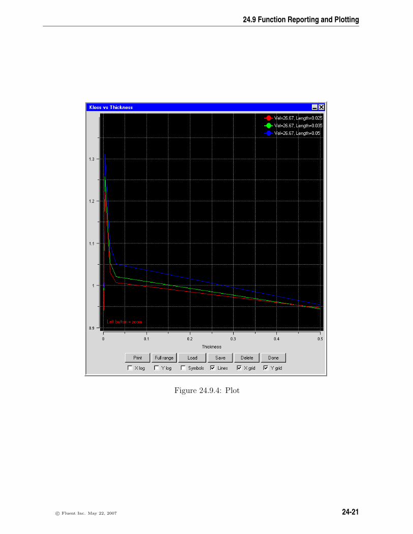
24.9 Function Reporting and Plotting
Figure 24.9.4: Plot
c© Fluent Inc. May 22, 2007 24-21

Parameterizing the Model
24-22 c© Fluent Inc. May 22, 2007

Chapter 25. Using Macros
Macros can help streamline the process of building your Airpak model. There are threegeneral types of macros you can choose from that are accessible from the Macros menu.
This chapter describes the macros available in Airpak and how you can use them. Infor-mation in this chapter is organized into the following sections:
• Section 25.1: Boundary Condition Macros
• Section 25.3: Geometry Macros
• Section 25.4: Object Rotation Macros
25.1 Boundary Condition Macros
The following boundary condition-related macros are described in the following sections:
• Section 25.1.1: Solar Flux Boundary Condition
• Section 25.1.2: Atmospheric Boundary Layers
• Section 25.2: Diffuser Macros
25.1.1 Solar Flux Boundary Condition
The solar flux macro allows you to account for incident solar radiation, given a modelgeometry and pertinent solar information such as terrestrial location, date, and time.Once Airpak has calculated a value for the heat flux resulting from incident solar radiation,you can then specify this value as a boundary condition either for a wall object or forthe individual sides of a block object in your Airpak model. See Section 7.5 for moreinformation about walls and blocks.
c© Fluent Inc. May 22, 2007 25-1
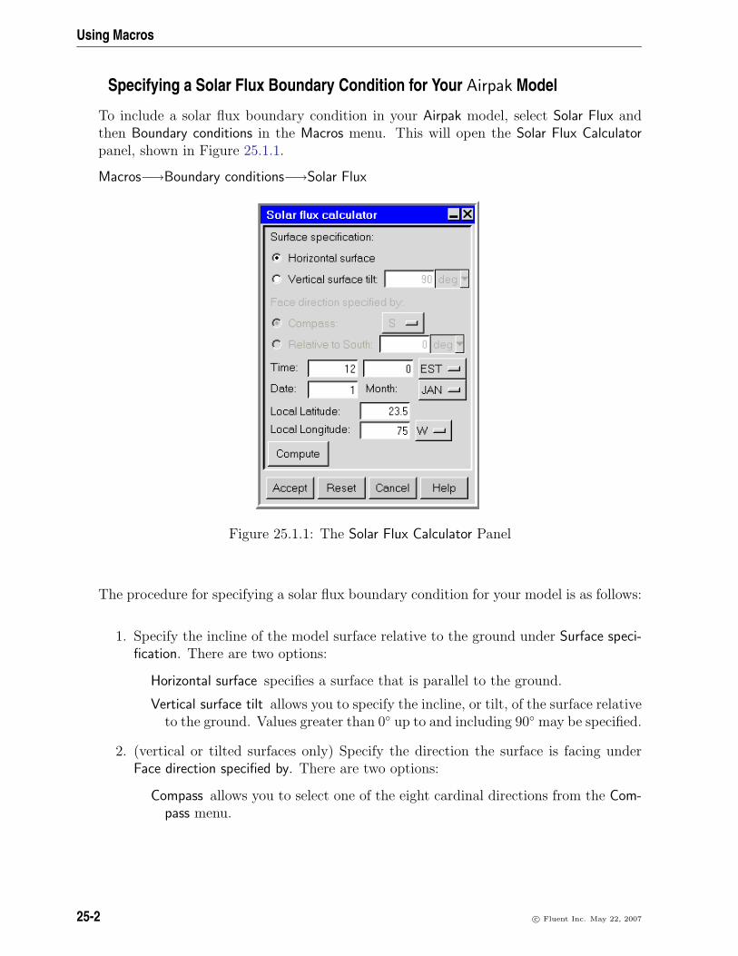
Using Macros
Specifying a Solar Flux Boundary Condition for Your Airpak Model
To include a solar flux boundary condition in your Airpak model, select Solar Flux andthen Boundary conditions in the Macros menu. This will open the Solar Flux Calculatorpanel, shown in Figure 25.1.1.
Macros−→Boundary conditions−→Solar Flux
Figure 25.1.1: The Solar Flux Calculator Panel
The procedure for specifying a solar flux boundary condition for your model is as follows:
1. Specify the incline of the model surface relative to the ground under Surface speci-fication. There are two options:
Horizontal surface specifies a surface that is parallel to the ground.
Vertical surface tilt allows you to specify the incline, or tilt, of the surface relativeto the ground. Values greater than 0 up to and including 90 may be specified.
2. (vertical or tilted surfaces only) Specify the direction the surface is facing underFace direction specified by. There are two options:
Compass allows you to select one of the eight cardinal directions from the Com-pass menu.
25-2 c© Fluent Inc. May 22, 2007
25.1 Boundary Condition Macros
Relative to South allows you to specify the surface face direction in degrees rel-ative to South. Values typically range from −180 to 180, where 0 is South,90 is West, −180 or 180 is North, and −90 is East.
3. Specify the local time at the desired location in the two fields to the right of Time.The time is based on a 24-hour clock, thus acceptable values range from 0 h 0 min(12:00 a.m.) to 23 h 59.99 min (11:59.99 p.m.). Values entered in the first text-entry field (hour) must be integral, but values entered in the second text-entry field(minute) can be integral or fractional. For example, if the local time was 12:01:30a.m., you would enter 0 for the hour and 1.5 for the minute. If the local time was4:17 p.m., you would enter 16 for the hour and 17 for the minute.
4. (optional) Specify the local time zone of the desired location using the menu to theright of the Time text-entry fields. The options are: Greenwich Mean Time (GMT),Atlantic Standard Time (AST), Eastern Standard Time (EST), Central StandardTime (CST), Mountain Standard Time (MST), and Pacific Standard Time (PST).The time zone is used to approximate the longitude (see below) of the location ifyou are unsure of the coordinates.
5. Specify the Date and Month of the year.
(a) Specify a value for the Date.
(b) Select the month from the Month menu.
6. Specify the Local Latitude of the desired location. Values can range from −90 (theSouth Pole) to 90 (the North Pole), with 0 defined as the equator.
7. Specify the Local Longitude of the desired location. The longitude is approximatedif you specify the local time zone, but you can enter a more precise value if youknow it. Any value you enter here will take precedence over the time zone. Valuesmay range from 0 to 180. Select the hemisphere (W or E) from the menu to theright of the Local Longitude text-entry field.
8. Click Compute to accept the parameters entered into the Solar Flux Calculator paneland calculate the solar irradiation flux boundary condition for your Airpak model.The Message window will display the following information:
• Local sunrise and sunset times
• Apparent solar time
• Direct (ED) and normal (EDN) components of the solar irradiation flux onthe surface in W/m2
• Diffuse sky radiation (Ed) in W/m2
• Total short-wave irradiance (Et = ED + Ed) in W/m2
For more information about these quantities and how they are calculated, see theASHRAE Fundamentals Handbook [1].
c© Fluent Inc. May 22, 2007 25-3

Using Macros
i If you click Compute in the Solar Flux Calculator panel after specifying animproper value for the date, time, latitude, or longitude, the Message windowwill inform you that a parameter is wrong. To fix an error, re-open the SolarFlux Calculator panel, adjust the parameter to an acceptable value, and clickCompute.
9. Specify the calculated heat flux as a boundary condition on the desired Airpak wallor block object. This step uses a wall object as an example.
Model−→Walls
(a) Create or select the desired wall object (see Section 13.7).
(b) In the Walls panel, specify an Outside heat flux equal to the total short-waveirradiance computed by the solar flux macro.
For example, at 7:00 a.m. on April 2 at 43.6 north latitude and 73.2 west longitude, thedirect component of the solar irradiation flux on a vertical wall facing west is calculatedto be 0 W/m2, and the diffuse sky radiation is calculated to be about 89 W/m2. Thereason that the direct component is 0 is that the outer surface of this particular wall ispointed away from the sun at 7:00 a.m.
At 4:00 p.m. on the same day, the direct component of the solar irradiation flux onthe wall is calculated to be about 610 W/m2 because the wall is now facing the sun.Combined with the calculated diffuse sky radiation of 532 W/m2, the total short-waveirradiance on the wall is about 1142 W/m2.
25.1.2 Atmospheric Boundary Layers
The atmospheric boundary layer macro allows you to characterize external wind flowsby the wind direction, wind speed, height above the ground, and a description of thelocal terrain. Using these parameters, Airpak can estimate the mean wind velocity at anyheight h using the following equations:
U(h) =
Umet
(dmet
Hmet
)amet(hd
)ah < d
Umet
(dmet
Hmet
)amet
h ≥ d
(25.1-1)
where
Umet = wind speed measured from a nearby meteorological stationHmet = anemometer heightamet = terrain factor for the meteorological stationdmet = boundary layer thickness at the meteorological stationa = terrain factor for desired locationd = boundary layer thickness at desired location
25-4 c© Fluent Inc. May 22, 2007

25.1 Boundary Condition Macros
In Equation 25.1-1, note that U(h) will remain constant at any height h equal to orgreater than the thickness of the boundary layer d.
The anemometer height is typically 10 m above ground level, withamet = 0.14 and dmet = 270 m, depending on the category of terrain surrounding themeteorological station. For the atmospheric boundary layer macro, you can characterizethe local terrain as one of the four types listed in Table 25.1.2 [1], or you can specify theterrain parameters yourself using your own knowledge or experience.
Table 25.1.1: Terrain Factor and Boundary Layer Thickness for Four Cate-gories of Land
Terrain Description a d (m)Category
1 Large city centers, in which at least 0.33 46050% of buildings are higher than 21 mover a distance of at least 2000 mupwind.
2 Urban, suburban, and wooded areas, 0.22 370and other areas with closely spacedobstructions compared to or largerthan single-family dwellings (over adistance of at least 2000 m upwind).
3 Open terrain with scattered obstacles 0.14 270generally less than 10 m high.
4 Flat, unobstructed areas exposed to 0.10 210wind flowing over a large body of water(no more than 500 m inland).
If one of the two-equation turbulence models (standard k-ε or RNG k-ε) is being used,the following boundary conditions will be applied to the atmospheric boundary layer:
• turbulent kinetic energy (constant)
k =(U∗)2√Cµ
(25.1-2)
• turbulent dissipation rate (varies with elevation)
ε =(U∗)3
κh(25.1-3)
c© Fluent Inc. May 22, 2007 25-5
Using Macros
where Cµ = 0.09, κ = 0.42 (von Karman’s constant), and
U∗ =κUmet
ln(Hmet
s)
(25.1-4)
where s is the roughness height.
From the above information, Airpak creates a rectangular opening with profiles to definethe wind velocity at various heights above the ground. The points in the profiles arecloser together nearer to the ground and more separated farther from the ground.
Once you have created the opening object, you may replace the turbulence boundaryconditions set by the macro with actual measured data if you are using one of the two-equation turbulence models (standard k-ε or RNG k-ε). See Section 11.4.1 for detailsabout turbulence profiles.
Adding an Atmospheric Boundary Layer to Your Airpak Model
Before you add an atmospheric boundary layer to your Airpak model, you will need tospecify the northward direction for your model in the Basic parameters panel. To openthe Basic parameters panel, doublle-click on the Basic parameters item under the Problemsetup node in the Model manager window.
Problem setup−→Basic parameters
Under Northward direction, specify values for (X, Y, Z) to define the northward directionfor your model. See Section 6.4.4 for more information about specifying the northwarddirection.
To include an atmospheric boundary layer in your Airpak model, select Boundary con-ditions and then Atmospheric boundary layer in the Macros menu. This will open theAtmospheric boundary layer panel, shown in Figure 25.1.2.
Macros−→Boundary conditions−→Atmospheric boundary layer
The procedure for adding an atmospheric boundary layer to your model is as follows:
1. Specify the position and size of the boundary layer.
(a) Specify the Plane in which the boundary layer lies (Y-Z, X-Z, or X-Y).
(b) Select Start/end and enter values for the start coordinates (xS, yS, zS) andend coordinates (xE, yE, zE, as appropriate) of the boundary layer, or selectStart/length and enter values for the start coordinates (xS, yS, zS) and thelengths of the sides (xL, yL, zL, as appropriate) of the boundary layer.
2. Specify the wind direction under Wind direction specified by.
There are two options:
25-6 c© Fluent Inc. May 22, 2007

25.1 Boundary Condition Macros
Figure 25.1.2: The Atmospheric boundary layer Panel
c© Fluent Inc. May 22, 2007 25-7
Using Macros
Compass allows you to select one of the eight cardinal directions from the Com-pass menu. The direction you select indicates from which direction the windis blowing.
Relative to North allows you to specify the wind direction in degrees relativeto the northward direction you specified in the Basic parameters panel (seeSection 6.4.4 for details). Values typically range from −180 to 180, where0 is North, 90 is East, −180 or 180 is South, and −90 is West. The valueyou enter indicates from which direction the wind is blowing.
Note that the wind direction you specify indicates from where the wind is blowing(e.g., from the North to the South). For example, if you define the positive x axis asthe northward direction in the Basic parameters panel and specify a wind directionof North in the Atmospheric boundary layer panel, the x-velocity magnitude will benegative, which indicates that the wind is blowing in the direction of the negativex axis.
3. Specify the Wind speed measured at the meteorological station (Umet in Equa-tion 25.1-1).
4. Specify the Anemometer height (Hmet in Equation 25.1-1). Typically, the windspeed is measured at 10 m above ground level.
5. (optional) Specify the Exponent (met), which is the terrain factor for the meteoro-logical station (amet in Equation 25.1-1). The default value of amet is 0.14, but youmay enter your own value for the terrain factor based on your own knowledge orexperience.
6. (optional) Specify the Boundary layer thickness (met) for the meteorological station(dmet in Equation 25.1-1). The default value of dmet is 270 m, but you may enteryour own value for the boundary layer thickness based on your own knowledge orexperience.
7. Select the Local terrain type. The four options (Large city centers; Urban, suburban,wooded areas; Scattered obstacles on open terrain; and Flat, unobstructed areas) aredescribed in Table 25.1.2.
8. (optional) Specify the Exponent, which is the terrain factor for the desired location(a in Equation 25.1-1). If your problem is not accurately modeled with one of thefour pre-defined terrain types, you can enter your own value for the terrain factorbased on your own knowledge or experience.
9. (optional) Specify the Boundary layer thickness for the desired location (d in Equa-tion 25.1-1). If your problem is not accurately modeled with one of the four pre-defined terrain types, you can enter your own value for the boundary layer thicknessbased on your own knowledge or experience.
25-8 c© Fluent Inc. May 22, 2007

25.1 Boundary Condition Macros
10. (two-equation turbulence models only) Specify the Surface roughness height for theproblem (s in Equation 25.1-4). By default, this value is set to 0.3 m. If yourproblem is not accurately described by this value, you can enter your own value forthe height of the roughness sublayer based on your own knowledge or experience.
11. Specify the Profile density, which is the number of points that will be included inthe velocity profile for the atmospheric boundary layer.
12. Specify the Profile direction. This is the direction in the Airpak model (X, Y, or Z,as available) in which the variation of height (h in Equation 25.1-1) is taking place,and should be perpendicular to the specified northward direction. See Section 6.4.4for more information about specifying the northward direction.
13. Specify whether you want the boundary layer to be available as one part or as anindividual object.
• If you want the boundary layer to be available as one part in your Airpakmodel, select Create internal part and specify a name in the Name text entryfield. The default name is blayer.n, where n is the next sequential numberamong numbered boundary layers.
• If you want the boundary layer to be available as an opening object, deselectCreate internal part. Airpak will create an opening with profiles to define thewind velocity at various heights above the ground.
14. If you want to save the current boundary layer specifications to be reused in yourcurrent model or to be used in a different model, click the Save button to openthe Macro information dialog box (which is the same as the File selection dialog boxdescribed in Section 2.1.8). Airpak will save the specifications in a subdirectorynamed blayer info.
To load boundary layer specifications that you have saved in this manner, click theLoad button and select the boundary layer specifications to be loaded.
15. Click Accept to accept the parameters entered into the Atmospheric boundary con-ditions panel and create the boundary layer.
Modifying an Existing Atmospheric Boundary Layer
After the boundary layer has been created and positioned in your Airpak model, it cannotbe modified using the Atmospheric boundary layer panel. There are two ways to modifyan existing boundary layer:
• If you selected the Create internal part option in the Atmospheric boundary layerpanel, you can edit the boundary layer in the same way that you edit a part (seeSection 7.8.5).
c© Fluent Inc. May 22, 2007 25-9

Using Macros
• If you did not select the Create internal part option in the Atmospheric boundary layerpanel, you must select and modify the opening object that makes up the boundarylayer.
25.2 Diffuser Macros
For simulations of room airflow, it is important to accurately model the behavior of airinlet diffusers and thus predict the penetration and spread of the air in the room. Thisperformance aspect of air inlet diffusers is referred to as the throw of the diffuser, which isdefined as the distance downstream of the diffuser where the jet centerline velocity equalsa specified terminal velocity. Due to the large scale differences between the dimensionsof the room and the important small geometrical features of diffusers, it is infeasiblecomputationally to explicitly model the detailed geometry of diffusers. Simply neglectingthe geometrical details of the diffuser usually leads to airflow simulations that deliver thecorrect amount of air into the room, but fail to achieve the proper jet penetration.However, simplified diffuser models that account for diffuser performance or the velocityfield in the vicinity of the diffuser exit can be used to predict the penetration and spreadof the air jet into the room. Airpak includes diffuser macros to help you accurately modelseveral different types of diffusers with simplified boundary conditions.
Information about modeling diffusers in Airpak is presented in the following sections:
• Section 25.2.1: Diffuser Modeling Methods
• Section 25.2.2: Diffuser Types
• Section 25.2.3: Steps for Adding a Diffuser to Your Airpak Model
• Section 25.2.5: Specifying Airflow Performance Data
• Section 25.2.4: Specifying Geometry, Position, and Size
• Section 25.2.6: Specifying the Extrusion and Flow Directions
• Section 25.2.7: Additional Inputs for Specific Types of Diffusers
• Section 25.2.8: Specifying Supply-Air and Room-Air Conditions
• Section 25.2.9: Specifying the Modeling Method
25.2.1 Diffuser Modeling Methods
The two primary methods for modeling diffusers with simplified boundary conditions [5]are the momentum method and the box method. These two methods are described below.
25-10 c© Fluent Inc. May 22, 2007

25.2 Diffuser Macros
Momentum Method
The momentum method assumes that the airflow from a particular diffuser can be pre-dicted using the isothermal axisymmetric jet formula
umu0
= K1
√A0
x(25.2-1)
where um is the centerline or maximum jet velocity at a distance x from the diffuser, u0
is the initial jet velocity, A0 is the effective area, and K1 is the empirically-determinedcenterline velocity decay constant. K1 may be a function of many factors, includingdiffuser type, Reynolds number, jet confinement, or possible deflections [1]. In airflowsimulations, the volumetric flow rate, Q, is specified and diffuser performance data pro-vide information on the throw x for a specific terminal velocity um and a given flow rateQ. Equation 25.2-1 can then be rearranged to solve for the initial jet velocity:
u0 =u2mx
2
K21Q
(25.2-2)
where Q = u0A0.
The initial jet velocity, u0, may be larger than the velocity, u, that is calculated by simplyusing the volumetric flow rate and the geometric area that the diffuser occupies (Ageom):
u =Q
Ageom
(25.2-3)
To properly model the diffuser performance, the simulation needs to ensure that theairflow from the diffuser enters the room with momentum corresponding to velocity u0
instead of momentum corresponding to velocity u. Typically, the diffuser is modeledwith a volumetric flow rate Q and a cross-sectional area Ageom. A momentum sourcethat accounts for u0 being the initial jet velocity is added to the diffuser to reproducediffuser performance in the simulation.
The same approach is used for linear jets; however, the implementation in Airpak forceiling diffusers (circular, square, and vortex) maintains the radial or lateral jet behaviorof the diffuser by modeling the circumferential distance of the diffuser and extruding thedirection normal to the ceiling until the modeled flow area equals the computed effectivearea.
Box Method
Although the momentum method works well for most types of diffusers, entrainmenteffects of discrete air jets from nozzle, linear slot, or valve diffusers are more accuratelymodeled using the box method.
c© Fluent Inc. May 22, 2007 25-11

Using Macros
The box method does not explicitly model the jet behavior in the immediate vicinityof the air inlet diffuser; instead, it specifies flow boundary conditions on the sides ofa rectangular region adjacent to the air inlet diffuser. For best accuracy with the boxmethod, velocity profiles from the inlet diffuser manufacturer or from measured datashould be used.
The box method in Airpak uses flat velocity profiles to account for entrainment effects,but you can improve the accuracy by supplying measured velocity profiles when you areediting the objects created by the diffuser macro
25.2.2 Diffuser Types
The following diffuser types are available in Airpak:
• Grille
• Ceiling
• Displacement
• Slot
• Nozzle
• Valve
• Vortex
Section 25.2.3 describes the steps for defining a diffuser in Airpak. See Figure 25.2.1 forgeneral information about inputs for each type of diffuser. Details about the inputs foreach type of diffuser are provided in Sections 25.2.5–25.2.9.
25.2.3 Steps for Adding a Diffuser to Your Airpak Model
To include a diffuser in your Airpak model, select Boundary conditions and then Diffuserin the Macros menu. This will open the Diffuser panel, shown for the different types ofdiffusers in Figures 25.2.2–25.2.14.
Macros−→Boundary conditions−→Diffuser
The procedure for adding a diffuser to your model is as follows:
1. Specify the Diffuser type by selecting Grille, Ceiling, Displacement, Slot, Nozzle, Valve,or Vortex. The panel will change (as shown in Figures 25.2.2–25.2.14) dependingon your selection of Diffuser type. Note that each Diffuser type panel has two tabs:Geometry and Properites.
25-12 c© Fluent Inc. May 22, 2007

25.2 Diffuser Macros
Figure 25.2.1: Diffuser Macro Flow Chart
c© Fluent Inc. May 22, 2007 25-13

Using Macros
2. Specify the geometry, position, and size of the diffuser. See Section 25.2.4 fordetails.
3. Specify the airflow performance data. See Section 25.2.5 for details.
4. Specify the extrusion direction and, if required, the flow direction for the diffuser.See Section 25.2.6 for details.
5. Specify any additional inputs that may be required for the diffuser. See Sec-tion 25.2.7 for details.
6. Specify the supply-air and room-air conditions. See Section 25.2.8 for details.
7. Select the method of modeling the diffuser, and specify the related parameters. SeeSection 25.2.9 for details.
8. Specify whether you want the diffuser to be available as one part or as individualobjects:
• If you want the diffuser to be available as one part in your Airpak model,select Create internal part and specify a name in the Name text entry field.The default name is diffuser.n, where n is the next sequential number amongnumbered diffusers.
• If you want the diffuser to be available as individual block, source, fan, oropening objects, deselect Create internal part. The individual Airpak objectsthat comprise the diffuser model will have the default name of type.n, wheretype is the type of diffuser and n is the next sequential number among num-bered Airpak objects. For example, if you create a rectangular grille diffuserusing the momentum method, Airpak will create a fan object called grille.1 anda source object called grille.2.
9. If you want to save the current diffuser specifications to be reused in your cur-rent model or to be used in a different model, click the Save button to open theMacro information dialog box (which is the same as the File selection dialog boxdescribed in Section 2.1.8). Airpak will save the specifications in a subdirectorynamed diffuser info.
To load diffuser specifications that you have saved in this manner, click the Loadbutton and select the diffuser specifications to be loaded.
10. Click Accept to accept the parameters entered into the Diffuser panel and createthe diffuser.
25-14 c© Fluent Inc. May 22, 2007

25.2 Diffuser Macros
i Objects created by the diffuser macro have hidden, performance-related informa-tion associated with the spatial location as defined in the Diffuser panel, and thusare not appropriate for copying or translating operations. To create several diffusersof similar geometry and performance, save the diffuser setup information and reuseit if you want to create a diffuser. The same restriction applies to running thediffuser at a different flow rate. Simply delete the previous diffuser and use thediffuser macro to create a new one.
i Objects created with the diffuser macro cannot be parameterized.
Modifying an Existing Diffuser
After the diffuser has been created and positioned in your Airpak model, it cannot bemodified using the Diffuser panel. There are two ways to modify an existing diffuser:
• If you selected the Create internal part option in the Diffuser panel, you can edit thediffuser in the same way that you edit a part (see Section 7.8.5).
• If you did not select the Create internal part option in the Diffuser panel, you mustselect and modify the object or objects that make up the diffuser.
c© Fluent Inc. May 22, 2007 25-15

Using Macros
Figure 25.2.2: The Grille Diffuser Panel (Geometry Tab)
25-16 c© Fluent Inc. May 22, 2007

25.2 Diffuser Macros
Figure 25.2.3: The Grille Diffuser Panel (Properties Tab)
c© Fluent Inc. May 22, 2007 25-17
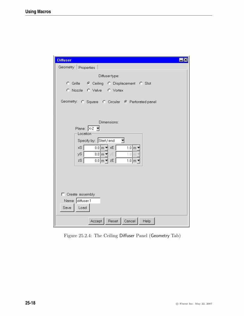
Using Macros
Figure 25.2.4: The Ceiling Diffuser Panel (Geometry Tab)
25-18 c© Fluent Inc. May 22, 2007

25.2 Diffuser Macros
Figure 25.2.5: The Ceiling Diffuser Panel (Properties Tab)
c© Fluent Inc. May 22, 2007 25-19

Using Macros
Figure 25.2.6: The Displacement Diffuser Panel (Geometry Tab)
25-20 c© Fluent Inc. May 22, 2007
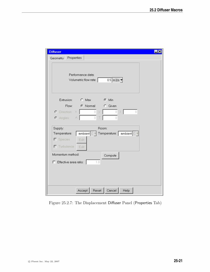
25.2 Diffuser Macros
Figure 25.2.7: The Displacement Diffuser Panel (Properties Tab)
c© Fluent Inc. May 22, 2007 25-21

Using Macros
Figure 25.2.8: The Slot Diffuser Panel (Geometry Tab)
25-22 c© Fluent Inc. May 22, 2007

25.2 Diffuser Macros
Figure 25.2.9: The Slot Diffuser Panel (Properties Tab)
c© Fluent Inc. May 22, 2007 25-23

Using Macros
Figure 25.2.10: The Nozzle Diffuser Panel (Geometry Tab)
25-24 c© Fluent Inc. May 22, 2007

25.2 Diffuser Macros
Figure 25.2.11: The Nozzle Diffuser Panel (Properties Tab)
c© Fluent Inc. May 22, 2007 25-25

Using Macros
Figure 25.2.12: The Valve Diffuser Panel (Geometry Tab)
25-26 c© Fluent Inc. May 22, 2007

25.2 Diffuser Macros
Figure 25.2.13: The Valve Diffuser Panel (Properties Tab)
c© Fluent Inc. May 22, 2007 25-27

Using Macros
Figure 25.2.14: The Vortex Diffuser Panel (Geometry Tab)
25-28 c© Fluent Inc. May 22, 2007

25.2 Diffuser Macros
Figure 25.2.15: The Vortex Diffuser Panel (Properties Tab)
c© Fluent Inc. May 22, 2007 25-29

Using Macros
25.2.4 Geometry, Position, and Size
The geometry types that are available will depend on which type of diffuser you areusing. See Figures 25.2.2–25.2.14 and below for details. The inputs for the standardAirpak geometries are described in Section 7.4.4. See Section 7.3.6 for details on resizingan object and Section 7.3.7 for details on repositioning an object. one
i Note that or the diffuser macro, there are two additional geometry types that youcan specify for a specific type of diffuser: square geometry and perforated panelgeometry. The inputs for both square and perforated panel geometry are similarto those of standard rectangular geometry. See Section 25.2.4 for details.
Information about the availability of each geometry type and how Airpak uses the infor-mation you provide for it is provided below.
Rectangular Geometry
Rectangular geometry is available for grille, displacement, and nozzle diffusers. De-pending on the modeling method you select (momentum or box), specifying rectangulargeometry will instruct Airpak to create different objects to represent your diffuser in themodel.
Momentum Method
If you select the momentum method, Airpak will create a 3D source object (four-sidedtop and bottom) with a rectangular fan object on the supply side. The height of thesource object is determined by the effective area of the diffuser (A0 in Equation 25.2-1),which is defined as
25-30 c© Fluent Inc. May 22, 2007
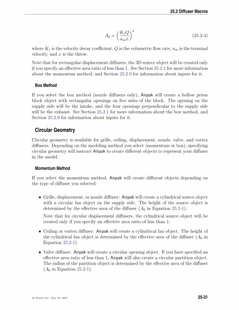
25.2 Diffuser Macros
A0 =(K1Q
umx
)2
(25.2-4)
where K1 is the velocity decay coefficient, Q is the volumetric flow rate, um is the terminalvelocity, and x is the throw.
Note that for rectangular displacement diffusers, the 3D source object will be created onlyif you specify an effective area ratio of less than 1. See Section 25.2.1 for more informationabout the momentum method, and Section 25.2.9 for information about inputs for it.
Box Method
If you select the box method (nozzle diffusers only), Airpak will create a hollow prismblock object with rectangular openings on five sides of the block. The opening on thesupply side will be the intake, and the four openings perpendicular to the supply sidewill be the exhaust. See Section 25.2.1 for more information about the box method, andSection 25.2.9 for information about inputs for it.
Circular Geometry
Circular geometry is available for grille, ceiling, displacement, nozzle, valve, and vortexdiffusers. Depending on the modeling method you select (momentum or box), specifyingcircular geometry will instruct Airpak to create different objects to represent your diffuserin the model.
Momentum Method
If you select the momentum method, Airpak will create different objects depending onthe type of diffuser you selected:
• Grille, displacement, or nozzle diffuser: Airpak will create a cylindrical source objectwith a circular fan object on the supply side. The height of the source object isdetermined by the effective area of the diffuser (A0 in Equation 25.2-1).
Note that for circular displacement diffusers, the cylindrical source object will becreated only if you specify an effective area ratio of less than 1.
• Ceiling or vortex diffuser: Airpak will create a cylindrical fan object. The height ofthe cylindrical fan object is determined by the effective area of the diffuser (A0 inEquation 25.2-1).
• Valve diffuser: Airpak will create a circular opening object. If you have specified aneffective area ratio of less than 1, Airpak will also create a circular partition object.The radius of the partition object is determined by the effective area of the diffuser(A0 in Equation 25.2-1).
c© Fluent Inc. May 22, 2007 25-31

Using Macros
See Section 25.2.1 for more information about the momentum method, and Section 25.2.9for information about inputs for it.
Box Method
If you select the box method (nozzle or valve diffusers only), Airpak will create a cylindricalblock object, a cylindrical fan object, and a circular opening object. The fan objectwill occupy the same space as the block object, with the block object acting as thesupport structure. The opening object will be on the supply side of the block object.See Section 25.2.1 for more information about the box method, and Section 25.2.9 forinformation about inputs for it.
Inclined Geometry
Inclined geometry is available for grille, displacement, and nozzle diffusers, for which youmust use the momentum method. Specifying inclined geometry will instruct Airpak tocreate a 3D source object (four-sided top and bottom) with an inclined rectangular fanobject on the supply side. The height of the source object is determined by the effectivearea of the diffuser (A0 in Equation 25.2-1).
Note that for inclined displacement diffusers, the 3D source object will be created only ifyou specify an effective area ratio of less than 1. See Section 25.2.1 for more informationabout the momentum method, and Section 25.2.9 for information about inputs for it.
Cylinder Geometry
Cylinder geometry is available for displacement diffusers, for which you must use themomentum method. Depending on the number of active corners you specify for thediffuser, specifying cylinder geometry will instruct Airpak to create different objects torepresent your diffuser in the model. See Section 25.2.7 for information about specifyingactive corners. See Section 25.2.1 for more information about the momentum method,and Section 25.2.9 for information about inputs for it.
Four Active Corners
If you specify the maximum of four active corners, Airpak will create a 3D fan object witha 16-sided top and bottom. If you have specified an effective area ratio of less than 1,Airpak will also create a 3D source object (four-sided top and bottom) on each of the16 equatorial sides of the fan. The height of the source objects is determined by theeffective area of the diffuser (A0 in Equation 25.2-1).
Less Than Four Active Corners
If you specify one, two, or three active corners, Airpak will create objects to representone, two, or three quarters of a cylinder. For each corner selected, Airpak will create a
25-32 c© Fluent Inc. May 22, 2007

25.2 Diffuser Macros
3D “pie piece” block object with four inclined rectangular fan objects on the four outersides of the block. If you have specified an effective area ratio of less than 1, Airpak willalso create a 3D source object (four-sided top and bottom) on the four outer sides of theblock. The height of the source objects is determined by the effective area of the diffuser(A0 in Equation 25.2-1).
Prism Geometry
Prism geometry is available for displacement diffusers, for which you must use the mo-mentum method. Specifying prism geometry will instruct Airpak to create a prism blockobject with a rectangular fan object on the supply side. If you have specified an effec-tive area ratio of less than 1, Airpak will also create a 3D source object (four-sided topand bottom) on the supply side. See Section 25.2.7 for information about specifyingthe supply side for prism geometry. See Section 25.2.1 for more information about themomentum method, and Section 25.2.9 for information about inputs for it.
Polygon Geometry
Polygon geometry is available for displacement diffusers, for which you must use themomentum method. Specifying polygon geometry will instruct Airpak to create a 3D fanobject with a top and bottom that have the number of vertices specified by you. If youhave specified an effective area ratio of less than 1, Airpak will also create a 3D sourceobject (four-sided top and bottom) on each equatorial side of the fan. The height of thesource objects is determined by the effective area of the diffuser (A0 in Equation 25.2-1).See Section 25.2.1 for more information about the momentum method, and Section 25.2.9for information about inputs for it.
Perforated Panel Geometry
Perforated panel geometry is available for ceiling diffusers, for which you must use themomentum method. Specifying perforated panel geometry will instruct Airpak to createa 3D source object (four-sided top and bottom) with a rectangular fan object on thesupply side. The height of the prism source object is determined by the effective area ofthe diffuser (A0 in Equation 25.2-1). See Section 25.2.1 for more information about themomentum method, and Section 25.2.9 for information about inputs for it.
Square Geometry
Square geometry is available for ceiling diffusers, for which you must use the momentummethod. Depending on the number of active sides you specify for the diffuser, specifyingsquare geometry will instruct Airpak to create different objects to represent your diffuserin the model. See Section 25.2.7 for information about specifying active sides. SeeSection 25.2.1 for more information about the momentum method, and Section 25.2.9for information about inputs for it.
c© Fluent Inc. May 22, 2007 25-33

Using Macros
Four Active Sides
If you specify the maximum of four active sides, Airpak will create a 3D polygon fanobject. The height of the polygon fan object is determined by the effective area of thediffuser (A0 in Equation 25.2-1).
Less Than Four Active Sides
If you specify one, two, or three active sides, Airpak will create a prism block object withrectangular intake fan objects on the specified active sides of the block object. The fanobjects will be perpendicular to the supply side of the block.
Linear Geometry
Linear geometry is available for slot diffusers. Depending on the modeling method youselect (momentum or box) and number of active sides you specify for the diffuser, spec-ifying linear geometry will instruct Airpak to create different objects to represent yourdiffuser in the model. See Section 25.2.7 for information about specifying active sides.See Section 25.2.1 for more information about the momentum method, and Section 25.2.9for information about inputs for it.
Momentum Method with Four Active Sides
If you select the momentum method and specify the maximum of four active sides, Airpakwill create a 3D polygon fan object. The height of the polygon fan object is determinedby the effective area of the diffuser (A0 in Equation 25.2-1).
Momentum Method with Less Than Four Active Sides
If you select the momentum method and specify one, two, or three active sides, Airpakwill create a prism block object with rectangular intake fan objects on the specified activesides of the block object. The fan objects will be perpendicular to the supply side of theblock.
Box Method
If you select the box method, Airpak will create a hollow prism block object with rect-angular openings on up to five sides of the block. The number of openings will dependon the number of active sides that you specify. The opening on the supply side will bethe exhaust, and the other openings perpendicular to the supply side will be the intake.See Section 25.2.1 for more information about the box method, and Section 25.2.9 forinformation about inputs for it.
25-34 c© Fluent Inc. May 22, 2007

25.2 Diffuser Macros
Vertical Geometry
Vertical geometry is available for slot diffusers. Depending on the modeling method youselect (momentum or box), specifying vertical geometry will instruct Airpak to createdifferent objects to represent your diffuser in the model.
Momentum Method
If you select the momentum method, Airpak will create a 3D source object (four-sidedtop and bottom) with a rectangular fan object on the supply side. The height of thesource object is determined by the effective area of the diffuser, A0, which is defined inEquation 25.2-4. The air flow will be delivered normal or at a specified angle to thesurface on which the diffuser is located. See Section 25.2.1 for more information aboutthe momentum method, and Section 25.2.9 for information about inputs for it.
Box Method
If you select the box method, Airpak will create a hollow prism block object with rect-angular openings on five sides of the block. The opening on the supply side will bethe intake, and the four openings perpendicular to the supply side will be the exhaust.See Section 25.2.1 for more information about the box method, and Section 25.2.9 forinformation about inputs for it.
clearpage
25.2.5 Specifying Airflow Performance Data
There are two ways you can specify performance data for the diffuser:
• Specify data for a single point.
• Specify a curve or curves.
i For displacement and valve diffusers, only the first method is available.
c© Fluent Inc. May 22, 2007 25-35

Using Macros
Specifying Performance Data for a Single Point
To specify performance data for a single point, select Performance data in the Diffuserpanel and specify the following values:
• Volumetric flow rate of air through the diffuser (Q in Equation 25.2-2)
• Terminal velocity (um in Equation 25.2-2) that corresponds to the air jet centerlinevelocity value for which the throw is specified
• Throw distance of the air jet from the diffuser (x in Equation 25.2-2) at which theair jet centerline velocity equals the specified terminal velocity
Note that, for displacement and valve diffusers, only the volumetric flow rate is specified.
Specifying Performance Curves
To specify performance data for a series of points, select Performance curves in the Dif-fuser panel. For grille, ceiling, slot, nozzle, and vortex diffusers, you can define up tothree curves using the Performance data panel (Figure 25.2.16). As noted above, thisspecification method is not available for displacement and valve diffusers.
The procedure for defining a performance curve is as follows:
1. Specify the number of the curve (1, 2, or 3) in the drop-down list above the Editbutton.
2. Click Edit to open the Performance data panel.
3. Specify a list of values in the Performance data panel. A curve specification consistsof a list of volumetric flow rate/throw sets, with one volumetric flow rate value andone throw value in each set. It is important to give the numbers in sets of two,but the spacing between numbers is not important. The sets must be entered inorder of increasing volumetric flow rate so that the data can be interpolated whenrequired.
4. Specify the Terminal velocity that corresponds to the air jet centerline velocity valuefor which the throw is desired. The throw distance of an air jet is a function of thevolumetric flow rate for a particular terminal velocity.
5. Select the appropriate Volumetric flow rate units for your listed values from the unitdefinition list.
6. Select the appropriate Throw units for your listed values from the unit definitionlist.
25-36 c© Fluent Inc. May 22, 2007

25.2 Diffuser Macros
Figure 25.2.16: The Performance data Panel
7. Click Accept. This will store the values and close the Performance data panel. Airpakwill interpolate the data you provided for the volumetric flow rate and the throwto create a profile for the diffuser.
8. Click Edit in the Diffuser panel to re-open the Performance data panel.
9. In the Performance data panel, specify the Volumetric flow rate for the diffuser.
10. Click Compute throw to compute the throw distance value for the diffuser basedon the performance curve. In the Diffuser panel, a set of Performance data will beupdated (Volumetric flow rate, Terminal velocity, and Throw). The Message windowwill also print this information.
Loading a Previously Defined Curve
To load a previously defined profile, click on Load. (See Section 28.2.8 for details onsaving contour data and using them as a profile.) This will open the Load curve file
c© Fluent Inc. May 22, 2007 25-37

Using Macros
selection dialog box. Select the file containing the profile data and click Accept. SeeSection 2.1.8 for details on selecting a file. If you know the units used in the profile datayou are loading, you should select the appropriate units in the Performance data panelbefore you load the profile.
Saving a Curve
To save a profile, click on Save. This will open the Save curve dialog box, in which youcan specify the filename and directory to which the profile data are to be saved.
25.2.6 Specifying the Extrusion and Flow Directions
Specifying the Extrusion Direction
For all diffuser types, you will need to specify the direction of the Extrusion. For 3Ddiffusers, the height, or extrusion, is usually calculated using the effective area (A0 inEquation 25.2-1). The extrusion direction is the direction in which the Airpak objectsare extended. Depending on the location of the diffuser in the room, you need to makesure that the diffuser is extruded into the room volume and not out of the room volume.
There are two options for the Extrusion direction:
Max specifies that the extrusion points in the direction of increasing coordinate value.For example, if you have positioned a grille diffuser on a surface on the x-y planewith the positive z direction pointing into the room, you should select Max.
Min specifies that the extrusion points in the direction of decreasing coordinate value.For example, if you have positioned a grille diffuser on a surface on the x-z planewith the negative y direction pointing into the room, you should select Min.
Note that you will not specify the extrusion direction in this way for a cylindrical dis-placement diffuser. See Section 25.2.7 for details.
25-38 c© Fluent Inc. May 22, 2007

25.2 Diffuser Macros
Specifying the Flow Direction
If you are modeling grille, slot, nozzle, or certain types of ceiling (perforated panel ge-ometry) or displacement (rectangular, circular, or inclined geometry) diffusers, you willneed to specify the Flow direction. There are two options:
• If the air flows into the room normal to the diffuser, select Normal.
• To specify the flow angle of the fluid entering the room through the diffuser, selectGiven. There are two specification methods:
Direction allows you to specify the direction vector (x, y, z) for the flow. Onlythe direction of the vector is used by Airpak; the magnitude is ignored.
Angles allows you to specify the direction of the flow entering the room in termsof angles relative to the inward-pointing normal direction. You can specifytwo angles, A (α) and T (θ), to account for incoming flow not aligned with thenormal direction. If the normal inward vector points in the positive direction,then α and θ must have values in the range −90 < angle < 90, with α=θ=0
representing flow in the positive normal direction. If the normal inward vectorpoints in the negative direction, then α and θ must have values in the range90 < angle < 270, with α=θ=180 representing flow in the negative normaldirection. Since the diffuser may be oriented in any one of three planes (x-y,y-z, or x-z), the roles of α and θ will vary depending on the orientation of theplane of the diffuser.
If you are modeling valve, vortex, or certain types of ceiling (square geometry) or displace-ment (cylindrical or prism geometry) diffusers, you will use other methods to specify theflow direction. See Section 25.2.7 for details. If you are modeling polygon displacementdiffusers or circular ceiling diffusers, the flow direction will be normal to the diffuser.
25.2.7 Additional Inputs for Specific Types of Diffusers
For specific types of diffusers, there are additional inputs that are required in the Diffuserpanel. These special inputs are described below.
Specifying Active Corners for a Cylindrical Displacement Diffuser
If you have selected cylindrical geometry for a displacement diffuser, you must specifythe active Corners of the diffuser. You must specify a minimum of one active corner andmay specify up to four. Depending on the plane you selected for the diffuser, the fourcorner options (+ +, − +, − −, + −) will represent the four quadrants of a completecylinder with its center at the location that you have specified.
c© Fluent Inc. May 22, 2007 25-39
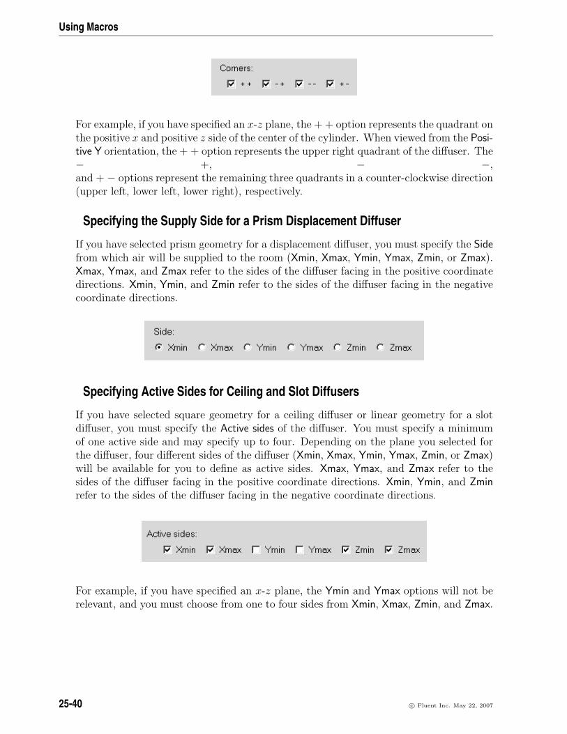
Using Macros
For example, if you have specified an x-z plane, the + + option represents the quadrant onthe positive x and positive z side of the center of the cylinder. When viewed from the Posi-tive Y orientation, the + + option represents the upper right quadrant of the diffuser. The− +, − −,and + − options represent the remaining three quadrants in a counter-clockwise direction(upper left, lower left, lower right), respectively.
Specifying the Supply Side for a Prism Displacement Diffuser
If you have selected prism geometry for a displacement diffuser, you must specify the Sidefrom which air will be supplied to the room (Xmin, Xmax, Ymin, Ymax, Zmin, or Zmax).Xmax, Ymax, and Zmax refer to the sides of the diffuser facing in the positive coordinatedirections. Xmin, Ymin, and Zmin refer to the sides of the diffuser facing in the negativecoordinate directions.
Specifying Active Sides for Ceiling and Slot Diffusers
If you have selected square geometry for a ceiling diffuser or linear geometry for a slotdiffuser, you must specify the Active sides of the diffuser. You must specify a minimumof one active side and may specify up to four. Depending on the plane you selected forthe diffuser, four different sides of the diffuser (Xmin, Xmax, Ymin, Ymax, Zmin, or Zmax)will be available for you to define as active sides. Xmax, Ymax, and Zmax refer to thesides of the diffuser facing in the positive coordinate directions. Xmin, Ymin, and Zminrefer to the sides of the diffuser facing in the negative coordinate directions.
For example, if you have specified an x-z plane, the Ymin and Ymax options will not berelevant, and you must choose from one to four sides from Xmin, Xmax, Zmin, and Zmax.
25-40 c© Fluent Inc. May 22, 2007

25.2 Diffuser Macros
Special Inputs for Valve and Vortex Diffusers
If you have selected a valve diffuser, you will need to specify the Jet cone angle insteadof the flow direction.
If you have selected a vortex diffuser, you will need to specify the Swirl angle instead ofthe flow direction.
25.2.8 Specifying Supply-Air and Room-Air Conditions
Specifying Supply-Air and Room-Air Temperatures
For all diffuser types, Airpak calculates a local Archimedes number (Ar) to give an indica-tion of the relative importance of buoyant forces. For Airpak to calculate the local valueof Ar, you will need to estimate the temperatures of both the supply air and the roomair. Specify the temperature of the supply air in the Temperature field under Supply, andthe temperature of the room air in the Temperature field under Room.
Specifying Supply-Air Species Parameters
If you have enabled the Species option in the Problem setup panel, you can specify speciesparameters for the diffuser supply air using the Supply species concentration panel (Fig-ure 25.2.17). To open the Supply species concentration panel, select the Species option inthe Diffuser panel and click Edit.
Figure 25.2.17: The Supply species concentration Panel
See Chapter 21 for details on modeling species transport.
c© Fluent Inc. May 22, 2007 25-41

Using Macros
Specifying Supply-Air Turbulence Parameters
If you selected the two-equation or RNG k-ε model in the Basic parameters panel, you canspecify turbulence parameters for the diffuser supply air using the Turbulence equationparameters panel (Figure 25.2.18). To open the Turbulence equation parameters panel,select Turbulence in the Diffuser panel and click Edit.
Figure 25.2.18: The Turbulence equation parameters Panel
Specify the Turbulent intensity as a percentage, and the Turbulent length scale in theappropriate units of length. See Section 6.4.3 for details on determining turbulenceparameters.
25.2.9 Specifying the Modeling Method
For all diffuser types, you will need to select the method of modeling the diffuser. SeeSection 25.2.1 for more information about diffuser modeling methods.
There are two methods of modeling diffusers in Airpak.
Momentum method specifies the momentum method for modeling the diffuser. Thisoption is available for all diffuser types, and is recommended for grille, ceiling,displacement, and vortex diffusers. See Section 25.2.4 for details about the types ofAirpak objects that are created when you choose the momentum method for specificdiffusers. See below for information about input options for the momentum method.
Box method specifies the box method for modeling the diffuser. This option is avail-able and recommended for slot, nozzle, and valve diffusers. See Section 25.2.4 fordetails about the types of Airpak objects that are created when you choose the boxmethod for specific diffusers. See below for information about input options for thebox method.
Inputs for the Momentum Method
The default approach in the momentum method is to use jet theory and published cor-relations to determine the effective area. You can modify this approach in several ways:
25-42 c© Fluent Inc. May 22, 2007

25.2 Diffuser Macros
• Specify that corrections be applied
• Specify parameters that are used in the correlations for some diffusers
• Specify aspects of the diffuser performance that you want to control yourself
The options for controlling the momentum method are as follows:
Attached jet correction specifies a correction factor for the default value of K1. Thisoption is available for grille diffusers and accounts for jets from high side-walldiffusers attached to the ceiling.
Velocity decay constant directly specifies a value for K1 that overrides the default valueof the velocity decay constant. This option is available for grille, ceiling, slot, nozzle,and vortex diffusers.
Variable constant calculates a value for K1 based on the estimated discharge velocity.This option is available only for slot diffusers with linear geometry.
Effective area ratio directly specifies the ratio of the effective area (A0 in Equation 25.2-1)to the total area of the diffuser. This option is available for grille, displacement,slot, nozzle, and valve diffusers. Specifying the effective area ratio, which can besupplied by the diffuser manufacturer or obtained from your own diffuser perfor-mance measurements, allows you to bypass calculating the effective area based onjet theory and correlations.
Free area ratio directly specifies the free area ratio, which is a parameter in correlationsfor the velocity decay constant K1 for grille and perforated-panel ceiling diffusers.
The Compute button instructs Airpak to calculate values for various parameters anddisplay them in the Message window. These parameters include the discharge velocity,effective area, Archimedes number, and others that depend on the momentum methodoptions you have selected.
c© Fluent Inc. May 22, 2007 25-43

Using Macros
Figure 25.2.19: The Box method parameters Panel
Inputs for the Box Method
You can specify parameters for the box method using the Box method parameters panel(Figure 25.2.19). To open the Box method parameters panel for a slot, nozzle, or valvediffuser, select the Box method option in the Diffuser panel and click Edit.
The procedure for specifying box method parameters for your diffuser is as follows:
1. For rectangular diffusers, enter values for the lengths of the sides (xL, yL, zL) of thebox under Box geometry type. For circular diffusers, enter values for the Height andRadius of the “box”.
2. Click the Check box button to check whether the box dimensions are large enoughto adequately model the diffuser.
i The Archimedes number (Ar) cannot be 0 if you are using the box method. Ifyou get an Error dialog box, click OK and adjust either the room temperature orthe supply air temperature so that they are different values. See Section 25.2.8for details.
The Message window will inform you if your box dimensions are too small or toolarge. Once you have specified adequate box dimensions, click Check box and theMessage window will display Check OK.
25-44 c© Fluent Inc. May 22, 2007

25.3 Geometry Macros
3. Specify the Entrainment factor, which is the ratio of the volumetric flow rate of theair jet relative to the volumetric flow rate of air exiting the diffuser.
4. If you have enabled the Species option in the Problem setup panel, you can specifyspecies parameters for the diffuser exhaust air using the Exhaust species concentra-tion panel (Figure 25.2.20). To open the Exhaust species concentration panel, selectSpecies in the Box method parameters panel and click Edit.
Figure 25.2.20: The Exhaust species concentration Panel
See Chapter 21 for details on modeling species transport.
5. Click the Compute Tbox & Cbox button to compute the temperature and, if required,the mass fraction of species that exit the box. This accounts for mixing betweenthe supply air and the entrained room air. The Message window will display valuesfor Tbox (temperature) and Cbox (mass fraction).
6. Click Accept in the Box method parameters panel.
25.3 Geometry Macros
The following geometry-related macros are described in this section:
• Section 25.3.1: Polygonal Ducts
• Section 25.3.3: Closed Box
• Section 25.3.4: 1/4 Polygonal Cylinder
• Section 25.3.5: Cylinder Plates
• Section 25.3.6: Cylindrical Enclosure
• Section 25.3.7: Polygonal Circle
• Section 25.3.8: Polygonal Cylinder
• Section 25.3.9: Hemisphere
c© Fluent Inc. May 22, 2007 25-45

Using Macros
25.3.1 Polygonal Ducts
Polygonal ducts are created using wire objects (described in Chapter 19). At least threewires are necessary to construct a polygonal duct. The number of walls (sides) of theduct is equal to the number of wires used in its construction. The macro uses the non-uniform polygonal block object with a zero height to construct the walls (sides) of theduct from the wires.
25.3.2 Adding a Polygonal Duct to Your Airpak Model
To include a polygonal duct in your Airpak model, select Quick geometry/approximationsand then Polygonal ducts in the Macros menu. This will open the Polygonal ducts panel,shown in Figure 25.3.1.
Macros−→Quick geometry/approximations−→Polygonal ducts
Once you have created the wires that will be used to construct the polygonal duct, theprocedure for adding a polygonal duct to your model is as follows:
1. Select the wires to be used to create the polygonal duct in the Available list. Thenames of the wires that will be used will be displayed in the Used list.
2. If you want to close the duct at the starting end, select Close starting end.
3. If you want to close the duct at the finishing end, select Close finishing end.
4. If you want the polygonal duct to be available as an assembly in your Airpak model,select Create assembly. If you want the polygonal duct to be available as individualobjects, deselect Create assembly. The individual block elements that comprise thewalls (sides) of the polygonal duct will be created with the default name duct.n,where n is the next sequential number among numbered block objects in the duct.
5. If you have created an assembly and want to change the name of the polygonal duct,enter a new name in the Name text entry field. The default name is polyduct.n,where n is the next sequential number among numbered polygonal ducts.
6. Click Accept to accept the parameters entered into the Polygonal ducts panel andcreate the polygonal duct.
Modifying an Existing Polygonal Duct
After the polygonal duct has been created and positioned in your Airpak model, it cannotbe modified using the Polygonal ducts panel. There are two ways to modify an existingpolygonal duct:
25-46 c© Fluent Inc. May 22, 2007

25.3 Geometry Macros
Figure 25.3.1: The Polygonal ducts Panel
c© Fluent Inc. May 22, 2007 25-47

Using Macros
• If you selected the Create assembly option in the Polygonal ducts panel, you can editthe polygonal duct in the same way that you edit an assembly (see Section 7.8.5).
• If you did not select the Create assembly option in the Polygonal ducts panel, youmust individually select and modify the polygonal duct’s block objects.
25.3.3 Closed Box
The closed box macro allows you to enclose spaces in your Airpak model and assignproperties to the sides of the enclosure. Two types of enclosures can be created usingthe closed box macro:
• A box that encloses the whole room with six Airpak wall objects
• A box that encloses part of the room with six Airpak partition objects
The closed box macro can be used to reduce the number of steps required to create thesix individual sides of an enclosure.
Adding a Closed Box to Your Airpak Model
To include a closed box in your Airpak model, select Quick geometry/approximations andthen Closed box in the Macros menu. This will open the Closed Box panel, shown inFigure 25.3.2.
Macros−→Quick geometry/approximations−→Closed Box
The procedure for adding a closed box to your model is as follows:
1. Select Start/end and enter values for the start coordinates (xS, yS, zS) and endcoordinates (xE, yE, zE) of the box, or select Start/length and enter values for thestart coordinates (xS, yS, zS) and the lengths of the sides (xL, yL, zL) of the box.
2. Specify whether the box is Internal (encloses part of the room) or External (enclosesthe whole room) next to Box type.
3. If the thickness of the box sides is to be non-zero, select Thick walls. For zero-thickness box sides, deselect Thick walls.
4. (non-zero-thickness box sides only) Specify the Thickness of the box sides. Whenthe thickness of the sides of an internal box is non-zero, the heat flow through thesides is based on the conductivity of the sides. For non-zero-thickness sides on anexternal box, the heat flow is computed based on the conductivity of the sides,the computed temperature on the inner surfaces of the sides, and the conditionsapplied at the outer surfaces of the sides.
25-48 c© Fluent Inc. May 22, 2007

25.3 Geometry Macros
Figure 25.3.2: The Closed Box Panel
c© Fluent Inc. May 22, 2007 25-49

Using Macros
If the thickness is non-zero, each side is expanded inward or outward from the planeof the side. If the thickness is positive, the sides are expanded to the specifiedthickness in the positive direction of the coordinate axis that is normal to the planeof each side. If the thickness is specified with a negative sign, the expansion is inthe negative direction of the coordinate axis normal to the plane of each side.
5. (non-zero-thickness box sides only) If you specify a non-zero thickness for the sidesof the box, you must also specify the Box material for the sides. The selectionof default means that the material specified as the Box material is defined underDefault solid in the Basic parameters panel (see Section 6.4.7). To change the Boxmaterial for the sides, select a material from the Box material drop-down list. SeeSection 7.7 for details on material properties.
6. (external box sides only) Specify the External material for the sides of the box.The selection of default means that the material specified as the External materialfor the sides is defined under Default surface in the Basic parameters panel (seeSection 6.4.7). To change the External material for the sides, select a material fromthe External material drop-down list. The surface roughness and emissivity aredefined as part of the surface material parameters. You can edit these values if youselect Edit definition in the materials list. See Section 7.7 for details on materialproperties.
7. (external, non-zero-thickness box sides only) If you specify a non-zero thicknessfor external box sides, you also need to specify the Internal material for the sides.The selection of default means that the material specified as the Internal materialfor the sides is defined under Default surface in the Basic parameters panel (see Sec-tion 6.4.7). To change the Internal material for the sides, select a material from theInternal material drop-down list. The surface roughness and emissivity are defined aspart of the surface material parameters. You can edit these values if you select Editdefinition in the materials list. See Section 7.7 for details on material properties.
8. Specify whether you want the box to be available as one part or as individualobjects.
• If you want the box to be available as one part in your Airpak model, selectCreate assembly and specify a name in the Name text entry field. The defaultname is box.n, where n is the next sequential number among numbered boxes.
• If you want the box to be available as individual wall or partition objects,deselect Create assembly. Airpak will create six partition objects for an Internalbox (one for each side of the box) or six wall objects for an External box (torepresent the floor, ceiling, and sides of the room).
9. If you want to save the current box specifications to be reused in your currentmodel or to be used in a different model, click the Save button to open the Macroinformation dialog box (which is the same as the File selection dialog box described inSection 2.1.8). Airpak will save the specifications in a subdirectory named box info.
25-50 c© Fluent Inc. May 22, 2007

25.3 Geometry Macros
To load box specifications that you have saved in this manner, click the Load buttonand select the box specifications to be loaded.
10. Click Accept to accept the parameters entered into the Closed Box panel and createthe box.
Modifying an Existing Closed Box
After the box has been created and positioned in your Airpak model, it cannot be modifiedusing the Closed Box panel. There are two ways to modify an existing box:
• If you selected the Create assembly option in the Closed Box panel, you can edit thebox in the same way that you edit a part (see Section 7.8.5).
• If you did not select the Create assembly option in theClosed Box panel, you must individually select and modify the wall or partitionobjects that make up the box.
25.3.4 1/4 Polygonal Cylinder
The 1/4 polygonal cylinder macro can be used to create a 1/4 polygonal representationof a cylinder for the following object types:
• Blocks
• Sources
• Resistances
Facets for the total number to be used are specified, and the number must be an evennumber.
Adding a Polygonal Cylinder to Your Airpak Model
To include a 1/4 polygonal cylinder in your Airpak model, select Quick geometry/approximationsand then 1/4 Polygonal cylinder in the Macros menu. This will open the Polygonal cylinderpanel, shown in Figure 25.3.3.
Macros−→Quick geometry/approximations−→1/4 Polygonal cylinder
The procedure for adding a 1/4 polygonal cylinder to your model is as follows:
1. Specify the Dimensions of the polygonal enclosure. Enter the values of the startcoordinates (xC, yC, zC), Radius and the Length of the cylinder.
c© Fluent Inc. May 22, 2007 25-51

Using Macros
Figure 25.3.3: The 1/4 Polygonal cylinder Panel
25-52 c© Fluent Inc. May 22, 2007

25.3 Geometry Macros
2. Select the Plane of the polygonal cylinder (YZ, XZ, or XY).
3. Select the Quadrants to be created. You can choose to create any or all of the fourquadrants of the cylinder. All four quadrants are created as separate geometries.
4. Specify the total number of Facets as an even number.
5. Select the Object Type that will be created (Block, Source, or Resistance).
Modifying an Existing 1/4 Polygonal Cylinder
After the 1/4 polygonal cylinder has been created and positioned in your Airpak model,it cannot be modified using the Polygonal cylinder panel. There are two ways to modifyan existing polygonal cylinder:
• If you selected the Create assembly option in the Polygonal cylinder panel, you canedit the box in the same way that you edit a part (see Section 7.8.5).
• If you did not select the Create assembly option in thePolygonal cylinder panel, you must individually select and modify the wall or parti-tion objects that make up the polygonal cylinder.
25.3.5 Cylinder Plate
The cylinder plate macro allows you to create a cylindrical representation of a plate inyour Airpak model by faceting the surface of a cylinder with thin conducting plates. Thefacets are specified per quarter and must be even in number.
Adding a Cylinder Plate to Your Airpak Model
To include a cylindrical plate in your Airpak model, select Quick geometry/approximationsand then Cylinder plates in the Macros menu. This will open the Cylinder plates panel,shown in Figure 25.3.4.
Macros−→Quick geometry/approximations−→Cylinder plates
The procedure for adding a cylinder plate to your model is as follows:
1. Specify the Dimensions of the cylinder plate. Enter the values of the start coordi-nates (xC, yC, zC), the Radius of the circle, and the Length of the plate.
2. Specify whether the polygon will be created Inside (polygon touches the edge of thebounding circle) or Outside (polygon is tangent to the edge of the inner circle).
3. Select the Axis of the polygon (X, Y, or Z).
4. Specify the Facets per Quarter as an even number.
c© Fluent Inc. May 22, 2007 25-53

Using Macros
Figure 25.3.4: The Cylinder plates Panel
25-54 c© Fluent Inc. May 22, 2007

25.3 Geometry Macros
Modifying an Existing Cylinder Plate
After the cylinder plate has been created and positioned in your Airpak model, it cannotbe modified using the Cylinder Plate panel. There are two ways to modify an existingbox:
• If you selected the Create assembly option in the Cylinder plates panel, you can editthe box in the same way that you edit a part (see Section 7.8.5).
• If you did not select the Create assembly option in theCylinder plates panel, you must individually select and modify the wall or parti-tion objects that make up the cylinder plate.
25.3.6 Cylindrical Enclosure
This macro allows you to create a cylindrical enclosure for your Airpak model. Thisenclosure consists of four hollow polygonal blocks that change the shape of the room intoa cylinder. Walls are then used to facet the sides of the polygonal blocks in contact withthe fluid and the remaining sections of the room. Facets are per quarter, and must beeven in number.
Adding a Cylindrical Enclosure to Your Airpak Model
To include a cylindrical enclosure in your Airpak model, select Quick geometry/approximationsand then Cylindrical enclosure in the Macros menu. This will open the Cylindrical enclosurepanel, shown in Figure 25.3.5.
Macros−→Quick geometry/approximations−→Cylindrical enclosure
The procedure for adding a cylindrical enclosure to your model is as follows:
1. Specify the Dimensions of the cylindrical enclosure. Enter the values of the startcoordinates (xC, yC, zC), the Radius of the circle, and the Length of the plate.
2. Specify whether the polygon will be created Inside (polygon touches the edge of thebounding circle) or Outside (polygon is tangent to the edge of the inner circle).
3. Specify whether the polygon will be sized to the dimension of the room or not byselecting Yes or No, respectively, for Size Room.
4. Select the Axis of the polygon (X, Y, or Z).
5. Specify the Facets per Quarter as an even number.
c© Fluent Inc. May 22, 2007 25-55

Using Macros
Figure 25.3.5: The Cylindrical enclosure Panel
25-56 c© Fluent Inc. May 22, 2007

25.3 Geometry Macros
Figure 25.3.6: A Cylindrical Enclosure with 16 Facets and 4 Corners
c© Fluent Inc. May 22, 2007 25-57
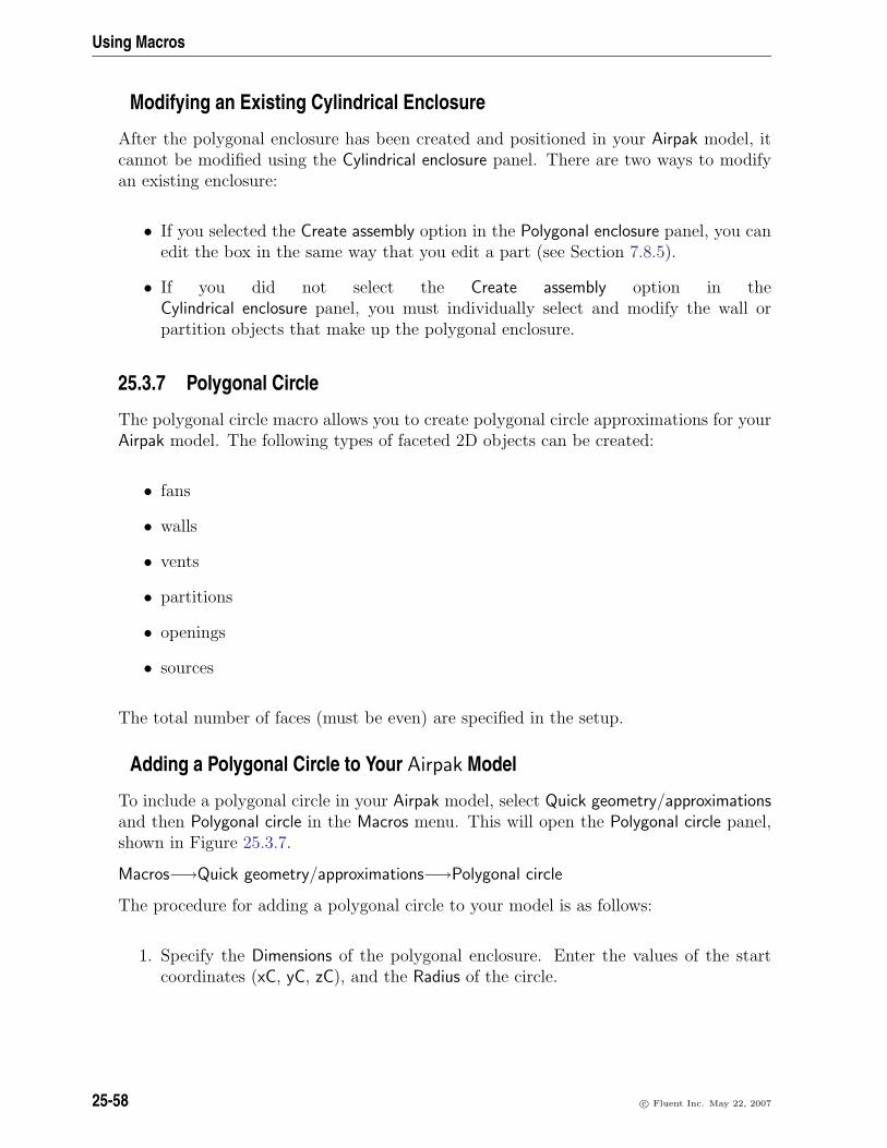
Using Macros
Modifying an Existing Cylindrical Enclosure
After the polygonal enclosure has been created and positioned in your Airpak model, itcannot be modified using the Cylindrical enclosure panel. There are two ways to modifyan existing enclosure:
• If you selected the Create assembly option in the Polygonal enclosure panel, you canedit the box in the same way that you edit a part (see Section 7.8.5).
• If you did not select the Create assembly option in theCylindrical enclosure panel, you must individually select and modify the wall orpartition objects that make up the polygonal enclosure.
25.3.7 Polygonal Circle
The polygonal circle macro allows you to create polygonal circle approximations for yourAirpak model. The following types of faceted 2D objects can be created:
• fans
• walls
• vents
• partitions
• openings
• sources
The total number of faces (must be even) are specified in the setup.
Adding a Polygonal Circle to Your Airpak Model
To include a polygonal circle in your Airpak model, select Quick geometry/approximationsand then Polygonal circle in the Macros menu. This will open the Polygonal circle panel,shown in Figure 25.3.7.
Macros−→Quick geometry/approximations−→Polygonal circle
The procedure for adding a polygonal circle to your model is as follows:
1. Specify the Dimensions of the polygonal enclosure. Enter the values of the startcoordinates (xC, yC, zC), and the Radius of the circle.
25-58 c© Fluent Inc. May 22, 2007

25.3 Geometry Macros
Figure 25.3.7: The Polygonal circle Panel
c© Fluent Inc. May 22, 2007 25-59

Using Macros
2. Specify whether the radius will be used as the Outer surface (polygon is tangent tothe edge of the inner circle) or the Inner surface (polygon touches the edge of thebounding circle).
3. Select the Plane of the polygonal circle (YZ, XZ, or XY).
4. Specify the Facets per Quarter as an even number.
5. Select the Object Type that will be created (Fan, Vent. Opening, Wall, Partition, orSource.
Modifying an Existing Polygonal Circle
After the polygonal circle has been created and positioned in your Airpak model, it cannotbe modified using the Polygonal circle panel. There are two ways to modify an existingpolygonal circle:
• If you selected the Create assembly option in the Polygonal circle panel, you can editthe box in the same way that you edit a part (see Section 7.8.5).
• If you did not select the Create assembly option in thePolygonal circle panel, you must individually select and modify the wall or par-tition objects that make up the polygonal circle.
25.3.8 Polygonal Cylinder
The polygonal cylinder macro can be used to create a polygonal representation of acylinder for the following object types:
• Blocks
• Sources
• Resistances
Facets for the total number to be used are specified, and the number must be an evennumber.
25-60 c© Fluent Inc. May 22, 2007

25.3 Geometry Macros
Figure 25.3.8: The Polygonal cylinder Panel
c© Fluent Inc. May 22, 2007 25-61

Using Macros
Adding a Polygonal Cylinder to Your Airpak Model
To include a polygonal cylinder in your Airpak model, select Quick geometry/approximationsand then Polygonal cylinder in the Macros menu. This will open the Polygonal cylinderpanel, shown in Figure 25.3.8.
Macros−→Quick geometry/approximations−→Polygonal cylinder
The procedure for adding a polygonal cylinder to your model is as follows:
1. Specify the Dimensions of the polygonal enclosure. Enter the values of the startcoordinates (xC, yC, zC), and the Outer radius of the circle.
2. Specify whether the radius will be used as the Outside surface (polygon is tangentto the edge of the inner circle) or the Inside surface (polygon touches the edge ofthe bounding circle).
3. Specify the Length of the cylinder.
4. Select the Plane of the polygonal cylinder (YZ, XZ, or XY).
5. Specify the total number of Facets as an even number.
6. Select the Object Type that will be created (Block, Source, or Resistance).
Modifying an Existing Polygonal Cylinder
After the polygonal cylinder has been created and positioned in your Airpak model, itcannot be modified using the Polygonal cylinder panel. There are two ways to modify anexisting polygonal cylinder:
• If you selected the Create assembly option in the Polygonal cylinder panel, you canedit the box in the same way that you edit a part (see Section 7.8.5).
• If you did not select the Create assembly option in thePolygonal cylinder panel, you must individually select and modify the wall or parti-tion objects that make up the polygonal cylinder.
25.3.9 Hemisphere
The hemisphere macro can be used to create a layered representation of a hemispherecomprised of stacked non-uniform cylinders. You have the ability to use any of themeshing options with this macro, as opposed to using true hemisphere geometry whichwould restrict usage to only the tetrahedral mesher.
25-62 c© Fluent Inc. May 22, 2007

25.3 Geometry Macros
Adding a Hemisphere to Your Airpak Model
To include a hemisphere in your Airpak model, select Quick geometry/approximations andthen Hemisphere in the Macros menu. This will open the Hemisphere panel, shown inFigure 25.3.9.
Macros−→Quick geometry/approximations−→Hemisphere
Figure 25.3.9: The Hemisphere Panel
The procedure for adding a hemisphere to your model is as follows:
1. Specify the Dimensions of the polygonal enclosure. Enter the values of the start
c© Fluent Inc. May 22, 2007 25-63

Using Macros
coordinates (xC, yC, zC), and the Radius of the circle.
2. Specify whether the radius will be used as the Outside surface (polygon is tangentto the edge of the inner circle) or the Inside surface (polygon touches the edge ofthe bounding circle).
3. Select the Plane of the hemisphere (YZ, XZ, or XY).
4. Select the Direction of the hemisphere (Low, High, or Both). The Direction refersto whether the hemisphere will be created advancing out from the high side of thespecified plane that contains the center of the hemisphere, or from the low side ofthat specified plane.
5. Specify the Number of steps which is the number of non-uniform cylinder layers touse in forming the hemisphere.
6. Select the Method (Height or Angle) to be used to create the hemisphere. The Heightoption will create layer which are uniform in height. Alternatively, the Angle optionwill create layers that vary in height but represent uniform increments of angle tothe center of the hemisphere for each layer.
Modifying an Existing Hemisphere
After the hemisphere has been created and positioned in your Airpak model, it cannot bemodified using the Hemisphere panel. There are two ways to modify an hemisphere:
• If you selected the Create assembly option in the Hemisphere panel, you can edit thebox in the same way that you edit a part (see Section 7.8.5).
• If you did not select the Create assembly option in theHemisphere panel, you must individually select and modify the wall or partitionobjects that make up the hemisphere.
25-64 c© Fluent Inc. May 22, 2007

25.4 Object Rotation Macros
25.4 Object Rotation Macros
The following object rotation macros are described in this section:
• Section 25.4.1: Rotating Plates
• Section 25.4.2: Rotating Prismatic Blocks
• Section 25.4.3: Rotating Polygonal Blocks
• Section 25.4.4: Rotating Groups of Prismatic Blocks
25.4.1 Rotating Individual Plates
This macro allows you to create a polygonal block that represents an individual rotatedplate in your Airpak model. You can rotate an individual plate about either a givenpoint, its centroid, or a particular edge through an arbitrary angle and given coordinateaxis. Where multiple plates are selected, the centroid/edge that you specify is for theindividual plate, and not for the bounding box of the combined selection. Airpak thengenerates an inclined plane to represent the rotated plate.
Adding a Rotated Individual Plate to Your Airpak Model
To rotate an individual plate and add it to your Airpak model, select Rotate objects andthen Individual plates in the Macros menu. This will open the Rotate prism plates panel,shown in Figure 25.4.1.
Macros−→Rotate objects−→Individual plates
The procedure for rotating an individual plate and adding it to your model is as follows:
1. Select the Axis of rotation (X, Y, or Z).
2. Specify the Angle of rotation.
3. Select Pivot about location of the plate as either a given point (Point), its centroid(Centroid), or a particular edge through an arbitrary angle and given coordinate(Vertex).
4. Specify the centroid coordinate of the plate (x0 and y0).
5. Specify whether to use the list of all Available partitions in the model for the rotationoperation, or Used which is a list of selected partitions.
6. Click Accept.
c© Fluent Inc. May 22, 2007 25-65

Using Macros
Figure 25.4.1: The Rotate prism plates Panel
25-66 c© Fluent Inc. May 22, 2007

25.4 Object Rotation Macros
25.4.2 Rotating Prismatic Blocks
This macro allows you to create a polygonal block that represents an individual rotatedprismatic block in your Airpak model. You can rotate a prism block about either a givenpoint, its centroid, or a particular edge through an arbitrary angle and given coordinateaxis. Where multiple plates are selected, the centroid/edge that you specify is for theindividual prism block, and not for the bounding box of the combined selection. Airpakgenerates a polygonal block that is the representation of the rotated prism block.
Adding a Rotated Prismatic Block to Your Airpak Model
To rotate an individual prism block and add it to your Airpak model, select Rotate objectsand then /Individual Prism blocks in the Macros menu. This will open the Rotate prismblocks panel, shown in Figure 25.4.2.
Macros−→Rotate objects−→Individual prism blocks
Figure 25.4.2: The Rotate prism blocks Panel
The procedure for rotating a prism block and adding it to your model is as follows:
c© Fluent Inc. May 22, 2007 25-67

Using Macros
1. Select the Axis of rotation (X, Y, or Z).
2. Specify the Angle of rotation.
3. Select Pivot about method as either a given point (Point), its centroid (Centroid),or a particular edge through an arbitrary angle and given coordinate (Vertex).
4. Specify the centroid coordinate (x0 and y0).
5. Specify whether to use the list of all Available partitions in the model for the rotationoperation, or Used which is a list of selected partitions.
6. Click Accept.
25.4.3 Rotating Polygonal Blocks
This macro allows you to create a polygonal block that represents an individual rotatedpolygonal block in your Airpak model. You can rotate a polygonal block about eithera given point, its centroid, or a particular edge through an arbitrary angle and givencoordinate axis. Where multiple plates are selected, the centroid/edge that you specifyis for the individual polygonal block, and not for the bounding box of the combinedselection. Airpak generates a polygonal block that is the representation of the rotatedprism block.
Adding a Rotated Polygonal Block to Your Airpak Model
To rotate an individual polygonal block and add it to your Airpak model, select Rotateobjects and then Individual polygonal blocks in the Macros menu. This will open the Rotatepolygonal blocks panel, shown in Figure 25.4.3.
Macros−→Rotate objects−→Individual polygonal blocks
The procedure for rotating a polygonal block and adding it to your model is as follows:
1. Specify the Angle of rotation.
2. Select Pivot about coordinate (guixP, yP, and zP).
3. Specify whether to use the list of all Available partitions in the model for the rotationoperation, or Used which is a list of selected partitions.
4. Click Accept.
25-68 c© Fluent Inc. May 22, 2007

25.4 Object Rotation Macros
Figure 25.4.3: The Rotate polygonal blocks Panel
c© Fluent Inc. May 22, 2007 25-69

Using Macros
25.4.4 Rotating Groups of Prismatic Blocks
This macro allows you to create a polygonal block that represents an individual rotatedpolygonal block in your Airpak model. You can rotate a polygonal block about eithera given point, its centroid, or a particular edge through an arbitrary angle and givencoordinate axis. Where multiple plates are selected, the centroid/edge that you specifyis for the individual polygonal block, and not for the bounding box of the combinedselection. Airpak generates a polygonal block that is the representation of the rotatedprism block.
Adding a Rotated Group of Prism Blocks to Your Airpak Model
To rotate a group of prismatic blocks and add it to your Airpak model, select Rotateobjects and then Groups of prism blocks in the Macros menu. This will open the Rotategroup of prism blocks panel, shown in Figure 25.4.4.
Macros−→Rotate objects−→Groups of prism blocks
Figure 25.4.4: The Rotate groups of prism blocks Panel
The procedure for rotating a group of prism blocks and adding it to your model is asfollows:
25-70 c© Fluent Inc. May 22, 2007

25.4 Object Rotation Macros
1. Select the Axis of rotation (X, Y, or Z).
2. Specify the Angle of rotation.
3. Select the Pivot Point coordinate (x0 and y0).
4. Specify whether to use the list of all Available partitions in the model for the rotationoperation, or Used which is a list of selected partitions.
5. Click Accept.
c© Fluent Inc. May 22, 2007 25-71

Using Macros
25-72 c© Fluent Inc. May 22, 2007

Chapter 26. Generating a Mesh
This chapter provides information about generating a computational mesh for your Airpakmodel.
• Section 26.1: Overview
• Section 26.2: Mesh Quality and Type
• Section 26.3: Guidelines for Mesh Generation
• Section 26.4: Creating a Minimum-Count Mesh
• Section 26.5: Refining the Mesh Globally
• Section 26.6: Refining the Mesh Locally
• Section 26.7: Controlling the Meshing Order for Objects
• Section 26.8: Non-Conformal Meshing Procedures for Assemblies
• Section 26.9: Displaying the Mesh
• Section 26.10: Checking the Mesh
• Section 26.11: Exporting a Mesh
• Section 26.12: Loading an Existing Mesh
26.1 Overview
Once you have finished designing your model, you need to generate the computationalmesh that is used as the basis of the solution procedure. The mesh consists of discreteelements located throughout the computational domain. Within each element, Airpaksolves the equations that govern the flow and heat transfer in the room.
A good computational mesh is an essential ingredient for a successful and accurate solu-tion. If the overall mesh is too coarse, the resulting solution may be inaccurate. If theoverall mesh is too fine, the computational cost may become prohibitive. In summary,the cost and accuracy of the solution are directly dependent on the quality of the mesh.
Airpak automates the mesh generation procedure, but allows you to customize the mesh-ing parameters in order to refine the mesh and optimize trade-offs between computational
c© Fluent Inc. May 22, 2007 26-1

Generating a Mesh
cost and solution accuracy. You can apply such modified parameters at a global level(affecting the entire computational domain) or to specific modeling objects. This flexi-bility provides you with an efficient mesh generation process that you can influence asmuch (or as little) as you want.
The meshing procedure that Airpak follows is based on a set of rules that govern how eachtype of object is to be meshed. Airpak operates on a “cocooning” methodology wherebyeach object is meshed individually, as tightly as your specifications permit, in orderto resolve the physics of the solution optimally. In every case, optimal resolution of thephysics depends on the specific problem to be solved. The mesh elements are smaller nearobjects (as shown in Figure 26.1.1), to take into account thermal and velocity gradientsthat are often present near the boundaries of an object. By contrast, the open spacesbetween objects are meshed with large elements, to minimize computational costs.
Figure 26.1.1: Mesh with Small Elements Near Objects and Large Elementsin Open Spaces
26-2 c© Fluent Inc. May 22, 2007

26.2 Mesh Quality and Type
26.2 Mesh Quality and Type
26.2.1 Mesh Quality
As mentioned in Section 26.1, the quality of the mesh is one of the most critical aspectsof a CFD model. A good mesh is essential for a good solution. A good mesh requiresproper resolution, smoothness, low skewness, and an appropriate number of elements.The main requirements can be summarized as follows:
• The mesh must be fine near objects where the gradients of temperature and ve-locity may be very large (e.g., heated blocks or partitions, room walls with nearbyobjects). See Figure 26.1.1 for an example.
• The expansion ratio from one mesh element to the next should be kept in the rangebetween 2 and 5, although in some critical areas a lower value might be better.The mesh in Figure 26.1.1 shows good expansion ratios.
• An equilateral element (cube or equilateral tetrahedron) is optimal. Since it isgenerally not possible to have only optimal elements, you should instead focus onmaintaining a low aspect ratio and regular (not skewed) shape for each element.This will reduce the number of long, thin elements and the number of distortedelements, both of which can decrease accuracy and destabilize the solution. Fig-ure 26.2.1 shows examples of elements with low and high skew.
Figure 26.2.1: Elements with Low and High Skew
• It is also possible to have non-conformal meshing in a certain region of the modelto improve grid quality and/or to reduce the mesh count. A bounding box canbe applied to a certain region, and the mesh inside this region need not match themesh outside the region. One disadvantage of this method is that currently, particletraces cannot cross the boundaries of a non-conformal interface. See Section 28.2.10for more information on particle traces.
• For an efficient calculation, the mesh should be coarser in areas where the gradientsof velocity and temperature are small. Since there are no small changes in flow
c© Fluent Inc. May 22, 2007 26-3

Generating a Mesh
behavior to be captured, it would be wasteful to have a fine mesh in such regions.The cost of the calculation will be directly proportional to the number of elementsin the mesh, so it is best to concentrate the elements where you need them, andreduce the number of elements elsewhere.
26.2.2 Hexahedral, Tetrahedral and Hex-Dominant Meshes
There are three types of meshers available in Airpak: hexahedral, tetrahedral and hex-dominant. The hexahedral unstructured mesher (the default) is appropriate for mostapplications. For geometrically complicated models that include, for example, sphericalor ellipsoidal objects, the tetrahedral mesher will generally produce a better mesh thanthe hexahedral mesher. In fact, the tetrahedral mesher is required if your model includesellipsoids, elliptical cylinders, or polygonal ducts. The hex-dominant mesher can be usedfor automatic meshing of CAD geometries. Hex-dominant is a robust and highly auto-mated unstructured mesh generator that can handle grids of virtually unlimited size andcomplexity, consisting mostly of hexahedral elements but including triangular, tetrahe-dral or pyramidal cells. The hex-dominant mesher uses advanced meshing algorithms toallow the most appropriate cell type to be used to generate body-fitted meshes for themost general CAD geometries. Additionally, an Airpak hexahedral mesh can be gener-ated as Cartesian or unstructured. The hexahedral Cartesian mesher can create betterquality cells for some simple problems, but may not approximate geometry that is ei-ther curved or not aligned with the model axes, as well as the unstructured hexahedralmesher. The Cartesian mesher will turn off O-grid type meshes around objects, and willuse stair-stepping to approximate inclined and curved faces. It is generally recommendedto use the Hexa unstructured mesher (the default option). The same controls that areused for the automatic unstructured hexahedral mesher (the default mesher) will be avail-able for you to create a Cartesian mesh. Additionally, the controls for the hexahedraland hex-dominant meshers are the same. Hence, for information on the procedures forhex-dominant meshing, refer to the section on hexahedral meshing, Section 26.3.1. SeeSection 26.3.2 for information on the procedures for tetrahedral meshing.
26.3 Guidelines for Mesh Generation
For best results, mesh generation should be an iterative procedure. Guidelines for ap-proaching mesh generation are presented in this section, and specific instructions forthe procedures mentioned here are provided in the sections that follow. The hexahedralmeshing procedure, which should be used for most applications, is presented in Sec-tion 26.3.1. These procedures are valid for the hex-dominant mesher as well. Proceduresfor using the optional tetrahedral mesher are presented in Section 26.3.2.
i The tetrahedral mesher should be used only when you are meshing very complexgeometric shapes (i.e., when there are objects present in the model that cannot be
26-4 c© Fluent Inc. May 22, 2007

26.3 Guidelines for Mesh Generation
meshed with the hexahedral mesher, or if the hexahedral mesher fails to producean acceptable grid). Furthermore, the use of the tetrahedral mesher with manyobjects that have very small dimensions (such as partitions with a small thickness)can lead to very large meshes. Objects for which the tetrahedral mesher must beused include ellipsoids, elliptical cylinders, and polygonal ducts.
26.3.1 Hexahedral Meshing Procedure
The recommended approach to hexahedral mesh generation is as follows:
1. Generate a mesh using Airpak’s default parameters for a coarse mesh (see Sec-tion 26.4.1), using the default Hexa unstructured mesher. The resulting mesh (calledthe minimum-count mesh) contains the minimum number of elements required toadequately represent the model geometry and satisfy the default meshing rules.
You can compute an approximate solution on this initial mesh to determine quicklyif the calculation runs properly and the results seem reasonable, before proceedingto refine the mesh and compute a more accurate solution. This initial calculationwill also allow you to estimate the total computation cost.
2. Generate a refined mesh.
(a) Set the Max X size, Max Y size, and Max Z size values to about 1/20 of theroom dimensions in the corresponding directions.
(b) Select the Normal mesh resolution.
(c) Generate the mesh.
See Section 26.5.1 for details.
3. Examine the mesh, using plane cuts and diagnostics (as described in Sections 26.9and 26.10), to see if it satisfies the following requirements:
• The number of elements between solid faces should be at least 2.
• There should be at least 4 or 5 elements on each flow object (openings, vents,resistances, fans).
• The mesh quality should satisfy the requirements outlined in Section 26.2.
4. If the mesh does not satisfy these requirements, use the object-specific meshingcontrols to refine the mesh locally and improve the mesh quality. Suggestions arelisted below:
• Refine the mesh around objects where the temperature and velocity gradientsare expected to be high (e.g., heated blocks and partitions, objects blockingor diverting the flow, fans).
c© Fluent Inc. May 22, 2007 26-5

Generating a Mesh
• If the element count on the face of an object is low, use the X, Y, or Z count(or the corresponding parameter) to change it.
• Use high and low element size and ratio to refine the mesh around objects.You can also use the inward/outward size and ratio to refine the mesh.
See Section 26.6 for details.
Additional options for improving the mesh are as follows:
• If your model includes a small number of objects, and the element count orspacing on all of them is low, you can use the Init height option to turn onO-grid cocooning (Hexa unstructured mesher only) and place graded elementson the faces of all objects. This option should be used only when the numberof objects is not too large; otherwise, the mesh count can become very large.See Section 26.5.1 for details.
• In some cases, setting the Max O-grid height to a small enough value relativeto the object size will yield better mesh quality by localizing the cocooningaction of the mesher. Note that the value of Max O-grid height should behigher than that of Init height, and that a value of 0 for Max O-grid heightleaves the O-grid height unbounded. See Section 26.5.1 for details.
• Aligning faces that are nearly aligned (see Figure 26.3.1) will generally reducethe overall mesh size and result in better convergence (due to the improvedaspect ratio of the elements). You can align faces by modifying the coordinatesof the appropriate object(s), or by using the alignment tools (see Section 2.1.3).
Figure 26.3.1: Aligning Nearly-Aligned Faces
• Rectangular objects are generally easier to mesh than circular objects. Insome cases, you may be able to improve the mesh quality without affecting thesolution by replacing circular objects (fans, openings, etc.) with rectangularobjects of the same type. For models with circular objects you may also wantto consider using the tetrahedral mesher (described in Section 26.3.2) insteadof the hexahedral mesher.
• You can use fluid blocks to refine or otherwise improve the mesh locally. Unlessyou change their material properties, fluid blocks do not alter the flow ortemperature distribution inside the room because they are, by default, madeof air, which is the material inside the rest of the room as well.
5. Calculate a solution on the refined mesh.
26-6 c© Fluent Inc. May 22, 2007

26.3 Guidelines for Mesh Generation
6. For optimal accuracy, refine the mesh further, calculate a solution, and compareit with the solution for the previous mesh. Repeat until the solution is grid-independent (i.e., until it no longer changes with each new mesh).
26.3.2 Tetrahedral Meshing Procedure
As mentioned in Section 26.3, the tetrahedral mesher should be used only when you aremeshing very complex geometric shapes, i.e., when there are objects present in the modelthat cannot be meshed with the hexahedral mesher, or if the hexahedral mesher fails toproduce an acceptable grid.
The recommended approach to tetrahedral mesh generation is as follows:
1. Generate a coarse mesh by turning off the Max tetra size criterion (see Section 26.4.2for details). The resulting mesh (called the minimum-count mesh) contains theminimum number of elements required to adequately represent the model geometryand satisfy the default meshing rules.
You can compute an approximate solution on this initial mesh to determine quicklyif the calculation runs properly and the results seem reasonable, before proceedingto refine the mesh and compute a more accurate solution. This initial calculationwill also allow you to estimate the total computation cost.
2. Generate a refined mesh.
(a) Turn on the Max tetra size option and specify the desired maximum lengthof an element’s side. A typical value is about 1/20 of the smallest roomdimension.
(b) Generate the mesh.
See Section 26.5.2 for details.
3. Examine the mesh, using plane cuts and diagnostics (as described in Sections 26.9and 26.10), to see if it satisfies the following requirements:
• The number of elements between solid faces should be at least 2.
• There should be at least 4 or 5 elements on each flow object (openings, vents,resistances, fans).
• The mesh quality should satisfy the requirements outlined in Section 26.2.
4. If the mesh does not satisfy these requirements, use the object-specific meshingcontrols to refine the mesh locally and improve the mesh quality. Suggestions arelisted below:
• Refine the mesh around objects where the temperature and velocity gradientsare expected to be high (e.g., heated blocks and partitions, objects blockingor diverting the flow, fans).
c© Fluent Inc. May 22, 2007 26-7

Generating a Mesh
• Use high and low element size to refine the mesh around objects. You can alsouse the inward/outward size to refine the mesh.
See Section 26.6 for details.
Additional options for improving the mesh are as follows:
• Reduce the Max tetra size if many of the elements are too large. This optionshould be used with caution, since it can cause the mesh count to become verylarge.
• Aligning faces that are nearly aligned (see Figure 26.3.1) will generally reducethe overall mesh size and result in better convergence (due to the low aspectratio of the elements). You can align faces by modifying the coordinates ofthe appropriate object(s).
• You can use fluid blocks to refine or otherwise improve the mesh locally. Unlessyou change their material properties, fluid blocks do not alter the flow ortemperature distribution inside the room because they are, by default, madeof air, which is the material inside the rest of the room as well.
5. Calculate a solution on the refined mesh.
6. For optimal accuracy, refine the mesh further, calculate a solution, and compareit with the solution for the previous mesh. Repeat until the solution is grid-independent (i.e., until it no longer changes with each new mesh).
26.4 Creating a Minimum-Count Mesh
As discussed in Sections 26.3.1 and 26.3.2, the minimum-count mesh is useful for com-puting an initial solution. Airpak generates a minimum-count mesh using the minimumnumber of elements necessary to represent the geometry and satisfy the default meshingrules for the objects in your model.
26.4.1 Creating a Minimum-Count Hexahedral Mesh
The steps you should follow to create a minimum-count hexahedral mesh for your modelare listed below:
1. Open the Mesh control panel (Figure 26.4.1) by selecting Generate mesh in the Model
menu, or by clicking on the button in the Model and solve toolbar.
Model−→Generate mesh
2. Click on the Generate tab (the default when the panel is opened for the first time)to access the controls for mesh generation. Keep the default selection of Hexaunstructured for the Mesh type.
26-8 c© Fluent Inc. May 22, 2007

26.4 Creating a Minimum-Count Mesh
Figure 26.4.1: The Mesh control Panel for the Hexahedral Mesher
3. Select Coarse in the Mesh parameters drop-down list to update the panel with thedefault settings for a coarse mesh.
4. Click Generate mesh. Airpak will generate the minimum-count mesh, which you canview as described in Section 26.9. If you want to stop the meshing process beforeit is complete, click Terminate mesher.
As discussed in Section 26.3.1, you will generally want to refine the minimum-count meshafter computing an initial solution. Airpak provides several parameters for refining themesh globally (i.e., throughout the entire computational domain) and locally (i.e., on ornear individual objects in the model). See Sections 26.5 and 26.6 for details.
c© Fluent Inc. May 22, 2007 26-9

Generating a Mesh
26.4.2 Creating a Minimum-Count Tetrahedral Mesh
The steps you should follow to create a minimum-count tetrahedral mesh for your modelare listed below:
1. Open the Mesh control panel (Figure 26.4.2) by selecting Generate mesh in the Model
menu, or by clicking on the button in the Model and solve toolbar.
Model−→Generate mesh
Figure 26.4.2: The Mesh control Panel for the Tetrahedral Mesher
2. Click on the Generate tab (the default when the panel is opened for the first time)to access the controls for mesh generation.
3. Select Tetra in the Mesh type drop-down list.
26-10 c© Fluent Inc. May 22, 2007

26.5 Refining the Mesh Globally
4. Turn off the Max tetra size option.
5. Click Generate mesh. Airpak will generate the minimum-count mesh, which you canview as described in Section 26.9. If you want to stop the meshing process beforeit is complete, click Terminate mesher.
As discussed in Section 26.3.2, you will generally want to refine the minimum-count meshafter computing an initial solution. Airpak provides several parameters for refining themesh globally (i.e., throughout the entire computational domain) and locally (i.e., on ornear individual objects in the model). See Sections 26.5 and 26.6 for details.
26.5 Refining the Mesh Globally
As discussed in Sections 26.3.1 and 26.3.2, you will generally want to refine the minimum-count mesh after computing an initial solution. The steps you should follow to refine themesh globally (i.e., throughout the entire computational domain) are presented here forboth hexahedral and tetrahedral meshes. See Section 26.6 for information about refiningthe mesh on or near individual objects in the model.
26.5.1 Global Refinement for a Hexahedral Mesh
The procedure for globally refining a hexahedral mesh is as follows:
1. Open the Mesh control panel (Figure 26.4.1) by selecting Generate mesh in the Model
menu, or by clicking on the button in the Model and solve toolbar.
Model−→Generate mesh
2. Click on the Generate tab to access the controls for mesh generation.
3. Select Hexa unstructured (the default mesher) in the Mesh type drop-down list.
4. Turn on the Max X size, Max Y size, and Max Z size specifications, and set eachone to the desired maximum element length in each direction. Typical values areabout 1/20 of the room dimensions in the corresponding directions.
5. (only for models with a small number of objects) To increase the number of elementson or near all objects, and reduce the mesh spacing on or near all objects, turn onthe Init height option and specify a value.
The Init height specifies the maximum height of the first element layer generated onthe surface of any modeling object (e.g., PCB, block, or fan). By default, Airpakuses its own internal rules to determine the height of the first element on the surfaceof an object (the initial height).
c© Fluent Inc. May 22, 2007 26-11

Generating a Mesh
i This option should be used only when the number of objects is not too large;otherwise, the mesh count can become very large.
6. Next to Minimum gap, specify the minimum distances separating objects in yourmodel in the X, Y, and Z coordinate directions.
This specification is used by Airpak whenever the distance between two objects isless than this value, but greater than the model’s zero tolerance. If the minimumgap specified for any of the three coordinate directions is more than the size ofthe smallest object in that coordinate direction, Airpak will display a Minimumseparation warning. You can let Airpak determine the appropriate minimum gapby clicking the Change value and mesh in the Minimum separation warning panel.You can choose to let Airpak automatically set appropriate minimum gap valueswithout using the Minimum separation warning panel by selecting Accept ”changevalue” checks in the Mesh control panel.
7. In the Mesh parameters drop-down list, select Normal to update the panel with thedefault settings for a normal, non-coarse mesh. If you want, you can modify thedefault settings, which are defined as follows:
Min elems in gap specifies the minimum number of elements between adjacentobjects.
Min elems on edge specifies the minimum number of elements on each edge ofeach object.
Max size ratio specifies the maximum ratio of the sizes of adjacent elements (forthe whole model).
Max O-grid height (Hexa unstructured mesher only) specifies the distance of thecocooning from the surface of the object (see Figure 26.5.1).
Figure 26.5.1: O-Grid Height
26-12 c© Fluent Inc. May 22, 2007

26.5 Refining the Mesh Globally
Min elems on cyl face specifies the minimum number of elements on the circularface of a cylindrical object (e.g., a cylindrical block). If you consider the mesharound the cylinder to be box-like, this is the minimum number of intervalson each edge of the box.
Min elems on tri face specifies the minimum number of elements on the triangu-lar face of an object (e.g., a polygonal block with a triangular face). If youconsider the mesh around the triangle to be box-like, this is the minimumnumber of intervals on each edge of the box.
Cylinder shrink factor specifies the factor of adjustment for diameters of cylindri-cal shapes in cases where the cylinder touches other surfaces tangentially atits side surface.
Max elements specifies the maximum number of elements in the mesh.
No O-grids (Hexa unstructured mesher only) indicates whether or not objects willhave O-grids around them. This option is off by default, indicating that Airpakwill put O-grids around all objects, including those that contain other objects.
No group O-grids (Hexa unstructured mesher only) indicates whether or not ob-jects with other objects inside them (e.g., an enclosure that has blocks insideit) will have O-grids around them. This option is off by default, indicatingthat Airpak will put O-grids around all objects, including those that containother objects.
Mesh assemblies separately indicates whether or not Airpak should generate anon-conformal mesh for the assemblies that have the Mesh separately optionturned on. This option allows you to turn off (or on) all defined non-conformalmeshing for the entire model. See Section 26.8 for more information on non-conformal meshing.
Allow different subgrid types indicates whether or not Airpak should generate amesh type for the assemblies different from the global mesh type, as specifiedunder Mesh type in the Meshing tab of the Assemblies panel (Section 7.8.2).This option allows you to turn off (or on) different mesh types for all assembliesfor the entire model.
8. Click Generate mesh. Airpak will generate the globally refined mesh, which you canview as described in Section 26.9. If you want to stop the meshing process beforeit is complete, click Terminate mesher.
26.5.2 Global Refinement for a Tetrahedral Mesh
The procedure for globally refining a tetrahedral mesh is as follows:
1. Open the Mesh control panel (Figure 26.4.2) by selecting Generate mesh in the Model
menu, or by clicking on the button in the Model and solve toolbar.
c© Fluent Inc. May 22, 2007 26-13

Generating a Mesh
Model−→Generate mesh
2. Select Generate at the top of the panel to access the controls for mesh generation.
3. Select Tetra in the Mesh type drop-down list.
4. To increase the overall number of elements, turn on the Max tetra size specificationand set it to the desired maximum element length. A typical value is about 1/20of the smallest room dimension.
5. For most cases, the remaining parameters in the Mesh control panel will not needto be changed. If you want, however, you can modify the default settings, whichare defined as follows:
Smooth mesh activates a smoothing algorithm to improve the quality of the meshgenerated by the tetrahedral mesher. This option is on by default, and youshould generally not turn it off. When the smoothing algorithm is used, youcan specify the quality (i.e., aspect ratio) desired in the Up to quality field.You can also change the maximum number of Iterations allowed to reach thedesired quality. If Airpak does not reach the specified quality for all elementsafter the specified number of smoothing iterations have been performed, it willstop.
Coarsen mesh activates a coarsening algorithm that decreases the mesh count inthe domain. This option is on by default, and you should generally not turn itoff. When the coarsening algorithm is used, elements that are not needed aremerged with adjacent elements. The Min aspect parameter determines whichelements are candidates for being coarsened. If an element has an aspect ratioless than or equal to the specified Min aspect, the coarsening algorithm willattempt to merge it with an adjacent element. You can also change the maxi-mum number of Iterations allowed to reach the desired minimum aspect ratio.If Airpak does not reach the specified minimum aspect ratio for all elementsafter the specified number of smoothing iterations have been performed, it willstop.
Per-object params enables local mesh refinement (see Section 26.6).
Mesh assemblies separately indicates whether or not Airpak should generate anon-conformal mesh for the assemblies that have the Mesh separately optionturned on. This option allows you to turn off (or on) all defined non-conformalmeshing for the entire model. See Section 26.8 for more information on non-conformal meshing.
Allow different subgrid types indicates whether or not Airpak should generate amesh type for the assemblies different from the global mesh type, as specifiedunder Mesh type in the Meshing tab of the Assemblies panel (Section 7.8.2).This option allows you to turn off (or on) different mesh types for all assembliesfor the entire model.
26-14 c© Fluent Inc. May 22, 2007

26.5 Refining the Mesh Globally
Expansion ratio specifies the rate at which the tetrahedra in the mesh grow asthey move away from the surfaces of objects. The size of the tetras in thefluid, ht,f , at a distance d from a surface is defined as ht,f = ht,s + (r − 1)d,where ht,s is the size of the tetras on the object surface and r is the expansionratio.
Cells in gap specifies the minimum number of elements between adjacent objects.
Default max curve size specifies the maximum size of an element on a curve. Thedefault value of 1e10 leaves the maximum size unlimited.
Default max surface size specifies the maximum size of an element on a surface.The default value of 1e10 leaves the maximum size unlimited.
6. Additional meshing parameters (which you will generally not need to modify) arein the Tetra params panel (Figure 26.5.2), which you can open by clicking Advancedparameters in the Mesh control panel. These parameters are defined below.
Figure 26.5.2: The Tetra params Panel
Triangulation tolerance specifies how closely the mesh matches the model geome-try at boundaries of objects. For each surface or curve, a box is created aroundthe object. The maximum dimension of the box is found and is multiplied bythe Triangulation tolerance to give a local tolerance for the triangulation (place-ment of triangular element faces on the geometry) of the surface or curve.
The surface or curve is evaluated on a grid of points such that the piecewiselinear approximation to the surface or curve deviates from the actual geometry
c© Fluent Inc. May 22, 2007 26-15

Generating a Mesh
by an amount less than the local tolerance. A Triangulation tolerance greaterthan 0.01 can result in poor approximations to the geometry, and a value lessthan 10−5 will use too much memory.
Edge criterion controls the placement of mesh elements near object boundaries.
Natural size factor specifies the smallest element size, which is equal to the Nat-ural size factor multiplied by the smallest feature length in the model.
Natural size refinement specifies the minimum number of nodes on a curved edgeif no local minimum size applies. A value of 16, for example, means that acircle will be represented by 16 line segments.
Volume assignment passes specifies the number of times that the mesher will passthrough the model dividing it up into smaller parts to be meshed.
Split spanning edges specifies that any edge in the mesh that has two nodes onsurface elements will be split with a mid-node, along with the attached tetras,ensuring that there are no tetras with all four nodes on surfaces.
Add intersection curves specifies that the curve at the intersection of two objectsshould be computed explicitly. This is especially important for objects withcurved shapes (e.g., a cylinder intersecting with another cylinder) because suchan intersection curve has a somewhat complex shape. For the intersectionbetween two rectangular objects, on the other hand, the intersection curve isa straight line, so no special computation is required.
Automatic hole repair (used only if you already have a mesh) instructs the mesherto try to fix problems automatically during the meshing process. If the mesherfails, turn this option on and try again.
Re-use tetra output (used only if you already have a mesh) uses the previousmesh as a starting point when a second attempt is made to mesh the model.
Re-use cutter output (used only if you already have a mesh) uses the previoussubdivision of the model into smaller parts to be meshed, rather than dividingit up again.
Save surface from cutter generates only the surface mesh, not the volume mesh.The resulting mesh cannot be used in your Airpak simulation; it is only fordiagnostic purposes if you are having trouble generating a mesh.
Click Accept to save any changes to your settings and close the Tetra params panel.
7. In the Mesh control panel, click Generate mesh. Airpak will generate the globallyrefined mesh, which you can view as described in Section 26.9. If you want to stopthe meshing process before it is complete, click Terminate mesher.
26.6 Refining the Mesh Locally
As discussed in Sections 26.3.1 and 26.3.2, you will generally want to refine the minimum-count mesh after computing an initial solution. Steps for refining the mesh locally (i.e.,
26-16 c© Fluent Inc. May 22, 2007

26.6 Refining the Mesh Locally
on or near individual objects in the model) are presented in this section. See Section 26.5for information about refining the mesh throughout the entire computational domain.
26.6.1 General Procedure
The general procedure for performing local mesh refinement is the same for both hexa-hedral and tetrahedral meshes; only the object-specific parameters differ between meshtypes. The steps you should follow to refine the mesh locally are listed below:
1. Open the Mesh control panel (Figure 26.4.1 or 26.4.2) by selecting Generate mesh in
the Model menu, or by clicking on the button in the Model and solve toolbar.
Model−→Generate mesh
2. Click on the Generate tab at the top of the panel to access the controls for meshgeneration.
3. Select the appropriate Mesh type (Hexa unstructured, Hexa cartesian, Tetra, orMesher-HD) in the drop-down list.
4. Enable the Object params option (note that this option is called Per-object paramsif you selected Tetra for the Mesh type) and click the Edit button beside it to openthe Per-object meshing parameters panel (Figure 26.6.1), which allows you to definemeshing parameters specific to each object in the model.
If you want to turn off the use of object-specific meshing parameters you can clickthe Disable all button.
5. To define meshing parameters for an object, select the object in the tree in the Per-object meshing parameters panel, and enable the Use per-object parameters option.This will allow you to set the object’s meshing parameters. The parameters foreach type of object are described in Sections 26.6.4–26.6.10. To specify a meshingparameter, enable the option, and then enter the desired value under Requested.(If you have already generated a mesh, the values for the current mesh will appearunder Actual.)
6. After you have set all of the desired object-specific meshing parameters, click Donein the Per-object meshing parameters panel and then return to the Mesh controlpanel and click Generate mesh. Airpak will generate the locally refined mesh, whichyou can view as described in Section 26.9. If you want to stop the meshing processbefore it is complete, click Terminate mesher.
26.6.2 Definitions of Object-Specific Meshing Parameters
The following types of object-specific meshing parameters are used in Airpak:
c© Fluent Inc. May 22, 2007 26-17

Generating a Mesh
Figure 26.6.1: The Per-object meshing parameters Panel
• The element count is the number of divisions into which an edge is subdivided (i.e.,the number of elements that lie along the edge). Counts can be associated with theedges of an object.
• The initial element height is the height of the first element on the surface of anobject in the direction normal to that surface, pointing outside of the object.
• The inward height is the height of the first element on the surface of an object inthe direction normal to that surface, pointing inside of the object.
• The element height ratio is the ratio of the height of a given element to the heightof an adjacent element in the row one level nearer to the object, on the outside ofthe object. Together with the initial element height, this parameter controls meshgrading and density in the region near the surface of a modeling object, on theoutside of the object.
• The inward ratio is the ratio of the height of a given element to the height of anadjacent element in the row one level nearer to the object, on the inside of theobject. Together with the initial element height, this parameter controls meshgrading and density in the region near the surface of a modeling object, on theinside of the object.
26-18 c© Fluent Inc. May 22, 2007

26.6 Refining the Mesh Locally
• Planar surfaces and objects are considered to have high and low ends. Such surfacesand objects (unless they are inclined) are always aligned with a coordinate planeand normal to one of the coordinate directions. If, for example, a surface lies in thex-y plane, the z axis is normal to the plane. The high side of a plane or object isthe side for which the normal points in the direction of increasing coordinate value.The low side is the side for which the normal points in the direction of decreasingcoordinate value. Figure 26.6.2 shows an example of high- and low-side surfacedefinitions for two surfaces aligned with the x-z and y-z planes.
Figure 26.6.2: High- and Low-Side Surface Definition
Note that you will specify meshing parameters for each separate object in an assembly,accessed by expanding the assembly tree node in the Model manager window. By contrast,you will specify parameters for separate meshing of each assembly that you create, ifyou want to use non-conformal meshing. See Section 26.2 for more information aboutnon-conformal meshing, and Section 26.8 for information on the procedure to set upnon-conformal meshing around assemblies.
26.6.3 Defining Meshing Parameters for Multiple Objects
If you have two or more objects of the same type and shape (e.g., two prism blocks),you can assign object-specific meshing parameters to all of them at the same time in thePer-object mesh parameters panel. To accomplish this, hold down the <Control> key, andclick the left mouse button on the name of each of the objects for which you want to usethe same meshing parameters. When you then set the desired meshing parameters, theywill apply to all selected objects.
Note that you can define the same meshing parameters only for objects of the same typeand shape. You cannot, for example, define the same meshing parameters for a prismblock and a cylinder block. Similarly, you cannot define the same meshing parametersfor a circular fan and a circular vent.
c© Fluent Inc. May 22, 2007 26-19

Generating a Mesh
26.6.4 Meshing Parameters for Rooms
The meshing parameters for a room, shown in Figure 26.6.3 for a hexahedral mesh, areas follows:
Figure 26.6.3: The Meshing Parameters Available for a Room
• For both hexahedral and tetrahedral meshes:
– Initial element heights in the inward direction from each of the six surfacesthat comprise the room boundaries (Low X height, Low Y height, Low Z height,High X height, High Y height, High Z height). See Section 26.6.2 for definitionsof the high and low sides.
• For hexahedral meshes only:
– Element height ratios in the inward direction from each of the six surfaces thatcomprise the room boundaries (Low X ratio, Low Y ratio, Low Z ratio, High Xratio, High Y ratio, High Z ratio). See Section 26.6.2 for an explanation of theelement height ratio.
26-20 c© Fluent Inc. May 22, 2007
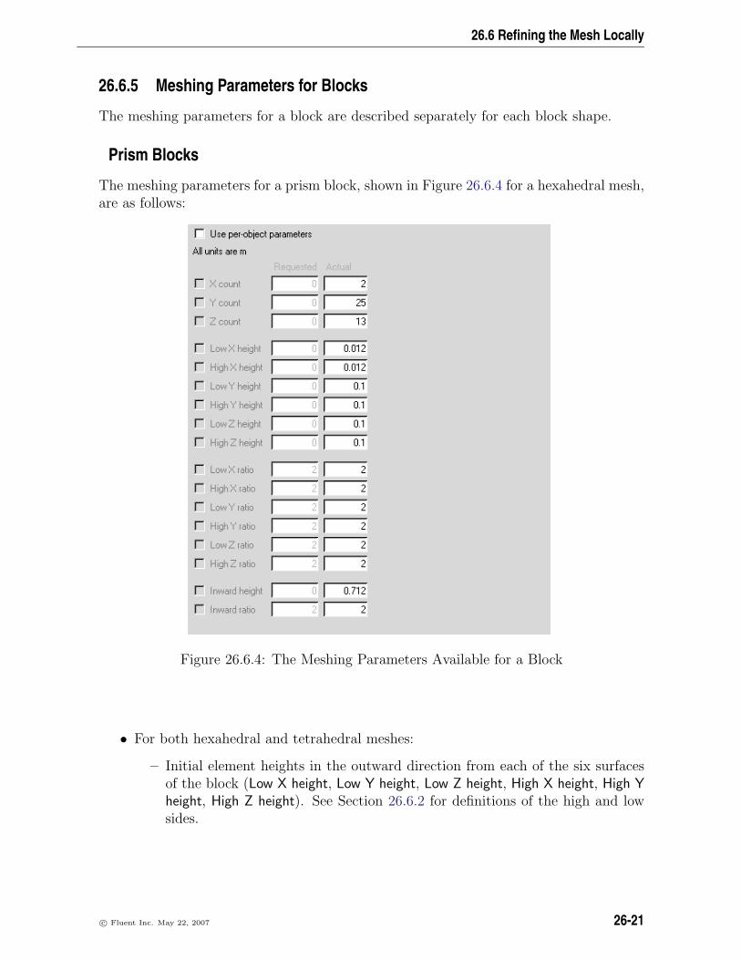
26.6 Refining the Mesh Locally
26.6.5 Meshing Parameters for Blocks
The meshing parameters for a block are described separately for each block shape.
Prism Blocks
The meshing parameters for a prism block, shown in Figure 26.6.4 for a hexahedral mesh,are as follows:
Figure 26.6.4: The Meshing Parameters Available for a Block
• For both hexahedral and tetrahedral meshes:
– Initial element heights in the outward direction from each of the six surfacesof the block (Low X height, Low Y height, Low Z height, High X height, High Yheight, High Z height). See Section 26.6.2 for definitions of the high and lowsides.
c© Fluent Inc. May 22, 2007 26-21

Generating a Mesh
• For hexahedral meshes only:
– Number of elements in each direction on the block’s edges (X count, Y count,Z count).
– Element height ratios in the outward direction from each of the six surfaces ofthe block (Low X ratio, Low Y ratio, Low Z ratio, High X ratio, High Y ratio, HighZ ratio). See Section 26.6.2 for an explanation of the element height ratio.
– Initial element height in the inward direction from the surfaces of the block(Inward height).
– Initial element height ratio in the inward direction from the surfaces of theblock (Inward ratio).
Cylinder Blocks
The meshing parameters for a cylinder block are as follows:
• For both hexahedral and tetrahedral meshes:
– Initial element heights in the outward direction from the bottom circular sur-face (Low end height) and the top circular surface (High end height).
– Initial element height in the outward direction from the block’s cylindrical sidesurface (Side height).
• For hexahedral meshes only:
– Number of elements along the diameter of the circular surfaces (Diametercount) and along the side of the cylinder (Side count).
– Initial element height in the inward direction from the cylindrical side surface(Inward height).
– Element height ratios in the outward direction from the bottom circular surface(Low end ratio) and the top circular surface (High end ratio).
– Element height ratios in the outward direction from the block’s cylindricalside surface (Side ratio) and in the inward direction from the cylindrical sidesurface (Inward ratio).
3D Polygon Blocks
The meshing parameters for a 3D polygon block are as follows:
• Number of elements along each side of the block (Side 1 count, Side 2 count, etc.)and along the height of the block (Height count).
26-22 c© Fluent Inc. May 22, 2007

26.6 Refining the Mesh Locally
• Initial element heights in the outward direction from each side of the block (Side1 height, Side 2 height, etc.) and from the bottom and top surfaces of the block(Bottom height, Top height).
• Element height ratios in the outward direction from each side of the block (Side 1ratio, Side 2 ratio, etc.) and from the bottom and top surfaces of the block (Bottomratio, Top ratio).
Ellipsoid Blocks
The meshing parameters for an ellipsoid block are as follows:
• For tetrahedral meshes only:
– Initial element heights in the outward direction from the curved surface of theblock (Curved surface size).
– Initial element heights in the outward direction from the flat surfaces of theellipsoid block that appear if you deactivate one or more octants of the block(Flat (internal) surface size).
i Note that ellipsoidal blocks cannot be meshed with the hexahedral mesher.
Elliptical Cylinder Blocks
The meshing parameters for an elliptical cylinder block are as follows:
• Initial element heights in the outward direction from the bottom elliptical surface(Low end height) and the top elliptical surface (High end height).
• Initial element height in the outward direction from the block’s cylindrical sidesurface (Side height).
• Element height ratios in the outward direction from the bottom elliptical surface(Low end ratio) and the top elliptical surface (High end ratio).
• Element height ratio in the outward direction from the block’s cylindrical sidesurface (Side ratio).
i It is recommended that you use the tetrahedral mesher when your model containselliptical cylinder blocks.
c© Fluent Inc. May 22, 2007 26-23

Generating a Mesh
26.6.6 Meshing Parameters for Fans
The meshing parameters for a cylinder or 3D polygon fan are the same as for a cylinderor 3D polygon block. See Section 26.6.5 for details.
The meshing parameters for a rectangular, circular, 2D polygon, or inclined fan are thesame as for a rectangular, circular, 2D polygon, or inclined vent. See Section 26.6.7 fordetails.
26.6.7 Meshing Parameters for Vents
The meshing parameters for a vent are described separately for each vent shape.
Circular Vents
The meshing parameters for a circular vent, shown in Figure 26.6.5 for a hexahedralmesh, are as follows:
Figure 26.6.5: The Meshing Parameters Available for a Circular Vent
• For hexahedral meshes only:
– Number of elements along the diameter of the vent (Diameter count).
26-24 c© Fluent Inc. May 22, 2007

26.6 Refining the Mesh Locally
– Initial element heights in the direction normal to the vent (Low end height,High end height). See Section 26.6.2 for definitions of the high and low sides.
If the vent is on an external wall, only the appropriate high or low side facingthe interior of the room is applicable.
– Initial element heights in the inward direction (Inward height), measured fromthe outer radius.
– Element height ratios in the direction normal to the vent (Low end ratio, Highend ratio). See Section 26.6.2 for definitions of the high and low sides.
If the vent is on an external wall, only the appropriate high or low side facingthe interior of the room is applicable.
– Element height ratios in the inward direction (Inward ratio), measured fromthe outer radius.
• For tetrahedral meshes only:
– Initial element height of the first element next to the vent (Element height).
Rectangular Vents
The meshing parameters for a rectangular vent are as follows:
• For hexahedral meshes only:
– Number of elements along the edges of the vent (X count, Y count; Y count, Zcount; or X count, Z count; depending on the plane in which the vent lies).
– Initial element heights in the direction normal to the vent (Low end height,High end height). See Section 26.6.2 for definitions of the high and low sides.
If the vent is on an external wall, only the appropriate high or low side facingthe interior of the room is applicable.
– Initial element height in the inward direction (Inward height) for both coordi-nate directions on the surface of the vent.
– Element height ratios in the direction normal to the vent (Low end ratio, Highend ratio). See Section 26.6.2 for definitions of the high and low sides.
If the vent is on an external wall, only the appropriate high or low side facingthe interior of the room is applicable.
– Element height ratios in the inward direction (Inward ratio) for both coordinatedirections on the surface of the vent.
i Only two of the three parameters (number of elements, inward height, and in-ward ratio) can be specified for any coordinate direction. The third parameteris determined from the other two.
c© Fluent Inc. May 22, 2007 26-25

Generating a Mesh
• For tetrahedral meshes only:
– Initial element height of the first element next to the vent (Tetra size).
Inclined Vents
The meshing parameters for an inclined vent are as follows:
• For hexahedral meshes only:
– Number of elements in the coordinate direction along which the vent is inclined(X count, Y count, or Z count), and in the other two directions (Y-Z count,X-Z count, or X-Y count).
– Initial element heights in the direction normal to the vent (Low end height,High end height). See Section 26.6.2 for definitions of the high and low sides.
– Element height ratios in the direction normal to the vent (Low end ratio, Highend ratio). See Section 26.6.2 for definitions of the high and low sides.
• For tetrahedral meshes only:
– Initial element height of the first element next to the vent (Tetra size).
2D Polygon Vents
The meshing parameters for a 2D polygon vent are as follows:
• For both hexahedral and tetrahedral meshes:
– Number of elements along each side of the vent (Side 1 count, Side 2 count,etc.).
– Initial element heights in the outward direction from the bottom and topsurfaces of the vent (Bottom height, Top height).
– Element height ratios in the outward direction from the bottom and top sur-faces of the vent (Bottom ratio, Top ratio).
26.6.8 Meshing Parameters for Openings
The meshing parameters for a rectangular, circular, 2D polygon, or inclined opening arethe same as for a rectangular, circular, 2D polygon, or inclined vent. See Section 26.6.7for details.
26-26 c© Fluent Inc. May 22, 2007

26.6 Refining the Mesh Locally
26.6.9 Meshing Parameters for Person Objects
The meshing parameters for the head, body, arms, legs, or thighs of a person are thesame as for a prism block. See Section 26.6.5 for details.
The meshing parameters for the face of a person are the same as for a rectangular vent.See Section 26.6.7 for details.
26.6.10 Meshing Parameters for Walls
The meshing parameters for a wall are described separately for each wall shape.
Rectangular Walls
The meshing parameters for a rectangular wall, shown in Figure 26.6.6 for a hexahedralmesh, are as follows:
Figure 26.6.6: The Meshing Parameters Available for a Wall
• For hexahedral meshes only:
– Number of elements along the edges of the wall (X count, Y count; Y count, Zcount; or X count, Z count; depending on the plane in which the wall lies).
– Initial element height in the direction normal to the wall (Element height).
– Initial element height in the inward direction (Inward height) for both coordi-nate directions on the surface of the wall.
c© Fluent Inc. May 22, 2007 26-27

Generating a Mesh
– Element height ratio in the direction normal to the wall (Element ratio).
– Element height ratio in the inward direction (Inward ratio) for both coordinatedirections on the surface of the wall.
i Only two of the three parameters (number of elements, inward height, and in-ward ratio) can be specified for any coordinate direction. The third parameteris determined from the other two.
• For tetrahedral meshes only:
– Initial element height of the first element next to the wall (Tetra size).
Circular, 2D Polygon, and Inclined Walls
The meshing parameters for a circular, 2D polygon, or inclined wall are the same as fora circular, 2D polygon, or inclined vent, except no distinction is made between low andhigh end (side) for a wall. See Section 26.6.7 for details.
26.6.11 Meshing Parameters for Partitions
The meshing parameters for a rectangular, circular, 2D polygon, or inclined partition arethe same as for a rectangular, circular, 2D polygon, or inclined vent. See Section 26.6.7for details.
Note that you can specify the number of elements in the direction of the partition thick-ness using Inward height, or Thickness count for an inclined partition. If the partition hasa zero thickness, this parameter is not applicable.
26.6.12 Meshing Parameters for Sources
The meshing parameters for a prism, cylinder, ellipsoid, or elliptical cylinder source arethe same as for a prism, cylinder, ellipsoid, or elliptical cylinder block. See Section 26.6.5for details.
The meshing parameters for a rectangular, circular, 2D polygon, or inclined source arethe same as for a rectangular, circular, 2D polygon, or inclined vent. See Section 26.6.7for details.
26.6.13 Meshing Parameters for Resistances
The meshing parameters for a prism, cylinder, or polygon resistance are the same as fora prism, cylinder, or polygon block. See Section 26.6.5 for details.
26-28 c© Fluent Inc. May 22, 2007

26.6 Refining the Mesh Locally
26.6.14 Meshing Parameters for Heat Exchangers
The meshing parameters for a rectangular, circular, inclined, or 2D polygon heat ex-changer are the same as for a rectangular, circular, inclined, or 2D polygon vent. SeeSection 26.6.7 for details.
26.6.15 Meshing Parameters for Hoods
The meshing parameters for the neck of a hood are the same as for a prism block. SeeSection 26.6.5 for details.
The meshing parameters for the canopy of a hood are the same as for a 3D polygonblock. See Section 26.6.5 for details.
The meshing parameters for the individual parts of the flange or the exhausts in the hoodare the same as for a rectangular vent. See Section 26.6.7 for details.
26.6.16 Meshing Parameters for Assemblies
The meshing parameters for the bounding box of an assembly are essentially a combina-tion of the per-object parameters for a hollow block and a room, and are available onlyfor hexahedral meshes.
The external meshing parameters for an assembly begin with Outside and are the sameas those for a hollow block (see Section 26.6.5), with the exception that the inward heightand inward ratio are not applicable. The internal meshing parameters begin with Inside,and are the same as those for a room (see Section 26.6.4), with the addition of Inside Xmax size, Inside Y max size, and Inside Z max size. These three parameters are similar tothe global maximum size parameters (i.e., Max X size, Max Y size, Max Z size) for theentire Airpak model (see Section 26.5.1), except that they apply to the interior of theassembly bounding box.
c© Fluent Inc. May 22, 2007 26-29

Generating a Mesh
26.7 Controlling the Meshing Order for Objects
By default, objects are meshed in the order in which they were created. If two or moreobjects intersect, meshing the objects in the creation order may not give the result thatyou want. For such cases, you can modify the meshing order by changing the objectpriorities for the intersecting objects. The object with a higher priority (higher number)will retain the mesh where it intersects with an object with a lower priority.
To modify the meshing priorities, select Edit priorities in the Model menu.
Model−→Edit priorities
This will open the Object priority panel (Figure 26.7.1), which allows you to changethe meshing order of the objects that have been created. Simply edit the priorities asrequired, and then click Accept to save the new meshing order. You can also change thepriorities by dragging an object up or dwn in the Model manager window.
Figure 26.7.1: The Object priority Panel
26-30 c© Fluent Inc. May 22, 2007

26.8 Non-Conformal Meshing Procedures for Assemblies
26.8 Non-Conformal Meshing Procedures for Assemblies
In Airpak, assemblies of objects can be meshed separately. A region can be defined arounda particular assembly and this region can be meshed independently of the mesh outsideit. At the interface with the main model, there is a many-to-one transition between themesh cells inside the region and those outside it, and a non-conformal interface is createdat the boundary between the meshes. This allows for the embedding of a fine mesh withinthe sub-region around an assembly where it is needed, and for a coarse mesh in the restof the model. To use non-conformal meshing for assemblies, you will use the followingprocedure:
1. Right-click on the assembly in the Model manager, and select Edit object from thecontext menu.
2. In the Meshing tab of the Assemblies panel, turn on the Mesh separately option.
3. If required, add a “slack” region around the assembly.
(a) Under Slack, enter the desired offset distances in the Min X, Y, Z and Max X,Y, Z directions. Positive values prescribe a slack region toward the exterior ofthe assembly.
By default the bounding box of the assembly has the exact extent necessary toenclose the objects that make the assembly. Defining a slack region allows you tomake the bounding box slightly larger. This will make it possible to mesh moreassemblies separately. Where a foreign object crosses the bounding box of an assem-bly, the non-conformal interface will cross through that object. See Section 7.8.2for more details on specifying the slack distance around the bounding box of theassembly.
i The bounding box must be large enough so that the cells on both sides ofthe box are either both fluid or both solid, with the same material.
Multiple assemblies can be meshed separately provided that:
• Assemblies are not partially embedded within one another (i.e., the boundingbox of one assembly cannot intersect the bounding box of another assembly).
4. If required, specify the Minimum gap that separates objects in the assembly. SeeSection 7.8.2 for more details on specifying the Minimum gap.
5. If required, specify the Mesh type to mesh the objects in the assembly. See Sec-tion 7.8.2 for more details on specifying the Mesh type.
6. In the Mesh control panel, turn on the Mesh assemblies separately option.
Note that both the hexa-unstructured and hexa-cartesian meshers can be used tomesh assemblies separately, using non-conformal meshing. See Section 26.3.1 for
c© Fluent Inc. May 22, 2007 26-31

Generating a Mesh
more information on hexahedral meshing in Airpak. The tetra mesher does notcurrently allow non-conformal meshing.
7. If required, turn on the Allow different subgrid types option in the Mesh control panel.This allows you to generate a mesh type for the assemblies different from the globalmesh type, as specified under Mesh type in the Meshing tab of the Assemblies panel.
i When the meshing procedure has been completed, any assembly that has beenmeshed separately from the rest of the model will have its name displayed in adifferent color (default is pink) in the Model manager window.
26.9 Displaying the Mesh
Once you have generated a mesh, you can examine it to determine if it meets yourneeds. Airpak provides tools for viewing the mesh on individual objects, as well as oncross-sectional planes that extend throughout the room.
26.9.1 Displaying the Mesh on Individual Objects
The procedure for displaying the mesh on the surfaces or edges of objects or insidevolumetric objects is as follows:
1. Open the Mesh control panel by selecting Generate mesh in the Model menu, or by
clicking on the button in the Model and solve toolbar.
Model−→Generate mesh
2. Click on the Display tab to show the mesh display tools (see Figure 26.9.1).
3. Select one or more of the following display options:
• Choose Surface to display the mesh on the exterior faces of objects. An ex-ample is shown in Figure 26.9.2.
• Choose Volume to display the mesh inside volumetric objects (e.g., cylinderblocks, prism resistances). An example is shown in Figure 26.9.3.
i Note that the Wire option is selected by default. If the Wire option isnot selected, the mesh lines will not be displayed.
26-32 c© Fluent Inc. May 22, 2007

26.9 Displaying the Mesh
Figure 26.9.1: The Display Tab of the Mesh control Panel
4. Specify the objects for which you want to display the mesh:
• Choose All objects to display the mesh on all objects in the model.
• Choose Current type to display the mesh only on objects of the type currentlyselected in the Model manager window. For example, if a block object isselected, the mesh will be displayed only on block objects.
• Choose Selected objects to display the mesh only on the objects that are cur-rently selected in the Model manager window. You can select the object eitherin the graphics window or in the Model manager window.
• Choose Selected shape to display the mesh only on objects of the shape cur-rently selected in the Model manager window. For example, if a rectangular
c© Fluent Inc. May 22, 2007 26-33

Generating a Mesh
Figure 26.9.2: Display of Surface Elements
Figure 26.9.3: Display of Volume Elements
26-34 c© Fluent Inc. May 22, 2007

26.9 Displaying the Mesh
partition is selected, the mesh will be displayed only on 2D rectangular objects(e.g., rectangular vent, rectangular fan, etc.).
5. If you want to add filled shading to the mesh display, rather than displaying justthe mesh lines, turn on the Solid option. When this option is off, the mesh willappear as shown in Figure 26.9.2. When it is on, the mesh will appear as shownin Figure 26.9.4. The mesh lines will not be displayed when the Wire option is off.When the Solid option is on and the Wire option is off, the mesh will appear as asolid without the mesh lines.
Figure 26.9.4: Filled Solid Display
6. Under Non-conformal, turn on Inner or Outer, or both, if you want Airpak to displaythe mesh on the inner side and/or the outer side of the non-conformal interface forassemblies that were meshed separately.
7. To display the common mesh faces between assemblies touching other assemblies,turn on Between assemblies.
c© Fluent Inc. May 22, 2007 26-35

Generating a Mesh
8. Turn on the Display mesh option.
You can change the color of the mesh on objects using the Graphical styles panel. SeeSection 6.3.6 for details.
26.9.2 Displaying the Mesh on a Cross-Section of the Model
In addition to displaying the mesh on individual objects, as described in Section 26.9.1,you can also display the mesh on the intersection of a plane with the model (i.e., on across-section of the model). Anexample is shown in Figure 26.9.5.
Figure 26.9.5: Mesh Display on a Cross-Sectional Plane
The procedure for displaying the mesh on a cross-sectional plane is as follows:
1. Open the Mesh control panel by selecting Generate mesh in the Model menu, or by
clicking on the button in the Model and solve toolbar.
Model−→Generate mesh
2. Click on the Display tab to show the mesh display tools (see Figure 26.9.1).
3. Turn on the Cut plane option.
4. Define the plane on which to display the mesh, using one of the following fourmethods:
26-36 c© Fluent Inc. May 22, 2007

26.9 Displaying the Mesh
• Specify a plane cut through the center of the model that is aligned with anyCartesian axis by selecting X plane through center, Y plane through center, orZ plane through center in the Set position drop-down list.
• Specify a point on the plane and the normal direction to the plane:
(a) Select Point and normal in the Set position drop-down list.
(b) Enter the coordinates of a point on the plane (PX, PY, PZ).
i If the Display mesh option is already turned on, you must press the<Enter> key on your keyboard after entering each value.
(c) Enter a vector defining the direction normal to the plane (NX, NY, NZ).For example, entering (1, 0, 0) for the vector will define a normal pointingin the x direction.
i If the Display mesh option is already turned on, you must press the<Enter> key on your keyboard after entering each value.
• Specify an equation that defines the plane:
(a) Select the Coeffs (Ax + By + Cz = D) option.
(b) Enter the coefficients A, B, C, and D for the equation
Ax+By + Cz = D (26.9-1)
i If the Display mesh option is already turned on, you must press the<Enter> key on your keyboard after entering each value.
• Specify the plane using your mouse:
(a) Use the Orient menu to specify the desired orientation. If you require ahorizontal or vertical plane through your model, choose the orientationsuch that the plane of the display screen is perpendicular to the desiredmesh-display plane. For example, if you want to display the mesh on ay-z or x-y plane, choose Orient positive Y as the orientation so that thedisplay-screen plane is the x-z plane (see Figure 26.9.6). If you want tospecify the plane by selecting three points on it, orient your model asdesired.
(b) Select Horizontal - screen select, Vertical - screen select, or 3 points - screenselect in the Set position drop-down list.
(c) If you selected Horizontal - screen select or Vertical - screen select, clickyour left mouse button in the graphics window to indicate a point on thedesired plane. Airpak will display the mesh on a horizontal or vertical planeperpendicular to the plane of the graphics screen and passing through the
c© Fluent Inc. May 22, 2007 26-37

Generating a Mesh
Figure 26.9.6: Specification of a Vertical Cross-Section
selected point. In Figure 26.9.6, the vertical mesh plane is indicated by avertical line passing through the model. Figure 26.9.7 shows an isometricview of the same mesh plane.
If you selected 3 points - screen select, select the first, second, and thirdpoints on the plane in the graphics window using the left mouse button.Each point must be on the edge of an object or the room. If it is not,Airpak will move the point to the nearest location on the edge of an objector the room. Airpak will display the mesh on the plane defined by the threepoints.
i Note that if you display a hexahedral mesh on a plane that is notparallel or perpendicular to the sides of the room, the mesh elementsmay look like the elements of a tetrahedral mesh. This is an opticalillusion caused by Airpak when it displays a hexahedral mesh on aplane that is not horizontal or vertical relative to the sides of theroom.
5. Turn on the Display mesh option.
6. If you want to change the color of the mesh display, click on the colored squarenext to Mesh color, and select a new color. Acceptable entries include white (thedefault), red, blue, green, orange, yellow, etc.
7. To advance the currently-displayed mesh plane through the room so that you caneasily view the mesh on different cross-sectional planes, use the slider bar next to
26-38 c© Fluent Inc. May 22, 2007
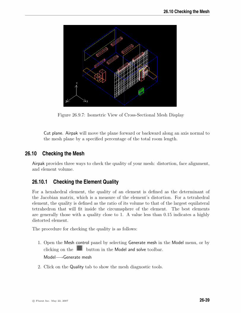
26.10 Checking the Mesh
Figure 26.9.7: Isometric View of Cross-Sectional Mesh Display
Cut plane. Airpak will move the plane forward or backward along an axis normal tothe mesh plane by a specified percentage of the total room length.
26.10 Checking the Mesh
Airpak provides three ways to check the quality of your mesh: distortion, face alignment,and element volume.
26.10.1 Checking the Element Quality
For a hexahedral element, the quality of an element is defined as the determinant ofthe Jacobian matrix, which is a measure of the element’s distortion. For a tetrahedralelement, the quality is defined as the ratio of its volume to that of the largest equilateraltetrahedron that will fit inside the circumsphere of the element. The best elementsare generally those with a quality close to 1. A value less than 0.15 indicates a highlydistorted element.
The procedure for checking the quality is as follows:
1. Open the Mesh control panel by selecting Generate mesh in the Model menu, or by
clicking on the button in the Model and solve toolbar.
Model−→Generate mesh
2. Click on the Quality tab to show the mesh diagnostic tools.
c© Fluent Inc. May 22, 2007 26-39

Generating a Mesh
3. Select the Quality option. Airpak will show a histogram of the element quality, asshown in Figure 26.10.1.
Figure 26.10.1: The Quality Histogram in the Mesh control Panel
4. If you want to modify the range of quality values viewed, enter a new value inthe Min or Max field and then press the <Enter> key on your keyboard or clickReplot to update the histogram. To modify the maximum height of the bars or thenumber of bars in the histogram, enter a new value in the Height and/or Bars fieldsand click Replot. (Note that a Height of 0 instructs Airpak to display the bars ofthe histogram at their full height.) To return to the default ranges, click the Resetbutton.
5. To view the elements of the mesh within a particular range of quality values, clickon a bar in the histogram. Airpak will display the elements in the selected rangein the graphics window. Select the Solid option if you want to view these elementswith solid shading.
26-40 c© Fluent Inc. May 22, 2007

26.10 Checking the Mesh
26.10.2 Checking the Face Alignment
Face alignment is a measure of mesh quality defined by
face alignment index = ~c0c1 · ~f (26.10-1)
where c0 and c1 are the centroids of two adjacent elements, and ~f is the normal vectorto the face between the two elements, as shown in the 2D example in Figure 26.10.2.
Figure 26.10.2: Definition of Face Alignment
Adjacent mesh faces that are not aligned can result in long, narrow elements. A value of1 indicates perfect alignment. Values less than 0.15 indicate a severely distorted mesh.
The procedure for checking the face alignment is as follows:
1. Open the Mesh control panel by selecting Generate mesh in the Model menu, or by
clicking on the button in the Model and solve toolbar.
Model−→Generate mesh
2. Click on the Quality tab to show the mesh diagnostic tools.
3. Select the Face alignment option. Airpak will show a histogram of the face alignment,as shown in Figure 26.10.3.
4. If you want to modify the range of face alignments viewed, enter a new value inthe Min or Max field and then press the <Enter> key on your keyboard or clickReplot to update the histogram. To modify the maximum height of the bars or thenumber of bars in the histogram, enter a new value in the Height and/or Bars fieldsand click Replot. (Note that a Height of 0 instructs Airpak to display the bars ofthe histogram at their full height.) To return to the default ranges, click the Resetbutton.
5. To view the elements of the mesh within a particular range of face alignments, clickon a bar in the histogram. Airpak will display the elements in the selected rangein the graphics window. Select the Solid option if you want to view these elementswith solid shading.
c© Fluent Inc. May 22, 2007 26-41

Generating a Mesh
Figure 26.10.3: The Face alignment Histogram in the Mesh control Panel
26.10.3 Checking the Element Volume
Extremely small elements (on the order of 10−12 or lower) can lead to problems in thesolver. It is therefore important to check the minimum element volumes in your mesh.Although this situation should and can be avoided in most models, if your model musthave very small elements, you may want to use the double precision version of the solver(see Section 27.6).
The procedure for checking the element volume is as follows:
1. Open the Mesh control panel by selecting Generate mesh in the Model menu, or by
clicking on the button in the Model and solve toolbar.
Model−→Generate mesh
2. Click on the Quality tab to show the mesh diagnostic tools.
26-42 c© Fluent Inc. May 22, 2007

26.10 Checking the Mesh
3. Select the Volume option. Airpak will show a histogram of the element volume, asshown in Figure 26.10.4.
Figure 26.10.4: The Volume Histogram in the Mesh control Panel
4. If you want to modify the range of volumes viewed, enter a new value in the Minor Max field and then press the <Enter> key on your keyboard or click Replot toupdate the histogram. To modify the maximum height of the bars or the numberof bars in the histogram, enter a new value in the Height and/or Bars fields andclick Replot. (Note that a Height of 0 instructs Airpak to display the bars of thehistogram at their full height.) To return to the default ranges, click the Resetbutton.
5. To view the elements of the mesh within a particular range of volumes, click on abar in the histogram. Airpak will display the elements in the selected range in thegraphics window. Select the Solid option if you want to view these elements withsolid shading.
c© Fluent Inc. May 22, 2007 26-43

Generating a Mesh
26.11 Exporting a Mesh
Airpak allows you to export mesh data to I-DEAS or ANSYS. The general procedure forexporting a mesh file from Airpak is as follows:
1. Open the Mesh control panel by selecting Generate mesh in the Model menu, or by
clicking on the button in the Model and solve toolbar.
Model−→Generate mesh
2. Click on the Export tab to show the export options, as shown in Figure 26.11.1.
Figure 26.11.1: The Export Tab in the Mesh control Panel
3. Click the appropriate button for exporting either an I-DEAS or an ANSYS file andfollow the procedure in Section 26.11.1 or 26.11.2.
26-44 c© Fluent Inc. May 22, 2007

26.12 Loading an Existing Mesh
26.11.1 Exporting an I-DEAS Neutral File
To export an I-DEAS neutral file from Airpak, use the following procedure:
1. In the Export tab of the Mesh control panel, click Export as IDEAS neutral file. Thiswill open the I-DEAS neutral file panel (Figure 26.11.2).
Figure 26.11.2: The I-DEAS neutral file Panel
2. In the I-DEAS neutral file panel, enter a name for the file to be saved (with a .ideas
extension) next to File name and click Save. The Message window will report whenthe file has been written.
26.11.2 Exporting an ANSYS Grid File
To export an ANSYS grid file from Airpak, use the following procedure:
1. In the Export tab of the Mesh control panel, click Export as Ansys grid file. This willopen the ANSYS file panel (Figure 26.11.3).
2. In the ANSYS file panel, enter a name for the file to be saved (with a .ansys
extension) next to File name and click Save. The Message window will report whenthe file has been written.
26.12 Loading an Existing Mesh
When you read an existing job into Airpak, the mesh is not automatically loaded. If youhave already created a mesh for the model, you can load it into Airpak by clicking theLoad mesh button in the Mesh control panel (Figure 26.4.1 or 26.4.2).
c© Fluent Inc. May 22, 2007 26-45

Generating a Mesh
Figure 26.11.3: The ANSYS file Panel
26-46 c© Fluent Inc. May 22, 2007

Chapter 27. Calculating a Solution
Once you have built your model (see Chapters 8–19) and generated a mesh (see Chap-ter 26), you are ready to calculate a solution. Airpak allows you to specify the parametersthat control the solution procedure and to monitor the solution. The functions that areneeded to define the solution procedure are found in the Model manager window, underthe Problem setup and Solution settings nodes, and in the Solve menu. This chapter be-gins with an overview of the Solve menu and the solution settings in the Model managerwindow, and then describes how to define the solution procedure for your model. Onceyou have calculated a solution for your simulation, you will go on to examine the resultsof the simulation, as described in Chapters 28 and 29.
The information in this chapter is divided into the following sections:
• Section 27.1: Overview
• Section 27.2: General Procedure for Setting Up and Calculating a Solution
• Section 27.3: Choosing the Discretization Scheme
• Section 27.4: Setting Under-Relaxation Factors
• Section 27.5: Selecting the Multigrid Scheme
• Section 27.6: Selecting the Version of the Solver
• Section 27.7: Initializing the Solution
• Section 27.8: Monitoring the Solution
• Section 27.9: Defining Postprocessing Objects
• Section 27.10: Defining Reports
• Section 27.11: Setting the Solver Controls
• Section 27.12: Performing Calculations
• Section 27.13: Diagnostic Tools for Technical Support
c© Fluent Inc. May 22, 2007 27-1

Calculating a Solution
27.1 Overview
The Solve menu (Figure 27.1.1) is used in conjunction with the Problem setup and Solutionsettings nodes of the Model manager window to define the solution parameters for yourAirpak model.
Figure 27.1.1: The Solve Menu
The functions you need to define the solution parameters for your Airpak simulationinclude the following:
• specifying the parameters that control the solver
Problem setup−→ Basic parameters
• changing the variables to be monitored during the solution calculation
Solve−→Solution monitor
• defining the solution procedure
Solution settings−→ Basic settings or Solve−→Settings−→Basic
Solution settings−→ Advanced settings or Solve−→Settings−→Advanced
• accessing or creating files for use by your technical support engineer
Solve−→Diagnostics
• defining the format for reports
Solve−→Define report
In addition to solution control functions, the Solve menu contains a function related tomanaging multiple solution trials (Solve−→Define trials). This function is described inChapter 24.
27-2 c© Fluent Inc. May 22, 2007

27.2 General Procedure for Setting Up and Calculating a Solution
27.2 General Procedure for Setting Up and Calculating a Solution
Once you have built your model in Airpak, you are ready to calculate a solution. Thefollowing steps outline a general procedure you can follow:
1. Choose the discretization scheme (see Section 27.3).
2. Set the under-relaxation factors (see Section 27.4).
3. Select the multigrid scheme (see Section 27.5).
4. Select the version of the solver (single precision or double precision) (see Sec-tion 27.6).
5. Initialize the solution (see Section 27.7).
6. Enable the appropriate solution monitors (see Section 27.8).
7. Define postprocessing objects prior to solving the model (see Section 27.9).
8. Define the reports that you want Airpak to create when the solution is complete(see Section 27.10).
9. Specify the parameters that control the solver (see Section 27.11).
10. Start calculating (see Section 27.12).
The default settings for the first three items listed above are suitable for most problemsand need not be changed. The following sections outline how these and other solutionparameters can be changed, and when you may wish to change them. The steps listedabove apply for all steady-state calculations. See Chapter 20 for information aboutunsteady solution procedures.
c© Fluent Inc. May 22, 2007 27-3

Calculating a Solution
27.3 Choosing the Discretization Scheme
Airpak allows you to choose the discretization scheme for the convection terms of eachgoverning equation. See Section 31.6.2 for a complete description of the discretizationschemes available in Airpak.
You can choose the discretization scheme to be used in the Advanced solver setup panel(Figure 27.3.1).
Solution settings−→ Advanced settings (or Solve−→Settings−→Advanced)
Figure 27.3.1: The Advanced solver setup Panel
The discretization scheme to be used for each of the equations that Airpak solves is
27-4 c© Fluent Inc. May 22, 2007

27.4 Setting Under-Relaxation Factors
specified under Discretization scheme in the Advanced solver setup panel. By default,all equations (except the pressure equation) are solved using a first-order scheme. Thisscheme gives you a relatively quick and accurate solution. The second-order scheme isavailable for cases in which you require a more accurate solution. Be aware, however, thata second-order solution may take longer to converge. Also, for a second-order calculationit is recommended that you first compute a first-order solution and use it as a startingpoint.
By default, the pressure equation is solved using the Standard scheme. The Body ForceWeighted scheme is also available, but it is recommended that you keep the defaultstandard scheme for most cases. A second-order scheme is also available for cases inwhich you require a more accurate solution.
27.4 Setting Under-Relaxation Factors
As discussed in Section 31.6.2, Airpak uses under-relaxation to control the update ofcomputed variables at each iteration. This means that all equations solved using Airpakwill have under-relaxation factors associated with them.
You can set the under-relaxation factors in the Advanced solver setup panel (Figure 27.3.1).
Solution settings−→ Advanced settings (or Solve−→Settings−→Advanced)
The value of the “under-relaxation factor” for each of the equations that Airpak solvesis specified under Under-relaxation in the Advanced solver setup panel. Because of thenonlinearity of the equation set, it is necessary to reduce the change of a variable fromone iteration to the next. This is referred to as under-relaxation. For example, if thepressure under-relaxation factor is 0.3, the change in pressure value from one iterationto the next will be restricted to 30% of the difference between the initial value and thenewly calculated value.
In Airpak, the default under-relaxation parameters for all variables are set to values thatare near optimal for the largest possible number of cases. These values are suitable formany problems, but for some particularly non-linear problems (e.g., some turbulent flowsor high-Rayleigh-number natural-convection problems) it is prudent to reduce the under-relaxation factors initially. If you click Reset in the Basic settings panel (Figure 27.7.1),Airpak adjusts the under-relaxation factors to values that are recommended for the typeof problem you are trying to solve.
It is good practice to begin a calculation using the default settings in the Advanced solversetup panel. For most flows, the default under-relaxation factors do not usually requiremodification. If the solution exhibits unstable or divergent behavior, you may need tomodify the under-relaxation factors; however, inappropriate under-relaxation factors maydecrease the rate of convergence for your problem. Please contact your technical supportengineer if your solution displays divergent behavior.
c© Fluent Inc. May 22, 2007 27-5

Calculating a Solution
27.5 Selecting the Multigrid Scheme
As discussed in Section 31.6.4, Airpak uses a multigrid scheme to accelerate solutionconvergence. You can set the parameters related to the multigrid solver in the Advancedsolver setup panel (Figure 27.3.1).
Solution settings−→ Advanced settings (or Solve−→Settings−→Advanced)
You can specify parameters related to the multigrid solver under Linear solver in theAdvanced solver setup panel. The multigrid solver accelerates solution convergence byusing a sequence of coarse grids based on the computational grid created by Airpak.Solutions can be computed more quickly on a coarse grid, but coarse-grid solutions arenot as accurate as fine-grid solutions. For this reason, Airpak uses the coarser grid levelsto obtain a starting point for the final solution, which is obtained for the actual Airpakgrid. The following options are available for the multigrid solver.
Type specifies the multigrid cycle type for each equation that Airpak solves. (SeeSection 31.6.4 for a description of the different multigrid cycles.) By default, theV cycle is used for the pressure equation and the flex cycle is used for all otherequations. You should generally not need to modify these settings.
Termination criterion controls the multigrid solver in different ways for different cycles.For the flex cycle, the Termination criterion governs when the solver should return toa finer grid level (i.e., when the residuals have improved sufficiently on the currentlevel). For the V and W cycles, the Termination criterion determines whether or notanother cycle should be performed on the finest (original) grid level. If the currentresidual on the finest level does not satisfy the Termination criterion, Airpak willperform another multigrid cycle.
For most cases, you should not need to modify the settings for the Terminationcriterion.
Residual reduction tolerance dictates when a coarser grid level must be visited (due toinsufficient improvement in the solution on the current level). This parameter isused only by the flex cycle. With a larger value of the Residual reduction tolerance,coarse levels will be visited less often (and vice versa).
For most cases, you should not need to modify the settings for the Residual reductiontolerance.
27-6 c© Fluent Inc. May 22, 2007

27.6 Selecting the Version of the Solver
27.6 Selecting the Version of the Solver
In the Advanced solver setup panel (Figure 27.3.1), select the version of the solver youwant to use in the Precision drop-down list.
Single specifies that the single-precision version of the solver is to be used.
Double specifies that the double-precision version of the solver is to be used.
Both single-precision and double-precision versions of Airpak are available on all computerplatforms. For most cases, the single-precision solver will be sufficiently accurate, butcertain types of problems may benefit from the use of a double-precision solver. Severalexamples are listed below:
• For conjugate problems with high thermal-conductivity ratios and/or high-aspect-ratio grids, convergence and/or accuracy may be impaired with the single-precisionsolver, due to inefficient transfer of boundary information.
• If your geometry has features of very disparate length scales (e.g., a quasi 2Dmodel), single-precision calculations may not be adequate to represent the nodecoordinates.
27.7 Initializing the Solution
Before starting your CFD simulation, you must supply Airpak with the number of itera-tions to be performed and the criteria Airpak should use to check for convergence. Youcan specify the number of iterations and the convergence criteria in the Basic settingspanel (Figure 27.7.1).
Solution settings−→ Basic settings (or Solve−→Settings−→Basic)
The following values should be specified in the Solver setup panel.
1. Specify the Number of iterations to be performed by Airpak during the calculation.This specifies the number of solution iterations to be performed in a steady-statecalculation. The calculation will stop when these iterations have been performed orthe Convergence criteria are satisfied, whichever happens first. For relatively simplemodels, the default of 100 should be sufficient for the solution to converge, butfor more complex models you may need to increase this value. See Chapter 20 fordetails on specifying the number of iterations for a transient simulation.
2. Specify the Convergence criteria. These are the solution-residual values used todetermine convergence. Solution residuals measure the error or imbalance in theconservation equations that Airpak solves, and are defined in Section 31.6.5. When
c© Fluent Inc. May 22, 2007 27-7

Calculating a Solution
Figure 27.7.1: The Basic settings Panel
all solution residuals (e.g., flow, energy, turbulence, species) are less than or equalto their specified convergence criteria, the solution will be considered converged.If you click Reset in the Basic settings panel, Airpak will adjust the convergencecriteria to values that are suitable for the type of problem you are trying to solve.
i Note that when you click on Reset in the Basic settings panel, Airpak computesapproximate values of the Reynolds, Peclet, Rayleigh, and Prandtl numbers, basedon the physical characteristics of the model you have defined, and displays themin the Message window. See Section 6.4.4 for more details on the Reynolds, Peclet,Rayleigh, and Prandtl numbers.
27.8 Monitoring the Solution
The equations of flow and heat transfer are highly non-linear. To solve these equationsnumerically, an iterative procedure is required. Monitoring the convergence visuallyallows you to observe the ongoing results of the iterative procedure for each of the primaryvariables, and to determine the rate of convergence and how close the solution is tocompletion. See Section 31.6.5 for more details on solution convergence.
27.8.1 Defining Solution Monitors
The Solution monitor parameters panel (Figure 27.8.1) allows you to specify the variablesto be monitored during the calculation. To open the Solution monitor parameters panel,
select Run solution in the Solve menu or click on the button in the Model and solvetoolbar.
27-8 c© Fluent Inc. May 22, 2007

27.8 Monitoring the Solution
Solve−→Run solution
This opens the Solve panel. Next, select the Start monitor option and click on the Editparameters button. This will open the Solution monitor parameters panel.
Figure 27.8.1: The Solution monitor definition Panel
To define the solution monitors for your simulation, follow the steps below.
1. Specify a Solution ID for the solver calculation for which you wish to view thesolution residuals and point monitors. This defines a unique identifier for thesolution results. Airpak automatically creates a default name that you can alter bytyping a new name in the Solution ID text entry field. The default name consists ofthe project name plus a two-digit sequential number, starting with 00. When youclick Create the solution residuals and point monitors for the selected calculationwill be displayed in separate Solution residuals and Monitor graphics display andcontrol windows.
2. Specify the Variable for which the convergence is to be displayed. The followingoptions are available:
All enables the display of residuals for pressure, temperature, and the x, y, andz velocity components.
None disables the display of all residuals.
c© Fluent Inc. May 22, 2007 27-9
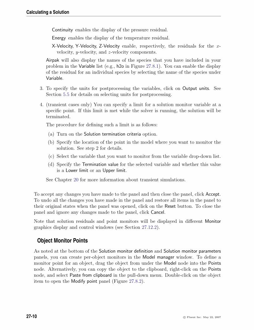
Calculating a Solution
Continuity enables the display of the pressure residual.
Energy enables the display of the temperature residual.
X-Velocity, Y-Velocity, Z-Velocity enable, respectively, the residuals for the x-velocity, y-velocity, and z-velocity components.
Airpak will also display the names of the species that you have included in yourproblem in the Variable list (e.g., h2o in Figure 27.8.1). You can enable the displayof the residual for an individual species by selecting the name of the species underVariable.
3. To specify the units for postprocessing the variables, click on Output units. SeeSection 5.5 for details on selecting units for postprocessing.
4. (transient cases only) You can specify a limit for a solution monitor variable at aspecific point. If this limit is met while the solver is running, the solution will beterminated.
The procedure for defining such a limit is as follows:
(a) Turn on the Solution termination criteria option.
(b) Specify the location of the point in the model where you want to monitor thesolution. See step 2 for details.
(c) Select the variable that you want to monitor from the variable drop-down list.
(d) Specify the Termination value for the selected variable and whether this valueis a Lower limit or an Upper limit.
See Chapter 20 for more information about transient simulations.
To accept any changes you have made to the panel and then close the panel, click Accept.To undo all the changes you have made in the panel and restore all items in the panel totheir original states when the panel was opened, click on the Reset button. To close thepanel and ignore any changes made to the panel, click Cancel.
Note that solution residuals and point monitors will be displayed in different Monitorgraphics display and control windows (see Section 27.12.2).
Object Monitor Points
As noted at the bottom of the Solution monitor definition and Solution monitor parameterspanels, you can create per-object monitors in the Model manager window. To define amonitor point for an object, drag the object from under the Model node into the Pointsnode. Alternatively, you can copy the object to the clipboard, right-click on the Pointsnode, and select Paste from clipboard in the pull-down menu. Double-click on the objectitem to open the Modify point panel (Figure 27.8.2).
27-10 c© Fluent Inc. May 22, 2007

27.8 Monitoring the Solution
Figure 27.8.2: The Modify point Panel
c© Fluent Inc. May 22, 2007 27-11

Calculating a Solution
The monitor point is defined, by default, as the centroid (2D or 3D) of the selected object.The values of the variables at this point are calculated as the average of the values atthe vertices of the object. You can modify the location of the point by entering theappropriate values under Location, or by using the alignment tools under Align with. Byusing the alignment tools, you can align the point with a selected point (Nearest), Edge,Object, Vertex, Face, or Plane. To select any of these elements from the graphics window,you will use the left mouse button. To accept the modification, click the middle mousebutton, and to cancel the modification, click the right mouse button. On a per-objectbasis, you can monitor the Temperature, Pressure, and Velocity. Like solution monitors,per-object monitors will be displayed in different Monitor graphics display windows.
Note that all objects are available for per-object monitoring, except networks.
Note that it is possible to change the display of the solution residuals and point monitorsduring the solution calculation, as described in Section 27.12.3.
27.8.2 Plotting Residuals
The solution residual history and point monitor history can be displayed using XY plotswhen the solution has finished. For a solution residual plot, the number of iterations isplotted on the x axis and the log-scaled residual values are plotted on the y axis. Fora point monitor plot, the number of iterations is plotted on the x axis and the pointmonitor values are plotted on the y axis.
The Solution monitor definition panel allows you to display XY plots of solution residualhistory and point monitor history after the calculation has finished. To open the Solutionmonitor definition panel, select Solution monitor in the Solve menu. See Section 27.8.1 toset parameters in the Solution monitor definition panel.
Solve−→Solution monitor
i Note that alternatively, you can open this panel by selecting Convergence plot inthe Post menu.
The Solution residuals and Monitor graphics display and control windows used for display-ing solution residuals and point monitors when the solution has finished is very similar tothe Solution residuals window shown in Figure 27.12.1. The difference is that the Lower priand Terminate buttons are not available when you are viewing the plots after the solutionhas finished. See Section 27.12.2 for details on using the Solution residuals window.
27-12 c© Fluent Inc. May 22, 2007

27.9 Defining Postprocessing Objects
27.9 Defining Postprocessing Objects
You can define the following postprocessing objects prior to solving the model, by usingthe options in the Post menu or Postprocessing toolbar: Object face, Plane cut, Isosurface,and Point.
When you define a new postprocessing object, the object is added under the Post-processing node in the Model manager window. Similarly, as in the case of modelingobjects, each postprocessing object has a unique object name, e.g., iso.1. (see Fig-ure 28.2.1).
For details on defining an Object face, Plane cut, Isosurface, and Point see Sections 28.2.4,28.2.5, 28.2.6, and 28.2.7, respectively.
To display the postprocessing objects defined prior to solving the model, you can load thesolution data using the Version selection panel. To open this panel, select Load solution
ID in the Post menu, or click the button in the Postprocessing toolbar.
27.10 Defining Reports
You can define a summary report for a variable on any or all objects in your Airpakmodel. Airpak will generate the report after it has finished calculating the solution if youselect Write report when finished in the Solve panel (see Section 27.11.2). You can use theDefine summary report panel (Figure 27.10.1) to define a summary report for the resultsof your Airpak simulation. To open the Define summary report panel, select Define report
in the Solve menu or click on the button in the Postprocessing toolbar.
Solve−→Define report
For details on how to define a summary report see Section 29.5.
You can also create a summary report after Airpak has finished the calculation, as de-scribed in Section 29.5.
c© Fluent Inc. May 22, 2007 27-13

Calculating a Solution
Figure 27.10.1: The Define summary report Panel
27.11 Setting the Solver Controls
Before Airpak executes the solution procedure, it allows you to set various controls forthe solution process. The procedure for setting the solver controls is described in Sec-tion 27.11.1 and the solution control options are described in Section 27.11.2. Parallelprocessing options are described in Section 27.11.3.
27.11.1 Using the Solve Panel to Set the Solver Controls
The Solve panel (Figures 27.11.1 and 27.11.2) allows you to specify the controls for thesolution. To open the Solve panel, select Run solution in the Solve menu or click on the
button in the Model and solve toolbar.
Solve−→Run solution
To set the controls for the solver, follow the steps below.
1. Specify the Solution ID. This defines a unique identifier for the solution results.
27-14 c© Fluent Inc. May 22, 2007

27.11 Setting the Solver Controls
Figure 27.11.1: The Solve Panel (Options Tab)
Airpak automatically creates a default name that you can alter by typing a newname in the Solution ID text entry field. The default name consists of the projectname plus a two-digit sequential number, starting with 00.
2. Specify the type of the solver calculation (the Solution type). There are two options:
New specifies that the calculation is a new one. Any previous data stored underthe specified Solution ID will be overwritten.
Restart specifies that the calculation is the continuation of a solution that hasconverged or that was previously terminated before completion, either becauseyou intentionally stopped the calculation to look at the results, or because thecalculation reached the iteration limit you specified before convergence wasachieved. When Airpak saves the results of a simulation, it saves two files:projectname.dat and projectname.fdat. The projectname.fdat file (bi-
c© Fluent Inc. May 22, 2007 27-15

Calculating a Solution
Figure 27.11.2: The Solve Panel (Advanced Tab)
nary format) contains all the information about the results of the simulation;the projectname.dat file (ASCII format) contains a subset of all the resultsof the simulation (velocity, pressure, and temperature data). You can choosewhich of these data files Airpak should use when it restarts the calculation byselecting Interpolated data or Full data in the Solve panel, as described below.
If you choose the Restart option, you must specify the solution ID of theprevious calculation from which you want to continue. You can either enterthe solution ID in the Restart text entry box, or select the solution ID usingthe Version selection panel. Click Select to open a File selection dialog box.
i If the solution ID you specify in the Solution ID field is the same as thesolution ID in the Restart box, the results of the previous calculation will
27-16 c© Fluent Inc. May 22, 2007

27.11 Setting the Solver Controls
be overwritten. If you want to retain the previous results, be sure to entera new name in the Solution ID field.
There are two options for restarting a calculation:
Interpolated data instructs Airpak to restart the calculation using theprojectname.dat file. This is the default option and you should useit if you have calculated a solution on a coarse mesh for your model andthen you have refined the mesh. You will decrease the time to calculatea solution on the fine mesh if you start your calculation using the resultsobtained for the coarse mesh.
Full data instructs Airpak to restart the calculation using the projectname.fdatfile. You should use this option if you have previously calculated the flowsolution for your problem and you want to use this solution data whenyou solve for temperature. Note that the geometry and mesh must beidentical for the two problems.
3. Enable the appropriate basic solution control options in the Options tab of the Solvepanel (Figure 27.11.1). The following options are available:
Start monitor instructs Airpak to display the convergence history for the calcu-lation while the calculation is in progress. See Section 27.8.1 for details onenabling the display of solution residuals and point monitors.
Disable radiation calculations instructs Airpak not to calculate radiation parame-ters for the model. See Chapter 22 for details on radiation modeling.
Perform multiple trials instructs Airpak to perform multiple trials using the pa-rameters you have specified for your model. See Chapter 24 for details onusing parameters in your Airpak model.
Write overview of results when finished instructs Airpak to generate an overviewof results when it has finished the calculation.
Write report when finished instructs Airpak to generate a report when it has fin-ished the calculation. See Section 27.10 for details on defining a report to begenerated when the calculation is complete.
4. Set the appropriate advanced solution controls in the Advanced tab of the Solvepanel (Figure 27.11.2). See Section 27.11.2 for details.
5. Specify whether you want the solution to be run in serial or in parallel. To run thesolution in serial, keep the default selection of Serial in the Parallel settings panel(Figure 27.11.6). See Section 27.11.3 for details about running a solution in parallel.
6. Click Start solution to start the calculation.
You can click Cancel to close the Solve panel without accepting the specifications andwithout starting the calculation, or you can click Dismiss to close the Solve panel andaccept the specifications but without starting the calculation.
c© Fluent Inc. May 22, 2007 27-17

Calculating a Solution
27.11.2 Advanced Solution Control Options
To set the advanced controls for the solver, follow the steps below.
1. Click the Advanced tab in the Solve panel (Figure 27.11.2)
2. To reduce the time taken per trial if the trials do not involve changes to the modelgeometry, enable Use fast trials if possible. If this option is enabled, memory storagespace will be reduced because only a single case file will be written. If this optionis disabled, a separate mesh will be created and a separate case file will be writtenfor every trial regardless of whether the geometry has changed or not.
3. Specify the computer on which you want the solution to run. There are four options:
This computer runs the solution on the computer you are currently using.
Another computer (via rsh) runs the solution on another computer on your net-work. To specify parameters related to the remote execution, click Edit param-eters next to Another computer. This will open the Remote execution parameterspanel (Figures 27.11.3 and 27.11.4).
Figure 27.11.3: The Remote execution parameters Panel (UNIX)
(a) Specify the name of the host computer to which the project is to besubmitted next to Remote host.
(b) Specify the user account name on the remote computer next to User onremote host. By default, this is the same as the user account you used tolog onto the machine on which you are currently running Airpak.
(c) (UNIX machines only) Specify the Remote path to project directory, whichis the project directory on the remote computer. The default is the projectdirectory path on the current machine.
27-18 c© Fluent Inc. May 22, 2007

27.11 Setting the Solver Controls
Figure 27.11.4: The Remote execution parameters Panel (Windows)
(d) (Windows machines only) Specify the Remote Share drive by entering adrive letter followed by a colon (e.g., X:). This is the shared drive thatwill be used to mount the project directory on the remote computer. Thedrive letter that you enter must not be previously mapped on the remotecomputer.
(e) Specify the Remote path to AIRPAK ROOT, which tells the remote com-puter the location where Airpak is installed on the local computer. For ex-ample, if Airpak 3.0 has been installed under /usr/local on a local UNIXmachine, there will be a Fluent.Inc directory present as /usr/local/
Fluent.Inc. You would then need to set your PATH environment variableto include /usr/local/Fluent.Inc/bin.
On a Windows machine, you must first follow steps 1–3 in the sectionInstalling and Configuring Airpak Network Parallel on the Fluent User Ser-vices Center. In the Remote execution parameters panel, you must thenspecify the full network path to the local installation of Airpak unless thelocal path has been mapped as a network drive on the remote machineor Airpak has been installed on the remote machine. In either of theseexceptions, you can specify an appropriate drive letter as a part of thepath.
(f) (UNIX machines only) Specify the Remote path to FLUENT INC, whichis the location where Airpak’s version of the FLUENT solver was installed(i.e., AIRPAK ROOT/Fluent.Inc).
(g) Click Accept to accept any changes made to the panel and close the panel.
You can click Reset to undo all the changes made in the panel and restore allitems to their original states when the panel was opened, or click Cancel toclose the panel and ignore any changes made to the panel.
Batch queue allows you to run the solution on a remote server. To specify pa-
c© Fluent Inc. May 22, 2007 27-19

Calculating a Solution
rameters related to the remote server execution, click Edit parameters next toBatch queue. This will open the Remote execution parameters panel, which issimilar to the Remote execution parameters panel for remote simulation on aremote host. Follow the same steps previously defined for running the solutionon via rsh. In lieu of the remote host, you will specify the server where theproject will be submitted for batch processing. Note that you will first needto add the server to server list in the Add Server panel.
Script file specifies that the commands necessary to run the solution are to beoutput to a script file. The commands in the script file can be used to run thesolution on the computer you are currently using or on a remote computer.The default name for the script file is ident.SCRIPT, where ident is theidentifier specified in the Solution ID field. This option can also be used tobatch process a number of Airpak projects. An example of batch processingon a Windows machine is described in Section 27.11.4.
Solve on RSF allows you to run your Airpak solution on the Remote SimulationFacility (RSF). See Section 27.11.5 for details.
4. Specify the Submission time. You can instruct Airpak to run the solution immedi-ately (Now) or delay the calculation to a Later time. If you select Later time, youmust enter the date and time in the Later time text field in the format hh:mm month
day (e.g., 08:15 Jan 24).
5. Enable the appropriate advanced solution control options. The following optionsare available in the Advanced tab of the Solve panel (Figure 27.11.2):
Reuse existing solver input files enables the use of a pre-existing case file andscript file. This is typically used if you want to continue from a previoussolution, without changing any parameters in the problem.
Edit case file after writing allows you to view the case file before starting thesolver to check for correctness. This is recommended only if you are an expertin the case file structure or if asked to do so by your technical support engineer.
Don’t start solver allows you to set up the solver parameters without actuallyrunning the solver.
Show diagnostic output from solver prints the numeric values of the residuals toa separate window.
Use temporary files when writing zones instructs Airpak to write out temporaryfiles when writing zones before creating the FLUENT case file. This option ison by default.
Enable sequential solution of flow and energy equations instructs Airpak to solvethe flow equations first and then solve the energy equation. This is suitablefor cases where there is no coupling between the flow and energy equations(e.g., forced convection problems with no gravity). This option may reducethe time required to obtain a solution.
27-20 c© Fluent Inc. May 22, 2007

27.11 Setting the Solver Controls
Merge zones when possible instructs Airpak to optimize the solver by mergingzones whenever possible before writing the model information to a FLUENTcase file. This option is on by default.
Merge NC interfaces when possible instructs Airpak to optimize the solver by merg-ing the non-conformal interfaces whenever possible before writing the modelinformation to a FLUENT case file.
Auto-save interval specifies the frequency with which Airpak should save the re-sults of a non-transient calculation. A value of 100 specifies that Airpak shouldsave the results after every 100 iterations.
Compress solution after reporting instructs Airpak to compress some solver-relatedfiles when it has finished the calculation to reduce the usage of disk space. Thiswill not affect postprocessing of the solution.
Export solution data instructs Airpak to export the results of the simulation toa NASTRAN, PATRAN, I-deas, or Ansys file when the simulation is complete.Note that this option is available only if you are using the serial solver. Selecta file format from the drop-down list to the right of Export solution data. Thefollowing formats are available:
Nastran: A single file containing coordinates, connectivity, velocity, pres-sure, heat flux, and temperature is written.
Patran: Two files are written. One is a PATRAN neutral file with a .ptr
extension, which contains coordinate, connectivity, and zonal information;the other is a PATRAN nodal file with a .ptn extension, which containsnodal values of velocity, pressure, heat flux, and temperature.
IDEAS: A single file containing coordinates, connectivity, velocity, pressure,heat flux, and temperature is written.
Ansys: A single file containing coordinates, connectivity, and various scalars(velocity components, pressure, temperature, etc.) is written.
Specify the name of the file for the solution data in the text entry box to theright of Export solution data. You can enter your own filename, which can bea full pathname to the file (beginning with a / character on UNIX or a driveletter on Windows) or a pathname relative to the directory in which Airpakwas started. Alternatively, you can choose a filename by clicking on the Browsebutton. This will open the Export solution data panel (Figure 27.11.5). Selectthe desired file and click Open.
27.11.3 Parallel Processing
The parallel version of the solver simultaneously computes the solution using multiplecompute nodes (processes). The solver will partition the mesh into multiple subdomains
c© Fluent Inc. May 22, 2007 27-21

Calculating a Solution
Figure 27.11.5: The Export solution data Panel
and each partition will reside on a different compute node. These processes can be com-pute nodes on a multiple-CPU workstation, or processes on a network of heterogeneousworkstations or a cluster of Windows machines. In general, as the number of computenodes increases, the turnaround time for the solution will decrease. However, parallel ef-ficiency decreases as the ratio of communication to computation increases, so you shoulduse parallel processing only for suitably large problems.
You will set up all the parameters for the parallel version of the solver in the Parallelsettings panel (Figure 27.11.6).
Solution settings−→ Parallel settings (or Solve−→Settings−→Parallel)
The following options are available in the Parallel settings panel:
Serial specifies that the solution should be run as a serial process.
Parallel specifies that the solution should be run as a parallel process on a dedicatedparallel computer. See below for further details on parallel processing.
Network parallel specifies that the solution should be run as a parallel process on anetwork of computers. See below for further details on parallel processing.
Dedicated Parallel Machine
To run Airpak on a dedicated parallel machine (i.e., a multiprocessor workstation), selectParallel in the Parallel settings panel (Figure 27.11.6) and specify the number of processorsto be used in the # processors field.
27-22 c© Fluent Inc. May 22, 2007
27.11 Setting the Solver Controls
Figure 27.11.6: The Parallel settings Panel
Partitioning the Grid
The default option for partitioning the grid is the Principal Axes method. This methodbisects the domain based on a coordinate frame aligned with the principal axes of thedomain. There is another option, called METIS, that can be used for grid partitioning,by selecting the Use Metis for partitioning option in the Parallel settings panel.
METIS is a software package for partitioning irregular graphs developed by Karypis andKumar at the University of Minnesota and the Army HPC Research Center. It usesa multilevel approach in which the vertices and edges on the fine graph are coalescedto form a coarse graph. The coarse graph is partitioned, and then uncoarsened backto the original graph. During coarsening and uncoarsening, algorithms are applied topermit high-quality partitions. Detailed information about METIS can be found in itsmanual [17].
Workstation Cluster
To run Airpak on a network of computers, you need to provide Airpak with a list of namesof the computers that you want to use. This “node” file is a text file that you createthat contains a list of machines, one per line, to be usedby Airpak in the calculation. Anexample of a node file is shown below.
balin
bilbo
c© Fluent Inc. May 22, 2007 27-23

Calculating a Solution
bofur
dain
dwalin
i Note that the network must contain either all UNIX machines or all Windowsmachines.
To run Airpak on a network of computers, select Network parallel in the Parallel settingspanel (Figure 27.11.6). You must specify the name of the node file in the Node file textentry field. You can enter your own filename, which can be a full pathname to the file(beginning with a / character on UNIX or a drive letter on Windows) or a pathnamerelative to the directory in which Airpak was started. Alternatively, you can choose afilename by clicking on the Browse button located next to the Node file text field andthen selecting the file in the resulting Node file for parallelism dialog box.
To make changes to the node file you selected, click Edit node file under Node file in theParallel settings panel and then create or select the file in the resulting File panel. Airpakwill open the node file in a text editor, where you can edit the list of machines. Saveyour changes and exit the text editor to return to the Parallel settings panel in Airpak.Note that you do not need to specify the number of processors when using the Networkparallel option. The number of processors is equal to the number of machines listed inthe node file.
To make changes to the network parameters, click Edit network parameters to open theNetwork parameter settings panel (Figure 27.11.7). These advanced options allow you tospecify fast interconnects and MPI communcators for running in network parallel mode.
Figure 27.11.7: The Network parallel settings Panel
The following options are available in the Network parallel settings panel:
Architecture specifies the architecture that the interconnect and MPI communcator isdependent on.
27-24 c© Fluent Inc. May 22, 2007

27.11 Setting the Solver Controls
Interconnect specifies the interconnect you choose to use for the network parallel run.Note that Airpak doesn’t check whether the hardware interconnects that are inthe pull-down list are actually available on the network. You must choose theappropriate interconnect. You may also choose the default interconnect, which istypically an ethernet connection.
MPI type specifies the MPI communcicator you wish to use for the network parallelrun. Note that the list of MPI communicators will change depending on the archi-tecture and interconnect. You can choose to use the default MPI communicator,which is chosen by Airpak.
For Windows networks, you must also specify the Shared path in the Parallel settingspanel, which is the directory where Airpak’s version of the FLUENT solver is installed. Ifthe solver is installed on a Windows server, you should enter the following in the Sharedpath text entry box:
\\servername\fluent.inc
where servername is the name of the server where Airpak’s version of the FLUENT solveris installed. If the solver is installed on a Windows machine, you should enter the followingin the Shared path text entry box:
\\pcname\fluent.inc
where pcname is the name of the Windows machine where Airpak’s version of the FLUENTsolver is installed.
The Use shared path for UDF file option should be on by default for network parallelruns on Windows machines. Airpak generates a user-defined function (UDF) if modelproperties are varied, and the FLUENT solver will look in the Shared path directory forthe UDF file if this option is enabled. This option should only be disabled if you areworking in a separate networked drive that does not contain the FLUENT solver.
For more detailed information about configuring Airpak for Windows clusters, see the sec-tion entitled Installing and Configuring Airpak Network Parallel on the Fluent User ServicesCenter .
c© Fluent Inc. May 22, 2007 27-25

Calculating a Solution
27.11.4 Batch Processing of Airpak Projects on a Windows Machine
Airpak can be used in a batch mode in which inputs are obtained from and outputsare stored in files. Generally you will perform problem setup and postprocessing ofresults in an interactive mode. However, when you perform calculations for several Airpakprojects outside of Airpak, you may want to run the projects in batch mode. This allowsthe computer resources to be prioritized, enables you to control the process from a file(eliminating the need for you to be present during the calculation), and also provides arecord of the calculation history (residuals) in an output file.
To process multiple Airpak projects in batch mode, follow the steps below:
1. Set up the first project in Airpak.
2. Save the project to a batch file using the Solve panel (Figure 27.11.8).
Solve−→Run solution
(a) Select the Script file option under Submit to and enter the name of the batchfile in the Script file text entry box using a .bat extension.
(b) Turn on the Don’t start solver option.
(c) Click Start solution in the Solve panel to save the batch file. The contents of atypical batch file are shown below.
set AIRPAK_LICENSING=1
set FLUENT_INC=e:\fluent.inc\airpak3.0\ntx86
\Fluent.Inc
set FLUENT_WAIT=yes
del project701.resd
del project701.*.out
e:\fluent.inc\airpak3.0\ntx86\Fluent.Inc\ntbin
\ntx86\fluent.exe 3d -g -i project701.uns_in
echo. > project701.uns_done
del project701.uns_pid
3. Repeat the steps above to create batch files for all the projects you want to run inbatch mode.
4. Using a text editor, combine all the individual batch files into a combined batch filewith a .bat extension. Note that you must add a cd (change directory) commandbefore each individual batch file to ensure that the file is executed in the correctdirectory. An example is shown below, where the batch files for project701 andproject1000 are combined into a single batch file.
cd e:\airpak\project7
set AIRPAK_LICENSING=1
27-26 c© Fluent Inc. May 22, 2007

27.11 Setting the Solver Controls
Figure 27.11.8: The Solve Panel for Batch Processing
c© Fluent Inc. May 22, 2007 27-27

Calculating a Solution
set FLUENT_INC=e:\fluent.inc\airpak3.0\ntx86\Fluent.Inc
set FLUENT_WAIT=yes
del project701.resd
del project701.*.out
e:\fluent.inc\airpak3.0\ntx86\Fluent.Inc\ntbin\ntx86
\fluent.exe 3d -g -i project701.uns_in
echo. > project701.uns_done
del project701.uns_pid
cd e:\airpak\project10
set AIRPAK_LICENSING=1
set FLUENT_INC=e:\fluent.inc\airpak3.0\ntx86\Fluent.Inc
set FLUENT_WAIT=yes
del project1000.resd
del project1000.*.out
e:\fluent.inc\airpak3.0\ntx86\Fluent.Inc\ntbin\ntx86
\fluent.exe 3d -g -i project1000.uns_in
echo. > project1000.uns_done
del project1000.uns_pid
5. Open Windows Explorer and double-click on the combined batch file to start theexecution of the batch process.
6. When the batch process is complete, you can use Airpak to examine the results forthe individual projects, as described in Chapter 28.
27-28 c© Fluent Inc. May 22, 2007

27.11 Setting the Solver Controls
27.11.5 Running the Solution Using the Remote Simulation Facility (RSF)
Airpak allows you to solve a project using the Remote Simulation Facility (RSF) fromwithin Airpak, or independently from outside of the Airpak application.
Solving an RSF Project From an Airpak Session
To solve an Airpak project using the Remote Simulation Facility (RSF) from an Airpaksession, follow the steps below.
1. Specify the RSF host and proxy settings (if necessary) in the Preferences panel.
Edit−→Preferences
i The same proxy settings are used for error reporting and RSF. If one is set,the other need not be set explicity.
Figure 27.11.9: The Preferences panel (RSF settings)
(a) Click the RSF settings icon in the Options folder in the Preferences panel todisplay the RSF options (Figure 27.11.9).
c© Fluent Inc. May 22, 2007 27-29

Calculating a Solution
(b) Enter the HTTP proxy host (e.g., wwwproxy).
(c) Enter the HTTP proxy port (e.g., 3128).
(d) Click This project to apply the options to the current project, only. Alter-natively, click All projects to apply the options and the defaults to all newly-created projects.
27-30 c© Fluent Inc. May 22, 2007

27.11 Setting the Solver Controls
2. Specify the project that is to be submitted to the RSF (Figure 27.11.10).
Solve−→Run solution
Figure 27.11.10: The Solve Panel for RSF Processing (Advanced Tab)
c© Fluent Inc. May 22, 2007 27-31

Calculating a Solution
(a) In the Options tab of the Solve panel, set the solution options (see Section 27.11for details).
(b) In the Advanced tab of the Solve panel, select Solve on RSF from the listof Submit to options and click the Edit parameters button to open the RSFparameters panel (Figure 27.11.11).
Figure 27.11.11: The RSF parameters Panel
i. Enter the RSF project name in the RSF parameters panel. You can entera different project name, but it has to be unique on the RSF site. If it isnot unique, you will be prompted to enter another project name.
ii. Select Update log/residual files and enter a time interval if you want todownload the residual and log files on a periodic basis. The default timeis every 5 minutes.
iii. Select Delete RSF project after download if you want to delete the projectand related files on the RSF after a successful download of result files.
i Note that if you don’t specify that the RSF project be automati-cally deleted after download, then you can subsequently log on to theRSF site (https://rsolve.fluent.com/fluent/jsp/index.jsp) using yourUserID and password, and manually delete the project. If you wantAirpak to always delete files after download, you can save this prefer-ence in the RSF Job Settings panel. See Figure 27.11.27 for details.
iv. Click Accept to close the RSF parameters panel.
(c) To start the solution on the RSF, click the Start solution button in the Solvepanel (Advanced tab). This will close the Solve panel and launch the Connectto Remote Simulation Facility login prompt (Figure 27.11.30). The project filewill be saved and the RSF connection startup will be reported to the Messagewindow.
27-32 c© Fluent Inc. May 22, 2007

27.11 Setting the Solver Controls
3. Logon to the RSF by entering your RSF username and RSF password in the Connectto Remote Simulation Facilty panel (Figure 27.11.30).
Figure 27.11.12: The Connect to Remote Simulation Facility Panel
(a) Select Save RSF username and password if you don’t want to have to retype itin future sessions. If you don’t yet have a RSF username and password, clickthe Create or Manage RSF Account... button to open the RSF Home page onthe User’s Services web site (Figure 27.11.13).
(b) Click OK to close the Connect to Remote Simulation Facility panel and begin theremote simulation. Once processing begins, a separate runrsf progress panelwill open and will monitor the job. The panel will display the four stages ofrunning your project on the RSF: Upload files, Queue solution job, Calculatesolution, and Download results. As the RSF project runs, the stages will beupdated in the panel. These stages are shown in Figures 27.11.14 – 27.11.17.
During the solution process, you can click the View Log button at any time inthe runrsf progress panel to view the output log file. You can also choose toDisconnect from the RSF while the solution is being calculated. In this case,the solution will continue to run on the RSF but your real-time session willbe disconnected. You can later connect to the RSF and monitor/downloadthe results (see below for details). To kill the job on the RSF when it iscalculating, you can click the Interrupt button. If you interrupt the job whileit is downloading, the download process will be terminated.
c© Fluent Inc. May 22, 2007 27-33

Calculating a Solution
Figure 27.11.13: The RSolve Home Page on the User’s Services Web Site
27-34 c© Fluent Inc. May 22, 2007
27.11 Setting the Solver Controls
Figure 27.11.14: The runrsf Panel (Update files Stage)
Figure 27.11.15: The runrsf Panel (Queue solution job Stage)
c© Fluent Inc. May 22, 2007 27-35

Calculating a Solution
Figure 27.11.16: The runrsf Panel (Calculate Solution Stage)
Figure 27.11.17: The runrsf Panel (Download results Stage)
27-36 c© Fluent Inc. May 22, 2007

27.11 Setting the Solver Controls
Figure 27.11.18: Solution monitor definition Panel
4. Once the iteration starts and the Calculate Solution progress is reported in the runrsfpanel, you can create a convergence plot to monitor the solution. (Figure 27.11.18)
Post−→Convergence plot
(a) Enter the Solution ID.
(b) Select a Variable.
(c) To change the postprocessing units, select the Output units button.
(d) Select Create to create a convergence plot or Cancel to close the panel.
5. Once the solution is successfully completed and downloaded, you can postprocessthe results and continue with your Airpak modeling.
6. To download the results of any RSF project, open the Download RSF project panel
by either selecting Download RSF project from the Post menu or clicking thein the Postprocessing toolbar. (Figure 27.11.19)
Post−→Download RSF project
(a) Airpak remembers the last submitted RSF project name in the same session.To download the last project, simply click the Download button in the paneland the project files will be downloaded to your current working directory.Alternatively, you can supply the name in the entry box.
c© Fluent Inc. May 22, 2007 27-37

Calculating a Solution
Figure 27.11.19: Download RSF project Panel
(b) To select a project for download (or in the absence of a project name enteredin the name field), click Find Project. Airpak will gather information regardingall the available project/jobs on the RSF site.
i It may take some time to gather all the relevant Airpak projects avavail-able on the RSF to provide you the complete list of projects. An RSFdialog will open, displaying the Gathering job information progress. Oncethis task is completed the Select job panel will open (Figure 27.11.20).
(c) Select a project from the list of jobs in the Select job panel that you wish todownload, and either keep the default Download area or choose another. ClickOK and Airpak will download the result files (or monitor the job if it is not yetcompleted). If the solution is not yet completed when you try to download it,Airpak will wait for the job to finish running on the RSF before downloading.
Running a RSF Job From Outside of Airpak
To run Remote Simulation Facility (RSF) job on an Airpak project independently fromthe Airpak application, follow the steps below.
1. Open the RunRSF panel which is the interface you will use to specify tasks to beexecuted on the RSF (Figure 27.11.21). You can do this several ways:
(a) Run the runrsf w.exe executable from your Airpak directory (e.g., Windows NTversion)
C:\Fluent.Inc\airpak3.0.6\Fluent.Inc\runrsf1.0\bin\ntx86\runrsf_w.exe
(b) (Windows only) Run the executable from the Start Menu.
Start−→Programs−→Fluent Inc Products−→Airpak3.0.*−→runRSF
2. To run a solution on the RSF for a new project, select New from the File menu inthe Runrsf panel (Figure 27.11.22).
File−→New
27-38 c© Fluent Inc. May 22, 2007

27.11 Setting the Solver Controls
Figure 27.11.20: The Select job Panel
c© Fluent Inc. May 22, 2007 27-39

Calculating a Solution
Figure 27.11.21: The Main Tab of the RunRsf Panel
Figure 27.11.22: The File menu in the RunRsf Panel
27-40 c© Fluent Inc. May 22, 2007

27.11 Setting the Solver Controls
Figure 27.11.23: The Duplicate project name Panel
This will open a directory browser where you can designate the directory whereRSF solution files will be stored. When you click OK in the directory browserpanel, the name of the directory you chose will appear in the Project Name field inthe Main tab of the RunRSF panel (Figure 27.11.21).
3. To connect to an existing project, select Connect from the File menu and input yourlogin information.
4. In the Main tab of the RunRsf panel (Figure 27.11.21), set the following parameters.
(a) You can keep the existing Project Name (which is taken from the name of thecurrent directory from where RunRsf is launched), or enter another. If youenter a name that already exists on the RSF, a Duplicate project name dialogpops up prompting you to change the project name (Figure 27.11.23).
(b) Select a Solution Id from the drop-down list. The list contains the name of thejobs you can choose to be uploaded to the RSF for processing. By default,the RSF looks for *.cas and *.uns files in the current directory (or the onespecified) and uses the project name as the prefix. For example, if sample00.casand sample00.uns in files are present in the directory, then the Solution Id willbe set to sample00.
(c) Under Tasks, you can set the following parameters.
i. Select Upload Files to specify whether you want to upload files on RSF. Bydefault, Airpak takes the mesh file (*.uns in), case file (*.cas), *.pnom and*.udf.c files. This selection of files can be customized. Click Customize todisplay the Upload Files panel. Highlight the file and choose Add to addthe file to list of files to upload or click Remove to remove the file from theupload file list. The Reset button resets the list of files displayed to thatof the default upload file list. When you are finish selecting files, clickDone to save your changes and close the panel or click Cancel to close thepanel.
ii. Select Solve if you want to start and solve the job on RSF.
iii. Select Download Results to download project files once the solution iscompleted on RSF. By default it selects *.uns out, *.res, *.resd, *.dat and
c© Fluent Inc. May 22, 2007 27-41

Calculating a Solution
*.fdat files. This selection of files can be altered by the Customize button.Click the Customize button to display the Download Files panel. TheDownload Files panel list files which are a combination of default uploadand download files. The download files are selected by default. Thisselection can be changed by reselecting the desired files. Click Reset toreset the list of files selected for downloading. If the solution is transient,the the Transient Data section of the panel is activated. The transientdata can be downloaded either for all time steps or specifying the intervalof the time steps by providing the start and end time. Click Select tosave changes in this dialog box. To close the panel without saving yourchanges, click Cancel.
(d) In the Job Options tab, you can set solution parameters (Figure 27.11.24).
i. Select New or Restart as the Solution type. By selecting New a new set ofcalculations starts. If you select Restart, Airpak will restart the solutionwhich has been terminated before from the given restart solution name.Restart calculations can be carried out with full data or interpolated data.Select Interpolated data or Full data.
ii. Select Serial or Parallel under Parallel settings. If you select Parallel, enterthe number of processors in the space provided.
iii. Select Transient if the problem is transient.
iv. Select Download Residuals to save the residuals at a desired time interval.Enter the time interval in minutes.
(e) In the Rsf Options tab, you can set the following parameters (Figure 27.11.25).
27-42 c© Fluent Inc. May 22, 2007

27.11 Setting the Solver Controls
Figure 27.11.24: The Job Options Tab of the RunRsf Panel
c© Fluent Inc. May 22, 2007 27-43

Calculating a Solution
Figure 27.11.25: The Rsf Options Panel
27-44 c© Fluent Inc. May 22, 2007
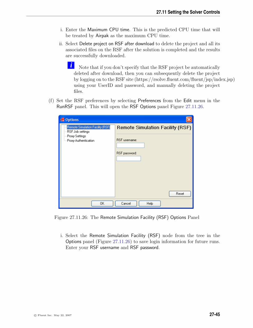
27.11 Setting the Solver Controls
i. Enter the Maximum CPU time. This is the predicted CPU time that willbe treated by Airpak as the maximum CPU time.
ii. Select Delete project on RSF after download to delete the project and all itsassociated files on the RSF after the solution is completed and the resultsare successfully downloaded.
i Note that if you don’t specify that the RSF project be automaticallydeleted after download, then you can subsequently delete the projectby logging on to the RSF site (https://rsolve.fluent.com/fluent/jsp/index.jsp)using your UserID and password, and manually deleting the projectfiles.
(f) Set the RSF preferences by selecting Preferences from the Edit menu in theRunRSF panel. This will open the RSF Options panel Figure 27.11.26.
Figure 27.11.26: The Remote Simulation Facility (RSF) Options Panel
i. Select the Remote Simulation Facility (RSF) node from the tree in theOptions panel (Figure 27.11.26) to save login information for future runs.Enter your RSF username and RSF password.
c© Fluent Inc. May 22, 2007 27-45

Calculating a Solution
ii. Select the RSF Job settings node from the tree (Figure 27.11.27) to set theRSF job settings. Select Delete project on RSF after download to deletethe project and all its associated files on the RSF after the solution iscompleted and the results are successfully downloaded.
Enter the Airpak Application Id to identify the version of Airpak that youwant to run on your project (e.g., 2112 for Airpak 2.1.12). By default,the latest version of Airpak will be run.
i Note that if you don’t specify that the RSF project be automati-cally deleted after download, then you can subsequently log on to theRSF site (https://rsolve.fluent.com/fluent/jsp/index.jsp) using yourUserID and password, and manually delete the project.
Figure 27.11.27: The RSF Job settings Panel
27-46 c© Fluent Inc. May 22, 2007

27.11 Setting the Solver Controls
iii. Select the Proxy settings node in the tree (Figure 27.11.28) to configurethe proxy to access the RSF. Enter the server and server port information.Select Use a proxy server to access the Internet to access the Internet usinga proxy server.
Figure 27.11.28: The Proxy Settings Panel
c© Fluent Inc. May 22, 2007 27-47

Calculating a Solution
iv. Select the Proxy Authentication node in the tree (Figure 27.11.29) to setthe proxy parameters. Select the Authentication type from the drop-downlist and enter the User name, Password, and Domain. The Reset buttonallows you to return to your original settings.
Figure 27.11.29: The Proxy Authentication Panel
v. Click OK in the Options panel to save the preferences you have set foryour RSF solution and close the panel.
(g) To start the solution on the RSF, click the Start Solution button in the Maintab of the RunRSF panel (Figure 27.11.21). This will open the Connect toRemote Simulation Facility panel (Figure 27.11.30).
Figure 27.11.30: The Connect to Remote Simulation Facility panel
(h) Follow Step 3 of the previous procedure for running RSF from within Airpak tolog on to RSF, run your solution, and download your results for postprocessing.
27-48 c© Fluent Inc. May 22, 2007

27.12 Performing Calculations
27.12 Performing Calculations
The following sections provide information about what Airpak does when a calculationis started, during the calculation, and when the calculation ends. Information is alsoprovided about judging the convergence of your solution.
27.12.1 Starting the Calculation
When you click on the Start solution button in the Solve panel (Figure 27.11.1), Airpakperforms various preprocessing operations, including checking the model, saving a projectfile, and creating a case file for the solver. The solver will then begin to calculate. SeeSection 31.6 for theoretical information on the solution procedures.
If Show diagnostic output from solver is selected in the Solve panel (the default setting), aseparate window will open and the solver will print the numeric values of the residualsto the window.
If Start monitor is selected in the Solve panel (the default setting), Airpak will displaythe convergence history for the calculation in the Solution residuals graphics display andcontrol window. See Section 27.12.2 for details on the Solution residuals graphics displayand control window.
If Enable sequential solution of flow and energy equations is selected in the Solve panel,Airpak will first solve the flow equations, and then solve the energy equation alone. SeeSection 27.11.2 for details.
The solver runs as a background task separate from Airpak, so you can work on anothermodel once the solver starts to solve the current model.
Airpak will save the results of the calculation for non-transient problems at the frequencyspecified next to Auto-save interval in the Solve panel. See Section 27.11.2 for details.For a transient simulation, Airpak will save the results at the frequency specified next toSolution save interval in the Transient parameters panel, as described in Section 20.1.
27.12.2 The Solution residuals Graphics Display and Control Window
Airpak opens the Solution residuals graphics display and control window (Figure 27.12.1)by default when the solver starts to perform calculations, and displays the convergencehistory for the calculation.
The Solution residuals window is fully interactive. For example, at any time during thecalculation, you can zoom in on a specific portion of the graph. To zoom into an area,position the mouse pointer at a corner of the area to be zoomed, hold down the left mousebutton and drag open a selection box to the desired size, and then release the mousebutton. The selected area will then fill the Solution residuals window, with appropriatechanges to the axes. After you have zoomed into an area, click on Full range to restorethe graph to its original axes and scale.
c© Fluent Inc. May 22, 2007 27-49

Calculating a Solution
Figure 27.12.1: The Solution residuals Graphics Display and Control Window
27-50 c© Fluent Inc. May 22, 2007

27.12 Performing Calculations
Other options available in the Solution residuals window include the following:
X log converts the horizontal axis to a logarithmic scale.
Y log converts the vertical axis to a logarithmic scale.
Symbols displays data points on the plotted line.
Lines displays the plotted line.
X grid displays the vertical grid lines on the plot.
Y grid displays the horizontal grid lines on the plot.
Done cancels the monitor and closes the Solution residuals window, but does not ter-minate the solver.
Lower pri changes the solver to a lower priority on the machine permanently for theduration of the calculation.
Terminate stops the solver project after the current iteration is completed. Airpakacknowledges the termination request in the Message window, but the solver doesnot stop until the Solution (projectname) is finished message appears. Notethat the Terminate button does not close the Solution residuals window.
Print generates a hardcopy of the residuals in the Solution residuals window. SeeSection 3.5 for details on saving an image file.
Set range allows you to specify a range for the values of a variable at a monitor point.
Full range allows you to restore the graph to its original axes and scale, if you haveused the Set range option.
i Note that you can change the solution-residual display in the Solution residualswindow during the calculation, as described in Section 27.12.3.
27.12.3 Changing the Solution Monitors During the Calculation
During the calculation, Airpak will update the solution residuals and point monitors aftereach iteration. You can change the display of the convergence monitors while the solveris running using the Solution monitor definition panel.
Solve−→Solution monitor
This panel is very similar to the Solution monitor parameters panel (see Figure 27.8.1).You can also specify a Solution ID of the solver calculation you wish to monitor in theSolution monitor definition panel. The default Solution ID will correspond to the solution
c© Fluent Inc. May 22, 2007 27-51

Calculating a Solution
ID for the current calculation when the solver is running. You can make changes to theSolution monitor definition panel while the solver is running. Click Create to make thechanges appear in the Solution residuals graphics display and control windows.
27.12.4 Ending the Calculation
The solution will stop after the specified number of iterations or if the convergencecriteria are met. You can also stop the solver during the calculation using the Terminatebutton in the Monitor window (see Section 27.12.2 for details). The message Solution
(projectname) is finished appears in the Message window when the solver is done.Note that the Solution residuals windows will remain open until you close them by clickingDone.
If Write overview of results when finished is selected in the Solve panel, Airpak will generatean overview of results when it has finished the calculation.
If Write report when finished is selected in the Solve panel, Airpak will generate the report(s)that you defined in the Define summary report panel (see Section 27.10).
If Compress solution after reporting is selected in the Solve panel, Airpak will compresssome solver-related files when it has finished the calculation to reduce the usage of diskspace. This will not affect postprocessing of the solution.
If Export solution data is selected in the Solve panel, Airpak will export the solution datato the file specified in the Export solution data text entry box (see Section 27.11.2 fordetails).
27.12.5 Judging Convergence
There are no universal metrics for judging convergence. Residual definitions that areuseful for one class of problem are sometimes misleading for other classes of problems. Formost Airpak models, the default convergence criterion is sufficient. This criterion requiresthat the scaled residuals defined by Equations 31.6-42 and 31.6-44 in Section 31.6.5decrease to 10−3 for all equations except the energy equation, for which the criterion is10−7.
27.13 Diagnostic Tools for Technical Support
Airpak includes a number of tools designed to aid your technical support engineer introubleshooting problems in the solver execution. These tools are intended for diagnosticpurposes only. The Diagnostics sub-menu provides access to these tools. To open theDiagnostics sub-menu, select Diagnostics in the Solve menu.
Solve−→Diagnostics
The following options are available for diagnostic purposes.
27-52 c© Fluent Inc. May 22, 2007

27.13 Diagnostic Tools for Technical Support
Edit .cas file opens a text-editor window in which you can edit the case file that con-tains the model information used by the solver.
Edit .diag file opens a text-editor window in which you can edit or view the diagnosticfile created for input to the solver. Typically, this will be of use to your technicalsupport engineer in diagnosing the problem.
Edit .uns out file opens a text-editor window in which you can edit or view the residualsfile created by the solver. This is useful to either check the amount of time taken bythe solver, or to check for any errors printed out during the course of the solution.
Edit Optimization log opens a text-editor window in which you can edit or view the op-timization log created by Airpak. This is useful to get detailed information regardingthe optimization run. The quantities reported are the values of design variables forall trials performed, the corresponding objective and constraint functions, and therelative changes in each of these quantities.
To combine all relevant files for your model into a single file that you can send to yourtechnical support engineer, select Pack from the File menu.
File−→Pack
This opens the File selection dialog box, in which you can select a name for the packagedfile. See Section 2.1.8 for details on selecting a file.
To email the packaged project, select Email project from the File menu.
File−→Email project
This will open the File selection dialog box, in which you can select a name for thepackaged file. See Section 2.1.8 for details on selecting a file. By clicking the Save buttonin the File selection dialog box, the Email Project panel will open up (Figure 27.13.1). Inthis panel enter Recipient email address, Subject for email, and Message text, then clickSend email.
Figure 27.13.1: The Email Project Panel
c© Fluent Inc. May 22, 2007 27-53

Calculating a Solution
27-54 c© Fluent Inc. May 22, 2007

Chapter 28. Examining the Results
Airpak provides a number of different methods for examining the results of your simulation(also referred to as postprocessing your results). You can create graphical displays of dataon different portions of the model, or two-dimensional (XY) plots of solution data.
The information in this chapter is divided into the following sections:
• Section 28.1: Overview: The Post Menu and Postprocessing Toolbar
• Section 28.2: Graphical Displays
• Section 28.3: XY Plots
• Section 28.4: Selecting a Solution Set to be Examined
• Section 28.5: Zoom-in Modeling
28.1 Overview: The Post Menu and Postprocessing Toolbar
28.1.1 The Post Menu
The Post menu is accessible from the Main Menu bar. When you select Post in the MainMenu bar, a set of options is displayed as shown in Figure 28.1.1.
The Post menu contains all of the functions you need to examine your results in Airpak.These functions include the following:
• displaying results on one or more faces of an object (Post−→Object face)
• displaying results on a cross-section of the model (Post−→Plane cut)
• displaying results on an isosurface (Post−→Isosurface)
• displaying results at a point (Post−→Point)
• displaying results at a point on a surface (Post−→Surface probe)
• displaying the locations of the minimum and maximum values of postprocessingvariables (Post−→Min/max locations)
• plotting a variable along a line through the model (Post−→Variation plot)
c© Fluent Inc. May 22, 2007 28-1

Examining the Results
Figure 28.1.1: The Post Menu
28-2 c© Fluent Inc. May 22, 2007

28.1 Overview: The Post Menu and Postprocessing Toolbar
• plotting a variable over different solutions (Post−→Trials plot)
• selecting a specific solution set to be examined (Post−→Load solution ID)
• loading postprocessing objects from a file (Post−→Load post object from file)
• saving postprocessing objects to a file (Post−→Save post objects to file)
• rescaling vectors to their original sizes (Post−→Rescale vectors)
• creating zoom-in models (Post−→Create zoom-in model)
In addition to these functions, the Post menu contains options for plotting solution resid-uals (Post−→Convergence plot, described in Chapter 27), solution variable histories overtime (Post−→History plot, described in Chapter 20). Functions for units (Post−→Post-processing units) and transient simulations (Post−→Transient settings) are described inChapters 5 and 20, respectively. The time-averaging function (Post−→Time average) fortransient results is described in Chapter 20. The function for downloading your RSF-runproject for postprocessing (Post−→Download RSF project) is described in Section 27.11.5.
If you have saved any postprocessing objects in your project file using the Save postpro-cessing objects option in the Save project panel (as described in Section 3.4), Airpak willask you if you want to load them when you enter the Post menu for the first time.
c© Fluent Inc. May 22, 2007 28-3
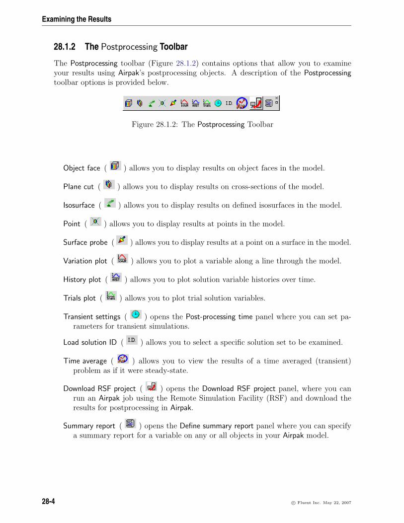
Examining the Results
28.1.2 The Postprocessing Toolbar
The Postprocessing toolbar (Figure 28.1.2) contains options that allow you to examineyour results using Airpak’s postprocessing objects. A description of the Postprocessingtoolbar options is provided below.
Figure 28.1.2: The Postprocessing Toolbar
Object face ( ) allows you to display results on object faces in the model.
Plane cut ( ) allows you to display results on cross-sections of the model.
Isosurface ( ) allows you to display results on defined isosurfaces in the model.
Point ( ) allows you to display results at points in the model.
Surface probe ( ) allows you to display results at a point on a surface in the model.
Variation plot ( ) allows you to plot a variable along a line through the model.
History plot ( ) allows you to plot solution variable histories over time.
Trials plot ( ) allows you to plot trial solution variables.
Transient settings ( ) opens the Post-processing time panel where you can set pa-rameters for transient simulations.
Load solution ID ( ) allows you to select a specific solution set to be examined.
Time average ( ) allows you to view the results of a time averaged (transient)problem as if it were steady-state.
Download RSF project ( ) opens the Download RSF project panel, where you canrun an Airpak job using the Remote Simulation Facility (RSF) and download theresults for postprocessing in Airpak.
Summary report ( ) opens the Define summary report panel where you can specifya summary report for a variable on any or all objects in your Airpak model.
28-4 c© Fluent Inc. May 22, 2007

28.2 Graphical Displays
28.2 Graphical Displays
28.2.1 Overview of Generating Graphical Displays
Airpak allows you to view solution results for the variables listed in Chapter 30 in fourtypes of locations in the domain:
• on one or more faces of a selected object in the model (e.g., the side of a PCB orthe face of a block)
• on a cross-sectional plane that extends throughout the room or a truncated plane
• on a surface (called an isosurface) defined by the constant value of a specifiedvariable, such as temperature
• at a particular point in the model, which can be easily moved to examine resultsat various locations
Sections 28.2.4–28.2.7 describe how to display results on these four types of locations inthe model, which are referred to as postprocessing objects. Section 28.2.3 describes howto manage these postprocessing objects (e.g., how to delete, deactivate, and save them).
In the specified portion of the domain, you can display the data in four ways:
• contours of a specified variable, such as temperature or pressure
• vectors of a specified variable
• particles released from the object or surface
• mesh on the specified object or surface in a specified color
Parameters that control contour, vector, and particle displays are described in Sec-tions 28.2.8–28.2.10.
28.2.2 The Significance of Color in Graphical Displays
Contour, vector, and particle displays are associated with a color spectrum representingthe range of values for the variable being displayed (e.g., temperature). The spectrumranges from violet (minimum value) to red (maximum value).
Airpak displays a legend (in the graphics window) showing the color spectrum and itsassociated values for the currently-selected postprocessing object. To reposition the leg-end, hold down the <Control> key, press and hold down the middle mouse button, anddrag the legend to any location in the graphics window.
c© Fluent Inc. May 22, 2007 28-5

Examining the Results
The default color spectrum is evenly distributed across the range of values for the specifiedvariable (i.e., each band of the color spectrum is associated with an equal portion of thevariable range). It is possible, however, to change the ranges in order to increase ordecrease the size of the color band associated with a particular portion of the variablerange. To do so, hold down the <Control> key, press and hold down the right mousebutton, and drag the legend value lines up or down the spectrum. To return the legendto its original appearance, select Rescale vectors in the Post menu.
You can change the format of the labels that define the color divisions in the legend usingthe Settings panel. See Section 6.3 for details of the data formats available in Airpak, andhow to specify the precision for each of the available formats.
28.2.3 Managing Postprocessing Objects
Once you have created postprocessing objects (according to the instructions in Sec-tions 28.2.4–28.2.7), you can manipulate them using the Postprocessing node in the Modelmanager window, shown in Figure 28.2.1.
Figure 28.2.1: The Post-processing Node in the Model manager Window
When you define a new postprocessing object using one of the options in the Post menuor Postprocessing toolbar (i.e., Object face, Plane cut, Isosurface, Surface probe, or Point),the object is added under the Postprocessing node in the Model manager window. As isthe case for modeling objects, each postprocessing object has a unique object name, suchas iso.1. In the Model manager window shown in Figure 28.2.1, for example, one of eachtype of postprocessing object is listed.
Summary data associated with the postprocessing object selected in the Model managerwindow is displayed in the Edit window (Figure 28.2.2). The values displayed are theglobal and object-specific minima and maxima, location of the maximum of the variablethat is being plotted, total, mean, and standard deviation of the variable, and area ofthe postprocessing object (or a value of the specified variable and the location for a pointobject). You can save the object’s summary information listed in the Edit window, byclicking the Save button. This will open the Save summary data panel, in which you canselect or specify the name of your summary file.
28-6 c© Fluent Inc. May 22, 2007

28.2 Graphical Displays
Figure 28.2.2: The Edit Window for postprocessing objects
The following sections describe the ways in which you can manipulate postprocessingobjects.
Activating and Deactivating Postprocessing Objects
By default, all postprocessing objects that you create will remain in the graphics window.If you have created several postprocessing objects, the display can become very cluttered,making it difficult to examine your results carefully. In such cases, you can remove anobject from the display temporarily by selecting it in the Model manager window, right-clicking to open the context menu, and turning off the Active option. You can repeat thisfor each object that you do not want to include in the display. You can also deactivate anobject by selecting it in the Model manager window and dragging it to the Inactive nodein the Model manager window. When an object is deactivated, it is simply removed fromthe display, not deleted from Airpak. Since it still exists, you can add it to the displayagain by turning the Active option back on, or by dragging the object from the Inactivenode into the Postprocessing node of the Model manager window.
Modifying Postprocessing Objects
If you want to modify an existing postprocessing object (e.g., select different faces ofan object for display), double-click on the postprocessing object in the Model managerwindow, or right-click on the postprocessing object and select the Edit option in thecontext menu. Airpak will open the appropriate panel (e.g., the Object face or Isosurfacepanel), where you can make the desired changes to the object.
Deleting Postprocessing Objects
To delete a postprocessing object, select the object in the Model manager window and
click the button. The object will be removed from the display. Alternatively, youcan right-click on the selected object in the Model manager window and select Delete from
c© Fluent Inc. May 22, 2007 28-7

Examining the Results
the drop-down list. You can also drag the selected postprocessing object into the Trashnode of the Model manager window.
i Unlike other Airpak objects, postprocessing objects are permanently deleted whena delete operation is performed.
Rescaling Vectors in the Display
If one or more postprocessing objects include vectors, zooming in or out on the displaywill cause both the model and the vectors to increase or decrease in size. To redisplaythe model with the vectors drawn at their original sizes, select Rescale vectors in the Postmenu.
Saving and Reloading Postprocessing Objects
After creating a number of postprocessing objects, you may want to save them to a fileso that you can reuse them the next time you view this model in Airpak. To save allexisting postprocessing objects to a file, select Save post objects to file in the Post menu.Enter a name in the File name text field in the resulting File selection dialog box, andclick Save to save the file.
To read the postprocessing objects back into Airpak, select Load post objects from file inthe Post menu. Enter the appropriate file name in the File name text field in the resultingFile selection dialog box, and click Open to load the objects from the file.
Saving, Reloading, and Clearing Airpak Views
After obtaining a certain Airpak view during postprocessing, you may want to save theview so that you can revisit it at a later time during your Airpak session. To save anAirpak view, select Save user view in the Orient menu. Airpak will open a Query panel,prompt you for a view name, and save the current view using your specified name. Thenew view name is attached to the list of user views at the bottom of the Orient menu.To reload the view back into Airpak at a later time during the same session, select theview name listed at the bottom of the Orient menu. To remove all saved views from thelisting, select Clear user views in the Orient menu.
i Note that views are only temporarily saved during a particular Airpak work session.The views are not saved when you quit Airpak.
28-8 c© Fluent Inc. May 22, 2007
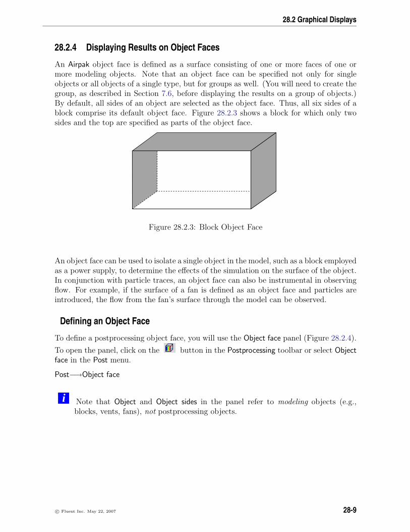
28.2 Graphical Displays
28.2.4 Displaying Results on Object Faces
An Airpak object face is defined as a surface consisting of one or more faces of one ormore modeling objects. Note that an object face can be specified not only for singleobjects or all objects of a single type, but for groups as well. (You will need to create thegroup, as described in Section 7.6, before displaying the results on a group of objects.)By default, all sides of an object are selected as the object face. Thus, all six sides of ablock comprise its default object face. Figure 28.2.3 shows a block for which only twosides and the top are specified as parts of the object face.
Figure 28.2.3: Block Object Face
An object face can be used to isolate a single object in the model, such as a block employedas a power supply, to determine the effects of the simulation on the surface of the object.In conjunction with particle traces, an object face can also be instrumental in observingflow. For example, if the surface of a fan is defined as an object face and particles areintroduced, the flow from the fan’s surface through the model can be observed.
Defining an Object Face
To define a postprocessing object face, you will use the Object face panel (Figure 28.2.4).
To open the panel, click on the button in the Postprocessing toolbar or select Objectface in the Post menu.
Post−→Object face
i Note that Object and Object sides in the panel refer to modeling objects (e.g.,blocks, vents, fans), not postprocessing objects.
c© Fluent Inc. May 22, 2007 28-9

Examining the Results
Figure 28.2.4: The Object face Panel
The procedure for defining an object face is as follows:
1. In the Name field, enter a new name for the object face. The default name is face.n,where n is a sequential number distinct for each object face created. You can keepthe default name if you want, but a customized name is generally more useful.
2. To select the specific modeling object for which you want to create an object face,select the desired object (e.g., vent.1) in the Object drop-down list. The objectname is displayed in the text field. (e.g., object vent.1).
3. To specify more than one object for which you want to create the object face,select the desired object (e.g., vent.1) from the Object drop-down list, hold downthe <Control> key, and select another object from the list. When multiple objectsare selected, the object names are listed in the Object text field separated by spaces.
To select multiple items that are listed consecutively in the drop-down list, you canselect the first item, hold down the <Shift> key, and then select the last item inthe list. All items between the first selected item and the last selected item will beselected.
4. Specify which sides of the modeling object should be included in the object faceby enabling/disabling the corresponding options for Object sides. Only those sidesappropriate for the object selected in the Object list will be available. Rectangular-block specifications, for example, include Min X, Max X, Min Y, Max Y, Min Z, and
28-10 c© Fluent Inc. May 22, 2007

28.2 Graphical Displays
Max Z. Cylindrical and polygonal blocks, on the other hand, include Top, Bottom,and Sides. (For a rectangular block, Min X and Max X represent the sides of theblock on the x axis with the minimum and maximum x values, respectively.) Bydefault, all object sides are active.
5. Specify which type of display you want to show on the object face by turning onthe appropriate option: Show mesh, Show contours, Show vectors, or Show particletraces. (You can choose more than one, but the resulting display may become toobusy.)
6. To modify the default attributes of a contour, vector, or particle display, click thecorresponding Parameters button. See Sections 28.2.8–28.2.10 for details. If youchoose to display the mesh, you can specify the mesh color by selecting a color inthe drop-down color palette. To display the color palette, click on the small colorrectangle next to the Show mesh option.
7. Click Define to define the object face according to the specifications in the panel,without loading the data. If the data had already been loaded, this button will becalled the Display button. The Define (or Display) button will change to the Updatebutton, which you can use to update the object face if you make further changesto the specifications in the panel. To create and display the object face by loadingthe data, click the Create button.
Modifying an Existing Object Face
If you want to modify an existing object face, make the desired changes to the entries inthe Object face panel, and then click Update. If you start to make changes but then wishto return to the original settings in the panel, click Reset. Airpak will update the panelwith the settings that were last saved (i.e., the settings that were present when you lastclicked Create, Update, or Done).
Creating Another Object Face
If you are already in the Object face panel and you want to create a new object face, clickNew at the bottom of the panel. Airpak will increment the number on the default Nameand clear the previous settings so that you can start defining a new object face.
Deactivating or Deleting an Object Face
If you want to temporarily remove the object face from the display, you can turn off theActive option at the top of the Object face panel. This has the same effect as turning offthe Active option in the postprocessing object context menu, described in Section 28.2.3.
c© Fluent Inc. May 22, 2007 28-11
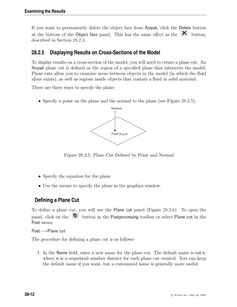
Examining the Results
If you want to permanently delete the object face from Airpak, click the Delete button
at the bottom of the Object face panel. This has the same effect as the button,described in Section 28.2.3.
28.2.5 Displaying Results on Cross-Sections of the Model
To display results on a cross-section of the model, you will need to create a plane cut. AnAirpak plane cut is defined as the region of a specified plane that intersects the model.Plane cuts allow you to examine areas between objects in the model (in which the fluidalone exists), as well as regions inside objects that contain a fluid or solid material.
There are three ways to specify the plane:
• Specify a point on the plane and the normal to the plane (see Figure 28.2.5).
Point (x,y,z)
Normal
Figure 28.2.5: Plane Cut Defined by Point and Normal
• Specify the equation for the plane.
• Use the mouse to specify the plane in the graphics window.
Defining a Plane Cut
To define a plane cut, you will use the Plane cut panel (Figure 28.2.6). To open the
panel, click on the button in the Postprocessing toolbar or select Plane cut in thePost menu.
Post−→Plane cut
The procedure for defining a plane cut is as follows:
1. In the Name field, enter a new name for the plane cut. The default name is cut.n,where n is a sequential number distinct for each plane cut created. You can keepthe default name if you want, but a customized name is generally more useful.
28-12 c© Fluent Inc. May 22, 2007

28.2 Graphical Displays
Figure 28.2.6: The Plane cut Panel
2. Define the plane using one of the following four methods:
• Specify a plane through the center of the model:
(a) Select X plane through center, Y plane through center, or Z plane throughcenter in the Set position drop-down list under Plane location in the Planecut panel. The plane cut created is perpendicular to the specified axis.For example, selecting Y plane through center creates a plane in the x-zplane located in the center of the model.
• Specify a point on the plane and the normal direction to the plane:
(a) Select Point and normal in the Set position drop-down list.
(b) Enter the coordinates of a point on the plane (PX, PY, PZ).
(c) Enter a vector defining the direction normal to the plane (NX, NY, NZ).For example, entering (1, 0, 0) for the vector will define a normal pointingin the x direction.
• Specify an equation that defines the plane:
(a) Select Coeffs (Ax + By + Cz = D) in the Set position drop-down list.
(b) Enter the coefficients A, B, C, and D for the equation
Ax+By + Cz = D (28.2-1)
c© Fluent Inc. May 22, 2007 28-13

Examining the Results
• Specify the plane using your mouse:
(a) Use the Orient menu or the Orientation commands toolbar to specify thedesired orientation. If you require a horizontal or vertical plane throughyour model, choose the orientation such that the plane of the displayscreen is perpendicular to the desired plane cut. For example, if you wantto display results on a y-z or x-y plane, choose Orient positive Y as theorientation so that the display-screen plane is the x-z plane. If you wantto specify the plane by selecting three points on it, orient your model asdesired.
(b) Select Horizontal-screen select, Vertical-screen select, or 3 Points-screen se-lect in the Set position drop-down list in the Plane cut panel.
(c) If you selected the Horizontal-screen select or Vertical-screen select option,click your left mouse button in the graphics window to indicate a pointon the desired plane. Airpak will create a plane cut that is a horizontalor vertical plane perpendicular to the plane of the graphics window andpassing through the selected point.
If you selected the 3 Points-screen select option, select the first, second,and third points on the plane in the graphics window using the left mousebutton. Each point must be on the edge of an object or the room. If it isnot, Airpak will move the point to the nearest location on the edge of anobject or the room.
i The procedure for defining the plane cut with your mouse is the sameas for defining a plane for displaying the mesh. See Section 26.9.2 foradditional information (including diagrams).
3. Specify which type of display you want to show on the plane cut by turning onthe appropriate option: Show mesh, Show contours, Show vectors, or Show particletraces. You can choose more than one, but the resulting display may become toobusy.
4. To modify the default attributes of a contour, vector, or particle display, click thecorresponding Parameters button. See Sections 28.2.8–28.2.10 for details. If youchoose to display the mesh, you can specify the mesh color by selecting a colorin the drop-down color palette. To display the color palette, click the small colorrectangle next to the Show mesh option.
5. Click Define to define the plane cut according to the specifications in the panel,without loading the data. If the data had already been loaded, this button will becalled the Display button. The Define (or Display) button will change to the Updatebutton, which you can use to update the plane cut if you make further changes tothe specifications in the panel. To create and display the plane cut by loading thedata, click the Create button.
28-14 c© Fluent Inc. May 22, 2007

28.2 Graphical Displays
6. To advance the currently-displayed plane cut through the room so that you caneasily view results on different cross-sectional planes, use the slider bar under Planelocation. You can also generate an animation of the plane cut moving through theroom, as described below.
Modifying an Existing Plane Cut
If you want to modify an existing plane cut, make the desired changes to the entries inthe Plane cut panel, and then click Update. If you start to make changes but then wishto return to the original settings in the panel, click Reset. Airpak will update the panelwith the settings that were last saved (i.e., the settings that were present when you lastclicked Create, Update, or Done).
Creating Another Plane Cut
If you are already in the Plane cut panel and you want to create a new plane cut, clickNew at the bottom of the panel. Airpak will increment the number on the default Nameand clear the previous settings so that you can start defining a new plane cut.
Animating a Plane Cut
If you want to create an animation that progresses from one static view of a plane cut tothe next, go to the Animation section of the Plane cut panel (Figure 28.2.6).
To create an animation showing how relevant contours, vectors, particle displays, and/orthe mesh change as you move through the room, follow the steps below.
1. Specify the starting plane cut (Start) and the ending plane cut (End) for the ani-mation. A Start of 0 and an End of 1 indicates that the animation will begin atone end of the room and finish at the opposite end. The direction of the animationthrough the room is defined by the direction of the normal to the plane specifiedin the Plane cut panel.
2. Specify the number of steps (Steps), i.e., the number of plane cuts Airpak shoulddisplay between the starting plane and the ending plane. Airpak will interpolatesmoothly between the starting plane and the ending plane that you define, creating
c© Fluent Inc. May 22, 2007 28-15

Examining the Results
the specified number of planes. Note that the number of steps includes the startingand ending planes.
3. Specify the Delay (ms) or the time between each frame in the animation in mil-liseconds. This will determine the duration of the animation. For example, if youspecify 10 plane cuts next to Steps, and then specify 500 as the Delay (ms), Airpakwill create a five-second animation of the plane cuts. Note that the delay value isadded to however long it takes Airpak to create a snapshot for the animation. Thetime it takes Airpak to create a snapshot is dependent on the speed of your system.
4. If you want Airpak to play the animation only in the graphics window, and youwant the playback to repeat continuously, turn on the Loop mode option. To playthe animation once through from start to finish, turn off the Loop mode option.You can also use the Loop mode option if you want to save an animated GIF orFLI file, as described below.
5. To save the animation to a file, select the Write to file option and click the Writebutton. This displays the Save animation file selection dialog box where you cansave animations in MPEG, AVI, animated GIF, FLI, or Flash format. See belowfor details about saving animations.
Note that when the Write to file option is selected, the Delay (ms) field becomesthe Frames/s field. The Frames/s field designates the number of animation framesdisplayed per second.
6. Click Animate to start the animation. To stop the animation during playback, clickthe Interrupt button in the upper right hand corner of the Airpak interface.
Saving an Animation
You can save an animation to an MPEG, AVI, animated GIF, FLI, or Flash file usingthe Save animation file selection dialog box.
In either format, there are two options for you to consider when saving an animation file:Print region and Scale factor. These options are available when you click the Options...button in the Save animation file selection dialog box.
Print region allows you to define the region of the graphics window that should be writtento the file. See Section 3.5.2 for details about specifying the Print region.
The Scale factor is the factor by which Airpak will scale the image of the graphics windowwhen it creates the file. If you specify a Scale factor of less than 1 for any of the filesdescribed below, you may want to thicken the outlines of the room and the objects in thegraphics window; otherwise these outlines might not appear in the animation file. Youcan use the Graphical styles panel (described in Section 6.3.6) to thicken the lines.
28-16 c© Fluent Inc. May 22, 2007

28.2 Graphical Displays
Saving an MPEG File
To save the animation as an MPEG file, select MPEG files (*.mpg) in the Files of typedrop-down list. Specify a file name in the File name text field and click Save. Note thatyou must specify the Scale factor for the MPEG file. If the MPEG file is to be viewed ona Windows machine, a Scale factor of 0.3 is recommended.
Airpak will play the animation in the graphics window and save each frame to a separatescratch file. It will then combine all the files into a single MPEG file that you can viewusing an MPEG player.
For MPEG files to be played properly, you must use one of the following frame rates:23.976, 24, 25, 29.97, 30, 50, 59.94, or 60.
Saving an AVI File
To save the animation as an AVI file, select AVI files (*.avi) in the Files of type drop-downlist. Specify a file name in the File name text field and click Save. You can specify a Scalefactor for the animation, as described above.
Airpak will play the animation in the graphics window and save each frame to a separatescratch file. It will then combine all the files into a single AVI file. You can then importthe AVI file into Microsoft PowerPoint and use the animation in a presentation.
Saving an Animated GIF File
To save the animation as an animated GIF file, select GIF files (*.gif) in the Files of typedrop-down list. Specify a file name in the File name text field and click Save. You canspecify a Scale factor for the animated GIF file, as described above. If you want theplayback of the animation in the GIF file to repeat continuously, select the Loop modeoption.
Airpak will play the animation in the graphics window and save each frame to a separatescratch file. It will then combine all the files into a single animated GIF file that youcan view using a web browser. You can also import the animated GIF file into MicrosoftPowerPoint and use the animation in a presentation.
Saving an Autodesk FLI File
To save the animation as an FLI file (an Autodesk animation file format), select FLI files(*.fli) in the Files of type drop-down list. Specify a file name in the File name text fieldand click Save. You can specify a Scale factor for the animation, as described above. Ifyou want the playback of the animation in the FLI file to repeat continuously, select theLoop mode option.
Airpak will play the animation in the graphics window and save each frame to a separatescratch file. It will then combine all the files into a single FLI file (e.g., movie.fli) that
c© Fluent Inc. May 22, 2007 28-17

Examining the Results
you can view using a web browser if you have an FLI viewer plug-in. It will also createan HTML file (e.g., movie.html) that can be viewed using a web browser. Airpak alsocreates Java applets that allow you to view the HTML file as an animation.
When you view the HTML file in a web browser, the following commands are available:
• To continue the animation in the chosen direction (forward or backward), use the<Space> bar on your keyboard.
• To play the animation forward, use the . key.
• To play the animation backward, use the , key.
• To reverse the direction of the animation during playback, use the r key.
• To speed up the animation, use the + key.
• To slow down the animation, use the - key.
• To return to the original animation speed, use the 0 (zero) key.
Note that Airpak also produces two additional files when it creates the FLI file: fli-
play.class and flickframe.class. All four files (e.g., movie.fli, movie.html, fli-play.class, and flickframe.class) must be present for the animation in the HTMLfile to be played back.
Saving a Flash File
To save the animation as a Flash file, select Flash files (*.swf) in the Files of type drop-down list. Specify a file name in the File name text field and click Save. You can specifya Scale factor for the animation, as described above.
Airpak will play the animation in the graphics window and save each frame to a separatescratch file. It will then combine all the files into a single Flash file. You can then importthe Flash file into Microsoft PowerPoint and use the animation in a presentation.
Clipping a Plane Cut
If you have created a plane cut, but you do not want to use the whole plane cut todisplay data, you can clip it to create a new plane cut that spans a specified subrange.The clipped plane cut consists of those points on the selected plane cut where the x, y,and z values are within the specified range.
To clip an existing plane cut, turn on the Enable clipping option in the Clip to box sectionin the Plane cut panel (Figure 28.2.6).
28-18 c© Fluent Inc. May 22, 2007

28.2 Graphical Displays
Enter values for Min X, Min Y, Min Z, Max X, Max Y, and Max Z, and click Update.
These values can also be automatically determined by aligning the appropriate edges ofthe clipped plane cut to the existing edges of objects or bounding boxes of assemblies.The procedure is similar to that described in Section 7.3.8.
For example, to set the Min X value, you would first click Min X displayed in orange inthe Plane cut panel, then click the edge in the graphics window that you want to alignwith the Min X edge of the clipped plane cut box.
Just as with other postprocessing objects, data associated with the clipped plane cutobject (e.g., specified variable as well as global and object-specific minima and maxima)are displayed in the Edit window (Figure 28.2.2), and you can save them in a file by usingthe Save button.
Deactivating or Deleting a Plane Cut
If you want to temporarily remove the plane cut from the display, you can turn off theActive option at the top of the Plane cut panel. This has the same effect as turning offthe Active option in the postprocessing object context menu, described in Section 28.2.3.
If you want to permanently delete the plane cut from Airpak, click the Delete button at
the bottom of the Plane cut panel. This has the same effect as the button, describedin Section 28.2.3.
28.2.6 Displaying Results on Isosurfaces
An isosurface is defined as a surface representing a constant value of any primary orderived solution variable, such as temperature. Isosurfaces can take virtually any shapeand are sometimes discontinuous. An example is shown in Figure 28.2.7.
An isosurface can be used to examine surfaces of constant value for a given solutionvariable. For example, an isosurface can be helpful if you are trying to determine howquantities such as temperature or pressure are convected through a model.
c© Fluent Inc. May 22, 2007 28-19

Examining the Results
Figure 28.2.7: Isosurface Example
28-20 c© Fluent Inc. May 22, 2007

28.2 Graphical Displays
Defining an Isosurface
To define an isosurface, you will use the Isosurface panel (Figure 28.2.8). To open the
panel, click on the button in the Postprocessing toolbar or select Isosurface in thePost menu.
Post−→Isosurface
Figure 28.2.8: The Isosurface Panel
The procedure for defining an isosurface is as follows:
1. In the Name field, enter a new name for the isosurface. The default name is iso.n,where n is a sequential number distinct for each isosurface created. You can keepthe default name if you want, but a customized name is generally more useful.
2. Specify the variable on which the isosurface is based. Select the desired variable(e.g., Temperature) from the Variable drop-down list. The available variables aredescribed in Chapter 30.
3. Specify the constant Value of the specified Variable that defines the isosurface.
4. Specify which type of display you want to show on the isosurface by turning onthe appropriate option: Show mesh, Show contours, Show vectors, or Show particletraces. (You can choose more than one, but the resulting display may become toobusy.)
5. To modify the default attributes of a contour, vector, or particle display, click thecorresponding Parameters button. See Sections 28.2.8–28.2.10 for details. If youchoose to display the mesh, you can specify the mesh color by selecting a color
c© Fluent Inc. May 22, 2007 28-21

Examining the Results
in the drop-down color palette. To display the color palette, click the small colorrectangle next to the Show mesh option.
6. Click Define to define the isosurface according to the specifications in the panel,without loading the data. If the data had already been loaded, this button will becalled the Display button. The Define (or Display) button will change to the Updatebutton, which you can use to update the isosurface if you make further changes tothe specifications in the panel. To create and display the object face by loading thedata, click the Create button.
Modifying an Existing Isosurface
If you want to modify an existing isosurface, make the desired changes to the entries inthe Isosurface panel, and then click Update. If you start to make changes but then wishto return to the original settings in the panel, click Reset. Airpak will update the panelwith the settings that were last saved (i.e., the settings that were present when you lastclicked Create, Update, or Done).
Creating Another Isosurface
If you are already in the Isosurface panel and you want to create a new isosurface, clickNew at the bottom of the panel. Airpak will increment the number on the default Nameand clear the previous settings so that you can start defining a new isosurface.
Animating an Isosurface
If you want to create an animation that progresses from one static view of an isosurfaceto the next, go to the Animation section of the Isosurface panel (Figure 28.2.8).
To create an animation showing how relevant contours, vectors, particle displays, and/orthe mesh change as you move through the room, follow the steps below.
1. Specify the starting isosurface (Start) and the ending isosurface (End) for the ani-mation. A Start of 20 and an End of 30 indicates that the animation will begin withthe display of an isosurface value of 20, and finish with the display of an isosurfacevalue of 30.
28-22 c© Fluent Inc. May 22, 2007

28.2 Graphical Displays
2. Specify the number of steps (Steps), i.e., the number of isosurfaces Airpak shoulddisplay between the starting value and the ending value. Airpak will interpolatesmoothly between the starting value and the ending value that you define, creatingthe specified number of isosurfaces. Note that the number of steps includes thestarting and ending isosurface values.
3. Specify the Delay (ms) or the time between each frame in the animation in mil-liseconds. This will determine the duration of the animation. For example, if youspecify 10 isosurfaces next to Steps, and then specify 500 as the Delay (ms), Airpakwill create a five-second animation of the isosurfaces. Note that the delay value isadded to however long it takes Airpak to create a snapshot for the animation. Thetime it takes Airpak to create a snapshot is dependent on the speed of your system.
4. If you want Airpak to play the animation only in the graphics window, and youwant the playback to repeat continuously, turn on the Loop mode option. To playthe animation once through from start to finish, turn off the Loop mode option.You can also use the Loop mode option if you want to save an animated GIF orFLI file, as described below.
5. To save the animation to a file, select the Write to file option and click the Writebutton. This displays the Save animation file selection dialog box where you cansave animations in MPEG, AVI, animated GIF, FLI, or Flash format. See belowfor details about saving animations.
Note that when the Write to file option is selected, the Delay (ms) field becomesthe Frames/s field. The Frames/s field designates the number of animation framesdisplayed per second.
6. Click Animate to start the animation. To stop the animation during playback, clickthe Interrupt button in the upper right hand corner of the Airpak interface.
Saving an Animation
You can save an animation to an MPEG, AVI, animated GIF, FLI, or Flash file usingthe Save animation file selection dialog box.
In either format, there are two options for you to consider when saving an animation file:Print region and Scale factor. These options are available when you click the Options...button in the Save animation file selection dialog box.
Print region allows you to define the region of the graphics window that should be writtento the file. See Section 3.5.2 for details about specifying the Print region.
The Scale factor is the factor by which Airpak will scale the image of the graphics windowwhen it creates the file. If you specify a Scale factor of less than 1 for any of the filesdescribed below, you may want to thicken the outlines of the room and the objects in thegraphics window; otherwise these outlines might not appear in the animation file. Youcan use the Graphical styles panel (described in Section 6.3.6) to thicken the lines.
c© Fluent Inc. May 22, 2007 28-23

Examining the Results
Saving an MPEG File
To save the animation as an MPEG file, select MPEG files (*.mpg) in the Files of typedrop-down list. Specify a file name in the File name text field and click Save. Note thatyou must specify the Scale factor for the MPEG file. If the MPEG file is to be viewed ona Windows machine, a Scale factor of 0.3 is recommended.
Airpak will play the animation in the graphics window and save each frame to a separatescratch file. It will then combine all the files into a single MPEG file that you can viewusing an MPEG player.
For MPEG files to be played properly, you must use one of the following frame rates:23.976, 24, 25, 29.97, 30, 50, 59.94, or 60.
Saving an AVI File
To save the animation as an AVI file, select AVI files (*.avi) in the Files of type drop-downlist. Specify a file name in the File name text field and click Save. You can specify a Scalefactor for the animation, as described above.
Airpak will play the animation in the graphics window and save each frame to a separatescratch file. It will then combine all the files into a single AVI file. You can then importthe AVI file into Microsoft PowerPoint and use the animation in a presentation.
Saving an Animated GIF File
To save the animation as an animated GIF file, select GIF files (*.gif) in the Files of typedrop-down list. Specify a file name in the File name text field and click Save. You canspecify a Scale factor for the animated GIF file, as described above. If you want theplayback of the animation in the GIF file to repeat continuously, select the Loop modeoption.
Airpak will play the animation in the graphics window and save each frame to a separatescratch file. It will then combine all the files into a single animated GIF file that youcan view using a web browser. You can also import the animated GIF file into MicrosoftPowerPoint and use the animation in a presentation.
Saving an Autodesk FLI File
To save the animation as an FLI file (an Autodesk animation file format), select FLI files(*.fli) in the Files of type drop-down list. Specify a file name in the File name text fieldand click Save. You can specify a Scale factor for the animation, as described above. Ifyou want the playback of the animation in the FLI file to repeat continuously, select theLoop mode option.
Airpak will play the animation in the graphics window and save each frame to a separatescratch file. It will then combine all the files into a single FLI file (e.g., movie.fli) that
28-24 c© Fluent Inc. May 22, 2007

28.2 Graphical Displays
you can view using a web browser if you have an FLI viewer plug-in. It will also createan HTML file (e.g., movie.html) that can be viewed using a web browser. Airpak alsocreates Java applets that allow you to view the HTML file as an animation.
When you view the HTML file in a web browser, the following commands are available:
• To continue the animation in the chosen direction (forward or backward), use the<Space> bar on your keyboard.
• To play the animation forward, use the . key.
• To play the animation backward, use the , key.
• To reverse the direction of the animation during playback, use the r key.
• To speed up the animation, use the + key.
• To slow down the animation, use the - key.
• To return to the original animation speed, use the 0 (zero) key.
Note that Airpak also produces two additional files when it creates the FLI file: fli-
play.class and flickframe.class. All four files (e.g., movie.fli, movie.html, fli-play.class, and flickframe.class) must be present for the animation in the HTMLfile to be played back.
Saving a Flash File
To save the animation as a Flash file, select Flash files (*.swf) in the Files of type drop-down list. Specify a file name in the File name text field and click Save. You can specifya Scale factor for the animation, as described above.
Airpak will play the animation in the graphics window and save each frame to a separatescratch file. It will then combine all the files into a single Flash file. You can then importthe Flash file into Microsoft PowerPoint and use the animation in a presentation.
Clipping an Isosurface
If you have created an isosurface, but you do not want to use the whole isosurface todisplay data, you can clip it to create a new isosurface that spans a specified subrange.The clipped isosurface consists of those points on the selected isosurface where the x, y,and z values are within the specified range.
To clip an existing isosurface, turn on the Enable clipping option in the Clip to box sectionof the Isosurface panel (Figure 28.2.8).
c© Fluent Inc. May 22, 2007 28-25

Examining the Results
Enter values for Min X, Min Y, Min Z, Max X, Max Y, and Max Z, and click Update.
These values can also be automatically determined by aligning the appropriate edges ofthe clipped isosurface to the existing edges of objects or bounding boxes of assemblies.The procedure is similar to that described in Section 7.3.8.
For example, to set the Min X value, you would first click Min X displayed in orange inthe Isosurface panel, then click the edge in the graphics window that you want to alignwith the Min X edge of the clipped isosurface box.
Just as with other postprocessing objects, data associated with the clipped isosurface ob-ject (e.g., specified variable as well as global and object-specific minimum and maximumvalues) are displayed in the Edit window (Figure 28.2.2), and you can save them in a fileby using the Save button.
Deactivating or Deleting an Isosurface
If you want to temporarily remove the isosurface from the display, you can turn off theActive option at the top of the Isosurface panel. This has the same effect as turning offthe Active option in the postprocessing object context menu, described in Section 28.2.3.
If you want to permanently delete the isosurface from Airpak, click the Delete button at
the bottom of the Plane cut panel. This has the same effect as the button, describedin Section 28.2.3.
28.2.7 Displaying Results at a Point
A point is defined as a geometric location in the model and is specified either as a three-dimensional coordinate or as a mesh node number. After a point has been created, youcan move it through the model interactively (as described later in this section).
As the point is dragged through the model, its current location will be displayed and con-tinuously updated on the postprocessing objects Edit panel (described in Section 28.2.3).The value of the velocity field and the variable for which the point is defined are alsodisplayed, thereby allowing you to interactively acquire information about the solution.If you select the option to leave a trail behind the point, its path through the modelwill be clearly marked by a continuous curve, as shown in Figure 28.2.9. If the option to
28-26 c© Fluent Inc. May 22, 2007

28.2 Graphical Displays
x
y
z Initialpoint
Currentpoint
Vector
Trail
Figure 28.2.9: Point Object
display the vector is selected, the vector associated with the selected vector variable atthe point’s current location will also be shown.
If the option to display particles is selected, particle traces starting from the point willbe displayed.
A point object can be used to probe the model, either to determine the value of a solutionvariable at a specific point (e.g., the location of a thermocouple in a physical model) oras a starting point for a broader analysis.
i When using a point object, you may find it necessary to re-orient the model (e.g.,along the coordinate axes) in order to avoid visual confusion regarding the exactlocation of the point relative to the rest of the model.
Defining a Point
To define a point, you will use the Point panel (Figure 28.2.10). To open the panel, click
on the button in the Postprocessing toolbar or select Point in the Post menu.
Post−→Point
The procedure for defining a point is as follows:
1. In the Name field, enter a new name for the point. The default name is point.n,where n is a sequential number distinct for each point created. You can keep thedefault name if you want, but a customized name is generally more useful.
2. Specify the solution variable associated with the point. Select the desired variable(e.g., Temperature) from the Variable drop-down list. The available variables aredescribed in Chapter 30.
c© Fluent Inc. May 22, 2007 28-27
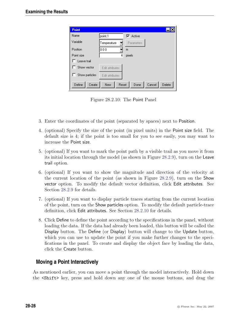
Examining the Results
Figure 28.2.10: The Point Panel
3. Enter the coordinates of the point (separated by spaces) next to Position.
4. (optional) Specify the size of the point (in pixel units) in the Point size field. Thedefault size is 4; if the point is too small for you to see easily, you may want toincrease the Point size.
5. (optional) If you want to mark the point path by a visible trail as you move it fromits initial location through the model (as shown in Figure 28.2.9), turn on the Leavetrail option.
6. (optional) If you want to show the magnitude and direction of the velocity atthe current location of the point (as shown in Figure 28.2.9), turn on the Showvector option. To modify the default vector definition, click Edit attributes. SeeSection 28.2.9 for details.
7. (optional) If you want to display particle traces starting from the current locationof the point, turn on the Show particles option. To modify the default particle-tracedefinition, click Edit attributes. See Section 28.2.10 for details.
8. Click Define to define the point according to the specifications in the panel, withoutloading the data. If the data had already been loaded, this button will be called theDisplay button. The Define (or Display) button will change to the Update button,which you can use to update the point if you make further changes to the speci-fications in the panel. To create and display the object face by loading the data,click the Create button.
Moving a Point Interactively
As mentioned earlier, you can move a point through the model interactively. Hold downthe <Shift> key, press and hold down any one of the mouse buttons, and drag the
28-28 c© Fluent Inc. May 22, 2007

28.2 Graphical Displays
point through the model in the graphics display. As the point is dragged through themodel, its current location will be displayed and continuously updated in the Edit window(described in Section 28.2.3).
Modifying an Existing Point
If you want to modify an existing point, make the desired changes to the entries in thePoint panel, and then click Update. If you start to make changes but then wish to returnto the original settings in the panel, click Reset. Airpak will update the panel with thesettings that were last saved (i.e., the settings that were present when you last clickedCreate, Update, or Done).
Creating Another Point
If you are already in the Point panel and you want to create a new point, click New at thebottom of the panel. Airpak will increment the number on the default Name and clearthe previous settings so that you can start defining a new point.
Deactivating or Deleting a Point
If you want to temporarily remove the point from the display, you can turn off the Activeoption at the top of the Point panel. This has the same effect as turning off the Activeoption in the postprocessing objects context menu, described in Section 28.2.3.
If you want to permanently delete the point from Airpak, click the Delete button at the
bottom of the Plane cut panel. This has the same effect as the button, described inSection 28.2.3.
Displaying the Value of a Variable at a Point
To display the value of a variable at a point on any postprocessing object that is displayed
in the graphics window, select Surface probe in the Post menu or click on the button.
Post−→Surface probe
Click on the postprocessing object in the graphics window using the left mouse button.Airpak will display the value of the variable at the point you selected in the graphicswindow. Additionally, the value of the variable and the coordinate location of the pointwill be printed in the Message window. If you cannot see the value in the graphicswindow, press the F9 key on the keyboard to switch the mode of the mouse to thegraphics manipulation functions described in Section 2.2.4 and then rotate the model inthe usual way. Use the F9 key to return to the Surface probe function.
c© Fluent Inc. May 22, 2007 28-29
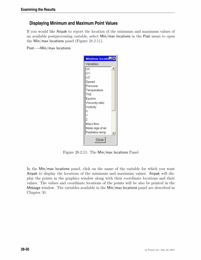
Examining the Results
Displaying Minimum and Maximum Point Values
If you would like Airpak to report the location of the minimum and maximum values ofan available postprocessing variable, select Min/max locations in the Post menu to openthe Min/max locations panel (Figure 28.2.11).
Post−→Min/max locations
Figure 28.2.11: The Min/max locations Panel
In the Min/max locations panel, click on the name of the variable for which you wantAirpak to display the locations of the minimum and maximum values. Airpak will dis-play the points in the graphics window along with their coordinate locations and theirvalues. The values and coordinate locations of the points will be also be printed in theMessage window. The variables available in the Min/max locations panel are described inChapter 30.
28-30 c© Fluent Inc. May 22, 2007

28.2 Graphical Displays
28.2.8 Contour Attributes
Contours are representations of the variation of a specified variable drawn as lines or solidbands. An individual contour follows a single value of a variable and can curve aroundor through objects. Contour plots are used to examine how a variable changes locally orthroughout the model, and are often useful for locating severe gradients and conditions(e.g., hot spots on the surfaces of objects).
Line contours (e.g., Figure 28.2.12) resemble topological maps. Solid contours can bespecified as either smooth or bands. For smooth contours the colors change in continuousgradations from one boundary of the contour to the other. For banded contours, the colorschange abruptly at the contour boundaries.
Figure 28.2.12: Contour Plot
c© Fluent Inc. May 22, 2007 28-31

Examining the Results
Overview of Defining a Contour Plot
If you have selected Show contours as the type of display to be shown on an object face,plane cut, or isosurface (in the Object face, Plane cut, or Isosurface panel), you can click theassociated Parameters button to modify the definition of the contour plot. Figure 28.2.13shows an example of the Object face contours panel.
Figure 28.2.13: The Object face contours Panel
In the Object face contours panel, the Plane cut contours panel, or the Isosurface contourspanel, you can specify the variable to be plotted, the type of contour plot (line or solid),the color levels for the plot, and several characteristics of the contour lines or solidcontours. When you are satisfied with the new settings, click Apply to see the results inthe graphics window.
Selecting the Variable to be Plotted
To choose the variable to be displayed, select the desired variable (e.g., Temperature)from the Variable drop-down list. The available variables are described in Chapter 30.
Specifying a Line or Solid Contour Plot
To specify whether you want a line contour plot or a solid contour plot (or both), turnon the Solid or Line option for Contour options. If you select both, the contours will bedisplayed as solid color bands with lines superimposed on them.
28-32 c© Fluent Inc. May 22, 2007

28.2 Graphical Displays
For line contour plots, you will specify how the line color is determined, and for solidcontour plots you will specify the shading. For both, you will also specify how the spacingor band width between contours is determined.
Constant or Variable Color for a Line Contour Plot
There are two ways to color the lines on a line contour plot. To vary the color of the linesbased on the value of the variable being plotted, select the Variable option in the Linecolor drop-down list. To have a single color for all the lines, select the Fixed option in theLine color drop-down list and then specify a color in the Color drop-down color palette.
Shading for a Solid Contour Plot
There are two ways to shade the contours on a solid contour plot. To vary the colorssmoothly in continuous gradations from one boundary of the contour to the other, selectthe Smooth option under Shading options. To have the colors change abruptly at thecontour boundaries, select the Banded option.
Specifying the Line Spacing or Band Width
For both line and solid contour plots, there are three ways to specify the line spacing orband width:
• Specify the number of contour levels or bands explicitly:
1. Select the Fixed option in the Level spacing drop-down list.
2. Enter the number of lines or bands in the Number field.
3. Specify how the maximum and minimum levels of the contour range shouldbe determined:
– To set the color levels explicitly, select Specified under Color levels andenter the Min and Max values.
– To have Airpak compute the levels for you, select Calculated, and thenchoose Global limits, This object, or Visible on screen from the drop-downlist as the method used to compute the levels. Global limits uses the max-imum and minimum values of the variable throughout the whole model.This object uses the maximum and minimum values of the variable forthe current postprocessing object only. Visible on screen uses the maxi-mum and minimum values of the variable for all postprocessing objectscurrently visible in the graphics window.
• Specify the width of the bands or the size of the interval between lines explicitly:
1. Select the Interval option in the Level spacing drop-down list.
c© Fluent Inc. May 22, 2007 28-33

Examining the Results
2. Specify the band width or the size of the interval between lines in the Incrementfield. The units for the Increment are the units of the variable being plotted.
3. Specify the minimum value for the contour range in the Start value field.
Airpak will generate subsequent intervals by repeatedly adding the Increment to theStart value.
• Specify the individual values for each line or band as discrete values of the variable:
1. Select the Input option in the Level spacing drop-down list.
2. In the field to the right of Input levels, enter the desired values for the contourlines or bands separated by spaces (e.g., 5 10 15).
You can specify as many values as you want with the Input option. If you entermore values than the text field can accommodate, the numbers entered first willdisappear at the left side of the field, but will not be lost as data. You can dragthe middle mouse button across the text field to view the hidden values at thebeginning or end of the field, or use the left and right arrows on your keyboard.
Specifying the Color Levels
The color spectrum for a line or solid contour plot is distributed across a range of valuesfor the variable being plotted. There are two ways to specify the minimum and maximumlimits for this range:
• To set the color levels explicitly, select Specified under Color levels and enter theMin and Max values.
• To have Airpak compute the color levels for you, select Calculated under Color levels,and then select Global limits, This object, or Visible on screen from the drop-downlist as the method used to compute the color levels. Global limits uses the maximumand minimum values of the variable throughout the whole model. This object usesthe maximum and minimum values of the variable for the current postprocessingobject only. Visible on screen uses the maximum and minimum values of the variablefor all postprocessing objects currently visible in the graphics window.
i Note that the selection of Specified or Calculated differs from the selection associatedwith the Fixed option for line spacing or band width. The range for the line spacingor band width indicates the minimum and maximum values that should be plotted,and the range for the color indicates the minimum and maximum values associatedwith the color spectrum. It is possible for the color range to be wider than therange of values being plotted, in which case not all colors in the spectrum will beused.
28-34 c© Fluent Inc. May 22, 2007

28.2 Graphical Displays
Saving a Contour Plot
After creating a contour plot, you can save the contour data to a file so that you canread it back into Airpak as a profile. This is useful if you have solved a large complicatedproblem and you want to zoom in to a specific region of your model and solve this regionin more detail. You can use the contour data as the boundary conditions for the regionyou want to study in more detail, and then calculate a solution only for this region.
To save contour data, create a contour plot for one of the boundaries of the region tobe studied in detail, and then click Save profile in the associated contour panel (e.g.,Figure 28.2.13). Enter a name for the contour plot in the resulting File selection dialogbox and click Accept to save the data. You can then create a wall or an opening atthe same boundary of the region to be studied in detail. To use the contour data as theboundary condition for the wall or opening, define a spatial profile on the wall or openingusing the contour data. (For information on specifying a spatial profile for an opening,see Chapter 11; for a wall, see Chapter 13.)
i Note that the shape and size of the plane containing the contour data you savedoes not have to be exactly the same shape and size as the opening or wall that youspecify. For example, if you save contour data on a plane of size 10 cm × 10 cm,and you use this data to define a boundary profile for an opening, the size of theopening does not have to be 10 cm × 10 cm. If the size of the opening is 5 cm× 5 cm, Airpak will use the contour data in this area and ignore the contour dataoutside this area. If the size of the opening is 15 cm × 15 cm, Airpak will use thecontour data at the edge of the 10 cm × 10 cm plane in the area of the openingthat is larger than 10 cm × 10 cm.
28.2.9 Vector Attributes
An Airpak postprocessing vector is an arrow, of which the length and direction representthe magnitude and direction of the velocity at a specific location in the model. Inaddition, the color of the arrow can represent the value of a scalar solution variable atthe vector location. Figure 28.2.14 shows an example vector plot.
Overview of Defining a Vector Plot
If you have selected Show vectors as the type of display to be shown on an object face,plane cut, or isosurface (in the Object face, Plane cut, or Isosurface panel), you canclick the associated Parameters button to modify the definition of the vector plot in thecorresponding vector panel (e.g., Figure 28.2.15). If you are displaying the vector at apoint, you can turn on the Show vector option and click the Edit attributes button in thePoint panel.
c© Fluent Inc. May 22, 2007 28-35

Examining the Results
Figure 28.2.14: Vector Plot
28-36 c© Fluent Inc. May 22, 2007

28.2 Graphical Displays
Figure 28.2.15: The Object face vectors Panel
In the Object face vectors panel, Plane cut vectors panel, or Isosurface vectors panel, youcan specify the distribution, color, and other characteristics of the vectors, and the colorlimits for the plot. When you are satisfied with the new settings, click Apply to see theresults in the graphics window.
Specifying the Distribution of the Vectors
By default, a vector will be displayed at each node point on the surface of the postpro-cessing object. (This is indicated by the selection of Mesh points for the Display options.)In regions where there are more mesh elements (e.g., near modeling objects), there willbe more vectors than in regions with fewer mesh elements (e.g., in open spaces). If youprefer to display vectors that are uniformly distributed, select the Uniform option forDisplay options. You can then specify the total number of vectors in the field to the rightof Uniform.
Specifying the Color of the Vectors
Vector color can be based on the magnitude of the velocity or on the value of a scalarvariable. You can also assign a single color to all vectors.
• To base the vector color on the magnitude of the velocity (the default), selectVelocity magnitude in the Color by drop-down list.
• To base the color on the value of a scalar variable, select Scalar variable in the Colorby drop-down list and then select the desired scalar variable (e.g., Temperature)
c© Fluent Inc. May 22, 2007 28-37

Examining the Results
from the Color variable drop-down list. The available variables are described inChapter 30.
• To display single-color vectors, select Fixed in the Color by drop-down list and thenspecify a color in the Fixed color drop-down color palette.
If you choose a non-fixed vector color (i.e., if you choose Velocity magnitude or Scalarvariable), the color spectrum for the vector plot will be distributed across a range ofvalues for the velocity or specified scalar variable. There are two ways to specify theminimum and maximum limits for this range:
• To set the color levels explicitly, select Specified under Color levels and enter theMin and Max values.
• To have Airpak compute the color levels for you, select Calculated under Color levels,and then select Global limits, This object, or Visible on screen from the drop-downlist as the method used to compute the color levels. Global limits uses the maximumand minimum values of the variable throughout the whole model. This object usesthe maximum and minimum values of the variable for the current postprocessingobject only. Visible on screen uses the maximum and minimum values of the variablefor all postprocessing objects currently visible in the graphics window.
Scaling the Vectors
There are two ways to scale the size of the vectors:
• Specify a scaling factor for all vectors by selecting the Factor option for Scale andentering the factor in the text field. The default factor of 1 results in a maximumvector size of approximately 1/2 inch on the screen.
• Specify a scaling factor for the largest vector by selecting the Max pixels option forScale and entering the maximum number of pixels in the text field. The size of thelargest vector on the screen will be set to the specified number of pixels, and allother vectors will be scaled proportionally.
Limiting the Display of Vectors
If there are large differences in magnitude among displayed vectors, you may want tolimit the display of the larger vectors so that you can see the smaller vectors more easily.To limit the display, enter the desired Cutoff magnitude. Any vector with a magnitudegreater than the specified Cutoff magnitude value will not be displayed.
28-38 c© Fluent Inc. May 22, 2007

28.2 Graphical Displays
Turning Off Display of Arrowheads on the Vectors
By default, the vectors are displayed with arrowheads. To display the vectors as lineswithout arrowheads, select the No arrow heads option in the Arrow style drop-down list.
28.2.10 Particle Trace Attributes
A particle trace represents the path of a hypothetical “massless” particle through themodel. The path of the particle is based on the computed flow field. Particle tracesprovide information similar to that obtained by introducing dye or smoke into the fluidof a real model. They are used primarily to observe flow in the model (e.g., to displaythe path of an air stream coming from a fan, as shown in Figure 28.2.16).
Figure 28.2.16: Particle Trace Plot
c© Fluent Inc. May 22, 2007 28-39

Examining the Results
Overview of Defining a Particle Trace Plot
If you have selected Show particle traces as the type of display to be shown on an objectface, plane cut, isosurface, or point (in the Object face, Plane cut, Isosurface, or Pointpanel), you can click the associated Parameters button to modify the definition of theparticle trace plot in the respective particles panel (e.g., Figure 28.2.17).
Figure 28.2.17: The Object face particles Panel
In the Object face particles panel, Plane cut particles panel, Isosurface particles panel, orPoint particles panel, you can specify the color of the particle traces, the frequency oftheir position calculation, their distribution, and other characteristics. When you aresatisfied with the new settings, click Apply to see the results in the graphics window.
Specifying Parameters for the Particle Position Calculation
The following parameters control the computation of the particle positions:
• The Start time specifies the time at which the particle traces begin.
• The End time specifies when the particle traces should end. Airpak estimates anend time from the time scale of the flow such that a particle introduced with the
28-40 c© Fluent Inc. May 22, 2007

28.2 Graphical Displays
highest velocity occurring in the solution will traverse the length of the enclosure.You can specify a smaller value if you want the particle traces to end before theyreach the end of the domain.
• Transient particle traces (used for transient simulations only) creates particle tracesfor a transient solution at a particular time by utilizing the velocity vector field atthat time.
• Reverse direction can be used to reverse the direction of the particle traces by tracingtheir path prior to their introduction at an object face, plane cut, isosurface, orpoint (e.g., to display the path of an air stream coming into and exiting the outletvent shown in Figure 28.2.16).
Specifying the Distribution of the Particle Traces
By default, particles traces will be uniformly distributed. (This is indicated by theselection of Uniform for the Display options.) You can specify the total number of particlesto be released in the field to the right of Uniform. If you prefer to display particles releasedfrom each node point on the surface of the postprocessing object, select the Mesh pointsoption for Display options. In regions where there are more mesh elements, there will bemore particles than in regions with fewer mesh elements.
Selecting the Display Style for the Particle Traces
Particles can be represented as discrete points or they can leave dye traces in their wake(or both).
For discrete points, select the Particles option under Style. You can then specify the Radiusof the particles in pixel units. Particle traces displayed with this option will consist ofindividual particles.
For continuous particle traces, select the Dye trace option under Style. Particle tracesdisplayed with this option will consist of a line. The width of the lines can be specifiedas integers next to Width.
Animating the Particle Traces
By default, the complete particle trace will be displayed all at once. If you want to seethe particle trace appear gradually, as the particles move through the domain, you cananimate them using the Animation section of the Object face particles panel, Plane cutparticles panel, Isosurface particles panel, or Point particles panel.
c© Fluent Inc. May 22, 2007 28-41
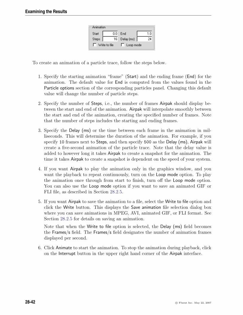
Examining the Results
To create an animation of a particle trace, follow the steps below.
1. Specify the starting animation “frame” (Start) and the ending frame (End) for theanimation. The default value for End is computed from the values found in theParticle options section of the corresponding particles panel. Changing this defaultvalue will change the number of particle steps.
2. Specify the number of Steps, i.e., the number of frames Airpak should display be-tween the start and end of the animation. Airpak will interpolate smoothly betweenthe start and end of the animation, creating the specified number of frames. Notethat the number of steps includes the starting and ending frames.
3. Specify the Delay (ms) or the time between each frame in the animation in mil-liseconds. This will determine the duration of the animation. For example, if youspecify 10 frames next to Steps, and then specify 500 as the Delay (ms), Airpak willcreate a five-second animation of the particle trace. Note that the delay value isadded to however long it takes Airpak to create a snapshot for the animation. Thetime it takes Airpak to create a snapshot is dependent on the speed of your system.
4. If you want Airpak to play the animation only in the graphics window, and youwant the playback to repeat continuously, turn on the Loop mode option. To playthe animation once through from start to finish, turn off the Loop mode option.You can also use the Loop mode option if you want to save an animated GIF orFLI file, as described in Section 28.2.5.
5. If you want Airpak to save the animation to a file, select the Write to file option andclick the Write button. This displays the Save animation file selection dialog boxwhere you can save animations in MPEG, AVI, animated GIF, or FLI format. SeeSection 28.2.5 for details on saving an animation.
Note that when the Write to file option is selected, the Delay (ms) field becomesthe Frames/s field. The Frames/s field designates the number of animation framesdisplayed per second.
6. Click Animate to start the animation. To stop the animation during playback, clickon the Interrupt button in the upper right hand corner of the Airpak interface.
28-42 c© Fluent Inc. May 22, 2007

28.3 XY Plots
Specifying the Color of the Particle Traces
Particle trace color can be based on the value of a scalar variable, or all particle tracescan be the same color.
• To base the color on the value of a scalar variable, select Scalar variable in the Colorby drop-down list and then select the desired scalar variable (e.g., Temperature) fromthe Variable drop-down list. The available variables are described in Chapter 30.
• To display single-color particle traces, select Fixed in the Color by drop-down listand specify a color in the Fixed color drop-down color palette.
If you choose a non-fixed particle color (i.e., if you choose Scalar variable or Time), thecolor spectrum for the particle trace plot will be distributed across a range of values forthe specified variable. There are two ways to specify the minimum and maximum limitsfor this range:
• To set the color levels explicitly, select Specified under Color levels and enter theMin and Max values.
• To have Airpak compute the color levels for you, select Calculated under Color levels,and then select Global limits, This object, or Visible on screen from the drop-downlist as the method used to compute the color levels. Global limits uses the maximumand minimum values of the variable throughout the whole model. This object usesthe maximum and minimum values of the variable for the current postprocessingobject only. Visible on screen uses the maximum and minimum values of the variablefor all postprocessing objects currently visible in the graphics window.
28.3 XY Plots
Airpak allows you to create four types of XY plots: convergence, history, variation, andtrials. The first two are described in Sections 27.8.1 and 20.3.5, respectively, while thevariation plot and the trials plot are described here.
28.3.1 Variation Plots
A variation plot allows you to examine a variable along any line in 3D space through themodel. Figure 28.3.1 shows an example. The distance along the line is plotted on the xaxis and the corresponding value of the variable is plotted along the y axis.
c© Fluent Inc. May 22, 2007 28-43

Examining the Results
Figure 28.3.1: Variation Plot
Generating a Variation Plot
To generate a variation plot, you will use the Variation plot panel (Figure 28.3.2). To
open the panel, click on the button in the Postprocessing toolbar or select Variationplot in the Post menu.
Post−→Variation plot
The procedure for defining a variation plot is as follows:
1. Select the variable to be plotted (e.g., Temperature) from the Variable drop-downlist. The available variables are described in Chapter 30.
28-44 c© Fluent Inc. May 22, 2007

28.3 XY Plots
Figure 28.3.2: The Variation plot Panel
2. Specify the initial point of the line (X, Y, Z) and the vector (X, Y, Z) that definesthe direction of the line. There are three methods available for defining the line:
• Enter the Point and Direction explicitly in the panel.
• Use your mouse to define the line in the graphics window:
(a) Use the Orient menu or the Orientation commands toolbar to specify thedesired orientation. Choose the orientation such that the plane of thedisplay screen is perpendicular to the desired line. For example, if youwant to display results on a line in the z direction, choose Home as theorientation so that the display-screen plane is the x-y plane.
(b) Click From screen in the Variation plot panel.
(c) Click your left mouse button in the graphics window to indicate a pointon the desired line. The resulting line will be normal to the plane of thegraphics window and pass through the selected point.
Airpak will update the Point and Direction to reflect the line definition.
• Define the line from two existing point objects:
(a) Click From point objects in the Variation plot panel.
(b) In the Model manager window, select two point objects from the Postpro-cessing node. If there are only two postprocessing point objects to choosefrom, Airpak will automatically use them. If there are more than two pointobjects, Airpak will open a Selection panel that will prompt you to choose
c© Fluent Inc. May 22, 2007 28-45

Examining the Results
two postprocessing point objects. The first point you select defines theinitial point, and the direction is defined as the vector from the first pointto the second point.
Airpak will update the Point and Direction to reflect the line definition.
3. Click Create to display the plot.
Modifying the Range of the Variation Plot
Once you have generated the variation plot, you can easily zoom in on a specific portionof the plot. To zoom on an area, position the mouse pointer at a corner of the area tobe zoomed, hold down the left mouse button and drag open a selection box window tothe desired size, and then release the mouse button. The selected area will then fill theplot window, with appropriate changes to the axes. After you have zoomed into an area,click the Full range button to restore the graph to its original axes and scale.
28-46 c© Fluent Inc. May 22, 2007

28.3 XY Plots
Modifying the Appearance of the Plot
Several options for controlling the appearance of the plot are available at the bottom ofthe plot window:
X log converts the horizontal axis to a logarithmic scale.
Y log converts the vertical axis to a logarithmic scale.
Symbols displays data points on the plotted line.
Lines displays the plotted line.
X grid displays the vertical grid lines on the plot.
Y grid displays the horizontal grid lines on the plot.
Printing the Variation Plot
If you want to print an image of the variation plot, click the Print button at the bottomof the variation plot window. See Section 3.5 for details on saving an image.
Saving and Reloading Variation Plot Data
After generating a variation plot, you may want to save the data curve to a file so thatyou can reuse it the next time you view this model in Airpak. To save variation plot datato a file, click the Save button at the bottom of the variation plot window. Enter a filename in the resulting Save curve dialog box, and click Accept to save the file.
To read the data curve back into Airpak, click the Load button at the bottom of thevariation plot window. Enter the appropriate file name in the resulting Load curve dialogbox, and click Accept to load the data.
28.3.2 Trials Plots
A trials plot allows you to compare variables at a particular point in 3D space betweendifferent solutions for the current model. In the example shown in Figure 28.3.3, the trialsolution is plotted on the x axis and the corresponding value of the variable (pressure)is plotted along the y axis. You may, however, select any variable to be plotted on the xaxis against the y axis variable, in which case the plot points will represent one variableas a function of the other at the designated point in the model domain for the specifiedtrials.
c© Fluent Inc. May 22, 2007 28-47

Examining the Results
Figure 28.3.3: Trials Plot
28-48 c© Fluent Inc. May 22, 2007

28.3 XY Plots
Generating a Trials Plot
To generate a trials plot, you will use the Trials plot panel (Figure 28.3.4). To open the
panel, click on the button in the Postprocessing toolbar or select Trials plot in thePost menu.
Post−→Trials plot
Figure 28.3.4: The Trials plot Panel
The procedure for defining a trials plot is as follows:
1. Select the variables to be plotted (e.g., Temperature) from the X Variable and YVariable drop-down lists. If you select Trial for either the x or y axis, the nameof the solutions specified below will appear as the axis label. The other availablevariables are described in Chapter 30.
2. Specify a set of solutions to compare using the Solution names field. You can typea solution name that contains an asterisk or a question mark in place of char-acters or a character, respectively. For example, typing rad* compares solutionsradiation00, radiation01, and radiation02, but not no-rad00. Typing rad?
compares solutions rad1, rad2, and rad3, but not rad10, or rad100. Use thedefault * to specify all solutions for the current model.
c© Fluent Inc. May 22, 2007 28-49

Examining the Results
3. Under Add points to plot, specify the location of the point of interest for the historyplot. There are three options:
Coords allows you to specify the coordinates of a point. Enter the X, Y, andZ coordinates and click on the Coords button. The point will appear in theList/remove points list.
Post point object allows you to select an existing point object from the Selectionpanel (Figure 28.3.5).
Figure 28.3.5: The Selection Panel
In the Selection panel, select the point in the list and click Okay. The point willappear in the List/remove points list in the History plot panel. See Section 28.2.7for details on creating a point object.
Named point allows you to select an existing named point from the point drop-down list or create a new named point. See Section 20.3.5 for details aboutcreating named points.
4. Click Create to display the XY trials plot of the selected variable(s) at the point(s)specified. Click Cancel to close the Trials plot panel without creating a trials plot.
Modifying the Range of the Trials Plot
Once you have generated the trials plot, you can easily zoom in on a specific portion ofthe plot. To zoom on an area, position the mouse pointer at a corner of the area to bezoomed, hold down the left mouse button and drag open a selection box window to thedesired size, and then release the mouse button. The selected area will then fill the plotwindow, with appropriate changes to the axes. After you have zoomed into an area, clickthe Full range button to restore the graph to its original axes and scale.
28-50 c© Fluent Inc. May 22, 2007
28.4 Selecting a Solution Set to be Examined
Modifying the Appearance of the Plot
Several options for controlling the appearance of the plot are available at the bottom ofthe plot window:
X log converts the horizontal axis to a logarithmic scale.
Y log converts the vertical axis to a logarithmic scale.
Symbols displays data points on the plotted line.
Lines displays the plotted line.
X grid displays the vertical grid lines on the plot.
Y grid displays the horizontal grid lines on the plot.
Printing the Trials Plot
If you want to print an image of the trials plot, click the Print button at the bottom ofthe trials plot window. See Section 3.5 for details on saving an image.
Saving and Reloading Trials Plot Data
After generating a trials plot, you may want to save the data curve to a file so that youcan reuse it the next time you view this model in Airpak. To save trials plot data to afile, click the Save button at the bottom of the trials plot window. Enter a file name inthe resulting Save curve dialog box, and click Accept to save the file.
To read the data curve back into Airpak, click the Load button at the bottom of the trialsplot window. Enter the appropriate file name in the resulting Load curve dialog box, andclick Accept to load the data.
28.4 Selecting a Solution Set to be Examined
If there is more than one solution set available for your model, you can specify whichsolution version you want to examine. To open the Version selection panel (Figure 28.4.1),
click on the button in the Postprocessing toolbar or select Load solution ID in thePost menu.
Post−→Load solution ID
Select the desired solution set from the list at the bottom of the panel, and click Okayto load it. The new solution will be applied automatically to the model in the graphicswindow.
c© Fluent Inc. May 22, 2007 28-51

Examining the Results
Figure 28.4.1: The Version selection Panel
28.5 Zoom-In Modeling
Airpak allows you to model sub-systems with given results from a system model using aprocess known as zoom-in or cascade modeling. This process creates a zoom-in modelwith the appropriate profiles applied automatically to the boundaries of the sub-system.
To create a zoom-in model, you will use the Zoom-in modeling panel (Figure 28.5.1). Toopen the panel, select Create zoom-in model in the Post menu.
Post−→Create zoom-in model
The procedure for creating a zoom-in model is as follows:
1. Specify a name for the zoom-in model project in the Zoom-in project text entry box.You can also click Browse next to the text field and select the desired project namein the resulting File selection dialog box. See Section 2.1.8 for more information onthe File selection dialog box.
2. Specify the solution ID of the results from the previous system model. You caneither enter the solution ID in the Solution ID text entry box, or select the solutionID using the Version selection panel. Click Select to open the Version selection panel.Note that you do not need to provide a file extension for the solution ID.
3. Specify the coordinates for each of the zoom-in model boundaries (Min X, Max X,Min Y, Max Y, Min Z, and Max Z). There are two methods available for choosingthe coordinates:
• Enter the coordinate values in the appropriate text entry boxes and press the<Enter> key on the keyboard.
• Click Select to the right of the appropriate text entry box and then click theleft mouse button on the desired point in the graphics window. You may wantto orient your view depending upon the coordinate being selected to ensure amore accurate selection.
28-52 c© Fluent Inc. May 22, 2007
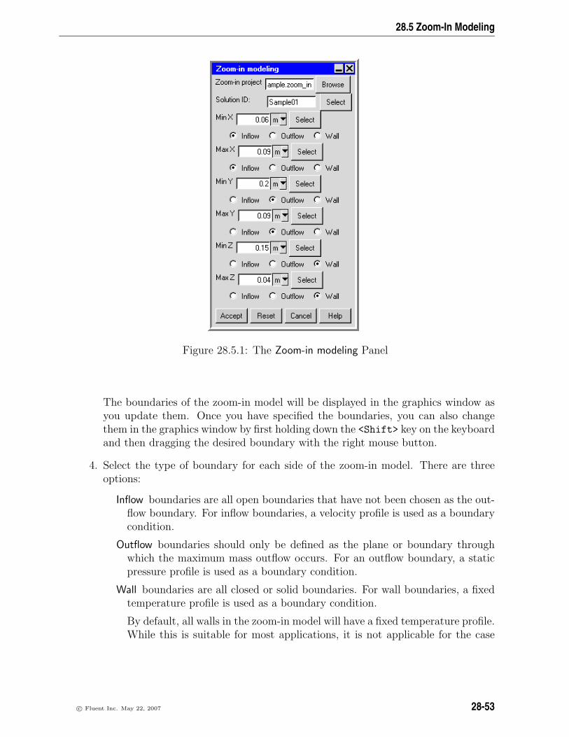
28.5 Zoom-In Modeling
Figure 28.5.1: The Zoom-in modeling Panel
The boundaries of the zoom-in model will be displayed in the graphics window asyou update them. Once you have specified the boundaries, you can also changethem in the graphics window by first holding down the <Shift> key on the keyboardand then dragging the desired boundary with the right mouse button.
4. Select the type of boundary for each side of the zoom-in model. There are threeoptions:
Inflow boundaries are all open boundaries that have not been chosen as the out-flow boundary. For inflow boundaries, a velocity profile is used as a boundarycondition.
Outflow boundaries should only be defined as the plane or boundary throughwhich the maximum mass outflow occurs. For an outflow boundary, a staticpressure profile is used as a boundary condition.
Wall boundaries are all closed or solid boundaries. For wall boundaries, a fixedtemperature profile is used as a boundary condition.
By default, all walls in the zoom-in model will have a fixed temperature profile.While this is suitable for most applications, it is not applicable for the case
c© Fluent Inc. May 22, 2007 28-53

Examining the Results
where the wall in question is an adiabatic wall in the system-level model. Insuch a case, you will need to change the boundary condition for the zoom-inmodel from the automatically-generated temperature profile to an adiabaticboundary condition.
5. Click Accept to close the panel and create the zoom-in model. The Message windowwill print the details of the process and alert you when the new project has beenwritten.
Note that it is best to create plane cuts and display the velocity vectors in the system-level model at the locations where you would like the zoom-in boundary to be beforewriting out the sub-system model to a project file.
i Do not use the zoom-in modeling feature for natural convection problems if any ofthe boundary conditions in the zoom-in model need walls with specified profiles ofheat transfer coefficient.
i In cases where the zoom-in model boundary truncates any solid objects, it is nec-essary to create additional walls in the zoom-in model to represent the boundariesof the solid objects. The temperature profile at the boundary will have alreadybeen written out and can be loaded for the new wall using the Load button in theCurve specification panel.
28-54 c© Fluent Inc. May 22, 2007

Chapter 29. Generating Reports
Airpak provides tools to create reports of solution results and print them either to a file orto the report window. These reports represent tables of any primary or derived solutionvariable for all nodal mesh points that lie within a specified region of the model. Thereports also include minimum and maximum values of the variable within the region.The region can be the entire model, a zoomed-in portion of the model, a region in theshape of a rectangular prism, the faces of one or more modeling objects, or a point in themodel. You can also create a report of the fan operating point for characteristic curvefans, indoor air quality and thermal comfort level quantities, and of the Air DiffusionPerformance Index (ADPI) for a particular region in the model.
These features are described in the following sections.
• Section 29.1: Overview: The Report Menu
• Section 29.2: Variables Available for Reporting
• Section 29.3: HTML Reports
• Section 29.4: Reviewing a Solution
• Section 29.5: Summary Reports
• Section 29.6: Point Reports
• Section 29.7: Full Reports
• Section 29.8: Fan Operating Point Report
• Section 29.9: ADPI Report
29.1 Overview: The Report Menu
The Report menu is used to generate reports of results for your Airpak model. Whenyou select Report in the Main Menu bar, a set of sub-menus is displayed, as shown inFigure 29.1.1.
The Report menu contains all the functions you need to create reports of results for yoursimulation. These functions include the following:
• creating an HTML report (Report−→HTML report)
c© Fluent Inc. May 22, 2007 29-1

Generating Reports
Figure 29.1.1: The Report Menu
• creating a solution overview (Report−→Solution overview)
• creating a summary report (Report−→Summary report)
• creating a point report (Report−→Point report)
• creating a full report (Report−→Full report)
• creating a report of the fan operating point for characteristic curve fans(Report−→Fan operating points)
• creating an Air Diffusion Performance Index (ADPI) report (Report−→ADPI report)
The Report menu also contains a function that allows you to view the optimization/parametrizationresults (Report−→Show optimization/param results), described in Chapter 23. You canalso create a report of indoor air quality and thermal comfort level quantities (Report−→Comfortlevel). See Section 30.2.8 for details.
29-2 c© Fluent Inc. May 22, 2007

29.2 Variables Available for Reporting
29.2 Variables Available for Reporting
Listed below are the variables that are available for reporting and the formats in whicheach is reported. Note that, for a summary report, the average value of a variable iscalculated as the area-based average. For a full report, Airpak calculates the averagevalue as the arithmetic mean of the nodal values of the variable.
UX, UY, UZ, Speed, Pressure, Temperature, TKE, Epsilon, Viscosity ratio, X, Y, Z, Meanage of air, Radiation temp, Relative humidity, Angular deviation, PPD, PMV, species(mole), species (mass) are reported in the following format:
1. Number of nodes
2. Minimum, maximum, and average values of the variable
3. Node #, x, y, z, value (displayed if you deselect Only summary information inthe Full report panel described in Section 29.7)
Heat flux is reported in the following format:
1. Total heat flux
2. Surface area
3. Number of nodes
4. Minimum, maximum, and average pointwise values of heat flux
5. Node #, x, y, z, q (displayed if you deselect Only summary information in theFull report panel described in Section 29.7)
Note that the reported pointwise value of heat flux (q) represents heat flux normalto the surface of the specified object.
Heat flow, Radiative heat flow are reported in the following format:
1. Total heat flow
2. Surface area
3. Number of nodes
4. Minimum, maximum, and average pointwise values of the variable
5. Node #, x, y, z, value (displayed if you deselect Only summary information inthe Full report panel described in Section 29.7)
Mass flow is reported in the following format:
1. Total mass flow
2. Surface area
3. Number of nodes
4. Minimum, maximum, and average pointwise values of mass flow
c© Fluent Inc. May 22, 2007 29-3

Generating Reports
5. Node #, x, y, z, value (displayed if you deselect Only summary information inthe Full report panel described in Section 29.7)
Note that the reported pointwise value represents mass flow normal to the surfaceof the specified object.
Volume flow is reported in the following format:
1. Total volume flow
2. Surface area
3. Number of nodes
4. Minimum, maximum, and average pointwise values of volume flow
5. Node #, x, y, z, value (displayed if you deselect Only summary information inthe Full report panel described in Section 29.7)
Note that the reported pointwise value represents volume flow normal to the surfaceof the specified object.
Heat tr. coeff is reported in the following format:
1. Average heat transfer coefficient
2. Surface area
3. Number of nodes
4. Minimum, maximum, and average pointwise values of heat transfer coefficient
5. Node #, x, y, z, h (displayed if you deselect Only summary information in theFull report panel described in Section 29.7)
Note that the heat transfer coefficient (h) is determined relative to a user-definedreference temperature (Ref temp).
Velocity is reported in the following format:
1. Number of nodes
2. Minimum, maximum, and average velocity in the x, y, and z directions
3. Node #, x, y, z, ux, uy, uz (displayed if you deselect Only summary informationin the Full report panel described in Section 29.7)
Note that the variables ux, uy, and uz represent velocity in the x, y, and z directions,respectively.
29-4 c© Fluent Inc. May 22, 2007

29.3 HTML Reports
29.3 HTML Reports
You can create a web-based report displaying the results of your Airpak simulation usingthe HTML report panel. To open the HTML report panel (e.g, Figure 29.3.1), select HTMLreport in the Report menu.
Report−→HTML report
Figure 29.3.1: The HTML report Panel
To create and HTML report, follow the steps below:
1. Specify a title for the report in the Report title field.
2. Enter introductory notes in the Introductory text field.
3. Specify the level of detail you need to include in the report. You can choose fromProblem specification, Solution overview, Heat source information, Fan information,and Vent information. The HTML report includes all of these options by default.
c© Fluent Inc. May 22, 2007 29-5

Generating Reports
4. Specify postprocessing objects and data under Postprocessing data and figures. Usethe Add item drop-down list to add postprocessing objects and data to the HTMLreport. Note that when you use the Add item drop-down list to add multiple itemsto the report, the Postprocessing data and figures section of the HTML report panelexpands and you must use the scroll bars to access the report data fields. Thereare three categories of data you can include in the HTML report:
Picture (.gif etc.) allows you to include graphic images in your HTML report.To add a picture to the report, use the following procedure:
(a) Specify a width in pixels for the images using the Width for figures (pixels)field.
(b) Enter a file name for the image file you want to include in the HTMLreport in the Picture file text field, or browse the directory structure for aspecific file by clicking Browse.
(c) (optional) To include text above and below the figure, use the Text aboveand Text below fields.
(d) (optional) To keep the image from being included in the generated HTML,turn off the Active option.
To remove the image from the HTML report panel, click Delete.
Postprocessing object allows you to include postprocessing object data in yourHTML report. To add a postprocessing object to a report, use the followingprocedure:
(a) Select a postprocessing object from your Airpak model using the Post-procobject drop-down list.
(b) Airpak preloads the Viewing position text field with position, rotation,scale, and centering data for the current view. You can re-enter data intothe field, or you can adjust the viewing position in the Airpak graphicswindow and click Current in the HTML report panel.
(c) If there is more than one solution set available for your model, you willneed to specify which solution you want to include in the HTML report.Enter a solution ID in the Solution ID text field or click Select to openthe Version selection panel. See Section 28.4 for more information aboutselecting a solution set.
(d) (optional) To include text above and below the figure, use the Text aboveand Text below fields.
(e) (optional) To keep the postprocessing object from being included in thegenerated HTML, turn off the Active option.
To remove the postprocessing object from the HTML report panel, click Delete.
29-6 c© Fluent Inc. May 22, 2007

29.3 HTML Reports
Summary report allows you to include summary report data in your HTMLreport. To add a summary report to an HTML report, use the followingprocedure:
(a) Select the type of summary report (Fan operating points, Vent flow rates,Heat source values, or User-defined) to include in the HTML report usingthe Summary type drop-down list.
When the Summary type is User-defined, the Summary definition field be-comes active, allowing you to enter the file name of a summary. You canalso click Browse to navigate through your directory structure to locatethe summary file.
(b) If there is more than one solution set available for your model, you willneed to specify which solution you want to include in the HTML report.Enter a solution ID in the Solution ID text field or click Select to openthe Version selection panel. See Section 28.4 for more information aboutselecting a solution set.
(c) (optional) To include text above and below the figure, use the Text aboveand Text below fields.
(d) (optional) To keep the summary report from being included in the gener-ated HTML, turn off the Active option.
To remove the summary report from the HTML report panel, click Delete.Click Clear to remove all postprocessing data and objects from the HTMLreport panel.
To load a report format, click on Load. This opens the File selection dialogbox, in which you can specify the filename and the directory from which thechosen format is to be loaded. See Section 2.1.8 for details on selecting a file.
To save the report format, click on Save. This opens the File selection dialogbox, in which you can specify the filename and the directory to which thechosen format is to be saved. See Section 2.1.8 for details on selecting a file.
5. Click Write in the HTML report panel to create the report (or click Cancel to closethe panel without creating the report).
c© Fluent Inc. May 22, 2007 29-7

Generating Reports
29.4 Reviewing a Solution
You can create a summary for each solution that you generate in Airpak. To create asummary data file for a particular solution, select Solution overview and then Create inthe Report menu. This opens a Version selection panel (see Figure 29.5.2) where you canselect the solution ID to use to create the summary report.
Report−→Solution overview−→Create
To view summary data stored for a particular solution, select Solution overview and thenView in the Report menu. This opens a File selection dialog box where you can open asolution overview file (*.overview). Once an overview file is selected, the summary datais displayed in the Solution panel (Figure 29.4.1).
Report−→Solution overview−→View
Figure 29.4.1: The Solution Panel
The Solution panel contains heat and mass transfer information for the objects in yourAirpak model.
29-8 c© Fluent Inc. May 22, 2007

29.5 Summary Reports
29.5 Summary Reports
You can create a summary report for a variable on any or all objects in your Airpak model.You can use the Define summary report panel to create a summary report for the resultsof your Airpak simulation. To open the Define summary report panel (Figure 29.5.1),
select the Summary report option in the Report menu or click on the button in thePostprocessing toolbar.
Report−→Summary report
Figure 29.5.1: The Define summary report Panel
To create a summary report, follow the steps below.
1. Specify the Solution ID for which you wish to create a report. There are two options:
Selected allows you to either enter the solution ID in the Solution ID text entrybox or select the solution ID using the Version selection panel. Click Select toopen the Version selection panel (Figure 29.5.2).
Select the version you want to use to create the report in the list at the bottomof the Version selection panel and click Okay to accept the selection.
Multiple allows you to generate a report on multiple solutions by entering a wild-card expression or a text string in the Filter text field, and selecting either
c© Fluent Inc. May 22, 2007 29-9

Generating Reports
Figure 29.5.2: The Version selection Panel
Transient only or Steady only solutions. By default, Airpak generates a reportfor all steady solutions, denoted using the * in the Filter text field.
You can type a solution name that contains an asterisk or a question markin place of characters or a character, respectively. For example, typing rad*
will allow a report to be written for all solutions whose names start with rad;typing rad? will allow a report to be written for all solutions whose namesconsist of the word rad plus one character. Any solution whose name matchesthis text pattern will be analyzed and data written to the summary reportwhen you click Write in the Define summary report panel.
2. (transient simulations only) Specify the Transient report time, which is the timein the transient analysis for which the report is to be written. The time can bespecified as a particular Time, time Step, or All times. See Chapter 20 for detailson transient simulations.
3. Under Output settings, specify where Airpak should write the report. There are fouroptions:
Write to window directs the report to the Report summary data panel (e.g., Fig-ure 29.5.3).
Write to file directs the report to a file. Airpak assigns a default name to thefile, but it can be overwritten with a user-specified name. The user-specifiedfilename can be a full pathname to the file or a pathname relative to thedirectory in which execution of Airpak was initiated. You can also click Browseto navigate through your directories to locate a file in which to write.
Include point reports includes the point report (if previously defined) in the sum-mary report.
29-10 c© Fluent Inc. May 22, 2007

29.5 Summary Reports
Figure 29.5.3: The Report summary data Panel
Trials/objects across top transposes the list of trials and objects (in the case ofa single trial) and displays them by column, as shown in Figure 29.5.4.
Figure 29.5.4: The Report summary data Panel Displayed by Column
4. Click Edit units to specify the units for the report. See Section 5.5 for details onselecting units for reports.
5. Load a saved report or create a new report.
• To load a previously saved format (e.g., a .summ file), click Load. Any one ofmany previously saved formats can be loaded.
• To define the format for a new report, click New and select the object, section,sides, and variable of interest on the object.
c© Fluent Inc. May 22, 2007 29-11

Generating Reports
– Objects specifies the type of modeling object that represents the reportregion. In the Objects drop-down list, you can select different types ofobjects from those available in the model. you can select an individualobject from the drop-down list, or you can select all objects of any onegiven type. To do this, simply right-click over any object in the objecttree of the drop-down list and a pop-up menu will be displayed allowingyou to select all objects of that type. Note that groups are also validobject types.
– (recirculation openings only) Specify whether you want to create a reportfor the supply or extract section of the recirculation opening by selectingsupply or extract in the Section drop-down list. Select All to create thereport for both the supply and the extract sections of the opening.
– Sides specifies the side or sides of the object to be included in the reportregion. The Sides options include All, Min X, Max X, Min Y, Max Y, MinZ, Max Z, Top, Bottom, Sides, and Interior; however, only those optionsappropriate for the selected object are available for selection. All objectsides are active by default.
– To choose the variable to be reported, select the desired variable (e.g.,Temperature) from the Value drop-down list. The available variables aredescribed in Section 29.2 and Chapter 30.
i Note that, for a summary report, the average value of a variable iscalculated as the area-based average.
If you select Heat tr. coeff under Value, you will need to specify the refer-ence temperature for the heat transfer coefficient. To specify the referencetemperature, click the Edit button under Params to the right of the Valuetext field and enter the Ref temp in the Heat tr. coeff panel.
6. If you want to report a combined (single) value for all the sides of an object, turnon the Comb option. To report them separately, turn off Comb.
7. (optional) If you want to temporarily disable reporting on the specified object, turnoff the Act option to deactivate the report. If you want to permanently remove theobject from the report, click Delete.
8. To change the order of items in a report, enter the appropriate values under Order.
9. Save the report format by clicking Save. This opens the Report summary data dialogbox, in which you can specify the filename and the directory to which the chosenformat is to be saved. See Section 2.1.8 for details on selecting a file.
10. Click Write in the Define summary report panel to create the report (or click Closeto close the panel without creating the report).
29-12 c© Fluent Inc. May 22, 2007

29.6 Point Reports
i To clear the summary report and start over, click Clear.
You can also use the Define summary report panel to view the results of a previouslycreated report. To view the information in a previously generated report file, click onView file in the Define summary report panel. Airpak will open the File selection dialogbox, in which you can select the report you want to view. (See Section 2.1.8 for detailson selecting a file.) When you click Open in the File selection dialog box, Airpak will opena window containing the information in the selected report.
You can also define a summary report before Airpak starts a calculation. Airpak willcreate the report when the calculation is complete. See Section 27.10 for details.
29.6 Point Reports
You can create a report for a variable at any point in your Airpak model. You can usethe Define point report panel to define a report for the results of your Airpak simulationat a point in your model. To open the Define point report panel (Figure 29.6.1), selectPoint report in the Report menu.
Report−→Point report
Figure 29.6.1: The Define point report Panel
To create a report at a point, follow the steps below.
c© Fluent Inc. May 22, 2007 29-13

Generating Reports
1. Specify the Solution ID for which you wish to create a report. You can eitherenter the solution ID in the Solution ID text entry box, or select the solution IDusing the Version selection panel. Click Select to open the Version selection panel(Figure 29.5.2).
Select the version you want to use to create the report in the list at the bottom ofthe Version selection panel and click Okay to accept the selection.
2. (transient simulations only) Specify the Report time, which is the time in the tran-sient analysis for which the report is to be written. The time can be specified asa particular Time, time Step, or All times. See Chapter 20 for details on transientsimulations.
3. Specify where Airpak should write the report. There are two options:
Write to window directs the report to the Report point data panel (e.g., Fig-ure 29.6.2).
Figure 29.6.2: The Report point data Panel
Write to file directs the report to a file. The filename can be a full pathname tothe file or a pathname relative to the directory in which execution of Airpakwas initiated. You can also click Browse to navigate through your directoriesto locate a file in which to write.
4. Click Edit units to specify the units for the report. See Section 5.5 for details onselecting units for reports.
5. Load a saved report or create a new report.
• To load a previously saved format (e.g., a .rpt file), click Load. Any one ofmany previously saved formats can be loaded.
• To define the format for a new report, click New, specify the point of interest,and select the variable of interest.
(a) Enter values for the coordinates of the point (separated by spaces) in thePoint text entry field.
29-14 c© Fluent Inc. May 22, 2007

29.7 Full Reports
(b) Choose the variable to be reported by selecting the desired variable (e.g.,Temperature) from the Value drop-down list. The available variables aredescribed in Section 29.2 and Chapter 30.
6. (optional) If you want to temporarily disable reporting on the specified point, turnoff the Act option to deactivate the report. If you want to permanently remove thepoint from the report, click Delete.
7. Save the report format by clicking Save. This opens the Report summary data dialogbox, in which you can specify the filename and the directory to which the chosenformat is to be saved. See Section 2.1.8 for details on selecting a file.
8. Click Write in the Define point report panel to create the report (or click Close toclose the panel without creating the report).
i To clear the point report and start over, click Clear.
29.7 Full Reports
You can use the Full report panel to customize the report of your results. To open theFull report panel (Figure 29.7.1), select Full report in the Report menu.
Report−→Full report
To create a full report, follow the steps below.
1. Specify the name of the solution for which to generate the report next to SolutionID.
2. Specify the Variable to be reported. Temperature is selected by default in the Vari-able list. To change the variable to be reported, select a new variable from theVariable drop-down list. The available variables are described in Section 29.2 andChapter 30.
i Note that, for a full report, the average value of a variable is calculated asthe arithmetic mean of the nodal values of the variable.
3. Define the region for which the report is to be generated under Report region. Threeoptions are available:
Entire room specifies the complete model. The value of the variable is reportedat each node point of the mesh.
c© Fluent Inc. May 22, 2007 29-15

Generating Reports
Figure 29.7.1: The Full report Panel
29-16 c© Fluent Inc. May 22, 2007

29.7 Full Reports
Sub-region specifies a region of the model. If you want only a sub-domain ofthe model, you must specify the boundary coordinates that describe the sub-domain. The parameters xS, yS, zS, xE, yE, and zE specify the Start and Endpoints of the rectangular region, with xS, yS, zS, xE, yE, and zE being theboundary coordinates of the subdomain (i.e., xS ≤ xE, yS ≤ yE, and zS ≤ zE).
Specific objects specifies that the report is to be generated for a particular objector collection of objects.
(a) Specify the modeling object using the Specific object drop-down list. Selectan object name from the list of objects in the Airpak model. The objectname is displayed in the text field. (e.g., object fan.1). You can specifymore than one object by holding down the <Control> key and selectanother object from the list. Multiple names are listed in the Object textfield separated by spaces.
(b) Specify the part of the object where you want the report to be generated.There are two options:
All sides specifies the entire object.
Sides specifies the side or sides of the object to be included in thereport region. The Sides options include Min X, Max X, Min Y, MaxY, Min Z, Max Z, Top, Bottom, and Sides; however, only those optionsappropriate for the selected object are available for specification. Allobject sides are active by default.
4. (transient simulations only) Specify the Report time, which is the time in the tran-sient analysis for which the report is to be written. The time can be specified as aparticular Time or time Step. See Chapter 20 for details on transient simulations.
5. Select from the following options available at the bottom of the Full report panel.
Only summary information includes only summary information in the report.
Write to window directs the report to the Report window (e.g., Figure 29.7.2).
Write to file directs the report to a file. Airpak assigns a default name to thefile, but it can be overwritten with a user-specified name. The user-specifiedfilename can be a full pathname to the file or a pathname relative to thedirectory in which execution of Airpak was initiated.
6. Click Write to create the report, click Cancel to close the panel without creating thereport, or click Done to store the specifications in the panel and close the panel. Ifyou modify the model (without closing the current Airpak session) and reopen theFull report panel, its default parameters and specifications will be those currentlyspecified.
c© Fluent Inc. May 22, 2007 29-17
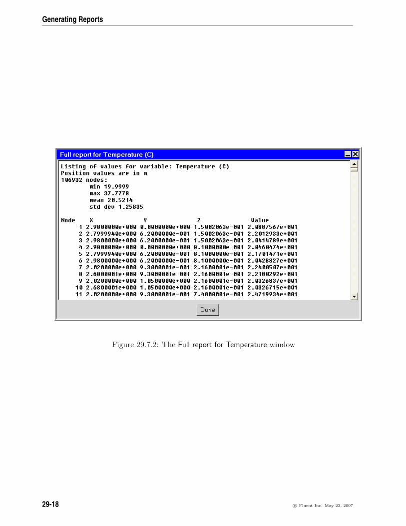
Generating Reports
Figure 29.7.2: The Full report for Temperature window
29-18 c© Fluent Inc. May 22, 2007

29.8 Fan Operating Points Report
29.8 Fan Operating Points Report
You can create a report of the fan operating points for the characteristic curve of fans inyour model. To create a report, select Fan operating points in the Report menu.
Report−→Fan operating points
c© Fluent Inc. May 22, 2007 29-19

Generating Reports
The Message window will report the volume flow rate and pressure rise for the charac-teristic curve of fans in your model. An example is shown below.
Fan "fan.1" vol flow = 3 m3/s, press rise = 300 N/m2
Airpak automatically reports fan operating point data as well as other information at theend of a solution. The report is accessible by selecting Solution overview from the Postmenu. See Section 29.4 for more information about the Solution overview option.
29.9 ADPI Report
You can create a report of the Air Diffusion Performance Index (ADPI) for a specifiedregion in your model. The ADPI is an index for cooling ventilation applications thatmeasures the ventilation performance in the occupied zone.
The ADPI of a region is defined as the percentage of points in the space for which thelocal air velocity is less than 70 ft/min and the effective draft temperature, θED, is in therange −3 < θED < 2.
The effective draft temperature is defined as
θED = (Tair + Troom,avg)− 0.07(vair − 30) (29.9-1)
where
Tair = local air temperature (F)Troom,avg = average room temperature (F)vair = local air velocity (ft/min)
You can use the ADPI specification panel to specify the region of the model on which toreport your results. To open the ADPI specification panel, click on ADPI in the Reportmenu.
Report−→ADPI
To create an ADPI report, use the following procedure:
1. Specify the region on which you want to report. There are two options:
Entire volume indicates that the report will be generated on the entire volumeof your Airpak model.
Region indicates that the report will be generated on a specific region withinyour Airpak model. You will need to specify the bounding coordinates of thedesired region (Min X, Min Y, Min Z, Max X, Max Y, and Max Z).
29-20 c© Fluent Inc. May 22, 2007

29.9 ADPI Report
Figure 29.9.1: The ADPI specification Panel
2. Specify the Number of samples (or points) on which you want to base the ADPIreport. The default value is 1000.
3. Click Accept.
The Message window will report the ADPI value. An example is shown below.
ADPI = 80%
i Note that the ADPI is relevant only for cooling applications.
c© Fluent Inc. May 22, 2007 29-21

Generating Reports
29-22 c© Fluent Inc. May 22, 2007

Chapter 30. Variables for Postprocessing and Reporting
In Airpak, variables are used within the various postprocessing and reporting operationsfor a variety of purposes, such as determining the color spectrum to be applied to acontour plot. This chapter provides definitions of the variables that are contained inthe Variable and Value drop-down lists that appear in the postprocessing and reportingpanels. See Chapter 28 for details on displaying and plotting variables and Chapter 29for details on generating reports.
Information in this chapter is presented in the following sections:
• Section 30.1: General Information about Variables
• Section 30.2: Definitions of Variables
30.1 General Information about Variables
Airpak has two kinds of variables: scalar and vector. Scalar variables consist of a singlevalue at each point in the solution domain, and vector variables consist of three values(one for each coordinate direction) at each point in the domain.
Scalar and vector variables are further divided into two types: primary and derived. Aprimary solution variable is one for which Airpak solves directly when performing thesimulation. The primary variables are pressure, temperature, and the three componentsof velocity. If you are modeling turbulence with the two-equation (standard k-ε) model,the enhanced two-equation model, or the RNG k-ε model, the turbulent kinetic energyand dissipation rate will also be primary solution variables. Derived solution variablesare variables that Airpak computes from the primary variables during postprocessing. Forexample, heat flux is a derived variable computed from the temperature field.
Not all variables, either primary or derived, are available for all simulations. In anisothermal simulation, for example, neither the temperature nor any derived variablebased on temperature (e.g., heat flux) will be available for postprocessing analysis. Forlaminar solutions, or for turbulent solutions that use the zero-equation turbulence model,the turbulent kinetic energy and dissipation will not be available.
c© Fluent Inc. May 22, 2007 30-1

Variables for Postprocessing and Reporting
30.2 Definitions of Variables
30.2.1 Velocity-Related Quantities
Velocity-related quantities that can be reported are as follows:
• UX is the x component of the velocity vector and is available when flow is computed.
• UY is the y component of the velocity vector and is available when flow is computed.
• UZ is the z component of the velocity vector and is available when flow is computed.
• Speed is the magnitude of the velocity vector and is available when flow is computed.
ω = ∇× ~u (30.2-1)
• Mass flow is a derived scalar quantity computed from the velocity field. The flowrate can be computed only on the surface of model objects (typically, a fan, vent,or opening); it cannot be computed for plane cuts or isosurfaces.
• Volume flow is a derived scalar quantity computed from the velocity field. The flowrate can be computed only on the surface of model objects (typically, a fan, vent,or opening); it cannot be computed for plane cuts or isosurfaces.
• Angular deviation is a derived scalar quantity computed from the velocity field. Theangular deviation is computed as
cos θ =u · d|u||d|
(30.2-2)
where u is the local velocity vector, d is a reference direction vector, and θ is theangular deviation. To specify the reference direction vector, click on the Parametersbutton for the Variable list or the Edit button under Params, and enter the X di-rection, Y direction, and Z direction components of the reference direction vector inthe Angular deviation panel (Figure 30.2.1). Click Compute to compute the angulardeviation of the local velocity vector in degrees.
30.2.2 Pressure-Related Quantities
Pressure-related quantities that can be reported are as follows:
• Pressure is the relative static pressure of the fluid and is available when flow iscomputed.
30-2 c© Fluent Inc. May 22, 2007

30.2 Definitions of Variables
Figure 30.2.1: The Angular deviation Panel
30.2.3 Temperature-Related Quantities
Temperature-related quantities that can be reported are as follows:
• Temperature is available when temperature is computed.
• Heat flux is a derived scalar quantity computed from the temperature field. Theheat flux can be computed only on the surface of model objects; it cannot becomputed for plane cuts or isosurfaces. Two types of heat flux can be computedon an object face:
– the heat flux, qd, at a point on a surface (wall) is computed from
qd = −k∇T · ~n (30.2-3)
where k is the conductivity of the material, T is the temperature, and ~n is thenormal to the surface.
– the heat flux, qc, at flow boundaries (e.g., openings, vents, fans) is computedfrom
qc = ρcp(T − Tref)~u · ~n (30.2-4)
where ρ is the density of the fluid, cp is the specific heat, Tref is 298 K, and ~uis the velocity.
• Heat flow is a derived scalar quantity computed from the temperature field. Theheat flow can be computed only on the surface of model objects; it cannot becomputed for plane cuts or isosurfaces. Two types of heat flow can be computedon an object face:
– the heat flow, qd, at a point on a surface (wall) is computed from
qd = −Ak∇T · ~n (30.2-5)
c© Fluent Inc. May 22, 2007 30-3

Variables for Postprocessing and Reporting
where A is the surface area of the face, k is the conductivity of the material,T is the temperature, and ~n is the normal to the surface.
– the heat flow, qc, at flow boundaries (e.g., openings, vents, fans) is computedfrom
qc = Aρcp(T − Tref)~u · ~n (30.2-6)
where A is the surface area of the face, ρ is the density of the fluid, cp is thespecific heat, Tref is 298 K, and ~u is the velocity.
• Heat tr. coeff is a derived scalar quantity computed from the temperature field. Theheat transfer coefficient can be computed only on the surface of model objects; itcannot be computed for plane cuts or isosurfaces.
The heat transfer coefficient is computed as
h =q
T − Tref
(30.2-7)
where q is the heat flux for the surface and Tref is a reference temperature. Tospecify the reference temperature, click on the Parameters button for the Contoursof drop-down list or click the Edit button under Params in the Define summary reportpanel. Specify the temperature next to Ref temp in the Heat tr. coeff parameterspanel (Figure 30.2.2).
Figure 30.2.2: The Heat tr. coeff parameters Panel
30.2.4 Radiation-Related Quantities
Radiation-related quantities that can be reported are as follows:
• Radiative heat flow is a derived scalar quantity. It is available if you are solving yourproblem with radiation effects. It can be computed only on surfaces of objects.
30-4 c© Fluent Inc. May 22, 2007

30.2 Definitions of Variables
30.2.5 Species-Transport-Related Quantities
Species-transport-related quantities that can be reported are as follows:
• species (mole) is the mole fraction of a particular species in the mixture. Forperfect-gas mixtures, the mole fraction is equal to both the pressure fraction andthe volume fraction, so the ppmv (parts per million by volume) for a species is106 times the mole fraction. Airpak displays the mole fraction for species (mole) bydefault. To display the ppmv for the species, you can change the postprocessingunits for concentration to ppmv using the Postprocessing units panel (see Section 5.5for details on changing units for postprocessing). Typical concentration values interms of mass per unit volume can be displayed by creating a user-defined unitfor concentration based on the local mole fraction and reference temperatures andpressures. See Section 5.4.3 for details on creating a user-defined unit.
• species (mass) is the mass fraction of a particular species in the mixture.
30.2.6 Position-Related Quantities
Position-related quantities that can be reported are as follows:
• X, Y, Z are the Cartesian coordinates in the x-axis, y-axis, and z-axis directionsrespectively. They are primary variables in the sense that they are always available.These variables are useful for superimposing lines of constant x, y, or z value onthe model.
30.2.7 Turbulence-Related Quantities
Turbulence-related quantities that can be reported are as follows:
• TKE is the turbulent kinetic energy. It can be reported if the two-equation (stan-dard k-ε) turbulence model, the enhanced two-equation model, or the RNG k-εturbulence model is used.
• Epsilon is the turbulent dissipation rate. It can be reported if the two-equation(standard k-ε) turbulence model, the enhanced two-equation model, or the RNGk-ε turbulence model is used.
• Viscosity ratio is the ratio of the turbulent viscosity to the laminar viscosity. It canbe reported if any of the available turbulence models are used.
c© Fluent Inc. May 22, 2007 30-5

Variables for Postprocessing and Reporting
30.2.8 IAQ and Thermal Comfort Quantities
Indoor air quality (IAQ) and thermal comfort quantities that can be reported are asfollows:
• Mean age of air is the average lifetime of air at a particular location in the roomrelative to the time when it first entered the room. It gives an indication of the air“freshness”.
• Radiation temp (the mean radiant temperature) is defined as the uniform tempera-ture of an imaginary enclosure in which the radiant heat transfer from the humanbody equals the radiant heat transfer in the actual non-uniform enclosure. Themean radiant temperature is calculated using the results of the radiant heat trans-fer calculations in Airpak.
• Relative humidity is the percentage fraction of water vapor present in the air/water-vapor mixture in the room relative to a saturated air/water-vapor mixture at thesame temperature.
• PMV (predicted mean vote) is an index indicating the mean vote concerning thethermal sensation of a large group of people expressed on a seven-point thermalsensation scale:
+3 +2 +1 0 −1 −2 −3hot warm slightly neutral slightly cool cold
warm cool
Airpak uses the ISO 7730 standard [?] to calculate PMV in moderate thermal envi-ronments based on air temperature, air velocity, mean radiant temperature, relativehumidity or partial water-vapor pressure, activity level, and the amount and typeof clothing worn. You can specify the values used by Airpak to compute PMV inthe Comfort level panel as described below.
• PPD (predicted percentage dissatisfied) is an index that indicates the number ofthermally dissatisfied people among a large group of people. Airpak uses the ISO7730 standard [?] to calculate PPD in moderate thermal environments. You canspecify the values used by Airpak to calculate PPD in the Comfort level panel asdescribed below.
You can specify the values used by Airpak to compute PMV and PPD in the Comfortlevel panel (Figure 30.2.3). You can open this panel in two ways:
• Click on the Parameters button for the Variable list or click on the Edit button underParams.
30-6 c© Fluent Inc. May 22, 2007

30.2 Definitions of Variables
Figure 30.2.3: The Comfort level Panel
• Click on Comfort level in the Report menu.
Report−→Comfort level
To compute the comfort level, follow the steps below.
1. Specify the External work being done by the person (usually input as 0).
2. Characterize the type and amount of clothing worn (in clo units, which representthe total thermal resistance of the garments worn). There are two options:
Compute allows you to select any number of clothing items to be worn by theperson from the list of available garments. Airpak recomputes the Clothingvalue each time you select a new item of clothing and displays the total thermalresistance of the clothes selected next to Compute. To deselect all the itemsin the list, click None.
Specify allows you to specify a value for the total thermal resistance of thegarments worn.
c© Fluent Inc. May 22, 2007 30-7

Variables for Postprocessing and Reporting
3. Specify the Metabolic rate. There are two options:
Compute allows you to select an activity from the list of available activities. Youcan select only one activity to set the metabolic rate. Airpak will display themetabolic rate for the selected activity next to Compute.
Specify allows you to specify a value for the metabolic rate.
4. Specify the Relative humidity in the room. There are two options:
Compute instructs Airpak to use the relative humidity values computed duringthe calculation of the solution. These values will be available only if Airpakperformed a species calculation for water vapor.
Specify allows you to specify a global value for the relative humidity.
5. Specify the mean radiant temperature (Rad temperature) in the room. There aretwo options:
Compute instructs Airpak to use the radiation temperature computed during thecalculation of the solution to determine the mean radiant temperature.
Specify allows you to specify a global value for the mean radiant temperature.
6. Specify the Air temperature in the room. There are two options:
Compute instructs Airpak to use the values for the air temperature it computedwhen calculating the solution.
Specify allows you to specify a global value for the air temperature.
7. Specify the Air velocity in the room. There are two options:
Compute instructs Airpak to use the values for the air velocity it computed whencalculating the solution.
Specify allows you to specify a global value for the air velocity.
8. Click the Compute button to compute either PMV or PPD values, depending onyour selection in the Variable or Value list. If you opened the Comfort level panel byclicking Comfort level in the Report menu, Airpak will compute PMV values. Airpakwill display the results in the Message window.
30-8 c© Fluent Inc. May 22, 2007

Chapter 31. Theory
This chapter provides some theoretical background for the models, equations, and solu-tion procedures used by Airpak.
Information is presented in the following sections:
• Section 31.1: Governing Equations
• Section 31.2: Turbulence
• Section 31.3: Buoyancy-Driven Flows and Natural Convection
• Section 31.4: Radiation
• Section 31.5: Optimization
• Section 31.6: Solution Procedures
31.1 Governing Equations
Airpak solves the Navier-Stokes equations for transport of mass, momentum, species, andenergy when it calculates laminar flow with heat transfer. Additional transport equationsare solved when the flow is turbulent (see Section 31.2) or when radiative heat transferis included (see Section 31.4).
31.1.1 The Mass Conservation Equation
The equation for conservation of mass, or continuity equation, can be written as follows:
∂ρ
∂t+∇ · (ρ~v) = 0 (31.1-1)
For an incompressible fluid, this reduces to
∇ · ~v = 0 (31.1-2)
c© Fluent Inc. May 22, 2007 31-1

Theory
31.1.2 Momentum Equations
Transport of momentum in an inertial (non-accelerating) reference frame is describedby [3]
∂
∂t(ρ~v) +∇ · (ρ~v~v) = −∇p+∇ · (τ) + ρ~g + ~F (31.1-3)
where p is the static pressure, τ is the stress tensor (described below), and ρ~g is the
gravitational body force. ~F contains other source terms that may arise from resistances,sources, etc.
The stress tensor τ is given by
τ = µ[(∇~v +∇~vT)− 2
3∇ · ~vI
](31.1-4)
where µ is the molecular viscosity, I is the unit tensor, and the second term on theright-hand side is the effect of volume dilation.
31.1.3 Energy Conservation Equation
The energy equation for a fluid region can be written in terms of sensible enthalpy h(=∫ TTref
cpdT , where Tref is 298.15 K) as
∂
∂t(ρh) +∇ · (ρh~v) = ∇ · [(k + kt)∇T ] + Sh (31.1-5)
where k is the molecular conductivity, kt is the conductivity due to turbulent transport(kt = cpµt/Prt), and the source term Sh includes any volumetric heat sources you havedefined.
In conducting solid regions, Airpak solves a simple conduction equation that includes theheat flux due to conduction and volumetric heat sources within the solid:
∂
∂t(ρh) = ∇ · (k∇T ) + Sh (31.1-6)
where ρ is density, k is conductivity, T is temperature, and Sh is the volumetric heatsource.
Equation 31.1-6 is solved simultaneously with the energy transport equation, Equa-tion 31.1-5, in the flow regions to yield a fully coupled conduction/convection heat transferprediction.
31-2 c© Fluent Inc. May 22, 2007

31.1 Governing Equations
31.1.4 Species Transport Equations
When you choose to solve conservation equations for species, Airpak predicts the localmass fraction of each species, Yi, through the solution of a convection-diffusion equationfor the ith species. This conservation equation takes the following general form:
∂
∂t(ρYi) +∇ · (ρ~vYi) = −∇ · ~Ji + Si (31.1-7)
where Si is the rate of creation by addition from user-defined sources. An equation ofthis form will be solved for N − 1 species where N is the total number of fluid phasespecies present in the system.
Mass Diffusion in Laminar Flows~Ji is the diffusion flux of species i, which arises due to concentration gradients. Airpakuses the dilute approximation, under which the diffusion flux can be written as
~Ji = −ρDi,m∇Yi (31.1-8)
Here Di,m is the diffusion coefficient for species i in the mixture.
Mass Diffusion in Turbulent Flows
In turbulent flows, Airpak computes the mass diffusion in the following form:
~Ji = −(ρDi,m +
µtSct
)∇Yi (31.1-9)
where Sct is the turbulent Schmidt number, µtρDt
(with a default setting of 0.7).
Treatment of Species Transport in the Energy Equation
For many multicomponent mixing flows, the transport of enthalpy due to species diffusion
∇ ·[n∑i=1
(hi) ~Ji
]
can have a significant effect on the enthalpy field and should not be neglected. In par-ticular, when the Lewis number
Lei =k
ρcpDi,m
c© Fluent Inc. May 22, 2007 31-3
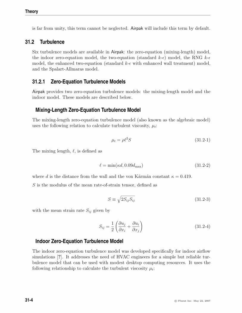
Theory
is far from unity, this term cannot be neglected. Airpak will include this term by default.
31.2 Turbulence
Six turbulence models are available in Airpak: the zero-equation (mixing-length) model,the indoor zero-equation model, the two-equation (standard k-ε) model, the RNG k-εmodel, the enhanced two-equation (standard k-ε with enhanced wall treatment) model,and the Spalart-Allmaras model.
31.2.1 Zero-Equation Turbulence Models
Airpak provides two zero-equation turbulence models: the mixing-length model and theindoor model. These models are described below.
Mixing-Length Zero-Equation Turbulence Model
The mixing-length zero-equation turbulence model (also known as the algebraic model)uses the following relation to calculate turbulent viscosity, µt:
µt = ρ`2S (31.2-1)
The mixing length, `, is defined as
` = min(κd, 0.09dmax) (31.2-2)
where d is the distance from the wall and the von Karman constant κ = 0.419.
S is the modulus of the mean rate-of-strain tensor, defined as
S ≡√
2SijSij (31.2-3)
with the mean strain rate Sij given by
Sij =1
2
(∂uj∂xi
+∂ui∂xj
)(31.2-4)
Indoor Zero-Equation Turbulence Model
The indoor zero-equation turbulence model was developed specifically for indoor airflowsimulations [?]. It addresses the need of HVAC engineers for a simple but reliable tur-bulence model that can be used with modest desktop computing resources. It uses thefollowing relationship to calculate the turbulent viscosity µt:
31-4 c© Fluent Inc. May 22, 2007

31.2 Turbulence
µt = 0.03874ρvL (31.2-5)
where v is the local velocity magnitude, ρ is the fluid density, L is defined as the distancefrom the nearest wall, and 0.03874 is an empirical constant.
Airpak determines the heat transfer at the boundary surfaces by computing a convectiveheat transfer coefficient:
h =µeff
Preff
cp∆xj
(31.2-6)
where cp is the fluid specific heat, Preff is the effective Prandtl number, and ∆xj is thegrid spacing adjacent to the wall. µeff is the effective viscosity, given by
µeff = µ+ µt (31.2-7)
where µ is the viscosity of the fluid.
This model is ideally suited for predicting indoor air flows that consider natural convec-tion, forced convection, mixed convection, and displacement ventilation.
31.2.2 Advanced Turbulence Models
In turbulence models that employ the Boussinesq approach, the central issue is how theeddy viscosity is computed. The model proposed by Spalart and Allmaras [29] solvesa transport equation for a quantity that is a modified form of the turbulent kinematicviscosity.
Both the standard and RNG k-ε models have similar forms, with transport equations fork and ε. The major differences in the models are as follows:
• the method of calculating turbulent viscosity
• the turbulent Prandtl numbers governing the turbulent diffusion of k and ε
• the generation and destruction terms in the ε equation
This section describes the Reynolds-averaging method for calculating turbulent effectsand provides an overview of the issues related to choosing an advanced turbulence modelin Airpak. The transport equations, methods of calculating turbulent viscosity, and modelconstants are presented separately for each model. The features that are essentially com-mon to both models follow, including turbulent production, generation due to buoyancy,and modeling heat transfer.
c© Fluent Inc. May 22, 2007 31-5

Theory
Reynolds (Ensemble) Averaging
The advanced turbulence models in Airpak are based on Reynolds averages of the gov-erning equations. In Reynolds averaging, the solution variables in the instantaneous(exact) Navier-Stokes equations are decomposed into the mean (ensemble-averaged ortime-averaged) and fluctuating components. For the velocity components:
ui = ui + u′i (31.2-8)
where ui and u′i are the mean and instantaneous velocity components (i = 1, 2, 3).
Likewise, for pressure and other scalar quantities:
φ = φ+ φ′ (31.2-9)
where φ denotes a scalar such as pressure or energy.
Substituting expressions of this form for the flow variables into the instantaneous conti-nuity and momentum equations and taking a time (or ensemble) average (and droppingthe overbar on the mean velocity, u) yields the ensemble-averaged momentum equations.They can be written in Cartesian tensor form as:
∂ρ
∂t+
∂
∂xi(ρui) = 0 (31.2-10)
∂
∂t(ρui) +
∂
∂xj(ρuiuj) =
− ∂p
∂xi+
∂
∂xj
[µ
(∂ui∂xj
+∂uj∂xi− 2
3δij∂ul∂xl
)]+
∂
∂xj(−ρu′iu′j) (31.2-11)
Equations 31.2-10 and 31.2-11 are called “Reynolds-averaged” Navier-Stokes (RANS)equations. They have the same general form as the instantaneous Navier-Stokes equa-tions, with the velocities and other solution variables now representing ensemble-averaged(or time-averaged) values. Additional terms now appear that represent the effects ofturbulence. These “Reynolds stresses”, −ρu′iu′j, must be modeled in order to close Equa-tion 31.2-11.
For variable-density flows, Equations 31.2-10 and 31.2-11 can be interpreted as Favre-averaged Navier-Stokes equations [11], with the velocities representing mass-averagedvalues. As such, Equations 31.2-10 and 31.2-11 can be applied to density-varying flows.
31-6 c© Fluent Inc. May 22, 2007

31.2 Turbulence
Boussinesq Approach
The Reynolds-averaged approach to turbulence modeling requires that the Reynoldsstresses in Equation 31.2-11 be appropriately modeled. A common method employs theBoussinesq hypothesis [11] to relate the Reynolds stresses to the mean velocity gradients:
− ρu′iu′j = µt
(∂ui∂xj
+∂uj∂xi
)− 2
3
(ρk + µt
∂ui∂xi
)δij (31.2-12)
The Boussinesq hypothesis is used in the Spalart-Allmaras model and the k-ε models.The advantage of this approach is the relatively low computational cost associated withthe computation of the turbulent viscosity, µt. In the case of the Spalart-Allmaras model,only one additional transport equation (representing turbulent viscosity) is solved. Inthe case of the k-ε models, two additional transport equations (for the turbulence kineticenergy, k, and the turbulence dissipation rate, ε) are solved, and µt is computed as afunction of k and ε. The disadvantage of the Boussinesq hypothesis as presented is thatit assumes µt is an isotropic scalar quantity, which is not strictly true.
Choosing an Advanced Turbulence Model
This section provides an overview of the issues related to the advanced turbulence modelsprovided in Airpak.
The Spalart-Allmaras Model
The Spalart-Allmaras model is a relatively simple one-equation model that solves a mod-eled transport equation for the kinematic eddy (turbulent) viscosity. This embodies arelatively new class of one-equation models in which it is not necessary to calculate alength scale related to the local shear layer thickness. The Spalart-Allmaras model wasdesigned specifically for aerospace applications involving wall-bounded flows and has beenshown to give good results for boundary layers subjected to adverse pressure gradients.It is also gaining popularity for turbomachinery applications.
On a cautionary note, however, the Spalart-Allmaras model is still relatively new, andno claim is made regarding its suitability to all types of complex engineering flows. Forinstance, it cannot be relied on to predict the decay of homogeneous, isotropic turbu-lence. Furthermore, one-equation models are often criticized for their inability to rapidlyaccommodate changes in length scale, such as might be necessary when the flow changesabruptly from a wall-bounded to a free shear flow.
The Standard k-ε Model
The simplest “complete models” of turbulence are two-equation models in which thesolution of two separate transport equations allows the turbulent velocity and lengthscales to be independently determined. The standard k-ε model in Airpak falls within
c© Fluent Inc. May 22, 2007 31-7

Theory
this class of turbulence model and has become the workhorse of practical engineering flowcalculations in the time since it was proposed by Launder and Spalding [19]. Robust-ness, economy, and reasonable accuracy for a wide range of turbulent flows explain itspopularity in industrial flow and heat transfer simulations. It is a semi-empirical model,and the derivation of the model equations relies on phenomenological considerations andempiricism.
As the strengths and weaknesses of the standard k-ε model have become known, improve-ments have been made to the model to improve its performance. One of these variantsis available in Airpak: the RNG k-ε model [32].
The RNG k-ε Model
The RNG k-ε model was derived using a rigorous statistical technique (called renormal-ization group theory). It is similar in form to the standard k-ε model, but includes thefollowing refinements:
• The RNG model has an additional term in its ε equation that significantly improvesthe accuracy for rapidly strained flows.
• The effect of swirl on turbulence is included in the RNG model, enhancing accuracyfor swirling flows.
• The RNG theory provides an analytical formula for turbulent Prandtl numbers,while the standard k-ε model uses user-specified, constant values.
• While the standard k-ε model is a high-Reynolds-number model, the RNG the-ory provides an analytically-derived differential formula for effective viscosity thataccounts for low-Reynolds-number effects.
These features make the RNG k-ε model more accurate and reliable for a wider class offlows than the standard k-ε model.
The Enhanced Two-Equation Model
The k-ε models are primarily valid for turbulent core flows (i.e., the flow in the regionssomewhat far from walls). Consideration therefore needs to be given as to how to makethese models suitable for wall-bounded flows.
Turbulent flows are significantly affected by the presence of walls. Obviously, the meanvelocity field is affected through the no-slip condition that has to be satisfied at the wall.However, the turbulence is also changed by the presence of the wall in non-trivial ways.Very close to the wall, viscous damping reduces the tangential velocity fluctuations, whilekinematic blocking reduces the normal fluctuations. Toward the outer part of the near-wall region, however, the turbulence is rapidly augmented by the production of turbulencekinetic energy due to the large gradients in mean velocity.
31-8 c© Fluent Inc. May 22, 2007

31.2 Turbulence
The near-wall modeling significantly impacts the fidelity of numerical solutions, inasmuchas walls are the main source of mean vorticity and turbulence. It is in the near-wall regionwhere the solution variables have large gradients and where the momentum and otherscalar transports are the greatest. Therefore, accurate representation of the flow in thenear-wall region determines successful predictions of wall-bounded turbulent flows.
Numerous experiments have shown that the near-wall region can be largely subdividedinto three layers. In the innermost layer, called the “viscous sublayer”, the flow is almostlaminar, and the (molecular) viscosity plays a dominant role in momentum and heator mass transfer. In the outer layer, called the fully-turbulent layer, turbulence playsa major role. Finally, there is an interim region between the viscous sublayer and thefully turbulent layer where the effects of molecular viscosity and turbulence are equallyimportant.
To more accurately resolve the flow near the wall, the enhanced two-equation modelcombines the standard k-ε model with enhanced wall treatment.
Enhanced Wall Treatment
Enhanced wall treatment is a near-wall modeling method that combines a two-layer modelwith enhanced wall functions [4, 12, 15, 16, 30, 31].
In the two-layer model, the viscosity-affected near-wall region is completely resolvedall the way to the viscous sublayer. The two-layer approach is an integral part of theenhanced wall treatment and is used to specify both ε and the turbulent viscosity in thenear-wall cells. In this approach, the whole domain is subdivided into a viscosity-affectedregion and a fully-turbulent region. The demarcation of the two regions is determinedby a wall-distance-based, turbulent Reynolds number.
If the near-wall mesh is fine enough to be able to resolve the laminar sublayer (typicallyy+ ≈ 1), then the enhanced wall treatment will be identical to the traditional two-layerzonal model. However, the restriction that the near-wall mesh must be sufficiently fineeverywhere might impose too large a computational requirement. Ideally, then, onewould like to have a near-wall formulation that can be used with coarse meshes (usuallyreferred to as wall-function meshes) as well as fine meshes (low-Reynolds-number meshes).In addition, excessive error should not be incurred for intermediate meshes that are toofine for the near-wall cell centroid to lie in the fully turbulent region, but also too coarseto properly resolve the sublayer.
To achieve the goal of having a near-wall modeling approach that will possess the accuracyof the standard two-layer approach for fine near-wall meshes and will not significantlyreduce accuracy for wall-function meshes, Airpak combines the two-layer model withenhanced wall functions to result in the enhanced wall treatment.
c© Fluent Inc. May 22, 2007 31-9
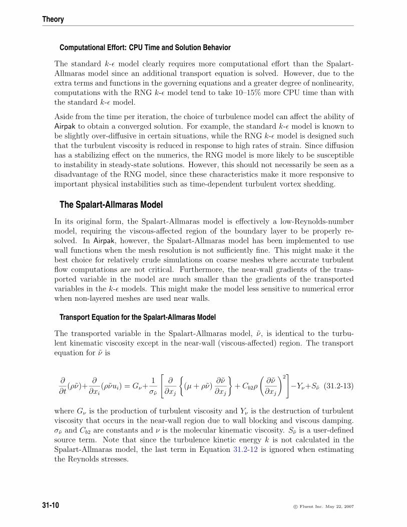
Theory
Computational Effort: CPU Time and Solution Behavior
The standard k-ε model clearly requires more computational effort than the Spalart-Allmaras model since an additional transport equation is solved. However, due to theextra terms and functions in the governing equations and a greater degree of nonlinearity,computations with the RNG k-ε model tend to take 10–15% more CPU time than withthe standard k-ε model.
Aside from the time per iteration, the choice of turbulence model can affect the ability ofAirpak to obtain a converged solution. For example, the standard k-ε model is known tobe slightly over-diffusive in certain situations, while the RNG k-ε model is designed suchthat the turbulent viscosity is reduced in response to high rates of strain. Since diffusionhas a stabilizing effect on the numerics, the RNG model is more likely to be susceptibleto instability in steady-state solutions. However, this should not necessarily be seen as adisadvantage of the RNG model, since these characteristics make it more responsive toimportant physical instabilities such as time-dependent turbulent vortex shedding.
The Spalart-Allmaras Model
In its original form, the Spalart-Allmaras model is effectively a low-Reynolds-numbermodel, requiring the viscous-affected region of the boundary layer to be properly re-solved. In Airpak, however, the Spalart-Allmaras model has been implemented to usewall functions when the mesh resolution is not sufficiently fine. This might make it thebest choice for relatively crude simulations on coarse meshes where accurate turbulentflow computations are not critical. Furthermore, the near-wall gradients of the trans-ported variable in the model are much smaller than the gradients of the transportedvariables in the k-ε models. This might make the model less sensitive to numerical errorwhen non-layered meshes are used near walls.
Transport Equation for the Spalart-Allmaras Model
The transported variable in the Spalart-Allmaras model, ν, is identical to the turbu-lent kinematic viscosity except in the near-wall (viscous-affected) region. The transportequation for ν is
∂
∂t(ρν)+
∂
∂xi(ρνui) = Gν+
1
σν
∂
∂xj
(µ+ ρν)
∂ν
∂xj
+ Cb2ρ
(∂ν
∂xj
)2−Yν+Sν (31.2-13)
where Gν is the production of turbulent viscosity and Yν is the destruction of turbulentviscosity that occurs in the near-wall region due to wall blocking and viscous damping.σν and Cb2 are constants and ν is the molecular kinematic viscosity. Sν is a user-definedsource term. Note that since the turbulence kinetic energy k is not calculated in theSpalart-Allmaras model, the last term in Equation 31.2-12 is ignored when estimatingthe Reynolds stresses.
31-10 c© Fluent Inc. May 22, 2007

31.2 Turbulence
Modeling the Turbulent Viscosity
The turbulent viscosity, µt, is computed from
µt = ρνfv1 (31.2-14)
where the viscous damping function, fv1, is given by
fv1 =χ3
χ3 + C3v1
(31.2-15)
and
χ ≡ ν
ν(31.2-16)
Modeling the Turbulent Production
The production term, Gν , is modeled as
Gν = Cb1ρSν (31.2-17)
where
S ≡ S +ν
κ2d2fv2 (31.2-18)
and
fv2 = 1− χ
1 + χfv1
(31.2-19)
Cb1 and κ are constants, d is the distance from the wall, and S is a scalar measure of thedeformation tensor. By default in Airpak, as in the original model proposed by Spalartand Allmaras, S is based on the magnitude of the vorticity:
S ≡√
2ΩijΩij (31.2-20)
where Ωij is the mean rate-of-rotation tensor and is defined by
Ωij =1
2
(∂ui∂xj− ∂uj∂xi
)(31.2-21)
c© Fluent Inc. May 22, 2007 31-11

Theory
The justification for the default expression for S is that, for the wall-bounded flows thatwere of most interest when the model was formulated, turbulence is found only wherevorticity is generated near walls. However, it has since been acknowledged that oneshould also take into account the effect of mean strain on the turbulence production, anda modification to the model has been proposed [9] and incorporated into Airpak.
This modification combines measures of both rotation and strain tensors in the definitionof S:
S ≡ |Ωij|+ Cprod min (0, |Sij| − |Ωij|) (31.2-22)
where
Cprod = 2.0, |Ωij| ≡√
2ΩijΩij, |Sij| ≡√
2SijSij
with the mean strain rate, Sij, defined as
Sij =1
2
(∂uj∂xi
+∂ui∂xj
)(31.2-23)
Including both the rotation and strain tensors reduces the production of eddy viscosityand consequently reduces the eddy viscosity itself in regions where the measure of vortic-ity exceeds that of strain rate. One such example can be found in vortical flows, i.e., flownear the core of a vortex subjected to a pure rotation where turbulence is known to besuppressed. Including both the rotation and strain tensors more correctly accounts forthe effects of rotation on turbulence. The default option (including the rotation tensoronly) tends to overpredict the production of eddy viscosity and hence overpredicts theeddy viscosity itself in certain circumstances.
31-12 c© Fluent Inc. May 22, 2007

31.2 Turbulence
Modeling the Turbulent Destruction
The destruction term is modeled as
Yν = Cw1ρfw
(ν
d
)2
(31.2-24)
where
fw = g
[1 + C6
w3
g6 + C6w3
]1/6
(31.2-25)
g = r + Cw2
(r6 − r
)(31.2-26)
r ≡ ν
Sκ2d2(31.2-27)
Cw1, Cw2, and Cw3 are constants, and S is given by Equation 31.2-18. Note that themodification described above to include the effects of mean strain on S will also affectthe value of S used to compute r.
Model Constants
The model constants Cb1, Cb2, σν , Cv1, Cw1, Cw2, Cw3, and κ have the following defaultvalues [29]:
Cb1 = 0.1355, Cb2 = 0.622, σν =2
3, Cv1 = 7.1
Cw1 =Cb1κ2
+(1 + Cb2)
σν, Cw2 = 0.3, Cw3 = 2.0, κ = 0.4187
Wall Boundary Conditions
At walls, the modified turbulent kinematic viscosity, ν, is set to zero.
When the mesh is fine enough to resolve the laminar sublayer, the wall shear stress isobtained from the laminar stress-strain relationship:
u
uτ=ρuτy
µ(31.2-28)
c© Fluent Inc. May 22, 2007 31-13

Theory
If the mesh is too coarse to resolve the laminar sublayer, it is assumed that the centroidof the wall-adjacent cell falls within the logarithmic region of the boundary layer, andthe law-of-the-wall is employed:
u
uτ=
1
κlnE
(ρuτy
µ
)(31.2-29)
where u is the velocity parallel to the wall, uτ is the shear velocity, y is the distance fromthe wall, κ is the von Karman constant (0.4187), and E = 9.793.
Convective Heat and Mass Transfer Modeling
In Airpak, turbulent heat transport is modeled using the concept of Reynolds’ analogyto turbulent momentum transfer. The “modeled” energy equation is thus given by thefollowing:
∂
∂t(ρE) +
∂
∂xi[ui(ρE + p)] =
∂
∂xj
[(k +
cpµtPrt
)∂T
∂xj+ ui(τij)eff
]+ Sh (31.2-30)
where k, in this case, is the thermal conductivity, E is the total energy, and (τij)eff is thedeviatoric stress tensor, defined as
(τij)eff = µeff
(∂uj∂xi
+∂ui∂xj
)− 2
3µeff
∂ui∂xi
δij
The term involving (τij)eff represents the viscous heating. The default value of the turbu-lent Prandtl number is 0.85. Turbulent mass transfer is treated similarly, with a defaultturbulent Schmidt number of 0.7.
Wall boundary conditions for scalar transport are handled analogously to momentum,using the appropriate “law-of-the-wall”.
Two-Equation (Standard k-ε) Turbulence Model
The two-equation turbulence model (also known as the standard k-ε model) is morecomplex than the zero-equation model. The standard k-ε model [19] is a semi-empiricalmodel based on model transport equations for the turbulent kinetic energy (k) and itsdissipation rate (ε). The model transport equation for k is derived from the exact equa-tion, while the model transport equation for ε is obtained using physical reasoning andbears little resemblance to its mathematically exact counterpart.
In the derivation of the standard k-ε model, it is assumed that the flow is fully turbulent,and the effects of molecular viscosity are negligible. The standard k-ε model is thereforevalid only for fully turbulent flows.
31-14 c© Fluent Inc. May 22, 2007

31.2 Turbulence
Transport Equations for the Standard k-ε Model
The turbulent kinetic energy, k, and its rate of dissipation, ε, are obtained from thefollowing transport equations:
∂
∂t(ρk) +
∂
∂xi(ρkui) =
∂
∂xi
[(µ+
µtσk
)∂k
∂xi
]+Gk +Gb − ρε (31.2-31)
and
∂
∂t(ρε) +
∂
∂xi(ρεui) =
∂
∂xi
[(µ+
µtσε
)∂ε
∂xi
]+ C1ε
ε
k(Gk + C3εGb)− C2ερ
ε2
k(31.2-32)
In these equations, Gk represents the generation of turbulent kinetic energy due to themean velocity gradients, calculated as described later in this section. Gb is the generationof turbulent kinetic energy due to buoyancy, calculated as described later in this section.C1ε, C2ε, and C3ε are constants. σk and σε are the turbulent Prandtl numbers for k andε, respectively.
Modeling the Turbulent Viscosity
The “eddy” or turbulent viscosity, µt, is computed by combining k and ε as follows:
µt = ρCµk2
ε(31.2-33)
where Cµ is a constant.
Model Constants
The model constants C1ε, C2ε, Cµ, σk, and σε have the following default values [19]:
C1ε = 1.44, C2ε = 1.92, Cµ = 0.09, σk = 1.0, σε = 1.3
These default values have been determined from experiments with air and water for funda-mental turbulent shear flows including homogeneous shear flows and decaying isotropicgrid turbulence. They have been found to work fairly well for a wide range of wall-bounded and free shear flows.
c© Fluent Inc. May 22, 2007 31-15

Theory
The RNG k-ε Model
The RNG-based k-ε turbulence model is derived from the instantaneous Navier-Stokesequations, using a mathematical technique called “renormalization group” (RNG) meth-ods. The analytical derivation results in a model with constants different from those inthe standard k-ε model, and additional terms and functions in the transport equationsfor k and ε. A more comprehensive description of RNG theory and its application toturbulence can be found in [6].
Transport Equations for the RNG k-ε Model
The RNG k-ε model has a similar form to the standard k-ε model:
∂
∂t(ρk) +
∂
∂xi(ρkui) =
∂
∂xi
(αkµeff
∂k
∂xi
)+Gk +Gb − ρε (31.2-34)
and
∂
∂t(ρε) +
∂
∂xi(ρεui) =
∂
∂xi
(αεµeff
∂ε
∂xi
)+ C1ε
ε
k(Gk + C3εGb)− C2ερ
ε2
k−Rε (31.2-35)
In these equations, Gk represents the generation of turbulent kinetic energy due to themean velocity gradients, calculated as described later in this section. Gb is the gener-ation of turbulent kinetic energy due to buoyancy, calculated as described later in thissection. The quantities αk and αε are the inverse effective Prandtl numbers for k and ε,respectively.
Modeling the Effective Viscosity
The scale elimination procedure in RNG theory results in a differential equation forturbulent viscosity:
d
(ρ2k√εµ
)= 1.72
ν√ν3 − 1 + Cν
dν (31.2-36)
where
ν = µeff/µ
Cν ≈ 100
Equation 31.2-36 is integrated to obtain an accurate description of how the effectiveturbulent transport varies with the effective Reynolds number (or eddy scale), allowingthe model to better handle low-Reynolds-number and near-wall flows.
31-16 c© Fluent Inc. May 22, 2007

31.2 Turbulence
In the high-Reynolds-number limit, Equation 31.2-36 gives
µt = ρCµk2
ε(31.2-37)
with Cµ = 0.0845, derived using RNG theory. It is interesting to note that this valueof Cµ is very close to the empirically-determined value of 0.09 used in the standard k-εmodel.
In Airpak, the effective viscosity is computed using the high-Reynolds-number form inEquation 31.2-37.
Calculating the Inverse Effective Prandtl Numbers
The inverse effective Prandtl numbers αk and αε are computed using the following formuladerived analytically by the RNG theory:
∣∣∣∣ α− 1.3929
α0 − 1.3929
∣∣∣∣0.6321 ∣∣∣∣ α + 2.3929
α0 + 2.3929
∣∣∣∣0.3679
=µmol
µeff
(31.2-38)
where α0 = 1.0. In the high-Reynolds-number limit (µmol/µeff 1), αk = αε ≈ 1.393.
The Rε Term in the ε Equation
The main difference between the RNG and standard k-ε models lies in the additionalterm in the ε equation given by
Rε =Cµρη
3(1− η/η0)
1 + βη3
ε2
k(31.2-39)
where η ≡ Sk/ε, η0 = 4.38, β = 0.012.
The effects of this term in the RNG ε equation can be seen more clearly by rearrangingEquation 31.2-35. Using Equation 31.2-39, the last two terms in Equation 31.2-35 canbe merged, and the resulting ε equation can be rewritten as
∂
∂t(ρε) +
∂
∂xi(ρεui) =
∂
∂xj
(αεµeff
∂ε
∂xj
)+ C1ε
ε
k(Gk + C3εGb)− C∗2ερ
ε2
k(31.2-40)
where C∗2ε is given by
C∗2ε ≡ C2ε +Cµρη
3(1− η/η0)
1 + βη3(31.2-41)
c© Fluent Inc. May 22, 2007 31-17

Theory
In regions where η < η0, the R term makes a positive contribution, and C∗2ε becomeslarger than C2ε. In the logarithmic layer, for instance, it can be shown that η ≈ 3.0,giving C∗2ε ≈ 2.0, which is close in magnitude to the value of C2ε in the standard k-εmodel (1.92). As a result, for weakly to moderately strained flows, the RNG model tendsto give results largely comparable to the standard k-ε model.
In regions of large strain rate (η > η0), however, the R term makes a negative contribu-tion, making the value of C∗2ε less than C2ε. In comparison with the standard k-ε model,the smaller destruction of ε augments ε, reducing k and eventually the effective viscosity.As a result, in rapidly strained flows, the RNG model yields a lower turbulent viscositythan the standard k-ε model.
Thus, the RNG model is more responsive to the effects of rapid strain and streamlinecurvature than the standard k-ε model, which explains the superior performance of theRNG model for certain classes of flows.
Model Constants
The model constants C1ε and C2ε in Equation 31.2-35 have values derived analyticallyby the RNG theory. These values, used by default in Airpak, are
C1ε = 1.42, C2ε = 1.68
Modeling Turbulent Production in the k-ε Models
From the exact equation for the transport of k, the term Gk, representing the productionof turbulent kinetic energy, can be defined as
Gk = −ρu′iu′j∂uj∂xi
(31.2-42)
To evaluate Gk in a manner consistent with the Boussinesq hypothesis,
Gk = µtS2 (31.2-43)
where S is the modulus of the mean rate-of-strain tensor, defined as
S ≡√
2SijSij (31.2-44)
with the mean strain rate Sij given by
Sij =1
2
(∂uj∂xi
+∂ui∂xj
)(31.2-45)
31-18 c© Fluent Inc. May 22, 2007

31.2 Turbulence
Effects of Buoyancy on Turbulence in the k-ε Models
When a non-zero gravity field and temperature gradient are present simultaneously, thek-ε models in Airpak account for the generation of k due to buoyancy (Gb in Equa-tions 31.2-31 and 31.2-34), and the corresponding contribution to the production of ε inEquations 31.2-32 and 31.2-35.
The generation of turbulence due to buoyancy is given by
Gb = βgiµtPrt
∂T
∂xi(31.2-46)
where Prt is the turbulent Prandtl number for energy. For the standard k-ε model, thedefault value of Prt is 0.85. In the case of the RNG k-ε model, Prt = 1/α, where αis given by Equation 31.2-38, but with α0 = 1/Pr = k/µcp. The coefficient of thermalexpansion, β, is defined as
β = −1
ρ
(∂ρ
∂T
)p
(31.2-47)
It can be seen from the transport equation for k (Equation 31.2-31 or 31.2-34) thatturbulent kinetic energy tends to be augmented (Gb > 0) in unstable stratification. Forstable stratification, buoyancy tends to suppress the turbulence (Gb < 0). In Airpak, theeffects of buoyancy on the generation of k are always included when you have both anon-zero gravity field and a non-zero temperature (or density) gradient.
While the buoyancy effects on the generation of k are relatively well understood, theeffect on ε is less clear. In Airpak, by default, the buoyancy effects on ε are neglectedsimply by setting Gb to zero in the transport equation for ε (Equation 31.2-32 or 31.2-35).
The degree to which ε is affected by the buoyancy is determined by the constant C3ε.In Airpak, C3ε is not specified, but is instead calculated according to the following rela-tion [10]:
C3ε = tanh∣∣∣∣vu∣∣∣∣ (31.2-48)
where v is the component of the flow velocity parallel to the gravitational vector andu is the component of the flow velocity perpendicular to the gravitational vector. Inthis way, C3ε will become 1 for buoyant shear layers for which the main flow direction isaligned with the direction of gravity. For buoyant shear layers that are perpendicular tothe gravitational vector, C3ε will become zero.
c© Fluent Inc. May 22, 2007 31-19

Theory
Convective Heat Transfer Modeling in the k-ε Models
In Airpak, turbulent heat transport is modeled using the concept of Reynolds’ analogyto turbulent momentum transfer. The “modeled” energy equation is thus given by thefollowing:
∂
∂t(ρE) +
∂
∂xi[ui(ρE + p)] =
∂
∂xi
(keff
∂T
∂xi
)+ Sh (31.2-49)
where E is the total energy and keff is the effective conductivity.
For the standard k-ε model, keff is given by
keff = k +cpµtPrt
with the default value of the turbulent Prandtl number set to 0.85.
For the RNG k-ε model, the effective thermal conductivity is
keff = αcpµeff
where α is calculated from Equation 31.2-38, but with α0 = 1/Pr = k/µcp.
The fact that α varies with µmol/µeff , as in Equation 31.2-38, is an advantage of theRNG k-ε model. It is consistent with experimental evidence indicating that the tur-bulent Prandtl number varies with the molecular Prandtl number and turbulence [18].Equation 31.2-38 works well across a very broad range of molecular Prandtl numbers,from liquid metals (Pr ≈ 10−2) to paraffin oils (Pr ≈ 103), which allows heat transferto be calculated in low-Reynolds-number regions. Equation 31.2-38 smoothly predictsthe variation of effective Prandtl number from the molecular value (α = 1/Pr) in theviscosity-dominated region to the fully turbulent value (α = 1.393) in the fully turbulentregions of the flow.
31-20 c© Fluent Inc. May 22, 2007

31.3 Buoyancy-Driven Flows and Natural Convection
31.3 Buoyancy-Driven Flows and Natural Convection
The importance of buoyancy forces in a mixed convection flow can be measured by theratio of the Grashof and Reynolds numbers:
Gr
Re2 =gβ∆TL
v2(31.3-1)
When this number approaches or exceeds unity, you should expect strong buoyancycontributions to the flow. Conversely, if it is very small, buoyancy forces may be ignoredin your simulation. In pure natural convection, the strength of the buoyancy-inducedflow is measured by the Rayleigh number:
Ra =gβ∆TL3ρ
µα(31.3-2)
where β is the thermal expansion coefficient:
β = −1
ρ
(∂ρ
∂T
)p
(31.3-3)
and α is the thermal diffusivity:
α =k
ρcp(31.3-4)
Rayleigh numbers less than 108 indicate a buoyancy-induced laminar flow, with transitionto turbulence occurring over the range of 108 < Ra < 1010.
Airpak uses either the Boussinesq model or the ideal gas law in the calculation of natural-convection flows, as described below.
31.3.1 The Boussinesq Model
By default, Airpak uses the Boussinesq model for natural-convection flows. This modeltreats density as a constant value in all solved equations, except for the buoyancy termin the momentum equation:
(ρ− ρ0)g ≈ −ρ0β(T − T0)g (31.3-5)
where ρ0 is the (constant) density of the flow, T0 is the operating temperature, and β isthe thermal expansion coefficient. Equation 31.3-5 is obtained by using the Boussinesq
c© Fluent Inc. May 22, 2007 31-21
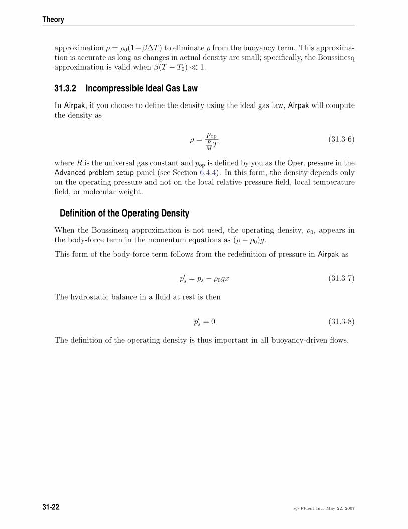
Theory
approximation ρ = ρ0(1−β∆T ) to eliminate ρ from the buoyancy term. This approxima-tion is accurate as long as changes in actual density are small; specifically, the Boussinesqapproximation is valid when β(T − T0) 1.
31.3.2 Incompressible Ideal Gas Law
In Airpak, if you choose to define the density using the ideal gas law, Airpak will computethe density as
ρ =pop
RMT
(31.3-6)
where R is the universal gas constant and pop is defined by you as the Oper. pressure in theAdvanced problem setup panel (see Section 6.4.4). In this form, the density depends onlyon the operating pressure and not on the local relative pressure field, local temperaturefield, or molecular weight.
Definition of the Operating Density
When the Boussinesq approximation is not used, the operating density, ρ0, appears inthe body-force term in the momentum equations as (ρ− ρ0)g.
This form of the body-force term follows from the redefinition of pressure in Airpak as
p′s = ps − ρ0gx (31.3-7)
The hydrostatic balance in a fluid at rest is then
p′s = 0 (31.3-8)
The definition of the operating density is thus important in all buoyancy-driven flows.
31-22 c© Fluent Inc. May 22, 2007

31.4 Radiation
31.4 Radiation
31.4.1 Overview
The terms radiative heat transfer and thermal radiation are commonly used to describeheat transfer caused by electromagnetic (EM) waves. All materials continually emit andabsorb EM waves, or photons. The strength and wavelength of emission depends onthe temperature of the emitting material. At absolute zero K, no radiation is emittedfrom a surface. For heat transfer applications, wavelengths in the infrared spectrum aregenerally of greatest importance and are, therefore, the only ones considered in Airpak.
While both conduction and convection (the other basic modes of heat transfer) require amedium for transmission, radiation does not. Therefore, thermal radiation can traverse along distance without interacting with a medium. Also, for most applications, conductiveand convective heat transfer rates are linearly proportional to temperature differences.Radiative heat transfer rates, on the other hand, are (for the most part) proportional todifferences in temperature raised to the fourth power.
31.4.2 Gray-Diffuse Radiation
Airpak’s radiation models assume the surfaces to be gray and diffuse. Emissivity andabsorptivity of a gray surface are independent of the wavelength. Also, by Kirchhoff’slaw [20], the emissivity equals the absorptivity (ε = α). For a diffuse surface, the reflec-tivity is independent of the outgoing (or incoming) directions.
As stated earlier, for applications of interest, the exchange of radiative energy betweensurfaces is virtually unaffected by the medium that separates them. Thus, accordingto the gray-body model, if a certain amount of radiation (E) is incident on a surface,a fraction (ρE) is reflected, a fraction (αE) is absorbed, and a fraction (τE) is trans-mitted. Since for most indoor applications the surfaces in question are opaque to ther-mal radiation (in the infrared spectrum), the surfaces can be considered opaque. Thetransmissivity, therefore, can be neglected. It follows, from conservation of energy, thatα + ρ = 1, since α = ε (emissivity), and ρ = 1− ε.
31.4.3 Radiative Transfer Equation
The radiative transfer equation (RTE) for an absorbing, emitting, and scattering mediumat position ~r in the direction ~s is
dI(~r, ~s)
ds+ (a+ σs)I(~r, ~s) = an2σT
4
π+σs4π
∫ 4π
0I(~r, ~s ′) Φ(~s · ~s ′) dΩ′ (31.4-1)
c© Fluent Inc. May 22, 2007 31-23

Theory
where ~r = position vector~s = direction vector~s ′ = scattering direction vectors = path lengtha = absorption coefficientn = refractive indexσs = scattering coefficientσ = Stefan-Boltzmann constant (5.672 × 10⁻⁸ W/m2-K4)I = radiation intensity, which depends on position (~r)
and direction (~s)T = local temperatureΦ = phase functionΩ′ = solid angle
(a + σs)s is the optical thickness or opacity of the medium. The refractive index n isimportant when considering radiation in semi-transparent media. Figure 31.4.1 illustratesthe process of radiation heat transfer.
ds
Incomingradiation (I)
Outgoing radiation I + (dI/ds)ds
Absorption andscattering loss: I (a+ σs) ds
Gas emission:(aσT / π) ds4
Scatteringaddition
Figure 31.4.1: Radiation Heat Transfer
31.4.4 The Surface-to-Surface Radiation Model
The default radiation model used in Airpak is the surface-to-surface radiation model. Theenergy flux leaving a given surface is composed of directly emitted and reflected energy.The reflected energy flux is dependent on the incident energy flux from the surroundings,which then can be expressed in terms of the energy flux leaving all other surfaces. Theenergy reflected from surface k is
31-24 c© Fluent Inc. May 22, 2007

31.4 Radiation
qout,k = εkσT4k + ρkqin,k (31.4-2)
where qout,k is the energy flux leaving the surface, εk is the emissivity, σ is the Boltzmannconstant, and qin,k is the energy flux incident on the surface from the surroundings.
The amount of incident energy upon a surface from another surface is a direct functionof the surface-to-surface “view factor,” Fjk. The view factor Fjk is the fraction of energyleaving surface k that is incident on surface j. The incident energy flux qin,k can beexpressed in terms of the energy flux leaving all other surfaces as
Akqin,k =N∑j=1
Ajqout,jFjk (31.4-3)
where Ak is the area of surface k and Fjk is the view factor between surface k and surfacej. For N surfaces, using the view factor reciprocity relationship gives
AjFjk = AkFkj for j = 1, 2, 3, . . . N (31.4-4)
so that
qin,k =N∑j=1
Fkjqout,j (31.4-5)
Therefore,
qout,k = εkσT4k + ρk
N∑j=1
Fkjqout,j (31.4-6)
which can be written as
Jk = Ek + ρkN∑j=1
FkjJj (31.4-7)
where Jk represents the energy that is given off (or radiosity) of surface k and Ek repre-sents the emissive power of surface k. This represents N equations, which can be recastinto matrix form as
KJ = E (31.4-8)
where K is an N × N matrix, J is the radiosity vector, and E is the emissive powervector.
c© Fluent Inc. May 22, 2007 31-25

Theory
Equation 31.4-8 is referred to as the radiosity matrix equation. The view factor betweentwo finite surfaces i and j is given by
Fij =1
Ai
∫Ai
∫Aj
cos θi cos θjπr2
δijdAidAj (31.4-9)
where δij is determined by the visibility of dAj to dAi. δij = 1 if dAj is visible to dAiand 0 otherwise.
31.4.5 The Discrete Ordinates (DO) Radiation Model
The discrete ordinates (DO) radiation model solves the radiative transfer equation (RTE)for a finite number of discrete solid angles, each associated with a vector direction ~s fixedin the global Cartesian system (x, y, z). The fineness of the angular discretization is setby default parameters that depend on the type of problem you are solving. The DOmodel transforms Equation 31.4-1 into a transport equation for radiation intensity in thespatial coordinates (x, y, z). The DO model solves for as many transport equations asthere are directions ~s. The solution method is identical to that used for the fluid flowand energy equations.
The implementation in Airpak uses a conservative variant of the discrete ordinates modelcalled the finite-volume scheme [7, 23], and its extension to unstructured meshes [21].
The DO Equations
The DO model considers the radiative transfer equation (RTE) in the direction ~s as afield equation. Thus, Equation 31.4-1 is written as
∇ · (I(~r, ~s)~s) + (a+ σs)I(~r, ~s) = an2σT4
π+σs4π
∫ 4π
0I(~r, ~s ′) Φ(~s · ~s ′) dΩ′ (31.4-10)
Angular Discretization and Pixelation
Each octant of the angular space 4π at any spatial location is discretized into Nθ × Nφ
solid angles of extent ωi, called control angles. The angles θ and φ are the polar andazimuthal angles respectively, and are measured with respect to the global Cartesiansystem (x, y, z) as shown in Figure 31.4.2. The θ and φ extents of the control angle, ∆θand ∆φ, are constant.
When Cartesian meshes are used, it is possible to align the global angular discretizationwith the control volume face, as shown in Figure 31.4.3. For generalized unstructuredmeshes, however, control volume faces do not in general align with the global angulardiscretization, as shown in Figure 31.4.4, leading to the problem of control angle over-hang [21].
31-26 c© Fluent Inc. May 22, 2007

31.4 Radiation
Figure 31.4.2: Angular Coordinate System
Figure 31.4.3: Face with No Control Angle Overhang
Figure 31.4.4: Face with Control Angle Overhang
c© Fluent Inc. May 22, 2007 31-27

Theory
Essentially, control angles can straddle the control volume faces, so that they are partiallyincoming and partially outgoing to the face. Figure 31.4.5 shows a 3D example of a facewith control angle overhang.
Figure 31.4.5: Face with Control Angle Overhang (3D)
The control volume face cuts the sphere representing the angular space at an arbitraryangle. The line of intersection is a great circle. Control angle overhang may also occuras a result of reflection and refraction. It is important in these cases to correctly accountfor the overhanging fraction. This is done through the use of pixelation [21].
31-28 c© Fluent Inc. May 22, 2007

31.4 Radiation
Each overhanging control angle is divided into Nθp×Nφp pixels, as shown in Figure 31.4.6.The energy contained in each pixel is then treated as incoming or outgoing to the face.The influence of overhang can thus be accounted for within the pixel resolution. For prob-lems involving gray-diffuse radiation, the default pixelation of 1× 1 is usually sufficient.For problems involving symmetry boundaries, a pixelation of 3× 3 is used.
Figure 31.4.6: Pixelation of Control Angle
Boundary Condition Treatment at Gray-Diffuse Walls
For gray radiation, the incident radiation heat flux, qin, at the wall is
qin =∫~s·~n>0
Iin~s · ~ndΩ (31.4-11)
The net radiative flux leaving the surface is given by
qout = (1− εw)qin + n2εwσT4w (31.4-12)
where n is the refractive index of the medium next to the wall. The boundary intensityfor all outgoing directions ~s at the wall is given by
I0 = qout/π (31.4-13)
c© Fluent Inc. May 22, 2007 31-29

Theory
Boundary Condition Treatment at Symmetry Boundaries
At symmetry boundaries, the direction of the reflected ray ~sr corresponding to the in-coming direction ~s is given by
~sr = ~s− 2 (~s · ~n)~n (31.4-14)
Furthermore,
Iw(~sr) = Iw(~s) (31.4-15)
Boundary Condition Treatment at Flow Inlets and Exits
The net radiation heat flux at flow inlets and outlets is computed in the same manneras at walls, as described above. Airpak assumes that the emissivity of all flow inlets andoutlets is 1.0 (black body absorption).
31.5 Optimization
Airpak uses the Dynamic-Q optimization method to solve design optimization problems.The Dynamic-Q method is an efficient constrained-optimization method consisting ofapplying a dynamic-trajectory-optimization algorithm to successive quadratic approxi-mations of the actual optimization problem.
Due to its efficiency with respect to the number of function evaluations required for con-vergence, the Dynamic-Q method is primarily intended for optimization problems wherefunction evaluations are computationally expensive. Such problems occur frequently inengineering applications where time consuming numerical simulations may be used forfunction evaluations. Among others, these numerical analysis may take the form of acomputational fluid dynamics (CFD) simulation, a structural analysis by means of thefinite element method (FEM), or a dynamic simulation of a multibody system. Becausethese simulations are usually computationally expensive to perform, and because the rel-evant functions may not be known analytically, standard classical optimization methodsare normally not suited to these types of problems. Also the storage requirements ofthe Dynamic-Q method are minimal. The method is therefore particularly suitable forproblems where the number of variables n is large.
In the following sections, the Dynamic-Q methodology is presented as well as the dynamictrajectory ”leap-frog” algorithm, which is used for solving the quadratic subproblems.
31.5.1 The Dynamic-Q Optimization method
Consider the general nonlinear optimization problem:
31-30 c© Fluent Inc. May 22, 2007

31.5 Optimization
minxf(x); x = (x1, x2, . . . , xn) ∈ Rn (31.5-1)
subject to gj(x) ≤ 0; j = 1, . . . , p
hk(x) = 0; k = 1, . . . , q
where f(x), gj(x), and hk(x) are scalar functions of x.
In the Dynamic-Q approach, successive subproblems P [i], i = 0, 1, 2, . . . are generated,at successive approximations xi to the solution x∗, by constructing spherically quadraticapproximations f(x), gj(x), and hk(x) to functions f(x), gj(x), and hk(x), respectively.These approximation functions, evaluated at a point xi, are given by
f(x) = f(xi) +∇Tf(xi)(x− xi) +1
2(x− xi)TA(x− xi); (31.5-2)
gj(x) = gj(xi) +∇Tgj(x
i)(x− xi) +1
2(x− xi)TBj(x− xi); j = 1, . . . , p
hk(x) = hk(xi) +∇Thj(x
i)(x− xi) +1
2(x− xi)TCk(x− xi); k = 1, . . . , q
where A, Bj, and Ck are the Hessian matrices of the simple forms:
A = diag(a, a, . . . , a) = aI; Bj = bjI; Ck = ckI (31.5-3)
The identical entries along the diagonal of the Hessian matrices indicate that the approx-imate subproblems P [i] are indeed spherically quadratic.
For the first subproblem (i = 0), a linear approximation is formed by setting the curva-tures a, bj, and ck to zero. Thereafter, a, bj, and ck are chosen so that the approximatingfunctions (Equations 31.5-2) interpolate their corresponding actual functions at both xi
and xi−1, which implies that for i = 1, 2, 3, . . .
a =2[f(xi−1)− f(xi)−∇Tf(xi)(xi−1 − xi)]
‖xi−1 − xi‖2 (31.5-4)
bj =2[gj(x
i−1)− gj(xi)−∇Tgj(xi)(xi−1 − xi)]
‖xi−1 − xi‖2
ck =2[hk(x
i−1)− hk(xi)−∇Thk(xi)(xi−1 − xi)]
‖xi−1 − xi‖2
If the gradient vectors ∇f , ∇gj, and ∇hk are not known analytically, they may beapproximated from functional data by means of first-order forward finite differences.
c© Fluent Inc. May 22, 2007 31-31

Theory
The particular choice of spherically quadratic approximations in the Dynamic-Q algo-rithm has implications on the computational and storage requirements of the method.Since the second derivatives of the objective function and constraints are approximatedusing function and gradient data, the O(n2) calculations and storage locations, whichwould usually be required for these second derivatives, are not needed. The computa-tional and storage resources for the Dynamic-Q method are thus reduced to O(n). Atmost, 4 + p+ q+ r+ s n-vectors need to be stored (where p, q, r, and s are, respectively,the number of inequality constraints, equality constraints, lower limit of variables, andupper limit of variables). These savings become significant when the number of variablesbecomes large. For this reason it is expected, and has also been shown by Snyman etal. [28], that the Dynamic-Q method is well suited to engineering problems, such asstructural optimization problems, where a large number of variables are present.
In many optimization problems, additional simple side constraints of the formki ≤ xi ≤ ki occur, where constants ki and ki represent, respectively, lower and upperbounds for variable xi. Since these constraints are of a simple form (with zero curva-ture), they do not need to be approximated in the Dynamic-Q method. Instead, theyare explicitly treated as special linear inequality constraints. Constraints correspondingto lower and upper limits are of the forms, respectively,
gl(x) = kvl − xvl ≤ 0; l = 1, . . . , r ≤ n, (31.5-5)
gm(x) = xwm − kwm ≤ 0; m = 1, . . . , s ≤ n.
Here, vl ∈ I = (v1, v2, . . . , vr), where I is the set of r subscripts corresponding to the setof variables for which respective lower bounds kvl are prescribed, andwm ∈ I = (w1, w2, . . . , ws), where I is the set of s subscripts corresponding to theset of variables for which respective upper bounds kwm are prescribed. The subscripts vland wm are used since, in general, there will not be exactly n lower and upper limits,i.e. usually r 6= n and s 6= n.
In order to obtain convergence to the solution in a controlled and stable manner, movelimits are placed on the variables. For each approximate subproblem P [i] this move limittakes the form of an additional single inequality constraint
gδ(x) = ‖x− xi−1‖2 − δ2 ≤ 0, (31.5-6)
where δ is an appropriately chosen step limit and xi−1 is the solution to the previoussubproblem.
The approximate subproblem P [i], constructed at xi, to the optimization problem (Equa-tion 31.5-1), including simple side constraints (Equation 31.5-5) and move limit (Equa-tion 31.5-6), becomes
31-32 c© Fluent Inc. May 22, 2007

31.5 Optimization
minxf(x); x = (x1, x2, . . . , xn) ∈ Rn (31.5-7)
subject to gj(x) ≤ 0; j = 1, . . . , p
hk(x) = 0; k = 1, . . . , q
gl(x) ≤ 0; l = 1, . . . , r
gm(x) ≤ 0; m = 1, . . . , s
gδ(x) = ‖x− xi−1‖2 − δ2 ≤ 0
with a solution x∗i.
The Dynamic-Q algorithm can now be stated as follows:
1. Choose a starting point x0 and step limit δ. Set i := 0.
2. Evaluate f(xi), gj(xi), and hk(x
i), as well as ∇f(xi), ∇gj(xi), and ∇hk(xi). Iftermination criteria are satisfied, then stop.
3. Construct a local approximation P [i] to the optimization problem at xi using Equa-tions 31.5-2, 31.5-3, and 31.5-4.
4. Solve the approximated subproblem P[i] (Equations 31.5-7) using the constrainedoptimizer LFOPC (see Section 31.5.2) with x0 := xi and get x∗i.
5. Set i := i+ 1, xi := x∗(i−1) and return to step 2.
31.5.2 The Dynamic-Trajectory (Leap-Frog) Optimization Method for Solvingthe Subproblems
In the Dynamic-Q method, generated subproblems are solved using the dynamic-trajectory(”leap-frog”) method for unconstrained optimization ([25], [26]) applied to penalty func-tion formulations for constrained optimization ([27], [28]).
In its unconstrained form, the Leap-Frog Optimizer (LFOP) determines the minimumof a function f(x) by considering the associated dynamic problem of the motion of aparticle of unit mass in an n-dimensional conservative force field. f(x) is the potentialenergy of a particle at a point x(t) at time t. Therefore, the method requires the solutionof the following equations of the motion:
x(t) = −∇f(x(t)) (31.5-8)
with initial conditions
c© Fluent Inc. May 22, 2007 31-33

Theory
x(0) = x0, x(0) = ν0. (31.5-9)
To explain how the dynamic-trajectory method works, consider the solution of the aboveproblem over the time interval [0, t]. It follows that
1
2‖x(t)‖2 − 1
2‖ν0‖2 = f(x0)− f(x(t)) (31.5-10)
T (t)− T (0) = f(0)− f(t), or f(t) + T (t) = f(0) + T (0) = K
where T (t) is kinetic energy of the particle at time t, and K is a constant determinedby the initial values. The last expression in Equation 31.5-10 indicates that energy isconserved. It can also be seen that ∇f = −∇T , therefore, as long as T increases, fdecreases. This forms the basis of the dynamic-trajectory method.
The LFOP algorithm computes an approximation to the trajectory followed by the par-ticle in the force field. Whenever T is increasing along the trajectory, f is decreasing andthe algorithm is minimizing the function. However, whenever T is decreasing along thetrajectory, the objective function (potential energy) is increasing. An interfering strat-egy is then applied to extract kinetic energy from the particle. The consequence of thisstrategy, based on an energy-conservation argument, is that a systematic reduction inthe potential energy f of the particle is obtained. The particle is thus forced to follow apath to a local minimum at x∗. The numerical integration of the initial value problem(Equations 31.5-8 and 31.5-9) is achieved using the ”leap-frog” (Euler forward - Eulerbackward) method. The method contains some heuristic elements relating to time stepselection and control.
The LFOP algorithm outlined above can be modified to handle constrained problems(LFOPC) by means of the penalty-function approach [27]. In particular, the penalty-function formulation for constrained-quadratic-optimization problem P [i] is (by Snyman[27])
Q(x) = f(x) +p+r+s+1∑j=1
αjgj2(x) +
q∑k=1
βkhk2(x) (31.5-11)
where the vector of inequality constraints functions g(x) = [g, g, g, gδ]T and
hk(x) = hk(x), and
αj =
0 if gj(x) ≤ 0ρj if gj(x) > 0
. (31.5-12)
31-34 c© Fluent Inc. May 22, 2007

31.5 Optimization
For simplicity, the penalty parameters αj and βk usually take on the same positive valueαj = βk = µ. It can be shown that as µ tends to infinity, the unconstrained minimum ofQ(x) yields the solution to the constrained problem 31.5-7.
The dynamic-trajectory method is applied to the penalty-function formulation of theconstrained problem in the following three phases:
Phase 0: Given some starting point x0, apply LFOP with some overall penalty param-eter µ = µ0(= 102) to Q(x, µ0) to get x∗(µ0).
Phase 1: With x0 := x∗(µ0), apply LFOP with increased overall penalty parameterµ = µ1(= 104) µ0 to Q(x, µ1) to get x∗(µ1). Identify the set of na activeconstraints corresponding to the set of subscripts Ia = (u1, u2, . . . , una) for whichguj(x
∗(µ1)) > 0 , j = 1, 2, . . . , na.
Phase 2: With x0 := x∗(µ1), apply LFOP to
minx
imize Qa(x, µ1) =na∑j=1
µ1guj2(x) +
q∑k=1
µ1hk2(x)
to get x∗.
The LFOPC algorithm possesses a number of outstanding characteristics, which makesit highly suitable for implementation in the Dynamic-Q methodology. The algorithmrequires only gradient information and no explicit line searches or function evaluationsare performed. These properties, together with the influence of the fundamental physicalprinciples underlying the method, ensure that the algorithm is extremely robust. This hasbeen proven over many years of testing by Snyman [27]. A further desirable characteristicrelated to its robustness, and the main reason for its application in the step 4 of theDynamic-Q algorithm, is that if there is no feasible solution to the problem, the LFOPCalgorithm will still find the best possible compromised solution without breaking down.The Dynamic-Q algorithm thus usually converges to a solution from an infeasible remotepoint without the need to use line searches between subproblems. The LFOPC algorithmused by Dynamic-Q is identical to that used in [27] except for a minor change to LFOPwhich is advisable if the subproblems become effectively unconstrained.
Given specified positive tolerances εx, εf , and εc, then at step i, termination of the
algorithm occurs if the normalized step size ∇xnorm = ‖xi−xi−1‖1+‖xi‖ < εx, or if the normalized
change in the function value ∇fnorm = |f i−fbest|1+|fbest|
< εf , where fbest is the lowest previous
feasible function value, and the current xi is feasible. The point xi is considered feasibleif the absolute value of the violation of each constraint is less than εc.
c© Fluent Inc. May 22, 2007 31-35

Theory
31.6 Solution Procedures
31.6.1 Overview of Numerical Scheme
Airpak will solve the governing integral equations for mass and momentum, and (whenappropriate) for energy and other scalars such as turbulence. A control-volume-basedtechnique is used that consists of:
• Division of the domain into discrete control volumes using a computational grid.
• Integration of the governing equations on the individual control volumes to con-struct algebraic equations for the discrete dependent variables (“unknowns”) suchas velocities, pressure, temperature, and conserved scalars.
• Linearization of the discretized equations and solution of the resultant linear equa-tion system to yield updated values of the dependent variables.
The governing equations are solved sequentially (i.e., segregated from one another). Be-cause the governing equations are non-linear (and coupled), several iterations of thesolution loop must be performed before a converged solution is obtained. Each iterationconsists of the steps illustrated in Figure 31.6.1 and outlined below:
1. Fluid properties are updated, based on the current solution. (If the calculation hasjust begun, the fluid properties will be updated based on the initialized solution.)
2. The u, v, and w momentum equations are each solved in turn using current valuesfor pressure and face mass fluxes, in order to update the velocity field.
3. Since the velocities obtained in Step 2 may not satisfy the continuity equationlocally, a “Poisson-type” equation for the pressure correction is derived from thecontinuity equation and the linearized momentum equations. This pressure correc-tion equation is then solved to obtain the necessary corrections to the pressure andvelocity fields and the face mass fluxes such that continuity is satisfied.
4. Where appropriate, equations for scalars such as turbulence, energy, and radiationare solved using the previously updated values of the other variables.
5. A check for convergence of the equation set is made.
These steps are continued until the convergence criteria are met.
31-36 c© Fluent Inc. May 22, 2007

31.6 Solution Procedures
Update properties.
Solve momentum equations.
Solve pressure-correction (continuity) equation. Update pressure, face mass flow rate.
Solve energy, turbulence, and other scalar equations.
Converged? Stop
Figure 31.6.1: Overview of the Solution Method
Linearization
The discrete, non-linear governing equations are linearized to produce a system of equa-tions for the dependent variables in every computational cell. The resultant linear systemis then solved to yield an updated flow-field solution.
The manner in which the governing equations are linearized takes an “implicit” form withrespect to the dependent variable (or set of variables) of interest. For a given variable,the unknown value in each cell is computed using a relation that includes both existingand unknown values from neighboring cells. Therefore each unknown will appear in morethan one equation in the system, and these equations must be solved simultaneously togive the unknown quantities.
This will result in a system of linear equations with one equation for each cell in thedomain. Because there is only one equation per cell, this is sometimes called a “scalar”system of equations. A point implicit (Gauss-Seidel) linear equation solver is used inconjunction with an algebraic multigrid (AMG) method to solve the resultant scalar sys-tem of equations for the dependent variable in each cell. For example, the x-momentumequation is linearized to produce a system of equations in which u velocity is the un-
c© Fluent Inc. May 22, 2007 31-37

Theory
known. Simultaneous solution of this equation system (using the scalar AMG solver)yields an updated u-velocity field.
In summary, Airpak solves for a single variable field (e.g., p) by considering all cells atthe same time. It then solves for the next variable field by again considering all cells atthe same time, and so on.
31.6.2 Spatial Discretization
Airpak uses a control-volume-based technique to convert the governing equations to alge-braic equations that can be solved numerically. This control volume technique consistsof integrating the governing equations about each control volume, yielding discrete equa-tions that conserve each quantity on a control-volume basis.
Discretization of the governing equations can be illustrated most easily by consideringthe steady-state conservation equation for transport of a scalar quantity φ. This isdemonstrated by the following equation written in integral form for an arbitrary controlvolume V as follows:
∮ρφ~v · d ~A =
∮Γφ∇φ · d ~A+
∫VSφ dV (31.6-1)
whereρ = density~v = velocity vector (= u ı+ v in 2D)~A = surface area vectorΓφ = diffusion coefficient for φ∇φ = gradient of φ (= (∂φ/∂x) ı+ (∂φ/∂y) in 2D)Sφ = source of φ per unit volume
Equation 31.6-1 is applied to each control volume, or cell, in the computational domain.The two-dimensional, triangular cell shown in Figure 31.6.2 is an example of such acontrol volume. Discretization of Equation 31.6-1 on a given cell yields
Nfaces∑f
ρ~vfφf ~Af =Nfaces∑f
Γφ (∇φ)n ~Af + Sφ V (31.6-2)
whereNfaces = number of faces enclosing cellφf = value of φ convected through face f
ρ~vf · ~Af = mass flux through the face~Af = area of face f , |A| (= |Axı+ Ay | in 2D)(∇φ)n = magnitude of ∇φ normal to face fV = cell volume
31-38 c© Fluent Inc. May 22, 2007

31.6 Solution Procedures
The equations solved by Airpak take the same general form as the one given above andapply readily to multi-dimensional, unstructured meshes composed of arbitrary polyhe-dra.
Figure 31.6.2: Control Volume Used to Illustrate Discretization of a ScalarTransport Equation
Airpak stores discrete values of the scalar φ at the cell centers (c0 and c1 in Figure 31.6.2).However, face values φf are required for the convection terms in Equation 31.6-2 and mustbe interpolated from the cell center values. This is accomplished using an upwind scheme.
Upwinding means that the face value φf is derived from quantities in the cell upstream, or“upwind,” relative to the direction of the normal velocity vn in Equation 31.6-2. Airpakallows you to choose from two upwind schemes: first-order upwind, and second-orderupwind. These schemes are described below.
The diffusion terms in Equation 31.6-2 are central-differenced and are always second-order accurate.
First-Order Upwind Scheme
When first-order accuracy is desired, quantities at cell faces are determined by assumingthat the cell-center values of any field variable represent a cell-average value and holdthroughout the entire cell; the face quantities are identical to the cell quantities. Thuswhen first-order upwinding is selected, the face value φf is set equal to the cell-centervalue of φ in the upstream cell.
Second-Order Upwind Scheme
When second-order accuracy is desired, quantities at cell faces are computed using a mul-tidimensional linear reconstruction approach [2]. In this approach, higher-order accuracyis achieved at cell faces through a Taylor series expansion of the cell-centered solutionabout the cell centroid. Thus when second-order upwinding is selected, the face value φfis computed using the following expression:
c© Fluent Inc. May 22, 2007 31-39

Theory
φf = φ+∇φ ·∆~s (31.6-3)
where φ and ∇φ are the cell-centered value and its gradient in the upstream cell, and∆s is the displacement vector from the upstream cell centroid to the face centroid. Thisformulation requires the determination of the gradient ∇φ in each cell. This gradient iscomputed using the divergence theorem, which in discrete form is written as
∇φ =1
V
Nfaces∑f
φf ~A (31.6-4)
Here the face values φf are computed by averaging φ from the two cells adjacent tothe face. Finally, the gradient ∇φ is limited so that no new maxima or minima areintroduced.
Linearized Form of the Discrete Equation
The discretized scalar transport equation (Equation 31.6-2) contains the unknown scalarvariable φ at the cell center as well as the unknown values in surrounding neighbor cells.This equation will, in general, be non-linear with respect to these variables. A linearizedform of Equation 31.6-2 can be written as
aP φ =∑nb
anbφnb + b (31.6-5)
where the subscript nb refers to neighbor cells, and aP and anb are the linearized coeffi-cients for φ and φnb.
The number of neighbors for each cell depends on the grid topology, but will typicallyequal the number of faces enclosing the cell (boundary cells being the exception).
Similar equations can be written for each cell in the grid. This results in a set of algebraicequations with a sparse coefficient matrix. For scalar equations, Airpak solves this linearsystem using a point implicit (Gauss-Seidel) linear equation solver in conjunction withan algebraic multigrid (AMG) method which is described in Section 31.6.4.
Under-Relaxation
Because of the nonlinearity of the equation set being solved by Airpak, it is necessary tocontrol the change of φ. This is typically achieved by under-relaxation, which reducesthe change of φ produced during each iteration. In a simple form, the new value of thevariable φ within a cell depends upon the old value, φold, the computed change in φ, ∆φ,and the under-relaxation factor, α, as follows:
31-40 c© Fluent Inc. May 22, 2007

31.6 Solution Procedures
φ = φold + α∆φ (31.6-6)
Discretization of the Momentum and Continuity Equations
In this section, special practices related to the discretization of the momentum andcontinuity equations and their solution are addressed. These practices are most easilydescribed by considering the steady-state continuity and momentum equations in integralform:
∮ρ~v · d ~A = 0 (31.6-7)
∮ρ~v~v · d ~A = −
∮pI · d ~A+
∮τ · d ~A+
∫V
~F dV (31.6-8)
where I is the identity matrix, τ is the stress tensor, and ~F is the force vector.
Discretization of the Momentum Equation
The discretization scheme described earlier in this section for a scalar transport equationis also used to discretize the momentum equations. For example, the x-momentumequation can be obtained by setting φ = u:
aP u =∑nb
anb unb +∑
pfA · ı+ S (31.6-9)
If the pressure field and face mass fluxes were known, Equation 31.6-9 could be solved inthe manner outlined earlier in this section, and a velocity field obtained. However, thepressure field and face mass fluxes are not known a priori and must be obtained as a partof the solution. There are important issues with respect to the storage of pressure andthe discretization of the pressure gradient term; these are addressed later in this section.
Airpak uses a co-located scheme, whereby pressure and velocity are both stored at cellcenters. However, Equation 31.6-9 requires the value of the pressure at the face betweencells c0 and c1, shown in Figure 31.6.2. Therefore, an interpolation scheme is requiredto compute the face values of pressure from the cell values.
Pressure Interpolation Schemes
The default pressure interpolation scheme in Airpak is the standard scheme. This schemeinterpolates the pressure values at the faces using momentum equation coefficients [24].This procedure works well as long as the pressure variation between cell centers is smooth.When there are jumps or large gradients in the momentum source terms between con-trol volumes, the pressure profile has a high gradient at the cell face, and cannot be
c© Fluent Inc. May 22, 2007 31-41

Theory
interpolated using this scheme. If this scheme is used, the discrepancy shows up inovershoots/undershoots of cell velocity.
Flows for which the standard pressure interpolation scheme will have trouble includeflows with large body forces, such as in strongly swirling flows and in high-Rayleigh-number natural convection. In such cases, it is necessary to pack the mesh in regions ofhigh gradient to resolve the pressure variation adequately.
Another source of error is that Airpak assumes that the normal pressure gradient at thewall is zero. This is valid for boundary layers, but not in the presence of body forcesor curvature. Again, the failure to correctly account for the wall pressure gradient ismanifested in velocity vectors pointing in/out of walls.
The other scheme available in Airpak is the body-force-weighted scheme. This schemecomputes the face pressure by assuming that the normal acceleration of the fluid resultingfrom the pressure gradient and body forces is continuous across each face. This workswell if the body forces are known a priori in the momentum equations (e.g., buoyancy andaxisymmetric swirl calculations). This scheme is good for high-Rayleigh-number naturalconvection flows.
Discretization of the Continuity Equation
Equation 31.6-7 may be integrated over the control volume in Figure 31.6.2 to yield thefollowing discrete equation
Nfaces∑f
JfAf = 0 (31.6-10)
where Jf is the mass flux through face f , ρvn.
As described in Section 31.6.1, the momentum and continuity equations are solved se-quentially. In this sequential procedure, the continuity equation is used as an equationfor pressure. However, pressure does not appear explicitly in Equation 31.6-10 for in-compressible flows, since density is not directly related to pressure. The SIMPLE (Semi-Implicit Method for Pressure-Linked Equations) algorithm [22] is used for introducingpressure into the continuity equation. This procedure is outlined below.
To proceed further, it is necessary to relate the face values of velocity vn to the storedvalues of velocity at the cell centers. Linear interpolation of cell-centered velocities to theface results in unphysical checker-boarding of pressure. Airpak uses a procedure similarto that outlined by Rhie and Chow [24] to prevent checkerboarding. The face valueof velocity vn is not averaged linearly; instead, momentum-weighted averaging, usingweighting factors based on the aP coefficient from equation 31.6-9, is performed. Usingthis procedure, the face flow rate Jf may be written as
31-42 c© Fluent Inc. May 22, 2007

31.6 Solution Procedures
Jf = Jf + df (pc0 − pc1) (31.6-11)
where pc0 and pc1 are the pressures within the two cells on either side of the face, andJf contains the influence of velocities in these cells (see Figure 31.6.2). The term df isa function of aP , the average of the momentum equation aP coefficients for the cells oneither side of face f .
Pressure-Velocity Coupling with SIMPLE
Pressure-velocity coupling is achieved by using Equation 31.6-11 to derive an equation forpressure from the discrete continuity equation (Equation 31.6-10). Airpak uses the SIM-PLE (Semi-Implicit Method for Pressure-Linked Equations) pressure-velocity couplingalgorithm. The SIMPLE algorithm uses a relationship between velocity and pressurecorrections to enforce mass conservation and to obtain the pressure field.
If the momentum equation is solved with a guessed pressure field p∗, the resulting faceflux J∗f computed from Equation 31.6-11
J∗f = J∗f + df (p∗c0 − p∗c1) (31.6-12)
does not satisfy the continuity equation. Consequently, a correction J ′f is added to theface flow rate J∗f so that the corrected face flow rate Jf
Jf = J∗f + J ′f (31.6-13)
satisfies the continuity equation. The SIMPLE algorithm postulates that J ′f be writtenas
J ′f = df (p′c0 − p′c1) (31.6-14)
where p′ is the cell pressure correction.
The SIMPLE algorithm substitutes the flux correction equations (Equations 31.6-13and 31.6-14) into the discrete continuity equation (Equation 31.6-10) to obtain a dis-crete equation for the pressure correction p′ in the cell:
aP p′ =
∑nb
anb p′nb + b (31.6-15)
where the source term b is the net flow rate into the cell:
c© Fluent Inc. May 22, 2007 31-43

Theory
b =Nfaces∑f
J∗fAf (31.6-16)
The pressure-correction equation (Equation 31.6-15) may be solved using the algebraicmultigrid (AMG) method described in Section 31.6.4. Once a solution is obtained, thecell pressure and the face flow rate are corrected using
p = p∗ + αp p′ (31.6-17)
Jf = J∗f + df (p′c0 − p′c1) (31.6-18)
Here αp is the under-relaxation factor for pressure (see Equation 31.6-6 and relateddescription for information about under-relaxation). The corrected face flow rate Jfsatisfies the discrete continuity equation identically during each iteration.
31.6.3 Time Discretization
In Airpak the time-dependent equations must be discretized in both space and time. Thespatial discretization for the time-dependent equations is identical to the steady-statecase (see Section 31.6.2). Temporal discretization involves the integration of every termin the differential equations over a time step ∆t. The integration of the transient termsis straightforward, as shown below.
A generic expression for the time evolution of a variable φ is given by
∂φ
∂t= F (φ) (31.6-19)
where the function F incorporates any spatial discretization. If the time derivative isdiscretized using backward differences, the first-order accurate temporal discretization isgiven by
φn+1 − φn
∆t= F (φ) (31.6-20)
where
φ = a scalar quantityn+ 1 = value at the next time level, t+ ∆tn = value at the current time level, t
Once the time derivative has been discretized, a choice remains for evaluating F (φ): inparticular, which time level values of φ should be used in evaluating F?
31-44 c© Fluent Inc. May 22, 2007

31.6 Solution Procedures
One method (the method used in Airpak) is to evaluate F (φ) at the future time level:
φn+1 − φn
∆t= F (φn+1) (31.6-21)
This is referred to as “implicit” integration since φn+1 in a given cell is related to φn+1
in neighboring cells through F (φn+1):
φn+1 = φn + ∆tF (φn+1) (31.6-22)
This implicit equation can be solved iteratively by initializing φi to φn and iterating theequation
φi = φn + ∆tF (φi) (31.6-23)
until φi stops changing (i.e., converges). At that point, φn+1 is set to φi.
The advantage of the fully implicit scheme is that it is unconditionally stable with respectto time step size.
31.6.4 Multigrid Method
This section describes the mathematical basis of the multigrid approach used in Airpak.
Approach
Airpak uses a multigrid scheme to accelerate the convergence of the solver by computingcorrections on a series of coarse grid levels. The use of this multigrid scheme can greatlyreduce the number of iterations and the CPU time required to obtain a converged solution,particularly when your model contains a large number of control volumes.
The Need for Multigrid
Implicit solution of the linearized equations on unstructured meshes is complicated by thefact that there is no equivalent of the line-iterative methods that are commonly used onstructured grids. Since direct matrix inversion is out of the question for realistic problemsand “whole-field” solvers that rely on conjugate-gradient (CG) methods have robustnessproblems associated with them, the methods of choice are point implicit solvers likeGauss-Seidel. Although the Gauss-Seidel scheme rapidly removes local (high-frequency)errors in the solution, global (low-frequency) errors are reduced at a rate inversely relatedto the grid size. Thus, for a large number of nodes, the solver “stalls” and the residualreduction rate becomes prohibitively low.
c© Fluent Inc. May 22, 2007 31-45

Theory
Multigrid techniques allow global error to be addressed by using a sequence of successivelycoarser meshes. This method is based upon the principle that global (low-frequency)error existing on a fine mesh can be represented on a coarse mesh where it again becomesaccessible as local (high-frequency) error: because there are fewer coarse cells overall,the global corrections can be communicated more quickly between adjacent cells. Sincecomputations can be performed at exponentially decaying expense in both CPU time andmemory storage on coarser meshes, there is the potential for very efficient elimination ofglobal error. The fine-grid relaxation scheme or “smoother”, in this case either the point-implicit Gauss-Seidel or the explicit multi-stage scheme, is not required to be particularlyeffective at reducing global error and can be tuned for efficient reduction of local error.
The Basic Concept in Multigrid
Consider the set of discretized linear (or linearized) equations given by
Aφe + b = 0 (31.6-24)
where φe is the exact solution. Before the solution has converged there will be a defectd associated with the approximate solution φ:
Aφ+ b = d (31.6-25)
We seek a correction ψ to φ such that the exact solution is given by
φe = φ+ ψ (31.6-26)
Substituting Equation 31.6-26 into Equation 31.6-24 gives
A (φ+ ψ) + b = 0 (31.6-27)
Aψ + (Aφ+ b) = 0 (31.6-28)
Now using Equations 31.6-25 and 31.6-28 we obtain
Aψ + d = 0 (31.6-29)
which is an equation for the correction in terms of the original fine level operator A andthe defect d. Assuming the local (high-frequency) errors have been sufficiently dampedby the relaxation scheme on the fine level, the correction ψ will be smooth and thereforemore effectively solved on the next coarser level.
31-46 c© Fluent Inc. May 22, 2007

31.6 Solution Procedures
Restriction and Prolongation
Solving for corrections on the coarse level requires transferring the defect down fromthe fine level (restriction), computing corrections, and then transferring the correctionsback up from the coarse level (prolongation). We can write the equations for coarse levelcorrections ψH as
AH ψH +Rd = 0 (31.6-30)
where AH is the coarse level operator and R the restriction operator responsible fortransferring the fine level defect down to the coarse level. Solution of Equation 31.6-30is followed by an update of the fine level solution given by
φnew = φ+ P ψH (31.6-31)
where P is the prolongation operator used to transfer the coarse level corrections up tothe fine level.
Unstructured Multigrid
The primary difficulty with using multigrid on unstructured grids is the creation and useof the coarse grid hierarchy. On a structured grid, the coarse grids can be formed simplyby removing every other grid line from the fine grids and the prolongation and restrictionoperators are simple to formulate (e.g., injection and bilinear interpolation).
Multigrid Cycles
A multigrid cycle can be defined as a recursive procedure that is applied at each gridlevel as it moves through the grid hierarchy. Three types of multigrid cycles are availablein Airpak: the V, W, and flexible (“flex”) cycles.
The V and W Cycles
Figures 31.6.3 and 31.6.4 show the V and W multigrid cycles (defined below). In eachfigure, the multigrid cycle is represented by a square, and then expanded to show theindividual steps that are performed within the cycle. You may want to follow along inthe figures as you read the steps below.
For the V and W cycles, the traversal of the hierarchy is governed by three parameters,β1, β2, and β3, as follows:
1. β1 “smoothings”, (sometimes called pre-relaxation sweeps), are performed at thecurrent grid level to reduce the high-frequency components of the error (local error).
c© Fluent Inc. May 22, 2007 31-47

Theory
Figure 31.6.3: V-Cycle Multigrid
Figure 31.6.4: W-Cycle Multigrid
31-48 c© Fluent Inc. May 22, 2007

31.6 Solution Procedures
In Figures 31.6.3 and 31.6.4 this step is represented by a circle and marks the startof a multigrid cycle. The high-wave-number components of error should be reduceduntil the remaining error is expressible on the next coarser mesh without significantaliasing.
If this is the coarsest grid level, then the multigrid cycle on this level is complete. (InFigures 31.6.3 and 31.6.4 there are 3 coarse grid levels, so the square representingthe multigrid cycle on level 3 is equivalent to a circle, as shown in the final diagramin each figure.)
i In Airpak, β1 is zero (i.e., pre-relaxation is not performed).
2. Next, the problem is “restricted” to the next coarser grid level using the appropriaterestriction operator.
In Figures 31.6.3 and 31.6.4, the restriction from a finer grid level to a coarser gridlevel is designated by a downward-sloping line.
3. The error on the coarse grid is reduced by performing β2 multigrid cycles (rep-resented in Figures 31.6.3 and 31.6.4 as squares). Commonly, for fixed multigridstrategies β2 is either 1 or 2, corresponding to V-cycle and W-cycle multigrid, re-spectively.
4. Next, the cumulative correction computed on the coarse grid is “interpolated” backto the fine grid using the appropriate prolongation operator and added to the finegrid solution.
In Figures 31.6.3 and 31.6.4 the prolongation is represented by an upward-slopingline.
The high-frequency error now present at the fine grid level is due to the prolongationprocedure used to transfer the correction.
5. In the final step, β3 “smoothings” (post-relaxations) are performed to remove thehigh-frequency error introduced on the coarse grid by the β2 multigrid cycles.
In Figures 31.6.3 and 31.6.4, this relaxation procedure is represented by a singletriangle.
The Flexible Cycle
For the flexible cycle, the calculation and use of coarse grid corrections is controlled inthe multigrid procedure by the logic illustrated in Figure 31.6.5. This logic ensures thatcoarser grid calculations are invoked when the rate of residual reduction on the currentgrid level is too slow. In addition, the multigrid controls dictate when the iterativesolution of the correction on the current coarse grid level is sufficiently converged andshould thus be applied to the solution on the next finer grid. These two decisions arecontrolled by the parameters α and β shown in Figure 31.6.5, as described in detail
c© Fluent Inc. May 22, 2007 31-49
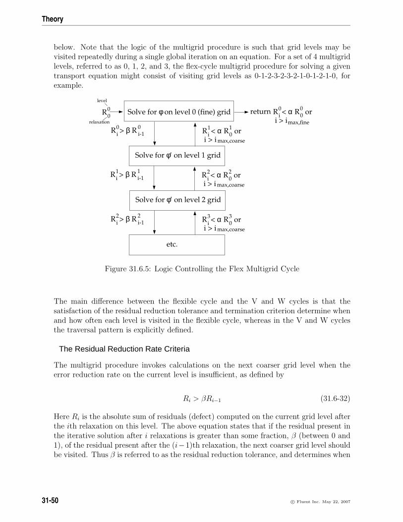
Theory
below. Note that the logic of the multigrid procedure is such that grid levels may bevisited repeatedly during a single global iteration on an equation. For a set of 4 multigridlevels, referred to as 0, 1, 2, and 3, the flex-cycle multigrid procedure for solving a giventransport equation might consist of visiting grid levels as 0-1-2-3-2-3-2-1-0-1-2-1-0, forexample.
R00 return R < α R or
i > i i0
00
max,fine
Solve for φ on level 0 (fine) grid
R < α R or i > i
i1
01
max,coarse
R > β R i0
i-10
Solve for φ′ on level 1 grid
R < α R or i > i
i2
02
max,coarse
R > β R i1
i-11
Solve for φ′ on level 2 grid
R < α R or i > i
i3
03
max,coarse
R > β R i2
i-12
etc.
level
relaxation
Figure 31.6.5: Logic Controlling the Flex Multigrid Cycle
The main difference between the flexible cycle and the V and W cycles is that thesatisfaction of the residual reduction tolerance and termination criterion determine whenand how often each level is visited in the flexible cycle, whereas in the V and W cyclesthe traversal pattern is explicitly defined.
The Residual Reduction Rate Criteria
The multigrid procedure invokes calculations on the next coarser grid level when theerror reduction rate on the current level is insufficient, as defined by
Ri > βRi−1 (31.6-32)
Here Ri is the absolute sum of residuals (defect) computed on the current grid level afterthe ith relaxation on this level. The above equation states that if the residual present inthe iterative solution after i relaxations is greater than some fraction, β (between 0 and1), of the residual present after the (i−1)th relaxation, the next coarser grid level shouldbe visited. Thus β is referred to as the residual reduction tolerance, and determines when
31-50 c© Fluent Inc. May 22, 2007
31.6 Solution Procedures
to “give up” on the iterative solution at the current grid level and move to solving thecorrection equations on the next coarser grid. The value of β controls the frequency withwhich coarser grid levels are visited. The default value is 0.1. A larger value will resultin less frequent visits, and a smaller value will result in more frequent visits.
The Termination Criteria
Provided that the residual reduction rate is sufficiently rapid, the correction equationswill be converged on the current grid level and the result applied to the solution field onthe next finer grid level.
The correction equations on the current grid level are considered sufficiently convergedwhen the error in the correction solution is reduced to some fraction, α (between 0 and1), of the original error on this grid level:
Ri < αR0 (31.6-33)
Here, Ri is the residual on the current grid level after the ith iteration on this level,and R0 is the residual that was initially obtained on this grid level at the current globaliteration. The parameter α, referred to as the termination criterion, has a default valueof 0.1. Note that the above equation is also used to terminate calculations on the lowest(finest) grid level during the multigrid procedure. Thus, relaxations are continued on eachgrid level (including the finest grid level) until the criterion of this equation is obeyed(or until a maximum number of relaxations has been completed, in the case that thespecified criterion is never achieved).
Restriction, Prolongation, and Coarse-Level Operators
The multigrid algorithm in Airpak is referred to as an “algebraic” multigrid (AMG)scheme because, as we shall see, the coarse level equations are generated without theuse of any geometry or re-discretization on the coarse levels; a feature that makes AMGparticularly attractive for use on unstructured meshes. The advantage is that no coarsegrids have to be constructed or stored, and no fluxes or source terms need be evaluated onthe coarse levels. This approach is in contrast with FAS (sometimes called “geometric”)multigrid in which a hierarchy of meshes is required and the discretized equations areevaluated on every level. In theory, the advantage of FAS over AMG is that the formershould perform better for non-linear problems since non-linearities in the system arecarried down to the coarse levels through the re-discretization; when using AMG, oncethe system is linearized, non-linearities are not “felt” by the solver until the fine leveloperator is next updated.
c© Fluent Inc. May 22, 2007 31-51

Theory
AMG Restriction and Prolongation Operators
The restriction and prolongation operators used here are based on the additive correction(AC) strategy described for structured grids by Hutchinson and Raithby [13]. Inter-leveltransfer is accomplished by piecewise constant interpolation and prolongation. The defectin any coarse level cell is given by the sum of those from the fine level cells it contains,while fine level corrections are obtained by injection of coarse level values. In this mannerthe prolongation operator is given by the transpose of the restriction operator
P = RT (31.6-34)
The restriction operator is defined by a coarsening or “grouping” of fine level cells intocoarse level ones. In this process each fine level cell is grouped with one or more ofits “strongest” neighbors, with a preference given to currently ungrouped neighbors.The algorithm attempts to collect cells into groups of fixed size, typically two or four,but any number can be specified. In the context of grouping, strongest refers to theneighbor j of the current cell i for which the coefficient Aij is largest. For sets of coupledequations Aij is a block matrix and the measure of its magnitude is simply taken to bethe magnitude of its first element. In addition, the set of coupled equations for a givencell are treated together and not divided amongst different coarse cells. This results inthe same coarsening for each equation in the system.
AMG Coarse Level Operator
The coarse level operator AH is constructed using a Galerkin approach. Here we re-quire that the defect associated with the corrected fine level solution must vanish whentransferred back to the coarse level. Therefore we may write
Rdnew = 0 (31.6-35)
Upon substituting Equations 31.6-25 and 31.6-31 for dnew and φnew we have
R [Aφnew + b] = 0
R[A(φ+ P ψH
)+ b
]= 0 (31.6-36)
Now rearranging and using Equation 31.6-25 once again gives
RAP ψH +R (Aφ+ b) = 0
RAP ψH +Rd = 0 (31.6-37)
31-52 c© Fluent Inc. May 22, 2007

31.6 Solution Procedures
Comparison of Equation 31.6-37 with Equation 31.6-30 leads to the following expressionfor the coarse level operator:
AH = RAP (31.6-38)
The construction of coarse level operators thus reduces to a summation of diagonal andcorresponding off-diagonal blocks for all fine level cells within a group to form the diagonalblock of that group’s coarse cell.
31.6.5 Solution Residuals
During the solution process you can monitor the convergence dynamically by checkingresiduals. At the end of each solver iteration, the residual sum for each of the conservedvariables is computed and stored, thus recording the convergence history. This historyis also saved in the data file. The residual sum is defined below.
On a computer with infinite precision, these residuals will go to zero as the solutionconverges. On an actual computer, the residuals decay to some small value (“round-off”) and then stop changing (“level out”). For “single precision” computations (thedefault for workstations and most computers), residuals can drop as many as six ordersof magnitude before hitting round-off. Double precision residuals can drop up to twelveorders of magnitude. Guidelines for judging convergence can be found in Section 27.12.5.
After discretization, the conservation equation for a general variable φ at a cell P can bewritten as
aPφP =∑nb
anbφnb + b (31.6-39)
Here aP is the center coefficient, anb are the influence coefficients for the neighboringcells, and b is the contribution of the constant part of the source term Sc in S = Sc+SPφand of the boundary conditions. In Equation 31.6-39,
aP =∑nb
anb − SP (31.6-40)
The residual Rφ computed by Airpak is the imbalance in Equation 31.6-39 summed overall the computational cells P . This is referred to as the “unscaled” residual. It may bewritten as
Rφ =∑
cells P
|∑nb
anbφnb + b− aPφP | (31.6-41)
c© Fluent Inc. May 22, 2007 31-53

Theory
In general, it is difficult to judge convergence by examining the residuals defined byEquation 31.6-41 since no scaling is employed. This is especially true in enclosed flowssuch as natural convection in a room where there is no inlet flow rate of φ with which tocompare the residual. Airpak scales the residual using a scaling factor representative ofthe flow rate of φ through the domain. This “scaled” residual is defined as
Rφ =
∑cells P
∣∣∣∣∣∑nb
anbφnb + b− aPφP∣∣∣∣∣∑
cells P
|aPφP |(31.6-42)
For the momentum equations the denominator term aPφP is replaced by aPvP , where vPis the magnitude of the velocity at cell P .
The scaled residual is a more appropriate indicator of convergence, and is the residualdisplayed by Airpak.
For the continuity equation, the unscaled residual is defined as
Rc =∑
cells P
|rate of mass creation in cell P| (31.6-43)
The scaled residual for the continuity equation is defined as
Rciteration N
Rciteration 5
(31.6-44)
The denominator is the largest absolute value of the continuity residual in the first fiveiterations.
31-54 c© Fluent Inc. May 22, 2007

Bibliography
[1] ASHRAE. ASHRAE Handbook – 1997 Fundamentals. American Society of Heating,Refrigerating, and Air-Conditiong Engineers, Alanta, Georgia, 1997.
[2] T. J. Barth and D. Jespersen. The design and application of upwind schemes on un-structured meshes. Technical Report AIAA-89-0366, AIAA 27th Aerospace SciencesMeeting, Reno, Nevada, 1989.
[3] G. K. Batchelor. An Introduction to Fluid Dynamics. Cambridge Univ. Press,Cambridge, England, 1967.
[4] H. C. Chen and V. C. Patel. Near-Wall Turbulence Models for Complex FlowsIncluding Separation. AIAA Journal, 26(6):641–648, 1988.
[5] Q. Chen and J. Srebric. Simplified Diffuser Boundary Conditions for NumericalRoom Airflow Models. ASHRAE RP-1009, 2000.
[6] D. Choudhury. Introduction to the Renormalization Group Method and TurbulenceModeling. Fluent Inc. Technical Memorandum TM-107, 1993.
[7] E. H. Chui and G. D. Raithby. Computation of Radiant Heat Transfer on a Non-Orthogonal Mesh Using the Finite-Volume Method. Numerical Heat Transfer, PartB, 23:269–288, 1993.
[8] M. F. Cohen and D. P. Greenberg. The hemi-cube: a radiosity solution for complexenvironments. Computer Graphics, 19(3):31–40, 1985.
[9] J. Dacles-Mariani, G. G. Zilliac, J. S. Chow, and P. Bradshaw. Numeri-cal/Experimental Study of a Wingtip Vortex in the Near Field. AIAA Journal,33(9):1561–1568, 1995.
[10] R. A. W. M. Henkes, F. F. van der Flugt, and C. J. Hoogendoorn. Natural Con-vection Flow in a Square Cavity Calculated with Low-Reynolds-Number TurbulenceModels. Int. J. Heat Mass Transfer, 34:1543–1557, 1991.
[11] J.O. Hinze. Turbulence. McGraw-Hill Publishing Co., New York, 1975.
[12] P. Huang, P. Bradshaw, and T. Coakley. Skin Friction and Velocity Profile Fam-ily for Compressible Turbulent Boundary Layers. AIAA Journal, 31(9):1600–1604,September 1993.
c© Fluent Inc. May 22, 2007 Bib-1

Bibliography
[13] B. R. Hutchinson and G. D. Raithby. A Multigrid Method Based on the AdditiveCorrection Strategy. Numerical Heat Transfer, 9:511–537, 1986.
[14] I. E. Idelchick. Handbook of Hydraulic Resistances. Hemisphere Publishing Corp.,2nd edition, 1986.
[15] T. Jongen. Simulation and Modeling of Turbulent Incompressible Flows. PhD thesis,EPF Lausanne, Lausanne, Switzerland, 1992.
[16] B. Kader. Temperature and Concentration Profiles in Fully Turbulent BoundaryLayers. Int. J. Heat Mass Transfer, 24(9):1541–1544, 1993.
[17] G. Karypis and V. Kumar. METIS - A Software Package for Partitioning Un-structured Graphs, Partitioning Meshes, and Computing Fill-Reducing Orderingsof Sparse Matrices, Version 3.0. Manual, University of Minnesota and Army HPCResearch Center, 1997.
[18] W. M. Kays. Turbulent Prandtl Number - Where Are We? J. Heat Transfer,116:284–295, 1994.
[19] B. E. Launder and D. B. Spalding. Lectures in Mathematical Models of Turbulence.Academic Press, London, England, 1972.
[20] M. F. Modest. Radiative Heat Transfer. Series in Mechanical Engineering. McGrawHill, 1993.
[21] J. Y. Murthy and S. R. Mathur. A Finite Volume Method For Radiative HeatTransfer Using Unstructured Meshes. AIAA-98-0860, January 1998.
[22] S. V. Patankar. Numerical Heat Transfer and Fluid Flow. Hemisphere, Washington,D.C., 1980.
[23] G. D. Raithby and E. H. Chui. A Finite-Volume Method for Predicting a RadiantHeat Transfer in Enclosures with Participating Media. J. Heat Transfer, 112:415–423, 1990.
[24] C. M. Rhie and W. L. Chow. Numerical Study of the Turbulent Flow Past an Airfoilwith Trailing Edge Separation. AIAA Journal, 21(11):1525–1532, November 1983.
[25] J. A. Snyman. A New and Dynamic Method for Unconstrained Minimization. Ap-plied Mathematical Modeling, 6:449–462, 1982.
[26] J. A. Snyman. An improved Version of the Original Leap-Frog Method for Uncon-strained Minimization. Applied Mathematical Modeling, 7:216–218, 1983.
[27] J. A. Snyman. The LFOPC Leap-Frog Algorithm for Constrained Optimization.Computers and Mathematics with Applications, 40:1085–1096, 2000.
Bib-2 c© Fluent Inc. May 22, 2007

Bibliography
[28] J. A. Snyman, W. J. Roux, and N. Stander. A Dynamic Penalty Function Method forthe Solution of Structural Optimization Problems. Applied Mathematical Modeling,18:453–460, 1994.
[29] P. Spalart and S. Allmaras. A one-equation turbulence model for aerodynamic flows.Technical Report AIAA-92-0439, American Institute of Aeronautics and Astronau-tics, 1992.
[30] F. White and G. Christoph. A Simple New Analysis of Compressible TurbulentSkin Friction Under Arbitrary Conditions. Technical Report AFFDL-TR-70-133,February 1971.
[31] M. Wolfstein. The Velocity and Temperature Distribution of One-Dimensional Flowwith Turbulence Augmentation and Pressure Gradient. Int. J. Heat Mass Transfer,12:301–318, 1969.
[32] V. Yakhot and S. A. Orszag. Renormalization Group Analysis of Turbulence: I.Basic Theory. Journal of Scientific Computing, 1(1):1–51, 1986.
c© Fluent Inc. May 22, 2007 Bib-3

Bibliography
Bib-4 c© Fluent Inc. May 22, 2007

Index
1/4 Polygonal cylinder panel, 25-511/4 polygonal cylinder macro, 25-51
Accept button, 2-42accuracy
diffusion terms, 31-39first-order, 27-5, 31-39second-order, 27-5, 31-39
Active, 7-43Active parameter panel, 24-5activity level, 30-8Add marker panel, 2-8adding objects to a group, 7-69Adobe Acrobat Reader, 1-23ADPI button, 29-20ADPI reports, 29-20ADPI specification panel, 29-20Advanced parameters button, 26-15Advanced solver setup panel, 27-4air inlet diffuser, 25-10Airpak environment variables, 1-16airpak, 1-11airpak -unpack, 1-15airpak -x, 1-15airpak -xfast, 1-15airpak projectname, 1-15AIRPAK JOB DIRECTORY, 1-16AIRPAK LIB PATH, 1-16AIRPAK LICENSE FILE, 1-16algebraic multigrid (AMG), 31-40, 31-45Align and morph edges button, 2-31Align and morph faces button, 2-31Align and morph vertices button, 2-31Align centers button, 7-36Align edges button, 7-33Align face centers button, 2-31, 7-36Align faces button, 7-32
Align object centers button, 2-31Align vertices button, 7-35All projects button, 6-12, 6-19ambient values, 6-39angular deviation, 29-3, 30-2Angular deviation panel, 30-2angular discretization, 31-26animated GIF files, 28-17, 28-24animation
isosurface, 28-22particle traces, 28-41plane cut, 28-15saving, 28-16, 28-23transient simulations, 20-21
Anisotropic tensor panel, 7-78annotations, 2-36, 6-15Annotations panel, 2-36applications, 1-8Assemblies, 7-90Assemblies panel, 7-91assembly, see also object, 7-90
adding objects to, 7-91copying, 7-96creating, 7-90
using a group, 7-73deleting, 7-98editing, 7-91, 7-96expanding into its components, 7-98external, 7-92internal, 7-93loading, 7-97merging, 7-97meshing, 26-29moving, 7-97saving, 7-97selecting, 7-96
c© Fluent Inc. May 22, 2007 Index-1

Index
summary, 7-98total area, 7-99total volume, 7-99translating, 7-93viewing, 7-96
Assembly contents panel, 7-98Assembly node, 2-57atmospheric boundary layer macro, 25-4,
25-6northward direction, 6-39, 25-6wind direction, 25-6wind speed, 25-8
Atmospheric boundary layer panel, 25-6augmentation efficiency, 21-9automatic mesh generation, 26-1Autoscale button, 7-9Available toolbars panel, 2-47
background color, 2-9baffles, 10-2band width for contour plots, 28-33Basic parameters panel, 6-27Basic settings panel, 27-7
Reset button, 6-39, 27-5, 27-8transient simulations, 20-11
batch execution, 27-26batch file, 27-26block, see also object, 8-1
additional resistance, 8-13combination, 8-3, 8-8
coincident surfaces, 8-3intersecting volumes, 8-4
creating, 8-9fixed heat, 8-3fixed temperature, 8-3fluid, 8-2, 8-14hollow, 8-2, 8-16individual sides, 8-3, 8-11meshing, 26-21
3D polygon, 26-22cylinder, 26-22ellipsoid, 26-23elliptical cylinder, 26-23prism, 26-21
on external wall, 8-7partition
intersecting volume, 8-7surface coincident, 8-6
radiation, 8-11, 22-2emissivity, 22-7specification, 22-5
solid, 8-2, 8-14species, 21-6surface roughness, 8-2thermal properties, 8-2, 8-3, 8-13, 8-14transient simulations, 8-16, 20-9type, 8-2
Block thermal conditions panel, 8-16, 8-17Blocks panel, 8-9blower, see also object
operating point, 29-19body forces, 31-42boundary conditions
parameterization, 24-1radiation
discrete ordinates (DO) model, 31-29,31-30
radiative heat transfer, 13-7solar flux, 25-2species, 21-6, 21-8turbulence
input methods, 6-33boundary layer, 25-4boundary profiles, 11-11, 13-19
species mass fraction, 21-11Boussinesq approximation, 6-36, 31-22Boussinesq hypothesis, 31-7box method, 25-11Box method parameters panel, 25-44browser, 1-18bubble help, 2-49, 6-17building a model, 7-1buoyancy forces, 31-21
CAD data operation options panel, 4-3, 4-16CAD data panel, 4-3CAD geometry, 4-1calculating a solution, 27-1, 27-49
Index-2 c© Fluent Inc. May 22, 2007

Index
in batch mode, 27-26using RSF, 27-29
Cancel button, 2-43capabilities, 1-4
boundary conditions, 1-7general, 1-4materials, 1-6meshing, 1-5model building, 1-4physical models, 1-6reporting, 1-8solver, 1-7visualization, 1-7
case files, 3-3, 27-20ceiling diffuser, 25-12cell values, 31-39check box, 2-43Check model button, 2-27checking the design, 7-99checking the mesh, 26-39
element quality, 26-39element volume, 26-42face alignment, 26-41
circular object, 7-47meshing, 26-24
Clean up project data panel, 3-17cleaning up project data, 3-16closed box macro, 25-48Closed box panel, 25-48clothing, 30-7co-located scheme, 31-41coarse mesh
hexahedral, 26-5tetrahedral, 26-7
coarsening the mesh, 26-14cocooning, 26-2, 26-12color, 6-20
contour plot, 28-33graphical displays, 28-5group, 7-68object, 7-43particle trace, 28-43room, 7-13
vector plot, 28-37color legend
data format, 6-12moving, 2-61
color levelscontour plot, 28-34
color spectrum, 28-5changing, 2-61contour plot, 28-34data format, 6-12
comfort level, 6-30variables, 30-6
postprocessing, 6-32Comfort level button, 30-7Comfort level panel, 30-7compass orientation of model, 6-39compressing project data, 3-16compute nodes, 27-21computing view factors, 22-10
adaptive method, 22-11hemicube method, 22-11
condenser, 17-1conduction, 31-2
transient simulations, 20-1configuring a project, 6-11conjugate-gradient methods, 31-45conservation equations
discretization, 31-38integral form, 31-41
Contents button, 1-20context-specific help, 2-49continuity equation, 31-1contours, 28-31control panels, 2-42control volume technique, 31-36convection, 31-21
forced, 6-36natural, 6-36transient simulations, 20-1
conventions used in this manual, UTM-5convergence, 31-53
criteria, 27-7, 31-36history, 27-49
c© Fluent Inc. May 22, 2007 Index-3

Index
judging, 27-52, 31-53monitoring, 27-51
conversion factorsunits, 5-7
coordinate axesmoving, 2-61
coordinate systems, 7-28Copy assembly panel, 7-96Copy from button, 7-41Copy group panel, 7-71Copy object button, 2-31, 7-38, 7-82, 7-96Copy object panel, 7-38copying
assembly, 7-96group, 7-71materials, 7-81mesh data, 3-10meshing parameters, 26-19object, 7-38, 7-41solution data, 3-10
Create assemblies button, 2-30, 7-91Create blocks button, 2-29, 8-9Create fans button, 2-29, 9-11Create heat exchangers button, 2-30, 17-3Create hoods button, 2-30, 18-3Create image file button, 2-25, 6-4Create materials button, 2-30, 7-82Create openings button, 2-29, 11-6Create partitions button, 2-29, 14-4Create persons button, 2-29, 12-3Create resistances button, 2-30, 16-4Create sources button, 2-29, 15-3Create vents button, 2-29, 10-6Create walls button, 2-29, 13-10Create wires button, 2-30, 19-1creating
assembly, 7-90block, 8-9fan, 9-11group, 7-67heat exchanger, 17-3hood, 18-3isosurface, 28-22
local coordinate system, 7-28materials, 7-82named point, 20-25object, 7-19object face, 28-11opening, 11-6partition, 14-4person, 12-3plane cut, 28-15point, 28-29project, 6-7resistance, 16-4room, 7-4source, 15-3vent, 10-6wall, 13-10wire, 19-1
cross-sectiondisplaying results, 28-12displaying the mesh, 26-36
CSV/Excel files, 4-20, 4-25, 4-28Curve specification panel, 7-88, 9-15, 10-15,
11-11, 13-19, 20-17, 21-11custom assembly, 7-90customizing
materials, 7-75, 7-83mesh parameters, 26-1units, 5-4
cylinder, 7-56elliptical, 7-59
meshing, 26-23meshing, 26-13, 26-16, 26-22
cylinder plate macro, 25-53cylinder plate panel, 25-53cylindrical enclosure macro, 25-55Cylindrical enclosure panel, 25-55
data files, 3-4date, 2-61default materials, 6-40Define point report panel, 29-13Define summary report panel, 27-13, 29-9defining
isosurface, 28-21
Index-4 c© Fluent Inc. May 22, 2007

Index
object face, 28-9plane cut, 28-12point, 28-27postprocessing objects, 27-13project, 6-1summary report, 27-13, 29-11
Delete object button, 2-30, 7-84, 7-98, 28-8deleting
assembly, 7-98CAD geometry, 4-18group, 7-72isosurface, 28-26local coordinate system, 7-30materials, 7-84named point, 20-26object, 7-20object face, 28-12parameters, 24-10plane cut, 28-19point, 28-29postprocessing objects, 28-7project, 6-10
density, 7-77, 7-79, 21-2incompressible ideal gas law, 31-22
derived variables, 29-1, 30-1deselecting
object, 7-19design
checking, 7-99optimization, 24-1
design variablecreating a new design variable, 24-9
diagnosticfiles, 3-4tools, 27-52
diffuser macro, 25-10box method, 25-11modeling methods, 25-10momentum method, 25-11types, 25-12using, 25-12
Diffuser panel, 25-10diffusion coefficient, 21-2, 31-3
diffusion species, 31-3diffusivity, 7-79discrete ordinates (DO) radiation model,
31-26angular discretization, 31-26boundary conditions
flow inlets and exits, 31-30symmetry boundaries, 31-30walls, 31-29
pixelation, 31-26using, 22-14
discrete valuesstorage points, 31-39
discretization, 27-4, 31-38, 31-44first-order scheme, 31-39pressure interpolation schemes, 27-5,
31-41second-order scheme, 31-39spatial, 31-38temporal, 31-44
displacement diffuser, 25-12DISPLAY, 1-16Display object names button, 2-26displaying
mesh, 26-32cross-section, 26-36individual objects, 26-32
residuals, 27-12results, 28-1view factors, 22-11
divergence, 27-5DO radiation model, 31-26documentation, 1-17double precision, 31-53double-precision solvers, 27-7Download RSF project button, 2-28drop-down list, 2-45DWG files, 4-20, 4-23DXF files, 4-20, 4-21dynamic head, 17-1dynamic-q optimization method, 23-1, 31-
30
Edit button, 7-4
c© Fluent Inc. May 22, 2007 Index-5

Index
Edit commands toolbar, 2-25Edit menu, 2-5Edit object button, 2-30Edit units button, 5-9Edit window, 1-13, 2-38Edit window
object, 7-14room, 7-4
Edit/Annotations, 2-6Edit/Current group, 2-6, 7-65Edit/Current group/Activate all, 2-7, 7-73Edit/Current group/Add to group, 2-6, 7-69Edit/Current group/Copy, 2-7, 7-71Edit/Current group/Copy params, 2-7, 7-71Edit/Current group/Create, 2-6, 7-67Edit/Current group/Create assembly, 2-7, 7-
73, 7-90Edit/Current group/Deactivate all, 2-7, 7-73Edit/Current group/Delete, 2-6, 7-72Edit/Current group/Delete all, 2-7, 7-73Edit/Current group/Edit, 2-7, 7-72Edit/Current group/Move, 2-7Edit/Current group/Remove from group, 2-6,
7-70Edit/Current group/Rename, 2-6, 7-67Edit/Current group/Save as project, 2-7, 7-73Edit/Current object, 2-6Edit/Current object/Active, 2-6Edit/Current object/Copy, 2-6Edit/Current object/Copy from, 2-6Edit/Current object/Delete, 2-6Edit/Current object/Edit, 2-6Edit/Current object/Modify, 2-6Edit/Current object/Move, 2-6Edit/Current object/Remove from group, 2-6Edit/Current object/Reset, 2-6Edit/Preferences, 2-6Edit/Redo, 2-6Edit/Undo, 2-6editing
assembly, 7-91, 7-96interactively, 6-23isosurface, 28-22
local coordinate system, 7-29materials, 7-75named point, 20-25object, 7-19object face, 28-11plane cut, 28-15point, 28-29postprocessing objects, 28-7view factors, 22-13
elementcount, 26-18height, 26-18quality, 26-39volume, 26-42
ellipsoid, 7-58meshing, 26-5, 26-23
elliptical cylinder, 7-59meshing, 26-5, 26-23
Email Project panel, 27-53emailing a project, 27-53emissivity, 7-80, 22-2, 22-14enclosure, see also objectenergy equation, 31-2environment variables, 1-15
Airpak, 1-16system, 1-15
Epsilon, 29-3error reduction, 31-45, 31-46
rate, 31-50examining
mesh, 26-32, 26-39hexahedral, 26-5tetrahedral, 26-7
results, 28-1exhaust hood, 18-1Exhaust species concentration panel, 25-45exiting, 2-64exporting
CAD geometry, 4-1, 4-28CSV/Excel files, 4-28IGES files, 4-28mesh, 26-44STEP files, 4-28
Index-6 c© Fluent Inc. May 22, 2007

Index
tetin files, 4-28exporting solution data, 27-21external assembly, 7-92
F1 key, 2-49F9 key, 2-62face alignment, 26-41face flow rate, 31-42families, 4-6
converting into Airpak objects, 4-10moving CAD geometry between, 4-7visibility, 4-17
fan, see also object, 9-1characteristic curve, 9-1, 9-9, 9-14, 9-15circular, 9-3combination
parallel, 9-6series, 9-6
creating, 9-11exhaust, 9-2, 9-4, 9-9, 9-12fixed flow, 9-1, 9-8flow, 9-1flow direction, 9-4, 9-12flow rate, 9-12hub, 9-1, 9-3intake, 9-2, 9-4, 9-9, 9-12internal, 9-2, 9-4, 9-9, 9-13located on a block, 9-7meshing, 26-24operating point, 29-19pressure drop, 9-9rectangular, 9-3RPM, 9-8species, 21-6static pressure, 9-9swirl magnitude, 9-8transient simulations, 9-2, 9-14, 20-9turbulence parameters, 9-14
Fan curve window, 9-14Fans panel, 9-11File commands toolbar, 2-24, 6-3File menu, 2-2, 6-1File selection dialog box, 2-39File/Cleanup, 2-5, 3-17, 6-3
File/Command prompt, 2-5, 6-3File/Create image file, 2-5, 6-3File/Email project, 2-5, 6-3, 27-53File/Export, 2-4, 6-2File/Import, 2-4, 4-1, 6-2File/Merge project, 2-4, 3-5, 6-2File/New project, 2-3, 6-1, 6-7File/Open project, 2-4, 6-1, 6-8File/Pack, 27-53File/Pack project, 2-5, 3-16, 6-2File/Print screen, 2-5, 6-3File/Quit, 2-5, 6-3File/Reload main version, 2-4, 6-2, 6-9File/Save project, 2-4, 3-9, 6-2File/Save project as, 2-4, 3-9, 6-2File/Shell window, 2-5, 6-3File/Unpack project, 2-4, 3-16, 6-2files
Airpak, 3-3AVI, 28-17, 28-24batch, 27-26case, 3-3, 27-20CSV/Excel, 4-20, 4-25, 4-28data, 3-4diagnostic, 3-4DWG, 4-20, 4-23DXF, 4-20, 4-21exporting, 4-1, 4-28Flash, 28-18, 28-25FLI, 28-17, 28-24GIF
animated, 28-17, 28-24grid, 3-3HTML, 1-18IFC, 4-23IGES, 4-2, 4-20, 4-21image, 3-10
format, 3-14frame, 3-15label, 3-15landscape, 3-12portrait, 3-12PostScript options, 3-14
c© Fluent Inc. May 22, 2007 Index-7

Index
scaling, 3-12importing, 4-1job, 3-3log, 2-38mesh, 3-3model, 3-3MPEG, 28-17, 28-24node, 27-23opening, 2-39optimization, 3-4
input, 3-4log, 3-4output, 3-4postprocessing, 3-4tab, 3-4
overview, 3-1PDF, 1-23postprocessing, 3-4PostScript, 3-14, 6-16problem, 3-3problem setup, 3-3reading, 2-39residual, 3-4, 27-53saving, 2-39
transient simulations, 20-4scratch, 3-18script, 3-4, 27-20selecting, 2-39solution, 3-18solver, 3-3
input, 3-4output, 3-4
STEP, 4-2tetin, 4-2, 4-3version, 3-18writing, 2-39
filter efficiency, 21-9Find in tree panel, 2-16finite-volume scheme, 31-38first-order accuracy, 27-5, 31-39Fix shapes, 12-5, 18-3Fix values, 5-6flex-cycle multigrid, 31-49
floating toolbars, 2-47flow
heat, 29-3, 30-3mass, 29-3, 30-2radiative heat, 29-3regime, 6-32variables, 6-29
postprocessing, 6-31volume, 29-4, 30-2
Flow dependent heat transfer panel, 13-16FLUENT, 1-1, 1-7fluid material
default, 6-40properties, 7-78
fluxheat, 29-3, 30-3
radiation, 22-2font, 6-22forced convection, 6-29, 6-36forces
inertial, 6-39viscous, 6-39
Form factors panel, 22-8Four viewing windows button, 2-26fraction menu, 21-5frame
image, 3-15Full report panel, 29-15
gas law, 31-22Gauss-Seidel method, 31-45Generate mesh button, 2-27, 5-2, 26-8, 26-10geometric transformations
for merging model data, 3-6object, 7-22, 7-39room, 7-8, 7-10
geometryobject, 7-45parameterization, 24-1
governing equations, 31-1discretization, 31-38integral form, 31-41
Graph editor, 7-86, 9-14, 10-13, 20-15graphical displays, 28-5
Index-8 c© Fluent Inc. May 22, 2007

Index
color, 28-5graphical styles
editing, 6-20graphical user interface (GUI), 2-1
configuring, 6-11graphics display and control window, 2-34graphics driver, 1-15Graphics file options panel, 3-14graphics tools for postprocessing, 28-1Graphics window, 1-13graphics window, 2-33
adding annotations, 2-36adding arrows, 2-36adding lines, 2-37adding markers, 2-8, 2-37adding text, 2-37background color, 2-9isometric view, 2-14, 2-27lighting options, 2-12scale to fit, 2-14, 2-26views, 2-13zooming, 2-14, 2-26, 2-64
Grashof number, 31-21gravity, 6-37grid, see also mesh, 26-1
files, 3-3storage points, 31-39
grille diffuser, 25-12group, 7-65
activating, 7-73adding objects, 7-69color, 7-68copying, 7-71creating, 7-67
assembly, 7-73, 7-90from imported IGES geometry, 4-16
deactivating, 7-73deleting, 7-72displaying results, 28-9editing object properties, 7-72including objects, 7-43line width, 7-68moving, 7-72
removing objects, 7-70renaming, 7-67saving, 7-73shading, 7-68texture, 7-69transparency, 7-69
Group parameters panel, 7-67Groups node, 2-51, 6-6GUI, 2-1
configuring, 6-11
heat exchanger, see also object, 17-1creating, 17-3heat transfer, 17-2heat transfer coefficient, 17-2meshing, 26-29pressure drop, 17-1
Heat exchangers panel, 17-3heat flow, 29-3, 30-3heat flux, 29-3, 30-3
radiation, 22-2heat sink, see also objectheat sources, 17-1, 31-2Heat tr. coeff parameters panel, 30-4Heat tr. coeff, 29-4, 30-4heat transfer, 22-1, 31-2
conducting solids, 31-2heat transfer coefficient, 17-2, 29-4, 30-4heaters, 11-1help, 1-17, 2-48
bubble, 2-49context-specific, 2-49F1 key, 2-49on-line, 2-48
Help menu, 2-24Help/Airpak on the Web, 2-24Help/Help, 2-24Help/List shortcuts, 2-24Help/User Services Center, 2-24hemisphere macro, 25-63Hemisphere panel, 25-63hex-dominant mesh, 26-4hexahedral mesh, see also mesh, 26-4hidden line removal, 2-10
c© Fluent Inc. May 22, 2007 Index-9

Index
high end, 26-19high side, 26-19High side surface properties panel, 14-12History plot button, 2-28, 20-23, 28-4history plot for transient simulations, 20-22History plot panel, 20-23HOME, 1-16Home position button, 2-26hood, 18-1
creating, 18-3exhaust, 18-1Fix shapes option, 18-3flow rate, 18-3, 18-7meshing, 26-29
Hoods panel, 18-3Hoods shape data panel, 18-5HTML files, 1-18HTML report, 29-5HTML report panel, 29-5hub, 9-3humidity, 29-3, 30-6, 30-8humidity ratio, 21-5hydraulic diameter, 6-35
I-deas, 27-21IAQ, 6-30
variables, 30-6postprocessing, 6-32
ideal gas law, 6-37, 31-22IFC files, 4-23IGES files, 4-2, 4-20, 4-21
exporting, 4-28IGES geometry
blanking surfaces, 4-17converting families into Airpak objects,
4-10converting regions into Airpak objects,
4-11converting selected CAD geometry into
Airpak objects, 4-9deleting CAD geometry, 4-18families, 4-6
moving CAD geometry between, 4-7visibility, 4-17
fixing small gaps, 4-19groups, 4-16importing into Airpak, 4-3manipulating with mouse, 4-19minimum feature size, 4-16options, 4-16overview, 4-2selecting CAD geometry, 4-7shading CAD surfaces, 4-19unblanking surfaces, 4-17unused CAD geometry, 4-17used CAD geometry, 4-17
image, 3-10, 3-12file format, 3-14frame, 3-15label, 3-15landscape, 3-12options, 3-10portrait, 3-12PostScript options, 3-14scaling, 3-12
importingCAD geometry, 4-1CSV/Excel files, 4-20, 4-25DWG files, 4-20, 4-23DXF files, 4-20, 4-21IDF files, see also IDF filesIFC files, 4-23IGES files, see also IGES geometry, 4-2,
4-20, 4-21overview, 4-1STEP files, 4-2tetin files, 4-2, 4-3
improving the meshhexahedral, 26-6tetrahedral, 26-7
Inactive node, 2-54, 6-6inclined object, 7-48
meshing, 26-26Index button, 1-20individual plate macro, 25-65Individual polygonal blocks panel, 25-65, 25-
68
Index-10 c© Fluent Inc. May 22, 2007

Index
Individual prismatic blocks panel, 25-65Individual side specification panel, 8-11indoor air quality, 30-6inertial forces, 6-39initial conditions, 6-41initializing the solution, 27-7interactive editing, 6-23Interactive editing panel, 7-9internal assembly, 7-93interpolation, 31-39, 31-41introduction, 1-1isometric view, 2-14, 2-27Isometric view button, 2-27isosurface
clipping, 28-25displaying results, 28-19
Isosurface button, 2-28, 28-4, 28-21Isosurface contours panel, 28-32Isosurface panel, 28-21Isosurface particles panel, 28-40Isosurface vectors panel, 28-35iterations, 27-7
transient simulations, 20-11iterative procedure, 31-36
job files, 3-3
keyboardshortcuts, 2-62
labelimage, 3-15
laminar flow, 6-32landscape, 3-12Lewis number, 31-3Libraries node, 6-6Library name and info panel, 6-19library path, 6-17Library path panel, 6-17Lighting options panel, 2-12line solvers, 31-45line width, 6-22
contour plot, 28-33group, 7-68
object, 7-43room, 7-13
linearization, 31-37list
drop-down, 2-45single selection, 2-45
Load solution ID button, 2-28, 28-4, 28-51loading
assembly, 7-97existing mesh, 26-45postprocessing objects, 28-8postprocessing views, 28-8report format, 29-7trials plot, 28-51variation plot, 28-47
Local coord systems panel, 7-28local coordinate systems, 7-28
creating, 7-28deleting, 7-30editing, 7-29viewing definition of, 7-30
Local coords panel, 7-29log file, 2-38loss coefficient, 17-1low end, 26-19low side, 26-19Low side surface properties panel, 14-12low-Reynolds-number flows, 31-16Lower pri button, 27-51
macros, 25-11/4 polygonal cylinder, 25-51atmospheric boundary layer, 25-4, 25-6
northward direction, 6-39, 25-6wind direction, 25-6wind speed, 25-8
closed box, 25-48cylinder plate, 25-53cylindrical enclosure, 25-55diffuser, 25-10group of prism blocks, 25-70hemisphere, 25-63individual plate, 25-65polygonal block, 25-68
c© Fluent Inc. May 22, 2007 Index-11

Index
polygonal circle, 25-58polygonal cylinder, 25-62polygonal duct, 25-46prism block, 25-67rotating
group of prism blocks, 25-70polygonal blocks, 25-68prism blocks, 25-67
solar flux, 25-2Macros menu, 2-17, 25-1Macros/1/4 Polygonal cylinder, 25-51Macros/Atmospheric boundary layer, 25-6Macros/Boundary conditions/Atmospheric
boundary layer, 2-18Macros/Boundary conditions/Diffuser, 2-18Macros/Closed box, 25-48Macros/Cylinder plate, 25-53Macros/Cylindrical enclosure, 25-55Macros/Diffuser, 25-10Macros/Ducts/Polygonal ducts, 25-46Macros/Groups of prism blocks, 25-70Macros/Hemisphere, 25-63Macros/Individual Plates, 25-65Macros/Individual polygonal blocks, 25-65,
25-68Macros/Individual prism blocks, 25-67Macros/Individual prismatic blocks, 25-65Macros/Polygonal circle, 25-58Macros/Polygonal cylinder, 25-62Macros/Quick geometry approximations/1/4
Polygonal cylinder, 2-18Macros/Quick geometry approxima-
tions/Closed box, 2-18Macros/Quick geometry approxima-
tions/Cylinder plates, 2-18Macros/Quick geometry approxima-
tions/Cylindrical enclosure, 2-18Macros/Quick geometry approxima-
tions/Hemisphere, 2-18Macros/Quick geometry approxima-
tions/Polygonal circle, 2-18Macros/Quick geometry approxima-
tions/Polygonal cylinder, 2-18
Macros/Quick geometry approxima-tions/Polygonal ducts, 2-18
Macros/Rotate objects/Groups of prismblocks, 2-18
Macros/Rotate objects/Individual plates, 2-18
Macros/Rotate objects/Individual polygonalblocks, 2-18
Macros/Rotate objects/Individual prismblocks, 2-18
Macros/Solar Flux, 25-2Macros/Solar flux, 2-18Main library node, 2-50Main window, 1-12, 2-2managing
postprocessing objects, 28-6manuals, 1-17
printing, 1-23using, 1-18, UTM-1
mass diffusion, 31-3mass diffusion coefficients, 21-2mass flow, 29-3, 30-2mass fraction, 29-3, 30-5
profiles, 21-11Match edges button, 7-38Match faces button, 7-37materials, 7-74
copying, 7-81creating, 7-82default, 6-40deleting, 7-84editing, 7-75fluid, 7-78parameterization, 24-1saving, 7-83solid, 7-77
conductivity, 7-77, 24-3summary, 7-99surface, 7-80temperature dependence, 7-74, 7-85velocity dependence, 7-84viewing properties, 7-81
Materials node, 2-57
Index-12 c© Fluent Inc. May 22, 2007

Index
Materials panel, 7-75, 7-78mean age of air, 29-3, 30-6mean radiant temperature, 6-30, 29-3, 30-6,
30-8Merge project panel, 3-5merging
assembly, 7-97model data, 3-5projects, 3-5
mesh, 26-1checking, 26-39
element quality, 26-39element volume, 26-42face alignment, 26-41
controlling order for objects, 26-30copying, 3-10copying parameters, 26-19displaying, 26-32
cross-section, 26-36individual objects, 26-32
exporting, 26-44files, 3-3, 3-17guidelines, 26-4hex-dominant, 26-4hexahedral, 26-4
coarse, 26-5examining, 26-5improving, 26-6minimum-count, 26-5, 26-8object-specific controls, 26-5parameters, 26-12procedure, 26-5refining, 26-5, 26-11, 26-17
loading, 26-45object-specific controls, 26-17parameters
2D polygon, 26-263D polygon, 26-22assembly, 26-29block, 26-21circular object, 26-24cylinder, 26-22ellipsoid, 26-23
elliptical cylinder, 26-23fan, 26-24heat exchanger, 26-29hood, 26-29inclined object, 26-26opening, 26-26partition, 26-28person, 26-27prism, 26-21rectangular object, 26-25resistance, 26-28room, 26-20source, 26-28vent, 26-24wall, 26-27
partitioning, 27-23planar resistance, 10-3quality, 26-3, 26-39resistance, 16-1skew, 26-3tetrahedral, 26-4
coarse, 26-7coarsening, 26-14examining, 26-7improving, 26-7minimum-count, 26-7, 26-10parameters, 26-15procedure, 26-7refining, 26-7, 26-13, 26-17smoothing, 26-14
units, 5-2Mesh control panel, 5-2, 26-8, 26-10mesh type, 6-24Message window, 1-13, 2-37metabolic rate, 12-3, 30-8METIS, 27-23Min/max locations panel, 28-30minimum-count mesh
hexahedral, 26-5, 26-8tetrahedral, 26-7, 26-10
mirroringmerged model data, 3-7object, 7-22, 7-41
c© Fluent Inc. May 22, 2007 Index-13

Index
room, 7-10model
adding objects, 7-64building, 7-1merging, 3-5northward direction, 6-39, 25-6parameterization, 24-1
Model and solve toolbar, 2-27Model Display window, 2-33model files, 3-3Model manager window
Groups node, 6-6Libraries node, 6-6Problem setup node, 6-4Solution settings node, 6-6
Model manager window, 1-13, 2-31, 6-4Model manager window
collapsing nodes, 6-4expanding nodes, 6-4Inactive node, 6-6Model node, 6-6Points node, 6-6Postprocessing node, 6-6postprocessing objects, 28-6Trash node, 6-6
Model menu, 2-15, 7-4Model node, 2-55, 6-6Model/CAD data, 2-15, 4-3Model/Check model, 2-15, 7-99Model/Create material library, 2-16Model/Edit priorities, 2-15, 26-30Model/Generate mesh, 2-15, 5-2, 26-8, 26-10Model/Radiation, 2-15, 22-8Model/Snap to grid, 2-15Modify form factors panel, 22-13Modify point panel, 27-10mole fraction, 29-3, 30-5molecular weight, 7-79, 21-2momentum equation, 31-2momentum method, 25-11Monitor window, 27-9monitoring
convergence, 31-53
residuals, 31-53solution, 27-8, 27-49, 27-51
Morph edges button, 2-31Morph faces button, 2-31mouse, 2-49
adding objects, 2-60changing color spectrum, 2-61changing controls, 2-61controlling panel inputs, 2-49manipulating graphics, 2-59Model manager window, 2-50
context menus, 2-50moving color legend, 2-61moving coordinate axes, 2-61moving date, 2-61moving title, 2-61resizing objects, 2-61rotating the model, 2-59selecting objects, 2-60switching modes, 2-62translating objects, 2-60translating the model, 2-60zooming the model, 2-60
Move all objects in model panel, 7-8, 7-10Move assembly panel, 7-97Move group panel, 7-72Move object button, 2-31, 7-8, 7-97moving
assembly, 7-97group, 7-72object, 7-21point, 28-28room, 7-9
MPEG file, 28-17, 28-24multigrid solver, 27-6, 31-45
cycles, 31-47flex cycle, 31-49prolongation, 31-47residual reduction rate, 31-49, 31-50restriction, 31-47termination criteria, 31-51V cycle, 31-47, 31-49W cycle, 31-47, 31-49
Index-14 c© Fluent Inc. May 22, 2007

Index
Multiple regions panel, 4-13multiprocessor workstations, 27-22
nameobject, 7-43room, 7-12
named point, 20-24creating, 20-25deleting, 20-26editing, 20-25
Named point panel, 20-24NASTRAN, 27-21natural convection, 6-29, 6-36, 31-42Navier-Stokes equations, 31-1near-wall flows, 31-16network, see also objectnetwork parallel solver, 27-24New directory button, 2-41New project button, 2-24, 6-3New project panel, 1-14New unit name panel, 5-7New/existing panel, 1-12Next button, 1-19node file, 27-23node values, 31-39northward direction, 6-39, 25-6notes, 2-42, 6-8
object, 7-43room, 7-13
nozzle diffuser, 25-12numerical scheme, 31-36
objectadding to group, 7-69aligning
centers, 7-35edges, 7-33face centers, 7-36faces, 7-32matching edges, 7-38matching faces, 7-37vertices, 7-35
aligning with another object, 7-31Edit window, 7-31
Object modification toolbar, 7-31assembly, see also assembly, 7-90attributes, 7-42block, see also block, 8-1blower, see also blowercircular, 7-47color, 7-43controlling meshing order, 26-30copying, 7-38, 7-41copying mesh parameters, 26-19creating, 7-19cylindrical, 7-56deleting, 7-20deselecting, 7-19displaying results, 28-9displaying the mesh, 26-32Edit window, 7-14editing, 7-19editing properties in a group, 7-72ellipsoid, 7-58elliptical cylinder, 7-59emissivity, 22-14enclosure, see also enclosureexcluding, 7-43fan, see also fan, 9-1geometry, 7-45grouping, 7-65heat exchanger, see also heat ex-
changer, 17-1heat sink, see also heat sinkhigh side, 26-19hood, 18-1inclined, 7-48including
in a group, 7-43in model, 7-43
line width, 7-43low side, 26-19minimum separation, 6-24mirroring, 7-22, 7-41moving, 7-21name, 7-43network, see also network
c© Fluent Inc. May 22, 2007 Index-15

Index
notes, 7-43opening, see also opening, 11-1package, see also packageparameterization, 24-1partition, see also partition, 14-1PCB, see also PCBperson, 12-1physical characteristics, 7-63polygon
2D, 7-513D, 7-52
position, 7-44postprocessing
activating, 28-7deactivating, 28-7managing, 28-6
prism, 7-55radiation
modeling, 22-2surface-to-surface model, 22-5
rectangular, 7-45removing from group, 7-70report
full, 29-17summary, 29-12
resistance, see also resistance, 16-1resizing, 7-20rotating, 7-22, 7-41scaling, 7-22, 7-39selecting, 7-19shading, 2-9, 7-44size, 7-44source, see also source, 15-1summary, 7-99texture, 7-44translating, 7-22, 7-41transparency, 7-44vent, see also vent, 10-1wall, see also wall, 13-1wire, see also wire, 19-1
Object creation toolbar, 2-29, 7-1Object face button, 2-28, 28-4, 28-9Object face contours panel, 28-32
Object face panel, 28-9Object face particles panel, 28-40Object face vectors panel, 28-35Object modification toolbar, 2-30, 7-2Object panel, 7-14Object priority panel, 26-30Object selection panel, 7-41object-specific meshing controls, 26-17
hexahedral, 26-5tetrahedral, 26-7
Objects outside panel, 7-22on-line help, 2-48One viewing window button, 2-26Open project button, 2-25, 6-4, 6-8Open project panel, 1-14, 2-39, 6-8opening, see also object, 11-1
creating, 11-6flow direction, 11-4, 11-14free, 11-1, 11-2, 11-8heat flow, 11-4mass flow rate, 11-4, 11-14meshing, 26-26pressure, 11-2profiles, 11-11recirculation, 11-1, 11-3, 11-4, 11-12
mass flow rate, 11-1report, 29-12species, 21-9species filters, 11-5thermal specification, 11-4
species, 11-9, 11-15, 21-6augmentation, 21-9filtering, 21-9
species filters, 11-5temperature, 11-2thermal specification, 11-4, 11-15transient simulations, 11-9, 11-10, 20-10turbulence parameters, 11-9
opening a file, 2-39opening a project, 6-8Openings panel, 11-6operating density, 6-37, 31-22operating point for blower, 29-19
Index-16 c© Fluent Inc. May 22, 2007

Index
operating point for fan, 29-19operating pressure, 6-37, 31-22optimization, 23-1
dynamic-q method, 31-30files, 3-4
input, 3-4log, 3-4output, 3-4postprocessing, 3-4tab, 3-4
specification, 23-2Option parameter panel, 24-8Orient menu, 2-13Orient negative Z button, 2-26Orient positive X button, 2-26Orient positive Y button, 2-26Orient/Clear user views, 2-14, 28-8Orient/Home position, 2-14Orient/Isometric view, 2-14Orient/Nearest axis, 2-14Orient/Orient negative X, 2-14Orient/Orient negative Y, 2-14Orient/Orient negative Z, 2-14Orient/Orient positive X, 2-14Orient/Orient positive Y, 2-14Orient/Orient positive Z, 2-14Orient/Reverse orientation, 2-14Orient/Save user view, 2-14, 28-8Orient/Scale to fit, 2-14Orient/Zoom in, 2-14Orientation commands toolbar, 2-26Output units button, 5-8
package, see also objectradiation, 22-2
packing up a project, 1-15, 3-16, 27-53panels, 2-42parallel processing, 27-21
efficiency, 27-22on a dedicated parallel machine, 27-22on a multiprocessor workstation, 27-22on a workstation cluster, 27-23partitioning, 27-23
Parallel settings panel, 27-22
parallel solver, 27-21Param value panel, 24-4parameterization, 24-1
creating a new parameter, 24-2, 24-9deleting parameters, 24-10trials
defining, 24-11running, 24-13saving, 24-18selecting, 24-13
Parameters and optimization panel, 23-2, 24-9
Parameters and optimization panel, 24-9Parameters and trials panel
selecting trials, 24-11particle trace, 28-39
animation, 28-41partition, see also object, 14-1
additional resistance, 14-12adiabatic thin, 14-1, 14-3, 14-11block surface coincident, 8-6conducting thick, 14-1, 14-3, 14-7conducting thin, 14-1, 14-3, 14-10contact resistance, 14-1, 14-3, 14-9creating, 14-4fluid, 14-1, 14-11high side, 14-2, 14-11hollow thick, 14-1, 14-3, 14-8intersecting block, 8-7low side, 14-2, 14-11meshing, 26-28radiation, 14-13, 22-2
emissivity, 22-7specification, 22-6
surface roughness, 14-4temperature dependence, 14-7, 14-10thermal model, 14-3, 14-7thickness, 14-2transient simulations, 14-8, 20-10using with other objects, 14-4
partitioning the mesh, 27-23Partitions panel, 14-4PATH, 1-16
c© Fluent Inc. May 22, 2007 Index-17
Index
PATRAN, 27-21PCB, see also objectPDF files, 1-23Peclet number, 6-39, 27-8Per-object mesh parameters panel, 26-17Per-object params, 26-17Performance data panel, 25-36person
creating, 12-3Fix shapes option, 12-5location and dimensions, 12-2meshing, 26-27metabolic rate, 12-3position, 12-2, 12-5proportions, 12-2, 12-5radiation, 12-7
emissivity, 22-7specification, 22-6
thermal conditions, 12-3, 12-6person object, 12-1Person shape data panel, 12-6Persons panel, 12-3picture file, 3-17
saving, 2-42, 3-10pixelation, 31-26planar resistance, 10-2plane cut
clipping, 28-18Plane cut button, 2-28, 28-4, 28-12Plane cut contours panel, 28-32Plane cut panel, 28-12Plane cut particles panel, 28-40Plane cut vectors panel, 28-35planning the analysis, 1-9
computational model, 1-9modeling goals, 1-9physical models, 1-9solution procedure, 1-9
PMV, 6-30, 29-3, 30-6point
displaying results, 28-26, 28-29named, 20-24report, 29-13
Point button, 2-28, 28-4, 28-27Point panel, 28-27Point particles panel, 28-40Point vectors panel, 28-35Points node, 2-53, 6-6polygon
2D, 7-513D, 7-52meshing, 26-13
2D, 26-263D, 26-22
polygonal circle macro, 25-58Polygonal circle panel, 25-58polygonal cylinder macro, 25-62Polygonal cylinder panel, 25-62polygonal duct macro, 25-46
meshing, 26-5wire, 19-1
Polygonal ducts panel, 25-46portrait, 3-12position
object, 7-44variables, 30-5
Post menu, 2-21, 28-1Post-processing node, 2-53, 6-6Post/Convergence plot, 2-21, 27-12Post/Create zoom-in model, 2-22, 28-52Post/Download RSF project, 2-22, 28-4Post/History plot, 2-22, 20-23Post/Isosurface, 2-21, 28-21Post/Load post objects from file, 2-22, 28-8Post/Load solution ID, 2-22, 28-51Post/Min/max locations, 2-21Post/Object face, 2-21, 28-9Post/Plane cut, 2-21, 28-12Post/Point, 2-21, 28-27Post/Postprocessing units, 2-22, 5-8Post/Rescale vectors, 2-22, 28-6, 28-8Post/Save post objects to file, 2-22, 28-8Post/Surface probe, 2-21Post/Time average, 2-22, 20-19Post/Transient settings, 2-22, 20-18Post/Trials plot, 2-22, 28-49
Index-18 c© Fluent Inc. May 22, 2007

Index
Post/Variation plot, 2-22, 28-44postprocessing, 28-1
animation, 20-21, 28-41cascade modeling, 28-52color, 28-5contour attributes, 28-31cross-section, 28-12files, 3-4, 3-17graphical displays, 28-5isosurface, 28-19
clipping, 28-25min/max points, 28-30object face, 28-9
defining, 28-9objects
activating, 28-7deactivating, 28-7managing, 28-6Model manager window, 28-6saving, 3-10
particle trace, 28-39plane cut, 28-12
clipping, 28-18defining, 28-12
point, 28-26solution ID, 28-51solution variables, 6-31species transport, 21-12time averaged results, 20-19transient simulations, 20-18
animation, 20-21time averaged results, 20-19
trials plot, 28-47units, 5-8variables, 30-1variation plot, 28-43vectors, 28-35XY plot, 28-43zoom-in modeling, 28-52
postprocessing objectsdefine, 27-13
Postprocessing toolbar, 2-28, 28-4Postprocessing units panel, 5-8
PostScript files, 3-14, 6-16Power and temperature limits button, 2-27PPD, 6-30, 29-3, 30-6Prandtl number, 6-39, 27-8precision, 27-7, 31-53predicted mean vote, 30-6predicted percentage dissatisfied, 30-6preferences
display options, 6-12editing options, 6-14meshing options, 6-24miscellaneous options, 6-17postprocessing options, 6-25printing options, 6-15solution options, 6-25
Preferences and settings panel, 6-11Preferences panel, 5-3pressure, 29-3, 30-2
drop, 17-1interpolation schemes, 27-5, 31-41variable, 30-2
postprocessing, 6-31pressure-correction equation, 31-43pressure-velocity coupling, 31-43Previous button, 1-20primary variables, 29-1, 30-1Print options panel, 2-5, 2-25, 6-3print region, 3-15Print screen button, 2-25, 6-4printed circuit board, see also PCBprinting images, 3-10, 3-12
file format, 3-14frame, 3-15label, 3-15landscape, 3-12portrait, 3-12PostScript options, 3-14print region, 3-15scale, 3-12
printing text files, 6-15printing trials plots, 28-51printing variation plots, 28-47prism, 7-55
c© Fluent Inc. May 22, 2007 Index-19

Index
meshing, 26-21problem files, 3-3problem parameters, 6-26problem setup, 1-10Problem setup node
Basic parameters, 6-4Local coords, 6-6Title/notes, 6-4
profiles, 11-11, 13-19species mass fraction, 21-11
program structure, 1-2project
compressing data, 3-16configuring, 6-11creating, 6-7defining, 6-1deleting, 6-10emailing, 27-53merging, 3-5notes, 6-8opening, 6-8packing up, 1-15, 3-16, 27-53parameters, 6-26reloading, 6-9removing data, 3-16saving, 3-9, 6-7
at specified frequency, 27-21mesh data, 3-10picture files, 3-10postprocessing objects, 3-10solution data, 3-10transient simulations, 20-4
scaling, 6-14title, 6-8unpacking, 1-15, 3-16
prolongation, 31-47push buttons, 2-43
quality of mesh, 26-3, 26-39
radiation, 22-1choosing a model, 22-1discrete ordinates (DO) model, 31-26
using, 22-14
heat flow, 29-3, 30-4heat flux, 22-2solar load model, 22-14specification, 22-4surface-to-surface model, 22-2, 31-24
for individual objects, 22-5objects to include in calculation, 22-
10using Form factors panel, 22-8view factors, 22-10
temperature, 22-3variables, 6-30, 30-4
postprocessing, 6-32Radiation button, 2-27, 22-8Radiation object selection panel, 22-6Radiation specification panel, 22-6radiator, 17-1radio buttons, 2-44Rayleigh number, 6-39, 27-8, 31-21reading a file, 2-39real number entry, 2-44rectangular object, 7-45
meshing, 26-25Redo button, 2-25reference temperature, 30-4refining the mesh
globally, 26-11hexahedral, 26-5, 26-11, 26-17locally, 26-16tetrahedral, 26-7, 26-13, 26-17
refractive index, 31-24refrigeration circuits, 11-1relative humidity, 21-5, 29-3, 30-6, 30-8relaxation scheme, 31-45, 31-49relaxation sweeps, 31-47reloading a project, 6-9Remote execution parameters (via rsh) panel,
27-18Remote Simulation Facility (RSF), 27-29removing
object from group, 7-70project data, 3-16
renaming
Index-20 c© Fluent Inc. May 22, 2007

Index
group, 7-67renormalization group (RNG) theory, 31-16report
solution overview, 29-8Report menu, 2-22, 29-1Report point data panel, 29-14Report summary data panel, 29-10Report window, 29-17Report/ADPI, 29-20Report/ADPI report, 2-23Report/Comfort level, 2-23, 30-7Report/Fan operating points, 2-23, 29-19Report/Full report, 2-23, 29-15Report/HTML report, 2-22, 29-5Report/Point report, 2-23, 29-13Report/Show optimization/param results, 2-
23Report/Solution overview/Create, 2-22, 29-8Report/Solution overview/View, 2-22, 29-8Report/Summary report, 2-23, 29-9reports, 29-1
ADPI, 29-20comfort level, 30-6fan operating point, 29-19full, 29-15
transient simulation, 29-17HTML, 29-5loading format, 29-7point, 29-13
transient simulation, 29-14saving format, 29-7, 29-12, 29-15summary, 27-13, 29-9
transient simulation, 29-10transient simulations, 20-22variables, 29-3, 30-1
rescaling vectors, 28-8Reset button, 2-43residual files, 3-4residual reduction rate criteria, 31-50residuals, 27-7, 27-9, 27-53
definition of, 31-53monitoring, 31-53plotting, 27-12
reduction rate, 31-51scaling of, 31-54
resistance, see also object, 16-1approach velocity, 16-1, 16-2, 16-6creating, 16-4device velocity, 16-1, 16-2, 16-6flow
pressure drop, 16-2free area ratio, 16-1, 16-3heat transfer coefficient, 17-5loss coefficient, 16-1, 16-2, 16-5, 17-2meshing, 16-1, 26-28power law, 16-1, 16-2, 16-6pressure drop, 16-1, 16-2species, 21-7transient simulations, 16-7, 20-11
Resistance curve window, 10-13Resistances panel, 16-4resizing
object, 2-61, 7-20room, 7-5
restarting the solution, 27-15restriction, 31-47Return to Home button, 1-20Reverse orientation button, 2-27Reynolds averaging, 31-6Reynolds number, 6-39, 27-8, 31-21room
color, 7-13creating, 7-4default, 7-4Edit window, 7-4line width, 7-13meshing, 26-20mirroring, 7-10moving, 7-9name, 7-12notes, 7-13resizing, 7-5
to fit objects, 7-9rotating, 7-11scaling, 7-8snap to grid, 7-11
c© Fluent Inc. May 22, 2007 Index-21

Index
translating, 7-11wall, 7-12, 13-1
Room node, 2-56Room panel, 7-5Rotate about screen normal button, 2-26Rotate groups of prism blocks panel, 25-70rotate polygonal block macro, 25-68rotate prism block macro, 25-67Rotate prism blocks panel, 25-67Rotate prism plates panel, 25-65rotated group of prism blocks macro, 25-70rotating
merged model data, 3-7model, 2-59object, 7-22, 7-41room, 7-11
roughness, 7-80round-off error, 31-53RSF
running independent of Airpak, 27-38solve using, 27-29
RSF running from Airpak session, 27-29Run optimization button, 2-27Run solution button, 2-27, 27-8, 27-14
sample session, 1-25Save image panel, 3-10Save object panel, 4-28Save picture file, 2-42Save project button, 2-25, 3-9, 6-4Save project panel, 2-39, 3-9saving
assembly, 7-97contour plot, 28-35fan curve, 9-13, 9-15files, 2-39group, 7-73log files, 2-38materials, 7-83picture file, 2-42, 3-10, 3-17postprocessing objects, 3-10, 28-8postprocessing views, 28-8project, 3-9, 6-7
at specified interval, 27-21
mesh data, 3-10picture file, 3-10postprocessing objects, 3-10solution data, 3-10
reportfull, 29-17point, 29-14summary, 27-17, 29-10
report format, 29-7, 29-12, 29-15resistance curve, 16-6solution data, 27-21trials plot, 28-51variation plot, 28-47vent curve, 10-10, 10-13view factors, 22-13
scalar variables, 30-1scale (in a GUI panel), 2-46Scale to fit button, 2-26scaling
merged model data, 3-6object, 7-22, 7-39project, 6-14room, 7-8vectors, 28-38
Schmidt number, 31-3scratch files, 3-18screens, 10-2script files, 3-4, 27-20Search button, 1-20second-order accuracy, 27-5, 31-39Select family panel, 4-8selecting
assembly, 7-96files, 2-39object, 2-60, 7-19
Selection panel, 7-83sequential solution, 31-36serial solver, 27-22Set range panel, 7-88, 9-15, 10-13, 20-17setting up a problem, 1-10shading, 2-9, 6-22
CAD surfaces, 4-19contour plot, 28-33
Index-22 c© Fluent Inc. May 22, 2007

Index
group, 7-68object, 7-44
SIMPLE algorithm, 31-43single-precision solvers, 27-7single-selection list, 2-45size of an object, 7-44skew, 26-3slider bar, 2-46slot diffuser, 25-12smoothing the mesh, 26-14snap to grid, 7-11Snap to grid panel, 7-11solar flux calculator panel, 25-2solar flux macro, 25-2Solar Load Model parameters panel, 22-15solid material
default, 6-40properties, 7-77
solution, see also solveraccuracy, 31-39batch file, 27-26calculating, 27-1, 27-3, 27-49
on another computer, 27-18cascade modeling, 28-52continuation of, 27-15control, 27-14
advanced options, 27-18convergence, 27-52, 31-53
criteria, 27-7copying data, 3-10diagnostic tools, 27-52discretization scheme, 27-4ending, 27-52examining results of, 28-1initial conditions, 6-41initializing, 27-7monitoring, 27-8, 27-49, 27-51multigrid, 27-6network parallel, 27-24numerical scheme, 31-36overview, 29-8parallel, 27-21parameters, 27-14
under-relaxation, 27-5plotting residuals, 27-12precision, 27-7procedure, 27-5restarting, 27-15, 27-20running on RSF, 27-29script file, 27-20serial, 27-22setup procedure, 27-3under-relaxation, 27-5, 31-40variables, 6-29
postprocessing, 6-31version, 28-51
Solution monitor definition panel, 27-12, 27-51
Solution monitor parameters panel, 27-9Solution panel, 29-8Solution residuals window, 2-34, 27-9, 27-49Solution settings node
Advanced settings, 6-6Basic settings, 6-6Parallel settings, 6-6
solveRSF, 27-29
Solve menu, 2-19, 27-2Solve panel, 27-14, 27-26Solve/Define report, 2-20, 27-13Solve/Define trials, 2-19, 24-11Solve/Diagnostics, 2-19, 27-52Solve/Run optimization, 2-19Solve/Run solution, 2-19, 27-8, 27-14Solve/Settings, 2-19Solve/Settings/Advanced, 2-19, 27-4Solve/Settings/Basic, 2-19, 27-7Solve/Settings/Parallel, 2-19, 27-22Solve/Solution monitor, 2-19, 27-12, 27-51solver, see also solution, 1-1, 1-7
control, 27-14advanced options, 27-18
discretization, 31-38double-precision, 27-7files, 3-3
input, 3-4
c© Fluent Inc. May 22, 2007 Index-23

Index
output, 3-4linearization, 31-37multigrid, 31-40, 31-45network parallel, 27-24numerical scheme, 31-36overview of, 31-36parallel, 27-21serial, 27-22single-precision, 27-7
solver precision, 27-7source, see also object, 15-1
creating, 15-3heat parameters, 15-2, 15-5meshing, 26-28radiation, 15-5, 22-2
emissivity, 22-7specification, 22-6
species, 21-8temperature, 15-2, 15-5transient simulations, 15-5, 20-10using, 15-2
Sources panel, 15-3Spalart-Allmaras model, 31-7species, 21-1
adding, 21-3augmentation, 21-9block, 21-6boundary conditions, 21-6, 21-8concentration, 21-6–21-8concentrations, 21-6diffusion, 31-3fan, 21-6filtering, 21-9initial concentrations, 21-5mass fraction, 29-3, 30-5
profiles, 21-11material properties, 21-1mole fraction, 29-3, 30-5opening, 11-9, 11-15, 21-6
recirculation, 21-9order of, 21-6profiles, 21-11properties, 21-1
resistance, 21-7source, 21-8specification, 21-3transient simulations, 21-9transport, 21-1
inputs for, 21-3postprocessing, 21-12
transport equations, 31-3variables, 30-5
postprocessing, 6-31vent, 10-11, 21-6volume source, 21-7, 21-9
Species concentrations panel, 21-6, 21-7Species definitions panel, 21-3Species filter efficiency panel, 21-9species tranpsort
transient simulations, 20-1species variables, 6-29specific heat, 7-77, 7-79specific heat capacity, 21-2speed, 29-3, 30-2Square Wave Time-Step Parameters panel,
20-4stability, 31-40starting Airpak, 1-10
on a UNIX system, 1-11on a Windows system, 1-11
startup options for UNIX systems, 1-14startup screen, 1-12static pressure, 30-2steady-state calculation, 6-29STEP files, 4-2
exporting, 4-28STEP geometry
importing into Airpak, 4-3minimum feature size, 4-16overview, 4-2
summaryassembly, 7-98material, 7-99object, 7-99
summary report, 27-13, 29-9Summary report button, 2-28, 27-13, 28-4,
Index-24 c© Fluent Inc. May 22, 2007

Index
29-9Supply species concentration panel, 25-41surface
high side, 26-19low side, 26-19material
default, 6-40properties, 7-80
plane cut, 28-12Surface probe button, 2-28, 28-4, 28-29surface roughness, 7-80, 8-2, 13-3, 14-4surface-to-surface radiation model, 22-1,
22-2, 31-24adaptive method, 22-11objects to include in calculation, 22-10specification for individual objects, 22-5using Form factors panel, 22-8view factors
computing, 22-10displaying, 22-11editing, 22-13saving, 22-13
swirling flow, 31-42turbulence modeling in, 31-8
symmetry boundarydiscrete ordinates (DO) radiation
model, 31-30system environment variables, 1-15
tabs (in a GUI panel), 2-46temperature, 29-3, 30-3
reference, 30-4variables, 30-3
Temperature dependent panel, 7-85Temperature dependent power panel, 8-15,
14-7, 15-5Temperature or velocity dependent fluid con-
ductivity panel, 7-85temperature variables, 6-29
postprocessing, 6-31temperature-dependent material parame-
ters, 7-85Temperature/value curve window, 7-86temporal discretization, 31-44
TERM, 1-16termination criteria, 31-51tetin files, 4-2, 4-3Tetin geometry
overview, 4-2Tetra params panel, 26-15tetrahedral mesh, see also mesh, 26-4Text editor, 7-88, 9-15, 10-15, 20-17text entry, 2-44text window, 6-17texture
group, 7-69object, 7-44
thermal conductivity, 7-77, 7-79, 21-2anisotropic, 7-78
parameterization, 24-3biaxial, 7-78orthotropic, 7-77
This project button, 6-12, 6-19Time average button, 2-28, 20-19, 28-4Time averaged data panel, 20-19time variation, 6-29time-dependent calculations, see also tran-
sient simulations, 20-1time-dependent variables, 20-11Time/value curve window, 20-15title, 2-42, 6-8
moving, 2-61Title/notes panel, 6-8TKE, 29-3total area
assembly, 7-99total volume
assembly, 7-99transformations
merging model data, 3-6object, 7-22, 7-39room, 7-8, 7-10
Transient animation panel, 20-21Transient fan strength panel, 20-9Transient heat tr coeff panel, 20-10Transient parameters panel, 20-1Transient power panel, 20-9
c© Fluent Inc. May 22, 2007 Index-25

Index
Transient power/area panel, 20-10Transient pressure panel, 20-10Transient settings button, 2-28, 20-18, 28-4transient simulations, 6-29, 20-1
animation, 20-21Basic parameters panel, 20-1Basic settings panel, 20-11block, 20-9fan, 20-9history plot, 20-22initial conditions, 20-9iterations, 20-11opening, 20-10partition, 20-10postprocessing, 20-18report, 20-22
full, 29-17point, 29-14summary, 29-10
resistance, 20-11saving, 20-4solving, 20-1source, 20-10species, 21-9specifying variables as a function of
time, 20-11time averaged results, 20-19user inputs, 20-1variation of temperature with time, 20-
8vent, 20-9wall, 20-10
Transient temperature panel, 20-8Transient X velocity panel, 20-10Transient Y velocity panel, 20-10Transient Z velocity panel, 20-10Transients panel, 20-13translating
assembly, 7-93merged model data, 3-7model, 2-60object, 2-60, 7-22, 7-41room, 7-11
transparencygroup, 7-69object, 7-44
Trash node, 2-54, 6-6Tree menu, 2-16Tree/Close all model nodes, 2-17Tree/Close all tree nodes, 2-17Tree/Find in tree, 2-16Tree/Open all model nodes, 2-17Tree/Open all tree nodes, 2-17Tree/Organize objects, 2-17Tree/Organize objects/Flat, 2-17Tree/Organize objects/Types, 2-17Tree/Organize objects/Types / subtypes, 2-
17Tree/Organize objects/Types / subtypes /
shapes, 2-17Tree/Sort, 2-17Tree/Sort/Alphabetical, 2-17Tree/Sort/Creation order, 2-17Tree/Sort/Meshing priority, 2-17trials, 24-1
defining, 24-11multiple, 27-17reporting and plotting, 24-18running, 24-13
multiple trials, 24-16single trial, 24-15
saving, 24-18selecting, 24-13
trials plot, 28-47set range, 28-50
Trials plot button, 2-28, 28-4, 28-49Trials plot panel, 28-49Trials plot window, 28-47turbulence, 6-32, 6-33, 31-4
boundary conditionscomputing, 6-35input methods, 6-33relationships for deriving, 6-35
buoyancy effects, 31-19computational expense, 31-10enhanced two-equation model, 6-33, 31-
Index-26 c© Fluent Inc. May 22, 2007
Index
5, 31-8indoor zero-equation model, 31-4intensity, 6-34length scale, 6-34mixing-length model, 31-4modeling, 31-7parameters
fan, 9-14opening, 11-9vent, 10-12
production, 31-11, 31-18RNG k-ε model, 31-5, 31-8, 31-16RNGk-ε model, 6-33Spalart-Allmaras model, 6-33, 31-7, 31-
10standard k-ε model, 6-33, 31-5, 31-7,
31-14two-equation model, 6-33, 31-5, 31-7,
31-14variables, 30-5zero-equation model, 6-33, 31-4
indoor, 31-4mixing-length, 31-4
Turbulence equation parameters panel, 9-14,10-12, 11-9, 25-42
turbulent dissipation rate, 29-3, 30-5turbulent kinetic energy, 29-3, 30-5turbulent viscosity, 6-33, 31-15turbulent viscosity ratio, 29-3tutorial, 1-25, 2-48
under-relaxation, 27-5, 31-40Undo button, 2-25, 7-73units, 5-1
conversion factors, 5-7creating, 5-7customizing, 5-4deleting, 5-8Fix values option, 5-6limitations, 5-1meshing, 5-2postprocessing, 5-8
UNIX systemsstarting Airpak on, 1-11
startup options, 1-14unpacking a project, 1-15, 3-16Up button, 1-20upwind schemes, 31-39
first-order, 31-39second-order, 31-39
user interface, 2-1using the manual, UTM-1
V-cycle multigrid, 31-47, 31-49valve diffuser, 25-12variables, 30-1
reports, 29-3solution, 6-29value at a point, 28-29
variation plot, 28-43set range, 28-46
Variation plot button, 2-28, 28-4, 28-44Variation plot panel, 28-44Variation plot window, 28-43vector variables, 30-1vectors, 28-35
scaling, 28-8, 28-38velocity, 29-4
variables, 30-2velocity-dependent material parameters, 7-
84vent, see also object, 10-1
approach velocity, 10-5, 10-10creating, 10-6device velocity, 10-5, 10-10external, 10-10flow direction, 10-3, 10-11free area ratio, 10-5, 10-10internal 2D resistance, 10-10loss coefficient, 10-4, 10-5, 10-10meshing, 26-24
2D polygon, 26-26circular, 26-24inclined, 26-26rectangular, 26-25
planar resistance, 10-2approach velocity, 10-2device velocity, 10-2
c© Fluent Inc. May 22, 2007 Index-27

Index
free area ratio, 10-2loss coefficient, 10-2meshing, 10-3
pressure drop, 10-1, 10-3resistance curve, 10-13, 10-15species, 10-11, 21-6stagnation pressure, 10-11static pressure, 10-11transient simulations, 20-9turbulence parameters, 10-12type, 10-10
Vents panel, 10-6Version selection panel, 28-51, 29-9, 29-14versions, 2-41view factors, 22-2
computing, 22-10adaptive method, 22-11hemicube method, 22-11
displaying, 22-11editing, 22-13saving, 22-13
View menu, 2-7View/Action, 2-12View/Angle, 2-8View/Bounding box, 2-8View/Display, 2-10View/Display/Construction lines, 2-11View/Display/Construction points, 2-11View/Display/Coord axes, 2-10View/Display/Current date, 2-11View/Display/Depthcue, 2-11View/Display/Mesh, 2-11View/Display/Mouse position, 2-11View/Display/Object names, 2-10View/Display/Object names/Current assem-
bly, 2-10View/Display/Object names/None, 2-10View/Display/Object names/Selected, 2-10View/Display/Origin marker, 2-10View/Display/Project title, 2-11View/Display/Rulers, 2-10View/Display/Visible grid, 2-10View/Distance, 2-8
View/Edit toolbars, 2-9View/Lights, 2-12View/Location, 2-8View/Markers, 2-8View/Markers/Add, 2-8View/Markers/Clear, 2-9View/Rubber bands, 2-9View/Rubber bands/Add, 2-9View/Rubber bands/Clear, 2-9View/Set background, 2-9View/Shading, 2-9View/Shading/Hidden line, 2-10View/Shading/Selected solid, 2-9View/Shading/Solid, 2-9View/Shading/Wireframe, 2-9View/Summary (HTML), 2-8, 7-99View/Visible, 2-11viewing
assembly, 7-96viewing material properties, 7-81Viewing options toolbar, 2-26viscosity, 7-78, 21-2viscosity ratio, 29-3viscous forces, 6-39volume flow, 29-4, 30-2volumetric expansion coefficient, 7-78, 21-2volumetric heat sources, 31-2vortex diffuser, 25-12
W-cycle multigrid, 31-47, 31-49wall, see also object, 13-1
boundary conditionsdiscrete ordinates (DO) radiation
model, 31-29creating, 13-10effective thickness, 13-2external thermal conditions, 13-6heat transfer, 13-15
convective, 13-6radiative, 13-6, 13-7, 13-18, 13-19
heat transfer coefficient, 13-6inside, 13-1meshing, 26-27moving, 13-3, 13-13
Index-28 c© Fluent Inc. May 22, 2007

Index
multifaceted, 13-9outside, 13-1profiles, 13-19radiation, 22-2
emissivity, 22-7specification, 22-6
room, 7-12specified heat flux, 13-4specified temperature, 13-5stationary, 13-13surface roughness, 13-3symmetry, 13-13thermal boundary conditions, 13-4thermal specification, 13-15thickness, 13-2, 13-13transient simulations, 13-15, 20-10velocity, 13-3, 13-14
Wall external thermal conditions panel, 13-15Walls panel, 13-10web browser, 1-18wind direction, 25-6wind speed, 25-8Windows 2000 systems, 1-11Windows menu, 2-23Windows systems
batch processing, 27-26starting Airpak on, 1-11
wire, see also object, 19-1creating, 19-1polygonal ducts, 25-46
wireframe, 2-9Wires panel, 19-1workstation clusters, 27-23Write assembly button, 7-97writing
file, 2-39report
full, 29-17point, 29-14summary, 27-17, 29-10
XY plot, 28-43
Zoom in button, 2-26
Zoom-in modeling panel, 28-52zooming the model, 2-60
c© Fluent Inc. May 22, 2007 Index-29


