Air-Sea Interaction(ASL 712)

Suggested References:

1. Atmospheric-Ocean Dynamics- Adrian E. Gill

2. Atmosphere-Ocean Interaction- Eric B. Kraus & Joost A. Businger

3. Physics of the marine atmosphere - H. U. ROLL

4. Air-sea interaction - G. T. CSANADY

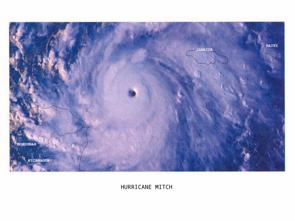
HURRICANE MITCH

A cross-sectional view of a hurricane showing the eye and eyewall of the storm system. Note the convergence of winds at the land’s surface and the divergence of winds aloft.

Mean structure of a mature hurricane (“Helene,” 26 Sept. 1958) in cross section, supposing axial symmetry. The left-hand half shows the boundaries of the eye-wall (solid lines, bending outward with height) and illustrates the cloud structure. The broken lines are contours of constant “equivalent potential temperature,” the absolute temperature in degrees Kelvin that the air would have with all of the latent heat in its vapor content released, and the pressure brought down to sea level pressure. In the right-hand half section, thin full lines are contours of constant wind speed in m s-1 (the thick lines repeat the eye wall boundaries), the broken lines are angular momentum contours, the dotted lines contours of temperature in °C. The maximum wind speed is in excess of 180 km/h. Note the stratiform cloud (dashed lines in the left half) extending to 13 km height, to the top of the troposphere, where the temperature is -55°C, = 218 K. Satellites see this “cloud-top” temperature. From Palmen and Newton (1969).

Global air circulation as described in the six-cell circulation model.

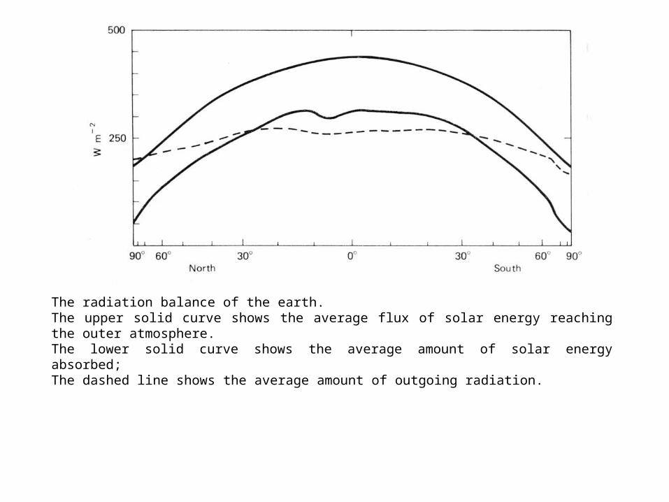
The radiation balance of the earth. The upper solid curve shows the average flux of solar energy reaching the outer atmosphere. The lower solid curve shows the average amount of solar energy absorbed; The dashed line shows the average amount of outgoing radiation.

Figure 7.10 Areas of heat gain and loss on earth’s surface. Since the area of heat gained (orange area) equals the area of heat lost (blue areas), Earth’s heat budget is balanced.

The radiative equilibrium solution (solid line) corresponding to the observed distribution of atmospheric absorbers at 35oN in April, the observed annual average insolation for the whole atmosphere, and no clouds. The dashed line shows the effect of convective adjustment to a constant lapse rate of 6.5 K km-1. In (a) the curves are drawn with a scale linear in pressure, i.e., equal intervals correspond to equal masses of atmosphere. In (b) the scale is linear in altitude. [From Manabe and Strickler (1964, Fig.4).]

The greenhouse effect. The glass is transparent to short-wave radiation, the net downward flux of which is I. The balancing upward flux of long-wave radiation from the ground is U, a fraction e of this being absorbed by the glass. This warms the glass, causing it to emit a flux B in both directions.

Radiation balance for the atmosphere. [Adapted from “Understanding Climatic Change,” U.S. National Academy of Sciences, Washington, D.C., 1975, p. 14, and used with permission.]

Streamlines of the mean meridional mass flux in the atmosphere for (a) December-February and (b) June-August. Units are megatons per seconds (Mt s-1 = 109 kg s-1). The horizontal scale is such that the spacing between latitudes is proportional to the area of the earth’s surface between them, i.e., is linear in the sine of the latitude.

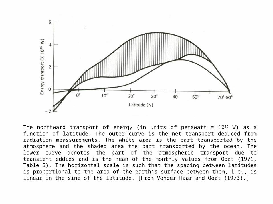
The northward transport of energy (in units of petawatt = 1015 W) as a function of latitude. The outer curve is the net transport deduced from radiation meassurements. The white area is the part transported by the atmosphere and the shaded area the part transported by the ocean. The lower curve denotes the part of the atmospheric transport due to transient eddies and is the mean of the monthly values from Oort (1971, Table 3). The horizontal scale is such that the spacing between latitudes is proportional to the area of the earth’s surface between them, i.e., is linear in the sine of the latitude. [From Vonder Haar and Oort (1973).]

Pathways of energy transfer in the global average energy budget. After Kiehl and Trenberth (1997)

Schematic of major features of the atmospheric circulation. The average circulation is idealized as being independent of longitude and symmetric about eh equator. The subpolar jet (dashed curves for upper-level features) is shown as a snapshot for a particular day that includes weather variations: an upper-level wave and an associated surface front. In a climate average, these features would not be present, yet they are important for maintaining climate. Along the right, the circulation in the vertical and in latitude is shown as a sequenc3e of overturning cells. The upper-level subtropical jet occurs near the poleward, descending branch of the Hadley cell. Circled crosses/dots represent flow into/out of the plane of paper

Major systems of ocean surface currents. Thick arrows denote stronger currents. Thinner arrows within gyre systems indicate weaker, widespread

flow.

Temperature as a function of height or pressure. Nomenclature for atmospheric vertical regions and common cloud types is also given. Temperature data are from the standard atmosphere except in the troposphere where it has been modified to a profile typical of deep convective regions. The vertical scale is linear in pressure from the surface to 100 mb, but stretched in the upper half

Precipitation climatology (July 1987 to July 1995) in mm per day. Estimated from a combination of satellite and ground rain-

gauge data (data from the Xie and Arkin (1996) date set)

Schematic diagram of the Walker circulation. Overturning cells along the equator in the east-west direction, with rising branches occurring in the convergence zones, associated with large amounts of convection. Note that the wind shown has the longitudinal average around the equator removed. Total wind tends to be predominantly easterly. Adapted from Madden and Julian (1972), and Webster (1983)

Sea surface temperature climatology for January and July (averaged 1982-2000). Note that the contour interval is smaller for warmer temperatures to show tropical features. Data are from the Reynolds et al. (2002) data set

Schematic of vertical temperature structure.