Air Traffic Control

A Air Traffic Control: An Overview Air traffic control (ATC) is a system whose basic objective is to provide safe and efficient flow of aircraft at airports and in the airspace. In clear weather with limited numbers of aircraft, individual pilots can see and avoid one another for safety and space themselves in queues for efficient flow of traffic. However, with high traffic density and in poor visibility, a system of centralized ground control is necessary to maintain safety and efficiency. This is the ATC system.

The major requirement is a means for surveillance of the traffic, but the system also requires communications, navigation facilities, weather information, rules and procedures. The form of ATC systems has varied greatly with time, traffic density, weather, technology and political conditions.

I . History of ATC in the USA Attempts to reach international agreement on general rules for air traffic started as early as 1910, but were unsuccessful until the International Commission for Air Navigation was developed at the Versailles peace conference in 1919. Although the USA failed to sign the treaty, it followed many of the concepts developed by the Commission. In 1929 the first air traffic controllers used checkered flags to clear aircraft for takeoff at busy airports. The first radio-equipped tower was opened at the Cleveland Municipal Airport in 1930. In 1935 the principal airlines opened three airway traffic control centers at Newark, Chicago and Cleveland. The government assumed responsibility for their operation in 1936 and rapidly expanded the number of centers.

These early centers used a teletype network for relaying information between airports and those ground stations with radio telephone facilities. By 1946, the number of centers had expanded to 24 and has stayed at about that level ever since. The jurisdiction of airport control towers was expanded to include control over aircraft making approaches under instrument conditions.

During the early 1950s, remote communications facilities were developed to provide direct pilot-to- controller communications. In the late 1950s primary radar was introduced, which allowed controllers to see aircraft positions in real time, albeit without altitude or identity information (which still had to be obtained by radio communication). Secondary radar was introduced in the 1960s. In the 1970s the secondary radar was upgraded to provide 4096 identity codes plus automatic altitude reporting. Computer data processing and computer-generated displays were also added to both the en route centers and the terminal approach facilities, which by now had been located remote from the airport control tower.

Upgrading of the data processing has continued with the addition of new features such as conflict alert, which provides the controller with a warning when it appears to the computer that two aircraft will come dangerously close together. Also, an improved form of secondary radar called mode S will soon be implemented. With this improvement will come two-way, digital, data-link communications.

The development of the ATC systen; in other countries has followed a similar pattern. Mode S, for example, has already received approval from the International Civil Aviation Organization (ICAO).

2 . Modes of Operation Four modes of ATC system operation are identified as a function of the surveillance capability available. These modes follow the historical development of ATC surveillance and are sometimes associated with the generations of ATC. The first mode was communications only. In this mode, the controller establishes the position and altitude of each aircraft from a pilot report. Traditionally, the information was recorded on strips of paper (one per aircraft) and stacked sequentially on a board which was updated by the controller. Aircraft were cleared in order down an airway or onto an approach path based on a report on his progress by the pilot ahead.

The second mode was primary surveillance radar (PSR). In this mode, the location of aircraft can be seen on the radar screen, but the controller has to identify the radar target and obtain altitude from pilot reports. Traditionally, the identity and altitude information is written on a small piece of plastic, which is pushed along by a controller to keep it close to its associated radar target. The piece of plastic is called a shrimp boat because of its characteristic shape. Because the controller can see the location of each aircraft, he can “vector” an individual aircraft along an arbitrary course by commanding heading and altitude assign- ments to the pilot over the communications radio channel. This technique is almost always the method used for merging and spacing of aircraft into and out of high-density terminal areas. Should the radar fail, the controller is obliged to revert to the communications only mode, relying on pilot reports to establish aircraft location.

The third mode was secondary surveillance radar (SSR). In this mode, identity and altitude information are automatically reported and available for computer processing. The display is computer generated, with a data block next to each aircraft symbol replacing the old shrimp boat. Data processing also provides velocity information, display options and many other features that make data readily available to the controller. The

1

Air Traffic Control: An Overview

transponder I--- - airborne ----- - and display

computer human pilot

surveillance sensor

screen no longer has to be horizontal (to support the shrimp boats). The computer also provides controller prompting when aircraft approach control boundaries, violate their altitude clearance or are threatened by other traffic. Should the SSR mode fail, the controller reverts to the PSR mode.

The fourth mode is mode S data link. In this mode, communications can be sent and received via the surveillance system. It will be possible to have messages generated automatically and data requested and transferred automatically between air and ground without the intervention of pilot or controller. In each of the first three modes, the actual control of traffic was always carried out by the human controller and transmitted by voice commands. With mode S it will be possible to effect control by the computer, with clear- ances issued automatically via the data link.

The four modes are compared in Fig. 1, where the flow of information is shown schematically. The upper boxes represent airborne components, and the lower boxes represent ground components. For mode S with data-link operation, information can flow in all the channels. With SSR, the dashed line is lost as a communications channel and the airborne display for data-link information does not exist. Although limited data can come down through the surveillance channel, all the data going up have to go directly through the voice radio link between controller and pilot. With the primary radar mode, the down link through the surveillance channel is lost and there is no computer- generated display of down-link information. In the communications only mode, the only elements remaining are the pilot and controller, who pass information by the voice radio link.

- ground computer - human --- &display - cant rol I er

3. Typical Flight Through the ATC System The actual separation of traffic within the ATC system has always been carried out by human controllers. The airspace is divided into sectors and within each sector one controller has legal responsibility for the separation of all flights which he has accepted within his sector. As a flight proceeds from one sector of airspace to another, this responsibility is handed from one controller to

another. The various controllers who handle a flight and their area of responsibility are as follows:

ground controller, responsible for airport surface traffic; tower controller, responsible for takeoff and landing traffic within 8 km of airport; departure controller, responsible for departing aircraft in transition to en route flight; center controller, responsible for en route traffic within a sector of the center; and approach controller, responsible for arriving aircraft in transition from en route flight.

The ground and tower controllers are located in the airport tower, where they have visual contact with the majority of traffic they control. The approach and departure controllers are usually located together with their surveillance displays near the prime airport in their terminal area. The center controllers are housed in a remote location somewhere within the geographic area they serve.

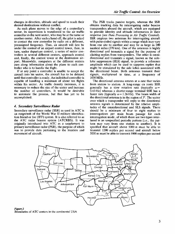
The boundaries of the US centers are shown in Fig. 2. The airspace of each center is subdivided into about 20 sectors. The sector controllers of a single center sit side by side within the center facility. They can effect a hand off by simply talking to one another. The coordination of a hand off between sector controllers in adjacent centers requires intracenter communication over land lines or through the computer system.

To understand how the elements work together, consider a typical airline flight. A flight plan which includes the route, destination, cruise altitude and characteristics of the aircraft is filed in advance and stored on the ATC computer. Before takeoff, a clearance is sent to the departure airport tower for relay to the flight. Departure may be delayed until the en route centers and the destination airport are ready to accept the flight. Once the flight has been cleared, it is handed off from controller to controller as it progresses. At each hand off, the pilot is given the radio frequency of the next controller who has assumed separation responsibility.

The location and altitude of the aircraft are picked up at regular intervals by beacon and radar. On the basis of such data, the computer presents moving points on each controller’s display screen that reflect the position and progress of each aircraft. Each point also carries information showing the identity, altitude and speed of each plane. In addition, the computer projects the path of each plane and gives visual as well as audible alarms if it expects two planes to come too close together. In general, alarms will be issued if lateral spacing becomes less than 8-16 km or vertical separation becomes less than lo00 ft (300 m), although these parameters vary with factors such as the altitude and speed of the aircraft. The controller advises the pilots of necessary

2

Air Trafjc Control: An Overview

changes in direction, altitude and speed to reach their desired destinations without conflict.

As each plane moves to the edge of a controller's sector, its supervision is transferred to the air traffic controller in the next sector, who may be at the same or another center. After such a hand off, the pilot is asked to contact the new controller by radio on a different, preassigned frequency. Thus, an aircraft will first be under the control of an airport control tower, then, in turn, under departure control, a series of sector controllers in several different centers, approach control and, finally, the control tower at the destination airport. Meanwhile, computers at the different centers pass along information about the plane to each controller who is to handle the flight.

If at any point a controller is unable to accept the aircraft into his sector, the aircraft has to be delayed until that controller is ready. An individual controller is capable of handling a maximum of about ten flights within his sector. As traffic density increases, it is necessary to reduce the size of the sector and increase the number of controllers. It would be desirable to automate the process, but that has yet to be accomplished.

4. Secondary Surveillance Radar Secondary surveillance radar (SSR) as used in ATC is an outgrowth of the World War I1 military identification friend or foe (IFF) system. It is also referred to as the ATC radar beacon system (ATCRBS). It was originally introduced into ATC as a supplement to primary surveillance radar (PSR), the purpose of which was to provide data pertaining to the location and movement of aircraft.

The PSR tracks passive targets, whereas the SSR obtains tracking data by interrogating radar beacon transponders aboard the aircraft, which are equipped to provide identity and altitude information in their response (see Data Processing in Air Traffic Control). SSR employs two antennas for interrogating aircraft with pulse-coded signals within a range which may vary from one site to another and may be as large as 200 nautical miles (370 km). One of the antennas is highly directional and transmits a signal for the purpose of eliciting replies from transponders. The other is omnidirectional and transmits a signal, known as the side- lobe suppression (SLS) signal, to provide a reference amplitude which can be used to suppress replies that might be stimulated by the side lobes associated with the directional beam. Both antennas transmit their signals, multiplexed in time, at a frequency of 1030 MHz.

The directional antenna rotates at a rate that varies from station to station. A long-range en route SSR generally has a slow rotation rate (typically w = 0.63 Hz) whereas a shorter-range terminal SSR has a faster rate (typically w = 1.26 Hz). The beam width of the directional antenna is in the region of 3". The sector over which a transponder will reply to the directional antenna signals is determined by the relative amplitudes of the omnidirectional and SLS signals. There should be a minimum of four to eight replies to interrogations per main beam passage for each interrogation mode, of which there are two types inter- laced in an unspecified periodic pattern (i.e., the pattern may vary from one station to another). It is specified that aircraft above 5000m must be able to transmit 1200 replies per second and aircraft below 5000 m must be able to transmit 1000 replies per second

n

Figure 2 Boundaries of ATC centers in the continental USA

3

Air Trafjc Control: An Overview

for a 15-pulse coded reply and, further, that the maximum interrogation frequency of any SSR shall be 450 interrogations per second.

Three pulses, designated in the sequential order of their transmission as PI , P2 and P3, form the interrogation signal. The first, PI, is transmitted by both antennas. The second, P2, is the control pulse transmitted only by the omnidirectional antenna. The third, P3, is transmitted only by the directional antenna.

The maximum power in the main beam of the directional antenna is recommended to be at least 24dB above that in the strongest side lobe, and the power of the signal transmitted by the omnidirectional antenna is supposed to be at least 9dB below the main beam maximum. Thus, an aircraft can determine whether it is receiving a main beam or a side-lobe signal by compar- ing the amplitudes of PI and P2. The transmission of PI by both antennas is intended to aid in discriminating against interrogation signals which are multipath reflec- tions from buildings or other structures rather than direct line-of-sight transmissions.

The time intervals between the PI and P3 pulses are of discrete lengths to designate any of six corresponding modes. Two of the modes are relevant to ATC: mode A (8 ps) requests identification and mode C (21 ps) requests altitude.

Reply signals are transmitted at a frequency of 1090 MHz in a format consisting of two framing pulses, designated as F, and F2 (see Data Processing in Air TrafJic Control).

The transmission time of a reply is determined by the range propagation delay of a valid P3 pulse; that is, one from a PI, P2, P3 reply sequence for which the relative pulse amplitudes are in a relationship appropriate to a main beam transmission. Thus, when the SSR interrogator receives the transponder reply delayed again by the range propagation, it can determine the range to the transponder from a measurement of the total time between the transmission of the P, pulse and reception of the first framing pulse in the reply (which it recog- nizes by the 2 0 . 3 ~ s interval between the FI and F2 pulses) after removing the fixed calibrated delays of the transponder. The SSR also estimates the azimuth of the transponder by beam splitting on all of the replies that have the same range delay.

Each SSR in a particular region transmits a different interrogation sequence pattern which can be used to identify it. The interrogation rate of any SSR is required to differ from that of any other by at least five interrogations per second. In addition, some transmit at a fixed pulse repetition interval (PRI), while others transmit in one of several possible staggered patterns.

5. Mode S The development of selectively addressed SSR (mode S) was started in the early 1970s in the UK under the name ADSEL (MacKellar and Evans 1979) and in the USA under the name discrete address beacon

Figure 3 SSR interrogation waveform with mode S all-call pulse added

systems (DABS) (Drouilhet 1974). After a letter of agreement was signed between controlling agencies in the two countries in 1974, the two systems were developed cooperatively using a common signalling format. The advantages of selective addressing are improved accuracy and performance, plus the provision for data transmissions as part of the interrogation and reply formats.

To support these improvements, it is necessary to reduce the number of interrogations, which requires that reliable position information be extracted from each reply. This involves the use of a monopulse bearing measurement which is similar to the technique used in tracking radars, namely, using sum and difference antenna patterns and the ratio of signal amplitude in each pattern to locate the aircraft precisely in azimuth. To provide conformity with existing SSSR equipment, mode S operates on the frequencies of 1030 MHz and 1090 MHz with a compatible signal waveform. This is achieved simply by adding a fourth pulse, Pa, 2.0 ps after the standard PI-P3 combination presently used in SSR, as shown in Fig. 3.

This particular waveform with the P4 pulse is defined as the all-call interrogation. It is used to interrogate all ATCRBS-equipped aircraft and for initial acquisition of the addresses of all mode S equipped aircraft for storage in a roll-call file. The SSR transponders recognize the first three conventional pulses, PI , P2 and P3, but ignore the P4 pulse, whereas Mode S transponders recognize the presence of P4 as a request for discrete address. If there is no P4 pulse present, as from an SSR interrogation, the mode S transponder replies in the conventional SSR mode. Once the ground sensor has acquired a mode S aircraft on roll call, the transponder is locked out from future all-calls, except under well- defined operational rules, and replies only when speci- fically addressed with its unique 24-bit discrete address code.

The discrete interrogation, as distinct from the all- call interrogation, is accomplished by again taking advantage of the SSR waveform. If an SSR transponder receives a P2 pulse 2 PS after receiving the first pulse at the same relative amplitude or within 9 dB, it automatically suppresses and will not reply. Mode S uses this scheme to cause SSR transponders to suppress while

4

Air Traffic Control: An Overview .

interrogating on mode S. This is accomplished by radiating PI and P2 in the main beam at the same amplitude. Mode S transponders recognize the PI-P2 combination as a discrete interrogation and wait 2 ps for the data block that follows. The data block contains either a 56-bit surveillance-only interrogation asking for the altitude of the aircraft, or a combination of surveillance and a 56-bit general data link message-a total of 112 bits.

There is also a third format that replaces both the 56- bit surveillance and the 56-bit data combination with an 80-bit data-only message. This latter format is used when long transmissions of data are required and is termed the extended length message (ELM). Up to 16 ELM segments can be transmitted sequentially to any suitably equipped aircraft while it is in the main beam, requiring only a single reply to acknowledge receipt. This allows large quantities of data to be transferred without excessive replies.

The modulation used for the uplink data block is differential phase shift keying (DPSK); a phase shift of 180” during a 0.25 ps bit space represents a binary 1; no phase shift in the bit space is 0.

The mode S reply format uses a pair of double pulses as a preamble to the data block containing either the 56-bit surveillance-only reply or the combination of 112-bit surveillance and data message or ELM reply. The modulation used on the downlink is pulse position modulation (PPM), where the position of the pulse determines whether it is a binary 1 or 0. The bit rate for all uplink formats is four megabits per second and one megabit per second for the downlink.

Mode S provides a position accuracy about six times as good as that of SSR, plus a reliable digital data link. Implementation is expected to have taken place by the early 1990s.

6. Backup Assurance While the ground-based ATC system as described above is intended to prevent conflicts between aircraft, there are many instances when, for one reason or another, two aircraft fail to maintain separation. Research has been continuing since the mid-1960s to develop an airborne collision avoidance system (CAS) which would provide a backup to the primary ground- based ATC system when two aircraft, for whatever reason, find themselves on a near collision course with only just enough time remaining to make an escape maneuver (Bulford 1972, 1978) (see Airborne Collision Auoidance). The traffic alert and collision avoidance system (TCAS) is an outgrowth of the 20 years of CAS development and shows considerable promise for near- term implementation. TCAS is built around the mode S transponder.

The mode S transponder performs the same basic functions as the mode C transponder; that is, it automatically transmits aircraft identity and altitude data when triggered from the ground or the air. The principal

advantage of the mode S transponder is its discrete, or selective, address capability. This selective address capability results from the fact that signalling formats which provide more than 16 million available codes are utilized, compared with 4096 for mode C equipment. This means that each mode S unit can be assigned a permanent call number.

In use, the mode S transponder transmits a periodic “squitter” signal which informs all TCAS-equipped aircraft in the area of its identity. This identification process establishes data-link communications for relaying TCAS advisories and collision avoidance information.

TCAS represents a development of the beacon collision avoidance system (BCAS) (Welch and Orlando 1980). The major technical improvement is the use of a directional antenna that permits reliable operation in high-density terminal areas. Like BCAS, TCAS determines the position of other aircraft in the vicinity by interrogating their transponders and analyzing the replies. It then presents appropriate traffic advisories and conflict resolution advisories to the pilot on his cockpit display.

In addition, TCAS will generate collision avoidance advisories for all conflicts involving aircraft with SSR altitude-reporting transponders. Initially, the equipment will provide only vertical escape maneuvers and the pilots will be advised either to descend or to climb. Horizontal maneuvers are a possibility for later versions. Moreover, when two TCAS aircraft are in conflict, the avoidance maneuvers will be coordinated via the mode S data link.

TCAS also communicates its position and intended collision avoidance maneuvers to mode S equipped airplanes using the crosslink feature. Proximate aircraft can be displayed on a VDU relative to the position of the receiving aircraft. Resolution advisories are typically generated with only 30s remaining until closest approach.

Another approach to backup assurance is a cockpit display of traffic information (CDTI). CDTI differs from TCAS primarily in the longer range over which the CDTI display shows proximate aircraft. CDTI would also show a map background on the display so that the pilot could monitor the ATC operation as it applied to traffic in his vicinity. Although there has also been considerable research on CDTI (Connelly 1975), it is expected that TCAS will be implemented first.

Bibliography Alexander B 1969 Air Trafjic Control Advisory Committee

Report. US Government Printing Office, Washington, DC

Bulford D E 1972 Collision avoidance: An annotated bibliography, FAA-NA-72-41. Federal Aviation Administration, Washington, DC

Bulford D E 1978 Collision avoidance: An annotated bibliography, FAA-NA-78-8. Federal Aviation Adrnin- istration, Washington, DC

5

Air Traffic Control: An Overview

Connelly M E 1975 Applications of the airborne traffic situation display in ATC. A G A R D Conf. Proc., Vol. 188. Advisory Group for Aerospace Research and Development, Neuilly-sur-Seine, France

Drouilhet P R 1974 Provisional signal formats for the discrete address beacon system, MIT Lincoln Laboratory ATC-30, FAA-RD-74-62. Federal Aviation Administration, Washington, DC

Gilbert G A 1973 Air Traffic Control: The Uncrowded Sky. Smithsonian Institution Press, Washington, DC

Karp S, Haroules G G, Klein L (eds.) 1973 Special is- sue on aeronautical communications. IEEE Trans. Commun. 21(5)

Kayton M, Fried W R 1969 Avionics Navigation Systems. Wiley, New York

MacKellar A C, Evans A J 1979 ADSEL-An improved form of secondary surveillance radar. ICAO Bull. 34(3)

Orlando V A, Drouilhet P R 1980 DABS: Functional description, MIT Lincoln Laboratory ATC-42A, FAA-RD-80-41. Federal Aviation Administration, Washington, DC

Welch, J D, Orlando V A 1980 Active beacon collision avoidance system (BCAS), MIT Lincoln Laboratory ATC-102, FAA-RD-80-127. Federal Aviation Admin- istration, Washington, DC

W. M. Hollister [Massachusetts Institute of Technology,

Cambridge, Massachusetts, USA]

Air Traffic Control Near Airports The increase in the volume of air traffic since the mid-1970s has led to a congestion of the air space, particularly in airport areas. This condition leads to interrupted climbs and descents, wasted time, and increases in both delay and fuel burnt resulting in increases in both operating costs and work load for pilots and control services. In turn, this means possible adverse consequences for safety. Such a situation will worsen in the future since an increase of 5% per year of total flights controlled seems to be realistic in spite of the so-called energy crisis (see Flight Activity: Prevision).

Short-term control in an airport area is exercised basically through area navigation. This allows good use of runway capacity while ensuring the desired separation between aircraft. However, this does not guaran- tee a satisfactory decrease in fuel consumption and delays because of the brevity of the control time span, the necessity to modify the ground track (i.e., the ground projection of the flight path), the low altitude and, consequently, the high-fuel-consumption flight evolutions and holding patterns. Hence, the need to optimize the use of available system capacity leads to the consideration of an extended zone of control.

Such an extended zone of control, combined with an accurate prediction of future flight paths, should allow aircraft to approach the runway on uninterrupted descents at idle thrust (leading to a reduction in fuel consumption) and along given ground tracks (giving a

controller workload reduction). By considering the flux of aircraft entering the system, it should then be possible to ensure a “global” optimization of the traffic.

1. Analysis of the Problem Before considering the control problem itself, a global analysis should be made of the objectives and constraints. The system constituted by air traffic management in a zone of convergence is particularly complex due to the variety of objectives that must be satisfied, the number of constraints inherent in the system, the variety of functions to be performed (e.g., management, sequencing, scheduling, conflict detection and resolution) and the modelling problems associated with variations in aircraft performances.

Broadly, the problem is to guide to the runway a flow of aircraft which enter the zone in a quasirandom fashion with respect to altitudes, speeds and arrival times.

In addition to constraints related to individual operating conditions of aircraft and to the constraints regarding procedures, an air traffic control (ATC) system must satisfy the safety standards which lay down a minimum separation between any two planes at any instant.

The overall objective is to minimize the global transit cost for all aircraft in the system. This global cost reflects the capability of the system to reduce both delays (i.e., indirect operating costs) and total consumption of fuel. The two objectives of minimization of transit time and of consumption are somewhat conflict- ing; minimum transit time for an individual aircraft requires the aircraft to proceed at the maximum allow- able speed. Such a procedure may decrease some of the indirect operation costs, but at the expense of a signifi- cant increase in the fuel consumption. Alternatively, the minimum fuel trajectory requires the aircraft to descend at low speed. In practice, some compromise between these two policies is looked for by airlines, by weighting time spent and fuel burnt. The corresponding strategy may vary from one company to another and may be summarized by the definition of a “preferred profile” for each type of aircraft (see Fuel Conservation: Air Transport).

If the total cost of transit for all aircraft in the zone from a global point of view is considered, with the same criteria, the solution can be analyzed as a compromise between (a) the minimization of the sum of the delays encoun-

tered by all the aircraft (a delay is the difference between the transit time actually experienced by an aircraft from its entry into the zone to landing and the nominal time it would have spent if alone in the zone and descending on its preferred profile); and

(b) the minimization of the global quantity of fuel burnt by all aircraft (it is important to note that the

6

Air Traffic Control Near Airports

fuel consumption is dependent not only on time spent, thrust and speed, but also on altitude and, thus, for a given delay, fuel consumption depends on whether the delay occurs in level flight or in idle-thrust descent in the case of a level tracking on its altitude).

Any control procedure aimed at minimizing cost and/or fuel consumption will be efficient (i.e., will bring appreciable savings) only if the extent of the zone is sufficiently large. For this reason, the zone of control considered in this article, called the zone of convergence, is larger than the current airport area; for practical purposes, the radius of this zone varies from 100 nautical miles (185 km) to 200 nautical miles (370km) around the airport of interest. In western Europe, a 100 nautical mile zone could be implemented on a national level. A 200 nautical mile zone implies international cooperation, in some cases, but its potential savings will be appreciably higher.

2 . Dynamic Scheduling The scheduling technique is essentially based on landing sequencing and on control of cruise and descent speed profiles. The landing sequence and the descent profiles have to be chosen in order to minimize the predefined criterion (i.e., the total transit cost for all aircraft from their entry into the zone to touchdown).

One of the difficulties associated with scheduling lies in its dynamic nature: each time an aircraft enters the zone a new optimal sequence has to be computed for the aircraft in the zone. This requires the design of an efficient optimization technique compatible with real- time operation.

There are two basic ideas underlying scheduling policy. First, it may be possible to improve the landing sequence since the minimum time separations between two landing aircraft depend on the types of plane involved. Second, it is possible to control the descent speed of aircraft, in order to improve the traffic flow: a fast descent may decrease the waiting time of following aircraft and a slow descent allows delays to be absorbed with reduced consumption, the waiting time being spent at idle thrust.

2.1 Sequencing Constraints The safety standards at the runway or, more specifi- cally, on the last common track of the instrument landing system (ILS) are defined in terms of longitudinal separation. This separation s,(i, j ) between two aircraft, the jth aircraft following the ith aircraft, depends on the couple considered, since vortex pheno- mena imply a greater separation behind a jumbo jet than behind a medium-haul aircraft. To this longitudinal separation in nautical miles corresponds a time separation for landing s ( i , j ) . This depends on the longitudinal separation, the length of the last common track and the speeds of the two planes. The range of

entry 7 new Mach number

\ eventual holding

dexent COnstant with CAS

runway

Figure I Classical aircraft descent procedure

speeds and the differences in length of the last common track of the routes lead to an important range of separations. The ratio between extreme values may reach a value of three. Because of this range of separations, optimization of the landing sequence may be efficient and improve the runway occupancy, thereby reducing potential delays.

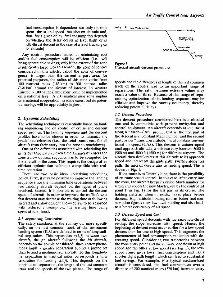
2.2 Descent Procedure The descent procedure considered here is a classical one and is compatible with present navigation and control equipment. An aircraft descends at idle thrust along a “Mach-CAS” profile; that is, the first part of the descent is at constant Mach number and the second part, below “transition altitude,” is at constant conventional air speed (CAS). This descent is uninterrupted until approach altitude, which can vary between 3000 ft (900 m) and 5000 ft (1500 m) for different airports. The aircraft then decelerates at this altitude to its approach speed and intercepts the glide path. Further along this path, the aircraft decelerates to landing speed. This is shown in Fig. 1.

If the route is sufficiently long there is the possibility of en route speed control. In this case, after entry into the zone, the aircraft keeps its cruise Mach number for 4 min and adopts the new Mach given by the control (at point P in Fig. 1) for the last part of its cruise. The holding pattern, when it exists, takes place before descent. High-altitude holding returns better fuel consumption figures than low-level holding and also leads to a better occupancy of air space.

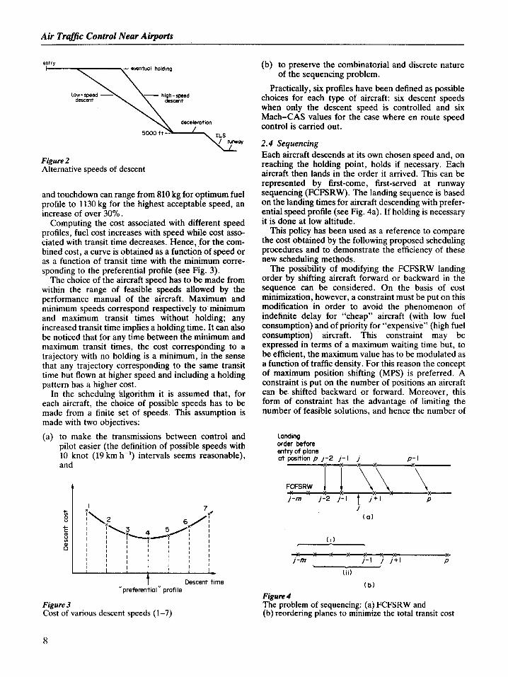
2.3 Descent Speed and Cost For different speed descents with the same idle-thrust setting, the slope increases with speed. Hence, the beginning of descent must occur earlier for a low-speed descent than for one at high speed. This augments the phenomenon of fuel consumption reduction with decreasing speed. Considering two trajectories between the zone entry point and the runway, one flown at high speed and the other at low speed (see Fig. 2), the low- speed cruise gives lower fuel consumption and has a shorter flight path length, which can lead to substantial fuel savings. For example, if a typical medium-haul aircraft is considered, the fuel consumption over a distance of 200 nautical miles (370 km) between entry

7

Air Trafjc Control Near Airports

deceleration

high-speed descent descant

A-Rww deceleration

Figure 2 Alternative speeds of descent

and touchdown can range from 810 kg for optimum fuel profile to 1130 kg for the highest acceptable speed, an increase of over 30%.

Computing the cost associated with different speed profiles, fuel cost increases with speed while cost associated with transit time decreases. Hence, for the combined cost, a curve is obtained as a function of speed or as a function of transit time with the minimum corresponding to the preferential profile (see Fig. 3).

The choice of the aircraft speed has to be made from within the range of feasible speeds allowed by the performance manual of the aircraft. Maximum and minimum speeds correspond respectively to minimum and maximum transit times without holding; any increased transit time implies a holding time. It can also be noticed that for any time between the minimum and maximum transit times, the cost corresponding to a trajectory with no holding is a minimum, in the sense that any trajectory corresponding to the same transit time but flown at higher speed and including a holding pattern has a higher cost.

In the schedulng klgorithm it is assumed that, for each aircraft, the choice of possible speeds has to be made from a finite set of speeds. This assumption is made with two objectives:

(a) to make the transmissions between control and pilot easier (the definition of possible speeds with 10 knot (19 km h-I) intervals seems reasonable), and

t

t Descent time ”preferential” profile

Figure 3 Cost of various descent speeds (1-7)

(b) to preserve the combinatorial and discrete nature

Practically, six profiles have been defined as possible choices for each type of aircraft: six descent speeds when only the descent speed is controlled and six Mach-CAS values for the case where en route speed control is carried out.

2.4 Sequencing Each aircraft descends at its own chosen speed and, on reaching the holding point, holds if necessary. Each aircraft then lands in the order it arrived. This can be represented by first-come, first-served at runway sequencing (FCFSRW). The landing sequence is based on the landing times for aircraft descending with preferential speed profile (see Fig. 4a). If holding is necessary it is done at low altitude.

This policy has been used as a reference to compare the cost obtained by the following proposed scheduling procedures and to demonstrate the efficiency of these new scheduling methods.

The possibility of modifying the FCFSRW landing order by shifting aircraft forward or backward in the sequence can be considered. On the basis of cost minimization, however, a constraint must be put on this modification in order to avoid the phenomenon of indefinite delay for “cheap” aircraft (with low fuel consumption) and of priority for “expensive” (high fuel consumption) aircraft. This constraint may be expressed in terms of a maximum waiting time but, to be efficient, the maximum value has to be modulated as a function of traffic density. For this reason the concept of maximum position shifting (MPS) is preferred. A constraint is put on the number of positions an aircraft can be shifted backward or forward. Moreover, this form of constraint has the advantage of limiting the number of feasible solutions, and hence the number of

of the sequencing problem.

landing order before entry of plane at position p j - 2 j - l J P- I

..-Y-x-x..

FCFSRW ---x--x- J-m 1-2 j -1 t j + l P

)(. y x - X - Y - x J -m J - I j j + l P

( i i )

( b )

Figure 4 The problem of sequencing: (a) FCFSRW and (b) reordering planes to minimize the total transit cost

8

Air Traffic Control Near Airports

solutions to explore, and the solution can be found in real time.

The value of the MPS parameter is chosen to be an integer between one and four. An MPS equal to four means that an aircraft that occupies position n in an FCFSRW sequence may occupy positions n - 4 to n + 4 in the new schedule.

2.5 Optimization Each time a new aircraft enters the zone, the problem of finding the “best” landing sequence and the “best” descent profiles to minimize a generalized cost criterion must be solved.

This optimization applies to all aircraft in the zone that have not initiated descent; that is, lmin before descent (or holding when it exists), the highest point of the descent profile is given to the aircraft and cannot be subsequently changed. In the case where en route speed control is applied, the cruise and descent speed profile is fixed 1 min before cruise Mach-number change (i.e., 3 min after zone entry), but the landing time may be changed throughout the holding pattern until 1 min before holding (or descent).

When the pth aircraft enters the zone its landing number in the FCFSRW order can be determined on the basis of its potential landing time on the preferential profile descent with no delay. Thus, an optimal permutation of landing order under the constraint of maximum position shifting for all aircraft must be found. If the FCFSRW order of the entering aircraft is j and the maximum position shift is m, the possible positions for this plane are given by the increasing sequence of integers beginning with j - m and ending with j , so that scheduling for all aircraft from j - m - 1 to j must be considered. This optimization is achieved in several steps (see Fig. 4b): (a) Determine the sequence of the m + 1 aircraft pre-

ceding j , with j landing last, and determine the profiles for those aircraft (there being n possibilities for each), including aircraft j , in order to minimize their total transit cost (see (i) in Fig. 4b).

(b) On the basis of the new sequence, repeat the preceding scheme considering the m + 1 aircraft preceding j + 1, with aircraft j + 1 landing last (see (ii) in Fig. 4b).

(c) Repeat until aircraft p is the last to land. So, at each of the p - j + 1 steps of this optimization, the algorithm has to select one among ( m + l)! permutations of aircraft and, for each of the m + 2 aircraft, it has to select one among the n possible descent profiles that can be assigned to an aircraft.

The objective is to minimize the total transit cost (time plus fuel) under the constraint of the landing separations, which are given in the form of a time- separation matrix, The number of possibilities is (m+ l)!n”+* at each of the p - j + 1 steps. With six possible profiles ( n = 6 ) and a maximum value of

position-shifting parameter m of four, the number of possibilities is approximately 5.6 million. Of course, if one of the aircraft concerned has attained the point after which it cannot be reordered, the optimization applies to the subsequent aircraft only and the number of cases is reduced.

An optimization program suitable for solving this problem within the computing-time constraints compatible with real-time use has been developed. The branch-and-bound algorithm is used. This essentially consists of separating the set of solutions into subsets for which the evaluation of a lower bound of the criterion is possible and exploring at each step the branch with minimum lower bound. The efficiency of such an algorithm depends mainly on the quality of both the separation principle and the evaluation of the lower bound for the criterion. In the present case, the algorithm performances are most satisfactory and lead to an average computing time of 0.5s on a typical minicomputer to obtain the optimum solution each time a new aircraft enters the system.

The derivation of optimality and constraints equations, as well as details concerning the branch-and- bound resolution algorithm, are given in Sect. 5.

3. Operational Considerations and Constraints 3. I Control-Pilot Communication The scheduling program is run every time a new aircraft enters the zone. The transmission of the type of aircraft, its weight, flight level and speed allows the optimization program to select a landing sequence and a speed for all aircraft still cruising in the zone. The schedule is recomputed at each new entry, but the controller has to communicate the result to each aircraft only once; in fact, the controller transmits descent parameters to an aircraft only when these are firmly decided and the aircraft cannot be reordered any more (i.e. 1 min before descent or eventual holding). The parameters to be transmitted are holding duration, top of descent (i.e., the point where the descent has to be initiated) and speed of descent.

It has been deliberately supposed that transmissions take place without a data link; this is unnecessary since the small number of parameters to be transmitted will not significantly increase the workload for both pilot and control.

3.2 Aircraft Separation and Conflict Resolution In the sequencing process, the separation constraint between aircraft is taken into account only for the approach and landing phases, and takes the form of the time-separation matrix. It ensures standard separation of all aircraft between the end of their descent and the runway.

When the optimization is performed, the speed profiles for the aircraft and their times of landing are known, and their trajectories can be predicted: it is

9

Air TrafJic Control Near Airports

then necessary to verify that they are nonconflicting. A conflict prediction algorithm is implemented and the solutions proposed for any resolution are based either on flight-level change or earlier descent. The associated speeds are, in all cases, computed so that the aircraft land at the scheduled time and the landing order remains unchanged.

3.3 Trajectory Prediction and Tracking Precision (a) Prediction and aircraft modelling. The sequencing algorithm uses, as the data for each aircraft, the predicted time of landing and the cost (i.e., predicted consumption) associated with all possible predefined speed profiles. These data must be available for computation very shortly after the entry of an aircraft into the zone-as soon as its type, flight level, cruise Mach number and weight are known.

Generally, models of aircraft that include aerody- namics and propulsion characteristics are well known as the flight mechanics equations but, to meet the require- ments of computation time, it is not feasible to inte- grate this model on-line. Therefore, the model used should be of some “aggregate” form. The kind of representation used can be precomputed times and consumptions for each type of aircraft, and can be for different entry levels, aircraft weights and winds. The method used here is the representation proposed by Benoit and Swierstra (1981) in the form of polynomial approximations of time, distance for descent and fuel consumption as functions of speed, given for different weights and flight levels. The meteorological conditions (pressure, temperature and, most importantly, winds) must also be introduced.

The accuracy of such polynomial approximations is sufficient for the scheduling purpose, but the main difficulty lies in wind prediction. Several experiments have been conducted to try to evaluate the error on final time between a precomputed trajectory and a real trajectory (Imbert et al. 1976, Pelegrin and lmbert 1977). All experiments have indicated that the error is due mainly to the poor accuracy of wind conditions prediction and, especially, of altitude wind profile prediction.

The results show that the errors in the final arrival times are too large to be consistent with an efficient scheduling strategy. If the separation times taken into account for the scheduling must include the uncertainty in arrival times, the runway capacity decreases considerably.

If the efficiency of the scheduling algorithm relies heavily on the capability to predict an aircraft trajectory, the problem can be reversed and it can be considered as relying on the capability of an aircraft to fly a predefined trajectory and reach the runway at a prescribed time, with or without control intervention. In order to ensure the final-time accuracy, the scheduling function must then be associated with some trajectory tracking algorithm.

(b) Trajectory tracking. It is clear that the accuracy of trajectory tracking relies on the technological aids available, either for trajectory data transmission or for actual tracking.

The feasibility of four-dimensional control of the actual position of the aircraft with respect to the desired position can be envisaged in the near future. This assumes the capability to accurately measure the position of an aircraft and the generation of the corresponding control commands. This function could be ensured by onboard computers of flight management system (FMS) type which have been developed by several avionics manufacturers.

A less sophisticated solution, compatible with current technology or in the future with small-aircraft equipment, relies on speed and heading corrections along the descent trajectory (Imbert et al. 1976. Pelegrin and Imbert 1977). Taking into account the control load and the pilot task, the number of corrections has been limited to three: two speed adjustments during level flight and descent, and a heading correction before ILS interception. The correction magnitude is computed on the ground on the basis of the recorded errors between theoretical and actual positions of aircraft, and the new value of speed or heading is transmitted to the pilot by the standard present transmission means.

The proposed solution has been tested in simulation and in the real environment on commercial flights. The error in final arrival time, which could be 1 min in the worst cases without any correction, can be reduced to the order of 10 s with correction.

4. Example of Results Different samples of traffic on different real extended terminal areas have been checked in simulation in order to investigate the potential benefits of the proposed type of control.

A traffic sample is characterized by the distribution between different aircraft classes and by its density: the traffic density may be defined with reference to the runway capacity, which corresponds to the average number of aircraft that may land on the runway per hour. Since the time separations depend on the aircraft types, the capacity is a function of distribution and of the separation matrix. An average runway capacity is about 36 aircraft per hour. The traffic density is defined as a percentage of the runway capacity.

The samples for which the results are presented in this article include nine types of aircraft, ranging from a twin-engine light transport aircraft (Aerospatiale N 262) to wide-bodied long-range aircraft (McDonnell Douglas DClO and Boeing 747).

Figure 5 shows the results obtained for different samples: they have been generated by considering the same sequence arriving at zone entry gates at a rate ranging from 60% to 125% of the runway capacity. The

10

Air Trafjc Control Near Airports

l o o o r

v) 900 23 4 -

8 6001

I I I I I I I I 60 70 80 90 loo I10 120 I30

Traffic density of entry (% of runway capacity) - FCFSRW

,+--a cruise speed control with MPSz4 o......~ minimum cost per aircraft

Figure 5 Comparison of costs of landing using different control procedures in the mid-1 980s

zone considered was a fictitious zone with twelve entry gates located 200 nautical miles (370km) from the runway and convergence points located at 100 nautical miles (185 km) and 60 nautical miles (110 km) from the runway. The average total transit cost was plotted from entry to landing for different policies: the FCFSRW procedure and optimization with cruise speed control and maximum position shifting parameter equal to four. The reference is the average minimum transit cost per aircraft, that is, the transit cost on preferential profile with no delay. This minimum may certainly not be achieved for saturated or oversaturated traffic; however, this value has been adopted in the absence of any measure of the reachable minimum.

The FCFSRW procedure can be considered as an approximation of the current practice. Nevertheless, it is clear that this procedure and the assumptions underlying it (i.e. uninterrupted descent and generalized use of preferential profiles in particular) constitute an opti- mistic view of the real situation as far as overall transit costs and fuel conservation procedures are concerned. This obviously implies that the system efficiency is somewhat underevaluated.

From these results and all the results obtained for different traffic samples and different zones (Imbert and Comes 1978, Imbert et al. 1979, Imbert 1980, 1982), some conclusions concerning the benefits expected from dynamic scheduling may be deduced. First, as already noted, the computing time is certainly compatible with real-time implementation, with an average of 0.5 s for each new computation. Second, an obvious conclusion is that the optimization is more effective in saturated conditions of traffic, since there is

no major problem of waiting time for traffic density under 80%. Third, efficiency is increased only for a sufficiently large zone. The sequencing algorithm is applied when an aircraft enters the zone to all aircraft still in cruise. If the length of the routes is too small, aircraft are in descent when entering the zone or begin their descent very soon after this so that the number of aircraft in cruise is not sufficient for efficient sequencing. Fourth, the length of the different routes also have to be “homogeneous.” A zone with very long and very short routes may lead to a kind of “locking” of the system. If an aircraft arrives in the zone very shortly before landing, it is not possible to reorder the other aircraft that are already descending and the new plane has to wait. In this case, the result of dynamic scheduling, with its hypothesis of uninterrupted descents, can be worse than the result of present policy.

5. Mathematical Treatment When the pth aircraft enters the zone, if its FCFSRW number is j , the following problem must be solved p - j + 1 times: find the sequence and the speed profiles of N aircraft, and the speed profile of the (N+l) th that minimize the total transit cost, under the runway separation constraint.

The criterion for these N + 1 aircraft is

N+ 1

where i refers to the present order of the N + 1 aircraft, ti is the transit time in the zone from entry to runway including eventual holding time, ai is the cost per unit time (fuel excluded) for the ith aircraft, Ci is the total fuel consumption of the ith aircraft in the zone and Pi is the unit fuel rost (see Fuel Conservation: Air Transport).

The criterion may be separated into two parts, one corresponding to transit itself, the other to the eventual holding pattern. Defining t:k as the transit time of the ith aircraft on the kth speed profile (1SkSkmaX) , cik as the corresponding consumption, t: as the holding time and d i as the holding fuel consumption per unit time, then

c = c a i ( t ‘ i k + f h j ) + B i ( C j k + ~ i f : )

I

where C,k is the total transit cost on kth profile and y, is the total holding cost per unit time.

11

Air TrajJ'ic Control Near Airports

The problem is to find the landing position j and the speed profile for each aircraft i. Define

y j , k : l < i < N , 1 < j < N , 1<k<kmax

where y . . =1 qk 7

and

Note that

iff aircraft i lands in the jth position and descends with kth profile, where the permutations (ijk) satisfying this condition are to be provided,

y j j k = O in all other cases

c Y i j k = rk

In addition, define

Z k : l S k S k m a x

where

z k = 1 iff aircraft ( N + 1) descends with kth profile

and

z k = 0 otherwise

Note that

In the following, the subscript i will correspond to a particular aircraft and the subscript j will correspond to a landing position. The separation constraints are easier to write if the holding time is defined corresponding to a landing position, rather than to a particular aircraft.

Let t: be the holding time of aircraft landing in the jth position where

l S j S N + l (8 )

and let to be the initial time (i.e., the instant when the previous aircraft has landed), So, the separation time between this aircraft and aircraft i, S,, the separation time between aircraft i and I, Sd the separation time

between aircraft i and N + 1, and t j k the possible time of arrival at the runway of aircraft i descending on profile k (with no holding). With these definitions, the landing time of an aircraft in the jth position is

(9) ik

and the separation time between aircraft landing in positions j and j + 1 is

c Y i j k Y l ( j + I )k fS i / ilkk'

So, the N + 1 separation constraints may be expressed as

ik ilkk' lk'

ik ik k

The problem is then to find the y j j k and the Z k minimizing C under the constraints in Eqn. (11).

The resolution is a branch-and-bound technique; the principle is to branch the set of solutions into subsets, with an evaluation at each separation of a lower bound of the criterion. In this case, the separation is based on the allocation of a landing position to an aircraft and on the choice of a particular profile.

ALGORITHM Step 1: The solutions are separated into N subsets,

subset i corresponding to aircraft i in the first position.

Step 2: Each of those subsets is separated on the basis of all possible profiles for this first aircraft.

Step 3: The subset of solutions, with aircraft i with the kth profile landing in the first position, is divided into subsets corresponding to plane 1 in the second position (I # i ) .

This repeats until the profile of the (N+ 1)th aircraft. The tree generated for the case where N = 5 and with

six possible speeds per aircraft has about 5 x lo6 nodes. Some of these can be eliminated by considering MPS constraint or criterion properties. At each node of

12

Air Traffic Control: Trends

the tree, a lower bound of the criterion must be evaluated for all solutions of the subset it represents. The criterion may be written as

In the first term, if the profile of aircraft i is not chosen at the considered node, the minimum cost for this aircraft is taken (preferential profile).

For the second term representing waiting-time cost, a lower bound of the waiting time has to be evaluated for nonassigned positions. To evaluate a lower bound of the waiting time of an aircraft in the jth position the first inequality is used where it appears:

ik

The quantities in the first term are replaced by their minimum value, the additional quantity of the second term is replaced by its maximum value.

The waiting times or their lower bound correspond to a position and not to an aircraft, but the waiting-time costs are known per aircraft; a lower bound of the total waiting cost is obtained by multiplying the waiting times (in order of decreasing values) by the costs (in order of increasing values).

Hence, at each node, a lower bound of the criterion may be evaluated for all the solutions it includes. This value has to be compared with all node evaluations already achieved and the algorithm starts from the node with the lowest value.

The convergence properties of the algorithm are related to the quality of evaluation and separation. The computing time and the core occupancy depend on the number of explored nodes; at each step it is necessary to store the extreme nodes with the corresponding value of the criterion.

The convergence of the algorithm with the predefined separation and evaluation techniques are most satisfactory and lead to the possibility of real-time implementation.

6. Scheduling for Several Airports Practical results have pointed out the potential benefits of dynamic scheduling of traffic in a convergence zone. The principle is that with an enlargement of the zone it is possible to use the speed as control variable in order to improve the traffic flow and optimize the landing sequence.

An extension of this principle is coordination between several airports. Good as the sequencing

algorithm may be, it has to deal with randomly entering aircraft. Taking into account the trajectory of aircraft further “upstream,” it is possible to take their departure time as a control variable and to have them wait before taking off rather than hold before landing.

The problem for a set of airports is then to find a takeoff and landing sequence for each of them, in order to minimize a global cost criterion for the transit of all aircraft. The high coupling between airports and the existence of “external” traffic (i.e., aircraft with out- side airports as origin or destination) lead to a highly complex optimization problem. If, theoretically, the same algorithms can be used for this problem, the computing-time constraints require the use of parallel computing and of suboptimal solutions. The results obtained so far show the feasibility and the benefits of such a solution. See also: Airborne Collision Avoidance

Bibliogmphy Benoit A, Swierstra S 1981 Simulation of air traffic control

operation in a zone of convergence-aircraft performance data. Rapport Eurocontrol Doc. 812031-2

Imbert N 1980 Application de l’algorithme d‘ordonnancement du trafic a6rien h la zone de Londres Heathrow. Rapport CER T- D ERA 117240

Imbert N 1982 Algorithme de detection et de resolution de conflits entre trajectoires d’avion. Rapport

Imbert N, Comes M 1978 Gestion stratkgique de trafic en zone de convergence ordonnancement dynamique et r6sultats. Rapport CERT-DERA 6-7/7172

Imbert N, Filleau J B, Fossard A 1976 Etude de la pr6cision de navigation en zone terminale. Rapport

Imbert N, Fossard A J, Comes M 1979 Gestion ?i moyen terme du trafic a6rien en zone de convergence. Proc. IFACIIFORS Symp. Comparison of Automatic Control and Operational Research Techniques Applied to Large Systems Analysis and Control. pp. 155-62

Pelegrin M, Imbert N 1977 Accurate timing in landings through air traffic control. AGARD Conf. Proc. 24. North Atlantic Treaty Organization, Neuilly-sur-Seine, France

CERT-DERA 217240-02

CERT-DERA

N. Imbert [CERT-DERA, Toulouse, France]

Air Traffic Control: Trends Air traffic is divided into two main categories: controlled traffic and uncontrolled traffic. The controlled traffic includes en route and terminal area traffic. Air traffic routes are specified by way points, identified by radio navigation aids; however, planes may use other routes when under radar control. En route planes use on-board receivers or an autonomous inertial navigation system (INS), of which the many

13


possibilities include long-range radioelectric navigation transmitters or, more recently, navigation satellites.

The controlled traffic is regulated by air traffic control (ATC) centers which normally know the position of each aircraft flying under instrument flying rules (IFR) (see Visual and Instrument Flying Rules). They give instructions to the planes (change of altitude, authorizations to descend, modification to their route) in order to ensure a smooth flow of traffic and to avoid risk of collision. Although planes are highly automated, the same is not yet true for ATCs and delays ocur in dense areas at certain periods of the year (e.g. the Mediterranean in summer time). Improvements are urgently needed and will require the use of automatic data links between ATCs and planes.

I . General Situation Airspace is divided in controlled airspace and uncontrolled airspace; uncontrolled airspace is limited to below flight level (FL) 195 (FL195 means an altitude of 19 500 ft (5850 m) read on an altimeter set at 101.35 X lb Pa).

Flights are divided into two categories according to whether they are using

(a) visual flying rules (VFR) or (b) instrument flying rules (IFR).

meteorological conditions. They are

(a) visual meteorological conditions (VMC) and (b) instrument meteorological conditions (IMC).

Flights in uncontrolled airspace will not be considered here. VRF flights in controlled areas must be performed in VMC. Air vehicles operating under VFR may penetrate into airways (crossing them or using them) if they are flying in VMC. If using VFR, they must fly at a prescribed FL, normally "odd plus five levels," when flying routes with bearings between 0" and 179" and "even plus five levels," when flying routes between 180" and 359". This means that they can use levels such as FL55, 75, 95,. . . ,135, .. . ,195 for routes between 0" and 179" and FL45, 65,. . . , 145,. . . ,185 for routes between 180" and 359".

Note that IFR traffic as well as VFR traffic may change their flight levels. IFR vehicles may do this after authorization by ATC (see below), but ATC may ignore the presence of VFR planes in the airways since they do not have control over their flight paths. In fact, it is recommended that VFR planes entering airways are equipped with radio and inform ATC about their position and FL; in many countries there is no requirement for them to be equipped with a transponder before FL 120 although it is mandatory above this level. (A transponder is an on-board transmitter which is interrogated by secondary surveillance radars (SSRs).

This implies a distinction concerning the type of

The replay message includes the aircraft identification and, according to the type of transponder, it may also indicate the FL of the plane.)

In contradiction with what is generally thought, when flying in controlled airspace in VMC (good visibility), collision avoidance is the responsibility of the pilot, whether using VFR or IFR.

Considering IFR flights in controlled airspace, both VFR and IFR air vehicles may be present. For IFR, authorization to go on the flight is given by ATC. Additional information such as local meteorological conditions or terminal airfield situation are provided both for IFR and VFR, and a code number may be assigned to the plane if it is equipped with a transponder. Normally, planes are located by the ATC from radio reports by the crew when passing over beacons or way points and, in dense areas, by primary surveillance radar (PSR) and SSR.

The clearance is transmitted by the airport control tower which gives all the necessary data to start the flight: the first way point (see Sect. 1.1) to be reached; the altitude or FL; and other data for the flight after the first way point (plus additional information concerning the radio communication frequencies to be used). After departing the terminal area, the plane is under en route traffic control.

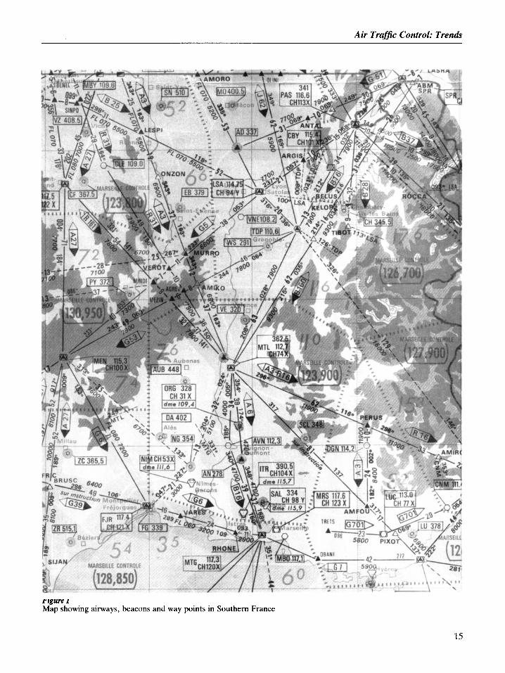
ATC assigns and controls the routes (and altitude or FL) in such a way that collisions are avoided and routes are as close to the routes requested in the flight plan as possible. The airspace is divided into regions (e.g., there are five regions over France); each region is divided into sectors (there are between eight and 12 sectors in a region), and each sector is monitored by one or two controllers. 1.1 Routes It could be surprising that traffic is voluntarily concen- trated on routes. This is the best way to monitor the motion of many planes in a three-dimensional space. Routes belong to controlled airspace; they are defined by the two points at the extremities of each leg (a leg is a straight line). These points, called way points (see Fig. l ) , could be (a) a radio beacon such as hf Omnirange for automatic

direction finder (ADF) or vhf Omnirange (VOR); (b) the intersection of two radials of VORs; (c) the bearing and the distance to a VOR (polar local

coordinates); or (d) the longitude/latitude.

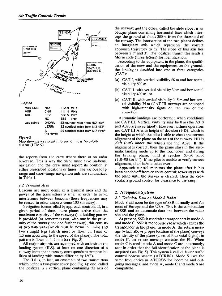
Routes are often designated by a number or a name; sometimes way points have a name coded with five letters; they are called reporting points when the crew must report passing over the way point (see Fig. 2). Additional information, such as minimum altitude or FL on the route, distance between the two way points and so on, are often indicated on maps.

ATC could have a precise position when the plane is flying in a space covered by radar but it can only rely on

14


Figure 1 Map showing airways, beacons and way points in Southern France

15

Air Trafjc Control: Trends

CNM 111.4 1-b

Legend VOR DME NlZ 112.4 MHz VOR CNM 111.4 MHz ADF LEZ 398.5 kHz

NC 338 kHz way paints : ONORA 22nautical miles from NIZ 1 9 2 O

LERlN 22 nautical miles frwn NIZ 1 8 3 O A 24 nautical miles from NIZ 225O (no mme)

Figure 2 Map showing way point information near Nice-CBte d'Azur (LFMN)

the reports from the crew where there is no radar coverage. This is why the plane must have on-board navigation and the crew must report its position at either prescribed locations or times. The various long- range and short-range navigation aids are summarized in Table 1.

1.2 Terminal Area Beacons are more dense in a terminal area and the power of the transmitters is small in order to avoid interference between beacons (these frequencies may be reused in other airports some 100 km away).

Navigation is controlled by approach controls. If, in a given period of time, more planes arrive than the maximum capacity of the runway(s), a holding pattern is provided (or sometimes two, with one in the proxi- mity of the runway and one further away); this consists of two half-turns (which must be flown in 1 min) and two straight legs (which must be flown in lmin or 1.5 min according to the speed of the plane). The total pattern is flown in 4-5 min (see Fig. 3).

All major airports are equipped with an instrument landing system (ILS), at least on one direction of a runway (note that a runway corresponds to two possibilities of landing with routes differing by 180").

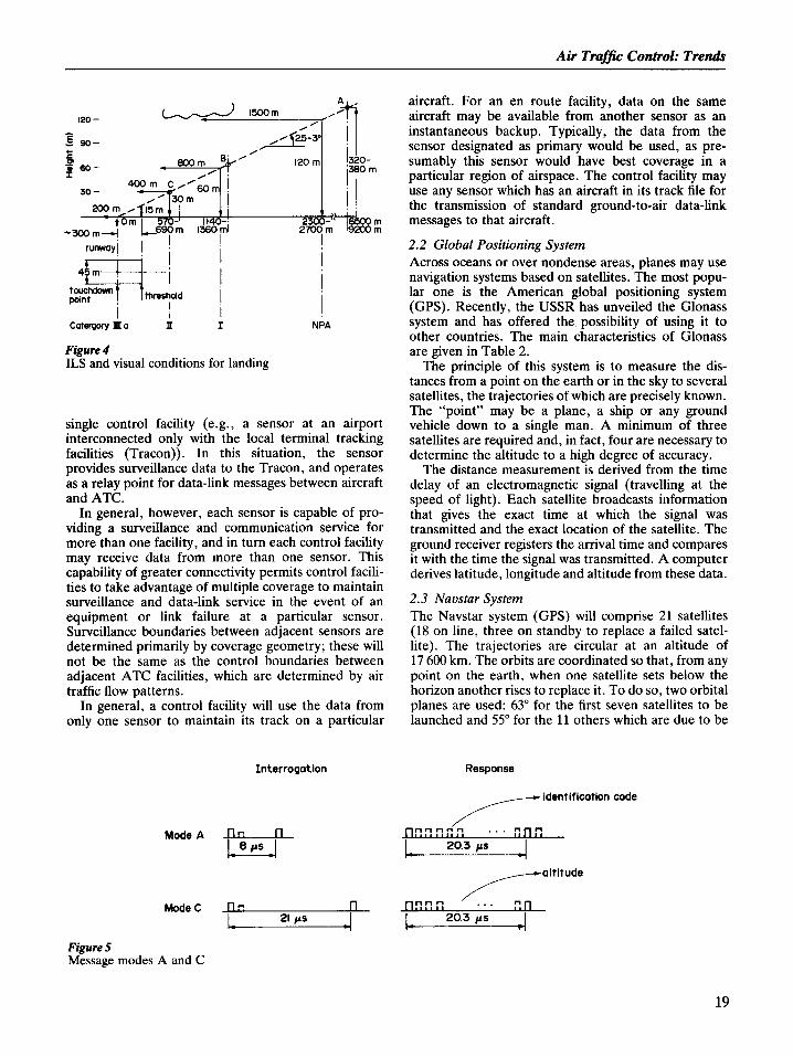
The ILS is, in fact, an ensemble of two transmitters which define a two-plane space (see Fig. 4): one, called the loca!izer, is a vertical plane containing the axis of

the runway; and the other, called the glide slope, is an oblique plane containing horizontal lines which inter- cept the ground at about 300 m from the threshold of the runway. The intersection of the two planes defines an imaginary axis which represents the correct approach trajectory to fly. The slope of this axis lies between 2.5" and 3". The localizer transmitter sends a Morse code (three letters) for identification.

According to the equipment in the plane, the qualifi- cation of the crew and the equipment on the ground, the landing is classified into one of three categories (CAT):

CAT I, with vertical visibility 60 m and horizontal visibility 800 m; CAT 11, with vertical visibility 30 m and horizontal visibility 400 m; or CAT 111, with vertical visibility 0-5 m and horizontal visibility 75 m (CAT I11 runways are equipped with high-intensity lights on the axis of the runway).

Automatic landings are performed when conditions are CAT 111. Vertical visibility may be 0 m (the A310 and A320 are so certified). However, airlines operators use CAT I11 A with height of decision (HD), which is the height at which the pilot is able to check the correct alignment of the plane on the axis of the runway. HD is 20ft (6m) under the wheels for the A320. If the alignment is correct, then the plane stays in the automatic landing mode up to the touchdown and during the braking phase, until it reaches 60-50 knot (110-90 km h-'). If the pilot is unable to verify correct alignment, then he/she takes over.

Approach control monitors the plane after it has been handed off from en route control; tower stays with the plane until the runway is cleared. Then the crew contacts ground control for clearance to the ramp.

2. Navigation Systems 2.1 Technical Data on Mode S Radar Mode S will soon be the type of SSR normally used for most of Europe and the USA. This is the combination of SSR and an automatic data link between the radar site and the plane.

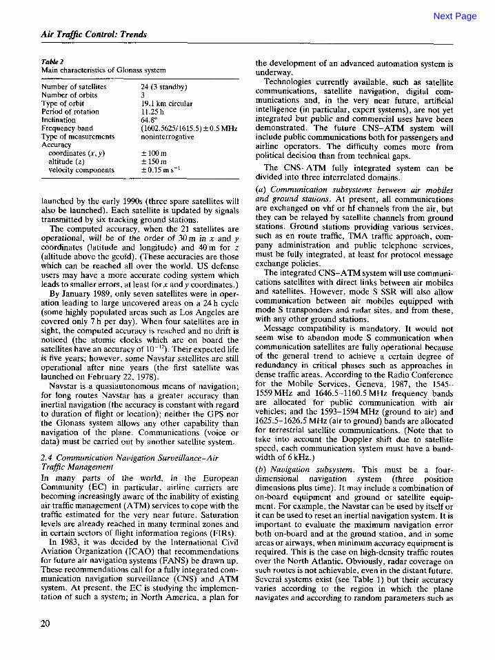
At present, SSR is used with transponders in mode A and mode C. SSR is monopulse radar which excites the transponder in the plane. In mode A , the return message (which allows proper location of the plane) conveys the identity of the plane (a set of four octal digits); in mode C, the return message contains the FL. When mode C is used, mode A and mode C are, alternately, sent in order that the full identification of the plane is acquired (see Fig. 5). This system is called the air traffic control beacon system (ATCRBS). Mode S uses the same frequencies as ATCRBS for incoming and out- going messages, and mode A, mode C and mode S are compatible.

16


The fundamental difference between mode S and ATCRBS is the manner of addressing aircraft or select- ing which aircraft will respond to an interrogation. In ACTRBS, the selection is spatial (i.e., aircraft within the mainbeam of the interrogator respond). As the beam sweeps around, all azimuths are interrogated, and all aircraft within line-of-sight of the antenna respond. In mode S, each aircraft is assigned a unique address code. This is a 24-bit address (which allows about 20 million different addresses to be assigned: a permanent address can thus be allocated to a plane when it is delivered).

Selection of which aircraft is to respond to an interrogation is accomplished by including the address code of the aircraft in the interrogation. Each such interrogation is thus directed to a particular aircraft.

Table I Navigation system comparisons

Narrow-beam antennas will continue to be used, but primarily for minimizing interference between sites and as an aid in the determination of aircraft azimuth.

An interrogator calls only those targets for which it has surveillance responsibility (this prevents saturation) and appropriate timing of interrogations avoids over- laps in answers (e.g., calls ordered according to the distance of the plane to the radar site).

There is provision in the messages for conveying additional data; this means that an automatic data link between ATC and plane potentially exists: 56 of the 112 bits of the interrogation or reply message are reserved for that purpose. Extended-length messages are also provided in up to 16 80-bit message segments.

The mode S-ATC interface is particularly simple in the case of an isolated mode S sensor interacting with a

Navigation Method used:

coordinates provided Coverage provided Status of the system

Navstar global positioning system

Transit

Loran type C or D

Omega

Automatic direction finder

VOR/DME Tacan

ILWmicrowave landing system (MLS)

Inertial navigation

Spherical ranging: Global three-dimensional position three-dimensional velocitv

(24 h d- ’)

Precise time

Doppler shift: longitude latitude

Hyperbolic ranging:

longitude latitude

Hyperbolic ranging:

longitude latitude

Goniometry on omnidirectional beacon

Six satellites in 12 h orbits, available worldwide 1-4 h d-‘

Global except at the poles (periodic fixes only, typically f-2 h apart)

Five satellites in polar “birdcage” orbits; more than 10 OOO sets in use, with 80% civilian users

Regional, coverage about Eight loran C chains with 34 transmitters cover about 10% of the earth

10% of earth

Essentially global: 88% Eight transmitting stations in coverage by day, 98% by night

operation worldwide

100 nautical miles around the Worldwide beacon, not accurate in case of storm (lightning)

Lighthouse signal and Line of sight along present air More than 1OOO transmitters spherical ranging: routes in operation; at least

he ad i n g slant range

250 OOO users

Beam Steering: heading elevation range

Line of sight: 17-35 nautical miles, available only at properly equipped airports

Hundreds of systems operating worldwide; more than 120 OOO domestic users

Integrating Global with periodic updates Thousands of self-contained accelerometers:

position

units in use on civilian and three-dimensional military planes and ships

three-dimensional velocity

17

Figure 3 Approach landing sy! defined by

APPROCHE TTTTTTProtbge6 pour Cat. A B C D

NICE-C8te d'Azur (LFMN) A l t -Ad : 13, Seuil : I 3 ( I hPa)

avant d'odl6rer en d plus de 2OOO (1987)

LERIN cu DRAMO/L - LLZ -1M Rwy 0 5 L 02-NICE-Cote dhzur (LFMN) 880211 - v

to Nice-CBte d'Azur (as Fig. 2), runway 05R (actual magnetic bearing 046", R means right) instrun stem (ILS) with two possibilities: from the LERIN or DRAM0 stackings (note that these two stack way points which do not correspond to a radioelectric beacon)

lent Lings are

18

Air Trafjc Control: Trends

120 - 1500m

Caterpory ma I[ I NPA

Figure 4 ILS and visual conditions for landing

single control facility (e.g., a sensor at an airport interconnected only with the local terminal tracking facilities (Tracon)). In this situation, the sensor provides surveillance data to the Tracon, and operates as a relay point for data-link messages between aircraft and ATC.

In general, however, each sensor is capable of providing a surveillance and communication service for more than one facility, and in turn each control facility may receive data from more than one sensor. This capability of greater connectivity permits control facilities to take advantage of multiple coverage to maintain surveillance and data-link service in the event of an equipment or link failure at a particular sensor. Surveillance boundaries between adjacent sensors are determined primarily by coverage geometry; these will not be the same as the control boundaries between adjacent ATC facilities, which are determined by air traffic flow patterns.

In general, a control facility will use the data from only one sensor to maintain its track on a particular

Mode A

Mode C

aircraft. For an en route facility, data on the same aircraft may be available from another sensor as an instantaneous backup. Typically, the data from the sensor designated as primary would be used, as pre- sumably this sensor would have best coverage in a particular region of airspace. The control facility may use any sensor which has an aircraft in its track file for the transmission of standard ground-to-air data-link messages to that aircraft.

2.2 Global Positioning System Across oceans or over nondense areas, planes may use navigation systems based on satellites. The most popu- lar one is the American global positioning system (GPS). Recently, the USSR has unveiled the Glonass system and has offered the possibility of using it to other countries. The main characteristics of Glonass are given in Table 2.

The principle of this system is to measure the dis- tances from a point on the earth or in the sky to several satellites, the trajectories of which are precisely known. The “point” may be a plane, a ship or any ground vehicle down to a single man. A minimum of three satellites are required and, in fact, four are necessary to determine the altitude to a high degree of accuracy.

The distance measurement is derived from the time delay of an electromagnetic signal (travelling at the speed of light). Each satellite broadcasts information that gives the exact time at which the signal was transmitted and the exact location of the satellite. The ground receiver registers the arrival time and compares it with the time the signal was transmitted. A computer derives latitude, longitude and altitude from these data.

2.3 Naustar System The Navstar system (GPS) will comprise 21 satellites (18 on line, three on standby to replace a failed satellite). The trajectories are circular at an altitude of 17 600 km. The orbits are coordinated so that, from any point on the earth, when one satellite sets below the horizon another rises to replace it. To do so, two orbital planes are used: 63” for the first seven satellites to be launched and 55” for the 11 others which are due to be

Interrogation Response

y identification code

/ n m n n m . . . n n n

I 20.3 ss I

/-----a’titude n ... nn /

n nnn n

L 4 L 21 ps 20.3 ps 4 Figure 5 Message modes A and C

19

Air Trafjic Control: Trends

Table 2 Main characteristics of Glonass system

Number of satellites Number of orbits Type of orbit Period of rotation Inclination Frequency band Type of measurements Accuracy

coordinates ( x , y ) altitude (2) velocity components

24 ( 3 standby) 3 19.1 km circular 11.25 h 64.e (1602.5625/1615.5) k 0.5 MHz noninterrogative

k 100 m k 150 m f0 .15rns- l

launched by the early 1990s (three spare satellites will also be launched). Each satellite is updated by signals transmitted by six tracking ground stations.

The computed accuracy, when the 21 satellites are operational, will be of the order of 30m in x and y coordinates (!atitude and longitude) and 40m for z (altitude above the geoid). (These accuracies are those which can be reached all over the world. US defense users may have a more accurate coding system which leads to smaller errors, at least for x and y coordinates.)

By January 1989, only seven satellites were in operation leading to large uncovered areas on a 24 h cycle (some highly populated areas such as Los Angeles are covered only 7 h per day). When four satellites are in sight, the computed accuracy is reached and no drift is noticed (the atomic clocks which are on board the satellites have an accuracy of lo-'*). Their expected life is five years; however, some Navstar satellites are still operational after nine years (the first satellite was launched on February 22, 1978).

Navstar is a quasiautonomous means of navigation; for long routes Navstar has a greater accuracy than inertial navigation (the accuracy is constant with regard to duration of flight or location); neither the GPS nor the Glonass system allows any other capability than navigation of the plane. Communications (voice or data) must be carried out by another satellite system.

2.4 Communication Navigation Surveillance-Air TrafJic Management In many parts of the world, in the European Community (EC) in particular, airline carriers are becoming increasingly aware of the inability of existing air traffic management (ATM) services to cope with the traffic estimated for the very near future. Saturation levels are already reached in many terminal zones and in certain sectors of flight information regions (FIRS).

In 1983, it was decided by the International Civil Aviation Organization (ICAO) that recommendations for future air navigation systems (FANS) be drawn up. These recommendations call for a fully integrated communication navigation surveillance (CNS) and ATM system. At present, the EC is studying the implementation of such a system; in North America, a plan for

the development of an advanced automation system is underway.

Technologies currently available, such as satellite communications, satellite navigation, digital communications and, in the very near future, artificial intelligence (in particular, expert systems), are not yet integrated but public and commercial uses have been demonstrated. The future CNS-ATM system will include public communications both for passengers and airline operators. The difficulty comes more from political decision than from technical gaps.

The CNS-ATM fully integrated system can be divided into three interrelated domains. ( a ) Communication subsystems between air mobiles and ground stations. At present, all communications are exchanged on vhf or hf channels from the air, but they can be relayed by satellite channels from ground stations. Ground stations providing various services, such as en route traffic, TMA traffic approach, company administration and public telephone services, must be fully integrated, at least for protocol message exchange policies.

The integrated CNS-ATM system will use communications satellites with direct links between air mobiles and satellites. However, mode S SSR will also allow communication between air mobiles equipped with mode S transponders and radar sites, and from these, with any other ground stations.

Message compatibility is mandatory. It would not seem wise to abandon mode S communication when communication satellites are fully operational because of the general trend to achieve a certain degree of redundancy in critical phases such as approaches in dense traffic areas. According to the Radio Conference for the Mobile Services, Geneva, 1987, the 1545- 1559 MHz and 1646.5-1160.5 MHz frequency bands are allocated for public communication with air vehicles; and the 1593-1594MHz (ground to air) and 1625.5-1626.5 MHz (air to ground) bands are allocated for terrestrial satellite communications. (Note that to take into account the Doppler shift due to satellite speed, each communication system must have a band- width of 6 kHz.) (b) Navigation subsystem. This must be a four- dimensional navigation system (three position dimensions plus time). It may include a combination of on-board equipment and ground or satellite equipment. For example, the Navstar can be used by itself or it can be used to reset an inertial navigation system. It is important to evaluate the maximum navigation error both on-board and at the ground station, and in some areas or airways, when minimum accuracy equipment is required. This is the case on high-density traffic routes over the North Atlantic. Obviously, radar coverage on such routes is not achievable, even in the distant future. Several systems exist (see Table 1) but their accuracy varies according to the region in which the plane navigates and according to random parameters such as

20

Next Page

Date post:	28-Nov-2015
Category:	Documents
Upload:	grenouille2
View:	29 times
Download:	1 times

Air Traffic Control

Documents