Airborne UXO Surveys Using the MTADS - SERDP … · Airborne UXO Surveys Using the MTADS ... 1.1.1...

Approved for public release; distribution is unlimited.

Naval Research LaboratoryWashington, DC 20375-5320

April 5, 2005

NRL/MR/6110--05-8874

Airborne UXO Surveys Usingthe MTADS

H. H. NELSON

Chemical Dynamics and Diagnostics BranchChemistry Division

J. R. MCDONALD

DAVID WRIGHT

AETC, Inc.Cary, NC

i

REPORT DOCUMENTATION PAGE Form Approved

OMB No. 0704-0188

3. DATES COVERED (From - To)

Standard Form 298 (Rev. 8-98)Prescribed by ANSI Std. Z39.18

Public reporting burden for this collection of information is estimated to average 1 hour per response, including the time for reviewing instructions, searching existing data sources, gathering andmaintaining the data needed, and completing and reviewing this collection of information. Send comments regarding this burden estimate or any other aspect of this collection of information, includingsuggestions for reducing this burden to Department of Defense, Washington Headquarters Services, Directorate for Information Operations and Reports (0704-0188), 1215 Jefferson Davis Highway,Suite 1204, Arlington, VA 22202-4302. Respondents should be aware that notwithstanding any other provision of law, no person shall be subject to any penalty for failing to comply with a collection ofinformation if it does not display a currently valid OMB control number. PLEASE DO NOT RETURN YOUR FORM TO THE ABOVE ADDRESS.

5a. CONTRACT NUMBER

5b. GRANT NUMBER

5c. PROGRAM ELEMENT NUMBER

5d. PROJECT NUMBER

5e. TASK NUMBER

5f. WORK UNIT NUMBER

2. REPORT TYPE1. REPORT DATE (DD-MM-YYYY)

4. TITLE AND SUBTITLE

6. AUTHOR(S)

8. PERFORMING ORGANIZATION REPORT

NUMBER

7. PERFORMING ORGANIZATION NAME(S) AND ADDRESS(ES)

10. SPONSOR / MONITOR’S ACRONYM(S)9. SPONSORING / MONITORING AGENCY NAME(S) AND ADDRESS(ES)

11. SPONSOR / MONITOR’S REPORT

NUMBER(S)

12. DISTRIBUTION / AVAILABILITY STATEMENT

13. SUPPLEMENTARY NOTES

14. ABSTRACT

15. SUBJECT TERMS

16. SECURITY CLASSIFICATION OF:

a. REPORT

19a. NAME OF RESPONSIBLE PERSON

19b. TELEPHONE NUMBER (include area

code)

b. ABSTRACT c. THIS PAGE

18. NUMBER

OF PAGES

17. LIMITATION

OF ABSTRACT

05-04-2005

Airborne UXO Surveys Using the MTADS

Naval Research Laboratory, Code 61104555 Overlook Avenue, SWWashington, DC 20375-5320

An airborne version of the MTADS vehicular towed array has been developed and demonstrated with the support of ESTCP Project 200031.The system is ideally suited to localizing burial caches of ordnance and establishing areas that are uncontaminated but also retains the capabilityof detecting, locating, and identifying individual ordnance items the size of 2.75-in. rocket warheads and larger. The system deploys a linear arrayof 7 Cs-vapor magnetometers spaced at 1.5-m intervals in a forward-mounted boom on a Bell Long Ranger helicopter. Two GPS units mounted onthe forward boom provide positioning and roll and yaw measurements. An inertial measurement unit and a 3-axis fluxgate gradiometer redun-dantly provide additional attitude measurements. Laser, radar, and acoustic altimeters provide altitude information. A pilot guidance displayprovides survey progress and platform information in real time. All sensor data are recorded in a data acquisition computer mounted in one of thehelicopter rear seats. This report documents the performance of the Airborne MTADS at three ranges containing both live ordnance and inert,seeded ordnance.

Unclassified Unclassified UnclassifiedUL 140

Herbert H. Nelson

(202) 767-3686

Multi-sensor Towed Array Detection System (MTADS); Airborne magnetometry; Unexploded ordnance (UXO); UXO detection

Memorandum report

Environmental Security Technology Certification ProgramAttn: Dr. Anne Andrews901 North Stuart Street, Suite 303Arlington, VA 22203

NRL/MR/6110--05-8874

Approved for public release; distribution is unlimited.

*AETC, Inc., Cary, NC 27513Accompanying CD (on inside back cover) contains this Memorandum Report.

March 2000-January 2004

H. H. Nelson, J. R. McDonald,* and David Wright*

ESTCP

ESTCP Project 200031

61-5802

iii

CONTENTS Figures............................................................................................................................................ ix

Tables........................................................................................................................................... xiii

Acronyms...................................................................................................................................... xv

Executive Summary ......................................................................................................................E1

1. Introduction............................................................................................................................. 1

1.1 Background..................................................................................................................... 1

1.1.1 The UXO Problem .................................................................................................. 1

1.1.2 Automated Geo-referenced Surveys ....................................................................... 1

1.1.3 The Airborne System .............................................................................................. 3

1.2 Objectives of the ESTCP Demonstrations...................................................................... 4

1.2.1 Prior MTADS Demonstrations ............................................................................... 4

1.2.2 Overall Development Objectives............................................................................ 4

1.2.3 Demonstration Support and Coordination .............................................................. 5

1.3 Regulatory Issues ............................................................................................................ 5

2. Technology Description.......................................................................................................... 7

2.1 Technology Development and Application .................................................................... 7

2.1.1 System Specifications and Requirements ............................................................... 7

2.1.2 Field Hardware........................................................................................................ 7

2.1.3 Data Preprocessing................................................................................................ 10

2.1.4 Data Analysis ........................................................................................................ 15

2.2 Previous Testing of the Technology ............................................................................. 17

2.3 Factors Affecting Cost and Performance...................................................................... 17

2.4 Advantages and Limitations of the Technology ........................................................... 18

iv

3. BBR Demonstration.............................................................................................................. 21

3.1 Performance Objectives ................................................................................................ 21

3.1.1 BBR Demonstration Objectives............................................................................ 21

3.2 Selection of the Demonstration Site ............................................................................. 22

3.3 Test Site History and Characteristics............................................................................ 22

3.3.1 Site and Facility History ....................................................................................... 22

3.3.2 Site and Facility Maps and Photographs............................................................... 23

3.4 Previous UXO Clearances ............................................................................................ 23

3.4.1 The 1975 Clearance .............................................................................................. 23

3.4.2 The 1997 Clearance .............................................................................................. 26

3.5 Testing and Evaluation Plan ......................................................................................... 27

3.5.1 Demonstration Setup and Operation..................................................................... 27

3.6 Results........................................................................................................................... 31

3.6.1 Overview............................................................................................................... 31

3.6.2 The Seed Target Surveys ....................................................................................... 33

3.6.3 The South, West, and North Surveys.................................................................... 38

3.6.4 Comparative Performance of the Two Systems.................................................... 39

3.6.5 The Airborne Production Survey .......................................................................... 42

3.6.6 Performance Assessment ...................................................................................... 46

3.6.7 Technology Performance Comparison ................................................................. 48

3.7 Cost Assessment ........................................................................................................... 48

3.7.1 Cost Performance.................................................................................................. 48

3.7.2 Cost Comparison................................................................................................... 49

3.8 Technology Implementation ......................................................................................... 51

v

3.8.1 DoD Need ............................................................................................................. 51

3.8.2 Transition .............................................................................................................. 51

3.9 Lessons Learned............................................................................................................ 52

4. APG Demonstration.............................................................................................................. 53


4.2 Selecting Test Sites ....................................................................................................... 53

4.3 Test Site History/Characteristics................................................................................... 54

4.4 Present Operations ........................................................................................................ 54

4.5 Pre-demonstration Testing and Analysis ...................................................................... 54

4.5.1 Site Preparation..................................................................................................... 54

4.5.2 Changes in the MTADS........................................................................................ 54


4.6.1 Pre-demonstration Site Preparation ...................................................................... 55

4.6.2 The APG Seed Target Plan ................................................................................... 55

4.6.3 The APG Designated Survey Areas...................................................................... 55

4.6.4 Period of Operation............................................................................................... 62

4.6.5 Area Characterized or Remediated ....................................................................... 63

4.6.6 Operating Parameters for the Technology ............................................................ 63

4.6.7 APG Demonstration Organizations and Personnel............................................... 64

4.6.8 Survey Experimental Design ................................................................................ 65

4.7 Survey Results .............................................................................................................. 67

4.7.1 The Airfield Survey .............................................................................................. 67

4.7.2 The Active Recovery Field Survey....................................................................... 70

4.7.3 The Dewatering Ponds.......................................................................................... 72

vi

4.7.4 The Mine, Grenade, and Direct Fire Weapons Range .......................................... 76

4.7.5 The Chesapeake Bay Impact Range ..................................................................... 77

4.8 Performance .................................................................................................................. 78

4.8.1 Performance Criteria............................................................................................. 78

4.8.2 Performance at the Airfield................................................................................... 79

4.8.3 The Active Recovery Field ................................................................................... 80

4.8.4 The Dewatering Ponds.......................................................................................... 86

4.9 Cost Assessment ........................................................................................................... 87

4.9.1 Cost Reporting ...................................................................................................... 87

4.9.2 Cost Tracking........................................................................................................ 88

4.9.3 Cost Analysis ........................................................................................................ 88

4.9.4 Cost Comparison................................................................................................... 90

4.9.5 Implementation (Technology Transfer ................................................................. 90

5. Isleta Demonstration ............................................................................................................. 93


5.2 Selecting the Test Site................................................................................................... 95

5.3 Test Site Characteristics and History............................................................................ 95

5.3.1 Site Characteristics................................................................................................ 95

5.3.2 Site History ........................................................................................................... 96

5.3.3 Climate and Weather............................................................................................. 96

5.3.4 Site Maps and Photographs................................................................................... 96

5.3.5 Present Operations ................................................................................................ 96


5.4.1 Pre-demonstration Activities ................................................................................ 97

vii

5.4.2 Period of Operation............................................................................................... 97

5.4.3 Area Characterized................................................................................................ 99

5.4.4 Area Remediated................................................................................................. 102

5.4.5 Operating Parameters for the Technology .......................................................... 104

5.4.6 Survey Experimental Design .............................................................................. 104

5.5 Survey Results ............................................................................................................ 104

5.6 System Performance ................................................................................................... 105

5.6.1 Performance Against Emplaced Targets............................................................. 106

5.6.2 Vehicular Area Remediated Targets................................................................... 107

5.6.3 Targets Remediated in the Primary Area............................................................ 109

5.6.4 Reinvestigation of “No Finds” in the Primary Area. .......................................... 109

5.7 Cost Assessment ......................................................................................................... 110

6. Cost Assessment ................................................................................................................. 115

7. References........................................................................................................................... 117

8. Points of Contact................................................................................................................. 121

viii

ix

FIGURES

1. Airborne MTADS survey hardware is shown being installed on a Bell Long Ranger at the Helicopter Transport Services hangar.................................................................................8

2. Airborne MTADS survey on the Active Recovery Field. Note the 2-meter high vegetation that stretches from this point to the shoreline .........................................................8

3. The DAQ console is shown mounted in the rear starboard seat position. Note the Trimble Model MS-750 units mounted on the side of the rack................................................8

4. The navigation guidance display is mounted on the starboard side of the cockpit for the pilot’s use during surveys .......................................................................................................10

5. Close-up of the pilot navigation display screen showing the pilot lining up on line 11 (red) of the survey grid ..........................................................................................................10

6. Working screen of the MTADS DAS showing the survey project view on the left and an expanded analysis window on the right..................................................................................11

7. A working screen of Oasis montaj™ showing airborne data from the Isleta demonstrations........................................................................................................................11

8. An unfiltered power spectrum (left panel) is shown for sensor 6. One hour of data is included, which was taken during the survey of the Active Recovery Field. The right panel shows the same data after notch filtering to remove blade noise..................................12

9. Important components of the sensor boom involved in deriving the Digital Elevation Model......................................................................................................................................14

10. Schematic of the sensor boom showing the GPS, laser, and acoustic altimeters used to derive the DEM.......................................................................................................................15

11. Site view and data analysis screens from the MTADS data analysis program. A part of the Mine, Grenade, and Direct-Fire Weapons Range survey is shown on the left. An individual target is boxed for analysis on the right.................................................................16

12. The target fit window from the MTADS DAS. Data from the target boxed in Figure 11 are shown on the left. The dipole model fit is shown on the right. Fit parameters are shown in the left and center columns. Advanced processing options are indicated in the right column, where the analyst’s comments are also recorded. ............................................17

13. The BBR Impact Area lies within the red boundary. The 1999 survey is shown in green. The 10-acre seed target area, bounded by a thinner red border, lies within this area.............24

x

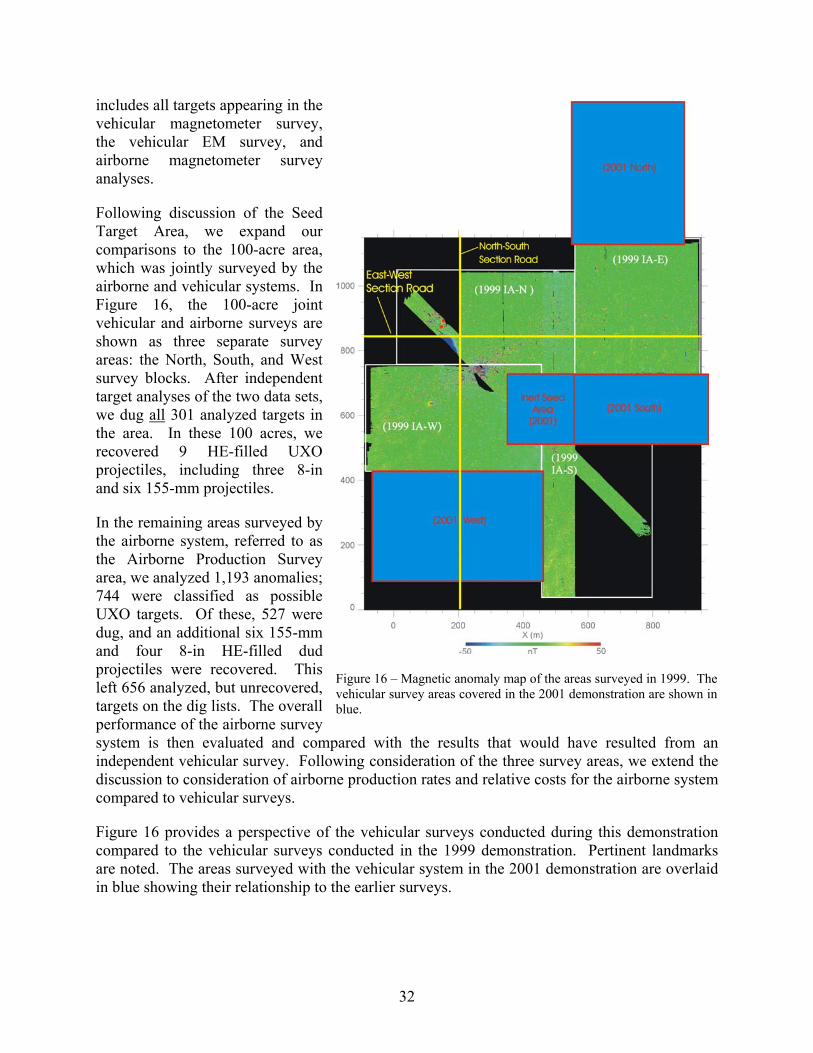
14. Plot of the area surveyed using the vehicular MTADS in 1999 is shown in green. The seeded target area for the 2001 demonstration was mostly surveyed and dug during the 1999 survey.............................................................................................................................25

15. Logistics setup supporting the demonstration at the Impact Area..........................................29

16. Magnetic anomaly map of the areas surveyed in 1999. The vehicular survey areas covered in the 2001 demonstration are shown in blue. ..........................................................32

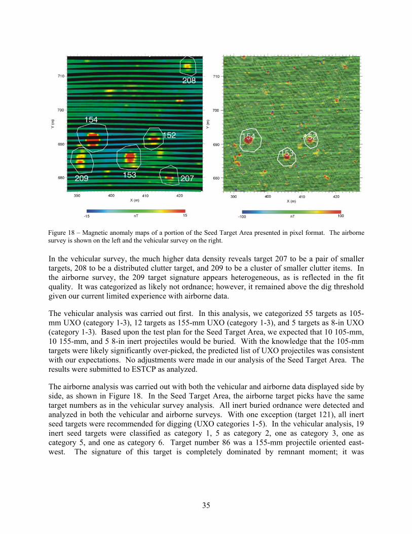
17. Magnetic anomaly images of the Seed Target Area from the airborne survey on the left and the vehicular survey on the right. The Seed Target Area is 200 × 200 meters; the southwest corner coordinates are X =360 m, Y = 530 m .......................................................34

18. Magnetic anomaly maps of a portion of the Seed Target Area presented in pixel format. The airborne survey is shown on the left and the vehicular survey on the right ....................35

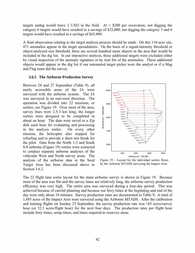
19. Layout for the individual sorties flown by the Airborne MTADS surveying the Impact Area.........................................................................................................................................42

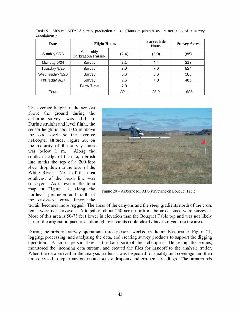
20. Airborne MTADS surveying on Bouquet Table ....................................................................43

21. The MTADS data analysis trailer ...........................................................................................44

22. Magnetic anomaly image for the Airborne MTADS survey of the Impact Area...................45

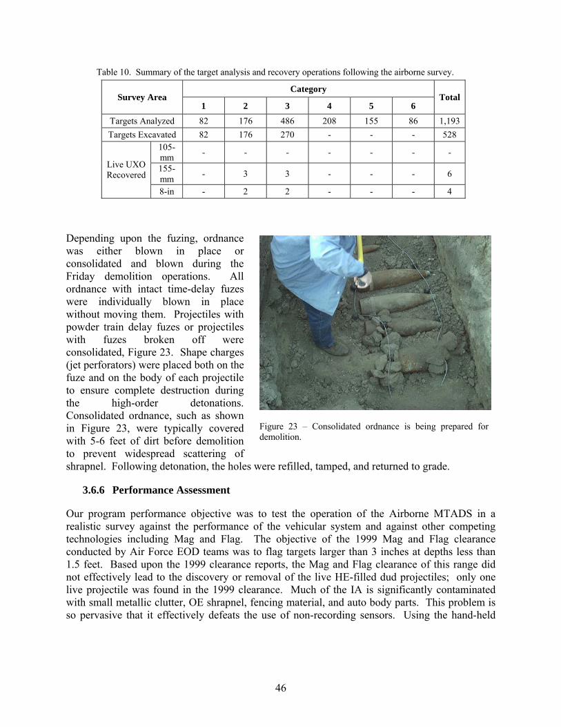
23. Consolidated ordnance is being prepared for demolition .......................................................46

24. ROC curves for the vehicular and airborne surveys on the 110-acre vehicular survey area..47

25. Digital orthophoto of a portion of the Airfield near the south end of Runway 35. The areas outlined by dark red rectangles are the designated survey areas. Calibration targets were installed east of the runway. The area south of the runway was the primary survey area. The panel on the right has the MTADS DEM superimposed on both survey areas .....54

26. Oblique aerial photo of the part of the Dewatering Ponds Area. The four small ponds in the foreground and the large pond to the immediate upper right were included in this survey......................................................................................................................................56

27. MTADS survey over the large pond.......................................................................................57

28. MTADS survey over one of the Finger Ponds ......................................................................58

29. Digital orthophoto of the Dewatering Ponds with the MTADS DEM superimposed over the 5 survey ponds. Note the four finger ponds in the lower left corner ...............................58

xi

30. Aerial photo, looking approximately west to east, shows the Active Recovery Field. The impact area includes the cleared area and offshore areas that may extend for an additional several hundred meters beyond the shoreline........................................................59

31. Clusters of ordnance exist on the surface at various points on the Active Recovery Field....60

32. Stockpiles of ordnance and scrap along the roads at the Active Recovery Field ...................60

33. Digital orthophoto of the Active Recovery Field is shown on the left. On the right, the DEM from the MTADS survey is shown ...............................................................................61

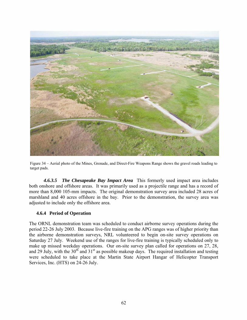
34. Aerial photo of the Mines, Grenade, and Direct-Fire Weapons Range shows the gravel roads leading to target pads ....................................................................................................62

35. A 4-second data clip for sensor 1 at the airfield seed target survey showing the effects of the filters used for reprocessing the data ................................................................................65

36. MTADS analysis windows are shown for a section of the Airfield seed target survey. On the left, the data are shown as originally submitted. On the right, data are shown following reprocessing using the low-pass filter as described in the text ..............................66

37. MTADS magnetic anomaly image from the airborne survey of the Calibration Target Area.........................................................................................................................................67

38. Pixel image plot (subsampled) of the Airborne MTADS survey of the Airfield. The white border defines the limits of the survey. See Figure 11 for the DOQ and DEM presentations ...........................................................................................................................68

39. ROC curves for the Airfield open-field area for a 1.5 m halo................................................69

40. Magnetic anomaly image (interpolated) of the Active Recovery Range. Note the cluster of surface ordnance at the top center, stockpiles of materials along the road, and the extended concentration of magnetic returns offshore.............................................................71

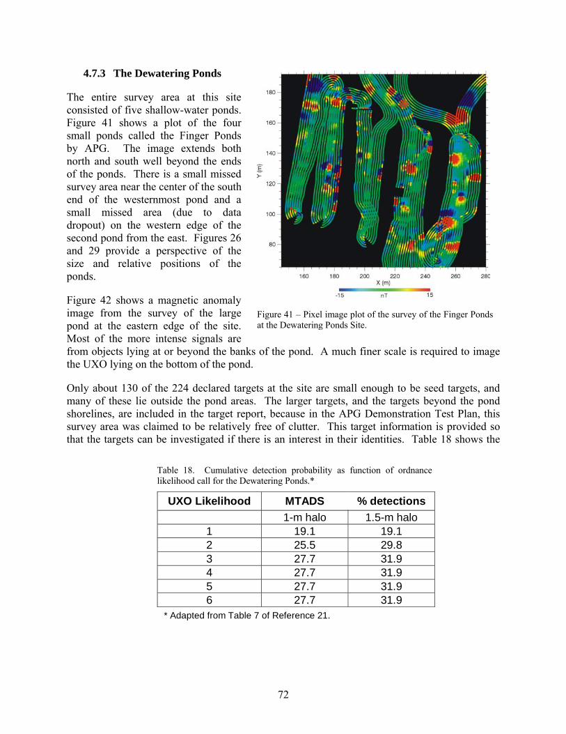
41. Pixel image plot of the survey of the Finger Ponds................................................................72

42. Magnetic anomaly (subsampled, pixel) image from the survey of the large Dewatering Pond ........................................................................................................................................74

43. MTADS survey image of the Mine, Grenade, and Direct-Fire Weapons Range ...................76

44. Magnetic anomaly image of a portion of the Mine, Grenade, and Direct-Fire Weapons Range showing the target pad near the north corner of the survey in Figure 33....................76

45. Magnetic anomaly image (interpolated) of the Chesapeake Bay Impact Range....................77

xii

46. Pixel image (subsampled) of an area near the south end of the offshore survey showing individual target signatures.....................................................................................................77

47. A portion of a USGS topo map showing the boundaries of the planned surveys. The locations of the two first-order points installed on this site for the surveys are shown as 1A and 1B...............................................................................................................................94

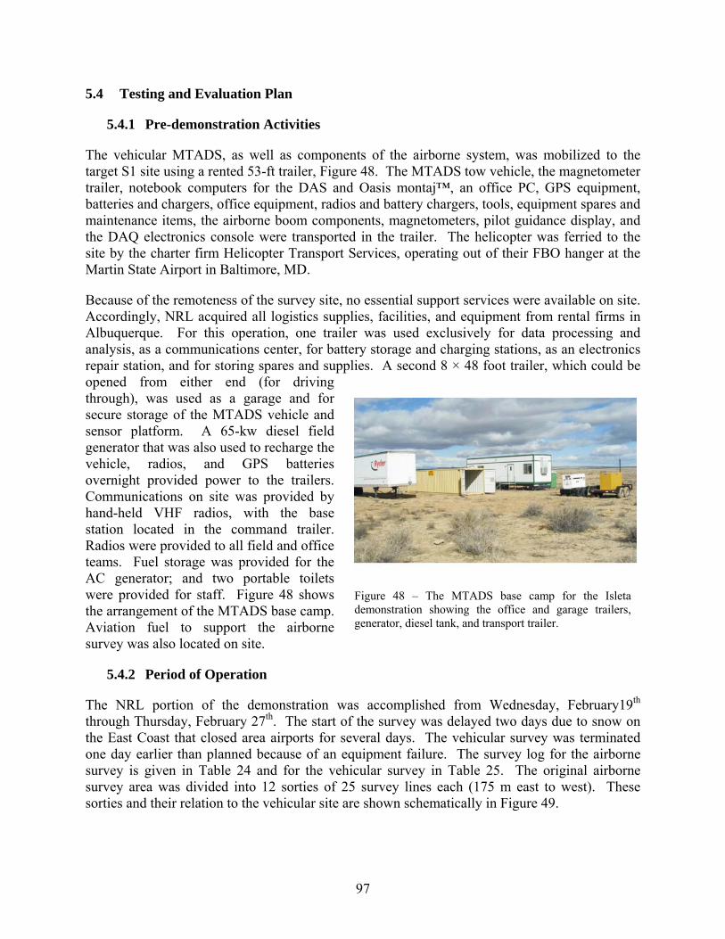
48. The MTADS base camp for the Isleta demonstration showing the office and garage trailers, generator, diesel tank, and transport trailer ...............................................................97

49. Planned layout of the Isleta airborne survey. The planned vehicular MTADS survey bounds are shown in black....................................................................................................100

50. Magnetic anomaly map from the vehicular survey superimposed on the USGS topo map of the area .............................................................................................................................101

51. Magnetic anomaly map of the Isleta airborne survey. The vehicular survey areas are outlined by the smaller yellow rectangles. The Primary Area is outlined by the large yellow rectangle....................................................................................................................103

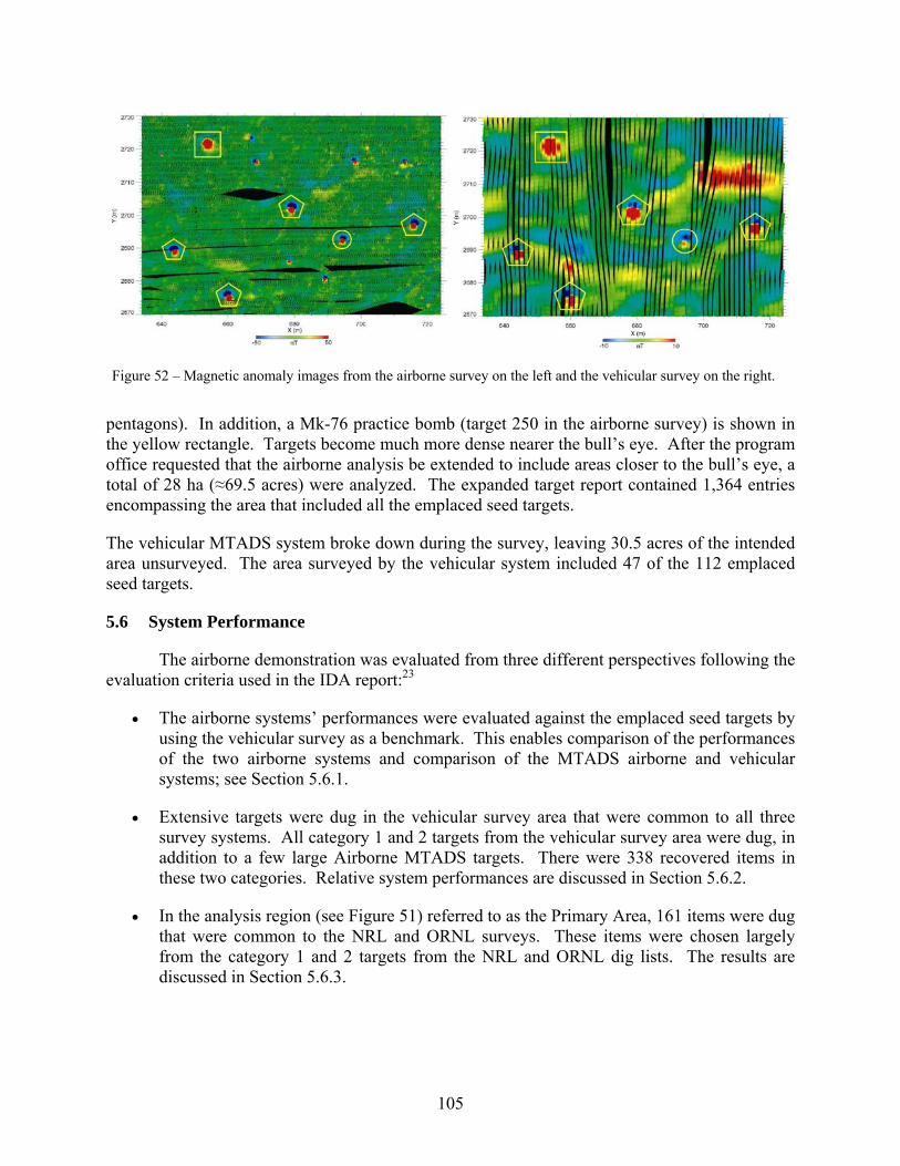
52. Magnetic anomaly images from the airborne survey on the left and the vehicular survey on the right............................................................................................................................105

53. ROC curves for emplaced ordnance detection .....................................................................106

54. Airborne MTADS location error scatter plot for the seed targets ........................................107

55. ROC curves for the targets remediated in the vehicular area ...............................................108

56. Scatter plots showing the location performance of the vehicular and Airborne MTADS for the remediated targets in the vehicular area....................................................................108

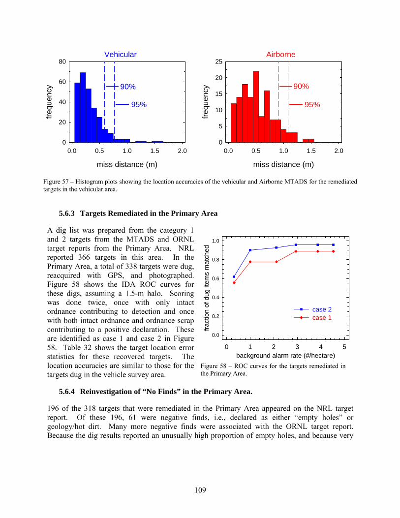
57. Histogram plots showing the location accuracies of the vehicular and Airborne MTADS for the remediated targets in the vehicular area....................................................................109

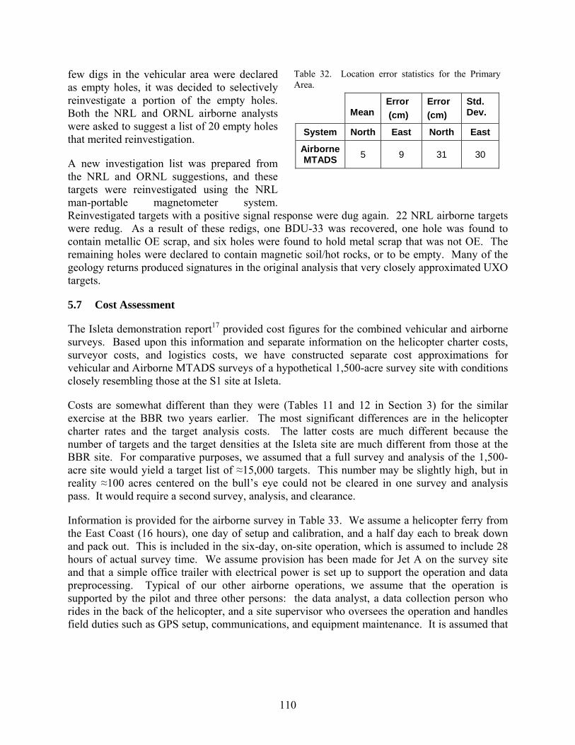
58. ROC curves for the targets remediated in the Primary Area ................................................109

xiii

TABLES

1. System Specifications and Requirements for the Airborne MTADS.......................................7

2. Impact Area survey coordinates provided by Ellsworth AFB................................................23

3. Recovered and documented ordnance items from the IA in the 1997 clearance....................26

4. Ground truth table for the inert seed ordnance emplaced at the Impact Area ........................28

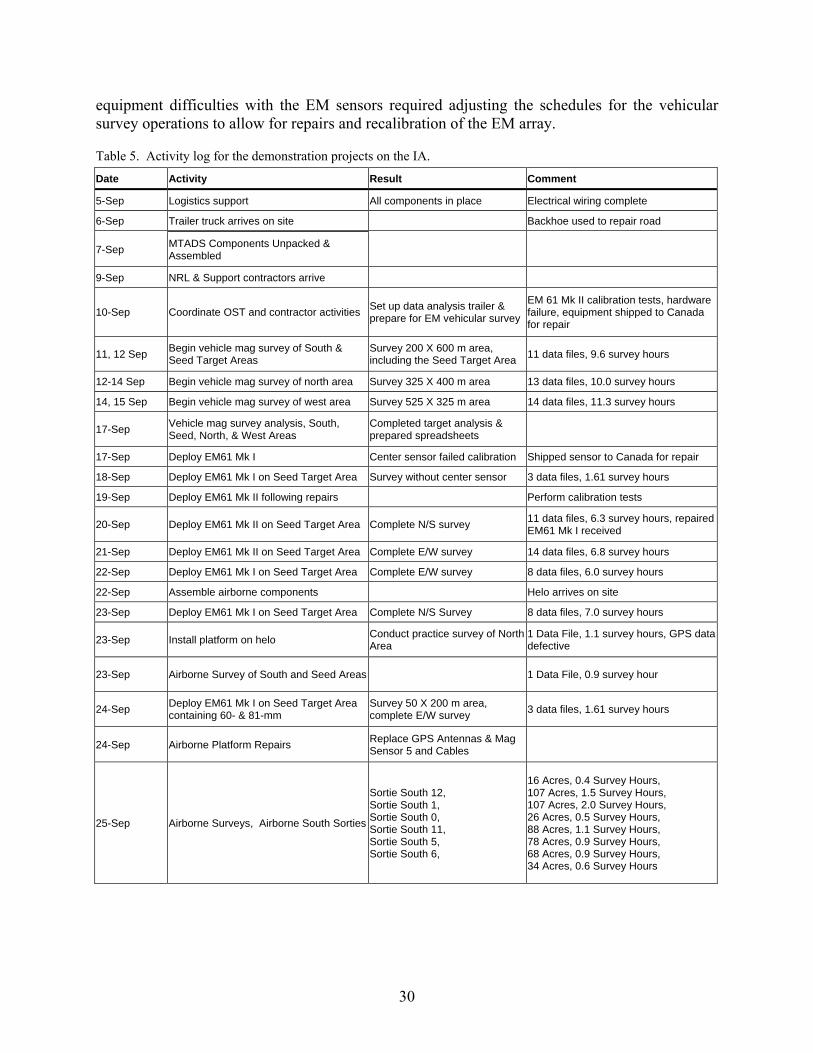
5. Activity log for the demonstration projects on the IA............................................................30

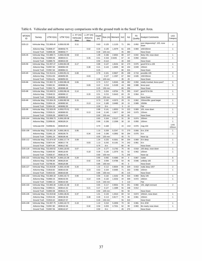
6. Vehicular and Airborne Survey Comparisons with the Ground Truth in the Seed Target Area.........................................................................................................................................37

7. Summary of UXO recovery information in the vehicular MTADS survey ...........................40

8. Summary of all the vehicular and airborne target analyses for the North, West, and South blocks and the Seed Target Area ............................................................................................41

9. Airborne MTADS Survey Production Rates. Hours in parentheses are not included in survey calculations..................................................................................................................43

10. Summary of the target analysis and recovery operations following the airborne survey.......46

11. Projected costs for a 1500-acre Airborne MTADS survey.....................................................49

12. Projected costs for a 1500-acre vehicular MTADS survey ....................................................50

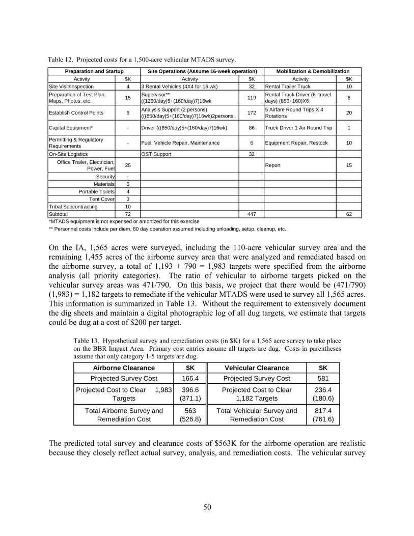
13. Hypothetical survey and remediation costs (in $K) for a 1,565 acre survey to take place on the BBR Impact Area. Primary cost entries assume all targets are dug. Costs in parentheses assume that only category 1-5 targets are dug ....................................................50

14. Airborne MTADS survey and flight production summary.....................................................63

15. Ordnance detection results for the Airfield open field area for three detection halos ............69

16. Ordnance detection results for Active Recovery Field for two detection halos .....................70

17. Cumulative detection probability as function of ordnance likelihood call for the Active Recovery Field........................................................................................................................70

18. Cumulative detection probability as function of ordnance likelihood call for the dewatering ponds ....................................................................................................................72

xiv

19. Ground Truth for the targets emplaced in the Dewatering Ponds ..........................................75

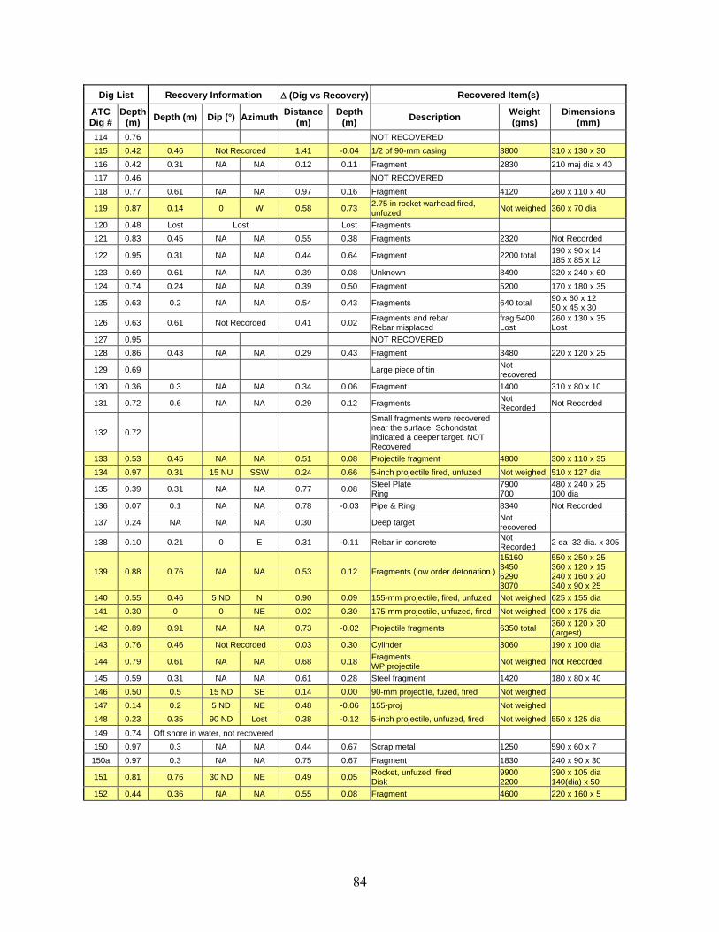
20. Active Recovery Field UXO Dig Results...............................................................................81

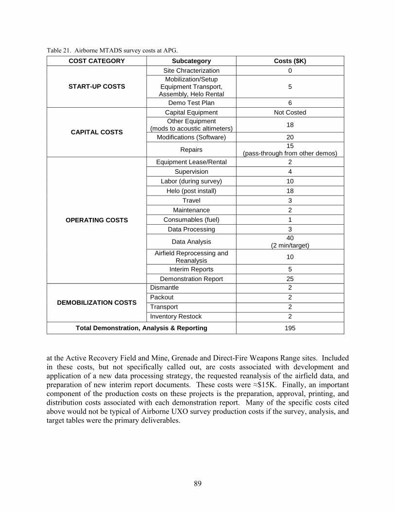
21. Airborne MTADS survey costs at APG .................................................................................89

22. Coordinates of the first-order points established to support the Isleta surveys ......................95

23. Coordinates for the corners of the survey areas......................................................................95

24. Survey log and production information for the airborne survey ............................................98

25. Survey log and production information for the vehicular survey...........................................99

26. Vehicular MTADS target picks for the Isleta vehicular survey area....................................100

27. Airborne MTADS Target Picks Sorted by Classification ....................................................102

28. Coordinates of the corners of the two remediation areas .....................................................102

29. Helicopter use time based upon the pilot log........................................................................104

30. Emplaced ordnance detection by type for a 1.5-m halo .......................................................106

31. Results of the ordnance remediation operation in the vehicular survey area .......................107

32. Location error statistics for the Primary Area ......................................................................110

33. Hypothetical Airborne MTADS survey costs for a 1500-acre survey with conditions similar to those at Isleta S1...................................................................................................111

34. Hypothetical Vehicular survey costs for a 1500-acre survey on a site similar to Isleta S1..112

xv

ACRONYMS

2-D Two-dimensional 3-D Three-dimensional AEC Army Environmental Center AFB Air force base AFCEE Air Force Center for Environmental Excellence agl Above ground level APG Aberdeen Proving Ground ATC Aberdeen Test Center BBR Badlands Bombing Range BRAC Base Realignment And Closure CEHNC Army Corps of Engineers, Huntsville Center

CERCLA Comprehensive Environmental Response, Compensation, and Liability Act (commonly known as Superfund)

COG Course over ground CRADA Cooperative Research and Development Agreement CTT Closed, Transferred or Transferring DAQ Data Acquisition System DAS Data Analysis System DoD Department of Defense EM Electromagnetic EMMS Electromagnetic Man-portable MTADS ERDC US Army Engineer Research and Development Center EOD Explosive Ordnance Detection EODT Explosive Ordnance Detection Technologies, Inc. ESTCP Environmental Security Technology Certification Program EOTI Explosive Ordnance Technology, Inc. FAR False Alarm Rates [“ratio” is used herein, not “rates”] FUDS Formally Used Defense Sites GIS Geographical Information System GP General Purpose GPS Global Positioning System IA Impact Area MMS Man-portable Magnetometer System MTADS Multi-sensor Towed Array Detection System NRL Naval Research Laboratory OE Ordnance and Explosives

xvi

ORNL Oak Ridge National Laboratory ORAGS Oak Ridge Airborne Geophysical Systems OST Oglala Sioux Tribe Pd Probability of Detection QA Quality Assurance QC Quality Control ROC Receiver Operating Characteristic RTK Real-time kinematic SERDP Strategic Environmental Research & Development Program USACE US Army Corps of Engineers UTM Universal Transverse Mercator UXO Unexploded Ordnance

E1

EXECUTIVE SUMMARY

With the support of ESTCP Project 200031, an airborne version of the MTADS vehicular towed array has been developed and demonstrated. The objective of this project was to produce an efficient and economical UXO survey system with production rates and costs appropriate for the survey of large tracts of land. While the system we developed is ideally suited to localizing burial caches of ordnance and establishing areas that are uncontaminated, it also retains all the typical MTADS capability of detecting, locating, and identifying individual ordnance items. The Airborne MTADS is capable of detecting ordnance the size of 2.75-in rocket warheads (and larger).

The system deploys a linear array of 7 Cs-vapor magnetometers spaced at 1.5-m intervals in a forward-mounted boom. The system is certified for operation on all models of the Bell Long Ranger helicopter. Two GPS units mounted on the forward boom provide positioning and helicopter roll and yaw measurements. An inertial measurement unit and a 3-axis fluxgate gradiometer, also in the sensor boom, redundantly provide additional attitude measurements. Laser, radar, and acoustic altimeters provide altitude information. A pilot guidance display provides survey progress and platform information in real time. The data acquisition electronics rack, mounted in one of the rear seat positions, is interfaced to all system components.

This report documents the performance of the Airborne MTADS at three ranges containing both live ordnance and inert, seeded ordnance.

The first demonstration was at the Badlands Bombing Range, which was used for many years for ground artillery training (105-mm, 155-mm, and 8-in projectiles). The airborne system performance was evaluated against the vehicular MTADS in a 110-acre survey (which included a 10-acre area where inert projectiles were blind seeded). All targets in the vehicular and airborne target reports were dug. The Airborne MTADS then surveyed an additional 1,600 acres. About one half of the targets in this target report were also dug. The vehicular and airborne systems’ ordnance detection capabilities were indistinguishable from one another, although the ability to distinguish ordnance from clutter was more difficult from the airborne platform, requiring about 40% more targets to be dug. This range had rather sparse densities of fairly large targets, and the geology was relatively benign. Airborne survey production rates were nearly 500 acres per survey day.

The second demonstration was at the Aberdeen Proving Ground on 5 sites containing different ordnance types and densities. Topographies varied from benign to trees and brush, wetlands, freshwater ponds, and marine offshore areas. Inert ordnance was seeded into 3 of the sites, including one area that had not previously been used as a range. Detection of the seed targets varied from very good on the airport site to near zero on a highly cluttered range. Detection of ordnance (81-mm and 105-mm) was difficult in the ponds, but straightforward in the offshore areas populated by larger targets. Surveying over water without fixed pontoons is limited to small ponds or rivers, or to vary shallow water. Extensive, preexisting targets were dug on one of the highly cluttered ranges; more than 30% of the recovered targets were ordnance. The

E2

Airborne MTADS performance was measured against blind seeded targets and relative to another airborne survey system fielded by Oak Ridge National Laboratory. The Airborne MTADS production rate on these small sites was only about 35 acres/hour.

The third demonstration was at the Isleta Pueblo in New Mexico on a range used for airborne training during the 1950s. This range has a prominent, central bull’s eye, which was populated by a high density of buried ordnance and ordnance-related clutter. Areas north and south of the bull’s eye were surveyed by the vehicular MTADS. In these 100-acre areas, small (60-mm and 81-mm) and medium (105-mm and 155-mm) seeded targets had also been placed. These areas had both a relatively high density of metallic clutter and significant geological interferences. The vehicular survey detection capability for the seeded targets was better than that of the airborne systems. The Airborne MTADS and the airborne ORNL survey systems each surveyed about 1500 acres centered on the bull’s eye. Extensive targets were dug from these target reports, enabling the relative performances of the two systems to be compared. The Airborne MTADS production rate on this desert range approached 50 acres per hour.

The Airborne MTADS has proven itself to be an efficient and highly reliable survey platform to conduct UXO geophysical investigations on several ranges, against a variety of ordnance threats in areas with different geologies, topographies, and vegetation.

Manuscript approved 10 January 2005

1

AIRBORNE UXO SURVEYS USING THE MTADS

1. Introduction

1.1 Background

1.1.1 The UXO Problem

Buried unexploded ordnance (UXO) is arguably the most serious and prevalent environmental problem currently facing Department of Defense (DoD) facility managers. Not limited to active military bases and test ranges, these problems also occur at DoD sites that are currently dormant, and in areas adjacent to military ranges that belong to the civilian sector or are under control of other government agencies. The amount of land affected is generally agreed to be in excess of 10 million acres in the continental US. UXO mitigation and remediation requirements assume even more compelling proportions when the DoD lands involve Formerly Used Defense Sites (FUDS) or Base Realignment and Closure (BRAC) sites. These sites must be cleaned to an appropriate level and certified as suitable for their intended end use. Stakeholders must be informed and educated about the meaning of any imposed land use restrictions, and these limitations must become part of the deed registrations that will be associated with the treated areas in perpetuity. Oversight and evaluation of these processes involve non-DoD entities, including the EPA; state, county, and local governments; and the civilian community.

1.1.2 Automated Geo-referenced Surveys

SERDP, ESTCP, and the US Army Environmental Center UXO Advanced Technology Demonstration Programs for nearly a decade have been addressing the need for more modern, automated UXO detection and characterization technologies. These investments have resulted in the development, demonstration, and commercialization of automated site characterization technologies such as the Multi-sensor Towed Array Detection System (MTADS). The original MTADS consists of a tow vehicle and two low, self-signature tow platforms: one for an eight-sensor magnetometer array, the other for a three-sensor, time-domain, electromagnetic (EM), pulsed-induction array.1 MTADS uses GPS for navigation, recording sensor position locations, and survey guidance; in addition, it employs a sophisticated data analysis system. MTADS has demonstrated relatively rapid and efficient surveying of large sites, with commensurate economic benefits, for the full range of buried UXO items at their maximum likely penetration depths.2-8 On ranges with relatively uncomplex use histories (i.e., ranges involving the use of similar types of ordnance, such as only air-deployed bombs and practice bombs, or only surface gun-fired projectiles, etc.), routine UXO detection probabilities of greater than 95% are often achieved in areas without severe geological interferences. More importantly, these automated UXO site characterization systems are typically deployed with satellite-based survey guidance and navigation support. Use of fully integrated GPS navigation enables sensor measurements to be time- and location-stamped so that the survey products are geo-referenced digital maps of the survey area for which buried target signals can be analyzed using physics-based fitting algorithms. The survey products are compatible with GIS mapping technologies. The survey results can thus be permanently archived, used for QA/QC evaluations,

2

organized to support subsequent (including delayed) remediation activities, and used to evaluate or defend the performance of the system if legally challenged. A single vehicular-based automated survey system typically covers an area of 15-20 acres per day. In extended surveys, all of the UXO site characterization activities, including the survey, target analysis, and preparation of reporting documents to support remediation activities, can be delivered for $400-$1000 per acre depending upon the size and complexity of the site. The MTADS technology was transitioned to the commercial sector (Blackhawk Geometrics, Inc.) by means of a Cooperative Research and Development Agreement (CRADA) 9 and is currently being used to provide commercial UXO services to the DoD. Other commercial UXO service providers have developed similar capabilities, building on the MTADS successes, which are also being marketed to the DoD for UXO site characterization.

This technology has provided a huge step forward in capability, efficiency, and economy for UXO site characterization. The DoD, the US Environmental Protection Agency,10 and the Army Corps of Engineers have sanctioned this approach as the preferred technology that should be used by default unless there are mitigating circumstances. While this has been declared the technology of choice, only a small fraction of the UXO site characterization activities is currently being carried out using the modern technology. There are purportedly three mitigating circumstances justifying the continued use of Mag and Flag for UXO surveys. These include sites that are too small to justify use of vehicular systems, sites where forest canopies or limited sky visibility precludes the use of GPS, and sites where the surface geology or topology is not suitable for vehicular surveys and that are too small for cost-effective airborne surveys. These three limitations have been addressed by the man-portable MTADS adjuncts, which employ both GPS and acoustic navigation systems. Under ESTCP Project 199811, (“Portable UXO Detection System Adjuncts to MTADS)” NRL developed and demonstrated man-portable adjuncts to the vehicular MTADS arrays: a man-portable magnetometer system (MMS) and a man-portable EM system (EMMS).11-13 Each system is implemented with either GPS or acoustic navigation to enable surveying in areas without sky view. The system hardware enables MMS and EMMS data to be combined with vehicular survey data, and a new data acquisition system for both the vehicular and the man-portable systems uses a modified data analysis system to seamlessly process all data sets. These man-portable adjuncts to the MTADS have also been transitioned to the commercial sector through the CRADA with Blackhawk Geometrics.9 Variants of the NRL man-portable MTADS hardware, as demonstrated for ESTCP, are generally available from several commercial UXO service providers.

One significant limitation of the man-portable systems is that while they have relatively modest deployment and mobilization costs, they invariably are more expensive to operate (on a per-acre basis) than the vehicular systems. Man-portable MTADS survey costs are typically similar to the costs of Mag and Flag UXO survey products.13 Even given this limitation, use of the man-portable MTADS is preferable because it provides digitally referenced survey products.

For very large sites where the costs associated with UXO surveys formerly precluded any comprehensive action from being undertaken, the Airborne MTADS, described below, has become a low cost, high production rate option.

3

1.1.3 The Airborne System

NRL, with the support of ESTCP Project 200031, has adapted the vehicular MTADS magnetometry technology for deployment on an airborne platform.14 The primary objective of this development is to provide a UXO site characterization capability for extended areas that are inappropriate for vehicular or man-portable surveys. Because the sensors on an airborne platform must be deployed farther from the ground surface than those on vehicular or man-portable systems, it is understood that detection sensitivity for single, smaller UXO items is compromised. It has been a goal of the development, however, to retain as much detection sensitivity as possible for individual UXO targets.

Sites appropriate for airborne surveys include those with terrain that would be difficult to survey efficiently with a vehicular system and those that are too extensive to economically evaluate with vehicular or other approaches. Some sites, particularly on active ranges, are cluttered with a variety of ordnance that makes clearance or even characterization activities potentially dangerous. There are many formerly used ranges dating from World War II (and earlier) that are located in areas involving tens or hundreds of thousands of acres with isolated bombing targets or impact ranges. Locations of many of these impact areas (or ordnance burial caches) are either not known or imprecisely known. Some of these areas are located on Native American reservations, while others involve Closed, Transferred or Transferring (CTT) ranges. Therefore, an additional objective of the development was that the final airborne system have survey production rates and costs appropriate for exploring very large sites that would be prohibitively expensive to survey by other techniques.

The first extended demonstration of the Airborne MTADS developed under ESTCP Project 200031 took place on a live ordnance range, the Impact Area of the Badlands Bombing Range (BBR) on the Oglala Sioux Reservation near Interior, SD in September 2001.15 During this demonstration, a 10-acre site seeded with 25 inert projectiles (105-mm, 155-mm, and 8-inch) was flown to enable comparison of the system’s performance with that of the vehicular MTADS, which surveyed part of the same site. An additional 1,600 acres were surveyed using the airborne system as part of continued cleanup efforts for the entire Impact Area. Analysis of the airborne data collected over the seeded site resulted in a total of 161 targets selected for digging, including all of the seeded projectiles and one live, HE-filled, 155-mm projectile. The false-alarm ratio for this site was 161/26 = 6.2 digs per recovered intact UXO. A total of 1,193 targets were analyzed from the 1600-acre survey, resulting (to date) in 527 excavations and recovery of a total of 19 live UXO projectiles, including eleven 155-mm and eight 8-inch projectiles.8 For a further discussion of the BBR demonstration, see Section 3 of this report.

The second wide area demonstration of the Airborne MTADS developed under ESTCP Project 200031 took place at the Aberdeen Proving Ground (APG) in Maryland in late July 2002.16 The survey plan encompassed 550 acres of selected sites, including a 94-acre calibration site, and 456 additional acres in areas with varying terrain types and UXO and clutter contamination levels. Seed target ground truth results are available only from the Airfield, the Dewatering Ponds, and the Active Recovery Field. The was Airfield site was a seeded area containing 105-mm projectiles and 60-mm and 81-mm mortars. Even though the mortars were below the designed size-detection level of the Airborne MTADS, the survey achieved an overall probability of detection (Pd) of 0.85, detecting 100% of the 105-mm

4

projectiles and 67% of the mortars. The five dewatering ponds were emplaced with seed targets. All but one of the 105- and 155-mm targets were detected in the small ponds, but only about one-third of the 105- and 155-mm targets were detected in the deeper, large pond. The detection efficiency for the seed ordnance at highly-cluttered Active Recovery Field was vanishingly small. For a further discussion of the APG demonstration, see Section 4 of this report.

The third wide-area demonstration17 of the Airborne MTADS developed under ESTCP Project 200031 took place on the Isleta Pueblo in New Mexico in February 2003. The anticipated targets were M-38 and BDU-33 practice bombs and the emplaced inert seed ordnance. The ESTCP Program Office arranged for 126 inert UXO items to be emplaced, including forty-two 105-mm projectiles, sixteen 2.75-in warheads, twenty-four 60-mm mortars, and forty-four 81-mm mortars. The number of individual targets of each UXO type was unknown to the demonstrators. A vehicular MTADS survey of 100 acres seeded with ordnance was to serve as a benchmark comparison for the airborne surveys. The vehicular survey, which ultimately covered ≈ 69.5 acres, did not begin until the airborne survey, analysis, and target declarations for the area had been completed. The Demonstration Test Plan called for a 1500-acre airborne survey centered on the bull’s-eye, site S1; 1408 acres were actually completed. The airborne system was able to detect the mortars only under the most favorable noise conditions. For a further discussion of the Isleta demonstration, see Section 5 of this report.

1.2 Objectives of the ESTCP Demonstrations

1.2.1 Prior MTADS Demonstrations

The great strengths of the vehicular MTADS are its sensitivity, which enables detection of all ordnance to the maximum self-burial depth; the location accuracy of the navigation and positioning system; the target analysis algorithms, which enable location of buried objects to within their actual ordnance volume; and the analysis output products, which provide for the efficient reacquisition and remediation of the targets.

1.2.2 Overall Development Objectives

The primary objectives of the Airborne MTADS program are enumerated below:

• Field an airborne magnetometer array capable of efficiently surveying and characterizing very large or otherwise inaccessible areas associated with DoD bombing and target ranges.

• Ensure that the system has the capability to detect and characterize impact bull's eyes or buried ordnance caches and to individually detect and characterize larger buried UXO targets.

• Incorporate in the airborne survey system the successful state-of-the-art developments associated with the vehicular MTADS, including sensors, satellite-based navigation, efficient data acquisition methods, and the DAS suite of utilities for data manipulation and target analysis.

5

• Ensure that the system can create a permanent record in global coordinates of the positions of all targets and create GIS-compatible survey graphics products.

1.2.3 Demonstration Support and Coordination

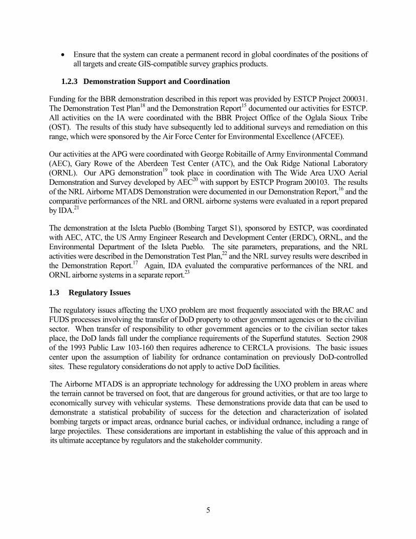
Funding for the BBR demonstration described in this report was provided by ESTCP Project 200031. The Demonstration Test Plan18 and the Demonstration Report15 documented our activities for ESTCP. All activities on the IA were coordinated with the BBR Project Office of the Oglala Sioux Tribe (OST). The results of this study have subsequently led to additional surveys and remediation on this range, which were sponsored by the Air Force Center for Environmental Excellence (AFCEE).

Our activities at the APG were coordinated with George Robitaille of Army Environmental Command (AEC), Gary Rowe of the Aberdeen Test Center (ATC), and the Oak Ridge National Laboratory (ORNL). Our APG demonstration19 took place in coordination with The Wide Area UXO Aerial Demonstration and Survey developed by AEC20 with support by ESTCP Program 200103. The results of the NRL Airborne MTADS Demonstration were documented in our Demonstration Report,16 and the comparative performances of the NRL and ORNL airborne systems were evaluated in a report prepared by IDA.21

The demonstration at the Isleta Pueblo (Bombing Target S1), sponsored by ESTCP, was coordinated with AEC, ATC, the US Army Engineer Research and Development Center (ERDC), ORNL, and the Environmental Department of the Isleta Pueblo. The site parameters, preparations, and the NRL activities were described in the Demonstration Test Plan,22 and the NRL survey results were described in the Demonstration Report.17 Again, IDA evaluated the comparative performances of the NRL and ORNL airborne systems in a separate report.23

1.3 Regulatory Issues

The regulatory issues affecting the UXO problem are most frequently associated with the BRAC and FUDS processes involving the transfer of DoD property to other government agencies or to the civilian sector. When transfer of responsibility to other government agencies or to the civilian sector takes place, the DoD lands fall under the compliance requirements of the Superfund statutes. Section 2908 of the 1993 Public Law 103-160 then requires adherence to CERCLA provisions. The basic issues center upon the assumption of liability for ordnance contamination on previously DoD-controlled sites. These regulatory considerations do not apply to active DoD facilities.

The Airborne MTADS is an appropriate technology for addressing the UXO problem in areas where the terrain cannot be traversed on foot, that are dangerous for ground activities, or that are too large to economically survey with vehicular systems. These demonstrations provide data that can be used to demonstrate a statistical probability of success for the detection and characterization of isolated bombing targets or impact areas, ordnance burial caches, or individual ordnance, including a range of large projectiles. These considerations are important in establishing the value of this approach and in its ultimate acceptance by regulators and the stakeholder community.

6

Even within active ranges, such as at the APG, environmental concerns must be addressed because soil and groundwater contamination by energetic residues and byproducts, and by heavy metals (As, Bi, Pb, Sb, U, etc.) associated with ordnance components, may migrate to underground aquifers and routinely, through run-off, reach other properties. Specifically at the APG, extensive (on base) wetlands are used by migratory birds and other waterfowl; and marine estuaries and bays beyond the APG boundaries (with known UXO contamination) are continually harvested for finfish and shellfish by both private and commercial fishermen.

Conducting UXO geophysical surveys in shallow-water wetlands and in shallow offshore areas is extremely difficult, expensive, and inefficient. The Airborne MTADS provides a technology appropriate for addressing some of these challenges. These demonstrations enabled us to evaluate the extent to which it can be applied in terrains that cannot be traversed on foot and in areas that are dangerous for routine ground activities.

7

2. Technology Description

2.1 Technology Development and Application

2.1.1 System Specifications and Requirements

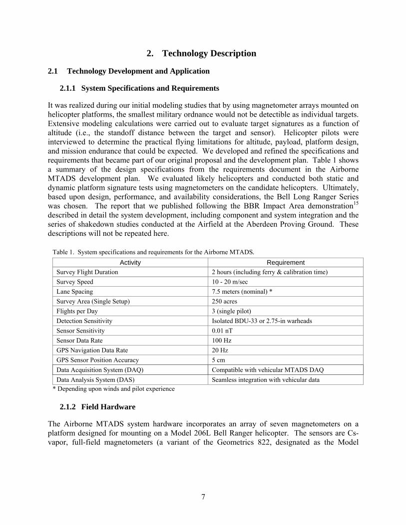
It was realized during our initial modeling studies that by using magnetometer arrays mounted on helicopter platforms, the smallest military ordnance would not be detectible as individual targets. Extensive modeling calculations were carried out to evaluate target signatures as a function of altitude (i.e., the standoff distance between the target and sensor). Helicopter pilots were interviewed to determine the practical flying limitations for altitude, payload, platform design, and mission endurance that could be expected. We developed and refined the specifications and requirements that became part of our original proposal and the development plan. Table 1 shows a summary of the design specifications from the requirements document in the Airborne MTADS development plan. We evaluated likely helicopters and conducted both static and dynamic platform signature tests using magnetometers on the candidate helicopters. Ultimately, based upon design, performance, and availability considerations, the Bell Long Ranger Series was chosen. The report that we published following the BBR Impact Area demonstration15 described in detail the system development, including component and system integration and the series of shakedown studies conducted at the Airfield at the Aberdeen Proving Ground. These descriptions will not be repeated here.

2.1.2 Field Hardware

The Airborne MTADS system hardware incorporates an array of seven magnetometers on a platform designed for mounting on a Model 206L Bell Ranger helicopter. The sensors are Cs-vapor, full-field magnetometers (a variant of the Geometrics 822, designated as the Model

Table 1. System specifications and requirements for the Airborne MTADS. Activity Requirement

Survey Flight Duration 2 hours (including ferry & calibration time) Survey Speed 10 - 20 m/sec Lane Spacing 7.5 meters (nominal) * Survey Area (Single Setup) 250 acres Flights per Day 3 (single pilot) Detection Sensitivity Isolated BDU-33 or 2.75-in warheads Sensor Sensitivity 0.01 nT Sensor Data Rate 100 Hz GPS Navigation Data Rate 20 Hz GPS Sensor Position Accuracy 5 cm Data Acquisition System (DAQ) Compatible with vehicular MTADS DAQ Data Analysis System (DAS) Seamless integration with vehicular data

* Depending upon winds and pilot experience

8

822A). The specially selected magnetometers, which are airborne quality, were acceptance tested at the manufacturer’s facility to verify sensitivity, sensor noise, heading error, dead zones, inter-sensor compatibility, and performance with the multi-sensor–interface electronics. The helicopter with the mounted magnetometer array is shown in Figures 1 and 2. All sensors are interfaced to the data acquisition system (DAQ) computer. The DAQ electronics are contained in a rack mounted in the rear starboard seat position in the helicopter, Figure 3. The power distribution interface is also in the rack, as are readouts for all the sensor inputs. The interface accepts the helicopter power (50 amps at 28 volts is available, we use ~20A) and converts it as required for the various sensors and DAQ electronics. An operator in the rear port seat monitors the survey progress. On the 9-meter boom, the seven sensors are mounted with a 1.5-meter horizontal spacing. The time-dependence of the Earth’s background field is measured by an eighth magnetometer deployed at a static surface site during a survey. The sensor positions over the

Figure 1 – Airborne MTADS survey hardware is shown being installed on a Bell Long Ranger at the Helicopter Transport Services hangar.

Figure 2 – Airborne MTADS survey on the Active Recovery Field. Note the 2-meter high vegetation that stretches from this point to the shoreline.

Figure 3 – The DAQ console is shown mounted in the rear starboard seat position. Note the Trimble Model MS-750 units mounted on the left side of the rack.

9

surface of the Earth (latitude, longitude, and height above ellipsoid) are determined using satellite-based GPS navigation, employing the latest real time kinematic (RTK) technology, which provides a real-time position update (at 20 Hz) with an accuracy in the horizontal plane of about 5 cm. Inaccuracies in the height above ellipsoid (HAE) typically are about twice those in the horizontal plane. GPS satellite clock time is used to time-stamp both position and sensor data information for later correlation.

Dual GPS antennas (Trimble Zephyrs), deployed on the forward horizontal boom, in addition to providing the position over ground and the height above ellipsoid positions for sensor mapping, provide boom roll and yaw attitude information for sensor location corrections. A separate inclinometer provides the pitch attitude correction, and a fluxgate gradiometer provides three-axis information that is used to derive aeromagnetic compensation corrections for the magnetometer sensor data. Laser (Optech Sentinal, Model 3100DV) and radar (Terra, Model TRA350/TRI40) altimeters mounted on fixtures attached to the rear hardpoint of the helicopter provide two independent altitude measurements to the DAQ computer. The dual altimeters were deployed because they provide complementary information when operating over water or vegetated surfaces.

As a result of studies conducted during the shakedown tests and the demonstration survey at the BBR, we decided to add an additional altimeter measurement capability to the platform. Three downward-facing acoustic sensors were added to the system: One was mounted on each of the forward-pointing yellow nipples (Figure 1) on the sensor boom, and a third was mounted adjacent to the laser and radar altimeters. These sensors, nominally read at 10 Hz, provide a much more comprehensive surface map, particularly when used in conjunction with the other altimeters.

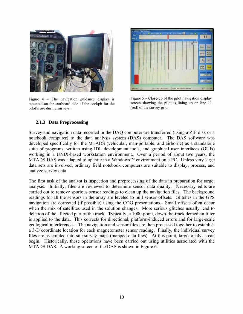
The helicopter pilot flies the survey using an onboard navigation guidance display developed specifically for this application. The sunlight-readable screen is mounted to the right of the instrument panel, Figure 4, so that it is in the field of view of the pilot without reducing his ability to visualize the whole forward boom and the field immediately ahead of the helicopter. The survey parameters are set up in this computer which shares the navigation and altimeter data with the DAQ computer.

The navigation guidance display, Figure 5, provides left-right indicators, an altitude indicator, an automatic line number increment, an adjustment for lateral offset, a color-coded flight swath overlay, and the ability to zoom the presentation scale in or out on the display. The survey course-over-ground (COG) is plotted for the pilot in real time on the display, as are presentations showing the laser altimeter data and the GPS navigation fix quality. This enables the pilot to respond rapidly to both visual cues on the ground and to the navigation guidance display. After a survey, the pilot and the analyst can isolate and survey any missed areas before leaving the site. The experience gained in the shakedown exercises was sufficient to enable surveys to be conducted without the need for additional ground support personnel.

10

2.1.3 Data Preprocessing

Survey and navigation data recorded in the DAQ computer are transferred (using a ZIP disk or a notebook computer) to the data analysis system (DAS) computer. The DAS software was developed specifically for the MTADS (vehicular, man-portable, and airborne) as a standalone suite of programs, written using IDL development tools, and graphical user interfaces (GUIs) working in a UNIX-based workstation environment. Over a period of about two years, the MTADS DAS was adapted to operate in a Windows™ environment on a PC. Unless very large data sets are involved, ordinary field notebook computers are suitable to display, process, and analyze survey data.

The first task of the analyst is inspection and preprocessing of the data in preparation for target analysis. Initially, files are reviewed to determine sensor data quality. Necessary edits are carried out to remove spurious sensor readings to clean up the navigation files. The background readings for all the sensors in the array are leveled to null sensor offsets. Glitches in the GPS navigation are corrected (if possible) using the COG presentations. Small offsets often occur when the mix of satellites used in the solution changes. More serious glitches usually lead to deletion of the affected part of the track. Typically, a 1000-point, down-the-track demedian filter is applied to the data. This corrects for directional, platform-induced errors and for large-scale geological interferences. The navigation and sensor files are then processed together to establish a 3-D coordinate location for each magnetometer sensor reading. Finally, the individual survey files are assembled into site survey maps (mapped data files). At this point, target analysis can begin. Historically, these operations have been carried out using utilities associated with the MTADS DAS. A working screen of the DAS is shown in Figure 6.

Figure 4 – The navigation guidance display ismounted on the starboard side of the cockpit for thepilot’s use during surveys.

Figure 5 – Close-up of the pilot navigation display screen showing the pilot is lining up on line 11 (red) of the survey grid.

11

In the case of relatively isolated ordnance targets, the DAS employs resident physics-based models to determine target size, position, and depth. Extensive data sets have been acquired and processed to calibrate the models. Using these models, we have demonstrated probabilities of detection approaching 100% on ranges that are not too difficult and target location accuracies of ≈15 cm with the magnetometer system.

Although we have achieved impressive results using the DAS, it has proven difficult to transition the analysis utility to the general UXO user community. After the BBR demonstration, we began performing the data preprocessing functions, through the generation of mapped data files, using a

commercial software utility, Geosoft’s Oasis montaj™. An example of a working screen from Oasis montaj™ is shown in Figure 7. The upper panel of the screen shows a portion of the Oasis database, the middle shows corrected and uncorrected plots of a segment of one of the sensor tracks, and the lower panel shows a clip of the interpolated sensor data. In a separate ongoing project at AETC,24 the MTADS target analysis algorithm is being integrated as an operational adjunct to the Oasis montaj™ suite of programs, which will enable future users of the montaj™ system to conduct physics-based target analysis using the MTADS analysis engine. More recently ESTCP has sponsored AETC to specifically adapt this development for use with airborne survey data.25

2.1.3.1 Sensor Noise The treatment of magnetometry data to correct for platform- and motion- induced signals, to a large extent, uses standard techniques. Some of these techniques have been developed and applied during the vehicular MTADS projects. These include the use of reference magnetometers to cancel diurnal field variations, a down-the-track demedian filter to cancel sensor baseline drift, sensor leveling subtractions to cancel sensor zero offset

Figure 6 – Working screen of the MTADS DAS showing the survey project view on the left and an expanded analysis window on the right.

Figure 7 – A working screen of Oasis montaj™ showing airborne data from the Isleta demonstration.

12

differences, and spatial data filtering to suppress geological effects and some platform-induced signal offsets.

2.1.3.2 Blade Noise The largest platform-induced signal is usually that associated with the rotating blades. The noise is not primarily generated by the blades themselves, but by the rotor hub assembly. These assemblies are “magnafluxed” during overhauls to inspect for stress or fatigue cracks. They are demagnetized before reinstallation, but the thoroughness of this step varies widely. The rotor noise is primarily at 6.5 Hz and 13 Hz because the helicopter is designed to operate at a constant rate (6.5 rpm). The rotor rpm rate changes significantly only if the helicopter abruptly changes attitude or altitude and quickly returns to

the nominal value. The effect is best visualized in a noise/frequency plot (power spectrum), as shown in Figure 8.

The 6.5 Hz spike varies in intensity (from ~0.3 nT to >10 nT), depending upon the helicopter. We have seen both extremes from the same machine before and after an overhaul. The 13 Hz signal reflects that the helicopter has two blades; each passes near each sensor once during a revolution of the rotor hub. The 25 Hz signal we believe is associated with a standing wave vibration of the forward sensor boom likely induced by vortex shedding or by higher frequency airframe vibrations. The 6.5 Hz and 13 Hz interference signals seen by the outboard sensors are about a factor of two weaker than that seen by the center sensor. Our typical approach is to apply narrow notch filters at 6.5 Hz, 13 Hz, and 25 Hz to suppress the noise source to nearly zero for sensors 1, 2, 6, and 7. Sensors 3, 4, and 5 often have a just-detectible 6.5 Hz signal remaining. All of these frequencies are significantly above the frequencies associated with UXO targets in field data. Applying the notch filters improves the appearance of the mapped data files and slightly improves the fit qualities for the lower intensity targets.

2.1.3.3 Platform Attitude Corrections Traditionally, in airborne geophysical surveys and military airborne search applications, a technique called aeromagnetic compensation has been used to correct for platform attitude and orientation effects in magnetometry mapping surveys. This technique, primarily used in fixed-wing aircraft, uses commercially available sensor technologies and specially developed software algorithms to reduce the platform-induced magnetic noise to levels on the order of 0.01 nT. This approach has been used in the geophysical exploration community on both fixed-wing aircraft and helicopters. Depending on the techniques used and the type of platform, the compensation has been demonstrated to reduce the

Figure 8 – An unfiltered power spectrum (left panel) is shown for sensor 6. One hour of data is included, which was taken during the survey of the Active Recovery Field. The right panel shows the same data after notch filtering to reduce blade noise.

13

platform and heading noise to 0.1-0.5 nT on some helicopters. This is well below the typical geophysical noise levels measured in our vehicular surveys due to magnetic soils and rocks and sensor motions in the spatially varying Earth’s field. The signal intensity from an individual ordnance item the size of a General Purpose (GP) bomb (or a buried UXO cache) is a few to several hundred nT, even at several meters altitude. The ability to detect and characterize an isolated large target is therefore not a matter of signal strength or signal-to-noise ratio, but a matter of having a data sampling density high enough to identify the target as a target and to characterize its magnetic anomaly signature using the dipole-fitting routine. These considerations were incorporated into the design of the horizontal sensor spacing in the array and the flying speed for the airborne platform.

NRL completed a development project with a subcontractor to adapt and apply existing aeromagnetic compensation software capabilities to the Airborne MTADS system. The subcontractor owns the rights to this program, but unlimited use rights could be purchased. The use of the algorithm involves having the aircraft fly a set of high-altitude, closed-loop maneuvers involving extremes of attitude and orientation. From these data, a set of attitude and orientation corrections is generated to compensate for the attitude-dependent, platform-induced signals. On all of our shakedown flights and during the first demonstration at the BBR, these data were taken; however, the platform attitude effects in the survey data have not warranted application of the algorithm. The urgency of the need to develop and apply these corrections has been mitigated by our success in application of the other MTADS data preprocessing techniques and filters described above. The data taken during the airborne shakedown tests and during the BBR demonstration15 have shown that our normal preprocessing steps reduce the platform-induced noise to below 1 nT. Our existing aeromagnetic compensation routines reduce extreme attitude platform effects to slightly below 1 nT. However, to prove their benefit will require that we conduct surveys on areas that are geologically quiet on the sub-nT scale. While either of these conditions is unlikely on most surveys over hard terrain, it is more likely that these corrections will be important in marine applications where a couple of meters of water exist above the bottom surface and where the bottom sediments tend to be geologically more homogeneous.

2.1.3.4 Mapping Sensor Coordinates The man-portable and vehicular MTADS platforms are designed to maintain the sensors at a fixed height (25 cm) above the ground. The optimal helicopter altitude varies considerably, depending upon the vegetation and the terrain. Therefore, the 2-D (“Flat Earth”) calculation algorithm used with the man-portable and vehicular analysis engines is inappropriate for use with the airborne data. For this reason, the analysis algorithm was upgraded to a full 3-D fitting routine. Each sensor reading is now mapped in three dimensions: an X-Y position (in Lat/Lon or UTM coordinates) and an altitude (HAE) derived from the GPS data. The GPS sensor data are time-stamped by the GPS clock that is accurate on the nanosecond time scale. The computer clock correlates the GPS pulse-per-second signal with the magnetometer trigger pulse. This is accurate at the millisecond level. The sensor coordinates are determined by applying geometric corrections relative to the primary GPS antenna position. Platform attitude corrections are derived using the secondary GPS antenna (roll and yaw) and the fluxgate and inertial attitude sensors (all attitudes).

14

Until the first demonstration at the BBR, airborne target analyses were carried out using the sensor HAE, and target tables were generated with target depths recorded in HAE. To determine the target depth below the ground surface, the surface HAE was subtracted from the target HAE. To accurately determine the surface HAE, it was measured at the time of target reacquisition. This was the approach used at the BBR demonstration.15 It was decided that this approach was unacceptable for two reasons. First, the analyst during the target fitting process needs to have an estimate of the depth to assist his decision about classifying the target as UXO or OE clutter and to determine its UXO probability. Second, the additional step to measure the surface HAE in the field during reacquisition and to calculate the target burial depth is too complex an operation to be handled by UXO technicians in the field, which leads to loss (or mis-recording) of this information unless extreme care is taken during the process. For these reasons, modifications were made both to the DAS and to the altitude measurement process. Some of these modifications are described below.

2.1.3.5 Digital Elevation Maps In 3-D surveys such as those conducted with the Airborne MTADS adjunct, the physical dimensions of the array are large and the sensor height above ground varies significantly during data acquisition. Furthermore, factors such as ground vegetation cover, reduced spatial sampling, and physical offsets of the altimeter data relative to the geophysical sensors compromise the accuracy with which we are able to measure geophysical sensor height above ground. Figure 9 schematically shows the important components of the altitude correction system.

To isolate these factors from the dipole-fitting analysis, we use the sensor HAE as the vertical reference, thereby ensuring a consistent coordinate system for both geophysical sensor input and target position output. While use of the HAE ensures a consistent frame of reference for the fitting

analysis, this measure is cumbersome for dig teams to use during the remediation process. Therefore, we derive an estimated target depth below ground surface based upon the target’s estimated HAE and a measure of the ground surface relative to this ellipsoid during the target analysis process. Data from separately positioned altimeters are used to map the ground surface and derive a Digital Elevation Model (DEM) in the same coordinate system. The depth below ground for each target can then be estimated by subtracting the target HAE from an interpolated (using the DEM) ground elevation HAE at the target’s horizontal position. In this manner, any uncertainty with respect to the measurement of the ground surface is constrained to the depth-below-ground estimate and does not compromise the validity of the feature information derived from the analysis routine itself.

Laser Altimeter

Pass 1 Datum

Pass 2 Datum

Digital Elevation Model

Ground SurfaceGround Surface

Magnetometer

GPS Antenna

WGS84 Ellipsoid

Figure 9 – Important components of the sensor boom involved in deriving the Digital Elevation Model.

15

The primary measure of aircraft height above ground level (agl) along the flight path is based upon the laser altimeter. However, using a single pass does not provide an accurate model of the ground surface under the outboard sensors because of terrain deviations lateral to the flight direction. To mitigate the sparseness of the laser altimeter data, we added three acoustic altimeters to the system. Two are located on the forward boom, in line with the GPS antennae and the magnetometer sensors, reducing the impact of pitch measurement errors and improving our lateral sample density. The third is located at the rear of the aircraft beside the laser altimeter to facilitate calibration and comparison of the acoustic altimeters relative to the laser altimeter. Figure 10 schematically shows the DEM derived using the additional elevation data. We generate a DEM of the survey area using all of the survey passes. This method effectively reduces error in our estimate of the ground surface elevation by interpolating measurements between passes, rather than assuming a uniformly level ground and extrapolating from a single pass. The DEM (based upon the input of five separate altimeters) is generated as a Geosoft “grid” file in which the survey area is broken down into a number of “grid cells,” each associated with a single value representing the interpolated ground elevation at that location. This format naturally imposes spatial filtering appropriate to the grid cell size and data sample density (when more than one sample falls within a grid cell, the resulting value is an average of the samples). A grid cell size of 1.0 m2 or less is typically used for the DEM to avoid excessive filtering along the line. After the target horizontal location estimate is derived from the dipole-fitting routine, we extract the ground surface HAE from our DEM grid at that location (using the Geosoft “grid sample” utility) and subtract it from the target HAE to derive an estimate of the target depth below ground.

Unfortunately, the acoustic altimeters have a much larger footprint; thus not only do they not penetrate well through dense vegetation but give noisy and inaccurate heights above ground in significantly vegetated areas. The usefulness of the acoustic altimeters is limited to areas with limited vegetation cover. They work very well over water or in desert environments. The DEM is created using data from the most appropriate combination of altimeter data, depending upon the site conditions. The resulting map is then used to derive HAE altitudes for each sensor reading in the survey data set.

2.1.4 Data Analysis

Currently, we can create mapped data files using either Oasis montaj™ or the MTADS DAS. For target selection and analysis, we use the MTADS DAS. We are in the process of converting the analysis routines developed under ESTCP and SERDP sponsorship to Geosoft GXs, executable

Figure 10 – Schematic of the sensor boom showing the GPS, laser, and acoustic altimeters used to derive the DEM.

16

files that can be called from the Oasis environment. Ultimately, this will enable the analyst to perform the entire data analysis from input of raw data files through data quality checks, mapping of individual sensor readings, target selection, model fit, and finally generation of target lists and output graphics entirely within the Oasis environment. All target analyses reported in this document were accomplished using routines in the MTADS DAS.

The MTADS target analysis GUI is written at multiple levels to accommodate both sophisticated and novice users. A novice user can perform data analysis using menu-driven tools and the background default analysis settings; see Figure 11. When a magnetic anomaly, such as one of those shown in Figure 11, is boxed for analysis using the computer mouse, the DAS selects the sensor data within the boxed area for consideration. Each sensor reading, with its HAE, is an input datum used in the seven-parameter iterative calculation to produce the best fit to a dipole model of the anomaly signature. Extensive training data sets (using inert ordnance) have been used to refine the algorithms to improve target analysis.

In addition to position, depth, and size solutions, magnetic analyses provide dipole orientation and effective target-caliber information and, using a “goodness of fit” analysis, provide guidance in the target-fitting process, Figure 12.

The DAS provides a range of graphical and numerical outputs to document the results of the target analysis process and to support remediation efforts. Visual images of selected parts of a survey in a variety of color and gray-scale presentations can be created showing target data overlain by landmark information and analysis results in bitmap (.tif) or editable (.ps) format. Local, State Plane, or Global Coordinate System (UTM or Lat/Lon) presentations are selectable. The graphics are appropriate either for reports or to support target way pointing and remediation operations. Numerical target analysis results are prepared in tabular form in any desired combination of coordinate systems. These outputs are formatted for incorporation into reports or for import into spreadsheets that can be electronically loaded into the GPS navigation equipment to reacquire the targets in the field in preparation for remediation.

Figure 11 – Site view and data analysis screens from the MTADS data analysis program. A part of the Mine, Grenade, and Direct-Fire Weapons Range survey is shown on the left. An individual target is boxed for analysis on the right.

17

2.2 Previous Testing of the Technology

The Airborne MTADS system was extensively tested and improved as the result of the three shakedown tests that were conducted at the Aberdeen Proving Ground. For further information, see “Technology Demonstration Plan: Airborne MTADS Demonstration on the Impact Area of the Badlands Bombing Range.”18

2.3 Factors Affecting Cost and Performance

The largest single factor affecting the Airborne MTADS survey costs and production rates is the cost of operating the survey helicopter on site. During recent surveys, charter costs have been approximately $700 per hour with a guaranteed four-hour daily minimum. Mobilization of the aircraft to and from the site, originating from its home base, is charged at the hourly charter rate. To maximize production and minimize cost, surveys should be arranged with long survey lines to minimize the time spent in turns. Frequent examination of data quality minimizes time spent taking unusable data. Minimizing time lost in refueling aircraft by having fuel available on site and basing aircraft strategically to minimize daily ferry trips to and from the survey site can represent large increases in production and decreases in cost.

The take-home message from our demonstrations is that it is unlikely to be economical to undertake Airborne MTADS surveys of less than a few hundred acres. Mitigating circumstances occur when UXO surveys must be done over water, in marshy wetlands, or in other areas where one can neither walk nor drive. In these situations, performance issues may override cost issues.

Other steps to maximize productivity for the Airborne MTADS survey of the target ranges were taken at the BBR, APG, and Isleta demonstrations:

• At APG, permission was obtained from Bell Helicopter to allow the helicopter to refuel with JP-8 (the military equivalent to Jet A).19 This was the only fuel available at the APG Airfield. Refueling with JP-8 therefore required no ferry time. Refueling took place either between survey sites or when downloading survey data for inspection.

• At APG, the helicopter was chartered from Helicopter Transport Services from their Fixed Base Operator (FBO) hangar at Martin State Airport (approximately 20 minutes’

Figure 12 – The target fit window from the MTADS DAS. Data from the target boxed in Figure 11 are shown on the left. The dipole model fit is shown on the right. Fit parameters are shown in the left and center columns. Advanced processing options are indicated in the right column, where the analyst’s comments are also recorded.

18

flying time from APG).16 The platform and electronics were assembled and mounted on the helicopter at Martin State Airport. Spares were stationed on site to provide quick recovery, if necessary.

• At all demonstration sites, one-hour missions were flown and the resulting data provided to analysts on the ground for inspection.

• At all three demonstration sites, survey missions were set up in advance on the DAQ computer. This enabled us to switch between survey sites, as necessitated by weather or logistics (e.g., sharing survey ranges with the other demonstrators), by simply starting new survey files.

• At the Isleta demonstration, a long ferry was required to bring the helicopter to the area. Rather than basing the helicopter at the Albuquerque airport, we based it at a small municipal airport nearer the target range to decrease daily ferry time to and from the site.17 A fuel tanker truck was chartered and placed on the impact range for refueling.

• All surveys were planned to start at sunup (or when weather allowed access) and end at sundown each day, with brief pilot rest breaks each hour and a 45-minute break for lunch.

2.4 Advantages and Limitations of the Technology

Unlike the vehicular magnetometer system, the airborne system is not capable of detecting the smallest classes of buried UXO at depth. While the magnetic signals are spatially spread and diminished in intensity with the sensors farther above the ground, our extensive modeling results indicated that, at an altitude of 2 meters above the ground, the system should be capable of detecting BDU-33s or Mk 82s in all geologies and ordnance targets equivalent to or larger than 2.75-in warheads in geologically quiet areas. This has generally been borne out by the demonstrations described in this report. At the geologically quiet and topologically flat prove-out site at the APG Airfield, we were able to efficiently detect both 60-mm and 81-mm mortars.16,22 At the much more highly cluttered and geologically active Isleta range, in areas with rough ground surface or significant vegetation, we failed to detect several 105-mm projectiles.17,23

The extent to which spreading target signatures interfere with each other and are obscured by geological features was carefully evaluated in the first airborne demonstration at the BBR.15 In that study, with relative large UXO targets (105-mm to 8-in projectiles) relatively sparsely distributed on the site, detection efficiency for individual UXO was equivalent for the airborne and vehicular towed arrays. Because of the lower data density and the more widely spread anomaly signatures, it proved more difficult to discriminate between UXO and clutter signatures from the airborne data than from the vehicular data. At some APG sites,16 and at the Isleta site, significantly more targets would have to be dug behind an airborne survey than behind a corresponding vehicular survey. This results from the much higher target densities and the more complex mix of UXO threats on some of these ranges that result in merging and overlapping of adjacent target signatures. The cost tradeoffs between digging more targets and reduced survey

19

production costs are (and will always be) site specific, depending upon the types of UXO challenges, the relative density of targets, geological and topological conditions, and the size of the survey site.

On open ranges, the vehicular MTADS is a relatively efficient survey technology. A survey with the magnetometer array typically achieves a production rate of 20 acres per day, while the EM array can typically survey 12-15 acres under similar conditions. When a site has vegetation cover or topography that precludes vehicular traffic, the man-portable adjunct MTADS can often be used. However, there are sites that cannot be traversed on foot, others that are dangerous, and still others that contain isolated bombing targets or impact ranges, located, at best imprecisely, within tens or hundreds of thousands of acres. For these sites, the Airborne MTADS produces much more rapid and efficient surveying, with the commensurate economic benefits. On a large site, such as the Impact Area of the BBR surveyed during the first demonstration, the Airborne MTADS routinely completed 350-500 acres per day using a two-man field crew.

The helicopter platform is designed to be flown at a low altitude (1-2 meters), with a horizontal sensor spacing of 1.5 meters and a forward velocity of 20 meters per second. To achieve this, the sensors have been fixed to hardpoints on the helicopter. As seen in Figure 1, the sensor boom extends well in front of, and is clearly and completely visible to, the pilot. This is critically important during low-altitude flights to enable the pilot to maintain minimal terrain clearance. With the sensor spacing of 1.5 meters, a data collection rate of 100 Hz, and a speed over ground of 20 m/sec, the data density is high enough to provide 30-50 data points over small targets (e.g., an 81-mm mortar) or several hundred data points for targets such as 155-mm projectiles or GP bombs. This is more than sufficient to generate high-confidence, dipole-signature fits for the individual UXO challenges.

20

21

3. BBR Demonstration

3.1 Performance Objectives

3.1.1 BBR Demonstration Objectives

The objectives of this demonstration are enumerated below:

• Prepare a 10-acre area seeded with 25 ordnance items whose locations were unknown to the survey team. Survey the seeded area and an additional 100 acres with the vehicular magnetometer MTADS array.

• Complete an extended site survey that includes both the seeded area, the additional 100-acre prove-out area, and other accessible parts of the IA using the Airborne MTADS. The airborne survey was planned to cover about 1,700 of the 2,400-acre IA. The areas along the White River and in the northern part of the IA do not lie on Bouquet Table, and were considered as unlikely UXO impact areas.

• Based upon on-site target analysis of the airborne data, use a UXO-certified recovery team to dig from the seeded area all targets on the survey dig list.

• Based upon on-site target analysis of the entire airborne survey data, dig all targets from the 100-acre survey dig list.

• Based upon the dig list prepared from the airborne survey of the remaining area, dig targets from the area surveyed only by the airborne system, beginning with the highest priority and continuing until funds are exhausted.

• Provide graphical survey products to the BBR Project Office of the Oglala Sioux Tribe (OST).

• Prepare a report15 of our activities, which includes a description of all dug targets, a listing of the positions and descriptions of all targets observed in the survey that were not dug, and an evaluation of the airborne system’s performance.

Our activities on site were coordinated to address the objectives of both this demonstration of the Airborne MTADS (ESTCP Project 200031) and the Advanced MTADS Classification Demonstration26,27 using the vehicular magnetometry and EM arrays. Each project shared information resulting from magnetometry surveys of the 10-acre area seeded with 25 inert projectiles. The extended vehicular magnetometry survey (100 acres) provided a database of survey information that was used to evaluate the performance of the airborne system over the same survey area. This comparative study was used to make refinements in the airborne data processing parameters before the final airborne target analysis and preparation of the dig lists for the entire Impact Area (IA).

22

This survey of the BBR IA is large enough to support development of production and survey cost information. From this information, we can compare the operational and production efficiencies of the vehicular and airborne systems. Complete target remediation of the 100-acre common survey area also provides statistics about the relative abilities of the two approaches to distinguish ordnance from clutter targets. If many more false alarms must be dug behind an airborne survey than behind a vehicular survey, part (or all) of the cost advantages of the airborne survey could be lost.

3.2 Selection of the Demonstration Site

MTADS demonstration projects during the period 1996-2001 were sponsored primarily by ESTCP and the Army Corps of Engineers3,4 (CEHNC). With the exception of a study of UXO contamination on the beach at the former Fort Pierce Naval Amphibious Training Base,3 the MTADS demonstrations have focused on ranges impacted by bombing and aerial gunnery training exercises. In 1999, we conducted a vehicular MTADS survey of the IA at the BBR.17 In preparation for that project, NRL conducted site visits, archival records searches, OST coordination activities, acquisition of aerial photography, and pre-surveying of first-order control points to support the survey. This earlier survey also supports the subsequent demonstrations.

In September 2001, we returned to the same area to complete the Advanced MTADS Classification Demonstration with the vehicular MTADS and to conduct the first demonstration of the Airborne MTADS adjunct platform. In support of both of these ESTCP project demonstrations, a 10-acre site was seeded with 25 degaussed targets (five 8-in, ten 155-mm, and ten 105-mm projectiles). This area was surveyed with the EM vehicular MTADS array. Subsequently, this site and an additional 100 acres were surveyed with the vehicular MTADS magnetometer array prior to beginning the Airborne MTADS survey.

3.3 Test Site History and Characteristics

3.3.1 Site and Facility History

In 1942, the Department of War annexed 341,725 acres of the Pine Ridge Reservation for use as an aerial gunnery and bombing range. This site is located in the southwest corner of South Dakota, with the largest part of the Bombing Range located in Shannon County. From 1942 until 1948, various sections of this range were used for bombing exercises and various air-to-ground operations. Since 1960, portions of the land have been returned to the OST in a stepwise fashion. In 1968, Congress enacted Public Law 90-468, returning 202,357 acres to the OST and setting aside 136,882 acres of formerly held OST lands to form the Badlands National Monument, to be managed by the National Park Service. In 1978, all remaining BBR lands were declared excess federal property with the exception of 2,486 acres (subsequently referred to as the Air Force Retained Area or the Impact Area). In about 1965, the South Dakota National Guard placed as many as 100 car bodies on the 2,486-acre area and began using them as ground-to-ground artillery targets during training exercises. The National Guard training exercises took place on the IA between 1966 and 1973.

23

3.3.2 Site and Facility Maps and Photographs

Figure 13 shows the perimeter of the Impact Area in red. The 2500-acre IA is surrounded by a buffer zone, generally of about 1,000-m width. The IA buffer boundary fence, outside the IA, is shown in green. The most direct access to the IA is by a dirt road that exits to the south from State Highway 40. There is only one fence internal to the IA. This east-west fence bisects Sections 29 and 30 and is labeled “Cross Fence” in Figure 13.

Three geodetic survey points are located on the IA. Ellsworth AFB CES (civil engineering) personnel, using the OST 5 benchmark (not shown in Figure 13), upgraded these sites, labeled North BM, East BM, and USGS BM, to “near first-order.” NRL contractors established the OST 5 point in 1997; it is legitimately first order.7 All 1999 NRL surveys were done using the North BM coordinates as provided by Ellsworth AFB. The coordinates of each of these points are given in Table 2 below. The black inset in Figure 13 contains the 100-acre 1999 MTADS survey area, which is shown in green. Excavation of targets in the 100-acre area led to recovery of five 8-in and ten 155-mm HE-filled and fuzed projectiles. These projectiles were fairly evenly distributed across the survey area. The location of the bull’s eye, which is more clearly seen in Figure 14, is just southeast of the crossroads.

3.4 Previous UXO Clearances

There have been six UXO clearance operations carried out on the BBR between 1948 and 1997. These are discussed in more detail in Ref. 28. Only two have significant relevance to the present demonstration on the IA. No record of air-to-ground bombing exists that specifies the IA as a target range.

3.4.1 The 1975 Clearance

During the summer and fall of 1975, 10 EOD personnel participated in a walking search line clearance of 22,403 acres and a vehicular search of 19,222 acres. This included a walking search line survey of the entire IA and the buffer zone. With the exception of the IA, all lands were declared as cleared and certified for return to the OST. The IA reportedly contained too much ordnance and explosive (OE) material to declare the area “cleared.” The 1975 Certificate of Clearance describes the plowing of 1,088 acres of the IA using ripper plows to clear buried ordnance. Aerial photographs clearly show that the plowing took place after 24 July 1976.28

Table 2. Impact Area survey coordinates provided by Ellsworth AFB. Northing

(m) Easting

(m) Point Latitude Longitude NAD 83

Altitude (HAE m)

OST 5 43o 42' 05.2702" -102o 18' 35.5186" 4842233.05 716761.31 804.460 North BM 43o 40' 19.1197" -102o 14' 20.5113" 4839145.82 722578.26 762.530 East BM 43o 39' 21.2053" -102o 13' 42.8268" 4837387.20 723481.89 764.260

USGS BM 43o 38' 53.7820" -102o 14' 18.7564" 4836514.29 722705.23 765.940

24

Figure 13 – The BBR Impact Area lies within the red boundary. The 1999 survey area is shown in green. The 10-acre seed target area, bounded by a thinner red border, lies within this area.

25

Figure 14 – Plot of the area surveyed using the vehicular MTADS in 1999 is shown in green. The seeded target area for the 2001 demonstration was mostly surveyed and dug during the 1999 survey.

26

The clearance report documents recovery of the items listed below without specifying which, if any, of these items were associated with the IA:

• 5 – 155-mm Howitzer projectiles

• 3 – 155-mm illumination projectiles

• 1 – 8-in Howitzer projectile

• 1 – 10-lb spotting charge

• 2 – 155-mm illumination candles

• 4 – smoke grenades

• 15 – 50-caliber cartridges

• 46 – 100-lb practice bombs

3.4.2 The 1997 Clearance

During the four-month summer period, a walking and driving search line ordnance clearance was conducted by 20 EOD personnel operating from Ellsworth AFB. With the exception of 56 acres of rugged terrain along the escarpment above the White River, the entire IA was covered. EOD teams used metal detectors (mine detectors) to search for buried metal. The objective was to clear the area to a depth of 1.5 feet. The OE scrap recovered included 4,000 lbs of shrapnel (pieces larger than 3 inches). An additional 8,000 lbs of non-ordnance related metal scrap was recovered, including 6 car bodies, a washing machine, and barbed wire and fencing material. The 1997 UXO clearance documented the presence and recovery of the ordnance listed in Table 3. The 20-mm and 50-cal rounds were unfired and were likely accidentally released on the site and are not indicative of ordnance expended on the range.28

Table 3. Recovered and documented ordnance items from the IA in the 1997 clearance.

Ordnance Size Fill Comment M 106 Howitzer Projectile 8 in 36.6 lbs TNT M 107 Howitzer Projectile 155 mm 14.6 lbs TNT

Illumination Projectile 155 mm Mg Powder/NaNO3 M 1 Howitzer Projectile 105 mm Composition B

Projectile 20 mm Incidental Release from Aircraft Gun Clearances

Ammunition 50 caliber Incidental, from Small Arms Practice

27

3.5 Testing and Evaluation Plan

3.5.1 Demonstration Setup and Operation

Primary support for the MTADS demonstration on the IA was provided by the ESTCP. Oversight of the NRL activities on the IA was provided by the Environmental Office (Civ 28 CES/CEVR) of Ellsworth AFB. All operations associated with this demonstration were coordinated with the ESTCP Program Office, CENWO, Ellsworth AFB, EPA (Region 8), the South Dakota Department of Environment and Natural Resources, and the Badlands Bombing Range Project Office of the OST. The specific operations are described in the demonstration test plan,18 which was approved by the ESTCP Program Office.

NRL, Code 6110, was the manager for all activities associated with the Airborne MTADS demonstration on the IA. The NRL on-site project manager, J.R. McDonald, was responsible for coordinating operations at the IA and approving alterations or changes to the demonstration plan or schedule. All persons working on site were NRL employees, contractors working for NRL, or were employees or subcontractors of the prime contractors. There was a safety officer present at all times on site who was the authority for decisions on safety-related issues. The Senior UXO Supervisor was the safety officer for UXO digging operations. On each day that surveying or digging operations were conducted, tailgate site safety briefings were conducted before fieldwork began. Separate safety briefings were conducted for UXO personnel and the survey crews.

3.5.1.1 The Seed Target Area APG degaussed inert ordnance to prepare the seed target area. The ordnance was shipped to ERDC in Vicksburg, MS and was transported from there to the IA in South Dakota where the 10-acre seeded site was prepared during August 2001. NRL defined the corners of the test site and provided the coordinates to ERDC. The boundary of the 10-acre (200 m × 200 m) area is indicated by the red outline in Figure 14. The 10 acres fall primarily in an area that was surveyed in 1999 using the vehicular magnetometer array and was subsequently remediated to remove targets that were potentially 105-mm, 155-mm, or 8-in projectiles. Since the area is only 100-300 meters away from the center of the bull’s eye, there is a relatively high density of shrapnel and clutter (remains of automobile body parts) present on the site. The inert UXO targets were emplaced using an auger that bored slanting holes so that there were no surface scars directly above the UXO. The ground truth for the site was held by ERDC until after the magnetometry analyses from both the vehicular and airborne surveys had been submitted to ESTCP and ERDC. The ground truth for the seeded projectiles is provided in Table 4.

3.5.1.2 Logistics Because of the complexity of the simultaneous parallel airborne demonstration and the Advanced Classification Demonstration, it was important that the logistics support be carefully planned and coordinated. The logistics facilities served as a focal point for all field activities. The location of the MTADS data analysis equipment in a separate trailer provided the base station for communications and a contact point for site visitors. The second trailer provided the depot for equipment storage and repair.

28

No support services were available on site. The nearest source for rental equipment was Rapid City, about 75 miles away. Figure 15 shows some of the logistics support equipment that was set up for the demonstration. The left-most trailer served as the command center. All computers supporting data analysis were housed there. The next trailer provided storage for the hardware and housed all the battery-charging stations. The third trailer was the site office for the OST workers and, during the excavation operations, also for the UXO teams. The fourth trailer, which opened at both ends, served as a drive-through garage for the vehicular systems. Between the fourth trailer and the tractor-trailer, a tent cover was set up to provide protection for working on the vehicles or other equipment. The tractor-trailer was used to transport the vehicular equipment and the airborne sensor platform to the site. The truck at the south end was the Jet A tanker for the helicopter. To the east of this equipment were located portable toilets, a 65 kw

Table 4. Ground truth table for the inert seed ordnance emplaced at the Impact Area.

Item # Northing (m) Easting (m) Depth (m) Azi. (deg) Incl.

(deg) Nose U/D

Serial No.

8-inch 1-2 4838171.34 722824.74 0.75 350 75 D 4 1-4 4838142.67 722957.56 0.50 270 45 D 5 1-6 4838117.82 722874.46 0.75 40 80 D 3 1-8 4838082.55 722834.30 0.30 10 0 H 6 1-10 4838019.39 722889.76 0.50 340 40 D 2 155-mm 1-12 4838120.88 722786.50 0.85 0 45 D 10 1-14 4838086.48 722802.76 0.25 250 65 D 8 1-16 4838176.31 722813.27 0.60 15 80 D 12 1-18 4838143.69 722819.03 0.85 115 45 D 11 1-20 4838066.32 722848.56 0.25 165 70 D 13 1-22 4838142.69 722860.13 0.25 110 0 H 15 1-24 4838168.67 722886.90 0.30 360 35 D 9 1-26 4838106.46 722901.24 0.55 75 45 U 14 1-28 4838202.03 722921.32 0.60 30 40 D 6 1-30 4838137.07 722919.42 0.40 310 55 D 7 105-mm 1-32 4838196.19 722853.42 0.25 110 35 D 16 1-34 4838176.23 722831.42 0.92 05 75 D 9 1-36 4838174.21 722879.23 0.40 115 45 D 10 1-38 4838164.65 722931.82 0.25 30 0 H 7 1-40 4838141.72 722893.58 0.50 50 55 D 13 1-42 4838118.78 722830.47 0.60 245 75 U 15 1-44 4838070.04 722926.09 0.50 65 60 D 12 1-46 4838064.41 722957.64 0.25 315 80 D 11 1-48 4838050.93 722914.61 0.30 25 35 D 8 1-50 4838032.77 722808.48 0.30 360 45 D 14 Corners NW 4838214.74 722778.78 NE 4838214.73 722978.77 SE 4838014.77 722978.76 SW 4838014.73 722778.79

29

Figure 15 – Logistics setup supporting the demonstration at the Impact Area.

generator, and a diesel storage tank. Not shown in the image are the two four-wheel-drive backhoes that supported the UXO excavation work.

3.5.1.3 On-Site Support Two NRL employees were on site at all times during operations. Dr. J.R. McDonald was the principal investigator (P.I.) and on-site manager for the Airborne Demonstration Project. Dr. H.H. Nelson was the P.I. and on-site manager for the Advanced UXO Classification Demonstration. Nova Research, Inc. (Nova), coordinated all rentals and leases for on-site equipment. The site safety officer was an EOD-certified Nova employee who also had responsibility for site hardware maintenance and vehicle operation. The Army Research Laboratory (Blossom Point Detachment) provided the driver for the tractor-trailer that transported the MTADS equipment between Blossom Point and the Impact Area in South Dakota. AETC Incorporated supported the demonstrations with 5 on-site employees. They supported the data handling and processing for both projects. Additionally, they supported the Advanced UXO Classification Demonstration’s field activities, managed flight operations for the airborne survey, and supported data analysis and creation of survey documentation. Helicopter Transport Services, Inc., provided the helicopter and pilot for the airborne survey.

Vehicular survey operations were supported by 3-5 OST members from the BBR Project Office. Additionally, two EOD technicians from the BBR Project Office supported the dig teams. All target way pointing and recovery operations were the responsibility of Explosive Ordnance Technology, Inc. (EOTI). The 4-person EOTI staff, with support of the certified OST technicians, were formed into two dig teams. These teams conducted all target recovery operations, recorded the results of each dig on the dig sheets, photographed the recovered objects from each hole, and refilled and tamped each hole, returning it to grade. In addition, EOTI had the responsibility of providing explosives and blowing in place all recovered ordnance. All recovered OE scrap (and other metal scrap) was certified as explosives-free and stockpiled for disposal by Ellsworth AFB.

3.5.1.4 Demonstration Activity The airborne platform spare assemblies were shipped by motor freight for storage at the Rapid City Regional Airport. Since they were not needed, they remained at the airport until the end of September and were returned to NRL by motor freight. All the other equipment was shipped in a 53-foot trailer that left Blossom Point on 31 August for the Impact Area. A Nova employee arrived at the IA the week of 3 September to oversee the placement of the logistics support rental equipment. The activity log in Table 5 provides information describing the field activities of each of the project demonstrations. The

30

equipment difficulties with the EM sensors required adjusting the schedules for the vehicular survey operations to allow for repairs and recalibration of the EM array.

Table 5. Activity log for the demonstration projects on the IA.

Date Activity Result Comment

5-Sep Logistics support All components in place Electrical wiring complete

6-Sep Trailer truck arrives on site Backhoe used to repair road

7-Sep MTADS Components Unpacked & Assembled

9-Sep NRL & Support contractors arrive

10-Sep Coordinate OST and contractor activities Set up data analysis trailer & prepare for EM vehicular survey

EM 61 Mk II calibration tests, hardware failure, equipment shipped to Canada for repair

11, 12 Sep Begin vehicle mag survey of South & Seed Target Areas

Survey 200 X 600 m area, including the Seed Target Area 11 data files, 9.6 survey hours

12-14 Sep Begin vehicle mag survey of north area Survey 325 X 400 m area 13 data files, 10.0 survey hours

14, 15 Sep Begin vehicle mag survey of west area Survey 525 X 325 m area 14 data files, 11.3 survey hours

17-Sep Vehicle mag survey analysis, South, Seed, North, & West Areas

Completed target analysis & prepared spreadsheets

17-Sep Deploy EM61 Mk I Center sensor failed calibration Shipped sensor to Canada for repair

18-Sep Deploy EM61 Mk I on Seed Target Area Survey without center sensor 3 data files, 1.61 survey hours

19-Sep Deploy EM61 Mk II following repairs Perform calibration tests

20-Sep Deploy EM61 Mk II on Seed Target Area Complete N/S survey 11 data files, 6.3 survey hours, repaired EM61 Mk I received

21-Sep Deploy EM61 Mk II on Seed Target Area Complete E/W survey 14 data files, 6.8 survey hours

22-Sep Deploy EM61 Mk I on Seed Target Area Complete E/W survey 8 data files, 6.0 survey hours

22-Sep Assemble airborne components Helo arrives on site

23-Sep Deploy EM61 Mk I on Seed Target Area Complete N/S Survey 8 data files, 7.0 survey hours

23-Sep Install platform on helo Conduct practice survey of North Area

1 Data File, 1.1 survey hours, GPS data defective

23-Sep Airborne Survey of South and Seed Areas 1 Data File, 0.9 survey hour

24-Sep Deploy EM61 Mk I on Seed Target Area containing 60- & 81-mm

Survey 50 X 200 m area, complete E/W survey 3 data files, 1.61 survey hours

24-Sep Airborne Platform Repairs Replace GPS Antennas & Mag Sensor 5 and Cables

25-Sep Airborne Surveys, Airborne South Sorties

Sortie South 12, Sortie South 1, Sortie South 0, Sortie South 11, Sortie South 5, Sortie South 6,

16 Acres, 0.4 Survey Hours, 107 Acres, 1.5 Survey Hours, 107 Acres, 2.0 Survey Hours, 26 Acres, 0.5 Survey Hours, 88 Acres, 1.1 Survey Hours, 78 Acres, 0.9 Survey Hours, 68 Acres, 0.9 Survey Hours, 34 Acres, 0.6 Survey Hours

31

Table 5. Continued.

Date Activity Result Comment

25-Sep Analysis of Airborne South/Seed Data Completed Joint Target Analysis of South Seed Area

Submitted Seed Dig Lists to ESTCP and ERDC

26-Sep Airborne surveys, Airborne South & North sorties

Sortie South 8, Sortie South 9 (data lost), Sortie South 10, Sortie South 13, Sortie South 10, reflight Sortie North 1.

23 acres, 0.4 survey hour, 47 acres, 0.7 survey hour, 37 acres, 0.6 survey hour, 5 acres, 0.1 survey hour, 37 acres, 0.7 survey hour, 93 acres, 1.3 survey hours, 87 acres, 1.5 survey hours, 91 acres, 1.2 survey hours, 47 acres, 0.7 survey hour.

27-Sep Airborne surveys, reflights, and calibrations

South, missed area reflights, Sortie North 8, Sortie North 4, Sortie North 5, Upper Plateau Sortie North 6, Sortie North 5, Lower Plateau, Sortie N.

0.5 survey hour, 103 acres, 1.5 survey hours, 96 acres, 1.2 survey hours, 44 acres, 0.5 survey hour, 100 acres, 1.2 survey hours, 55 acres, 0.7 survey hour, 102 acres, 1.0 survey hour, 0.3 hour

27, 28 Sep Unmount airborne platform Helo departs

28-Sep Dig teams arrive on site Coordinate with Tribal team and analysis teams Practice target waypointing

28-Sep Airborne target analysis Analysis completed & reconciled Airborne spreadsheets & dig lists prepared

1-Oct Dig teams waypoint south & seed areas Begin recovering seed targets

?-Oct Target recovery from ground surveys All targets dug in vehicle surveyed areas Began digging airborne targets

19-23 Nov Airborne target digging terminated Final blow-in-place demolition, OE scrap sorted and certified

23-Nov Site cleaned, flags removed Dig teams depart

30-Nov All logistics support removed

The 11 September terrorist attacks in New York and Washington delayed for one week the departure of the helicopter from Baltimore to support our operations. It was uncertain until 20 September whether or not we would be able to conduct any airborne survey activities.

3.6 Results

3.6.1 Overview

The demonstration survey, analysis, and remediation activities are discussed in three sections. Initially, the vehicular and airborne surveys of the Seed Target Area, Figure 16, are presented. We compare the relative abilities of the two systems to detect the seeded ordnance and to differentiate between clutter and ordnance. There were 170 targets dug in the 10-acre area. This

32

includes all targets appearing in the vehicular magnetometer survey, the vehicular EM survey, and airborne magnetometer survey analyses.

Following discussion of the Seed Target Area, we expand our comparisons to the 100-acre area, which was jointly surveyed by the airborne and vehicular systems. In Figure 16, the 100-acre joint vehicular and airborne surveys are shown as three separate survey areas: the North, South, and West survey blocks. After independent target analyses of the two data sets, we dug all 301 analyzed targets in the area. In these 100 acres, we recovered 9 HE-filled UXO projectiles, including three 8-in and six 155-mm projectiles.

In the remaining areas surveyed by the airborne system, referred to as the Airborne Production Survey area, we analyzed 1,193 anomalies; 744 were classified as possible UXO targets. Of these, 527 were dug, and an additional six 155-mm and four 8-in HE-filled dud projectiles were recovered. This left 656 analyzed, but unrecovered, targets on the dig lists. The overall performance of the airborne survey system is then evaluated and compared with the results that would have resulted from an independent vehicular survey. Following consideration of the three survey areas, we extend the discussion to consideration of airborne production rates and relative costs for the airborne system compared to vehicular surveys.

Figure 16 provides a perspective of the vehicular surveys conducted during this demonstration compared to the vehicular surveys conducted in the 1999 demonstration. Pertinent landmarks are noted. The areas surveyed with the vehicular system in the 2001 demonstration are overlaid in blue showing their relationship to the earlier surveys.

Figure 16 – Magnetic anomaly map of the areas surveyed in 1999. The vehicular survey areas covered in the 2001 demonstration are shown in blue.

33

The 2001 vehicular surveys were partitioned into three separate areas denoted as 2001 West, 2001 North, and 2001 South. The 2001 South block is contiguous to the 10-acre Seed Target Area. The Seed Target Area was extended in this way to create the Seed-South survey block because the longer east-west lanes were more efficient to survey with both the vehicle and the airborne systems. The Seed Target Area lies 100-300 m (SE) from the center of the bull’s eye and is therefore fairly densely populated with shrapnel and clutter objects left behind following the 1999 remediation. The remaining 20 acres that constitute the 2001 South survey block lie in an area that had not been previously surveyed by the MTADS.

Other than the Seed Target Area, areas surveyed in the 1999 survey were not analyzed or remediated as part of this demonstration. The bull’s eye area was not completely remediated in 1999. We prepared target lists for digging in these areas based upon the 1999 survey, but they have not been dug.

The 2001 Seed-South block was independently surveyed using the Airborne MTADS (Table 8) to provide an initial data set for comparative analysis with the vehicular data (see Section 3.6.5). The area was reflown as part of sortie South 3 (see Section 3.6.5 and Figure 19); however the data used for target analysis on the 2001 Seed-South block was from the initial mission.

3.6.2 The Seed Target Surveys

The Seed Target Area is pictorially defined in Figures 13, 14, and 16 and the corner locations are given in Table 4. Figure 17 shows magnetic anomaly images of the Seed Target Area from the vehicular and airborne surveys. Many of the inert ordnance targets are apparent. The coordinate system in these images (and all other anomaly images generated by the MTADS DAS) is a user-defined local coordinate system in meters. The origin of the local coordinate system was chosen to be identical to that used in the 1999 MTADS survey. The offset between local and UTM coordinates is recorded at the top of all target analysis spreadsheets.

There are both striking similarities and striking differences between the two images. All apparent targets in the airborne survey have counterparts in the vehicular survey. The inverse is not true. Many of the smaller clutter targets are not detected in the airborne survey. In the airborne survey, the sensors are 4-20 times more distant from the ground surface than in the vehicular survey. The primary effects of this are a significantly decreased signature intensity (note the presentation scales) and a spreading of the anomaly signature in the airborne data. Figure 18 shows (2,000 m2, ≈1/4-acre) pixel image presentations typical of those used during the target analysis process. In the vehicular survey, three targets in this area (152, 153, and 154) were chosen for analysis. They include a 105-mm, an 8-in, and a 155-mm inert projectile, each buried between 3.5 and 4.5 feet deep. Three additional targets in the area (207, 208, and 209) were chosen in the airborne survey for analysis. In the airborne analysis, the fit sizes of these targets made them possible projectiles.

34

Figure 17 – Magnetic anomaly images of the Seed Target Area from the airborne survey on the left and the vehicular survey on the right. The Seed Target Area is 200 m × 200 m; the southwest corner coordinates are X =360 m, Y = 530 m.

35

In the vehicular survey, the much higher data density reveals target 207 to be a pair of smaller targets, 208 to be a distributed clutter target, and 209 to be a cluster of smaller clutter items. In the airborne survey, the 209 target signature appears heterogeneous, as is reflected in the fit quality. It was categorized as likely not ordnance; however, it remained above the dig threshold given our current limited experience with airborne data.

The vehicular analysis was carried out first. In this analysis, we categorized 55 targets as 105-mm UXO (category 1-3), 12 targets as 155-mm UXO (category 1-3), and 5 targets as 8-in UXO (category 1-3). Based upon the test plan for the Seed Target Area, we expected that 10 105-mm, 10 155-mm, and 5 8-in inert projectiles would be buried. With the knowledge that the 105-mm targets were likely significantly over-picked, the predicted list of UXO projectiles was consistent with our expectations. No adjustments were made in our analysis of the Seed Target Area. The results were submitted to ESTCP as analyzed.

The airborne analysis was carried out with both the vehicular and airborne data displayed side by side, as shown in Figure 18. In the Seed Target Area, the airborne target picks have the same target numbers as in the vehicular survey analysis. All inert buried ordnance were detected and analyzed in both the vehicular and airborne surveys. With one exception (target 121), all inert seed targets were recommended for digging (UXO categories 1-5). In the vehicular analysis, 19 inert seed targets were classified as category 1, 5 as category 2, one as category 3, one as category 5, and one as category 6. Target number 86 was a 155-mm projectile oriented east-west. The signature of this target is completely dominated by remnant moment; it was

Figure 18 – Magnetic anomaly maps of a portion of the Seed Target Area presented in pixel format. The airborne survey is shown on the left and the vehicular survey on the right.

36

incorrectly degaussed before burial. Target 86 has a signature appropriate for a steel fence post extending well above the ground surface. Interestingly, in addition to the inert ordnance recovered in the Seed Target Area, a live HE-filled 155-mm projectile, target 104, was recovered. In 1999, this target was also detected and subsequently dug. It was described as a “155-mm base injection type HE-filled projectile, oriented SW-NE” at a depth of 0.6 m. It was presumably inadvertently left in place and the hole refilled to grade. The target was blown in place following its discovery in 2001.

In the 2001 vehicular survey of the 10-acre Seed Target Area, 170 targets were analyzed and catalogued. Seventy-five were listed as UXO: 24 in category 1, 15 in category 2, and 36 in category 3. Ninety-five were listed as “not UXO”: 3 in category 4, 37 in category 5, and 55 in category 6. When these targets were considered in the airborne survey, 23 could not be analyzed, either because there was no detectible signature, the signature was lost in an adjacent target signature, or the fit would not converge. None of these vehicular targets were UXO, and 21 of the 23 were in category 5 or 6 in the vehicular analysis. In the airborne survey, an additional 40 targets were chosen for analysis that had been excluded from the vehicular survey analysis. These targets were included in the airborne analysis because they could not be excluded based upon the shape information that was used to exclude them in the denser vehicular data; see Figure 18 and the accompanying discussion.

In the absence of the vehicular survey data, 39 of the 40 additional targets chosen in the airborne analysis would have been dug as potential UXO. This was partially offset by the 23 targets in the vehicular data set that would not have appeared in an airborne (only) survey. If these had been commercial surveys and remediation category 1-5 targets were dug (and category 6 targets were left in the field), 115 targets would have been dug behind the vehicular survey and 161 targets would have been dug behind the airborne survey. All UXO would have been recovered based upon the airborne survey and one target (121) would have been left in the field, based upon the vehicular survey and analysis. The FAR (false-alarm ratio) would have been 115/25 = 4.6 in the vehicular clearance and 161/26 = 6.2 in the airborne clearance.

Table 6 shows data relating to the inert targets in the Seed Target Area. This information enables comparisons of the performance of the airborne and vehicular arrays. Each survey approach led to selection and analysis of all the inert targets. Target 254 (an 8-in projectile) has also been included, although it was buried just north of the seed target area. The live 155-mm projectile (target 104) is also included. The vehicular magnetometer array, because it produces very-high-density sensor data, generates more accurate location predictions. The average deviation from the ground truth of 15 cm is typical. The sensor data from the airborne system has about one tenth the density of the vehicular data.

This data density is still sufficient to provide location accuracies of better than 25 cm. The ground truth data, compiled by ERDC, provide the depth to the shallowest part of the buried item. The MTADS DAS predicts the depth to the center of the target. With the exception of target 86 (large remnant moment) and target 121 (overlaid by shrapnel), all inert items are categorized as 1, 2, or 3.

37

Table 6. Vehicular and airborne survey comparisons with the ground truth in the Seed Target Area.

MTADS ID Survey UTM X(m) UTM Y(m)

Î XY (m) Vehicular

Mag

Î⎠XY (m) Airborne

Mag

Depth (m) Size (m) Moment Incl Azi Fit

Quality Analyst Comments UXO Category

G3S-13 Vehicular Mag 722,808.40 4,838,032.85 0.11 0.63 0.125 1.1133 71 261 0.952 poor degaussing?, 105, nose down 2

Airborne Mag 722808.47 4838032.75 0.02 0.34 0.135 1.4079 61 235 0.983 105/155mm 1 Ground Truth 722808.48 4838032.77 0.30 105 mm 45 360 Nose DownG3S-26 Vehicular Mag 722,889.71 4,838,018.86 0.53 1.09 0.166 2.6054 88 147 0.942 likely 155, nose down 1

Airborne Mag 722890.06 4838019.21 0.35 0.51 0.153 2.0426 67 43 0.950 155mm 1 Ground Truth 722889.76 4838019.39 0.50 8 inch 40 340 Nose DownG3S-59 Vehicular Mag 722,957.47 4,838,064.38 0.17 0.88 0.147 1.8154 82 170 0.975 good fit for a 155 1 Airborne Mag 722957.83 4838064.09 0.38 0.21 0.144 1.6945 68 154 0.949 155mm 1 Ground Truth 722957.64 4838064.41 0.25 80 315 Nose DownG3S-65 Vehicular Mag 722,914.61 4,838,051.01 0.08 0.78 0.101 0.5827 85 198 0.719 possible 105 3 Airborne Mag 722914.59 4838050.95 0.03 0.127 1.1597 67 260 0.935 105/155mm 1 Ground Truth 722914.61 4838050.93 0.30 105 mm 35 25 Nose DownG3S-86 Vehicular Mag 722,802.70 4,838,086.48 0.06 0.70 0.217 5.8345 -69 282 0.950 totally inverted, fence post? 5 Airborne Mag 722802.81 4838086.55 0.09 0.22 0.210 5.3199 -61 268 0.988 fence post 5 Ground Truth 722802.76 4838086.48 0.25 155 mm 65 250 Nose DownG3S-88 Vehicular Mag 722,848.53 4,838,066.46 0.14 0.73 0.204 4.8764 75 355 0.947 good fit for 8in 1 Airborne Mag 722848.53 4838066.12 0.20 0.51 0.215 5.6443 83 29 0.964 8 in 1 Ground Truth 722848.56 4838066.32 0.25 155 mm 70 165 Nose DownG3S-89 Vehicular Mag 722,834.26 4,838,082.69 0.15 0.73 0.192 4.0375 29 15 0.962 155mm/8in, good target 1 Airborne Mag 722834.18 4838082.60 0.13 0.14 0.185 3.6480 28 15 0.989 155/8in 1 Ground Truth 722834.30 4838082.55 0.30 8 in 0 10 FlatG3S-99 Vehicular Mag 722,926.09 4,838,070.01 0.03 0.88 0.141 1.6053 74 222 0.969 105, nose down 1 Airborne Mag 722926.01 4838069.93 0.13 0.46 0.140 1.5677 69 240 0.975 155mm 1 Ground Truth 722926.09 4838070.04 0.50 105 mm 60 65 Nose DownG3S-104 Vehicular Mag 722,958.73 4,838,109.38 0.83 0.164 2.5117 31 28 0.974 155mm 1 Airborne Mag 722958.63 4838109.24 0.90 0.156 2.1599 30 18 0.950 155mm 1

Vehicular EM 722958.81 4838109.32 0.70 0.168 15 -210 0.976 mag 104 LIVE 155mm

G3S-109 Vehicular Mag 722,901.28 4,838,106.51 0.06 1.10 0.209 5.2247 72 270 0.956 8-in, E/W 1 Airborne Mag 722901.15 4838106.79 0.34 0.49 0.196 4.2892 58 294 0.976 8 in 1 Ground Truth 722901.24 4838106.46 0.55 155 mm 45 75 Nose UpG3S-112 Vehicular Mag 722,874.50 4,838,117.74 0.09 1.34 0.225 6.5351 84 254 0.969 8-in deep 1 Airborne Mag 722874.44 4838117.79 0.03 1.13 0.242 8.1181 74 242 0.961 8 in 1 Ground Truth 722874.46 4838117.82 0.75 8 in 80 40 Nose DownG3S-118 Vehicular Mag 722,830.52 4,838,118.83 0.07 1.34 0.177 3.1792 75 65 0.918 155 deep, nose down 1 Airborne Mag 722830.60 4838118.90 0.18 0.35 0.130 1.2576 81 62 0.962 155mm 1 Ground Truth 722830.47 4838118.78 0.60 105 mm 75 245 Nose UpG3S-121 Vehicular Mag 722,786.29 4,838,121.08 0.29 0.90 0.092 0.4383 44 4 0.867 clutter 6 Airborne Mag 722786.84 4838120.64 0.42 0.35 0.094 0.4786 54 45 0.946 unlikely 105 3 Ground Truth 722786.50 4838120.88 0.85 155 mm 45 0 Nose DownG3S-127 Vehicular Mag 722,818.86 4,838,143.80 0.20 1.32 0.112 0.8004 65 329 0.910 really deep 105? 2 Airborne Mag 722818.82 4838143.58 0.23 0.63 0.104 0.6485 71 333 0.956 105mm 1 Ground Truth 722819.03 4838143.69 0.85 155 mm 45 115 Nose DownG3S-132 Vehicular Mag 722,860.18 4,838,142.72 0.06 0.55 0.132 1.3152 45 316 0.983 likely 105 1 Airborne Mag 722860.15 4838142.55 0.14 0.05 0.132 1.3232 44 309 0.972 155mm 1 Ground Truth 722860.13 4838142.69 0.25 155 mm 0 110 FlatG3S-133 Vehicular Mag 722,893.48 4,838,141.68 0.10 0.65 0.117 0.9054 55 251 0.960 105, slight remnant 2 Airborne Mag 722893.51 4838141.52 0.21 0.37 0.127 1.1689 55 248 0.912 Ground Truth 722893.58 4838141.72 0.50 105 mm 55 50 Nose DownG3S-135 Vehicular Mag 722,919.68 4,838,136.81 0.37 1.01 0.133 1.3313 69 54 0.874 105mm, nose down 1 Airborne Mag 722919.49 4838136.59 0.48 0.30 0.113 0.8177 79 66 0.961 105mm 1 Ground Truth 722919.42 4838137.07 0.40 155 mm 55 310 Nose DownG3S-139 Vehicular Mag 722,957.75 4,838,142.70 0.19 1.10 0.210 5.2659 70 84 0.981 8-in, E/W 1 Airborne Mag 722957.80 4838142.46 0.32 0.56 0.203 4.7531 62 99 0.983 8in nearly nose down 1 Ground Truth 722957.56 4838142.67 0.50 8 in 45 270 Nose Down

38

3.6.3 The South, West, and North Surveys

3.6.3.1 The South, West, and North Vehicular Surveys Figure 16 shows the relative positions of the 2001 vehicular magnetometer survey areas. Excluding the Seed Target Area, which was discussed in Section 3.6.2, the remainder of the vehicular magnetometer survey encompasses 99.6 acres (40.3 hectares). The vehicular data were analyzed immediately on site in preparation for the anticipated onslaught of airborne data once the Airborne Production Survey began. The data were processed on the 6-category priority scale described earlier. All targets (categories 1-6) analyzed in the vehicular survey were dug. Target recovery operations began on 1 October, following completion of the airborne survey. The Seed Target Area was way pointed and dug first to recover the inert ordnance, and then the remainder of the targets from the South, West, and North blocks were dug.

3.6.3.2 The South, West, and North Airborne Surveys The Seed Target Area and the South block were initially surveyed on 23 September as a single, continuous 200 m × 600 m mission in the first airborne test survey at the IA. Data from this initial 30-acre survey were used to carry out the airborne target analysis of the Seed Target Area and South block.

Target digging in the Seed Target Area was based upon the combined analyses of the vehicular magnetometer and EM and airborne magnetometer MTADS survey data. Every target appearing

Table 6. Continued.

MTADS ID Survey UTM X(m) UTM Y(m)

Î XY (m) Vehicular

Mag

Î XY (m) Airborne

Mag

Depth (m) Size (m) Moment Incl Azi Fit

Quality Analyst Comments UXO Category

G3S-142 Vehicular Mag 722,931.84 4,838,164.64 0.02 0.58 0.101 0.5826 34 30 0.954 105mm 1 Airborne Mag 722931.77 4838164.94 0.29 0.00 0.093 0.4570 30 23 0.927 105mm 2 Ground Truth 722931.82 4838164.65 0.25 105 mm 0 30 FlatG3S-148 Vehicular Mag 722,886.96 4,838,168.65 0.06 0.79 0.156 2.1836 63 188 0.986 155mm 1 Airborne Mag 722886.83 4838168.91 0.25 0.25 0.152 2.0118 84 262 0.988 155mm 1 Ground Truth 722886.90 4838168.67 0.30 155 mm 35 360 Nose DownG3S-149 Vehicular Mag 722,879.12 4,838,174.30 0.15 0.67 0.138 1.5182 51 312 0.982 105/155mm, E/W, nose down 1 Airborne Mag 722879.38 4838174.22 0.15 0.26 0.138 1.4937 59 307 0.989 155mm E/W 1 Ground Truth 722879.23 4838174.21 0.40 105 mm 45 115 Nose DownG3S-152 Vehicular Mag 722,831.29 4,838,176.14 0.16 1.33 0.146 1.7633 82 90 0.939 possible deep 155 2 Airborne Mag 722831.82 4838176.25 0.40 0.46 0.119 0.9520 74 96 0.965 105 1 Ground Truth 722831.42 4838176.23 0.92 105 mm 75 5 G3S-153 Vehicular Mag 722,824.52 4,838,171.35 0.22 1.21 0.148 1.8602 90 356 0.970 probable deep 155 1 Airborne Mag 722824.43 4838171.26 0.32 0.52 0.137 1.4690 84 195 0.968 155mm 1 Ground Truth 722824.74 4838171.34 0.75 8 in 75 350 Nose DownG3S-154 Vehicular Mag 722,813.23 4,838,176.30 0.05 1.36 0.235 7.4160 87 3 0.941 deep 8-in, nose down 1 Airborne Mag 722813.49 4838176.36 0.22 0.55 0.193 4.1193 89 147 0.988 8 in 1 Ground Truth 722813.27 4838176.31 0.60 155 mm 80 15 Nose DownG3S-163 Vehicular Mag 722,853.25 4,838,196.21 0.17 0.65 0.135 1.4049 47 299 0.972 155mm, E/W 1 Airborne Mag 722853.20 4838196.21 0.22 0.37 0.149 1.8740 43 301 0.960 155mm E/W 1 Ground Truth 722853.42 4838196.19 0.25 105 mm 35 110 Nose DownG3S-167 Vehicular Mag 722,921.08 4,838,201.86 0.29 1.01 0.108 0.7287 64 359 0.921 possible deep 105mm 2 Airborne Mag 722921.44 4838202.25 0.25 0.42 0.106 0.6742 40 38 0.895 possible 105 3 Ground Truth 722921.32 4838202.03 0.60 155 mm 40 30 Nose Down254 Vehicular Mag 722792.22 4838243.01 0.08 1.40 0.233 7.2576 79 189 0.973 great 8-in signature 1

Airborne Mag 722792.37 4838243.13 0.15 0.213 5.73206 79 100 0.977 8-in 1Ground Truth 722792.23 4838243.09 0.65 8-in 285 75 Nose Down

39

in any of the dig lists was dug. Digging in the South, West, and North blocks was based upon only the target list prepared from the vehicular magnetometer array survey. The airborne data were analyzed retrospectively in the South, West, and North blocks, because during the last week in September, airborne data for areas of the IA not covered in the 1999 survey or in the 2001 vehicular survey were being analyzed first in preparation for digging targets in these previously unsurveyed areas. The airborne and vehicular magnetometry data were jointly analyzed for the Seed Target Area, as described in Section 3.6.1, to develop rules for the airborne analysis. The airborne data overlapping the remaining 100 acres of the vehicular survey were analyzed semi-independently of the vehicular data. This means that the airborne target anomalies were independently chosen and analyzed using only the airborne data. However, the results were carefully scrutinized by comparing the joint data sets to evaluate the rules that were developed during the seed target area joint analysis.

3.6.4 Comparative Performance of the Two Systems

Table 7 summarizes the results of the target recovery operations on these blocks and in the Seed Target Area. The values in parentheses refer to the airborne analyses, which are discussed in Section 3.6.2. All inert and live UXO detected in the vehicular survey and analyses were also detected in the airborne survey. Interestingly, target 121 in the Seed Target Area that was incorrectly classified as category 6, OE scrap, by the vehicular survey and analysis was classified as a category 3 UXO target in the airborne survey and analysis. The clutter above the target, which confused the vehicular analysis, was not an interference in the airborne anomaly signal.

Table 8 contains a summary of all the vehicular and airborne target analyses comparing the performances of the two systems for all categories of targets. The most striking information in Table 8 is that the airborne survey analyses contain 67% more targets than the vehicular surveys. This is the result of the effects shown in Figures 17 and 18 and discussed in Section 3.6.2. The high-density data in the vehicular survey enables many non-UXO targets to be excluded from consideration on the basis of shape information that is not available in the much sparser airborne data. The airborne analyses also produce priority assignments that are skewed toward the priority 1, 2, and 3 categories, again because the shape information in the anomaly signature that the analyst uses is not present to any significant degree in the airborne data. While we have demonstrated that the Impact Area can be effectively cleared of UXO using either the vehicular or the airborne survey approaches, the airborne survey necessarily requires more targets to be dug. This result is further examined in Sections 3.6.6 and 3.7 where we consider the relative performances of the vehicular and airborne systems and compare production costs for the two approaches.

In the following discussion, we consider the Seed Target Area, together with the other vehicular surveys, and consider both inert ordnance and live UXO together as ordnance. On this 110-acre area, 471 targets were analyzed and dug. 217 targets had been classified as UXO, 254 as more likely not UXO. 35 intact ordnance targets were recovered. In the vehicular analysis, 24 ordnance were classified as category 1, 7 as category 2, one was category 3, one was in category 5, and one in category 6. The category 5 target (an inert 155-mm projectile) was misclassified

40

Table 7. Summary of UXO recovery information in the vehicular and Airborne MTADS survey.

Category Survey Area

1 2 3 4 5 6 Total

Targets Analyzed 24 15 36 3 37 55 170

Targets Excavated 24 15 36 3 37 55 170

105-mm 7 (8) 3 (2) - - - - 10

155-mm 7 (9) 2 (1) - - - 1 10 Inert UXO Recovered

8-in 4 (4) - - - 1(1) - 5

105-mm - - - - - - -

155-mm - - (1) - - 1 1

Seed Target Area

Live UXO Recovered

8-in - - - - - - -



105-mm - - - - - - -

155-mm 1 (1) 1 (1) - - - - 2

South

Survey Live UXO Recovered

8-in 2 (2) - - - - - 2



105-mm - - - - - -

155-mm 1 (2) 1 - - - - 2

West

Survey Live UXO Recovered

8-in (1) - 1 - - - 1



105-mm - - - - - - -

155-mm 1 (1) - - - - - 1

North Survey Live UXO

Recovered 8-in 1 (1) - - - - 1



105-mm - - - - - - -

155-mm 3 (4) 2 (1) - - - - 5 Live UXO Recovered

8-in 3 (4) - 1 - - - 4

Combined

Totals

Total Inerts 19(21) 5(3) - - 1(1) - 25 * Values in parentheses refer to recoveries made from the airborne survey and analysis.

41

because it had been incorrectly degaussed. Target 121 (discussed in the previous section) was also misclassified as category 6 in the vehicular survey analysis.

Based on the vehicular analysis if one accepts a 97% (or a 94%) goal for the UXO cleanup process, the above analysis would support either leaving 110 of the category 6 (or 217 of the category 5 and 6) targets undug behind the vehicular MTADS survey. Leaving the 110 category 6 targets undug would leave one UXO in the field. Leaving the 217 category 5 and 6

Table 8. Summary of all the vehicular and airborne target analyses for the North, West, and South blocks and the Seed Target Area.

Survey Area Priority

1 Priority

2 Priority

3 Priority

4 Priority

5 Priority

6 Total

Vehicular Mag 24 15 36 3 37 55 170 Airborne Mag

Analysis 36 34 69 14 8 24 185 Seed Target Area V-Mag Targets

not in Airborne Analysis

- - - - - - 25


Analysis 5 57 80 3 6 3 154 South Survey V-Mag Targets


- - - - - - 17


Analysis 43 134 129 11 23 13 353 West Survey V-Mag Targets


- - - - - - 19


Analysis 16 29 24 5 12 9 95 North Survey V-Mag Targets


- - - - - - 8


Analysis 101 255 303 33 49 49 787 Combined Totals V-Mag Targets


- - - - - - 69

42

targets undug would leave 2 UXO in the field. At ≈ $200 per excavation, not digging the category 6 targets would have resulted in a savings of $22,000; not digging the category 5 and 6 targets would have resulted in a savings of $43,400.

A final observation relating to the target analysis process should be made. On this 110-acre site, 471 anomalies appear in the target spreadsheets. On the basis of a signal-intensity threshold or object-analyzed size threshold, there are several hundred more objects in the area that would be included in the dig list. In our interactive analysis, these additional targets were excluded either by visual inspection of the anomaly signature or by trial fits of the anomalies. These additional objects would appear in the dig list if our automated target picker were the analyst or if a Mag and Flag team did the survey.

3.6.5 The Airborne Production Survey

Between 24 and 27 September (Table 9), all easily accessible areas of the IA were surveyed with the airborne system. The IA was surveyed in an east-west direction. The operation was divided into 22 missions, or sorties; see Figure 19. Over most of the area, survey lines were 2.5-3 km long; the longer sorties were designed to be completed in about an hour. The data were saved to a Zip disk each hour for evaluating and processing in the analysis trailer. On every other mission, the helicopter also stopped for refueling and to provide a short rest break for the pilot. Data from the North 1-3 and South 0-8 airborne (Figure 19) sorties were extracted to conduct separate airborne analyses of the vehicular West and North survey areas. The analysis of the airborne data in the Seed Target Area has been discussed above in Section 3.6.2.

The 22 flight lane sortie layout for the main airborne survey is shown in Figure 19. Because most of the area was flat and the survey lanes are relatively long, the airborne survey production efficiency was very high. The entire area was surveyed during a four-day period. This was achieved because of careful planning and because our ferry times at the beginning and end of the day were only about 10 minutes. Survey production rates are documented in Table 9. A total of 1,685 acres of the Impact Area were surveyed using the Airborne MTADS. After the calibration and training flights on Sunday 23 September, the survey production rate was ≈65 acres/survey hour (or 52.5 acres/flight hour) for the next four days. The production rates per flight hour include ferry times, setup times, and times required to resurvey areas.

Easting (m) - 720,000

1000 2000 3000 4000

Nor

thin

g (m

) - 4

,830

,000

6000

7000

8000

9000

10000

South 1

South 5

South 4

South 3

South 2

South 6

South 8

South 7

South 9

South 10

South 12

South 11

South 13

South 0

North 1

North 2

North 3

North 4

North 5

North 6

North 7

North 8

Figure 19 – Layout for the individual sorties flown by the Airborne MTADS surveying the Impact Area.

43

The average height of the sensors above the ground during the airborne surveys was ≈1.4 m. During straight and level flight, the sensor height is about 0.5 m above the skid level; so the average helicopter altitude, Figure 20, on the majority of the survey lanes was below 1 m. Along the southeast edge of the site, a brush line marks the top of a 200-foot sheer drop down to the level of the White River. None of the area southeast of the brush line was surveyed. As shown in the topo map in Figure 13, along the northeast perimeter and north of the east-west cross fence, the terrain becomes more rugged. The areas of the canyons and the steep gradients north of the cross fence were not surveyed. Altogether, about 250 acres north of the cross fence were surveyed. Most of this area is 50-75 feet lower in elevation than the Bouquet Table top and was not likely part of the original impact area, although overshoots could clearly have strayed into the area.

During the airborne survey operations, three persons worked in the analysis trailer, Figure 21, logging, processing, and analyzing the data, and creating survey products to support the digging operation. A fourth person flew in the back seat of the helicopter. He set up the sorties, monitored the incoming data stream, and created the files for handoff to the analysis trailer. When the data arrived in the analysis trailer, it was inspected for quality and coverage and then preprocessed to repair navigation and sensor dropouts and erroneous readings. The turnarounds

Table 9. Airborne MTADS survey production rates. (Hours in parentheses are not included in survey calculations.)

Date Flight Hours Survey File Hours Survey Acres

Sunday 9/23 Assembly Calibration/Training (2.4) (2.0) (66)

Monday 9/24 Survey 5.1 4.4 313 Tuesday 9/25 Survey 8.9 7.9 524

Wednesday 9/26 Survey 8.6 6.6 383 Thursday 9/27 Survey 7.5 7.0 465

Ferry Time 2.0 Total 32.1 25.9 1685

Figure 20 – Airborne MTADS surveying on Bouquet Table.

44

were edited out and the individual files were assembled into master survey files in preparation for target analysis.

A coarse-scale magnetic anomaly image of the entire airborne survey area is shown in Figure 22. At this scale, the fence lines, geological features, the MTADS support trailers, and (in a few cases) individual buried targets are visible. The entire site was divided into 5 separate survey blocks because of its size and because 2 or 3 people were working on target analysis at the same time. Intermittently, the analysts reviewed each other’s outputs to ensure consistency. On Friday 28 September, the target analysis was completed and reviewed for consistency. On Saturday 29 September, the target dig sheets were prepared from the spreadsheets, and the files were prepared for loading into the way pointing equipment. A calibration way point target was set up and flagged east of the equipment trailer. This target appeared at the top of each list of targets to be acquired and flagged each day before beginning work in the field.

As discussed above, all (471) targets (category 1-6) in the 2001 vehicular survey were dug before targets were dug from the airborne dig list. There were 1,193 targets in the airborne dig list. A total of $200K was set aside to cover all target digging operations. Digging operations continued until the funds were expended. As part of the digging operations, time and funds were reserved to enable all live ordnance to be blown in place and recovered OE scrap to be sorted, certified as explosives-free, and stockpiled for final removal by Ellsworth AFB. In addition, the EOTI dig teams, with support of the OST UXO-certified technicians, returned all excavations to grade, packed the inert ordnance for shipment, and cleaned the area of debris and survey flags.

The targets in Table 10 were dug by analysis category. All (82) category 1 and (176) category 2 targets were dug. Only 270 (of 486) category 3 targets were recovered. 216 category 3 and 449 category 4-6 targets remain undug. Two dig teams worked independently. Each team had two EOTI explosives-certified members and one OST explosives technician. Each team worked both with hand tools and backhoes, depending on the size and depth of the individual target being prosecuted. All metallic objects associated with each flag were recovered and photographed, and the hole was cleared using a metal detector before closing. All photographs were made using a digital camera.

Figure 21 – The MTADS data analysis trailer.

45

Figure 22 – Magnetic anomaly image for the Airborne MTADS survey of the Impact Area.

46

Depending upon the fuzing, ordnance was either blown in place or consolidated and blown during the Friday demolition operations. All ordnance with intact time-delay fuzes were individually blown in place without moving them. Projectiles with powder train delay fuzes or projectiles with fuzes broken off were consolidated, Figure 23. Shape charges (jet perforators) were placed both on the fuze and on the body of each projectile to ensure complete destruction during the high-order detonations. Consolidated ordnance, such as shown in Figure 23, were typically covered with 5-6 feet of dirt before demolition to prevent widespread scattering of shrapnel. Following detonation, the holes were refilled, tamped, and returned to grade.

3.6.6 Performance Assessment

Our program performance objective was to test the operation of the Airborne MTADS in a realistic survey against the performance of the vehicular system and against other competing technologies including Mag and Flag. The objective of the 1999 Mag and Flag clearance conducted by Air Force EOD teams was to flag targets larger than 3 inches at depths less than 1.5 feet. Based upon the 1999 clearance reports, the Mag and Flag clearance of this range did not effectively lead to the discovery or removal of the live HE-filled dud projectiles; only one live projectile was found in the 1999 clearance. Much of the IA is significantly contaminated with small metallic clutter, OE shrapnel, fencing material, and auto body parts. This problem is so pervasive that it effectively defeats the use of non-recording sensors. Using the hand-held

Table 10. Summary of the target analysis and recovery operations following the airborne survey.

Category Survey Area

1 2 3 4 5 6 Total

Targets Analyzed 82 176 486 208 155 86 1,193 Targets Excavated 82 176 270 - - - 528

105-mm - - - - - - -

155-mm - 3 3 - - - 6

Live UXO Recovered

8-in - 2 2 - - - 4

Figure 23 – Consolidated ordnance is being prepared for demolition.

47

sensors typically employed in Mag and Flag surveys, it is very difficult to differentiate target size. Setting the sensor sensitivity to detect a 105-mm projectile at 1.5 feet will ensure that it rings off on a 2-in to 3-in piece of shrapnel near the surface. On much of this range, the correctly tuned sensor would constantly alarm, leading to thousands of flags per acre. It is not clear from the 1999 clearance reports whether the Mag and Flag sensors were calibrated against projectiles buried at the required detection limits.

The data collection approach used by the vehicular magnetometer MTADS is appropriate for making the classification decisions that enable confidently leaving ≈90% of the metallic scrap items in the field. That this can be accomplished was demonstrated by the results of the 1999 MTADS survey and verified by the use of the Seed Target Area in this demonstration. The relatively high ratio of OE scrap recoveries to live projectile recoveries from the vehicular magnetometer survey was again driven by the curious fact that post-impact detonations of the large projectiles leave shrapnel cluster patterns that often cannot be distinguished from intact 105-mm projectiles.

The Airborne MTADS detection efficiency in the Seed Target Area and in the 100-acre common area survey for the 105-mm, 155-mm, and 8-in projectiles was indistinguishable from the vehicular survey. Each detected all the seed area UXO (inert and live) and detected the same UXO projectiles in the 100-acre common survey area. The airborne system can clearly be relied on to detect buried projectiles. It should also be noted that among the airborne target digs was a 2.75-in inert rocket warhead that had evidently wandered away from whatever its mission was supposed to be.

The lower density of the airborne data made classification decisions more difficult compared with the vehicular data. On the 110 acres surveyed by both systems, 60% more targets would have to be dug behind the airborne survey than behind the vehicular MTADS if all targets (category 1-6) were dug. The cost implications of this effect are discussed below. If digging were limited to category 1-5 targets, approximately half as many targets would have to be dug behind the vehicular survey. Another way of visualizing this information is with a plot called the Receiver Operating Characteristic. Figure 24 shows a comparison of the ROC curves for the 110-acre surveys common to the vehicular and airborne systems.

Figure 24 – ROC curves for the vehicular and airborne surveys on the 110-acre vehicular survey area.

48

3.6.7 Technology Performance Comparison

In this section, we present a comparison of the technical performance of the airborne and vehicular MTADS platforms with respect to system reliability, speed, ease of use, etc. This demonstration was the first use of the Airborne MTADS to conduct an extensive survey. On the Impact Area, the hardware performed flawlessly in the field, and the data processing, analysis, and target picking performance was routine, exceeding our expected production rates.

The vehicular magnetometer array has been deployed on a dozen large sites. Its performance is reliable and predictable. This is partly the result of system design, but more importantly, it is the result of careful and extensive attention to maintaining a comprehensive inventory of system spares and the ability to effectively recover from breakdowns in the field by being able to make innovative decisions and being able to tackle mechanical, hardware, or software fixes on the fly. We have used this same resilience in design and redundancy in spares with the airborne system. It is worthwhile to note that in the field, on the first day of airborne surveying, we built new mounting fixtures, installed new GPS antennas, and changed out one of the magnetometers (with its interfaces and cable runs) with parts from our spare inventory.

The production rates of the airborne system were 300-500 survey acres per day under the conditions of this site. The corresponding production rates for the vehicular MTADS are routinely 18-24 acres per day. This ratio of production rates of a factor of 15 in favor of the airborne system will likely hold across a wide range of site conditions. The production rates with the vehicular system would be much lower if terrain conditions were significantly more difficult. Production rates with the airborne system will significantly suffer only if the sites chosen for its use are very small or if very short flight lines must be flown with difficult turn-arounds.

3.7 Cost Assessment

3.7.1 Cost Performance

In Table 11, we present a cost breakdown for a hypothetical 1,500-acre survey on a relatively benign site. We assume that the site is a UXO range, that we have to establish navigation control points, that the site would not benefit from a preliminary surface sweep/clearance, that a 1,000-mile ferry of equipment is required, that we have to provide all logistics support, that data will be processed and analyzed on site and that a target list will be prepared, that we are not supporting any target remediation, and that a report (typical of an ESTCP demonstration report) will be retrospectively written. During the survey operation, our daily, on-site costs are ≈ $15K. For the purposes of scaling the size of the survey (probably up to 3 or 4 thousand acres), one should be able to assume 400 acres/day of survey at the nominal daily costs. A safe projection should be $40-$50 per additional acre.

49

3.7.2 Cost Comparison

Excluding the cost of the report, the cost of the hypothetical 1,500-acre airborne survey projected in Table 11 is $106/acre. In this section, we consider the relative costs of a vehicular MTADS survey and remediation compared to using the airborne system. Assume that the survey range is similar to the Impact Area, i.e., the 1,500 acres is included in the airborne survey described in Table 11. The hypothetical vehicular survey uses one fewer support person than we actually used at the IA, but the daily salary and per diem costs are ≈20% higher than were paid in 2001 at the IA, in line with those used in the airborne calculation, reflecting current rates.

In most surveys with the vehicular MTADS, covering 20 acres per day in hospitable areas is routine. Because this is a very extended survey for a single vehicular system, we assume that the weekends must be reserved for maintenance and repair and to make up for weather delays. Therefore, surveying 1,500 acres with the vehicular MTADS is projected to require ≈75 days or 16 five-day weeks. Assuming one-month personnel rotations for the supervisor, the two-man field crew, and the two-man analysis trailer crew, and assuming that this staff is supported by 3 OST members, we developed the information in Table 12. The projected survey costs are $667K, or $445/acre.

During the remediation of the IA in 2001, we dug 471 vehicular targets and 527 airborne targets (total targets dug = 999). Remediation operations, including way pointing, digging, blowing, sorting, certifying, and disposal of scrap cost $200K. Equipment rental costs were $20K; the GPS equipment, already on site, was considered rent free. Target recovery costs were therefore $220/target. This is in line with our typical costs of ≈ $200/target.

Table 11. Projected costs for a 1,500-acre Airborne MTADS survey.

Activity $K Activity $K Activity $KSite Visit and Inspection 4 3 Rental Vehicles 2 Rental Truck 5Preparation of Test Plan, Maps, Photos, etc. 15 Supervisor**(1260+160)X7 10 Rental Truck Driver (6 travel days)

(850+160)X6 6

Establish Control Points 6 Helicopter/Back Seat (850+160)X7 7.5 Helo ferry cost 12

Capital Equipment* - Analysis Support (2 persons) (850+160)X7X2 15 Helo ferry Pilot (800+160)X2

(2+0.5X8)2 2

Permitting & Regulatory Requirements - Pilot (5 days) (800+160)X5 5 3 Workers Travel (assume one in

the truck) 10

On-Site Logistics Charter (2 days setup, tear down, calibration/training) 6 Analysis 15

Office Trailer Electrician, Power, Fuel 12 Charter (3 days survey),

(2+0.5X8)3 18 Report 25

Security 3 Helo Fuel Truck/Fuel (2800+300X2) 3.4

Materials 2Portable Toilets 0.5

Subtotal 42.5 67 60

** Personnel costs include per diem; 7-day operation assumed including unloading, setup, cleanup, etc.

Mobilization/DemobilizationSite Operations (Assume 1 Week Preparation and Startup

* MTADS equipment is not expensed or amortized for this exercise.

50

On the IA, 1,565 acres were surveyed, including the 110-acre vehicular survey area and the remaining 1,455 acres of the airborne survey area that were analyzed and remediated based on the airborne survey, a total of 1,193 + 790 = 1,983 targets were specified from the airborne analysis (all priority categories). The ratio of vehicular to airborne targets picked on the vehicular survey areas was 471/790. On this basis, we project that there would be (471/790) (1,983) = 1,182 targets to remediate if the vehicular MTADS were used to survey all 1,565 acres. This information is summarized in Table 13. Without the requirement to extensively document the dig sheets and maintain a digital photographic log of all dug targets, we estimate that targets could be dug at a cost of $200 per target.

The predicted total survey and clearance costs of $563K for the airborne operation are realistic because they closely reflect actual survey, analysis, and remediation costs. The vehicular survey

Table 12. Projected costs for a 1,500-acre vehicular MTADS survey.

Activity $K Activity $K Activity $KSite Visit/Inspection 4 3 Rental Vehicles (4X4 for 16 wk) 32 Rental Trailer Truck 10Preparation of Test Plan, Maps, Photos, etc. 15 Supervisor**

((1260/day)5+(160/day)7)16wk 119 Rental Truck Driver (6 travel days) (850+160)X6 6

Establish Control Points 6 Analysis Support (2 persons) (((850/day)5+(160/day)7)16wk)2persons 172 5 Airfare Round Trips X 4

Rotations 20

Capital Equipment* - Driver (((850/day)5+(160/day)7)16wk) 86 Truck Driver 1 Air Round Trip 1

Permitting & Regulatory Requirements - Fuel, Vehicle Repair, Maintenance 6 Equipment Repair, Restock 10

On-Site Logistics OST Support 32 Office Trailer, Electrician,

Power, Fuel 25 Report 15

Security -Materials 5

Portable Toilets 4Tent Cover 3

Tribal Subcontracting 10Subtotal 72 447 62

** Personnel costs include per diem, 80 day operation assumed including unloading, setup, cleanup, etc.

Mobilization & DemobilizationSite Operations (Assume 16-week operation)Preparation and Startup

*MTADS equipment is not expensed or amortized for this exercise

Table 13. Hypothetical survey and remediation costs (in $K) for a 1,565 acre survey to take place on the BBR Impact Area. Primary cost entries assume all targets are dug. Costs in parentheses assume that only category 1-5 targets are dug.

Airborne Clearance $K Vehicular Clearance $KProjected Survey Cost 166.4 Projected Survey Cost 581

Projected Cost to Clear 1,983 Targets

396.6 (371.1)

Projected Cost to Clear 1,182 Targets

236.4 (180.6)

Total Airborne Survey and Remediation Cost

563 (526.8)

Total Vehicular Survey and Remediation Cost

817.4 (761.6)

51

and analysis values are more hypothetical. We have never undertaken a vehicular operation of this magnitude. It was costed based upon our use of engineers and Ph.D.s to man the analysis trailer and supervise field crews. In a realistic commercial vehicular survey, manpower costs would be lower on a dollar/hour basis. It is conjectural as to whether the 20-acres-per-day survey rates could be attained (or maintained) with less qualified, less motivated crews.

3.8 Technology Implementation

3.8.1 DoD Need

Based upon information provided by the ESTCP Program Office at the time of the 2001 BBR demonstration and considering only the list of Closed, Transferred, and Transferring (CTT) ranges, there were 437 listed sites in the US greater than 1,000 acres in size. Binning each of the size categories about its average size, the total acreage in these (1,000+ acre) sites is over 10,000,000 acres. There are clearly many large ranges that potentially require evaluation. Since there are not enough resources to evaluate these sites in detail, it will be important to be able to achieve a top-level assessment of many of the sites, as priorities dictate. The Airborne MTADS provides a survey production rate 15 times greater than the vehicular system with a per-acre survey cost that, while it remains to be further tested, will likely be 3–5 times less than the vehicular MTADS. The airborne system has been shown to be very efficient at wide-area evaluation surveys, while maintaining the capability to detect and characterize individual UXO targets. The IA at the BBR was an almost ideal site to demonstrate the system—the buried UXO targets were relatively large and the site was relatively expansive and very flat. In addition, these conditions are typical of many DoD ranges, particularly in the western half of the US.

3.8.2 Transition

At the time the BBR demonstration report was written, we needed to explore the range of capabilities for the system, learn its limitations, and learn to use it more efficiently. To a significant extent, this was done in the two additional surveys that followed the BBR demonstration. Based upon the demonstration at the Impact Area, we identified only relatively minor additional development steps that we felt needed to be taken. Some of these required implementation of hardware and software changes. These were made before follow-on demonstrations. Additional altitude sensors were added to the forward boom to create a higher density surface map to aid in direct calculation of the target depth in the DAS fitting routine.

We recognize the importance of achieving a target solution in the analysis process that provides a target depth below the surface (rather than a height above ellipsoid, which must be separately deconvoluted). The value of this in aid of the remediation process is obvious. It relieves the way point team of having to make computational evaluations while they are flagging targets to record a target depth. In retrospect, it is also important to the data analyst during the target analysis process to see the predicted target depth. A target predicted to be on the surface carries very different implications from one that is buried 2 or 3 feet deep. Additionally, unrealistic combinations of predicted size and depth can often be used to disqualify an analyzed target as UXO.

52

3.9 Lessons Learned

The joint Airborne MTADS and Advanced Classification demonstrations took place in South Dakota during the period spanning the 11 September terrorist attacks in New York and Washington. Departure of the helicopter from Baltimore was delayed one week waiting for flight clearances; there was significant doubt whether the operation would take place at all. The Advanced Classification project had extensive, and recurring, equipment problems with the new EM 61 four-time-gate sensors on site that required returning the equipment to Canada for emergency repairs. The fact that both demonstrations were scheduled to take place together provided us with the option to juggle priorities and to switch the personnel and equipment back and forth between projects on a daily basis to take advantage of the equipment that was available. We used the field personnel much more efficiently under these circumstances than would have been possible if the demonstrations had taken place independently. It is not unlikely that we would have terminated either project in midcourse if we had not had the option to juggle the schedules.

Once the airborne demonstration began on the IA, it took place almost flawlessly. There were not a lot of mistakes or failures that we have to treat as learning experiences. This is in contrast to our experience during the shakedown surveys. There were three shakedown exercises at Aberdeen Proving Ground separated by one-month periods. Each of these was dominated by equipment breakdowns, malfunctions, and misadventures. We recovered and fixed most of the mistakes resulting from each exercise before the next shakedown. These shakedown exercises were critical to the success of the final IA demonstration. It was important that they be separated by at least a month to enable us to evaluate problems, order parts, implement fixes, and plan for the following exercise.

53

4. APG Demonstration


The objectives of this demonstration were established and defined by APG in their Wide Area UXO Aerial Demonstration and Survey Project29 as documented in their demonstration test plan.20 Multiple sites at APG were prepared to evaluate the performance of the NRL Airborne MTADS in comparison with the ACE/Huntsville-ORNL airborne system (ESTCP Projects 200037 and 200101). The APG demonstration test plan20 specified that each system would fly the same survey areas during the same demonstration period. Survey products from both the NRL and ORNL surveys were to be submitted to AEC, ESTCP, and IDA for evaluation. Five survey ranges were prepared, in addition to a small calibration area with known UXO challenges. To augment existing UXO and clutter, which was present on 4 of the 5 survey areas, the US Army Aberdeen Test Center (ATC) on 3 of the survey areas emplaced additional inert seed targets, ranging in size from 60-mm mortars to 155-mm projectiles. Specific objectives20 included demonstrating the following:

• The detection capability on a relatively low-clutter area seeded with small and medium-sized UXO

• The detection and discrimination capabilities on a mixed-use range with relatively flat terrain and low vegetation levels

• The detection and discrimination capabilities on a very complex, mixed-use range with areas of 2-meter high vegetation, transitions to shallow water, high levels of surface clutter and obstacles, and expectations of buried UXO caches

• The UXO detection capability in freshwater ponds seeded with ordnance

• The UXO detection capability on a marine projectile impact area with water depths of 0-2.5 meters

Performance criteria emphasized conducting efficient airborne surveys, analysis of data, and preparation of data products including target reports, ranked analysis results, and differentiation of UXO from clutter.

4.2 Selecting Test Sites

The criteria and requirements leading to the choice of test sites for this demonstration are explained in the APG demonstration test plan. In general, the site managers selected areas that had a variety of different UXO challenges (ranging from antipersonnel submunitions to large GP bombs), different densities of targets and clutter, different types of terrain, and varying difficulties of access (vegetation, water, stockpiled munitions and heavy machinery, etc.). The individual survey areas were small by airborne survey standards, varying from much less than an acre to slightly over a hundred acres.

54

4.3 Test Site History/Characteristics

A description of the impact ranges and the prepared test sites at APG is provided in the demonstration test plan20 prepared by APG and ATC. Pertinent information is briefly reviewed in Sections 4.6.2.2, 4.6.2.3, 4.6.2.4, and 4.6.2.5 of the plan.

Topology varies from flat and level to rolling, with various areas covered by no vegetation, low-to-intermediate vegetation, or partial tree cover.

4.4 Present Operations

All areas associated with the surveys described in this report, with the exception of the Airfield, are active training areas at APG. One is used for personnel training (the Dewatering Ponds, which was created from fill removed from another range). Another is a formerly used impact range, i.e., the Chesapeake Bay Impact Area, which currently lies primarily offshore because of erosion. The Active Recovery Field is a range that is currently undergoing extensive remediation. The Mine, Grenade, and Direct-Fire Weapons Range has had extensive recent additions to enable its use as an airborne target range and, in addition, has sizable areas of prior use, some including rubble from deconstruction of former structures.

4.5 Pre-demonstration Testing and Analysis

4.5.1 Site Preparation

The only site preparation work carried out specifically in preparation for these demonstration surveys was the burying of seed and calibration targets at the Airfield, and seed targets at Active Recovery Range, the Offshore Range and the Dewatering Ponds.

The five test sites chosen by APG comprise parts of four current or former impact ranges and a prepared site at the Airfield. At three of the sites, selected target areas were seeded by ATC with inert ordnance. Seed targets specified in the APG demonstration test plan20 included 60-mm and 81-mm mortars, 2.75-in rocket warheads, and 105-mm and 155-mm projectiles. The sites were designed to test the ability of the survey systems to deal with varying terrain, surface clutter, surface vegetation, and target densities. These ranges include a variety of land, marine, and freshwater terrains.

4.5.2 Changes in the MTADS

The only significant changes in the MTADS following the Badlands Bombing Range demonstration were the implementation of software routines to produce a Digital Elevation Model (DEM) using the MTADS altimeters and the modifications in the DAS to present the analyst with a real-time depth fit for analyzed targets. A utility was also created to save the selected data clips used for target analysis and the values for the maximum signal intensities for fit targets (requested by the program office specifically for the APG demonstration).

55


4.6.1 Pre-demonstration Site Preparation

The APG Demonstration Test Plan defined the survey areas at the airfield and at each of the impact ranges slated for airborne survey. The general boundaries of each survey area were defined in the test plan, but perimeter coordinates of the surveys were not provided until the beginning of the on-site survey activities. NRL prepared, submitted, and acquired ESTCP approval of our demonstration test plan19 prior to beginning operations on site. Following approval of the APG and NRL test plans, two modifications were made by APG in the designated survey areas. The scheduled survey of the Cherry Point Impact Range was cancelled, and the survey of the Chesapeake Bay Impact Area was cancelled as a joint activity for the NRL and the Oak Ridge systems. As it was set up in the APG test plan, most of the Chesapeake Bay survey was beyond the legal flight capabilities of either system to fly. NRL agreed to conduct an offshore airborne survey of parts of this Impact Area. This survey is described in more detail in Section 4.7.5 of this report.

4.6.2 The APG Seed Target Plan

APG prepared a seed target emplacement plan as part of their demonstration test plan.20 Demonstrators were told that calibration targets were emplaced at a specified location in the Airfield. This area is subsequently referred to as the Calibration Target Area in this report. In addition, seed targets from the approved ordnance list were buried at the Active Recovery Field and the Airfield demonstration area. An unknown number of seed targets were emplaced in the Dewatering Ponds and near the shore in the Chesapeake Bay Impact Area. In the latter two areas, the seed targets were to be placed in the water, lying flat and flush with the bottom (not buried in the bottom sediments). The water depths in the ponds were specified as less than 2 meters. The tidal water depths in the Offshore Impact Area were not specified. The demonstrators were not provided with sections of the APG test plan that contained seed target siting information.

4.6.3 The APG Designated Survey Areas

4.6.3.1 The Airfield Two areas near the south end of Runway 35 were established as test areas for these surveys. They are shown in the left panel of Figure 25 as dark red boxes superimposed on the 1-meter resolution digital orthophotograph. The smaller of the two areas, east of the runway, was used to seed targets of several ordnance types; coordinates were provided to the demonstrators. Targets were all buried horizontally at a depth of one target diameter. One target of each type was buried pointing north-south; the other was buried pointing east-west. This comprised the Calibration Target Area; see Section 4.6.2 above.

The larger survey area, south of Runway 35, was used to seed an unknown number of inert targets selected from the inert target list in the APG test plan. Ordnance items were buried at distances from each other so that their signals would not interfere. The inert rounds were

56

Figure 25 – Digital orthophoto of a portion of the Airfield near the south end of Runway 35. The areas outlined by dark red rectangles are the designated survey areas. Calibration targets were installed east of the runway. The area south of the runway was the primary survey area. The panel on the right has the MTADS DEM superimposed on both survey areas.

57

unfuzed, with shipping lugs or dummy fuzes installed in place of live fuzes. The right side of Figure 25 shows the same aerial photograph with the DEM, generated from our survey, superimposed on the survey areas. The display, which is provided on a fine scale, shows that several of the surface scars in the photograph are reflected as depressions or ditches in the DEM. The disturbed area in the northwest corner of the demonstration site photo also appears as disturbed in the DEM; the disturbances resemble depressions or craters.

4.6.3.2 The Dewatering Ponds Much of this area has been extensively reworked since it was used as an impact range. Large amounts of fill have been added, and the shallow freshwater ponds, shown in Figure 26, were created as part of the new littoral warfare training area. The four small, close-lying ponds were seeded with inert ordnance, as was the large pond shown on the upper right of Figure 26. Inert seed targets were placed in the ponds, lying flat and flush with the bottom. Water depths in the ponds were reported to be less than 2 meters. The banks of the large pond were significantly elevated above the water level (≈ 2 meters) and above the level of the surrounding area (up to 3 meters). Figure 27 shows the MTADS helicopter surveying the large pond. The banks of the small ponds, referred to as the Finger Ponds, were considerably more overgrown than as shown in Figure 26. Figure 28 shows the survey underway on one of the narrowest Finger Ponds. The total survey area of the five ponds was ≈ 20 acres. Figure 29 shows the DEM for the four Finger Ponds and the larger pond superimposed on the orthophoto. The high banks surrounding the large pond are evident.

Figure 26 – Oblique aerial photo of the part of the Dewatering Ponds Area. The four small ponds in the foreground and the large pond to the immediate upper right were included in this survey.

58

4.6.3.3 The Active Recovery Field The Active Recovery Field is a mixed-use impact range that has been used for many decades. Expected UXO covers the gamut from antipersonnel ordnance to large experimental bombs. The impact area includes both land and offshore areas, as shown in Figure 30. Over the years, the shoreline has eroded; the current shoreline may be several hundred meters north of where the shore was at the time the range was created. This area currently serves as an active range while it is being remediated. There are clusters of ordnance scattered at various points on the range, Figure 31. Ordnance and ordnance scrap from the

Figure 29 – Digital orthophoto of the Dewatering Ponds with the MTADS DEM superimposed over the 5 survey ponds. Note the four finger ponds in the lower left corner.

Figure 27 – MTADS survey over the large pond. Figure 28 – MTADS survey over one of the Finger Ponds.

59

current cleanup are being sorted and stockpiled on site. Figure 32 also shows the presence of large steel blast shields, target mock-ups, heavy mechanical equipment, and geologically active bluestone revetments used to stabilize the shoreline at various points.

These features are apparent in the airborne survey. A digital orthophotograph is shown in Figure 33, which also shows the DEM generated for the area during our survey. Note how the shoreline has eroded between the time the aerial photo was taken and when our survey was conducted. Considering the image in Figure 30, the eastern border of the survey slightly overlaps the tree line near the shore (top of the photo). The survey extends westward, just encompassing the smaller pond near the center of the picture. The northern edge of the survey is just inside the tree line and the roads at the left edge of the photo; the southern edge of the survey extends to about 100 meters offshore on the south.

4.6.3.4 The Mine, Grenade and Direct-Fire Weapons Range This area has been a mixed-use range for many decades. It reportedly contains ordnance ranging in size from antipersonnel submunitions to 500-lb bombs. Figure 34 shows an oblique aerial photo of the range. The area designated for this survey (180 acres) includes land on both sides of the north-south road. The area to the left of the road in the photo is a currently active impact range with recently installed gravel paths leading to target pads. The area to the right of the road includes both open land and wooded areas and the rubble from remnants of older structures.

Figure 30 – Aerial photo, looking approximately west to east, shows the Active Recovery Field. The impact area includes the cleared area and offshore areas that may extend for an additional several hundred meters beyond the shoreline.

60

Figure 31 – Clusters of ordnance exist on the surface at various points on the Active Recovery Field.

Figure 32 – Stockpiles of ordnance and scrap along the roads at the Active Recovery Field.

61

Figure 33 – Digital orthophoto of the Active Recovery Field is shown on the left. On the right, the DEM from the MTADS survey is shown.

62

4.6.3.5 The Chesapeake Bay Impact Area This formerly used impact area includes

both onshore and offshore areas. It was primarily used as a projectile range and has a record of more than 8,000 105-mm impacts. The original demonstration survey area included 28 acres of marshland and 40 acres offshore in the bay. Prior to the demonstration, the survey area was adjusted to include only the offshore area.

4.6.4 Period of Operation

The ORNL demonstration team was scheduled to conduct airborne survey operations during the period 22-26 July 2003. Because live-fire training on the APG ranges was of higher priority than the airborne demonstration surveys, NRL volunteered to begin on-site survey operations on Saturday 27 July. Weekend use of the ranges for live-fire training is typically scheduled only to make up missed weekday operations. Our on-site survey plan called for operations on 27, 28, and 29 July, with the 30th and 31st as possible makeup days. The required installation and testing were scheduled to take place at the Martin State Airport Hangar of Helicopter Transport Services, Inc. (HTS) on 24-26 July.

Figure 34 – Aerial photo of the Mines, Grenade, and Direct-Fire Weapons Range shows the gravel roads leading to target pads.

63

Special authorization was obtained from Bell Helicopter to allow the HTS helicopter to refuel with JP-8 at the Airfield. As this was the primary APG staging point for all survey operations, several hours of helicopter charter time were avoided ferrying back to Martin State Airport for Jet A fuel.

4.6.5 Area Characterized or Remediated

The total area of all surveys was ≈ 325 acres or ≈ 132 ha.

4.6.6 Operating Parameters for the Technology

All NRL survey operations were coordinated from the airfield. Space was made available in the pilots’ ready lounge in the hangar for us to set up computers to monitor and evaluate data. The Airborne MTADS Flight Production Summary is provided in Table 14.

Table 14. Airborne MTADS survey and flight production summary.

Date Survey/Activity Survey File Sortie

Ferry (Pilot Log Hrs) Survey Train/Test/

Calibrate

24-Jul Equipment delivered to Martin State Hangar

25-Jul Pickup Security Badges At APG

Assemble Equipment At Martin State

26-Jul Install Equipment on Helicopter

Conduct Tests and Ground Runup

27-Jul Ferry to/from Airfield/ Pilot Orientation 0.88 1.60

Cal site and Airfield 2208003 1 0.10 0.63

Active Recovery Field 2208004 2 0.17 0.58

Active Recovery Field 2208005 2 0.52

Active Recovery Field 2208006 2 0.17 0.75

28-Jul Ferry to/from Airfield 0.77

Mine, Grenade, and Direct-Fire Weapon Range 2209002 3 0.12 0.80


Chesapeake Bay Impact Area 2209101 4 0.22 1.10



29-Jul Ferry to/from Airfield 0.74

Dewatering Ponds 2210001 6 0.11 0.98


Cal site (lower survey alt) 2210003 7 0.10 0.22

Airfield (lower survey alt) 2210004 7 0.10 0.55

High alt compensation flight 2210006 8 0.53

30-Jul De-install/Packout

Sub-Totals 4.02 8.62 2.77

Total Hours 15.41

Hours

64

At the beginning of each survey day, the MTADS-equipped helicopter ferried from Martin State Airport to the APG Airfield. On 27 July, ≈ 1.6 hours of flight time involved a pilot orientation flight with APG personnel to define flight approaches that were required to access each survey site while avoiding overflight of classified areas. Locations were established for placement of the reference magnetometer, and first-order control points were identified to provide GPS correction information for each survey area. Survey coordinates were loaded into the pilot guidance and DAQ computers, and survey plans were developed for each site. A nominal survey line spacing of 7 meters was established, subject to revision if crosswinds or other difficulties made complete area coverage difficult. The pilot was instructed to fly at the lowest altitude consistent with flight safety. Over-water flight altitude was near the nominal 1.5 m height, and the flight altitude at the APG Airfield was less than 1.5 m because of the benign terrain and the closely mowed surface.

Before beginning surveys for the record, about 0.6 hour was spent at the Calibration Target Area and the Airfield seed target area acquiring test and calibration data, and in pilot orientation. The data were not used for analysis. On each day of the demonstration, surveying was delayed because of morning fog, either at APG or at the Martin State Airport. Because of weather delays, orientation flights, and test and calibration flights, only the 100-acre Active Recovery Field survey was completed on 27 July. The remaining surveys were flown on 28 and 29 July (Mine, Grenade, and Direct-Fire Range, 130 acres; The Offshore Impact Area, 60 acres; The Dewatering Ponds, 20 acres; and Airfield, 15 acres), and the high-altitude-compensation flight data was taken on the way back to Martin State Airport at the end of the day on 29 July.

4.6.7 APG Demonstration Organizations and Personnel

Funding for the NRL part of the demonstration was provided by ESTCP Project 200031. Our activities in this demonstration at the APG took place in coordination with the Wide Area UXO Aerial Demonstration Project developed by Mr. George Robitaille of AEC, with the support of ESTCP Program 200103. The NRL P.I. for this demonstration was Dr. Herb Nelson. The on-site manager was Mr. Gary Rowe of ATC. The helicopter charter firm was Helicopter Transport Services, Inc. with FBO offices at the Martin State Airport in Baltimore. The chief pilot who supported our operations was Mr. Don Lempke. Data collection and preprocessing was supported by Mr. David Wright, Dr. Nagi Khadr, and Dr. Jim R. McDonald of AETC. Survey data were inspected on site at the airfield (in the pilots’ lounge) using notebook computers. Data processing, target analyses, and survey graphics and reports were prepared by AETC personnel operating off site following completion of the survey operations.

Target reports were prepared as Excel spreadsheets and submitted to IDA (Mr. Mike Tuley) and ESTCP (Dr. Anne Andrews). Performance results for seeded targets were prepared by IDA; and IDA, in conjunction with ESTCP, prepared a selective dig list of 291 targets from the MTADS and ORNL target reports. UXO recovery operations were managed by Mr. Gary Rowe of ATC. A final overall evaluation report for the demonstration was prepared by IDA and reviewed by all parties. This report is heavily quoted in our summary of this demonstration.

65

Figure 35 – A 4-second data clip for sensor 1 at the Airfield seed target survey showing the effects of the filters used for reprocessing the data.

4.6.8 Survey Experimental Design

4.6.8.1 Data Processing Survey data were inspected on site at the Airfield Lounge work area using notebook computers running the Windows version of the Airborne MTADS DAS. Separate project files were established for each survey. Individual sortie files were integrated into each of the survey projects. The only areas that were resurveyed during the demonstration were the calibration and seed target sites at the Airfield. The initial data taken at these sites were primarily used for pilot orientation and equipment checkout and were not used in target analysis.

Each data file was edited to remove data from aircraft turnarounds (unless they occurred on the survey site and were the only data available at that location) and from well outside the survey boundaries. Sensor data were inspected and spurious data points were edited from the file. A 500-point (5 second) demedian filter was applied separately to each sensor track. This suppressed zero-offset differences among the sensors, long-term sensor drift, heading offsets, and large-scale geology effects. A notch filter (at 6.45 Hz and 12.9 Hz) was applied to suppress blade- (rotor hub) induced noise and (at 25 Hz) to suppress platform vibration noise. The notch-filter widths and roll-offs were adjusted and applied equally to all sensors. Values were chosen to null blade noise from the outboard two sensors at each end of the array. The center three sensors, which were closer to the blade footprint, retained minimal blade-based noise at a level that did not interfere with analysis of the smallest (60-mm) targets. All data processing and target analysis took place subsequent to the end of the fieldwork. Each data set was processed using the same approach and parameters by a single analyst who also prepared all dig lists.

4.6.8.2 Airfield Survey Reanalysis Subsequent to the initial submission of target analysis results, the ESTCP Program Office requested that we reanalyze the data from the Arifield site and pick all targets, regardless of size, down to the noise-limited detection threshold. The data filtering that was initially used for this site (and all other sites) was inappropriate for this analysis approach. After some experimentation to determine the best combination of filters to use while simultaneously minimizing distortion of possible UXO target signatures, the airfield data were refiltered using a combination of a 6.45 Hz notch filter, and a 6.5 Hz low-pass filter.

66

The notch filter was adjusted and separately applied to the signals for each sensor in the array. Figure 35 shows the results of the application of these filters on a clip of the Airfield data that contains the signals from a relatively strong (15 nT) and a relatively weak (1.5 nT) target (at 1713.3 sec). Figure 36 shows a comparison of the two different filter approaches. The analysis window on the left shows data as originally submitted; the window on the right shows the same data using the approach described above, which includes the low-pass filter. It is apparent that, at the nT level, this filtering routine effectively removes all blade-related noise from the data.

4.6.8.3 The Calibration Site Ten inert ordnance items were buried in the Calibration Target Area. Figure 37 shows the MTADS magnetic anomaly image from the airborne survey. The areas boxed in white encompass the data selected for analysis of each of the individual targets. All targets were buried flat, at a depth of one target diameter. UXO include (top to bottom in Figure 37) 60-mm and 81-mm mortars, 2.75-in warheads, and 105-mm and 155-mm projectiles. The left line of targets was buried with their long axis pointing east-west. The line

Figure 36 – MTADS analysis windows are shown for a section of the Airfield seed target survey. On the left, the data are shown as originally submitted. On the right, data are shown following reprocessing using the low-pass filter as described in the text.

67

of targets on the right was buried oriented north-south. The image presentation is offset with a negative bias to enable the north-south–pointing 2.75-in warhead to be visualized within the intense negative lobe of the dipole signature of an unidentified deep object. The north-south–pointing 105-mm projectile is also partially obscured by the same deep object. All target positions analyze within 0.3 m of their reported positions. Analyzed positions of the two objects alluded to above were skewed by deconvoluting their signals from the more intense interfering signal. The predicted sizes of the objects are within the expected range according to our target signature libraries. The 60-mm and 81-mm mortars lie close to the realistic detection limit for the airborne system, particularly in areas with a significant clutter background.

4.7 Survey Results

4.7.1 The Airfield Survey

Target analysis was carried out using the MTADS DAS as modified for analysis of airborne data. Raw data were processed as described in Section 4.6.8.1. The initial target analysis assumed that the smallest targets of interest were 60-mm mortars and the largest were 155-mm projectiles. As the survey image in Figure 38 shows, there are many magnetic anomalies on this site that are significantly larger than 155-mm projectiles. Buried utilities, most likely conduits for runway landing lights, lie roughly parallel to the east, south, and west survey boundaries. On the south, the utility run lies beyond the limit of the survey. However, both the east and west boundaries of the survey include the utility runs. Many of the larger signals associated with these features are unlikely to involve UXO; however, in the northwest corner of the site, there is a significantly disturbed area in which the aerial photo and the DEM both show features that resemble craters. The magnetic anomaly map shows that significant magnetic signatures are associated with many of these features. In addition, there are a few dozen isolated substantial target returns within the

Figure 37 – MTADS magnetic anomaly image from the airborne survey of the Calibration Target Area.

68

survey area that could be large UXO. Therefore, our analysis reports both targets in the seed target size range and others that are too large to be 155-mm projectiles.

The target list includes both small and large targets. The probability that an individual target in this list is one of the seed targets is ranked using the 6-category subjective analysis criteria established during the Jefferson Proving Ground Demonstrations. All large targets in the survey area are included in the target report, even though many are clearly too large to be members of the class of seed targets. The column in the target report labeled “Probability as UXO Seed” evaluates the data on the basis of there being only five ordnance types of interest on the site. A probability of 5 or 6 for a very large target indicates a very low probability of that object being a seed target; the probability of that object being a UXO larger than the class of seed targets may be significantly greater.

Figure 38 – Pixel image plot (subsampled) of the airborne MTADS survey of the Airfield. The white border defines the limits of the survey. See Figure 25 for the DOQ and DEM presentations.

69

The first 318 targets in the target report were those included in the initial submission based upon 60-mm mortars being the smallest UXO of interest on the site. The data were reanalyzed to pick targets down to the system or site noise limit following reprocessing of the data as described above. Targets 319-618 resulted from the follow-up analysis.

4.7.1.1 System Performance at the Airfield The IDA analysis and report of the demonstration performances at APG summarizes the site information and the performances of both airborne systems. Table 15 shows that 52 inert UXO, primarily 81-mm mortars and 105-mm projectiles, were seeded into the prepared range. IDA considered the effects of using 1.0, 1.5, and 2.0 meter halos on the detection performance of each system. The ORAGS data report two different analysis and declaration approaches. 94% of the MTADS’ correct declarations were captured in the 1.0 meter halo. Figure 39 presents this information (for a 1.5 m detection halo) in a ROC curve format. All target declarations were made using the 6-category probability scale. These probability bins were used to construct the ROC curve. Overall, the MTADS correctly identified slightly more than 94% of the UXO.

Background Alarm Rate (#/hectare)0 20 40 60 80 100

Pro

babi

lity

of D

etec

tion

0.0

0.2

0.4

0.6

0.8

1.0

Figure 39 – ROC curves for the Airfield open-field area for a 1.5 m halo.

Table 15. Ordnance detection results for the Airfield open field area for three detection halos.*

Ordnance Emplaced MTADS (1m)

MTADS (1.5m)

MTADS (2m)

60-mm 3 3 3 3

81-mm 21 16 18 18

105-mm 28 27 28 28

Total 52 46 49 49

70

4.7.2 The Active Recovery Field Survey

The survey of the Active Recovery Field was completed as three consecutive files on 27 July. The area covered in this survey was ≈ 100 acres. The magnetic anomaly image is shown in Figure 40. This highly contaminated site (see Figures 31 and 32) is characterized by clusters of large and small ordnance, stockpiles of recovered ordnance and scrap, an extremely dense ordnance deposit stretching for over 200 meters and lying offshore in the bay parallel to the shoreline, areas of dense, six-foot-tall vegetation, and by scattered steel blast shields and heavy equipment. Many of these features are apparent in Figure 32. It was within this context of signal returns many times larger than a signal generated by a 155-mm projectile that the data analysis was carried out. Where background levels allowed, targets were analyzed to the size level that would include 60-mm mortars. The target analysis of this survey required >100 hours of analysis time. The IDA report discloses that 64 seed targets were buried amidst the clutter at the Active Recovery Field. Tables 16 and 17 summarize the detection results for both airborne surveys. NRL declared 2,969 targets and ORNL declared 4,879 targets. The detection efficiency of each system at this site was only marginally above random chance.

Table 16. Ordnance detection results for Active Recovery Field for two detection halos.*

Ordnance Emplaced MTADS (1m) MTADS (1.5m) 81-mm 32 0 1

105-mm 32 4 4 Total 64 4 5

Table 17. Cumulative detection probability as function of ordnance likelihood call for the Active Recovery Field.*

MTADS UXO Likelihood % detections

1-m halo 1.5-m halo 1 3.1 4.7 2 4.7 6.3 3 4.7 6.3 4 6.3 7.8 5 6.3 7.8 6 6.3 7.8

71

Figure 40 – Magnetic anomaly image (interpolated) of the Active Recovery Field. Note the cluster of surface ordnance at the top center, stockpiles of materials along the road, and the extended concentration of magnetic returns offshore.

72

4.7.3 The Dewatering Ponds

The entire survey area at this site consisted of five shallow-water ponds. Figure 41 shows a plot of the four small ponds called the Finger Ponds by APG. The image extends both north and south well beyond the ends of the ponds. There is a small missed survey area near the center of the south end of the westernmost pond and a small missed area (due to data dropout) on the western edge of the second pond from the east. Figures 26 and 29 provide a perspective of the size and relative positions of the ponds.

Figure 42 shows a magnetic anomaly image from the survey of the large pond at the eastern edge of the site. Most of the more intense signals are from objects lying at or beyond the banks of the pond. A much finer scale is required to image the UXO lying on the bottom of the pond.

Only about 130 of the 224 declared targets at the site are small enough to be seed targets, and many of these lie outside the pond areas. The larger targets, and the targets beyond the pond shorelines, are included in the target report, because in the APG Demonstration Test Plan, this survey area was claimed to be relatively free of clutter. This target information is provided so that the targets can be investigated if there is an interest in their identities. Table 18 shows the

Figure 41 – Pixel image plot of the survey of the Finger Ponds at the Dewatering Ponds Site.

Table 18. Cumulative detection probability as function of ordnance likelihood call for the Dewatering Ponds.*

UXO Likelihood MTADS % detections 1-m halo 1.5-m halo

1 19.1 19.1 2 25.5 29.8 3 27.7 31.9 4 27.7 31.9 5 27.7 31.9 6 27.7 31.9

* Adapted from Table 7 of Reference 21.

73

results from the IDA analysis and report. 47 targets, mostly 81-mm mortars and 105-mm projectiles, were placed in the ponds. ORNL’s analysis declared 2,143 targets; NRL’s declared 224 as described above. At the ponds, the primary difficulty in identifying the targets resulted from the standoff distance between the targets and the sensors (the intervening water and air) rather than the background clutter, which interfered with detection at the Active Recovery Field.

Table 19 shows the ground truth coordinates for the seed targets emplaced in the five dewatering ponds. The center column, offset by double lines on the left and right, provides comments generated when the ground truth data was rationalized with the survey images. The combined standoff distance of the helicopter above the water surface and the depth of the water above the seed targets rendered all the 81-mm targets undetectable.

Effectively, all the 105-mm and 155-mm targets were detected in the small ponds. One target (FP-105MM 2) was missed because it had the easting coordinate recorded incorrectly in the target report.

The ground truth for the Dewatering Ponds seed targets was provided by Mr. Gary Rowe. Its release was delayed to allow other demonstration tests of other systems on the ponds. The coordinates and identifications of the seed targets is provided in Table 19. In the same table, we also provide the information on the targets that were detected in the MTADS survey. We reexamined the signatures of the targets that were not detected, and in the center column of the table, we provide our observations.

74

Figure 42 – Magnetic anomaly (subsampled, pixel) image from the survey of the large Dewatering Pond.

75

Table 19. Ground truth for the targets emplaced in the ponds at the dewatering ponds.

Location Target Number Serial No. Azi Depth

(m)Rationalize Ground Truth With Survey

DataMTADS

Target ID HAE (m) DepthDEM (m)

Size (m) Fit Quality Analyst Comments

P-81MM 1 172 0 1.8 targ 114 is 1.5m east, overlaid with too many high passes

P-81MM 2 131 90 1.4 not picked, 3nT signal, lost in noise

P-81MM 3 127 45 1.4 no signal

P-81MM 4 170 0 1.8 lost to signal from huge targ 78

P-81MM 5 129 45 2.3 not picked, 4nT signal in 3nT noise

P-81MM 6 100 45 1.8 no signal

P-81MM 7 174 90 0.9 no signal

P-81MM 8 133 90 1.4 no signal

P-81MM 9 132 0 0.9 signal lost to targ 14 & 15

P-81MM 10 20 0 2.0 no signal

P-81MM 11 139 90 1.5 no signal

P-81MM 12 173 0 1.5 no signal

P-105MM 1 195 0 1.8 lost under target 115

P-105MM 2 178 90 0.9 target 247 247 7.01 1.45 0.096 0.73 105mmP-105MM 3 210 45 1.8 target in missed area

P-105MM 4 200 0 2.3 no signal

P-105MM 5 189 0 1.8 no signal

P-105MM 6 207 45 1.8 no signal

P-105MM 7 162 45 2.1 no signal

P-105MM 8 197 0 0.9 target 246

P-105MM 9 161 45 1.4 target 243, 2 m South because it was 2 targets 243 4.80 3.53 0.147 0.49 155mm

P-105MM 10 145 45 0.6 target 241 241 7.77 0.59 0.091 0.62 105mmP-105MM 11 186 90 0.6 target 242 242 7.42 0.95 0.085 0.69 105mmP-105MM 12 172 90 1.2 I think targ 245 moved by 1.5 m 245 4.05 4.28 0.189 0.59 medium target, deepP-105MM 13 138 0 2.4 no signal

P-105MM 14 159 90 2.4 lost in huge negative anomaly

P-105MM 15 174 0 1.8 lost in noise

P-105MM 16 179 45 1.8P-105MM 17 221 45 2.0 lost in noise

P-105MM 18 134 90 2.1 lost in noise

P-155MM 1 111 0 1.7 target 79, likely moved ~ 1m 79 6.44 1.89 0.122 0.70 155mm at 6 ftP-155MM 2 104 45 1.8 no signal, target moved?

P-155MM 3 105 90 0.9 target 14 14 6.62 1.75 0.142 0.67 155mm, with deep target below

P-155MM 4 Lost 90 2.4 lost in target 78 signal

FP-81MM 1 169 45 0.5 surrounded by 203, 204, 205, not picked

FP-81MM 2 123 45 0.3 not picked, 4nT signal in 2nT noise

FP-81MM 3 136 90 0.5 lost under target 164

FP-81MM 4 180 0 0.2 lost under target 154, 155

FP-105MM 1 141 0 0.3 target 191, too big for 105mm ? 191 -1.39 1.79 0.172 0.72 difficult fit, 155mm

FP-105MM 2 147 0 0.3 target 189, my coordinate may be wrong in table 189 part signature, wont fit

FP-105MM 3 140 90 0.8 target 187 187 0.04 0.19 0.088 0.89 105mm/2.75inFP-105MM 4 198 45 0.3 target 202 202 0.10 0.17 0.102 0.83 105mmFP-105MM 5 193 45 0.3 target 166 166 0.03 0.35 0.113 0.93 105/155mmFP-105MM 6 171 0 0.3 target 168, shadowed by 167 167 -0.85 1.21 0.236 0.88 large deep taqrgetFP-105MM 7 177 90 0.3 target 152 152 0.90 0.00 0.044 0.70 shallow target, 60/81mmFP-105MM 8 185 90 0.3 target 153 153 0.25 0.38 0.072 0.73 shallow, 81mmFP-155MM 1 106 45 0.6 target 186 186 -1.33 1.64 0.287 0.86 large target at 6 ft

FP-155MM 2 109 0 0.6 target 164 164 -0.09 0.41 0.183 0.96 large shallow target, 155mm

Ground Truth MTADS Assignment

Large Pond

Small Ponds

76

4.7.4 The Mine, Grenade, and Direct Fire Weapons Range

This range, shown in Figure 43, was the largest of the survey areas at 130 acres. A north-south paved road that is visible in the magnetic anomaly image bisects the survey. To the west of the road are a series of gravel roads leading to target pads. In Figure 34, these pads are shown as occupied by target structures. During the Airborne MTADS survey, the pads were not occupied. The blue stone used to construct the gravel roads and pads is very magnetically active. Figure 44 shows part of the upper road and the target pad. The individual target anomalies, ranging in size from fuzes and antipersonnel ordnance to GP bombs, are generally clustered about the new target pads. The large amount of missed area along the eastern side of the survey was the result of the tree cover in the area. The eastern most tip of the survey is dominated by high signal returns. Much of this area, as observed during the survey, is characterized by construction rubble from structures.

Seed targets were not placed in this area. Therefore, the analysis was carried out assuming that the survey was in preparation for cleanup of a mixed-use range. The target report contains almost 3,400 targets. There are 8 areas that we considered to be too densely cluttered to successfully analyze. These are listed at the end of the target report. If these areas are designated for clearance, they should be surface cleared and then surveyed

Figure 43 – MTADS survey image of the Mine, Grenade, and Direct-Fire Weapons Range.

Figure 44 – Magnetic anomaly image of a portion of the field above, showing the target pad near the north corner of the survey in Figure 43.

77

using either the man-portable or the vehicular MTADS magnetometer arrays. The much higher density data would enable targets to be more accurately analyzed. Much of the remainder of the survey area could be effectively remediated (not cleared) using the airborne survey and analysis.

To undertake a comprehensive UXO clearance of this range would require several clearances and resurveys. There is a substantial amount of both small ordnance and aluminum ordnance visible on the surface. The final survey, therefore, should be done with an EM array. The EM array would also likely be able to defeat the high magnetometer return from the bluestone pads and roads. From an economic point of view, if this area were designated for clearance, it would be more economical to start over. One should first conduct a surface clearance, repeat the magnetometer survey, dig targets, then survey with an EM array and dig targets again.

4.7.5 The Chesapeake Bay Impact Range

An interpolated magnetic anomaly image of the Chesapeake Bay survey is shown in Figure 45. The survey area was well offshore because we lost signal from the GPS base station and there was not another station available within line-of-site for the helicopter to continue surveying closer to shore. The covered survey area included about 30 acres that provide a good estimation of the target density in the area.

The target report contains 800 targets. The targets are much denser at the northeast end of the survey, although the entire survey area, as exemplified by Figure 46, reflects

Figure 45 – Magnetic anomaly image (interpolated) of theChesapeake Bay Impact Range.

Figure 46 – Pixel image (subsampled) of an area near thesouth end of the offshore survey showing individual targetsignatures.

78

an impact area. Because of the significant standoff distance between the targets and the sensor boom, the target signatures spread and tended to overlap. Water depths were uncertain, but were likely in the range of 2.5-6 feet. From the shape of the anomaly signatures and the analyzed target depths, the water is probably shallower near the north end of the survey. The average analyzed target sizes are much larger than the 105-mm projectiles that were cited in the APG test plan as the likely dominant UXO. Because of the relatively large separation between the sensors and the targets buried in the sediment, larger targets are more visible in our analysis, and in some cases, multiple targets may make contributions to individual target fits. It is our estimation that many, if not the majority, of the targets in the target report are very large projectiles or GP bombs. This would be an ideal area for conducting an underwater survey with the marine MTADS system. The comparison of the data sets would likely be very instructive.

4.8 Performance

4.8.1 Performance Criteria

These demonstration surveys were intended to evaluate the performance of the Airborne MTADS in a series of relatively small surveys at ordnance ranges and impact areas with various types, sizes, and densities of ordnance and OE (and non-OE) clutter. Performance goals as stated in the original test plan were based upon detection of inert targets in the seeded areas. IDA personnel evaluated the results of the data analyses submitted by the demonstrators, see Section 4.7. The portion of the offshore area that was surveyed did not contain seed targets, nor did the Mine, Grenade, and Direct Fire Weapons Range. The detection performance discussed below is that released by IDA following their analyses of the target reports. In addition, IDA evaluated the relative detection efficiencies and location accuracies and biases of the two airborne systems.

In addition to evaluating the ability of the airborne systems to detect UXO in a variety of settings, the demonstration objectives were intended to evaluate the survey production efficiency of the platforms, the system deployment strategies and efficiencies, the data processing and preparation techniques, the target analysis efficiency and accuracy, the ability of the systems to distinguish between intact UXO and clutter, and the ability to create geographically based and GIS-compatible survey products. In addition, survey cost and cost efficiencies were to be evaluated and compared. The larger surveys on the offshore range and at the Mine, Grenade, and Direct-Fire Weapons Range, in addition to providing information to APG about relative contamination levels on the ranges, enable system evaluation against some of the objectives that are not specifically target-related.

The performance information from the IDA reports, presented in Section 4.7, was presented effectively without comment. In this section, we readdress each of the sites that had seed targets, and then discuss the additional targets that were dug at Active Recovery Range from lists prepared by IDA using the MTADS and ORAGS target reports.

79

4.8.2 Performance at the Airfield

In Section 4.6.8.2, we described that at the request of the ESTCP Program Office, we extended the analysis of the Airfield data. The original analysis assumed that the smallest UXO of interest were 60-mm mortars. In the reanalysis, we were directed to report all targets down to the size limit (signal-to-noise limit) of detection. Our original target report contained 308 targets; the expanded analysis contained 610 targets. In Section 4.7.1, we presented tabular data and ROC curves prepared by IDA showing the MTADS detection and characterization performance. IDA analyses were based upon our expanded list containing 610 targets.

In the original analysis containing 308 targets, two of the three 60-mm and fourteen of twenty-one 81-mm mortars were correctly reported. The 105-mm projectiles were all detected; one of the projectiles (NRL Target No. 248, StringID PAF-105MM 1A) was reported 10 cm beyond the 1.0 m detection halo.

In the expanded analysis (610 total reported targets), the final 60-mm mortar was reported, as were four additional 81-mm mortars. This left three 81-mm mortars remaining undeclared. In each case (NRL Target Nos. 572, 191, and 259), declarations were recorded; however, the signatures of the larger objects masked those of the 81-mm seed targets, causing a seed-target miss in each case.

The original analysis, which involved 308 targets, captured 44 of the 52 (or 85%) of the seed targets, including all of the 105-mm projectiles. The false-alarm rate for this analysis was then 6 digs for each recovered seed target. The 302 additional targets in the expanded report captured 5 additional seed targets. Only one of the 5 was a target with a fit that converged. The 4 remaining targets were unanalyzable items mechanically marked in dense clutter consisting primarily of large targets. Digging these targets might recover the additional 5 seed targets; however, it is debatable whether the analysis really isolated these seed targets. EOD personnel, digging targets in the field, unless they are specifically instructed to “dig the flag,” typically orient themselves with a metal detector to begin their operation. If the dig team felt their mission was to dig the large target (either specified by our dig list or with guidance from their metal detector), once they recovered the large target they might, or might not, recover the nearby smaller seed target.

Digging all targets in the expanded target report would lead to a false-alarm rate of 11.5 digs per recovered seed target. If all targets were dug, the final Pd would be 94%, and three 81-mm projectiles would be left in the field. At this point, it is a matter of conjecture whether the originally submitted Airfield dig list or the expanded dig list represents the better survey work product.

The detection efficiency of the Airborne MTADS at the Airfield (using either dig list) was exceptionally high. The missed targets on the expanded dig list were undetectable because they were buried in the footprint of much larger targets. These results, on their face, would indicate that the MTADS could be used to detect 60- and 81-mm mortars. The Airfield was an unusual situation; the results cannot be extrapolated to other sites. This site is very flat, the background

80

clutter density is relatively low, and geological interference is nonexistent. There is no significant vegetation on the site: It looks much like a golf course fairway. For these reasons, we were able to fly the survey at an unusually low altitude; and because the site is very small, we also flew it very slowly. As was pointed out in the IDA report, our data density at the airfield was about 3 times higher than is typical of our airborne surveys.

4.8.3 The Active Recovery Field

As described in section 4.7.2, the seed target detection efficiency at the Active Recovery Field was vanishingly small. The evaluation provided in Table 16, which shows 5 correctly declared targets within a 1.5 m radius, is misleading. Examination of the target analyses for these 5 targets shows that 3 of the 5 NRL declarations were accidental, resulting from analyzed objects that were much too large to be the implanted seed targets. This survey area is much too contaminated with very large ferrous objects to allow detection of the seed targets. The massive signatures of the very large objects effectively screen the returns from the much smaller seed targets. The density of large targets and their overlapping signatures require that target analysis be done on a much less sensitive scale than on any of the other sites in this demonstration.

Spending resources to conduct UXO surveys on a site with the conditions of Active Recovery Range is a waste. UXO geophysical surveys should only be conducted following removal of heavy equipment, hardware, and mobile obstacles such as the packing crates and blast screens. Moreover, a preliminary surface clearance should always be conducted on a site as contaminated as this one. Even assuming that these steps had been taken, geophysical surveys (if UXO clearance is the goal) on a site such as this will always have to be done several times. In each survey and clearance cycle, efforts should be concentrated only on the largest targets in dense areas; more sparsely contaminated areas can be more comprehensively cleaned in each cycle. To confidently clear an area like the Active Recovery Field would require several sequential survey and clearance operations.

We declared ≈ 3,000 targets in the Active Recovery Range dig report. Conducting the target analysis for this site using the MTADS routines and preparation of the target report and required graphics products were very time-consuming; the realistic cost was ≈ $12,000. This far exceeds the original survey cost for the site. Searching for the seeded 81-mm and 105-mm targets on this range, without first removing the existing contamination, was shown to be an effectively impossible task.

To increase the value of the Active Recovery Field study, IDA worked with personnel from APG, ATC, and ESTCP to develop a selective dig list of additional targets for remediation. The MTADS and ORAGS target reports were sorted to establish common target picks. These were down-selected to targets that were relatively isolated from other interferences and to targets assigned relatively high UXO probabilities. The dig list prepared by IDA contained 291 targets. The ATC dig list was pared to 218 targets in the process of digging. Of the targets in the ATC list, 29 were not dug because they were offshore (or for other reasons), or the results were lost or were inconclusive. The final dig report is presented in Table 20. Recovery of these items provides a more meaningful evaluation of the MTADS and ORAGS surveys because they

81

sample the inventory of targets that characterize the true UXO threat on this range. Of the 189 dug targets with a documented record, 91 were either intact UXO or substantial parts of UXO items. These items are highlighted in yellow in Table 20. This dig program resulted in slightly fewer than 2.1 digs per recovered UXO. Even though this was not a comprehensive, random sampling of the primary dig lists, the false alarm rate is very low.

Table 20. Active Recovery Field UXO dig results. Dig List Recovery Information ∆ (Dig vs Recovery) Recovered Item(s)

ATC Dig #

Depth (m) Depth (m) Dip (°) Azimuth Distance

(m) Depth

(m) Description Weight (gms)

Dimensions (mm)

1 0.03 0.43 NA NA 0.09 -0.40 Scrap from steel drum 3255 Not Recorded 2 0.56 0.46 NA NA 0.08 0.10 Bar stock 1160 670 x 30 x 6 3 0.00 0.09 NA NA 0.14 -0.09 Scrap iron 1025 180 x 50 x 30 4 0.00 0.18 NA NA 0.13 -0.18 Wire 60 1070 5 0.16 0.17 NA NA 0.08 -0.01 Welding rods 50 480 6 0.44 0.18 NA NA 0.24 0.26 Scrap iron 8100 8315 x 12 7 0.39 0.09 NA NA 0.47 0.30 Handle 95 245 x 30 x 3 8 1.50 1.37 NA NA 0.05 0.13 1/2" Curled wire 490 3700 x 12 x 1 9 1.01 1.07 NA NA 0.28 -0.06 Pipe & Ring 840 420 x 30

10 0.13 0.52 NA NA 0.08 -0.39 Welding rods 5 240 11 0.22 0.12 NA NA 0.16 0.10 Two inert mines (Volcano) 3420 120 dia x 65 12 0.16 0.00 NA NA 0.02 0.16 Wie 15 910 13 0.00 0.14 NA NA 0.16 -0.14 Spring 100 190 x 40 14 0.02 0.15 NA NA 0.21 -0.13 Scrap iron 405 560 15 0.41 0.12 NA NA 0.25 0.29 Wire 525 960 16 0.02 0.17 NA NA 0.13 -0.15 Mower blade 1405 330 x 70 x 12 17 0.03 0.30 NA NA 0.13 -0.27 Flat stock 160 115 x 30 x 5 18 0.43 0.21 NA NA 0.06 0.22 Cable 830 1020 19 0.00 0.12 NA NA 0.22 -0.12 Scrap 285 160 x 70

20 0.00 NA NA Fragments and stones (fragment cloud)

25 (frags only) Not Recorded

21 1.34 1.37 15 NU NE 0.52 -0.03 155-mm projectile. unfuzed fired Not weighed 720 x 155 dia 22 2.01 1.52 25 NU W 1.80 0.49 90-mm projectile., unfuzed fired Not weighed 420 x 90 dia 23 1.30 0.13 0.00 SW 1.08 1.17 90-mm projectile., fuzed Not weighed 356 x 90 dia

24 1.65 0.91 NA NA 0.18 0.74 Household waste pile, metal pitcher, cups, wash buckets, misc. scrap metal

Not Recorded Not Recorded

25 0.87 0.76 45 NU ENE 0.31 0.11 8-inch projectile, unfuzed, fired Not weighed 1050 x 200 dia 26 0.16 Lost NA NA 0.66 Lost Fragment 2600 220 x 180 x 15

27 1.28 1.37 30 ND SW 0.40 -0.10 90-mm AP round fired Lg piece of scrap metal

Not weighed 28780

300 x 90 dia 610 x 495 x 12

28 1.19 1.50 90 NU 0.41 -0.32 155-mm fired fuzed Not weighed 840 x 155 dia 29 1.28 1.40 10 NU E 1.18 -0.12 90-mm projectile., fuzed fired Not weighed 390 x 90 dia 30 0.93 0.60 0 SW 0.43 0.33 240-mm projectile, fuzed, fired Not weighed Not Recorded 31 0.98 0.35 20 NU S 0.46 0.63 120-mm projectile fuzed, fired Not weighed Not Recorded 32 2.14 1.52 NA NA 1.18 0.62 projectile fragments 19670 total Various 33 0.54 NOT RECOVERED 34 0.99 0.76 NA NA 0.33 0.23 Frag, base of 155 3060 65 x 165 dia 35 0.85 0.26 5 ND SW 0.18 0.59 106-mm RAP round Not weighed 400 x 106 dia 36 0.69 NOT RECOVERED 37 0.33 0.30 NA NA 0.90 0.03 Fragment cloud Not weighed Not Recorded 38 0.61 0.67 10 ND NNW 0.18 -0.06 75-mm projectile, fuzed, fired Not weighed 360 x 75 dia

82

Dig List Recovery Information ∆ (Dig vs Recovery) Recovered Item(s)

ATC Dig #


(m) Depth


Dimensions (mm)

39 0.75 Off shore in water, not recovered 40 0.95 NOT RECOVERED 41 0.53 0.46 NA NA 0.30 0.07 Bomb fragment 25300 710 x 590 x 10

42 0.73 NA NA 0.12 0.73 Fragments, unreliable recovery data, area disturbed by explosive testing after survey

110 Not Recorded

43 0.43 0.15 15 Lost 0.34 0.28 Railroad rail on end Not recovered

44 0.85 0.05 0 NA 0.31 0.80 Steel plate 490000 (est.) 1829 x 1829 x 19 45 0.86 0.2 0 NW 0.18 0.66 14-in fuzed projectile Not weighed 1600 x 356

46 0.90 90 ND 0.41 155-mm projectile identified Not recovered

47 0.36 0.06 0 SSE 0.31 0.30 75-mm projectile, fuzed, fired Not weighed 420 x 75 48 0.75 0.25 NA NA 0.46 0.50 Small fragments Lost Lost 49 0.82 0.49 10 ND NE 0.57 0.33 90-mm projectile, unfired, unfuzed Not weighed 200 x 90 dia

50 0.25 0.1 0 W 0.94 0.15 155-mm M107 projectile, unfuzedunreliable recovery data, de-mil area

43800 630 x 155 dia

50 a 0.25 0 NA NA 0.30 0.25 Fragment, unreliable recovery data, de-mil area 820 130 x 100 x 30

51 0.82 0.76 80 NU N 0.36 0.06 120-mm projectile fuzed, fired Not weighed 590 x 120 dia 52 0.66 0.31 85 NU E 0.51 0.35 155-mm projectile. unfuzed fired Not weighed 680 x 155 dia

53 0.41 0.46 NA NA 0.49 -0.05 Fragments 4600 total 280 x 100 x 15 160 x 40 x 80

54 0.86 0 NA NA 0.12 0.86 Scattered small fragments unreliable recovery data, in de-mil area

Not Recorded Not Recorded

55 0.73 0.3 0 N 0.15 0.43 90-mm projectile Not weighed 400 x 90 dia 56 0.90 0.91 85 NU N 0.34 -0.01 155-mm projectile, fuzed, fired Not weighed 660 x 155 dia 57 0.74 0.2 10 NU W 0.28 0.54 120-mm projectile fuzed, fired Not weighed 250 x 120

58 0.88 0.2 90 NA 0.28 0.68 Steel plate 5236000 (est.) 1829 x 1829 x 203

59 0.17 Off shore in water, not recovered 60 0.40 0.16 0 SE 1.03 0.24 100-mm rocket, fired, unfuzed Not weighed 1500 x 100 dia

61 -0.71 Off shore in water, not recovered

62 0.21 Off shore in water, not recovered

63 0.84 1.23 NA NA 1.01 -0.40

Suspect Ammo Burial Pit below recovered Pipe and fragments

9100 4300

250 x 380 x 14 Various



66 0.90 0 0 NA 0.08 0.90

Steel core ground rod, approx 0.6 meters bent to ground surface ~1.2m in ground

270 1803 x 25

67 0.95 0.35 NA NA 0.68 0.60 Fragment 3560 335 x 170 x 12

68 0.74 1.3 75 ND Lost 0.11 -0.56 155-mm projectile, uncovered but not recovered

69 0.64 0.61 0 NE 1.56 0.03 Large piece of angle iron 11000 740 x 90 x 18 70 0.52 0.64 75 NU N 0.04 -0.12 Projectile fragment 16130 500 x 160 x 25 71 0.65 0.83 65 ND WSW 0.34 -0.18 155-mm projectile, fuzed, fired Not weighed 750 x 155 dia 72 0.46 NOT RECOVERED 73 0.39 0.38 5 NU ESE 0.74 0.01 8-in Projectile, fuzed, fired Not weighed 870 x 240 dia 74 0.24 0.23 NA NA 0.35 0.01 Fragment 3890 300 x 140 x 12 75a 0.92 0 NA NA 1.47 0.92 Fragments 10100 total 390 x 180 x 10 75b 0.92 0.46 NA NA 0.93 0.46 120 x 105 dia

83


ATC Dig #


(m) Depth


Dimensions (mm)

75c 0.92 0.15 NA NA 0.68 0.77 310 x 95 x 15 76 0.29 0.31 NA NA 0.18 -0.02 Fragments 5800 300 x 120 x 40 77 0.67 NOT RECOVERED 78 0.41 Lost Lost NNE Lost Lost large frags (2) Lost Lost 79 0.46 0.31 70 NU S 0.54 0.15 Fragment 7370 450 x 110 x 20 80 0.28 0 NA NA 0.07 0.28 Large piece of fragment 12400 630 x 460 x 12

81 0.00 Surface NA NA 0.30 0.00 Small frags, unreliable recovery data, in de-mil area

Not recovered Not Recorded

82 0.92 NA NA 0.21 0.92 Large fragment Small fragment

6200 600

270 x 130 x 25 170 x 80 x 20

83 0.57 0.2 Not Recorded 0.40 0.37 2 metal rods 600 1200

620 x 12 dia 490 x 20 dia

84 0.69 Not recovered, in ground water

85 0.73 0.76 NA NA 1.31 -0.03 155-mm fragment 22320 310 x 20 x 155 dia 86 0.52 0.45 NA NA 0.72 0.07 Scrap metal 640 300 x 40 x 15 87 0.61 0.2 10 NU N 0.16 0.41 155-mm projectile, fuzed, fired 810 x 155 dia 88 0.39 0.38 NA NA 0.65 0.01 Butterfly bomb 200 230 x 200 open 88a 0.39 0.31 NA NA 0.48 Closing plug 300 30 x 60 dia 89 0.37 0.81 90 0.93 -0.44 155-mm projectile, fuzed, fired Not weighed 625 x 155 dia 90 0.35 0.41 0 SSE 1.19 -0.06 155-mm projectile, fuzed, fired Not weighed 840 x 155 dia

91 0.09 0.1 5 ND N 0.47 -0.01 8-inch projectile, unfired (salute rd) Not weighed 400 x 200 dia

92 0.69 0.61 NA NA 0.16 0.08 Scrap metal 1240 total 230 x 30 x 20 150 x 15 x 15 100 x 20 x 25

93 0.92 0.1 NA NA 0.35 0.82 Fragment 2020 225 x 125 x 12

94 0.76 0.43 20 ND NW 1.61 0.33

155-mm projectile, fired, fuzed 3 Fragments Rod Fragments

Not weighed 3750 total

609 x 155 dia 510 x 30 120 x 45 x 30 220 x 100 x 40

95 0.58 0.31 NA NA 0.20 0.27 155-mm fragment 21400 670 x 230 x various96 0.73 0.61 15 NU E 0.90 0.12 Projectile frag (90-mm) /w fuze 7500 400 x 180 x 40 97 0.10 0.15 NA NA 0.85 -0.05 Fragment 5850 330 x 140 x 60

98 -0.01 0.76 10 Lost 0.45 -0.77 Large piece of 4" (102-mm) angle iron

Not recovered

12 mm thick, estimated 1.8 m long

99 0.68 0.15 85 NU E 0.35 0.53 Fragment Not recovered 60 x 150

100 0.66 0.46 20 NU WSW 0.20 0.20 120-mm projectile fuzed, fired Not weighed 527 x 120 dia 101 0.06 NOT RECOVERED 102 0.50 0.61 75 NU NNE 0.23 -0.11 90-mm Projectile, fuzed, fired Not weighed 310 x 90 dia 103 0.97 0.91 0 SW 0.18 0.06 90-mm Projectile, fuzed, fired Not weighed 310 x 90(dia)

103a 0.97 0.91 NA NA 0.18 0.06 Cylinder Lifting eye

2850 590

200 x 90 dia 80 x 60 dia

104 0.18 0.15 NA NA 0.51 0.03 Fragment 1670 150 x 120 x 12 105 0.61 NOT RECOVERED 106 0.86 0.65 70 ND 0.45 0.21 155-mm projectile Not weighed 610 x 155 dia 107 0.56 0.5 0.60 0.06 Fragments 3100 lost 108 -0.14 0.36 45 NU N 0.53 -0.50 155-mm projectile, fuzed, fired Not weighed 700 x 155 dia 109 0.68 0.46 0.44 0.22 Cylinder 5900 310 x 90 dia 110 0.37 0.05 NA NA 0.18 0.32 Fragment 2030 45 x 150 dia


112 0.27 0.25 Large, thin-wall (bomb?) frag, unable to recover Not weighed Not recovered

113 0.19 0.2 Not Recorded 0.22 -0.01 1/2 of 105-mm casing 5690 340 x 110 x 80

84


ATC Dig #


(m) Depth


Dimensions (mm)

114 0.76 NOT RECOVERED 115 0.42 0.46 Not Recorded 1.41 -0.04 1/2 of 90-mm casing 3800 310 x 130 x 30 116 0.42 0.31 NA NA 0.12 0.11 Fragment 2830 210 maj dia x 40 117 0.46 NOT RECOVERED 118 0.77 0.61 NA NA 0.97 0.16 Fragment 4120 260 x 110 x 40

119 0.87 0.14 0 W 0.58 0.73 2.75 in rocket warhead fired, unfuzed Not weighed 360 x 70 dia

120 0.48 Lost Lost Lost Fragments 121 0.83 0.45 NA NA 0.55 0.38 Fragments 2320 Not Recorded

122 0.95 0.31 NA NA 0.44 0.64 Fragment 2200 total 190 x 90 x 14 185 x 85 x 12

123 0.69 0.61 NA NA 0.39 0.08 Unknown 8490 320 x 240 x 60 124 0.74 0.24 NA NA 0.39 0.50 Fragment 5200 170 x 180 x 35

125 0.63 0.2 NA NA 0.54 0.43 Fragments 640 total 90 x 60 x 12 50 x 45 x 30

126 0.63 0.61 Not Recorded 0.41 0.02 Fragments and rebar Rebar misplaced

frag 5400 Lost

260 x 130 x 35 Lost

127 0.95 NOT RECOVERED 128 0.86 0.43 NA NA 0.29 0.43 Fragment 3480 220 x 120 x 25

129 0.69 Large piece of tin Not recovered

130 0.36 0.3 NA NA 0.34 0.06 Fragment 1400 310 x 80 x 10

131 0.72 0.6 NA NA 0.29 0.12 Fragments Not Recorded Not Recorded

132 0.72

Small fragments were recovered near the surface. Schondstat indicated a deeper target. NOT Recovered

133 0.53 0.45 NA NA 0.51 0.08 Projectile fragment 4800 300 x 110 x 35 134 0.97 0.31 15 NU SSW 0.24 0.66 5-inch projectile fired, unfuzed Not weighed 510 x 127 dia

135 0.39 0.31 NA NA 0.77 0.08 Steel Plate Ring

7900 700

480 x 240 x 25 100 dia

136 0.07 0.1 NA NA 0.78 -0.03 Pipe & Ring 8340 Not Recorded

137 0.24 NA NA NA 0.30 Deep target Not recovered

138 0.10 0.21 0 E 0.31 -0.11 Rebar in concrete Not Recorded 2 ea 32 dia. x 305

139 0.88 0.76 NA NA 0.53 0.12 Fragments (low order detonation.)

15160 3450 6290 3070

550 x 250 x 25 360 x 120 x 15 240 x 160 x 20 340 x 90 x 25

140 0.55 0.46 5 ND N 0.90 0.09 155-mm projectile, fired, unfuzed Not weighed 625 x 155 dia 141 0.30 0 0 NE 0.02 0.30 175-mm projectile, unfuzed, fired Not weighed 900 x 175 dia

142 0.89 0.91 NA NA 0.73 -0.02 Projectile fragments 6350 total 360 x 120 x 30 (largest)

143 0.76 0.46 Not Recorded 0.03 0.30 Cylinder 3060 190 x 100 dia

144 0.79 0.61 NA NA 0.68 0.18 Fragments WP projectile Not weighed Not Recorded

145 0.59 0.31 NA NA 0.61 0.28 Steel fragment 1420 180 x 80 x 40 146 0.50 0.5 15 ND SE 0.14 0.00 90-mm projectile, fuzed, fired Not weighed 147 0.14 0.2 5 ND NE 0.48 -0.06 155-proj Not weighed 148 0.23 0.35 90 ND Lost 0.38 -0.12 5-inch projectile, unfuzed, fired Not weighed 550 x 125 dia

149 0.74 Off shore in water, not recovered 150 0.97 0.3 NA NA 0.44 0.67 Scrap metal 1250 590 x 60 x 7

150a 0.97 0.3 NA NA 0.75 0.67 Fragment 1830 240 x 90 x 30

151 0.81 0.76 30 ND NE 0.49 0.05 Rocket, unfuzed, fired Disk

9900 2200

390 x 105 dia 140(dia) x 50

152 0.44 0.36 NA NA 0.55 0.08 Fragment 4600 220 x 160 x 5

85


ATC Dig #


(m) Depth


Dimensions (mm)

153 0.36 0.12 NA NA 0.21 0.24 Fragment 1000 270 x 150 x 8 154 0.87 0.61 45 D NE 0.56 0.26 Thin walled cylinder 1830 300 x 100 dia x 7

155 0.92 0.1 NA NA 0.95 0.82 Fragments 3800 400

270 x 110 x 20 130 x 50 x 30

156 0.70 0.62 0 SW 0.17 0.08 175-mm Projectile, fuzed, fired Not weighed 990 x 175 dia 157 0.98 0.46 NU 15 ENE 0.33 0.52 155-mm projectile, unfuzed, fired Not weighed 711 x 155 dia

157a 0.98 0.31 NU 15 ENE 0.62 0.67 155-mm projectile, unfuzed, fired Not weighed 609 x 155 dia 158 0.72 NOT RECOVERED 159 0.86 0.61 45 SE 0.61 0.25 Railroad spike 1300 360 x 30 x 30 160 0.62 0.46 10 NU SW 0.47 0.16 155-mm projectile, fuzed, fired Not weighed 625 x 155 dia

161 0.14 0.1 NA NA 0.86 0.04 Fragment Fragment Rotating band

4220 total 390 x 80 x 25 110 x 80 x 5 105 x 65 x 5

162 0.12 0.33 10 NU Lost 0.51 -0.21 8-inch projectile ~ 90900 813 x 203 dia

163 0.53 0.46 NA NA 0.47 0.07 Small frags 325 total 110 x 50 x 20 50 x 20 x 20

164 0.47 0.46 50 NU NE 0.25 0.01 90-mm projectile, fuzed, fired Not weighed 382 x 90 dia 165 0.61 0 0 N 0.08 0.61 Fused 155-mm projectile Not weighed 720 x 155 dia 166 0.78 0.2 NA NA 0.99 0.58 Bomb fragments 9200 730 x 220 x 7

166a 0.78 Lost NA NA 0.77 Banding Lost Lost

167 0.15 Off shore in water, not recovered 168 0.58 0.61 NA NA 0.46 -0.03 Fragments (3) Lost Lost

169 0.56 Not recovered NA NA 0.46 0.00 25-mm cable, length unknown Not recovered Not recovered

170 0.57 0.15 NA NA 0.47 0.42 Fragments 2950 total

320 x 80 x 35 150 x 55 x 20 65 x 35 x 10 155 x 30 x 8

171 0.72 0.61 NA NA 0.81 0.11 Baseplates 3210 total 125 dia x 30 125 dia x 4


173 0.77 Off shore in water, not recovered 174 0.21 0.46 45 NU S 0.12 -0.25 155-mm projectile. frag 17800 540 x 250 x 17 175 0.67 0.38 0.43 0.29 Bomb plug 1060 33 x 85 dia 176 0.43 0.85 5 NU S 0.56 -0.42 75-mm projectile, fuzed, fired 360 x 75 dia 177 0.70 0.3 NA NA 0.23 0.40 Fragment 560 80 x 60 x 40

178 0.36 0.12 0.36 Fragments from 90-mm projectile 6000 4100

330 x 120 x 80 300 x 110 x 30

179 0.59 0.2 NA NA 0.36 0.39 Fragment 150 x 150 x 120

180 0.76 Deep target Not recovered

181 0.45 0.35 NA NA 1.28 0.10 Fragment 725 total 100 x 80 x 20 60 x 40 x 12

182 0.08 0.99 90 NA 0.65 -0.91 Steel plate 13110 580 x 180 x 60 183 0.93 0.1 NA NA 0.80 0.83 Fragment 1600 250 x 90 x 20 184 0.49 0.23 NA NA 0.52 0.26 Fragment 900 130 x 80 x 15 185 -0.20 0.27 NA NA 0.58 -0.47 Fragment 660 100 x 50 x 32 186 0.33 0.37 NA NA 0.58 -0.04 Fragment 2200 320 x 80 x 20

187 0.53 0.25 NA NA 0.22 0.28 Fragments 4620 total 260 x 100 x 60 170 x 70 x 15

188 0.46 0.24 NA NA 0.18 0.22 Fragment 1100 100 x 70 x 30 189 0.96 0.31 NA NA 0.76 0.65 Fragment 2150 320 x 90 x 20 190 0.36 0.24 Lost Lost 0.57 0.12 105mm projectile, fired, fuzed Not weighed 600 x 105 dia 191 0.42 0.31 NA NA 0.86 0.11 Unknown 1960 150 x 220 x 10 192 0.00 0 5 ND WSW 0.57 0.00 155-mm projectile, fuzed, fired Not weighed 711 x 155 dia

86


ATC Dig #


(m) Depth


Dimensions (mm)

193 0.47 Lost NA NA 0.45 Lost 155-mm base 11300 240 x 155 dia

194 0.32 0.35 NA NA 0.19 -0.03 Fuze Fragments

1600 3200

120 x 90 (max dia)190 x 100 x 70


196 0.78 Off shore in water, not recovered 197 0.73 1.2 NU 75 N 0.62 -0.47 155-mm projectile fuzed, fired Not weighed 660 x 155 dia

198 0.14 0.46 NA NA 0.70 -0.32 Fragments 4150 3800 600

300 x 120 x 30 290 x 150 x 20 90 x 60 x 25

199 0.34 0.31 NA NA 0.51 0.03 Fragments 9760 270 x 130 x 70 140 x 90 x 25

200 0.65 0.61 NA NA 0.62 0.04 Fragments 800 total 180 x 35 x 8 120 x 40 x 15 190 x 35 x 10

201 -0.47 0.46 90 NU 0.57 -0.93 1/2 casing 280-mm 680 x 280 dia 202 0.73 0.61 15 ND SW 0.40 0.12 90-mm projectile 7400 270 x 90 dia 203 0.94 0.46 NA NA 0.71 0.48 155-mm projectile base 240 x 155 dia 204 0.13 0.2 ND 15 S 0.24 -0.07 90-mm projectile casing, unfuzed Not weighed 270 x 90 dia 205 0.34 0.46 NU 85 SW 0.67 -0.12 Low-order 90 or 105 mm projectile 11300 320 x 180 x 20

206 -0.23 Off shore in water, not recovered 207 0.27 0.13 60 NU E 0.19 0.14 105-mm fragment 4980 370 x 120 x 25 208 0.51 0.46 NA NA 1.19 0.05 Fragment 2710 210 x 110 x 25 209 0.02 1 80 ND ENE 0.44 -0.98 155-mm projectile fuzed, fired Not weighed 660 x 155 dia


211 0.34 Deep target Not recovered

212 0.49 NOT RECOVERED 213 0.19 0.23 NA NA 0.67 -0.04 Fragment 3220 30 x 155 dia 214 0.07 0.15 NA NA 0.44 -0.08 Fragment 2600 210 x 120 x 35

215 0.50 Off shore in water, not recovered 216 0.45 0.61 45 ND NE -0.16 155-mm projectile, fuzed, fired Not weighed 390 x 155 dia

217 0.09 Off shore in water, not recovered 218 -0.74 0.31 15 ND SW 0.65 -1.05 165-mm projectile, fired, unfuzed Not weighed 550 x 165 dia

4.8.4 The Dewatering Ponds

A total of 47 seed targets were emplaced in the five dewatering ponds, including 81-mm mortars and 105-mm and 155-mm projectiles. The edges of the ponds, particularly of the large pond, were heavily contaminated with large ferrous clutter items. The banks of the large pond were about 2 m above the water level, making it hard to survey at low altitude near the shoreline. The ponds were reported to be about 2 m deep. This has not been verified. Table 19, derived from the IDA report, shows the detection efficiency for the MTADS and ORAGS surveys. The ORAGS target report contained 2,143 targets, while the MTADS report contained 224 targets. It was noted in the NRL submission that about one half of the reported targets were outside the shorelines of the ponds or were much too large to be 155-mm projectiles. These targets were reported in case APG wishes to investigate them sometime in the future.

87

The identifications of the seed targets are provided in Table 19. In the same table, we also provide the information on the targets that were detected in the MTADS survey.

The 81-mm mortars are uniformly undetectable. All of the 105-mm and 155-mm projectiles were detected in the small ponds; only a fraction were detectible in the large pond. Of the unreported targets in the large pond, most were missed because their signals were too small. One target (FP-105MM 2) was missed because it had the easting coordinate recorded incorrectly in the target report. A few of the targets were missed because their signals were buried by the very large signal returns from the edges of the large pond. In addition, it is possible that a few of the targets may have had their coordinates recorded incorrectly or that they were inadvertently moved. This is postulated because, in a few cases, appropriate signals were observed in somewhat displaced positions from the reported coordinates (e.g., P-105MM 12, P-155MM 1, P-155MM 2).

The helicopter altitude above the large and small ponds was very similar. It is likely that the majority of the targets were missed in the large pond because the water was deeper than in the smaller ponds.

4.9 Cost Assessment

4.9.1 Cost Reporting

Several issues associated with the APG Airborne MTADS demonstration skew the compilation of information that would enable evaluation of typical operational costs for the Airborne MTADS. All preparatory site work was done by APG, including the definition of the survey areas, placement of targets, establishing GPS control points, and writing a detailed test plan that was cribbed into the NRL Demonstration Test Plan. These costs are not reflected in the NRL demonstration.

Additionally, the demonstration site was close to both NRL and the helicopter charter FBO site. Helicopter ferry costs to the site, daily ferry costs, and refueling costs were minimal because of the short distances involved and the availability of JP-4 fuel on site. NRL staff and contractors working on site during the demonstration returned home each night. There were minimal travel and no per diem costs associated with the demonstration. It was unnecessary to establish logistics support on site. Data analysis took place post-survey, and offices were provided on site at APG to support ground personnel during the demonstration in conducting data QC inspection. These circumstances are unlikely to occur again in an airborne UXO survey.

The Airborne MTADS was designed as a wide area coverage survey system. The intent of the developers was to create a system to economically survey large areas, to locate and isolate areas of UXO concern, and to obtain target-specific information where target size allowed. The survey areas at this demonstration are the antithesis of the intent of the system designers. They are all small (the largest is only slightly over 100 acres), the longest survey lines (with the exception of the offshore survey) are about 500 meters, and the average survey lane flown is probably half this.

88

The majority of the seed targets planted on the survey areas were at or below the designed detection limit of the Airborne MTADS. Effectively, all the objectives established by the demonstration designers were predicated on the goal of evaluating and grading the performance of the airborne systems to detect targets smaller than the system was intended to detect. It is only the unique characteristics of the Airfield site that enabled these targets to be detected effectively on this specific site.

The survey at the Mine, Grenade, and Direct-Fire Weapons Range was an interesting exercise and a well-conducted survey. Its value is compromised, however, by the fact that the results of the survey will not be validated by any recovery operations. The same is true at the offshore range. The cost of analyzing targets at Active Recovery Field, the Mine and Grenades area, and the offshore survey area (nearly 7,000 targets) consumed the majority of the dollars devoted to the demonstration. It is debatable that what was learned from these surveys justifies this level of expenditure for target analysis.

On the positive side, these studies demonstrated that the Airborne MTADS can be effectively used to conduct UXO geophysics studies in wetlands; in shallow, freshwater ponds; and to a limited extent, in shallow-water marine environments. It also demonstrated that, under nearly perfect survey conditions, the Airborne MTADS can efficiently detect targets as small as 81-mm mortars.

Production cost and performance data can be much better evaluated from other demonstrations, including the 2001 survey at the BBR15 and the airborne survey of bombing target S-1 at the Isleta Pueblo.17 These surveys are more than 1,000 acres each, are at sites more typical of wide area UXO ranges, and have typically challenging logistics and ferry requirements. Very good cost data are available from each of these studies and will play an important part in developing the Cost and Performance Report.

4.9.2 Cost Tracking

Costs associated with this demonstration are documented in Table 21 below.

4.9.3 Cost Analysis

The actual survey area covered (after editing the data to near the specified site boundaries, including a minor buffer) is ≈ 330 acres. The flying time to create these survey files was 8.6 hours. If we include the local and home base ferry times, the total helicopter flight hours were ≈ 12.6. Survey production rates were then 38.4 acres/hour or 26.2 acres/hour, based upon survey hours or helicopter charter hours. Mobilization, demobilization, calibration, and training efforts are not included in this estimate.

From Table 21, our survey costs (including capital costs and operating costs, which include data processing, analysis, and reporting) are ≈ $195K or ≈ $550/acre. These costs do not include mobilization or demobilization costs, but do include some software development costs and some equipment repair costs. The production costs were dominated by target analysis costs, primarily

89

at the Active Recovery Field and Mine, Grenade and Direct-Fire Weapons Range sites. Included in these costs, but not specifically called out, are costs associated with development and application of a new data processing strategy, the requested reanalysis of the airfield data, and preparation of new interim report documents. These costs were ≈$15K. Finally, an important component of the production costs on these projects is the preparation, approval, printing, and distribution costs associated with each demonstration report. Many of the specific costs cited above would not be typical of Airborne UXO survey production costs if the survey, analysis, and target tables were the primary deliverables.

Table 21. Airborne MTADS survey costs at APG. COST CATEGORY Subcategory Costs ($K)

Site Chracterization 0 Mobilization/Setup

Equipment Transport, Assembly, Helo Rental

5 START-UP COSTS

Demo Test Plan 6 Capital Equipment Not Costed Other Equipment

(mods to acoustic altimeters) 18

Modifications (Software) 20 CAPITAL COSTS

Repairs 15 (pass-through from other demos)

Equipment Lease/Rental 2 Supervision 4

Labor (during survey) 10 Helo (post install) 18

Travel 3 Maintenance 2

Consumables (fuel) 1 Data Processing 3

Data Analysis 40 (2 min/target)

Airfield Reprocessing and Reanalysis 10

Interim Reports 5

OPERATING COSTS

Demonstration Report 25 Dismantle 2 Packout 2 Transport 2 DEMOBILIZATION COSTS

Inventory Restock 2

Total Demonstration, Analysis & Reporting 195

90

4.9.4 Cost Comparison

The objective for this section is to compare the demonstrated system’s cost with the baseline alternative technologies. However, there are no comparable system technologies that are appropriate for direct comparison. There are no viable technologies for conducting wetlands or marine UXO surveys. The abilities of the airborne UXO search technology are unique at this point. Other technologies that could be contrasted for the dry land components of this demonstration include “Mag and Flag,” variants of the GPS-based man-portable survey systems, and the vehicular towed arrays. These technologies are not really head-to-head competitive. Each is most appropriately used under its own specific site conditions and with its own specific survey goals.

In general, “Mag and Flag” production costs on small-to-intermediate surveys are $1,000-$3,000/acre, depending upon the difficulty of the site. The “Mag and Flag” typically does not produce a digitally mapped survey product. A version of a digitized product, using local coordinates and flag position estimates based upon the survey grid, can be generated. It requires an additional person on site and probably adds ≈ 50% to the “Mag and Flag” survey cost.

A man-portable UXO survey using technologies similar to the MTADS or the commercial variants would be costed at similar levels of $1,000-$3,000/acre. The data would be fully digitally mapped data files; images and target tables would be a standard output product.

Vehicular towed arrays used for UXO surveys are typically bid at $400-$800/acre by commercial vendors. These rates include capital costs, depreciation, and repair allowances, but typically bring relatively low-cost and inexperienced personnel to the field. Mobilization/demobilization costs and local site-logistics costs are not included in these figures. The rates depend upon the size of the survey, the site conditions, the density of targets that must be analyzed, and the complexity of the report product. These costs assume a dig list with global target coordinates as the only deliverable.

There are no commercial vendors offering airborne UXO geophysics services. We estimate, based upon our production rates and costs, that ultimately the production costs for airborne UXO search services will likely range from $100-200/acre, depending upon the site size and conditions. The airborne systems are appropriate for wide area searches (>500 acres, i.e., > 1 survey day). Many sites will not be able to be completely characterized using the airborne system, however, if 100% coverage is required. Most sites will require some fill-in work by ground-based systems.

4.9.5 Implementation (Technology Transfer

The end user of the Airborne MTADS technology is most likely to be one or more of the large A&E firms that do substantial amounts of UXO geophysics work. With some consulting cooperation with the original developers, the Airborne MTADS could be straightforwardly replicated for commercial applications. There have been serious inquiries from some groups about potential consulting help in establishing a commercial capability. The impediments are the

91

substantial capital costs involved in putting a commercial system together and uncertainties about the government’s establishing suitable venues for its use. If an RFP were to hit the street for a wide area UXO search (involving several thousand acres), it is likely that there would be multiple responders proposing to bring in airborne geophysics (similar to the Airborne MTADS) as a solution. A large firm would likely want to see 25,000-50,000 acres in probable airborne UXO survey business for them to feel that they would likely recover their investment costs and potentially make a profit.

92

93

5. Isleta Demonstration


The demonstration design for this project included three overlapping surveys.22 The first was a vehicular magnetometry survey of 100 acres near the previously identified bull’s eye, S1, on the Isleta Pueblo near Albuquerque, NM. The vehicular survey was to be followed by an Airborne MTADS magnetometry survey of 1,500 acres centered on the bull’s eye and including the vehicular survey area. Finally, the MTADS survey was to be followed by an airborne survey by ORNL of the same 1,500 acres. The selected survey areas are shown in Figure 47. Several first-order control points were established by a commercial surveyor, Geometrics GPS, Inc. to support this project and other projects of importance to the Tribe; see Table 22. Two of the control points lie within the airborne survey area. The coordinates of the corner points of the vehicular and airborne surveys are provided in Table 23. It was specified by the ESTCP Program Office that the processing and analysis of the vehicular survey data be handled entirely independently of the airborne data.

Based upon an earlier surface inspection of the area by a senior UXO supervisor, the primary targets expected on this range included M-38 and BDU-33 practice bombs. A small amount of heavy-walled shrapnel was observed, consistent with air-dropped GP (general purpose) bombs. In addition, the ESTCP Program Office specified that an array of inert ordnance be emplaced in the vehicular survey area by ERDC, working with the ESTCP Program Office.

The vehicular results were used as a comparison benchmark for the two airborne surveys. Consequently, the demonstration test plan22 specified that the targets within the vehicular survey were to be analyzed and fit. In practice, as discussed below, only ≈69.5 of the planned acres were completely surveyed by the vehicular MTADS. The vehicular and airborne survey teams independently analyzed their data, prepared prioritized target lists, and submitted the results to ESTCP and the Institute for Defense Analyses (IDA) at the conclusion of the surveys as Excel spreadsheet target reports.

From these analyses, IDA prepared an inclusive dig list. NRL provided oversight to EOTI, Inc. a commercial UXO remediation firm, in the reacquisition of targets on the dig list. After reacquisition and flagging of the targets on the dig list, they were excavated. As they were uncovered, targets were relocated using GPS. All target parameters were documented, and the targets were photographed. OE scrap was collected for later certification and disposal. Recovered ordnance was handled at the discretion of the on-site UXO supervisor; it was either blown in place or collected for later disposal.

The primary objective of these demonstrations was to produce a quantitative comparison of the airborne systems and to benchmark their performance compared to the vehicular MTADS. A secondary objective was the evaluation of the airborne systems’ performance against individual targets, including their ability to distinguish UXO from OE scrap and pre-existing clutter.

94

^̀

^̀Vehicular Area

Airborne Area

1B

1A

318,000

318,000

319,000

319,000

320,000

320,000

321,000

321,0003,85

5,00

0

3,85

5,00

0

3,85

6,00

0

3,85

6,00

0

3,85

7,00

0

3,85

7,00

0

3,85

8,00

0

3,85

8,00

0

3,85

9,00

0

3,85

9,00

0

3,86

0,00

0

3,86

0,00

0

UTM Easting (m)

UTM

Nor

thin

g (m

)

NAD83Zone 13N

Figure 47 – A portion of a USGS topo map showing the boundaries of the planned surveys. The locations of the two first-order points installed on this site for the surveys are shown as 1A and 1B.

95

5.2 Selecting the Test Site

The survey boundaries for this demonstration were chosen by the ESTCP Project Office in conjunction with the Environment Department of the Pueblo of Isleta. The S1 range was chosen because it is of most concern to the Tribe: It had the greatest probability of containing live dud ordnance, and it offered the opportunity to survey the largest area with the available resources.

5.3 Test Site Characteristics and History

5.3.1 Site Characteristics

The Pueblo of Isleta is located approximately 10 miles south of Albuquerque in north-central New Mexico. The Reservation is bordered on the north by the Sandia Military Reservation,

Table 22. Coordinates of the first-order points established to support the Isleta surveys.

Northing (m) Easting (m) Point Latitude Longitude

NAD 83 Ellipsoid

Height (m)

1A 34° 50' 09.53499" N 106° 59' 12.69597" W 3,856,654.157 318,321.948 1528.443

1B 34° 51' 12.19331" N 106° 59' 18.29422" W 3,858,587.492 318,218.027 1541.863

2 34° 41' 21.33042" N 106° 54' 36.41382" W 3,840,244.133 325,030.974 1486.639

3 34° 33' 12.69605" N 106° 56' 50.72926" W 3,825,255.338 321,322.056 1535.667

7 34° 31' 20.82374" N 107° 03' 41.28845" W 3,822,016.365 310,786.481 1616.955

8 34° 40' 03.72964" N 107° 05' 21.49078" W 3,838,179.459 308,565.015 1702.621

Table 23. Coordinates for the corners of the survey areas.


NAD 83

Air-NW 34° 51' 42.726"N 106° 59' 31.494"W 3,859,534.87 317,901.48

Air-NE 34° 51' 42.972"N 106° 58' 08.556"W 3,859,500.82 320,007.88

Air-SE 34° 50' 09.696"N 106° 58' 08.724"W 3,856,627.06 319,947.15

Air-SW 34° 50' 09.576"N 106° 59' 31.632"W 3,856,664.97 317,840.93

Vehicle-NW 34° 51' 18.912"N 106° 59' 05.400"W 3,858,788.00 318,549.62

Vehicle-NE 34° 51' 19.038"N 106° 58' 55.650"W 3,858,786.99 318,797.32

Vehicle-SE 34° 50' 26.694"N 106° 58' 56.400"W 3,857,174.63 318,746.38

Vehicle-SW 34° 50' 26.940"N 106° 59' 06.294"W 3,857,187.19 318,495.20

96

which includes Kirtland Air Force Base, the Manzano Mountains on the east, and the Rio Puerco and the Laguna Pueblo Reservation on the west.17

The site consists of relatively flat terrain; it is primarily desert grassland with the elevation increasing from 5,100 feet on the west to 5,400 feet above sea level at a broken escarpment on the east.

5.3.2 Site History

The area referred to as Site B in the Draft Site Assessment Report,28 which contains target S1, comprises an area of approximately 7,000 acres. This land was leased from the Tribe in the 1950’s for use as a bombing range for aircraft from Kirtland Air Force Base. Documentation in Bureau of Indian Affairs files indicates that the area was used as a practice bombing range from 1956 to 1961 primarily for training with fast aircraft during bombing runs. In the 1960’s, Kirtland collected and piled visible ordnance debris on site for removal. Up to 2 tons per acre of practice bombs and ordnance scrap were removed, but there is no record of intact explosive ordnance recovery.

5.3.3 Climate and Weather

During the month of February, the normal high temperature in Albuquerque is 53°F with a normal low of 26°F. Of more importance for the demonstration surveys, February is historically the second driest month with average precipitation of less than 0.5 inch. In February 2002, the mean wind speed was less than 2 mph.

The conditions during 2003 were not this benign. Los Lunas, the reporting station nearest the site, received nearly three times the historical mean rainfall during February. This complicated the delivery of survey and logistics support equipment to the site. After a particularly hard rain, road conditions prevented MTADS personnel from reaching the site. During the demonstration, the area had a more active weather pattern than usual resulting in several periods in which the winds were too high to conduct airborne surveys as described in the survey log shown in Table 24.

5.3.4 Site Maps and Photographs

Figure 47 shows a portion of a USGS 7.5-minute topo map identifying the location of target S1. The most direct access to target S1 is by a dirt road that exits to the north from New Mexico State Highway 6, 14 miles west of Exit 203 from Interstate 25. The positions of the two first-order points near S1 are indicated in Figure 47.

5.3.5 Present Operations

There have been no organized UXO cleanup activities on this range in more than 35 years.

97


5.4.1 Pre-demonstration Activities

The vehicular MTADS, as well as components of the airborne system, was mobilized to the target S1 site using a rented 53-ft trailer, Figure 48. The MTADS tow vehicle, the magnetometer trailer, notebook computers for the DAS and Oasis montaj™, an office PC, GPS equipment, batteries and chargers, office equipment, radios and battery chargers, tools, equipment spares and maintenance items, the airborne boom components, magnetometers, pilot guidance display, and the DAQ electronics console were transported in the trailer. The helicopter was ferried to the site by the charter firm Helicopter Transport Services, operating out of their FBO hanger at the Martin State Airport in Baltimore, MD.

Because of the remoteness of the survey site, no essential support services were available on site. Accordingly, NRL acquired all logistics supplies, facilities, and equipment from rental firms in Albuquerque. For this operation, one trailer was used exclusively for data processing and analysis, as a communications center, for battery storage and charging stations, as an electronics repair station, and for storing spares and supplies. A second 8 × 48 foot trailer, which could be opened from either end (for driving through), was used as a garage and for secure storage of the MTADS vehicle and sensor platform. A 65-kw diesel field generator that was also used to recharge the vehicle, radios, and GPS batteries overnight provided power to the trailers. Communications on site was provided by hand-held VHF radios, with the base station located in the command trailer. Radios were provided to all field and office teams. Fuel storage was provided for the AC generator; and two portable toilets were provided for staff. Figure 48 shows the arrangement of the MTADS base camp. Aviation fuel to support the airborne survey was also located on site.

5.4.2 Period of Operation

The NRL portion of the demonstration was accomplished from Wednesday, February19th through Thursday, February 27th. The start of the survey was delayed two days due to snow on the East Coast that closed area airports for several days. The vehicular survey was terminated one day earlier than planned because of an equipment failure. The survey log for the airborne survey is given in Table 24 and for the vehicular survey in Table 25. The original airborne survey area was divided into 12 sorties of 25 survey lines each (175 m east to west). These sorties and their relation to the vehicular site are shown schematically in Figure 49.

Figure 48 – The MTADS base camp for the Isleta demonstration showing the office and garage trailers, generator, diesel tank, and transport trailer.

98

Table 24. Survey log and production information for the Airborne MTADS survey.

Date Activity Survey File Name

Duration (min.)

Wednesday 2/19/03

MTADS personnel arrive at site. Unpack trailer and set up office. Transport airborne components to Belen, NM airport and assemble sensor boom.

Thursday 2/20/03 Aircraft arrives in Albuquerque. Mate survey hardware to aircraft.

Friday 2/21/03

Ferry aircraft to Belen. High winds prevent survey. Test flight conducted late in the day. 03053004 14

Replace mag sensor #6.

Survey tracks 1–15 of sortie 7. 03054001 30354002

49 34 Saturday

2/22/03

Survey vehicular site (tracks 23–25 of sortie 7 and all of sortie 8). 30354003 30354004 03054005

56 59 51

Survey all of sortie 9. 03355003 03355004 03055005

61 20 60


Test flight for eastern edge of site. Track 1 of both sorties 1 and 2 03055007 14

Survey all of sortie 3. 03055008 03055009 03055010

44 42 44

Sunday 2/23/03


24 57


Survey sortie 5. 03056002 03056003 03056004

45 43 29

Survey sortie 6. 03056005 03056006 03056007

61 19 37

Monday 2/24/03



60 17

Survey sortie 11. 03057003 03057004 03057005

39 45 28

Survey sortie 12. 03057006 03057007 03057008

43 50 23

Survey sortie 13.

03057009 03057010 03057011 03057012

45 9 45 34

Re-survey tracks 11 and 12 of sortie 3. 03057013 15

Tuesday 2/25/03

Remove equipment from aircraft. Aircraft departs site for ferry home.

99

5.4.3 Area Characterized

The vehicular MTADS survey covered 28.1 hectares (≈69.5 acres), including a 10-m buffer beyond the survey boundary; see Figure 50. The analysis spreadsheet contained 1,364 targets including 16 calibration targets that were planted near the northern edge of the site. Target

Table 25. Survey log and production information for the vehicular MTADS survey.

Date Activity Survey File Name

Duration (min.)

Static test. 03055001 26 Monday 2/24/03 Site survey. 03055002 55

03056001 31 03056002 28 03056003 58 03056004 60

Site survey.

03056005 58 Calibration area. 03056006 61

03056007 17 03056008 55

Tuesday 2/25/03

Site survey. 03056009 58 03057001 58 03057002 19 03057003 59 03057004 50 03057005 29 03057007 58 03057008 15 03057009 57

Site survey.

03057010 31 Calibration area infill. 03057011 2

Wednesday 2/26/03

03056004 infill. 03057012 4 03058001 60 03058003 61 03058004 61 03058005 63 03058006 58 03058007 52

Site survey.

03058008 30

Thursday 2/27/03

Sensor boom delaminates, survey terminated.

Friday 2/28/03 Pack equipment for shipment. MTADS personnel depart site.

100

analyses used the probability classification scheme of 1 for high-confidence ordnance, 2 for medium-confidence ordnance, 3 for low-confidence ordnance, 4 for low-confidence clutter, 5 for medium-confidence clutter, and 6 for high-confidence clutter. A breakdown of the distribution of the vehicular picks is given in Table 26.

The Airborne MTADS surveyed 570 hectares (1,408 acres). The terrain and tree cover on the two easternmost sorties would have required a survey at greater than three meters above the ground. Flying at this altitude would have compromised our ability to detect the M-38 and BDU-33 ordnance that were the expected targets of the survey. As the MTADS was flying the survey, the ORNL team was finishing their survey work by flying this eastern area above the treetops. To maximize the useful survey data for the Tribe, we deleted sorties 1 and 2 (see Figure 49) and added a new sortie on the western edge of the site. This enabled us to cover almost to the western edge of the Tribal land associated with target S1.

Airborne UXO targets were picked in two areas. The first area was part of the 100-acre site that was surveyed by the vehicular MTADS (see Figure 50); the analyzed area excluded the densest target area of the bull’s eye. The targets were picked and the target list submitted to ESTCP before the vehicular survey began. Later, the ESTCP Program Office requested that the airborne analyst pick more targets by analyzing areas closer to the bull’s eye. In response to this request, the airborne analyst, who was not on site during the vehicular data collection and had no access to the vehicular data, expanded the analyzed portion of the 100-acre site. This resulted in a target list containing 1,260 picks, which are categorized in Table 27. The analyzed airborne survey area is contained in the two smaller yellow rectangles north and south of the bull’s eye as shown in Figure 51.

Table 26. Vehicular MTADS target picks for the Isleta vehicular survey area.

UXO Classification Calibration Targets 1 2 3 4 5 6 Total

Number of Picks 16 305 328 322 239 137 17 1364

UTM Easting

318000 319000 320000

UTM

Nor

thin

g

3856000

3857000

3858000

3859000

3860000

123456789101112

Figure 49 – Planned layout of the Isleta airborne survey. The planned vehicular MTADS survey bounds are shown in black.

101

[̀

[̀

Vehicular Area

Airborne Area

1B

1A

318,000

318,000

319,000

319,000

320,000

320,000

3,85

7,00

03,

858,

000

3,85

9,00

03,

860,

000

UTM Easting (m)

UTM

Nor

thin

g (m

)

NAD83Zone 13N

Figure 50 – Magnetic anomaly map from the vehicular MTADS survey superimposed on the USGS topo map of the area.

102

The second area in which targets were picked was designated as the Primary Area. This area was chosen by the ESTCP Program Office. The MTADS target list in this area contained 388 targets as categorized in Table 28. The Primary Area is bounded by the largest yellow rectangle in Figure 51.

5.4.4 Area Remediated

Targets were remediated in the areas described above as the vehicular area and the Primary Area. The coordinates of these areas are listed in Table 28. The perimeter of the vehicular area is bounded in black in Figure 50, which also shows the actual area covered by the vehicular survey. In Figure 51, the remediation areas are shown bounded in yellow. The larger Primary Area was surveyed only by the airborne systems. Targets were remediated from two parts of the vehicular area contained within the smaller yellow rectangles in Figure 51.

Table 28. Coordinates of the corners of the two remediation areas.


NAD 83

Vehicle-NW 34° 51' 18.912"N 106° 59' 05.400"W 3,858,788.00 318,549.62

Vehicle -NE 34° 51' 19.038"N 106° 58' 55.650"W 3,858,786.99 318,797.32

Vehicle -SE 34° 50' 26.694"N 106° 58' 56.400"W 3,857,174.63 318,746.38

Vehicle -SW 34° 50' 26.940"N 106° 59' 06.294"W 3,857,187.19 318,495.20

Primary-NW 34° 51' 41.071"N 106° 59' 27.914"W 3,859,482.06 317,991.39

Primary -NE 34° 51' 41.420"N 106° 59' 06.552"W 3,859,482.06 318,534.10

Primary -SE 34° 51' 08.891"N 106° 59' 05.770"W 3,858,479.46 318,534.10

Primary -SW 34° 51' 08.542"N 106° 59' 27.130"W 3,858,479.46 317,991.39

Table 27. Airborne MTADS target picks sorted by classification.

UXO Classification Calibration Targets 1 2 3 4 5 6 Total

Vehicular Area Picks 12 502 336 282 42 69 17 1260

Primary Area Picks 93 85 70 48 52 40 388

103

Figure 51 – Magnetic anomaly map of the Isleta airborne survey. The vehicular survey areas are outlined by the smaller yellow rectangles. The Primary Area is outlined by the large yellow rectangle.

104

5.4.5 Operating Parameters for the Technology

The Airborne MTADS survey production data is presented in Table 24. Table 29 summarizes the helicopter use information. Staging the helicopter at the Belen airport and establishing a Jet A fuel tanker on the survey site minimized local ferry times and costs. The ORNL survey team was still surveying on 22 February when our production survey operations began. All Airborne MTADS survey operations were completed between 22-25 February. The survey production rate was 1408 acres/24.1 hours = 58.4 acres/hour, based upon actual survey time, or 49.9 acres/hour including the local ferry and test hours.

5.4.6 Survey Experimental Design

A strict arm’s-length relationship was maintained between the NRL vehicular and airborne surveys. The vehicular data preprocessor and target analyst was resident on the survey site during the vehicular survey operations. The airborne data preprocessor was resident on the survey site only during the airborne survey. The airborne survey operations in the vehicular survey area (sorties 7, 8, and 9) were completed before the vehicular survey began, and the data were handed off to the airborne analyst who was never present on the site. The airborne target analysis of the 100-acre vehicular area was completed, and the target list was submitted to ESTCP and IDA before the vehicular survey began. Subsequently, the ESTCP Program Office requested that the survey analysis area be extended to include areas closer to the bull’s eye. The expanded target list was resubmitted to ESTCP and IDA; this is the data that is summarized in Table 27.

The target analysts were provided with information from the presurvey UXO inspection stating that surface scrap included primarily M-38 components, with a very small amount of heavy-walled shrapnel. Additionally, the vehicular and airborne analysts were told that inert ordnance had been buried in the 100-acre vehicular survey area. These included 60-mm and 81-mm mortars, 2.75-in rocket warheads, and 105-mm projectiles. Target analyses were conducted, and reports were prepared, based upon this information.

5.5 Survey Results

The 100-acre vehicular demonstration area was not separately surveyed by the Airborne MTADS. It was surveyed as part of the entire site as shown in Figure 51. All survey lines followed the approximately 3,000-meter north-south traverses. Conversely, the vehicular survey was conducted using 250-meter east-west traverses. Figure 52 shows a 60 m × 90 m area about 1,000 meters north of the bull’s eye that is common to both surveys. This 1.3-acre area contains five of the seed targets: one 81-mm mortar (yellow circle) and four 105-mm projectiles (yellow

Table 29. Helicopter use time based upon the pilot log.

Date Mobilize/ Demobilize

On Survey

Local Ferry/Test Total

Hrs Hrs Hrs HrsFeb 18-20 15.6 15.6

Feb 21 1.3 1.3Feb 22 4.2 0.5 4.7Feb 23 7.0 1.0 8Feb 24 5.5 0.5 6Feb 25 7.6 0.6 8.2

Feb 26 - Mar 1 16.8 16.8Total Log Hours 32.4 24.3 3.9 60.6

105

pentagons). In addition, a Mk-76 practice bomb (target 250 in the airborne survey) is shown in the yellow rectangle. Targets become much more dense nearer the bull’s eye. After the program office requested that the airborne analysis be extended to include areas closer to the bull’s eye, a total of 28 ha (≈69.5 acres) were analyzed. The expanded target report contained 1,364 entries encompassing the area that included all the emplaced seed targets.

The vehicular MTADS system broke down during the survey, leaving 30.5 acres of the intended area unsurveyed. The area surveyed by the vehicular system included 47 of the 112 emplaced seed targets.

5.6 System Performance

The airborne demonstration was evaluated from three different perspectives following the evaluation criteria used in the IDA report:23

• The airborne systems’ performances were evaluated against the emplaced seed targets by using the vehicular survey as a benchmark. This enables comparison of the performances of the two airborne systems and comparison of the MTADS airborne and vehicular systems; see Section 5.6.1.

• Extensive targets were dug in the vehicular survey area that were common to all three survey systems. All category 1 and 2 targets from the vehicular survey area were dug, in addition to a few large Airborne MTADS targets. There were 338 recovered items in these two categories. Relative system performances are discussed in Section 5.6.2.

• In the analysis region (see Figure 51) referred to as the Primary Area, 161 items were dug that were common to the NRL and ORNL surveys. These items were chosen largely from the category 1 and 2 targets from the NRL and ORNL dig lists. The results are discussed in Section 5.6.3.

Figure 52 – Magnetic anomaly images from the airborne survey on the left and the vehicular survey on the right.

106

5.6.1 Performance Against Emplaced Targets

Table 30, adapted from the IDA report, shows the types and numbers of seed targets that were implanted and the numbers that were detected by the NRL surveys. The evaluation assumes a radius of 1.5 meters around the target to qualify as a detection. This radial area is referred to below as the detection halo. The vehicular MTADS target list had 104 items and the Airborne MTADS 165. Since the airborne system was not designed to reliably detect ordnance smaller than 2.75-inch warheads, IDA censored the 60-mm mortars from the list before constructing detection ROC curves. Figure 53 shows ROC curves, which are an adaptation from the IDA report based upon a 1.5-meter detection halo and the exclusion of the 60-mm mortars from the seed target database. The Airborne MTADS detected 77% of the larger 2.75-in and 105-mm ordnance.

An unexpectedly large fraction of the 105-mm targets was not successfully detected. These were missed for a variety of reasons. Two of the 105-mm seed projectiles were outside the analyzed survey area. The remaining ones were missed because of geological interferences or because their signals were too small to measure due to orientation, burial depth, or helicopter altitude. The target density as the bull’s eye was approached became much higher, and target signals began to merge in the Airborne MTADS data set. This required that the analysis display scale be expanded, which resulted in loss of the lower-signal targets.

The mean of the target location accuracy of the Airborne MTADS was –4 cm Easting and +4 cm Northing, and the standard deviation was ≈30 cm. Figure 54 shows a scatter plot for the location error for the seed targets. These data, of course, reflect both the precision and accuracy of the target emplacement operation and the location accuracy of the survey and analysis processes.

Table 30. Emplaced ordnance detection by type for a 1.5-m halo.

Ordnance Total Implanted

Airborne MTADS

Vehicular MTADS

2.75-in 12 11 2 of 2 60-mm 20 4 6 of 6 81-mm 40 19 20 of 21 105-mm 40 29 17 of 18 Total 112 63 45 of 47

false alarms (hectare-1)

0 2 4 6 8 10 12 14 16

P D

0.0

0.2

0.4

0.6

0.8

1.0

Vehicular SystemAirborne System

Figure 53 – ROC curves for emplaced ordnance detection.

107

The very small values for the locus of the errors indicate that there is no significant offset bias in either of the processes. The target location accuracy of ≈30 cm is consistent with the Airborne MTADS performance at other sites.

5.6.2 Vehicular Area Remediated Targets

A dig list was composed to enable recovery of targets from the area surveyed and analyzed by each of the three survey systems. The list primarily comprised targets from categories 1

and 2 of the vehicular MTADS dig list. About a dozen targets categorized as large bombs were added from the Airborne MTADS dig list.

The IDA report analyzed the results of 272 digs from this list. Only a fraction of the targets labeled as very large and deep on the Airborne MTADS list were dug because of the time and resources required to exploit these large, deep targets. Of the 6 targets dug that did not appear on the vehicular MTADS dig list, 3 were 500-lb or 1,000-lb bombs and 3 were categorized by the dig team as “nuclear simulator shapes.” In the IDA report, the dug targets were divided into the 5 categories shown in Table 31. Figure 55 shows the IDA ROC curves for the system performances. These evaluations are based upon a 1.5-m halo. The detections and background alarm rates are based on 1,136 declarations by the Airborne MTADS team and 1,237 by the vehicular MTADS team. In this figure, both intact ordnance and ordnance-related scrap are categorized as ordnance detections.

There is an excellent correlation between the airborne and vehicular versions of the dig lists that compose this list of remediated targets. In part, this is the result of the dig list having been prepared from category 1 and 2 targets from the vehicular list. If both of the “intact ordnance” and “ordnance-related scrap” categories are included as ordnance, they constitute 94.6% of the list; 23% of the dug targets on the list were intact UXO.

Figure 54 – Airborne MTADS location error scatter plot for the seed targets.

Table 31. Results of the ordnance remediation operation in the vehicular survey area.

Vehicular MTADS Classification

Intact Ordnance

Ordnance- Related Scrap

Non-ordnance Related Clutter

Geology “Hot Dirt”

Empty Hole

1 53 160 7 1 0

2 6 27 4 2 0

4 0 1 0 0 0

Total 59 188 11 3 0

108

The remediated targets were located with GPS when they were uncovered so their locations could be precisely determined. They were photographed and either removed or blown in place if it was decided that they should not be moved. Determining the locations of the targets as they were recovered enabled an evaluation of the location accuracy of the MTADS surveys and analyses. Figure 56 shows scatter plots that define the accuracy of the predictions. Figure 57 shows a different representation. These plots bin the detections into a histogram and show the distribution and 90% and 95% recovery points. The location accuracies are somewhat lower than those attained for the seed targets. This is understandable because most of the targets on this dig list were large; many were broken up or were located in the midst of clutter from bomb fragments.

background alarm rate (#/hectare)0 10 20 30 40 50 60

fract

ion

of d

ug it

ems

mat

ched

0.0

0.2

0.4

0.6

0.8

1.0

vehicularairborne

Figure 55 – ROC curves for the targets remediated in the vehicular area.

0.0m 0.5m 1.0m 1.5m90°

0°

270°

180°

0.0m 0.5m 1.0m 1.5m90°

0°

270°

180°

Vehicular Airborne

Figure 56 – Scatter plots showing the location performance of the vehicular and Airborne MTADS for the remediated targets in the vehicular area.

109

5.6.3 Targets Remediated in the Primary Area

A dig list was prepared from the category 1 and 2 targets from the MTADS and ORNL target reports from the Primary Area. NRL reported 366 targets in this area. In the Primary Area, a total of 338 targets were dug, reacquired with GPS, and photographed. Figure 58 shows the IDA ROC curves for these digs, assuming a 1.5-m halo. Scoring was done twice, once with only intact ordnance contributing to detection and once with both intact ordnance and ordnance scrap contributing to a positive declaration. These are identified as case 1 and case 2 in Figure 58. Table 32 shows the target location error statistics for these recovered targets. The location accuracies are similar to those for the targets dug in the vehicle survey area.

5.6.4 Reinvestigation of “No Finds” in the Primary Area.

196 of the 318 targets that were remediated in the Primary Area appeared on the NRL target report. Of these 196, 61 were negative finds, i.e., declared as either “empty holes” or geology/hot dirt. Many more negative finds were associated with the ORNL target report. Because the dig results reported an unusually high proportion of empty holes, and because very

background alarm rate (#/hectare)0 1 2 3 4 5

fract

ion

of d

ug it

ems

mat

ched

0.0

0.2

0.4

0.6

0.8

1.0

case 2case 1

Figure 58 – ROC curves for the targets remediated in the Primary Area.

miss distance (m)

0.0 0.5 1.0 1.5 2.0

frequ

ency

0

20

40

60

80

90%

95%

miss distance (m)

0.0 0.5 1.0 1.5 2.0

frequ

ency

0

5

10

15

20

25

95%

90%

Vehicular Airborne

Figure 57 – Histogram plots showing the location accuracies of the vehicular and Airborne MTADS for the remediated targets in the vehicular area.

110

few digs in the vehicular area were declared as empty holes, it was decided to selectively reinvestigate a portion of the empty holes. Both the NRL and ORNL airborne analysts were asked to suggest a list of 20 empty holes that merited reinvestigation.

A new investigation list was prepared from the NRL and ORNL suggestions, and these targets were reinvestigated using the NRL man-portable magnetometer system. Reinvestigated targets with a positive signal response were dug again. 22 NRL airborne targets were redug. As a result of these redigs, one BDU-33 was recovered, one hole was found to contain metallic OE scrap, and six holes were found to hold metal scrap that was not OE. The remaining holes were declared to contain magnetic soil/hot rocks, or to be empty. Many of the geology returns produced signatures in the original analysis that very closely approximated UXO targets.

5.7 Cost Assessment

The Isleta demonstration report17 provided cost figures for the combined vehicular and airborne surveys. Based upon this information and separate information on the helicopter charter costs, surveyor costs, and logistics costs, we have constructed separate cost approximations for vehicular and Airborne MTADS surveys of a hypothetical 1,500-acre survey site with conditions closely resembling those at the S1 site at Isleta.

Costs are somewhat different than they were (Tables 11 and 12 in Section 3) for the similar exercise at the BBR two years earlier. The most significant differences are in the helicopter charter rates and the target analysis costs. The latter costs are much different because the number of targets and the target densities at the Isleta site are much different from those at the BBR site. For comparative purposes, we assumed that a full survey and analysis of the 1,500-acre site would yield a target list of ≈15,000 targets. This number may be slightly high, but in reality ≈100 acres centered on the bull’s eye could not be cleared in one survey and analysis pass. It would require a second survey, analysis, and clearance.

Information is provided for the airborne survey in Table 33. We assume a helicopter ferry from the East Coast (16 hours), one day of setup and calibration, and a half day each to break down and pack out. This is included in the six-day, on-site operation, which is assumed to include 28 hours of actual survey time. We assume provision has been made for Jet A on the survey site and that a simple office trailer with electrical power is set up to support the operation and data preprocessing. Typical of our other airborne operations, we assume that the operation is supported by the pilot and three other persons: the data analyst, a data collection person who rides in the back of the helicopter, and a site supervisor who oversees the operation and handles field duties such as GPS setup, communications, and equipment maintenance. It is assumed that

Table 32. Location error statistics for the Primary Area.

Mean

Error (cm)

Error (cm)

Std. Dev.

System North East North East

Airborne MTADS 5 9 31 30

111

final data processing, target analysis, preparation of survey products, and preparation of the survey report take place off site at a contractor’s facility.

Information is provided for the vehicular survey in Table 34. We assume a vehicular survey rate of ≈3.3 acres/hour or 20 acres/day. To complete the 1,500-acre area requires 75 survey days. We assume that this is accomplished in fifteen 5-day weeks, and that the on-site vehicle maintenance and equipment repair are accomplished on the weekends. Whether this pace could be maintained over the required four-month period is conjectural.

In a similar manner to the airborne survey, we assume that much of the final data processing and target analysis takes place off site following the survey. Since there is assumed to be a data

Table 33. Hypothetical Airborne MTADS survey costs for a 1500-acre survey with conditions similar to those at Isleta S1.

Preparation & Startup Site Operations Off-Site Operations Activity $K Activity $K Activity $K

Site Visit/Inspection 6 Supervisor** (1260 + 150) × 6 8.1 Mobilization

Test Plan, Maps, Photos, etc. 15 Data Preprocessor

(900 + 150) × 6 6.3 Equip. Ship to Site 2

Establish Control Points 8 Rental Vehicles (2 × 1 week) 2 Helo (16hr × 720) 11.5

Equipment Amortization* 0 Airfare (3 round trips) 2 Helo Pilot (30 + 100) ×

2 0.26

Equipment Repair 2 Helo/Back Seat (900 + 150) × 6 6.3 Jet A 1.7

Permitting & Regulatory Requirements 0 Helo/Pilot***

(150) × 6 1 Demobilization

On-Site Logistics Helo Charter (2 days setup, tear down, calibration & training)

3 Equip. Ship from Site 2

Equipment Rental 2 Helo Charter (4 days) (28hr × 720) 20.2 Helo (16hr × 720) 11.5

Electrical 2 Jet A 3 Helo Pilot (30 + 100) × 2 0.26

Fuel (diesel & gasoline) 1 Jet A 1.7

Materials 2 Data Prep/Target Analysis (10,000 targets)

20

Data Products, Final Report 30

Subtotal 38 51.9 80.9 Total Airborne Survey Costs 170.8* MTADS equipment is not expensed or amortized for this exercise. ** Personnel costs include per diem for a 6-day operation including setup and cleanup. *** Pilot costs include per diem; salary is included in charter costs.

112

processor on site who provides the primary QC function, he may well have time to accomplish some of these operations during the survey. In addition to the site supervisor, data analyst, and driver, we assume a three-person survey support crew that has primary responsibility as survey flaggers but also helps set up the local survey areas and moves equipment around the field. The site supervisor is responsible for managing this crew as well as spelling the driver for breaks. We assume that the three senior persons on site serve on one-month rotations, flying to and from the East Coast. We further assume that they are salaried personnel but are on a seven day/week per diem while on site. We assume the three field support persons are local labor with HAZWOPR certifications.

The hypothetical airborne survey costs are just under $115/acre. The actual costs for the airborne survey at Isleta may have been 10-15% higher than this value because of weather delays in ferrying the helicopter from the East Coast and because part of a day was lost to weather delay on site.

Table 34. Hypothetical vehicular survey costs for a 1500-acre survey on a site similar to Isleta S1. Preparation & Startup Site Operations Off-Site Operations

Activity $K Activity $K Activity $K

Site Visit/Inspection 6 Supervisor** (1260) × 5 × 15 + (150) × 105 110.3 Mobilization

Test Plan, Maps, Photos, etc. 15

Data Preprocessor (700) × 5 × 15 + (150) × 105

68.3 Equipment Prep & Packing, Unpacking 8

Establish Control Points 8

Driver (800) × 5 × 15 + (150) × 105

75.8 Trailer Rental and Transportation 16.5

Equipment Amortization* 0 Rental Vehicles (2 × 15

weeks) 30 Demobilization

Permitting & Regulatory Requirements

0 Airfare (12 round trips) 10.7 Equip Return to Base 3

On-Site Logistics HAZWOPR Labor (3) 25/hr, 75 days 45 Equipment Unpack,

Repair, Restock 10

Office, Storage Trailers, Toilets 6

Data Prep & Target Analysis (10,000 targets)

20

Generator, Fuel, Electrician 10 Data Products, Final

Report 30

Materials 10 Equipment Repair 10 Subtotal 65 340.1 87.5 Total Vehicular Survey Costs 492.6* MTADS equipment is not expensed or amortized for this exercise. ** The primary personnel are assumed salaried, but draw per diem for all days on site.

113

The hypothetical vehicular survey costs are just over $325/acre. The vehicular cost analysis is significantly more uncertain than the airborne analysis because we have conducted numerous airborne surveys that are very similar to the hypothetical airborne survey. We have never conducted a vehicular survey nearly this extensive. It is unlikely that a 15-week vehicular survey could be conducted without significant down time for weather delays, emergency repairs, etc. In general, we think that it is highly unlikely that any real world, vehicular-based UXO surveys will be conducted commercially for anything approaching this per-acre cost. Real world UXO operations have significant capital equipment and depreciation costs and significant costs associated with QA/QC operations. Additionally, they are costed to provide a profit for the commercial concern.

114

115

6. Cost Assessment

The costs analyses and comparisons for each of the three Airborne MTADS demonstrations covered by this final report are discussed in detail in their respective sections. Cost assessment for the Badlands Bombing Range is found in Section 3.7, for Aberdeen Proving Ground in Section 4.9, and for the Isleta Pueblo in Section 5.7.

116

117

7. References

1. “Multi-sensor Towed Array Detection System (MTADS),” ESTCP Project UX-9526, Cost and Performance Report, http://www.estcp.org/documents/techdocs/index.cfm.

2. “MTADS Unexploded Ordnance Operations at the Badlands Bombing Range,” Pine Ridge Reservation, Cuny Table, SD, July 1997, J.R. McDonald, H.H. Nelson, J. Neese, R. Robertson, and R.A. Jeffries, NRL/PU/6110--98-353.

3. “MTADS Demonstration at the Former Fort Pierce Amphibious Base, Vero Beach, FL, March 1998,” J.R. McDonald, H.H. Nelson, R. Robertson, R.A. Jeffries, and Karl Blankenship. NRL/PU/6110--98-372.

4. “MTADS Live Site Survey, Bombing Target #2 at the Former Buckley Field, Arapahoe County, CO, August 1998,” J.R. McDonald, H.H. Nelson, R. Robertson, and R.A. Jeffries, NRL/PU/6110--99-379.

5. “MTADS Live Site Survey and Remediation at Bombing Targets N-9 and N-10 on the Laguna Pueblo Reservation,” Laguna, NM, August 1998, J.R. McDonald, H.H. Nelson, R. Robertson, and R.A. Jeffries. NRL/PU/6110--00-398.

6. “MTADS Live Site Survey and Remediation on the Walker River Paiute Reservation Adjacent to Bombing Range B-19 at the Naval Air Station Fallon, Schurz, NV, July 1999,” J.R. McDonald, H.H. Nelson, and R.A. Jeffries, NRL/PU/6110--00-406.

7. “MTADS Unexploded Ordnance Operations at the Badlands Bombing Range, Air Force Retained Area, Pine Ridge Reservation, SD, September, 1999,” J.R. McDonald, H.H. Nelson, R. Robertson, and R.A. Jeffries, NRL/PU/6110–00-424.

8. “Results of the MTADS Technology Demonstration #3, Jefferson Proving Ground,” January 1997, J.R. McDonald, H.H. Nelson, R.A. Jeffries, and R. Robertson, NRL/PU/6110--99-375

9. “Development of Commercial Towed-Array System including a Man-Portable Multi-sensor Towed Array System Adjunct for Survey of Hazardous Metallic Material,” Cooperative Research and Development Agreement (CRADA) between Blackhawk Geometrics, Inc. and the Naval Research Laboratory, NCRADA-NRL-98-197, as amended on 14 October 1999.

10. Memorandum of Agreement between the US DoD and the US EPA, “Management Principles for Response Actions at Closed, Transferring, and Transferred Ranges, Interim Final Draft, March 7, 2000.

11. “Man-Portable Adjuncts for the MTADS, Final Report for ESTCP Project 199811,” J.R. McDonald, H.H. Nelson, Thomas H. Bell, and Bernard Puc, NRL/PU/6110--01-434.

118

12. “Advanced UXO Detection/Discrimination Technology Demonstration. US Army Jefferson Proving Ground, Madison, IN,” ERDC/EL TR-01-20, US Army Engineer Research and Development Center, September 2001.

13. “Man-Portable Adjuncts for the Multi-sensor Towed Array Detection System (MTADS),” ESTCP Cost and Performance Report, October 2002.

14. “Airborne UXO Surveys Using Magnetometer Arrays,” ESTCP Project 200031, http://www.estcp.org/projects/uxo/200031o.cfm.

15. “Airborne MTADS Demonstration on the Impact Area of the Badlands Bombing Range, September 2001,” J.R. McDonald, David Wright, Nagi Khadr, and H.H. Nelson, NRL/PU/6110--02-453, May 2002.

16. “Airborne MTADS Demonstration at The Aberdeen Proving Ground, July 2002,” J.R. McDonald, David Wright, Nagi Khadr, and H.H. Nelson, Draft NRL Memorandum Report.

17. “MTADS Airborne and Vehicular Survey of Target S1 at Isleta Pueblo, Albuquerque, NM, 17 February-2 March 2003,” H.H. Nelson, David Wright, Tom Furuya, J.R. McDonald, Nagi Khadr, and D.A. Steinhurst, NRL/MR/6110--04-8764, 31 March 2004.

18. “Airborne MTADS Demonstration on the Impact Area of The Badlands Bombing Range: Technology Demonstration Plan,” The Naval Research Laboratory, 16 July 2001.

19. “Airborne MTADS Demonstration Over Selected Test Sites at the Aberdeen Proving Ground: Technology Demonstration Plan,” The Naval Research Laboratory, 24 June 2002.

20. “Wide Area UXO Aerial Demonstration and Survey: Demonstration Test Plan,” George Robitaille, USAEC, 17 June 2002.

21. “Analysis of Airborne Magnetometer Data From Tests at Aberdeen Proving Grounds, MD, July 2002,” Mike Tuley and Elvis Dieguez, Institute for Defense Analyses, Draft, 6 November 2003.

22. “MTADS Airborne and Vehicular Survey of Target S1 at Isleta Pueblo, Albuquerque, NM: Technology Demonstration Plan,” The Naval Research Laboratory, 17 February 2003.

23. “Analysis of Airborne Magnetometer Data From Tests at Isleta Pueblo, NM, February 2003,” Mike Tuley and Elvis Dieguez, Institute for Defense Analyses, Draft, 10 November 2003.

24. “Feature Based UXO Detection and Discrimination,” ESTCP Project UX-0210.

25. “MTADS Data Analysis System Migration,” ESTCP Project UX-0328.

119

26. “Electromagnetic Induction and Magnetic Sensor Fusion for Enhanced UXO Target Classification,” ESTCP Cost and Performance Report, Project UX -9812, February 2004, http://www.estcp.org/documents/techdocs/UX-9812.pdf.

27. “Electromagnetic Induction and Magnetic Sensor Fusion for Enhanced UXO Target Classification,” Final Report for ESTCP Project 199812, NRL/PU/6110--00-423, June 2000.

28. “Preliminary Assessment/Site Inspection Report, Badlands Bombing Range—Impact Area”; Ellsworth AFB, SD; Draft-Final; U.S. Air Force Air Combat Command; Prepared for U.S. Army Corps of Engineers under Contract No. DACW 45-94-D-0001, Delivery Order 26, Project Number FXBM 98-7006, Rust Environmental & Infrastructure, January 1999.

29. “Standardized UXO Technology Demonstration Sites,” ESTCP Project UX-0103 and SERDP Project UX-1300, George Robitaille, http://www.estcp.org/projects/uxo/200103o.cfm, http://www.serdp.org/research/UX/UX-1300.pdf.

120

121

8. Points of Contact

Jeffrey Marqusee ESTCP 901 North Stuart Street Suite 303 Arlington, VA 22203

Tel: 703-696-2120 Fax: 703-696-2114 [email protected]

Director, ESTCP

Anne Andrews ESTCP 901 North Stuart Street Suite 303 Arlington, VA 22203


Program Manager, UXO

Jeffrey Fairbanks HydroGeologic, Inc. 1155 Herndon Parkway Suite 900 Herndon, VA 20170


Program Assistant, UXO

H. H. Nelson Naval Research Lab Code 6110 Washington, DC 20375

Tel: 202-767-3686 Fax: 202-404-8119 Cell: 202-215-4844 [email protected]

Principal Investigator

J. R. McDonald AETC, Inc. 120 Quade Dr. Cary, NC 27513

Tel: 919-653-0215 x102 Fax: 919-653-0219 [email protected]

Co-principal Investigator

David Wright AETC, Inc. 120 Quade Dr. Cary, NC 27513

Tel: 919-653-0215 x103 Fax: 919-653-0219 Cell: 919-332-3712 [email protected]

Airborne Data Acquisition

Nagi Khadr AETC, Inc. 1225 Jeff Davis Highway Suite 800 Arlington, VA 22202


Airborne Analyst

Tom Furuya AETC, Inc. 120 Quade Dr. Cary, NC 27513

Tel: 919-653-0215 x104 Fax: 919-653-0219 Cell: 919-264-7820 [email protected]

Vehicular Analyst

Russell Jeffries Nova Research, Inc. 1900 Elkin St. Suite 230 Alexandria, VA 22308

Tel: 703-360-3900 Fax: 703-360-3911 Page: 703-518-1950 [email protected]

Logistics Support

122

Dan Steinhurst Nova Research, Inc. Code 6110 Naval Research Lab Washington, DC 20375

Tel: 202-767-3556 Fax: 202-404-8119 Cell: 703-850-5217 [email protected]

Vehicular Analyst

Glenn Harbaugh Nova Research, Inc. Army Research Laboratory Building 512 Blossom Point Rd. Welcome, MD 20693

Tel: 301-392-1702 Cell: 804-761-5904

Site Safety Officer

Date post:	27-Aug-2018
Category:	Documents
Upload:	duongtram
View:	222 times
Download:	0 times

Airborne UXO Surveys Using the MTADS - SERDP … · Airborne UXO Surveys Using the MTADS ... 1.1.1...

Documents