1

CHAPTER 1

INTRODUCTION---------------------------------------------------------------

Aerial reconnaissance has always been an essential feature of military

intelligence. The first use of aircraft in a military context was as artillery spotter planes at the

start of World War I. At this time, airships were used for reconnaissance but they soon

became too vulnerable to ground fire. High-altitude surveillance was perfected during the

start of the Cold War. At this time, anti-aircraft munitions were unable to reach high flying

aircraft. The incident in which a US pilot (Gary Powers) flying a U2 ‘spy plane’ at 65 000

feet was shot down over Russia curtailed such operations over hostile territory. The

exploitation of the pilot by his captives and the ensuing political and diplomatic

consequences has given rise to the requirement for unmanned flights in dangerous missions.

Surveillance has subsequently been more safely undertaken by sophisticated satellite systems.

Following the end of the Cold War, many national air forces have been deployed in

international peacekeeping roles for the UN and other bodies. Part of such activities involves

the monitoring of ‘no fly’ and demilitarised zones. This requires continuous (day and night),

all-weather surveillance over large areas. Although, in such operations, there is only a small

chance of a threat to the aircraft, the political consequences of dealing with unfriendly

governments holding a pilot as hostage (like Gary Powers and Gulf War prisoners) sets a

requirement for unmanned autonomous operations. There are few such aircraft in existence.

Many air forces have piloted surveillance aircraft but these are used for tactical military

support (e.g. target designation and damage assessment). They are mostly operated over short

range, at modest altitude and for short duration.

An aircraft possessing the capability to monitor for long periods and operate

from remote bases would also be appropriate for some civil or quasi-civil operations. Such

roles may include:

Maritime patrol

Drug law enforcement

Remote high-value facility protection

Civil disorder

Border control and police surveillance

Traffic intelligence

2

Environmental protection

Disaster management

As a research vehicle for environmental studies, such an aircraft could be used to monitor and

report on atmospheric/climatic conditions, weather intelligence (providing near-earth

observations) to supplement satellite data. The ability to fly for long endurance at high

altitudes could also be used to provide communication links where radio or satellite facilities

are unavailable or inadequate.

Aircraft Requirements:

ability to easily reconfigure the systems on the aircraft,

Payload (reconnaissance systems) 800 kg (1760 lb.),

ferry range, from the home airfield = 6000 nm,

operational radius from advanced base = 500 nm,

patrol duration 24 hours,

all weather, day/night capability,

short, rough field (unspecified) capability without the need for specialised ground

launch or recovery systems (e.g. catapult/rocket launch, arresting wires),

quick operational readiness,

quick turnaround between missions,

cost efficient (not necessarily minimum first cost) system,

Safety systems to avoid or reduce co-lateral damage in the event of an aircraft failure,

structural loading +2.5/−1.25g.

For comparison, the US Global Hawk HALE-UASV is reported to be capable of

flying 1200 nm, spending 24 hours on patrol at 60 000 ft. (about 18 km) and returning to

base. This is a reputed 32 hours mission.

3

CHAPTER 2

V-n DIAGRAM FOR DESIGN STUDY---------------------------------------------------------------2.1 Aim2.2 Formula Used2.3 Theory2.4 Procedure2.5 Table2.6 V-n Diagram2.7 Conclusion---------------------------------------------------------------

2.1 Aim To draw the V-n diagram for the High Altitude long Endurance Unmanned Surveillance Vehicle.

2.2 Formula Used

1. n= +1

2. V st=√ 2nmgρS CLmax

3. nmax=V 2 ρSC Lmax

2 mg

2.3 Theory

The load to the aircraft on the ground is naturally produced by the gravity (i.e. 1

times g). But, there are other sources of load to the aircraft during flight; one of which is the

acceleration load. This load is usually normalized through load factor (i.e. "n" times g). In

another word, aircraft load is expressed as a multiple of the standard acceleration due to

gravity (g = 9.81 m/sec 2= 32.17 ft/sec2). Load factor is defined as the ratio between lift and

weight In some instances of flight such as turn and pull-up, the aircraft must generate a lift

force such that it is more than weight. For instance, load factor in a pull-up can be:

n= +1

where "a" is the centrifugal acceleration (V2/R). As this acceleration increases; i.e. airspeed

increases or radius of turn decreases; the load factor will increase too. For other flight

operations, similar expressions can be drawn. In some instances; especially for missiles; this

4

load factor may get as high as 30. Hence, the structure must carry this huge load safely. The

aircraft structure must be strong enough to carry other loads including acceleration load such

that aircraft is able to perform its mission safely. a low load factor fighter may end up getting

targeted by a high load factor missile. On the other hand, if the load is more than allowable

design value, the structure will lose its integrity and may disintegrate during flight. Load

factor is usually positive, but in some instances; including pull-down, or when encountering a

gust; it may become negative. In general, the absolute value of maximum negative load factor

must not exceed 0.4 times maximum positive load factor. Past experiences forced Federal

Aviation Administration to regulate load factor on aircraft. Table 1.1 shows load factor for

various types of aircraft. This demonstrates real values of load factor for several aircraft.

Table 1.1 Load Factor for Various Types of Aircrafts

No Aircraft type Maximum positive load factor

Maximum negative load factor

1 Normal (nonacrobatic) 2.5 to 3.8 -1 to 1.5

2 Utility (semiacrobatic) 4.4 -1.8

3 Acrobatic 6 -3

4 Homebuilt 5 -2

5 Transport 3 to 4 -1 to 2

6 Highly maneuverable 6.5 to 12 -3 to -6

7 Bomber 2 to 4 -1 to -2

2.4 Procedure

V-n diagram is an envelope that indicates the limits of load factor and speed for a

safe flight. It is usually composed of two curves plus few lines. The two curves on the left

hand side represent the aerodynamic limit on load factor imposed by stall (CLmax). The

expression for the top curve is

V st=√ 2nmgρS CLmax

5

nmax=V 2 ρSC Lmax

2 mg

The region above this curve in the V-n diagram is the stall area. Since, no aircraft can fly

continuously at a flight condition above this curve, so this is one of the limits on the aircraft

manoeuvrability. Because the aircraft angle of attack will be above stall angle. Based As the

airspeed increases, the maximum load factor will increase proportionally to V2. However, nmax

cannot be allowed to increase indefinitely. It is constrained by the structural strength

(structural limit load factor). The top horizontal line denotes the positive limit load factor in

the V-n diagram.

The flight velocity corresponding to the intersection between the left curve and top horizontal

line (Point A) is referred to as corner velocity, and designated as V* (V star).

The point A is then called the maneuver point. At this point, both lift coefficient and load

factor are simultaneously at their highest possible values. The corner velocity is an interesting

velocity for fighter pilots. At speeds less than V*, it is not possible to structurally damage the

aircraft due to generation of load factor less than nmax. However, the bank angle is not high

enough for a tight turn. In contrast, at speeds greater than V*, maneuverability decreases,

since the speed is too high. Thus fighter pilots are recommended to select this speed for much

of their maneuvering missions. For majority of the cases; and according to the discussions

presented in sections 9.3 and 9.4; this point simultaneously corresponds to the tightest turn

and fastest turn of an aircraft. Typical corner velocities of current advanced fighters are

around 300 to 350 KEAS.

The right hand side of the V – n diagram, vertical line BC, is a high speed limit. This speed is

usually selected to be the dive speed. At flight speeds higher than this limit, the dynamic

pressure (q) is higher than the design value for the aircraft. At the speed above dive speed,

destructive phenomena such as flutter, aileron reversal, and wing divergence, may happen

that leads structural damage, or failure, or disintegration. This speed limit (dive speed) is a

red-line speed for the aircraft; it should never be exceeded. The dive speed (VD) is usually

higher than aircraft maximum speed (Vmax), and the aircraft maximum speed (Vmax) is often

higher than aircraft cruising speed (VC).

The bottom line of the V – n diagram, given by horizontal line CD corresponds with

maximum negative limit load factor that is a structural limit when the aircraft is in a situation

such as inverted flight. The bottom left curve corresponds to negative stall angle of attack.

Since most wing airfoils have positive camber, their positive stall angles are often much

6

higher than the absolute values of their negative stall angles. This curve defines the negative

stall area.

2.5 Table

Positive Limit:

velocity n=Q(W/S)^-1(Clmax)0 0.0010 0.0120 0.0330 0.0740 0.1350 0.2060 0.2970 0.3980 0.5190 0.65100 0.80110 0.97120 1.16130 1.36140 1.58150 1.81160 2.06170 2.32180 2.60190 2.90200 3.22210 3.55220 3.55230 3.55240 3.55250 3.55260 3.55270 3.55280 3.55290 3.55300 3.55310 3.55310 0.00

Negative Limits:

velocity n=Q(W/S)^-1(Clmax)0 0.0010 -0.01

7

20 -0.0330 -0.0740 -0.1350 -0.2060 -0.2970 -0.3980 -0.5190 -0.65100 -0.80110 -0.97120 -1.16130 -1.36140 -1.58150 -1.81160 -2.06170 -2.06180 -2.06190 -2.06200 -2.06210 -2.06310 0.00

8

2.6 Graph:

2.7 Conclusions The V-n diagram is unique for each aircraft, and pilots and flight crew are

required to fly and operate inside this flight envelope. The V-n Diagram for the case of an

High Altitude Long Endurance Unmanned Aerial Surveillance vehicle is drawn.

A D

FH

9

CHAPTER 3

GUST AND MANEUVERABILITY ENVELOPES

---------------------------------------------------------------3.1 Aim

3.2 Formula Used

3.4 Theory

3.5 Procedure

3.6 Table

3.7 V-n Diagram with Gust loads

3.8 Conclusion---------------------------------------------------------------

3.1 AimThe Gust effect on the aircraft and the maneuverablity is drawn and combined to the V-n Diagram

3.2 Formula Used

3.3 Theory

The atmosphere is a dynamic system that encompasses variety of phenomena. Some of these

phenomena include turbulence, gust, wind shear, jet stream, mountain wave and thermal

flow. In this section, we concentrate on only gust, since it is not predictable, but is happening

during most high altitude flights. When an aircraft experiences a gust, the immediate effect is

an increase or decrease in the angle of attack. When an upward gust with a velocity of Vg,

10

hits under the nose of an aircraft with the velocity of V, the instantaneous change (increase)

in the angle of attack (Δα), is determined through:

Any sudden change (increase) in the angle of attack will produce a sudden change (increase)

in the aircraft lift coefficient (ΔCL)

This in turn will generate a sudden change (increase) in lift (ΔL) as:

This indicates that gust will change load factor and will generate a load called gust load. The

loads experienced when an aircraft encounters a strong gust may sometimes exceed the

maneuver load. Thus we must pay attention to gust load when plotting V-n diagram. As soon

as we know the gust velocity, we are able to determine gust load. It is very hard to measure

gust velocity, since it happens suddenly. The design requirements for gust velocities are

extracted from flight test data.

There are various models for gust prepared by various researchers. Here, we refer to FAR for

the gust modeling. According to FAR 23, a GA aircraft must be able to withstand gust with a

velocity of 50 ft/sec from sea level up to 20,000 ft. From 20,000 ft to 50,000 ft the gust

velocity decreases linearly to 25 ft/sec. an aircraft must safely fly at maneuver speed when

encounters a gust with the velocity of 66 ft/sec. The aircraft must carry gust load during dive

speed, if the gust speed is 25 ft/sec. These data are employed to plot the gust V-n diagram.

FAR recommends using the following equation for modelling the "gust induced load factor"

as a function of gust speed:

where kg is a coefficient that is determined by the following expression:

11

and µg is called the aircraft mass ratio and is calculated through:

In the above equations, m is aircraft mass, r is air density, C is wing mean aerodynamic

chord, S is wing area, VE is aircraft equivalent speed, VgE is gust equivalent speed, and a is

wing lift curve slope during gust encounter. Please note that the unit system in these

equations is metric (i.e. SI system). The gust V-n diagram is plotted for various speeds (i.e.

25, 50, and 66 ft/sec). Then the intersections between these three lines respectively with

maneuver speed (VA), cruising speed (VC), and dive speed (VD) must be marked. The gust

V-n diagram is plotted for several altitudes to determine the highest load factor. This diagram

is finally combined; in a special technique; with the basic V-n diagram, to obtain the final

applicable V-n diagram.

12

3.4 Procedure

Aircraft designers must predict the gust load and add them to the aircraft regular load

(maneuver load). The maximum combined load factor is usually higher than separate load

factor in each diagram. A typical combined V-n diagram for an aircraft is illustrated in figure

below.

The V-n diagram is unique for each aircraft, and pilots and flight crew are required to fly and

operate inside this flight envelope.

3.5 Table

Um/s

Velocitym/s

Del alpha

38 200 0.19

25 207 0.120773

12.5 310 0.040323

VELOCITY n(peak) del(n)=n(peak)-n

225 3.6 0.05260 3.620773 0.070773310 0 0310 0 0

13

3.6 Combined V-n Diagram with Gust load:

3.7 Conclusion

The V-n diagram is drawn in which the gust and maneuverablity effects are accounted.

A B C D

E

F GH

14

CHAPTER 4

Load estimation of wings---------------------------------------------------------------4.1 Aim4.2 Formula Used4.3 Theory4.4 Procedure4.5 Tables4.6 Graphs4.7 Conclusion---------------------------------------------------------------

4.1 AimTo estimate the load distribution along the span of the wing

4.2 Formula Used

4.3 Theory

The net wing beam load distribution along the span is given by

where m′ (y) is the local mass/span of the wing, and N is the load factor. In steady level

flight we have N = 1. The net loading q(y) produces shear S(y) and bending moment M(y)

in the beam structure. This resultant distribution produces a deflection angle θ(y), and deflec-

tion w(y) of the beam is shown below.

15

The standard differential equations derived via simple Bernoulli-Euler beam model, with the

primary structural axis along the y direction, relate the loads and deflections to the loading

q(y) and the bending stiffness EI(y).

To allow integration of these equations, it’s necessary to impose four boundary conditions.

For a cantilevered wing beam, they are

y = b/2: S = 0

y = b/2: M = 0

y =0: θ = 0

y =0: w = 0

4.4 Procedure

For preliminary or optimization work, the spreadsheet calculation of each candidate wing is

unwieldy. For a straight-taper wing with taper ratio ct/cr = λ, the chord distribution is

In the same way, the graph is plotted for elliptical distribution also.

16

17

The average of the two gives the required wing load distribution.

4.5 Table

Load Summary:

Load Summary magnitude y/[b/2] Start

y/[b/2] End

dw

Engine (1) 633 0.1 0.1 633Fuel 3871 0 0.4 430.11Structure weight 2385 0 1Equipment loading

1764 0 1

TOTAL 8653

Load Spanwise Distribution:

y[ft] y/[b/2] 4L/pi*b sqr(2*y/b) L[y]-ellip L[y]-

trap

L-bar V-lift(lb)

0.00 0.00 247.27 0.00 247.27 221.84 234.55 3950.662.46 0.05 247.27 0.00 246.96 219.06 233.01 3716.114.92 0.10 247.27 0.01 246.03 216.29 231.16 3483.107.38 0.15 247.27 0.02 244.47 213.52 228.99 3251.949.84 0.20 247.27 0.04 242.27 210.74 226.51 3022.9512.30 0.25 247.27 0.06 239.42 207.97 223.69 2796.4414.76 0.30 247.27 0.09 235.88 205.20 220.54 2572.7517.22 0.35 247.27 0.12 231.63 202.42 217.03 2352.2119.68 0.40 247.27 0.16 226.63 199.65 213.14 2135.1822.14 0.45 247.27 0.20 220.82 196.88 208.85 1922.0524.60 0.50 247.27 0.25 214.14 194.11 204.12 1713.2027.06 0.55 247.27 0.30 206.51 191.33 198.92 1509.0729.52 0.60 247.27 0.36 197.81 188.56 193.19 1310.1531.98 0.65 247.27 0.42 187.91 185.79 186.85 1116.9734.44 0.70 247.27 0.49 176.58 183.01 179.80 930.1236.90 0.75 247.27 0.56 163.55 180.24 171.90 750.3239.36 0.80 247.27 0.64 148.36 177.47 162.91 578.4241.82 0.85 247.27 0.72 130.26 174.70 152.48 415.5144.28 0.90 247.27 0.81 107.78 171.92 139.85 263.0346.74 0.95 247.27 0.90 77.21 169.15 123.18 123.1849.20 1.00 1.00 0.00 0.00 0.00 0.00

3991.49 3909.84 3950.66

18

M-lift W-fuel V-fuel M-fuel W-structure

V-structure M-structure

93266.87 -430.11 -3871.00 -47613.30 -117.25 -1233.72 -22337.17

83548.24 -430.11 -3440.89 -38090.64 -111.39 -1116.47 -19302.22

74406.60 -430.11 -3010.78 -29626.05 -105.53 -1005.08 -16555.70

65838.17 -430.11 -2580.67 -22219.54 -99.66 -899.56 -14083.20

57838.39 -430.11 -2150.56 -15871.10 -93.80 -799.89 -11870.29

50401.94 -430.11 -1720.44 -10580.73 -87.94 -706.09 -9902.54

43522.69 -430.11 -1290.33 -6348.44 -82.08 -618.16 -8165.55

37193.73 -430.11 -860.22 -3174.22 -76.21 -536.08 -6644.88

31407.29 -430.11 -430.11 -1058.07 -70.35 -459.87 -5326.12

26154.74 0.00 0.00 0.00 -64.49 -389.52 -4194.84

21426.51 0.00 0.00 0.00 -58.63 -325.03 -3236.62

17212.05 0.00 0.00 0.00 -52.76 -266.41 -2437.04

13499.73 0.00 0.00 0.00 -46.90 -213.64 -1781.68

10276.75 0.00 0.00 0.00 -41.04 -166.74 -1256.11

7529.02 0.00 0.00 0.00 -35.18 -125.71 -845.925240.93 0.00 0.00 0.00 -29.31 -90.53 -536.683395.14 0.00 0.00 0.00 -23.45 -61.22 -313.971972.23 0.00 0.00 0.00 -17.59 -37.77 -163.37950.08 0.00 0.00 0.00 -11.73 -20.18 -70.45303.02 0.00 0.00 0.00 -5.86 -8.46 -20.810.00 0.00 0.00 0.00 0.00 0.00 0.00

-3871.00

W-engine V-engine M-engine Total V Total M0.00 -633.00 -4671.54 -1787.06 18644.870.00 -633.00 -3114.36 -1474.25 23041.03

-633.00 -633.00 -1557.18 -1165.76 26667.670.00 0.00 0.00 -228.28 29535.440.00 0.00 0.00 72.50 30097.01

19

0.00 0.00 0.00 369.90 29918.660.00 0.00 0.00 664.26 29008.700.00 0.00 0.00 955.91 27374.630.00 0.00 0.00 1245.20 25023.100.00 0.00 0.00 1532.53 21959.900.00 0.00 0.00 1388.16 18189.890.00 0.00 0.00 1242.67 14775.010.00 0.00 0.00 1096.51 11718.050.00 0.00 0.00 950.22 9020.640.00 0.00 0.00 804.41 6683.100.00 0.00 0.00 659.79 4704.25

W-engine V-engine M-engine Total V Total M0.00 0.00 0.00 517.20 3081.170.00 0.00 0.00 377.74 1808.860.00 0.00 0.00 242.85 879.620.00 0.00 0.00 114.72 282.220.00 0.00 0.00 0.00 0.00

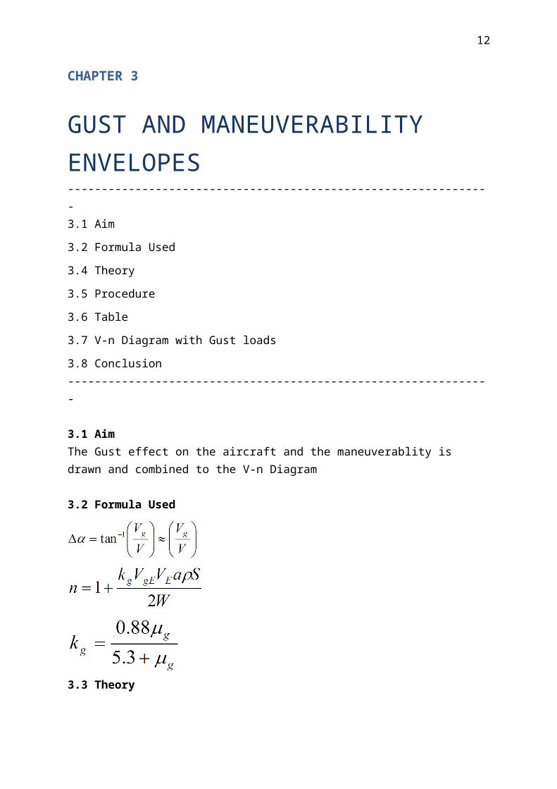
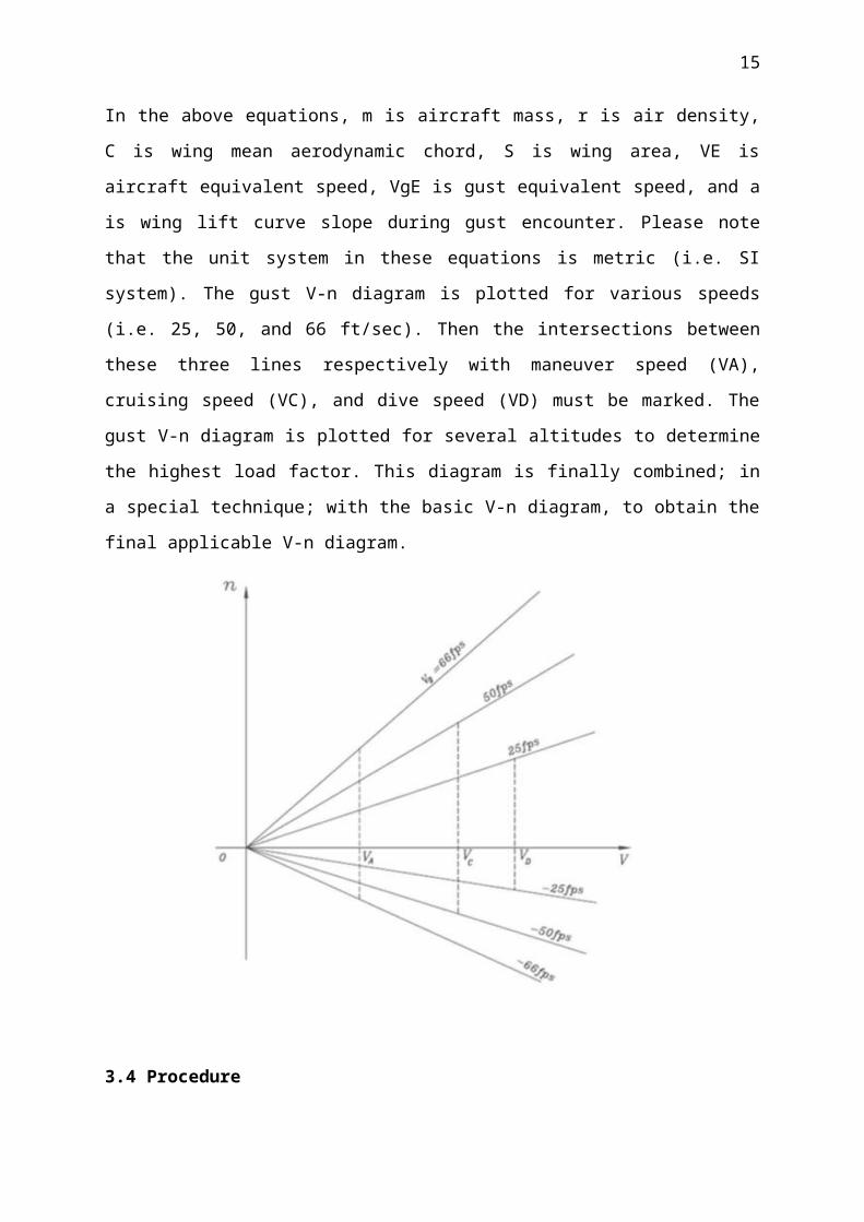
4.6 Graphs:

Span-wise Distribution:

20

Total Moment & Shear Load Distribution:

4.7 Conclusions

Thus the estimation of the load distribution along the span of the wing is found and graph is plotted.

21

CHAPTER 5

Load Distribution on Fuselage---------------------------------------------------------------5.1 Aim5.2 Formula Used5.3 Theory5.4 Procedure5.5 Tables5.6 Graphs5.7 Conclusion---------------------------------------------------------------

5.1 Aim To estimate the load distribution along the length of the fuselage and to draw the shear force and bending moment diagram

5.2 Formula Used

22

5.3 Theory The fuselage can be considered to be supported at the center of lift of the main wing.

The loads on the fuselage structure are then due to the shear force and bending moment about

that point. The loads come from a variety of components for example the weights of payload,

fuel, wing structure, tail structure, engines, fuselage structure, and tail control lift force. A

typical load distribution is shown below. The main aim of the fuselage of HALE aircraft is to

contain all mission equipment. In the preliminary assumption of configuration of HALE air-

craft the canard was built in the front of the fuselage. It was the reason why fuselage of PW-

111 was longed.

23

5.4 Procedure The fuselage structure can be considered to be a beam which is simply supported

and balancing at xCL The elemental forces and bending moments follow the formulas given,

with the exception that Δy in the case of the wing is replaced by Δx for the fuselage. The

equations are given as

24

The summation starts at one end of the fuselage (x=0 or x=L). In contrast the wing, the shear

force in the first element is considered to be load on that element, and the moment is con-

sidered to be the shear on that element. Starting at the selected end, the summation then con-

tinues across each element to the other end.

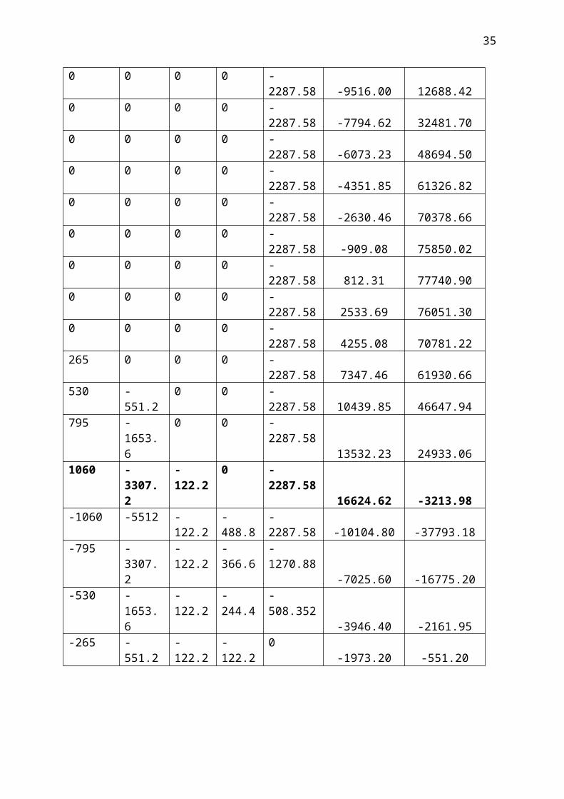
5.5 Table

Load Summary (Fuselage):

Load Summary Magnitude x/L-Start x/L - END Resultant dw

Fuel 7742 0.6 0.9 0.75 1106Payload 1760 0.2 0.8 0.5 135.38Structure 3172 0 1 0.5 1586Engine(s) 1266 0.8 0.8 0.8 1266Wing structure 2385 0.6 1 0.8 265Tail structure 611 0.8 1 0.9 122.2

Load Distribution along X (Fuselage):

X[ft] X/[b/2]

W-fuel V-fuel M-fuel W-Payload V-Payload M-Payload

0.00 0.00 0.00 0.00 16103.36 0.00 0.00 21964.802.08 0.05 0.00 0.00 16103.36 0.00 0.00 21964.804.16 0.10 0.00 0.00 16103.36 0.00 0.00 21964.806.24 0.15 0.00 0.00 16103.36 0.00 0.00 21964.808.32 0.20 0.00 0.00 16103.36 -135.38 0.00 21964.8010.40 0.25 0.00 0.00 16103.36 -135.38 135.38 21964.8012.48 0.30 0.00 0.00 16103.36 -135.38 270.77 21683.2014.56 0.35 0.00 0.00 16103.36 -135.38 406.15 21120.0016.64 0.40 0.00 0.00 16103.36 -135.38 541.54 20275.20

25

18.72 0.45 0.00 0.00 16103.36 -135.38 676.92 19148.8020.80 0.50 0.00 0.00 16103.36 -135.38 812.31 17740.8022.88 0.55 0.00 0.00 16103.36 -135.38 947.69 16051.2024.96 0.60 -1106.00 0.00 16103.36 -135.38 1083.08 14080.0027.04 0.65 -1106.00 1106.00 16103.36 -135.38 1218.46 11827.2029.12 0.70 -1106.00 2212.00 13802.88 -135.38 1353.85 9292.8031.20 0.75 -1106.00 3318.00 9201.92 -135.38 1489.23 6476.8033.28 0.80 -1106.00 4424.00 2300.48 -135.38 1624.62 3379.2035.36 0.85 -1106.00 -2212.00 -6901.44 0.00 0.00 0.0037.44 0.90 -1106.00 -1106.00 -2300.48 0.00 0.00 0.0039.52 0.95 0.00 0.00 0.00 0.00 0.00 0.0041.60 1.00 0.00 0.00 0.00 0.00 0.00 0.00

W-structure

V-structure

M-structure

W-Engine V-Engine M-Engine

W-Wing

-1586 -15860 -135254.08 0 0 0 0-1586 -14274 -102265.28 0 0 0 0-1586 -12688 -72575.36 0 0 0 0-1586 -11102 -46184.32 0 0 0 0-1586 -9516 -23092.16 0 0 0 0-1586 -7930 -3298.88 0 0 0 0-1586 -6344 13195.52 0 0 0 0-1586 -4758 26391.04 0 0 0 0-1586 -3172 36287.68 0 0 0 0-1586 -1586 42885.44 0 0 0 0-1586 0 46184.32 0 0 0 0W-structure

V-structure

M-structure

W-Engine V-Engine M-Engine

W-Wing

-1586 3172 42885.44 0 0 0 -265-1586 4758 36287.68 0 0 0 -265-1586 6344 26391.04 0 0 0 -265-1586 7930 13195.52 0 0 0 -265-1586 9516 -3298.88 -1266 0 0 -265-1586 -6344 -23092.16 0 0 0 -265-1586 -4758 -9896.64 0 0 0 -265-1586 -3172 0 0 0 0 -265-1586 -1586 0 0 0 0 -265

V-Wing M-Wing

W-Tail V-Tail M-Tail TOTAL V TOTAL M

0 0 0 0 -2287.58 -15860.00 -99473.50

26

0 0 0 0 -2287.58 -14274.00 -66484.700 0 0 0 -2287.58 -12688.00 -36794.780 0 0 0 -2287.58 -11102.00 -10403.740 0 0 0 -2287.58 -9516.00 12688.420 0 0 0 -2287.58 -7794.62 32481.700 0 0 0 -2287.58 -6073.23 48694.500 0 0 0 -2287.58 -4351.85 61326.820 0 0 0 -2287.58 -2630.46 70378.660 0 0 0 -2287.58 -909.08 75850.020 0 0 0 -2287.58 812.31 77740.900 0 0 0 -2287.58 2533.69 76051.300 0 0 0 -2287.58 4255.08 70781.22265 0 0 0 -2287.58 7347.46 61930.66530 -551.2 0 0 -2287.58 10439.85 46647.94795 -1653.6 0 0 -2287.58 13532.23 24933.061060 -3307.2 -122.2 0 -2287.58 16624.62 -3213.98-1060 -5512 -122.2 -488.8 -2287.58 -10104.80 -37793.18-795 -3307.2 -122.2 -366.6 -1270.88 -7025.60 -16775.20-530 -1653.6 -122.2 -244.4 -508.352 -3946.40 -2161.95-265 -551.2 -122.2 -122.2 0 -1973.20 -551.20

27

5.6 Graphs

Total Moment & Shear Load Distribution:

5.7 Conclusion Thus the estimation of the load distribution along the length of the fuselage and the graph between shear force and bending moment is plotted.

28

CHAPTER 6

Balancing and maneuvering loads on tail plane, Aileron and Rudder loads ---------------------------------------------------------------

6.1 Aim

6.2 Formula Used

6.3 Procedure

6.4 Model Calculation

6.5 Table

6.6 Drawing

6.7 Conclusion

---------------------------------------------------------------

6.1 Aim

To estimate the balancing and maneuvering loads on tail plane, aileron and rudder.

6.2 Formula Used

6.3 Theory:

Tail surfaces are used to both stabilize the aircraft and provide control moments

needed for maneuver and trim. Because these surfaces add wetted area and structural weight

they are often sized to be as small as possible. Although in some cases this is not optimal, the

tail is general sized based on the required control power as described in other sections of this

29

chapter. However, before this analysis can be undertaken, several configuration decisions are

needed. A large variety of tail shapes have been employed on aircraft over the past century.

These include configurations often denoted by the letters whose shapes they resemble in front

view: T, V, H, +, Y, inverted V. The selection of the particular configuration involves com-

plex system-level considerations, but here are a few of the reasons these geometries have

been used.

The conventional configuration with a low horizontal tail is a natural choice since roots of

both horizontal and vertical surfaces are conveniently attached directly to the fuselage. In this

design, the effectiveness of the vertical tail is large because interference with the fuselage and

horizontal tail increase its effective aspect ratio. Large areas of the tails are affected by the

converging fuselage flow, however, which can reduce the local dynamic pressure.

A T-tail is often chosen to move the horizontal tail away from engine exhaust and to reduce

aerodynamic interference. The vertical tail is quite effective, being 'end-plated' on one side by

the fuselage and on the other by the horizontal tail. By mounting the horizontal tail at the end

of a swept vertical, the tail length of the horizontal can be increased. This is especially

important for short-coupled designs such as business jets. The disadvantages of this

arrangement include higher vertical fin loads, potential flutter difficulties, and problems

associated with deep-stall.

One can mount the horizontal tail part-way up the vertical surface to obtain a cruciform tail.

In this arrangement the vertical tail does not benefit from the endplating effects obtained

either with conventional or T-tails, however, the structural issues with T-tails are mostly

avoided and the configuration may be necessary to avoid certain undesirable interference

effects, particularly near stall.

V-tails combine functions of horizontal and vertical tails. They are sometimes chosen

because of their increased ground clearance, reduced number of surface intersections, or

novel look, but require mixing of rudder and elevator controls and often exhibit reduced

control authority in combined yaw and pitch maneuvers.

H-tails use the vertical surfaces as endplates for the horizontal tail, increasing its effective

aspect ratio. The vertical surfaces can be made less tall since they enjoy some of the induced

drag savings associated with biplanes. H-tails are sometimes used on propeller aircraft to

reduce the yawing moment associated with propeller slipstream impingment on the vertical

tail. More complex control linkages and reduced ground clearance discourage their more

30

widespread use.

Y-shaped tails have been used on aircraft such as the LearFan, when the downward

projecting vertical surface can serve to protect a pusher propeller from ground strikes or can

reduce the 1-per-rev interference that would be more severe with a conventional arrangement

and a 2 or 4-bladed prop. Inverted V-tails have some of the same features and problems with

ground clearance, while producing a favorable rolling moments with yaw control input

The correlation is based on a fuselage destabilizing parameter:

hf is the fuselage height

wf is the fuselage width

Lf is the fuselage length

Sw, cw, and b are the wing area, MAC, and span and provides a rough estimate for the

required horizontal tail volume (Vh = lh Sh / cw Sw) and vertical tail volume (Vv = lv Sv / b

Sw). Recall that lh and lv are the distances from the c.g. to the a.c. of the horizontal and

vertical tails

Where

VV is the vertical tail volume coefficient

31

SV is the area of the rudder

lV is the distance from the centre of gravity to the quarter chord of the rudder

S is the wing area

b is the wing span

A value suggested for the vertical tail coefficient VV is 0.035

The primary function of an aileron is the lateral (i.e. roll) control of an aircraft; however, it

also affects the directional control. Due to this reason, the aileron and the rudder are usually

designed concurrently. Lateral control is governed primarily through a roll rate (P). Aileron is

32

structurally part of the wing, and has two pieces; each located on the trailing edge of the

outer portion of the wing left and right sections. Both ailerons are often used symmetrically,

hence their geometries are identical. Aileron effectiveness is a measure of how good the

deflected aileron is producing the desired rolling moment. The generated rolling moment is

a function of aileron size, aileron deflection, and its distance from the aircraft fuselage

centre line. Unlike rudder and elevator which are displacement control, the aileron is a rate

control. Any change in the aileron geometry or deflection will change the roll rate; which

subsequently varies constantly the roll angle.

The deflection of any control surface including the aileron involves a hinge moment. The

hinge moments are the aerodynamic moments that must be overcome to deflect the con-

trol surfaces. The hinge moment governs the magnitude of augmented pilot force required

to move the corresponding actuator to deflect the control surface. To minimize the size and

thus the cost of the actuation system, the ailerons should be designed so that the control

forces are as low as possible.

33

In the design process of an aileron, four parameters need to be determined. They are: 1. ail -

eron planform area (Sa); 2. aileron chord/span (Ca/ba); 3. maximum up and down aileron de-

flection ( Amax); and 4. location of inner edge of the aileron along the wing span (bai).

Figure 12.10 shows the aileron geometry. As a general guidance, the typical values for these

parameters are as follows: Sa/S = 0.05 to 0.1, ba/b = 0.2-0.3, Ca/C = 0.15-0.25, bai/b = 0.6-

0.8, and Amax = 30 degrees. Based on this statistics, about 5 to 10 percent of the wing area

is devoted to the aileron, the aileron-to-wing-chord ratio is about 15 to 25 percent, aileron-to-

wing-span ratio is about 20-30 percent, and the inboard aileron span is about 60 to 80 percent

of the wing span.

34

6.7 Conclusion: Thus the estimation of the balancing and maneuvering loads on tail plane, aileron and

rudder is completed.

35

Chapter 7

Structural Layout The main changes to the initial aircraft layout, from the work done

so far, are associated with the provision for adequate lateral (weathercock) stability and

control. The long-span, forward-swept wing with winglets, and the long forward fuselage

with deep side area, will generate destabilising moments in cross-wind conditions. Balancing

these moments is difficult due to the relatively short tail arm. Two modifications are

proposed to ease this problem. The forward fuselage length is to be reduced by 2 metres

and ‘finlets’ are to be placed on the wing outboard of the inner wing trailing edge control

surfaces. These finlets could be made large enough to double the original fin area if

required. Some of the loss of equipment volume resulting from the reduction of the

fuselage length could be regained by moving the fuselage fuel tank further back and

increasing the amount of fuel held in the wing. These two proposals together should provide

sufficient flexibility into the layout to overcome the perceived stability problem. A second

concern relates to the layout of the landing gear. The large wing-span, high aircraft centre of

gravity and the narrow main-wheel track combine to make the aircraft potentially unstable

in taxi, take-off and landing conditions. The reduced length of the forward fuselage

mentioned above will improve the landing gear geometry but this will not be sufficient. It

will be necessary to increase the track of the main wheels. This can only be done by adding

fuselage sponsons at the main undercarriage mounting positions. Increasing the track to 4

m will provide an overturning angle of about 52◦ (convention suggests that an angle greater

than 60◦ is unsafe or twitchy in operation). The sponsons will need to be extended fore and

aft to provide aerodynamic blending. These extensions will provide extra storage. This new

arrangement will also improve the attachment geometry of the braces at the side of the

fuselage. Following the calculations of the component masses and the associated aircraft

centre of gravity assessment the wing leading edge sweep will be reduced from 30 to 25◦.

The above changes have been included into a revised aircraft general arrangement drawing,

36

37

Chapter 8

ConclusionThere are many further design considerations to be studied in the development of this project.

The aircraft is a complex combination of advanced technologies in aerodynamics, structures,

materials, stability and system integration. This represents a substantial challenge which re-

flects the nature of future aircraft project work. As aero-nautical design matures it will be-

come harder to make significant improvements to current designs. This will force aeronaut-

ical engineers to introduce innovation into new designs. The ability to handle the necessary

analysis methods to reduce technical risk will form a major feature of future design teams.

These teams will include many more specialists from disciplines that have not been tradition-

ally included in aircraft project design. Organising, managing and controlling these teams

will demand skills other than those conventionally related to aeronautical engineering. A

more ‘system-orientated’ approach will become the new practice.

As well as dealing with the integration of new technologies and methods, this project has in-

volved the analysis of aircraft operating in the higher atmosphere. In this environment, the

stall and buffet flight boundaries begin to converge to make control more difficult. High-

speed, high-alpha must be carefully considered to ensure that the aircraft is dynamically

stable yet, as in this case, aerodynamically efficient. This combination offers a serious test to

the aerodynamic and structural disciplines. This project has demonstrated the unique features

of designing an aircraft to account for:

· uninhabited/autonomous missions,

· fast and high operation,

· system and airframe integration,

Not many new projects incorporate such a mixture of challenges to the design team. How-

ever, if the difficulties of meeting such demands can be successfully achieved without jeop-

ardising aircraft operational integrity, then we will be in the enviable position of ‘pushing the

envelope’.

38

Chapter 9

References1) Aircraft Design by Thomas . C. Corke, University of Notre Dame.2) Aircraft Design – A Conceptual Approach by Raymer.3) Kampf, K. P., ‘Design of an unmanned reconnaissance system’, ICAS 2000, Harrogate

UK, August 2000.4) AIAA Aerospace Design Engineers Guide, AIAA Publications, ISBN 0-939403-21-5,

1987. 5) Brassey’s World Aircraft & Systems Directory, Brassey Publications, ISBN 1-57488-

063-2. 6) Jane’s All the World’s Aircraft, Jane’s Annual Publication, various years. See

www.janes.com for list of publications. 7) Lange, R. H., ‘Review of unconventional aircraft design concepts’, Journal of Aircraft

25, 5: 385–392. 8) Ko, A. et al. ‘Effects of constraints in multi-disciplinary design of a commercial

transport with strut-braced wings’. AIAA/SAE World Aviation Congress 2000/1, paper 5609.

9) Gundlach, J. T. et al. ‘Concept design studies of a strut-braced wing, transonic transport’.

10) AIAA Journal of Aircraft, Vol. 137, No. 6, Nov-Dec 2000, pp. 976–983. 11) Jenkinson, L. R. et al., Civil Jet Aircraft Design, Butterworth-Heinemann, 2000, ISBN 0-

340741-52-X.