1 AJF Deployment Scenarios – ASCENT/ FTOT/ BSM Collaboration FAA Project Manager:Nathan Brown The National Transportation Systems Center Advancing transportation innovation for the public good U.S. Department of Transportation Office of the Secretary of Transportation John A. Volpe National Transportation Systems Center
Transcript
1
AJF Deployment Scenarios –
ASCENT/ FTOT/ BSM Collaboration
FAA Project Manager: Nathan Brown
The National Transportation Systems Center
Advancing transportation innovation for the public good
U.S. Department of Transportation
Office of the Secretary of Transportation
John A. Volpe National Transportation Systems Center
2
Objective
Analysis focused on two questions:
1) How much AJF can be produced and how soon?
2) What is the likely geospatial distribution of feedstock and fuel production and AJF delivery?
3
Scenario Elements
Included ASTM-approved pathways: HEFA, FT, and ATJ
Experience with AJF production has shown that there is a significant lag prior to commercialization after approval
TEA data and product slates from A01 Research
Feedstocks evaluated (projected to 2030 for FTOT analysis)
Waste fats, oils and greases – HEFA
Municipal solid waste (MSW) – FT
Woody residues – FT or ATJ
Agricultural residues – ATJ
4
Modeling Approach
ASCENT Research Product slates/efficiency
Technoeconomics
Feedstock availability scenarios
National Renewable Energy Laboratory (NREL) Biomass Scenario Model (BSM) System dynamics modeling of influence of incentives on deployment
trajectories from 2017-2045
Volpe Center Freight and Fuel Transportation Optimization Tool (FTOT) Optimal geospatial patterns of transport and delivery in 2030
5
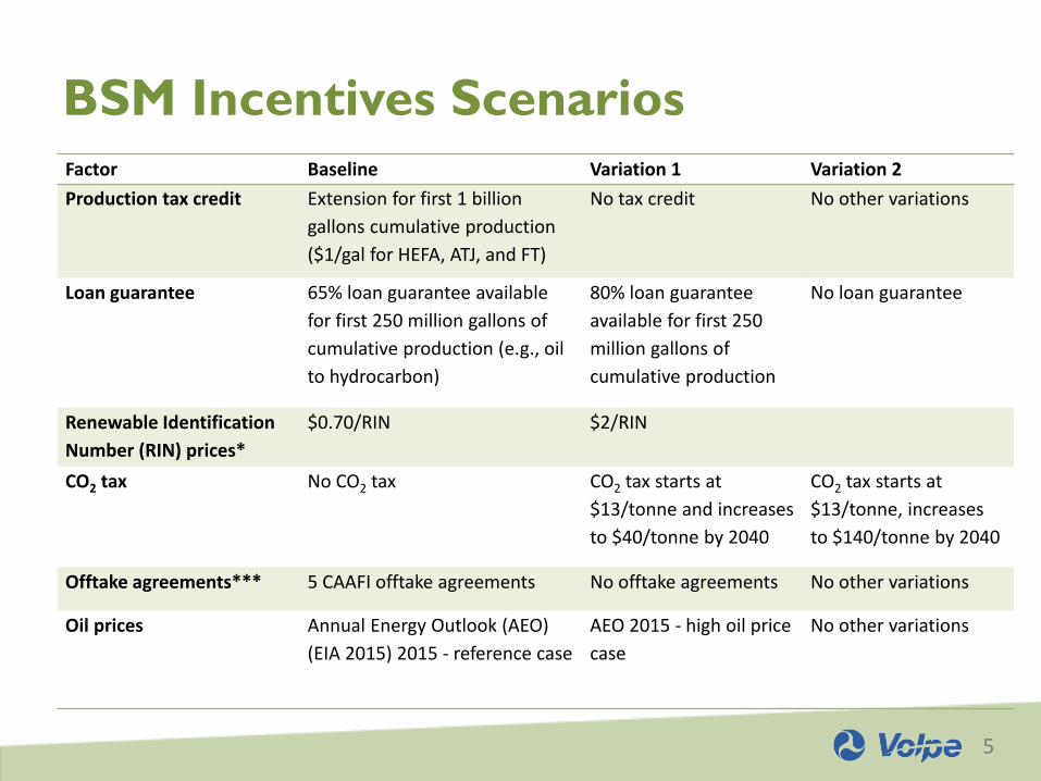
BSM Incentives Scenarios
Factor Baseline Variation 1 Variation 2
Production tax credit Extension for first 1 billion
gallons cumulative production
($1/gal for HEFA, ATJ, and FT)
No tax credit No other variations
Loan guarantee 65% loan guarantee available
for first 250 million gallons of
cumulative production (e.g., oil
to hydrocarbon)
80% loan guarantee
available for first 250
million gallons of
cumulative production
No loan guarantee
Renewable Identification
Number (RIN) prices*
$0.70/RIN $2/RIN
CO2 tax No CO2 tax CO2 tax starts at
$13/tonne and increases
to $40/tonne by 2040
CO2 tax starts at
$13/tonne, increases
to $140/tonne by 2040
Offtake agreements*** 5 CAAFI offtake agreements No offtake agreements No other variations
Oil prices Annual Energy Outlook (AEO)
(EIA 2015) 2015 - reference case
AEO 2015 - high oil price
case
No other variations
6
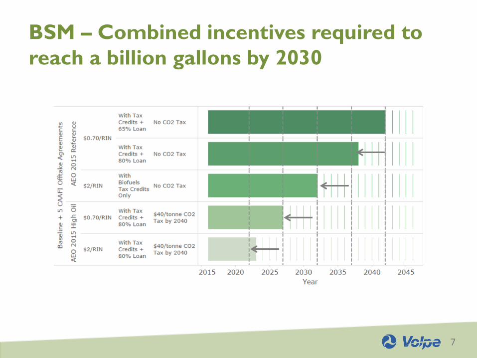
38% of scenarios result in more than
one billion gallons in 2030
7
BSM – Combined incentives required to
reach a billion gallons by 2030
8
ASCENT Feedstock Projections
Feedstock
Available in
2030
Data Source Data Details
Scenario-specific
proportion of
feedstock available for
conversion
Low High
Waste FOG Adapted from inedible
waste animal fat
rendering data
Animal inventory per acre of
farmland, county level. Only
includes inedible FOG.
30% 50%
MSW Adapted from EPA (2013)
and World Bank (2025)
per capita values adjusted
to 2030
Per capita applied to
population, county level.
Excludes already recycled,
composted, or not convertible
30% 50%
Forest
residues
Land Use and Resource
Allocation (LURA)
modeling
FIA points, aggregated to
county level; Average of 20
years based on market.
30% 50%
Crop
residues
POLYSYS modeling by
University of Tennessee
County level Avail. @
$50/dry ton
$60/dry
ton
9
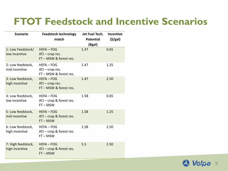
FTOT Feedstock and Incentive ScenariosScenario Feedstock technology
match
Jet Fuel Tech.
Potential
(Bgal)
Incentive
($/gal)
1: Low Feedstock/ low incentive
HEFA – FOGATJ – crop res.FT – MSW & forest res.
1.47 0.65
2: Low feedstock, mid incentive
HEFA – FOGATJ – crop res.FT – MSW & forest res.
1.47 1.25
3: Low feedstock, high incentive
HEFA – FOGATJ – crop res.FT – MSW & forest res.
1.47 2.50
4: Low feedstock, low incentive
HEFA – FOGATJ – crop & forest res.FT – MSW
1.58 0.65
5: Low feedstock, mid incentive
HEFA – FOGATJ – crop & forest res.FT – MSW
1.58 1.25
6: Low feedstock, high incentive
HEFA – FOGATJ – crop & forest res.FT – MSW
1.58 2.50
7: High feedstock, high incentive
HEFA – FOGATJ – crop & forest res.FT – MSW
5.5 2.50
10
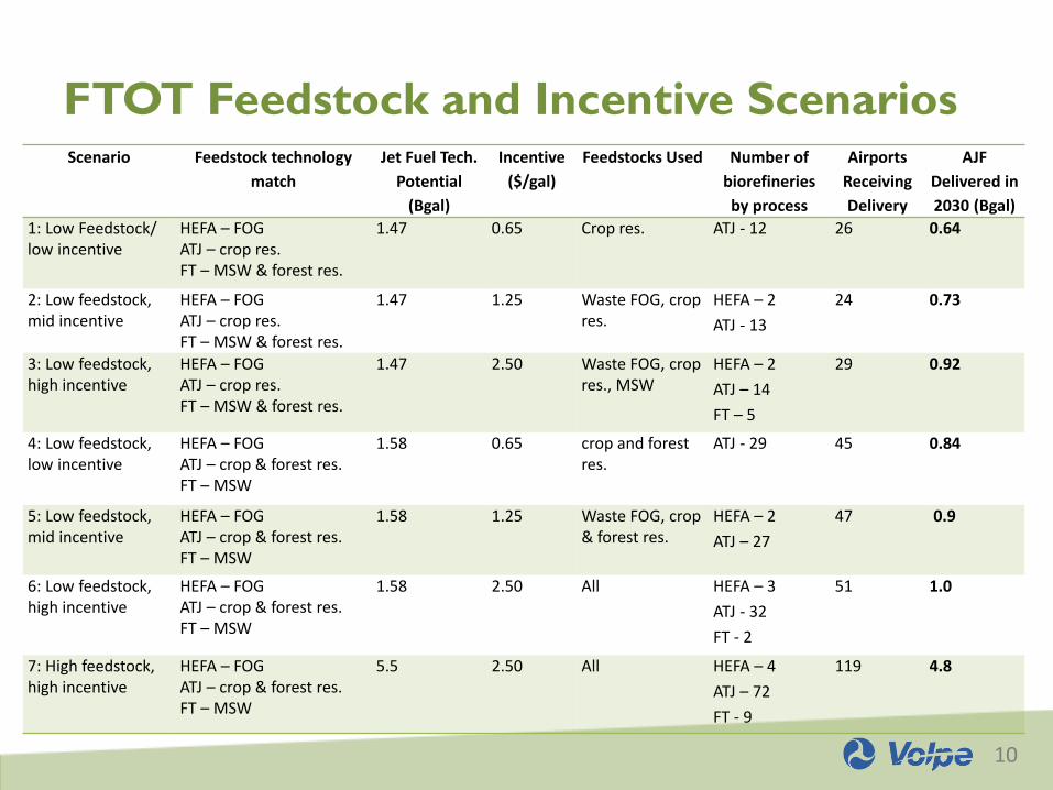
FTOT Feedstock and Incentive ScenariosScenario Feedstock technology
match
Jet Fuel Tech.
Potential
(Bgal)
Incentive
($/gal)
Feedstocks Used Number of
biorefineries
by process
Airports
Receiving
Delivery
AJF
Delivered in
2030 (Bgal)
1: Low Feedstock/ low incentive
HEFA – FOGATJ – crop res.FT – MSW & forest res.
1.47 0.65 Crop res. ATJ - 12 26 0.64
2: Low feedstock, mid incentive
HEFA – FOGATJ – crop res.FT – MSW & forest res.
1.47 1.25 Waste FOG, crop res.
HEFA – 2
ATJ - 13
24 0.73
3: Low feedstock, high incentive
HEFA – FOGATJ – crop res.FT – MSW & forest res.
1.47 2.50 Waste FOG, crop res., MSW
HEFA – 2
ATJ – 14
FT – 5
29 0.92
4: Low feedstock, low incentive
HEFA – FOGATJ – crop & forest res.FT – MSW
1.58 0.65 crop and forest res.
ATJ - 29 45 0.84
5: Low feedstock, mid incentive
HEFA – FOGATJ – crop & forest res.FT – MSW
1.58 1.25 Waste FOG, crop & forest res.
HEFA – 2
ATJ – 27
47 0.9
6: Low feedstock, high incentive
HEFA – FOGATJ – crop & forest res.FT – MSW
1.58 2.50 All HEFA – 3
ATJ - 32
FT - 2
51 1.0
7: High feedstock, high incentive
HEFA – FOGATJ – crop & forest res.FT – MSW
5.5 2.50 All HEFA – 4
ATJ – 72
FT - 9
119 4.8
11
BSM and FTOT Results Comparison
FTOT results for low feedstock availability are well within BSM results
High feedstock availability scenario exceeds BSM results
•
••
•
•
••
FTOT Results
• Technical Potential
• AJF Delivered
12
FTOT Geographic Results
ATJ – crop residues only, FT –MSW, forest residues
Low incentive ATJ only
Mid incentive ATJ, HEFA
High incentive ATJ, HEFA, FT
Increasing incentive expanded feedstock draw
Primary mode - rail. Pipeline largely unavailable near ATJ
Average Transport Cost = $0.69-0.84/gal
13
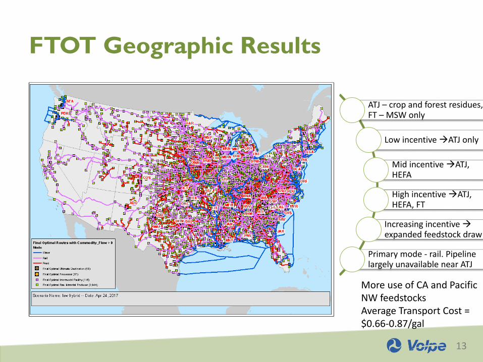
FTOT Geographic Results
ATJ – crop and forest residues, FT – MSW only
Low incentive ATJ only
Mid incentive ATJ, HEFA
High incentive ATJ, HEFA, FT
Increasing incentive expanded feedstock draw
Primary mode - rail. Pipeline largely unavailable near ATJ
More use of CA and Pacific NW feedstocksAverage Transport Cost = $0.66-0.87/gal
14
Conclusions
A billion gallons per year of AJF production in 2030 is possible
Will require a combination of incentives to achieve a billion gallons or more
Waste feedstocks (crop residues) are likely to be drawn from Midwest first if existing ethanol facilities can be repurposed to ATJ
Pipeline infrastructure may not be ready for drop-in fuels production in Midwest
Models can inform each other to improve future analyses
FTOT uses nth plant/fixed efficiency – BSM could output an estimated efficiency for a particular year based on scenarios and maturation curve