50
ALASKA ECONOMIC FORECAST FOR 1977 Daniel A. Seiver Institute of Social and Economic Research University of Alaska 707 "A" Street, Suite 206 Anchorage, Alaska 99501 March 2, 1977

ALASKA ECONOMIC FORECAST FOR 1977
Daniel A. Seiver Institute of Social and Economic Research
University of Alaska 707 "A" Street, Suite 206 Anchorage, Alaska 99501
March 2, 1977

-

ALASKA ECONOMIC FORECAST FOR 1977
1, Summary and Highlights
Alaska economic activity will experience a significant decline
in 1977 as the trans-Alaska oil pipeline is completed, The unem
ployment rate will be substantially higher than in recent years,
the rate of inflation (as measured by the Anchorage Consumer Price
Index) will be the lowest since 1973. Almost all of Alaska's support
sectors will be adversely affected, with substantial employment de
clines in services and trade, two of the largest groups of employers
in the state. Overall employment in the state will fall by 14 per
cent below 1976. This decline will occur in spite of assumed rapid
increases in employment in the mining, manufacturing, and agriculture,
forestry, and fisheries sectors. Detailed forecasts:
UNEMPLOYMENT RATE: 12.1% for 1977 (highest ever recorded) 13.4% for first quarter of 1977 (highest in 3 years)
PRICES: 6.3% higher in 1977 (Anchorage C.P.I.) 5.6% for fourth quarter of 1977
CIVILIAN EMPLOYMENT: Down 14% compared to 1976 last quarter of 1977 lowest since mid-1974

EMPLOYMENT BY SECTOR:
Trade: Down 13.6% compared to 1976
Services: Down 17.9% compared to 1976
Construction: Down 46.4% compared to 1976
Transportation, Communication, and Public Utilities Down 17.4% compared to 1976
Finance, Insurance, and Real Estate: Down 18.3% compared to 1976
State and Local Government: Up 2.6% compared to 1976
2. Assumptions Made for the Forecast*
United States
U.S. Consumer Prices:
U.S. Wages:
Up 7% over 1976
Up 8% over 1976
Alaska
Mining Employment:
~':·h Manufacturing Employment:
Agriculture, Forestry, Fisheries Employment:
Federal Government Employment:
Up 15% over 1976
Up 15% over 1976
Up 15% over 1976
Unchanged in 1977
2
Pipeline Employment: 5,000 in 1977 (by quarter: 7,500; 8,000; 4,000; 2,000)
Note: These assumptions are not derived from I.S.E.R. 's econometric model, Rather, they are necessary inputs to the model (See Section 4). The accuracy of the forecast may depend in part on the accuracy of these assumptions.
*section 4 of this report explains the role of these assumptions in making forecasts of economic activity,
**Food, lumber, and paper

3
3, Forecast Discussion
Figures 1-9 on the following pages depict the extent of the
decline forecast for 1977. Preliminary employment data for the
first two quarters of 1976 are also shown on the forecast graphs,
which can be compared with the 1976 results generated by the econo
metric model. 1'
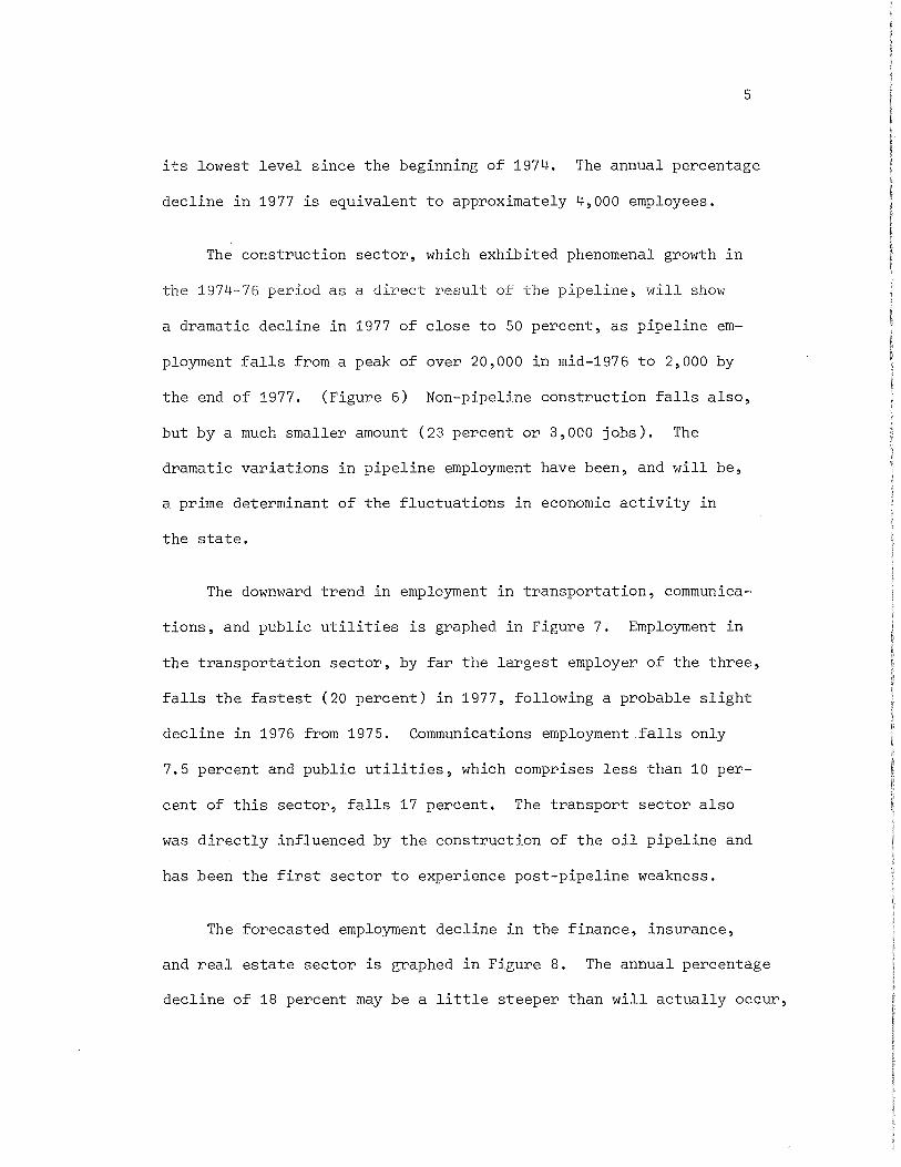
Figure 1 shows a rapid increase for the state's unemployment
rate beginning in the fourth quarter of 1976. (Very preliminary
data for the last half of 1976 suggests this rise has in fact taken
place.) The peak of 13.4 percent in the first quarter of 1977 is
higher than any quarter in the last three years, but still not as
high as the rate for 1974:1, In 1977, however, unlike previous
years, the unemployment rate will not fall dramatically in the
second and third quarters, and again exceeds 13 percent in the
fourth quarter, Thus, the annual average of 12.1 percent will be
the highest since record-keeping began in 1947.
Figure 2 presents our forecast for civilian wage and salary
employment. The mid-year surge of 1975 and 1976, as the pipeline
workforce rose to its peak, will be sharply attenuated in 1977,
By the fourth quarter of 1977, with the pipeline construction work
force down to 2,000, employment will fall to the lowest level since
*The creation and testing of the model is discussed in Section 4.

1974:2, the commencement of the pipeline boom, The 1977 average
shows a 14 percent decline from 1976, the sharpest decline since
record-keeping began in 1947.
Price inflation will continue the moderating trend of 1976,
with prices rising only 6.3 percent for the year, and increasing
4
at an annual rate of only 5.6 percent by the end of 1977. This
trend is graphed in Figure 3. The rate of inflation in Alaska is
measured by the change in the Anchorage Consumer Price Index.
Prices in other areas of the state, notably Fairbanks, may increase
even more slowly. The 1977 rate of inflation is, however, still
rather rapid compared to the pre-1974 years of mild inflation,
The trade sector is one of the largest support sectors in the
Alaska economy, and employment falls by 13,6 percent in 1977, or
approximately 3,500 employees. This decline (graphed in Figure 4)
accounts for a sizable portion of the overall decline in employment.
A major portion of this decline will occur in Anchorage, which ac
counts for three-quarters of the trade employment in the state,
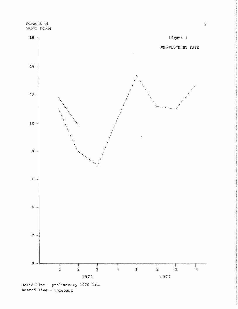
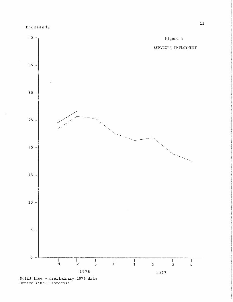
A slightly more severe decline occurs in the service sector
of the state economy, graphed in Figure 5, The annual percentage
decline of about 18 percent again will be concentrated in Anchorage,
the service center of the state. The fourth quarter of the year
will be the low point for 1977, with service employment falling to
5
its lowest level since the beginning of 1974. The annual percentage
decline in 1977 is equivalent to approximately 4,000 employees.
The construction sector, which exhibited phenomenal growth in
the 1974-76 period as a direct result of the pipeline, will show
a dramatic decline in 1977 of close to 50 percent, as pipeline em
ployment falls from a peak of over 20,000 in mid-1976 to 2,000 by
the end of 1977. (Figure 6) Non-pipeline construction falls also,
but by a much smaller amount (23 percent or 3,000 jobs). The
dramatic variations in pipeline employment have been, and will be,
a prime determinant of the fluctuations in economic activity in
the state.
The downward trend in employment in transportation, communica
tions, and public utilities is graphed in Figure 7. Employment in
the transportation sector, by far the largest employer of the three,
falls the fastest (20 percent) in 1977, following a probable slight
decline in 1976 from 1975. Communications employment.falls only
7.5 percent and public utilities, which comprises less than 10 per
cent of this sector, falls 17 percent. The transport sector also
was directly influenced by the construction of the oil pipeline and
has been the first sector to experience post-pipeline weakness.
The forecasted employment decline in the finance, insurance,
and real estate sector is graphed in Figure 8. The annual percentage
decline of 18 percent may be a little steeper than will actually occur,

6
based on very preliminary data for the last two quarters of 1976.
Again, the major portion of this decline will take place in Anchor
age, which is the financial center of the state.
Last, but certainly not least of the support sectors of the
economy, is state and local government. Employment in this sector
is forecasted to rise in 1977, reflecting higher spending levels
by the state in fiscal year 1977 and especially fiscal year 1978,
beginning July 1, 1977. This increase in employment will have an
ameliorating effect on the decline in economic activity, but cannot
prevent it. Figure 9 shows the forecasted trend in state and local
government employment. Employment in this sector showed little
growth in 1976, in contrast to the rapid growth in most other
sectors.
The I.S.E.R. short-run model cannot make regional forecasts.
Yet it is obvious that much of the forecasted decline in employment
will take place in the Anchorage area, which accounts for more than
half of the state's support sector employment, The Fairbanks area
will no doubt suffer a greater relative decline in employment, and
probably higher unemployment also, given the dramatic boom in the
area in 1974-1976.
Percent of Labor Force
16 -
14 -
12 -
10 -
8 -
6 -
4 -
2 -
\ \
\
\ \
\ \ \
\
"-' I ''- I
'I
I I
I
I I
I
I I
Figure 1
UNEMPLOYMENT RATE
/\ I \
I \ I \
I ' / \
I '"-- / I ----J
/
/
/ /
/
7
o-~-------~-----------~---~----·-----~---1 2 3
1976
Solid line - preliminary 1976 data
Dotted line - forecast
4 1 2 3 4
1977

8 thousands
200 - Figure 2
CIVILIAN WAGE AND SALARY EMPLOYMENT
175 -
\ \
\
"' 150 -/
/
125 -
100 -
75 -
50 -
25 -
o-~--~---~,----,----,----,----,---------1 2 3 4 1 2
1976
Solid line - preliminary 1976 data Dotted line - forecast
3 4
1977

annual percent increase
16 -
14 -
12 -
1 2
1976
(actual)
3 4 1
Figure 3
INFLATION RATE (Anchorage CPI)
2 3
1977
(forecast)
4
9

10 thousands
40 - Figure 4
TRADE EMPLOYMENT
35 -
30 -
25 -
"
20 -
15 -
10 -
5 -
0 -'---------·----,-"---;----·+-----"f-----;---------
1 2 3
1976
Solid line - preliminary 1976 data Dotted line - forecast
1 2 3 4
1977
11 thousands
40 - Figure 5
SERVICES EMPLOYMENT
35 -
30 -
25 - - - -, /
20 -
15 -
10 -
5 -
0 - ·------------------------------------1 I I I I I 1 2 3 4 1 2 3 4
1976
Solid line - preliminary 1976 data Dotted line - forecast
1977

thousands
40 -
35 -
30 -
25 -
20 -
15 -
10
5 -
1/
1/
'/
I.
/
(
/\ / / \
\ \ \
\
\ \ \
\ \
\ \
\
\ \ \
Figure 6
CONSTRUCTION EMPLOYMENT
/ "\ \ / \
\ / \ v/ \
\ \
\ \
\ \
\ \
\
12
o-~---··Tr==-T,---,----,-----r-----,----~---,---1 2 3
1976
Solid line - preliminary 1976 forecast Dotted line - forecast
4 1 2 3 4
1977

thousands
20 -
15 -
1 2 3
1976
Solid line - preliminary 1976 data Dotted line - forecast
4- 1
13
Figure 7
TRANSPORTATION, COMMUNICATION, AND UTILITIES EMPLOYMENT
2 3 4-
1977

thousands
8 -·
7 -
6 -
5 -
4 -
3 -
2 -
1 -
14
Figure 8
FINANCE, INSURANCE, AND REAL ESTATE EMPLOYMENT
-'\ \.
- --
o-~---~---~---~---~---~~--~~---1 2 3
1976
Solid line - preliminary 1976 data Dotted line - foLecast
4 1 2 3 4
1977

thousands
40 -
35 -
30 - --
25 -
20 -
15 -
10 -
5 -
-
15
Figure 9
STATE AND LOCAL GOVERNMENT EMPLOYMENT
/
/ /
/
-/ --
o-~--~---~--~i----,----1----,----1----,--1 2 3 4 1 2 3 4
1976 Solid line - preliminary 1976 data Dotted line - forecast
1977
4. Description and Background of I.S.E.R. 's Quarterly Econometric Model*
Beginning in 1978, the state of Alaska will receive almost
one billion dollars per year in royalties and taxes from Prudhoe
Bay oil production, The long-term consequences of this massive
flow of "petrodollars" have been studied by the Institute of
Social and Economic Research at the University of Alaska for the
past three years. Several long-run policy-oriented econometric
models of the state have been constructed, These models are
driven by resource development scenarios which project the employ
ment and revenue impacts of further development of Alaska's petro
leum resources, and by state expenditures, a key policy variable
which, given the massive "petrodollar" flows, can be manipulated
by policymakers with major effects on the economy.**
Long-term models of Alaska's economy tend to show relatively
smooth and steady growth. Yet quite recent experience is demon
strating once again the "boom-bust" nature of the Alaska economy.
In order to capture the short-run characteristics of the Alaska
economy, a quarterly econometric model has been constructed and
*A more detailed and technical discussion of model construction, estimation, and testing is contained in Daniel A. Seiver, "A Quarterly Model of the Alaska Economy," February, 1977. This model was created using the TROLL system of the National Bureau of Economic Research, Inc.
16
~h':These models are described in detail in David T. Kresge, 11Alaska I s Growth to 1990, 11 Alaska Review of Business and Economic Conditions, vol. 13, no. 1, January, 1976.

has been tested against historical data, and used for the forecast
discussed above.
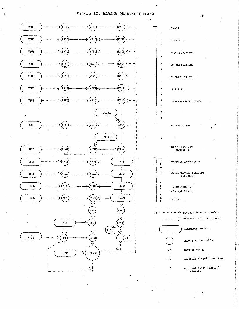
The structure of the model is diagrammed in Figure 10, The
symbolic notation can be decoded by referring to the symbol die-
tionary on page All "Q" suffixes have been deleted from
Figure 10 to simplify the diagram.
17
Employment in Alaska's support sectors is a function of local
demand, which is measured by real disposable personal income (DPIRQS),
Almost all the demand-employment relations contain seasonal dummies,
reflecting the highly seasonal nature of the Alaska economy. Those
variables which do not exhibit seasonal variation are marked with .,.
an asterisk," Several support sector employment equations have
slightly differing specifications. During the historical period,
much of the communications network was turned over to private in-
dustry by the Federal government, and a special dummy has been
added to the communications employment equation to account for this
transfer. The transport sector, particularly trucking and air trans
port, has been exogenously affected by oil development and pipeline
construction: a special dummy has been added to the transport em
ployment equation to capture this effect. During the pipeline con
struction boom, construction employment has a large exogenous com
ponent (ECONXQ) which is forecasted separately based on periodic
*Appendix A lists all the equations in the model and contains regression results for all stochastic equations.
... Figure 10. ALASKA QUAR'l'ERLY
c~-~u~_-_)-->6---------> 11:;~J'J ~------€~~~-<· - ·1 I
( __ ~~~-)- ->8------>ES'J <---
c_~J- 7'8- €p<-C \/£:US )~ ..;::, s-~wsc~½ ., X' c-WE0- ~ s------;r('PU
(!~us-)-
( WEUS )- ---->8
C WEUS )- -->
C
C 1/EUS )-
C WEUS )-
CiEUS~- - - - ~
(..__ __ m_ic_s __
Q~)---,, ,,
(
I ,_ .t,. I -· _J
.1
-1
·- I
<-
-, I
I
I.
MODEL
s
u p
p
0
R
T
s E
C
T
0
R-
s
"E, X p
0 R T"
s E C T 0 R s
18
TRAD£:
SERVICES
TRANSPORTATION
COMMUNICATIONS
PUBLIC UTILITIES
F,I.R,£:,
MANUFACTURING-OTHER
CONSTRUCTION
STATE AND LOCAL GOVERNMENT
IBDERAL GOVERIH-!£:N'f
AGRICULTURE, !'ORESTRY, FISHERIES
MANJ.)FACTURll!G
(Except Other')
MIIIIHG
KEY - - - - :;;> stochastic relationship
definitional relation,:;hip
C _)
0 b.
- k
,,
exogenou~ variable
endogcnouc variable
rate of change
variable Jagged k quart~r,,
no s!r,nJ f icunt scuuonal Vill'lation

19
SYMBOL DICTIONARY
Sector Symbol Sector Symbol
Ag,, For,, Fish, A9 Manufacturing (except other) MB Communications CM Mining pg Construction CN Public Utilities PU Federal Government GF Services Federal Military GM State and F.I.R.E, FI Trade Manufacturing (Other) MO Transport
OTHER VARIABLES
Symbol
DNCSQ
DPIQ DPIRQ
DPIRQS E99SFQ
ECONXQ
EM9CQ LFCQ
Name
Federal Payment for Alaska Native Claims Settlement Act
Disposable Personal Income Real Disposable Personal
Income DPIRQ Seasonally Adjusted State Government Non-Capital
Expenditures Exogenous Construction
Employment Civilian Employment Civilian Labor Force
Symbol
PC RPIQ S(i)
SFAC UQ URATE WEUSQ WS99Q
VARIABLE PREFIXES
Coefficient - C Employment - EM
Wage Rate - WR Wages and Salaries - WS
S9 Local Government SL
D9 T9
Name
U.S.C,P.I. Alaska Relative Price Index Seasonal Dummy for ith
Quarter (i-1,2,3) Seasonal Adjustment Factors Unemployment Unemployment Rate U.S. Average Weekly Earnings Total Wages and Salaries
Rate of Change - DEL(~)

employment and employment projection reports obtained from the
pipeline construction consortium. The endogenous component of
construction is estimated first, using the standard support sector
specification, and then exogenous construction employment is added
to determine total construction employment.
Wage rates (average earnings per quarter) in the support
sectors are functions of U.S. quarterly average weekly earnings
(WEUSQ). Most of the historical variation in support sector wage
rates can be explained with this variable and seasonal dummy vari
ables. However, the pipeline construction boom has had a major
impact on all wage rates in Alaska. To capture this effect, a
dummy variable, ECONXQ/EMCNQ, has been added to most wage rate
equations.
20
The "export" sectors of the model have exogenously determined
employment levels, but endogenously determined wage rates, Federal
government employment has changed relatively little over the his
torical period, Most of the manufacturing employment in Alaska
consists of food (fish) processing (45 percent of 1975 manufacturing
employment) and lumber and paper manufacturing (35 percent of 1975
manufacturing employment). Most lumber and paper output is exported
to Japan, and food processing employment depends crucially on the
sizes of the relevant harvests of fish. It is thus not feasible
to tie what manufacturing employment Alaska does have to the

national economy. The remainder of manufacturing employment is
responsive to local demand and is treated as a support sector.
21
Agriculture, forestry, and fisheries is a heterogenous sector
for which employment is also determined outside the model. Alaska
has almost no agriculture. Forestry employment is heavily depend
ent on supply management considerations, and fisheries employment
depends on supply considerations also. Total employment in agricul
ture, forestry, and fisheries comprises less than one percent of
total civilian employment.
Mining employment in Alaska is essentially petroleum employ
ment, which is not sensitive to either local or national aggregate
demand conditions. Independent projections of mining employment
are contained in the resource development scenarios of I.S.E.R. 's
long-run models.
The state and local government sector is the policy sector of
this model. Most of the variation in state and in local government
wages and salaries can be explained by fiscal year state non-capital
expenditures. Thus, altering the level of the state budget has a
direct impact on wages and salaries in the government sector, and
thus has an indirect impact on support sector employment. Employ
ment in the state and local government sector is defined as the
ratio of wages and salaries to the wage rate, which is determined

by U.S. earnings. I.S.E.R. has estimated state non-capital expen
ditures for fiscal year 1977 at $740 million and fiscal 1978, $900
million, which reflects the first receipts of "petrodollars."
An estimate of Federal military employment is subtracted from
the sum of sector employment totals to determine total civilian
22
wage and salary employment. Total wages and salaries is similarly
the sum of all sectors' wages and salaries. Disposable personal
income is determined by the relationship between wages and salaries
and disposable personal income estimated on an annual basis. Dis
posable personal income is then deflated by an Alaska relative price
index (RPIQ) to determine real disposable personal income, and this
quantity is then seasonally adjusted, based on historical seasonal
adjustment factors, The use of seasonally adjusted disposable per
sonal income in the support sector employment equations provides
an unambiguous interpretation of the seasonal dummy variables in
those equations.
The Alaska relative price index is a regionally weighted func
tion of the Anchorage, Alaska, consumer price index, with an adjust
ment made to reflect the difference in the level of prices between
Alaska and the rest of the United States. Since Alaska produces
almost no consumer or producer goods, much of the variation in
Alaska prices can be explained by U.S. prices. Since 1961, Alaska
prices have risen more slowly than U.S. prices, reflecting reductions

23
in transport costs and scale economies, The recent boom in Alaska
has shown, however, that local demand conditions can affect prices,
Thus, the price level equation contains a proxy for the rate of
growth of local demand. In addition, in a quarterly model, it is
appropriate to specify a lagged response of Alaska prices to U.S.
prices, The assumed geometric lag structure gives the familiar
lagged dependent variable on the right-hand side; in addition, the
regression was improved by lagging the U.S.C.P.I. by one quarter.
The modeling of the state's labor market has been a difficult
task. No estimates of quarterly state population are available,
and interpolations are misleading since there is an important
seasonal component in net interstate migration to Alaska. Popula
tion is, therefore, not an input in the determination of the labor
force, Labor force is defined as the sum of total employment and
unemployment. Total employment is essentially civilian wage and
salary employment adjusted for self-employed and multiple job holders
and is thus a function of EM9CQ. Unemployment is a function of em
ployment, seasonal dummies, the rate of growth of employment, a
special dummy to account for a change in data collection methodology,
and the level of unemployment in the previous quarter.
The quarterly model has been estimated by ordinary least
squares regression. The historical period begins with 1965:1 and
ends with 1975:4,

24
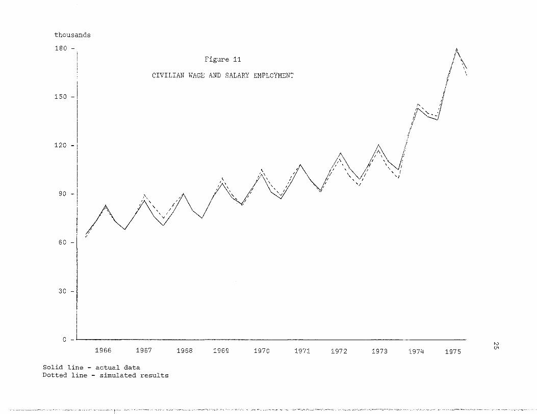
Historical simulations have been run for the 1966:1 to 1975:4
period, years of rapid but uneven growth in the Alaska economy,
culminating with a sharp spurt induced by pipeline construction,
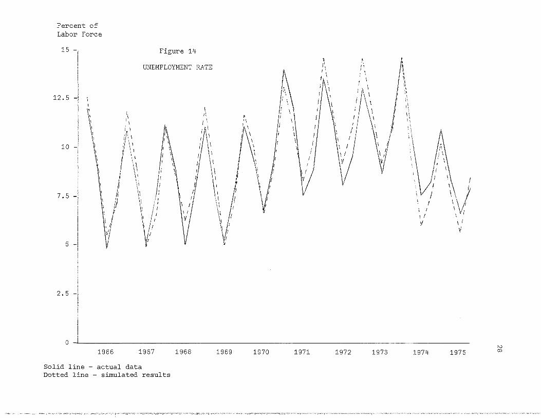
Figures 11 to 15 graph the simulated results for the historical
period against the actual data, for five key variables in the model.
Table 1 lists the measures of "goodness of fit" for each variable
determined within the model. These measures can show how well the
model "tracks" the historical period,
The true test of a forecast model, however, is its ability to
forecast beyond the historical data. The preliminary data for 1976:1
and 1976:2 (see Figures 1-9) indicate that the model can pass this
most rigorous test.
thousands
180 -
150 -
120 -
90 -
:,
60 -
30 -
,,,_ IA ,
Figure 11
CIVILIAN WAGE AND SALARY EMPLOYMENT
' I I
' V
,, '·\
\ ,, ~ I,/
If '1
\
,A' ' \
' ' I ' / V,
/
'
1 I,
I'- \JI
/:\ ' I
I
V
',V/ ' I ' I ' '/ J
I,
1, /,
A
o-~------------------------------------------1966 1967
Solid line - actual data Dotted line - simulated results
1968 1969 1970 1971 1972 1973 1974 1975 tv (J1

Millions of dollars
450 -
375 -
300 -
225 -
150 -
75 -
Figure 12
REAL DISPOSABLE PERSONAL INCOME
(Seasonally Adjusted)
~---- "'~ ... /
, , /
/
/
/
/1
~
~ ,,
I f,
/,
,.. I
0 ---------------------------------------------------------1966 1967
Solid line - actual data Dotted line - simulated results
1968 1969 1970 1971 1972 1973 1974 1975 rv Ol

(1967=142.5)
240 -,
200 -
160 -
~7
120 -
80 -
40 -
Figure 13
ALASKA RELATIVE PRICE INDEX
---
0------------------------------------------1966 1967 1968
Solid line - actual data Dotted line - simulated results
1969 1970 1971 1972 1973 1974 1975 l'0 --.J
Percent of Labor Force
15 - Figure 14
UNEMPLOYMENT RATE
12. 5 -I \ I
\1 1 I
10 -
7.5 -
5 -
2.5 -
0
1966 1967
Solid line - actual data Dotted line - simulated results
,,
1968 1969
i t \\
'
\
\\ I
I \
1970 1971
I
I
1972 1973
I I \
\ I I
I
ll V
1974 1975 "" co

thousands
30 -
25 -
20 -
15 -
10 -
5 -
·, /
Figure 15
TRADE EMPLOYMENT
,,,,._ ,,-_ /~..._·" -~// '
I '- ./' \ I '\
/
" ;, \ I '\.I ~~ \ I I .,;
- ,,;-~-, /' I-, /"/ ' ~ ' " ' / /
I
I~ ,, I
I 1, ·
o-~----------------------------------------1966 1967
Solid line - actual data Dotted line - simulated results
1968 1969 1970 1971 1972 1973 1974 1975
1')
lO
ALASKA ECONOMIC FORECAST FOR 1977
APPENDIX
Daniel A. Seiver Institute of Social and Economic Research
University of Alaska 707 "A" Street, Suite 206 Anchorage, Alaska 99501
March 2, 1977

Alaska Economic Forecast for 1977
APPENDIX
1. Model Equations
2. Stochastic Regressions

u .I"\+ ~. 3:
4: c:· + .J.
(.d
7:
a: q+ ' .
:I. 0:
1:1.:
1 '"). ~· 1. 3:
:L 4:
l 5 !
1. Model Equations
RPIQ = CRPIA+CRPIB*PCC-1)+CRPIC*DELC4 : DPIRQS)tCRPID*RPIQ(-1.)
PI1Q == 1+33718*WS99Q**0.98361
PIQ == PI1QtDNCSQ
PIBARQ == PIQ*lOO./RPIQ
DPIQ ==-EXPC0.30764+0.93156*LOGCPIQ))
DPIRQ == lOO*DPIQ/RPIQ
DPIRQS = DPIRQ/SFAC
LOG(WRM8Q) = CM8WA+CM8WB*LOGCWEUSQ)tCM8WC*S1+CM8WD*S2+CM8WE*S3+CM8WF*<ECONXQ/EMCNQ)
WSMBQ == EMMBQ*WRMBQ
LOGCWRGFQ) = CGFWA+CGFWB*LOGCWEUSQ)
WSGFQ == EMGFQ*WRGFQ
LOGCWRP9Q) = CP9WA+CP9WB*LOG<WEUSQ)tCP9WC*S1.tCP9WD*S2tCP9WE*S3+CP9WF*<ECONXQ/EMCNQ)
WSP9Q == EMP9Q*WRP9Q
LOGCWRA9Q) = CA9WAtCA9WB*LOGCWEUSQ)tCA9WC*S1tCA9WD*S2tCA9WE*S3
WSA9Q == EMA9Q*WRA9Q

16:
:L 7 !
18:
19!
20:
:~~ :I. :
'J"J + Ao.,. .. ,0,
~.~3:
~-~4:
"")r::" .. .a.~.,J f
:~6:
27:
~~8:
:~~9:
;30:
31:
32:
~53:
EMCMQ = CCMA+CCMB*DPIRQS+CCMC*DUMMY
LOGCWRCMQ) = CCMWA+CCMWB*LOG(WEUSQ)+CCMWC*S1+CCMWD*S2+CCMWE*S3+CCMWF*CECONXQ/EMCNQ)
WSCMQ == EMCMQ*WRCMQ
EMPUQ = CPUA+CPUB*DPIRQS+CPUC*S1+CPUD*S2+CPUE*S3
LOG(WRPLJQ) = CPUWA+CPUWB*L0G(WEUSQ)+CPUWC*S1+CPUWD*S2+CPUWE*S3+CPUWF*CECONXQ/EMCNQ)
WSPUQ == EMPUQ*WRPUQ
LOG(WRFIQ) = CFIWA+CFIWB*LOGCWEUSQ)+CFIWC*S1+CFIWD*S2+CFIWE*S3+CFIWF*CECONXQ/EMCNQ)
EMFIQ = CFIAtCFIB*DPIRQS+CFIC*DPIRQS**2
WSFIQ == EMFIQ*WRFIQ
EMCN1Q = CCNAtCCNB*DPIRQStCCNC*S1+CCNE*S3+CCNF*BOOM
LOG(WRCNQ) = CCNWA+CCNWB*LOGCWEUSQ)tCCNWC*S1+CCNWD*S2tCCNWE*S3+CCNWF*CECONXQ/EMCNQ)
EMCNQ = EMCNlQ+ECONXQ
WSCNQ == EMCNQ*WRCNQ
EMMOQ = CMOA+CMOB*DPIRQStCMOC*S1+CMOD*S2tCMOE*S3tCMOF*DPIRQS**2
LOGCWRMOQ) = CMOWAtCMOWB*LOGCWEUSQ)tCMOWC*S1tCMOWE*S3tCMOWF*CECONXQ/EMCNQ)
WSMOQ == EMMOQ*WRMOQ
EMD9Q = CD9AtCD9B*DPIRQStCD9C*S1tCD9E*S3+CD9F*DPIRQS**2
LOGCWRD9Q) = CD9WA+CD9WB*LOGCWEUSQ)tCD9WC*S1+CD9WD*S2+CD9WE*S3+CD9WF*(ECONXQ/EMCNQ)
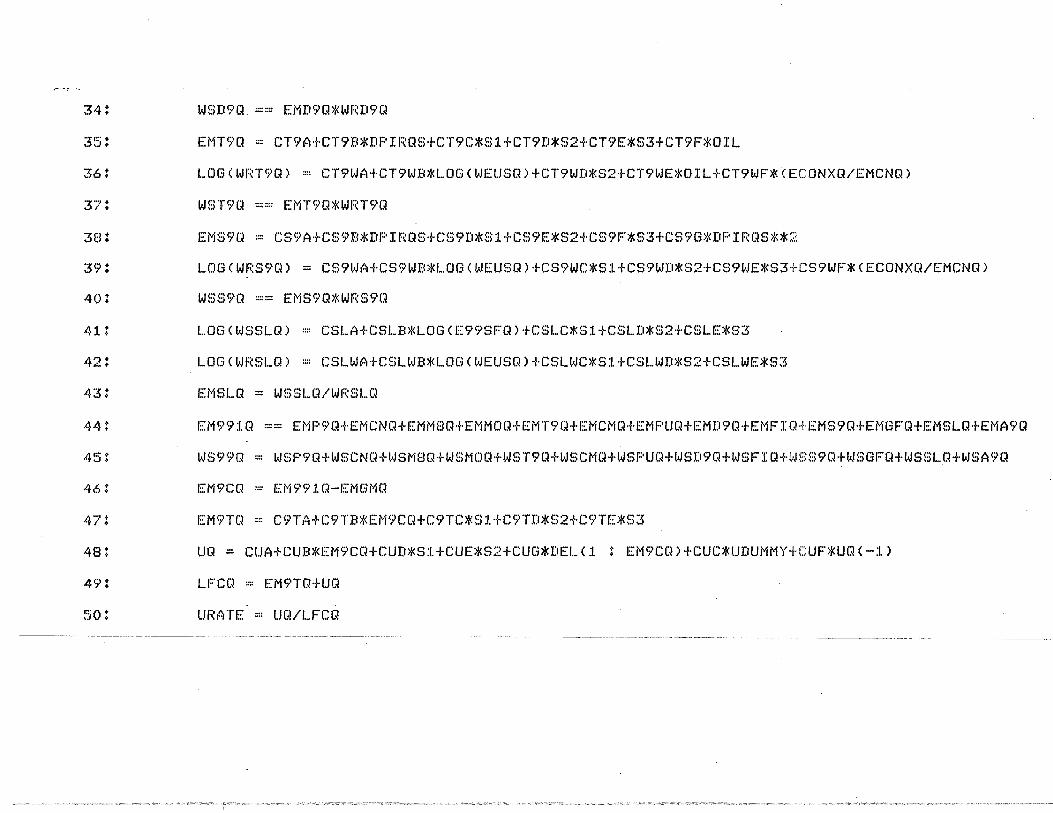
34!
:55 !
36:
37:
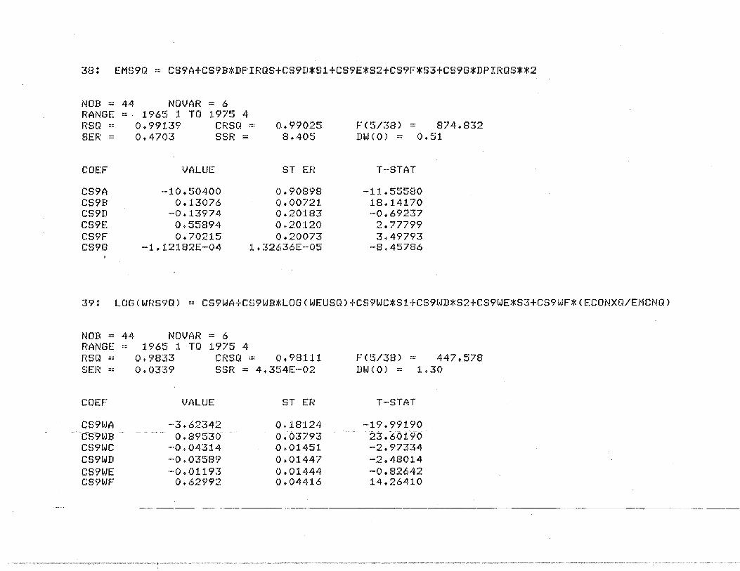
3B:
39:
40:
41:
42:
43!
44!
45:
46t
47:
48:
49!
50!
WSD9Q. == EMD9Q*WRD9Q
EMT9Q = CT9AtCT9B*DPIRQStCT9C*S1tCT9D*S2tCT9E*S3tCT9F*OIL
LOG(WRT9Q) = CT9WA+CT9WB*LOGCWEUSQ)tCT9WD*S2tCT9WE*OIL+CT9WF*CEC0NXQ/EMCNQ)
WST9Q == EMT9Q*WRT9Q
EMS9Q = CS9AtCS9B*DPIRQStCS9D*S1+CS9E*S2+CS9F*S3tCS9G*DPIRQS**2
LOGCWRS9Q) = CS9WA+CS9WB*LOGCWEUSQ)tCS9WC*S1tCS9WD*S2+CS9WE*S3+CS9WF*CECONXQ/EMCNQ)
WSS9Q == EMS9Q*WRS9Q
LOGCWSSLQ) = CSLA+CSLB*LOGCE99SFQ)tCSLC*S1tCSLD*S2+CSLE*S3
LOGCWRSLQ) = CSLWA+CSLWB*LOGCWEUSQ)tCSLWC*S1tCSLWD*S2tCSLWE*S3
EMSLQ = WSSLQ/WRSLQ
EM991Q == EMP9QtEMCNQ+EMM8QtEMM0QtEMT9QtEMCMQtEMPUQtEMD9QtEMFIQ+EMS9QtEMGFQtEMSLQtEMA9Q
WS99Q = WSP9QtWSCNQtWSM8QtWSM0QtWST9QtWSCMQtWSPUQ+WSD9QtWSFIQtWSS9QtWSGFQtWSSLQtWSA9Q
EM9CQ = EM991Q-EMGMQ
EM9TQ = C9TAtC9TB*EM9CQtC9TC*S1tC9TD*S2tC9TE*S3
UQ = CUA+CUB*EM9CQtCUD*S1tCUE*S2tCUG*DEL(1 : EM9CQ)tCUC*UDUMMYtCUF*UQ(-1)
LFCQ = EM9TQtUQ
URATE = UQ/LFCQ ---~------

·-- ····---.
l)Af~ I ,~BLEfl U!:;ED IN EW.JATIONS DF'IQ ~) 6 DF'IF~Q 6 7 DF'IRC~S j_ 7 16 :I. 9 23 r)I:-:"
.:.....J 29 32 35 38 EMCMC~ 11.i 18 44 EMCNQ 8 :1.2 17 20 :~2 26 27 28 30 33 ~56 39 44 EMCN:I.() ··1 "" h<. ,.,
.... ) .... •... I
EMD9() :3::.~ ~54 44 EMF IC~ ..• , .. r
,:~,:) 24 .44 EMMOC~ 2s> 31 44 EMF'UQ 19 21 44 EMSLQ 4··· ~'> 44 EMS9C~ :rn 40 44 EMT9Q 3~) :o 44 EM9CC~ 461 47 48 EMS1TC~ 47 49 EM991Q 44 46 LFCC~ 49 :50 P :r n,~r~t~ 4 PIC~ ;3 4 5 PI1Q =~ 3 1:~p:r (~ j_ 4 6 LIQ 48 49 50 URATE 50 l,,.IF~t19C~ 14 j_ 5 f,JF~CMC~ :1.7 18 WRCNC~ 26 28 l,,.lfU:,9(~ 33 34 J..JF~F I(~ ;1~~ 24 WFWFC~ :I. 0 1.1 tJRMOC~ 30 31 Wl:::MBC~ 8 9 WF~Pl.JC~ 2() 21 wr.;:p9Q 1 ':> - 13 WRSL.Q 4::_~ 43 w1:;:s9Q 39 40 t,JRT9Q :,6 37 WSA9l~ 1 ~) 45 J.JSCMC~ :l8 45 WSCN() 2f:l 45 WSD9C~ ;·54 45 WSFH1 24 45 WSC·JFC~ U. 45 WSMOQ 3:1.' 45 J..J!:;MBC~ 9 45 l..JSPLJt~ 21 45 WSF'9Q 13 45 J..JS!:il..Q 41 43 45 I..JSS9C~ 40 45 WST9Q 37 45 WS99Q ;! 45
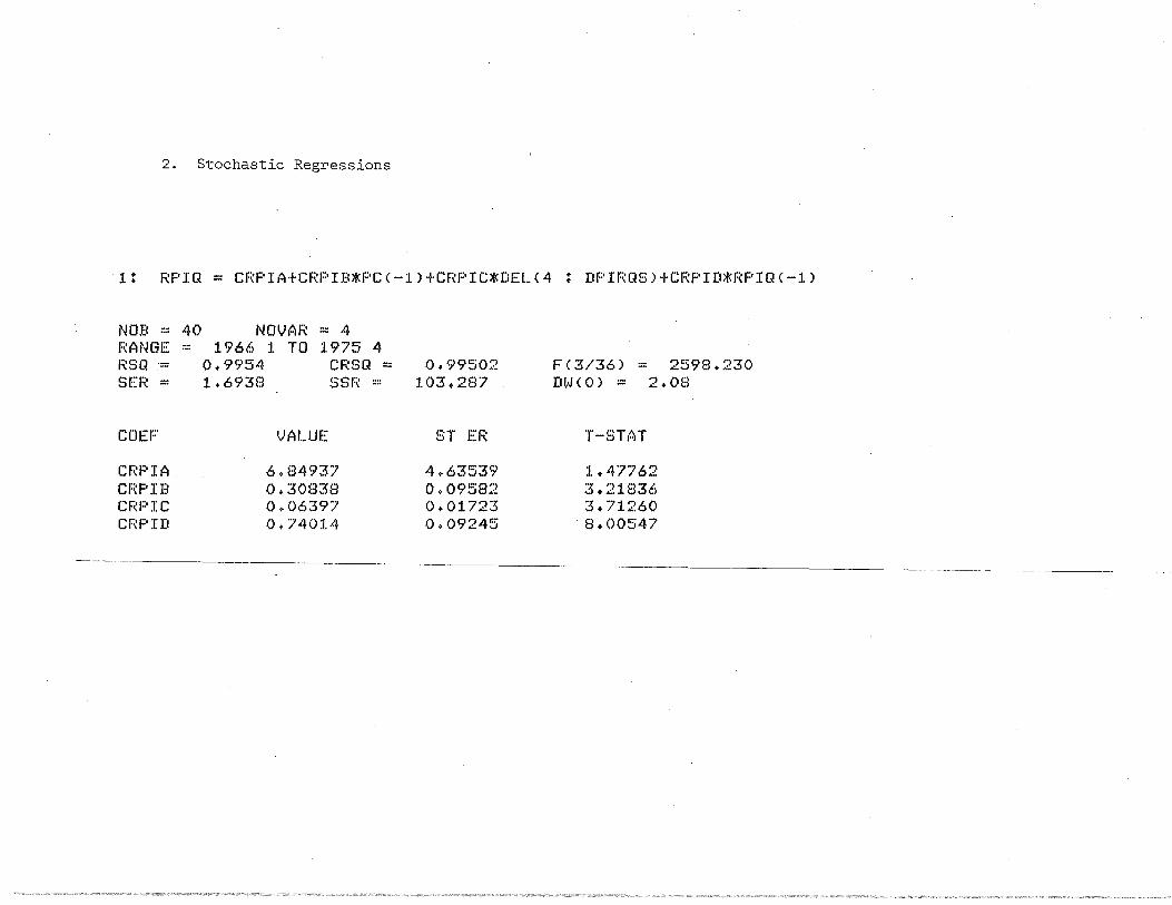
2. Stochastic Regressions
1: RPIQ:::: CRPIA+CRPIB*PC(-1)tCRPIC*DEL(4 : DPIRQS)tCRPID*RPIQ(-1)
NOB :::: 4() NOVAF~ == 4 RANGE 0-~ 1966 1 TO 1975 4 l=i:SQ .== 0+9954 CRSQ == SE!=~ == :r. .6938 SSR :::
COEF VALUE
CRPIA 6.84937 CRPIB 0.30838 CRPIC (). 06>397 cr=~PID o. 740:1.4
0. 99!:'j02 103+287
ST Ef~
4 + 6:~5:~9 0+09582 0+01723 0+09245
FC3/36):::: 2598.230 DW < 0) ::: 2. 08
T-·STAT
:J..47762 3+21836 3+71260 8.00547
--- - "----~---

a: LOGCWRMBQ) = CM8WA+CM8WB*LOGCWEUSQ)tCM8WC*S1+CM8WD*S2+CM8WE*S3tCM8WF*<ECONXQ/EMCNQ)
NOB= 44 RANGE= RSQ = SER=
COEF
CM8WA CM8WB CMBWC CM8WD CM8WE CM8WF
NOVAR = 6 1965 1 TO 1975 4
0.91411 CRSQ = 0. 0t°>05 S[")f:! -
VALUE
-3.2()933 ().86196
-().06185 -0.()3274
0+02758 ().18617
0.9028:1. 0.139
ST EF~
0.32403 0.06782 0.02594 0+02587 0 • 0258 :I. 0 • 07B9~'i
10: L.OGCWRGFQ) = CGFWA+CGFWB*LOGCWEUSQ)
NOB= 44 NOVAR = 2 RANGE= 1965 :L TO 1.975 4 RSQ = 0.96773 CRSQ = 0+96696 SER= 0+0474 SSR = 9+42()E-02
COEF
CGFWA CGFWB
VALUE
-6.()1295 -1.+39726
ST EF~
0.18934 o. o:~937
F(5/38) -DW<O> =
T-STAT
1.83
·-·9. 90430 12.70980 -2.38452 --:L. 26521
1+06881. 2,35804
8() + 88B
F(l/42) = 1259+600 DW(O) = 0.44
T-STAT
-3:L.75710 35.4906()

12: LOG<WRP9Q) = CP9WAtCP9WB*LOGCWEUSQ)tCP9WC*S1+CP9WD*S2tCP9WE*S3tCP9WF*CECONXQ/EMCNQ)
NOB= 44 NOVAR = 6 RANGE= 1965 1 TO 1975 4 RSQ = 0.9499 CRSQ = SER= 0.0593 SSR =
COEF VALUE
CP9WA -3+58452 CP9WB 1+05648 CP9WC -0.04699 CP9WD -0.09489 CP9WE -0.08967 CP9WF 0+38794
0.94331 0.134
ST ER
0.31761 0.06647 0+02542 0+02536 0.02530 0.07739
FC5/38) = 144.109 DW(O) = o;69
T-STAT
-11+28600 15.89330 -1.84839 -3.74164 -3.54500
5+01297
14 t LOG< WR1~9C~) :::: CA9WA+CA9WB*LOG < WEUSQ) +CA9WC*S1. +CA9WD*S2+CA9WE*S~5
NOB= 44 RANGE "" RSQ -·
-SE1=~--=
COEF
CA9WA CA9WB CA9WC CA9WD CA9WE
NDVAR == 5 196!:'i 1 TO :L 975 4
0+75823 CRSQ = o. :1~aHi-- - ··ss,~-;;
V.:~LUE
--!:'i + 66450 1+42204
-0.26813 ····O. 1. 9630
0.0~545:L
0.73344 1.289
ST ER
0 + 736:33 0+15209 0.07790 0.07766 0.07751
FC4/39) = 30.578 -----DWCO> -:;:;--1..:'f"i
T-STAT
··-7+69289 9+35031
·-3 + 44217 -2.52788
o.70323
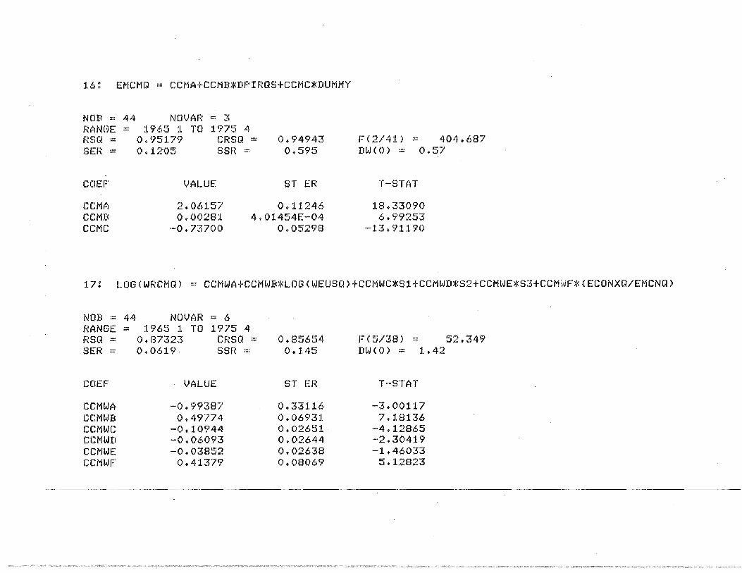
16: EMCMQ = CCMA+CCMB*DPIRQS+CCMC*DUMMY
NOB= 44 RANGE= RSQ = SER=
COEF
CCMA CCMB CCMC
NOVAR = 3 1965 1 TO 1975 4
0.95179 CRSQ = 0.94943 0. ~595 0.1205 SSR =
VALUE ST ER
2+06157 0.11246 0.0028:L 4. 01454E···04
·-0. 73700 0.05298
FC2/41) = 404.687 DWCO> = 0.57
T-STAT
18.33090 6.99253
-13+91190
17: LOG(WRCMQ) = CCMWA+CCMWB*LOGCWEUSQ)tCCMWC*S1+CCMWD*S2tCCMWE*S3tCCMWF*CECONXQ/EMCNQ)
NOB= 44 NOVAR = 6 RANGE= 1965 1 TO 1975 4 RSQ = 0+87323 CRSQ = SER= 0.0619 SSR =
COEF · VALUE
CCMWA -0.99387 CCMWEi 0.49774 CCMWC ·-0 .1.0944 CCMWD -·O. 06093 CCMWE -o. 0'.3852 CCMWF ().41379
0.85654 0+145
ST ER
0.331:t.6 0.()6931. 0+02651 0.02644 0.02638 0+08069
F(5/38) = 52.349 DWCO) = 1+42
T·-STAT
--3.00117 7 .1.8136
-4.1.2865 ·-2 + 30419 -1.46033
5+12823

19: EMPUQ = CPUA+CPUB*DPIRQS+CPUC*S1+CPUD*S2+CPUE*S3
NDB == 44 RANGE a::
1=~st1 ,.:: SER=
COEF
CPUA CPUB
-'"-CPD C - -CPUD CPUE
NOVAR == !'.'i 1965 1 TD 1975 4
0+80744 cr~sQ = 0.78769 o. o7:rn SSR = 0.208
VALUE ST ER
o.40249 0.04453 0+00205 1.68621E-04
- .... ().04922 ·- . 0.0313:t ~0.01203 0+03122
0+03744 0+03116
F(4/39) = 40.884 DW(O) = 0+23
T-·STAT
9.03907 12+1.7890 -1+57148 -0+38524
1+20133
20: LOG(WRPUQ) = CPUWA+CPUWB*LOG(WEUSQ)+CPUWC*S1+CPUWD*S2+CPUWE*S3+CPUWF*<ECONXQ/EMCNQ)
NOB= 44 RANGE= RSQ = SER=
COEF
CPUWA CPUWB CPUWC CPUWD CPUWE CPUWF
NOVAR = 6 l.965. 1 TO l.975 4
0.98325 CRSQ = 0+98104 0+0350 SSR = 4.652E-02
VALUE
-4.05653 1.10120
-0.03379 -0.04658 ~0.02279
0+41334
ST EF~
0 + 187:B 0+0392:L 0+01500 0.01496 0+01492 0 + 04!564
FC5/38) = 446.102 DWCO) = 2+00
T--STAT
--21 + 65420 28.08650 ·-2.25365 ·--~~+11.401 -1+52770
9+05570

22! LOG(WRFIQ) = CFIWA+CFIWB*LOG(WEUSQ)tCFIWC*S1tCFIWD*S2tCFIWE*S3tCFIWF*<ECONXQ/EMCNQ)
NOB= 44 NOVAR = 6 RANGE= 1965 1 TO 1975 4 RSQ = 0.98476 CRSQ = 0+98275 SER= 0.0246 SSR = 2+301E-02
COEF VALUE ST ER
CFIWA -3.64423 0+13175 CFIWB 0.94031 0.02757 CFIWC -0+05619 0.01055 CFIWD -0.07232 0.01052 CFIWE -0.08505 0+01049 CFIWF 0+08544 0.03210
F(5/38) = 490.924 DW(O) ::::. :l.+48
T-.. STAT
·-27. 6~'5970 34 + :J.0010 -5.32784 ·-6+87461 -.. 8 .10496
2+66137
23: EMF IC~ ::: C-FIA+CFIB*DPIFWS+CFIC*DPHWS**2
NOB= 44 RANGE ·,=~SQ .... SER :::
COEF
CFIA CFIB CFIC
NOVAR = 3 1965 1 TO 1975 4
0.96008 CRSQ = 0.9!:'i813 2+635 () • 253!'5 SSR ....
VALUE
-2+15244 0+03082
--2 + 3541. OE--05
ST ER
0+48667 0.00388
7 + 14:1. 72E-06
F(2/41) = 492.964 DW(O) = 0+62
T-·STAT
--4 + 42280 7+93641
-3.29626
- ---· . - - ----···

25: EMCN1Q = CCNA+CCNB*DPIRQStCCNC*S1tCCNE*S3tCCNF*BOOM
NOB == 44 NOVAR ::: 5 RANGE ::: 1965 1 TO 1975 4 1:;:SQ :::: 0+97882 CF~SQ ::., £>EH == 0 + 488:3 SSR ::::
COEF . V1qLUE
CCNA 2.:33448 CCNB 0+02339 CCNC -2.76581 CCNE 2+47366 CCNF 2.67796
0.97665 9+300
ST D1
0 + 4:~995 0.00:~12 0+18101 0 + 1.8128 0+40664
F(4/39):::: 450+651 DW<O> =-0 1 +40
T--STAT
5.30621 U.+01840
-15.27990 13.64570
6 + 585!55
26: LOGCWRCN~) = CCNWAtCCNWB*LOGCWEUSQ)tCCNWC*S1tCCNWD*S2tCCNWE*S3tCCNWF*CECONXQ/EMCNQ)
NOB= 44 RANGE= RSQ = SER=
COEF
CCNWA CCNWB CCNWC CCNWD CCNWE CCNWF
NOVAR:::: 6 1965 1 TO 1975 4
0+95606 CRSQ = 0+0658 SSR =
VALUE
·-2.47747 0.83080
--0 + 10912 -0.05986
0.()~5591 0. 9<!')404
0.95028 0+164
ST ER
0.35209 0.07369 0.02818 0+02811 0+02804 0+08579
FC5/38) -DW(O) =
T-STAT
165.372 1+09
-·7 + 03655 11+27430 -3.87164 ·-2. 12928
1+28055 :L1 +23760

29: EMMOQ = CM0AtCMOB*DPIRQStCMOC*S1tCMOD*S2tCMOE*S3tCMOF*DPIRQS**2
NOB= 44 RANGE= RSQ = SER=
COEF
CMOA CMOB CMOC CMQD CMOE CMOF
NOVAR = 6 1965 1 TO 1975 4
0.96686 CRSQ = 0.9625 0.0682 SSR = 0+177
VALUE ST El:~
-0+92:1.63 0+1.3178 0 + 014~:i!:'i 0.00104
-0.11649 o. 02<?26 0+08869 0.02917 9. 14528 0.02910
-1.83648[-05 1+92295E-06
FC5/38) = 221+728 DWCO) = 0+86
T-STAT
-··6 + 9<9~549 :1.3. 92760 -3.98113
3+04032 4+99205
--9 + 55029
30: LOGCWRMOQ) = CMOWAtCMOWB*LOG(WEUSQ)tCMOWC*S1tCMOWE*S3tCMOWF*<ECONXQ/EMCNQ)
------i;n:rri-==-44 ___ -- NOVM~ = ~i
RANGE= 1965 1 TO 1975 4 ,=ma .. _ SEF~ =
(). 95828 0.0473
CRSQ = 0.954 SSR = 8.711E-02
COEF VALUE ST ER
CMOWA .... 3. 50690 0+25147 CMOWB 0+94916 0+05283 CMOWC --(). 07327 0+01752 CMOWE 0.04389 0+01746 CMOWF 0+29:1.49 0+06161
FC4/39) = 223.954 DW(O) ::: 1 .• 27
T-STAT
.. -:1.3 + 94540 17+96790 ·--4. 18204
2+51356 4+73100
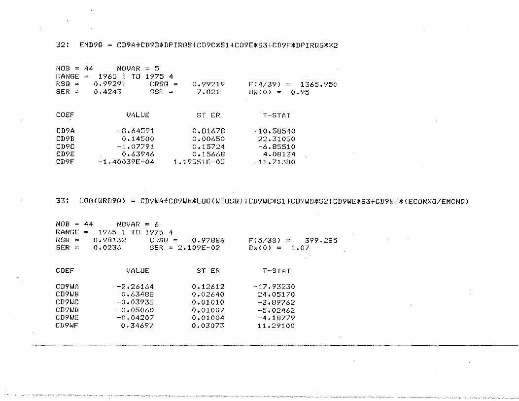
32: EMD9Q = CD9AtCD9B*DPIRQStCD9C*S1tCD9E*S3tCD9F*DPIRQS**2
NOB= 44 RANGE= RSQ = SER=
COEF
CD<JA CD9B CD9C CD9E CD9F
NOVAR = 5 1965 i TO 1975 4
0.99291 CRSQ = 0.99219 0.4243 SSR = 7.021
VALUE ST ER
-·8. 6459:L 0+81678 0+145()0 0 + 006~i0
·-1 .07791 0.15724 0.63946 0+15668
-.. 1. 400:~9E--04 1. + l 9!:i51E-05
FC4/39) = l365.950 DWCO) = 0+95
T .. ··STAT
--10+58540 22.31050 -6.85510
4.08134 -··11 + 71380
33: LOGCWRD9Q) = CD9WA+CD9WB*L0G(WEUSQ)tCD9WC*S1+CD9WD*S2tCD9WE*S3+CD9WF*CECONXQ/EMCNQ)
NOB= 44 RANGE :::: F.:SQ == SER ca:
COEF
CD9WA CD9WB CD9WC CD9WD CD9WE CD9WF
NOVAR = 6 1965 l TO 1975 4
0.98132 CRSQ = 0.97886 0+0236 SSR = 2+109E-02
VALUE
-2.26164 0.63488
-0.03935 -0.05060 -0.04207
0.34697
ST El:.:
0+126:1.2 0.02640 0.01010 0.01.007 0+01004 0.03073
FCS/38) -DWCO) =
T-·STAT
399+285 1+07
-17+93230 24+05170 -3.89762 -5.02462 -4.18779 1.1 .• 291.00

35: EMT9Q = CT9A+CT9B*DPIRQStCT9C*S1+CT9D*S2tCT9E*S3+CT9F*0IL
NOB= 44 RANGE= RSQ~ SER=
COEF
CT9A CT9:£! CT9C CT9D CT9E CT9F
NOVAR = 6 1965 1 TO 1975 4
0.98296 CRSQ = 0+98072 0.2961 SSR = 3+332
. VALUE ST ER
O+l.5475 0+19582 0+02729 8.35889E-04
··-0. 53098 0 + 12733 0+43527 o. l.2c>69 0+96244 0+12639 o.74263 0+12658
F(5/38) = 438+521 DW(O) == 0.98
T--STAT
0.79026 32+65070 -4.17019
3.43577 7. 61!509 5+86677
36: LOGCWRT9Q) = CT9WA+CT9WB*LOGCWEUSQ)tCT9WD*S2tCT9WE*OIL+CT9WF*CECONXQ/EMCNQ)
NOB= 44 NOVAR = 5 RANGE= 1965 1 TO 1975 4 RSQ = 0.97776 CRSQ = 0.97547 SER= 0+0435 SSR = 7+371E-02
COEF VALUE ~n E(:;;
CT9WA -~5. 67630 0+23145 CT9WB 0. <J6782 0.04859 CT9WD ····0+03998 0+01529 CT9WE 0+05552 0+01953 CT9WF 0+66875 0.06622
F(4/39) = 428.575 DWCO) = 1.12
T-STAT
-15+88380 :I. 9 + 91940 -2.61428
2+84257 10+09880
~-··---··~
38: EMS9Q = CS9AtCS9B*DPIRQStCS9D*S1tCS9E*S2tCS9F*S3tCS9G*DPIRQS**2
NOB ::., 44 RANGE= RS(~ = SER=
COEF
CS9A CS9B CS9D CS9E CS9F CS9G
NOVAR ~-= 6 1965 1 TO 1975 4
0.99139 CRSC~ ::: 0+99025 0+47()3 SSF~ == 8+405
VALUE ST ER
-1. 0. ~';0400 ().90898 () + 1.3076 0+0072:1.
--() +13974 0.20:183 0+55894 0.20120 0+70215 0 + 2007:5
--1.. 12Hl2E-·04 1.. :'>2636E-··05
F(5/38) = 874.832 DWCO) = 0.51
T--STAT
-11 .• 55580 1.8 + 1.4170 -0.69237
2+77799 3+49793
--8 + 45786
39: LOG(WRS9Q) = CS9WA+CS9WB*LOGCWEUSQ)tCS9WC*S1tCS9WD*S2tCS9WE*S3+CS9WF*CECONXQ/EMCNQ)
NOB= 44 NOVAE'. • .,, 6 1:;;ANGE == 1.965 1 TO 1975 4 RSC~ :::: ().9833 CF~SC~ == 0+9811.:l ~:1ER == o. o:'>~~9 SSR = 4 + 354E .. -02
COEF VALUE
CS9WA -3.62342 -·-c.s9WB - - - -- -- 0 + 895:50- - .
CS9WC -0.04314 CS9WD -0.03589 CS9WE -0.01193 CS9WF 0+62992
ST ER
0.18124 0+03793 0+01451 0+01447 0+01444 0+044:1.6
FC5/38) = 447.578 DWCO> = 1.30
T-STAT
·-·19. 99190 23+60190 -2.97334 .. -2.48014 -0.82642 14+26410

41: LOG<WSSLQ) = CSLAtCSLB*L0G(E99SFQ)tCSLC*S1tCSLD*S2tCSLE*S3
NOB= 44 RANGE= RSQ -SER=
COEF
CSLA CSLB CSLC CSLD CSL£
NOVAR = 5 1965 ·1 TO 1975 4
0.9806 CRSQ = 0.0728 ~)Sf~ --
VALUE
-0.86161 0+86122
-0.00282 ·0.05730
-0.03952
0.97861 0.206
ST ER
0+11074 0.01951 0+03119 0.03119 0.03103
FC4/39) -DWCO) =
492.932 1. 16
T-STAT
-7.78029 44+13200 -0.09052
1.83702 -1.27366
42: LOG(WRSLQ) = CSLWAtCSLWB*LOG(WEUSQ)tCSLWC*S1tCSLWD*S2tCSLWE*S3
NOB= 44 NOVAR = 5 RANGE= 1965.1 TO 1975 4 RSQ = 0.9713 CRSQ = 0.96835 SER= 0.0390 SSR = 5+937£-02
COEF VALUE ST ER
CSLWA -4.71968 0+1!:"i806 CSLWB 1+17888 0.03265 CSLWC --O.OO:L72 0.01672 CSLWD -·O. 00300 0.01667 CSLWE .. :.0.04200 0.01664
FC4/39) = 329+916 DWCO) = 1+34
T--STAT
··-29 + 85960 36.11000 -0.10308 -0.18012 -2.57730
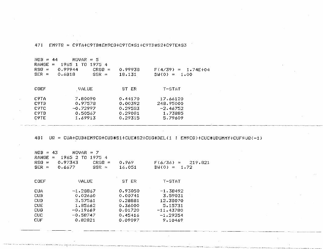
47: EM9TQ = C9TAtC9TB*EM9CQtC9TC*S1tC9TD*S2tC9TE*S3
NOB == 44 NOVAR ::: 5 l,:ANGE === 196!':'i 1 TO :l 975 4 RSQ •-= 0.99944 CF~SQ == SEF~ = 0+6818 Sf31:~ :::
COEF VALUE
C9TA 7+80090 C9TB 0+97578 C9TC --0 + 72997 C9TD 0.50567 C9TE 1.69913
0+99938 1s.1:n
ST EF~
0+44170 0+00392 0+29583 0+29081 0.29315
FC4/39) = 1+74Et04 DWCO) = 1+00
T-STAT
17.66120 248.95000
--2 + 46752 1.73885 5.79609
48: UQ = CUA+CUB*EM9CQtCUD*S1tCUE*S2tCUG*DEL(1 : EM9CQ)tCUC*UDUMMYtCUF*UQC-1>
NOB= 43 NOVAR = 7 RANGE= 1965 2 TO 1975 4 RSQ = 0.97343 CRSQ = SER= 0.6677 SSR =
COEF VALUE
CUA --1.28867 CUB 0.02660 CUD 3.57~56:t. CUE :l .• 85662 CUG ···O + 19669 CUC --0. 58747 CUF 0.82821
0.969 16.051
ST EF~
0.93050 0.00741 0+28881 0.36000 0.01720 0.45416 0.09097
FC6/36) = 219+821 DWCO> = 1+72
T·-STAT
···1+ 38492 3+59031
12+38070 5+15731
-1. l. + 43780 --1 +29354
9.10469


