AlbertEinsteinInstitute,AmMühlenberg1,D … · 2 C. F. PAGANINI, B. RUBA AND M. A. OANCEA 1....

CHARACTERIZATION OF NULL GEODESICS ON KERRSPACETIMES

CLAUDIO F. PAGANINI†, BLAZEJ RUBA‡ AND MARIUS A. OANCEA∗

†Albert Einstein Institute, Am Mühlenberg 1, D-14476 Potsdam, Germany

‡Faculty of Physics, Astronomy and Computer Science, Jagiellonian University,Lojasiewicza 11, 30-348 Cracow, Poland

∗Faculty of Physics, Babes-Bolyai University, 400084, Cluj-Napoca, Romania

Abstract. We consider null geodesics in the exterior region of a sub-extremalKerr spacetime. We show that most well known fundamental properties of nullgeodesics can be represented in one plot. In particular, one can see immediatelythat the ergoregion and trapping are separated in phase space.Furthermore, we show that from the point of view of any timelike observeroutside of a black hole, trapping can be understood as a smooth sets of spacelikedirections on the celestial sphere of the observer.

Contents

1. Introduction 2Overview of this paper 32. The Kerr Spacetime 32.1. Symmetries and Constants of Motion 43. Geodesic Equations 63.1. The Radial Equation 63.2. The θ Equation 94. Special Geodesics 94.1. Radially In-/Out-going Null Geodesics 94.2. The Trapped Set 104.3. T-Orthogonal Null Geodesics 125. Trapping as a Set of Directions 135.1. Framework 145.2. The trapped sets in Schwarzschild 145.3. The trapped sets in Kerr 156. Application 21Acknowledgements 22Appendix A. 22References 23

E-mail address: [email protected], [email protected],[email protected].

Date: October 19, 2017 File:Kerrnullgeod.tex.1

arX

iv:1

611.

0692

7v3

[gr

-qc]

18

Oct

201

7

2 C. F. PAGANINI, B. RUBA AND M. A. OANCEA

1. Introduction

In recent years there has been a lot of progress in the Kerr uniqueness and theKerr stability problem. Having a thorough understanding of geodesic motion and inparticular the behavior of null geodesics in Kerr spacetimes is helpful to understandmany of the harder problems related to these spacetimes. In this paper we studythe properties of null geodesics in the exterior region in the sub-extremal case,where a ∈ [0,M). The geodesic structure of Kerr spacetimes has been subject ofa lot of research. Our aim here is to give a unified and accessible presentation ofthe most important properties of geodesics in the Kerr spacetime, with regard tothe open problems mentioned above. The Mathematica notebook that has beendeveloped for this paper is intended to help the reader gain an intuition on theinfluence of various parameters on the geodesic motion, despite of the complexityof the underlying equations. It can be downloaded under the permanent link [1].In Section 6 we explain where these plots give useful insights.

An extensive discussion of geodesics in Kerr spacetimes and many further refer-ences can for example be found in [4, p.318] and [15]. See [19] for a nice treatmentof the trapped set in Kerr including many explicit plots of trapped null geodesicsat different radii. Here we focus more on global properties of the null geodesics andless on the details of motion. Analyzing the turning points for a dynamical system isa powerful tool to extract information about its global behaviours. For example, inany 1+1 dimensional system stable bounded orbits only exist if there exist two dis-joint turning points in the spacial direction between which the system can oscillate.For geodesics in Kerr this has been studied in detail by Wilkins [20]. The techniquesused here are very close to that paper. Many of the results discussed in the first foursections of this note are in fact well known, however our focus is on proving that allthese properties can be read of from one simple plot. Thereby making it easier forpeople to understand the general behaviour of null geodesics in Kerr. Hence we doshow that the various plots provided in the notebook actually do cover the wholespace of relevant parameters. A different representation of the forbidden regions inphase space can be found in [15, p.214] and also in [17]. The presentation chosenhere is adapted to help understand the phase space decomposition used in the prooffor the decay of the scalar wave in subextremal Kerr [7].

The novel material in this note which is presented in the section 5 is relatedto the notion of black hole shadows. The shadow of the black hole is defined asthe innermost trajectory on which light from a background source passing a blackhole can reach the observer. The first discussion of the shadow in Schwarzschildspacetimes can be found in [18], and for extremal Kerr at infinity it was latercalculated in [2]. Analyzing the shadows of black holes is of direct physical interestas there is hope for the Event Horizon Telescope to be able to resolve the blackhole in the center of the Milky Way well enough that one can compare it to thepredictions from theoretical calculations, see for example [8]. This perspective hasled to a number of advancements in the theoretical treatment of black hole shadowsin recent years [6, 9, 10, 11, 13, 14].

The novel material in the present work is the first rigorous proof of Theorem 14.The significance of Theorem 14 is due to the fact that for any subextremal Kerrspacetime, including Schwarzschild, the past and the future trapped sets at anypoint are topologically an S1 on the celestial sphere of any observer in the exteriorregion. We would like to stress that Theorem 14 therefore describes a property oftrapping which does not change when going from Schwarzschild to Kerr.

Further we present numerical evidence that the radial degeneracy for the shapeof the shadow, as it exists in Schwarzschild and for observers on the symmetry axisof Kerr spacetimes, is broken away from the symmetry axis. For future observations

CHARACTERIZATION OF NULL GEODESICS ON KERR SPACETIMES 3

this means that the distance from the observed black hole can not be ignored whenone tries to extract the black holes parameters from the shadow.

Overview of this paper. In section 2 we collect some background on the Kerrspacetime. We discuss its symmetries and the conserved quantities for null geodesicwhich arise from them in section 2.1. In section 3 we discuss the geodesic equationsin its separated form, focusing on the radial and the θ equation. For the radialequation we show that many properties of its solutions can be understood fromone plot. In section 4 we use the analysis of section 3 to discuss the properties ofa number of special solutions. In particular we discuss the radially in-/outgoingnull geodesics (i.e. the principal null directions) and the trapped set which are ofrelevance in the black hole stability problem. Next we discuss the T-orthogonalnull geodesics which are relevant in the black hole uniqueness problem. We wantto stress that most material in the sections up to this point is well known. Thepurpose here is to collect these facts and show that these properties can actually beunderstood from a few plots. In section 5 we prove a Theorem on the topologicalstructure of the past and future trapped sets. In the same section we also presentnumerical evidence for a breaking of the radial degeneracy of the black hole shadowsin Kerr spacetimes. Finally in section 6 we discuss how the plots developed for thispaper can be used.

2. The Kerr Spacetime

The Kerr family of spacetimes describes axially symmetric, stationary and asymp-totically flat black hole solutions to the vacuum Einstein field equations. We useBoyer-Lindquist (BL) coordinates (t, r, φ, θ), which have the property that the met-ric components are independent of φ and t. The metric has the form:

g = −(

1− 2Mr

Σ

)dt2 − 2Mar sin2 θ

Σ2dtdφ+

Σ

∆dr2 + Σdθ2 +

sin2 θ

ΣAdφ2, (2.1)

whereΣ = r2 + a2 cos2 θ, (2.2)

∆(r) = r2 − 2Mr + a2 = (r − r+)(r − r−), (2.3)

A = (r2 + a2)2 − a2∆ sin2 θ. (2.4)The zeros of ∆(r) are given by:

r± = M ±√M2 − a2, (2.5)

and correspond to the location of the event horizon at r = r+ and of the Cauchyhorizon at r = r−. In the present work we are only interested in the exterior regionhence r ∈ (r+,∞). For our considerations it is useful to introduce an orthonormaltetrad. A convenient choice is:

e0 =1√Σ∆

((r2 + a2)∂t + a∂φ

), (2.6a)

e1 =

√∆

Σ∂r, (2.6b)

e2 =1√Σ∂θ, (2.6c)

e3 =1√

Σ sin θ

(∂φ + a sin2 θ∂t

). (2.6d)

This frame is a natural choice as the principal null directions can be written inthe simple form e0 ± e1. These generate a congruences of radially outgoing andingoing null geodesics. We will come back to this fact in section 4.1. For the further


considerations we will use e0 as the local time direction. Furthermore we define thelocal rotation frequency of the black hole to be:

ω(r) =a

r2 + a2, (2.7)

which has the rotation frequency of the horizon as a limit for r r+:

ωH = ω(r+). (2.8)

The name choice for ω(r) is motivated by noting that a particle at rest in thelocal inertial frame given by the tetrad (2.6) will move in the φ direction in Boyer-Lindquist coordinates with dφ

dt = ω(r) with respect to an observer at rest in thisframe at infinity.

2.1. Symmetries and Constants of Motion. The independence of the metriccomponents of the coordinates t and φ is a manifestation of the presence of twoKilling vector fields (∂t)

ν , (∂φ)ν , which both satisfy the Killing equation:

∇(µKν) = 0 (2.9)

and they commute. Furthermore the Kerr spacetime features an irreducible Killingtensor σµν , cf. [4, p.320]. It is symmetric and satisfies the Killing tensor equation:

∇(ασβγ) = 0 (2.10)

but it can not be written as a linear combination of tensor products of Killingvectors. In terms of the tetrad (2.6) the Killing tensor can be written as:

σµν = −a2 cos2 θgµν + Σ ((e2)µ(e2)ν + (e3)µ(e3)ν) . (2.11)

In the limiting case a = 0 it takes the form:

σ(a=0) = r4(dθ2 + sin2 dφ2). (2.12)

This is the tensor field obtained by taking the sum of the second tensor product ofthe three generators of spherical symmetry. From the geodesic equation:

γµ∇µγν = 0 (2.13)

and the Killing equations it follows that a contraction of the tangent vector γµ ofan affinely parametrized geodesic γ with a Killing tensor gives a constant of motion.In Kerr spacetimes those are the mass1, the energy, the angular momentum withrespect to the rotation axis of the black hole and Carter’s constant [3]:

−m2 = gµν γµγν , (2.14a)

E = −(∂t)ν γν , (2.14b)

Lz = (∂φ)ν γν , (2.14c)K = σµν γ

µγν . (2.14d)

It follows from equation (2.12) that in a Schwarzschild spacetime K is the square ofthe total angular momentum of the particle. Carter’s constant is non-negative forall time like or null geodesics, which can be seen immediately from equation (2.11)and the fact that gµν γµγν ≤ 0 for any future directed causal geodesic. In the caseof a 6= 0 it is even strictly positive for any time like geodesic. It turns out that somecombinations of these conserved quantities are more convenient to work with, so wegive them their own names:

Q = K − (aE − Lz)2, (2.15)

L2 = L2z +Q. (2.16)

One can think of L2 as the total angular momentum of the particle, in the sense thatit is this quantity that is replaced with the spheroidal eigenvalue in the potential

1The metric satisfies the Killing tensor equation (2.10) trivially and therefore it gives us aconserved quantity as well.


of the wave-equation, as we will show in Section 6. One can then think of Q as thecomponent of the angular momentum in direction perpendicular to the rotation axisof the black hole.2 It is important though that these interpretations should not betaken to strictly, because geodesics in Kerr spacetimes do not feature a conservedtotal angular momentum vector.

Remark 1. In contrast to K, Q is not positive anymore but from the equation ofmotion that we will later define in (3.1d) we get the condition that Θ ≥ 0 for anygeodesic to exist at a point and hence that:

Q ≥ −a2E2 cos2 θ (2.17)

holds.

In the case of null-geodesics we can rescale the tangent vector without changingthe properties of the geodesic. We will use this to reduce the number of parameters.We define the conserved quotients to be:

Q =Q

L2z

, E =E

Lz. (2.18)

An alternative set of conserved quotients is given by:

K =K

E2, L =

LzE. (2.19)

These are more commonly used in the literature as they are more suited for certaincalculations. However for the present work we will mostly use the first set.

Properties of the Killing Fields and Tensor. The vector field (∂φ)ν is spacelike forall r > 0. The vector field (∂t)

ν is timelike in the asymptotically flat region. Itbecomes spacelike in the interior of the ergoregion, which is defined by the inequalityg(∂t, ∂t) ≥ 0 or in terms of BL-coordinates by −∆ + a2 sin2 θ ≤ 0. The case ofequality determines the boundary of the ergoregion which is often referred to as theergosphere. Solving for the case of equality we get the radius of the ergosphere tobe:

rergo(θ) = M +√M2 − a2 cos2(θ). (2.20)

At the equator the ergosphere lies at r = 2M while it corresponds to the horizonr = r+ on the rotation axis.As mentioned above the two Killing vector fields generate one-parameter groups ofisometries. It is natural to ask if the Killing tensor present in the Kerr spacetimescan also be related to some sort of symmetry. This question can be answeredusing Hamiltonian formalism. For a Hamiltonian flow parametrized by λ withHamiltonianH the derivative of any function f(x, p) is given by the Poisson bracket:

df

dλ= H, f ≡ ∂H

∂pµ

∂f

∂xµ− ∂H

∂xµ∂f

∂pµ. (2.21)

Each smooth function on phase space can be taken as a Hamiltonian and thereforegives rise to a local flow. Geodesic motion is generated by the function −m2.E and Lz generate translations in t and φ. In the case a = 0 the function Kgenerates rotations in the plane orthogonal to the particle’s total angular momentumvector with angular velocity equal to the angular momentum of the particle. Forrotating black holes it involves a change of all spatial coordinates, but it leavesquantities conserved under geodesic flow invariant. This flow explicitly dependson fiber coordinates pµ and can not be projected to a symmetry of the spacetimemanifold itself.

2The three quantities K, Q and L2 are often labeled differently by different authors.


3. Geodesic Equations

We now focus our attention on null geodesics. The constants of motion introducedin (2.14) can be used to decouple the geodesic equation to a set of four first orderODEs, cf. [4, p. 242 ]:

Σ∆t = AE − 2MarLz, (3.1a)

Σ∆φ = 2MarE + (Σ− 2Mr)Lz

sin2 θ, (3.1b)

Σ2r2 = R(r, E, Lz,K) = ((r2 + a2)E − aLz)2 −∆K, (3.1c)

Σ2θ2 = Θ(θ,E, Lz, Q) = Q−(

L2z

sin2 θ− E2a2

)cos2 θ, (3.1d)

where the dot denotes differentiation with respect to the affine parameter λ. 3 ForLz 6= 0 the four equations are homogeneous in Lz, when written in terms of theconserved quotients. For the radial and the angular equations we have:

R(r, E, Lz, Q) = L2zR(r, E , 1,Q), (3.2)

Θ(θ,E, Lz, Q) = L2zΘ(r, E , 1,Q). (3.3)

Remark 2. To avoid introducing new functions whenever we change between dif-ferent sets of conserved quantities we use R(r, E, Lz, Q) = R(r, E, Lz,K(Q,Lz, E)).

From the homogeneity of the equations of motion (3.1) we get that the onlyconserved quantities which affect the dynamics are conserved quotients like E , Q orQE2 in the case of Lz = 0. This is due to the fact that an affine reparametrizationλ 7→ αλ, γ 7→ α−1γ changes the values of E, Lz and Q while leaving the trajectoriesand the aforementioned quotients unchanged. The case Lz = 0 can be seen asthe limit of Q and E tending to infinity. In these notes we will omit a separatediscussion of this case as it is essentially equivalent to the Schwarzschild case andit is not needed for the understanding of the phase space decomposition in [7]. Itis sufficient to consider future directed geodesics as the past directed case followsfrom the symmetry of the metric when replacing (t, φ) with (−t,−φ).In Schwarzschild the condition t > 0 guarantees that the geodesic is future directed.For Kerr a suitable condition is to require that g(γ, e0) ≤ 0 is satisfied. From that weobtain the condition for causal geodesic in the exterior region to be future directedto be:

E ≥ ω(r)Lz. (3.4)In terms of the conserved quotients this condition takes the form:

sgn(Lz) =

+1 if E > ω(r)

−1 if E < ω(r)

undet. if E = ω(r)

(3.5)

which eventually allows us to represent the pseudo potential, which will be intro-duced in the next subsection, for the co-rotating and the counter-rotating geodesicsin the same plot.

3.1. The Radial Equation. In this section we characterize the radial motion bylocating the turning points of a geodesic in r direction. Turning points are charac-terized by the fact that the component of the tangent vector γ in the radial directionsatisfies r = 0. From equation (3.1c) we see immediately that the radial turningpoints are given by the zeros of the radial function R. In the following we will inves-tigate the existence and location of these zeros. In this section we will be working

3The radial and the angular equation can be entirely decoupled by introducing a new non-affineparameter κ for the geodesics. It is defined by dκ

dλ= 1

Σ.


with the conserved quantity Q as it is well suited to describe the phenomena we areinterested here, namely the trapping and the null geodesics with negative energy.

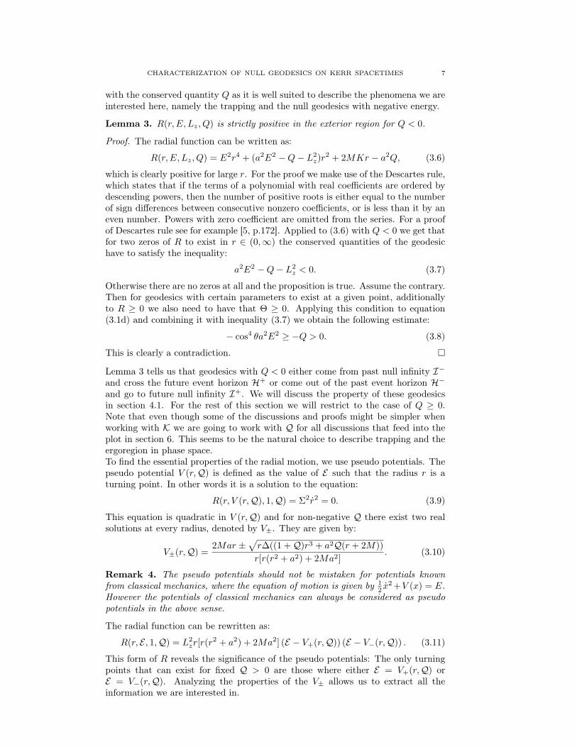
Lemma 3. R(r, E, Lz, Q) is strictly positive in the exterior region for Q < 0.

Proof. The radial function can be written as:

R(r, E, Lz, Q) = E2r4 + (a2E2 −Q− L2z)r

2 + 2MKr − a2Q, (3.6)

which is clearly positive for large r. For the proof we make use of the Descartes rule,which states that if the terms of a polynomial with real coefficients are ordered bydescending powers, then the number of positive roots is either equal to the numberof sign differences between consecutive nonzero coefficients, or is less than it by aneven number. Powers with zero coefficient are omitted from the series. For a proofof Descartes rule see for example [5, p.172]. Applied to (3.6) with Q < 0 we get thatfor two zeros of R to exist in r ∈ (0,∞) the conserved quantities of the geodesichave to satisfy the inequality:

a2E2 −Q− L2z < 0. (3.7)

Otherwise there are no zeros at all and the proposition is true. Assume the contrary.Then for geodesics with certain parameters to exist at a given point, additionallyto R ≥ 0 we also need to have that Θ ≥ 0. Applying this condition to equation(3.1d) and combining it with inequality (3.7) we obtain the following estimate:

− cos4 θa2E2 ≥ −Q > 0. (3.8)

This is clearly a contradiction.

Lemma 3 tells us that geodesics with Q < 0 either come from past null infinity I−and cross the future event horizon H+ or come out of the past event horizon H−and go to future null infinity I+. We will discuss the property of these geodesicsin section 4.1. For the rest of this section we will restrict to the case of Q ≥ 0.Note that even though some of the discussions and proofs might be simpler whenworking with K we are going to work with Q for all discussions that feed into theplot in section 6. This seems to be the natural choice to describe trapping and theergoregion in phase space.To find the essential properties of the radial motion, we use pseudo potentials. Thepseudo potential V (r,Q) is defined as the value of E such that the radius r is aturning point. In other words it is a solution to the equation:

R(r, V (r,Q), 1,Q) = Σ2r2 = 0. (3.9)

This equation is quadratic in V (r,Q) and for non-negative Q there exist two realsolutions at every radius, denoted by V±. They are given by:

V±(r,Q) =2Mar ±

√r∆((1 +Q)r3 + a2Q(r + 2M))

r[r(r2 + a2) + 2Ma2]. (3.10)

Remark 4. The pseudo potentials should not be mistaken for potentials knownfrom classical mechanics, where the equation of motion is given by 1

2 x2 +V (x) = E.

However the potentials of classical mechanics can always be considered as pseudopotentials in the above sense.

The radial function can be rewritten as:

R(r, E , 1,Q) = L2zr[r(r

2 + a2) + 2Ma2] (E − V+(r,Q)) (E − V−(r,Q)) . (3.11)

This form of R reveals the significance of the pseudo potentials: The only turningpoints that can exist for fixed Q > 0 are those where either E = V+(r,Q) orE = V−(r,Q). Analyzing the properties of the V± allows us to extract all theinformation we are interested in.


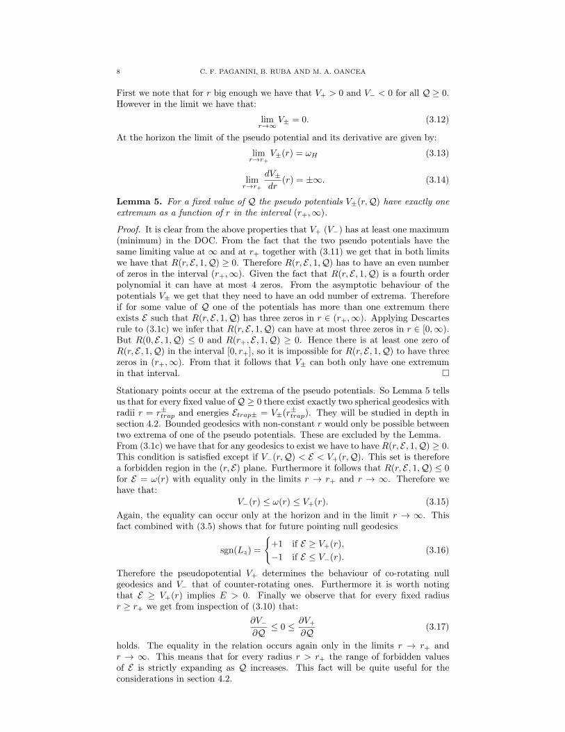
First we note that for r big enough we have that V+ > 0 and V− < 0 for all Q ≥ 0.However in the limit we have that:

limr→∞

V± = 0. (3.12)

At the horizon the limit of the pseudo potential and its derivative are given by:

limr→r+

V±(r) = ωH (3.13)

limr→r+

dV±dr

(r) = ±∞. (3.14)

Lemma 5. For a fixed value of Q the pseudo potentials V±(r,Q) have exactly oneextremum as a function of r in the interval (r+,∞).

Proof. It is clear from the above properties that V+ (V−) has at least one maximum(minimum) in the DOC. From the fact that the two pseudo potentials have thesame limiting value at ∞ and at r+ together with (3.11) we get that in both limitswe have that R(r, E , 1,Q) ≥ 0. Therefore R(r, E , 1,Q) has to have an even numberof zeros in the interval (r+,∞). Given the fact that R(r, E , 1,Q) is a fourth orderpolynomial it can have at most 4 zeros. From the asymptotic behaviour of thepotentials V± we get that they need to have an odd number of extrema. Thereforeif for some value of Q one of the potentials has more than one extremum thereexists E such that R(r, E , 1,Q) has three zeros in r ∈ (r+,∞). Applying Descartesrule to (3.1c) we infer that R(r, E , 1,Q) can have at most three zeros in r ∈ [0,∞).But R(0, E , 1,Q) ≤ 0 and R(r+, E , 1,Q) ≥ 0. Hence there is at least one zero ofR(r, E , 1,Q) in the interval [0, r+], so it is impossible for R(r, E , 1,Q) to have threezeros in (r+,∞). From that it follows that V± can both only have one extremumin that interval.

Stationary points occur at the extrema of the pseudo potentials. So Lemma 5 tellsus that for every fixed value ofQ ≥ 0 there exist exactly two spherical geodesics withradii r = r±trap and energies Etrap± = V±(r±trap). They will be studied in depth insection 4.2. Bounded geodesics with non-constant r would only be possible betweentwo extrema of one of the pseudo potentials. These are excluded by the Lemma.From (3.1c) we have that for any geodesics to exist we have to have R(r, E , 1,Q) ≥ 0.This condition is satisfied except if V−(r,Q) < E < V+(r,Q). This set is thereforea forbidden region in the (r, E) plane. Furthermore it follows that R(r, E , 1,Q) ≤ 0for E = ω(r) with equality only in the limits r → r+ and r → ∞. Therefore wehave that:

V−(r) ≤ ω(r) ≤ V+(r). (3.15)Again, the equality can occur only at the horizon and in the limit r → ∞. Thisfact combined with (3.5) shows that for future pointing null geodesics

sgn(Lz) =

+1 if E ≥ V+(r),

−1 if E ≤ V−(r).(3.16)

Therefore the pseudopotential V+ determines the behaviour of co-rotating nullgeodesics and V− that of counter-rotating ones. Furthermore it is worth notingthat E ≥ V+(r) implies E > 0. Finally we observe that for every fixed radiusr ≥ r+ we get from inspection of (3.10) that:

∂V−∂Q

≤ 0 ≤ ∂V+

∂Q(3.17)

holds. The equality in the relation occurs again only in the limits r → r+ andr → ∞. This means that for every radius r > r+ the range of forbidden valuesof E is strictly expanding as Q increases. This fact will be quite useful for theconsiderations in section 4.2.


Figure 1. This figure shows shapes of function ΘL2

zfor four choices

of values of conserved quotients.

3.2. The θ Equation. In Schwarzschild spacetimes, due to spherical symmetrythe motion of any geodesics is contained in a plane. This means that for everygeodesic there exists a spherical coordinate system in which it is constrained tothe equatorial plane θ = π

2 . This is no longer true in Kerr spacetimes, but mostgeodesics are still constrained in θ direction. The allowed range of θ is obtainedby solving the inequality Θ(θ,E, Lz, Q) ≥ 0. After multiplication with sin2(θ),Θ(θ, E, Lz, Q) can be expressed as a quadratic polynomial in the variable cos2(θ).Hence Θ(θ,E, Lz, Q) = 0 has two solutions given by:

cos2 θturn =a2E2 − L2

z −Q±√

(a2E2 − L2z −Q)2 + 4a2E2Q

2a2E2. (3.18)

For Q > 0 only the solution with the plus sign is relevant and the motion will alwaysbe contained in a band θmin < θeq < θmax symmetric about the equator θeq = π

2 .As |Lz| increases, this band shrinks. In fact only in the case Lz = 0 it is possiblefor a geodesic to reach the poles θ = 0, θ = π. Otherwise Θ(θ,E, Lz, Q) blows up to−∞ there. If Q < 0 both solutions are positive and the inclination of the geodesicwith respect to the equator is also constrained away from the equator, so eitherθeq < θmin < θmax or θeq > θmax > θmin . These trajectories will be containedin a disjoint band which intersects neither the equator nor the pole. This bandcan degenerate to a point, i.e. there exist null geodesics which stay at θ = const.The relevance of these trajectories and how they are connected to the Schwarzschildcase will be discussed in the next section. All possibilities for the potentials thatconstrain the motion in θ direction are summarized in the Figure 1.

4. Special Geodesics

We will now apply the discussions of the last section to describe a number ofspecial geodesics in Kerr geometries. All of these are in some way related to eitherthe black hole stability problem or the black hole uniqueness problem.

4.1. Radially In-/Out-going Null Geodesics. In this section we find geodesicswhich generalize the radially ingoing and outgoing congruences in Schwarzschildspacetimes. In section 3.1 we saw that the geodesics with Q < 0 extend from thehorizon to infinity. In section 3.2 we saw that Q < 0 is again a special case, as thesenull geodesics can never intersect the equator and in the extreme case are evenconstrained to a fixed value of θ. At first this behaviour seems odd, but a similarsituation can be observed in Schwarzschild. If we look at geodesics which move in aplane with inclination θ0 about the equatorial plane we see that there exists a set of


null geodesics with similar properties as the ones with Q < 0 in Kerr. It is clear thatthe radially ingoing geodesic which moves orthogonally to the axis around which theplane of motion was rotated, moves at fixed θ value, namely that at which the planeis inclined with respect to the equatorial plane, hence θ = π/2 ± θ0. Furthermoresome null geodesics reach the horizon before intersecting the equatorial plane. Theydon’t necessarily move at fixed θ but their motion in θ direction is still constrainedaway form the equatorial plane and away from the poles of the coordinate system.Now we want to investigate the null geodesics which move at fixed θ in Kerr. De-manding that θ = const. is equivalent to requiring Θ = d

dθΘ = 0. From theseconditions we obtain:

Lz = ±aE sin2 θ, (4.1a)

Q = −a2E2 cos4 θ, (4.1b)K = 0. (4.1c)

By choosing the plus sign for Lz in the above equation, it follows from the remainingequations of motion that:

φ

t=dφ

dt= ω(r), (4.2a)

r

t=dr

dt= ± ∆

r2 + a2. (4.2b)

This congruence is generated by the principal null directions e0 ± e1. When choos-ing the minus sign for Lz in (4.1) the remaining equations of motions can not besimplified in a similar manner. In the case a = 0 these are the radially in-/outgoingnull geodesics. An interesting observation is that along these geodesics the innerproduct of the (∂t)

µ vector field is monotone. A simple calculation shows that:

γµ∇µ((∂t)ν(∂t)ν) = r

2M(r2 − a2 cos2 θ)

Σ2+ θ

2Ma2r sin 2θ

Σ2. (4.3)

For the principal null congruence we have θ = 0, the coefficient of r is positive andthere is no turning point in r. This property might be interesting in the context ofthe black hole uniqueness problem. If one could show a similar monotonicity state-ment for a congruence of null geodesics in general stationary black hole spacetimes,one could conclude that the ergosphere in such spacetimes has only one connectedcomponent enclosing the horizon. This is a necessary condition if one wants to showthat no trapped T-orthogonal null geodesics can exist in that case.

4.2. The Trapped Set. One of the most important features of geodesic motionin black hole spacetimes is the possibility of trapping. A geodesic is called trappedif its motion is bounded in a spatially compact region away from the horizon. InKerr this corresponds to the geodesics motion being bounded in r direction. Thisis only possible if r = const. or if the motion is between two turning points ofthe radial motion. For null geodesics in Kerr we ruled out the second option inLemma 5. We will now discuss orbits of constant radius.4 These null geodesicsare stationary points of the radial motion, hence null geodesics with r = r = 0.Dividing equation (3.1c) by Σ and taking the derivative with respect to λ we seethat this condition is equivalent to R(r) = d

drR(r) = 0. The solutions to theseequations can be parametrized explicitly by, cf. [19]:

Etrap(r) = −a(r −M)

A(r)= ω(r)

(1− 2r∆

A(r)

)(4.4)

4Null geodesics of constant radius are often referred to as "spherical null geodesics" but it isimportant to note that r = const. does not imply that the whole sphere is accessible for suchgeodesics.


Figure 2. Plot of the relation between the radius of the equatorialtrapped null geodesics at r1 and r2, the trapped null geodesic withLz = 0 at r3 and the horizon at r+ for all values of a.

Qtrap(r) = − B(r)

A2(r)(4.5)

A(r) = r3 − 3Mr2 + a2r + a2M = (r − r3)P2(r) (4.6)B(r) = r3(r3 − 6Mr2 + 9M2r − 4a2M) = (r − r1)(r − r2)P4(r) (4.7)

where P2 and P4 are polynomials in r, quadratic and quartic respectively, which arestrictly positive in the DOC. The following three radii are particularly important:

r1 = 2M

(1 + cos

(2

3arccos

(− a

M

)))(4.8)

r2 = 2M

(1 + cos

(2

3arccos

( aM

)))(4.9)

r3 = M + 2

√M2 − a2

3cos

(1

3arccos

(M(M2 − a2)

(M2 − a2

3 )32

))(4.10)

satisfying the inequalities:

M < r+ < r1 < r3 < r2 < 4M (4.11)

for a ∈ (0,M). Orbits of constant radius are allowed only inside the interval [r1, r2],because outside of it Q would have to be negative. This possibility has alreadybeen excluded in Lemma 3. The boundaries of the interval at r = r1 and r = r2

correspond to circular geodesics constrained to the equatorial plane with Q = 0.The trapped null geodesics at r = r3 have Lz = 0 which is the reason why thefunctions Etrap and Qtrap blow up there. From the second representation in (4.4)we see that Etrap(r)− ω(r) is positive in [r1, r3) and negative in (r3, r2]. Combinedwith (3.16) this implies that the stationary points in [r1, r3) correspond to extremaof V+ and the stationary points in (r3, r2] correspond to extrema of V−. In Lemma5 we showed that V+ and V− both have exactly one extremum. Since extrema ofthe pseudo potentials always correspond to orbits of constant radius, we get thatthe extrema of V+(r,Q) and V−(r,Q) have to be within the intervals [r1, r3) and(r3, r2] respectively for any value of Q. In Figure 2 we plot the behaviour of theseintervals as a function of a/M .


We now know that the maps given by:

[0,∞) 3 Q 7→ r+trap ∈ [r1, r3)

[0,∞) 3 Q 7→ r−trap ∈ (r3, r2]

which take Q into radii of trapped geodesics corresponding to the unique maximumof V+(r,Q) and minimum of V−(r,Q) respectively are one-to-one and thereforemonotone. By using (4.5) the sign of their derivatives can be easily evaluated insome ε-neighbourhood of r = r3 where the term of highest order in 1

r−r3 dominates:

∂r−trap∂Q

< 0 <∂r+trap

∂Q. (4.12)

By the equation (3.17) and the fact that radii of trapping always correspond toglobal extrema of the pseudo potentials we get that:

∂

∂QEtrap(r−trap(Q)) < 0 <

∂

∂QEtrap(r+

trap(Q)). (4.13)

Using the chain rule and combining these two facts we obtain:∂Etrap∂r

> 0. (4.14)

These inequalities provide an important piece of the picture of the influence of Qon the trapped geodesics. We have Q = 0 for the outermost circular geodesics andas we increase it, the radii of trapping converge towards r = r3 while E blows upto ±∞, with the sign depending on the direction from which we approach r3. Wecan also desciribe the function Etrap(r): it starts with some finite positive value atr = r1 and increases monotonically to +∞ as r approaches r3. There it jumps to−∞ and increases again to a finite negative value at r = r2.It is interesting to ask what region in physical space is accessible for trappedgeodesics. By plugging (4.5) and (4.4) into the equation Θ = 0 we get that fora geodesic with r = const.:

cos2 θturn =2√Mr2∆(2r3 − 3Mr2 + a2M)− r(r3 − 3M2r + 2a2M)

a2(r −M)2(4.15)

holds. This gives two turning points in θ direction which are symmetric about theequatorial plane. The whole region of trapping in the (r, θ) plane is bounded bycurves defined implicitly by (4.15) and r1 ≤ r ≤ r2. Figure (3) presents this set fora particular value of a.

Remark 6. Two warnings:(1) One has to be careful when interpreting Figure 3 (and the plots in the Mathe-

matica notebook). Despite the fact that the region in physical space occupiesfinite range of r values, every individual trapped null geodesic is still con-strained to a fixed radius. For an insight on what those trajectories look likein detail we recommend the study of [19].

(2) When taking a → M in the Mathematica notebook the ergosphere appearsto develop a kink on the rotation axis. This is an artifact of the coordi-nate system, as the ergosphere coincides with the horizon there and is thusorthogonal to itself.

4.3. T-Orthogonal Null Geodesics. In the ergoregion there exist null geodesicswith negative values of E. In physical space they are constrained to the regiondefined by equation (2.20). From Lemma 3 we know that geodesics with Q < 0reach either I+ or come from I− and can therefore not have negative values of E.This allows us to use the pseudo potentials to give a more precise characterizationof the ergoregion in phase space. It is located in the region where V−(Q) > 0,


Figure 3. The region accessible for trapped null geodesics for a =0.902. The shaded region represents the black hole, r ≤ r+. Theonly qualitative change in this picture occurs at a = 1√

2because

at this value the region of trapping starts intersecting with theergoregion.

between E = 0 and V−(Q). An immediate consequence of that is, that all futurepointing null geodesics with negative E begin at the past event horizon and end atthe future event horizon. Furthermore they must have Lz < 0. Those null geodesicswith E = 0 can reach the boundary of the ergoregion. In this case equation (3.1d)gives us, that:

Q =cos2(θmax)

sin2(θmax). (4.16)

When calculating the turning points from equation (3.1c) we get that:

sin2(θmax)R

(r, 0, 1,

cos2(θmax)

sin2(θmax)

)= −r2 + 2Mr − a2cos2(θmax) = 0. (4.17)

The only solution to this equation in the exterior region is:

rturn(θmax) = M +√M2 − a2cos2(θmax) (4.18)

which is exactly the location of the ergo sphere (2.20). So V−(Q) > 0 can be consid-ered as the boundary of the ergoregion in phase space. From this considerations wesee immediately that T-orthogonal null geodesics are clearly non-trapped in Kerr.In fact there do not even exist any trapped null geodesics orthogonal to:

Kν = (∂t)ν + εmin(∂φ)ν (4.19)

where εmin = min[|V+(0, r1)|, |V−(0, r2)|].

5. Trapping as a Set of Directions

In this section we will link the previous discussion to the black hole shadows.We introduce a more formal framework for the discussion. This allows us to give amore technical discussion of the trapped sets in Schwarzschild and Kerr black holes.


5.1. Framework. First we have to introduce the basic framework and notations.Let M be a smooth manifold with Lorenzian metric g. At any point p in M youcan find an orthonormal basis (e0, e1, e2, e3) for the tangent space, with e0 beingthe timelike direction. It is sufficient to treat only future directed null geodesics asthe past directed ones are identical up to a sign flip in the parametrization. Thetangent vector to any future pointing null geodesic can be written as:

γ(k|p)|p = α(e0 + k1e1 + k2e2 + k3e3) (5.1)

where α = −g(γ, e0) and k = (k1, k2, k3) satisfies |k|2 = 1, hence k ∈ S2. Thegeodesic is independent of the scaling of the tangent vector as this corresponds toan affine reparametrization for the null geodesic. We will therefore set α = 1 in thefollowing discussion. The S2 is often referred to as the celestial sphere of a timelikeobserver at p whose tangent vector is given by e0, cf. [16, p.8].For the further discussions we fix the tetrads. We can make the following definition:

Definition 7. Let γ(k|p) denote a null geodesic through p for which the tangentvector at p is given by equation (5.1).

It is clear that γ(ka|p) and γ(kb|p) are equivalent up to parametrization if ka = kb.Suppose now thatM is the exterior region of a black hole spacetime with completefuture and past null infinity I± and a boundary given by the future and past eventhorizon H+ ∪H−. We can then define the following sets on S2 at every point p.

Definition 8. The future infalling set: ΩH+(p) := k ∈ S2|γ(k|p) ∩H+ 6= ∅.The future escaping set: ΩI+(p) := k ∈ S2|γ(k|p) ∩ I+ 6= ∅ .The future trapped set: T+(p) := k ∈ S2|γ(k|p) ∩ (H+ ∪ I+) = ∅.The past infalling set: ΩH−(p) := k ∈ S2|γ(k|p) ∩H− 6= ∅.The past escaping set: ΩI−(p) := k ∈ S2|γ(k|p) ∩ I− 6= ∅.The past trapped set: T−(p) := k ∈ S2|γ(k|p) ∩ (H− ∪ I−) = ∅

We finish the section by defining the trapped set to be:

Definition 9. The trapped set: T(p) := T+(p) ∩ T−(p).

The region of trapping in the manifoldM is then given by:

Definition 10. Region of trapping: A := p ∈M|T(p) 6= ∅.

5.2. The trapped sets in Schwarzschild. The discussion of Schwarzschild servesas an easy example for the various concepts.

Definition 11. We refer to the set ΩH−(p)∪T−(p) as the shadow of the black hole.

However for any practical purposes information about its boundary which is given byT−(p) is good enough. An observer in the exterior region can only observe light frombackground sources along directions in the set ΩI−(p). From the radial equationwe get immediately that if k = (k1, k2, k3) ∈ T+(p) then k = (−k1, k2, k3) ∈ T−(p).Hence the properties of the past and the future sets are equivalent. This is trueboth in Schwarzschild and Kerr.An explicit formula for the shadow of a Schwarzschild black hole was first given in[18]. In Schwarzschild the orthonormal tetrad (2.6) reduces to:

e0 =1√

1− 2M/r∂t, e1 =

√1− 2M/r∂r, (5.2)

e2 =1

r∂θ, e3 =

1

r sin θ∂φ.

To determine the structure of T±(p) in Schwarzschild it is sufficient to considerp in the equatorial plane and k = (cos Ψ, 0, sin Ψ) with Ψ ∈ [0, π]. The entiresets T±(p) are then obtained by rotating around the e1 direction. Note that from


(a) (b) (c)

Figure 4. The trapped set on the celestial sphere of a standardobserver at different radial location in a Schwarzschild DOC. Ob-server (a) is located outside the photon sphere at r = 3.9M , ob-server (b) is located on the photon sphere at r = 3M and finallyobserver(c) is located between the horizon and the photonsphere atr = 2.5M . One can see that the future trapped set moves from theingoing hemisphere in (a) to the outgoing hemisphere in (c) as onevaries the location of the observer. The future and past trappedset coincide on the r = 0 line when the observer is located on thephoton sphere at r = 3M in (b)

the tetrad it is obvious that E(k) = E(r) is independent of Ψ. On the otherhand Lz(k) is zero for Ψ = 0, π and maximal for Ψ = π/2. Away from thatmaximum, Lz is a monotone function of Ψ. Note that the geodesic that correspondsto Ψ = π/2 has k1 = 0 and thus a radial turning point. Thus the E/Lz valueof this geodesic corresponds to the minimum value any geodesic can have at thispoint in the manifold. For r 6= 3M this is smaller then the value of trappingand thus there exist two k with the property that E/Lz(k) = 1/

√27M2. One of

them has k1 > 0 and therefore r > 0 and one has r < 0. For r > 3M the firstcorresponds to T−(p) and the second corresponds to T+(p). For 2M < r < 3Mthe roles are reversed. For r = 3M we have T+(p) = T−(p) = (0, k2, k3). InFigure 4 we depict these three cases for some fixed radii. To conclude we see thatT+(p) and T−(p) are circles on the celestial sphere independent of the value of r(p).In [16, p.14] it is shown that Lorentz transformations on the observer correspondto conformal transformations on the celestial sphere. They are equivalent up toMöbius transformations on the complex plane when considering the S2 to be theRiemann sphere. Hence circles on the celestial sphere stay circles under Lorentztransformations. As a consequence if r(pa) 6= r(pb) then there exists a Lorentztransformation (LT) such that T−(pa) = LT[T−(pb)]. This concept is sufficientlyimportant that it deserves a proper definition.

Definition 12. The shadows at two points p1, p2 are called degenerate if, uponidentification of the two celestial spheres by the orthonormal basis, there exists anelement of the conformal group on S2 that transforms T−(p1) into T−(p2).

Remark 13. The shadow at two points p1, p2 being degenerate implies that forevery observer at p1 there exists an observer at p2 for which the shadow on S2 isidentical. Because this notion compares structures on S2, the two points do nothave to be in the same manifold for their shadows to be degenerate. Just from theshadow alone an observer can not distinguish between these two configurations.

The only reliably information an observer can obtain is thus, that T−(p) is aproper circle on his celestial sphere.

5.3. The trapped sets in Kerr. We will now discuss the properties of the setsT±(p) in Kerr. Note that the equations of motion for r (3.1c) and θ (3.1d) have twosolutions that differ only by a sign for a fixed combination of E,Lz,K. Therefore


we know that the trapped sets will have a reflection symmetry across the k1 = 0and the k2 = 0 planes. A sign change in k2 maps both sets T±(p) to themselves,while a sign flip in k1 maps T+(p) to T−(p) and vice versa.In the following we will use the parametrization of [10]. We introduce the coordi-nates ρ ∈ [0, π] and ψ ∈ [0, 2π) on the celestial sphere. Thus (5.1) can be writtenas:

γ(ρ, ψ)|p = α(e0 + cos(ρ)e1 + sin(ρ) cos(ψ)e2 + sin(ρ) sin(ψ)e3) (5.3)The direction towards the black hole is given by ρ = π. Following [10] one finds thefollowing parametrization of the celestial sphere in terms of constants of motion:

sin(ψ) =(L − a) + a cos2(θ)√

K sin(θ)

∣∣∣∣p

, (5.4a)

sin(ρ) =

√∆K

r2 − a(L − a)

∣∣∣∣∣p

, (5.4b)

Analog to the functions (4.4) and (4.5) which give the value of the conserved quan-tities in terms of the radius of trapping, we can give such relations for the conservedquotientsK and L in this formulation they can be found for example in [10]. To differbetween the trapped radius and the observers radius we use x ∈ [rmin(θ), rmax(θ)] toparametrize the conserved quantities of the trapped set. Here rmin(θ) and rmax(θ)are given as the intersection of a cone of constant θ with the boundary of the area oftrapping. Note that it is part of the following proof to show that the given intervalis in fact the correct domain for the parameter x. The parameter x here corre-sponds to the radius of the trapped null geodesic which a particular future trappeddirection is asymptoting to. We have then:

K =16x2∆(x)

(∆′(x))2(5.5a)

a(L − a) =

(x2 − 4x∆(x)

∆′(x)

)(5.5b)

where ∆′(x) = 2x−2M is the partial derivative of ∆(x) with respect to x .Plugging(5.5) into (5.4) we obtain:

sin(ψ) =∆′(x)x2 + a2 cos2(θ(p)) − 4x∆(x)

4x√

∆(x)a sin(θ(p))(5.6a)

sin(ρ) =4x√

∆(r(p))∆(x)

∆′(x)(r(p)2 − x2) + 4x∆(x):= h(x) (5.6b)

We are now ready to prove the following Theorem.

Theorem 14. The sets T+(p) and T−(p) are smooth curves on the celestial sphereof any timelike observer at any point in the exterior region of any subextremal Kerrspacetime.

Proof. We start by anayzing the right hand side of (5.6a):

d

dx

(∆′(x)x2 + a2 cos2(θ(p)) − 4x∆(x)

4x√

∆(x)a sin(θ(p))

)

=x2 + a2 cos2(θ(p))((M − x)3 −M(M2 − a2))

2x2∆(x)3/2a sin(θ(p)),

(5.7)

which is strictly negative for x ∈ (r+,∞). The limit of the right hand side of (5.6a)is given by ∞ for x → r+ and −∞ for x → ∞. Therefore the right hand side isinvertible and x(sin(ψ)) is a smooth function of ψ with extrema at the extremalpoints of sin(ψ). As was shown in [10] the minimum xmin(θ(p)) at ψ = π/2 andthe maximum of xmax(θ(p)) at ψ = 3π/2 correspond exactly to the intersections


of a cone with constant θ with the boundary of the region of trapping. This canbe seen by setting the left hand side of (5.6a) equal to ±1, taking the square ofthe equation, solving for cos2(θ) and comparing to (4.15). Important here is that[xmin(θ(p)), xmax(θ(p))] ⊂ [r1, r2] for all values of θ(p). Now we take a look at theright hand side of equation (5.6b):

d

dx(h(x)) =

8(r(p)2 − x2)∆(r(p))((x−M)3 +M(M2 − a2))√∆(r(p))∆(x)(4x∆(x) + (r(p)2 − x2)∆′(x))2

. (5.8)

This is positive when x < r(p) and negative when x > r(p). The denominator nevervanishes for x ∈ (r+,∞) because:

(4x∆(x) + (r(p)2 − x2)∆′(x))|r(p)=r+,x=r+ = 0 (5.9)

andd

dx(4x∆(x) + (r(p)2 − x2)∆′(x)) = 2(3x2 − 6Mx+ 2a2 + r(p)2) > 0 (5.10)

d

dr(p)(4x∆(x) + (r(p)2 − x2)∆′(x)) = 2r(p)∆′(x) > 0, (5.11)

where we used r(p) > r+ > M > a in (5.10).If we set x = r(p) in (5.6b) then the right hand side is equal to 1. Furthermore inany of the limits r(p)→ r+, r(p)→∞, x→ r+, and x→∞ it goes to zero.

Case 1. If p /∈ A hence if r(p) /∈ [xmin(θ(p)), xmax(θ(p))] then the two functions:

ρ1(ψ) = arcsin(h(x(ψ))) : [0, 2π)→ [ρ1min, ρ1max

] ⊂(

0,π

2

)(5.12)

ρ2(ψ) = π − arcsin(h(x(ψ))) : [0, 2π)→ [ρ2min, ρ2max

] ⊂(π

2, π)

(5.13)

are both smooth with ρ1(0) = ρ1(2π) and ρ2(0) = ρ2(2π). If p is between the regionof trapping and the asymptotically flat end, the function ρ2(ψ) corresponds to T+(p)and ρ1(ψ) corresponds to T−(p). Because (π/2, π] corresponds to the geodesic withr < 0. If p is between the region of trapping and the horizon then the role of ρ1(ψ)and ρ2(ψ) are switched.

Case 2. If p ∈ A we need to do some extra work. For simplicity we only considerthe interval ψ ∈ [π/2, 3π/2] as the rest follows by symmetry of sin(ψ) in [0, π] acrossπ/2 and in [π, 2π] across 3π/2. Let arcsin(x) map into this interval, then we define:

ψ0(r(p)) = arcsin

(∆′(r(p))r(p)2 + a2 cos2(θ(p)) − 4r(p)∆(r(p))

4r(p)√

∆(r(p))a sin(θ(p))

). (5.14)

The two functions:

ρ3(ψ) =

arcsin(h(x(ψ))) if ψ ∈ [π/2, ψ0(r(p))]

π − arcsin(h(x(ψ))) if ψ ∈ (ψ0(r(p)), 3π/2](5.15)

ρ4(ψ) =

π − arcsin(h(x(ψ))) if ψ ∈ [π/2, ψ0(r(p))]

arcsin(h(x(ψ))) if ψ ∈ (ψ0(r(p)), 3π/2](5.16)

are then smooth on [π/2, 3π/2]. For a proof see Appendix A and note that at ψ0,h(x(ψ)) satisfies the conditions required in the appendix. Since p ∈ A we have thatxmin(θ(p)) < r(p) < xmax(θ(p)). Therefore the geodesic on the celestial sphereparametrized by xmax(θ(p)) has to have r > 0 and thus has to be in [0, π/2). Onthe other hand the geodesic on the celestial sphere parametrized by xmin(θ(p)) hasto have r < 0 and thus has to be in (π/2, π]. In fact by the monotonicity of the righthand side of (5.6a) and the fact that x(ψ0) = r(p) we know that for ψ ∈ [π/2, ψ0)we have x(ψ) < r(p) and for ψ ∈ (ψ0, 3π/2] we have x(ψ) > r(p). Thus we canconclude that for p ∈ A, ρ4 corresponds to T+(p) and ρ3 corresponds to T−(p) andthus both sets are smooth.


Case 3. In the special case when r(p) = xmax(θ(p)) or r(p) = xmin(θ(p)) thefunctions ρ1 and ρ2 describing T±(p) do reach ρ = π/2 at ψ = 3π/2 or ψ = π/2respectively. However since in these cases we have that:

d2

dψ2(h(x(ψ))) = 0, (5.17)

the two sets meet at this point tangentially and do not cross over into the otherhemisphere.

This concludes the proof.

Remark 15. In [10] it was observed that ρmax of T+(p) always corresponds tothe trapped geodesic with xmin(θ(p)) and ρmin of T+(p) always corresponds tothe trapped geodesic with xmax(θ(p)) . When p is outside the region of trappingh(x)|xmax

is a local maximum of h(x(ψ)) (as a function of ψ) and h(x)|xminis a

local minimum of h(x(ψ)). When p is between the region of trapping and the hori-zon h(x)|xmax is a local minimum of h(x(ψ)) and h(x)|xmin is a local maximumof h(x(ψ)). Since outside T+(p) is always described by ρ2(ψ) and inside by ρ1(ψ),ρmin then always corresponds to xmin and ρmax always corresponds to xmax. Thisalso holds for p ∈ A.This observation means that the null geodesic approaching the innermost photonorbit has the smallest impact parameter (deviation from the radially ingoing null ge-odesic) and the null geodesic approaching the outermost photon orbit has the largestimpact parameter.For T−(p) the correspondence is switched.

Remark 16. The parametrization for sin(ψ) breaks down on the rotation axis, theone for sin(ρ) however remains valid with only one possible value for x = r3. Dueto the symmetry at these points we know that T±(p) are described by proper circleson the celestial sphere. The PND is aligned with the axis of the rotation symmetryand hence the sets are symmetric under rotation along ψ. The situation is thereforeequivalent to Schwarzschild and an observer can not distinguish whether he observesa Schwarzschild black hole or a Kerr black hole in the direction of the rotation axis.

Remark 17. We have only proved Theorem 14 for one standard observer at anyparticular point. However since any other observer at this point is related to thestandard observer by a Lorentz transformation and the Lorentz transformations actas conformal transformations on the celestial sphere [16, p.14], the Theorem indeedholds for any observer. In [9] the quantitative effect on the shape of the shadow ofboosts in different directions are discussed.

Remark 18. The parametrization for the trapped set on the celestial sphere of anystandard observer in [10, 11] was derived for a much more general class of space-times. Therefore Theorem 14 might actually hold for these cases as well. Howeverthis is beyond the scope of this paper.

From Theorem 14 we immediately get the following Corollary:

Corollary 19. For any observer at any point p in the exterior region of a subex-tremal Kerr spacetime we have that for any k ∈ T+(p) and any ε > 0

• Bε(k) ∩ ΩH+(p) 6= ∅• Bε(k) ∩ ΩI+(p) 6= ∅.

So if we interpret the celestial sphere as initial data space for null geodesics startingat p, the Corollary is a coordinate independent formulation of the fact that trappingin the exterior region of subextremal Kerr black holes is unstable.See Figure 5 as an example on how the trapped sets change under a variation ofthe radial location of the observer.


(a) (b) (c)

(d) (e)

Figure 5. The trapped set on the celestial sphere of a standardobserver at different radial locations in the equatorial plane of theexterior region of a Kerr black hole with a = 0.9. Observer (a)is located outside the region of trapping at r = 5M . Observer(b) is located on the outer boundary of the region of trapping atr = r2 = 3.535M . Observer (c) is located inside the region oftrapping at r = r3 = 2.56M . Observer (d) is located on the innerboundary of the area of trapping at r = r1 = 1.73M Finally ob-server (e) is located between the horizon and the area of trappingat r = 1.59M . Again one can observe how the two trapped setsmove in opposite directions on the celestial sphere as the observerapproaches the black hole. In (a) the future trapped set is on theingoing hemisphere and the past trapped set is on the outgoinghemispere. In (b) they meet in one point tangentially but are stillentirely in one hemisphere except for that one point. In (a) thetrapped sets intersect in two points and both have parts in bothhemispheres. In (d) they only meet at one point tangentially again(now on the "other" side of the celestial sphere) and finally in (e)the future trapped set is entirely in the outgoing hemisphere andthe past trapped set is entirely in the ingoing hemisphere.

Even though the qualitative features of T±(p) do not change under a change ofparameters, the quantitative features do. In [13, 14] it is discussed what informationcan be read of from the shadow at infinity. For points inside the manifold asconsidered in this work, it is unclear to the authors what the maximal amountof information is that an observer can obtain from the shape of the shadow. Inthe following we will present numerical calculations that suggest that the radialdegeneracy of the shadow is broken in Kerr spacetimes away from the symmetryaxis. We take the stereographic projection: [16, p.10]

ζ =x+ iy

1− z(5.18a)

x = sin(ρ) sin(ψ) y = sin(ρ) cos(ψ) z = cos(ρ) (5.18b)

of T−(p) in order to compare the exact shape of the shadow for different observers.Here the values of ρ and ψ are given by the parametrization in (5.5). The aboveprojection for the celestial sphere of a standard observer in the exterior region of


a Kerr black hole guarantees that projection of the shadow in the complex planewill have a reflection symmetry about the real axis. This is due to the symmetryof the shadow on the celestial sphere of a standard observer under a sign flip in thek2 component. To compare conformal class of the shadow for observers in differentpoints of different black hole spacetimes we establish the notion of a canonicalobserver together with a canonical projection. This will allow us to compare theshape of the shadow for these observers directly. The canonical observer togetherwith the canonical projection are defined in such a way that the points on T−(p) withΨ = π/2, 3π/2 will correspond to the points (1, 0) and (−1, 0) in the complex plane.On the practical side we take the stereographic projection along the radially ingoingdirection for the standard observer and then apply conformal transformations to theprojection of the shadow (translation and rescaling). In the following CS2 denotesthe union of all conformal transformations on S2.

Remark 20. In order to prove that the conformal class of two curves x and yon S2 are equal it is sufficient to find an x0 ∈ CS2 [x] and a y0 ∈ CS2 [y] suchthat x0 = y0. By choosing a canonical observer, we choose a fix representativec0[p] ∈ CS2 [T−(p)] of each conformal class and thereby eliminate the freedom ofperforming conformal transformations on the celestial sphere of an observer. Henceif the shape of the canonical representative of any two shadows c0[p1(a1, θ1, r1)],c0[p2(a2, θ2, r2)] coincide, then their conformal class is equal. On the other hand ifc0[p1(a1, θ1, r1)] 6= c0[p2(a2, θ2, r2)] then the conformal classes of the shadow at p1

and that at p2 are different.

Note that when investigating for degeneracies numerically only negative answersare reliable, because an apparent degeneracy could simply be due to the fact thatthe difference between the shadows of two canonical observers is below the scale ofthe numerical resolution. The apparent breaking of the radial degeneracy in Kerrspacetimes can be seen in Figure 6, where we plotted two black hole shadows, forcanonical observers located in a Kerr spacetime with a = 0.99, at θ = π/2, anddifferent r values: r1 = 5, r2 = 50. These particular values were chosen becausefor this case the degeneracy breaking is visible by the naked eye from the plotin Figure 6. In general the breaking of the radial degeneracy is hardly visible inthe plot. Establishing a rigorous proof for the breaking of the radial degeneracy,as well as investigation the possibility for the shadow to have some complicateddegeneracy of the form f(a, r, θ) = const., where f is function of these parameters,is subject for further investigations. The breaking of the radial degeneracy impliesthat in principle when observing the shadow of a black hole, as intended by theEvent Horizon Telescope, one would have to take the distance from said blackhole into consideration when trying to extract the black holes parameters from theobservation. However the influence of the radial degeneracy for far away observersis quite likely a lot smaller than the resolution that can be achieved from suchobservations.


Figure 6. Breaking of the radial degeneracy for the shadow of aKerr black hole. Two canonical observers with a = 0.99, at θ = π/2,for two different values r = 5 and r = 50.

6. Application

Everything we have derived about the behaviour of null geodesics in Kerr space-times can be represented in a couple of simple plots. See Figure 7, Figure 4 andFigure 5 as examples; in the Mathematica notebook provided with this paper [1]the parameters a/M and Q as well as the location of the observer r(p), θ(p) canbe varied. This allows one to develop an intuitive understanding of the influence ofthese parameters.Furthermore by the eikonal approximation it is clear, that a massless wave equationshould relate to the null geodesic equation in the limit of high frequencies. In [7] itis shown that when separating the wave equation Σψ = 0 the ODE for the radialfunction in Schrödinger form can be written as:

d2u

dr∗ 2+

(R(r, E = ω,Lz = m,L2 = λlm)

(r2 + a2)2− F (r)

)u = 0 (6.1)

with F (r) = ∆r2+a2 (a2∆ + 2Mr(r2 − a2)) ≥ 0 and hence we have the following

relations:ω ∼ E, m ∼ Lz, λlm ∼ L2. (6.2)

When trying to understand the different treatments of different parameter rangesin [7] it is helpful to play with the parameters of the pseudo potential in the Math-ematica notebook provided with this paper [1]. The construction of the differentmode currents becomes much more intuitive when thinking about where in Figure7 the corresponding parameters are located. Note that in the high frequency limitthe pseudo potentials correspond to the location of ω2−V (r, ω,m,Λ) = 0 and hence


Figure 7. Plot of the pseudo potentials V± as function of a com-pactified radial coordinate in the exterior region for a = 0.764 andQ = 0.18. Its qualitative features are preserved when a and Q arechanged. The location of trapping in phase space is indicated bythe function Etrap(r). The extrema of the pseudo potentials arethe intersection of V+ and V− with this function. Therefore theyslide on this curve as Q increases. The area filled in gray corre-sponds to geodesics with E < 0. It is clear from this plot thatthe regions occupied by geodesics of negative energy and trappedgeodesics respectively are disjoint in phase space.

the location where the leading contribution to the bulk terms of the Qy and Qh

currents change their sign.Another interesting observation is that combining the results in section 4.2 and sec-tion 4.3 we can see that to separate trapping from the ergoregion in physical spaceit is sufficient if we restrict the null geodesics to be either co- or counter-rotating.In the co-rotating case there simply does not exist an ergoregion and the statementis clear. In the counter rotating case trapping is constrained to r ∈ (r3, r2] andr3 > 2M ≥ rergo for all Kerr spacetimes with a < M . In this direction particu-larly interesting might be the potential functions Ψ± in [12] which have interestingproperties in physical space.

Acknowledgements. We are grateful to Lars Andersson, Volker Perlick and SiyuanMa for helpful discussions and their comments on the manuscript.

Appendix A.

Let f(x) be a smooth function on [−1, 1] vanishing at the boundary points witha unique maximum with value 1 at zero. Hence f(0) = 1, f ′(0) = 0 and f ′′(0) < 0.We then define:

g1a(x) = arcsin(f(x)) : [−1, 0)→[0, π/2) (A.1)g2a(x) = π − arcsin(f(x)) : [−1, 0)→(π/2, π] (A.2)g1b(x) = arcsin(f(x)) : (0, 1]→[0, π/2) (A.3)g2b(x) = π − arcsin(f(x)) : (0, 1]→(π/2, π] (A.4)


Note that g′1a/b(x) = −g′2a/b(x). We then calculate:

d

dxg1a(x) =

f ′(x)√1− f(x)2

. (A.5)

Note that both the nominator and denominator vanish as x goes to zero. Howeverto apply the rule of l’Hopital we have to consider the square of the expression. Wethen get:

limx→0

(d

dxarcsin(f(x))

)2

= limx→0

−f ′′(x)

f(x)= −f ′′(0). (A.6)

Thus d/dx(arcsin(f(x)))|x=0 =√−f ′′(0). The sign is chosen based on the fact that

d/dx(arcsin(f(x))) > 0 for x ∈ [1, 0) . Note that on [−1, 0) the derivative of g1(x)is positive while on (0, 1] it is negative. Together this gives us that the function:

g(x) =

g1a(x) if x ∈ [−1, 0)

π/2 if x = 0

g2b(x) if x ∈ (0, 1]

(A.7)

is smooth at x = 0 and therefore on [−1, 1] with d/dx(g(x))|x=0 =√−f ′′(0).

References

1. http://www.aei.mpg.de/KerrNullgeodesicsPlots, (Direct URL to download of notebook).2. J.M. Bardeen, Black Holes 215-39, CRC Press, January 1973 (en).3. Brandon Carter, Global Structure of the Kerr Family of Gravitational Fields, Physical Review

174 (1968), no. 5, 1559–1571.4. S. Chandrasekhar, The mathematical theory of black holes, Oxford Classic Texts in the Phys-

ical Sciences, The Clarendon Press, Oxford University Press, New York, 1998, Reprint of the1992 edition. MR 1647491

5. P. M. Cohn, Algebra. Volume 1. Second Edition, 2nd edition ed., Wiley, Chichester Sussex ;New York, July 1982 (English).

6. Pedro V. P. Cunha, Carlos A. R. Herdeiro, Eugen Radu, and Helgi F. Runarsson, Shadows ofKerr black holes with and without scalar hair, International Journal of Modern Physics D 25(2016), no. 09, 1641021, arXiv: 1605.08293.

7. M. Dafermos, I. Rodnianski, and Y. Shlapentokh-Rothman, Decay for solutions of thewave equation on Kerr exterior spacetimes III: The full subextremal case |a| < M, (2014),arXiv.org:1402.7034.

8. Sheperd S. Doeleman, JonathanWeintroub, Alan E. E. Rogers, Richard Plambeck, Robert Fre-und, Remo P. J. Tilanus, Per Friberg, Lucy M. Ziurys, James M. Moran, Brian Corey, Ken H.Young, Daniel L. Smythe, Michael Titus, Daniel P. Marrone, Roger J. Cappallo, DouglasC.-J. Bock, Geoffrey C. Bower, Richard Chamberlin, Gary R. Davis, Thomas P. Krichbaum,James Lamb, Holly Maness, Arthur E. Niell, Alan Roy, Peter Strittmatter, Daniel Werthimer,Alan R. Whitney, and David Woody, Event-horizon-scale structure in the supermassive blackhole candidate at the Galactic Centre, Nature 455 (2008), 78–80.

9. Arne Grenzebach, Aberrational Effects for Shadows of Black Holes, arXiv:1502.02861 [gr-qc](2015), arXiv: 1502.02861.

10. Arne Grenzebach, Volker Perlick, and Claus Lämmerzahl, Photon regions and shadows ofKerr-Newman-NUT black holes with a cosmological constant, Physical Review D 89 (2014),no. 12, 124004.

11. Arne Grenzebach, Volker Perlick, and Claus Lämmerzahl, Photon Regions and Shadows of Ac-celerated Black Holes, International Journal of Modern Physics D 24 (2015), no. 09, 1542024,arXiv: 1503.03036.

12. Wolfgang Hasse and Volker Perlick, A Morse-theoretical analysis of gravitational lensing by aKerr-Newman black hole, Journal of Mathematical Physics 47 (2006), no. 4, 042503, arXiv:gr-qc/0511135.

13. Kenta Hioki and Kei-ichi Maeda, Measurement of the Kerr spin parameter by observation ofa compact object’s shadow, Physical Review D 80 (2009), no. 2, 024042.

14. Zilong Li and Cosimo Bambi, Measuring the Kerr spin parameter of regular black holes fromtheir shadow, Journal of Cosmology and Astroparticle Physics 2014 (2014), no. 01, 041–041,arXiv: 1309.1606.

15. Barrett O’Neill, The Geometry of Kerr Black Holes, reprint edition ed., Dover Publications,January 2014 (Englisch).

http://www.arxiv.org/abs/1402.7034


16. Roger Penrose and Wolfgang Rindler, Spinors and Space-Time: Volume 1, Two-Spinor Calcu-lus and Relativistic Fields, Cambridge University Press, Cambridge u.a., May 1987 (English).

17. Gabriela Slezakova, Geodesic Geometry of Black Holes, Thesis, The University of Waikato,2006.

18. J. L. Synge, The escape of photons from gravitationally intense stars, Monthly Notices of theRoyal Astronomical Society 131 (1966), 463.

19. Edward Teo, Spherical Photon Orbits Around a Kerr Black Hole, General Relativity andGravitation 35 (2003), no. 11, 1909–1926 (en).

20. Daniel C. Wilkins, Bound geodesics in the kerr metric, Physical Review D 5 (1972), no. 4,814–822.

Date post:	24-May-2018
Category:	Documents
Upload:	nguyenthuan
View:	214 times
Download:	1 times

AlbertEinsteinInstitute,AmMühlenberg1,D … · 2 C. F. PAGANINI, B. RUBA AND M. A. OANCEA 1....

Documents