70
Alberto Rotondi Interaction of nuclear radiation with matter Pavia, march 2004 1

Alberto Rotondi
Interaction of nuclear radiationwith matter
Pavia, march 2004
1

Contents
0.1 Some units . . . . . . . . . . . . . . . . . . . 40.2 Kinematics . . . . . . . . . . . . . . . . . . 5
0.3 The Boltzmann distribution . . . . . . . . 70.4 The low energy limit . . . . . . . . . . . . 80.5 Quantum wavelength . . . . . . . . . . . . 9
0.6 Massless particles . . . . . . . . . . . . . . 110.7 Atomic density . . . . . . . . . . . . . . . . 12
0.8 Nuclear Reactions . . . . . . . . . . . . . . 130.9 Binding Energy . . . . . . . . . . . . . . . . 14
0.10 Nuclear Fusion and Fission . . . . . . . . . 150.11 Cross Section . . . . . . . . . . . . . . . . . 180.12 Mean Free Path . . . . . . . . . . . . . . . 19
0.13 Molecules . . . . . . . . . . . . . . . . . . . 200.14 Mixtures . . . . . . . . . . . . . . . . . . . . 21
0.15 Molecules and Mixtures . . . . . . . . . . . 220.16 Gamma Radiation . . . . . . . . . . . . . . 24
0.17 Photoelectric effect . . . . . . . . . . . . . . 250.18 Compton effect . . . . . . . . . . . . . . . . 26
0.19 Compton effect. Angular distribution . . 270.20 Pair production . . . . . . . . . . . . . . . . 280.21 Attenuation coefficients . . . . . . . . . . . 31
0.22 Build-up factor . . . . . . . . . . . . . . . . 320.23 Gamma spectrum in a small detector . . . 35
2

0.24 Charged Particles . . . . . . . . . . . . . . 370.25 Energy loss by collisions . . . . . . . . . . . 38
0.26 Radiation Energy Loss . . . . . . . . . . . 410.27 Stopping Power . . . . . . . . . . . . . . . . 43
0.28 Positronium annihilation . . . . . . . . . . 440.29 Energy straggling (dispersion) . . . . . . . 45
0.30 Coulomb Multiple Scattering . . . . . . . . 480.31 Electromagnetic showers . . . . . . . . . . 520.32 Cherenkov radiation . . . . . . . . . . . . . 57
0.33 Nuclear Interactions . . . . . . . . . . . . . 580.34 Interaction matter-radiation: summary . . 60
0.35 Example: 10 Mev protons . . . . . . . . . 610.36 Example: 10 MeV electrons . . . . . . . . 62
0.37 The Monte Carlo method . . . . . . . . . . 630.38 The sampling technique . . . . . . . . . . . 64
0.39 Rejection method . . . . . . . . . . . . . . 660.40 Sampling examples . . . . . . . . . . . . . . 67
3
0.1 Some units
e− = 1.6 10−19 C
me = 9.11 10−28 g = 9.11 10−31 Kg
1 eV = 1.6 10−19 Joule
c = 2.997 108 m/s
me → mec2 =
9.1 10−31Kg (2.997)2 1016 (m/s)2
1.6 10−19 J= 51
10−311016
10−19
= 51 104eV = 0.511 MeV
Often the masses are measured in energy
electron me = 0.511 MeV
proton mp = 938.28 MeV
neutron mn = 939.55 MeV
1 AMU = 931.48 MeV
4
0.2 Kinematics
E =mc2
√
1 − v2/c2=
mc2√
1 − β2
p =mv
√
1 − β2=
mcvc√
1 − β2=
mcβ√
1 − β2
E2 = m2c4 + p2c2
In nuclear and radiation physics often one uses
the “natural” units
c = 1 , masses and energies in MeV
mc2 −→ m , p/c −→ p
E =m
√
1 − β2MeV
p =mc2β/c√
1 − β2=
mβ√
1 − β2MeV/c
E2 = m2 + p2
The gamma factor:
γ =1
√
1 − β2=
E
mc2
(γ−1) is a measure of the kinetic energy of the
particle in units of its rest mass.
5

Kinematics
E =mc2
√
1 − v2/c2=
mc2√
1 − β2=
m√
1 − β2
p =mv
√
1 − β2=
mcvc√
1 − β2=
mc2βc√
1 − β2
p =mβc
√
1 − β2MeV/c → pc =
mβ√
1 − β2
Energies and masses are in MeV, momenta in
MeV/c. Etot ≡ E the energy is the total one!
Etot = Ekin +m =m
√
1 − β2→ β =
√
1 − m2
E2tot
=pc
Etot
Example: the velocity of 1 MeV electron:
β =
√
1 − 0.5112
(1 + 0.511)2= 0.94
.. is 0.94 times the light velocity (rel. part.)
Example: the velocity of 1 MeV proton:
β =
√
1 − 938.282
(1 + 938.28)2= 0.046 , p ' mβ = 43.2 MeV/c
.. is ' 4% of the light velocity
(non relativistic particle)
6

0 1 2 3 4 5 6 7 80
1000
2000
3000
4000
5000
6000
boltzmann
mean
max
0.3 The Boltzmann distribution
f(v) d3v =n√2πvt
exp(−v2/2v2t ) d3v
vt =
√
kT
mIs the classical energy distribution of a particle
(v2 is a vector of gaussian components)
Most probable energy: 12kT
Mean energy: 32kT
velocity variance (diffusion): vt = kTm
7

0.4 The low energy limit
In nuclear physics often one adopts the
“natural” units: c = 1
and the relativistic formulas. They are very
useful even in the low energy limit (contrarily
to a widespread belief)
Boltzmann constant: k = 1.380662 10−16 erg 0K−1
is often used in energy units:
k = 8.617 10−11 MeV 0K−1 =1 eV
11 604 0K' 1 meV
11.6 0K
that is 1/k ' 11.6 Kelvin per meV (millielectronVolt).
Room temperature: 290/11.6 ' 25 meV
Low energy limit
Ekin ≡ Ek =1
2mv2 =
1
2mc2
v2
c2=
1
2mβ2
β =
√
2Ek
m
Example: find the proton velocity at 380 C.
Ek =1
2kT = (273 + 38)/(2 · 11.6) = 13.4 meV
β =
√
2 · 0.0134
938 106= 5.4 10−6 in units c (1618 m/s)
8

0.5 Quantum wavelength
λ =h
p=hc
pc(1)
λ/ =c
pc
c = 197.3 Mev fm (1 fm = 10−13 cm)
Example: the 1 MeV neutron wavelength
β =
√
2Ek
m= 0.046
pc =mβ
√
1 − β2= 43.35 MeV , p = 43.35 MeV/c
λ = 2π197.3
43.35fm = 28.5 10−13 cm
We obtain the dimensions of the nucleus.
Conclusion: MeV is the order of magnitude of
the nuclear binding energies.
Golden Rule: wavelengths (dimensions of the
physical objects) and energies are related by
(1)
9

Quantum wavelength
Example: the 0.025 neutron wavelength(room temperature)
β =
√
2 × 0.025
939.55 · 106= 7.29 · 10−6 ' 2 200m/s
pc = mβ = 939.55 · 7.29 · 10−6 = 6.85 · 10−3
λ = 2π197.3
6.85 10−3fm = 1.81 10−8 cm
We obtain the dimensions of the atom.
10

0.6 Massless particles
E2 = p2c2 +m2c4m=0−→ E = pc
p = E
λ = 2πc
pc= 2π
c
E
MeV fm
MeV
Example: wavelength of 88 keV pho-tons
λ = 2π197.3
0.088= 1.41 · 10−9 cm
This is the wavelength of the k-electrons,coming from the inner atomic shells
λ =
2π cpc heavy particles
2π cE massless particles
11

0.7 Atomic density
If A is the mole and NA the Avogadro’s num-
ber, the number of atoms N/cm3 for a sub-
stance of density ρ is given by:
N =ρNA
A
[
atoms
cm3
]
1 amu = 1.66053 10−24g = 931.481 Mev
The density ρ for gases:
pV =M
ART , R = 0.0821
atm
mole 0K
ρ(kg/m3) = ρ(g/l) = 1000 ρ(g/cm3) =M
V= 12.18
A
Tp(atm)
The Avogadro number:
1
1 amu= 6.022 · 1023 → NA
Example: Sodium
0.97 6.022 1023
22.99= 2.54 1022 atoms/cm2
Example: Na Cl
2.17 6.022 1023
58.44= 2.24 1022atoms/cm2
12

0.8 Nuclear Reactions
a + b→ c + d
Ek(a) + Ek(b) +ma +mb = Ek(c) + Ek(d) +mc +md
Conservation laws:
• nucleon number conservation
• charge conservation
• momentum conservation
• energy conservation
Q-value
Q = (ma +mb) − (mc +md)
= [Ek(c) + Ek(d)] − [Ek(a) + Ek(b)]
Q > 0 exothermic reaction, lighter final masses
Q < 0 endothermic reaction, heavier final masses
The relativistic energy conservation applied to
the decay of a particle M (for example into 2
particles) defines the mass defect ∆M :
M = m1 +m2 + Ek →M > m1 +m2
∆M = M − (m1 +m2) = Binding Energy
Binding energy for a nucleus of mass MA:
∆ = Zmp +Nmn −MA
13

0.9 Binding Energy
Example: Calculate the binding energy of the externalneutron of the 13C nucleus.
mn =939.55
931.48= 1.008664 , 12C +mn = 13.008664
13C = 13.00335 experimental value
∆n = 13.008664− 13.00335 = 5.31 · 10−3
∆n(MeV) = 5.31 · 10−3 · 931.48 MeV = 4.95 MeV
From the mass excess tables: ∆m(13C) = 3.125 MeV
∆m = (M −A) 931.48 → M =∆m
931.48+A
Hence: M(13C) = 13.125/931.48 + 13 = 13.00335
14

0.10 Nuclear Fusion and Fission
15

Nuclear Fusion
Two light nuclei give a heavier and more sta-
ble nucleus
d + d→ t + p2H +2 H →3 H + p
Deuteron binding energy:
938.28 + 939.55 − 2.0136 × 931.5 ' 2.23 MeV
Tritium binding energy = 8.48 MeV
Reaction Q-value:
8.48 − 2 × 2.23 = 4.42MeV
This energy excess transforms in the kinetic
energy of tritium and proton
16

Nuclear Fission
A heavy nucleus breaks-up into two (or more)
lighter nuclei
235U →135 A +100 A average values
Binding energies:
∆(235U) = 235 × 7.5 = 1762 MeV
∆(135A +100 A) = 235 × 8.4 = 1974 MeV
Q-value: 212 MeV
17

0.11 Cross Section
I
X
X = transparencyρ
S
I = particles/cm s
S = cm
X = length
ρ = density g/cm
2
σ = cross sectionbarn=10 cm
24_
(cm)
N= atoms/cm3
22
3
2
# collisions
s= σISXN = σISX
ρNA
A(1)
collisions/cm2s = σIρX NAA
= σINX ≡ ΣIX
ρX (g/cm2) = transparency
Σ = σN = σρNA/A (cm−1) = macroscopic cross section
Example: 12C, σ = 2.6 barn, I = 5 · 108 neutrons/s cm2,X = 0.05 cm
σIρXNA/A = 2.6 · 10−24 5 · 108 1.60 · 0.05 · 0.602 · 1024/12
= 5.2 · 106 int/cm2 s
Interaction probability: σρXNAA = 5.2 106
5 · 108 = 1 10−2
18

0.12 Mean Free Path
collisions
cm2 s= [I(x)−I(x+ dx)] = − dI = σIN dx = ΣI dx
We obtain the equation
dI
dx= −I Σ
which has as a solution:
I(x) = I0 e−Σ x (2)
the exponential attenuation of the beam.
The important quantities related to this solu-
tion are:
surviving probability : I(x)/I0 = e−Σ x
“death′′ probability : [I0 − I(x)]/I0 = 1 − e−Σ x
probability density for a path x: p(x) = Σ e−Σ x
mean free path (cm):
λ =
∫
xp(x) dx =
∫ ∞
0
xΣ e−Σ x dx =1
Σ
Monte Carlo mean free path simulation
(0 ≤ RANDOM ≤ 1):
1−e−Σ x = RANDOM → x = − 1
Σln(1−RANDOM)
19

0.13 Molecules
R =events
s= σN ISX = σ
ρNA
AISX = Σ ISX
How to calculate cross sections σT or the interaction rateR for molecules and compounds, starting from those of
the elements?Molecule M= XmYn A = mAx + nAy
Atoms simply sum-up (cm2)
σT = mσx + nσy
Macroscopic cross sections sum-up (cm−1)
ΣT =ρNA
Amσx +
ρNA
Anσy =
Nx
NN σx +
Ny
NN σy = mΣx + nΣy
The event rate can be writtenindependently of the density!
µ =σN
ρ=
Σ
ρdimensions
[
cm2
g
]
Σ
ρ=
NA
mAx + nAymσx +
NA
mAx + nAynσy
=mAx
mAx + nAy
NA
Axmσx +
nAy
mAx + nAy
NA
Aynσy
Σ
ρ= wx
(
Σ
ρ
)
x
+ wy
(
Σ
ρ
)
y
where wx and wy are the molecular (weight) fractionswx = mAx/(mAx + nAy) (H2O, wH = 2/18, wO = 16/18)If one uses Σ/ρ instead of Σ the thickness X must be
expressed as the transparency ρX.
20

0.14 Mixtures
In a mixture the number of atoms of each
species (x, y, . . . ) is related to the weight frac-
tions (wx, wy, . . . ):
R =events
s=
[
σxwxρNA
Ax+ σy wyρ
NA
Ay
]
ISX
This formula defines the quantity Σ/ρ:
R
ρ=
events cm3
g s=
[
wxΣx
ρx+ wy
Σy
ρy
]
ISX
formally identical to the formula for molecules:
Σ
ρ= wx
(
Σ
ρ
)
x
+ wy
(
Σ
ρ
)
y
[
cm2
g
]
For gas mixtures:
pV =M
ART → pV =
∑
i
wiM
AiRT
1
A=
∑
i
wiAi
−→ 1
ρ=
∑
i
wiρi
where ρi is the density of the i-th species at
the same p and T .
21

0.15 Molecules and Mixtures
Apart from the density, that is in terms of number ofatoms, a mixture can be thought of as made up of thinlayers of pure elements. Hence molecules (compounds)
and mixtures can be treated in the same manner(Bragg principle of additivity)
Σ
ρ= wx
(
Σ
ρ
)
x
+ wy
(
Σ
ρ
)
y
where wx and wy are the molecular (weight) fractions forcompounds wx = mAx/(mAx+nAy) (H2O, wH = 2/18, wO =
16/18) and fractions by weight for mixtures, where ρ isthe density of the mixture.
Caution: the density on the right side of this formula isdifferent from those on the left!Note the difference (see also the previous transparen-
cies):
Σx = Nσx is the macroscopic cross section calculatedusing the density of the compound or mixture and the
cross section of the species x
(Σ/ρ)x is the macroscopic cross section calculated us-
ing both the density of the aggregate where Σ has beenmeasured and the cross section of the species x.
Rememberevents
s=
Σ
ρρX IS
if one uses Σ/ρ instead of Σ the thickness X must be
expressed as the transparency ρX.
22

ExamplesAbsorption cross sections: H = 3, O = 8 barn
1) Calculate the interaction probability per unit
time in 1 cm of water.
For the probability: I = 1/cm2s, S = 1 cm
prob
s= σNX = σρ
NA
AX
σ = 2 σH + σO = 14 barnprob
s= σNX = 14 10−24×1×6.022 1023
18×1 = 0.077 ' 8%
2) Calculate the interaction probability per unit
time in 1m of gas mixture 80% H2 and 20% O2
in weight at NTP.
Densities: ρH = 0.0899 mg/cm3, ρO = 1.428 mg/cm3.
Mixture density:1
ρ=
0.8
0.0899+
0.2
1.428→ ρ = 0.1106 mg/cm3
P =prob
s=
[
2 σH wH ρNA
AH2
+ 2 σO wO ρNA
AO2
]
ISX
For the probability: I = 1/cm2s, S = 1 cm
P =
[
2 · 3 10−24 · 0.8 · 0.1106 10−3
2+ 2 · 8 10−24 · 0.2 · 0.1106 10−3
32
]
× 6.022 1023 × 100 = 0.0166 ' 1.7%
23

0.16 Gamma Radiation
24

0.17 Photoelectric effect
Is the dominant process at low energy, in the so.calledX-ray domain (X-ray: low gamma with low energy ofthe order of the atomic transitions)
µ
MeV
1
10
10
10
10
mass attenuationin lead
−
−
−
1
2
3
m / Kg2
0.1 1 10 100
photo
compton
pair
total
hν = V0 +E(e−)k
V0 is the extraction potential, Ek is the kinetic energyof the electron.
σph ' Z5 λ7/2 ∝ Z5
E7/2
The photoelectric effect does not happen on the free
electron (energy-momentum conservation)The atom is often deexcites with the emission of a sec-
ondary gamma (soft X-ray radiation) or with a lowenergy electron (Auger electron) when the soft X-ray
converts into the atom by the internal photoelectric ef-fect.
25

0.18 Compton effect
θh ν
γ hν
’γ
e
From the energy conservation:
hν +mec2 = hν ′ +mc2 , ν =
c
λ, m =
mec2
√
1 − β2
λ′ − λ =h
mec(1 − cos θ)
Output photon energy
hν ′ =hν
1 + ε(1 − cos θ), ε =
hν
mec2(3)
Recoil electron energy
Ee = hν − hν ′ = hνε (1 − cos θ)
1 + ε (1 − cos θ)
Emax = hν2 ε
1 + 2 ε, θ = 1800 (Compton edge)
Gamma backscattering energy
(hν)back = hν − Emax =hν
1 + 2ε
The cross section is given by the Klein-Nishina formula;it decreases by decreasing the energy as 1/(1+ ε) and athigh energies (hν mec
2) the angular distribution is
very forward peaked
26

0.19 Compton effect. Angular distribution
1keV
2 MeV
10 MeV0
90
180
o
oo
The angular distribution of the scattered photon be-comes strongly forward peaked with increasing the en-
ergy.
The angular distribution is given by the famous Klein-Nishina formula:
dσ
dΩ= Zr2
0
(
1
1 + w(1 − cos θ)
) (
1 + cos2 θ
2
)
×(
1 +w2(1 − cos θ)2
(1 + cos2 θ)[1 + w(1 − cos θ)]
)
where r0 is the classical electron radius
r0 =e2
4πε0mec2= 2.817 10−13 cm
w =Eγ
mec2=
hν
mec2
27

0.20 Pair production
The reaction has a threshold of 2me = 1.022
MeV:
hν = e+ + e− + recoil
to conserve energy-momentum, the reaction
must occur with a third electron or (more of-
ten) with a nucleus, which absorb the recoil
momentum.
When the recoil is totally absorbed by an elec-
tron, one observes two energetic electrons and
a positron.
For relativistic energies the cross section for
producing a positron with energy between
(E+, E+ + dE+) is:
σ0 =
[
e2
mc2
]2Z2
137' 8 · 10−26 Z
2
137[cm2]
dσ
dE=
4σ0
hν
[(
w2+ + w2
− +2
3w+w−
)
ln
(
183
Z1/3
)
− 1
9w+w−
]
where w± = E±/(hν).
At high energies the limit for the total cross
section is:
σp ' 12σ0
28

29

Carbon and Lead
30

0.21 Attenuation coefficients
In the case of gamma interaction
Σ → µ = µph + µpp + µc = Nσ
[
1
cm
]
Gamma ray intensity:
I = I0 e−µx = e−µ
ρρx
ρ Xg
cm2transparency
The quantity µ is the attenuation coefficient, so that the
intensity I0(1 − e−µ x) is that of the gamma’s that madean interaction, not the intensity of the absorbed ones:
• Photoeffect: γ is absorbed and the photoelectron(s)carry out the energy (total gamma absorption);
• Compton effect: γ loses only a part of the primary
energy;
• Pair Production: the primary γ annihilates into ae+ e− couple, but the subsequent e+ annihilation
produces a γ γ couple, so that part of the primaryenergy remains in form of electromagnetic radiation
Sometime the absorption coefficient µab is used:
W = E I µab
[
absorbed energy
cm3 s
]
where E is the γ incident energy and I the flux.It is found experimentally or evaluated by Monte Carlo
31

0.22 Build-up factor
The uncollided beam
Ip = I0 e−µ x
is the area of the peak at the exit of an absorber. The
presence of Compton scattering and pair production filla tail of lower energy γ to the left of the peak.
energy
energy
photoeffect
+ Compton and Pair production
beam energy
The Build-up Factor multiplies the uncollided flux togive the correct total flux (at all the energies) after the
absorber:I(x) = I0B(µx) e−µ x
32

Build-up factor: example
2 MeV energy γ, I = 106 γ/cm2
impinging on a lead screen 10 cm thick.
Calculate: a) the uncollided flux b) the out-
coming flux
a) From the tables, 2 MeV γ on lead:
µ/ρ = 0.0457 cm2/g, ρ =11.34 g/cm3
µ = 0.0457 × 11.34 = 0.518 cm−1,
mean free path = λ = 1/µ = 1.93 cm
µ X = 0.518 × 10 = 5.18 mean free paths
Ip = 106 e−5.18 ' 5.63 103 γ
cm2s
b) from the build-up tables: B(5.18) = 2.78
I(X) = B(µX)Ip = 2.78×5.63 103 = 1.56 104 γ
cm2s
33

Build-up factor: isotropic source
R
pI
I =S
4πR2
[ γ
cm2 s
]
Uncollided flux:
Ip =S
4πR2e−µ R
Outcoming flux:
Ip =S
4πR2BR(µR) e−µ R
34
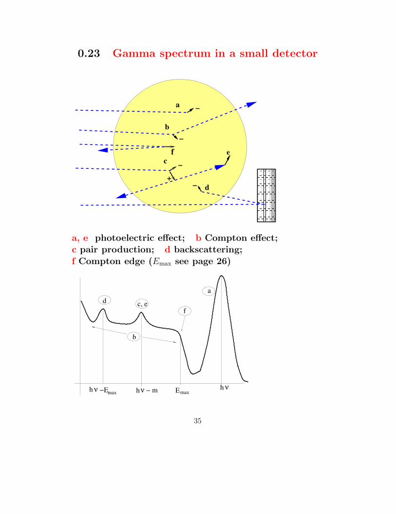
0.23 Gamma spectrum in a small detector
b
a
c
d
−
+−
−
−
ef
a, e photoelectric effect; b Compton effect;c pair production; d backscattering;
f Compton edge (Emax see page 26)
d c, e
a
f
h νhνh ν −E Emaxmax − m
b
35

Gamma spectrum in a big detector
−
+
−
−
bc
a
−
All the processes release at the end the primary γ energy
The material surrounding the detector can give:a backscattering; b 0.511 MeV annihilation γ;c X ray from photoeffect in the screen;
νh
X rayback. annih.
energyfull
peak
36
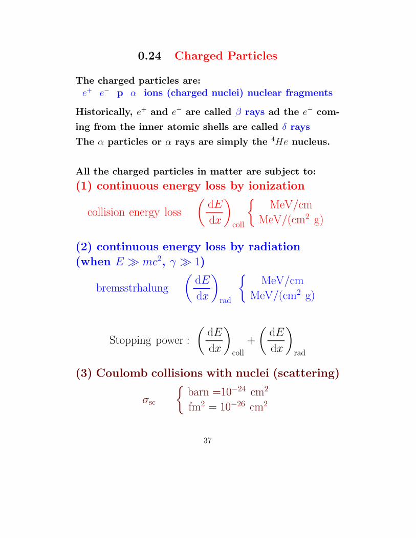
0.24 Charged Particles
The charged particles are:e+ e− p α ions (charged nuclei) nuclear fragments
Historically, e+ and e− are called β rays ad the e− com-
ing from the inner atomic shells are called δ rays
The α particles or α rays are simply the 4He nucleus.
All the charged particles in matter are subject to:
(1) continuous energy loss by ionization
collision energy loss
(
dE
dx
)
coll
MeV/cm
MeV/(cm2 g)
(2) continuous energy loss by radiation
(when E mc2, γ 1)
bremsstrhalung
(
dE
dx
)
rad
MeV/cm
MeV/(cm2 g)
Stopping power :
(
dE
dx
)
coll
+
(
dE
dx
)
rad
(3) Coulomb collisions with nuclei (scattering)
σsc
barn =10−24 cm2
fm2 = 10−26 cm2
37

0.25 Energy loss by collisions
Due to the long-range Coulomb force, the collisions withthe electrons of the absorber atoms are so numerous
that they appear as a continuous process.A collision can give the atom ionization or excitation
and these processes are used in the detectors of chargedparticles
The collision energy loss is well described by theBethe-Bloch formula:
− dE
dx=
4πe4z2NZ
mec2β2
[
1
2ln
2mec2β2γ2Tmax
I2− β2
]
= 0.3071 ρz2Z
Aβ2
[
1
2ln
2mec2β2γ2Tmax
I2− β2
] [
MeV
cm
]
z, Z are the atomic numbers of the projectile and ab-sorber atoms and
4πe4NA/(mec2) = 0.3071 MeV cm2/g (4)
me and M are the electron and projectile mass (eV)Tmax is the max energy transferred to an electron
Tmax =2mec
2β2γ2
1 + 2γme/M + (me/M)2, γ =
1√
1 − β2(5)
β = 1 − v2/c2 where v is the projectile velocityρ is the density and I is the ionization potential:
I ' 12 × Z [eV ]
All the charged particles follows this formula!
Some minor corrections at very low and very high en-ergies are necessary.
Often it is used also: dE
d(ρ x)
[
MeV cm2
g
]
38

Energy loss by collisions
The collisional energy loss has a general behaviour as
dE
dx∝ 1
v2
that is more the particle is low more the dE/ dx is high
single particle
− dE
distance of penetration
dx
parallelbeam
Bragg curve (Bragg peak)
This behaviour is more and more evident by increasing
the projectile mass and, at the same mass, for antipar-ticles (Barkas effect)
Example: 1 MeV Electron on an Al absorber
E =m
√
1 − β2= (1 + 0.511) → β =
√
1 −m2/E2 = 0.94
z = 1, Z = 13, A = 27, ρ = 2.7 g/cm3, γ = 2.93Tmax = 0.987 MeV, I = 12 × 13 = 156 eV = 156 10−6 MeV
dE
dρ x= 1.480 MeV cm2/g = 4.00 MeV/cm
(The more precise result with the density correction is 1.473 MeVcm2/g.)
39

Mixtures and compounds
dE
d(ρ x)=
∑
i
wi
[
dE
d(ρ x)
]
i
[
MeV cm2
g
]
When the total energy loss is calculated
the thickness must be expressed as the transparency.
∆E =dE
d(ρ x)ρ x
Range
R =
∫ 0
E
dx
dEdE
This integral must be done carefully or solved with asimulation
E
dxdxE dE dx E’ dE’ dx
E’
More and more thin layers are addeduntil the energy is zero.
The total path is the range
40

0.26 Radiation Energy Loss
According to Maxwell theory an accelerated (deceler-ated) charge loses energy by photon emission.
This radiation is called synchrotron radiation (from cir-cular orbits) or bremsstrahlung (motion in matter) when
a fast (γ 1) charged particle decelerates in the fieldof a nucleus partially screened by the atomic electrons.
This is as an X-ray machine works.Useful formulae for energy loss calculation (MeV/cm):
−[
dE
dx
]
rad
=0.3071E Z(Z + 1)
4 πme c2 137
ρ
A
[
4 ln2E
mec2− 4
3
]
, E < 137mec2 Z−1/3
−[
dE
dx
]
rad
=0.3071E Z(Z + 1)
4 πme c2 137
ρ
A[4 ln(183Z−1/3)] , E 137mec
2 Z−1/3
they are accurate within 10÷ 20% with the standard ta-
bles. Note the asymptotic behaviour as ' EZ2
The mean angle for photon emission is
〈θγ〉 'mec
2
E
Most of radiation lies inside a narrow cone along theincident charged particle direction. The cone is more
and more narrow with increasing the energy.
Example: electrons on Al nuclei with 1, 10, 100 MeV:
E1 = 1.511, E2 = 10.511, E3 = 100.511 MeV,Energy loss at the three energies:
dE/ d(ρx) = 0.0206, 0.335, 4.09 MeV cm2/gAccurate table values: 0.029, 0.287, 3.71 MeV cm2/g.
41

Radiation length
At high energy the bremsstrahlung follows the
rule:
−[
dE
dx
]
rad
=0.3071 Z(Z + 1)
4 πme c2 137
ρ
A[4 ln(183Z−1/3)]E ≡ 1
X0E
which implies an energy loss of the type
E = E0e−x/X0 (6)
where
X0 =4 πme c
2 137
0.3071 Z(Z + 1)A
1
4 ln(183Z−1/3)g/cm2
There is the more accurate empirical formula
of Dahl (data interpolation):
X0 =716.4 A
Z(Z + 1) ln(287/√Z)
,g
cm2
The radiation length X0 (sometimes denoted
as XR) is the mean distance over which a high
energy particle (electron) remains with a frac-
tion 1/e ' 37% of its initial energy, the remain-
der being lost by bremsstrahlung.
The radiation length is the characteristic dis-
tance for describing the electromagnetic cas-
cades.
42

0.27 Stopping Power
dE
dx=
[
dE
dx
]
coll
+
[
dE
dx
]
rad
1
10
100
Mev cm /g2
0.001 1 100.01 0.1 10 100 1000 10 4 5
Bethe Bloch
minimumionization
bremsstrahlungradiative losses
βγ
All the incident particles have a region of
minimum ionization. MIP: minimum ionizing particle:[
dE
d(ρ x)
]
MIP
' 2MeV cm2
g
for βγ ' 3.
The general rule for e+ e− collision/radiation balance:
( dE/ dx)rad
( dE/ dx)coll' EZ
1600mec2' EZ
800→ Ecrit(MeV) =
800
Z(7)
43

0.28 Positronium annihilation
e+ + e− = γ + γ
Annihilation into a single photon is possible with an
electron bound in a nucleus, but the cross section ismuch lower (< 20%). The cross section is:
σann = πe4
m2e c
4
1
γe + 1
[
γ2e + 3γe + 1
γ2e − 1
ln(γe +√
γ2e − 1) − γe + 3
√
γ2e − 1
]
where γe = E/mec2. The cross section peaks for γ = 1,
γ0 10 20 30 40 50 60 70 80
5
4
3
2
1
0
−1−2that is for positrons at rest, where the e+ e− system can
form the positronium:singlet e+ e− → 2 γ, 0.511 MeV each, lifetime 0.1 ns;triplet e+ e− → 3 γ, lifetime 100 ns;
Triplet:singlet is 3:1, but in dense media, due to thelonger lifetime, the triplet undergoes many collisions
that favour the trasition to singlet and the sudden decayinto 2 γ (2γ dominance).
44

0.29 Energy straggling (dispersion)
The stopping power in a thickness X of absorber is theMEAN VALUE of a statistical process
For the Central Limit theorem for thick absorbers (∆E/E >10%) the distribution is Gaussian.
For thin absorbers the distribution is strongly asymmet-rical with a long right tail in the lost energy (Landau
and Vavilov). The kind of the distribution is decidedby some scale parameters:
the maximum energy transfer to an electron (page 38)
Emax =2mec
2β2γ2
1 + 2γme/M + (me/M)2
the typical mean energy loss (page 38)
ξ =0.3071
2
z2Z
β2
ρ
AX MeV
the variance of the distribution
σ2E = ξ Emax
(
1 − β2
2
)
MeV2 (8)
• ξ/Emax 1: several collisions: Landau distribution
• ξ/Emax ' 1: many collisions: Vavilov distribution
• ξ/Emax 1: great number of collisions, stochasticregime, Gauss distribution
This theory assumes that ξ/I 1, that is it neglects thefluctuations in the small energy losses, and considers
only those due to δ electrons.For ξ/I < 1 there is no solution (MC simulations)
45

Landau-type curves
The Landau curve is the limit distribution of the theory
for thin absorbers: it is an universal curve both forheavy particles and electrons
The detectors give the Landau curve as a function ofthe lost energy
The left tail is ' 1.5 σThe right tail extends up to ' 9 σ and it is due to theδ electron emission.
46

Energy and range straggling
E
x
Landau
Vavilov
Gauss
Bethe−Blochcurve
single particle
− dE
distance of penetration
dx
parallelbeam
Bragg curve (Bragg peak)
47

0.30 Coulomb Multiple Scattering
x
θ
ψ
x/2
s
y
The charged particle traversing a medium experiences
the effect of the screened Coulomb field of the nuclei.Since the elastic scattering cross section behaviour '1/ sin4(θ/2), at small angles the effect is so high that itcan be treated as a continuous process givingsmall angle deflections per unit path.
The full treatment is given by the Moliere theory. An
empirical formula deduced from it gives the r.m.s. de-flection angle with an accuracy ' 10%:
θ0 =13.6 MeV
βcpz
√
x/X0 [1 + 0.038 ln(x/X0)] rad (9)
CAUTION: since this is an empirical formula with a log-
arithm, if one adds two thin media the resulting r.m.s.angle is not
√
θ201 + θ2
02. The rule is to calculate before x
and X0 (in cm2/g, as the usual weighted sum) and afterto use the formula.
48

Coulomb Multiple Scattering
x
θ
ψ
x/2
s
y
The Moliere distribution, in the small angle approxima-
tion, in the plane can be approximated with a gaussian:
1√2π θ0
exp
[
−θ2
θ20
]
dθ (10)
In space the distribution with gaussian component isgiven by the Rayleigh distribution:
1
2π θ20
exp
[
−θ2x + θ2
y
θ20
]
dθx dθx (11)
where x and y are in the plane ⊥ to the direction of
motion. In the small angle approximation:
ψ =1√3θ0 , y =
1√3x θ0 , s =
1
4√
3x θ0
49

Coulomb Multiple Scattering: electrons
Electrons and heavy particles have more or less the
same formula for the dE/ dx and the multiple scattering.However, the real behaviour, for energies around the
MeV, is completely different:
• the electron are very often relativistic and the en-ergy loss has a large bremsstrahlung component;
• the energy loss for heavy particles is mainly due to
excitation/ionization (Bethe-Bloch);
• the electrons have large multiple scattering devia-tions and their motion into a medium is “zigzagged”
(see the next photo)
50

Coulomb Multiple Scattering: electrons
51

0.31 Electromagnetic showers
52

Electromagnetic (e.m.) showers
High energy electrons radiates high energy photons andlose energy exponentially in a radiation length X0. (see
page 42)High energy photons generate high energy electrons bypair production. The mean distance is (7/9)X0.
These two combined effects are the source of the
spectacular e.m. showers.
0 1 2 3X o
+
+
+
The two important quantities are:the distance measured in radiation lengths: t = x/X0
the critical energy below which
( dE/ dx)rad < ( dE/ dx)coll (page 43)
53

Electromagnetic showers
The structure of an e.m. shower triggered by
a particle (electron or photon) with energy E0
is:
• number of particles after t radiation lengths
N(t) ' 2t
• distance with shower energy Et:
t(Et) = ln(E0/Et)/ ln 2
• distance with the maximum number of par-
ticles. This roughly is the shower depth,
because after this point the shower abruptly
stops.
tmax =lnE0/Ec
ln 2We see that the shower depth increases
logarithmically with the primary energy.
• the mean number of particles (e+, e−, γ)
is Nmax = E0/Ec and is proportional to the
primary energy.
e.m. showers occur in “normal life” by cosmic
rays and artificially in the particle accelera-
tors.
54

A 1 Gev γ shower
< −1m −− >
γ rays, charged particles14 Copper slabs 1 cm thick, X0 = 1.43 cm,
Ec = 27 MeV, tmax = 5, xmax = 7.45 cm, ' 8 slabs
55

A 1 Gev γ shower
2 m × 2 m calorimeterγ rays, charged particles
56

0.32 Cherenkov radiation
A particle with constant velocity does not radiate. How-ever, the electrons of the medium feel a variable e.m.
field, they accelerate/decelerate and emit a small amountof radiation. This effect is a negligible contribution to
the particle energy loss.However, when the particle velocity exceeds the light
velocity in a medium of refractive index n
v >c
n, → β >
1
nthe coherent wavefront of the Cherenkov light can bedetected (think to a fast ship in water...)
θ
c/n
v
wave front
v<c/n v>c/n
cos θc =c
n v=
1
n β
The number of γ per unit path length and per energyinterval is
d2N
dE dx=αz2
csin2 θc ' 370 z2 sin2 θc eV−1 cm−1
57

0.33 Nuclear Interactions
Differently from the e.m. interactions,the nuclear interactions due to the shortrange strong force give rise to discreteprocesses.
The e.m. interactions are forward peaked.Away from the forward direction, themain effects are due to the strong (nu-clear) interaction.
Remember the connection between eventrate and the cross section (page 18):
# collisions
s= σISXN = σISX
ρNA
A(12)
Cross sections are related to nuclearradius. In a blob of constant densityone has (4/3)πr3 ∝ A, therefore;
r = r0A1/3 where r0 ' 1.25 10−13 cm
58

Nuclear Interactions
The general behaviour of the cross section is
σt = σel + σabs
From Quantum Mechanics, the scattering cross
section at low energy is 4 times the geometri-
cal cross section:
σel = 4 π r2 = 4 π r20 A
2/3
The capture cross section at low energy hasthe 1/v behaviour
σabs =Γ
(E −E0)2 + Γ2/4→ c√
E
1/vresonance
σ
E
typical neutron cross section
σt = 4 π r2 +c√E
59

0.34 Interaction matter-radiation: summary
Resonant capture
Coulomb multiple scattering
Energy straggling
Photoelectric effect
Compton effect
e+e− pair production
e+ e−
proton
gamma
neutron proton
, heavy
heavy particles Elastic scattering
1/v capture
charged particles
(ionization)dE/dx
e+ e− annihilationdE/dx (bremsstrahlung)
Magnetic deflection
Cherenkov (relativistic v>v )c
nuclear
e.m.
60
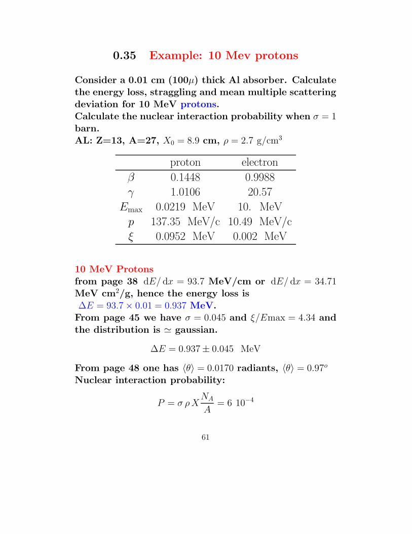
0.35 Example: 10 Mev protons
Consider a 0.01 cm (100µ) thick Al absorber. Calculatethe energy loss, straggling and mean multiple scattering
deviation for 10 MeV protons.Calculate the nuclear interaction probability when σ = 1
barn.AL: Z=13, A=27, X0 = 8.9 cm, ρ = 2.7 g/cm3
proton electron
β 0.1448 0.9988
γ 1.0106 20.57
Emax 0.0219 MeV 10. MeV
p 137.35 MeV/c 10.49 MeV/c
ξ 0.0952 MeV 0.002 MeV
10 MeV Protons
from page 38 dE/ dx = 93.7 MeV/cm or dE/ dx = 34.71MeV cm2/g, hence the energy loss is
∆E = 93.7 × 0.01 = 0.937 MeV.From page 45 we have σ = 0.045 and ξ/Emax = 4.34 and
the distribution is ' gaussian.
∆E = 0.937± 0.045 MeV
From page 48 one has 〈θ〉 = 0.0170 radiants, 〈θ〉 = 0.97o
Nuclear interaction probability:
P = σ ρXNA
A= 6 10−4
61

0.36 Example: 10 MeV electrons
Consider a 0.01 cm (100µ) thick Al absorber. Calculatethe energy loss, straggling and mean multiple scattering
deviation for 10 MeV electrons.AL: Z=13, A=27, X0 = 8.9 cm, ρ = 2.7 g/cm3
proton electron
β 0.1448 0.9988
γ 1.0106 20.57
Emax 0.0219 MeV 10. MeV
p 137.35 MeV/c 10.49 MeV/c
ξ 0.0952 MeV 0.002 MeV
10 MeV Electronsfrom page 38 dE/ dx = 4.78 MeV/cm or dE/ dx = 1.77
MeV cm2/g, hence the collision energy loss is∆E = 4.78 × 0.01 = 0.0478 MeV.From page 41 dE/ dx = 0.640 MeV/cm by bremsstrahlung
and ∆E = 0.640× 0.01 = 0.0064 MeV.Total energy loss ∆E = 0.0478 + 0.0064 = 0.0542 MeV.
From page 45 we have σ = 0.10 and ξ/Emax 1 so thatthe distribution is Landau-type (note the large fluctua-
tions):
∆E = 0.054± 0.100 MeV
From page 48 one has 〈θ〉 = 0.0322 radiants, 〈θ〉 = 1.85o
62

0.37 The Monte Carlo method
• It originates at Los Alamos by anidea of J. von Neumann and S.Ulam,to treat scattering and absorption ofneutron in fissile materials.
• from the 50-ies there is a big diffu-sion of the method, thanks to com-puters
• presently it is one of the more im-portant methods of nclear physics
• the method is based on two funda-mental ideas: the cumulative vari-able theorem, and the Central Limittheorem. Based on this, only anuniform random number generatoris necessary
ξ ∼ U(0, 1)
63

0.38 The sampling technique
Theorem 1:
If a ≤ X ≤ b, e X ∼ U(a, b)
Px1 ≤ X ≤ x2 =1
b− a
∫ x2
x1
dx =x2 − x1
b− a. (1)
If (1) is valid, then X ∼ U(a, b)
Theorem 2:
If X has a continuous density p(x) the cumu-
lative random variable
C(X) =
∫ X
−∞p(x) dx
is uniform in [0, 1], that is C ∼ U(0, 1).
Example: simulate a nuclear event when
σsc = 2 barn and σabs = 3 barn.
If RANDOM < 0.4 there is scattering, otherwise
absorption occurs.
scattering absroption
0 0.4 1
Figure 1: Simulation of thr scattering-absorption mechanism with the routinerndm.
64
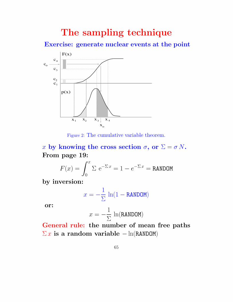
The sampling techniqueExercise: generate nuclear events at the point
x
c
xxx
c
3
c4
p(x)
F(x)
ox
o
2
1
c
4321
c
Figure 2: The cumulative variable theorem.
x by knowing the cross section σ, or Σ = σ N .
From page 19:
F (x) =
∫ x
0
Σ e−Σ x = 1 − e−Σ x = RANDOM
by inversion:
x = − 1
Σln(1 − RANDOM)
or:
x = − 1
Σln(RANDOM)
General rule: the number of mean free paths
Σ x is a random variable − ln(RANDOM)
65

0.39 Rejection method
xi = a + ξ1(b− a)
yi = ξ2h
with 0 ≤ ξ1, ξ2 ≤ 1.
Accept xi if yi < p(xi)
h
a b
p(x)
X
p(x )
x i
i
Figure 3: The rejection technique.
66

0.40 Sampling examples
Uniform sampling into a circle:
p(ϕ) dϕ =ρR2 dϕ/2
ρπR2=
dϕ
2π.
For q(r) we have
q(r) dr =ρ2πr dr
ρπR2=
2r
R2dr .
The correspondnig cumulatives are:
ξ1 = P (ϕ) =
∫ ϕ
0
p(ϕ) dϕ =ϕ
2π,
ξ2 = Q(r) =
∫ r
0
q(r) dr =r2
R2.
ϕ = 2πξ1r = R
√ξ2 .
67

Sampling examplesIsotropy
x = R senϑ cosϕ
y = R senϑ senϕ
z = R cosϑ .
dΩ = senϑ dϑ dϕ .
If ntot is the number of points:
ntot4π
=dn
dΩ, isotropy
We have:
p(Ω) dΩ =dn
ntot=
dΩ
4π=
senϑ dϑ dϕ
4π
p(ϕ) dϕ =1
4πdϕ
∫ π
0
senϑ dϑ =1
2πdϕ ,
q(ϑ) dϑ =1
4πsen ϑ dϑ
∫ 2π
0
dϕ =sen ϑ
2dϑ .
The corresponding cumulatives are:
ξ1 = P (ϕ) =ϕ
2π,
ξ2 = Q(ϑ) =1 − cosϑ
2
ϕ = 2πξ1ϑ = acos(1 − 2ξ2) .
68
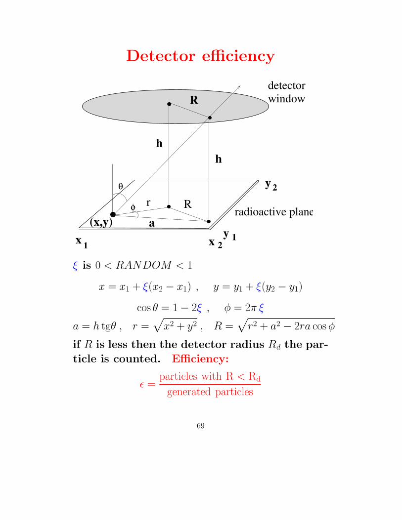
Detector efficiency
θ
φ Rr
R
hh
y
y
xx 1 21
2
a(x,y)radioactive plane
detectorwindow
ξ is 0 < RANDOM < 1
x = x1 + ξ(x2 − x1) , y = y1 + ξ(y2 − y1)
cos θ = 1 − 2ξ , φ = 2π ξ
a = h tgθ , r =√
x2 + y2 , R =√
r2 + a2 − 2ra cosφ
if R is less then the detector radius Rd the par-
ticle is counted. Efficiency:
ε =particles with R < Rd
generated particles
69

References
• G.F. Knoll
Radiation Detection and Measurement, John
Wiley, 1989
• R. Fernow,
Introduction to experimental particle physics,
Cambridge University Press, 1990
• E. Segre
Nuclei e Particelle, Zanichelli, 1896
• http://hyperphysics.phy-astr.gsu.edu/hbase/hframe.html
70


