SLAC-PUB-5381 November 1990 T

ALCHEMY IN 1 + 1 DIMENSION: FROM BOSONS TO FERMIONS

H. GALI~* t

Stanford Linear Accelerator Center

Stanford University, Stanford, California 94309

ABSTRACT

Canonical massless fermion field is constructed from canonical boson field in

1 + 1 dimensional space. Single-fermion states are expressed in terms of eigenstates

of boson operators.

Submitted to American Journal of Physics

* Work supported by the Department of Energy, contract DE-AC03-76SF00515. t e-mail address: galic@slacvm.bitnet

1. INTRODUCTION

Matter is made of fermions and bosons. Spin and statistics is what makes a

difference between the two. Fermions are characterized by half-integer values of

spin, and by the Pauli exclusion principle. They are described by sets of quantum

operators with simple anti-commuting rules. Bosons, on the other hand, have in-

teger values of spin, a state can contain an arbitrary number of bosons with the

same. quantum numbers, and commutators rather than anticommutators charac-

terize the corresponding operators. It is well known from the statistical, nuclear,

and particle physics that an even number of fermions can form a boson. For exam-

ple, quark-antiquark pairs (Le., pairs of fermions), are believed to compose mesons

(which are bosons). This is really not a surprise: if some binding force keeps an

even number of objects with a half-integer spin together, it must be possible to

combine them into an object with an integer spin. Along these lines one might even

tend to believe that fermions are perhaps more fundamental objects than bosons,

and consider the latter merely as composed states.

However, such a view neglects among other things the fact that the oppo-

site direction is also possible: fermions may be made out of suitably arranged

bosons, at least in a lower dimensional space! The present article deals just with

such a surprising relationship between fermions and bosons in the one-dimensional

space. During the past thirty years this subject was thoroughly studied by many

distinguished physicists, and with a good reason. The transformation of bosons

to fermions and vice versa (or the “bosonization” of fermions, as it is sometimes

called) might prove to be a very useful tool in getting a valuable insight into the

long-standing problem of confinement in the quantum chromodynamics. The con-

cept was also used to solve complicated, interacting models in 1 + 1 dimension,

by replacing them with simpler and/or non-interacting theories. Furthermore, the

mere notion that fermions and bosons are deeply inter-related, has a beauty on its

own. Yet, students are most often exposed to the subject only in highly specialized

graduate courses. E.g., the popular introductory-level textbooks on quantum field

2

theory very rarely mention the bosonization. Similarly, in the last decade there

was not even a single article on the topic in this Journal.

This paper is meant to be an elementary introduction to the fermion-boson

duality. It considers the simplest possible situation: the world is reduced to one-

dimensional segment of a finite length, and we study the possibility of forming

free fermions in the segment, by using only the free, massless bosons. Truly, in

one-space, one-time dimension (1 + 1) th e angular momentum is not defined, and

we-do not have to worry about the spin, but fermions and bosons are still distin-

guishable by their statistics. Our task is therefore to find the transformation from

a set of commuting operators characterizing bosons, into another set of anticom-

muting operators corresponding to fermions. But why would anyone want to know

anything about such a simplified world in which some non-interacting particles are

kept in a segment ? First, the finite length of the interval is really not a serious

restriction. This length is an infra-red cutoff which can be set to infinity at the

end of the analysis. Furthermore, the free and massless theory in 1 + 1 dimension

is simple enough to be easily absorbed by beginners and non-experts, and yet it

contains almost all important elements needed in a more advanced study of mas-

sive and interacting systems. Once the interactions are introduced, the whole new

world opens, and not only of the pure academic interest. For example, a better

understanding of interacting one-dimensional systems might prove crucial for the

development of synthetic metals, new types of transistors, or light-weight, recharge-

able, high-energy-density batteries. More on these possibilities in the concluding

section.

This article is primarily aimed at the first and second year students of graduate

schools, but an undergraduate with some knowledge of relativistic quantum me-

chanics, and inclined to quantum field theory or condensed matter physics, could

also benefit from it. Those readers not interested in the relativistic quantum fields,

can neglect all the dynamics and consider this paper an exercise in transforming

commuting into anticommuting variables within the framework of ordinary quan-

tum mechanics. We begin by finding a general solution @(t, Z) of the Klein-Gordon

3

equation dJ‘“d,@ = 0 in a segment of a finite length L. The field @ is described in

terms of various time-independent operators, and the operators satisfy simple com-

mutation rules (Section 2). The time evolution of “physical” states is determined

by hamiltonian and the momentum operator, which are constructed in Section 3.

The one-dimensional Dirac equation iypa,!P = 0 , and general properties of a

fermion field operator Q(t,x) in a segment of length L, are studied in Section 4.

Section 5 is the heart of this article: we use boson operators to construct the

fer-mien field, and show that field operators in the resulting set satisfy the correct

anticommutation rules. We then express fermionic annihilation and creation op-

erators in terms of the bosonic counterparts, and discuss single particle states for

fermions (Section 6). Delta functions relevant to finite intervals are described in

Appendix A, and a brief review of the Klein’s factor can be found in Appendix B.

In preparing this paper I benefited most from the two articles by Wolf and

Zittartzt’] in which one can also find a good list of references to the earlier works

as well as the discussion on the relevance of the subject for the solid state and sta-

tistical physics. The articles by Boyanovsky:’ Kogut and Susskindy’ and Klaibery]

were also very useful in my study. For the lattice version of the problem see e.g.,

the article by Shultz, Mattis and Lieb15]. I truly enjoyed following this miraculous

transformation of bosons to fermions, and hope that the readers will also find it

exciting.

2. KLEIN-GORDON EQUATION

To begin, we consider the equation

(&g)rn(r_.)=O (1)

in the segment x E [-L/2,+L/2] , f or a real function @(t,x). The form of the

equation (1) allows us to introduce the “charge density” p(t, x) = fD’(t,x)/J”,

and the “current” J(t, x) = -$(t,x)/fi , where “prime” and “dot” denote

4

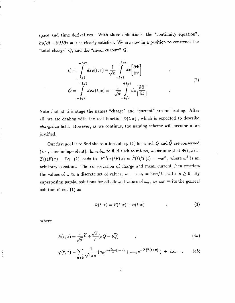
space and time derivatives. With these definitions, the “continuity equation”,

+/at + &J/ax = 0 is clearly satisfied. We are now in a position to construct the

“total charge” Q, and the “mean current” 0,

+Ll2 +J5/2

&= J dxp(t, x) = L fi J [I dx g

da: -L/2 -L/2

dxJ(t,x) = - L 1/;; J II d!!!! x at -L/2 -L/2

(2)

Note that at this stage the names “charge” and “current” are misleading. After

all, we are dealing with the real function @(t, x) , which is expected to describe

chargeless field. However, as we continue, the naming scheme will become more

justified.

Our first goal is to find the solutions of eq. (1) for which Q and Q are conserved

(i.e., time independent). In order to find such solutions, we assume that @(t,x) =

T(t)F(x) . Eq. (1) leads to F”(x)/F(x) = f’(t)/T(t) = -w2 , where w2 is an

arbitrary constant. The conservation of charge and mean current then restricts

the values of w to a discrete set of values, w + wn = 2m/L , with n 2 0 . By

superposing partial solutions for all allowed values of wn, we can write the general

solution of eq. (1) as

w, 4 = w, 4 + cp(t, 4

where

R(t,x) =&F +$(x& - tij) 7

(3)

(44

cp(t, X) = C 1 (anemi%?CtB2) + a-ne-iF(t+zJ ) + C.C, . n>O G

w

5

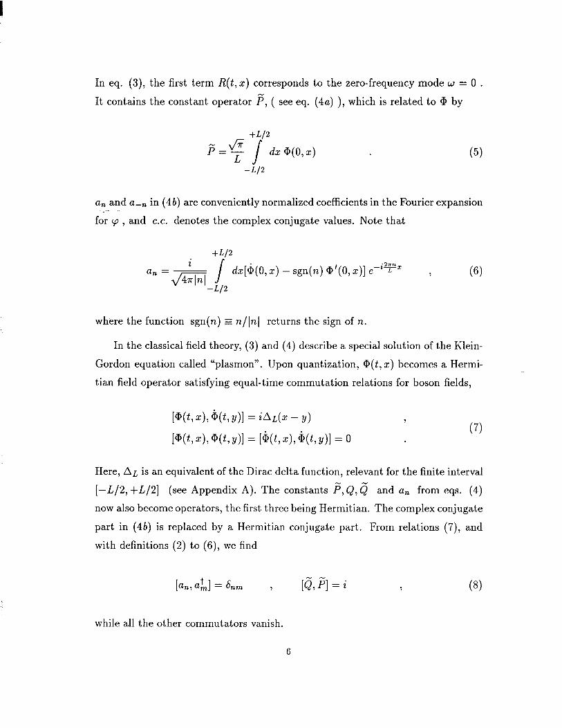
In eq. (3), the first term R(t, x) corresponds to the zero-frequency mode w = 0 .

It contains the constant operator P, ( see eq. (4~) ), which is related to @ by

+L/2 6 p”CT

J dx @(O, x)

-L/2

(5)

a, and a-, in (4b) are conveniently normalized coefficients in the Fourier expansion

for ‘p , and C.C. denotes the complex conjugate values. Note that

dx[b(O, x) - sgn(n) @‘(O, x)] e-‘FZ , (6)

where the function sgn(n) E n/In] returns the sign of n.

In the classical field theory, (3) and (4) describe a special solution of the Klein-

Gordon equation called “plasmon”. Upon quantization, Q(t, x) becomes a Hermi-

tian field operator satisfying equal-time commutation relations for boson fields,

[%x),&y)] = ~AL(x - y) ,

P(t, IL'>, w, Y)] = [W, x), qt, Y)] = 0 (7)

-

Here, AL is an equivalent of the Dirac delta function, relevant for the finite interval

w/2, +Wl ( see Appendix A). The constants F,Q, Q and a, from eqs. (4)

now also become operators, the first three being Hermitian. The complex conjugate

part in (4b) is replaced by a Hermitian conjugate part. From relations (7), and

with definitions (2) to (6), we find

ian7 uk] = &cm 7 [ij,P]=i (8)

while all the other commutators vanish.

6

As we might have expected, the boson field is described by an infinite set of

harmonic oscillators with frequencies wn = 2r[nj/L, and characterized by annihi-

lation and creation operators a, (a;), acting in the Hilbert space S, . In addition to

these local degrees of freedom, there are other, global operators in the expansion of

the field. These are Q with its conjugate pair F, and the operator Q. We usually

neglect those operators when the value of x is unrestricted, but in the final interval

they do play a central role. Since the global operators Q and Q commute mutually

as-well as with all an(ak) operators, they generate two new Hilbert spaces, SQ

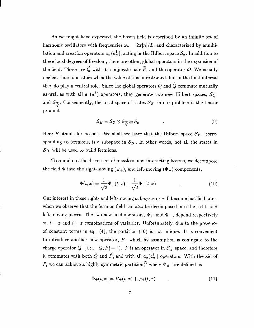
and Sa . Consequently, the total space of states SB in our problem is the tensor

product

Here B stands for bosons. We shall see later that the Hilbert space SF , corre-

sponding to fermions, is a subspace in Sg . In other words, not all the states in

SB will be used to build fermions.

To round out the discussion of massless, non-interacting bosons, we decompose

the field @ into the right-moving (@+), and left-moving (@-) components,

qt, x) = +D+(t, x) + $L(t, z) . (10)

Our interest in these right- and left-moving sub-systems will become justified later,

when we observe that the fermion field can also be decomposed into the right- and

left-moving pieces. The two new field operators, @+ and a,_ , depend respectively

on t - x and t + x combinations of variables. Unfortunately, due to the presence

of constant terms in eq. (4), the partition (10) is not unique. It is convenient

to introduce another new operator, P , which by assumption is conjugate to the

charge operator Q (Le., [Q, P] = i). P is an operator in SQ space, and therefore

it commutes with both Q and P, and with all a,(& ) operators. With the aid of

P, we can achieve a highly symmetric partition:] where @& are defined as

7

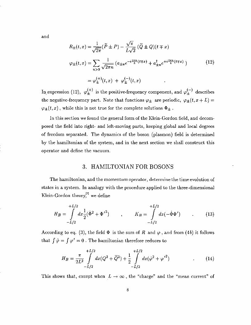
and

p*(t, X) = C L (afnemiYCtTz) + u~ne+i~(Q-~) )

n>O G (12)

= &‘(t,x) + &‘(t,x) In_ expression (12)) (p!+’ C-1 is the positive-frequency component, and ‘p* describes

the negative-frequency part. Note that functions cp* are periodic, cp*(t, x + L) =

cp*(t, x) , while this is not true for the complete solutions Qi* .

In this section we found the general form of the Klein-Gordon field, and decom-

posed the field into right- and left-moving parts, keeping global and local degrees

of freedom separated. The dynamics of the boson (plasmon) field is determined

by the hamiltonian of the system, and in the next section we shall construct this

operator and define the vacuum.

3. HAMILTONIAN FOR BOSONS

The hamiltonian, and the momentum operator, determine the time evolution of

states in a system. In analogy with the procedure applied to the three-dimensional

Klein-Gordon theory:” we define

i-L/2

HB = J

dx;(i2 + (a’2)

-L/2

,

+L/2

IcB = J

dx(-it@‘) .

-L/2

(13)

According to eq. (3), the field Q, is the sum of R and ‘p , and from (4 b) it follows

that J(j=Jcp’=O.Th e h amiltonian therefore reduces to

+-L/2 +L/2

HB= & J dx(Q2 + G”) + f .I dx((p2 + (P’~) -i/2 -i/2

This shows that, except when L -+ 00 , the “charge” and the “mean current” of

8

a state also contribute to the total energy. Since the second integral in eq. (14)

represents the standard harmonic contribution, we can immediately write

HB=&(Q2+~2)+~wn(a!a,+~) . n#O

(15)

In eq. (15), wn = 2rlnl/L is the frequency (and, at the same time the energy) of

the massless harmonic excitations. The expression still contains an infinite energy

of the vacuum, a C wn, which should be subtracted. As a convenient shorthand for

this subtraction we introduce the normal ordering with respect to the SB vacuum

state. For an operator X , let iXi denotes

:x:=x-(01X10) , (16)

where I 0 ) is the state with zero charge and mean current, Q I 0 ) = Q I 0 ) = 0 ,

and no oscillators, a, I 0 ) = 0 . Using this definition, we may now express the

normalized hamiltonian for bosons as

+L,2

HB = i J

dxi(&2+@12) i = &(Q2+Q2)+Cwnaian .

-L/2 n#O (17)

In the tensor product notation we can describe the vacuum state as

(18)

Here, IO), d enotes an eigenstate of Q with the eigenvalue zero, Q IO), = 0 .

Similarly, Q IO) - = 0, and an IO), = 0 Q f or all allowed values of n. By construction,

I 0 ) is the state with the lowest energy, HB I 0 ) = 0.

We can excite the vacuum IO), in S, , by applying the creation operators in

the standard way. E.g., for an arbitrary integer value of n, we can form single

particle states of the frequency wn , by constructing the vectors a! IO), G la,), or

9

at, IO), E (a-,), . Th e si ua ion is slightly different in SQ and Sa subspaces. ‘t t’

While in S, the frequencies of oscillators are quantized, here we find no restrictions

to the values of Q and Q. Consequently, both may assume arbitrary real eigenvalues

from --oo to +oo . In order to create various non-zero eigenstates of Q and Q , it

is convenient to use the conjugate operators P and P . E.g., consider the state

b)Q = exP(-iqP) lo), - It is easy to see that Q lq)Q = q 1q)Q , and thus, 1q)Q is

indeed an eigenstate of Q with the eigenvalue q . The proof is left as an exercise

for. the reader. In a similar way, starting with IO),- , and by making use of

conjugate operator P , we construct all the eigenvectors of Q .

In analogy with the procedure applied to hamiltonian, we also subtract

momentum of the vacuum from the momentum operator in (13), and write

+-L/2

the

the

I-B = : J d5(-&v) i = ; Qa + c k&n, (19) -L/2 n#O

where k, = 2mx/L is the momentum corresponding to the excitation ai IO), . The

second term in (19) is the standard harmonic contribution. From the first term we

find again that for any finite length L, the charge and current modify values of the

operator.

-

In this section we defined the vacuum I 0 ) as a tensor product of states with

zero charge, zero mean current, and with no harmonic excitations. Having con-

structed the vacuum, we renormalized the hamiltonian and momentum operator by

subtracting corresponding vacuum expectation values. Next, we turn our attention

to fermions.

10

4. HOW SHOULD FERMIONS LOOK?

In 1 + 1 dimension, the Dirac equation for massless fermions is

+i od a

dt + rljjp(t, 2) = 0 3

where in the “chiral” representation,

For the components Q& , we find that

d d (at f gw’“) = 0

(20)

(22) Consequently, it becomes clear that 9+ is a function of t - 17: combination, and

describes a propagation in the positive (right) d irection along the x axis, while the

Q- is a function of t + x , thus corresponding to propagation in the negative (left)

direction.

We are interested in a particular set of solutions of eq. (22), which satisfy

anti-periodic boundary conditions, XP*($, t) = -Q&(-t, t) . Namely, it turns out

that for such anti-periodic solutions we can most easily accomplish the intended

transformation of bosons into fermions. Given the boundary conditions, we can

write the general solutions of eq. (22) as

9*(t, x) =& E(O*), eWn+9(-) , -CO

(23)

where (0-t )n and (D- )n are appropriately normalized constants defined by

+L/2

(&)n = & / d17 e-i%n+f)q ~~(0, ‘I) -L/2

. (24)

We can now quantize the theory. The main difference from the procedure in the

Klein-Gordon theory is our use here of anticommutators instead of commutators.

11

We require that

{Qlr(C x:), w+(t, Y)) = &T1 ;IL(X, Y) , (r,d = *) (25)

with all the other anticommutators vanishing. In (25), AL is an antisymmetric

delta function which is described more thoroughly in the Appendix A. The differ-

ence between AL and AL lies in the fact that AL(X) + 00 when x + fL ,

while in the same limit AL(X) + --oo . In the limit L --t cc, both AL and AL

are replaced by the ordinary Dirac delta function 6(x) . We point out that the

antisymmetric fields 9* require an antisymmetric delta function in (25).

Upon quantization, the constants (24) t urn into operators whose algebra is

assigned by the anticommutators (25). It is convenient to replace operators in (24)

by a set of new operators

4-L/2

bn>o = (O+)n = -L a J

dxe-“%n+i)” Q+(o, x)

-L/2

i-L/2

b n<O = (II-)n = & J dxe-“~(“+f)” Q-(0, X)

-L/2

-kL/2

dn>o = (o+)i-,wl = L a J

dxe-“%++)” I$ (0, x)

-L/2

-l-L/Z

d n<O = (D-)tnT1 =A / dxe-“?‘(“++ !$(O,x)

-L/2

.

The new operators have simple anticommutators,

{bn, bi} = {dn, dk} = ham 7

(26)

(27)

as we verify by direct calculation. All the other anticommutators of operators

in (26) vanish. We recognize the operators (26) as the annihilation operators

12

for fermions. Likewise, the hermitian conjugates of (26) are fermionic creation

operators. From (23) we obtain

Q+(t, x) = s& g (bne-“i”b+t)@-“) + df,e’y(n++)(-) ) , n-0

(28)

q-(t, 2) = .& z (b-ne-"i"(n-b)(t+z) + dinei?(n-+)(t+") ) .

n-l

Consequently, for non-negative values of n, b, and b! are annihilation and creation

operators for the right-moving massless fermions with energy cn = 27r(n + $)/L .

Similarly, d, and di correspond to the right-moving massless antifermions. For

n < 0, the corresponding operators describe left-moving fermions and left-moving

antifermions. We are now in the position to define the fermion vacuum, 140) . This

is the state for which bn 140) = 0 and d, I&) = 0 , for all values of n .

We can also introduce the hamiltonian and the momentum operator for the

system of massless Dirac particles. They are readily constructed in parallel with

the three-dimensional theoryL7’,

+L/2

HF =: J

dx[iQ+(t, x)i!(t, x)]:

-L/2

+L/2

IcF =: J dx[-iQ+(t, x)Q’(t, xc>]:

-L/2

.

(29)

Columns in (29) d enote the normal ordering with respect to the fermion vacuum

160) . With the aid of (28), HF and KF may be rewritten as

HF =? E In+:/ :[bibn-dndL]:= E cn(bftbn+dkdn) , n=-co n=-co

~~F=~ E (n+i) :[bLbn-dndL]:= E &(bLb,+dkd,) ,

(30)

n=--00 12=-m

where & = $F(n + i) is the momentum of the n-th excitation, and cn = lenI its

13

energy.

The charge and axial charge of the fermions can also be defined in the standard

way: q = : J dxQ+Q : , and 4 = : J dxQty”y19 : . It turns out that the

newly-defined operators satisfy

Therefore, !P+ operator decreases the charge and the axial charge by one unit.

Similarly, q- operator changes the charge for -1 unit, and axial charge for +l

unit.

In this section we analyzed general form of the solutions of Dirac equation for

massless particles. We expressed the fields and the dynamic observables in terms of

creation and annihilation operators. In the next section we demonstrate that there

are many similarities between the components q*(t,x) and the combinations of

plasmon fields, exp[fifi@*((t, x) ] .

5. FROM BOSONS TO FERMIONS

In Section 2, we constructed operators Q and Q from the current-like structure

Pa. We called them “charge” and “mean current”, although the field @ was real,

and - consequently - the plasmons were chargeless. In this section we show that

these global degrees of freedom in the expansion of the plasmon field really become

the charge and mean current (or “axial charge”) of the newly created fermions.

Anticipating the result, and knowing that the charge and the mean current can

assume only some discrete values, we restrict our analysis to a subspace of the total

Hilbert space SB .

The subspace, which we name SF (F for fermions), consists of those states

- from SB for which both Q and Q have integer eigenvalues, and Q - Q is an even

number. This condition may be rewritten as Q - Q + 2n , Q + Q + 2m ,

14

where n and m are arbitrary integers. This simply says that if fermion states are

to have integer charges, then the resulting currents may differ from the charges

only by an even number of units. We immediately observe that the vector ] 0 ) ,

which describes the plasmon vacuum, is one of the vectors in the subspace SF .

Having defined the new Hilbert subspace SF c SB , we made the first step

in the construction of fermion fields from the boson counterparts. Next, we recall

two useful operator relations:’

B Ae =e B (A+bWl) (324

eAeB = eBeA elA,Bl = ,A+B ei[A,B] > (3W which are valid if the commutator [A, B] is a number, and not another operator.

With the aid of (32), ‘t 1 is straightforward to prove that

and

(33)

(35) The new combinations, exp[fi&&*], transform eigenstates of Q to eigenstates

of Q - 1 (relation (33) ), change th e values of the mean current by - 1 (+l) unit

(relation (34) ), and satisfy the Dirac equation (35). Although these are exactly

the properties we expect of the components XP* of fermion fields (compare to eqs.

(31) and (20) ), the operators exp[fi&@*] are not yet the right combinations.

Namely, they turn out to be incorrectly normalized. Instead, we introduce the

operators

(36)

Here, T denotes + or - signs, and vT C-1 ( p$+’ ) are negative- (or positive-)

15

frequency components of the operators qk((t, x) ( see eq. (12) and below ). The

operators (36) d’ff 1 er only slightly from those used in expressions (33) to (35): the

normalization constant l/a is added, and the exponent i&r( R, +cp$-)+cp$+)) is

factorized into three separate exponents. We observe that in the new arrangement

(36) all creation operators at( are to the left of annihilation operators a, . As

a convenient shorthand for such an ordering , we may introduce the Na symbol,

and write xr(t, x) = Nh ( eir 6% )/a . The changes introduced in (36), as

we-shall see, improve the normalization without affecting the Dirac equation and

the commutators with Q and Q in (33) and (34). Consequently, operators (36)

become prime candidates for the description of fermions. It only remains to check

the equal-time anticommutators of the operators x+ and x- .

To do that, we first consider the product x7(t) 5)X!@, y) . With the aid of (32b),

we write

t ’

(37) In an analogous way we rewrite the product xi(t, y)xT(t, x) as

XtxT = $~(TR~-s&) ,i&%(Tp~-‘-~+9$-‘) ei&(Tp$,+)-sW$+)) x 5 L

(38) e--7s~[Rr,Rs] e2TS4~~+),9$-)]

7

By (8), the commutators in eqs. (37) and (38) are

16

[RT@, x), &@, y) ] = &TS ’ ;cx - Y> ,

[ p i+)(t, 2) , cp!-)(t, 7J) ] = -&cTTs C b eiTT(‘-y)

n>O

,

[ +9$+)(l, y), cp!-)(t, X)] = &b,, C A. emi %FT(‘-Y) n>O

n

(39)

and they all have zero value when the signs of r and s are not equal. Consequently,

for r # s , expressions (37) and (38) coincide, and we find the troublesome result

that a commutator instead of an unticommututor vanishes,

[XT@, x), &, y)] = 0 (for r # s) .

The situation looks less unpleasant for r = s , because we shall be able to combine

(37) and (38) ’ t m o an anticommutator (see below). However, the right hand side in

the resulting expression gets much more complicated than we m ight have expected.

Indeed, with the aid of (A.8), and by using (37) to (39), we can write for r = s,

{xTkx:>, ?&, Y>> = ei& T[&(Q)-K-(CY)I nl, e"6 T[k'r(+)-Q'r(t,Y)l zL(x _ y) .

>

(41)

The alarm caused by this expression is lessened when we observe that the term

n/,(. . .) in fact reduces to one, due to the presence of EL(x- y) function. W e verify

this in a direct calculation, by noticing that within the range of interest LL(X - y)

contains 6(x-y-L),S(x-y) and 6(x-y+L) t erms (see Appendix A). On the other

hand, the functions cpT(t, Z) are periodic, and particularly, (Pr(t) X&L)-pT(t, x) = 0.

Therefore, indeed n/a(. . .) + 1 . There is another exponential factor on the

right hand side of (41) h h w ic we would like to see eliminated. Now it becomes

crucial that the analysis is carried out in the SF subspace. Namely, by (la),

ifi r [RT(t, x) - R,(t, x f L) ] = F ia(Q + T Q) . But, since Q + Q and Q - Q

17

combinations have even eigenvalues in the subspace, the remaining factor in (41)

also takes the value of one. The anticommutator (41) is now simply

{x7, xf } = ( 6(x - y) - eir(6+TQ)b(x - y - L) - e-iX(Q+TQ)6(x - y + L) + . . .)

- LL(z - Y) (42)

Therefore, for r = s, in contrast with the r # s case (eq. (40) ), the anticommutator

of--XT- and xl operators looks fine, and we can claim at least a partial success.

We turn next to the product x7(t) x)xs(t, y) . Th ere is a complete parallel here

with the previous discussion, and we readily find that for r # s ,

kT(t~ xc>, X&T Y)] = 0 , (43)

and for r = s ,

{XT(~,X),XT(~,Y)) = 0 . (44)

Again, a commutator instead of an anticommutator appears for T # s , while for

T = s , the expression has the form corresponding exactly to the Fermi statistics.

Our attempt to determine the equal-time anticommutators of xT operators

apparently met some serious difficulties. In expressions (40) and (43), a wrong

sign appeared between combinations of operators. However, the solution of this

particular problem turns out to be very simple. To accomplish the sign change

in (40) and (43), and at the same time preserve the relations (42) and (44)) we

only have to multiply xT by a suitably chosen “Klein’s factor”. The procedure is

thoroughly explained in the Appendix B. According to the prescription, we change

XT@, Xc> + exp[irQ(l+4/2] XT(~, X) = QT(t, Xc>, and finally obtain a set of fields

obeying the correct anticommutation rules for all values of T and s ,

@jT(h xc>, Q:(t, Y)} = STS&(x - Y> 7 (45)

iqT(h x>, ‘&Y>> = o

The newly created operators !P*(t, x) therefore have all the properties required of

18

the fermion fields. They satisfy the Dirac equation for components, change charge

and current for one unit, and yet, are entirely expressed in terms of boson operators.

The “miraculous” transformation of bosons into fermions is thus achieved: fermions

become a kind of collective excitation modes of bosons.

In concluding this discussion of the transformation, we present the expression

for the Fermi field with the main parts factorized in two different ways. The

transition from one form to the other is readily achieved with the aid of (32).

eirQ ,i(P+F) e-i5(Q+e-l)(t-z) ,+i&Gp$-’ ,+i&Gpj+)

,i(P-F) e- iF(Q-Q-l)(t+z) e-ifip(-) ,-i&Gp(_+) >

* (47)

We shall use both of these forms in the following section.

6. SINGLE - PARTICLE STATES FOR FERMIONS

In the preceding section we constructed fermion field operators from the boson

field operators. In this section we discuss vectors of states, and construct single-

particle fermion states in terms of plasmon states. We first rewrite the annihilation

operators b and d . Following from (26) and (47),

19

+J5/2

b 1

n>O = - L J da: e-i~(n+l)zeirQei(P+~)eif(Q+&“)zeifip~)ei&p~)

-L/2

-IL/2

b 1

n<O = - L J da: ,-i$nr,i(P-F),-iF(Q-~)z,-i&tp~),-i&p’_+)

-L/2

-IL/2 (48) =&). = 1

J dx e -iFnz ,-if(Q+&,- i(P+F)e-ixQ,-ia pr),-i& cpy’

- L -L/2

SLl2

d 1

n<O = - L J dx e-i~(n+l)zei~(Q-~)ze-i(P-~)eifip”)ei&(p(+)

-L/2

Here, cpk is a shorthand for operators v*((t = 0,x) . The fermion vacuum state

I&) should contain no fermions, and our first task is to find the state for which

bnI&)=dnI$o)=O.S UC h t t a s a e indeed exists in the subspace SF, and - perhaps

not surprisingly - turns out to be exactly the boson vacuum I 0 ) . In other words,

the state with no fermions coincides with the chargeless, currentless state with no

bosons, 140) = I 0 ) . We shall d emonstrate this in the next paragraph, by proving

that bn>o _ ] 0 ) = 0 . In an analogous way it is possible to establish the similar

relations for all b, and dn operators.

Let us apply bn>o to the boson vacuum. The operator most to the right - in b,zo is exp[i&cp!+) ] , and we first observe that q!+’ contains only the

annihilation operators an . Therefore,

exp[i&~$?)]IO)=[l + idGq!+) - 7r((p!+‘)” + . ..]lS)= IS) , (49)

because only the first term in the formal expansion is non-vanishing. Furthermore,

exp[ir(Q + a)x/L] lo), 8 10)~ = lo), 8 10)~ (recall that Q lo), = 0 10)~ = O), and exp[irQ] exp[i(P + P)] IO), @ 10)~ = exp[irQ] I-1)Q @ I--l),- = - I-1)Q @

20

1-1)~ (recall that e.g., exp[-iPq] IO), = Iq)Q ). Consequently, when bnlo is

applied to the vacuum state ] 0 ) , only the factor which have cpt’ operator in

the exponent can survive. We find

+L/2

b n>O 10 ) = - I-l)Q@l-l)~ 8 i J dx emi? (n+l)zeifiv!-) lo), * (50) -L/2

&first we might think that the expansion for exp[ifiv$)] does create at least

some non-zero states, but in fact this does not happen. Namely, none of the terms

in the expansion (compare to the similar expression in eq. (49) ) matches correctly

the factor exp[-i 27r(n + 1)x/L] in the integrand. (Recall that for an integer p ,

the integral Jexp[-i 271-(n + 1)x/L] exp[-i 27rpx/L] is different from zero only for

p = -n - 1 < 0 , but that never happens if n 2 0 ). Therefore, from (50) it follows

that bn>o I 8 ) = 0 . I n a very similar way we can treat the other operators in (48),

and conclude that for all of them, bn I 0 ) = 0 , d, I 0 ) = 0 . Consequently,

10) and 140) are really identical, and the state with the lowest plasmon energy

at the same time is the state with no fermions or antifermions. Henceforth, we use

only one symbol, 140) , for the vacuum state. In the same spirit, the two normal

orderings coincide, : A : = iAi , and from now on we use only the : A : notation.

Turning next to the operators which determine the dynamics of systems, we

demonstrate that the fermion hamiltonian and the momentum operators (29) are

equivalent to the plasmon hamiltonian (17) and momentum (19). We first rewrite

the original expressions (29) as

+J5/2

HF = hy : J

dx [ i Qt(t, y = x + t)$(t, X) ] : -L/2

+L/2

I<F = hill : J

dx [ -i Qt(t, y = x + e)Q’(t, X) ] : -L/2

(51)

There is a good reason for the introduction of the point splitting in eq. (51).

21

The product of two fields given by (46) or (47) is highly divergent if both fields are

evaluated at the same point (t, x), and we must define a limiting procedure in order

to handle the resulting divergences and make sense of the product. According to

the procedure, the limit should be taken only after the integration.

In (51) we need the space and time derivatives of the components 9* . From

(47), we find

=&*(t,x) = -A- a

,i;(lzkl)Q ei(PzkF) ,-iF(Q*Q”-1)(2-z)

{e *i&G&-) e*iJz;;P!+’ [ *t;& +!+I ]

+ [-iz(Q f a _ 1) f i& +k) ] ,&i&U!-’ ,*ifiP!+) } .

(52)

(The space derivatives are given by Q*’ = ?Qk ). In order to find the hamiltonian,

we multiply eq. (52) by iQl(t, y), and with the aid of (32) bring all v$-’ operators

to the left of all vi” operators. After some rearrangement, we obtain

i Qi(t, y)+*(t,x) = F&[ sin + - ‘) -1 ,~i;(Q*@(y-t) L ]

{ T’& [-ii(Q f a) f id% +!+)(t, x) F z cot a(yi x, ]

where

T* = ,rdm d&Y)-&‘w

(53)

1 ,r;m &‘(6Y)-&+‘(o) I (54)

Now it is not difficult to make an expansion to the second order in the “small”

quantity E = y - 2, and we readily show that

iQ!Jt, x + e)**(t, x) = & + f[: (Q*‘(i,x) )2: F-l ~v*“W- &] +w*

(55)

22

Recall that the notation : A : means A - (40 I A I&,) , and therefore

The first, divergent term in (55), as well as the constant in the brackets, drop

out when the vacuum expectation value is subtracted. The integral of the remain-

ing c-independent term can be evaluated, and since s dx pk”(t, x) = 0 , we finally obtain

+J5/2

lim : E-+0 J dxi( Q:Xb+ + \lrL$-):

-L/2

-IL/2

= : J dx f

-L/2

+L/2

. =. -J dx ;[ (T$)~ + (@‘)2 ]

-L/2

; .

(57) This proves that hamiltonians of free massless bosons and free massless fermions

are equivalent, HF = HB . In an analogous way we can verify that the momentum

Operators are eqUiV&nt, KF = I(B .

As anticipated before, the operators Q and Q , which were generated as some

local degrees of freedom in the plasmon theory, become true charge and mean

current (or “axial-current”) in the equivalent theory of fermions. We can prove

that +L/2

hi : J da: ‘P+(t,x + e)‘l+,x) : = Q

-L/2

+J5/2

lim : J dx Q+(t, x + ~)+/~~~qt,x) : = tj C--r0

-L/2

. (58)

Again, the split point limit must be used to handle the divergences. The proof of

(58) with the use of the method applied in (51) to (56) is straightforward, and it

is left to the reader as an exercise.

23

As discussed above, our fermions and bosons have the common vacuum state,

and their dynamics is determined by the same operators. But ultimately, there

must be a difference between bosons and fermions. Indeed, the equivalence goes

up to the point where single-particle states are constructed. As an illustration, we

consider the states generated by the creation operator b:,, . From (48), -

+L/2 ii,, = i J dx eiy (n+l)z e-if (Q+~)z ,-i(P+F),-i*Q ,-id%~),-i&u!+) .

- -L/2

(59)

We want to construct a state with the momentum en = (2n + l)r/L and energy

6 n = l&l, whichd escribes a fermion moving in positive direction. With the aid of

formalism used in eq. (49) and below, we write

-l-L/2

ll(en,L,n 2 0)) = bkzo 140) = ll)Q 8 11)~ @ k J da: ei+Xe- d&~)(O,x) lo), . - -42

(60) However,

,-i&&9(+-)(0,x) = 1 _ -iFmx uL _ 1 2 c

-i~(m+s)xut .t + ms *** 7

m,s>O

(61)

and (60) becomes

Il(en,&,n L 0) ) = 11)~ @ 11)~ 63 { &a,0 lo), - C -S,,rn lam), m>O fi

1 -- 2 c L6n,m+s larn;as), + * * * >

(62) *

m,s>O Jms

24

From (62), th e f ew lowest lying states (e.g., for n = O,l, and 2) are

I1 (f> $n = 0) > = ll)Q @ IQj @ IO>,

11 ($, F,n = 1) ) = -i 11)~ 8 II), Q9 [al), (63)

ll($,?,n=2)) = ll)~@II)g@ [ 12a1),+iJZlw2),] -

The states (63) are genuine fermion states in the sense that there can be only one

fermion per state. Addition of another identical fermion is not possible. E.g., we

can easily demonstrate that

bL=, ll(%,$,n=I)) = 0 ,

and therefore a state with two right-moving, n = 1 fermions, does not exist. Con-

sequently, the Pauli principle is valid even for our composed fermions.

7. SUMMARY AND CONCLUSIONS

The one-dimensional space has a remarkable property: fermion systems can

be completely described in terms of canonical one-dimensional boson fields. We

illustrated this equivalence in the most simple example, by playing with the free,

massless objects. While this example has mainly an academic value, it should

be pointed out again that the same technique and methods could be extended to

the more interesting cases of massive and interacting theories. This paper empha-

sizes the unusual fact that fermions can be constructed from bosons. In reality,

most often we use the presented techniques in the other direction: to make a

transition from relatively complicated fermion systems to much simpler and better

understood boson models. For example, in a complete parallel with the earlier

discussion, we can verify the equivalence between the Schwinger model (which is

25

quantum electrodynamics of massless fermions in 1 + 1 dimension), and the theory

of massive, but free bosons. The Schwinger model with massive fermions is, on

the other hand, equivalent to the massive Sine-Gordon theory of bosons, etc. The

one-dimensional models which were originally used as theoretical laboratories to

explore some features of quantum field theory, more recently were directly applied

to real condensed matter systems. The best known example is the polyacetylene

(see e.g., Ref. 9 ). The material, which is an organic polymer, consists of parallel

chains of (CH) groups. Electrons are moving primarily along the chains, while

hopping between chains is strongly suppressed. The system is therefore effectively

one-dimensional. Some nonlinear topological excitations (‘solitons’), which appear

in all such quasi one-dimensional polymers, interact with fermions giving rise to all

kind of remarkable electrical and optical properties of polyacetylene: fractioniza-

tion of chargeno’, semiconducting and metallic attributes (‘synthetic metals’) when

suitably doped with donor or acceptor species PII , etc.

It is not known with certainty whether the equivalence between fermions and

bosons will hold in higher dimensions, or whether it is only a peculiarity related

to the topology of the one-dimensional space. The one-dimensional results can

not be simply generalized to the three-dimensional space, because the spin degrees

of freedom further complicate the picture. Still, the initial ‘pure’ field theoretical

studies”‘], and the analyses of the Skyrme effective mode1[‘3”41 seem to strongly

support the equivalence. Speculations of any kind are usually risky, but if one day

the fermion-boson duality becomes proven even in the (3 + 1) dimension, perhaps

we shall have to revise the standard classification of matter. Fermions and bosons

might turn out to be just different faces of some even more fundamental entity.

Acknowledgments: I would like to thank Prof. R. Blankenbecler and the

SLAC Theory Group for kind hospitality.

26

APPENDIX A

DELTA FUNCTIONS IN FINITE INTERVAL

In the one-dimensional space divided into cells of length L, it is useful to define

the following combinations of S functions:

.~L(x) = 2 6(x - nL) = . . . + 6(x - L) + S(x) + S(x + L) + . . . , (A4 ?a=--00

KL(x) = g (-)” S(x-nL) = . . .-6(x-L)+S(x)-S(x+L)+ . . . t (A.2) n=--00

Here, S(z) d enotes the usual Dirac delta function. The first combination, AL(Z),

is a periodic function, A,(x + L) = AL( C-C) , while the second one, AL(Z) is an

antiperiodic function, iiL(x + L) = - EL(x). H owever, both have the same limit

when L + co : AL(X) , AL ---f S(x).

For any a inside the interval [-L/2, +L/2], we can write

+L/2 +L/2

J dx A,@ - a) = J

dx iiL(x - a) = 1 7 -L/2 -L/2

-l-L/2 i-L/2

/ dx AL(x - u)f(x) = / dx &,(x - u)f(x) = f(u) .

-L/2 -L/2

(A-3)

These and other similar properties follow from the presence of the Dirac S functions

in (A.l) and (A.2). We point out that care should be taken at the boundaries,

when a approaches AL/2 . Then the values of integrals in (A.3) are different. For

27

example,

+J5/2 +L/2

J dxiiL(x+ =0 , / da: AL(XT $4 = f PC-;)+f($l ,

-L/2 -L/2

+L/2

J da: ~L(ZT $f(xJ = 7; if+ -f+

-L/2

(A.41 AL(X) is a periodic function of period L, and we can expand it in a Fourier

series. The coefficients turn out to be all equal, having the value l/L,

AL(x) = Jj- 2 eiFmX

m=-co

. (A-5)

Similarly, EL(X) , although antiperiodic in the interval L, is a periodic function of

period 2L, and can also be expanded,

XL(~) = i 2 eiFl(m+$)x

m=--03

. w-3

Another useful form for AL is based on the identity

00

c e ima = exp O” ’ inff

m=O ( )- c

-e n 64.7)

n=l

To verify (A.7) up to a constant, we first differentiate both sides. Then, by choosing

a special value for cr’, we show that the constant is zero. Consequently, the relation

(A.7) is valid, and we can rewrite the expression (A.6) as

Note that the sum over negative values of m in (A.6) was transformed into the

sum over positive m by changing m -+ --m - 1 .

28

The Dirac delta function 6 is a derivative of the (Heaviside’s) step-function 8.

Likewise, we can define the step-function @L(X), relevant for a finite interval L,

@L(X) = i + % - -& C iexpi$nx n#O (A-9)

~~irOL(X) = B(x) , OL’(x) = AL(x) . .

The distribution @L(Z) is particularly useful in expressing the equal time com-

mutators [Q*(t, xc>, @*(t, y)] between the components of @(t, x) .

APPENDIX B KLEIN’S FACTOR

From Section 5, we know that

XTXT ’ - XT'XT =O , x7x$ - &XT = 0 (1" # 4

XTXT' + XT'XT =O 7 x7x:’ + &XT - & (T-d) .

We would like to change xT in such a way that the commutators for r # r’ become

anticommutators. However, the results for r = r’ , the equations of motion for

the components xT , and the relations (33) to (34) should not be affected by this

change. One way to achieve such a transformation is to multiply xT by unitary,

r-dependent operators FT. We immediately observe that FT not only must be (t, x)

independent, but also should commute with all space-time dependent pieces in xT .

If this were not true, an additional (t, x) dependence would have been introduced

into the product FTxT , thus spoiling the Dirac equation. It is convenient to assume

that FT have the form

FT = e y[ (a+/h)Q+(g+PT)Gl 7 (B-2)

and then determine the real constants cy, /?, 0 and p , by requiring that (compare

29

to (45) and (33)-(35) )

{(FTXT)Y (F?JXT~))+ = 0 , {(F~xT)~(F,~xTI)’ }+ = ST,! LL , (B-3)

[(FTxT),QI- = (FTxT) , [(FTxT), Gl- = r (FTxT) , (B-4)

and

F+x+ i(r”g + 71;) F-x- = 0 ( > . P.5)

With the form (B.2), relations (B.4) and (B.5) are automatically satisfied for any

values of the parameters, as we easily verify by direct calculation. On the other

hand, (B.3) can be satisfied only if

0-p = odd integer P.6)

The proof that the condition (B.6) follows from (B.3) is straightforward with the

use of (B.l) and (36), and it is left as an exercise for the reader. Since (B.6) is

the only condition on the parameters in F, , the choice of the Klein’s factor is not

unique. Following Ref. 1, in this paper we chose cx = p = 1 , u = p = 0 . This

gives

F, = exp y(l + r)Q (B.7)

However, any other choice (provided that (B.6) is satisfied), would be equally

acceptable. Different Klein’s factors would merely change the phases of spinors,

without affecting physical quantities.

30

REFERENCES

1. D. Wolf, J. Zittartz, “Bosons and fermions in one space dimension”, Z. Phys.

B51, 65-75 (1983); D. Wolf, J. Zittartz, “Physics of the Schwinger model”,

Z. Phys. B59, 117-125 (1985)

2. D. Boyanovsky, “Chiral Schwinger model”, Nucl. Phys. B294, 223-243

(1987)

3. J. Kogut, L. Susskind, “How quark confinement solves 7 -+ 3~ puzzle”,

Phys. Rev. Dll, 3594-3610 (1975)

4. B. Klaiber, “The Thirring model”, in Quantum Theory and Statistical

Physics, 1967 Boulder Lectures in Theoretical Physics, edited by A. 0.

Barut, W. E. Brittin ( Gordon and Breach, N.Y., 1968 ), pp. 141-176

5. T. D. Shultz, D. C. Mattis, E. H. Lieb, “Two-dimensional Ising model”, Rev.

Mod. Phys. 36, 856-871 (1964)

6. We can reach the same result in a more canonical way, by requiring that the

components satisfy [@*(t, xc>, b*(t, y)] = iA~(x - y) , with no communica-

tion between left and right parts, [@*(t, x), &(t, y)] = 0 .

-

7. J. D. Bjorken, S. D. Drell, Relativistic Quantum Fields (McGraw-Hill, 1965),

Chapters 12 and 13; C. Itzykson, J.-B. Zuber, Quantum Field Theory

(McGraw-Hill, 1980), Sections 3-l and 3-3

8. See e.g., C. Cohen-T annoudji, B. Die, F. Laloe, Quantum Mechanics (J.

Wiley and Sons, 1977), Complement BII

9. D. K. Campbell, “A field th eorist’s view of conducting polymers”, in Dy-

namical Problems in Soliton Systems, edited by S. Takeno (Springer Verlag,

Berlin, 1984), pp. 176-188

10. R. Jackiw, “Fractional fermions”, Comments Nucl. Part. Phys. 13, 15-26

(1984)

31

11. A. J. Heeger, “Semiconducting and metallic polymers”, Comments Solid

State Phys. 10, 53-63 (1981)

12. See e.g., A. Luther, “Bosonized fermions in three dimensions”, Phys. Reports

49, 261-266 (1979)

13. A. P. Balachandran, “Sk yrmions”, in High Energy Physics 1985, edited by

M. J. Bowick, F. Gursey (World Scientific, Singapore, 1985), Vol. I, pp. l-82

14. Y. Dothan, L. C. Biedenharn, “Old models never die: the revival of the -- - S kyrme model”, Comments Nucl. Part. Phys. 17, 63-91 (1987)

32