Topological Defects in Cosmology 1

Alejandro Gangui

Instituto de Astronoma y Fsica del Espacio,

Ciudad Universitaria, 1428 Buenos Aires, Argentina

and

Dept. de Fsica, Universidad de Buenos Aires,

Ciudad Universitaria Pab. I, 1428 Buenos Aires, Argentina

Abstract

Topological defects are ubiquitous in condensedmatter physics but only hypothetical in the early

universe. In spite of this, even an indirect evidence for one of these cosmic objects would revolu-

tionize our vision of the cosmos. We give here an introduction to the subject of cosmic topological

defects and their possible observable signatures. Beginning with a review of the basics of general

defect formation and evolution, we then focus on mainly two topics in some detail: conducting

strings and vorton formation, and some specic imprints in the cosmic microwave background

radiation from simulated cosmic strings.

1Lecture Notes for the First Bolivian School on CosmologyLa Paz, 2428 September, 2001http://www.umsanet.edu.bo/fisica/cosmo2k1.html

i

ii

Contents

1 Topological Defects in Cosmology 1

1.1 Introduction . . . . . . . . . . . . . . . . . . . . . . . . . . . . . . . . . . . . . . . . 1

1.1.1 How defects form . . . . . . . . . . . . . . . . . . . . . . . . . . . . . . . . . 2

1.1.2 Phase transitions and nite temperature eld theory . . . . . . . . . . . . . 4

1.1.3 The Kibble mechanism . . . . . . . . . . . . . . . . . . . . . . . . . . . . . . 5

1.1.4 A survey of topological defects . . . . . . . . . . . . . . . . . . . . . . . . . . 6

1.1.5 Conditions for their existence: topological criteria . . . . . . . . . . . . . . . 8

1.2 Defects in the universe . . . . . . . . . . . . . . . . . . . . . . . . . . . . . . . . . . 9

1.2.1 Local and global monopoles and domain walls . . . . . . . . . . . . . . . . . 10

1.2.2 Are defects in ated away? . . . . . . . . . . . . . . . . . . . . . . . . . . . . 11

1.2.3 Cosmic strings . . . . . . . . . . . . . . . . . . . . . . . . . . . . . . . . . . 12

1.2.4 String loops and scaling . . . . . . . . . . . . . . . . . . . . . . . . . . . . . 14

1.2.5 Global textures . . . . . . . . . . . . . . . . . . . . . . . . . . . . . . . . . . 17

1.2.6 Evolution of global textures . . . . . . . . . . . . . . . . . . . . . . . . . . . 18

1.3 Currents along strings . . . . . . . . . . . . . . . . . . . . . . . . . . . . . . . . . . 19

1.3.1 GotoNambu Strings . . . . . . . . . . . . . . . . . . . . . . . . . . . . . . . 20

1.3.2 Witten strings . . . . . . . . . . . . . . . . . . . . . . . . . . . . . . . . . . . 22

1.3.3 Superconducting strings ! . . . . . . . . . . . . . . . . . . . . . . . . . . . . 24

1.3.4 Macroscopic string description . . . . . . . . . . . . . . . . . . . . . . . . . . 26

1.3.5 The dual formalism . . . . . . . . . . . . . . . . . . . . . . . . . . . . . . . . 29

1.3.6 The Future of the Loops . . . . . . . . . . . . . . . . . . . . . . . . . . . . . 36

1.4 Structure formation from defects . . . . . . . . . . . . . . . . . . . . . . . . . . . . 38

1.4.1 Cosmic strings . . . . . . . . . . . . . . . . . . . . . . . . . . . . . . . . . . 38

1.4.2 Textures . . . . . . . . . . . . . . . . . . . . . . . . . . . . . . . . . . . . . . 42

1.5 CMB signatures from defects . . . . . . . . . . . . . . . . . . . . . . . . . . . . . . . 42

1.5.1 CMB power spectrum from strings . . . . . . . . . . . . . . . . . . . . . . . 44

1.5.2 CMB bispectrum from active models . . . . . . . . . . . . . . . . . . . . . . 48

1.5.3 CMB bispectrum from strings . . . . . . . . . . . . . . . . . . . . . . . . . . 52

1.5.4 CMB polarization . . . . . . . . . . . . . . . . . . . . . . . . . . . . . . . . . 56

1.6 Varia . . . . . . . . . . . . . . . . . . . . . . . . . . . . . . . . . . . . . . . . . . . . 64

iii

1.6.1 Astrophysical footprints . . . . . . . . . . . . . . . . . . . . . . . . . . . . . 64

1.6.2 Cosmology in the Lab . . . . . . . . . . . . . . . . . . . . . . . . . . . . . . 67

1.6.3 Gravitational waves from strings . . . . . . . . . . . . . . . . . . . . . . . . . 69

1.6.4 More cosmological miscellanea . . . . . . . . . . . . . . . . . . . . . . . . . . 70

References 73

iv

Chapter 1

Topological Defects in Cosmology

1.1 Introduction

On a cold day, ice forms quickly on the surface of a pond. But it does not grow as a smooth,

featureless covering. Instead, the water begins to freeze in many places independently, and the

growing plates of ice join up in random fashion, leaving zigzag boundaries between them. These

irregular margins are an example of what physicists call \topological defects" defects because

they are places where the crystal structure of the ice is disrupted, and topological because an

accurate description of them involves ideas of symmetry embodied in topology, the branch of

mathematics that focuses on the study of continuous surfaces.

Current theories of particle physics likewise predict that a variety of topological defects would

almost certainly have formed during the early evolution of the universe. Just as water turns to ice

(a phase transition) when the temperature drops, so the interactions between elementary particles

run through distinct phases as the typical energy of those particles falls with the expansion of

the universe. When conditions favor the appearance of a new phase, it generally crops up in

many places at the same time, and when separate regions of the new phase run into each other,

topological defects are the result. The detection of such structures in the modern universe would

provide precious information on events in the earliest instants after the Big Bang. Their absence,

on the other hand, would force a major revision of current physical theories.

The aim of this set of Lectures is to introduce the reader to the subject of topological defects

in cosmology. We begin with a review of the basics of defect formation and evolution, to get a

grasp of the overall picture. We will see that defects are generically predicted to exist in most

interesting models of high energy physics trying to describe the early universe. The basic elements

of the standard cosmology, with its successes and shortcomings, are covered elsewhere in this

volume, so we will not devote much space to them here. We will then focus on some specic

topics. We will rst treat conducting cosmic strings and one of their most important predictions

for cosmology, namely, the existence of equilibrium congurations of string loops, dubbed vortons.

We will then pass on to study some key signatures that a network of defects would produce on

the cosmic microwave background (CMB) radiation, e.g., the CMB bispectrum of the temperature

1

2

anisotropies from a simulated model of cosmic strings. Miscellaneous topics also reviewed below

are, for example, the way in which these cosmic entities lead to largescale structure formation

and some astrophysical footprints left by the various defects, and we will discuss the possibility

of isolating their eects by astrophysical observations. Also, we will brie y consider gravitational

radiation from strings, as well as the relation of cosmic defects to the wellknown defects formed

in condensedmatter systems like liquid crystals, etc.

Many areas of modern research directly related to cosmic defects are not covered in these

notes. The subject has grown so wide, so fast, that the best thing we can do is to refer the

reader to some of the excellent recent literature already available. So, have a look, for example,

to the report by Achucarro & Vachaspati [2000] for a treatment of semilocal and electroweak

strings1, and to [Vachaspati, 2001] for a review of certain topological defects, like monopoles,

domain walls and, again, electroweak strings, virtually not covered here. For conducting defects,

cosmic strings in particular, see for example [Gangui & Peter, 1998] for a brief overview of many

dierent astrophysical and cosmological phenomena, and the comprehensive colorful lecture notes

by Carter [1997] on the dynamics of branes with applications to conducting cosmic strings and

vortons. If your are in cosmological structure formation, Durrer [2000] presents a good review of

modern developments on global topological defects and their relation to CMB anisotropies, while

Magueijo & Brandenberger [2000] give a set of imaginative lectures with an update on local string

models of large-scale structure formation and also baryogenesis with cosmic defects.

If you ever wondered whether you could have a pocket device, the size of a cellular phone say, to

produce \topological defects" on demand [Chuang, 1994], then the proceedings of the school held

aux Houches on topological defects and non-equilibrium dynamics, edited by Bunkov & Godfrin

[2000], are for you; the ensemble of lectures in this volume give an exhaustive illustration of the

interdisciplinary of topological defects and their relevance in various elds of physics, like low

temperature condensedmatter, liquid crystals, astrophysics and highenergy physics.

Finally, all of the above (and more) can be found in the concise review by Hindmarsh &

Kibble [1995], particularly concerned with the physics and cosmology of cosmic strings, and in the

monograph by Vilenkin & Shellard [2000] on cosmic strings and other topological defects.

1.1.1 How defects form

A central concept of particle physics theories attempting to unify all the fundamental interactions

is the concept of symmetry breaking. As the universe expanded and cooled, rst the gravitational

interaction, and subsequently all other known forces would have begun adopting their own identi-

ties. In the context of the standard hot Big Bang theory the spontaneous breaking of fundamental

symmetries is realized as a phase transition in the early universe. Such phase transitions have

several exciting cosmological consequences and thus provide an important link between particle

physics and cosmology.

1Animations of semilocal and electroweak string formation and evolution can be found athttp://www.nersc.gov/~borrill/

3

There are several symmetries which are expected to break down in the course of time. In each

of these transitions the spacetime gets `oriented' by the presence of a hypothetical force eld

called the `Higgs eld', named for Peter Higgs, pervading all the space. This eld orientation

signals the transition from a state of higher symmetry to a nal state where the system under

consideration obeys a smaller group of symmetry rules. As an everyday analogy we may consider

the transition from liquid water to ice; the formation of the crystal structure ice (where water

molecules are arranged in a well dened lattice), breaks the symmetry possessed when the system

was in the higher temperature liquid phase, when every direction in the system was equivalent. In

the same way, it is precisely the orientation in the Higgs eld which breaks the highly symmetric

state between particles and forces.

Having built a model of elementary particles and forces, particle physicists and cosmologists are

today embarked on a diÆcult search for a theory that unies all the fundamental interactions. As

we mentioned, an essential ingredient in all major candidate theories is the concept of symmetry

breaking. Experiments have determined that there are four physical forces in nature; in addition

to gravity these are called the strong, weak and electromagnetic forces. Close to the singularity

of the hot Big Bang, when energies were at their highest, it is believed that these forces were

unied in a single, allencompassing interaction. As the universe expanded and cooled, rst the

gravitational interaction, then the strong interaction, and lastly the weak and the electromagnetic

forces would have broken out of the unied scheme and adopted their present distinct identities

in a series of symmetry breakings.

Theoretical physicists are still struggling to understand how gravity can be united with the

other interactions, but for the unication of the strong, weak and electromagnetic forces plausible

theories exist. Indeed, forcecarrying particles whose existence demonstrated the fundamental

unication of the weak and electromagnetic forces into a primordial \electroweak" force the

W and Z bosons were discovered at CERN, the European accelerator laboratory, in 1983. In

the context of the standard Big Bang theory, cosmological phase transitions are produced by the

spontaneous breaking of a fundamental symmetry, such as the electroweak force, as the universe

cools. For example, the electroweak interaction broke into the separate weak and electromagnetic

forces when the observable universe was 1012 seconds old, had a temperature of 1015 degrees

Kelvin, and was only one part in 1015 of its present size. There are also other phase transitions

besides those associated with the emergence of the distinct forces. The quark-hadron connement

transition, for example, took place when the universe was about a microsecond old. Before this

transition, quarks the particles that would become the constituents of the atomic nucleus

moved as free particles; afterward, they became forever bound up in protons, neutrons, mesons

and other composite particles.

As we said, the standard mechanism for breaking a symmetry involves the hypothetical Higgs

eld that pervades all space. As the universe cools, the Higgs eld can adopt dierent ground

states, also referred to as dierent vacuum states of the theory. In a symmetric ground state, the

Higgs eld is zero everywhere. Symmetry breaks when the Higgs eld takes on a nite value (see

4

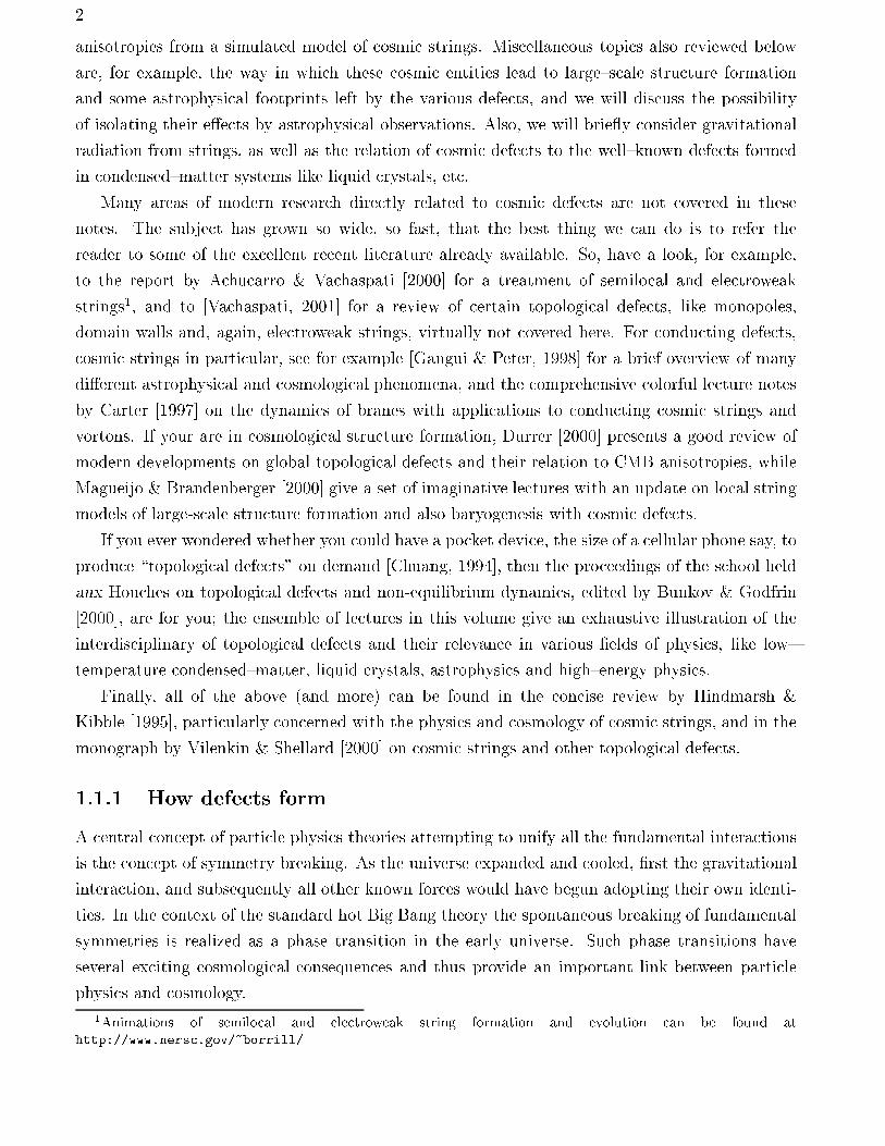
Figure 1.1: Temperaturedependent eective potential for a rstorder phase transition for theHiggs eld. For very high temperatures, well above the critical one Tc, the potential possesses justone minimum for the vanishing value of the Higgs eld. Then, when the temperature decreases,a whole set of minima develops (it may be two or more, discrete or continuous, depending of thetype of symmetry under consideration). Below Tc, the value = 0 stops being the global minimumand the system will spontaneously choose a new (lower) one, say = exp(i) (for complex ) forsome angle and nonvanishing , amongst the available ones. This choice signals the breakdownof the symmetry in a cosmic phase transition and the generation of random regions of con ictingeld orientations . In a cosmological setting, the merging of these domains gives rise to cosmicdefects.

Figure 1.1).

Kibble [1976] rst saw the possibility of defect formation when he realized that in a cooling

universe phase transitions proceed by the formation of uncorrelated domains that subsequently

coalesce, leaving behind relics in the form of defects. In the expanding universe, widely separated

regions in space have not had enough time to `communicate' amongst themselves and are therefore

not correlated, due to a lack of causal contact. It is therefore natural to suppose that dierent

regions ended up having arbitrary orientations of the Higgs eld and that, when they merged

together, it was hard for domains with very dierent preferred directions to adjust themselves and

t smoothly. In the interfaces of these domains, defects form. Such relic ` aws' are unique examples

of incredible amounts of energy and this feature attracted the minds of many cosmologists.

1.1.2 Phase transitions and nite temperature eld theory

Phase transitions are known to occur in the early universe. Examples we mentioned are the quark

to hadron (connement) transition, which QCD predicts at an energy around 1 GeV, and the

electroweak phase transition at about 250 GeV. Within grand unied theories (GUT), aiming to

describe the physics beyond the standard model, other phase transitions are predicted to occur at

energies of order 1015 GeV; during these, the Higgs eld tends to fall towards the minima of its

5

potential while the overall temperature of the universe decreases as a consequence of the expansion.

A familiar theory to make a bit more quantitative the above considerations is the jj4 theory,

L =1

2j@j2 + 1

2m2

0jj2

4!jj4 ; (1.1)

with m20 > 0. The second and third terms on the right hand side yield the usual `Mexican hat'

potential for the complex scalar eld. For energies much larger than the critical temperature, Tc,

the elds are in the socalled `false' vacuum: a highly symmetric state characterized by a vacuum

expectation value hjji = 0. But when energies decrease the symmetry is spontaneously broken:

a new `true' vacuum develops and the scalar eld rolls down the potential and sits onto one of the

degenerate new minima. In this situation the vacuum expectation value becomes hjji2 = 6m20=.

Research done in the 1970's in nitetemperature eld theory [Weinberg, 1974; Dolan & Jackiw,

1974; Kirzhnits & Linde, 1974] has led to the result that the temperaturedependent eective

potential can be written down as

VT (jj) = 12m2(T )jj2 +

4!jj4 (1.2)

with T 2c = 24m2

0=, m2(T ) = m2

0(1 T 2=T 2c ), and hjji2 = 6m2(T )=. We easily see that when T

approaches Tc from below the symmetry is restored, and again we have hjji = 0. In condensed

matter jargon, the transition described above is secondorder [Mermin, 1979].2

1.1.3 The Kibble mechanism

The model described in the last subsection is an example in which the transition may be second

order. As we saw, for temperatures much larger than the critical one the vacuum expectation value

of the scalar eld vanishes at all points of space, whereas for T < Tc it evolves smoothly in time

towards a non vanishing hjji. Both thermal and quantum uctuations in uence the new value

taken by hjji and therefore it has no reasons to be uniform in space. This leads to the existence

of domains wherein the hj(~x)ji is coherent and regions where it is not. The consequences of this

fact are the subject of this subsection.

Phase transitions can also be rstorder proceeding via bubble nucleation. At very high energies

the symmetry breaking potential has hjji = 0 as the only vacuum state. When the temperature

goes down to Tc a set of vacua, degenerate to the previous one, develops. However this time the

transition is not smooth as before, for a potential barrier separates the old (false) and the new

(true) vacua (see, e.g. Figure 1.1). Provided the barrier at this small temperature is high enough,

compared to the thermal energy present in the system, the eld will remain trapped in the

false vacuum state even for small (< Tc) temperatures. Classically, this is the complete picture.

However, quantum tunneling eects can liberate the eld from the old vacuum state, at least in

2In a rstorder phase transition the order parameter (e.g.,jjin our case) is not continuous. It may proceed

by bubble nucleation [Callan & Coleman, 1977; Linde, 1983b] or by spinoidal decomposition [Langer, 1992]. Phasetransitions can also be continuous secondorder processes. The `order' depends sensitively on the ratio of thecoupling constants appearing in the Lagrangian.

6

some regions of space: there is a probability per unit time and volume in space that at a point ~x

a bubble of true vacuum will nucleate. The result is thus the formation of bubbles of true vacuum

with the value of the eld in each bubble being independent of the value of the eld in all other

bubbles. This leads again to the formation of domains where the elds are correlated, whereas no

correlation exits between elds belonging to dierent domains. Then, after creation the bubble

will expand at the speed of light surrounded by a `sea' of false vacuum domains. As opposed

to secondorder phase transitions, here the nucleation process is extremely inhomogeneous and

hj(~x)ji is not a continuous function of time.

Let us turn now to the study of correlation lengths and their role in the formation of topological

defects. One important feature in determining the size of the domains where hj(~x)ji is coherentis given by the spatial correlation of the eld . Simple eld theoretic considerations [see, e.g.,

Copeland, 1993] for long wavelength uctuations of lead to dierent functional behaviors for the

correlation function G(r) h(r1)(r2)i, where we noted r = jr1 r2j. What is found depends

radically on whether the wanted correlation is computed between points in space separated by

a distance r much smaller or much larger than a characteristic length 1 = m(T ) ' p jhij,known as the correlation length. We have

G(r) '8><>:

Tc

4rexp( r

) r >>

T 2

22r << :

(1.3)

This tells us that domains of size m1 arise where the eld is correlated. On the other

hand, well beyond no correlations exist and thus points separated apart by r >> will belong

to domains with in principle arbitrarily dierent orientations of the Higgs eld. This in turn leads,

after the merging of these domains in a cosmological setting, to the existence of defects, where

eld congurations fail to match smoothly.

However, when T ! Tc we have m ! 0 and so ! 1, suggesting perhaps that for all

points of space the eld becomes correlated. This fact clearly violates causality. The existence

of particle horizons in cosmological models (proportional to the inverse of the Hubble parameter

H1) constrains microphysical interactions over distances beyond this causal domain. Therefore

we get an upper bound to the correlation length as < H1 t.

The general feature of the existence of uncorrelated domains has become known as the Kibble

mechanism [Kibble, 1976] and it seems to be generic to most types of phase transitions.

1.1.4 A survey of topological defects

Dierent models for the Higgs eld lead to the formation of a whole variety of topological defects,

with very dierent characteristics and dimensions. Some of the proposed theories have symmetry

breaking patterns leading to the formation of `domain walls' (mirror re ection discrete symmetry):

incredibly thin planar surfaces trapping enormous concentrations of massenergy which separate

domains of con icting eld orientations, similar to twodimensional sheetlike structures found

7

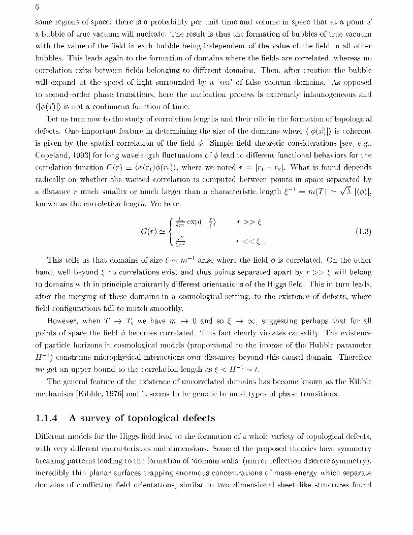
Figure 1.2: In a simple model of symmetry breaking, the initial symmetric ground state of theHiggs eld (yellow dot) can fall into the left- or right-hand valley of a double-well energy potential(light and dark dots). In a cosmic phase transition, regions of the new phase appear randomlyand begin to grow and eventually merge as the transition proceeds toward completion (middle).Regions in which the symmetry has broken the same way can coalesce, but where regions thathave made opposite choices encounter each other, a topological defect known as a domain wallforms (right). Across the wall, the Higgs eld has to go from one of the valleys to the other (inthe left panel), and must therefore traverse the energy peak. This creates a narrow planar regionof very high energy, in which the symmetry is locally unbroken.

in ferromagnets. Within other theories, cosmological elds get distributed in such a way that

the old (symmetric) phase gets conned into a nite region of space surrounded completely by

the new (nonsymmetric) phase. This situation leads to the generation of defects with linear

geometry called `cosmic strings'. Theoretical reasons suggest these strings (vortex lines) do not

have any loose ends in order that the two phases not get mixed up. This leaves innite strings

and closed loops as the only possible alternatives for these defects to manifest themselves in the

early universe3.

With a bit more abstraction scientists have even conceived other (semi) topological defects,

called `textures'. These are conceptually simple objects, yet, it is not so easy to imagine them for

they are just global eld congurations living on a threesphere vacuum manifold (the minima

of the eective potential energy), whose non linear evolution perturbs spacetime. Turok [1989]

was the rst to realize that many unied theories predicted the existence of peculiar Higgs eld

congurations known as (texture) knots, and that these could be of potential interest for cosmology.

Several features make these defects interesting. In contrast to domain walls and cosmic strings,

textures have no core and thus the energy is more evenly distributed over space. Secondly, they are

unstable to collapse and it is precisely this last feature which makes these objects cosmologically

relevant, for this instability makes texture knots shrink to a microscopic size, unwind and radiate

3`Monopole' is another possible topological defect; we defer its discussion to the next subsection. Cosmic stringsbounded by monopoles is yet another possibility in GUT phase transitions of the kind, e.g., G! K U(1)! K.The rst transition yields monopoles carrying a magnetic charge of the U(1) gauge eld, while in the secondtransition the magnetic eld in squeezed into ux tubes connecting monopoles and antimonopoles [Langacker & Pi,1980].

8

away all their energy. In so doing, they generate a gravitational eld that perturbs the surrounding

matter in a way which can seed structure formation.

1.1.5 Conditions for their existence: topological criteria

Let us now explore the conditions for the existence of topological defects. It is widely accepted that

the nal goal of particle physics is to provide a unied gauge theory comprising strong, weak and

electromagnetic interactions (and some day also gravitation). This unied theory is to describe

the physics at very high temperatures, when the age of the universe was slightly bigger than

the Planck time. At this stage, the universe was in a state with the highest possible symmetry,

described by a symmetry groupG, and the Lagrangian modeling the system of all possible particles

and interactions present should be invariant under the action of the elements of G.

As we explained before, the form of the nite temperature eective potential of the system is

subject to variations during the cooling down evolution of the universe. This leads to a chain of

phase transitions whereby some of the symmetries present in the beginning are not present anymore

at lower temperatures. The rst of these transitions may be described as G!H, where now H

stands for the new (smaller) unbroken symmetry group ruling the system. This chain of symmetry

breakdowns eventually ends up with SU(3)SU(2)U(1), the symmetry group underlying the

`standard model' of particle physics.

A broken symmetry system (with a Mexican-hat potential for the Higgs eld) may have many

dierent minima (with the same energy), all related by the underlying symmetry. Passing from

one minimum to another is included as one of the symmetries of the original group G, and the

system will not change due to one such transformation. If a certain eld conguration yields the

lowest energy state of the system, transformations of this conguration by the elements of the

symmetry group will also give the lowest energy state. For example, if a spherically symmetric

system has a certain lowest energy value, this value will not change if the system is rotated.

The system will try to minimize its energy and will spontaneously choose one amongst the

available minima. Once this is done and the phase transition achieved, the system is no longer

ruled by G but by the symmetries of the smaller group H. So, if G!H and the system is in one

of the lowest energy states (call it S1), transformations of S1 to S2 by elements of G will leave the

energy unchanged. However, transformations of S1 by elements of H will leave S1 itself (and not

just the energy) unchanged. The many distinct ground states of the system S1; S2; : : : are given

by all transformations of G that are not related by elements in H. This space of distinct ground

states is called the vacuum manifold and denotedM.

M is the space of all elements of G in which elements related by transformations in H

have been identied. Mathematicians call it the coset space and denote it G=H. We

then haveM = G=H.

The importance of the study of the vacuum manifold lies in the fact that it is precisely the

topology ofM what determines the type of defect that will arise. Homotopy theory tells us how

9

to mapM into physical space in a nontrivial way, and what ensuing defect will be produced. For

instance, the existence of non contractible loops inM is the requisite for the formation of cosmic

strings. In formal language this comes about whenever we have the rst homotopy group 1(M) 6=1, where 1 corresponds to the trivial group. If the vacuum manifold is disconnected we then have

0(M) 6= 1, and domain walls are predicted to form in the boundary of these regions where the

eld is away from the minimum of the potential. Analogously, if 2(M) 6= 1 it follows that the

vacuum manifold contains non contractible twospheres, and the ensuing defect is a monopole.

Textures arise when M contains non contractible threespheres and in this case it is the third

homotopy group, 3(M), the one that is non trivial. We summarize this in Table 1.1 .

0(M) 6=1 M disconnected Domain Walls

1(M) 6=1 non contractible loops inM Cosmic Strings

2(M) 6=1 non contractible 2spheres inM Monopoles

3(M) 6=1 non contractible 3spheres inM Textures

Table 1.1: The topology ofM determines the type of defect that will arise.

1.2 Defects in the universe

Generically topological defects will be produced if the conditions for their existence are met. Then

for example if the unbroken group H contains a disconnected part, like an explicit U(1) factor

(something that is quite common in many phase transition schemes discussed in the literature),

monopoles will be left as relics of the transition. This is due to the fundamental theorem on the

second homotopy group of coset spaces [Mermin, 1979], which states that for a simplyconnected

covering group G we have4

2(G=H) = 1(H0) ; (1.4)

with H0 being the component of the unbroken group connected to the identity. Then we see that

since monopoles are associated with unshrinkable surfaces in G=H, the previous equation implies

their existence if H is multiplyconnected. The reader may guess what the consequences are for

GUT phase transitions: in grand unied theories a semisimple gauge group G is broken in several

stages down to H = SU(3)U(1). Since in this case 1(H) = Z, the integers, we have 2(G=H) 6=1 and therefore gauge monopole solutions exist [Preskill, 1979].

4The isomorsm between two groups is noted as =. Note that by using the theorem we therefore can reducethe computation of 2 for a coset space to the computation of 1 for a group. A word of warning: the focus here ison the physics and the mathematicallyoriented reader should bear this in mind, especially when we will become abit sloppy with the notation. In case this happens, consult the book [Steenrod, 1951] for a clear exposition of thesematters.

10

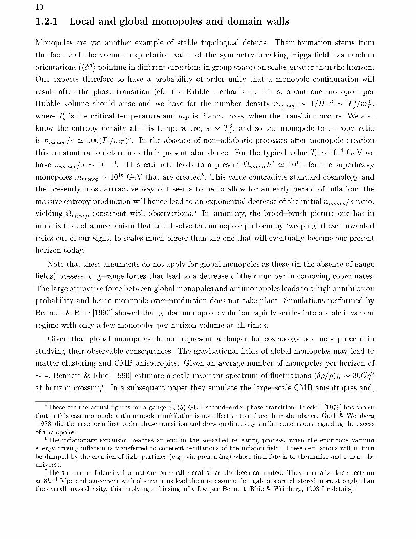
1.2.1 Local and global monopoles and domain walls

Monopoles are yet another example of stable topological defects. Their formation stems from

the fact that the vacuum expectation value of the symmetry breaking Higgs eld has random

orientations (hai pointing in dierent directions in group space) on scales greater than the horizon.One expects therefore to have a probability of order unity that a monopole conguration will

result after the phase transition (cf. the Kibble mechanism). Thus, about one monopole per

Hubble volume should arise and we have for the number density nmonop 1=H3 T 6c =m

3P ,

where Tc is the critical temperature and mP is Planck mass, when the transition occurs. We also

know the entropy density at this temperature, s T 3c , and so the monopole to entropy ratio

is nmonop=s ' 100(Tc=mP )3. In the absence of nonadiabatic processes after monopole creation

this constant ratio determines their present abundance. For the typical value Tc 1014 GeV we

have nmonop=s 1013. This estimate leads to a present monoph2 ' 1011, for the superheavy

monopoles mmonop ' 1016 GeV that are created5. This value contradicts standard cosmology and

the presently most attractive way out seems to be to allow for an early period of in ation: the

massive entropy production will hence lead to an exponential decrease of the initial nmonop=s ratio,

yielding monop consistent with observations.6 In summary, the broadbrush picture one has in

mind is that of a mechanism that could solve the monopole problem by `weeping' these unwanted

relics out of our sight, to scales much bigger than the one that will eventually become our present

horizon today.

Note that these arguments do not apply for global monopoles as these (in the absence of gauge

elds) possess longrange forces that lead to a decrease of their number in comoving coordinates.

The large attractive force between global monopoles and antimonopoles leads to a high annihilation

probability and hence monopole overproduction does not take place. Simulations performed by

Bennett & Rhie [1990] showed that global monopole evolution rapidly settles into a scale invariant

regime with only a few monopoles per horizon volume at all times.

Given that global monopoles do not represent a danger for cosmology one may proceed in

studying their observable consequences. The gravitational elds of global monopoles may lead to

matter clustering and CMB anisotropies. Given an average number of monopoles per horizon of

4, Bennett & Rhie [1990] estimate a scale invariant spectrum of uctuations (Æ=)H 30G2

at horizon crossing7. In a subsequent paper they simulate the largescale CMB anisotropies and,

5These are the actual gures for a gauge SU(5) GUT secondorder phase transition. Preskill [1979] has shownthat in this case monopole antimonopole annihilation is not eective to reduce their abundance. Guth & Weinberg[1983] did the case for a rstorder phase transition and drew qualitatively similar conclusions regarding the excessof monopoles.

6The in ationary expansion reaches an end in the socalled reheating process, when the enormous vacuumenergy driving in ation is transferred to coherent oscillations of the in aton eld. These oscillations will in turnbe damped by the creation of light particles (e.g., via preheating) whose nal fate is to thermalise and reheat theuniverse.

7The spectrum of density uctuations on smaller scales has also been computed. They normalize the spectrumat 8h1 Mpc and agreement with observations lead them to assume that galaxies are clustered more strongly thanthe overall mass density, this implying a `biasing' of a few [see Bennett, Rhie & Weinberg, 1993 for details].

11

upon normalization with COBEDMR, they get roughly G2 6 107 in agreement with a

GUT energy scale [Bennett & Rhie, 1993]. However, as we will see in the CMB sections below,

current estimates for the angular power spectrum of global defects do not match the most recent

observations, their main problem being the lack of power on the degree angular scale once the

spectrum is normalized to COBE on large scales.

Let us concentrate now on domain walls, and brie y try to show why they are not welcome in

any cosmological context (at least in the simple version we here consider there is always room

for more complicated (and contrived) models). If the symmetry breaking pattern is appropriate

at least one domain wall per horizon volume will be formed. The mass per unit surface of these

two-dimensional objects is given by 1=23, where as usual is the coupling constant in the

symmetry breaking potential for the Higgs eld. Domain walls are generally horizonsized and

therefore their mass is given by 1=23H2. This implies a mass energy density roughly given

by DW 3t1 and we may readily see now how the problem arises: the critical density goes

as crit t2 which implies DW (t) (=mP )2t. Taking a typical GUT value for we get

DW (t 1035sec) 1 already at the time of the phase transition. It is not hard to imagine that

today this will be at variance with observations; in fact we get DW (t 1018sec) 1052. This

indicates that models where domain walls are produced are tightly constrained, and the general

feeling is that it is best to avoid them altogether [see Kolb & Turner, 1990 for further details; see

also Dvali et al., 1998, Pogosian & Vachaspati, 2000 8 and Alexander et al., 1999 for an alternative

solution].

1.2.2 Are defects in ated away?

It is important to realize the relevance that the Kibble's mechanism has for cosmology; nearly every

sensible grand unied theory (with its own symmetry breaking pattern) predicts the existence of

defects. We know that an early era of in ation helps in getting rid of the unwanted relics. One

could well wonder if the very same Higgs eld responsible for breaking the symmetry would not

be the same one responsible for driving an era of in ation, thereby diluting the density of the

relic defects. This would get rid not only of (the unwanted) monopoles and domain walls but also

of any other (cosmologically appealing) defect. Let us follow [Brandenberger, 1993] and sketch

why this actually does not occur. Take rst the symmetry breaking potential of Eq. (1.2) at

zero temperature and add to it a harmless independent term 3m4=(2). This will not aect the

dynamics at all. Then we are led to

V () =

4!

2 2

2; (1.5)

8Animations of monopoles colliding with domain walls can be found in `LEP' page athttp://theory.ic.ac.uk/~LEP/figures.html

12

with = (6m2=)1=2 the symmetry breaking energy scale, and where for the present heuristic

digression we just took a real Higgs eld. Consider now the equation of motion for ,

' @V@

= 3!3 +m2 m2 ; (1.6)

for << very near the false vacuum of the eective Mexican hat potential and where, for sim-

plicity, the expansion of the universe and possible interactions of with other elds were neglected.

The typical time scale of the solution is ' m1. For an in ationary epoch to be eective we

need >> H1, i.e., a suÆciently large number of efolds of slowrolling solution. Note, however,

that after some efolds of exponential expansion the curvature term in the Friedmann equation

becomes subdominant and we have H2 ' 8G V (0)=3 ' (2m2=3)(=mP )2. So, unless > mP ,

which seems unlikely for a GUT phase transition, we are led to << H1 and therefore the

amount of in ation is not enough for getting rid of the defects generated during the transition by

hiding them well beyond our present horizon.

Recently, there has been a large amount of work in getting defects, particularly cosmic strings,

after post-in ationary preheating. Reaching the latest stages of the in ationary phase, the in aton

eld oscillates about the minimum of its potential. In doing so, parametric resonance may transfer

a huge amount of energy to other elds leading to cosmologically interesting nonthermal phase

transitions. Just like thermal uctuations can restore broken symmetries, here also, these large

uctuations may lead to the whole process of defect formation again. Numerical simulations

employing potentials similar to that of Eq. (1.5) have shown that strings indeed arise for values

1016 GeV [Tkachev et al., 1998, Kasuya & Kawasaki, 1998]. Hence, preheating after in ation

helps in generating cosmic defects.

1.2.3 Cosmic strings

Cosmic strings are without any doubt the topological defect most thoroughly studied, both in

cosmology and solidstate physics (vortices). The canonical example, also describing ux tubes in

superconductors, is given by the Lagrangian

L = 14FF

+1

2jDj2

4!

jj2 2

2; (1.7)

with F = @[A], where A is the gauge eld and the covariant derivative is D = @ + ieA,

with e the gauge coupling constant. This Lagrangian is invariant under the action of the Abelian

group G = U(1), and the spontaneous breakdown of the symmetry leads to a vacuum manifoldMthat is a circle, S1, i.e., the potential is minimized for = exp(i), with arbitrary 0 2.

Each possible value of corresponds to a particular `direction' in the eld space.

Now, as we have seen earlier, due to the overall cooling down of the universe, there will be

regions where the scalar eld rolls down to dierent vacuum states. The choice of the vacuum is

totally independent for regions separated apart by one correlation length or more, thus leading to

the formation of domains of size 1. When these domains coalesce they give rise to edges in

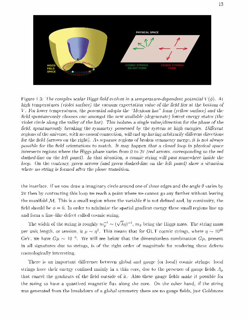
13

HIGGS FIELDSPACE

PHYSICAL SPACE

COSMIC STRINGS DO NOT FORM

COSMIC STRINGSFORM

Figure 1.3: The complex scalar Higgs eld evolves in a temperature-dependent potential V (). Athigh temperatures (violet surface) the vacuum expectation value of the eld lies at the bottom ofV . For lower temperatures, the potential adopts the \Mexican hat" form (yellow surface) and theeld spontaneously chooses one amongst the new available (degenerate) lowest energy states (theviolet circle along the valley of the hat). This isolates a single value/direction for the phase of theeld, spontaneously breaking the symmetry possessed by the system at high energies. Dierentregions of the universe, with no causal connection, will end up having arbitrarily dierent directionsfor the eld (arrows on the right). As separate regions of broken symmetry merge, it is not alwayspossible for the eld orientations to match. It may happen that a closed loop in physical spaceintersects regions where the Higgs phase varies from 0 to 2 (red arrows, corresponding to the reddashed-line on the left panel). In that situation, a cosmic string will pass somewhere inside theloop. On the contrary, green arrows (and green dashed-line on the left panel) show a situationwhere no string is formed after the phase transition.

the interface. If we now draw a imaginary circle around one of these edges and the angle varies by

2 then by contracting this loop we reach a point where we cannot go any further without leaving

the manifoldM. This is a small region where the variable is not dened and, by continuity, the

eld should be = 0. In order to minimize the spatial gradient energy these small regions line up

and form a linelike defect called cosmic string.

The width of the string is roughly m1 (

p)1, m being the Higgs mass. The string mass

per unit length, or tension, is 2. This means that for GUT cosmic strings, where 1016

GeV, we have G 106. We will see below that the dimensionless combination G, present

in all signatures due to strings, is of the right order of magnitude for rendering these defects

cosmologically interesting.

There is an important dierence between global and gauge (or local) cosmic strings: local

strings have their energy conned mainly in a thin core, due to the presence of gauge elds A

that cancel the gradients of the eld outside of it. Also these gauge elds make it possible for

the string to have a quantized magnetic ux along the core. On the other hand, if the string

was generated from the breakdown of a global symmetry there are no gauge elds, just Goldstone

14

PHYSICAL SPACE3 - DIMENSIONAL PHYSICAL SPACE

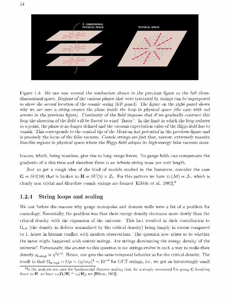
Figure 1.4: We can now extend the mechanism shown in the previous gure to the full three-dimensional space. Regions of the various planes that were traversed by strings can be superposedto show the actual location of the cosmic string (left panel). The gure on the right panel showswhy we are sure a string crosses the plane inside the loop in physical space (the case with redarrows in the previous gure). Continuity of the eld imposes that if we gradually contract thisloop the direction of the eld will be forced to wind \faster". In the limit in which the loop reducesto a point, the phase is no longer dened and the vacuum expectation value of the Higgs eld has tovanish. This corresponds to the central tip of the Mexican hat potential in the previous gure andis precisely the locus of the false vacuum. Cosmic strings are just that, narrow, extremely massiveline-like regions in physical space where the Higgs eld adopts its high-energy false vacuum state.

bosons, which, being massless, give rise to longrange forces. No gauge elds can compensate the

gradients of this time and therefore there is an innite string mass per unit length.

Just to get a rough idea of the kind of models studied in the literature, consider the case

G = SO(10) that is broken to H = SU(5) Z2. For this pattern we have 1(M) = Z2, which is

clearly non trivial and therefore cosmic strings are formed [Kibble et al., 1982].9

1.2.4 String loops and scaling

We saw before the reasons why gauge monopoles and domain walls were a bit of a problem for

cosmology. Essentially, the problem was that their energy density decreases more slowly than the

critical density with the expansion of the universe. This fact resulted in their contribution to

def (the density in defects normalized by the critical density) being largely in excess compared

to 1, hence in blatant con ict with modern observations. The question now arises as to whether

the same might happened with cosmic strings. Are strings dominating the energy density of the

universe? Fortunately, the answer to this question is no; strings evolve in such a way to make their

density strings / 2t2. Hence, one gets the same temporal behavior as for the critical density. The

result is that strings G (=mP )2 106 for GUT strings, i.e., we get an interestingly small

9In the analysis one uses the fundamental theorem stating that, for a simplyconnected Lie group G breakingdown to H, we have 1(G=H) = 0(H); see [Hilton, 1953].

15

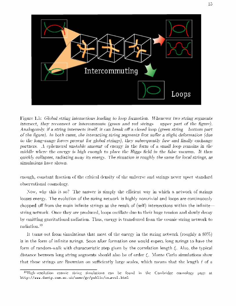
Figure 1.5: Global string interactions leading to loop formation. Whenever two string segmentsintersect, they reconnect or intercommute (green and red strings upper part of the gure).Analogously, if a string intersects itself, it can break o a closed loop (green string bottom partof the gure). In both cases, the interacting string segments rst suer a slight deformation (dueto the longrange forces present for global strings), they subsequently fuse and nally exchangepartners. A ephemeral unstable amount of energy in the form of a small loop remains in themiddle where the energy is high enough to place the Higgs eld in the false vacuum. It thenquickly collapses, radiating away its energy. The situation is roughly the same for local strings, assimulations have shown.

enough, constant fraction of the critical density of the universe and strings never upset standard

observational cosmology.

Now, why this is so? The answer is simply the eÆcient way in which a network of strings

looses energy. The evolution of the string network is highly nontrivial and loops are continuously

chopped o from the main innite strings as the result of (self) intersections within the innite

string network. Once they are produced, loops oscillate due to their huge tension and slowly decay

by emitting gravitational radiation. Thus, energy is transferred from the cosmic string network to

radiation.10

It turns out from simulations that most of the energy in the string network (roughly a 80%)

is in the form of innite strings. Soon after formation one would expect long strings to have the

form of random-walk with characteristic step given by the correlation length . Also, the typical

distance between long string segments should also be of order . Monte Carlo simulations show

that these strings are Brownian on suÆciently large scales, which means that the length ` of a

10Highresolution cosmic string simulations can be found in the Cambridge cosmology page athttp://www.damtp.cam.ac.uk/user/gr/public/cs evol.html

16

string is related to the end-to-end distance d of two given points along the string (with d ) in

the form

` = d2=: (1.8)

What remains of the energy is given in the form of closed loops with no preferred length scale (a

scale invariant distribution) which implies that the number density of loops having sizes between

R and R + dR follows just from dimensional analysis

dnloops / dR

R4(1.9)

which is just another way of saying that nloops / 1=R3, loops behave like normal nonrelativistic

matter. The actual coeÆcient, as usual, comes from string simulations.

There are both analytical and numerical indications in favor of the existence of a stable \scaling

solution" for the cosmic string network. After generation, the network quickly evolves in a self

similar manner with just a few innite string segments per Hubble volume and Hubble time. A

heuristic argument for the scaling solution due to Vilenkin [1985] is as follows.

If we take (t) to be the mean number of innite string segments per Hubble volume, then the

energy density in innite strings strings = s is

s(t) = (t)2t2 = (t)t2: (1.10)

Now, strings will typically have intersections, and so the number of loops nloops(t) = nl(t)

produced per unit volume will be proportional to 2. We nd

dnl 2R4dR: (1.11)

Hence, recalling now that the loop sizes grow with the expansion like R / t we have

dnl(t)

dt p2t4 (1.12)

where p is the probability of loop formation per intersection, a quantity related to the intercommut-

ing probability, both roughly of order 1. We are now in a position to write an energy conservation

equation for strings plus loops in the expanding universe. Here it is

dsdt

+3

2ts ml

dnldt tdnl

dt(1.13)

where ml = t is just the loop mass and where the second on the left hand side is the dilution term

3Hs for an expanding radiationdominated universe. The term on the right hand side amounts to

the loss of energy from the long string network by the generation of small closed loops. Plugging

Eqs. (1.10) and (1.12) into (1.13) Vilenkin nds the following kinetic equation for (t)

d

dt

2t p

2

t(1.14)

with p 1. Thus if 1 then d=dt < 0 and tends to decrease in time, while if 1 then

d=dt > 0 and increases. Hence, there will be a stable solution with a few.

17

1.2.5 Global textures

Whenever a global nonAbelian symmetry is spontaneously and completely broken (e.g. at a

grand unication scale), global defects called textures are generated. Theories where this global

symmetry is only partially broken do not lead to global textures, but instead to global monopoles

and nontopological textures. As we already mentioned global monopoles do not suer the same

constraints as their gauge counterparts: essentially, having no associated gauge elds, the long

range forces between pairs of monopoles lead to the annihilation of their eventual excess and as

a result monopoles scale with the expansion. On the other hand, nontopological textures are

a generalization that allows the broken subgroup H to contain nonAbelian factors. It is then

possible to have 3 trivial as in, e.g., SO(5)!SO(4) broken by a vector, for which case we have

M = S4, the foursphere [Turok, 1989]. Having explained this, let us concentrate in global

topological textures from now on.

Textures, unlike monopoles or cosmic strings, are not well localized in space. This is due to the

fact that the eld remains in the vacuum everywhere, in contrast to what happens for other defects,

where the eld leaves the vacuum manifold precisely where the defect core is. Since textures do

not possess a core, all the energy of the eld conguration is in the form of eld gradients. This

fact is what makes them interesting objects only when coming from global theories: the presence

of gauge elds A could (by a suitable reorientation) compensate the gradients of and yield

D = 0, hence canceling out (gauging away) the energy of the conguration11.

One feature endowed by textures that really makes these defects peculiar is their being unstable

to collapse. The initial eld conguration is set at the phase transition, when develops a nonzero

vacuum expectation value. lives in the vacuum manifoldM and winds around M in a non

trivial way on scales greater than the correlation length, < t. The evolution is determined by the

nonlinear dynamics of . When the typical size of the defect becomes of the order of the horizon,

it collapses on itself. The collapse continues until eventually the size of the defect becomes of the

order of 1, and at that point the energy in gradients is large enough to raise the eld from its

vacuum state. This makes the defect unwind, leaving behind a trivial eld conguration. As a

result grows to about the horizon scale, and then keeps growing with it. As still larger scales come

across the horizon, knots are constantly formed, since the eld points in dierent directions onMin dierent Hubble volumes. This is the scaling regime for textures, and when it holds simulations

show that one should expect to nd of order 0.04 unwinding collapses per horizon volume per

Hubble time [Turok, 1989]. However, unwinding events are not the most frequent feature [Borrill

et al., 1994], and when one considers random eld congurations without an unwinding event the

number raises to about 1 collapse per horizon volume per Hubble time.

11This does not imply, however, that the classical dynamics of a gauge texture is trivial. The evolution ofthe A system will be determined by the competing tendencies of the global eld to unwind and of the gaugeeld to compensate the gradients. The result depends on the characteristic size L of the texture: in the rangem1 << L << m1A (e)1 the behavior of the gauge texture resembles that of the global texture, as it should,

since in the limit mA very small (e! 0) the gauge texture turns into a global one [Turok & Zadrozny, 1990].

18

1.2.6 Evolution of global textures

We mentioned earlier that the breakdown of any nonAbelian global symmetry led to the formation

of textures. The simplest possible example involves the breakdown of a global SU(2) by a complex

doublet a, where the latter may be expressed as a fourcomponent scalar eld, i.e., a = 1 : : : 4.

We may write the Lagrangian of the theory much in the same way as it was done in Eq. (1.7),

but now we drop the gauge elds (thus the covariant derivatives become partial derivatives). Let

us take the symmetry breaking potential as follows, V () = 4(jj2 2)2. The situation in which

a global SU(2) in broken by a complex doublet with this potential V is equivalent to the theory

where SO(4) is broken by a fourcomponent vector to SO(3), by making a take on a vacuum

expectation value. We then have the vacuum manifoldM given by SO(4)/SO(3) = S3, namely, a

threesphere with aa = 2. As 3(S3) 6= 1 (in fact, 3(S

3) = Z) we see we will have nontrivialsolutions of the eld a and global textures will arise.

As usual, variation of the action with respect to the eld a yields the equation of motion

b00+ 2

a0

ab

0 r2b = a2 @V@b

; (1.15)

where primes denote derivatives with respect to conformal time and r is computed in comoving

coordinates. When the symmetry in broken three of the initially four degrees of freedom go into

massless Goldstone bosons associated with the three directions tangential to the vacuum three

sphere. The `radial' massive mode that remains (m p) will not be excited, provided we

concentrate on length scales much larger than m1 .

To solve for the dynamics of the eld b, two dierent approaches have been implemented in the

literature. The rst one faces directly the full equation (1.15), trying to solve it numerically. The

alternative to this exploits the fact that, at temperatures smaller than Tc, the eld is constrained

to live in the true vacuum. By implementing this fact via a Lagrange multiplier12 we get

rrb = r

crc2

b ; 2 = 2 ; (1.16)

with r the covariant derivative operator. Eq. (1.16) represents a nonlinear sigma model for the

interaction of the three massless modes [Rajaraman, 1982]. This last approach is only valid when

probing length scales larger than the inverse of the mass m1 . As we mentioned before, when

this condition is not met the gradients of the eld are strong enough to make it leave the vacuum

manifold and unwind.

The approach (cf. Eqs. (1.16)) is suitable for analytic inspection. In fact, an exact at space

solution was found assuming a spherically symmetric ansatz. This solution represents the collapse

and subsequent conversion of a texture knot into massless Goldstone bosons, and is known as the

spherically symmetric selfsimilar (SSSS) exact unwinding solution. We will say no more here

with regard to the this solution, but just refer the interested reader to the original articles [see,

12In fact, in the action the coupling constant of the `Mexican hat' potential is interpreted as the Lagrangemultiplier.

19

e.g., Turok & Spergel, 1990; Notzold, 1991]. Simulations taking full account of the energy stored

in gradients of the eld, and not just in the unwinding events, like in Eq. (1.15), were performed,

for example, in [Durrer & Zhou, 1995]. 13

1.3 Currents along strings

In the past few years it has become clear that topological defects, and in particular strings, will be

endowed with a considerably richer structure than previously envisaged. In generic grand unied

models the Higgs eld, responsible for the existence of cosmic strings, will have interactions with

other fundamental elds. This should not surprise us, for well understood low energy particle

theories include eld interactions in order to account for the well measured masses of light fermions,

like the familiar electron, and for the masses of gauge bosons W and Z discovered at CERN in

the eighties. Thus, when one of these fundamental (electromagnetically charged) elds present in

the model condenses in the interior space of the string, there will appear electric currents owing

along the string core.

Even though these strings are the most attractive ones, the fact of them having electromagnetic

properties is not actually fundamental for understanding the dynamics of circular string loops. In

fact, while in the uncharged and non current-carrying case symmetry arguments do not allow

us to distinguish the existence of rigid rotations around the loop axis, the very existence of a

small current breaks this symmetry, marking a denite direction, which allows the whole loop

conguration to rotate. This can also be viewed as the existence of spinning particlelike solutions

trapped inside the core. The stationary loop solutions where the string tension gets balanced by

the angular momentum of the charges is what Davis and Shellard [1988] dubbed vortons.

Vorton congurations do not radiate classically. Because they have loop shapes, implying

periodic boundary conditions on the charged elds, it is not surprising that these congurations

are quantized. At large distances these vortons look like point masses with quantized electric charge

(actually they can have more than a hundred times the electron charge) and angular momentum.

They are very much like particles, hence their name. They are however very peculiar, for their

characteristic size is of order of their charge number (around a hundred) times their thickness,

which is essentially some fourteen orders of magnitude smaller than the classical electron radius.

Also, their mass is often of the order of the energies of grand unication, and hence vortons would

be some twenty orders of magnitude heavier than the electron.

But why should strings become conducting in the rst place? The physics inside the core of the

string diers somewhat from outside of it. In particular the existence of interactions among the

Higgs eld forming the string and other fundamental elds, like that of charged fermions, would

make the latter loose their masses inside the core. Then, only small energies would be required

to produce pairs of trapped fermions and, being eectively massless inside the string core, they

would propagate at the speed of light. These zero energy fermionic states, also called zero modes,

13Simulations of the collapse of `exotic' textures can be found at http://camelot.mssm.edu/~ats/texture.html

20

endow the string with currents and in the case of closed loops they provide the mechanical angular

momentum support necessary for stabilizing the contracting loop against collapse.

1.3.1 GotoNambu Strings

Our aim now is to introduce extra elds into the problem. The simple Lagrangian we saw in

previous sections was a good approximation for ideal structureless strings, known under the name

of GotoNambu strings [Goto, 1971; Nambu, 1970]. Additional elds coupled with the string

forming Higgs eld often lead to interesting eects in the form of generalized currents owing

along the string core.

But before taking into full consideration the internal structure of strings we will start by setting

the scene with the simple Abelian Higgs model (which describes scalar electrodynamics) in order

to x the notation etc. This is a prototype of gauge eld theory with spontaneous symmetry

breaking G = U(1) ! f1g. The Lagrangian reads [Higgs, 1964]

LH= 1

2[D][D]

1

4(F ()

)2

8(jj2 2)2; (1.17)

with gauge covariant derivative D = @ + iqA() , antisymmetric tensor F ()

= rA() rA

()

for the gauge vector eld A() , and complex scalar eld = jjei with gauge coupling q.

The rst solutions for this theory were found by Nielsen & Olesen [1973]. A couple of relevant

properties are noteworthy:

the mass per unit length for the string is = U 2. For GUT local strings this gives

1022g=cm, while one nds 2 ln(r=m1s ) ! 1 if strings are global, due to the

absence of compensating gauge elds. This divergence is in general not an issue, because

global strings only in few instances are isolated; in a string network, a natural cuto is the

distance to the neighboring string.

There are essentially two characteristic mass scales (or inverse length scales) in the problem:

ms 1=2 and mv q, corresponding to the inverse of the Compton wavelengths of the

scalar (Higgs) and vector (A() ) particles, respectively.

There exists a sort of screening of the energy, called `Higgs screening', implying a nite

energy conguration, thanks to the way in which the vector eld behaves far from the string

core: A ! (1=qr)d=d ; for r !1.

After a closed path around the vortex one has (2) = (0), which implies that the winding

phase should be an integer times the cylindrical angle , namely = n. This integer n is

dubbed the `winding number'. In turn, from this fact it follows that there exists a tube of

quantized `magnetic' ux, given by

B=I~A: ~d` =

1

q

Z 2

0

d

dd =

2n

q(1.18)

21

-5

0

5

-5

0

5

0

0.2

0.4

0.6

0.8

1

xy

f(r)

-5

0

5

-5

0

5

0

0.5

1

1.5

2

2.5

Ene

rgy

dens

ity

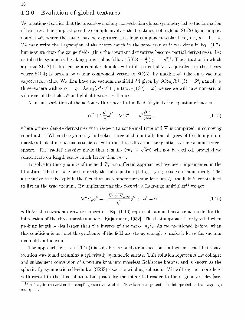
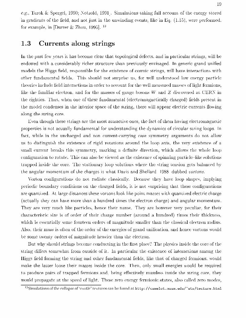
Figure 1.6: Higgs eld and energy proles for GotoNambu cosmic strings. The left panel showsthe amplitude of the Higgs eld around the string. The eld vanishes at the origin (the falsevacuum) and attains its asymptotic value (normalized to unity in the gure) far away from theorigin. The phase of the scalar eld (changing from 0 to 2) is shown by the shading of the surface.In the right panel we show the energy density of the conguration. The maximum value is reachedat the origin, exactly where the Higgs is placed in the false vacuum. [Hindmarsh & Kibble, 1995].

In the string there is a sort of competing eect between the elds: the gauge eld acts in a

repulsive manner; the ux doesn't like to be conned to the core and B lines repel each other. On

the other hand, the scalar eld behaves in an attractive way; it tries to minimize the area where

V () 6= 0, that is, where the eld departs from the true vacuum.

Finally, we can mention a few condensedmatter `cousins' of GotoNambu strings: ux tubes in

superconductors [Abrikosov, 1957] for the nonrelativistic version of gauge strings ( corresponds

to the Cooper pair wave function). Also, vortices in super uids, for the nonrelativistic version

of global strings ( corresponds to the Bose condensate wave function). Moreover, the only two

relevant scales of the problem we mentioned above are the Higgs mass ms and the gauge vector

mass mv. Their inverse give an idea of the characteristic scales on which the elds acquire their

asymptotic solutions far away from the string `location'. In fact, the relevant core widths of the

string are given by m1s and m1

v . It is the comparison of these scales that draws the dividing line

between two qualitatively dierent types of solutions. If we dene the parameter = (ms=mv)2,

superconductivity theory says that < 1 corresponds to Type I behavior while > 1 corresponds

to Type II. For us, < 1 implies that the characteristic scale for the vector eld is smaller than

that for the Higgs eld and so magnetic eld B ux lines are well conned in the core; eventually,

an nvortex string with high winding number n stays stable. On the contrary, > 1 says that the

characteristic scale for the vector eld exceeds that for the scalar eld and thus B ux lines are

not conned; the nvortex string will eventually split into n vortices of ux 2=q. In summary:

= (ms

mv)2< 1 nvortex stable (B ux lines conned in core) Type I> 1 Unstable : splitting into n vortices of ux 2=q Type II

(1.19)

22

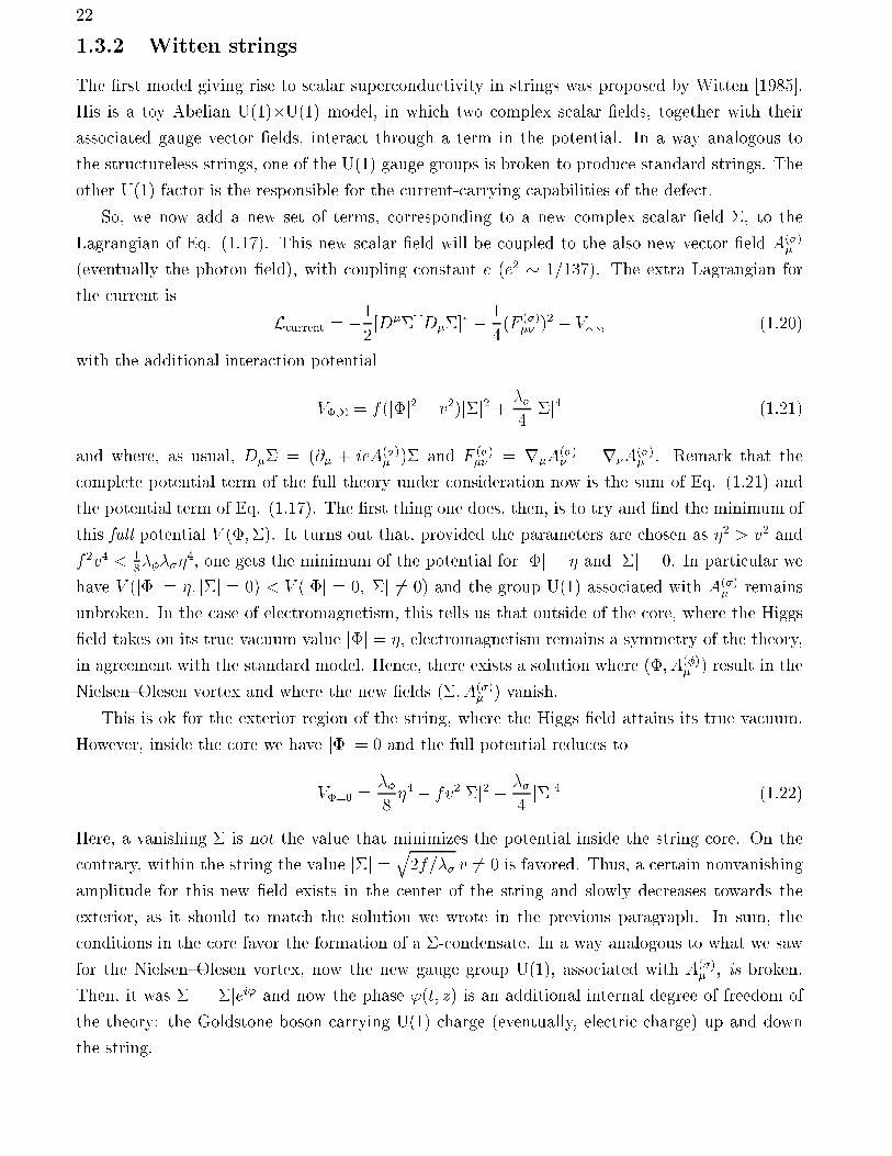
1.3.2 Witten strings

The rst model giving rise to scalar superconductivity in strings was proposed by Witten [1985].

His is a toy Abelian U(1)U(1) model, in which two complex scalar elds, together with their

associated gauge vector elds, interact through a term in the potential. In a way analogous to

the structureless strings, one of the U(1) gauge groups is broken to produce standard strings. The

other U(1) factor is the responsible for the current-carrying capabilities of the defect.

So, we now add a new set of terms, corresponding to a new complex scalar eld , to the

Lagrangian of Eq. (1.17). This new scalar eld will be coupled to the also new vector eld A()

(eventually the photon eld), with coupling constant e (e2 1=137). The extra Lagrangian for

the current is

Lcurrent = 12[D][D]

1

4(F ()

)2 V

;(1.20)

with the additional interaction potential

V; = f(jj2 v2)jj2 + 4jj4 (1.21)

and where, as usual, D = (@ + ieA() ) and F ()

= rA() rA

() . Remark that the

complete potential term of the full theory under consideration now is the sum of Eq. (1.21) and

the potential term of Eq. (1.17). The rst thing one does, then, is to try and nd the minimum of

this full potential V (;). It turns out that, provided the parameters are chosen as 2 > v2 and

f 2v4 < 18

4, one gets the minimum of the potential for jj = and jj = 0. In particular we

have V (jj = ; jj = 0) < V (jj = 0; jj 6= 0) and the group U(1) associated with A() remains

unbroken. In the case of electromagnetism, this tells us that outside of the core, where the Higgs

eld takes on its true vacuum value jj = , electromagnetism remains a symmetry of the theory,

in agreement with the standard model. Hence, there exists a solution where (; A() ) result in the

NielsenOlesen vortex and where the new elds (; A() ) vanish.

This is ok for the exterior region of the string, where the Higgs eld attains its true vacuum.

However, inside the core we have jj = 0 and the full potential reduces to

V=0 =84 fv2jj2 +

4jj4 (1.22)

Here, a vanishing is not the value that minimizes the potential inside the string core. On the

contrary, within the string the value jj =q2f= v 6= 0 is favored. Thus, a certain nonvanishing

amplitude for this new eld exists in the center of the string and slowly decreases towards the

exterior, as it should to match the solution we wrote in the previous paragraph. In sum, the

conditions in the core favor the formation of a -condensate. In a way analogous to what we saw

for the NielsenOlesen vortex, now the new gauge group U(1), associated with A() , is broken.

Then, it was = jjei' and now the phase '(t; z) is an additional internal degree of freedom of

the theory: the Goldstone boson carrying U(1) charge (eventually, electric charge) up and down

the string.

23

0.0 20.0 40.0 60.0 80.0 100.0Distance au centre

0.0

0.5

1.0

1.5

Cha

mps

X(r)

Q(r)

Y(r)

P(r) ∝ ln r

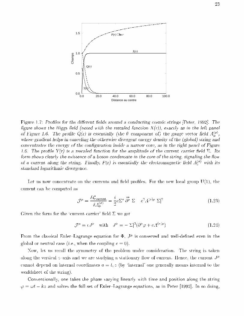
Figure 1.7: Proles for the dierent elds around a conducting cosmic strings [Peter, 1992]. Thegure shows the Higgs eld (noted with the rescaled function X(r)), exactly as in the left panelof Figure 1.6. The prole Q(r) is essentially (the component of) the gauge vector eld A()

,whose gradient helps in canceling the otherwise divergent energy density of the (global) string andconcentrates the energy of the conguration inside a narrow core, as in the right panel of Figure1.6. The prole Y(r) is a rescaled function for the amplitude of the currentcarrier eld . Itsform shows clearly the existence of a boson condensate in the core of the string, signaling the owof a current along the string. Finally, P(r) is essentially the electromagnetic eld A()

z with itsstandard logarithmic divergence.

Let us now concentrate on the currents and eld proles. For the new local group U(1), the

current can be computed as

J =ÆLcurrentÆA()

=i

2e

$

@ e2A()jj2 (1.23)

Given the form for the `current carrier' eld we get

J = eJ with J = jj2(@'+ eA()) (1.24)

From the classical EulerLagrange equation for , J is conserved and well-dened even in the

global or neutral case (i.e., when the coupling e = 0).

Now, let us recall the symmetry of the problem under consideration. The string is taken

along the vertical zaxis and we are studying a stationary ow of current. Hence, the current J

cannot depend on internal coordinates a = t; z (by `internal' one generally means internal to the

worldsheet of the string).

Conventionally, one takes the phase varying linearly with time and position along the string

' = !t kz and solves the full set of EulerLagrange equations, as in Peter [1992]. In so doing,

24

one can write, along the core, Ja = jj2P a and, in turn, Pa(r) = Pa(0)P (r) for each one of

the internal coordinates, this way separating the value at the origin of the conguration from a

common (for both coordinates) rdependent solution P with the condition P (0) = 1. In this

way, one can dene the parameter w (do not confuse with !) such that w = P 2z (0) P 2

t (0) or,

equivalently, P aPa = wP 2. Then the current satises JaJa = jj4wP 2.

The parameter w is important because from its sign one can know in which one of a set of

qualitatively dierent regimes we are working. Actually, w leads to the following classication

[Carter, 1997]

w

8<:> 0 magnetic regime 9 reference frame where Ja is pure spatial

< 0 electric regime 9 reference frame where Ja is mainly charge density

= 0 null

(1.25)

From the solution of the eld equations one gets the standard logarithmic behavior for Pz =

@z'+ eA()z / ln(r) far from the (long) string. This is the expected logarithmic divergence of the

electromagnetic potential around an innite currentcarrier wire with `dc' current I that gives rise

to a magnetic eld B() / 1=r (see Figure 1.7).

1.3.3 Superconducting strings !

One of the most amazing things of the strings we are now treating is the fact that, provided some

general conditions (e.g., the appropriate relation between the free parameters of the model) are

satised, these objects can turn into superconductors. So, under the conditions that the eA term

dominates in the expression for the current J z, we can write

J z = e2jj2Az (1.26)

which is no other than the London equation [London & London, 1935]. From it, recalling the

Faraday's law of the set of Maxwell equations, we can take derivatives on both sides to get

@tJ z = e2jj2Ez: (1.27)

Then, the current grows up linearly in time with an amplitude proportional to the electric eld.

This behavior is exactly the one we would expect for a superconductor [Tinkham, 1995]. In

particular, the equation signals the existence of persistent currents. To see it, just compare with

the corresponding equation for a wire of nite conductivity J z = Ez. One clearly sees in this

equation that when the applied electric eld is turned o, after a certain characteristic time, the

current stops. On the contrary, in Eq. (1.27), when the electric eld vanishes, the current does

not stop but stays constant, i.e., it persists owing along the string.

At suÆciently low temperatures certain materials undergo a phase transition to a new (super-

conducting) phase, characterized notably by the absence of resistance to the passage of currents.

Unlike in these theories, no critical temperature is invoked in here, except for the temperature at

which the condensate forms inside the string, the details of the phase transition being of secondary

25

importance. Moreover, no gap in the excitation spectrum is present, unlike in the solidstate case

where the amount of energy required to excite the system is of the order of that to form a Cooper

pair, and hence the existence of the gap.

The very same considerations of the above paragraphs are valid for fermion (massless) zero

modes along the string [Witten, 1985]. In fact, a generic prediction of these models is the existence

of a maximum current above which the currentcarrying ability of the string saturates. In his

pioneering paper, Witten pointed out that for a fermion of charge q and mass in vacuum m, its

Fermi momentum along the string should be below its mass (in natural units). If this were not

the case, i.e., if the momenta of the fermions exceeded this maximum value, then it would be

energetically favorable for the particle to jump out of the core of the string [Gangui et al., 1999].

This implies that the current saturates and reaches a maximum value

Jmax qmc2

2h(1.28)

If we take electrons as the charge carriers, then one gets currents of size Jmax tens of amperes,

interesting but nothing exceptional (standard superconducting materials at low temperature reach

thousands of amperes and more). On the other hand, if we focus in the early universe and consider

that the current is carried by GUT superheavy fermions, whose normal mass would be around

1016 GeV, then currents more like Jmax 1020A are predicted. Needless to say, these currents are

enormous, even by astrophysical standards!

Und Meissner..? It has long been known that superconductors exclude static magnetic elds

from their interior. This is an eect called the Meissner eect, known since the 1930s and that was

later explained by the BCS (or Bardeen-Cooper-Schrieer) theory in 1957. One can well wonder

what the situation is in our present case, i.e., do currentcarrying cosmic strings show this kind of

behavior?

To answer this question, let us write Ampere's law (in the Coulomb, or radiation, gauge r A =

0)

r2Az = 4J z (1.29)

Also, let us rewrite the London equation

J z = e2jj2Az (1.30)

Putting these two equations together we nd

r2Az = 2Az (1.31)

where we wrote the electromagnetic penetration depth (ej(0)j)1.Roughly, for Cartesian coordinates, if we take x perpendicular to the surface, we have Az /

ex=, which is nothing but the expected exponential decrease of the vector potential inside the

core [Meissner, 1933]. [to be more precise, in the string case we expect r2Pa = e2jj2Pa, withPa = @a'+ eAa].

26

For a lump of standard metal a penetration depth of roughly 105cm is ok. In the string

case, however,

e1j(0)j1 e1v1 (1.32)

which is roughly the Compton wavelength of A. Now, recall that we had v1 > 1, and that

1 was the characteristic (Compton) size of the string core. Hence we nally get that can

be bigger than the size of the string unlike what happens with standard condensedmatter

superconductors, electromagnetic elds can penetrate the string core!

1.3.4 Macroscopic string description

Let us recapitulate brie y the microphysics setting before we see its connection with the macro-

scopic string description we will develop below. We consider a Wittentype bosonic superconduc-

tivity model in which the fundamental Lagrangian is invariant under the action of a U(1)U(1)symmetry group. The rst U(1) is spontaneously broken through the usual Higgs mechanism in

which the Higgs eld acquires a nonvanishing vacuum expectation value. Hence, at an energy

scale ms 1=2 (we will call ms = m hereafter) we are left with a network of ordinary cosmic

strings with tension and energy per unit length T U m2, as dictated by the Kibble mechanism.

The Higgs eld is coupled not only with its associated gauge vector but also with a second

charged scalar boson , the current carrier eld, which in turn obeys a quartic potential. A

second phase transition breaks the second U(1) gauge (or global, in the case of neutral currents)

group and, at an energy scale m, the generation of a currentcarrying condensate in the vortex

makes the tension no longer constant, but dependent on the magnitude of the current, with the

general feature that T m2 U , breaking therefore the degeneracy of the NambuGoto strings

(more below). The fact that jj 6= 0 in the string results in that either electromagnetism (in the

case that the associated gauge vector A() is the electromagnetic potential) or the global U(1) is

spontaneously broken in the core, with the resulting Goldstone bosons carrying charge up and

down the string.

Macroscopic quantities

So, let us dene the relevant macroscopic quantities needed to nd the string equation of state.

For that, we have to rst express the energy momentum tensor as follows

T = 2g ÆL

Æg+ ÆL: (1.33)

One then calculates the macroscopic quantities internal to the string worldsheet (recall `internal'

means coordinates t; z)

T ab = 2ZrdrT ab Ja = 2

ZrdrJa for a; b = t; z (1.34)

The macroscopic charge density/current intensity is dened as

C = 2Zrdr

qjJaJaj = 2

qjwj

Zrdrjj2P (1.35)

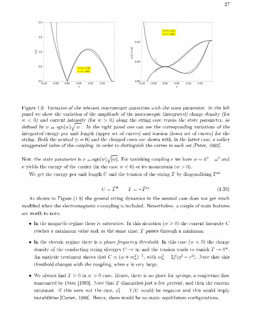
27

−0.10 −0.05 0.00 0.05 0.10 0.15ν

0.0

0.5

1.0

1.5

2.0

C/η

e=0e≠0

−0.10 −0.05 0.00 0.05 0.10 0.15ν

4.90

5.00

5.10

U/η

2 et T

/η2

e=0e≠0

Figure 1.8: Variation of the relevant macroscopic quantities with the state parameter. In the leftpanel we show the variation of the amplitude of the macroscopic (integrated) charge density (forw < 0) and current intensity (for w > 0) along the string core versus the state parameter, as

dened by sgn(w)qjwj. In the right panel one can see the corresponding variations of the

integrated energy per unit length (upper set of curves) and tension (lower set of curves) for thestring. Both the neutral (e = 0) and the charged cases are shown with, in the latter case, a ratherexaggerated value of the coupling, in order to distinguish the curves in each set [Peter, 1992].

Now, the state parameter is sgn(w)qjwj. For vanishing coupling e we have w k2 !2 and

yields the energy of the carrier (in the case w < 0) or its momentum (w > 0).

We get the energy per unit length U and the tension of the string T by diagonalizing T ab

U = T tt T = T zz (1.36)

As shown in Figure (1.8) the general string dynamics in the neutral case does not get much

modied when the electromagnetic e-coupling is included. Nevertheless, a couple of main features

are worth to note:

In the magnetic regime there is saturation. In this situation (w > 0) the current intensity C

reaches a maximum value and, at the same time, T passes through a minimum.

In the electric regime there is a phase frequency threshold. In this case (w < 0) the charge

density of the conducting string diverges C ! 1 and the tension tends to vanish T ! 0+.

An analytic treatment shows that C / (w +m2)

1, with m2 = 2f(2 v2). Note that this

threshold changes with the coupling, when e is very large.

We always nd T > 0 in w > 0 case. Hence, there is no place for springs, a conjecture rst

announced by Peter [1993]. Note that T diminishes just a few percent, and then the current

saturates. If this were not the case, c2T = T=U would be negative and this would imply

instabilities [Carter, 1989]. Hence, there would be no static equilibrium congurations.

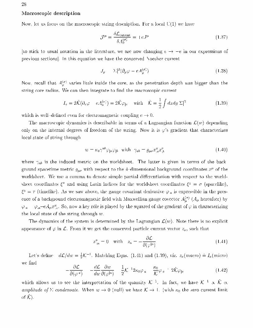
28

Macroscopic description

Now, let us focus on the macroscopic string description. For a local U(1) we have

J =ÆLcurrentÆA

()

= +eJ (1.37)

[to stick to usual notation in the literature, we are now changing e ! e in our expressions of

previous sections]. In this equation we have the conserved Noether current

J = jj2(@' eA() ) (1.38)

Now, recall that A() varies little inside the core, as the penetration depth was bigger than the

string core radius. We can then integrate to nd the macroscopic current

Ia = 2 ~K(@a' eA()a ) = 2 ~K'ja with ~K =

1

2

Zdxdyjj2 (1.39)

which is welldened even for electromagnetic coupling e! 0.

The macroscopic dynamics is describable in terms of a Lagrangian function L(w) dependingonly on the internal degrees of freedom of the string. Now it is ''s gradient that characterizes

local state of string through

w = 0 ab'ja'jb with ab = gx

;ax

;b (1.40)

where ab is the induced metric on the worldsheet. The latter is given in terms of the back-

ground spacetime metric g with respect to the 4dimensional background coordinates x of the

worldsheet. We use a comma to denote simple partial dierentiation with respect to the world-

sheet coordinates a and using Latin indices for the worldsheet coordinates 1 = (spacelike),

0 = (timelike). As we saw above, the gauge covariant derivative 'ja is expressible in the pres-

ence of a background electromagnetic eld with Maxwellian gauge covector A() (A hereafter) by

'ja = ';aeAx;a. So, now a key role is played by the squared of the gradient of ' in characterizing

the local state of the string through w.

The dynamics of the system is determined by the Lagrangian L(w). Note there is no explicit

appearance of ' in L. From it we get the conserved particle current vector za, such that

za;a = 0 with za = @L@('ja)

(1.41)

Let's dene dL=dw = 12K1. Matching Eqns. (1.41) and (1.39), viz. za(macro)

:= Ia(micro)

we nd

@L@('ja)

= dLdw

@w

@('ja)=

1

2K120'ja = 0

K 'ja:= 2 ~K'ja (1.42)

which allows us to see the interpretation of the quantity K1. In fact, we have K1 / ~K /amplitude of -condensate. When w ! 0 (null) we have K ! 1. (with 0 the zero current limit

of ~K).

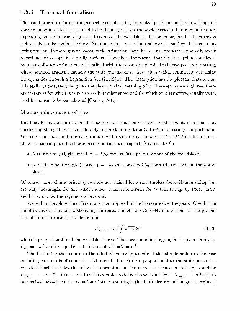
29

1.3.5 The dual formalism

The usual procedure for treating a specic cosmic string dynamical problem consists in writing and

varying an action which is assumed to be the integral over the worldsheet of a Lagrangian function

depending on the internal degrees of freedom of the worldsheet. In particular, for the structureless

string, this is taken to be the GotoNambu action, i.e. the integral over the surface of the constant

string tension. In more general cases, various functions have been suggested that supposedly apply

to various microscopic eld congurations. They share the feature that the description is achieved

by means of a scalar function ', identied with the phase of a physical eld trapped on the string,

whose squared gradient, namely the state parameter w, has values which completely determine

the dynamics through a Lagrangian function L(w). This description has the pleasant feature that

it is easily understandable, given the clear physical meaning of '. However, as we shall see, there

are instances for which it is not so easily implemented and for which an alternative, equally valid,

dual formalism is better adapted [Carter, 1989].

Macroscopic equation of state

But rst, let us concentrate on the macroscopic equation of state. At this point, it is clear that

conducting strings have a considerably richer structure than GotoNambu strings. In particular,

Witten strings have and internal structure with its own equation of state U = U(T ). This, in turn,

allows us to compute the characteristic perturbations speeds [Carter, 1989] :

A transverse (wiggle) speed c2T = T=U for extrinsic perturbations of the worldsheet.

A longitudinal (`woggle') speed c2L = dT=dU for sound-type perturbations within the world-

sheet.

Of course, these characteristic speeds are not dened for a structureless GotoNambu string, but

are fully meaningful for any other model. Numerical results for Witten strings by Peter [1992]

yield cL < cT, i.e. the regime is supersonic.

We will now explore the dierent ansatze proposed in the literature over the years. Clearly, the

simplest case is that one without any currents, namely the GotoNambu action. In the present

formalism it is expressed by the action

SGN = m2Z p d2 (1.43)

which is proportional to string worldsheet area. The corresponding Lagrangian is given simply by

LGN = m2 and its equation of state results U = T = m2.

The rst thing that comes to the mind when trying to extend this simple action to the case

including currents is of course to add a small (linear) term proportional to the state parameter

w, which itself includes the relevant information on the currents. Hence, a rst try would be

Llinear = m2 w2. It turns out that this simple model is also selfdual (with linear = m2

2, to

be precised below) and the equation of state resulting is (for both electric and magnetic regimes)

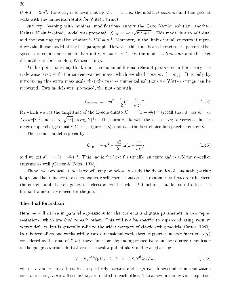
30

U + T = 2m2. However, it follows that cT < cL = 1, i.e., the model is subsonic and this goes at

odds with the numerical results for Witten strings.

2nd try: keeping with minimal modications autour the GotoNambu solution, another,

KaluzaKlein inspired, model was proposed: LKK = mpm2 + w. This model is also selfdual

and the resulting equation of state is UT = m4. Moreover, in the limit of small currents it repro-

duces the linear model of the last paragraph. However, this time both characteristic perturbation

speeds are equal and smaller than unity, cT = cL < 1, i.e. the model is transonic and this fact

disqualies it for modeling Witten strings.

At this point, one may think that there is an additional relevant parameter in the theory, the

scale associated with the currentcarrier mass, which we shall note m (= m). It is only by

introducing this extra mass scale that the precise numerical solutions for Witten strings can be

recovered. Two models were proposed, the rst one with

Lrational = m2 w

2(1 +

w

m2

)1 (1.44)

for which we get the amplitude of the condensate K1 = (1 + wm2

)2 (recall that it was K1 /Rdxdyjj2 and C /

qjwj R dxdyjj2). This ansatz ts well the w ! m2

divergence in the

macroscopic charge density C [see Figure (1.8)] and it is the best choice for spacelike currents.

The second model is given by

Llog = m2 m2

2ln(1 +

w

m2

) (1.45)

and we get K1 = (1 + wm2

)1. This one is the best for timelike currents and is OK for spacelike

currents as well [Carter & Peter, 1995].

These two twoscale models we will employ below to study the dynamics of conducting string

loops and the in uence of electromagnetic selfcorrections on this dynamics at rst order between

the current and the selfgenerated electromagnetic eld. But before that, let us introduce the

formal framework we need for the job.

The dual formalism

Here we will derive in parallel expressions for the currents and state parameters in two repre-

sentations, which are dual to each other. This will not be specic to superconducting vacuum

vortex defects, but is generally valid to the wider category of elastic string models [Carter, 1989].

In this formalism one works with a twodimensional worldsheet supported master function ()

considered as the dual of L(w), these functions depending respectively on the squared magnitude

of the gauge covariant derivative of the scalar potentials and ' as given by

= ~0 ab ja jb ! w =

0 ab'ja'jb ; (1.46)

where 0and ~

0are adjustable, respectively positive and negative, dimensionless normalization

constants that, as we will see below, are related to each other. The arrow in the previous equation

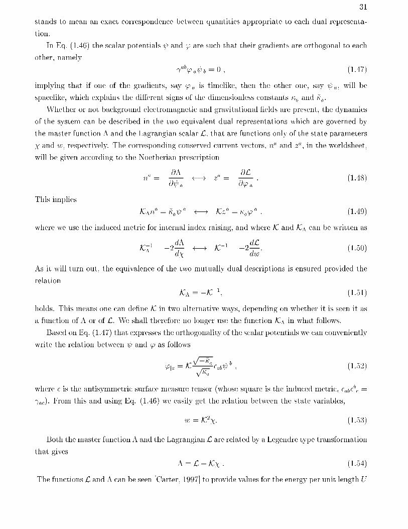
31

stands to mean an exact correspondence between quantities appropriate to each dual representa-

tion.

In Eq. (1.46) the scalar potentials and ' are such that their gradients are orthogonal to each

other, namely

ab'ja jb = 0 ; (1.47)

implying that if one of the gradients, say 'ja is timelike, then the other one, say ja, will be

spacelike, which explains the dierent signs of the dimensionless constants 0and ~

0.

Whether or not background electromagnetic and gravitational elds are present, the dynamics

of the system can be described in the two equivalent dual representations which are governed by

the master function and the Lagrangian scalar L, that are functions only of the state parameters

and w, respectively. The corresponding conserved current vectors, na and za, in the worldsheet,

will be given according to the Noetherian prescription

na = @

@ ja ! za = @L

@'ja: (1.48)

This implies

Kna = ~

0 ja ! Kza =

0'ja ; (1.49)

where we use the induced metric for internal index raising, and where K and K can be written as

K1 = 2dd

! K1 = 2dLdw

: (1.50)

As it will turn out, the equivalence of the two mutually dual descriptions is ensured provided the

relation

K = K1; (1.51)

holds. This means one can dene K in two alternative ways, depending on whether it is seen it as

a function of or of L. We shall therefore no longer use the function K in what follows.

Based on Eq. (1.47) that expresses the orthogonality of the scalar potentials we can conveniently

write the relation between and ' as follows

'ja = Kp~

0p0

ab jb ; (1.52)

where is the antisymmetric surface measure tensor (whose square is the induced metric, abbc =

ac). From this and using Eq. (1.46) we easily get the relation between the state variables,

w = K2: (1.53)

Both the master function and the LagrangianL are related by a Legendre type transformation

that gives

= L+K : (1.54)

The functions L and can be seen [Carter, 1997] to provide values for the energy per unit length U

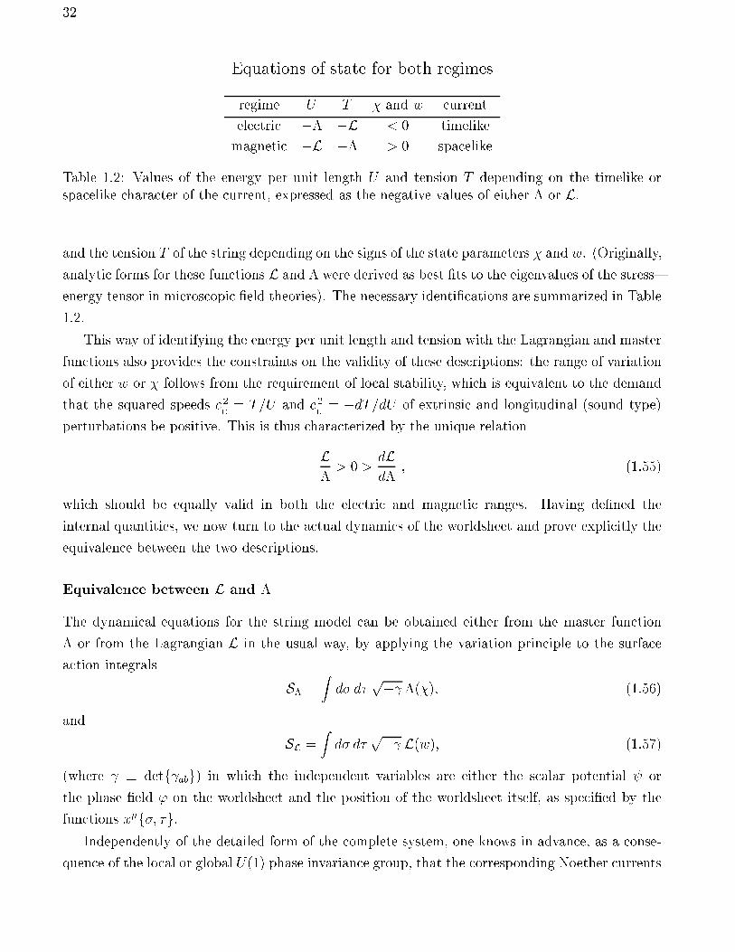
32

Equations of state for both regimes

regime U T and w current

electric L < 0 timelike

magnetic L > 0 spacelike

Table 1.2: Values of the energy per unit length U and tension T depending on the timelike orspacelike character of the current, expressed as the negative values of either or L.

and the tension T of the string depending on the signs of the state parameters and w. (Originally,

analytic forms for these functions L and were derived as best ts to the eigenvalues of the stress

energy tensor in microscopic eld theories). The necessary identications are summarized in Table

1.2.

This way of identifying the energy per unit length and tension with the Lagrangian and master

functions also provides the constraints on the validity of these descriptions: the range of variation

of either w or follows from the requirement of local stability, which is equivalent to the demand

that the squared speeds c 2E= T=U and c 2

L= dT=dU of extrinsic and longitudinal (sound type)

perturbations be positive. This is thus characterized by the unique relation

L> 0 >

dLd

; (1.55)

which should be equally valid in both the electric and magnetic ranges. Having dened the

internal quantities, we now turn to the actual dynamics of the worldsheet and prove explicitly the

equivalence between the two descriptions.

Equivalence between L and

The dynamical equations for the string model can be obtained either from the master function

or from the Lagrangian L in the usual way, by applying the variation principle to the surface

action integrals

S =Zd d

p (); (1.56)

and

SL =Zd d

p L(w); (1.57)

(where detf abg) in which the independent variables are either the scalar potential or

the phase eld ' on the worldsheet and the position of the worldsheet itself, as specied by the

functions xf; g.Independently of the detailed form of the complete system, one knows in advance, as a conse-

quence of the local or global U(1) phase invariance group, that the corresponding Noether currents

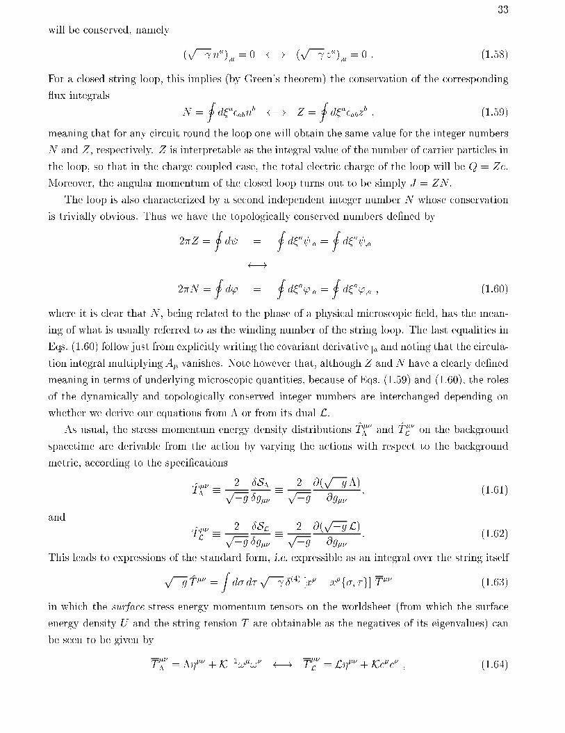
33

will be conserved, namely

(p na);a = 0 ! (

p za);a = 0 : (1.58)

For a closed string loop, this implies (by Green's theorem) the conservation of the corresponding

ux integrals

N =Idaabn

b ! Z =Idaabz

b ; (1.59)

meaning that for any circuit round the loop one will obtain the same value for the integer numbers

N and Z, respectively. Z is interpretable as the integral value of the number of carrier particles in

the loop, so that in the charge coupled case, the total electric charge of the loop will be Q = Ze.

Moreover, the angular momentum of the closed loop turns out to be simply J = ZN .

The loop is also characterized by a second independent integer number N whose conservation

is trivially obvious. Thus we have the topologically conserved numbers dened by

2Z =Id =

Ida ja =

Ida ;a

!

2N =Id' =

Ida'ja =

Ida';a ; (1.60)

where it is clear that N , being related to the phase of a physical microscopic eld, has the mean-

ing of what is usually referred to as the winding number of the string loop. The last equalities in

Eqs. (1.60) follow just from explicitly writing the covariant derivative ja and noting that the circula-

tion integral multiplying A vanishes. Note however that, although Z and N have a clearly dened

meaning in terms of underlying microscopic quantities, because of Eqs. (1.59) and (1.60), the roles

of the dynamically and topologically conserved integer numbers are interchanged depending on

whether we derive our equations from or from its dual L.As usual, the stress momentum energy density distributions T

and T L on the background

spacetime are derivable from the action by varying the actions with respect to the background

metric, according to the specications

T

2pgÆSÆg

2pg@(pg )@g

; (1.61)

and

T L

2pgÆSLÆg

2pg@(pgL)@g

: (1.62)

This leads to expressions of the standard form, i.e. expressible as an integral over the string itself

pg T =Zd d

p Æ(4) [x xf; g] T (1.63)

in which the surface stress energy momentum tensors on the worldsheet (from which the surface

energy density U and the string tension T are obtainable as the negatives of its eigenvalues) can

be seen to be given by

T = +K1!! ! T

L = L + Kcc ; (1.64)

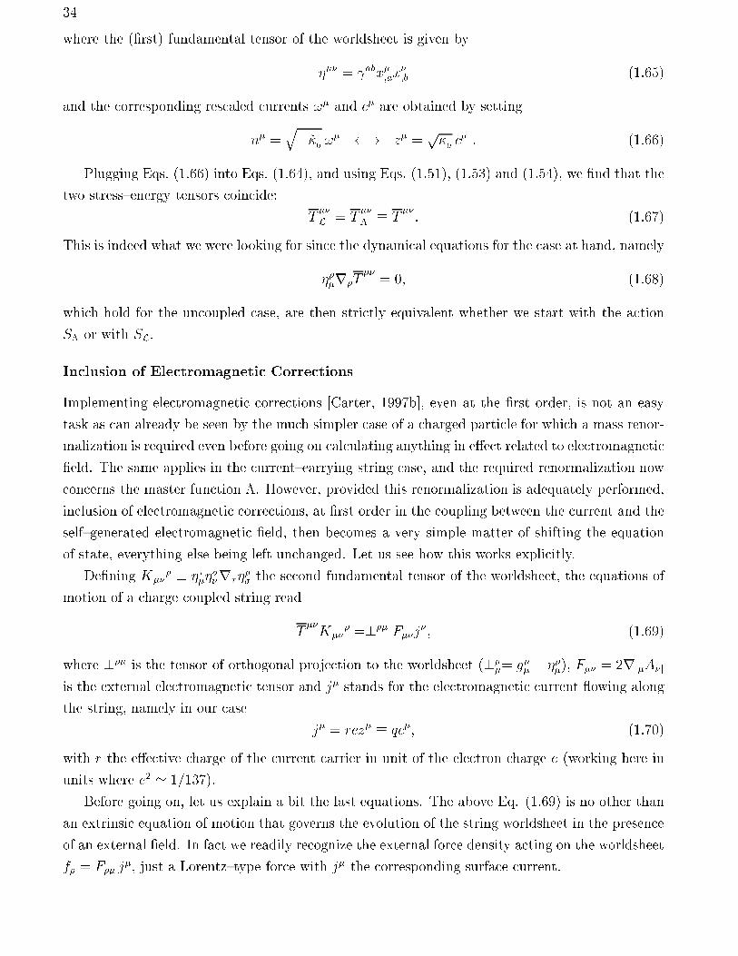
34

where the (rst) fundamental tensor of the worldsheet is given by

= abx;ax;b (1.65)

and the corresponding rescaled currents ! and c are obtained by setting

n =q~

0! ! z =

p0c : (1.66)

Plugging Eqs. (1.66) into Eqs. (1.64), and using Eqs. (1.51), (1.53) and (1.54), we nd that the

two stressenergy tensors coincide:

TL = T

T

: (1.67)

This is indeed what we were looking for since the dynamical equations for the case at hand, namely

rT

= 0; (1.68)

which hold for the uncoupled case, are then strictly equivalent whether we start with the action

S or with SL.

Inclusion of Electromagnetic Corrections

Implementing electromagnetic corrections [Carter, 1997b], even at the rst order, is not an easy

task as can already be seen by the much simpler case of a charged particle for which a mass renor-

malization is required even before going on calculating anything in eect related to electromagnetic

eld. The same applies in the currentcarrying string case, and the required renormalization now

concerns the master function . However, provided this renormalization is adequately performed,

inclusion of electromagnetic corrections, at rst order in the coupling between the current and the

selfgenerated electromagnetic eld, then becomes a very simple matter of shifting the equation

of state, everything else being left unchanged. Let us see how this works explicitly.

Dening K

r

the second fundamental tensor of the worldsheet, the equations of

motion of a charge coupled string read

TK

=? Fj; (1.69)

where ? is the tensor of orthogonal projection to the worldsheet (?= g ), F = 2r[A]

is the external electromagnetic tensor and j stands for the electromagnetic current owing along

the string, namely in our case

j = rez qc; (1.70)

with r the eective charge of the current carrier in unit of the electron charge e (working here in

units where e2 ' 1=137).

Before going on, let us explain a bit the last equations. The above Eq. (1.69) is no other than

an extrinsic equation of motion that governs the evolution of the string worldsheet in the presence

of an external eld. In fact we readily recognize the external force density acting on the worldsheet

f = F j, just a Lorentztype force with j the corresponding surface current.

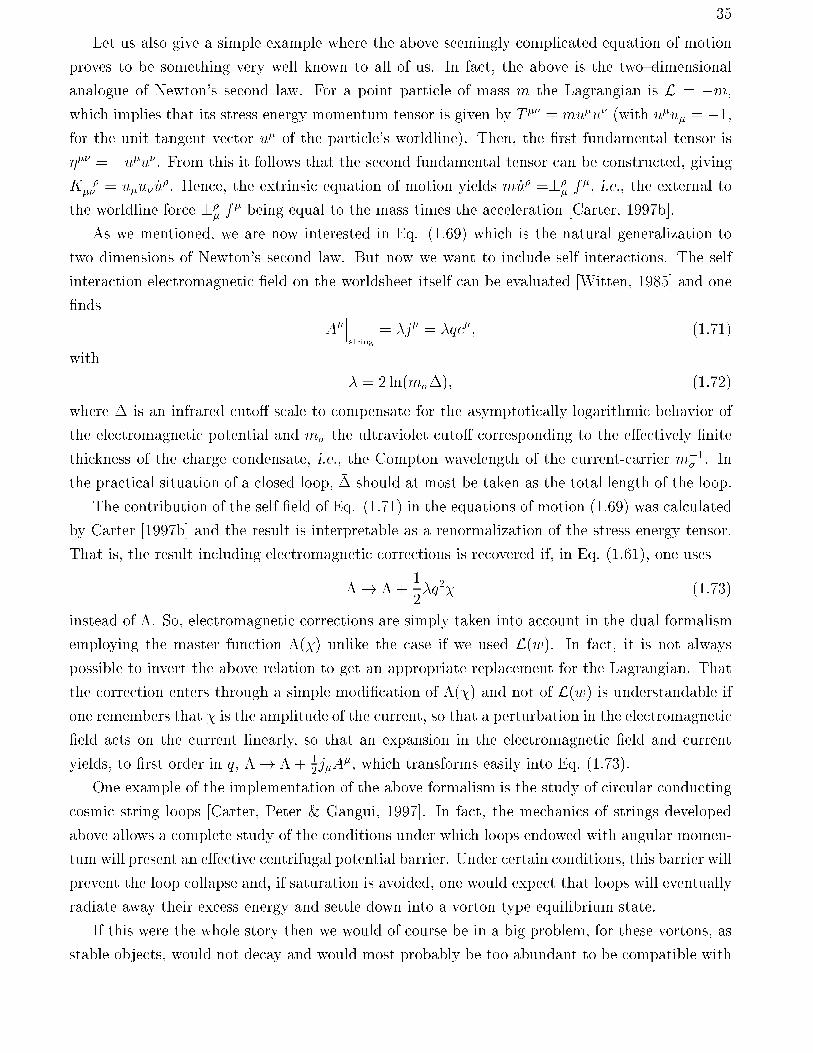
35

Let us also give a simple example where the above seemingly complicated equation of motion

proves to be something very well known to all of us. In fact, the above is the twodimensional

analogue of Newton's second law. For a point particle of mass m the Lagrangian is L = m,

which implies that its stress energy momentum tensor is given by T = muu (with uu = 1,for the unit tangent vector u of the particle's worldline). Then, the rst fundamental tensor is

= uu. From this it follows that the second fundamental tensor can be constructed, giving

K = uu _u

. Hence, the extrinsic equation of motion yields m _u =? f

, i.e., the external to

the worldline force ? f

being equal to the mass times the acceleration [Carter, 1997b].

As we mentioned, we are now interested in Eq. (1.69) which is the natural generalization to

two dimensions of Newton's second law. But now we want to include self interactions. The self

interaction electromagnetic eld on the worldsheet itself can be evaluated [Witten, 1985] and one

nds

Astring

= j = qc; (1.71)

with

= 2 ln(m); (1.72)

where is an infrared cuto scale to compensate for the asymptotically logarithmic behavior of

the electromagnetic potential and m the ultraviolet cuto corresponding to the eectively nite

thickness of the charge condensate, i.e., the Compton wavelength of the current-carrier m1 . In

the practical situation of a closed loop, should at most be taken as the total length of the loop.

The contribution of the self eld of Eq. (1.71) in the equations of motion (1.69) was calculated

by Carter [1997b] and the result is interpretable as a renormalization of the stress energy tensor.

That is, the result including electromagnetic corrections is recovered if, in Eq. (1.61), one uses

! +1

2q2 (1.73)

instead of . So, electromagnetic corrections are simply taken into account in the dual formalism

employing the master function () unlike the case if we used L(w). In fact, it is not always

possible to invert the above relation to get an appropriate replacement for the Lagrangian. That

the correction enters through a simple modication of () and not of L(w) is understandable ifone remembers that is the amplitude of the current, so that a perturbation in the electromagnetic

eld acts on the current linearly, so that an expansion in the electromagnetic eld and current

yields, to rst order in q, ! + 12jA

, which transforms easily into Eq. (1.73).

One example of the implementation of the above formalism is the study of circular conducting

cosmic string loops [Carter, Peter & Gangui, 1997]. In fact, the mechanics of strings developed

above allows a complete study of the conditions under which loops endowed with angular momen-

tum will present an eective centrifugal potential barrier. Under certain conditions, this barrier will

prevent the loop collapse and, if saturation is avoided, one would expect that loops will eventually

radiate away their excess energy and settle down into a vorton type equilibrium state.

If this were the whole story then we would of course be in a big problem, for these vortons, as

stable objects, would not decay and would most probably be too abundant to be compatible with

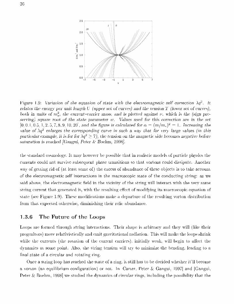
36

−7 −5 −3 −1 1 3 5 7ν

0.0

0.5

1.0

1.5

2.0

2.5

U/m

*2 a

nd T

/m*2

20

01

Figure 1.9: Variation of the equation of state with the electromagnetic selfcorrection q2. Itrelates the energy per unit length U (upper set of curves) and the tension T (lower set of curves),both in units of m2

, the currentcarrier mass, and is plotted against , which is the (sign pre-serving) square root of the state parameter w. Values used for this correction are in the set[0; 0:1; 0:5; 1; 2; 5; 7; 8; 9; 10; 20], and the gure is calculated for = (m=m)

2 = 1. Increasing thevalue of q2 enlarges the corresponding curve in such a way that for very large values (in thisparticular example, it is for for q2 7), the tension on the magnetic side becomes negative beforesaturation is reached [Gangui, Peter & Boehm, 1998].

the standard cosmology. It may however be possible that in realistic models of particle physics the

currents could not survive subsequent phase transitions so that vortons could dissipate. Another

way of getting rid of (at least some of) the excess of abundance of these objects is to take account

of the electromagnetic self interactions in the macroscopic state of the conducting string: as we

said above, the electromagnetic eld in the vicinity of the string will interact with the very same

string current that generated it, with the resulting eect of modifying its macroscopic equation of

state (see Figure 1.9). These modications make a departure of the resulting vorton distribution

from that expected otherwise, diminishing their relic abundance.

1.3.6 The Future of the Loops

Loops are formed through string interactions. Their shape is arbitrary and they will (like their

progenitors) move relativistically and emit gravitational radiation. This will make the loops shrink

while the currents (the rotation of the current carriers), initially weak, will begin to aect the

dynamics at some point. Also, the string tension will try to minimize the bending, leading to a

nal state of a circular and rotating ring.

Once a string loop has reached the state of a ring, it still has to be decided whether it'll become

a vorton (an equilibrium conguration) or not. In [Carter, Peter & Gangui, 1997] and [Gangui,

Peter & Boehm, 1998] we studied the dynamics of circular rings, including the possibility that the

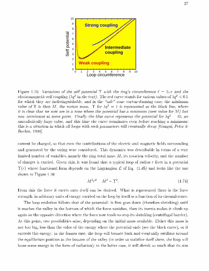
37

0 1 2 3 4 5 6 7 8 9 10Loop circumference

0

1

2

3

4

5

6

7

8

9

10

Sel

f pot

entia

lWeak coupling

Intermediatecoupling

Strong coupling

Figure 1.10: Variations of the self potential with the ring's circumference ` = 2r and theelectromagnetic self coupling (q2 in the text). The red curve stands for various values of q2 < 0:1for which they are indistinguishable, and in the \safe" zone vortonforming case; the minimumvalue of is then M , the vorton mass. for q2 = 1 is represented as the black line, whereit is clear that we now are in a zone where the potential has a minimum (new value for M) butnow terminates at some point. Finally the blue curve represents the potential for q2 = 10, anunrealistically large value, and this time the curve terminates even before reaching a minimum:this is a situation in which all loops with such parameters will eventually decay [Gangui, Peter &Boehm, 1998].

current be charged, so that even the contributions of the electric and magnetic elds surrounding

and generated by the string were considered. This dynamics was describable in terms of a very

limited number of variables, namely the ring total mass M , its rotation velocity, and the number

of charges it carried. Given this, it was found that a typical loop of radius r lives in a potential

(r) whose functional form depends on the Lagrangian L of Eq. (1.45) and looks like the one

shown in Figure 1.10

M2 _r2 =M2 2: (1.74)

From this the force it exerts onto itself can be derived. What is represented there is the force

strength, in arbitrary units of energy, exerted on the loop by itself as a function of its circumference.

The loop evolution follows that of the potential: it rst goes down (therefore shrinking) until

it reaches the valley in the bottom of which the force vanishes, then its inertia makes it climb up

again on the opposite direction where the force now tends to stop its shrinking (centrifugal barrier).

At this point, two possibilities arise, depending on the initial mass available. Either this mass is

not too big, less than the value of the energy where the potential ends (see the black curve), or it

exceeds this energy: in the former case, the loop will bounce back and eventually oscillate around

the equilibrium position at the bottom of the valley (in order to stabilize itself there, the loop will

loose some energy in the form of radiation); in the latter case, it will shrink so much that its size

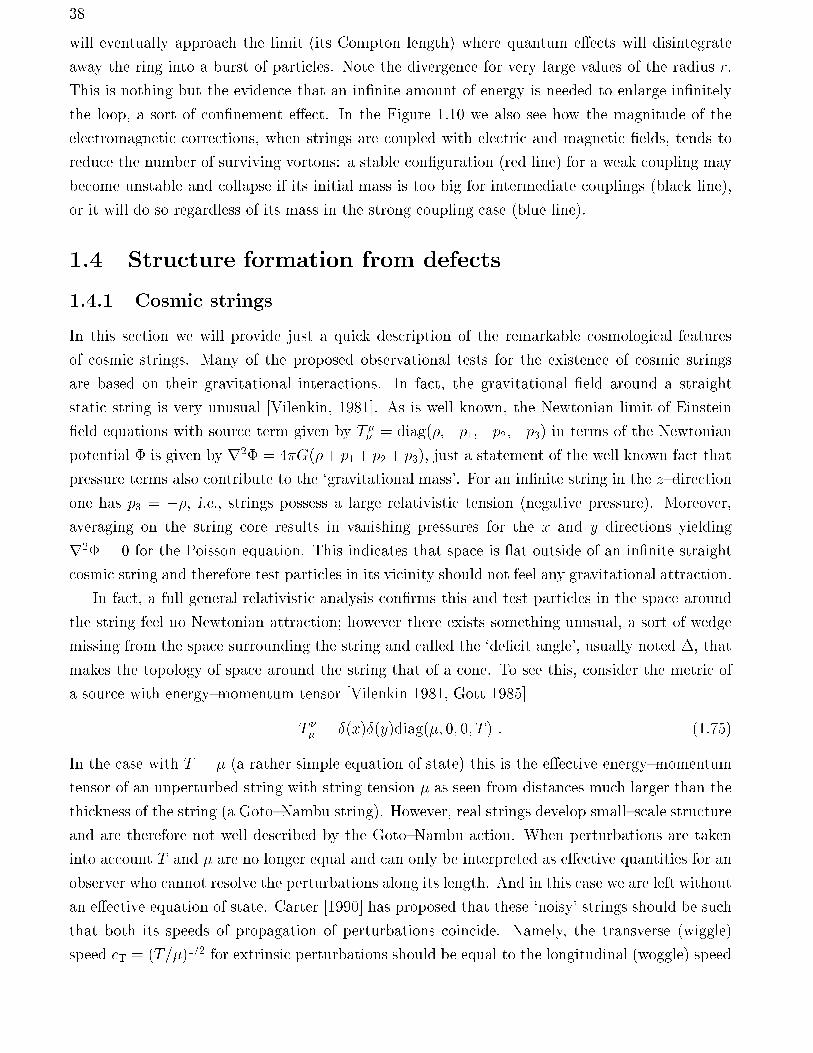
38

will eventually approach the limit (its Compton length) where quantum eects will disintegrate

away the ring into a burst of particles. Note the divergence for very large values of the radius r.

This is nothing but the evidence that an innite amount of energy is needed to enlarge innitely

the loop, a sort of connement eect. In the Figure 1.10 we also see how the magnitude of the

electromagnetic corrections, when strings are coupled with electric and magnetic elds, tends to

reduce the number of surviving vortons: a stable conguration (red line) for a weak coupling may

become unstable and collapse if its initial mass is too big for intermediate couplings (black line),

or it will do so regardless of its mass in the strong coupling case (blue line).

1.4 Structure formation from defects

1.4.1 Cosmic strings

In this section we will provide just a quick description of the remarkable cosmological features

of cosmic strings. Many of the proposed observational tests for the existence of cosmic strings

are based on their gravitational interactions. In fact, the gravitational eld around a straight

static string is very unusual [Vilenkin, 1981]. As is well known, the Newtonian limit of Einstein

eld equations with source term given by T = diag(;p1;p2;p3) in terms of the Newtonian

potential is given by r2 = 4G(+ p1+ p2+ p3), just a statement of the well known fact that

pressure terms also contribute to the `gravitational mass'. For an innite string in the zdirection

one has p3 = , i.e., strings possess a large relativistic tension (negative pressure). Moreover,

averaging on the string core results in vanishing pressures for the x and y directions yielding

r2 = 0 for the Poisson equation. This indicates that space is at outside of an innite straight

cosmic string and therefore test particles in its vicinity should not feel any gravitational attraction.

In fact, a full general relativistic analysis conrms this and test particles in the space around

the string feel no Newtonian attraction; however there exists something unusual, a sort of wedge

missing from the space surrounding the string and called the `decit angle', usually noted , that

makes the topology of space around the string that of a cone. To see this, consider the metric of

a source with energymomentum tensor [Vilenkin 1981, Gott 1985]

T = Æ(x)Æ(y)diag(; 0; 0; T ) : (1.75)

In the case with T = (a rather simple equation of state) this is the eective energymomentum

tensor of an unperturbed string with string tension as seen from distances much larger than the

thickness of the string (a GotoNambu string). However, real strings develop smallscale structure

and are therefore not well described by the GotoNambu action. When perturbations are taken

into account T and are no longer equal and can only be interpreted as eective quantities for an

observer who cannot resolve the perturbations along its length. And in this case we are left without

an eective equation of state. Carter [1990] has proposed that these `noisy' strings should be such

that both its speeds of propagation of perturbations coincide. Namely, the transverse (wiggle)

speed cT = (T=)1=2 for extrinsic perturbations should be equal to the longitudinal (woggle) speed

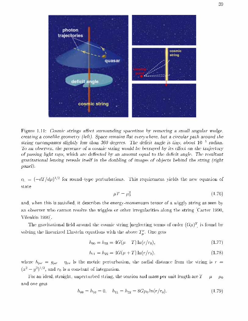
39

Figure 1.11: Cosmic strings aect surrounding spacetime by removing a small angular wedge,creating a conelike geometry (left). Space remains at everywhere, but a circular path around thestring encompasses slightly less than 360 degrees. The decit angle is tiny, about 105 radian.To an observer, the presence of a cosmic string would be betrayed by its eect on the trajectoryof passing light rays, which are de ected by an amount equal to the decit angle. The resultantgravitational lensing reveals itself in the doubling of images of objects behind the string (rightpanel).

cL = (dT=d)1=2 for soundtype perturbations. This requirement yields the new equation of

state

T = 20 (1.76)

and, when this is satised, it describes the energy-momentum tensor of a wiggly string as seen by

an observer who cannot resolve the wiggles or other irregularities along the string [Carter 1990,

Vilenkin 1990].

The gravitational eld around the cosmic string [neglecting terms of order (G)2] is found by

solving the linearized Einstein equations with the above T . One gets

h00 = h33 = 4G( T ) ln(r=r0); (1.77)

h11 = h22 = 4G(+ T ) ln(r=r0); (1.78)

where h = g is the metric perturbation, the radial distance from the string is r =

(x2 + y2)1=2, and r0 is a constant of integration.

For an ideal, straight, unperturbed string, the tension and mass per unit length are T = = 0

and one gets

h00 = h33 = 0; h11 = h22 = 8G0 ln(r=r0): (1.79)

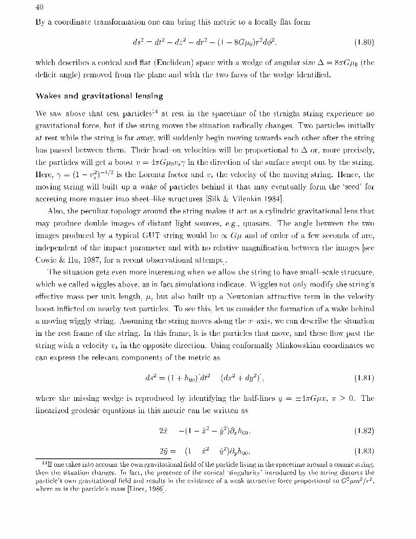
40

By a coordinate transformation one can bring this metric to a locally at form

ds2 = dt2 dz2 dr2 (1 8G0)r2d2; (1.80)

which describes a conical and at (Euclidean) space with a wedge of angular size = 8G0 (the

decit angle) removed from the plane and with the two faces of the wedge identied.

Wakes and gravitational lensing

We saw above that test particles14 at rest in the spacetime of the straight string experience no

gravitational force, but if the string moves the situation radically changes. Two particles initially

at rest while the string is far away, will suddenly begin moving towards each other after the string

has passed between them. Their headon velocities will be proportional to or, more precisely,

the particles will get a boost v = 4G0vs in the direction of the surface swept out by the string.

Here, = (1 v2s)1=2 is the Lorentz factor and vs the velocity of the moving string. Hence, the

moving string will built up a wake of particles behind it that may eventually form the `seed' for

accreting more matter into sheetlike structures [Silk & Vilenkin 1984].

Also, the peculiar topology around the string makes it act as a cylindric gravitational lens that

may produce double images of distant light sources, e.g., quasars. The angle between the two

images produced by a typical GUT string would be / G and of order of a few seconds of arc,

independent of the impact parameter and with no relative magnication between the images [see

Cowie & Hu, 1987, for a recent observational attempt].

The situation gets even more interesting when we allow the string to have smallscale structure,

which we called wiggles above, as in fact simulations indicate. Wiggles not only modify the string's

eective mass per unit length, , but also built up a Newtonian attractive term in the velocity

boost in icted on nearby test particles. To see this, let us consider the formation of a wake behind

a moving wiggly string. Assuming the string moves along the xaxis, we can describe the situation

in the rest frame of the string. In this frame, it is the particles that move, and these ow past the

string with a velocity vs in the opposite direction. Using conformally Minkowskian coordinates we

can express the relevant components of the metric as

ds2 = (1 + h00)[dt2 (dx2 + dy2)]; (1.81)

where the missing wedge is reproduced by identifying the half-lines y = 4Gx, x 0. The

linearized geodesic equations in this metric can be written as

2x = (1 _x2 _y2)@xh00; (1.82)

2y = (1 _x2 _y2)@yh00; (1.83)

14If one takes into account the own gravitational eld of the particle living in the spacetime around a cosmic string,then the situation changes. In fact, the presence of the conical `singularity' introduced by the string distorts theparticle's own gravitational eld and results in the existence of a weak attractive force proportional to G2m2=r2,where m is the particle's mass [Linet, 1986].

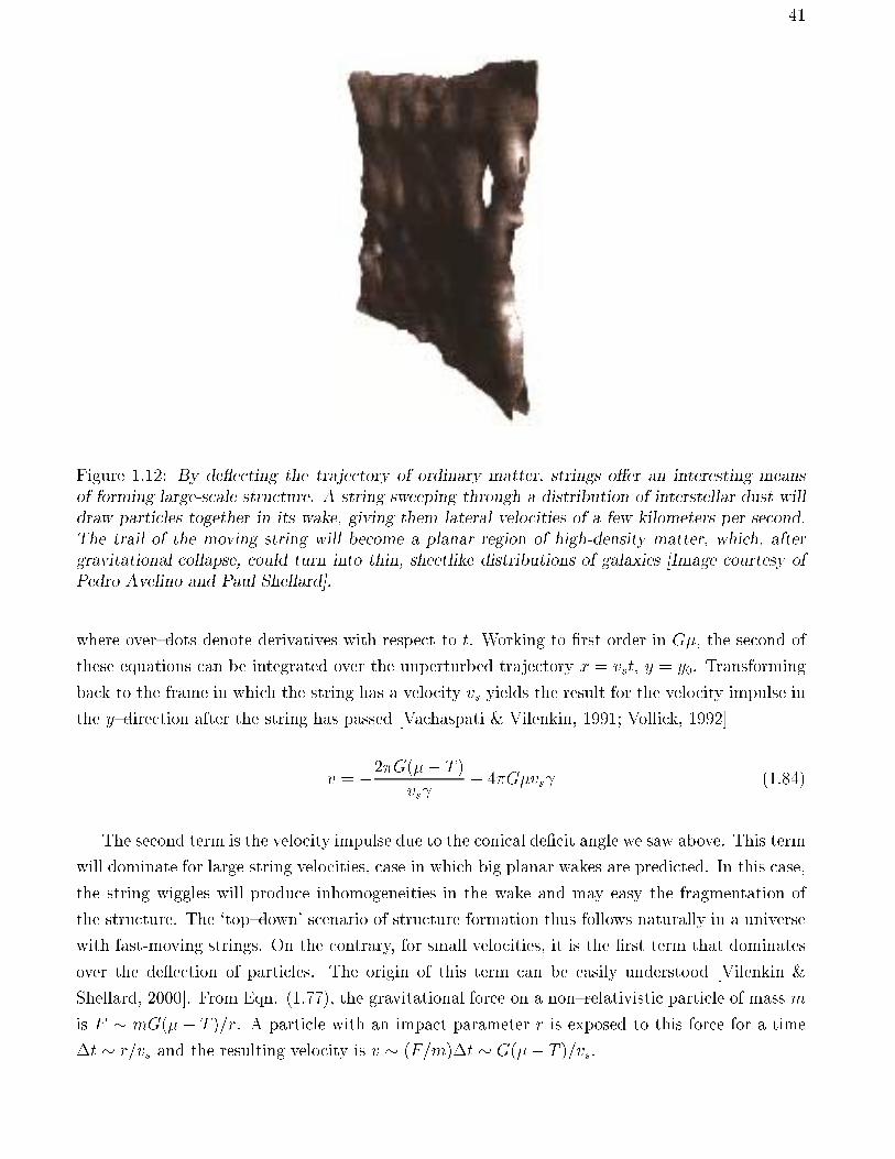
41

Figure 1.12: By de ecting the trajectory of ordinary matter, strings oer an interesting meansof forming large-scale structure. A string sweeping through a distribution of interstellar dust willdraw particles together in its wake, giving them lateral velocities of a few kilometers per second.The trail of the moving string will become a planar region of high-density matter, which, aftergravitational collapse, could turn into thin, sheetlike distributions of galaxies [Image courtesy ofPedro Avelino and Paul Shellard].

where overdots denote derivatives with respect to t. Working to rst order in G, the second of

these equations can be integrated over the unperturbed trajectory x = vst, y = y0. Transforming

back to the frame in which the string has a velocity vs yields the result for the velocity impulse in

the ydirection after the string has passed [Vachaspati & Vilenkin, 1991; Vollick, 1992]

v = 2G( T )vs

4Gvs (1.84)

The second term is the velocity impulse due to the conical decit angle we saw above. This term

will dominate for large string velocities, case in which big planar wakes are predicted. In this case,

the string wiggles will produce inhomogeneities in the wake and may easy the fragmentation of

the structure. The `topdown' scenario of structure formation thus follows naturally in a universe

with fast-moving strings. On the contrary, for small velocities, it is the rst term that dominates

over the de ection of particles. The origin of this term can be easily understood [Vilenkin &

Shellard, 2000]. From Eqn. (1.77), the gravitational force on a nonrelativistic particle of mass m

is F mG( T )=r. A particle with an impact parameter r is exposed to this force for a time

t r=vs and the resulting velocity is v (F=m)t G( T )=vs.

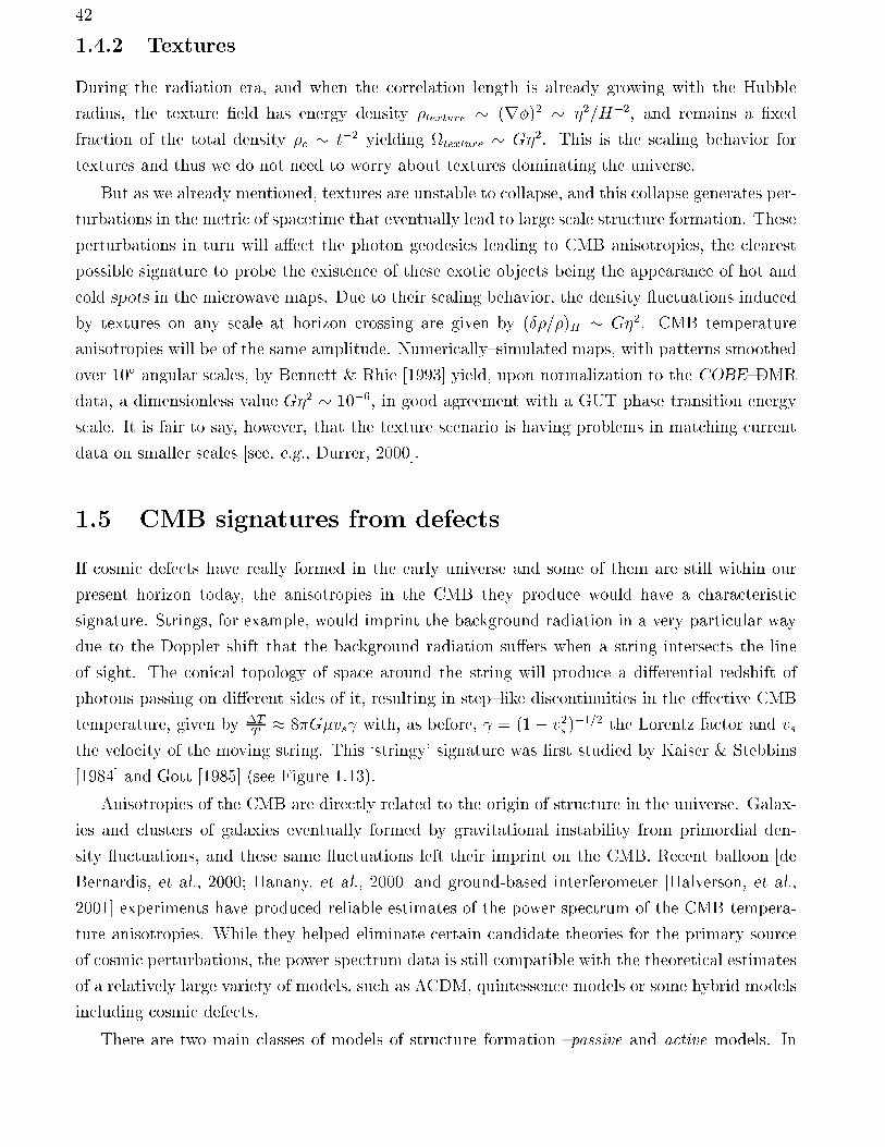
42

1.4.2 Textures

During the radiation era, and when the correlation length is already growing with the Hubble

radius, the texture eld has energy density texture (r)2 2=H2, and remains a xed

fraction of the total density c t2 yielding texture G2. This is the scaling behavior for

textures and thus we do not need to worry about textures dominating the universe.

But as we already mentioned, textures are unstable to collapse, and this collapse generates per-

turbations in the metric of spacetime that eventually lead to large scale structure formation. These

perturbations in turn will aect the photon geodesics leading to CMB anisotropies, the clearest

possible signature to probe the existence of these exotic objects being the appearance of hot and

cold spots in the microwave maps. Due to their scaling behavior, the density uctuations induced

by textures on any scale at horizon crossing are given by (Æ=)H G2. CMB temperature

anisotropies will be of the same amplitude. Numericallysimulated maps, with patterns smoothed

over 10Æ angular scales, by Bennett & Rhie [1993] yield, upon normalization to the COBEDMR

data, a dimensionless value G2 106, in good agreement with a GUT phase transition energy

scale. It is fair to say, however, that the texture scenario is having problems in matching current

data on smaller scales [see, e.g., Durrer, 2000].

1.5 CMB signatures from defects

If cosmic defects have really formed in the early universe and some of them are still within our

present horizon today, the anisotropies in the CMB they produce would have a characteristic

signature. Strings, for example, would imprint the background radiation in a very particular way

due to the Doppler shift that the background radiation suers when a string intersects the line

of sight. The conical topology of space around the string will produce a dierential redshift of

photons passing on dierent sides of it, resulting in steplike discontinuities in the eective CMB

temperature, given by TT 8Gvs with, as before, = (1 v2s)1=2 the Lorentz factor and vs

the velocity of the moving string. This `stringy' signature was rst studied by Kaiser & Stebbins

[1984] and Gott [1985] (see Figure 1.13).

Anisotropies of the CMB are directly related to the origin of structure in the universe. Galax-

ies and clusters of galaxies eventually formed by gravitational instability from primordial den-

sity uctuations, and these same uctuations left their imprint on the CMB. Recent balloon [de

Bernardis, et al., 2000; Hanany, et al., 2000] and ground-based interferometer [Halverson, et al.,

2001] experiments have produced reliable estimates of the power spectrum of the CMB tempera-

ture anisotropies. While they helped eliminate certain candidate theories for the primary source

of cosmic perturbations, the power spectrum data is still compatible with the theoretical estimates

of a relatively large variety of models, such as CDM, quintessence models or some hybrid models

including cosmic defects.

There are two main classes of models of structure formation passive and active models. In

43

Figure 1.13: The Kaiser-Stebbins eect for cosmic strings. A string network evolves into a self-similar scaling regime, perturbing matter and radiation during its evolution. The eect on theCMB after recombination leads to distinct steplike discontinuities on small angular scales thatwere rst studied by Kaiser & Stebbins [1984]. The left panel shows a simulated patch of the skythat ts in one of the pixels of the COBE experiment. Hence, higher resolution observatories areneeded in order to detect strings. The right panel shows a patch on the CMB sky of order 20'across. However, recent studies indicate that this clean tell-tale signal gets obscured at subdegreeangular scales due to the temperature uctuations generated before recombination. [Magueijo &Ferreira 1997].

passive models, density inhomogeneities are set as initial conditions at some early time, and while

they subsequently evolve as described by EinsteinBoltzmann equations, no additional perturba-

tions are seeded. On the other hand, in active models the sources of density perturbations are

timedependent.

All specic realizations of passive models are based on the idea of in ation. In simplest in a-

tionary models it is assumed that there exists a weakly coupled scalar eld , called the in aton,

which \drives" the (quasi) exponential expansion of the universe. The quantum uctuations of

are stretched by the expansion to scales beyond the horizon, thus \freezing" their amplitude.

In ation is followed by a period of thermalization, during which standard forms of matter and

energy are formed. Because of the spatial variations of introduced by quantum uctuations,

thermalization occurs at slightly dierent times in dierent parts of the universe. Such uctua-

tions in the thermalization time give rise to density uctuations. Because of their quantum nature

and because of the fact that initial perturbations are assumed to be in the vacuum state and hence

well described by a Gaussian distribution, perturbations produced during in ation are expected

to follow Gaussian statistics to a high degree [Gangui, Lucchin, Matarrese & Mollerach, 1994], or

either be products of Gaussian random variables. This is a fairly general prediction that will be

44

tested shortly with MAP and more thoroughly in the future with Planck.15

Active models of structure formation are motivated by cosmic topological defects with the most

promising candidates being cosmic strings. As we saw in previous sections, it is widely believed

that the universe underwent a series of phase transitions as it cooled down due to the expansion.

If our ideas about grand unication are correct, then some cosmic defects should have formed

during phase transitions in the early universe. Once formed, cosmic strings could survive long

enough to seed density perturbations. Defect models possess the attractive feature that they have

no parameter freedom, as all the necessary information is in principle contained in the underlying

particle physics model. Generically, perturbations produced by active models are not expected to

be Gaussian distributed [Gangui, Pogosian & Winitzki, 2001a].

1.5.1 CMB power spectrum from strings

The narrow main peak and the presence of the second and the third peaks in the CMB angular

power spectrum, as measured by BOOMERANG, MAXIMA and DASI [de Bernardis, et al.,

2000; Hanany, et al., 2000; Halverson, et al., 2001], is an evidence for coherent oscillations of the

photonbaryon uid at the beginning of the decoupling epoch [see, e.g., Gangui, 2001]. While

such coherence is a property of all passive model, realistic cosmic string models produce highly

incoherent perturbations that result in a much broader main peak. This excludes cosmic strings

as the primary source of density uctuations unless new physics is postulated, e.g. models with a

varying speed of light [Avelino & Martins, 2000]. In addition to purely active or passive models,

it has been recently suggested that perturbations could be seeded by some combination of the two

mechanisms. For example, cosmic strings could have formed just before the end of in ation and

partially contributed to seeding density uctuations. It has been shown [Contaldi, et al., 1999;

Battye & Weller, 2000; Bouchet, et al., 2001] that such hybrid models can be rather successful in

tting the CMB power spectrum data.

Calculating CMB anisotropies sourced by topological defects is a rather diÆcult task. In

in ationary scenario the entire information about the seeds is contained in the initial conditions

for the perturbations in the metric. In the case of cosmic defects, perturbations are continuously

seeded over the period of time from the phase transition that had produced them until today.

The exact determination of the resulting anisotropy requires, in principle, the knowledge of the

energymomentum tensor [or, if only two point functions are being calculated, the unequal time

correlators, Pen, Seljak, & Turok, 1997] of the defect network and the products of its decay at

all times. This information is simply not available! Instead, a number of clever simplications,

based on the expected properties of the defect networks (e.g. scaling), are used to calculate the

source. The latest data from BOOMERANG and MAXIMA experiments clearly disagree with the

predictions of these simple models of defects [Durrer, Gangui & Sakellariadou, 1996].

The shape of the CMB angular power spectrum is determined by three main factors: the

15Useful CMB resources can be found at http://www.mpa-garching.mpg.de/~banday/CMB.html

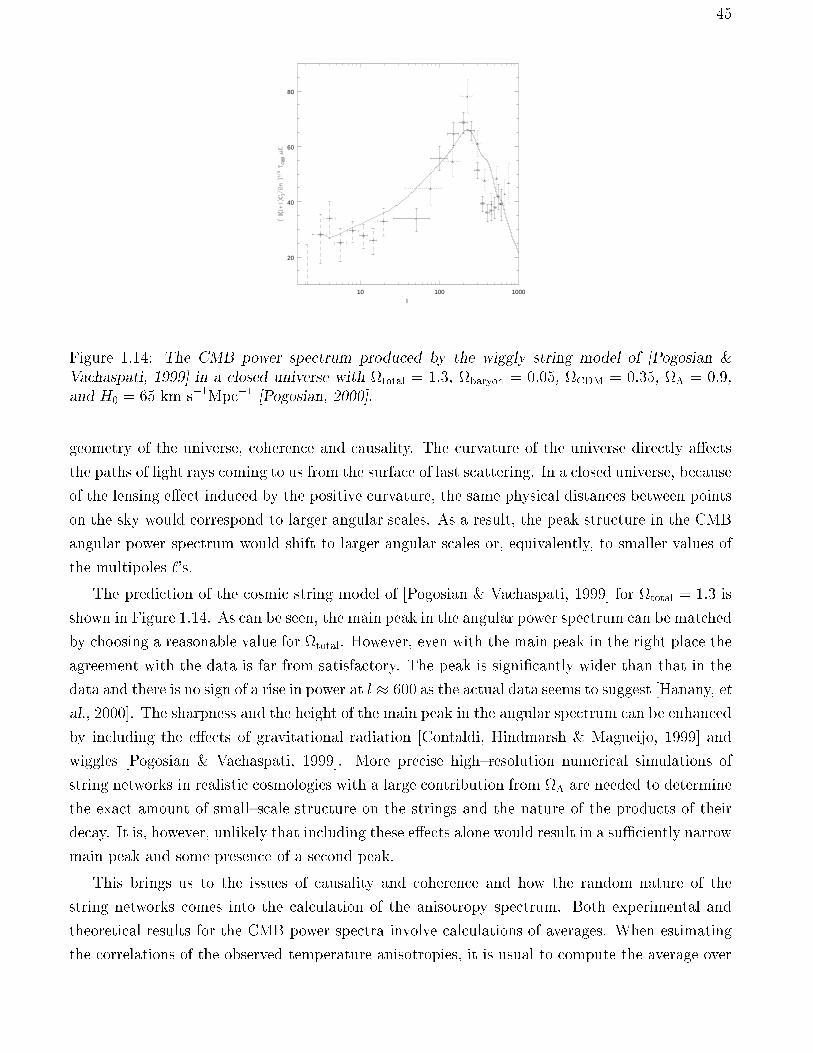
45

10 100 1000

20

40

60

80

l

Figure 1.14: The CMB power spectrum produced by the wiggly string model of [Pogosian &Vachaspati, 1999] in a closed universe with total = 1:3, baryon = 0:05, CDM = 0:35, = 0:9,and H0 = 65 km s1Mpc1 [Pogosian, 2000].

geometry of the universe, coherence and causality. The curvature of the universe directly aects

the paths of light rays coming to us from the surface of last scattering. In a closed universe, because

of the lensing eect induced by the positive curvature, the same physical distances between points

on the sky would correspond to larger angular scales. As a result, the peak structure in the CMB

angular power spectrum would shift to larger angular scales or, equivalently, to smaller values of

the multipoles `'s.

The prediction of the cosmic string model of [Pogosian & Vachaspati, 1999] for total = 1:3 is

shown in Figure 1.14. As can be seen, the main peak in the angular power spectrum can be matched

by choosing a reasonable value for total. However, even with the main peak in the right place the

agreement with the data is far from satisfactory. The peak is signicantly wider than that in the

data and there is no sign of a rise in power at l 600 as the actual data seems to suggest [Hanany, et

al., 2000]. The sharpness and the height of the main peak in the angular spectrum can be enhanced

by including the eects of gravitational radiation [Contaldi, Hindmarsh & Magueijo, 1999] and

wiggles [Pogosian & Vachaspati, 1999]. More precise highresolution numerical simulations of

string networks in realistic cosmologies with a large contribution from are needed to determine

the exact amount of smallscale structure on the strings and the nature of the products of their

decay. It is, however, unlikely that including these eects alone would result in a suÆciently narrow

main peak and some presence of a second peak.

This brings us to the issues of causality and coherence and how the random nature of the

string networks comes into the calculation of the anisotropy spectrum. Both experimental and

theoretical results for the CMB power spectra involve calculations of averages. When estimating

the correlations of the observed temperature anisotropies, it is usual to compute the average over

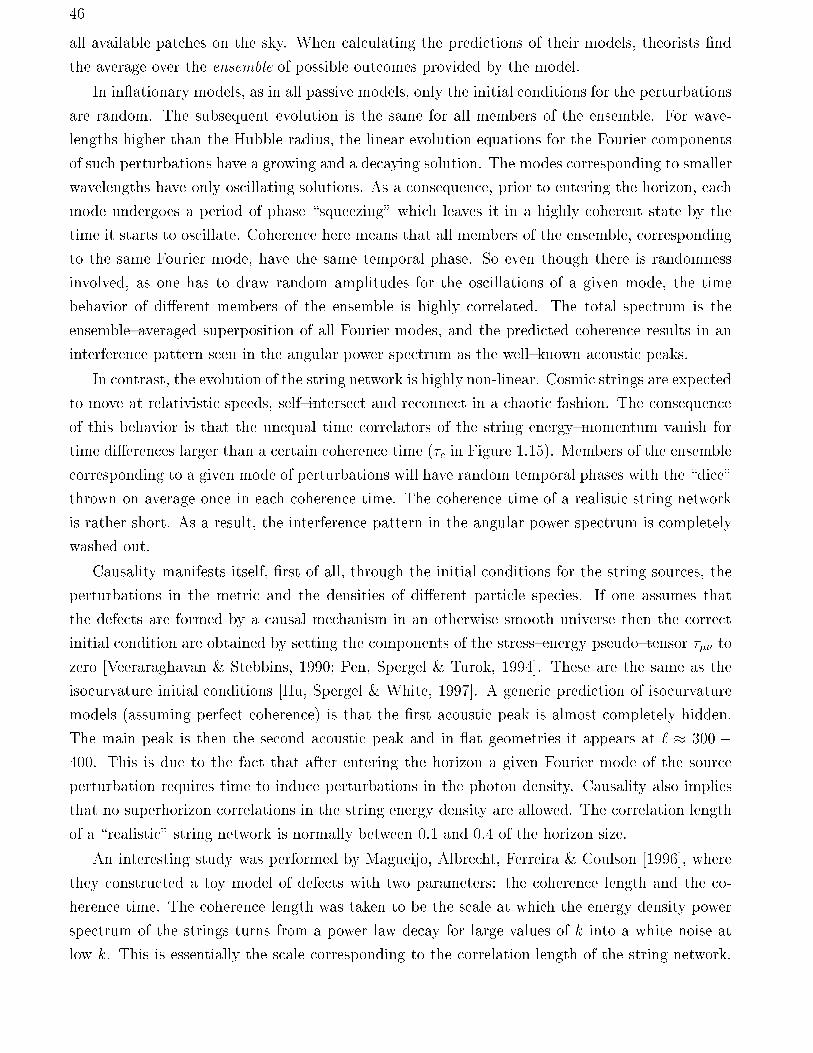
46

all available patches on the sky. When calculating the predictions of their models, theorists nd

the average over the ensemble of possible outcomes provided by the model.

In in ationary models, as in all passive models, only the initial conditions for the perturbations

are random. The subsequent evolution is the same for all members of the ensemble. For wave-

lengths higher than the Hubble radius, the linear evolution equations for the Fourier components

of such perturbations have a growing and a decaying solution. The modes corresponding to smaller

wavelengths have only oscillating solutions. As a consequence, prior to entering the horizon, each

mode undergoes a period of phase \squeezing" which leaves it in a highly coherent state by the

time it starts to oscillate. Coherence here means that all members of the ensemble, corresponding

to the same Fourier mode, have the same temporal phase. So even though there is randomness

involved, as one has to draw random amplitudes for the oscillations of a given mode, the time

behavior of dierent members of the ensemble is highly correlated. The total spectrum is the

ensembleaveraged superposition of all Fourier modes, and the predicted coherence results in an

interference pattern seen in the angular power spectrum as the wellknown acoustic peaks.

In contrast, the evolution of the string network is highly non-linear. Cosmic strings are expected

to move at relativistic speeds, selfintersect and reconnect in a chaotic fashion. The consequence

of this behavior is that the unequal time correlators of the string energymomentum vanish for

time dierences larger than a certain coherence time (c in Figure 1.15). Members of the ensemble

corresponding to a given mode of perturbations will have random temporal phases with the \dice"

thrown on average once in each coherence time. The coherence time of a realistic string network

is rather short. As a result, the interference pattern in the angular power spectrum is completely

washed out.

Causality manifests itself, rst of all, through the initial conditions for the string sources, the

perturbations in the metric and the densities of dierent particle species. If one assumes that

the defects are formed by a causal mechanism in an otherwise smooth universe then the correct

initial condition are obtained by setting the components of the stressenergy pseudotensor to

zero [Veeraraghavan & Stebbins, 1990; Pen, Spergel & Turok, 1994]. These are the same as the

isocurvature initial conditions [Hu, Spergel & White, 1997]. A generic prediction of isocurvature

models (assuming perfect coherence) is that the rst acoustic peak is almost completely hidden.

The main peak is then the second acoustic peak and in at geometries it appears at ` 300 400. This is due to the fact that after entering the horizon a given Fourier mode of the source

perturbation requires time to induce perturbations in the photon density. Causality also implies

that no superhorizon correlations in the string energy density are allowed. The correlation length

of a \realistic" string network is normally between 0.1 and 0.4 of the horizon size.

An interesting study was performed by Magueijo, Albrecht, Ferreira & Coulson [1996], where

they constructed a toy model of defects with two parameters: the coherence length and the co-

herence time. The coherence length was taken to be the scale at which the energy density power

spectrum of the strings turns from a power law decay for large values of k into a white noise at

low k. This is essentially the scale corresponding to the correlation length of the string network.

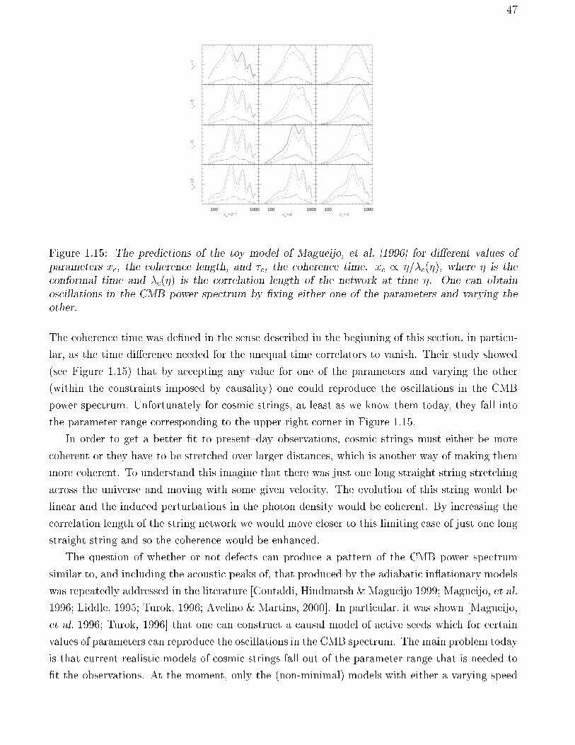
47

100 1000 100 1000 100 1000

Figure 1.15: The predictions of the toy model of Magueijo, et al. [1996] for dierent values ofparameters xc, the coherence length, and c, the coherence time. xc / =c(), where is theconformal time and c() is the correlation length of the network at time . One can obtainoscillations in the CMB power spectrum by xing either one of the parameters and varying theother.

The coherence time was dened in the sense described in the beginning of this section, in particu-

lar, as the time dierence needed for the unequal time correlators to vanish. Their study showed

(see Figure 1.15) that by accepting any value for one of the parameters and varying the other

(within the constraints imposed by causality) one could reproduce the oscillations in the CMB

power spectrum. Unfortunately for cosmic strings, at least as we know them today, they fall into

the parameter range corresponding to the upper right corner in Figure 1.15.

In order to get a better t to presentday observations, cosmic strings must either be more

coherent or they have to be stretched over larger distances, which is another way of making them

more coherent. To understand this imagine that there was just one long straight string stretching

across the universe and moving with some given velocity. The evolution of this string would be

linear and the induced perturbations in the photon density would be coherent. By increasing the

correlation length of the string network we would move closer to this limiting case of just one long

straight string and so the coherence would be enhanced.

The question of whether or not defects can produce a pattern of the CMB power spectrum

similar to, and including the acoustic peaks of, that produced by the adiabatic in ationary models

was repeatedly addressed in the literature [Contaldi, Hindmarsh & Magueijo 1999; Magueijo, et al.

1996; Liddle, 1995; Turok, 1996; Avelino & Martins, 2000]. In particular, it was shown [Magueijo,

et al. 1996; Turok, 1996] that one can construct a causal model of active seeds which for certain

values of parameters can reproduce the oscillations in the CMB spectrum. The main problem today

is that current realistic models of cosmic strings fall out of the parameter range that is needed to

t the observations. At the moment, only the (non-minimal) models with either a varying speed

48

of light or hybrid contribution of strings+in ation are the only ones involving topological defects

that to some extent can match the observations. One possible way to distinguish their predictions

from those of in ationary models would be by computing key nonGaussian statistical quantities,

such as the CMB bispectrum.

1.5.2 CMB bispectrum from active models

Dierent cosmological models dier in their predictions for the statistical distribution of the

anisotropies beyond the power spectrum. Future MAP and Planck satellite missions will pro-

vide high-precision data allowing denite estimates of non-Gaussian signals in the CMB. It is

therefore important to know precisely which are the predictions of all candidate models for the

statistical quantities that will be extracted from the new data and identify their specic signatures.

Of the available non-Gaussian statistics, the CMB bispectrum, or the three-point function of

Fourier components of the temperature anisotropy, has been perhaps the one best studied in the

literature [Gangui & Martin, 2000a]. There are a few cases where the bispectrum may be deduced

analytically from the underlying model. The bispectrum can be estimated from simulated CMB

sky maps; however, computing a large number of full-sky maps resulting from defects is a much

more demanding task. Recently, a precise numerical code to compute it, not using CMB maps and

similar to the CMBFAST code16 for the power spectrum, was developed in [Gangui, Pogosian &

Winitzki 2001b]. What follows below is an account of this work.

In a few words, given a suitable model, one can generate a statistical ensemble of realizations

of defect matter perturbations. We used a modied Boltzmann code based on CMBFAST to

compute the eect of these perturbations on the CMB and found the bispectrum estimator for

a given realization of sources. We then performed statistical averaging over the ensemble of

realizations to compute the expected CMB bispectrum. (The CMB power spectrum was also

obtained as a byproduct.) As a rst application, we then computed the expected CMB bispectrum

from a model of simulated string networks rst introduced by Albrecht et al. [1997] and further

developed in [Pogosian & Vachaspati, 1999] and in [Gangui, Pogosian & Winitzki 2001].

We assume that, given a model of active perturbations, such as a string simulation, we can

calculate the energy-momentum tensor T(x; ) for a particular realization of the sources in a

nite spatial volume V0. Here, x is a 3-dimensional coordinate and is the cosmic time. Many

simulations are run to obtain an ensemble of random realizations of sources with statistical prop-

erties appropriate for the given model. The spatial Fourier decomposition of T can be written

as

T(x; ) =Xk

(k; )eikx ; (1.85)

where k are discrete. If V0 is suÆciently large we can approximate the summation by the integral

Xk

(k; )eikx V0

(2)3

Zd3k(k; )e

ikx ; (1.86)

16http://physics.nyu.edu/matiasz/CMBFAST/cmbfast.html

49

and the corresponding inverse Fourier transform will be

(k; ) =1V0

ZV0d3xT(x; )e

ikx : (1.87)

Of course, the nal results, such as the CMB power spectrum or bispectrum, do not depend on

the choice of V0. To ensure this independence, we shall keep V0 in all expressions where it appears

below.

It is conventional to expand the temperature uctuations over the basis of spherical harmonics,

T=T (n) =Xlm

almYlm(n); (1.88)

where n is a unit vector. The coeÆcients alm can be decomposed into Fourier modes,

alm = V0(2)3

(i)l 4Zd3kl (k)Y

lm(k): (1.89)

Given the sources (k; ), the quantities l(k) are found by solving linearized Einstein-

Boltzmann equations and integrating along the line of sight, using a code similar to CMBFAST

[Seljak & Zaldarriaga, 1996]. This standard procedure can be written symbolically as the action

of a linear operator Bl (k) on the source energy-momentum tensor, l(k) = B

l (k)(k; ), so

the third moment of l(k) is linearly related to the three-point correlator of (k; ). Below we

consider the quantities l(k), corresponding to a set of realizations of active sources, as given. The

numerical procedure for computing l(k) was developed in [Albrecht et al. 1997] and in [Pogosian

& Vachaspati, 1999].

The third moment of alm, namely hal1m1al2m2

al3m3i, can be expressed as

(i)l1+l2+l3 (4)3 V 30

(2)9

Zd3k1d

3k2d3k3Y

l1m1

(k1)Yl2m2

(k2)Yl3m3

(k3) hl1(k1)l2(k2)l3(k3)i : (1.90)

A straightforward numerical evaluation of Eq. (1.90) from given sources l (k) is prohibitively

diÆcult, because it involves too many integrations of oscillating functions. However, we shall be

able to reduce the computation to integrations over scalars [a similar method was employed in

Komatsu & Spergel, 2001 and in Wang & Kamionkowski, 2000]. Due to homogeneity, the 3-point

function vanishes unless the triangle constraint is satised,

k1 + k2 + k3 = 0: (1.91)

We may write

hl1 (k1)l2 (k2)l3 (k3)i = Æ(3) (k1 + k2 + k3)Pl1l2l3 (k1;k2;k3) ; (1.92)

where the three-point function Pl1l2l3 (k1;k2;k3) is dened only for values of ki that satisfy

Eq. (1.91). Given the scalar values k1, k2, k3, there is a unique (up to an overall rotation) triplet

of directions ki for which the RHS of Eq. (1.92) does not vanish. The quantity Pl1l2l3 (k1;k2;k3)

is invariant under an overall rotation of all three vectors ki and therefore may be equivalently

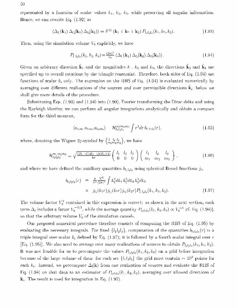
50

represented by a function of scalar values k1, k2, k3, while preserving all angular information.

Hence, we can rewrite Eq. (1.92) as

hl1(k1)l2(k2)l3(k3)i = Æ(3) (k1 + k2 + k3)Pl1l2l3(k1; k2; k3): (1.93)

Then, using the simulation volume V0 explicitly, we have

Pl1l2l3(k1; k2; k3)=(2)3

V0hl1(k1)l2(k2)l3(k3)i : (1.94)

Given an arbitrary direction k1 and the magnitudes k1, k2 and k3, the directions k2 and k3 are

specied up to overall rotations by the triangle constraint. Therefore, both sides of Eq. (1.94) are

functions of scalar ki only. The expression on the RHS of Eq. (1.94) is evaluated numerically by

averaging over dierent realizations of the sources and over permissible directions ki; below we

shall give more details of the procedure.

Substituting Eqs. (1.93) and (1.94) into (1.90), Fourier transforming the Dirac delta and using

the Rayleigh identity, we can perform all angular integrations analytically and obtain a compact

form for the third moment,

hal1m1al2m2

al3m3i = Hm1m2m3

l1l2l3

Zr2dr bl1l2l3(r); (1.95)

where, denoting the Wigner 3j-symbol byl1 l2 l3m1m2m3

, we have

Hm1m2m3

l1l2l3q

(2l1+1)(2l2+1)(2l3+1)4

l1 l2 l30 0 0

! l1 l2 l3m1 m2 m3

!; (1.96)

and where we have dened the auxiliary quantities bl1l2l3 using spherical Bessel functions jl,

bl1l2l3(r) 83

V 30

(2)3

Zk21dk1 k

22dk2 k

23dk3

jl1(k1r)jl2(k2r)jl3(k3r)Pl1l2l3(k1; k2; k3): (1.97)

The volume factor V 30 contained in this expression is correct: as shown in the next section, each

term l includes a factor V2=30 , while the average quantity Pl1l2l3(k1; k2; k3) / V 3

0 [cf. Eq. (1.94)],

so that the arbitrary volume V0 of the simulation cancels.

Our proposed numerical procedure therefore consists of computing the RHS of Eq. (1.95) by

evaluating the necessary integrals. For xed fl1l2l3g, computation of the quantities bl1l2l3(r) is a

triple integral over scalar ki dened by Eq. (1.97); it is followed by a fourth scalar integral over r

[Eq. (1.95)]. We also need to average over many realizations of sources to obtain Pl1l2l3(k1; k2; k3).

It was not feasible for us to precompute the values Pl1l2l3(k1; k2; k3) on a grid before integration

because of the large volume of data: for each set fl1l2l3g the grid must contain 103 points for

each ki. Instead, we precompute l(k) from one realization of sources and evaluate the RHS of

Eq. (1.94) on that data as an estimator of Pl1l2l3(k1; k2; k3), averaging over allowed directions of

ki. The result is used for integration in Eq. (1.97).

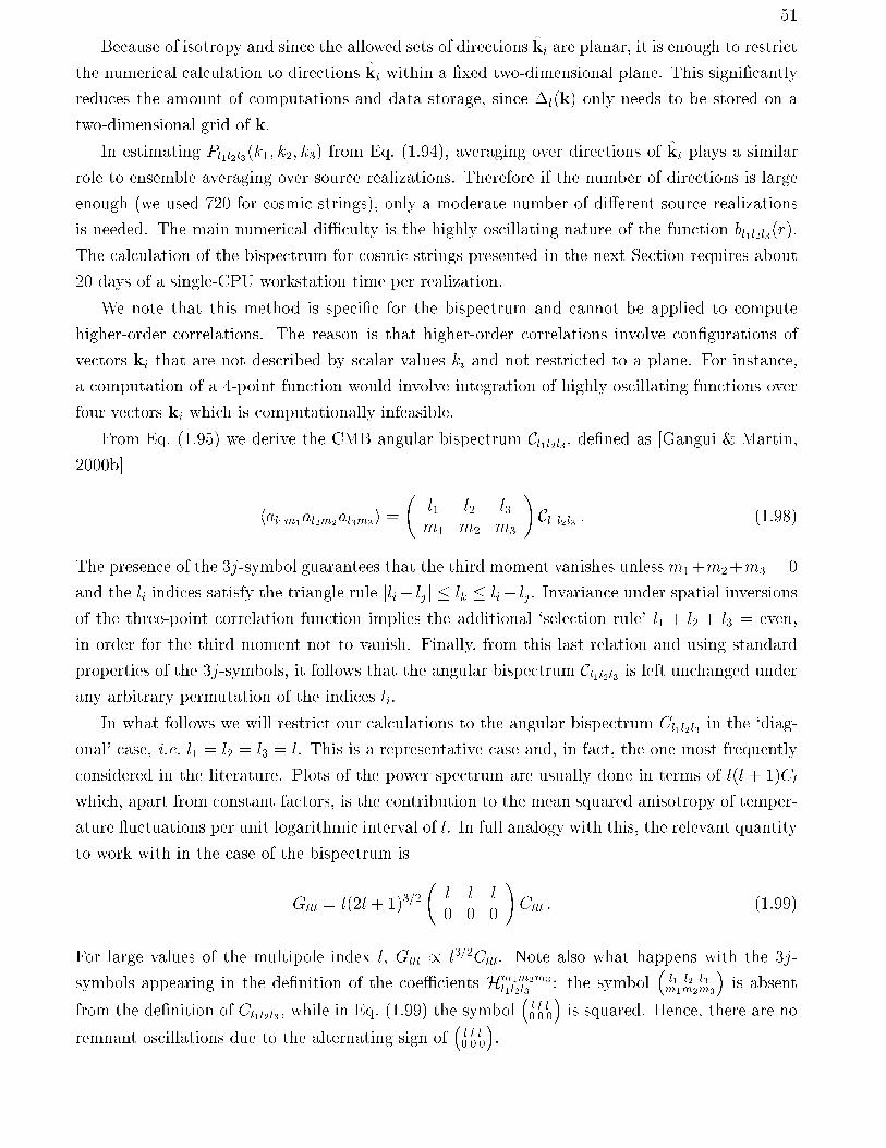
51

Because of isotropy and since the allowed sets of directions ki are planar, it is enough to restrict

the numerical calculation to directions ki within a xed two-dimensional plane. This signicantly

reduces the amount of computations and data storage, since l(k) only needs to be stored on a

two-dimensional grid of k.

In estimating Pl1l2l3(k1; k2; k3) from Eq. (1.94), averaging over directions of ki plays a similar

role to ensemble averaging over source realizations. Therefore if the number of directions is large

enough (we used 720 for cosmic strings), only a moderate number of dierent source realizations

is needed. The main numerical diÆculty is the highly oscillating nature of the function bl1l2l3(r).

The calculation of the bispectrum for cosmic strings presented in the next Section requires about

20 days of a single-CPU workstation time per realization.

We note that this method is specic for the bispectrum and cannot be applied to compute

higher-order correlations. The reason is that higher-order correlations involve congurations of

vectors ki that are not described by scalar values ki and not restricted to a plane. For instance,

a computation of a 4-point function would involve integration of highly oscillating functions over

four vectors ki which is computationally infeasible.

From Eq. (1.95) we derive the CMB angular bispectrum Cl1l2l3, dened as [Gangui & Martin,

2000b]

hal1m1al2m2

al3m3i =

l1 l2 l3m1 m2 m3

!Cl1l2l3 : (1.98)

The presence of the 3j-symbol guarantees that the third moment vanishes unless m1+m2+m3 = 0

and the li indices satisfy the triangle rule jli ljj lk li+ lj. Invariance under spatial inversions

of the three-point correlation function implies the additional `selection rule' l1 + l2 + l3 = even,

in order for the third moment not to vanish. Finally, from this last relation and using standard

properties of the 3j-symbols, it follows that the angular bispectrum Cl1l2l3 is left unchanged under

any arbitrary permutation of the indices li.

In what follows we will restrict our calculations to the angular bispectrum Cl1l2l3 in the `diag-

onal' case, i.e. l1 = l2 = l3 = l. This is a representative case and, in fact, the one most frequently

considered in the literature. Plots of the power spectrum are usually done in terms of l(l + 1)Cl

which, apart from constant factors, is the contribution to the mean squared anisotropy of temper-

ature uctuations per unit logarithmic interval of l. In full analogy with this, the relevant quantity

to work with in the case of the bispectrum is

Glll = l(2l + 1)3=2 l l l0 0 0

!Clll : (1.99)

For large values of the multipole index l, Glll / l3=2Clll. Note also what happens with the 3j-

symbols appearing in the denition of the coeÆcients Hm1m2m3

l1l2l3: the symbol

l1 l2 l3m1m2m3

is absent

from the denition of Cl1l2l3 , while in Eq. (1.99) the symboll l l0 0 0

is squared. Hence, there are no

remnant oscillations due to the alternating sign ofl l l0 0 0

.

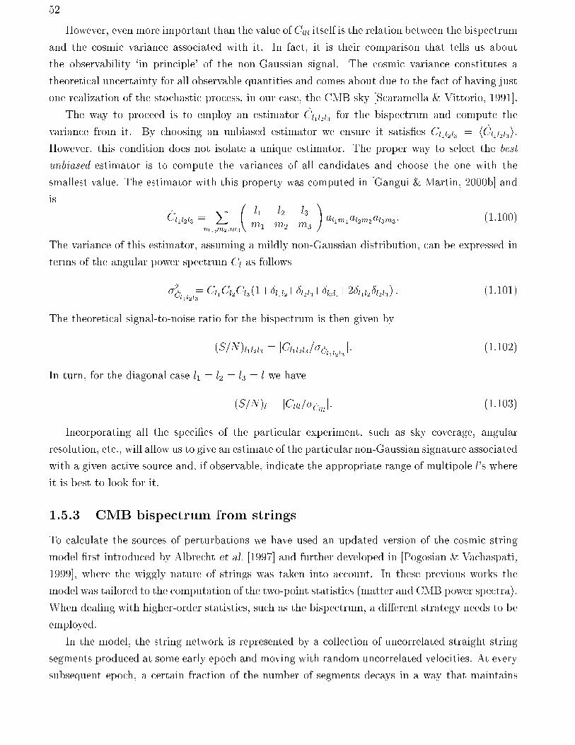
52

However, even more important than the value of Clll itself is the relation between the bispectrum

and the cosmic variance associated with it. In fact, it is their comparison that tells us about

the observability `in principle' of the non-Gaussian signal. The cosmic variance constitutes a

theoretical uncertainty for all observable quantities and comes about due to the fact of having just

one realization of the stochastic process, in our case, the CMB sky [Scaramella & Vittorio, 1991].

The way to proceed is to employ an estimator Cl1l2l3 for the bispectrum and compute the

variance from it. By choosing an unbiased estimator we ensure it satises Cl1l2l3 = hCl1l2l3i.However, this condition does not isolate a unique estimator. The proper way to select the best

unbiased estimator is to compute the variances of all candidates and choose the one with the

smallest value. The estimator with this property was computed in [Gangui & Martin, 2000b] and

is

Cl1l2l3 =X

m1;m2;m3

l1 l2 l3m1 m2 m3

!al1m1

al2m2al3m3

: (1.100)

The variance of this estimator, assuming a mildly non-Gaussian distribution, can be expressed in

terms of the angular power spectrum Cl as follows

2Cl1l2l3

= Cl1Cl2Cl3(1+Æl1l2+Æl2l3+Æl3l1+2Æl1l2Æl2l3) : (1.101)

The theoretical signal-to-noise ratio for the bispectrum is then given by

(S=N)l1l2l3 = jCl1l2l3=Cl1l2l3j: (1.102)

In turn, for the diagonal case l1 = l2 = l3 = l we have

(S=N)l = jClll=Clllj: (1.103)

Incorporating all the specics of the particular experiment, such as sky coverage, angular

resolution, etc., will allow us to give an estimate of the particular non-Gaussian signature associated

with a given active source and, if observable, indicate the appropriate range of multipole l's where

it is best to look for it.

1.5.3 CMB bispectrum from strings

To calculate the sources of perturbations we have used an updated version of the cosmic string

model rst introduced by Albrecht et al. [1997] and further developed in [Pogosian & Vachaspati,

1999], where the wiggly nature of strings was taken into account. In these previous works the

model was tailored to the computation of the two-point statistics (matter and CMB power spectra).

When dealing with higher-order statistics, such as the bispectrum, a dierent strategy needs to be

employed.

In the model, the string network is represented by a collection of uncorrelated straight string

segments produced at some early epoch and moving with random uncorrelated velocities. At every

subsequent epoch, a certain fraction of the number of segments decays in a way that maintains

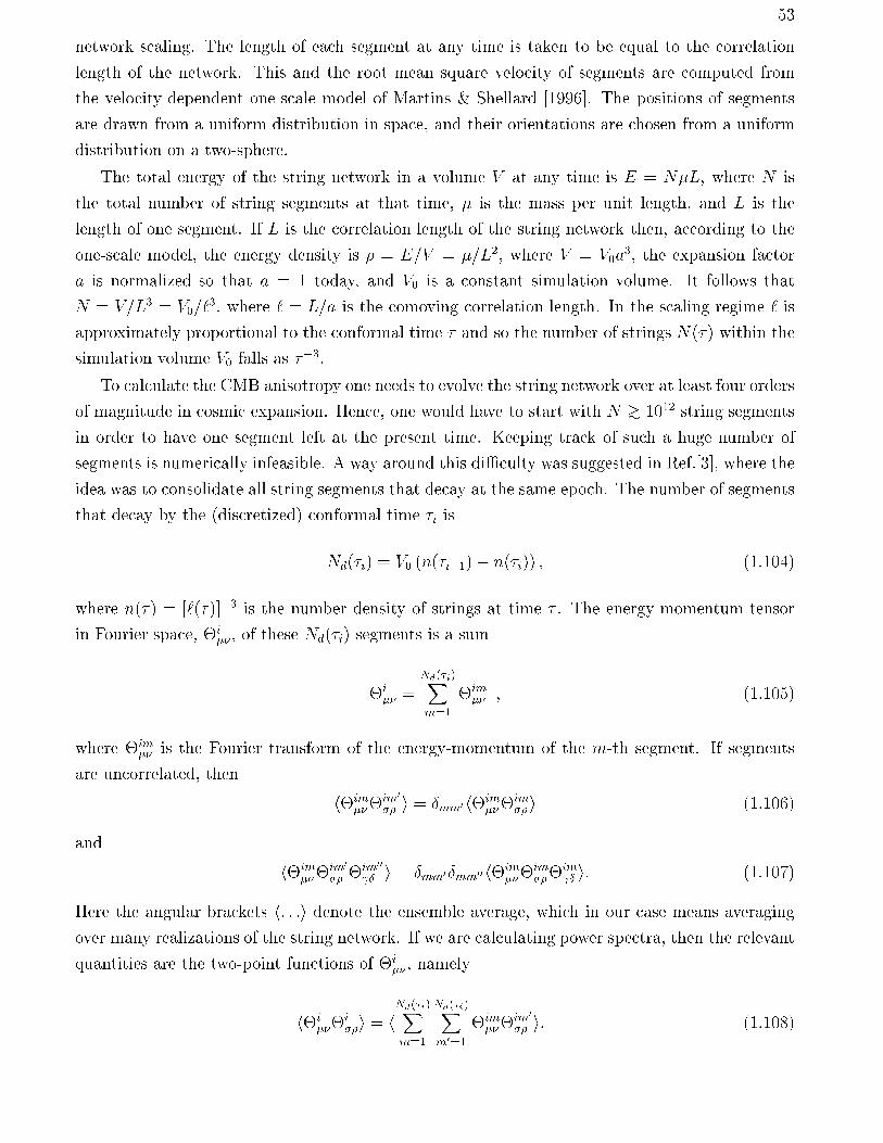
53

network scaling. The length of each segment at any time is taken to be equal to the correlation

length of the network. This and the root mean square velocity of segments are computed from

the velocity-dependent one-scale model of Martins & Shellard [1996]. The positions of segments

are drawn from a uniform distribution in space, and their orientations are chosen from a uniform

distribution on a two-sphere.

The total energy of the string network in a volume V at any time is E = NL, where N is

the total number of string segments at that time, is the mass per unit length, and L is the

length of one segment. If L is the correlation length of the string network then, according to the

one-scale model, the energy density is = E=V = =L2, where V = V0a3, the expansion factor

a is normalized so that a = 1 today, and V0 is a constant simulation volume. It follows that

N = V=L3 = V0=`3, where ` = L=a is the comoving correlation length. In the scaling regime ` is

approximately proportional to the conformal time and so the number of strings N() within the

simulation volume V0 falls as 3.

To calculate the CMB anisotropy one needs to evolve the string network over at least four orders

of magnitude in cosmic expansion. Hence, one would have to start with N > 1012 string segments

in order to have one segment left at the present time. Keeping track of such a huge number of

segments is numerically infeasible. A way around this diÆculty was suggested in Ref.[3], where the

idea was to consolidate all string segments that decay at the same epoch. The number of segments

that decay by the (discretized) conformal time i is

Nd(i) = V0 (n(i1) n(i)) ; (1.104)

where n() = [`()]3 is the number density of strings at time . The energy-momentum tensor

in Fourier space, i, of these Nd(i) segments is a sum

i =

Nd(i)Xm=1

im ; (1.105)

where im is the Fourier transform of the energy-momentum of the m-th segment. If segments

are uncorrelated, then

him

im0

i = Æmm0him

im i (1.106)

and

him

im0

im00

Æ i = Æmm0Æmm00him

im

im Æ i: (1.107)

Here the angular brackets h: : :i denote the ensemble average, which in our case means averaging

over many realizations of the string network. If we are calculating power spectra, then the relevant

quantities are the two-point functions of i, namely

hi

ii = h

Nd(i)Xm=1

Nd(i)Xm0=1

im

im0

i: (1.108)

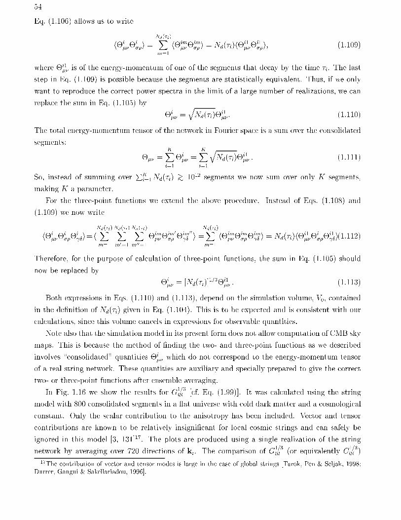
54

Eq. (1.106) allows us to write

hi

ii =

Nd(i)Xm=1

him

im i = Nd(i)hi1

i1i; (1.109)

where i1 is of the energy-momentum of one of the segments that decay by the time i. The last

step in Eq. (1.109) is possible because the segments are statistically equivalent. Thus, if we only

want to reproduce the correct power spectra in the limit of a large number of realizations, we can

replace the sum in Eq. (1.105) by

i =

qNd(i)

i1: (1.110)

The total energy-momentum tensor of the network in Fourier space is a sum over the consolidated

segments:

=KXi=1

i =

KXi=1

qNd(i)

i1 : (1.111)

So, instead of summing overPK

i=1Nd(i) > 1012 segments we now sum over only K segments,

making K a parameter.

For the three-point functions we extend the above procedure. Instead of Eqs. (1.108) and

(1.109) we now write

hi

i

i Æi=h

Nd(i)Xm=1

Nd(i)Xm0=1

Nd(i)Xm00=1

im

im0

im00

Æ i =Nd(i)Xm=1

him

im

im Æ i = Nd(i)hi1

i1

i1 Æi(1.112)

Therefore, for the purpose of calculation of three-point functions, the sum in Eq. (1.105) should

now be replaced by

i = [Nd(i)]

1=3i1 : (1.113)

Both expressions in Eqs. (1.110) and (1.113), depend on the simulation volume, V0, contained

in the denition of Nd(i) given in Eq. (1.104). This is to be expected and is consistent with our

calculations, since this volume cancels in expressions for observable quantities.

Note also that the simulation model in its present form does not allow computation of CMB sky

maps. This is because the method of nding the two- and three-point functions as we described

involves \consolidated" quantities i which do not correspond to the energy-momentum tensor

of a real string network. These quantities are auxiliary and specially prepared to give the correct

two- or three-point functions after ensemble averaging.

In Fig. 1.16 we show the results for G1=3lll [cf. Eq. (1.99)]. It was calculated using the string

model with 800 consolidated segments in a at universe with cold dark matter and a cosmological

constant. Only the scalar contribution to the anisotropy has been included. Vector and tensor

contributions are known to be relatively insignicant for local cosmic strings and can safely be

ignored in this model [3, 131]17. The plots are produced using a single realization of the string

network by averaging over 720 directions of ki. The comparison of G1=3lll (or equivalently C

1=3lll )

17The contribution of vector and tensor modes is large in the case of global strings [Turok, Pen & Seljak, 1998;Durrer, Gangui & Sakellariadou, 1996].

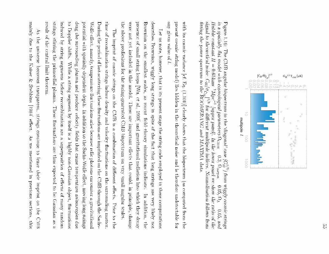
55

multipole l

Glll1/3 T

CMB[mK]Clll

Clll1/3

s^/| |

Figu

re1.16:

TheCMBangular

bisp

ectrum

inthe`diagon

al'case

(G1=3

lll)from

wiggly

cosmicstrin

gsin

aspatially

at

modelwith

cosmological

param

etersCDM=0:3,

baryon=0:05,

=0:65,

and

Hubblecon

stantH

=0:65k

ms1M

pc1[upper

panel].

Inthelow

erpanelweshow

theratio

ofthe

signal

totheoretical

noisejC

lll =C

lll j 1=3for

dieren

tmultip

oleindices.

Norm

alizationfollow

sfrom

ttin

gthepow

erspectru

mto

theBOOMERANG

andMAXIM

Adata.

with

itscosm

icvarian

ce[cf.

Eq.(1.101)]

clearlyshow

sthat

thebisp

ectrum

(ascom

puted

fromthe

presen

tcosm

icstrin

gmodel)

lieshidden

inthetheoretical

noise

andistherefore

undetectab

lefor

anygiven

valueofl.

Let

usnote,

how

ever,that

inits

presen

tstage

thestrin

gcodeem

ployed

inthese

computation

s

describ

esBrow

nian

,wiggly

longstrin

gsin

spite

ofthefact

that

longstrin

gsare

verylikely

not

Brow

nian

onthesm

allestscales,

asrecen

teld

theory

simulation

sindicate.

Inaddition

,the

presen

ceof

small

stringloops[W

u,et

al.,1998]

andgrav

itationalrad

iationinto

which

they

decay

were

not

yetinclu

ded

inthismodel.

These

areim

portan

teects

that

could,in

prin

ciple,

change

theabove

pred

ictionsfor

thestrin

g-generated

CMBbisp

ectrum

onvery

small

angular

scales.

Theim

prin

tof

cosmicstrin

gson

theCMBisacom

bination

ofdieren

teects.

Prior

tothe

timeof

recombination

strings

induce

density

andvelo

city uctu

ationson

thesurrou

ndingmatter.

Durin

gtheperio

doflast

scatteringthese

uctu

ationsare

imprin

tedon

theCMBthrou

ghtheSach

s-

Wolfe

eect,

nam

ely,tem

peratu

re uctu

ationsarise

becau

serelic

photon

sencou

nter

agrav

itational

poten

tialwith

spatially

dependentdepth.In

addition

totheSach

s-Wolfe

eect,

movinglon

gstrin

gs

drag

thesurrou

ndingplasm

aandproduce

velocity

eld

sthat

cause

temperatu

reanisotrop

iesdue

toDoppler

shifts.

While

astrin

gsegm

entbyitself

isahigh

lynon-G

aussian

object,

uctu

ations

induced

bystrin

gsegm

ents

before

recombination

areasuperp

ositionof

eects

ofmanyran

dom

strings

stirringtheprim

ordial

plasm

a.These

uctu

ationsare

thusexpected

tobeGaussian

asa

resultof

thecen

trallim

ittheorem

.

Astheuniverse

becom

estran

sparen

t,strin

gscon

tinueto

leavetheir

imprin

ton

theCMB

main

lydueto

theKaiser

&Steb

bins[1984]

eect.

Aswemention

edin

prev

ioussection

s,this

56

eect results in line discontinuities in the temperature eld of photons passing on opposite sides

of a moving long string.18 However, this eect can result in non-Gaussian perturbations only

on suÆciently small scales. This is because on scales larger than the characteristic inter-string

separation at the time of the radiation-matter equality, the CMB temperature perturbations result

from superposition of eects of many strings and are likely to be Gaussian. Avelino et al. [1998]

applied several non-Gaussian tests to the perturbations seeded by cosmic strings. They found the

density eld distribution to be close to Gaussian on scales larger than 1:5(Mh2)1 Mpc, where

M is the fraction of cosmological matter density in baryons and CDM combined. Scales this

small correspond to the multipole index of order l 104.

1.5.4 CMB polarization

The possibility that the CMB be polarized was rst discussed by Martin Rees in 1968, in the context

of anisotropic Universe models. In spite of his optimism, and after more than thirty years, there is

still no positive detection of the polarization eld. Unlike the BOOMERANG[G experiment,

MAP will have the capability to detect it and this to a level of better than 10 K in its low frequency

channels. Polarization is an important probe both for cosmological models and for the more recent

history of our nearby Universe. It arises from the interactions of CMB photons with free electrons;

hence, polarization can only be produced at the last scattering surface (its amplitude depends on

the duration of the decoupling process) and, unlike temperature uctuations, it is unaected by

variations of the gravitational potential after last scattering. Future measurements of polarization

will thus provide a clean view of the inhomogeneities of the Universe at about 400,000 years after

the Bang.

For understanding polarization, a couple of things should be clear. First, the energy of the

photons is small compared to the mass of the electrons. Then, the CMB frequency does not

change, since the electron recoil is negligible. Second, the change in the CMB polarization (i.e.,

the orientation of the oscillating electric eld ~E of the radiation) occurs due to a certain transition,

called Thomson scattering. The transition probability per unit time is proportional to a combina-

tion of the old ( in ) and new ( out

) directions of polarization in the form j in out

j2. In other

words, the initial direction of polarization will be favored. Third, an oscillating ~E will push the

electron to also oscillate; the latter can then be seen as a dipole (not to be confused with the CMB

dipole), and dipole radiation emits preferentially perpendicularly to the direction of oscillation.

These `rules' will help us understand why the CMB should be linearly polarized.

Previous to the recombination epoch, the radiation eld is unpolarized. In unpolarized light

the electric eld can be decomposed into the two orthogonal directions (along, say, x and z)

perpendicular to the line of propagation (y). The electric eld along inz (suppose z is vertical)

will make the electron oscillate also vertically. Hence, the dipolar radiation will be maximal over

18The extension of the Kaiser-Stebbins eect to polarization will be treated below. In fact, Benabed andBernardeau [2000] have recently considered the generation of a B-type polarization eld out of E-type polarization,through gravitational lensing on a cosmic string.

57

the horizontal xy-plane. Analogously, dipole radiation due to the electric eld along x will be on the

yz-plane. If we now look from the side (e.g., from x, on the horizontal plane and perpendicularly

to the incident direction y) we will see a special kind of scattered radiation. From our position we

cannot perceive the radiation that the electron oscillating along the x direction would emit, just

because this radiation goes to the yz-plane, orthogonal to us. Then, it is as if only the vertical

component ( inz ) of the incoming electric eld would cause the radiation we perceive. From the

above rules we know that the highest probability for the polarization of the outgoing radiation

out will be to be aligned with the incoming one in

z , and therefore it follows that the outgoing

radiation will be linearly polarized. Now, as both the chosen incoming direction and our position

as observers were arbitrary, the result will not be modied if we change them. Thomson scattering

will convert unpolarized radiation into linearly polarized one.

This however is not the end of the story. To get the total eect we need to consider all possible

directions from which photons will come to interact with the target electron, and sum them up.

We see easily that for an initial isotropic radiation distribution the individual contributions will

cancel out: just from symmetry arguments, in a spherically symmetric conguration no direction is

privileged, unlike the case of a net linear polarization which would select one particular direction.

Fortunately, we know the CMB is not exactly isotropic; to the millikelvin precision the dominant

mode is dipolar. So, what about a CMB dipolar distribution ? Although spatial symmetry does

not help us now, a dipole will not generate polarization either. Take, for example, the radiation

incident onto the electron from the left to be more intense than the radiation incident from the

right, with average intensities above and below (that's a dipole); it then suÆces to sum up all

contributions to see that no net polarization survives. However, if the CMB has a quadrupolar

variation in temperature (that it has, rst discovered by COBE, to tens of K precision) then there

will be an excess of vertical polarization from left- and right-incident photons (assumed hotter than

the mean) with respect to the horizontal one from top and bottom light (cooler). From any point

of view, orthogonal contributions to the nal polarization will be dierent, leaving a net linear

polarization in the scattered radiation.

Within standard recombination models the predicted level of linear polarization on large scales

is tiny (see Figure 1.17): the quadrupole generated in the radiation distribution as the photons

travel between successive scatterings is too small. Multiple scatterings make the plasma very

homogeneous and only wavelengths that are small enough (big `'s) to produce anisotropies over

the (rather short) mean free path of the photons will lead to a signicant quadrupole, and thus

also to polarization. Indeed, if the CMB photons last scattered at z 1100, the SCDM model

with h = 1 predicts no more than 0.05 K on scales greater than a few degrees. Hence, measuring

polarization represents an experimental challenge. There is still no positive detection and the best

upper limits a few years ago were around 25K, obtained by Edward Wollack and collaborators in

1993, and now improved to roughly 10K on subdegree angular scales by Hedman, et al., [2000]19.

19They actually nd upper limits of 14K and 13K on the amplitudes of the E and B modes, respectively, ofthe polarization eld more below. And, if in their analysis they assumed there are no B modes, then the limit on

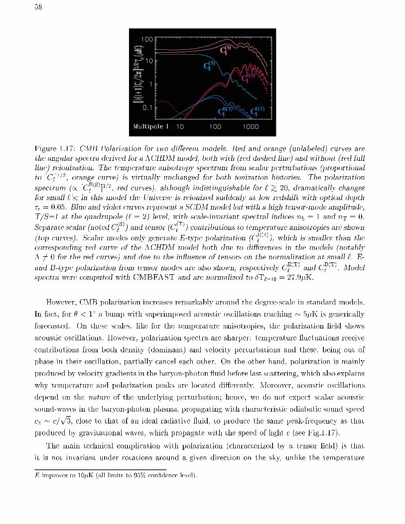
58

E(S)Cl

(S)Cl

E(T)Cl

(T)Cl

B(T)Cl

Figure 1.17: CMB Polarization for two dierent models. Red and orange (unlabeled) curves arethe angular spectra derived for a CHDM model, both with (red dashed line) and without (red fullline) reionization. The temperature anisotropy spectrum from scalar perturbations (proportionalto [C`]

1=2, orange curve) is virtually unchanged for both ionization histories. The polarization

spectrum (/ [CE(S)` ]1=2, red curves), although indistinguishable for ` > 20, dramatically changes

for small `'s; in this model the Universe is reionized suddenly at low redshift with optical depthc = 0:05. Blue and violet curves represent a SCDM model but with a high tensor-mode amplitude,T/S=1 at the quadrupole (` = 2) level, with scale-invariant spectral indices nS = 1 and nT = 0.

Separate scalar (noted C(S)` ) and tensor (C

(T)` ) contributions to temperature anisotropies are shown

(top curves). Scalar modes only generate E-type polarization (CE(S)` ), which is smaller than the

corresponding red curve of the CHDM model both due to dierences in the models (notably 6= 0 for the red curves) and due to the in uence of tensors on the normalization at small `. E-

and B-type polarization from tensor modes are also shown, respectively CE(T)` and C

B(T)` . Model

spectra were computed with CMBFAST and are normalized to ÆT`=10 = 27:9K.

However, CMB polarization increases remarkably around the degree-scale in standard models.

In fact, for < 1Æ a bump with superimposed acoustic oscillations reaching 5K is generically

forecasted. On these scales, like for the temperature anisotropies, the polarization eld shows

acoustic oscillations. However, polarization spectra are sharper: temperature uctuations receive

contributions from both density (dominant) and velocity perturbations and these, being out of

phase in their oscillation, partially cancel each other. On the other hand, polarization is mainly

produced by velocity gradients in the baryon-photon uid before last scattering, which also explains

why temperature and polarization peaks are located dierently. Moreover, acoustic oscillations

depend on the nature of the underlying perturbation; hence, we do not expect scalar acoustic

sound-waves in the baryon-photon plasma, propagating with characteristic adiabatic sound speed

cS c=p3, close to that of an ideal radiative uid, to produce the same peak-frequency as that

produced by gravitational waves, which propagate with the speed of light c (see Fig.1.17).

The main technical complication with polarization (characterized by a tensor eld) is that

it is not invariant under rotations around a given direction on the sky, unlike the temperature

E improves to 10K (all limits to 95% condence level).

59

uctuation that is described by a scalar quantity and invariant under such rotations. The level of

linear polarization is conveniently expressed in terms of the Stokes parametersQ and U. It turns out

that there is a clever combination of these parameters that results in scalar quantities (in contrast

to the above noninvariant tensor description) but with dierent transformation properties under

spatial inversions (parity transformations). Then, inspired by classical electromagnetism, any

polarization pattern on the sky can be separated into `electric' (scalar, unchanged under parity

transformation) and `magnetic' (pseudo-scalar, changes sign under parity) components (E- and

B-type polarization, respectively).

CMB polarization from global defects

One then expands these dierent components in terms of spherical harmonics, very much like

we did for temperature anisotropies, getting coeÆcients am` for E and B polarizations and, from

these, the multipoles CE;B` . The interesting thing is that (for symmetry reasons) scalar-density

perturbations will not produce any B polarization (a pseudo-scalar), that is CB(S)` = 0. We see

then that an unambiguous detection of some level of B-type uctuations will be a signature of the

existence (and of the amplitude) of a background of gravitational waves ! [Seljak & Zaldarriaga,

1997] (and, if present, also of rotational modes, like in models with topological defects).

Linear polarization is a symmetric and traceless 2x2 tensor that requires 2 parameters to fully

describe it: Q, U Stokes parameters. These depend on the orientation of the coordinate system

on the sky. It is convenient to use Q + iU and Q iU as the two independent combinations,

which transform under right-handed rotation by an angle as (Q + iU)0 = e2i(Q + iU) and

(Q iU)0 = e2i(Q iU). These two quantities have spin-weights 2 and 2 respectively and can

be decomposed into spin 2 spherical harmonics 2Ylm

(Q + iU)(n) =Xlm

a2;lm 2Ylm(n) (1.114)

(Q iU)(n) =Xlm

a2;lm 2Ylm(n): (1.115)

Spin s spherical harmonics form a complete orthonormal system for each value of s. Important

property of spin-weighted basis: there exists spin raising and lowering operators 0@ and 0@ . By

acting twice with a spin lowering and raising operator on (Q+ iU) and (Q iU) respectively one

obtains quantities of spin 0, which are rotationally invariant. These quantities can be treated like

the temperature and no ambiguities connected with the orientation of coordinate system on the

sky will arise. Conversely, by acting with spin lowering and raising operators on usual harmonics

spin s harmonics can be written explicitly in terms of derivatives of the usual spherical harmonics.

Their action on 2Ylm leads to

0@ 2(Q+ iU)(n) =Xlm

[l + 2]!

[l 2]!

!1=2

a2;lmYlm(n) (1.116)

60

0@ 2(Q iU)(n) =Xlm

[l + 2]!

[l 2]!

!1=2

a2;lmYlm(n): (1.117)

With these denitions the expressions for the expansion coeÆcients of the two polarization variables

become [Seljak & Zaldarriaga, 1997]

a2;lm =

[l 2]!

[l + 2]!

!1=2 Zd Y

lm(n)0@ 2(Q+ iU)(n) (1.118)

a2;lm =

[l 2]!

[l + 2]!

!1=2 Zd Y

lm(n)0@ 2(Q iU)(n): (1.119)

Instead of a2;lm, a2;lm it is convenient to introduce their linear electric and magnetic combinations

aE;lm = 12(a2;lm + a2;lm) aB;lm =

i

2(a2;lm a2;lm): (1.120)

These two behave dierently under parity transformation: while E remains unchanged B changes

the sign, in analogy with electric and magnetic elds.

To characterize the statistics of the CMB perturbations only four power spectra are needed,

those for X = T;E;B and the cross correlation between T and E. The cross correlation between

B and E or B and T vanishes because B has the opposite parity of T and E. As usual, the spectra

are dened as the rotationally invariant quantities

CXl =1

2l + 1

Xm

haX;lmaX;lmi CCl =1

2l + 1

Xm

haT;lmaE;lmi (1.121)

in terms of which on has

haX;l0m0aX;lmi = CXl Æl0lÆm0m (1.122)

haT;l0m0aE;lmi = CCl Æl0lÆm0m (1.123)

haB;l0m0aE;lmi = haB;l0m0aT;lmi = 0: (1.124)

According to what was said above, one expects some amount of polarization to be present in

all possible cosmological models. However, symmetry breaking models giving rise to topological

defects dier from in ationary models in several important aspects, two of which are the relative

contributions from scalar, vector and tensor modes and the coherence of the seeds sourcing the

perturbation equations. In the local cosmic string case one nds that in general scalar modes are

dominant, if one compares to vector and tensor modes in the usual decomposition of perturbations.

The situation with global topological defects is radically dierent and this leads to a very distinctive

signature in the polarization eld.

Temperature and polarization spectra for various symmetry breaking models were calculated

by Seljak, Pen & Turok [1997] and are shown in gure 1.18. Both electric and magnetic compo-

nents of polarization are shown for a variety of global defects. They also plot for comparison the

corresponding spectra in a typical in ationary model, namely, the standard CDM model (h = 0:5,

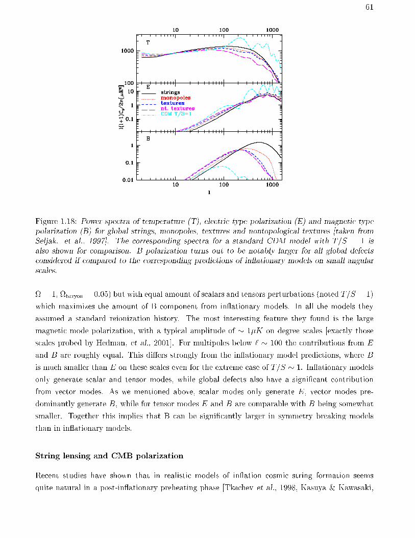
61

Figure 1.18: Power spectra of temperature (T), electric type polarization (E) and magnetic typepolarization (B) for global strings, monopoles, textures and nontopological textures [taken fromSeljak. et al., 1997]. The corresponding spectra for a standard CDM model with T=S = 1 isalso shown for comparison. B polarization turns out to be notably larger for all global defectsconsidered if compared to the corresponding predictions of in ationary models on small angularscales.

= 1, baryon = 0:05) but with equal amount of scalars and tensors perturbations (noted T=S = 1)

which maximizes the amount of B component from in ationary models. In all the models they

assumed a standard reionization history. The most interesting feature they found is the large

magnetic mode polarization, with a typical amplitude of 1K on degree scales [exactly those

scales probed by Hedman, et al., 2001]. For multipoles below ` 100 the contributions from E

and B are roughly equal. This diers strongly from the in ationary model predictions, where B

is much smaller than E on these scales even for the extreme case of T=S 1. In ationary models

only generate scalar and tensor modes, while global defects also have a signicant contribution

from vector modes. As we mentioned above, scalar modes only generate E, vector modes pre-

dominantly generate B, while for tensor modes E and B are comparable with B being somewhat

smaller. Together this implies that B can be signicantly larger in symmetry breaking models

than in in ationary models.

String lensing and CMB polarization

Recent studies have shown that in realistic models of in ation cosmic string formation seems

quite natural in a post-in ationary preheating phase [Tkachev et al., 1998, Kasuya & Kawasaki,

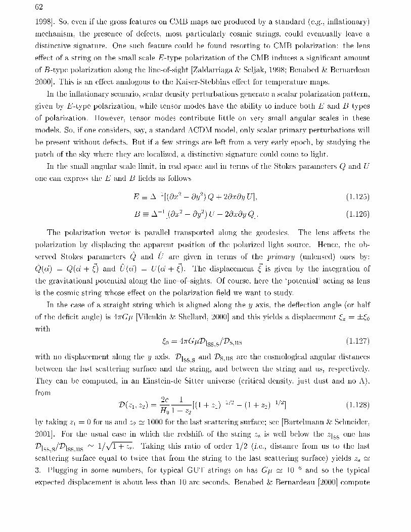
62

1998]. So, even if the gross features on CMB maps are produced by a standard (e.g., in ationary)

mechanism, the presence of defects, most particularly cosmic strings, could eventually leave a

distinctive signature. One such feature could be found resorting to CMB polarization: the lens

eect of a string on the small scale E-type polarization of the CMB induces a signicant amount

of B-type polarization along the line-of-sight [Zaldarriaga & Seljak, 1998; Benabed & Bernardeau

2000]. This is an eect analogous to the Kaiser-Stebbins eect for temperature maps.

In the in ationary scenario, scalar density perturbations generate a scalar polarization pattern,

given by E-type polarization, while tensor modes have the ability to induce both E and B types

of polarization. However, tensor modes contribute little on very small angular scales in these

models. So, if one considers, say, a standard CDM model, only scalar primary perturbations will

be present without defects. But if a few strings are left from a very early epoch, by studying the

patch of the sky where they are localized, a distinctive signature could come to light.

In the small angular scale limit, in real space and in terms of the Stokes parameters Q and U

one can express the E and B elds as follows

E 1[(@x2 @y2)Q+ 2@x@y U ]; (1.125)

B 1[(@x2 @y2)U 2@x@y Q]: (1.126)

The polarization vector is parallel transported along the geodesics. The lens aects the

polarization by displacing the apparent position of the polarized light source. Hence, the ob-

served Stokes parameters Q and U are given in terms of the primary (unlensed) ones by:

Q(~) = Q(~ + ~) and U(~) = U(~ + ~). The displacement ~ is given by the integration of

the gravitational potential along the lineofsights. Of course, here the `potential' acting as lens

is the cosmic string whose eect on the polarization eld we want to study.

In the case of a straight string which is aligned along the y axis, the de ection angle (or half

of the decit angle) is 4G [Vilenkin & Shellard, 2000] and this yields a displacement x = 0with

0 = 4GDlss,s=Ds,us (1.127)

with no displacement along the y axis. Dlss,s and Ds,us are the cosmological angular distances

between the last scattering surface and the string, and between the string and us, respectively.

They can be computed, in an Einstein-de Sitter universe (critical density, just dust and no ),

from

D(z1; z2) = 2c

H0

1

1 + z2[(1 + z1)

1=2 (1 + z2)1=2] (1.128)

by taking z1 = 0 for us and z2 ' 1000 for the last scattering surface; see [Bartelmann & Schneider,

2001]. For the usual case in which the redshift of the string zs is well below the zlss one has

Dlss,s=Dlss,us ' 1=p1 + zs. Taking this ratio of order 1/2 (i.e., distance from us to the last

scattering surface equal to twice that from the string to the last scattering surface) yields zs '3. Plugging in some numbers, for typical GUT strings on has G ' 106 and so the typical

expected displacement is about less than 10 arc seconds. Benabed & Bernardeau [2000] compute

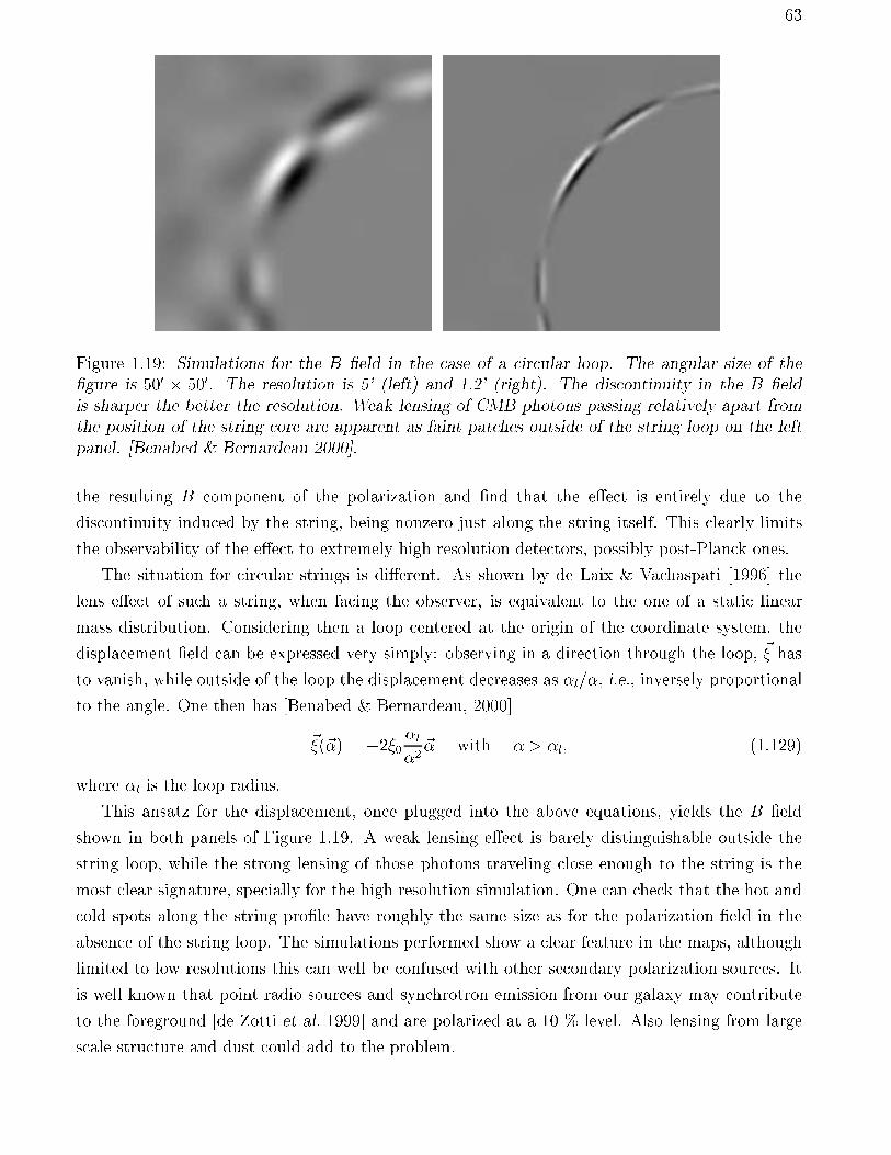
63

Figure 1.19: Simulations for the B eld in the case of a circular loop. The angular size of thegure is 500 500. The resolution is 5' (left) and 1.2' (right). The discontinuity in the B eldis sharper the better the resolution. Weak lensing of CMB photons passing relatively apart fromthe position of the string core are apparent as faint patches outside of the string loop on the leftpanel. [Benabed & Bernardeau 2000].

the resulting B component of the polarization and nd that the eect is entirely due to the

discontinuity induced by the string, being nonzero just along the string itself. This clearly limits

the observability of the eect to extremely high resolution detectors, possibly post-Planck ones.

The situation for circular strings is dierent. As shown by de Laix & Vachaspati [1996] the

lens eect of such a string, when facing the observer, is equivalent to the one of a static linear

mass distribution. Considering then a loop centered at the origin of the coordinate system, the

displacement eld can be expressed very simply: observing in a direction through the loop, ~ has

to vanish, while outside of the loop the displacement decreases as l=, i.e., inversely proportional

to the angle. One then has [Benabed & Bernardeau, 2000]

~(~) = 20 l2~ with > l; (1.129)

where l is the loop radius.

This ansatz for the displacement, once plugged into the above equations, yields the B eld

shown in both panels of Figure 1.19. A weak lensing eect is barely distinguishable outside the

string loop, while the strong lensing of those photons traveling close enough to the string is the

most clear signature, specially for the high resolution simulation. One can check that the hot and

cold spots along the string prole have roughly the same size as for the polarization eld in the

absence of the string loop. The simulations performed show a clear feature in the maps, although

limited to low resolutions this can well be confused with other secondary polarization sources. It

is well known that point radio sources and synchrotron emission from our galaxy may contribute

to the foreground [de Zotti et al. 1999] and are polarized at a 10 % level. Also lensing from large

scale structure and dust could add to the problem.

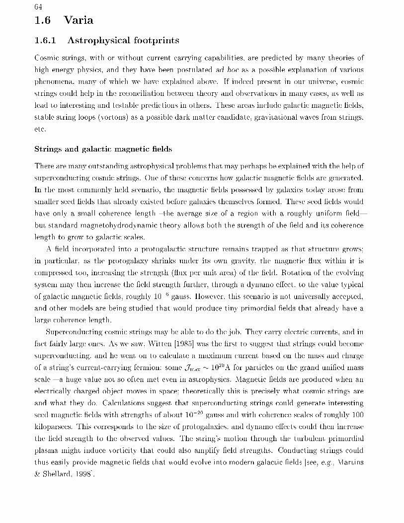
64

1.6 Varia

1.6.1 Astrophysical footprints

Cosmic strings, with or without current carrying capabilities, are predicted by many theories of

high energy physics, and they have been postulated ad hoc as a possible explanation of various

phenomena, many of which we have explained above. If indeed present in our universe, cosmic

strings could help in the reconciliation between theory and observations in many cases, as well as

lead to interesting and testable predictions in others. These areas include galactic magnetic elds,

stable string loops (vortons) as a possible dark matter candidate, gravitational waves from strings,

etc.

Strings and galactic magnetic elds

There are many outstanding astrophysical problems that may perhaps be explained with the help of

superconducting cosmic strings. One of these concerns how galactic magnetic elds are generated.

In the most commonly held scenario, the magnetic elds possessed by galaxies today arose from

smaller seed elds that already existed before galaxies themselves formed. These seed elds would

have only a small coherence length the average size of a region with a roughly uniform eld

but standard magnetohydrodynamic theory allows both the strength of the eld and its coherence

length to grow to galactic scales.

A eld incorporated into a protogalactic structure remains trapped as that structure grows;

in particular, as the protogalaxy shrinks under its own gravity, the magnetic ux within it is

compressed too, increasing the strength ( ux per unit area) of the eld. Rotation of the evolving

system may then increase the eld strength further, through a dynamo eect, to the value typical

of galactic magnetic elds, roughly 106 gauss. However, this scenario is not universally accepted,

and other models are being studied that would produce tiny primordial elds that already have a

large coherence length.

Superconducting cosmic strings may be able to do the job. They carry electric currents, and in

fact fairly large ones. As we saw, Witten [1985] was the rst to suggest that strings could become

superconducting, and he went on to calculate a maximum current based on the mass and charge

of a string's current-carrying fermion: some Jmax 1020A for particles on the grand unied mass

scale a huge value not so often met even in astrophysics. Magnetic elds are produced when an

electrically charged object moves in space; theoretically this is precisely what cosmic strings are

and what they do. Calculations suggest that superconducting strings could generate interesting

seed magnetic elds with strengths of about 1020 gauss and with coherence scales of roughly 100

kiloparsecs. This corresponds to the size of protogalaxies, and dynamo eects could then increase

the eld strength to the observed values. The string's motion through the turbulent primordial

plasma might induce vorticity that could also amplify eld strengths. Conducting strings could

thus easily provide magnetic elds that would evolve into modern galactic elds [see, e.g., Martins

& Shellard, 1998].

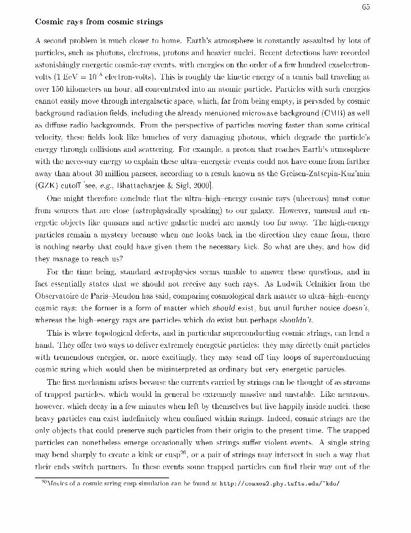
65

Cosmic rays from cosmic strings

A second problem is much closer to home. Earth's atmosphere is constantly assaulted by lots of

particles, such as photons, electrons, protons and heavier nuclei. Recent detections have recorded

astonishingly energetic cosmic-ray events, with energies on the order of a few hundred exaelectron-

volts (1 EeV = 1018 electron-volts). This is roughly the kinetic energy of a tennis ball traveling at

over 150 kilometers an hour, all concentrated into an atomic particle. Particles with such energies

cannot easily move through intergalactic space, which, far from being empty, is pervaded by cosmic

background radiation elds, including the already mentioned microwave background (CMB) as well

as diuse radio backgrounds. From the perspective of particles moving faster than some critical

velocity, these elds look like bunches of very damaging photons, which degrade the particle's

energy through collisions and scattering. For example, a proton that reaches Earth's atmosphere

with the necessary energy to explain these ultraenergetic events could not have come from farther

away than about 30 million parsecs, according to a result known as the Greisen-Zatsepin-Kuz'min

(GZK) cuto [see, e.g., Bhattacharjee & Sigl, 2000].

One might therefore conclude that the ultrahighenergy cosmic rays (uhecrons) must come

from sources that are close (astrophysically speaking) to our galaxy. However, unusual and en-

ergetic objects like quasars and active galactic nuclei are mostly too far away. The high-energy

particles remain a mystery because when one looks back in the direction they came from, there

is nothing nearby that could have given them the necessary kick. So what are they, and how did

they manage to reach us?

For the time being, standard astrophysics seems unable to answer these questions, and in

fact essentially states that we should not receive any such rays. As Ludwik Celnikier from the

Observatoire de ParisMeudon has said, comparing cosmological dark matter to ultrahighenergy

cosmic rays: the former is a form of matter which should exist, but until further notice doesn't,

whereas the highenergy rays are particles which do exist but perhaps shouldn't.

This is where topological defects, and in particular superconducting cosmic strings, can lend a

hand. They oer two ways to deliver extremely energetic particles: they may directly emit particles

with tremendous energies, or, more excitingly, they may send o tiny loops of superconducting

cosmic string which would then be misinterpreted as ordinary but very energetic particles.

The rst mechanism arises because the currents carried by strings can be thought of as streams

of trapped particles, which would in general be extremely massive and unstable. Like neutrons,

however, which decay in a few minutes when left by themselves but live happily inside nuclei, these

heavy particles can exist indenitely when conned within strings. Indeed, cosmic strings are the

only objects that could preserve such particles from their origin to the present time. The trapped

particles can nonetheless emerge occasionally when strings suer violent events. A single string

may bend sharply to create a kink or cusp20, or a pair of strings may intersect in such a way that

their ends switch partners. In these events some trapped particles can nd their way out of the

20Movies of a cosmic string cusp simulation can be found at http://cosmos2.phy.tufts.edu/~kdo/

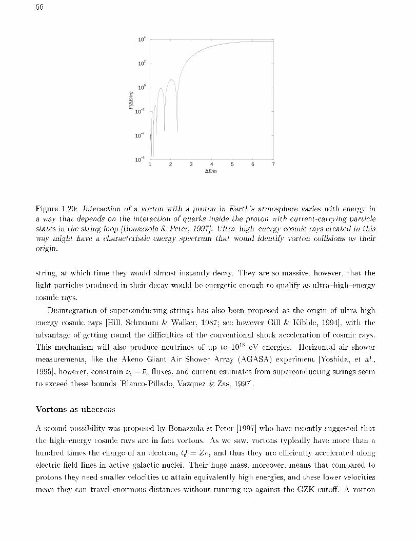
66

1 2 3 4 5 6 7∆E/m

10−6

10−4

10−2

100

102

104

F(∆

E/m

)

Figure 1.20: Interaction of a vorton with a proton in Earth's atmosphere varies with energy ina way that depends on the interaction of quarks inside the proton with current-carrying particlestates in the string loop [Bonazzola & Peter, 1997]. Ultrahighenergy cosmic rays created in thisway might have a characteristic energy spectrum that would identify vorton collisions as theirorigin.

string, at which time they would almost instantly decay. They are so massive, however, that the

light particles produced in their decay would be energetic enough to qualify as ultrahighenergy

cosmic rays.

Disintegration of superconducting strings has also been proposed as the origin of ultra high

energy cosmic rays [Hill, Schramm & Walker, 1987; see however Gill & Kibble, 1994], with the

advantage of getting round the diÆculties of the conventional shock acceleration of cosmic rays.

This mechanism will also produce neutrinos of up to 1018 eV energies. Horizontal air shower

measurements, like the Akeno Giant Air Shower Array (AGASA) experiment [Yoshida, et al.,

1995], however, constrain e + e uxes, and current estimates from superconducting strings seem

to exceed these bounds [Blanco-Pillado, Vazquez & Zas, 1997].

Vortons as uhecrons

A second possibility was proposed by Bonazzola & Peter [1997] who have recently suggested that

the highenergy cosmic rays are in fact vortons. As we saw, vortons typically have more than a

hundred times the charge of an electron, Q = Ze, and thus they are eÆciently accelerated along

electric eld lines in active galactic nuclei. Their huge mass, moreover, means that compared to

protons they need smaller velocities to attain equivalently high energies, and these lower velocities

mean they can travel enormous distances without running up against the GZK cuto. A vorton

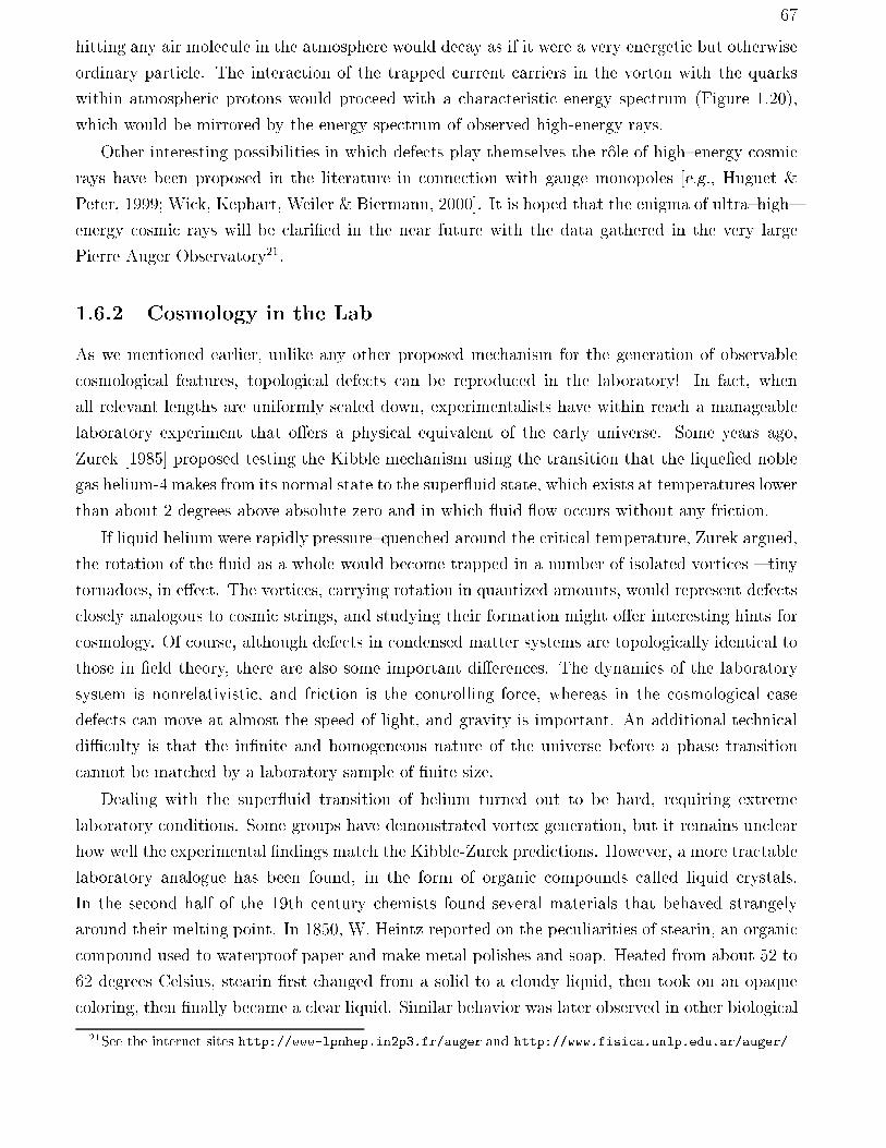
67

hitting any air molecule in the atmosphere would decay as if it were a very energetic but otherwise

ordinary particle. The interaction of the trapped current carriers in the vorton with the quarks

within atmospheric protons would proceed with a characteristic energy spectrum (Figure 1.20),

which would be mirrored by the energy spectrum of observed high-energy rays.

Other interesting possibilities in which defects play themselves the role of highenergy cosmic

rays have been proposed in the literature in connection with gauge monopoles [e.g., Huguet &

Peter, 1999; Wick, Kephart, Weiler & Biermann, 2000]. It is hoped that the enigma of ultrahigh

energy cosmic rays will be claried in the near future with the data gathered in the very large

Pierre Auger Observatory21.

1.6.2 Cosmology in the Lab

As we mentioned earlier, unlike any other proposed mechanism for the generation of observable

cosmological features, topological defects can be reproduced in the laboratory! In fact, when

all relevant lengths are uniformly scaled down, experimentalists have within reach a manageable

laboratory experiment that oers a physical equivalent of the early universe. Some years ago,

Zurek [1985] proposed testing the Kibble mechanism using the transition that the liqueed noble

gas helium-4 makes from its normal state to the super uid state, which exists at temperatures lower

than about 2 degrees above absolute zero and in which uid ow occurs without any friction.

If liquid helium were rapidly pressurequenched around the critical temperature, Zurek argued,

the rotation of the uid as a whole would become trapped in a number of isolated vortices tiny

tornadoes, in eect. The vortices, carrying rotation in quantized amounts, would represent defects

closely analogous to cosmic strings, and studying their formation might oer interesting hints for

cosmology. Of course, although defects in condensed matter systems are topologically identical to

those in eld theory, there are also some important dierences. The dynamics of the laboratory

system is nonrelativistic, and friction is the controlling force, whereas in the cosmological case

defects can move at almost the speed of light, and gravity is important. An additional technical

diÆculty is that the innite and homogeneous nature of the universe before a phase transition

cannot be matched by a laboratory sample of nite size.

Dealing with the super uid transition of helium turned out to be hard, requiring extreme

laboratory conditions. Some groups have demonstrated vortex generation, but it remains unclear

how well the experimental ndings match the Kibble-Zurek predictions. However, a more tractable

laboratory analogue has been found, in the form of organic compounds called liquid crystals.

In the second half of the 19th century chemists found several materials that behaved strangely

around their melting point. In 1850, W. Heintz reported on the peculiarities of stearin, an organic

compound used to waterproof paper and make metal polishes and soap. Heated from about 52 to

62 degrees Celsius, stearin rst changed from a solid to a cloudy liquid, then took on an opaque

coloring, then nally became a clear liquid. Similar behavior was later observed in other biological

21See the internet sites http://www-lpnhep.in2p3.fr/auger and http://www.fisica.unlp.edu.ar/auger/

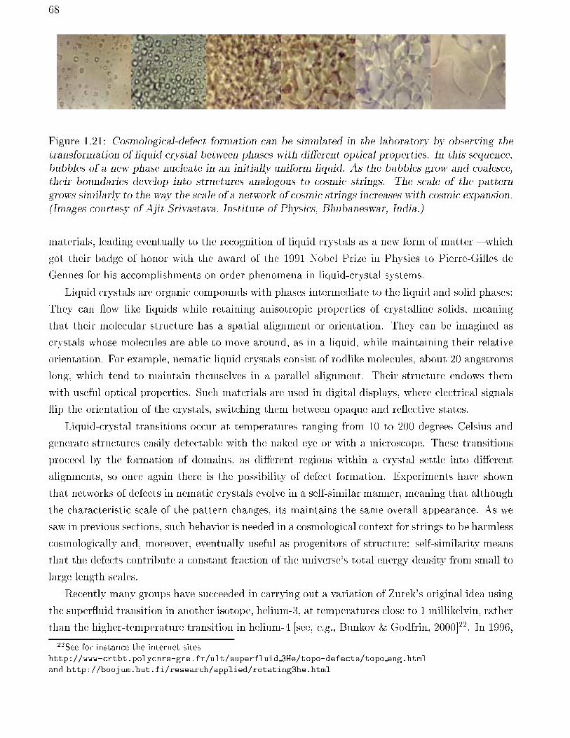
68

Figure 1.21: Cosmological-defect formation can be simulated in the laboratory by observing thetransformation of liquid crystal between phases with dierent optical properties. In this sequence,bubbles of a new phase nucleate in an initially uniform liquid. As the bubbles grow and coalesce,their boundaries develop into structures analogous to cosmic strings. The scale of the patterngrows similarly to the way the scale of a network of cosmic strings increases with cosmic expansion.(Images courtesy of Ajit Srivastava, Institute of Physics, Bhubaneswar, India.)

materials, leading eventually to the recognition of liquid crystals as a new form of matter which

got their badge of honor with the award of the 1991 Nobel Prize in Physics to Pierre-Gilles de

Gennes for his accomplishments on order phenomena in liquid-crystal systems.

Liquid crystals are organic compounds with phases intermediate to the liquid and solid phases:

They can ow like liquids while retaining anisotropic properties of crystalline solids, meaning

that their molecular structure has a spatial alignment or orientation. They can be imagined as

crystals whose molecules are able to move around, as in a liquid, while maintaining their relative

orientation. For example, nematic liquid crystals consist of rodlike molecules, about 20 angstroms

long, which tend to maintain themselves in a parallel alignment. Their structure endows them

with useful optical properties. Such materials are used in digital displays, where electrical signals

ip the orientation of the crystals, switching them between opaque and re ective states.

Liquid-crystal transitions occur at temperatures ranging from 10 to 200 degrees Celsius and

generate structures easily detectable with the naked eye or with a microscope. These transitions

proceed by the formation of domains, as dierent regions within a crystal settle into dierent

alignments, so once again there is the possibility of defect formation. Experiments have shown

that networks of defects in nematic crystals evolve in a self-similar manner, meaning that although

the characteristic scale of the pattern changes, its maintains the same overall appearance. As we

saw in previous sections, such behavior is needed in a cosmological context for strings to be harmless

cosmologically and, moreover, eventually useful as progenitors of structure: self-similarity means

that the defects contribute a constant fraction of the universe's total energy density from small to

large length scales.

Recently many groups have succeeded in carrying out a variation of Zurek's original idea using

the super uid transition in another isotope, helium-3, at temperatures close to 1 millikelvin, rather

than the higher-temperature transition in helium-4 [see, e.g., Bunkov & Godfrin, 2000]22. In 1996,

22See for instance the internet siteshttp://www-crtbt.polycnrs-gre.fr/ult/superfluid 3He/topo-defects/topo eng.html

and http://boojum.hut.fi/research/applied/rotating3he.html

69

Frequency (Hz)101 105 10

COBE

LIGO I

LIGO II/VIRGO

LISA

Pulsartiming

0.9K gravitonblackbodyradiation

Extended inflation transition

First-orderEW-scaletransition

Local strings

Global strings

Slow-roll inflation - upper bound

Chaotic inflation

Power law inflation10

10

10

10

10

10

-16

-14

-12

-10

-8

-6

10

10

10

10

10

10

-16

-14

-12

-10

-8

-6

g2

10-15 10 10-10 -5

Spec

tral

den

sity

(Ω

h ) matter

radiation

Figure 1.22: A summary of the spectral density versus frequency for various potential sourcesof a stochastic gravitational wave background. Included in this busy plot are the amplitudes ofGW from dierent types of in ationary scenarios, from a rstorder electroweak phase transition,and from both gauge and global cosmic strings, also including the primordial 0.9 K blackbodyspectrum of gravitons. [Battye & Shellard, 1996].

Ruutu and collaborators in Helsinki succeeded in heating up a volume of super uid helium-3

with thermal neutrons to just above the transition temperature, then cooling it back through the

super uid transition. They observed copious production of quantized vortices. The precision in

these experiments is such that the number of vortex lines can be monitored, allowing quantitative

testing of defect-formation theories. Laboratory tests using both liquid crystals and helium have

provided a kind of experimental conrmation of cosmological topological defect theory, increasing

the credibility of these ideas.

1.6.3 Gravitational waves from strings

Next generation of gravitational waves instruments yield a good prospect of detecting a stochastic

GW background generated in the very early universe. This opens up a brand new window, in

some sense comparable to the advent of radioastronomy to complement the existing (and as we

know, limited) opticalastronomy, many years ago now. In fact, if one had to limit oneself to those

events accessible through electromagnetic radiation alone, many of the most interesting of these

events would remain outside our reach. The CMB provides a snapshot of the universe at about

400,000 years, just as the universe became transparent to electromagnetic radiation. But what

about those processes that happened before the photon decoupling `surface'?

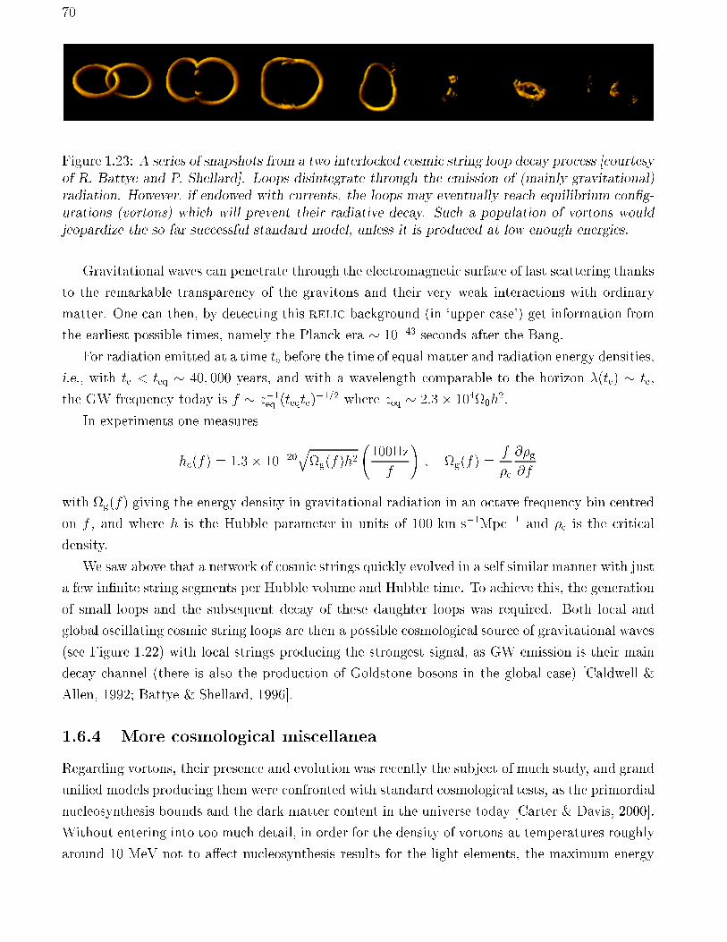
70

Figure 1.23: A series of snapshots from a two interlocked cosmic string loop decay process [courtesyof R. Battye and P. Shellard]. Loops disintegrate through the emission of (mainly gravitational)radiation. However, if endowed with currents, the loops may eventually reach equilibrium cong-urations (vortons) which will prevent their radiative decay. Such a population of vortons wouldjeopardize the so far successful standard model, unless it is produced at low enough energies.

Gravitational waves can penetrate through the electromagnetic surface of last scattering thanks

to the remarkable transparency of the gravitons and their very weak interactions with ordinary

matter. One can then, by detecting this relic background (in `upper case') get information from

the earliest possible times, namely the Planck era 1043 seconds after the Bang.

For radiation emitted at a time te before the time of equal matter and radiation energy densities,

i.e., with te < teq 40; 000 years, and with a wavelength comparable to the horizon (te) te,

the GW frequency today is f z1eq (teqte)1=2 where zeq 2:3 1040h

2.

In experiments one measures

hc(f) = 1:3 1020qg(f)h2

100Hz

f

!; g(f) =

f

c

@g@f

with g(f) giving the energy density in gravitational radiation in an octave frequency bin centred

on f , and where h is the Hubble parameter in units of 100 km s1Mpc1 and c is the critical

density.

We saw above that a network of cosmic strings quickly evolved in a self similar manner with just

a few innite string segments per Hubble volume and Hubble time. To achieve this, the generation

of small loops and the subsequent decay of these daughter loops was required. Both local and

global oscillating cosmic string loops are then a possible cosmological source of gravitational waves

(see Figure 1.22) with local strings producing the strongest signal, as GW emission is their main

decay channel (there is also the production of Goldstone bosons in the global case) [Caldwell &

Allen, 1992; Battye & Shellard, 1996].

1.6.4 More cosmological miscellanea

Regarding vortons, their presence and evolution was recently the subject of much study, and grand

unied models producing them were confronted with standard cosmological tests, as the primordial

nucleosynthesis bounds and the dark matter content in the universe today [Carter & Davis, 2000].

Without entering into too much detail, in order for the density of vortons at temperatures roughly

around 10 MeV not to aect nucleosynthesis results for the light elements, the maximum energy

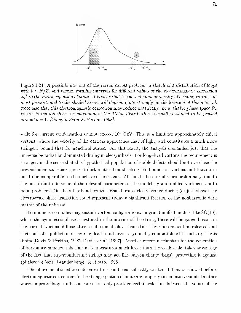
71

::::::::::::::::::::::::::::::::::::::::::

::::::::::::::::::::::::::::::::::::::::::::::::::::::::::::::::::::::::::::::::::::::::::::::::::::::::::::::::::::::::::::::::::::::::::::

b

λq 2 λq 2 λq 2 λq 2+2 +2

AB

dN/db

(A) (A) (B) (B)

Figure 1.24: A possible way out of the vorton excess problem: a sketch of a distribution of loopswith b ' N=Z, and vortonforming intervals for dierent values of the electromagnetic correctionq2 to the vorton equation of state. It is clear that the actual number density of ensuing vortons, atmost proportional to the shaded areas, will depend quite strongly on the location of this interval.Note also that this electromagnetic correction may reduce drastically the available phase space forvorton formation since the maximum of the dN=db distribution is usually assumed to be peakedaround b = 1. [Gangui, Peter & Boehm, 1998].

scale for current condensation cannot exceed 105 GeV. This is a limit for approximately chiral

vortons, where the velocity of the carriers approaches that of light, and constitutes a much more

stringent bound that for nonchiral states. For this result, the analysis demanded just that the

universe be radiation dominated during nucleosynthesis. For longlived vortons the requirement is

stronger, in the sense that this hypothetical population of stable defects should not overclose the

present universe. Hence, present dark matter bounds also yield bounds on vortons and these turn

out to be comparable to the nucleosynthesis ones. Although these results are preliminary, due to

the uncertainties in some of the relevant parameters of the models, grand unied vortons seem to

be in problems. On the other hand, vortons issued from defects formed during (or just above) the

electroweak phase transition could represent today a signicant fraction of the nonbaryonic dark

matter of the universe.

Fermionic zero modes may sustain vorton congurations. In grand unied models, like SO(10),

where the symmetric phase is restored in the interior of the string, there will be gauge bosons in

the core. If vortons diuse after a subsequent phase transition these bosons will be released and

their outofequilibrium decay may lead to a baryon asymmetry compatible with nucleosynthesis

limits [Davis & Perkins, 1997; Davis, et al., 1997]. Another recent mechanism for the generation

of baryon asymmetry, this time at temperatures much lower than the weak scale, takes advantage

of the fact that superconducting strings may act like baryon charge `bags', protecting it against

sphaleron eects [Brandenberger & Riotto, 1998].

The above mentioned bounds on vortons can be considerably weakened if, as we showed before,

electromagnetic corrections to the string equation of state are properly taken into account. In other

words, a protoloop can become a vorton only provided certain relations between the values of the

72

conserved parameters characterizing the vorton hold. We have seen that these relations (embodied

in the relevant master function of the string) change whenever electromagnetic self couplings are

considered. A given distribution of vortons will be characterized by the ratio of the conserved

numbers b ' N=Z. As it turns out, increasing the electromagnetic correction is equivalent to

reducing the available phase space for vorton formation, as b of order unity is the most natural

value [see, e.g., Brandenberger, Carter, Davis & Trodden, 1996] situation that we sketch in Figure

1.24. On this gure, we have assumed a sharply peaked dN=db distribution centered around b = 1;

with q2 = 0, the available range for vorton formation lies precisely where the distribution is

maximal, whereas for any other value, it is displaced to the right of the distribution. Assuming

a Gaussian distribution, this eect could easily lead to a reduction of a few orders of magnitude

in the resulting vorton density, the latter being proportional to the area below the distribution

curve in the allowed interval. This means that as the string loops contract and loose energy in the

process, they keep their `quantum numbers' Z and N constant, and some sets of such constants

which, had they been decoupled from electromagnetism, would have ended up to equilibrium

vorton congurations, instead decay into a bunch of Higgs particles, themselves unstable. This

may reduce the cosmological vorton excess problem if those are electromagnetically charged.

The cosmic microwave background radiation might also be used as a charged string loop detec-

tor. In fact vortons are like point masses with quantized electric charge and angular momentum.

They are peculiar for, if they are formed at the electroweak scale, their characteristic size cannot

be larger than a hundredth the classical electron radius, while their mass would be some ve orders

of magnitude heavier than the electron. They can however contain up to 1 137 times the elec-

tron charge, and hence Thomson scattering between vortons and the cosmic background radiation

at recombination would be (we are admittedly optimistic in here) just nearly at the same level

as the standard one, with important consequences for, e.g., the polarization of the relic radiation.

The signature would depend on the actual distribution of relic vortons at z 1000, an input that

is presently largely unknown. According to current estimates [e.g., Martins & Shellard, 1998b],

electroweak vortons could contribute nonnegligibly to the energy density. However, current g-

ures are still well below what is needed to get a distinguishable signal from them and thus their

CMB trace would be hidden in the `noise' of the vastly too numerous electrons.

Acknowledgments

For these lectures I've drawn freely from various sources. I thank the people who kindly provided

gures and discussions. Among them, I owe special debts to Brandon Carter, Jerome Martin,

Patrick Peter, Levon Pogosian, and Serge Winitzki for very enjoyable recent collaborations. Thanks

also to the other speakers and students for the many discussions during this very instructive study

week we spent together, and to the members of the L.O.C. for their superb job in organizing

this charming school. A.G. thanks CONICET, UBA and Fundacion Antorchas for nancial

support.

Bibliography

[1] Abrikosov, A. A. [1957], Sov. Phys. JETP 5, 1174 [Zh. Eksp. Teor. Fiz. 32, 1442 (1957)]

[2] Achucarro, A. & Vachaspati, T. [2000], Phys. Rept. 327, 347-426; Phys. Rept. 327, 427. [hep-ph/9904229]

[3] Albrecht, A., Battye, R. & Robinson, J. [1997], Phys. Rev. Lett. 79, 4736.; Phys. Rev. D59, 023508 (1998).

[4] Albrecht, A., Coulson, D., Ferreira, P. & Magueijo, J. [1995], Imperial Preprint /TP/9495/30.

[5] Alexander, S., Brandenberger, R., Easther, R. & Sornborger, A. [1999], hep-ph/9903254.

[6] Allen, B. & Shellard, E.P.S. [1990], Phys. Rev. Lett. 64, 119.

[7] Avelino, P.P. & Martins, C.J.A.P. [2000], Phys. Rev. Lett. 85, 1370.

[8] Avelino, P.P., Shellard, E.P.S., Wu, J.H.P. & Allen, B. [1998], Astrophys. J. 507, L101.

[9] Bartelmann, M. & Schneider, P. [2001], Phys. Rep. 340, 291.

[10] Bhattacharjee, P. & Sigl, G. [2000], Phys. Rep. 327, 109-247.

[11] Battye, R. & Weller, J. [2000], Phys. Rev. D61, 043501.

[12] Benabed, K. & Bernardeau, F. [2000], Phys. Rev. D61, 123510.

[13] Bennett, C.L., et al. [1992], Ap. J. Lett. 396, L7.

[14] Bennett, C.L., et al. [1994], Ap. J. 430, 423.

[15] Bennet, D.P. [1986], Phys. Rev. D24, 872; ibid D34, 3592 (1986).

[16] Bennett, D.P. & Bouchet, F.R. [1988], Phys. Rev. Lett. 60, 257.

[17] Bennett, D.P. & Rhie, S.H. [1990], Phys. Rev. Lett. 65, 1709.

[18] Bennett, D.P. & Rhie, S.H. [1993], Ap. J. Lett. 406, L7.

[19] Bennett, D.P., Rhie, S.H. & Weinberg, D.H. [1993], preprint.

[20] Bennett, D.P., Stebbins, A. & Bouchet, F.R. [1992], Ap. J. Lett. 399, L5.

[21] Blanco-Pillado, J., Vazquez, R. & Zas, E. [1997], Phys. Rev. Lett. 78, 3614. [astro-ph/9612010]

[22] Bonazzola, S. & P. Peter [1997], Astroparticle Physics 7, 161-172.

[23] Borrill, J., et al. [1994], Phys. Rev. D50, 2469.

[24] Bouchet, F. R., Bennett, D. P. & Stebbins, A. [1988], Nature 335, 410.

[25] Bouchet, F.R., Peter, P., Riazuelo, A. & Sakellariadou, M. [2001] preprint astro-ph/0005022.

[26] Bowick, M., Chandar, L., Schi, E. & Srivastava, A. [1994], Science 236, 943.

73

74 REFERENCES

[27] Brandenberger, R. [1993], Topological Defects and Structure Formation, EPFL lectures, Lausanne, Switzer-land.

[28] Brandenberger, R., Carter, B., Davis, A.C. & Trodden, M. [1996], Phys. Rev. D54, 6059.

[29] Brandenberger, R. & Riotto, A. [1998], [hep-ph/9801448]

[30] Bunkov, Y. & Godfrin, H. [2000], (editors) Proceedings of the NATO-ASI on topological defects and non-equilibrium dynamics of symmetry breaking phase transitions (Kluwer, Dordrecht).

[31] Carter, B. [1989] Phys. Lett. B224, 61; Phys. Lett. B228, 466.

[32] Carter, B, [1990], Phys. Rev. D41, 3869.

[33] Carter, B. [1997], Tlaxcala lecture notes, hep-th/9705172.

[34] Carter, B. [1997b], Phys. Lett. B404, 246.

[35] Carter, B. & Davis, A. [2000], Phys. Rev. D61, 123501.

[36] Carter, B. & Peter, P. [1995], Phys. Rev. D52, R1744.

[37] Carter, B., Peter, P. & Gangui, A. [1997], Phys. Rev. D55, 4647. [hep-ph/9609401];

[38] Chuang, I. [1994], private communication, 1994.

[39] Chuang, I., Durrer, R., Turok, N. & Yurke, B. [1991], Science 251, 1336.

[40] Contaldi, C., Hindmarsh, M. & Magueijo, J. [1999], Phys. Rev. Lett. 82 2034.

[41] Copeland, E. [1993], in The physical universe: The interface between cosmology, astrophysics and particle

physics, eds. Barrow, J.D., et al. (SringerVerlag).

[42] Coulson, D., Ferreira, P., Graham, P. & Turok, N. [1994], Nature 368, 27.

[43] Cowie, L. & Hu, E. [1987], Ap. J.318 L33.

[44] Davis, A. C. & Perkins, W. B. [1997], Phys. Lett. B393, 46.

[45] Davis, S.C., Davis, A. C. & Perkins, W. B. [1997], Phys. Lett. B408, 81.

[46] Davis, R.L. & Shellard, E.P.S. [1988], Phys. Lett. B207, 404.

[47] de Bernardis, P. et al. [2000], Nature 404, 995 [astro-ph/0004404]

[48] de Gennes, P. [1974], The Physics of Liquid Crystals (Clarendon Press, Oxford).

[49] de Laix, A.A. & Vachaspati, T. [1996], Phys. Rev. D54, 4780.

[50] de Zotti, G. et al.[1999], astroph/9908058.

[51] Dolan, L. & Jackiw, R. [1974], Phys. Rev. D9, 3320.

[52] Durrer, R. [1994], Fund. of Cosmic Physics 15, 209.

[53] Durrer, R. [2000], in Moriond meeting on Energy Densities in the Universe, astro-ph/0003363 .

[54] Durrer, R., Gangui, A. & Sakellariadou, M. [1996], Phys. Rev. Lett. 76, 579. [astro-ph/9507035].

[55] Durrer, R. & Zhou, Z.H. [1995], Zurich University Preprint, ZHTH19/95, astroph/9508016.

[56] Durrer, R., Howard, A. & Zhou, Z.H. [1994], Phys. Rev. D49, 681.

[57] Dvali, G., Liu, H. & Vachaspati, T. [1998], Phys. Rev. Lett. 80, 2281.

REFERENCES 75

[58] Gangui, A. [2001], Science 291, 837.

[59] Gangui, A., Lucchin, F., Matarrese, S. & Mollerach, S. [1994], Ap. J. 430, 447.

[60] Gangui, A. & Martin, J. [2000a], Mon. Not. R. Astron. Soc. 313, 323. [astro-ph/9908009]

[61] Gangui, A. & Martin, J. [2000b], Phys. Rev. D62, 103004. [astro-ph/0001361]

[62] Gangui, A. & Mollerach, S. [1996], Phys. Rev. D54, 4750-4756. [astro-ph/9601069]

[63] Gangui, A. & Peter, P. [1998], Cosmological and Astrophysical Implications of Superconducting CosmicStrings and Vortons, in Proceedings of the XXXIIIrd Rencontres de Moriond on `Fundamental Parametersin Cosmology', pages 19 - 24, Editors: J. Tran Thanh Van et al, Editions Frontieres, 1998.

[64] Gangui, A., Peter, P. & Boehm, C. [1998], Phys. Rev. D57, 2580. [hep-ph/9705204]

[65] Gangui, A., Peter, P. & Gunzig, E. [1999], Int. Journal of Theor. Physics, 38, 205-216.

[66] Gangui, A., Pogosian, L. & Winitzki, S. [2001a], New Astronomy Reviews, to appear.

[67] Gangui, A., Pogosian, L. & Winitzki, S. [2001b], Phys. Rev. D64, 043001.

[68] Gill, A. & Kibble, T. [1994], Phys. Rev. D50, 3660. [hep-ph/9403395]

[69] Goto, T. [1971], Prog. Theor. Phys. 46, 1560.

[70] Gott, R. [1985], Ap. J., 288, 422.

[71] Guth, A.H. [1981], Phys. Rev. D23, 347.

[72] Guth, A.H. & Pi, S.Y. [1985], Phys. Rev. D32, 1899.

[73] Guth, A.H. & Tye, S.H. [1980], Phys. Rev. Lett. 44, 631.

[74] Guth, A.H. & Weinberg, E. [1983], Nucl. Phys. B212, 321.

[75] Halliwell, J.J. [1989], Phys. Rev. D39, 2912.

[76] Hanany, S., et al, Astrophys. J. Lett. accepted (2000), astro-ph/0005123; Jae, A.H., et al, astro-ph/0007333.

[77] Hancock, S., Davies, R.D., Lasenby, A.N., Gutierrez de la Cruz, C.M., Watson, R.A., Rebolo, R. & Beckman,J.E. [1994], Nature 367, 333.

[78] N.W. Halverson, et al, preprint astro-ph/0104489.

[79] Hara T. Mahonen, P. & Miyoshi S. [1993], Ap. J. 414, 421.

[80] Hara T. & Miyoshi S. [1993], Ap. J. 405, 419.

[81] Harrison, R. [1970], Phys. Rev. D1, 2726.

[82] Hedman, M., Barkats, D., Gundersen, J. Staggs, S. & Winstein, B. [2001], Ap. J., 548, L111-L114 [astro-ph/0010592].

[83] Hendry, P.C., Lawson, N.S., Lee, R.A.M., McClintock, P.V.E. & Williams, C.D.H. [1994], Nature 368, 315.

[84] Higgs, P. [1964], Phys. Lett. 12, 132.

[85] Hill, C., Schramm, D. & Walker, T. [1987], Phys. Rev. D36, 1007.

[86] Hilton, P.J. [1953], Introduction to homotopy theory (Cambridge: Cambridge University Press).

[87] Hindmarsh M. [1994], Ap. J. 431, 534.

76 REFERENCES

[88] Hindmarsh, M.B. & Kibble, T.W.B. [1995], Rept. Prog. Phys. 58, 477-562 [hep-ph/9411342].

[89] Hu, W., Scott, D. & Silk, J. [1994], Phys. Rev. D49, 648.

[90] Hu, W., Spergel, D. & White, M. [1997], Phys. Rev. D55, 3288-3302.

[91] Huguet, E. & Peter, P. [2000], Astropart. Phys. 12, 277-289.

[92] Kaiser, N. & Stebbins, A. [1984], Nature 310, 391.

[93] Kamionkowski, M., Spergel, D.N. & Sugiyama, N. [1994], Ap. J. Lett. 426, L57.

[94] Kasuya, S. & Kawasaki, M, [1998], Phys. Rev. D58, 083516.

[95] Kibble, T.W.B. [1976], J. Phys. A9, 1387.

[96] Kibble, T.W.B. [1980], Phys. Rep. 67, 183.

[97] Kibble, T.W.B. [1985], Nucl. Phys. B252, 227; B261, 750 (1986).

[98] Kibble, T.W.B., Lazarides, G. & Sha, Q. [1982], Phys. Lett. B113, 237.

[99] Kirzhnits, D.A. & Linde, A.D. [1974], Sov. Phys. JETP 40, 628.

[100] Kirzhnits, D.A. & Linde, A.D. [1976], Ann. Phys. 101, 195.

[101] Kodama, H. & Sasaki, M. [1984], Prog. Theor. Phys. Suppl. 78, 1.

[102] Kofman, L.A., Linde, A.D. & Starobinskii, A.A. [1985], Phys. Lett. B157, 361.

[103] Kofman, L.A., Linde, A.D. & Starobinskii, A.A. [1994], Phys. Rev. Lett. 24, 3195.

[104] Kolb, E.W. & Turner, M.S. [1990] The Early Universe (New York: AddisonWesley).

[105] Komatsu, E. & Spergel, D. [2000], preprint astro-ph/0005036; Wang, L. & Kamionkowski, M. [2000], Phys.Rev. D61, 063504.

[106] Langacker, P. & Pi, S.Y. [1980], Phys. Rev. Lett. 45, 1.

[107] Langer, S. [1992], in Solids far from equilibrium, Godreche, C., ed. (Cambridge: Cambridge UniversityPress).

[108] Liddle, A. [1995], Phys. Rev. D51, 5347-5351.

[109] Linde, A.D. [1983b], Nucl. Phys. B216, 421.

[110] Linde, A.D. [1990], Particle Physics and In ationary Cosmology (Harwood, Chur, Switzerland).

[111] Linde, A.D. [1994], Phys. Rev. D49, 748.

[112] Linet, B. [1986], Phys. Rev. D33 1833.

[113] Luo, X. [1994], Ap. J. Lett. 427, L71.

[114] Lucchin, F. & Matarrese, S. [1985], Phys. Rev. D32, 1316.

[115] Magueijo, J. , Albrecht, A. , Ferreira, P. & Coulson, D. [1996], Phys. Rev. D54, 3727-3744.

[116] Magueijo, J. & Brandenberger, R. [2000], Iran lectures on cosmic defects, astro-ph/0002030.

[117] Magueijo, J. & Ferreira, P. [1997], Phys. Rev. D55, 3358.

[118] Martins, C.J.A.P. & Shellard, E.P.S. [1996], Phys. Rev. D54 2535.

REFERENCES 77

[119] Martins, C.J.A.P. & Shellard, E.P.S. [1998], Phys. Rev. D57, 5276. [astro-ph/9706287]

[120] Martins, C.J.A.P. & Shellard, E.P.S. [1998b], Phys. Rev. D57, 7155.

[121] Martins, C.J.A.P. & Shellard, E.P.S. [2000], hep-ph/0003298

[122] Mermin, M. [1979] , Rev. Mod. Phys. 51, 591.

[123] Nambu, Y. [1970], in Proc. Int. Conf. on Symmetries and Quark Models, ed. Chand, R. (New York: Gordonand Breach).

[124] Notzold, D. [1991], Phys. Rev. D43, R961.

[125] Pen, U.-L., Seljak, U. & Turok, N. [1997], Phys. Rev. Lett. 79, 1611-1614.

[126] Pen, U.L., Spergel, D.N. & Turok, N. [1994], Phys. Rev. D49, 692.

[127] Penzias, A.A. & Wilson, R.W. [1965], Ap. J. 142, 419.

[128] Peter, P. [1992], Phys. Rev. D46, 3335.

[129] Peter, P. [1993], Phys. Rev. D47, 3169.

[130] Pogosian, L. [2000], astro-ph/0009307.

[131] Pogosian, L. & Vachaspati, T. [1999], Phys. Rev. D60, 083504.

[132] Pogosian, L. & Vachaspati, T. [2000], Phys. Rev. D62, 105005.

[133] Preskill, J. [1979], Phys. Rev. Lett. 43, 1365.

[134] Rajaraman, R. [1982], Solitons and instantons (Amsterdam: NorthHolland).

[135] Sachs, R. & Wolfe, A. [1967], Ap. J. 147, 73.

[136] Scaramella, R. & Vittorio, N. [1991], Ap. J. 375, 439.

[137] Scaramella, R. & Vittorio, N. [1993], M.N.R.A.S. 263, L17.

[138] Scott, D., Srednicki, M. & White, M. [1994], Ap. J. Lett. 421, L5.

[139] Seljak, U., Pen, U.-L. & Turok, N. [1997], Phys.Rev.Lett. 79 1615-1618.

[140] Seljak, U. & Zaldarriaga, M. [1996], Astrophys. J. 469, 437.

[141] Seljak, U. & Zaldarriaga, M. [1997], Phys. Rev. Lett. 78, 2054.

[142] Silk, J. [1968], Ap. J. 151, 459.

[143] Silk, J. & Vilenkin, A. [1984], Phys. Rev. Lett. 53, 1700.

[144] Smith, G. & Vilenkin, A. [1987], Phys. Rev. D36, 990.

[145] Smoot, G.F., et al. [1992], Ap. J. Lett. 396, L1.

[146] Srednicki, M. [1993], Ap. J. Lett. 416, L1.

[147] Stebbins, A. [1988], Ap. J. 327, 584.

[148] Stebbins, A., et al. [1987], Ap. J. 322, 1.

[149] Steenrod, N. [1951], Topology of Fibre Bundles (Princeton: Princeton University Press).

78 REFERENCES

[150] Tinkham, M. [1995], Introduction To Superconductivity, 2nd edition, McGraw-Hill Higher Education, NewYork.

[151] Tkachev, I., Khlebnikov, S., Kofman, L. & Linde, A. [1998], Phys.Lett. B440, 262-268.

[152] Turok, N. [1989], Phys. Rev. Lett. 63, 2625.

[153] Turok, N. [1996], Phys. Rev. Lett. 77, 4138-4141; Phys. Rev. D54, 3686-3689

[154] Turok, N., Pen, U.-L. & Seljak, U. [1998], Phys. Rev. D58, 023506.

[155] Turok, N. & Spergel, D.N. [1990], Phys. Rev. Lett. 64, 2736.

[156] Turok, N. & Zadrozny, J. [1990], Phys. Rev. Lett. 65, 2331.

[157] Vachaspati, T. [2001], ICTP summer school lectures, hep-ph/0101270.

[158] Vachaspati, T. & Vilenkin, A. [1991], Phys. Rev. Lett. 67, 1057.

[159] Veeraraghavan, S. & Stebbins, A. [1990], Ap. J. 365, 37.

[160] Vilenkin, A. [1981], Phys. Rev. D23, 852.

[161] Vilenkin, A. [1983], Phys. Rev. D27, 2848.

[162] Vilenkin, A. [1985], Phys. Rep. 121, 263.

[163] Vilenkin, A [1990], Phys. Rev. D41, 3038.

[164] Vilenkin, A. & Shellard, E.P.S. [2000], Cosmic Strings and other Topological Defects, 2nd edition, (Cam-bridge: Cambridge University Press).

[165] Vollick, D.N. [1992], Phys. Rev. D45, 1884.

[166] Walker, P.N., et al. [1991], Ap. J. 376, 51.

[167] Weinberg, S. [1972], Gravitation and Cosmology (Wiley, New York).

[168] Weinberg, S. [1974], Phys. Rev. D9, 3357.

[169] Weinberg, S., [2000], astro-ph/0006276

[170] White, M., Scott, D. & Silk, J. [1994], Ann. Rev. Astron. and Astrophys. 32, 319.

[171] Wick, S., Kephart, T., Weiler, T. & Biermann, P. [2000], Astropart. Phys. submitted. [astro-ph/0001233]

[172] Witten, E. [1985], Nucl. Phys.B249, 557.

[173] Wu, J.-H.P. et al, preprint astro-ph/9812156.

[174] Yoshida, S. et al.[1995], Astropart. Phys. 3, 105.

[175] Yurke, B. [1994], Physics World, July issue, page 28.

[176] Zaldarriaga, M. & Seljak, U. [1998], Phys. Rev. D58, 023003.

[177] Zel'dovich, Ya.B. [1970], Astron. Astrophys. 5, 84.

[178] Zel'dovich, Ya.B. & Sunyaev, R.A. [1969], Astrophys. Space Sci. 4, 301.

[179] Zurek, W.H. [1982], Phys. Rev. D26, 1862.

[180] Zurek, W.H. [1985], Nature 317, 505.