Kinetics Models of Granular and Active Matter: Hydrodynamics and Fluctuations Alessandro Manacorda Universit` a degli studi di Roma Sapienza January 26, 2015 Alessandro Manacorda Kinetics Models of Granular and Active Matter: Hydrodynamics
Transcript
Kinetics Models of Granular and Active Matter:
Hydrodynamics and Fluctuations
Alessandro Manacorda
Universita degli studi di Roma Sapienza
January 26, 2015
Alessandro Manacorda Kinetics Models of Granular and Active Matter: Hydrodynamics
Non-equilibrium Physics
A physical system is out of equilibrium when its macroscopicdynamics is not invariant under time inversion.
Alessandro Manacorda Kinetics Models of Granular and Active Matter: Hydrodynamics
Cooling Regimes
Homogeneity ⇒ u(x , t) = ∂x = 0⇓
Homogeneous cooling state:THCS(t) = T0e
−νt (Haff 1983)
Rescaled fields:u = u/
√THCS , T = T/THCS
→ stationary cooling state
Linear analysis:
{
∂t u(k , t) =(
ν/2− k2)
u(k , t)
∂tT (k , t) = −k2T (k , t)
⇒ homogeneous cooling stable forν < νc = 8π2
1e-05
0.0001
0.001
0.01
0.1
1
0 0.2 0.4 0.6 0.8 1
T(t
)
t
L = 1000ν = 10ν = 20ν = 30ν = 40
e-10 t
e-20 t
e-30 t
e-40 t
0.04
0.06
0.08
0.1
0.12
0.14
0.16
0.18
0 0.02 0.04 0.06 0.08 0.1 0.12u m
ax /
T1/
2 HC
S (
t)
t
A = 0.1, L = 1000ν = 68ν = 78ν = 79ν = 98
umax (t,68)umax (t,78)umax (t,79)umax (t,88)
Alessandro Manacorda Kinetics Models of Granular and Active Matter: Hydrodynamics
Nonhomogeneity
No symmetry for space translations ⇒ Nonhomogeneous regimeFirst mode → exact solution
u(x , 0) = u0 sin(2πx), T (x , 0) ≡ T0
⇓{
u(x , t) = u0 sin(2πx)e−νc t/2
T (x , t) = T0e−νt +
νcu202 e−νc t
[
1−e−(ν−νc )t
ν−νc+ cos(4πx)1−e−(ν+νc )t
ν+νc
]
.
(3)
-0.4
-0.3
-0.2
-0.1
0
0.1
0.2
0.3
0.4
0 0.1 0.2 0.3 0.4 0.5 0.6 0.7 0.8 0.9 1
u(x,
t)
x
A = 1, ν = 68, L = 1000
t = 2/ν 0.24
0.25
0.26
0.27
0.28
0.29
0.3
0 0.1 0.2 0.3 0.4 0.5 0.6 0.7 0.8 0.9 1
T(x
,t)
x
A = 1, ν = 68, L = 1000
t = 2/ν
Alessandro Manacorda Kinetics Models of Granular and Active Matter: Hydrodynamics
Correlations and Failure of LE
Numerical simulations ⇒ LE good approximation withdiscrepancies
Momentum conservation ⇒ non-zero correlationsC (x , t) = 〈v(0, t)v(x , t)〉Closed set of equations for correlations without LE ⇒diffusion equation with PB and symmetric profile
∂t C (x , t) = 2∂2x C (x , t)+νC (x , t)
Alessandro Manacorda Kinetics Models of Granular and Active Matter: Hydrodynamics
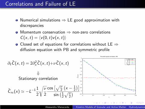
Correlations and Failure of LE
Numerical simulations ⇒ LE good approximation withdiscrepancies
Momentum conservation ⇒ non-zero correlationsC (x , t) = 〈v(0, t)v(x , t)〉Closed set of equations for correlations without LE ⇒diffusion equation with PB and symmetric profile
∂t C (x , t) = 2∂2x C (x , t)+νC (x , t)
⇓Stationary correlation
C∞(x) ≃ −L−1 1
2
√
ν
2
cos[√
ν2
(
x − 12
)]
sin(
12
√
ν2
)
-3.5
-3
-2.5
-2
-1.5
-1
-0.5
0
0.5
1
1.5
2
0 0.1 0.2 0.3 0.4 0.5
D~ (
x,t)
x
Rescaled spatial correlation, MM
L=250, ν=40νt = 0νt = 5
νt = 10D~
th(x)
Alessandro Manacorda Kinetics Models of Granular and Active Matter: Hydrodynamics
Alessandro Manacorda Kinetics Models of Granular and Active Matter: Hydrodynamics
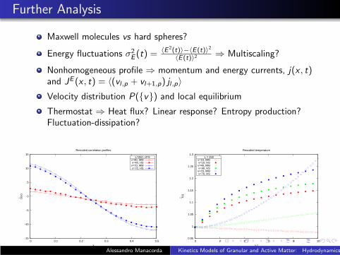
Further Analysis
Maxwell molecules vs hard spheres?
Energy fluctuations σ2E (t) =
〈E 2(t)〉−〈E(t)〉2
〈E(t)〉2 ⇒ Multiscaling?
Nonhomogeneous profile ⇒ momentum and energy currents, j(x , t)and JE (x , t) = 〈(vl,p + vl+1,p) jl,p〉Velocity distribution P({v}) and local equilibrium
Thermostat ⇒ Heat flux? Linear response? Entropy production?Fluctuation-dissipation?
-15
-10
-5
0
5
10
15
0 0.1 0.2 0.3 0.4 0.5
D~(x
)
x
Rescaled correlation profiles
L=250, νt=9ν=40, MMν=40, HSν=70, MMν=70, HS
0.95
1
1.05
1.1
1.15
1.2
1.25
1.3
0 2 4 6 8 10
T~(t
)
ν t
Rescaled temperature
L = 250ν=10, MMν=10, HSν=40, MMν=40, HSν=70, MMν=70, HS
Alessandro Manacorda Kinetics Models of Granular and Active Matter: Hydrodynamics
Perspectives
Molecular vs lattice models
Active matter have inertia ⇒ theoretical models ofself-propelled particles with inertia
General laws for fluctuations, transport coefficients, FDTbeyond phenomenological approach
Comparison with experiments and patterns for furtherinvestigations
Alessandro Manacorda Kinetics Models of Granular and Active Matter: Hydrodynamics