Alexander N. Bogin William M. Doerner William D. Larson ... · Missing the Mark: House Price Index...

Missing the Mark:House Price Index Accuracy and Mortgage Credit Modeling

Alexander N. BoginWilliam M. DoernerWilliam D. Larson

September 2016

Working Paper 16-04

FEDERAL HOUSING FINANCE AGENCYDivision of Housing Mission & GoalsOffice of Policy Analysis & Research

400 7th Street SWWashington, DC 20024, USA

Please address correspondences to William Doerner ([email protected]). Many thanksto Andy Leventis, Scott Smith, and Fred Graham, who provided helpful questions, comments,and discussion. We also thank discussants and participants from the George WashingtonUniversity’s University Seminar on Forecasting, the American Real Estate Society annualmeetings, and the AREUEA national conference. No outside funding was received for thisresearch.

Federal Housing Finance Agency (FHFA) Staff Working Papers are preliminary productscirculated to stimulate discussion and critical comment. The analysis and conclusions arethose of the authors and do not necessarily represent the views of the Federal HousingFinance Agency or the United States.

Missing the Mark: House Price Index Accuracy and Mortgage Credit ModelingAlexander N. Bogin, William M. Doerner, and William D. Larson

FHFA Staff Working Paper 16-04September 2016

Abstract

We make two contributions to the study of house price index and mortgage credit mod-eling accuracy. First, we assess the predictive power of house price indices calculatedat different levels of geographic aggregation. Lower levels of aggregation offer superiorfit when appreciation rates vary substantially across submarkets and the indices arebased on a sufficient number of transactions. Second, we estimate a competing op-tions credit model using 15 years of mortgage performance data in the United States.Model accuracy is highest when using indices at a city or lower level of aggregation toconstruct current loan-to-value ratios. Fit is weaker when using state or national priceindices. Overall, this research highlights the benefits of using more localized houseprice indices when predicting property values and mortgage performance.

Keywords: house prices · loan-to-value · mortgage performance · credit model

JEL Classification: C55 · G22 · R30 · R51

Alexander N. Bogin William M. DoernerFederal Housing Finance AgencyOffice of Policy Analysis & Research

400 7th Street SWWashington, DC 20024, [email protected]

Federal Housing Finance AgencyOffice of Policy Analysis & Research


William D. LarsonFederal Housing Finance AgencyOffice of Policy Analysis & Research


mailto:[email protected]



FHFA Working Paper 16-04

1. IntroductionRealtors have long heralded the claim that the residential housing market is driven by “lo-

cation, location, location.” Nonetheless, a variety of limitations have prevented researchers

from broadly testing the assertion that appreciation rates are dependent on a house’s par-

ticular site within a city. In finance, a better understanding of local house price dynamics

could lead to a more accurate valuation of mortgage collateral and improved estimates of

the credit risk associated with mortgage securities.1 We attempt to determine the extent to

which house price indices of different levels of granularity affect pricing accuracy, and the

consequences of using different price indices on efforts to model mortgage prepayments and

defaults.

A portfolio of mortgages can be a complex financial product to price. The value of the

underlying collateral is likely to change as a result of both longitudinal and cross-sectional

variation in house price appreciation rates. Urban real estate theory suggests that, even

within the same city, housing can appreciate at different rates (see classic studies by Bailey

et al., 1963; Alonso, 1964; Mills, 1967; Muth, 1969) for predictable reasons. But, up until now,

such within-city cross-sectional variation has been difficult to measure reliably, stymieing

research on the portfolio effects and credit risk implications of highly localized variation of

house price appreciation.

We make two main contributions to the study of house price valuation and mortgage credit

modeling. First, we assess the accuracy of house price indices (HPIs) calculated at different

levels of geographic aggregation from a database of nearly 100 million observations. The in-

dices allow us to predict sales values for a hold-out sample of individual properties and judge

accuracy based upon subsequent market transactions. In general, differences in predictive

accuracy occur when house price appreciation rates across sub-aggregates are different, and

the increased signal from a more granular index is not counterbalanced by increased vari-

ance. Aggregate HPIs are better predictors in rural areas or small cities, and during periods

of stable appreciation. Disaggregated indices produce more accurate estimates within large

cities, especially during booms and busts in housing markets when substantial submarket

appreciation differentials exist. Overall, we find the ideal level of house price index aggre-

1We are not the only ones to suggest that granular information could be advantageous in mortgagemarkets. Recently, Stroebel (2016) studies how knowing a builder’s construction quality allows certainlenders to offer lower rates and incur less severe losses through superior loan modeling.

1 A. Bogin, W. Doerner, & W. Larson — Missing the Mark


gation in large cities is at the 5-digit ZIP code level. In small cities, a city-level index is

sufficient. We also find that a linear combination of indices at a variety of different levels of

aggregation may offer superior fit.

Second, we use the HPIs to estimate mortgage performance across the United States for the

last 15 years. A primary risk factor affecting the incidence of prepayment and default is

a mortgage’s loan-to-value (LTV) ratio. In each period post-origination, the current LTV

(CLTV) ratio is recalculated to account for principal payments and the marked-to-market

value of the housing asset. Throughout the life of the loan, the CLTV is key to estimating

a borrower’s likelihood to prepay or default. To understand the full effect of potential

geographic aggregation bias, we begin by estimating a credit model where CLTV has been

constructed using a national index. Next, we recalculate CLTV ratios with increasingly

granular indices and show that using more localized HPIs generally improves model fit,

particularly in central areas of larger cities. We also uncover some interesting cases in which

increased granularity has some beneficial model impact at an individual asset level (e.g., to

better identify underwater borrowers for modifications, refinancing, or workout options) as

well as for portfolio analysis (e.g., to reduce model error in loss estimation).

The paper is structured as follows. Section 2 introduces a suite of HPIs constructed at

different levels of geography and analyzes their predictive accuracy. We run several types of

tests to investigate when and where an HPI is likely to “miss the mark.” Section 3 utilizes

the same indices to evaluate the effect of geographic aggregation bias on mortgage credit

modeling. Section 4 offers concluding thoughts.

2. Assessing House Price Index AccuracyHouse price indices can be useful for establishing an estimate of market values for individual

properties—the collateral for loans in mortgage-backed securities. The suitability of an index

depends on its predictive accuracy and the extent of its estimation error. Aggregation bias

can occur when house prices appreciate at different rates in different submarkets, and an

index constructed over several such submarkets masks those differences. Mitigating aggre-

gation bias therefore requires estimating price indices at a more local level. Estimation error

is a function of the variance of an estimator, which is affected primarily in this context by

the number of transactions over which the index is estimated. The tension in the selection of

a house price index is therefore a tradeoff between reduced aggregation bias and higher es-



timation error as index granularity increases. In this section, we investigate the appropriate

HPI aggregation level to minimize these two separate sources of error.

To foreshadow, we find that an HPI’s accuracy fluctuates over time. It tends to became

less precise as housing prices become more volatile (i.e., when prices are quickly falling or

rising). We also find that accuracy improves as we move from a national index to increasingly

disaggregated indices, although the incremental benefit from disaggregation decreases.2 As

we move to more and more local geographies, increased precision is overwhelmed by increased

estimator variance. Indices using a ZIP code level of aggregation generally minimize the

aggregate error from these competing sources, but less granular indices can perform just as

well in certain contexts. For instance, in small cities or in periods when the housing market

is growing, a city-level index will do at least as well. Next, we describe the construction of

our house prices indices, evaluation methods, and results.

2.1. House Price Measurement

We use a repeat-sales methodology to construct house price indices. A standard approach

was introduced by Bailey, Muth, and Nourse (1963) and updated by Case and Shiller (1987).

The method is attractive because of its limited data requirements (only requiring a price,

transaction date, and location) and a straightforward interpretation. When a housing unit

resells and its characteristics do not change, any gains in value reflect a change in house

price rather than a change in quantity. Formally, we express a house’s value as a linear

combination of unit-specific characteristics X with implicit prices β and a price level δ, or

ln(Pijt) = X ′ijtβ +D′

jtδj + εijt (1)

and where we assume constant-quality characteristics, E[Xijs] = Xijt, for a house i in a

location j during a time period t or s.3 For ease of explanation, we define the differencing

between repeat-sales as pijτ = ∆ ln(Pijτ ) ≡ ln(Pijt) − ln(Pijs) where a first sale happens in

period s and a second sale in period t. Likewise, we simplify other terms as d′jτ = ∆D′jτ ,

2This is consistent with recent work by Andersson and Mayock (2014) who find LTV ratios suffer frommeasurement error when HPIs are constructed at coarse geographies, which negatively affects the precisionof loss estimates.

3A value index can be used as a price index if we assume attributes are identical across all units overtime, or E[Xijτ ] = Xi.



and ωijτ = ∆εijτ . We perform a three-step weighted least squares estimation procedure as

pijτ = d′jτδj + ωijτ (2)

ω2ijτ = α1 + α2(t− s) + α3(t− s)2 + eijτ (3)

pijτ√ω2ijτ

=

djτ√ω2ijτ

δj +ωijτ√ω2ijτ

(4)

where we first estimate Equation 2, regress the residual squared deviations on the time

between the two sales with Equation 3, and apply the predicted squared deviations from the

second stage to the variables in the first stage to estimate Equation 4. The exponential of δ

can be normalized to form indices that convey relative house price levels.4

We construct a suite of annual house price indices that represent a variety of geographic

aggregation levels.5 We begin with the dataset created by Bogin, Doerner, and Larson

(2016) that offers HPIs for CBSAs, counties, ZIP3, and ZIP5 indices.6 Additional HPIs are

created for national, state, census tract, and census block group geographies. The underlying

raw database encompasses 97 million mortgages purchased by Fannie Mae and Freddie Mac

between 1975 and 2015.7 When we implement the three-step procedure as outlined above,

we apply two filters. We remove any pair of transactions with annualized appreciation rates

4For the most part, we follow methodology used by the Federal Housing Finance Agency (FHFA). Wediffer by not restricting the constant term when performing the three-step estimation, using an annualizedappreciation rate filter, removing repeat sales within the same year, and relaxing the requirement of whenan index is reported. These differences are explained below. Although minor, the choices could lead tosome differences with official FHFA indices if they were to be constructed on an annual basis (monthly andquarterly frequencies are provided currently on the agency’s website).

5HPIs could be created using other comparison groups. Examples include new construction sales withexisting housing stock, high tiered versus low tiered price distributions, or owner-occupied versus investorproperties. Repeat-sales (or constant quality) indices, though, are most commonly used to track appreciationsacross different geographic levels. For instance, Case-Shiller offers 10-city and 20-city “composites” while theFHFA compares a national index with census divisions each month. This paper focuses on annual indices,which means we forgo some temporal detail but we are able to construct HPIs at finer geographic levels.

6The label “3-digit” ZIP (ZIP3) codes refer to the first 3 numbers of the postal code. For example, theZIP code (ZIP5) of 32308 would belong to the ZIP3 of 323. Historically, the first digit usually identifieda group of states and the next two digits represented a subregion within the group. The label “CBSA”stands for Core Based Statistical Area, which includes both metropolitan statistical areas and micropolitanstatistical areas and is defined by the Office of Management and Budget using data from the Census Bureau.

7To our best knowledge, this is the largest and most comprehensive historical mortgage database available.



Table 1: Observation Counts for House Price Indices

Total Number of Indexes Average Number ofIndexes Starting Prior to 2000 Pairs per Index

National 1 1 48,776,216State 51 51 956,396ZIP3 879 868 55,490CBSA 959 954 50,861County 2,704 2,396 18,031ZIP5 17,936 14,739 2,699Census Tract 54,613 45,972 878Census Block Group 112,636 83,350 395

Note: Numerical values reflect the number of indices available for each level of geography.The District of Columbia is included in the state HPIs. “Total” gives the total index count,irrespective of the start date of the index. “Pre-2000 Start” conveys the total index countfor indices that begin in 2000 or before. “Pairs per index” is the total number of transactionpairs (after the filters and index cutoffs) divided by the total index count.

greater than +/-40% and when a property sells twice within a year.8 An index is first

reported when an area reaches 25 half-pairs in a single year and 100 cumulative paired

sales.9 A value is not reported in a particular year if an area has fewer than five half-pairs.

The counts and sample coverage for this suite of indices are shown in Table 1.

To analyze house price accuracy over our eight levels of geographic aggregation we look

at relative performance using two standard methods: the root-mean-square error (RMSE)

of predicted prices and a series of encompassing tests. Both metrics are computed via the

following procedure. We select 80% of transactions within a particular area and create “trial”

price indices. The remaining 20% of transactions represent a hold-out sample. We identify

houses with a subsequent sale to serve as a benchmark for actual changes in market value,

independent of our estimation sample. Based upon an initial sale value V in time t, we use

our trial indices to calculate implied appreciation and predict the subsequent sales value in

time t+ h as,

Vt+h = Vt ×Pt+h

Pt. (5)

8The appreciation rate filter is an annual average log-difference of 0.3, which coincides with the FHFA’sfilter of 40% per year. The property turnover filter is necessary due to the annual frequency of indices. Wedo not implement further filters, adjustments, or screens.

9A “half-pair” is an alternative count measure for a repeat-sales index. Instead of counting pairedproperties, it is the transaction count where either the first or the second sale occurs in the given period.



The hold-out sample permits us to compare each index using information separate from the

sample used to create the trial indices. Accuracy is calculated across aggregation levels with

emphasis placed on variation between locations.10,11 The next two subsections discuss two

comparison methods and the results.

2.2. RMSE Prediction Errors

We begin with a root-mean-square prediction error, where en,t+h is calculated as Vn,t+h −Vn,t+h with a n indicating individual property pairs.12 Note that this value is neither a

forecast nor a residual. V is computed with HPIs that include information during and after

time t + h, and is not directly estimated during HPI construction.13 The root-mean-square

error is defined as

RMSE =

√√√√( 1

N

N∑n=1

e2n,t+h

)(6)

and is the preferred evaluation metric in the forecast evaluation literature and specific in-

vestigations of house prices, such as Nagaraja, Brown, and Wachter (2014). The RMSE

also lends itself to the construction of Theil’s (1966) U statistic, which measures the ratio

of the accuracy of two forecasts, U = (RMSE1/RMSE2). Under the null hypothesis that

the forecast accuracy is equal, the square of the U statistic follows an F -distribution with

(N1 − 1, N2 − 1) degrees of freedom.

Figure 1 presents three graphs that gauging the predictive performance of our suite of HPIs

over several dimensions, including mortgage holding period, year, and geography. Each

graph is explained below.

10Implicit is the assumption that the best indicator of a property’s market value is the observed sale.We recognize that binding borrowing constraints, short time-on-the-market, and bidding wars may weakenthis claim. Unfortunately, our analysis is constrained by the underlying data which include a rich set oftransactions but limited information about each sale.

11We only produce accuracy metrics when an index exists for all eight levels of HPI aggregation.12Recall that the mean-square error is the summation of the estimator’s bias and variance. We expect

the first term to be greater across larger areas (where estimates of individual properties might be measuredwith less precision because of the greater degree of appreciation rates) and the second term to be greater insmaller cities (where fewer observations lead to more noise and volatility in estimates).

13Instead, during index construction, differenced residuals are estimated.



Figure 1: Out-of-Sample Prediction Errors

(a) by Holding Period (b) by Year

.08

.12

.16

.2

.24

RM

SE

1 2 3 4 5 6 7 8 9Years Between Sales

National StateCBSA ZIP3County ZIP5Tract Block Group .07

.09

.11

.13

.15

.17

1-ye

ar R

MSE

1985 1990 1995 2000 2005 2010 2015

National StateCBSA ZIP3County ZIP5Tract Block Group

(c) by City Size and Location

0.08

0.10

0.12

0.14

1-ye

ar R

MSE

Small CityCenter-City

Small CityMid-City

Small CitySuburb

Large CityCenter-City

Large CityMid-City

Large CitySuburb

National StateCBSA ZIP3County ZIP5Tract Block Group

The second stage of our HPI estimations (Equation 3) assumes that prediction errors can

vary by the length of time between sales.14 Panel (a) of Figure 1 shows that errors in price

estimation increase at a decreasing rate as the holding period extends. This relationship

holds across all HPI aggregation levels. Although the differences between the indices are

small, they are statistically significant, with the ZIP5 index outperforming the other indices

14The holding period is the floor of the number of years between consecutive sales of the same property.



across every time period.15 Interestingly, while the tract and block group indices are among

the poorer performing local indices at a 1-year horizon, their relative ranking improves with

time. National and state indices have the largest prediction errors as the holding period

grows. This figure suggests that estimation error is not invariant to horizon length, and

aggregation bias becomes pernicious with time. Another takeaway is that one should utilize

a local submarket index for long-horizon price predictions.

Next, we examine prediction errors by calendar year. As illustrated in panel (b), prediction

errors appear to be high during periods of declining house prices, from 2008 to 2010 for

example, and errors tend to be smaller, regardless of the level of aggregation, when prices

rise. A consequence of this result is that, conditional on having an accurate predicted price

path, the variability of house prices rises as the index falls. This has an important potential

implication for housing finance. Because mortgage defaults are a function of CLTVs, and

CLTVs have a convex relationship with defaults, an increasing spread in house price appre-

ciation rates could cause greater levels of default, conditional on price declines. In terms of

aggregation, ZIP5 and county HPIs generally have the lowest error over time. F -tests with

the null of equality between the ZIP5 index and the county index cannot be rejected at the

5% level except in three years (2009, 2010, and 2011). Equality between the ZIP5 and tract

index is rejected in all but two years since 1992. Based upon this temporal comparison of

minimum RMSE, the ZIP5 and county indices appear to be superior.

Finally, prediction errors might vary across geographies. In panel (c), when comparing the

first three and second three bar graphs, we find that RMSE is lower in smaller cities.16 The

bar graphs illustrate how RMSE varies across different regions of a city. Regions are defined

by proximity to the downtown central business district (CBD). Respectively, the regions

represent concentric circles where the center-city is 0 to 5 miles from the CBD, the mid-

15F -tests with the null of equality between the ZIP5 index and the next best index are rejected at the0.01 level of significance for all holding periods (from 1.4 million observations in Year = 1 down to 350,000in Year = 8).

16Small cities are defined as CBSAs with populations below 500,000 people in 1990. For expositorypurposes, we focus on subsequent sales that happen within the next year.



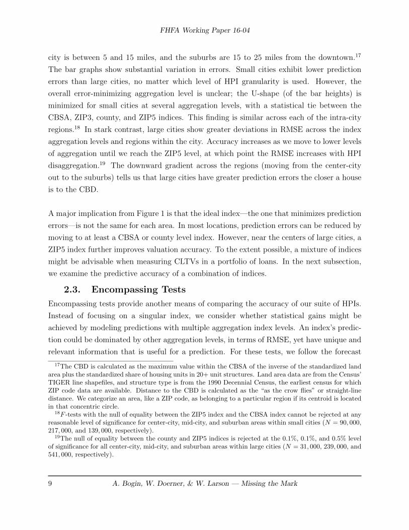
city is between 5 and 15 miles, and the suburbs are 15 to 25 miles from the downtown.17

The bar graphs show substantial variation in errors. Small cities exhibit lower prediction

errors than large cities, no matter which level of HPI granularity is used. However, the

overall error-minimizing aggregation level is unclear; the U-shape (of the bar heights) is

minimized for small cities at several aggregation levels, with a statistical tie between the

CBSA, ZIP3, county, and ZIP5 indices. This finding is similar across each of the intra-city

regions.18 In stark contrast, large cities show greater deviations in RMSE across the index

aggregation levels and regions within the city. Accuracy increases as we move to lower levels

of aggregation until we reach the ZIP5 level, at which point the RMSE increases with HPI

disaggregation.19 The downward gradient across the regions (moving from the center-city

out to the suburbs) tells us that large cities have greater prediction errors the closer a house

is to the CBD.

A major implication from Figure 1 is that the ideal index—the one that minimizes prediction

errors—is not the same for each area. In most locations, prediction errors can be reduced by

moving to at least a CBSA or county level index. However, near the centers of large cities, a

ZIP5 index further improves valuation accuracy. To the extent possible, a mixture of indices

might be advisable when measuring CLTVs in a portfolio of loans. In the next subsection,

we examine the predictive accuracy of a combination of indices.

2.3. Encompassing Tests

Encompassing tests provide another means of comparing the accuracy of our suite of HPIs.

Instead of focusing on a singular index, we consider whether statistical gains might be

achieved by modeling predictions with multiple aggregation index levels. An index’s predic-

tion could be dominated by other aggregation levels, in terms of RMSE, yet have unique and

relevant information that is useful for a prediction. For these tests, we follow the forecast

17The CBD is calculated as the maximum value within the CBSA of the inverse of the standardized landarea plus the standardized share of housing units in 20+ unit structures. Land area data are from the Census’TIGER line shapefiles, and structure type is from the 1990 Decennial Census, the earliest census for whichZIP code data are available. Distance to the CBD is calculated as the “as the crow flies” or straight-linedistance. We categorize an area, like a ZIP code, as belonging to a particular region if its centroid is locatedin that concentric circle.

18F -tests with the null of equality between the ZIP5 index and the CBSA index cannot be rejected at anyreasonable level of significance for center-city, mid-city, and suburban areas within small cities (N = 90, 000,217, 000, and 139, 000, respectively).

19The null of equality between the county and ZIP5 indices is rejected at the 0.1%, 0.1%, and 0.5% levelof significance for all center-city, mid-city, and suburban areas within large cities (N = 31, 000, 239, 000, and541, 000, respectively).



encompassing literature of Chong and Hendry (1986) and Ericsson and Marquez (1993). A

predicted outcome is modeled as a function of a sequence of rival forecasts, i ∈ 1, 2, . . . , I,

at horizon h, such that

Vn,t+h = α0 +I∑i=1

αiVi,n,t+h + en,t+h (7)

where n indicates location and i denotes an index from our suite of geographic aggregation

levels. For interpretation, the constant term, α0, controls for heterogeneity not captured by

the forecasts and de-means the other variables. Parameters α1, . . . , αI indicate the relative

importance of each aggregation level where the information content is conveyed by the sign

and magnitude of the estimated coefficient. If the parameter is not statistically different

than zero, the prediction is “encompassed.” Positive and significant estimates indicate the

presence of unique and relevant information in the forecast. On the other hand, negative

and significant estimates indicate the forecast may be highly collinear with another forecast

and encompassed if the respective index is omitted.20 Each estimated parameter denotes

the fractional amount that it contributes to the prediction. By design, the summation of

the statistically significant and positive parameter estimates should be close to one in a

well-specified model.

20Generally, the omission of the forecast with the negative coefficient should result in either one or morecoefficients decreasing in an equal aggregate magnitude.



Table 2: Index Encompassing Tests

LHS Variable: log House Price

Model (1) (2) (3) (4) (5) (6) (7)Sample Full Rural Small Cities Large Cities Large Cities National HPI National HPI

Center-City Suburbs Growth Decline

National 0.018* -0.127*** -0.010*** 0.066*** 0.031*** -0.069*** 0.155***[0.011] [0.020] [0.003] [0.014] [0.002] [0.002] [0.004]

State 0.001 0.078* -0.012* 0.044 0.025*** 0.016*** 0.028***[0.022] [0.045] [0.007] [0.037] [0.006] [0.005] [0.007]

CBSA -0.004 0.403*** 0.189*** -0.271*** -0.029*** 0.005 -0.006[0.023] [0.053] [0.025] [0.057] [0.011] [0.012] [0.015]

ZIP3 0.145*** 0.072* 0.114*** 0.148* 0.138*** 0.193*** 0.071***[0.018] [0.042] [0.013] [0.088] [0.010] [0.010] [0.012]

County 0.103*** 0.402*** 0.099*** 0.285*** 0.072*** 0.205*** 0.005[0.022] [0.055] [0.025] [0.095] [0.012] [0.013] [0.016]

ZIP5 0.461*** 0.110*** 0.366*** 0.458*** 0.483*** 0.393*** 0.465***[0.012] [0.036] [0.010] [0.036] [0.007] [0.007] [0.009]

Census Tract 0.195*** -0.024 0.177*** 0.152*** 0.198*** 0.168*** 0.210***[0.007] [0.038] [0.009] [0.030] [0.006] [0.006] [0.009]

Census Block Group 0.040*** 0.026 0.036*** 0.051*** 0.043*** 0.036*** 0.041***[0.004] [0.020] [0.005] [0.018] [0.004] [0.004] [0.005]

Constant 0.522*** 0.760*** 0.530*** 0.868*** 0.530*** 0.671*** 0.407***[0.014] [0.022] [0.004] [0.019] [0.003] [0.003] [0.004]

Observations 1,494,788 24,664 486,557 34,048 974,183 1,096,700 398,088R-squared 0.945 0.919 0.94 0.925 0.945 0.935 0.959

Note: *** p < 0.01, ** p < 0.05, * p < 0.1. The unit of observation is a single housing unit transaction. The logof the transaction price is modeled as a function of each index-based estimate. Standard errors are adjusted based onclustering by year × CBSA code. Bold values indicate a statistically significant point estimate greater than 0.15.

We start with the unit of observation being a single housing unit transaction. As with the

RMSE evaluation methods, an initial sale establishes the base price and an index is used

to predict the subsequent sale price of the same unit. This market prediction is used in

Equation 7. Results of index encompassing tests are presented in Table 2 where the actual

value of a housing unit is regressed on a linear function of a constant term and a vector

of forecasts from our suite of HPIs. Each column represents a different sample of housing

transactions to test when the combined information content might be more or less important.

Column 1 gives the full sample of transactions (excluding the first transaction which is used

as the base for the predictions) in the hold-out sample of nearly 1.5 million transactions

where the holding period is 1 year. The ZIP3, county, ZIP5, census tract, and census block

group indices each provide unique and relevant information to the prediction of house prices.

The two most important HPIs (ZIP5 and census tract) are highlighted in bold. A single



index’s estimate does not dominate the others. Rather, similar to Granger and Ramanathan

(1984), a weighted average or a composite index may best predict the price path of individual

housing units.

Columns 2 to 5 depict results for a series of subsamples divided by city size and location. In

rural areas, indices with larger levels of geographic aggregation are preferred.21 The CBSA

and county HPIs are the most relevant, with the ZIP3 and ZIP5 indices contributing less

significantly. Small cities offer a story that begins to emphasize disaggregate indices. As

we move across the columns and city size increases, proximity to the downtown becomes

more important, a result echoed in Bogin, Doerner, and Larson (2016). The ZIP5 HPI is

most influential while census tract and census block group measures contribute additional

information. In general, granular indices are more important for denser areas. More variation

in density amplifies the variation in appreciation rates, which increases the prevalence of bias

when considering larger levels of geographic aggregation.

Finally, in the last two columns, we consider the performance of indices when the national

index is increasing versus decreasing. Column 6 shows that when house prices are rising, a

variety of indices contribute to the optimal composite, with ZIP3, county, ZIP5 and census

tract indices receiving the largest weights. However, when prices fall, the national, ZIP5, and

census tract HPIs exhibit the most explanatory power. The two columns suggest local factors

can drive booms and busts but the national trend becomes an important explanatory aspect

of declines, perhaps because worsening macroeconomic conditions, like financial conditions

and unemployment, are felt everywhere.

Overall, the encompassing tests present a nuanced view of house price index usage. No single

index emerges as the dominate measure. Rather, a weighted average, depending on the area

and condition of the national housing market, could give a superior predictive index. County,

ZIP5, and census tract indices provide the most consistently high levels of predictive power.22

Since submarket indices were also found to be important in the RMSE evaluations, it seems

reasonable that mortgage performance modeling might be improved by using local HPIs to

value houses that serve as collateral. We investigate this conjecture in the next section.

21The “rural” sample is defined as housing units not contained within a CBSA.22While they may be useful in other applications, state-level indices do not appear to provide information

that is not already picked up by the other indices.



3. Modeling Mortgage PerformanceMortgage performance is often modeled in the context of a competing-options framework

where a borrower makes mutually exclusive choices to continue with timely mortgage pay-

ments, prepay a mortgage, or default on the loan (Lawrence and Arshadi, 1995; Deng,

Quigley, and Van Order, 2000; Calhoun and Deng, 2002; Dunsky and Pennington-Cross,

2003; Ergungor and Moulton, 2014). One of the key variables driving borrower behavior in

these models is a mortgage’s loan-to-value (LTV) ratio. Empirical studies find that higher

LTV ratios increase the probability of mortgage default (Schwartz and Torous, 1993; Sher-

lund, 2008; Mayer, Pence, and Sherlund, 2009; Pennington-Cross and Ho, 2010; Bacon and

Moffatt, 2012; Fuster and Willen, 2013; Lam, Dunksy, and Kelly, 2013).23 LTV ratios ex-

ceeding one indicate negative equity, where the borrower is underwater or owes more than

the value of the underlying housing asset. Negative equity can lead homeowners to sig-

nificantly cut back on improvements as well as mortgage principal payments (Olney, 1999;

Melzer, 2013) and substantial evidence indicates borrowers strategically default when houses

go underwater (Deng, Quigley, and Van Order, 2000; Bajari, Chu, and Park, 2008; Bhutta,

Dokko, and Shan, 2010; Ghent and Kudlyak, 2011; Guiso, Sapienza, and Zingales, 2013;

Chan, Haughwout, Hayashi, and van der Klaauw). All of these studies focus on the LTV

ratio, which is composed of two parts—loan amount and house value—both crucial to the

construction of an accurate measure. Loan amount is simple to establish with an actual

payment history or, when unavailable, an amortization table, but market value is not so

easily estimated.

Market value can be estimated in a variety of ways. The LTV at origination is usually based

on a house’s appraisal or sales value. Afterwards, for ongoing analyses, the LTV is updated

with an estimate of current market value, generally derived from observed comparable sales

or statistical modeling.24 The former involves individual expertise, human judgement, and

a forecasting of local market trends but requires considerable time and resources; the latter

uses automated techniques to generate quick and inexpensive estimates but the quality of

the results is largely determined by the richness and accuracy of the underlying property

23Studies find this result with both LTV measured at origination and updated to a current period. Wefocus our attention on latter to examine the combined effect of LTV at origination, principal and interestpayments, and local house price appreciation on the probability of prepayment and default.

24The new ratio is known commonly as the current LTV (CLTV) or marked-to-market LTV (MTMLTV).Although perhaps confusing, the CLTV acronym is sometimes used as a distinct but related shorthand fora combined loan-to-value ratio where a second lien is included in the loan value to measure total leverage.



transactions data. These automated techniques often involve an HPI. Our earlier findings

demonstrate that HPI aggregation can have a meaningful effect on accurate property valu-

ation. Now, we take that one step further by examining whether different levels of accuracy

affect mortgage performance modeling.

We begin this analysis by constructing a model using the variables and techniques commonly

applied in the mortgage finance literature. To do this, we draw from a nationwide sample

of single-family mortgage originations that tracks borrower performance behavior between

1999 and 2014.25 We match identifiers from a stratified random sample of approximately

420,000 loans (35,000 per year) out of 22 million. These 420,000 loans give 1.7 million loan-

year observations. Initially, we estimate the model using CLTV constructed with a national

HPI. Next, we compare actual and predicted rates for prepayment and default across time,

size of city, and location within a city. To investigate the prediction errors, we repeat these

exercises with CLTVs constructed using seven additional HPI measures, each with increasing

geographic granularity. The model and empirical results are presented over the next several

subsections.

3.1. Credit Model

The competing-options framework can be specified formally as a multinomial logit model

with three outcomes, i = {0, 1, 2}, where a borrower remains current, prepays, or defaults

on a mortgage.26 The probability of a borrower choosing an outcome in each period, t, is

Pr(djtz = i) =exp (X ′

jtzβi)

1 +∑2

τ=1 exp (X ′jtzβτ )

(8)

25Public loan origination and performance data are becoming increasingly available. Both Freddie Mac andFannie Mae provide single-family loan-level data going back until 2000 for more than 40 million loans. FreddieMac data are available at http://www.freddiemac.com/news/finance/sf loanlevel dataset.html. The FannieMae data can be found at http://www.fanniemae.com/portal/funding-the-market/data/loan-performance-data.html. The public datasets, though, do not have enough information to reliably identify the propertylocation of individual loans. We obtain a proprietary identifier from Freddie Mac that allows us to matchmortgages across physical addresses and merge information on house price transactions onto the loan per-formance data.

26Other outcomes, like repurchases and proprietary modifications, are possible and do exist in the actualloss sample data that we utilize. However, we focus on borrower behavior and, as is standard practice, weremove terminations that might be triggered by lenders, servicers, or investors.


http://www.freddiemac.com/news/finance/sf_loanlevel_dataset.html

http://www.fanniemae.com/portal/funding-the-market/data/loan-performance-data.html

http://www.fanniemae.com/portal/funding-the-market/data/loan-performance-data.html


Our contribution is analyzing how different measures of CLTV affect predicted outcomes.27

Korteweg and Sorensen (2016) show that current approaches to updating LTV, including the

use of city-level indices, can seriously understate the number of houses that are underwater

by up to 80%, which has been shown to significantly increase the likelihood of default.

Yang, Lin, and Cho (2011) find that not fully accounting for the cross-sectional dispersion

of house prices is a major source of this bias and can significantly affect assessments of

mortgage default risk. Building upon this research, we are particularly interested in how

model accuracy is affected by CLTVs constructed using different levels of HPI granularly.

Our explanatory variables include typical credit model covariates for origination charac-

teristics (e.g., credit score, debt-to-income, loan purpose, number of borrowers), current

performance (e.g., unpaid principal balance, loan age, refinance burnout, yield curve swap

spread, and current loan-to-value), and fixed effects to control for unobserved heterogeneity

(e.g. origination year cohort, state). To remain consistent with earlier sections, we utilize a

20% holdout sample to compare predicted and actual outcomes on observations that have

not been used during model calibration.

3.2. Empirical Results

Results for overall model fit are presented in Figure 2.28 Panels (a), (b), and (c) are based

upon a model using a national HPI to calculate CLTV. Panel (a) illustrates that predicted

and actual rates (of prepayment and default) are relatively close across the last 15 years,

suggesting relative parameter stability across the sample. There are minor deviations when

house prices decline after the housing boom in the early 2000s and again, when prices fell

more drastically, in 2008–2010. To investigate whether disaggregated HPIs might improve

model fit, we examine prediction errors across large and small cities as well as regions within a

city. Prediction errors for prepayments and the geographic patterns are relatively consistent,

with center-city areas having larger prediction errors. In contrast, for defaults, actual and

predicted rates show noticeable differences. Small cities have lower default prediction errors

in center-city regions and larger errors in mid-city and suburban regions. In contrast, large

cities are associated with greater prediction errors in center-city regions. These prediction

errors may partially be a function of measurement error arising from updating CLTVs with

27Given our focus on CLTV, we build and test a model following industry guidance (see Dunsky et al.(2014)). Based upon out-of-sample tests, model fit appears acceptable. By working with a relatively standardmodel, we can focus on CLTV measurement error and its broad effect on model accuracy.

28Because the focus is on improving model fit, individual estimation coefficients are not presented here.



the national HPI.29 Theory suggests measurement error will result in attenuation bias in the

CLTV variable, which we estimate in panels (d) and (e). The graphs show point estimates

for CLTV odds ratios and their confidence intervals constructed with increasingly granular

HPIs. Panel (d) depicts that an increase in CLTV reduces the relative risk of prepayment

but the odds ratio estimate associated with the national index is the smallest (closest to

1). Panel (e) shows the CLTV odds ratio estimates for the default equation. Again, the

estimate associated with the national index is the smallest (closest to 1). The magnitude of

these two sets of coefficients suggests that an accurate CLTV has a larger estimated effect on

default outcomes. This suggests that reducing measurement error will result in a stronger

relationship between CLTV and mortgage performance.

Why might we expect a localized house price measure to improve model fit? House price

appreciation rate gradients have been flat in smalle cities since 1990, but these gradients

have tended to steepen in large cities (Bogin et al., 2016). These gradients are captured by a

national HPI, introducing aggregation bias into CLTV predictions, especially in large cities.

These CLTV errors may harm default model performance. On the other hand, were CLTVs

correlated with other variables in the model, explanatory power may be absorbed by other

parameter estimates, resulting in little net effect.

Our suite of HPIs provide a variety of geographic aggregation levels to estimate the effect of

HPI aggregation on mortgage performance models. To ensure an adequate sample size, we

keep mortgages that fall within metropolitan areas that have at least 10,000 observations.

Based on the property’s location from the CBD, we compare how the choice of HPI gran-

ularity (i.e. a national HPI versus a metro HPI) affects model fit within concentric areas

around the center of a city (e.g., center-city, mid-city, and suburbs). To evaluate model fit,

we compute the RMSE and then consider whether it improves as estimations are performed

with more granular HPIs.

29A larger difference between actual and predicted rates in center-city regions of large cities should notbe surprising. In such places, house price gradients are steeper and are increasing at a faster rate than inareas farther from the CBD. When a single HPI (like a national level) is used, the estimates will tend tounderestimate price levels in center-city areas and over-estimate levels in outskirting areas. More granularHPIs would reduce these errors. Borrowers will realize, too, that their actual house valuation is much higher(or CLTV is lower) and will be less likely to default than may be predicted with a national HPI. Similarly,since center-city areas appreciate at faster rates, refinancing may be more prevalent as borrowers repay to“lock-in” a more favorable rate when leverage is in their favor.



Figure 2: Estimates of Prepayment and Default Model

(a) Comparing Both Outcomes Across Performance Years

0.000

0.006

0.012

0.018

0.024

0.030

0.036

Def

ault

rate

0.00

0.10

0.20

0.30

0.40

0.50

0.60

Prep

aym

ent r

ate

2000

2002

2004

2006

2008

2010

2012

2014

Predicted prepay rate Actual prepay ratePredicted default rate Actual default rate

(b) Prepayments by Location (c) Defaults by Location

0.180

0.200

0.220

mea

n pr

epay

rate

Small City Large CityCenter-City Mid-City Suburbs Center-City Mid-City Suburbs

Actual Predicted

0.008

0.010

0.012

mea

n de

faul

t (D

180)

rate

Small City Large CityCenter-City Mid-City Suburbs Center-City Mid-City Suburbs

Actual Predicted

(d) Prepayment CLTV Attenuation (e) Default CLTV Attenuation

0.991

0.992

0.993

0.994

0.995

CLT

V o

dds

ratio

Block

Tract

ZIP5

County ZIP

3Metr

oStat

eNatl

Index geographic aggregation level

1.030

1.032

1.034

1.036

1.038

CLT

V o

dds

ratio

Block

Tract

ZIP5

County ZIP

3Metr

oStat

eNatl



FHFA

Work

ingPap

er16-04

Figure 3: Comparing Fit by HPI Granularity and Region Within a City

(a) Entire Sample

0.0049

0.0050

0.0051

0.0052

0.0053

0.0054

RM

SE

of D

efau

lts

0.0522

0.0524

0.0526

0.0528

0.0530

RM

SE

of P

repa

ymen

ts

Block

Tract

ZIP5

County ZIP

3

Metro

State

Natl


Prepay RMSE Default RMSE

(b) Center-City (c) Mid-City (d) Suburbs

0.0055

0.0056

0.0057

0.0058

0.0059

0.0060

RM

SE

of D

efau

lts

0.0550

0.0555

0.0560

0.0565

RM

SE

of P

repa

ymen

ts

Block

Tract

ZIP5

County ZIP

3

Metro

State

Natl



0.0050

0.0052

0.0054

0.0056

0.0058

RM

SE

of D

efau

lts

0.0522

0.0523

0.0524

0.0525

0.0526

0.0527

RM

SE

of P

repa

ymen

ts

Block

Tract

ZIP5

County ZIP

3

Metro

State

Natl



0.0053

0.0054

0.0055

0.0056

0.0057

0.0058

RM

SE

of D

efau

lts

0.0530

0.0532

0.0534

0.0536

0.0538

RM

SE

of P

repa

ymen

ts

Block

Tract

ZIP5

County ZIP

3

Metro

State

Natl



Note: Mean values, of actual prepayments and defaults, and predictions are computed within performance year and for each region within acity that has at least 10,000 observations in our holdout sample (the four panels shown above). Statistical significance (per a F -distribution)is computed by taking the ratio of the RMSE of an HPI granularity level compared to the RMSE for the national HPI. Geometric shapesillustrate when a more granular HPI improves model fit (i.e., a triangle for p ≤ 0.01, a circle for 0.05, and a square for 0.10).

18A.Bog

in,W

.Doern

er,&

W.Larson

—Missin

gtheMark


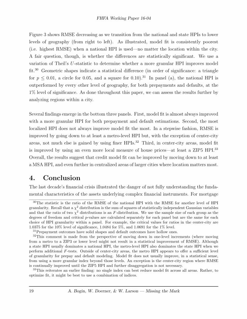
Figure 3 shows RMSE decreasing as we transition from the national and state HPIs to lower

levels of geography (from right to left). As illustrated, model fit is consistently poorest

(i.e. highest RMSE) when a national HPI is used—no matter the location within the city.

A fair question, though, is whether the differences are statistically significant. We use a

variation of Theil’s U -statistic to determine whether a more granular HPI improves model

fit.30 Geometric shapes indicate a statistical difference (in order of significance: a triangle

for p ≤ 0.01, a circle for 0.05, and a square for 0.10).31 In panel (a), the national HPI is

outperformed by every other level of geography, for both prepayments and defaults, at the

1% level of significance. As done throughout this paper, we can assess the results further by

analyzing regions within a city.

Several findings emerge in the bottom three panels. First, model fit is almost always improved

with a more granular HPI for both prepayment and default estimations. Second, the most

localized HPI does not always improve model fit the most. In a stepwise fashion, RMSE is

improved by going down to at least a metro-level HPI but, with the exception of center-city

areas, not much else is gained by using finer HPIs.32 Third, in center-city areas, model fit

is improved by using an even more local measure of house prices—at least a ZIP5 HPI.33

Overall, the results suggest that credit model fit can be improved by moving down to at least

a MSA HPI, and even further in centralized areas of larger cities where location matters most.

4. ConclusionThe last decade’s financial crisis illustrated the danger of not fully understanding the funda-

mental characteristics of the assets underlying complex financial instruments. For mortgage

30The statistic is the ratio of the RMSE of the national HPI with the RMSE for another level of HPIgranularity. Recall that a χ2 distribution is the sum of squares of statistically independent Gaussian variablesand that the ratio of two χ2 distributions is an F -distribution. We use the sample size of each group as thedegrees of freedom and critical p-values are calculated separately for each panel but are the same for eachchoice of HPI granularity within a panel. For example, the critical values for ratios in the center-city are1.0375 for the 10% level of significance, 1.0484 for 5%, and 1.0691 for the 1% level.

31Prepayment outcomes have solid shapes and default outcomes have hollow ones.32This comment is made from the perspective of moving down in one-level increments (where moving

from a metro to a ZIP3 or lower level might not result in a statistical improvement of RMSE). Althougha state HPI usually dominates a national HPI, the metro-level HPI also dominates the state HPI when weperform additional F -tests. Outside of center-city areas, the metro HPI appears to offer a sufficient levelof granularity for prepay and default modeling. Model fit does not usually improve, in a statistical sense,from using a more granular index beyond those levels. An exception is the center-city region where RMSEis continually improved until the ZIP5 HPI and further disaggregation is not necessary.

33This reiterates an earlier finding: no single index can best reduce model fit across all areas. Rather, tooptimize fit, it might be best to use a combination of indices.



backed securities, an important feature of the mortgage collateral is the location of the prop-

erties in the reference pool. In this paper, we offer new evidence that the geographic scope of

house price indices can affect price valuations and mortgage performance modeling for such

collateral.

We find that local constant-quality HPIs capture within-city heterogeneity of house price

levels and appreciation rates, which can compound over time, particularly in the center-

cities of large cities. This known heterogeneity means that less granular indices (i.e., ZIP3,

state, or national HPIs) can lead to market value errors that are predictable spatially, as a

function of distance to the central business district (CBD), and the errors can be non-trivial.

The consequences of geographic aggregation hinge on the relative steepness of house price

gradients within an area: in large cities with steep gradients, aggregation has substantial

costs, but in smaller or more supply-elastic cities, aggregation is relatively benign.

We also find that CLTVs estimated using local HPIs result in lower prepayment and de-

fault rate model errors relative to models using CLTVs estimated using state or national

HPIs. The results suggest that CLTVs constructed using more aggregated HPIs tend to

capture general trends in borrower equity, but with substantial remaining error. The bene-

fits of disaggregation are most striking near the centers of large cities, where performance is

substantially improved by estimating CLTVs using a ZIP code index.34

Overall, the realtors’ mantra of “location, location, location” is apparently true as location

seems to have important implications for housing finance. A mortgage’s value at origination

and ongoing loan performance are often more accurately measured with a local HPI. Our

analysis suggests this is particularly true in larger cities, where results are most sensitive to

the choice of a house price index and the effect of “missing the mark”.

ReferencesAlonso, W. (1964). Location and land use: Toward a general theory of land rent. Harvard

University Press.

Andersson, F. and Mayock, T. (2014). Loss severities on residential real estate debt during

34Although beyond the scope of this paper, this within-city evidence of local house price appreciation hasimplications for risk-return tradeoffs. Han (2013) finds cities with inelastic housing and growing populationstend to have strong hedging incentives. Our results suggest these effects might be further magnified incentralized areas within larger cities.



the great recession. Journal of Banking & Finance, 46:266–284.

Bacon, P. M. and Moffatt, P. G. (2012). Mortgage choice as a natural field experiment onchoice under risk. Journal of Money, Credit and Banking, 44(7):1401–1426.

Bailey, M. J., Muth, R. F., and Nourse, H. O. (1963). A regression method for real estateprice index construction. Journal of the American Statistical Association, 58(304):933–942.

Bajari, P., Chu, S., and Park, M. (2008). An empirical model of subprime mortgage defaultfrom 2000 to 2007. Working Paper Series 14625, National Bureau of Economic Research.

Bhutta, N., Dokko, J., and Shan, H. (2010). The depth of negative equity and mortgagedefault decisions. Finance and Economics Discussion Series, Working Paper 2010-35,Board of Governors of the Federal Reserve System.

Bogin, A. N., Doerner, W. M., and Larson, W. D. (2016). Local house price dynamics: Newindices and stylized facts. Working Paper Series 16-01, Federal Housing Finance Agency.

Calhoun, C. A. and Deng, Y. (2002). A dynamic analysis of fixed-and adjustable-rate mort-gage terminations. Journal of Real Estate Finance and Economics, 24(1-2):9–33.

Case, K. E. and Shiller, R. J. (1987). Prices of single-family homes since 1970: New indexesfor four cities. New England Economic Review, Sep/Oct:45–56.

Chan, S., Haughwout, A., Hayashi, A., and van der Klaauw, W. (2016). Determinants ofmortgage default and consumer credit use: The effects of foreclosure laws and foreclosuredelays. Journal of Money, Credit and Banking, 48(2-3):393–413.

Chong, Y. Y. and Hendry, D. F. (1986). Econometric evaluation of linear macro-economicmodels. The Review of Economic Studies, 53(4):671–690.

Deng, Y., Quigley, J. M., and Van Order, R. (2000). Mortgage terminations, heterogeneityand the exercise of mortgage options. Econometrica, 68(2):275–307.

Dunsky, R. M. and Pennington-Cross, A. (2003). Estimation, deployment and backtesting ofdefault, prepayment equations. Working paper series, Office of Federal Housing EnterpriseOversight.

Dunsky, R. M., Zhou, X., Kane, M., Chow, M., Hu, C., and Varrieur, A. (2014). FHFAMortgage Analytics Platform. Working paper series, Federal Housing Finance Agency.

Ergungor, O. E. and Moulton, S. (2014). Beyond the transaction: Banks and mortgagedefault of low-income homebuyers. Journal of Money, Credit and Banking, 46(8):1721–1752.

Ericsson, N. R. and Marquez, J. (1993). Encompassing the forecasts of U.S. trade balancemodels. The Review of Economics and Statistics, 75(1):19–31.



Fuster, A. and Willen, P. S. (2013). Payment size, negative equity, and mortgage default.Working Paper Series 19345, National Bureau of Economic Research.

Ghent, A. C. and Kudlyak, M. (2011). Recourse and residential mortgage default: Evidencefrom US states. Review of Financial Studies, 24(9):3139–3186.

Granger, C. W. and Ramanathan, R. (1984). Improved methods of combining forecasts.Journal of Forecasting, 3(2):197–204.

Guiso, L., Sapienza, P., and Zingales, L. (2013). The determinants of attitudes towardstrategic default on mortgages. The Journal of Finance, 68(4):1473–1515.

Han, L. (2013). Understanding the puzzling risk-return relationship for housing. Review ofFinancial Studies, 26(4):877–928.

Korteweg, A. and Sorensen, M. (2016). Estimating loan-to-value distributions. Real EstateEconomics, 44(1):1–46.

Lam, K., Dunksy, R. M., and Kelly, A. (2013). Impacts of down payment underwritingstandards on loan performance—evidence from the GSEs and FHA portfolios. WorkingPaper Series 13-03, Federal Housing Finance Agency.

Lawrence, E. C. and Arshadi, N. (1995). A multinomial logit analysis of problem loanresolution choices in banking. Journal of Money, Credit and Banking, 27(1):202–216.

Mayer, C., Pence, K., and Sherlund, S. M. (2009). The rise in mortgage defaults. TheJournal of Economic Perspectives, 23(1):27–50.

Melzer, B. T. (2013). Mortgage debt overhang: Reduced investment by homeowners withnegative equity. Working paper series, Northwestern University.

Mills, E. S. (1967). An aggregative model of resource allocation in a metropolitan area.American Economic Review, 57(2):197–210.

Muth, R. F. (1969). Cities and Housing; the Spatial Pattern of Urban Residential Land Use.University of Chicago Press.

Nagaraja, C., Brown, L., and Wachter, S. (2014). Repeat sales house price index methodol-ogy. Journal of Real Estate Literature, 22(1):23–46.

Olney, M. L. (1999). Avoiding default: The role of credit in the consumption collapse of1930. Quarterly Journal of Economics, 114(1):319–335.

Pennington-Cross, A. and Ho, G. (2010). The termination of subprime hybrid and fixed-ratemortgages. Real Estate Economics, 38(3):399–426.

Schwartz, E. S. and Torous, W. N. (1993). Mortgage prepayment and default decisions: APoisson regression approach. Real Estate Economics, 21(4):431–449.



Sherlund, S. M. (2008). The past, present, and future of subprime mortgages. Finance andEconomics Discussion Series, Working Paper 2008-63, Board of Governors of the FederalReserve System.

Stroebel, J. (2016). Asymmetric information about collateral values. The Journal of Finance,71(3):1071–1111.

Theil, H. (1966). Applied Economic Forecasting. North-Holland Publishing Company, Am-sterdam.

Yang, T. T., Lin, C.-C., and Cho, M. (2011). Collateral risk in residential mortgage defaults.The Journal of Real Estate Finance and Economics, 42(2):115–142.


Date post:	24-Jul-2018
Category:	Documents
Upload:	nguyentu
View:	215 times
Download:	0 times

Alexander N. Bogin William M. Doerner William D. Larson ... · Missing the Mark: House Price Index...

Documents