Algebra Introduction to Conic Sections The intersection of a cone and a plane is called a conic section. There are four types of curves that result from these intersections that are of particular interest: Parabola Circle Ellipse Hyperbola Each of these has a geometric definition, from which the algebraic form is derived. Geometric Definitions Parabola – The set of all points that are the same distance from a point (called the focus) and a line (called the Directrix). Ellipse – The set of all points for which the sum of the distances to two points (called foci) is constant. Circle – The set of all points that are the same distance from a point (called the center). The distance is called the radius. Hyperbola – The set of all points for which the difference of the distances to two points (called foci) is constant. Page 1 of 15
Transcript
Algebra
Introduction to Conic Sections The intersection of a cone and a plane is called a conic section. There are four types of curves that result from these intersections that are of particular interest:
Parabola
Circle
Ellipse
Hyperbola
Each of these has a geometric definition, from which the algebraic form is derived.
Geometric Definitions
Parabola – The set of all points that are the same distance from a point (called the focus) and a line (called the Directrix).
Ellipse – The set of all points for which the sum of the distances to two points (called foci) is constant.
Circle – The set of all points that are the same distance from a point (called the center). The distance is called the radius.
Hyperbola – The set of all
points for which the
difference of the distances to two points (called foci) is
constant.
Page 1 of 15
Algebra
Parabola with Vertex at the Origin (Standard Position)
Horizontal Directrix Vertical Directrix
Characteristics of a Parabola in Standard Position
Horizontal Directrix Vertical Directrix
Equation 4 4
If 0 opens up opens right
If 0 opens down opens left
Eccentricity (“e”) 1 1
Value of p (in illustration) 1 1
Vertex 0, 0 ‐ the origin 0, 0 ‐ the origin
Focus 0, , 0
Directrix
Axis of symmetry 0 (y‐axis) 0 (x‐axis)
4 4
Page 2 of 15
Algebra
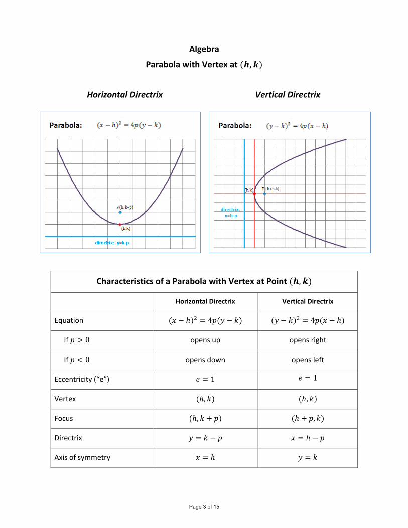
Parabola with Vertex at ,
Horizontal Directrix Vertical Directrix
Characteristics of a Parabola with Vertex at Point ,
Horizontal Directrix Vertical Directrix
Equation 4 4
If 0 opens up opens right
If 0 opens down opens left
Eccentricity (“e”) 1 1
Vertex , ,
Focus , ,
Directrix
Axis of symmetry
Page 3 of 15
Algebra
Parabola in Polar Form
Horizontal Directrix Vertical Directrix
Characteristics of a Parabolas in Polar Form
Horizontal Directrix Vertical Directrix
Equation (simplified) 1 sin
1 cos
If " " in denominator opens up
Directrix below Pole
opens right
Directrix left of Pole
If " " in denominator opens down
Directrix above Pole
opens left
Directrix right of Pole
Eccentricity (“e”) 1 1
Focal Parameter (“p”) distance between the Directrix and the Focus
Note: “p” in Polar Form is different from “p” in Cartesian Form
Coordinates of Key Points: (change all instances of “–p” below to “p” if “+” is in the denominator)
Vertex 0, /2 /2, 0
Focus 0,0 0,0)
Directrix
Page 4 of 15
Algebra Circles
Characteristics of a Circle
in Standard Position
Equation
Center 0,0 ‐ the origin
Radius
In the example 4
Characteristics of a Circle
in Polar Form
Equation
Pole 0, 0
Radius
Characteristics of a Circle
Centered at Point (h, k)
Equation
Center ,
Radius
Page 5 of 15
Algebra Ellipse Centered on the Origin (Standard Position)
Vertical Major Axis
Horizontal Major Axis
Characteristics of an Ellipse in Standard Position
Horizontal Major Axis Vertical Major Axis
In the above example 5, 4, 3 5, 4, 3
Equation 1 1
Values of " " and " "
Value of " "
Eccentricity (“e”) / 0 1
Center 0,0 ‐ the origin
Major Axis Vertices , 0 0,
Minor Axis Vertices 0, , 0
Foci , 0 0,
Directrixes (not shown) / /
Page 6 of 15
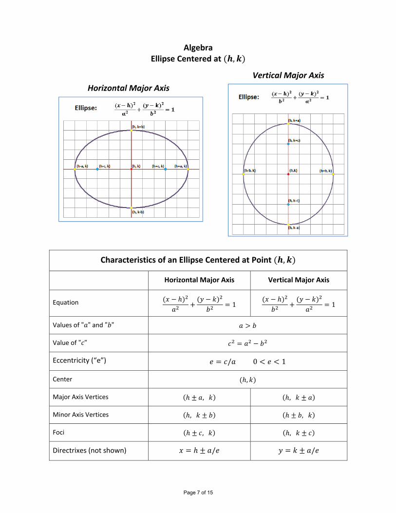
Algebra Ellipse Centered at ,
Vertical Major Axis
Horizontal Major Axis
Characteristics of an Ellipse Centered at Point ,
Horizontal Major Axis Vertical Major Axis
Equation 1 1
Values of " " and " "
Value of " "
Eccentricity (“e”) / 0 1
Center ,
Major Axis Vertices , ,
Minor Axis Vertices , ,
Foci , ,
Directrixes (not shown) / /
Page 7 of 15
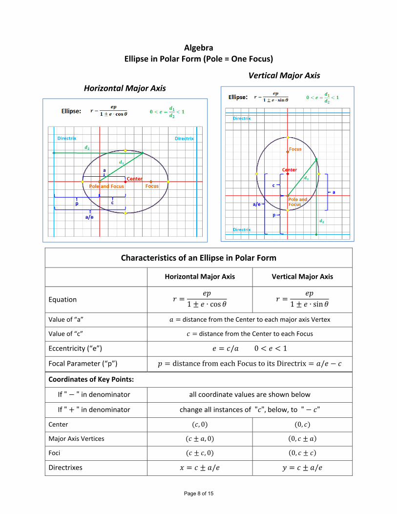
Algebra Ellipse in Polar Form (Pole = One Focus)
Vertical Major Axis
Horizontal Major Axis
Characteristics of an Ellipse in Polar Form
Horizontal Major Axis Vertical Major Axis
Equation 1 ∙ cos
1 ∙ sin
Value of “a” distance from the Center to each major axis Vertex
Value of “c” distance from the Center to each Focus
Eccentricity (“e”) / 0 1
Focal Parameter (“p”) distance from each Focus to its Directrix /
Coordinates of Key Points:
If " " in denominator all coordinate values are shown below
If " " in denominator change all instances of " ", below, to " "
Center , 0 0,
Major Axis Vertices , 0 0,
Foci , 0 0,
Directrixes / /
Page 8 of 15
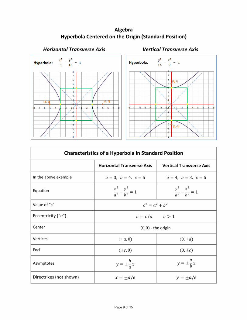
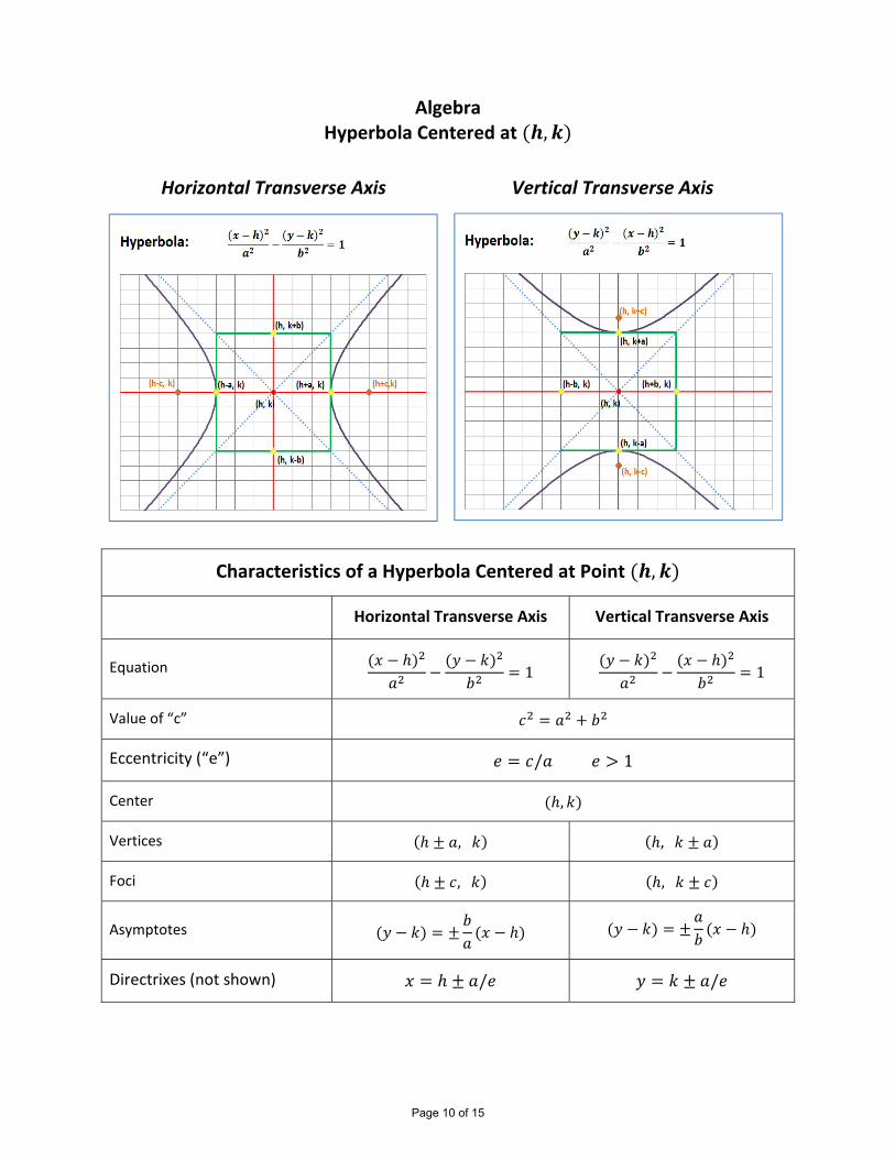
Algebra Hyperbola Centered on the Origin (Standard Position)
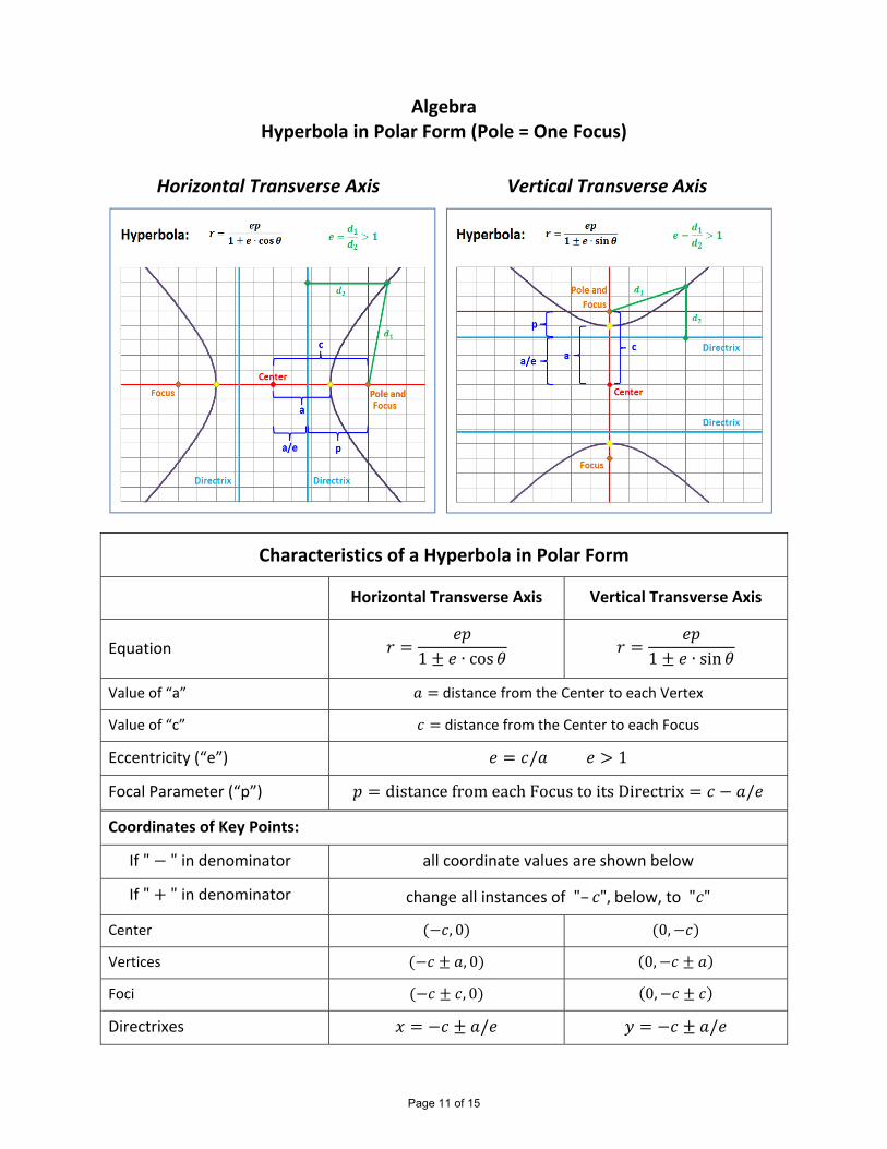
Value of “a” distance from the Center to each Vertex
Value of “c” distance from the Center to each Focus
Eccentricity (“e”) / 1
Focal Parameter (“p”) distance from each Focus to its Directrix /
Coordinates of Key Points:
If " " in denominator all coordinate values are shown below
If " " in denominator change all instances of "– ", below, to " "
Center , 0 0,
Vertices , 0 0,
Foci , 0 0,
Directrixes / /
Page 11 of 15
Algebra Hyperbola in Polar Form (Pole = One Focus)
Partial Construction Over the Domain: to
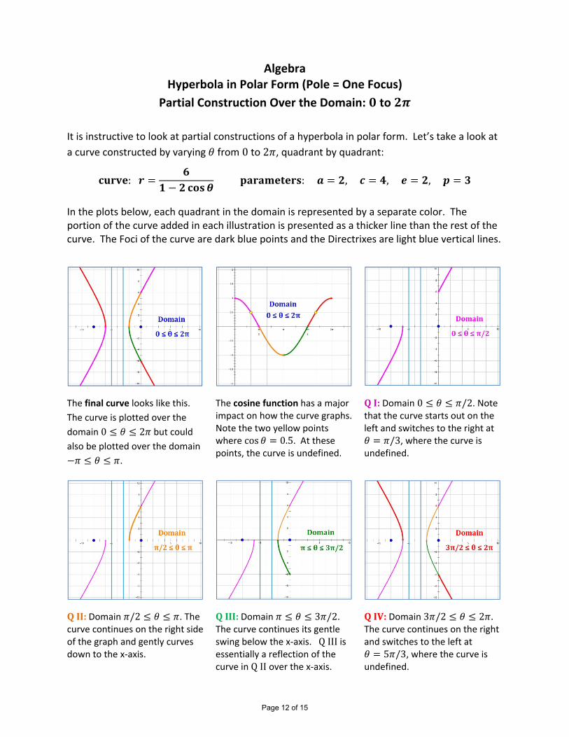
It is instructive to look at partial constructions of a hyperbola in polar form. Let’s take a look at
a curve constructed by varying from 0 to 2 , quadrant by quadrant:
: : , , ,
In the plots below, each quadrant in the domain is represented by a separate color. The portion of the curve added in each illustration is presented as a thicker line than the rest of the curve. The Foci of the curve are dark blue points and the Directrixes are light blue vertical lines.
The final curve looks like this.
The curve is plotted over the
domain 0 2 but could
also be plotted over the domain
.
The cosine function has a major impact on how the curve graphs. Note the two yellow points where cos 0.5. At these points, the curve is undefined.
QI: Domain 0 /2. Note that the curve starts out on the left and switches to the right at
/3, where the curve is undefined.
QII: Domain /2 . The curve continues on the right side of the graph and gently curves down to the x‐axis.
QIII: Domain 3 /2. The curve continues its gentle swing below the x‐axis. QIII is essentially a reflection of the curve in QII over the x‐axis.
QIV: Domain 3 /2 2 . The curve continues on the right and switches to the left at
5 /3, where the curve is undefined.
Page 12 of 15
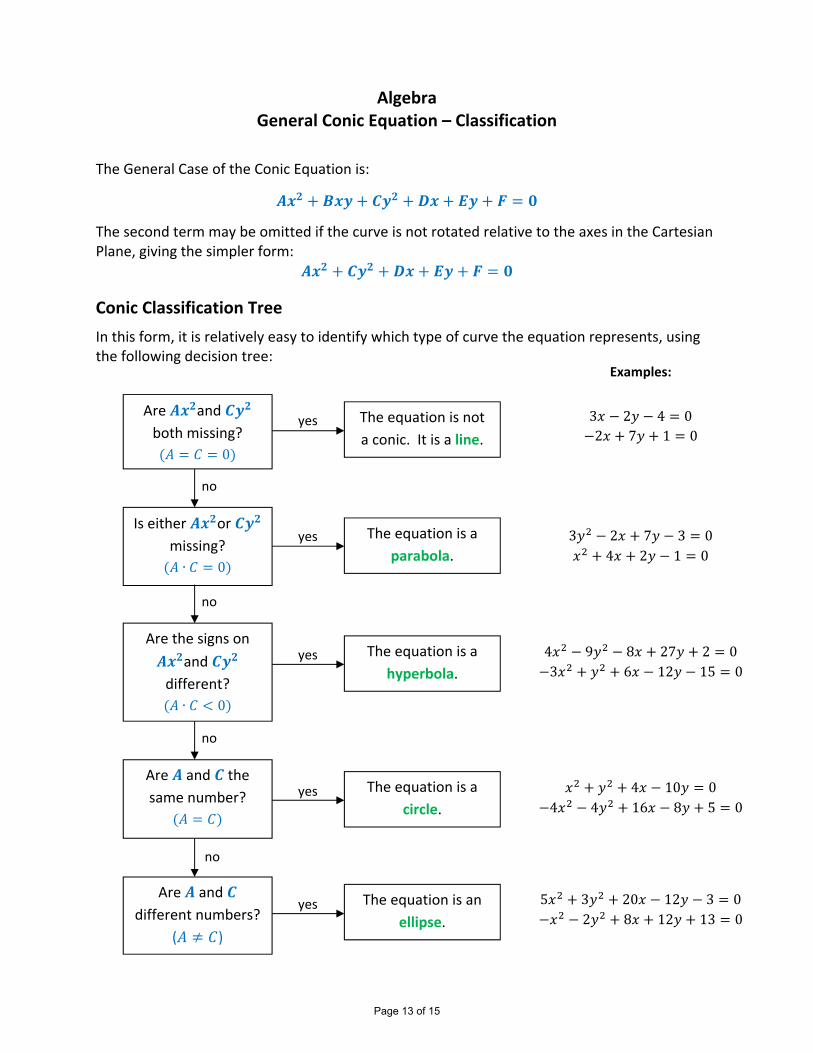
Examples:
3 2 4 0 2 7 1 0
3 2 7 3 0 4 2 1 0
4 9 8 27 2 0 3 6 12 15 0
4 10 0 4 4 16 8 5 0
5 3 20 12 3 0 2 8 12 13 0
Algebra General Conic Equation – Classification
The General Case of the Conic Equation is:
The second term may be omitted if the curve is not rotated relative to the axes in the Cartesian Plane, giving the simpler form:
Conic Classification Tree
In this form, it is relatively easy to identify which type of curve the equation represents, using the following decision tree:
no
no
no
yes
no
yes
0
Are and
both missing? The equation is not
a conic. It is a line.
Are and
different numbers?
( )
Are and the
same number?
∙ 0
Are the signs on
and
different?
∙ 0
Is either or
missing? The equation is a
parabola.
The equation is a
hyperbola.
The equation is a
circle.
The equation is an
ellipse.
yes
yes
yes
Page 13 of 15
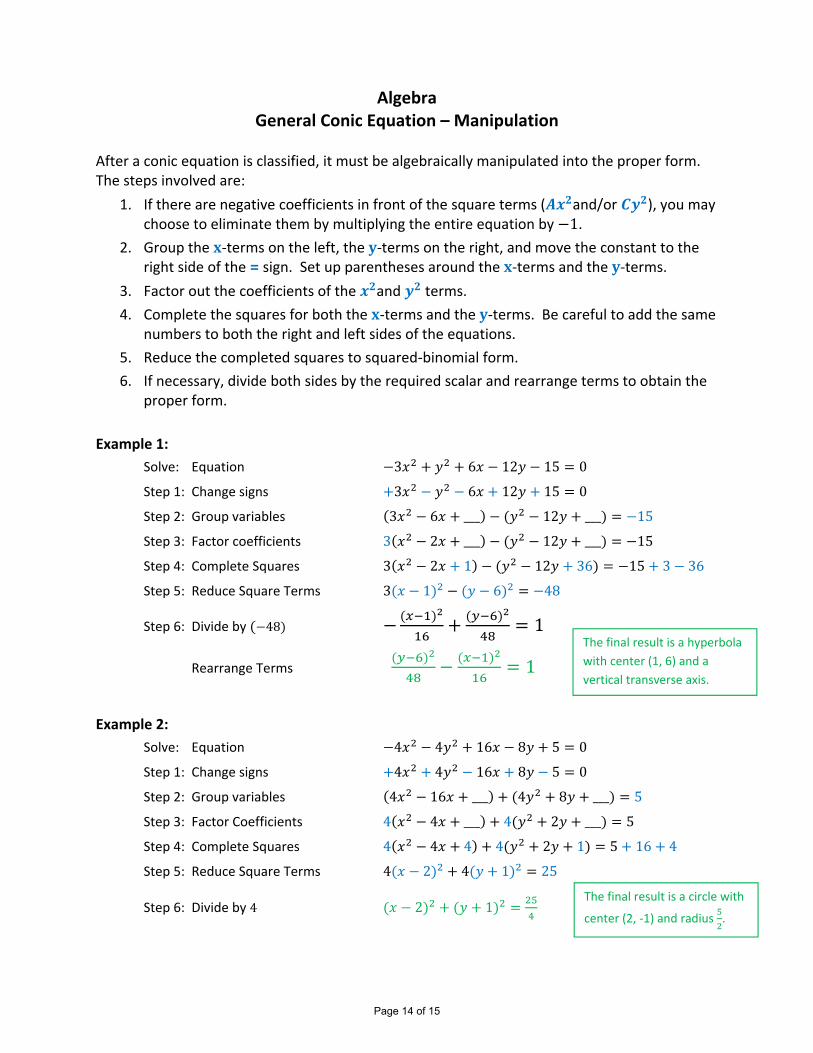
Algebra General Conic Equation – Manipulation
After a conic equation is classified, it must be algebraically manipulated into the proper form. The steps involved are:
1. If there are negative coefficients in front of the square terms ( and/or ), you may choose to eliminate them by multiplying the entire equation by 1.
2. Group the x‐terms on the left, the y‐terms on the right, and move the constant to the right side of the = sign. Set up parentheses around the x‐terms and the y‐terms.
3. Factor out the coefficients of the and terms.
4. Complete the squares for both the x‐terms and the y‐terms. Be careful to add the same numbers to both the right and left sides of the equations.
5. Reduce the completed squares to squared‐binomial form.
6. If necessary, divide both sides by the required scalar and rearrange terms to obtain the proper form.


![[LEC]1.2 Conic Sections](https://static.documents.pub/doc/80x56/577d2eb01a28ab4e1eafbd09/lec12-conic-sections.jpg)


