178
Copyright 2008‐13, Earl Whitney, Reno NV. All Rights Reserved Math Handbook of Formulas, Processes and Tricks Algebra Prepared by: Earl L. Whitney, FSA, MAAA Version 2.5 April 2, 2013
| Date post: | 04-Jun-2018 |
| Category: |
Documents |
| Upload: | jmagomedov723730930 |
| View: | 218 times |
| Download: | 0 times |

8/13/2019 AlgebraHandbook_very Helpful_ Print It
http://slidepdf.com/reader/full/algebrahandbookvery-helpful-print-it 1/178
Copyright 2008‐13, Earl Whitney, Reno NV. All Rights Reserved
Math Handbook of Formulas, Processes and Tricks
Algebra
Prepared by: Earl L. Whitney, FSA, MAAA Version 2.5 April 2, 2013

8/13/2019 AlgebraHandbook_very Helpful_ Print It
http://slidepdf.com/reader/full/algebrahandbookvery-helpful-print-it 2/178
Page Description
Chapter 1: Basics
9 Order of Operations (PEMDAS, Parenthetical Device)
10 Graphing with Coordinates (Coordinates, Plotting Points)
11 Linear Patterns (Recognition, Converting to an Equation)
12 Identifying Number Patterns
13 Completing Number Patterns
14 Basic Number Sets (Sets of Numbers, Basic Number Set Tree)
Chapter 2: Operations
15 Operating with Real Numbers (Absolute Value, Add, Subtract, Multiply, Divide)
16 Properties of Algebra (Addition & Multiplication, Zero, Equality)
Chapter 3: Solving Equations
18 Solving Multi‐Step Equations
19 Tips and Tricks in Solving Multi‐Step Equations
Chapter 4: Probability & Statistics
20 Probability and Odds
21 Probability with Dice
22 Combinations
23 Statistical Measures
Chapter 5: Functions
24 Introduction to Functions (Definitions, Line Tests)
25 Special Integer Functions
26 Operations with Functions
27 Composition of Functions
28 Inverses of Functions
29 Transformation – Translation
30 Transformation – Vertical Stretch and Compression
31 Transformation – Horizontal Stretch and Compression
32 Transformation – Reflection
33 Transformation – Summary
34 Building a Graph with Transformations
Algebra Handbook Table of Contents
-2-
Version 2.5 4/2/2013

8/13/2019 AlgebraHandbook_very Helpful_ Print It
http://slidepdf.com/reader/full/algebrahandbookvery-helpful-print-it 3/178
Algebra Handbook Table of Contents
Page Description
Chapter 6: Linear Functions
35 Slope of a Line (Mathematical Definition)
36 Slope of a Line (Rise over Run)
37 Slopes of Various Lines (8 Variations)
38 Various Forms of a Line (Standard, Slope‐Intercept, Point‐Slope)
39 Slopes of Parallel and Perpendicular Lines
40 Parallel, Perpendicular or Neither
41 Parallel, Coincident or Intersecting
Chapter 7: Inequalities
42 Properties of Inequality43 Graphs of Inequalities in One Dimension
44 Compound Inequalities in One Dimension
45 Inequalities in Two Dimensions
46 Graphs of Inequalities in Two Dimensions
47 Absolute Value Functions (Equations)
48 Absolute Value Functions (Inequalities)
Chapter 8: Systems of Equations
49 Graphing a Solution
50 Substitution Method
51 Elimination Method
52 Classification of Systems of Equations
53 Linear Dependence
54 Systems of Inequalities in Two Dimensions
55 Parametric Equations
Chapter 9: Exponents (Basic) and Scientific Notation
56 Exponent Formulas
57 Scientific Notation (Format, Conversion)
58 Adding and Subtracting with Scientific Notation
59 Multiplying and Dividing with Scientific Notation
-3-
Version 2.5 4/2/2013

8/13/2019 AlgebraHandbook_very Helpful_ Print It
http://slidepdf.com/reader/full/algebrahandbookvery-helpful-print-it 4/178
Algebra Handbook Table of Contents
Page Description
Chapter 10: Polynomials – Basic
60 Introduction to Polynomials
61 Adding and Subtracting Polynomials
62 Multiplying Binomials (FOIL, Box, Numerical Methods)
63 Multiplying Polynomials
64 Dividing Polynomials
65 Factoring Polynomials
66 Special Forms of Quadratic Functions (Perfect Squares)
67 Special Forms of Quadratic Functions (Differences of Squares)
68 Factoring Trinomials – Simple Case Method
69 Factoring Trinomials – AC Method70 Factoring Trinomials – Brute Force Method
71 Factoring Trinomials – Quadratic Formula Method
72 Solving Equations by Factoring
Chapter 11: Quadratic Functions
73 Introduction to Quadratic Functions
74 Completing the Square
75 Table of Powers and Roots
76 The Quadratic Formula
77 Quadratic Inequalities in One Variable
79 Fitting a Quadratic through Three Points
Chapter 12: Complex Numbers
80 Complex Numbers ‐ Introduction
81 Operations with Complex Numbers
82 The Square Root of i
83 Complex Numbers – Graphical Representation
84 Complex Number Operations in Polar Coordinates
85 Complex Solutions to Quadratic Equations
-4-
Version 2.5 4/2/2013

8/13/2019 AlgebraHandbook_very Helpful_ Print It
http://slidepdf.com/reader/full/algebrahandbookvery-helpful-print-it 5/178
Algebra Handbook Table of Contents
Page Description
Chapter 13: Radicals
86 Radical Rules
87 Simplifying Square Roots (Extracting Squares, Extracting Primes)
88 Solving Radical Equations
89 Solving Radical Equations (Positive Roots, The Missing Step)
Chapter 14: Matrices
90 Addition and Scalar Multiplication
91 Multiplying Matrices
92 Matrix Division and Identity Matrices
93 Inverse of a 2x2 Matrix94 Calculating Inverses – The General Case (Gauss‐Jordan Elimination)
95 Determinants – The General Case
96 Cramer’s Rule – 2 Equations
97 Cramer’s Rule – 3 Equations
98 Augmented Matrices
99 2x2 Augmented Matrix Examples
100 3x3 Augmented Matrix Example
Chapter 15: Exponents and Logarithms
101 Exponent Formulas
102 Logarithm Formulas
103 e
104 Table of Exponents and Logs
105 Converting Between Exponential and Logarithmic Forms
106 Expanding Logarithmic Expressions
107 Condensing Logarithmic Expressions
108 Condensing Logarithmic Expressions – More Examples
109 Graphing an Exponential Function
110 Four Exponential Function Graphs
111 Graphing a Logarithmic Function
114 Four Logarithmic Function Graphs
115 Graphs of Various Functions
116 Applications of Exponential Functions (Growth, Decay, Interest)
117 Solving Exponential and Logarithmic Equations
-5-
Version 2.5 4/2/2013

8/13/2019 AlgebraHandbook_very Helpful_ Print It
http://slidepdf.com/reader/full/algebrahandbookvery-helpful-print-it 6/178
Algebra Handbook Table of Contents
Page Description
Chapter 16: Polynomials – Intermediate
118 Polynomial Function Graphs
119 Finding Extrema with Derivatives
120 Factoring Higher Degree Polynomials – Sum and Difference of Cubes
121 Factoring Higher Degree Polynomials – Variable Substitution
122 Factoring Higher Degree Polynomials – Synthetic Division
123 Comparing Synthetic Division and Long Division
124 Zeros of Polynomials – Developing Possible Roots
125 Zeros of Polynomials – Testing Possible Roots
126 Intersections of Curves (General Case, Two Lines)
127 Intersections of Curves (a Line and a Parabola)128 Intersections of Curves (a Circle and an Ellipse)
Chapter 17: Rational Functions
129 Domains of Rational Functions
130 Holes and Asymptotes
131 Graphing Rational Functions
131 Simple Rational Functions
132 Simple Rational Functions ‐Example
133 General Rational Functions
135 General Rational Functions ‐Example
137 Operating with Rational Expressions
138 Solving Rational Equations
139 Solving Rational Inequalities
Chapter 18: Conic Sections
140 Introduction to Conic Sections
141 Parabola with Vertex at the Origin (Standard Position)
142 Parabola with Vertex at Point h, k
143 Parabola in Polar Form
144 Circles
145 Ellipse Centered on the Origin (Standard Position)
146 Ellipse Centered at Point (h, k)
147 Ellipse in Polar Form
148 Hyperbola Centered on the Origin (Standard Position)
149 Hyperbola Centered at Point (h, k)
150 Hyperbola in Polar Form
151 Hyperbola Construction Over the Domain: 0 to 2π
152 General Conic Equation ‐Classification
153 General Conic Formula – Manipulation (Steps, Examples)
154 Parametric Equations of Conic Sections
-6-
Version 2.5 4/2/2013

8/13/2019 AlgebraHandbook_very Helpful_ Print It
http://slidepdf.com/reader/full/algebrahandbookvery-helpful-print-it 7/178
Algebra Handbook Table of Contents
Page Description
Chapter 19: Sequences and Series
155 Introduction to Sequences and Series
156 Fibonacci Sequence
157 Summation Notation and Properties
158 Some Interesting Summation Formulas
159 Arithmetic Sequences
160 Arithmetic Series
161 Pythagorean Means (Arithmetic, Geometric)
162 Pythagorean Means (Harmonic)
163 Geometric Sequences
164 Geometric Series165 A Few Special Series (π, e, cubes)
166 Pascal’s Triangle
167 Binomial Expansion
168 Gamma Function and n !
169 Graphing the Gamma Function
170 Index
Useful Websites
http://www.mathguy.us/
http://mathworld.wolfram.com/
http://www.purplemath.com/
http://www.math.com/homeworkhelp/Algebra.html
Wolfram Math World – Perhaps the premier site for mathematics on the Web. This site contains
definitions, explanations and examples for elementary and advanced math topics.
Purple Math – A great site for the Algebra student, it contains lessons, reviews and homework
guidelines. The site also has an analysis of your study habits. Take the Math Study Skills Self ‐
Evaluation to see where you need to improve.
Math.com – Has a lot of information about Algebra, including a good search function.
Mathguy.us – Developed specifically for math students from Middle School to College, based on the
author's extensive experience in professional mathematics in a business setting and in math
tutoring. Contains free downloadable handbooks, PC Apps, sample tests, and more.
-7-
Version 2.5 4/2/2013

8/13/2019 AlgebraHandbook_very Helpful_ Print It
http://slidepdf.com/reader/full/algebrahandbookvery-helpful-print-it 8/178
Algebra Handbook Table of Contents
Schaum’s Outlines
Algebra 1 , by James Schultz, Paul Kennedy, Wade Ellis Jr, and Kathleen Hollowelly.
Algebra 2 , by James Schultz, Wade Ellis Jr, Kathleen Hollowelly, and Paul Kennedy.
Although a significant effort was made to make the material in this study guide original, some
material from these texts was used in the preparation of the study guide.
An important student resource for any high school math student is a Schaum’s Outline. Each book
in this series provides explanations of the various topics in the course and a substantial number of
problems for the student to try. Many of the problems are worked out in the book, so the student
can see examples of how they should be solved.
Schaum’s Outlines are available at Amazon.com, Barnes & Noble, Borders and other booksellers.
Note: This study guide was prepared to be a companion to most books on the subject of High
School Algebra. In particular, I used the following texts to determine which subjects to include
in this guide.
-8-
Version 2.5 4/2/2013
8/13/2019 AlgebraHandbook_very Helpful_ Print It
http://slidepdf.com/reader/full/algebrahandbookvery-helpful-print-it 9/178
Algebra Order of Operations
To the non‐mathematician, there may appear to be multiple ways to evaluate an algebraic
expression.
For example,
how
would
on llowing?
e evaluate
the
fo
3 · 4 · 7 6 · 5
You could work from left to right, or you could work from right to left, or you could do any
number of other things to evaluate this expression. As you might expect, mathematicians do
not like this ambiguity, so they developed a set of rules to make sure that any two people
evaluating an expression would get the same answer.
PEMDAS In
order
to
evaluate
expressions
like
the
one
above,
mathematicians
have
defined
an
order
of
operations that must be followed to get the correct value for the expression. The acronym that
can be used to remember this order is PEMDAS. Alternatively, you could use the mnemonic
phrase “Please Excuse My Dear Aunt Sally” or make up your own way to memorize the order of
operations. The components of PEMDAS are:
P Anything in Parentheses is evaluated first. Usually when there are multiple
operations in the same category,
for example 3 multiplications,
they can be performed in any
order, but it is easiest to work
from left to right.
E Items with Exponents are evaluated next.
M Multiplication and …
D Division are performed next.
A Addition and …
S Subtraction are performed last.
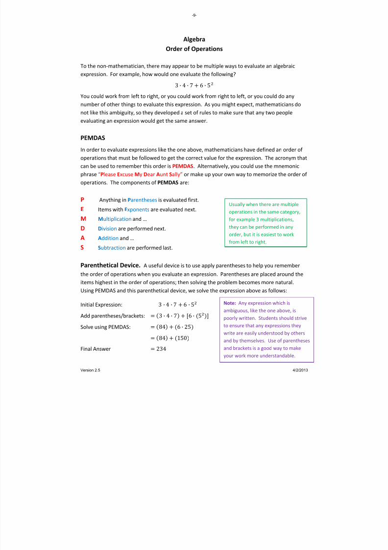
Parenthetical Device. A useful device is to use apply parentheses to help you remember
the order of operations when you evaluate an expression. Parentheses are placed around the
items highest in the order of operations; then solving the problem becomes more natural.
Using PEMDAS and this parenthe solve the expression above as follows: tical device, we
Initial Expression: 3 · 4 · 7 6 · 5
Add parentheses/brackets: 5
Note: Any expression which is
ambiguous, like the one above, is
poorly written. Students should strive
to ensure that any expressions they
write are easily understood by others
and by themselves. Use of parentheses
and brackets is a good way to make
your work more understandable.
3 · 4 · 7 6 ·
Solve using PEMDAS: 84 6 · 25
150 84
Final Answer 234
-9-
Version 2.5 4/2/2013
8/13/2019 AlgebraHandbook_very Helpful_ Print It
http://slidepdf.com/reader/full/algebrahandbookvery-helpful-print-it 10/178
Algebra Graphing with Coordinates
Graphs in two dimensions are very common in algebra and are one of the most common
algebra applications
in
real
life.
y
Coordinates Quadrant 2 Quadrant 1
The plane of points that can be graphed in 2 dimensions is
called the Rectangular Coordinate Plane or the Cartesian
Coordinate Plane (named after the French mathematician
and philosopher René Descartes).
x
Quadrant 3 Quadrant 4• Two axes are defined (usually called the x ‐ and y ‐axes).
• Each point
on
the
plane
has
an
x
value
and
a y
value,
written
as:
( x
-value,
y
-value)
• The point (0, 0) is called the origin, and is usually denoted with the letter “O”.
• The axes break the plane into 4 quadrants, as shown above. They begin with Quadrant 1
where x and y are both positive and increase numerically in a counter‐clockwise fashion.
Plotting Points on the Plane When plotting points,
• the x ‐value determines how far right (positive) or left (negative) of the origin the point is
plotted.
• The y ‐value determines how far up (positive) or down (negative) from the origin the point is
plotted.
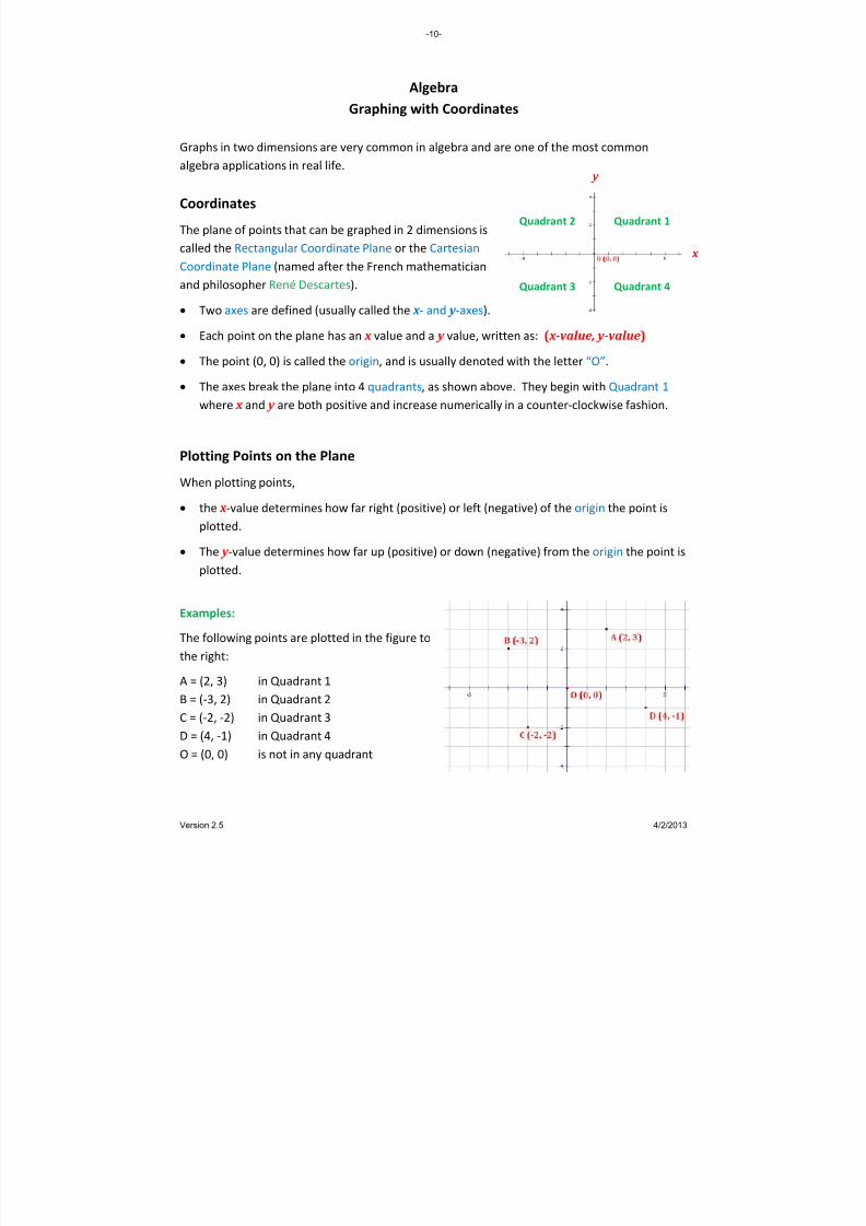
Examples: The following points are plotted in the figure to
the right:
A = (2, 3) in Quadrant 1
B = (‐3, 2) in Quadrant 2
C = (‐2, ‐2) in Quadrant 3
D = (4, ‐1) in Quadrant 4
O = (0, 0) is not in any quadrant
-10-
Version 2.5 4/2/2013

8/13/2019 AlgebraHandbook_very Helpful_ Print It
http://slidepdf.com/reader/full/algebrahandbookvery-helpful-print-it 11/178
Algebra Linear Patterns
Recognizing Linear Patterns The first step to recognizing a pattern is to arrange a set of numbers in a table. The table can
be either horizontal or vertical. Here, we consider the pattern in a horizontal format. More
advanced analysis generally uses the vertical format.
Consider this pattern:
x‐value 0 1 2 3 4 5
y‐value 6 9 12 15 18 21
To analyze
the
pattern,
we
calculate
differences
of
successive
values
in
the
table.
These
are
called first differences. If the first differences are constant, we can proceed to converting the
pattern into an equation. If not, we do not have a linear pattern. In this case, we may choose
to continue by calculating differences of the first differences, which are called second
differences, and so on until we get a pattern we can work with.
In the example above, we get a constant set of first differences, which tells us that the pattern
is indeed linear.
x‐value 0 1 2 3 4 5
y‐value
6
9
12
15
18
21
First Differences 3 3 3 3 3
Converting a Linear Pattern to an Equation
Creating an equation from the pattern is easy if you have
constant differences and a y‐value fo s case, r x = 0. In thi
• The equation takes the form , where
• “m” is
the
constant
difference
from
the
table,
and
• “b” is the y‐value when x = 0.
In the example above, this gives us the equation: .
Finally, it is a good idea to test your equation. For example, if 4, the above equation gives
3 · 4 6 18, which is the value in the table. So we can be pretty sure our equation is
correct.
Note: If the table does not have a
value for x=0, you can still obtain
the value of “b”. Simply extend the
table left or right until you have an
x‐value
of
0;
then
use
the
first
differences to calculate what the
corresponding y‐value would be.
This becomes your value of “b”.
-11-
Version 2.5 4/2/2013

8/13/2019 AlgebraHandbook_very Helpful_ Print It
http://slidepdf.com/reader/full/algebrahandbookvery-helpful-print-it 12/178
ADVANCED
n ∆
n ∆ ∆2
n ∆ ∆2
n ∆ ∆2
Identifying Number Patterns
In the
pattern
to
the
left,
notice
that
the
first
and
second
differences appear to be repeating the original sequence. When
this happens, the sequence may be recursive. This means that
each new term is based on the terms before it. In this case, the
equation is: y n = y n‐1 + y n‐2 , meaning that to get each new term,
you add the two terms before it.
‐3
‐1
1
3
5
7
17 29
26 211
When looking at patterns in numbers, is is often useful to take differences of the numbers you
are provided.
If
the
first
differences
are
not
constant,
take
differences
again.
23
5 25
10 27
2
2
2
2
2
37
52
7 24
11 48
19 816
35 1632
3 12
5 13
In the pattern to the left, notice that the first and second
differences are the same. You might also notice that these
differences are successive powers of 2. This is typical for an
exponential pattern. In this case, the equation is: y = 2 x
+ 3 .
When first differences are constant, the pattern represents a
linear equation. In this case, the equation is: y = 2x ‐ 5 . The
constant difference is the coefficient of x in the equation.
When second differences are constant, the pattern represents a
quadratic equation. In this case, the equation is: y = x 2 + 1 . The
constant difference, divided by 2, gives the coefficient of x2 in the
equation.
Algebra
8 25
13 38
21
When taking successive differences yields patterns that do not seem to level out, the pattern
may be
either
exponential
or
recursive.
21
67
-12-
Version 2.5 4/2/2013

8/13/2019 AlgebraHandbook_very Helpful_ Print It
http://slidepdf.com/reader/full/algebrahandbookvery-helpful-print-it 13/178
ADVANCED
n n
n ∆ ∆2
∆3
n ∆ ∆2
∆3
n ∆ ∆2
∆3
n ∆ ∆2
∆3
n ∆ ∆2
∆3
n ∆ ∆2
∆3
Completing Number Patterns
Algebra
The first step in completing a number pattern is to identify it. Then, work from the right to the left, filling in
the highest order differences first and working backwards (left) to complete the table. Below are two
examples.
‐17
6 1219 6
25 18
123
214
6
25
‐1
76 1219
214
37
25 1837
662 24
61 6123 30
91
662 24
61 6123
Consider in the examples the sequences of six
numbers which are provided to the student. You are
asked to find the ninth term of each sequence.
Example 1 Example 2
2
3
5
‐1
62 8
13
21
21
3 12 0
5 13 1
8
12 0
5 13 1
25 1
13 38
21
3
5
8 25 1
13 38 2
21
Step 1: Create a table of differences. Take successive
differences until you get a column of constant
differences (Example 1) or a column that appears to
repeat a previous column of differences (Example 2).
Step 2: In the last column of differences you created,
continue the constant differences (Example 1) or the
repeated differences
(Example
2)
down
the
table.
Create as many entries as you will need to solve the
problem. For example, if you are given 6 terms and
asked to find the 9th term, you will need 3 (= 9 ‐ 6)
additional entries in the last column.
‐1 27
24 8
6
2
13
6
3091 6
2146
6
3
261
16 12 3 1
19 6 2
Step 3: Work backwards (from right to left), filling in
each column by adding the differences in the column
to the right.
169 6 21
123 30 13 391
025 18 5 137 6 3 1
62
36 21 5127 6 13
8 2214
6 5 1
Column n: 214 + 127 = 341; 341 + 169 = 510; 510 + 217 = 727
The final answers to the examples are the ninth items in each sequence, the items in bold red.
In the example to the left, the calculations are
performed in the following order:
Column ∆2: 30 + 6 = 36; 36 + 6 = 42; 42 + 6 = 48
Column ∆: 91 + 36 = 127; 127 + 42 = 169; 169 + 48 = 217 5510 48 55 13
217 34727 89
341 42 34 8
-13-
Version 2.5 4/2/2013
8/13/2019 AlgebraHandbook_very Helpful_ Print It
http://slidepdf.com/reader/full/algebrahandbookvery-helpful-print-it 14/178
Algebra Basic Number Sets
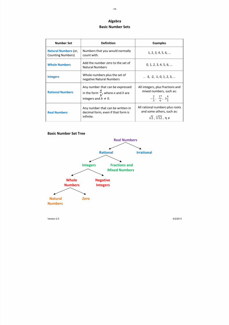
Number Set Definition Examples Natural Numbers (or, Counting Numbers) Numbers that you would normally
count with. 1, 2, 3, 4, 5, 6, …
Whole Numbers Add the number zero to the set of
Natural Numbers 0, 1, 2, 3, 4, 5, 6, …
Integers Whole numbers plus the set of
negative Natural Numbers … ‐3, ‐2, ‐1, 0, 1, 2, 3, …
Rational Numbers Any number that can be expressed
in the form
, where a and b are
integers and . 0 2
3
All integers, plus fractions and mixed numbers, such as:
,17
6, 3
4
5
Real Numbers Any number that can be written in
decimal form, even if that form is
infinite.
All rational numbers plus roots
and some others, such as:
√ 2 , √ 12
, π, e
Basic Number Set Tree Real Numbers
Rational Irrational Integers Fractions and
Mixed Numbers Whole Negative Numbers Integers
Natural Zero Numbers
-14-
Version 2.5 4/2/2013

8/13/2019 AlgebraHandbook_very Helpful_ Print It
http://slidepdf.com/reader/full/algebrahandbookvery-helpful-print-it 15/178
Algebra Operating with Real Numbers
Absolute Value The absolute value of something is the distance it is from zero. The easiest way to get the absolut a num o elimin e ign. A l values ositive or 0. e value of ber is t at its s bso ute are always p |5| 5 |3| 3 |0| 0
|1.5| 1.5 Adding and Subtracting Real Numbers
6 9 3 12 6 18
Adding Numbers with the Same Sign: • Add the numbers without regard
to sign. • Give the answer the same sign as
the original numbers. • Examples:
6 3 3 7 11 4
Adding Numbers with Different Signs: • Ignore the signs and subtract the
smaller number from the larger one. • Give the answer the sign of the number
with the greater absolute value. • Examples:
6 3 3 6 3 13 4 13 4 9
Subtracting Numbers: • Change the sign of the number or numbers being subtracted. • Add the resulting numbers. • Examples:
Multiplying and Dividing Real Numbers
6 18 · 3 112 3 4 4
8
the sign
• Give the answer a “+” sign.
Numbers with the Same Sign: • Multiply or divide numbers
without regard to . • Examples:
·6 3 18 12 3 4
Numbers with Different Signs: • Multiply or divide the numbers without
regard to sign. • Give the answer a “‐” sign. • Examples:
-15-
Version 2.5 4/2/2013
8/13/2019 AlgebraHandbook_very Helpful_ Print It
http://slidepdf.com/reader/full/algebrahandbookvery-helpful-print-it 16/178
Algebra Properties of Algebra
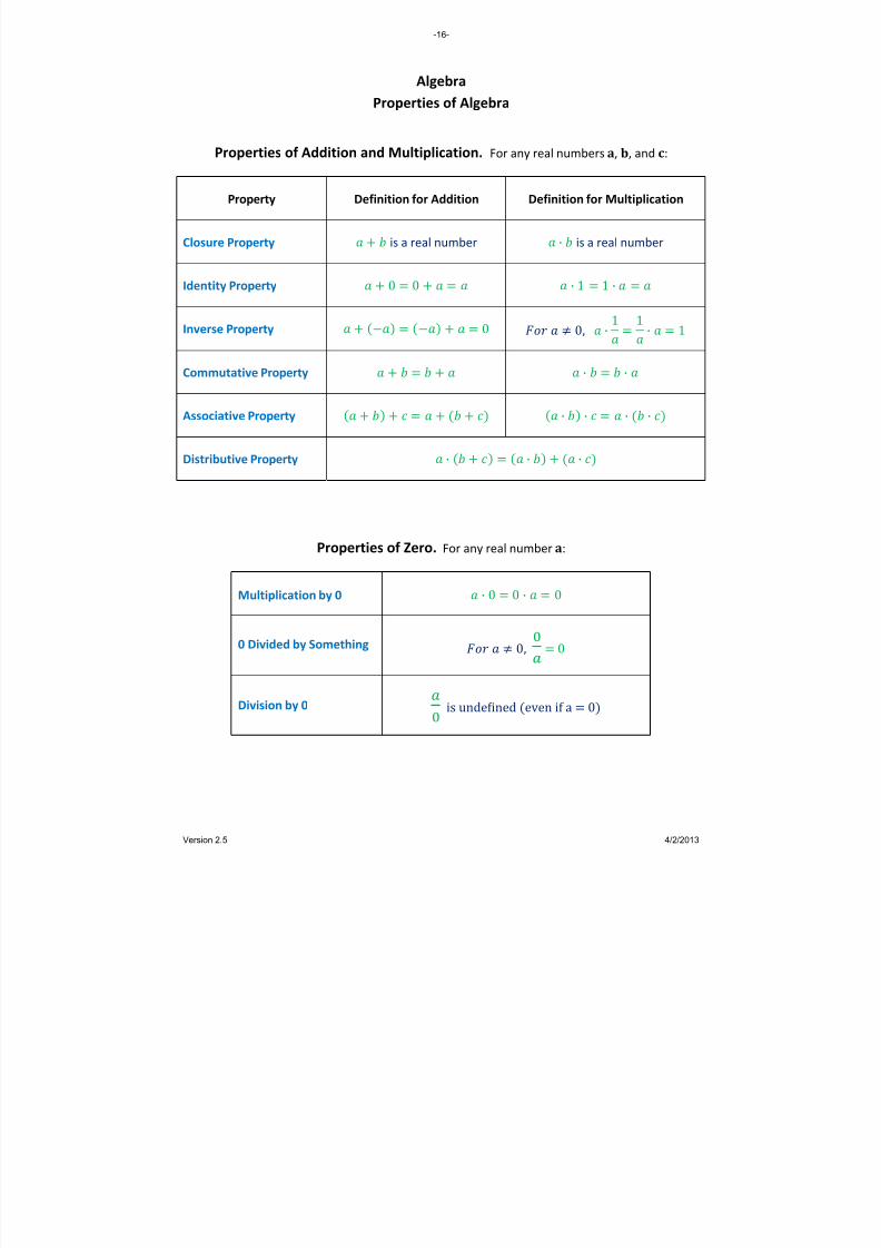
Properties of Addition and Multiplication. For any real numbers a, b, and c:
Property Definition for Addition Definition for Multiplication Closure Property is a real number · is a real number Identity Property 0 0 · 1 1 ·
Inverse Property 0
0, ·
1
1
· 1
Commutative Property · · Associative Property · · · · Distributive Property · · ·
Properties of Zero. For any real number a:
Multiplication by 0 · 0 0 · 0
0 Divided by Something 0, 0
Division by 0 is undeined even if a 0
-16-
Version 2.5 4/2/2013

8/13/2019 AlgebraHandbook_very Helpful_ Print It
http://slidepdf.com/reader/full/algebrahandbookvery-helpful-print-it 17/178
Algebra Properties of Algebra
Operational Properties of Equality. For any real numbers a, b, and c: Property Definition
Addition Property , Subtraction Property , Multiplication Property , · ·
Division Property 0,
Other Properties of Equality. For any real numbers a, b, and c:
Property Definition Reflexive Property Symmetric Property , Transitive Property , Substitution Property
If , then either can be substituted for theother in any equation (or inequality).
-17-
Version 2.5 4/2/2013
8/13/2019 AlgebraHandbook_very Helpful_ Print It
http://slidepdf.com/reader/full/algebrahandbookvery-helpful-print-it 18/178
Algebra
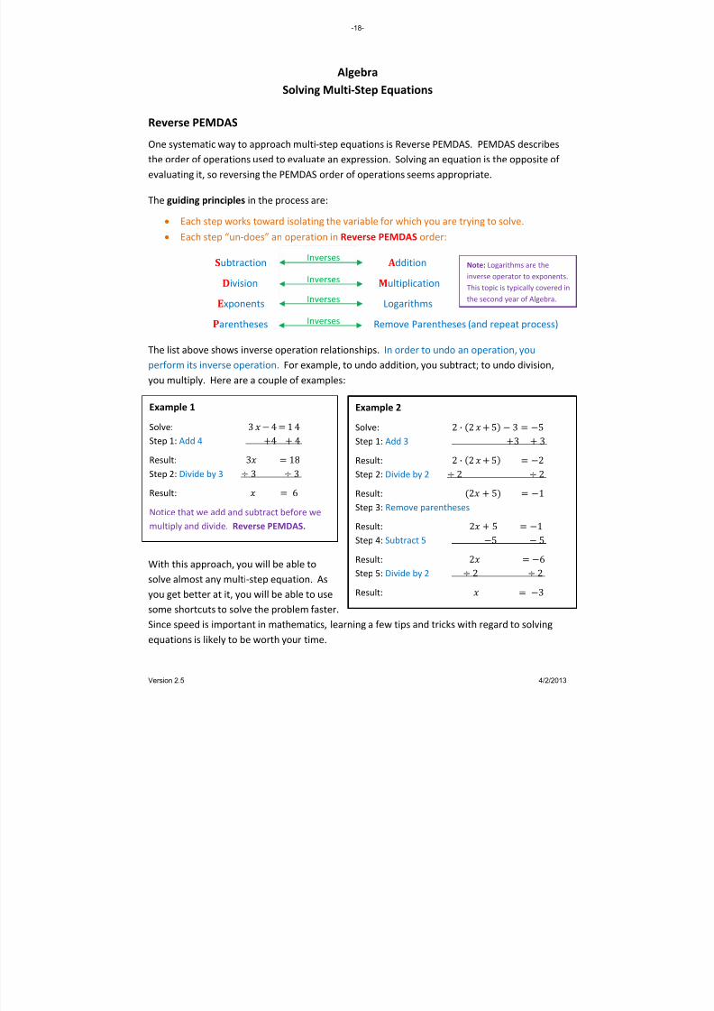
Solving Multi‐Step Equations
Reverse PEMDAS
One systematic way to approach multi‐step equations is Reverse PEMDAS. PEMDAS describes
the order of operations used to evaluate an expression. Solving an equation is the opposite of
evaluating it, so reversing the PEMDAS order of operations seems appropriate.
The guiding principles in the process are:
• Each step works toward isolating the variable for which you are trying to solve.
• Each step “un‐does” an operation in Reverse PEMDAS order:
Subtraction Addition
Division Multiplication
Exponents Logarithms
Parentheses Remove Parentheses (and repeat process)
Inverses
InversesNote: Logarithms are the
inverse operator
to
exponents.
This topic is typically covered in
the second year of Algebra. Inverses
The list above shows inverse operation relationships. In order to undo an operation, you
perform its inverse operation. For example, to undo addition, you subtract; to undo division,
you multiply. Here are a couple of examples:
Example 2
Solve: 2 · 2 5 53
Step 1: Add 3 3 3
Result: 2 · 2 5 2
Step 2: Divide by 2 2 2
Result: 2 5 1
Step 3: Remove parentheses
Result: 2 5 1
Step 4: Subtract 5 5 5
Result: 2 6
Step 5: Divide by 2 2 2
Result: 3
Inverses
Example 1
Solve: 3 4 1 4
Step 1: Add 4 4 4
Result: 3 18
Step 2: Divide by 3 3 3
Result: 6
Notice that we add and subtract before we
multiply and divide. Reverse PEMDAS.
With this approach, you will be able to
solve almost any multi‐step equation. As
you get better at it, you will be able to use
some shortcuts to solve the problem faster.
Since speed is important in mathematics, learning a few tips and tricks with regard to solving
equations is likely to be worth your time.
-18-
Version 2.5 4/2/2013

8/13/2019 AlgebraHandbook_very Helpful_ Print It
http://slidepdf.com/reader/full/algebrahandbookvery-helpful-print-it 19/178
Example 1
Solve:
8
Multiply by
:
·
·
Result:
· 8
12
Explanation: Since
is the reciprocal of
,
when we multiply them, we get 1, and
1 · . Using this approach, we can avoid
dividing by a fraction, which is more difficult.
Example 2
Solve:
2
Multiply by 4: · 4 · 4
Result:
2 · 4 8
Explanation: 4 is the reciprocal of
, so
when we multiply them, we get 1. Notice
the use of parentheses around the negative
number to make it clear we are multiplying
and
not
subtracting.
Example 3
Solve: 2 · 2 5 3 5
Step 1: Eliminate parentheses
Result: 4 1 0 3 5
Step
2:
Combine
constants
Result: 4 7 5
Step 3: Subtract 7 7 7
Result: 4 12
Step 4: Divide by 4 4 4
Result: 3
Algebra
Tips and Tricks in Solving Multi‐Step Equations
Fractional Coefficients
Fractions present a stumbling block to many students in solving multi‐step equations. When
stumbling blocks occur, it is a good time to develop a trick to help with the process. The trick
shown below involves using the reciprocal of a fractional coefficient as a multiplier in the
solution process. (Remember that a coefficient is a number that is multiplied by a variable.)
Another Approach to Parentheses
In the Reverse PEMDAS method, parentheses
are handled after all other operations.
Sometimes, it is easier to operate on the
parentheses first. In this way, you may be able
to re‐state the problem in an easier form before
solving it.
Example 3, at right, is another look at the
problem in Example 2 on the previous page.
Use whichever approach you find most to your
liking. They are both correct.
-19-
Version 2.5 4/2/2013
8/13/2019 AlgebraHandbook_very Helpful_ Print It
http://slidepdf.com/reader/full/algebrahandbookvery-helpful-print-it 20/178
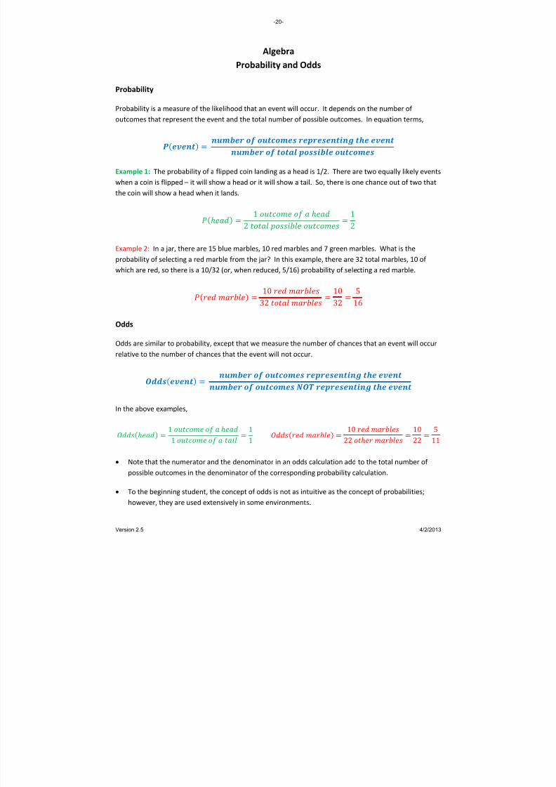
Algebra Probability and Odds
Probability Probability is a measure of the likelihood that an event will occur. It depends on the number of outcomes that represent the e on terms, vent and the total number of possible outcomes. In equati
Example 1: The probability of a flipped coin landing as a head is 1/2. There are two equally likely events when a coin is flipped – it will show a head or it will show a tail. So, there is one chance out of two that the coin will show a head when it lands.
1
2
1
2
Example 2: In a jar, there are 15 blue marbles, 10 red marbles and 7 green marbles. What is the probability of selecting a red marble from the jar? In this example, there are 32 total marbles, 10 of which are red, so there is a 10/32 (or, when red bility sele ting a red marble. uced, 5/16) proba of c
10
32
10
32
5
16
Odds Odds are similar to probability, except that we measure the number of chances that an event will occur relative to the number of chances that the event will not occur.
In the above examples,
1
1
1
1
10
22
10
22
5
11
• Note that the numerator and the denominator in an odds calculation add to the total number of possible outcomes in the denominator of the corresponding probability calculation.
• To the beginning student, the concept of odds is not as intuitive as the concept of probabilities; however, they are used extensively in some environments.
-20-
Version 2.5 4/2/2013
8/13/2019 AlgebraHandbook_very Helpful_ Print It
http://slidepdf.com/reader/full/algebrahandbookvery-helpful-print-it 21/178
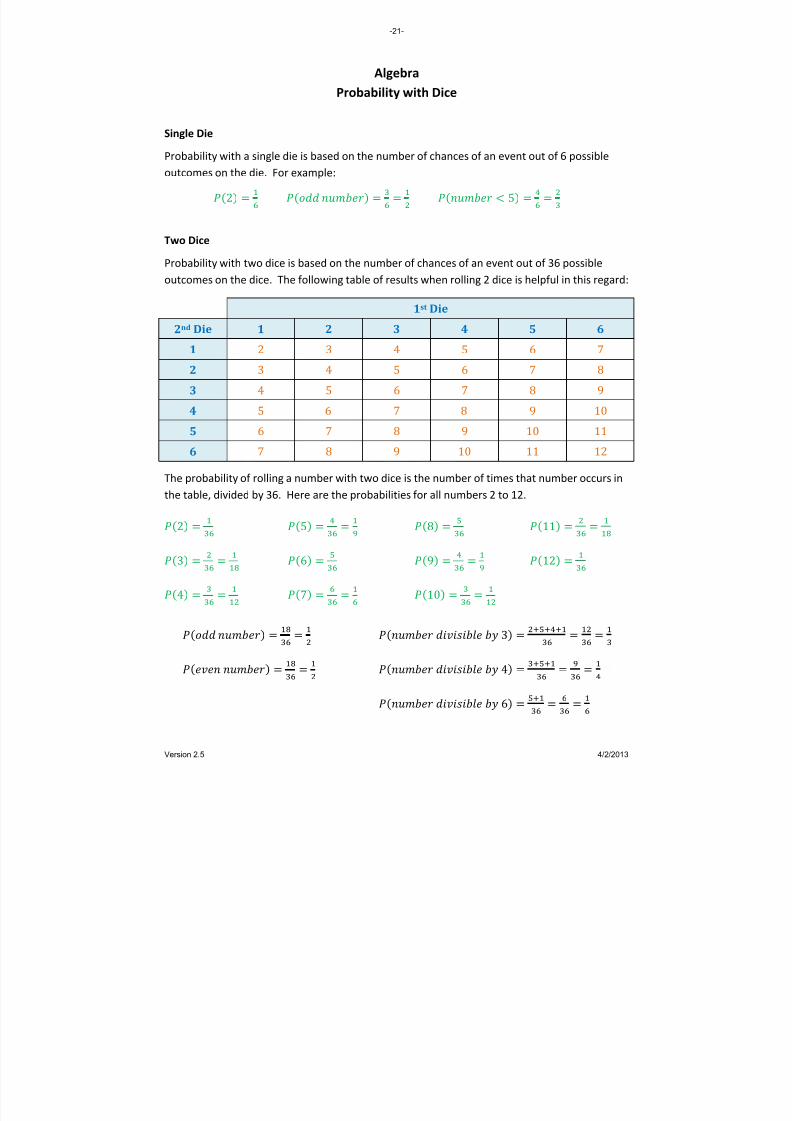
Algebra Probability with Dice
Single Die Probability with a single die is based on the number of chances of an event out of 6 possible outcomes on the die. For example:
2
5
Two Dice Probability with two dice is based on the number of chances of an event out of 36 possible outcomes on the dice. The following table of results when rolling 2 dice is helpful in this regard:
1st Die 2nd Die 1 2 3 4 5 6
1 2 3 4 5 6 7
2 3 4 5 6 7 8
3 4 5 6 7 8 9
4 5 6 7 8 9 10
5 6 7 8 9 10 11
6 7 8 9 10 11 12
The probability of rolling a number with two dice is the number of times that number occurs in the table, divided by 36. Here are the probabilities for all numbers 2 to 12. 2
5
8
11
3
6
9
12
4
7
10
3
4
6
-21-
Version 2.5 4/2/2013

8/13/2019 AlgebraHandbook_very Helpful_ Print It
http://slidepdf.com/reader/full/algebrahandbookvery-helpful-print-it 22/178
Algebra Combinations
Single Category Combinations The number of combinations of items selected from a set, several at a time, can be calculated relatively easily using the following technique:
Technique: Create a ratio of two products. In the numerator, start with the number of total items in the set, and count down so the total number of items being multiplied is equal to the number of items being selected. In the denominator, start with the number of items being selected and count down to 1.
Example: How many combinations of 3 items can be selected from a set of 8 items? A nswer:
8 · 7 · 6
3 · 2 · 1
56
Example: How many combinations of 4 items can be selected from a set of 13 item : s? Answer
1 3 · 1 2 · 1 1 · 1 0
4 · 3 · 2 · 1
715
Example: How many combinations of 2 items can be selected from a set of 30 items? : Answer
3 0 · 2 9
2 · 1
435
Multiple Category
Combinations
When calculating the number of combinations that can be created by selecting items from several categories, the technique is simpler:
Technique: Multiply the numbers of items in each category to get the total number of possible combinations.
Example: How many different pizzas could be created if you have 3 kinds of dough, 4 kinds of cheese and 8 kinds of toppings? Answer:
3 · 4 · 8 96
Example: How many different outfits can be created if you have 5 pairs of pants, 8 shirts and 4 jackets? Answer:
5 · 8 · 4 1 6 0
Example: How many designs for a car can be created if you can choose from 12 exterior colors, 3 interior colors, 2 interior fabrics and 5 types of wheels? Answer:
1 2 · 3 · 2 · 5 3 6 0
-22-
Version 2.5 4/2/2013
8/13/2019 AlgebraHandbook_very Helpful_ Print It
http://slidepdf.com/reader/full/algebrahandbookvery-helpful-print-it 23/178
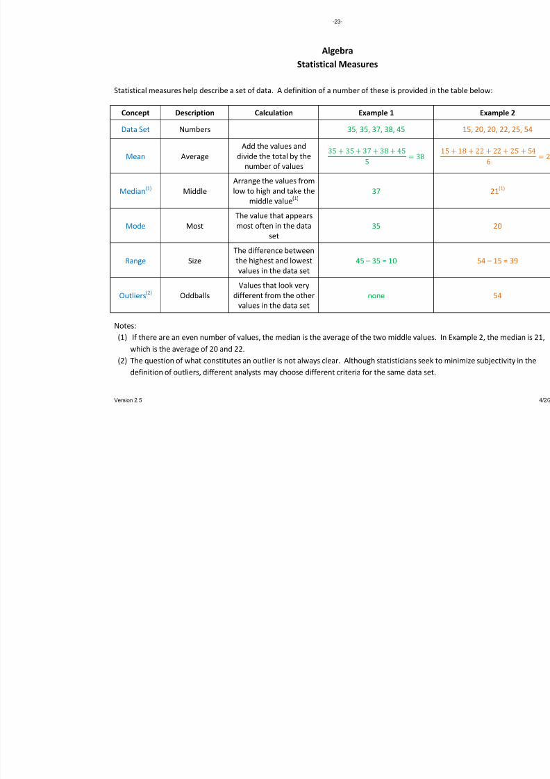
Algebra Statistical Measures
Statistical measures help describe a set of data. A definition of a number of these is provided in the tab
Concept Description Calculation Example 1 Data Set Numbers 35, 35, 37, 38, 45 Mean Average Add the values and
divide the total by the number of values
35
5
35 37 38 45 38 15 1
Median(1) Middle Arrange the values from
low to high and take the middle value
(1) 37
Mode Most The value that appears most often in the data
set 35
Range Size The difference between the highest and lowest values in the data set 45 – 35 = 10
Outliers(2) Oddballs Values that look very
different from the other values in the data set none
Notes: (1) If there are an even number of values, the median is the average of the two middle values. In Exa
which is the average of 20 and 22. (2) The question of what constitutes an outlier is not always clear. Although statisticians seek to mini
definition of outliers, different analysts may choose different criteria for the same data set.
-23-
Version 2.5

8/13/2019 AlgebraHandbook_very Helpful_ Print It
http://slidepdf.com/reader/full/algebrahandbookvery-helpful-print-it 24/178
Algebra
Introduction to Functions
Definitions
• A Relation is a relationship between variables, usually expressed as an equation.
• In a typical x - y equation, the Domain of a relation is the set of x ‐values for which y ‐
values can be calculated. For example, in the relation √ the domain is 0
because these are the values of x for which a square root can be taken.
• In a typical x - y equation, the Range of a relation is the set of y ‐values that result for all
values of the domain. For example, in the relation √ the range is 0 because
these are the values of y that result from all the values of x .
e doma• A Function is a relation in which each element in th in has only one
corresponding element in the range.
• A
One‐
to‐
One
Function
is
a
function
in
which
each
element
in
the
range
is
produced
by
only one element in the domain.
Function Tests in 2‐Dimensions
Vertical Line Test – If a vertical line passes through the graph of a relation in any two locations,
it is not a function. If it is not possible to construct a vertical line that passes through the graph
of a relation in two locations, it is a function.
Horizontal Line Test – If a horizontal line passes through the graph of a function in any two
locations, it is not a one‐to‐one function. If it is not possible to construct a horizontal line that
passes through
the
graph
of
a function
in
two
locations,
it
is
a one
‐to
‐one
function.
Examples:
Figure 1:
Not a function.
Fails vertical line test.
Figure 2:
Is a function, but not a one‐
to‐one function.
Passes vertical line test.
Fails horizontal line test.
Figure 3:
Is a one‐to‐one function.
Passes vertical line test.
Passes horizontal line test.
-24-
Version 2.5 4/2/2013

8/13/2019 AlgebraHandbook_very Helpful_ Print It
http://slidepdf.com/reader/full/algebrahandbookvery-helpful-print-it 25/178
Algebra Special Integer Functions
Greatest Integer Function Also called the Floor Function, this function gives the greatest integer less than or equal to a number. There are two common notations for this, as shown in the examples below. Notation and examples:
3.5 3 2.7 3 6 6 2.4 2 7.1 8 0 0
In the graph to the right, notice the solid dots on the left of the segments (indicating the points are included) and the open lines on the right of the segments (indicating the points are not included). Least Integer Function Also called the Ceiling Function, this function gives the least integer greater than or equal to a number. The common notation for this is shown in the examples below. Notation and examples:
3.5 4 2.7 2 6 6 In the graph to the right, notice the open dots on the left of the segments (indicating the points are not included) and the closed dots on the right of the segments (indicating the points are included). Nearest Integer Function Also called the Rounding Function, this function gives the nearest integer to a number (rounding to the even number when a value ends in .5). There is no clean notation for this, as shown in the examples below. Notation and examples:
3.5 4 2.7 3 6 6 In the graph to the right, notice the open dots on the left of the segments (indicating the points are not included) and the closed dots on the right of the segments (indicating the points are included).
-25-
Version 2.5 4/2/2013

8/13/2019 AlgebraHandbook_very Helpful_ Print It
http://slidepdf.com/reader/full/algebrahandbookvery-helpful-print-it 26/178
Algebra
Operations with Functions
Function Notation
Function notation replaces the variable y with a function name. The x in parentheses indicates
that x is the domain variable of the function. By convention, functions tend to use the letters f ,
g, and h as names of the function.
Operations with Functions
2
· 1
1, 1
Adding Functions
Subtracting Functions
Multiplying Functions · ·
Dividing Functions , 0
The domain of the combination
of
functions
is
the
intersection
of the domains of the two
individual functions. That is,
the combined function has a
value in its domain if and only if
the value is in the domain of
each individual function.
Examples:
Let: Then:
1 1
Note that in there is the requirement 1. This is because 10 in the
denominator would require dividing by 0, producing an undefined result.
Other Operations
Other operations of equa :lity also hold for functions, for example
·· · · ·
-26-
Version 2.5 4/2/2013

8/13/2019 AlgebraHandbook_very Helpful_ Print It
http://slidepdf.com/reader/full/algebrahandbookvery-helpful-print-it 27/178
Algebra
Composition of Functions
In a Composition of Functions, first one function is performed, and then the other. The
notation
for
composition
is,
for
example:
or .
In
both
of
these
notations,
the function g is performed first, and then the function f is performed on the result of g.
Always perform the function closest to the variable first.
Double Mapping
A composition can be thought of as a double mapping. First g maps from its domain to its
range. Then, f maps from the range of g to the range of f :
Example: Let
n a d 1
Then:
And:
The Words Method
In the
example,
• The function says square the argument .
• The function says add 1 to the argument .
Sometimes it is easier to think of the functions in
ather than in terms of an argument like x . words r
says “add 1 first, then square the result.” says “square first, then add 1 to the result.”
Using the
words
method,
f g
Calculate: o 2
f: square it 2 4
g: add 1 to it 4 1
Calculate: o 12
g: add 1 to it 12 1
f: square it
Range of g
Domain of f Domain of g Range of f
-27-
Version 2.5 4/2/2013

8/13/2019 AlgebraHandbook_very Helpful_ Print It
http://slidepdf.com/reader/full/algebrahandbookvery-helpful-print-it 28/178
Algebra
Inverses of Functions
In order for a function to have an inverse, it must be a one‐to‐one function. The requirement
for a function to be an inverse is:
The notation is used for the of Inverse Function .
Another way of saying this is that if , then for all in the domain of .
Deriving an Inverse Function
The following steps can be used to derive an inverse function. This process assumes that the
original function
is
expressed
in
terms
of
.
• Make sure the function is one‐to‐one. Otherwise it has no inverse. You can accomplish
this by graphing the function applying the vertical and horizontal line tests. and
• Substitute the variable y for .
• Exchange variables. That is, change all the x ’s to y ’s and all the y ’s to x ’s.
• Solve for the new y in terms of the new x .
• (Optional) Switch the e tion if you like. xpressions on each side of the equa
• Replace the variable y with the function notation . • Check your work.
Examples:
o 12 2 1 1
2
Derive the ver : in se of 2 Substitute for :
1
2 1
Exchange variables: 2 1
Add 1: 2 1 Divide by 2:
Switch sides:
Change Notation:
To check the result, note that:
o 3 6 3 13 2 6
Derive the ver : in se of
Substitute for :
2
2
Exchange variables: 2
Subtract 2: 2
Multiply by 3:
3 6
Switch sides: 3 6
Change Notation:
To check the result, note that:
-28-
Version 2.5 4/2/2013
8/13/2019 AlgebraHandbook_very Helpful_ Print It
http://slidepdf.com/reader/full/algebrahandbookvery-helpful-print-it 29/178
Algebra
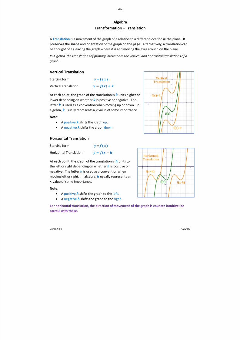
Transformation – Translation
A Translation is a movement of the graph of a relation to a different location in the plane. It
preserves the shape and orientation of the graph on the page. Alternatively, a translation can
be thought of as leaving the graph where it is and moving the axes around on the plane.
In Algebra, the translations of primary interest are the vertical and horizontal translations of a graph. Vertical Translation
Starting form:
Vertical Translation:
At each point, the graph of the translation is units higher or
lower depending on whether is positive or negative. The
letter is used as a convention when moving up or down. In
algebra, usually represents a y ‐value of some importance.
Note:
• A positive the graph up. shifts
• A negative shifts the graph down.
Horizontal Translation
Starting form:
Horizontal Translation:
At each point, the graph of the translation is units to
the left or right depending on whether is positive or
negative. The letter is used as a convention when
moving left or right. In algebra, usually represents an
x ‐value of some importance.
Note:
• A positive the graph to the left. shifts
• A negative shifts the graph to the right.
For horizontal translation, the direction of movement of the graph is counter‐intuitive; be
careful with these.
-29-
Version 2.5 4/2/2013
8/13/2019 AlgebraHandbook_very Helpful_ Print It
http://slidepdf.com/reader/full/algebrahandbookvery-helpful-print-it 30/178
Algebra
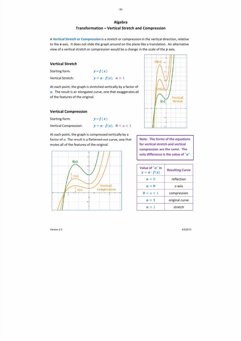
Transformation – Vertical Stretch and Compression
A Vertical Stretch or Compression is a stretch or compression in the vertical direction, relative
to the
x ‐axis. It does not slide the graph around on the plane like a translation. An alternative
view of a vertical stretch or compression would be a change in the scale of the y ‐axis.
Vertical Stretch
Starting form:
Vertical Stretch: · , 1
At each point, the graph is stretched vertically by a factor of
.
The result
is
an
elongated
curve,
one
that
exaggerates
all
of the features of the original.
Vertical Compression
Starting form:
Vertical Compression: · , 1
At each point, the graph is compressed vertically by a
factor of
. The
result
is
a flattened
‐out
curve,
one
that
mutes all of the features of the original.
Note:
The forms
of
the
equations
for vertical stretch and vertical
compression are the same. The
only difference is the value of "".
Value of "" in
·
Resulting Curve
0 reflection
x
‐axis
1 compression
original curve
1 stretch
-30-
Version 2.5 4/2/2013

8/13/2019 AlgebraHandbook_very Helpful_ Print It
http://slidepdf.com/reader/full/algebrahandbookvery-helpful-print-it 31/178
Algebra
Transformation – Horizontal Stretch and Compression
A Horizontal Stretch or Compression is a stretch or compression in the horizontal direction,
relative to the
y ‐axis. It does not slide the graph around on the plane like a translation. An
alternative view of a horizontal stretch or compression would be a change in the scale of the x ‐
axis.
Horizontal Stretch
Note: The forms of the equations
for the horizontal stretch and the
horizontal compression are the
same. The only difference is the
value of "".
Starting form:
Horizontal Stretch: ,
At each point, the graph is stretched horizontally
by a factor
of
.
The result
is
a widened
curve,
one
that exaggerates all of the features of the original.
Horizontal Compression
Starting form:
Horizontal Compression: ,
At each point, the graph is compressed horizontally by a
factor of . The result is a skinnier curve, one that mutes
all of the features of the original.
Value of "" in
Resulting Curve
0 reflection
horizontal line
1 stretch
original
curve
1 compression
Note: For horizontal stretch and compression, the change in the graph caused by the value
of “b” is counter‐intuitive; be careful with these.
-31-
Version 2.5 4/2/2013
8/13/2019 AlgebraHandbook_very Helpful_ Print It
http://slidepdf.com/reader/full/algebrahandbookvery-helpful-print-it 32/178
Algebra
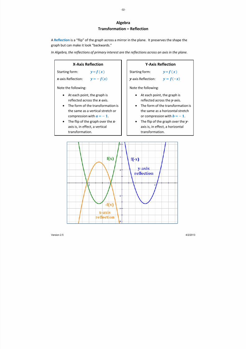
Transformation – Reflection
A Reflection is a “flip” of the graph across a mirror in the plane. It preserves the shape the
graph but can make it look “backwards.”
In Algebra, the reflections of primary interest are the reflections across an axis in the plane. X‐Axis Reflection
Starting form:
x ‐axis Reflection:
Note the following:
• At each
point,
the
graph
is
reflected across the x ‐axis.
• The form of the transformation is
the same as a vertical stretch or
compression with .
• The flip of the graph over the x ‐
axis is, in effect, a vertical
transformation.
Y‐Axis Reflection
Starting form:
y ‐axis Reflection:
Note the following:
• At each
point,
the
graph
is
reflected across the y ‐axis.
• The form of the transformation is
the same as a horizontal stretch
or compression with .
• The flip of the graph over the y ‐
axis is, in effect, a horizontal
transformation.
-32-
Version 2.5 4/2/2013
8/13/2019 AlgebraHandbook_very Helpful_ Print It
http://slidepdf.com/reader/full/algebrahandbookvery-helpful-print-it 33/178
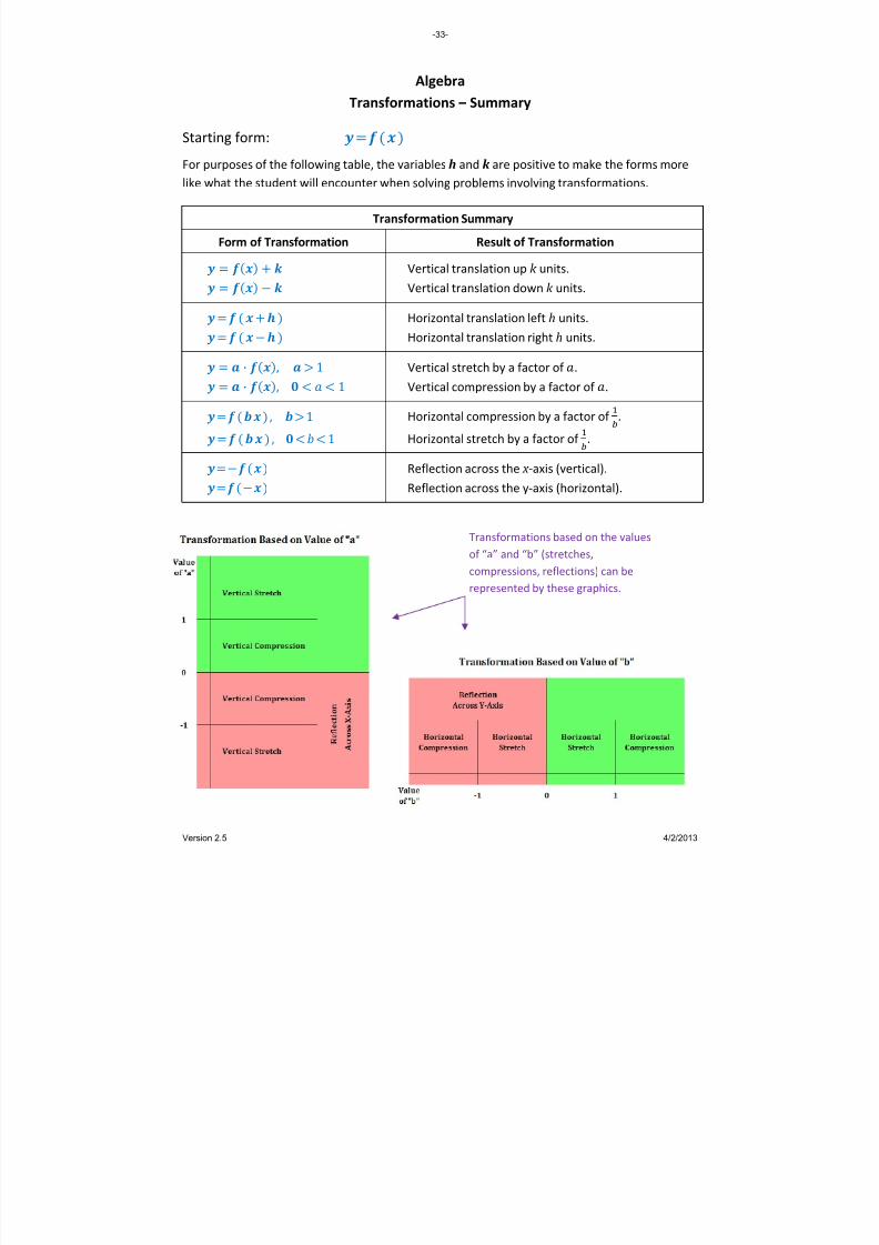
Algebra
Transform
Starting form:
ations – Summary
For purposes
of
the
following
table,
the
variables
h
and
k are
positive
to
make
the
forms
more
like what the student will encounter when solving problems involving transformations.
Transformation Summary
Form of Transformation Result of Transformation
Vertical translation up k units.
Vertical translation down k units.
Horizontal translation left h units.
Horizontal translation
right
h
its.
un
· , 1 Vertical stretch by a factor of .
· , 1 Vertical compression by a factor of .
, 1 Horizontal compression by a factor of .
, 1 Horizontal stretch by a factor of .
Reflection across the x ‐axis (vertical).
Reflection across the y‐axis (horizontal).
Transformations based on the values
of “a” and “b” (stretches,
compressions, reflections) can be
represented by these graphics.
-33-
Version 2.5 4/2/2013
8/13/2019 AlgebraHandbook_very Helpful_ Print It
http://slidepdf.com/reader/full/algebrahandbookvery-helpful-print-it 34/178
Algebra
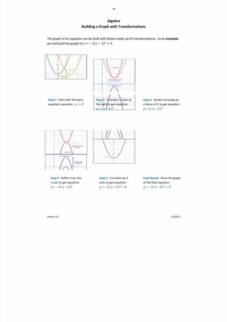
Building a Graph with Transformations
The graph of an equation can be built with blocks made up of transformations. As an example,
we will
build
the
graph
of
2 3 4.
Step 2: Translate 3 units to
the right to get equation:
Step 1: Start with the basic
quadratic equation:
Step 3: Stretch vertically by
a factor of 2 to get equation:
Step 4: Reflect over the
x ‐axis to get equation:
Step 5: Translate up 4
units to get equation:
Final Result: Show the graph
of the final equation:
-34-
Version 2.5 4/2/2013
8/13/2019 AlgebraHandbook_very Helpful_ Print It
http://slidepdf.com/reader/full/algebrahandbookvery-helpful-print-it 35/178
Algebra
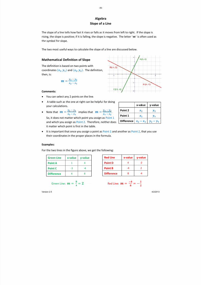
Slope of a Line
The slope of a line tells how fast it rises or falls as it moves from left to right. If the slope is
rising, the slope is positive; if it is falling, the slope is negative. The letter “m” is often used as
the symbol for slope.
The two most useful ways to calculate the slope of a line are discussed below.
Mathematical Definition of Slope
The definition is based on two points with
coordinates , and , . The definition,
then, is:
Comments:
• You can select any 2 points on the line.
• A table such as the one at right can be helpful for doing
your calculations.
• Note that
implies that
.
So, it does not matter which point you assign as Point 1
and which you assign as Point 2. Therefore, neither does
it matter which point is first in the table.
• It is important that once you assign a point as Point 1 and another as Point 2, that you use
their coordinates in the proper places in the formula.
x‐v lue a y‐value
Point 2
Point 1
Difference
Examples:
For the two lines in the figure above, we get the following:
Green Line: Red Line:
Green Line x‐value y‐value
Point A 1 4
Point C ‐3 ‐4
Difference 4 8
Red Line x‐value y‐value
Point D 4 ‐2
Point B ‐4 2
Difference 8 ‐4
-35-
Version 2.5 4/2/2013

8/13/2019 AlgebraHandbook_very Helpful_ Print It
http://slidepdf.com/reader/full/algebrahandbookvery-helpful-print-it 36/178
Algebra
Slope of a Line (cont’d)
Rise over Run
An equivalent method of calculating slope that is more
visual is the “Rise over Run” method. Under this
method, it helps to draw vertical and horizontal lines
that indicate the horizontal and vertical distances
between points on the line.
The slop cae can then be lculated as follows:
=
The rise of a line is how much it increases (positive) or decreases (negative) between two
points. The run is how far the line moves to the right (positive) or the left (negative) between
the same two points.
Comments:
• You can select any 2 points on the line.
• It is important to start at the same point in measuring both the rise and the run.
• A good convention is to always start with the point on the left and work your way to the
right; that way, the run (i.e., the denominator in the formula) is always positive. The only
exception to this is when the run is zero, in which case the slope is undefined.
• If the two points are clearly marked as integers on a graph, the rise and run may actually be
counted on the graph. This makes the process much simpler than using the formula for the
definition of slope. However, when counting, make sure you get the right sign for the slope
of the line, e.g., moving down as the line moves to the right is a negative slope.
Examples:
For the two lines in th o : e figure above, we get the foll wing
Green Line: Notice how similar the
calculations in the examples
are under the two methods
of calculating slopes. Red Line:
-36-
Version 2.5 4/2/2013

8/13/2019 AlgebraHandbook_very Helpful_ Print It
http://slidepdf.com/reader/full/algebrahandbookvery-helpful-print-it 37/178
Algebra
Slopes of Various Lines
line is vertical
When you look at a line, you
should notice the following
about its slope:
• Whether it is 0, positive, negative or undefined.
• If positive or negative, whether it is less than 1, about 1, or greater than 1.
The purpose of the graphs on
this page is to help you get a feel
for these
things.
This can help you check:
• Given a slope, whether you
drew the line correctly, or
• Given a line, whether you
calculated the slope
correctly.
2 45
line is steep and going down
3 12
line is steep and going up
1
line goes up at a 45⁰ angle 1
line goes down at a 45⁰ angle
317
line is shallow and going down
211
line is shallow and going up
0
line is horizontal
-37-
Version 2.5 4/2/2013

8/13/2019 AlgebraHandbook_very Helpful_ Print It
http://slidepdf.com/reader/full/algebrahandbookvery-helpful-print-it 38/178
Algebra
Various Forms of a Line
There are three forms of a linear equation which are most useful to the Algebra student, each
of which can be converted into the other two through algebraic manipulation. The ability to
move between forms is a very useful skill in Algebra, and should be practiced by the student.
Standard Form
Standa mples rd Form Exa
3 2 6
2 7 1 4
The Stan r o a linear equation is: da d Form f
where A, B, and C are real numbers and A and B are not both zero.
Usually in this form, the convention is for A to be positive.
Why, you might ask, is this “Standard Form?” One reason is that this form is easily extended to
additional variables, whereas other forms are not. For example, in four variables, the Standard
Form would be: . Another reason is that this form easily lends itself
to analysis with matrices, which can be very useful in solving systems of equations.
Slope‐Intercept Form
Slope‐ ples Intercept Exam
3 6
34 1 4
The Slope‐Intercept Form of a linear equation is the one most
familiar ents. It is: to many stud
where m is the slope and b is the y‐intercept of the line (i.e., the
value at which the line crosses the y‐axis in a graph). m and b must also be real numbers.
Point‐Slope Form
The Point‐Slope Form of a linear equation is the one used least by
the student, but it can be very useful in certain circumstances. In
particular, as you might expect, it is useful if the student is asked for
the equation of a line and is given the line’s slope and the
coordin e. The form of the equation is:
P oint‐Slope Examples
3 2 4
7 5 23 ates of a point on the lin
where m is the slope and , is any point on the line. One strength of this form is that
equations formed using different points on the same line will be equivalent.
-38-
Version 2.5 4/2/2013
8/13/2019 AlgebraHandbook_very Helpful_ Print It
http://slidepdf.com/reader/full/algebrahandbookvery-helpful-print-it 39/178
Algebra
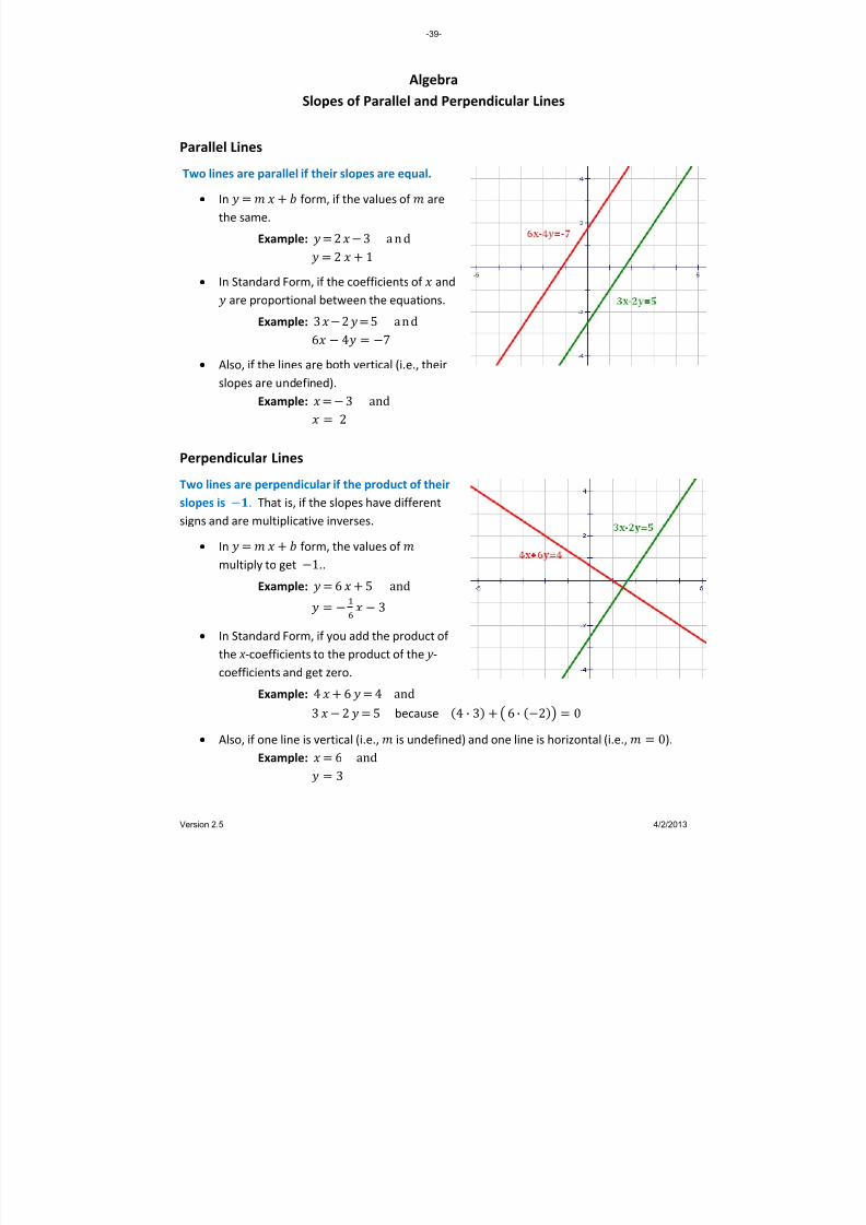
Slopes of Parallel and Perpendicular Lines
Parallel Lines
Two lines if their slopes are equal. are parallel
• In form, if the values of are
the same.
Example: 2 3 a n d 2 1
• In Standard Form, if the coefficients of and
are proportiona ions. l between the equat
Example:
3 2 5 a nd
4 6 7• Also, if the lines are both vertical (i.e., their
slopes are undefin de ).
Example: and 3 2
Perpendicular Lines
Two lines are perpendicular if the product of their
slopes is
. That is, if the slopes have different
signs and tive inverses. are multiplica
• In form, the values of
multiply to get 1..
Example: and 6 5
3
• In Standard Form, if you add the product of
the x ‐coefficients to the product of the y ‐
coefficients and get zero.
Example: and 4 6 4 3 2 5 because 4 · 3 6 · 2 0
• Also, if one line is is undefined) and one line is horizontal (i.e., 0). vertical (i.e.,
Example: and 6 3
-39-
Version 2.5 4/2/2013

8/13/2019 AlgebraHandbook_very Helpful_ Print It
http://slidepdf.com/reader/full/algebrahandbookvery-helpful-print-it 40/178
Algebra
Parallel, Perpendicular or Neither
The following flow chart can be used to determine whether a pair of lines are parallel, perpendicular, or neither.
yes
yes
no
no
Are the
slopes of the
two lines the
same?
First, put both lines in:
form.
Is the
product of
the two
slopes = ‐1?
Result: The lines are neither.
Result: The lines are parallel.
Result: The lines are
perpendicular.
-40-
Version 2.5 4/2/2013
8/13/2019 AlgebraHandbook_very Helpful_ Print It
http://slidepdf.com/reader/full/algebrahandbookvery-helpful-print-it 41/178
Algebra
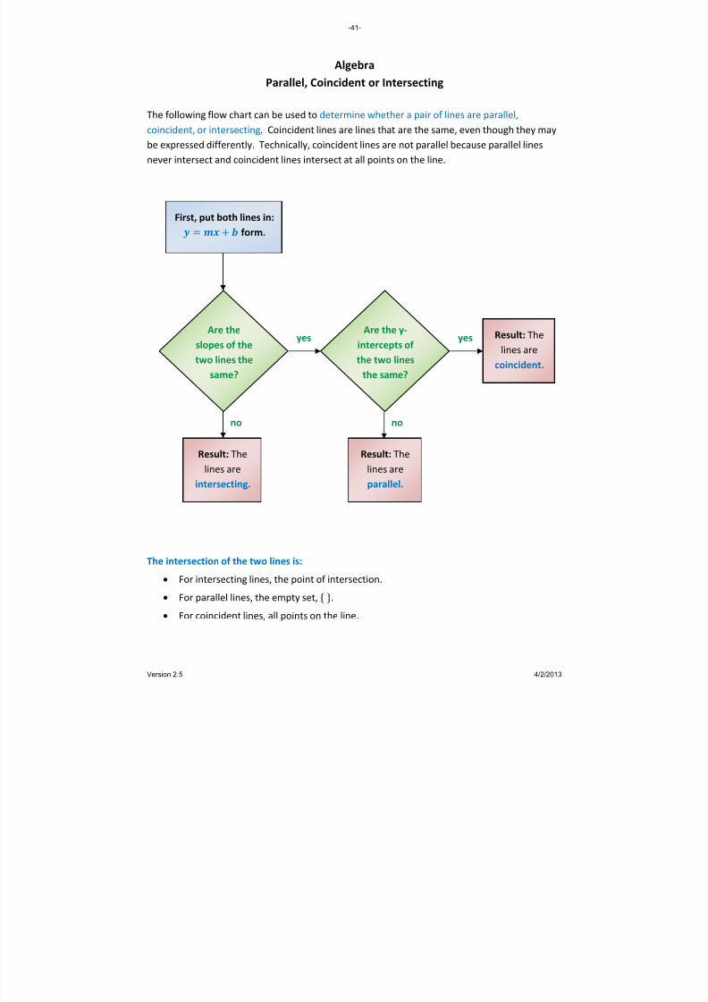
Parallel, Coincident or Intersecting
The following flow chart can be used to determine whether a pair of lines are parallel, coincident, or intersecting. Coincident lines are lines that are the same, even though they may be expressed differently. Technically, coincident lines are not parallel because parallel lines never intersect and coincident lines intersect at all points on the line.
The intersection of the two lines is:
• For intersecting lines, the point of intersection. • For parallel lines, the empty set, . • For coincident lines, all points on the line.
yes yes
no no
Are the
slopes of the
two lines the
same?
First, put both lines in:
form.
Are the y‐
intercepts of
the two lines
the same?
Result: The lines are
coincident.
Result: The lines are parallel.
Result: The lines are
intersecting.
-41-
Version 2.5 4/2/2013

8/13/2019 AlgebraHandbook_very Helpful_ Print It
http://slidepdf.com/reader/full/algebrahandbookvery-helpful-print-it 42/178
Algebra
Properties of Inequality
For any real numbers a, b, and c:
Property Definit on i
Addition
Property
,
,
Subtraction
Property
,
,
Multiplication
Property
For , 0
, · ·
, · ·
For , 0
, · ·
, · ·
Division
Property
For 0 ,
,
,
For 0 ,
,
,
Note: all properties which hold for “<” also hold for “≤”, and all properties which hold for “>”
also hold for “≥”.
There is nothing too surprising in these properties. The most important thing to be obtained
from them can be described as follows: When you multiply or divide an inequality by a
negative number, you must “flip” the sign. That is, “<” becomes “>”, “>” becomes “<”, etc.
In addition, it is useful to note that you can flip around an entire inequality as long as you keep
the “pointy” p the sign directed at the sam . Examples: art of e item
is the same as 4 4
3 2 is the same as 3 2
One way to remember this
is that when you flip around
an inequality, you must also
flip around the sign.
-42-
Version 2.5 4/2/2013

8/13/2019 AlgebraHandbook_very Helpful_ Print It
http://slidepdf.com/reader/full/algebrahandbookvery-helpful-print-it 43/178
Algebra
Graphs of Inequalities in One Dimension
Inequalities in one dimension are generally graphed on the number line. Alternatively, if it is
clear that the graph is one‐dimensional, the graphs can be shown in relation to a number line
but not specifically on it (examples of this are on the next page).
One‐Dimensional Graph Components
• The endpoint(s) – The endpoints for the ray or segment in the graph are shown as either
open or closed circles.
o If the point is included in the solution to the inequality (i.e., if the sign is ≤or ≥), the
circle is closed.
o If the point is not included in the solution to the inequality (i.e., if the sign is < or >),
the circle is open.
• The arrow – If all numbers in one direction of the number line are solutions to the
inequality, an arrow points in that direction.
o For < or ≤signs, the arrow points to the left ( ).
o For > or ≥signs, the arrow points to the right ( ).
• The line – in a simple inequality, a line is drawn from the endpoint to the arrow. If there are
two
endpoints,
a
line
is
drawn
from
one
to
the
other.
Examples:
-43-
Version 2.5 4/2/2013

8/13/2019 AlgebraHandbook_very Helpful_ Print It
http://slidepdf.com/reader/full/algebrahandbookvery-helpful-print-it 44/178
Algebra
Compound Inequalities in One Dimension
Compound inequalities are a set of inequalities that must all be true at the same time. Usually,
there are two inequalities, but more than two can also form a compound set. The principles
described below easily extend to cases where there are more than two inequalities.
Compound Inequalities with the Word “AND”
An exam n qualities with the would be: ple of compound i e word “AND”
12 2 or 1 These are the same conditions,
expressed in two different forms. (Simple Form) (Compound Form)
Graphically, “AND” inequalities exist at points where the graphs of the individual inequalities
overlap. This is the “intersection” of the graphs of the individual inequalities. Below are two
examples of graphs of compound inequalities using the word “AND.”
A typical “AND” example: The result is a
segment that contains the points that overlap
the graphs of the individual inequalities.
“AND” compound inequalities sometimes result
in the empty set. This happens when no
numbers meet both conditions at the same time.
Compound Inequalities with the Word “OR”
Graphically, “OR” inequalities exist at points where any of the original graphs have points. This
is the “union” of the graphs of the individual inequalities. Below are two examples of graphs of
compound inequalities using the word “OR.”
A typical “OR” example: The result is a pair of
rays extending in opposite directions, with a
gap in between.
“OR” compound inequalities sometimes result in
the set of all numbers. This happens when every
number meets at least one of the conditions.
-44-
Version 2.5 4/2/2013

8/13/2019 AlgebraHandbook_very Helpful_ Print It
http://slidepdf.com/reader/full/algebrahandbookvery-helpful-print-it 45/178
Algebra
Inequalities in Two Dimensions
Graphing an inequality in two dimensions involves the following steps:
• Graph the underlying equation. • Make the line solid or dotted based on whether the inequality contains an “=” sign.
o For inequalities with “<” or “>” the line is dotted. o For inequalities with “≤” or “≥” the line is solid.
• Determine whether the region containing the solution set is above the line or below the line.
o For inequalities with “>” or “≥” the shaded region is above the line. o For inequalities with “<” or “≤” the shaded region is below the line.
• Shade in the appropriate region. Example:
Graph the solution set of the following system of inequality: 1
Step 1: Graph the underlying equation.
Step 2: Determine whether the line id or dotted: should be sol
1 the > sign does not contain “=”, so the line is dotted
Step 3: Determine the region to be shaded based on the sign in the equation: 1 the > sign indicates shading above the line
The solution set is the shaded area.
-45-
Version 2.5 4/2/2013

8/13/2019 AlgebraHandbook_very Helpful_ Print It
http://slidepdf.com/reader/full/algebrahandbookvery-helpful-print-it 46/178
Algebra Graphs of Inequalities in Two Dimensions
Dashed Line
Below the Line
Dashed Line Above the Line
Solid Line
Below the Line
Solid Line Above the Line
-46-
Version 2.5 4/2/2013
8/13/2019 AlgebraHandbook_very Helpful_ Print It
http://slidepdf.com/reader/full/algebrahandbookvery-helpful-print-it 47/178
Algebra Absolute Value Functions
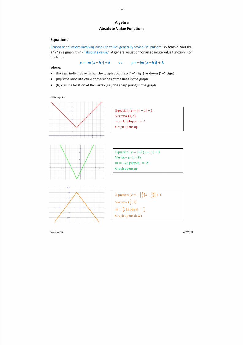
Equations Graphs of equations involving absolute values generally have a “V” pattern. Whenever you see a “V” in a graph, think “absolute value.” A general equation for an absolute value function is of the form:
|| || where, • the sign indicates whether the graph opens up (“” sign) or down (““ sign). • ||is the absolute value of the slopes of the lines in the graph. • (h, k) is the location of the vertex (i.e., the sharp point) in the graph. Examples:
Equation: | 1| 2Vertex = 1, 2 1; |slopes| 1Graph opens up
Equation: |21| 3Vertex = 1, 3 2; |slopes| 2Graph opens up
Equation:
3
Vertex = ,3
; |slopes|
Graph opens down
-47-
Version 2.5 4/2/2013

8/13/2019 AlgebraHandbook_very Helpful_ Print It
http://slidepdf.com/reader/full/algebrahandbookvery-helpful-print-it 48/178
Algebra
Absolute Value Functions (cont’d)
Inequalities
Since a positive number and a negative number can have the same absolute value, inequalities
involving absolute values must be broken into two separate equations. For example:
3 4 The first new equation is simply the original
equation without the absolute value sign.
| 3| 4
Note: the English is poor, but the math
is easier to remember with this trick!
Equation 1
Solve: 4 3
Step 1: Add 3 3 3
Result: 7
Equation 2
Solve: 3 4
Step 1: Add 3 3 3
Result: 1
3 4 Sign that determines
use of “AND” or “OR”
In the second new equation, two things
change: (1) the sign flips, and (2) the value on
the right side of the inequality changes its sign.
At this point the absolute value problem has converted into a pair of compound inequalities.
Next, we need to know whether to use “AND” or “OR” with the results. To decide which word
to
use,
look
at
the
sign
in
the
inequality;
then
…
• Use the word “AND” with “less thand” signs.
• Use the word “OR” with “greator” signs.
The solution to the above absolute value problem, then, is the same as the solution to the
followin t alities: g se of compound inequ
7 1 The solution set is all x in the range (‐1, 7)
Note: the solution set to this example is given in “range” notation. When using this notation,
• use parentheses ( ) whenever an endpoint is not included in the solution set, and
• use square brackets [ ] whenever an endpoint d in the solution set. is include
• Always use parentheses ( ) with infinity signs (∞ ∞).
The range: 6 2
Notation: 2, 6
The range: 2
Notation: ∞, 2
Examples:
-48-
Version 2.5 4/2/2013

8/13/2019 AlgebraHandbook_very Helpful_ Print It
http://slidepdf.com/reader/full/algebrahandbookvery-helpful-print-it 49/178
Algebra Systems of Equations
A system of equations is a set of 2 or more equations for which we wish to determine all
solutions which satisfy each equation. Generally, there will be the same number of equations
as variables and a single solution to each variable will be sought. However, sometimes there is
either no solution or there is an infinite number of solutions.
There are many methods available to solve a system of equations. We will show three of them
below.
Graphing a Solution In the simplest cases, a set of 2 equations in 2 unknowns can be solved using a graph. A single
equation in two unknowns is a line, so two equations give us 2 lines. The following situations
are possible with 2 lines:
• They will intersect. In this case, the point of intersection is the only solution.
• They will be the same line. In this case, all points on the line are solutions (note: this is
an infinite set).
• They will be parallel but not the same line. In this case, there are no solutions.
Examples
Solution Set: All points on the line.
Although the equations look
different, they actually
describe the same line.
Solution Set: The point of intersection
can be read off the graph;
the point (2,0).
Solution Set: The empty set;
these parallel lines
will never cross.
-49-
Version 2.5 4/2/2013

8/13/2019 AlgebraHandbook_very Helpful_ Print It
http://slidepdf.com/reader/full/algebrahandbookvery-helpful-print-it 50/178
Algebra Systems of Equations (cont’d)
Substitution Method
In the Substitution Method, we eliminate one of the variables by substituting into one of the
equations its equivalent in terms of the other variable. Then we solve for each variable in turn
and check the result. The steps s are illustrated in the example below. in this proces
Example: Solve for x and y if : and: 2 .
Step 1: Review the two equations. Look for a variable that can be substituted from one
equation into the other. In this example, we see a single “y” in the first equation; this is a prime
candidate for substitution.
We will substitute from the first equation for in the second equation.
Step 2: substitution. Perform the
becomes:
Step 3: l e uation for the single v e t. So ve the resulting q ariabl that is lef
Step 4: Substitute the known variable into one of the original equations to solve for the
remaini
After this step, the solution is tentatively identified as: , , meaning the point (3, -1).
ng variable.
Step 5: Check the result by substituting the solution into the equation not used in Step 4. If the
solution is correct, the result should be a true statement. If it is not, you have made a mistake
and should o r work carefully. check y u
Since this is a true mathematical
statement, the solution (3, -1) can
be accepted as correct.
-50-
Version 2.5 4/2/2013

8/13/2019 AlgebraHandbook_very Helpful_ Print It
http://slidepdf.com/reader/full/algebrahandbookvery-helpful-print-it 51/178
Algebra Systems of Equations (cont’d)
Elimination Method
In the Substitution Method, we manipulate one or both of the equations so that we can add
them and eliminate one of the variables. Then we solve for each variable in turn and check the
result. This is an outstanding method for systems of equations with “ugly” coefficients. The
steps in this process are illustrated in the example below. Note the flow of the solution on the
page.
Example: Solve for x and y if : and: 2 .
Step 6: Check the result by substituting
the solution into the equation not used in
Step 5. If the solution is correct, the
result should be a true statement. If it is
not, you have made a mistake and should
check your work.
2
Step 1: Re‐write the equations in
standard form.
Step 2: Multiply each equation by a value
selected so that, when the equations are added,
a variable will be eliminated.
(Multiply by 2)
(Multiply by ‐1) 2
Step 5: Substitute the result into
one of the original equations and
solve for the other variable.
U2
Step 3: Add the resulting equations.
Step 4: Solve for the variable.
Since this is a true mathematical statement, the
solution (3, -1) can be accepted as correct.
-51-
Version 2.5 4/2/2013
8/13/2019 AlgebraHandbook_very Helpful_ Print It
http://slidepdf.com/reader/full/algebrahandbookvery-helpful-print-it 52/178
Algebra Systems of Equations (cont’d)
Classification of Systems There
are
two
main
classifications
of
systems
of
equations:
Consistent
vs.
Inconsistent,
and
Dependent vs. Independent.
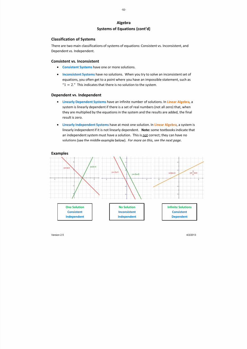
Consistent vs. Inconsistent • Consistent Systems have one or more solutions.
• Inconsistent Systems have no solutions. When you try to solve an inconsistent set of
equations, you often get to a point where you have an impossible statement, such as
“1 2.” This indicates that there is no solution to the system. Dependent vs. Independent
• Linearly Dependent Systems have an infinite number of solutions. In Linear Algebra, a
system is linearly dependent if there is a set of real numbers (not all zero) that, when
they are multiplied by the equations in the system and the results are added, the final
result is zero.
• Linearly Independent Systems have at most one solution. In Linear Algebra, a system is
linearly independent if it is not linearly dependent. Note: some textbooks indicate that
an independent system must have a solution. This is not correct; they can have no
solutions (see
the
middle
example
below).
For
more
on
this,
see
the
next
page.
Examples
One Solution Consistent
Independent No Solution Inconsistent Independent
Infinite Solutions Consistent Dependent
-52-
Version 2.5 4/2/2013

8/13/2019 AlgebraHandbook_very Helpful_ Print It
http://slidepdf.com/reader/full/algebrahandbookvery-helpful-print-it 53/178
ADVANCED Algebra
Linear Dependence
0
Linear dependence is a concept from Linear Algebra, and is very useful in determining if
solutions to complex systems of equations exist. Essentially, a system of functions is defined
to e of real numbers (not all zero) such that: be linearly depend nt if there is a set ,
… 0 or, in summation notation,
If there is no set of real numbers , such that the above equations are true, the system is said
to be linearly in e e n . d p n d e t
The expression
is called a linear combination of the functions
. The
importance of the concept of linear dependence lies in the recognition that a dependent
system is redundant, i.e., the system can be defined with fewer equations. It is useful to note
that a linearly dependent system of equations has a determinant of coefficients equal to 0.
Example: Consider the fo w ions: llo ing system of equat
Notice that: .
Therefore, the system is linearly
dependent.
Check th th coeffi nt atrix: ing e determinant of e cie m
3 2 11 1 21 0 5 1 2 11 2 0 3 11 2 5 3 21 1 15 07 51 0 .
It should be noted that the fact that D 0 is sufficient to prove linear dependence only if there
are no constant terms in the functions (e.g., if the problem involves vectors). If there are
constant terms, it is also necessary that these terms combine “properly.” There are additional
techniques to test this, such as the use of augmented matrices and Gauss‐Jordan Elimination.
Much of Linear Algebra concerns itself with sets of equations that are linearly independent. If
the determinant of the coefficient matrix is non‐zero, then the set of equations is linearly
independent.
-53-
Version 2.5 4/2/2013
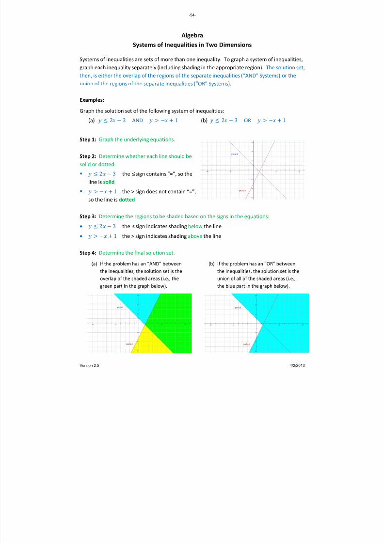
8/13/2019 AlgebraHandbook_very Helpful_ Print It
http://slidepdf.com/reader/full/algebrahandbookvery-helpful-print-it 54/178
Algebra Systems of Inequalities in Two Dimensions
Systems of inequalities are sets of more than one inequality. To graph a system of inequalities,
graph each inequality separately (including shading in the appropriate region). The solution set,
then, is either the overlap of the regions of the separate inequalities (“AND” Systems) or the
union of the regions of the separate inequalities (“OR” Systems).
Examples: Graph th t of the em of inequae solution se following syst lities:
(a) 2 3 AND 1 (b) 2 3 OR 1 Step 1: Graph the underlying equations.
Step 2: Determine whether each line should be
solid or dotted:
2 3 the ≤sign contains “=”, so the
line is solid
1 the > sign does not contain “=”,
so the line is dotted
Step ne the regions to be shaded based on the signs in the equations: 3: Determi
• the ≤sign indicates shading below the line 2 3 • 1 the > sign indicates shading above the line
Step 4: Determine the final solution set.
(a) If the problem has an “AND” between
the inequalities, the solution set is the
overlap of the shaded areas (i.e., the
green part in the graph below).
(b) If the problem has an “OR” between
the inequalities, the solution set is the
union of all of the shaded areas (i.e.,
the blue part in the graph below).
-54-
Version 2.5 4/2/2013

8/13/2019 AlgebraHandbook_very Helpful_ Print It
http://slidepdf.com/reader/full/algebrahandbookvery-helpful-print-it 55/178
Algebra Algebra Parametric Equations Parametric Equations
Parametric Equations in 2 dimensions are functions that express each of the two key variables
in terms of a one or more others. For exa
Parametric Equations in 2 dimensions are functions that express each of the two key variables
in terms of a one or more others. For example, mple,
Parametric equations are sometimes the most useful way to solve a problem. Parametric equations are sometimes the most useful way to solve a problem.
Pythagorean Triples Pythagorean Triples As a xample, the following parametric equations can be used to find Pythagorean Triples: As a xample, the following parametric equations can be used to find Pythagorean Triples: n e
Let
, be relatively prime integers and let
. Then, the following equations produce a set
of integer values that satisf
n e
Let
, be relatively prime integers and let
. Then, the following equations produce a set
of integer values that satisf y the Pythagorean Theorem:
y the Pythagorean Theorem:
Examples: Examples:
s s t t a a b b c c Pytha r nship Pytha r nship go ean Relatiogo ean Relatio
3 2 5 12 13 5 12 13
4 3 7 24 25 7 24 25
5 2 21 20 29 21 20 29 5 3 16 30 34 16 30 34
Creating a Standard Equation from Parametric Equations To create a standard equation from a set of
parametric equations in two dimensions, Example: Create a standard equation for the
parametr eic quations:
r in the , we get
Solving fo t : first equation
Substituting tion gives: into the second equa
ion
Cleaning this up, we seek: seek: we get the solut
• Solve one parametric equation for t .
• Substitute this value of t into the other
equation.
• Clean up the remaining expression as
necessary.
Note: any other method of solving
simultaneous equations can also be used for
this purpose.
-55-
Version 2.5 4/2/2013

8/13/2019 AlgebraHandbook_very Helpful_ Print It
http://slidepdf.com/reader/full/algebrahandbookvery-helpful-print-it 56/178
Algebra Exponent Formulas
Word Description
of Property
Math Description
of Property
Limitations
on variables
Product of Powers ·
Quotient of Powers
Power of a Power ·
Anything to the zero power is 1
Negative powers generate the reciprocal of what a positive
power generates
Power of a product ·
·
Power of a quotient
Converting a root to a power √
-56-
Version 2.5

8/13/2019 AlgebraHandbook_very Helpful_ Print It
http://slidepdf.com/reader/full/algebrahandbookvery-helpful-print-it 57/178
Algebra Scientific Notation
Format A
number
in
scientific
notation
has
two
parts:
• A number which is at least 1 and is less than 10 (i.e., it must have only one digit before
the decimal point). This number is called the coefficient.
• A power of 10 which is multiplied by the first number.
Here are a f regular scientific n ifew examples o
3
numbers expressed in
0.0 .
otat on.
132 .2 10
1,420,000 1.42 10
0034 3 4 10
1000 1 10
1 10
450 4.5 10
How many digits? How many zeroes? There are a couple of simple rules for converting from scientific notation to a regular number or
for converting from a regular number to scientific notation:
• If a regular number is less than 1, the exponent of 10 in scientific notation is negative.
The number of leading zeroes in the regular number is equal to the absolute value of
this exponent. In applying this rule, you must count the zero before the decimal point in
the regular number. Examples:
Original Number Action Conversion 0.00034 Count 4 zeroes 3.4 x 10
‐4
6.234 x 10‐8 Add 8 zeroes before the digits 0.000 000 062 34
• If the number is greater than 1, the number of digits after the first one in the regular
number is equal to the exponent of 10 in the scientific notation.
Original Number Action Conversion 4,800,000 Count 6 digits after the “4” 4.8 x 10⁶
9.6 x 10³
Add
3 digits
after
the
“9”
9,600
• As a general rule, multiplying by powers of 10 moves the decimal point one place for
each power of 10.
o Multiplying by positive powers of 10 moves the decimal to the right.
o Multiplying by negative powers of 10 moves the decimal to the left.
-57-
Version 2.5 4/2/2013

8/13/2019 AlgebraHandbook_very Helpful_ Print It
http://slidepdf.com/reader/full/algebrahandbookvery-helpful-print-it 58/178
Algebra Adding and Subtracting with Scientific Notation
When adding or subtracting numbers in scientific notation:
• Adjust the
numbers
so
they
have
the
same
power
of
10.
This
works
best
if you
adjust
the representation of the smaller number so that it has the same power of 10 as the
larger number. To do this:
o Call the difference between the exponents of 10 in the two numbers “n”.
o Raise the power of 10 of the smaller number by “n” , and
o Move the decimal point of the coefficient of the smaller number “n” places to
the left.
• Add the coefficients, keeping the power of 10 unchanged.
• If the result is not in scientific notation, adjust it so that it is.
o If the
coefficient
is
at
least
1 and
less
than
10,
the
answer
is
in
the
correct
form.
o If the coefficient is 10 or greater, increase the exponent of 10 by 1 and move the
decimal point of the coefficient one space to the left.
o If the coefficient is less than 1, decrease the exponent of 10 by 1 and move the
decimal point of the coefficient one space to the right.
Examples: 3.2 10
0.32 10
9.9 10 9 9. 0 10
10. 22 10
1.022 10
Explanation: A conversion of the smaller
number is required prior to adding because the
exponents of the two numbers are different.
After adding, the result is no longer in scientific
notation, so an extra step is needed to convert it
into the appropriate format.
6.1 10 6.1 10
2.3 10 2 .3 10
8. 4 10
1.2 10 1.20 10
4.5 10 0.45 10
0.75 10
7.5 10
Explanation: No conversion is necessary
because the exponents of the two numbers are
the same. After adding, the result is in scientific
notation, so no additional steps are required.
Explanation: A conversion of the smaller
number is required prior to subtracting because
the exponents of the two numbers are different.
After subtracting, the result is no longer in
scientific notation, so an extra step is needed to
convert it into the appropriate format.
-58-
Version 2.5 4/2/2013

8/13/2019 AlgebraHandbook_very Helpful_ Print It
http://slidepdf.com/reader/full/algebrahandbookvery-helpful-print-it 59/178
Algebra Multiplying and Dividing with Scientific Notation
When multiplying or dividing numbers in scientific notation:
• Multiply or divide the coefficients.
• Multiply or divide the powers of 10. Remember that this means adding or subtracting
the exponents while keeping the base of 10 unchanged.
o If you are multiplying, add the exponents of 10.
o If you are dividing, subtract the exponents of 10.
• If the result is not in scientific notation, adjust it so that it is.
o If the coefficient is at least 1 and less than 10, the answer is in the correct form.
o If the coefficient is 10 or greater, increase the exponent of 10 by 1 and move the
decimal point
of
the
coefficient
one
space
to
the
left.
o If the coefficient is less than 1, decrease the exponent of 10 by 1 and move the
decimal point of the coefficient one space to the right.
Examples: 4 10
· 5 10
Explanation: The coefficients are multiplied and
the exponents are added. After multiplying, the
result is no longer in scientific notation, so an
extra
step
is
needed
to
convert
it
into
the
appropriate format.
20 10
2.0 10
1.2 10
· 2.0 10
2. 4 10
Explanation: The coefficients are multiplied and
the exponents are added. After multiplying, the
result is in scientific notation, so no additional
steps are required.
3.3 10
Explanation: The coefficients are divided and
the exponents are subtracted. After dividing,
the result is no longer in scientific notation, so
an extra step is needed to convert it into the
appropriate format.
5.5 10
0.6 10
6.0 10
-59-
Version 2.5 4/2/2013
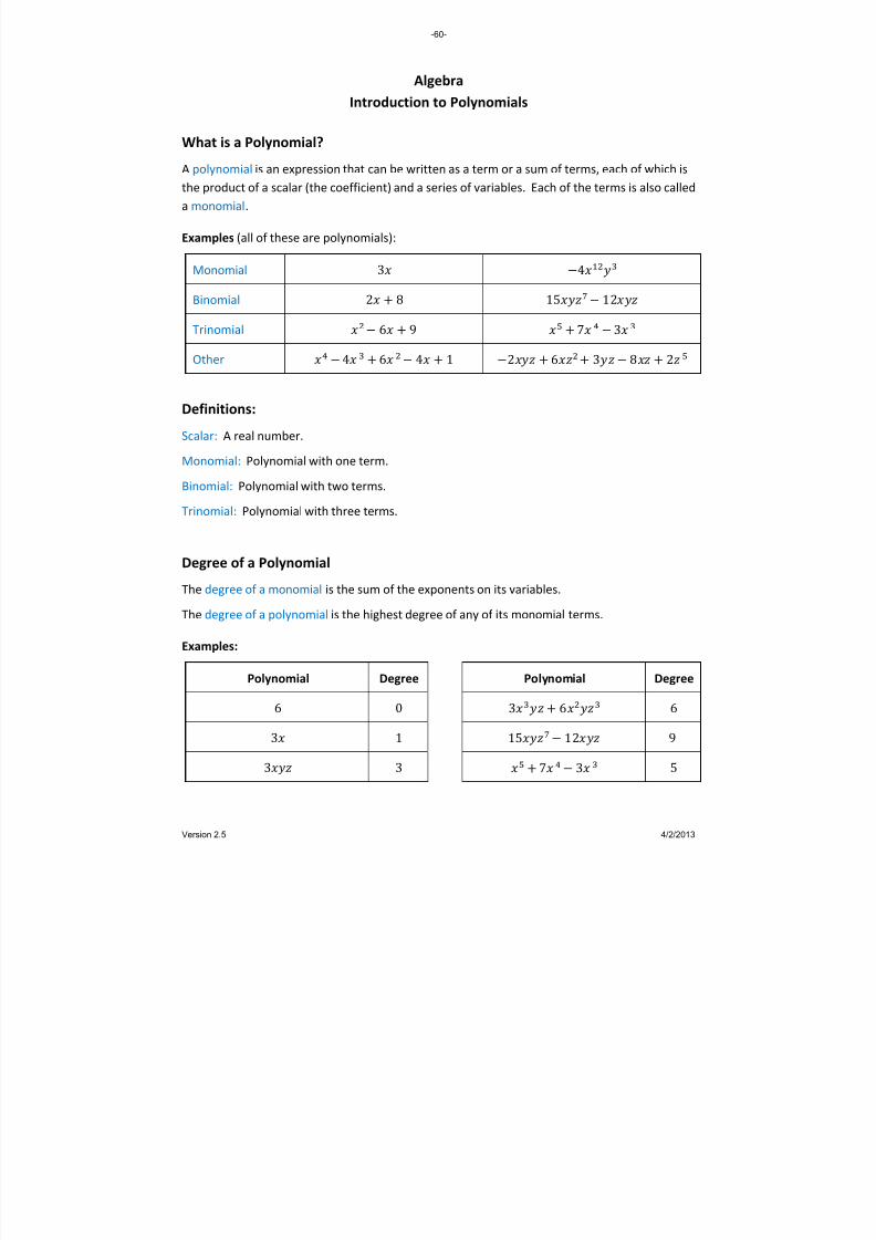
8/13/2019 AlgebraHandbook_very Helpful_ Print It
http://slidepdf.com/reader/full/algebrahandbookvery-helpful-print-it 60/178
Algebra Introduction to Polynomials
What is a Polynomial? A
polynomial
is
an
expression
that
can
be
written
as
a term
or
a sum
of
terms,
each
of
which
is
the product of a scalar (the coefficient) and a series of variables. Each of the terms is also called
a monomial.
Examples (all of these are polynomials):
Monomial 3 4
Binomial 2 8 1 5 12
Trinomial
6 9
7
3
Other 4 6 4 1 2 6 3 8 2
Definitions: Scalar: A real number.
Monomial: Polynomial with one term.
Binomial: Polynomial with two terms.
Trinomial: Polynomial with three terms.
Degree of a Polynomial The degree of a monomial is the sum of the exponents on its variables.
The degree of a polynomial is the highest degree of any of its monomial terms.
Examples: Polynomial Degree P aolynomi l Degree
6 0 3 6 6
3 1 15 12 9
3 3 7 3 5
-60-
Version 2.5 4/2/2013

8/13/2019 AlgebraHandbook_very Helpful_ Print It
http://slidepdf.com/reader/full/algebrahandbookvery-helpful-print-it 61/178
Algebra Adding and Subtracting Polynomials
Problems asking the studen written in linear form: t to add or subtract polynomials are often
Add: 3 2 4 2 4 6
The problem is much more easily solved if the problem is written in column form, with each
polynomial written in standard form.
Definitions Standard Form: A polynomial in standard form has its terms written from highest degree to
lowest degree from left to right.
Example: The standard form of 3 4 is 3 4
Like Terms:
Terms
with
the
same
variables
raised
to
the
same
powers.
Only
the
numerical
coefficients are different.
Example: 2, 6, and are like terms.
Addition and Subtraction Steps Step 1: Write each polynomial in standard form. Leave blank spaces for missing terms. For
example, if adding 3 2 4, leave space for the missing ‐term.
Step 2: If you are subtracting, change the sign of each term of the polynomial to be subtracted
and add
instead.
Adding
is
much
easier
than
subtracting.
Step 3: Place the polynomials in column form, being careful to line up like terms.
Step 4: Add the polynomials.
Examples: : 3 2 4 2 4 6
3 2 4
2 4 63 2 6 2
:
Solution: 3 2 4 2 4 6
3 2 4
2 4 63 2 2 10
Solution:
-61-
Version 2.5 4/2/2013

8/13/2019 AlgebraHandbook_very Helpful_ Print It
http://slidepdf.com/reader/full/algebrahandbookvery-helpful-print-it 62/178
Algebra Multiplying Binomials
The three methods shown below are equivalent. Use whichever one you like best. FOIL Method FOIL stands for First, Outside, Inside, Last. To multiply using the FOIL method, you make four
separate multiplicat a lts. ions and dd the resu
Example: Mult y · 3 4 ipl 2 3First:
2 3 · 3 9 12 4 6 8 6 12
The result is obtained by adding the results of
the 4 separate multiplications.
F O I L 2 · 3 6
Outside: 8 2 · 4 Inside: 93 · 3
Last: 3 · 4 12
Box Method The Box Method is pretty much the same as the FOIL method, except for the presentation. In
the box method, a 2x2 array of multiplications is created, the 4 multiplications are performed,
and the results are a dded.
Example: Multiply 2 3 · 3 4
Multiply 3x 2x 6 8
+3 9 12
2 3 · 3 9 12 4 6 8 6 12
The result is
obtained
by
adding
the
results
of
the 4 separate multiplications.
Stacked Polynomial Method 2 3 · 3 4
12 8 6 9
6 12
A third
method
is
to
multiply
the
binomials
like you would multiply 2‐digit numbers.
The name comes from how the two
polynomials are placed in a “stack” in
preparation for multiplication.
Example: Multiply 2 3 · 3 4
-62-
Version 2.5 4/2/2013

8/13/2019 AlgebraHandbook_very Helpful_ Print It
http://slidepdf.com/reader/full/algebrahandbookvery-helpful-print-it 63/178
Algebra Multiplying Polynomials
If the polynomials to be multiplied contain more than two terms (i.e., they are larger than
binomials), the FOIL Method will not work. Instead, either the Box Method or the Stacked
Polynomial Method should be used. Notice that each of these methods is essentially a way to
apply the distributive property of multiplication over addition.
The methods shown below are equivalent. Use whichever one you like best. Box Method The Box Method is the same for larger polynomials as it is for binomials, except the box is
bigger. An array of multiplications is created; the multiplications are performed; and like terms
are added.
Example: Multiply 2 2 3 ·2 3 4
Mu ply lti 2 3 4
4 6 8
4 6 8
6 9 12
4 2 2 3 ·2 3
24 3
64 4 6 6 8
9 8
Results:
Stacked Polynomial Method Results:
2 2 3
3 · 2 4
12 4 8 8 6 9 3 6
4 2 4 6
2 7 6 8 17 12
In the Stacked Polynomial Method, the
polynomials
are
multiplied
using
the
same
technique to multiply multi‐digit numbers
One helpful tip is to place the smaller
polynomial below the larger one in the
stack.
-63-
Version 2.5 4/2/2013

8/13/2019 AlgebraHandbook_very Helpful_ Print It
http://slidepdf.com/reader/full/algebrahandbookvery-helpful-print-it 64/178
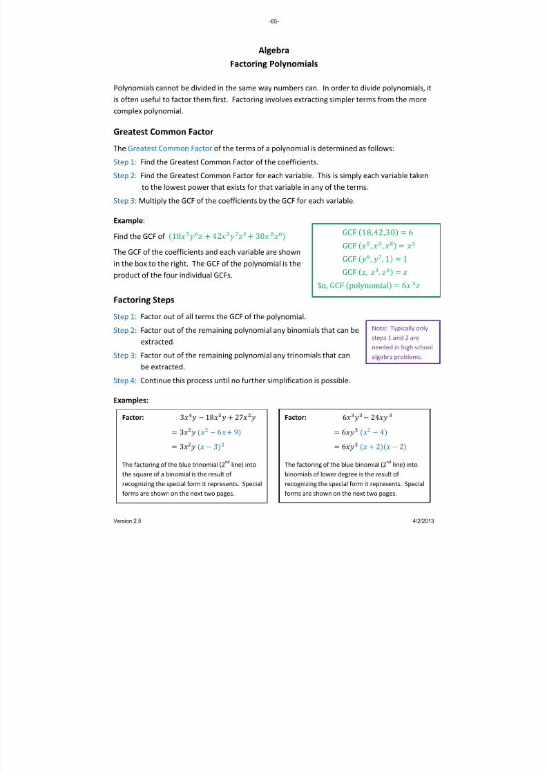
8/13/2019 AlgebraHandbook_very Helpful_ Print It
http://slidepdf.com/reader/full/algebrahandbookvery-helpful-print-it 65/178
Algebra Factoring Polynomials
Polynomials cannot be divided in the same way numbers can. In order to divide polynomials, it
is often useful to factor them first. Factoring involves extracting simpler terms from the more
complex polynomial.
Greatest Common Factor The Greatest Common Factor of the terms of a polynomial is determined as follows:
Step 1: Find the Greatest Common Factor of the coefficients.
Step 2: Find the Greatest Common Factor for each variable. This is simply each variable taken
to the lowest power that exists for that variable in any of the terms.
Step 3: Multiply the GCF of the coefficients by the GCF for each variable.
GCF 18,42,30 6
GCF , ,
GCF , , 1 1
GCF , ,
So, GCF polynomial 6
Example:
Find the GCF of 18 42 30
The GCF of the coefficients and each variable are shown
in the box to the right. The GCF of the polynomial is the
product of the four individual GCFs.
Factoring Steps Step
1:
Factor
out
of
all
terms
the
GCF
of
the
polynomial.
Note: Typically only
steps 1 and 2 are
needed in high school
algebra problems.
Step 2: Factor out of the remaining polynomial any binomials that can be
extracted.
Step 3: Factor out of the remaining polynomial any trinomials that can
be extracted.
Step 4: Continue this process until no further simplification is possible.
Examples: Factor:
3 18 27
9 3 6 3 3
The factoring of the blue trinomial (2nd
line) into
the square of a binomial is the result of
recognizing the special form it represents. Special
forms are shown on the next two pages.
Factor:
6 24
6 4 6 2 2
The factoring of the blue binomial (2nd
line) into
binomials of lower degree is the result of
recognizing the special form it represents. Special
forms are shown on the next two pages.
-65-
Version 2.5 4/2/2013

8/13/2019 AlgebraHandbook_very Helpful_ Print It
http://slidepdf.com/reader/full/algebrahandbookvery-helpful-print-it 66/178
Algebra Special Forms of Quadratic Functions
It is helpful to be able to recognize a couple special forms of quadratic functions. In particular,
if you can recognize perfect squares and differences of squares, your work will become easier
and more
accurate.
Perfect Squares Perfect squares are of the form:
Identification and Solution The following steps allow the student to identify and solve a trinomial that is a perfect square:
Step 1: Notice the first term of the trinomial is a square. Take its square root.
Step 2:
Notice
the
last
term
of
the
trinomial
is
a square.
Take
its
square
root.
Step 3: Multiply the results of the first 2 steps and double that product. If the result is the
middle term of the trinomial, the expression is a perfect square.
Step 4: The binomial in the solution is the sum or difference of the square roots calculated in
steps 1 and 2. The sign between the terms of the binomial is the sign of the middle
term of the trinomial.
–
Example:
√
Notice that the middle term is double the product
of the two square roots (
and
). This is a
telltale sign that the expression is a perfect square.
Identify the trinomial as a perfect square: • the of the first and last rms. They are 2 and 3. Take square roots te
• Test the middle term. Multiply the roots from the previous step, then double the result:
2 · 3 · 2 12. The result (with a “” sign in front) is the middle term of the
original trinomial. Therefore, the expression is a perfect square.
To express the trinomial as the square of a binomial: • The square roots of the first and last terms 2 and 3 make the binomial we seek. up
• We may choose the gn of the first term, so let’s c oose the “” sign. si h
• Having chosen the “” sign for the first term, the second term of the binomial takes the
sign of the middle term trinomial refore, the result is: of the original (“”). The
-66-
Version 2.5 4/2/2013

8/13/2019 AlgebraHandbook_very Helpful_ Print It
http://slidepdf.com/reader/full/algebrahandbookvery-helpful-print-it 67/178
Algebra Special Forms of Quadratic Functions
Differences of Squares Differences of squares are of the form: ·
These are much easier to recognize than the perfect squares because there is no middle term
to cons isider. Notice why there no middle term:
·
these two
terms cancel
Identification To see if an expression is a difference of squares, you must answer “yes” to four questions:
1. Are there only two terms?
2. Is there a “” sign between the two terms?
3. Is the first term a square? If so, take its square root.
4. Is the second term a square? If so, take its square root.
The solution is the product of a) the sum of the square roots in questions 3 and 4, and b) the
difference of the square roots in steps 3 and 4.
Note: A telltale sign of when an expression might be the difference of 2 squares is when the coefficients on the variables are squares: 1, 4, 9, 16, 25, 36, 49, 64, 81, etc. Examples:
(1) · (2) ·
(3) ·
(4)
·
· ADVANCED: Over the field of complex numbers, it is also possible to factor the sum of 2 squares:
This is not possible over the field of real numbers.
-67-
Version 2.5 4/2/2013

8/13/2019 AlgebraHandbook_very Helpful_ Print It
http://slidepdf.com/reader/full/algebrahandbookvery-helpful-print-it 68/178
coefficient of x
sign 1 sign 2 constant
Example: Factor
The numbers we seek are 4 and 7 because:
4 ∙ 7 28, and
∙
∙
∙
4 7 3
∙
7 ∙ 4 4 7 28
3 28
Algebra Factoring Trinomials – Simple Case Method
A common problem in Elementary Algebra is the factoring of a trinomial that is neither a perfect square nor a difference of squares. Consider the simple case where the coefficient of is 1. The general form for this case is:
∙
In order to simplify the illustration of factoring a polynomial where the coefficient of is 1, we will use the orange descriptors above for the components of the trinomial being factored. Simple Case Method Step 1: Set up parentheses for a pair of binomials. Put “ x ” in the
left hand position of each binomial. Step 2: Put sign 1 in the middle position in the left binomial. Step 3: Multiply sign 1 and sign 2 to get the sign for the right
binomial. Remember: ∙ ∙ ∙ ∙
Step 4: Find two numbers that: (a) Multiply to get the constant and ,
(b) Add to get the coefficient of Step 5: Place the numbers in the binomials so that their signs
match the
signs
from
Steps
2
and
3.
This
is
the
final
answer.
Step 6: Check your work by multiplying the two binomials to see if you get the original trinomial.
Fill in: ___ ∙ ___ ___ ___ ___ ___
-68-
Version 2.5 4/2/2013
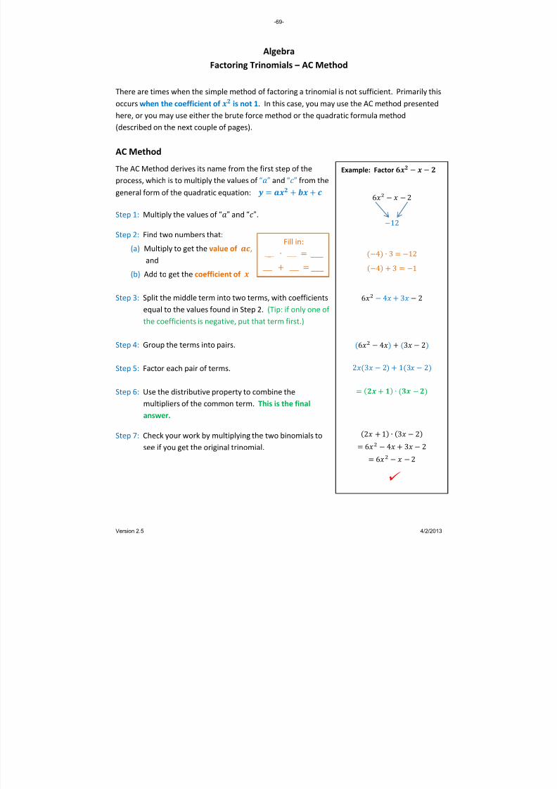
8/13/2019 AlgebraHandbook_very Helpful_ Print It
http://slidepdf.com/reader/full/algebrahandbookvery-helpful-print-it 69/178
Example: Factor
6 2 12
4 ∙ 3 12 4 3 1
6 4 3 2
6 4 3 2 23 2 13 2
∙
2 1 ∙ 3 2 6 4 3 2
6 2
Algebra Factoring Trinomials – AC Method
There are times when the simple method of factoring a trinomial is not sufficient. Primarily this occurs
when
the
coefficient
of
is
not
1.
In
this
case,
you
may
use
the
AC
method
presented
here, or you may use either the brute force method or the quadratic formula method (described on the next couple of pages). AC Method The AC Method derives its name from the first step of the process, which is to multiply the values of “” and “” from the general form of the quadratic equation: Step 1: Multiply the values of “” and “”. Step 2: Find two numbers that:
(a) Multiply to get the value of , and
(b) Add to get the coefficient of Step 3: Split the middle term into two terms, with coefficients
equal to the values found in Step 2. (Tip: if only one of the coefficients is negative, put that term first.)
Step 4: Group the terms into pairs. Step 5: Factor each pair of terms. Step 6: Use the distributive property to combine the
multipliers of the common term. This is the final answer.
Step 7: Check your work by multiplying the two binomials to see if you get the original trinomial.
Fill in: ___ ∙ ___ ___ ___ ___ ___
-69-
Version 2.5 4/2/2013

8/13/2019 AlgebraHandbook_very Helpful_ Print It
http://slidepdf.com/reader/full/algebrahandbookvery-helpful-print-it 70/178
Algebra Factoring Trinomials – Brute Force Method
When the coefficient of is not 1, the factoring process becomes more difficult. There are a
number of methods that can be used in this case.
If the question being asked is to find roots of the equation, and not to factor it, the student may
want to use the quadratic formula whenever the coefficient of is not 1. Even if you are
required to factor, and not just find roots, the quadratic formula may be a viable approach.
Brute Force Method
Example: Factor which equat
Combinations that produce a product
of 4 are:
1 and 4 or 2 and 2
Combinations that produce a product
of 3 are:
1 and 3 or 1 a d 3 n
14 3 14 33 13 1
4
4
2 12 3 12 2 3
14 3 4 3
14 3 4 3
34 1 4 11 3
34 1 4 11 3
2 12 3 4 4 3
42 12 3 4 3
4 4 3
This method is exactly what it sounds like. Multiple equations are possible and you must try
each of them until you find the one that works. Here are the steps to finding ions
are candidate solutions:
Step 1: Find all sets of whole numbers that multiply to
get the coefficient of the first term in the
trinomial. If the first term is positive, you need
only consider positive factors.
Step 2: Find all sets of whole numbers that multiply to
get the coefficient of the last term in the
trinomial. You must consider both positive and
negative factors.
Step 3: Create all possible products of binomials that
contain the whole numbers found in the first
two steps.
Step 4: Multiply the binomial pairs until you find one
that results in the trinomial you are trying to
factor.
Step 5: Identify the correct solution.
Notice the patterns in the candidate solutions in Step 4. Each pair of equations is identical except for
the sign of the middle term in the product. Therefore, you can cut your work in half by considering only
one of each pair until you see a middle term coefficient that has the right absolute value. If you have
everything right but the sign of the middle term, switch the signs in the binomials to obtain the correct
solution. Remember to check your work!
-70-
Version 2.5 4/2/2013

8/13/2019 AlgebraHandbook_very Helpful_ Print It
http://slidepdf.com/reader/full/algebrahandbookvery-helpful-print-it 71/178
Algebra Factoring Trinomials – Quadratic Formula Method
Quadratic Formula Method The Quadratic Formula is designed specifically to find roots of a second degree equation.
However, it can also be used as a back‐door method to factor equations of second degree. The
steps are:
Step 1: Apply the quadratic formula the roots of the equation. to determine
Step 2: Put each root into m: 0. the for
Step 3: Show the two binomials as a product. Note that these binomials may
contain fractions. We will eliminate the fractions, if p sible, in the next step. os
Step 4:
Multiply
the
binomials
in tep
3 by
the
coefficient
of
the
following
way:
S
(a) Break the coefficient of into its prime factors.
(b) Allocate the prime factors to the binomials in a way that eliminates the fractions.
Step 5: Check your work.
Example: Factor: Step
1:
√
√ or
Step 2: t ns containing roots are: The two equa io 0 and
0.
Step 3:
Step 4: The coefficient of in the original equation is 4, and 4 2 · 2. An inspection of the
binomials in Step 3 indicates we need to multiply each binomial by 2 in order to
eliminate the fractions:
2 · 2 3 and
2 · 2 1
So that: 4 4 3 · in factored form
Step 5: Check (using FOIL) 2 3 · 2 1 4 2 6 3 4 4 3 ,
which is the equation we were trying to factor.
-71-
Version 2.5 4/2/2013

8/13/2019 AlgebraHandbook_very Helpful_ Print It
http://slidepdf.com/reader/full/algebrahandbookvery-helpful-print-it 72/178
Algebra Algebra Solving Equations by Factoring Solving Equations by Factoring
There are a number of reasons to factor a polynomial in algebra; one of the most common
reasons is to find the zeroes of the polynomial. A “zero” is a domain value (e.g., x ‐value) for
which the polynomial generates a value of zero. Each zero is a solution of the polynomial.
There are a number of reasons to factor a polynomial in algebra; one of the most common
reasons is to find the zeroes of the polynomial. A “zero” is a domain value (e.g., x ‐value) for
which the polynomial generates a value of zero. Each zero is a solution of the polynomial.
In facto polynomial’s zeroes. Consider the following: In facto polynomial’s zeroes. Consider the following: red form, it is much easier to find a
2 4 8 3 is the factored form of a polynomial.
red form, it is much easier to find a
2 4 8 3 is the factored form of a polynomial.
If a number of items are multiplied together, the result is zero whenever any of the individual
items is zero. This is true for constants and for polynomials. Therefore, if any of the factors of
the polynomial has a value of zero, then the whole polynomial must be zero. We use this fact
to find zeroes of polynomials in factored form.
Example 1: Example 1: Find the zeroes of 2 4 8 3. Find the zeroes of 2 4 8 3.
Step 1: Set theStep 1: Set the equation equal to zero.
2 4 8 3 0
equation equal to zero.
2 4 8 3 0
Step 2: The wh is zero whenever any of its factors is zero. For the example, this
occurs
Step 2: The wh is zero whenever any of its factors is zero. For the example, this
occurs
ole equation
when:
or
ole equation
when:
or 2 0 ,
or
2 0 ,
or 4 0 ,
or
4 0 ,
or
The solution set, then, is:
ventionally, the x‐valu
2,4,8, ,3or, more con es are put
in numerical largest:
8 0 ,
or
8 0 ,
or 0 ,
3 0
0 ,
3 0
order from smallest to
4, 3, 2,, 8
The solution set contains the two
domain values that make the original
equation zero, namely:
1, 6 1, 6
Example 2: Example 2: Find
the
zeroes
of
Find
the
zeroes
of
7 6
0 7 6
0 7 6
6 1 0
7 6
6 1 0
0 0 0 0 6 1 6 1
6 1 6 1
Set Notation: We may list the set
of solutions to a problem by
placing the solutions in braces {},
separated by
commas.
-72-
Version 2.5 4/2/2013
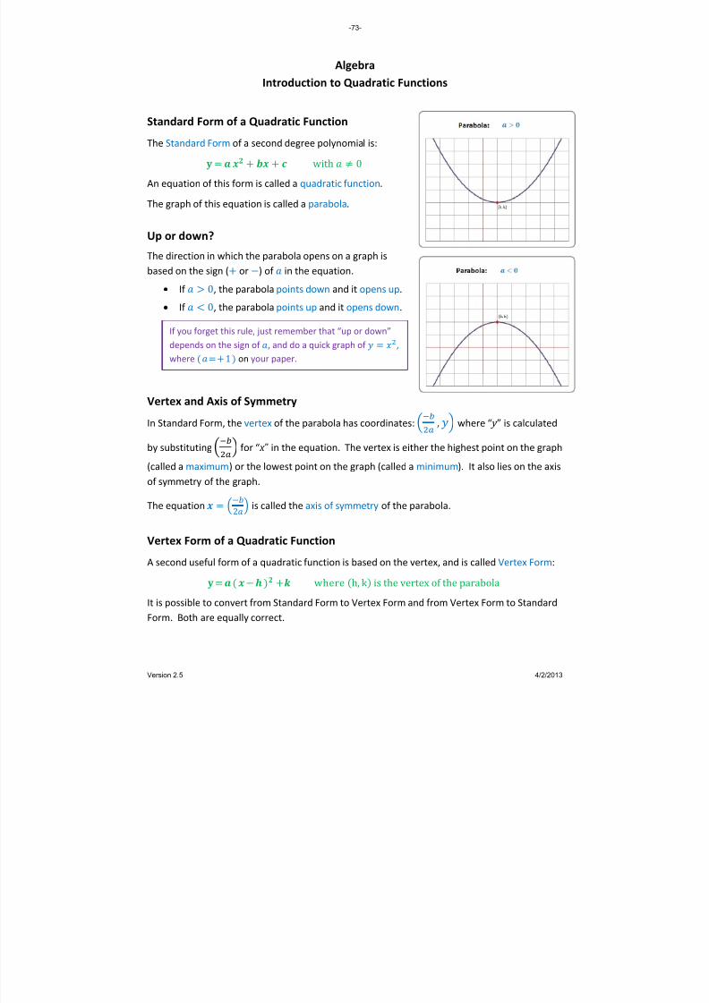
8/13/2019 AlgebraHandbook_very Helpful_ Print It
http://slidepdf.com/reader/full/algebrahandbookvery-helpful-print-it 73/178
Algebra Introduction to Quadratic Functions
Standard Form of a Quadratic Function The Standard a l is: Form of second degree polynomia
with 0
An equation of this form is called a quadratic function.
The graph of this equation is called a parabola.
Up or down? The direction in which the parabola opens on a graph is
based on n ( or ) of in the equation. the sig
• If the parabola points down and it opens up. 0,
• If 0, the parabola points up and it opens down.
If you forget this rule, just remember that “up or down”
depends on the sign of , and do a quick graph of ,
where 1 on your paper.
Vertex and
Axis
of
Symmetry
In Standard Form, the vertex of the parabola has coordinates:
, where “ y ” is calculated
by substituting for “ x ” in the equation. The vertex is either the highest point on the graph
(called a maximum) or the lowest point on the graph (called a minimum). It also lies on the axis
of symmetry o h. f the grap
The equation 2 is called the axis of symmetry of the parabola.
Vertex Form of a Quadratic Function A second usef ertex Form: ul form of a quadratic function is based on the vertex, and is called V
where h, k is the vertex of the parabolaIt is possible to convert from Standard Form to Vertex Form and from Vertex Form to Standard
Form. Both are equally correct.
-73-
Version 2.5 4/2/2013
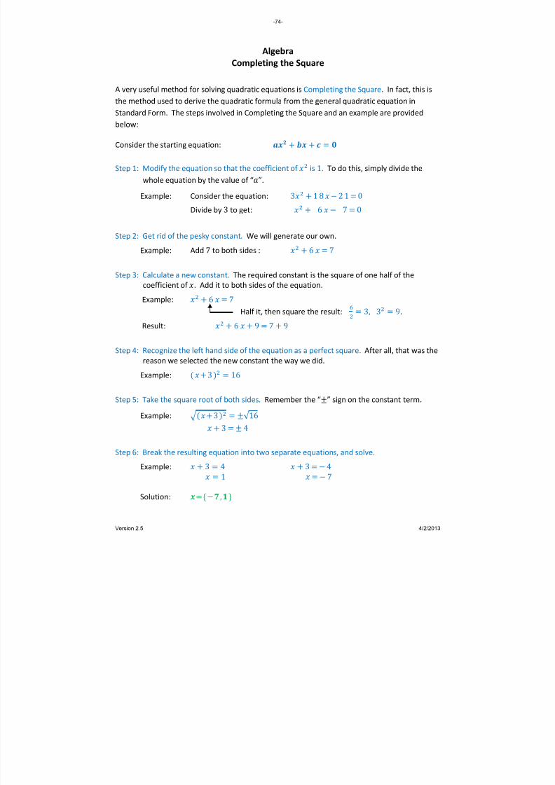
8/13/2019 AlgebraHandbook_very Helpful_ Print It
http://slidepdf.com/reader/full/algebrahandbookvery-helpful-print-it 74/178
Algebra Completing the Square
A very useful method for solving quadratic equations is Completing the Square. In fact, this is
the method used to derive the quadratic formula from the general quadratic equation in
Standard Form. The steps involved in Completing the Square and an example are provided
below:
Consider the starting equation:
Step 1: Modify the equation so that the coefficient of is 1. To do this, simply divide the
whole equation by the value of “”.
Example: Consider t e equation: 3 h 1 8 2 1 0
Divide by 3 to get: 6 7 0
Step 2: Get rid of the pesk constant. We will gene e y rat our own.
Example: Add 7 to both sides : 6 7
Step 3: Calculate a new constant. The required constant is the square of one half of the
coefficient of Add th sides of the equation. . it to bo
Example: 6 7
3,
3
9. uare the result:
Half it, then sq
Result: 6 9 7 9
Step 4: Recognize the left hand side of the equation as a perfect square. After all, that was the
reason we sele onstant the way we did. cted the new c
Example: 3 16
Step 5: Take the squa . Remember the “” sign on the constant term. re root of both sides
Example: 3 √ 16
3 4
Step 6: Break the resu ion into two separ s, and solve. lting equat ate equation
Example: 3 4 3 4
7 1
Solution: ,
-74-
Version 2.5 4/2/2013

8/13/2019 AlgebraHandbook_very Helpful_ Print It
http://slidepdf.com/reader/full/algebrahandbookvery-helpful-print-it 75/178
Algebra
Table of Powers and Roots Square Root Number Square Cube 4th Power
√ 1 1.000 1 1 1 1 1 1 1
√ 2 1.414 2 2 4 2 8 2 16
√ 3 1.732 3 3 9 3 27 3 81
√ 4 2.000 4 4 16 4 64 4 256
√ 5 2.236 5 5 25 5 125 5 625
√ 6 2.449 6 6 36 6 216 6 1,296
√ 7 2.646 7 7 49 7 343 7 2,401
√ 8 2.828 8 8 64 8 512 8 4,096
√ 9 3.000 9 9 81 9 729 9 6,561
√ 10 3.162 10 10 100 10 1,000 10 10,000
√ 11 3.317 11 11 121 11 1,331 11 14,641
√ 12 3.464 12 12 144 12 1,728 12 20,736
√ 13 3.606 13 13 169 13 2,197 13 28,561
√ 14 3.742 14 14
196 14
2,744 14
38,416√ 15 3.873 15 15 225 15 3,375 15 50,625
√ 16 4.000 16 16 256 16 4,096 16 65,536
√ 17 4.123 17 17 289 17 4.913 17 83,521
√ 18 4.243 18 18 324 18 5,832 18 104,976
√ 19 4.359 19 19 361 19 6,859 19 130,321
√ 20 4.472 20 20 400 20 8,000 20 160,000
√ 21 4.583 21 21 441 21 9,261 21 194,481
√ 22 4.690 22 22 484 22 10,648 22 234,256
√ 23 4.796 23 23 529 23 12,167 23 279841
√ 24 4.899 24 24 576 24 13,824 24 331,776
√ 25 5.000 25 25 625 25 15,625 25 390,625
-75-
Version 2.5 4/2/2013
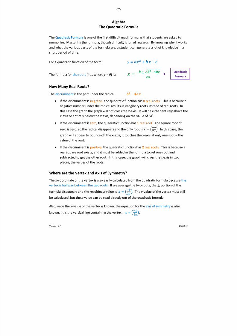
8/13/2019 AlgebraHandbook_very Helpful_ Print It
http://slidepdf.com/reader/full/algebrahandbookvery-helpful-print-it 76/178
Algebra The Quadratic Formula
The Quadratic Formula is one of the first difficult math formulas that students are asked to
memorize. Mastering the formula, though difficult, is full of rewards. By knowing why it works
and what the various parts of the formula are, a student can generate a lot of knowledge in a
short period of time.
For a quadratic function of the form:
The formula for the roots (i.e., where y = 0) is:
Quadratic Formula
How Many Real Roots? The discriminant is the part under the radical:
• If the discriminant is negative, the quadratic function has 0 real roots. This is because a
negative number under the radical results in imaginary roots instead of real roots. In
this case the graph the graph will not cross the x ‐axis. It will be either entirely above the
x ‐axis or entirely below the x ‐axis, depending on the value of “a”.
• If the discriminant is zero, the quadratic function has 1 real root. The square root of
zero is zero, so the radical disappears and the only root is 2. In this case, the
graph will appear to bounce off the x‐axis; it touches the x‐axis at only one spot – the
value of the root.
• If the discriminant is positive, the quadratic function has 2 real roots. This is because a
real square root exists, and it must be added in the formula to get one root and
subtracted to get the other root. In this case, the graph will cross the x ‐axis in two
places, the values of the roots.
Where are the Vertex and Axis of Symmetry? The
x ‐
coordinate
of
the
vertex
is
also
easily
calculated
from
the
quadratic
formula
because
the
vertex is halfway between the two roots. If we average the two roots, the portion of the
formula disappears and the resulting x ‐value is 2. The y ‐value of the vertex must still
be calculated, but the x ‐value can be read directly out of the quadratic formula.
Also, once the x ‐value of the vertex is known, the equation for the axis of symmetry is also
known. It is the vertical line containing the vertex: 2.
-76-
Version 2.5 4/2/2013

8/13/2019 AlgebraHandbook_very Helpful_ Print It
http://slidepdf.com/reader/full/algebrahandbookvery-helpful-print-it 77/178
Algebra Quadratic Inequalities in One Variable
Solve the inequality of the form: 0 Step 1: If "" is negative, multiply the whole inequality by "–1". This will make the problem
easier to work with t e the y. . Don’ forget to chang sign of the inequalit
Example: convert 3 9 6 0 to 3 9 6 0
Step 2: Factor out any scalars that divide into all of the terms of the inequality. This will also
make the problem easier to work with.
Example: factor 3 9 6 0 0 to 3 3 2 then divide by 3 to get: [ 3 2 0
Step 3: Solve the equation that corresponds to the inequality. The solutions of the equation
are the critical val f the inequalityues in the solution o .
Example: solve [ 3 2 0, which gives: 1, 2
The solution to the inequality, when shown on a number line, must be either outside
the solutions the solutions. That is, either:
Note: The same process works for
inequalities with <, ≤, or > signs.
or between
• 1 or 2 • 1 and 2
But, which one? 1 2
Step 4: “Or” vs. “And”. Look at the inequality you are working with (at the end of Step 2). As in
solving inequalities with absolute values, use the following trick to remember if the
answer uses “Or” vs. “And”.
• If the inequality contains a sign, use “and.” Think: less th• If the inequality con n a sign, us .” Think: great
and
or tai s e “or
• Don’t forget to use , instead of the original inequality. , if they are in
Example: Using this method, we start with 3 2 0 and note the part of
the inequality. This means the result in the examp e . le would b
In interval notation this solution set is show n as: , In set notation, this solution is shown as: |
-77-
Version 2.5 4/2/2013

8/13/2019 AlgebraHandbook_very Helpful_ Print It
http://slidepdf.com/reader/full/algebrahandbookvery-helpful-print-it 78/178

8/13/2019 AlgebraHandbook_very Helpful_ Print It
http://slidepdf.com/reader/full/algebrahandbookvery-helpful-print-it 79/178
ADVANCED Algebra
Fitting a Quadratic Equation through Three Points It takes three points to define a quadratic equation, just like it takes 2 points to define a line. In
general, it
takes
(n+1)
points
to
define
a polynomial
of
degree
“n”.
Starting with:
• the basic quadratic equation: , and
• three points: , , , , , ,
it is possible to calculate the coefficients of the quadratic equation by substituting in the x and
y values of the 3 points to create a system of 3 equations in 3 unknowns:
Now, that’s a lot of symbols, so let’s look at an example.
Example:
Find the quadratic equation that passes through the three points:
1, 8, 1, 4, 2, 13
Using the basic quadratic equation, and substituting in x‐values and y‐values, we get 3
equations in 3 unknowns:
8
4
13 4 2
These 3 equations can be solved by eliminating variables or by using Cramer’s Rule, whichever
the student finds more comfortable. Solving by either method gives:
, ,
So that:
The odd thing about this process is that in most algebra problems the student is asked to solve
for or , but that is not the case in curve fitting. Instead, the student is asked to derive a
quadratic equation given 3 sets of ’s and ’s, which requires solving for , , and instead.
-79-
Version 2.5 4/2/2013

8/13/2019 AlgebraHandbook_very Helpful_ Print It
http://slidepdf.com/reader/full/algebrahandbookvery-helpful-print-it 80/178
Algebra Complex Numbers – Introduction
Definitio
√ 1
ns .
Imaginary Numbe th c be expressed in the form · where a is real. r – Any number at an
Examples: √ 7, 6, √ 23 , √ 3 · Complex Number m r can be expressed in the form where a, b are real. – Any nu be that
Examples: 6 √ 2 , √ 6 3 Note: all rea ers and all imaginary numbers are also complex numbers. l numb
In the form ,
• called the real part of the complex number, and
is
• is called the imaginary part of the complex number.
Absolute Value of a Complex Number The absolute value of a complex num agnitude. Algebraically, it is: ber is also called its m
| |
Conjugate of a Complex Numbe r The
conjugate
of
a complex
number
is denoted
;
.
Examples:
Comments about conjugates: 1. The con f is d with. jugate o a conjugate the number you state
, ,
Comp ber lex Num Conjugate Comp umber lex N Conjugate
2 3 2 3 6 6 6 6 2 √ 2 2 √ 2 2 2 √ 7 √ 3 √ 7 √ 3
2. The pro er. duct of conjugates is a real numb
· 3. Conjuga same lute value. te numbers have the abso
| | | | √
-80-
Version 2.5 4/2/2013
8/13/2019 AlgebraHandbook_very Helpful_ Print It
http://slidepdf.com/reader/full/algebrahandbookvery-helpful-print-it 81/178
Algebra Operations with Complex Numbers
Adding and Subtracting Add or subtract both the Real and Imaginary parts:
Example: 1 3 3 6 23
Multiplying
Step 1: Multiply lik ou multiply binomials. e y
Step 2: Substitute 1 for and simplify.
· Example: 1 3 · 3 6 13 6 9 3 6 1 5 1 5
8 9 1 8
Dividing Step 1: Multiply by a fraction whose numerator and denominator are the conjugate of the
original exp denominator. ression’s
Step 2: Substitute 1 for and simplify.
The resulting complex number will have a denominator that is free of imaginary numbers.
Remember the m uethod, not the form la!
·
Example: 1 3
3 6 1 3 3 6 · 3 6
3 6 3 6 9 1 8 369
3 6 9 1 89 3 6 213
45
-81-
Version 2.5 4/2/2013

8/13/2019 AlgebraHandbook_very Helpful_ Print It
http://slidepdf.com/reader/full/algebrahandbookvery-helpful-print-it 82/178
ADVANCED Algebra
The Square Root of i If
√ , what is
√ ?
This is an interesting question and solving it will illustrate a very useful method in working with
complex numbers. You can use this method to calculate the square root of any complex
number.
• Recall that each complex number is of the form , where a and b are real.
• We want a complex number that, w squared, . hen generates
So, we want to calculate a and b such that Let’s solve that equation:
· 2
Now, break this into 2 equatio real par for the imaginary part. ns, one for the t, and one
Here are the 2 equations: 0 and 2 1
and
Results: √ √ 2
2 √ 22
√ √ 22 √ 2
2
Substituting for ,
Since 0, and is real,
√ o r √
Since o r
So, our candidates for
√ are:
√
√ or
√
√ or
√
√ or
√
√
Let’s try them: √ √
√ √
√
√ √
√
So, we have found not only the two square roots of , but
also the two square roots of – .
-82-
Version 2.5 4/2/2013
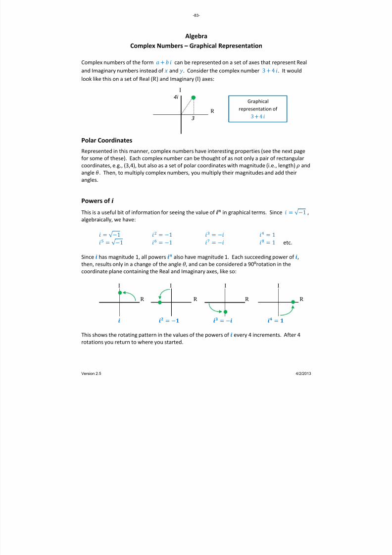
8/13/2019 AlgebraHandbook_very Helpful_ Print It
http://slidepdf.com/reader/full/algebrahandbookvery-helpful-print-it 83/178
Algebra Complex Numbers – Graphical Representation
Complex numbers of the form can be represented on a set of axes that represent Real
and Imaginary numbers instead of
and
. Consider the complex number
3 4 . It would
look like this on a set of Real (R ) and Imaginary (I) axes: I
4i R
3 Graphical
representation of
3 4
Polar Coordinates Represented in this manner, complex numbers have interesting properties (see the next page
for some of these). Each complex number can be thought of as not only a pair of rectangular
coordinates, e.g., (3,4), but also as a set of polar coordinates with magnitude (i.e., length) and
angle . Then, to multiply complex numbers, you multiply their magnitudes and add their
angles.
Powers of i This is a useful bit of information for seeing the value of in graphical terms. Since √ 1 , algebra have: ically, we
√ 1 1 1
√ 1
1 etc. 1Since has magnitude 1, all powers also have magnitude 1. Each succeeding power of ,
then, results only in a change of the angle θ, and can be considered a 90⁰rotation in the
coordinate plane containing the Real and Imaginary axes, like so:
I I I I
R R R R
This shows the rotating pattern in the values of the powers of every 4 increments. After 4
rotations you return to where you started.
-83-
Version 2.5 4/2/2013

8/13/2019 AlgebraHandbook_very Helpful_ Print It
http://slidepdf.com/reader/full/algebrahandbookvery-helpful-print-it 84/178
ADVANCED Algebra
Complex Number Operations in Polar Coordinates
Polar Coordinates
If a complex number is expressed in terms of its polar coordinates, many calculations are made
much easier. First, let’s investigate the relationship between a point’s rectangular coordinates
, and its pola coordinates , . r
The magnitude, ρ, is the distance of the point from the
origin: The angle, θ, is the angle the line from the point to the
origin makes with the positive portion of the x ‐axis.
Generally, this ot degrees. angle is expressed in radians, n
t a n or tan
Convers r coordin gular coordinates is straightforward: ion from pola ates to rectan
· c o s and · s i n
Example: In the illustration above, th shown has: e point
• Rectangular coordinates: 4,4
• Polar Coordinates:
4√ 2,
Complex Number Formulas: To see how useful this the r complex numbers: can be, consider following formulas fo
Multiplication: , · , · , So, to multiply r udes and add their angles.
Note on √ : Since i in polar coordinates is 1,
,
Using the root formula, √ 1 ,
In rectangular coordinates, then,
√ √ √
complex numbers, you multiply thei magnit
Division: , , , So, to divide complex n ide their magnitudes and subtract their angles. umbers, you div
Powers: , , · This results dire m ultiplication rule. ctly fro the m
Roots: , ,
ctly fro the poThis results dire m wer rule if the
exponent is a fraction.
-84-
Version 2.5 4/2/2013

8/13/2019 AlgebraHandbook_very Helpful_ Print It
http://slidepdf.com/reader/full/algebrahandbookvery-helpful-print-it 85/178
Algebra Complex Solutions to Quadratic Equations
Over the field of real numbers there are no roots to a quadratic function if the discriminant is
less than
zero.
Over
the
field
of
complex
numbers,
however,
such
a quadratic
function
has
two
roots.
Quadratic Refresher For a quadratic function of the form: The formula for the roots (i.e., where y = 0) is:
The discriminant is the part under the radical: How Many Roots? The following table tells us how many real or complex roots exist for a function, based on its
discriminant:
Note: because of the “” sign in the quadratic formula, when there are 2 complex roots they
are conjugates.
Valu o ant e f Discrimin Number of Roots
4 0 2 complex
4 0 1 real
4 0 2 real
Quadratic Formula
Example 1: 1 Solve 2 0 0 √ 42 2 2 411021 2 √ 362 2 6 2
Example : 2 Solve 2 4 7 0 √ 4
2 4 4 42722 4 √ 40
4 4 2√ 104 √
-85-
Version 2.5 4/2/2013

8/13/2019 AlgebraHandbook_very Helpful_ Print It
http://slidepdf.com/reader/full/algebrahandbookvery-helpful-print-it 86/178
Algebra Radical Rules
Simple Rules Involving Radicals G e eneral Radical Rul Ru u Roots le for Sq are Example
√ · √ √ · √ · √ · √ √ 12 √ 4 · √ 3 2√ 3
√ √ √ √ 54 √ 5√ 4 √ 52
Note also
that:
√ e.g., √ , so the rules for exponents also apply for roots.
Rationalizing the Denominator Mathematicians prefer to keep radicals out of the denominator. Here are two
methods to accomplish this, depending on what’s in the denominator.
Case 1: Simple radical in the denominator. Solution: multiply the beginning
expression by a frac h f radical ed by itself. tion w ich is the of ending divid
Example: √ √ √ √ · √ √ √ √
Case 2: Number and radical in the denominator. Solution: multiply by the
beginning expression by a fraction which is designed to eliminate the radical from
the denominator.
The
numerator
and
denominator
of
the
fraction
are
created
by
changing the sign between n be e othe um r and th radical in the den minator.
Example: √ √ √ √ · √ √ √ √ √ √
-86-
Version 2.5 4/2/2013

8/13/2019 AlgebraHandbook_very Helpful_ Print It
http://slidepdf.com/reader/full/algebrahandbookvery-helpful-print-it 87/178
Algebra Simplifying Square Roots – Two Methods
Method 1: Extracting Squares In this method, you pull squares out from under the radical. This is the quickest
method if you are comfortable with what the squares are and with dividing them
out of larger numbers. 11 121
12 144
13 169 14 196 15 225
16 256
17 289
18 324
19 36120 400
1 1
2 4
3 9
4 16
5 25
6 36
7 49
8 64
9
81
10 100
Examples: (1) √ 98 √ 49 · √ 2 7√ 2
(2) √ 9600 √ 100· √ 96· √ 16 · √ 6 100√ · √ 6 1 0 · 4
40√ 6
Method 2: Extracting Prime Numbers If
you
are
not
comfortable
with
Method
1,
you
can
pull
prime numbers out from under the radical and pair them
up to simplify t rhe square oot.
Example: √ 54 √ 2 · √ 27 √ 2 · √ 3 · √ 9 Method 2 may take a lot longer than
Method 1, but it works. A good use for
Method 2 is when you try using the
quicker Method 1 but get stuck – then
working with primes can get you back
on track
toward
solving
the
problem.
√ 2 · √ 3 · √ 3 · √ 3
√ 2 · √ 3 · √ 3 · √ 3
√ 2 · · √ 3 3 · √ 3 3 · √ 2 3 · √ 6 Note that the last step is to re‐combine roots
that do not come in pairs.
-87-
Version 2.5 4/2/2013
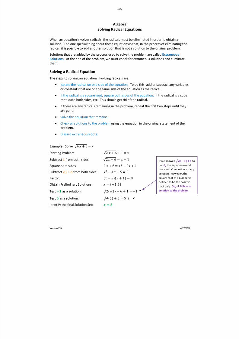
8/13/2019 AlgebraHandbook_very Helpful_ Print It
http://slidepdf.com/reader/full/algebrahandbookvery-helpful-print-it 88/178
Algebra Solving Radical Equations
When an equation involves radicals, the radicals must be eliminated in order to obtain a
solution. The one special thing about these equations is that, in the process of eliminating the
radical, it is possible to add another solution that is not a solution to the original problem.
Solutions that are added by the process used to solve the problem are called Extraneous Solutions. At the end of the problem, we must check for extraneous solutions and eliminate
them.
Solving a Radical Equation The steps to solving an equation involving radicals are:
• Isolate the radical on one side of the equation. To do this, add or subtract any variables
or constants that are on the same side of the equation as the radical.
• If the radical is a square root, square both sides of the equation. If the radical is a cube
root, cube both sides, etc. This should get rid of the radical.
• If there are any radicals remaining in the problem, repeat the first two steps until they
are gone.
• Solve the equation that remains.
• Check all solutions to the problem using the equation in the original statement of the
problem.
• Discard extraneous roots.
Example: Solve √ 4 5
Starting Problem: √ 2 6 1
Subtract 1 from both sides: 6√ 2 1
Square both i es: 1
If we allowed to
be -2, the equation would
work and -1 would work as a
solution. However, the
square root of a number is
defined
to
be
the
positive
root only. So, -1 fails as a solution to the problem.
s d 2 6 2Subtract from both sides: 0 4 5
Factor:
1 0
5 Obta reliminary Solutions:
in P 1,5
Test as a solution: 21 6 1Test as a solution: 5
1 ?
45 5 ?
Identify the final Solution Set:
-88-
Version 2.5 4/2/2013

8/13/2019 AlgebraHandbook_very Helpful_ Print It
http://slidepdf.com/reader/full/algebrahandbookvery-helpful-print-it 89/178
Algebra Algebra Solving Radical Equations (cont’d) Solving Radical Equations (cont’d)
Why Only Positive Square Roots? Why Only Positive Square Roots? It
is
generally
taught
in
high
school
algebra
that
square
roots
have
both
positive
and
negative
roots. So why are we now saying that the square root of a number is defined to be a positive
number only?
It is
generally
taught
in
high
school
algebra
that
square
roots
have
both
positive
and
negative
roots. So why are we now saying that the square root of a number is defined to be a positive
number only?
The answer lies in the missing step, which is often not taught to high school students. What
you learn is this:
The answer lies in the missing step, which is often not taught to high school students. What
you learn is this:
, . And, that is correct, but not because √ , . And, that is correct, but not because √ which it does not!
The Missing
Step
Starting Problem:
Take square roots: ||
Solve for x:
In the box to the right is the development with the
mis step cluded. Notice that: sing in
• √ || • When we take square roots, we have positive
numbers on each side of the resulting equation.
Both || and 2 are positive.
• The two possible values for x come from solving the middle equation || .
This solves
the
apparent
arbitrariness
of
when
a root
is
only
positive
and
when
it
is
both
positive and negative.
Inequalities
Starting Problem: 9
Take square roots:
|| 3
Case i Case ii and 3 3 3 3 and
Solution: | 3 3
The “missing step” also provides an explanation for the method used to solve inequalities.
Consider the inequality: 9. The process for solving this with the missing step included is:
Notice that || converts to in Case I and to
– in
Case
ii.
By
the
end
of
the
problem,
you
see that the sign in Case ii has been flipped
around from the original problem. This is not
magic; it is the result of “The Missing Step”
being applied in all its mathematical glory!
-89-
Version 2.5 4/2/2013

8/13/2019 AlgebraHandbook_very Helpful_ Print It
http://slidepdf.com/reader/full/algebrahandbookvery-helpful-print-it 90/178
Algebra
Matrix Addition and Scalar Multiplication
What is a Matrix?
A matrix is an ordered set of numbers set up in a 2‐dimensional array. Matrices are very useful
in algebra, statistics and other applications because they provide a concise way to carry out
more complex mathematical methods and processes.
Matrices have dimensions, expressed as the number of rows x the number of columns. For
example, a 2x3 matrix (read “2 by 3 matrix”) has 2 rows and 3 columns. Knowing the
dimensions of a matrix is important because many matrix operations can only occur on
matrices with certain dimensions.
Adding Matrices
Each number in a matrix is called an element. Matrices are added by adding the corresponding
elements in the matrices. Matrices must have the same dimensions to be added.
Example: 2 3 15 1 2 1 2 4 2 1 0 1 1 53 2 2 1st
row,
1st
column:
2 + (‐1) = 1
1st row, 2
nd column: (‐3) + 2 = ‐1
Scalar Multiplication
Multiplying a matrix by a scalar (i.e., a number) is accomplished by multiplying each element in
the matrix by the scalar. The term scalar simply refers to “scaling” the matrix by making its
values larger or smaller. Scalar multiplication can be performed on matrices of any dimensions.
Example:
3 ∙ 1 2 4 2 1 0 3 6 12 6 3 0 1st row, 1
st column: 3 ∙ (‐1) = ‐3
1st row, 2
nd column: 3 ∙ 2 = 6
-90-
Version 2.5 4/2/2013

8/13/2019 AlgebraHandbook_very Helpful_ Print It
http://slidepdf.com/reader/full/algebrahandbookvery-helpful-print-it 91/178
Algebra
Matrix Multiplication
Multiplying Matrices
Multiplication of matrices is a more complex process. Although the student may find it difficult
at first, it is a powerful tool that is useful in many fields of mathematics and science.
Matrix multiplication can be performed only on matrices that are conformable (i.e., compatible
in size). In order for two matrices to be multiplied together, the number of columns in the first
matrix must equal the number of rows in the second matrix. If an m x n matrix is multiplied by
an n x p matrix, the result is an m x p matrix. This is illustrated as follows:
∙ To multiply matrices, you multiply the elements in a row of one matrix by the corresponding
elements in a column of the other matrix and add the results. If row i in the first matrix is
multiplied by row j in the second matrix, the result is placed in row i , column j of the resulting
matrix. The element in position i, j of a matrix is often denoted ,. Example 1:
2 3 15 1 2 ∙ 1 2 2 1 3 1 1 01 1 3 1st row, 1
st column: [ 2 ∙ 1] + [ (‐3) ∙ 2] + [ 1 ∙ 3] = ‐1
1st row, 2
nd column: [ 2 ∙ (‐2) ] + [ (‐3) ∙ (‐1) ] + [ 1 ∙ 1] = 0
2nd
row, 1st column: [ 5 ∙ 1] + [ 1 ∙ 2] + [ (‐2) ∙ 3] = 1
2nd
row, 2nd
column: [ 5 ∙ (‐2) ] + [ 1 ∙ (‐1) ] + [ (‐2) ∙ 1] = ‐13Example 2:
1 22 13 1 ∙ 2 3 15 1 2 8 5 5 1 7 41 1 8 1
From the examples, it is clear that matrix multiplication is not commutative. That is, if we
name two matrices A and B, it is not necessarily true that A∙B = B∙ A. Further, if matrices are
not square (i.e., having the same number of rows and columns), matrix multiplication is never
commutative; that is A∙B ≠B∙ A.
size of resulting matrix
must match
Notice that multiplying a 2 x 3
matrix by
a 3 x 2
matrix
results
in a 2 x 2 matrix.
Notice that multiplying a 3 x 2
matrix by a 2 x 3 matrix results
in a 3 x 3 matrix.
-91-
Version 2.5 4/2/2013

8/13/2019 AlgebraHandbook_very Helpful_ Print It
http://slidepdf.com/reader/full/algebrahandbookvery-helpful-print-it 92/178
Algebra
Matrix Division and Identity Matrices
Multiplication and division are inverse processes with which the student is familiar when
working with
real
numbers.
Multiplication
of
matrices,
as
described
above
is
much
more
complex than multiplication of real numbers. So, how do you divide matrices?
Division of real numbers can be considered the process of multiplying a number by the inverse
of the number by which you want to divide. For example:
12 ∙ 4 (i.e., 12 divided by 3 is the same as 12 times ; the result is 4 either way)
dividing by 3 is the same a multiplying by the inverse of 3, which is
3
and
are
“multiplicative
inverses”
because
when
multiplied,
they
result
in
1,
which
is
called the “multiplicative identity”
Matrix division works in a similar fashion. First, we need to identify an identity matrix, then we
need to determine how to calculate an inverse matrix which, when multiplied by the original
matrix, results in the identity matrix. Only square matrices have inverses. Identity matrices
must also, by definition, be square.
Identity Matrices
Identity matrices exist for each square dimension. Identity matrices have 1’s down the diagonal
and 0’s in every other location. For example, the following are identity matrices, generally
denoted by the letter "": 1 00 1 1 0 00 1 00 0 1 1 00 1 0 00 00 00 0 1 00 1
When a matrix is multiplied by an identity matrix, the result is the original matrix.
Example: If we name a matrix , then ∙ ∙ as follows:
2 1 13 2 14 0 3 ∙ 1 0 00 1 00 0 1 1 0 00 1 00 0 1 ∙ 2 1 13 2 14 0 3 2 1 13 2 14 0 3
-92-
Version 2.5 4/2/2013
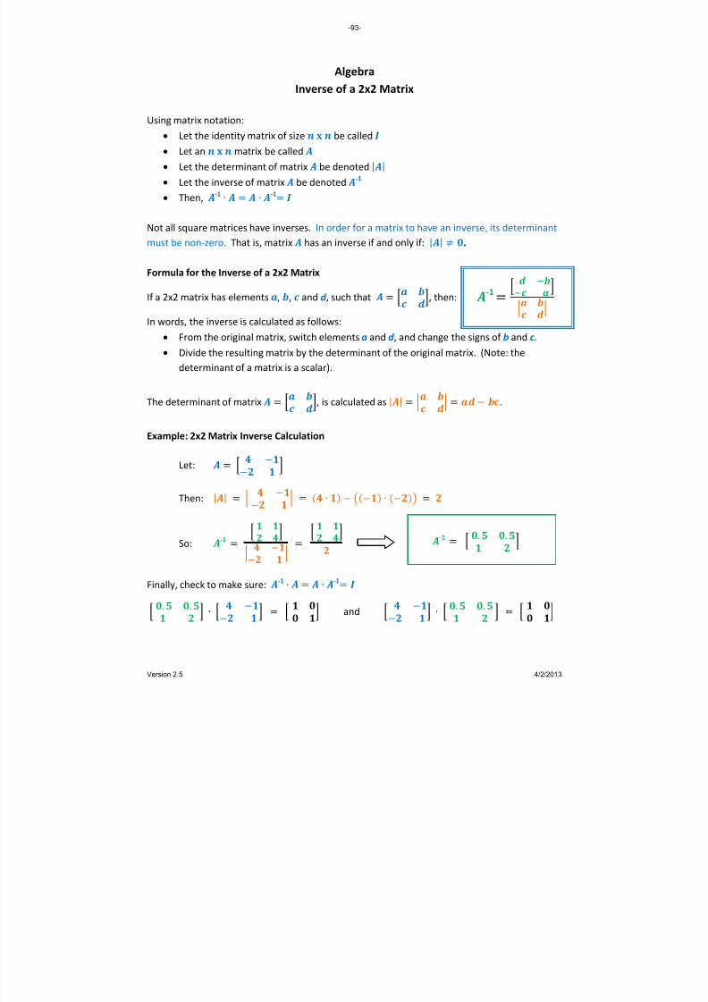
8/13/2019 AlgebraHandbook_very Helpful_ Print It
http://slidepdf.com/reader/full/algebrahandbookvery-helpful-print-it 93/178
Algebra
Inverse of a 2x2 Matrix
Using matrix notation:
Let the
identity
matrix
of
size
be
called
Let an matrix be called
Let the determinant of matrix be denoted | | Let the inverse of matrix be denoted ‐1
Then, ‐1 ∙ ∙ ‐1
Not all square matrices have inverses. In order for a matrix to have an inverse, its determinant
must be non‐zero. That is, matrix has an inverse if and only if: | | . Formula
for
the
Inverse
of
a 2x2
Matrix
If a 2x2 matrix has elements , , and d , such that , then: In words, the inverse is calculated as follows:
From the original matrix, switch elements a and d , and change the signs of b and c .
Divide the resulting matrix by the determinant of the original matrix. (Note: the
determinant of a matrix is a scalar).
The
determinant
of
matrix
,
is
calculated
as
| | .
Example: 2x2 Matrix Inverse Calculation
Let: Then: | | ∙ ∙
So:
‐
1
Finally, check to make sure: ‐1 ∙ ∙ ‐1
. . ∙ and ∙ . .
‐1
. .
‐1
-93-
Version 2.5 4/2/2013

8/13/2019 AlgebraHandbook_very Helpful_ Print It
http://slidepdf.com/reader/full/algebrahandbookvery-helpful-print-it 94/178
Algebra
Calculating Inverses – The General Case
The calculation of the inverse of a matrix of size greater than 2 x 2 can be performed by a
process called
Gauss
‐Jordan
Elimination.
The
process
is
also
called,
more
generically,
Row
Reduction. In this process, you begin with two side‐by‐side matrices, the one you want to
invert (the subject matrix) and the identity matrix of the same size. Operations are performed
on both matrices, gradually converting the original matrix to the identity Matrix.
Allowable operations are:
Multiplying or dividing a row by a scalar (i.e., a number).
Switching rows.
Adding or subtracting a multiple of one row to or from another.
When this process is complete, the original identity matrix has been converted to the inverse
matrix. Below is an example of the development of an inverse of a 3 x 3 matrix using this
process:
Start with the identity
matrix to the right of the
original subject matrix.
End with the inverse
matrix to the right of the
new identity matrix.
Each operation
performed on the original
subject matrix is also
performed on the original
identity matrix.
ADVANCED
-94-
Version 2.5 4/2/2013
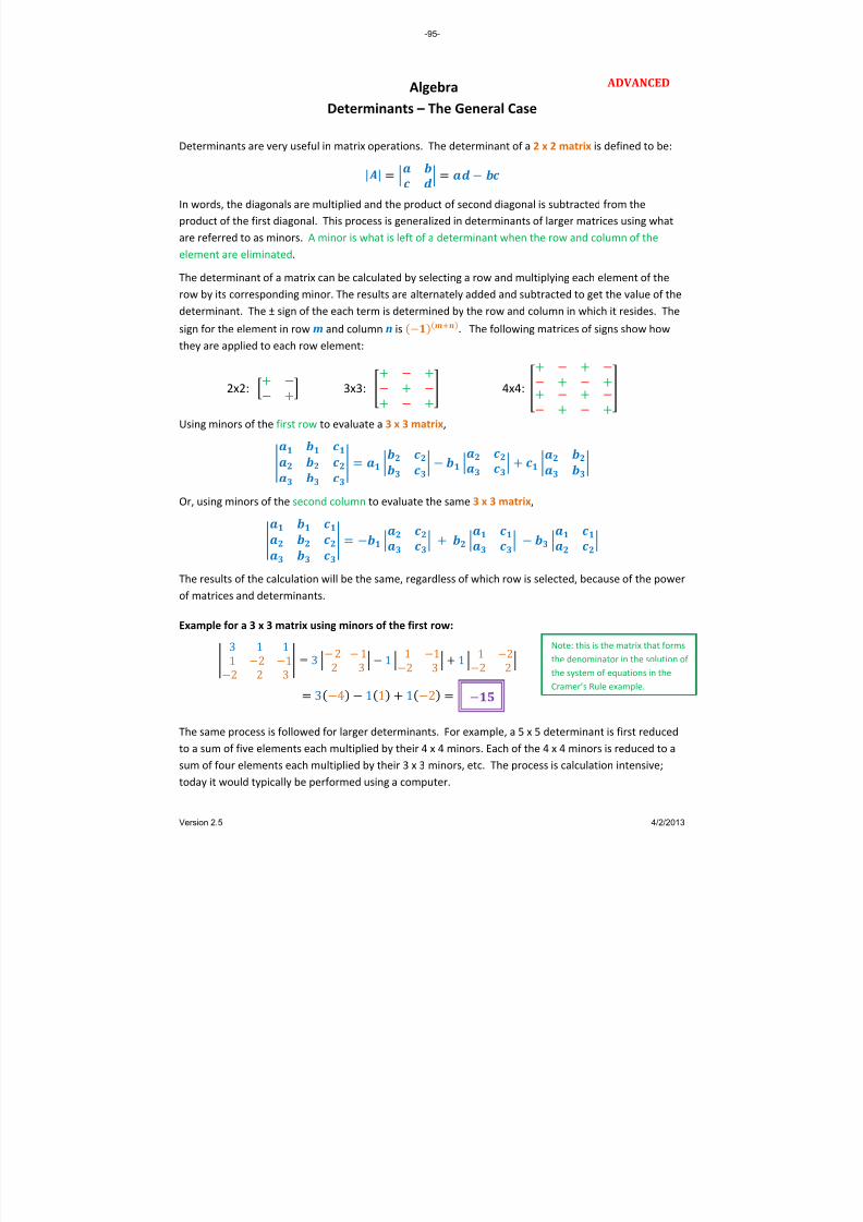
8/13/2019 AlgebraHandbook_very Helpful_ Print It
http://slidepdf.com/reader/full/algebrahandbookvery-helpful-print-it 95/178
Algebra
Determinants – The General Case
Determinants are very useful in matrix operations. The determinant of a 2 x 2 matrix is defined to be:
| |
In words, the diagonals are multiplied and the product of second diagonal is subtracted from the
product of the first diagonal. This process is generalized in determinants of larger matrices using what
are referred to as minors. A minor is what is left of a determinant when the row and column of the
element are eliminated.
The determinant of a matrix can be calculated by selecting a row and multiplying each element of the
row by its corresponding minor. The results are alternately added and subtracted to get the value of the
determinant. The ± sign of the each term is determined by the row and column in which it resides. The
sign for
the
element
in
row
m and
column
n is
. The following
matrices
of
signs
show
how
they are applied to each row element:
2x2: 3x3: 4x4:
Using minors of the first row to evaluate a 3 x 3 matrix,
Or,
using
minors
of
the
second
column
to
evaluate
the
same
3 x 3 matrix,
The results of the calculation will be the same, regardless of which row is selected, because of the power
of matrices and determinants.
Example for a 3 x 3 matrix using minors of the first row:
3 1 1 1 2 12 2 3 3 2 1 2 3 1 1 12 3 1 1 22 2 34 11 12
The same process is followed for larger determinants. For example, a 5 x 5 determinant is first reduced
to a sum of five elements each multiplied by their 4 x 4 minors. Each of the 4 x 4 minors is reduced to a
sum of four elements each multiplied by their 3 x 3 minors, etc. The process is calculation intensive;
today it would typically be performed using a computer.
Note: this is the matrix that forms
the denominator
in
the
solution
of
the system of equations in the
Cramer’s Rule example.
ADVANCED
-95-
Version 2.5 4/2/2013

8/13/2019 AlgebraHandbook_very Helpful_ Print It
http://slidepdf.com/reader/full/algebrahandbookvery-helpful-print-it 96/178
Algebra
Cramer’s Rule – 2 Equations
Cramer’s Rule provides a powerful and simple way to solve systems of two or three linear
equations. In
larger
systems
of
equations,
it
is
a useful
way
to
solve
for
just
one
of
the
variables, without having to solve the entire system of equations. To solve an entire system of
four or more equations, a better technique would be Gauss‐Jordan Elimination, especially if the
student is aided by a computer and spreadsheet software such as Microsoft Excel.
Cramer’s Rule works as long as the determinant of variable coefficients (i.e., the determinant in
the denominator) is non‐zero. If this determinant is zero, then there is no unique solution to
the system of equations.
General Case for 2 Equations in 2 Unknowns
The standard form of the equations is:
Using determinant notation, Cramer’s Rule states that the solutions for x and y are:
Notice that the determinants in the denominators are the same; the columns in these
determinants are the coefficients of the variables in the equations. The determinants in the
numerators are almost the same as the ones in the denominators; the only difference is that
the column of coefficients associated with the variable being evaluated is replaced by the
equations’ constant terms.
Example: Consider these equations:
3 6 18
3 7
Then,
123
-96-
Version 2.5 4/2/2013

8/13/2019 AlgebraHandbook_very Helpful_ Print It
http://slidepdf.com/reader/full/algebrahandbookvery-helpful-print-it 97/178
Algebra
Cramer’s Rule – 3 Equations
General Case for 3 Equations in 3 Unknowns
The standard form of the equations is:
Using determinant notation, Cramer’s Rule states that the solutions for x, y and z are:
As in the case with two equations, the determinants in the denominators are all the same; the
columns in these determinants are the coefficients of the variables in the equations. The
determinants in the numerators are almost the same as the ones in the denominators; the only
difference is that the column of coefficients associated with the variable being evaluated is
replaced by the equations’ constant terms.
Example: Consider these equations:
3 7
2 2 2 2 3 4
Using determinant notation:
Performing the required calculations, we obtain the unique solution:
Note that the determinant of
variable coefficients must be non‐
zero in order to use Cramer’s
Rule. If this determinant is zero,
there is no unique solution to the
system of equations.
2 3 2
ADVANCED
-97-
Version 2.5 4/2/2013

8/13/2019 AlgebraHandbook_very Helpful_ Print It
http://slidepdf.com/reader/full/algebrahandbookvery-helpful-print-it 98/178
Algebra
Augmented Matrices
Solving Simultaneous Equations
One relatively
advanced
method
of
solving
simultaneous
equations
is
through
the
use
of
an
Augmented Matrix. A matrix is considered augmented if it consists of the matrix of the
coefficients of the variables, augmented by the constant terms. In order for a system of
equations to be solved in this form, they must be written in standard form.
Example:
Gauss‐Jordan Elimination
A process called Gauss‐Jordan Elimination (GJE) is used to manipulate the augmented matrix to
obtain a solution to the equations. GJE is also called Row Reduction because each step adjusts
the values in one row of the augmented matrix. At the end of the process, the rows of the
coefficient matrix are “reduced” to the Identity Matrix.
The following manipulations of the rows are allowed:
Multiplying or dividing a row by a scalar (i.e., a number).
Switching rows.
Adding or subtracting a multiple of one row to or from another.
When this process is complete, the constant column of the augmented matrix has been
converted to the solution of the system of equations. Why does this work? The process used is
essentially the same as solving a system of equations by the elimination method. In GJE, you
ignore the variable names by using matrices, but the manipulations are the same.
Inverse Matrix
This process
can
also
be
used
to
develop
an
Inverse
Matrix.
To
do
this,
Place an identity matrix to the right of the augmented matrix at the start.
Perform all row operations on this matrix as you progress.
At the end, the original identity matrix will have been converted to the inverse matrix.
In the following examples, augmented matrices are manipulated to develop solutions to
systems of equations and identity matrices are converted to inverse matrices.
ADVANCED
1 3 132 1 4 The augmented
matrix would be:
To solve the
system:
3 13 2 4
-98-
Version 2.5 4/2/2013

8/13/2019 AlgebraHandbook_very Helpful_ Print It
http://slidepdf.com/reader/full/algebrahandbookvery-helpful-print-it 99/178
Action Taken Why?
Start x y =Starting Augmented Matrix 2 8 36 1 0
1 5 10 0 1
Adjust Top Row
(Row 1) ÷ (a11) ‐‐> Row 1 To get a "1" in column 1 1 4 18 0.5 0
Row2 (no change) 1 5 10 0 1
Adjust 2nd Row
Row1 (no change) 1 4 18 0.5 0
(Row 2) ‐ (a21 * Row 1) ‐‐> Row 2 To get a "0" in column 1 0 1 ‐8 ‐0.5 1
Adjust 2nd Row
Row1 (no change) 1 4 18 0.5 0
(Row 2) ÷ (a22) ‐‐> Row 2 To get a "1" in column 2 0 1 ‐8 ‐0.5 1
Adjust Top Row
(Row 1)
‐(a12
* Row
2)
‐‐> Row
1 To
get
a "0"
in
column
2 1 0 50
= x 2.5
‐4
Row2 (no change) 0 1 ‐8 = y ‐0.5 1
Matrix Inverse Test
2 8 2.5 ‐4 1 0
1 5 ‐0.5 1 0 1
Action Taken Why?
Start x y =
Starting Augmented Matrix ‐1 3 13 1 0
2 ‐1 4 0 1
Adjust Top Row
(Row 1) ÷ (a11) ‐‐> Row 1 To get a "1" in column 1 1 ‐3 ‐13 ‐1 0
Row2 (no change) 2 ‐1 4 0 1
Adjust 2nd Row
Row1 (no change) 1 ‐3 ‐13 ‐1 0
(Row 2) ‐ (a21 * Row 1) ‐‐> Row 2 To get a "0" in column 1 0 5 30 2 1
Adjust 2nd Row
Row1 (no
change) 1
‐3
‐13
‐1 0
(Row 2) ÷ (a22) ‐‐> Row 2 To get a "1" in column 2 0 1 6 0.4 0.2
Adjust Top Row
(Row 1) ‐ (a12 * Row 2) ‐‐> Row 1 To get a "0" in column 2 1 0 5 = x 0.2 0.6
Row2 (no change) 0 1 6 = y 0.4 0.2
Matrix Inverse Test
‐1 3 0.2 0.6 1 0
2 ‐1 0.4 0.2 0 1
Original Matrix Inverse Matrix Product Matrix
Inverse MatrixOriginal Matrix Product Matrix
Problem: solve the following set of simultaneous equations using row reduction
(formally called Gauss‐Jordan Elimination)
‐x + 3y = 13
2x ‐ y = 4
Algebra
2x2 Augmented Matrix Examples
Augmented Matrix Inverse
Matrix
Inverse Matrix
Inverse Matrix
Inverse Matrix
Augmented Matrix
Problem: solve the following set of simultaneous equations using row reduction
(formally called Gauss‐Jordan Elimination)
2x + 8y = 36
x + 5y = 10
-99-
Version 2.5 4/2/2013

8/13/2019 AlgebraHandbook_very Helpful_ Print It
http://slidepdf.com/reader/full/algebrahandbookvery-helpful-print-it 100/178
Action Taken Why?
Starting Augmented
Matrix x y z =
Starting Augmented Matrix 2 ‐1 3 ‐7
1 4 ‐2 17
3 1 2 2
Work Down
Row1 * 1/2 ‐‐> Row1 To get a "1" in column 1 1 ‐0.5 1.5 ‐3.5
Row2 ‐ (new Row1) ‐‐> Row2 To get a "0" in column 1 0 4.5 ‐3.5 20.5
Row3 ‐ (3 * new Row1) ‐‐> Row 3 To get a "0" in column 1 0 2.5 ‐2.5 12.5
Work Down
Row1 (no change) 1 ‐0.5 1.5 ‐3.5
Switch Rows 2 and 3 New Row2 looks easier to work with 0 2.5 ‐2.5 12.5
Switch Rows 2 and 3 New Row2 looks easier to work with 0 4.5 ‐3.5 20.5
Work Down
Row1 (no change) 1 ‐0.5 1.5 ‐3.5
Row2 / 2.5 ‐‐> Row2 To get a "1" in column 2 0 1 ‐1 5
Row3 * 2 ‐‐> Row3 To get rid of the fractions 0 9 ‐7 41
Work Down
Row1 (no change) 1 ‐0.5 1.5 ‐3.5
Row2 (no change) 0 1 ‐1 5
Row3 ‐ (9 * Row2) ‐‐> Row 3 To get a "0" in column 2 0 0 2 ‐4
Work Down
Row1 (no change) 1 ‐0.5 1.5 ‐3.5
Row2 (no change) 0 1 ‐1 5
Row3 * .5 ‐‐> Row3 To get a "1" in column 3 0 0 1 ‐2
Work Up
Row1 ‐ (Row3 * 1.5) ‐‐> Row1 To get a "0" in column 3 1 ‐0.5 0 ‐0.5
Row2 + Row3 ‐‐> Row2 To get a "0" in column 3 0 1 0 3
Row3 (no
change) 0 0 1
‐2
Work Up
Row1 + (Row2 * .5) ‐‐> Row1 To get a "0" in column 2 1 0 0 1 = x
Row2 (no change) 0 1 0 3 = y
Row3 (no change) 0 0 1 ‐2 = z
Matrix Inverse Test
2 ‐1 3 ‐2 ‐1 2 1 0
1 4 ‐2 1.6 1 ‐1.4 0 1
3 1 2 2.2 1 ‐1.8 0 0
Inverse Matrix Product MaOriginal Matrix
2x ‐ y + 3z = ‐7
x + 4y ‐2z = 17
3x +y +2z = 2
Problem: solve the following set of simultaneous
equations using row reduction (formally called
Gauss‐Jordan Elimination)
Algebra
3x3 Augmented Matrix Example
Augmented Matrix
-100-
Version 2.5
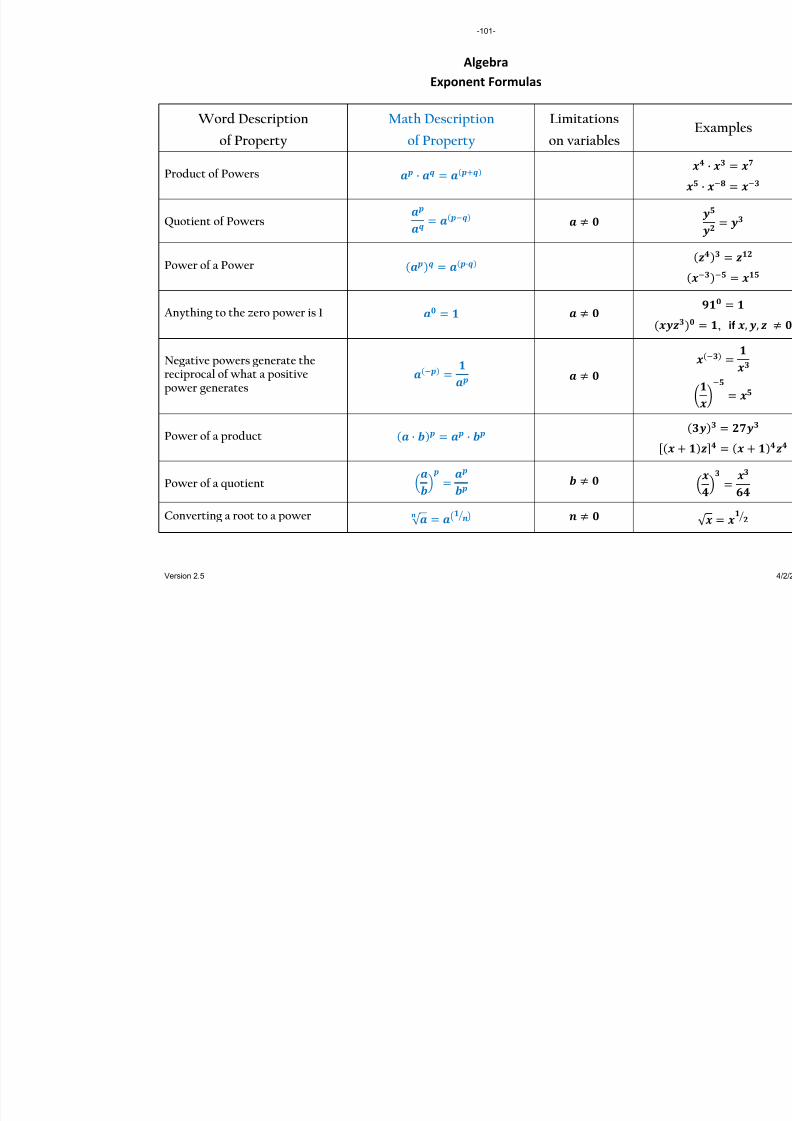
8/13/2019 AlgebraHandbook_very Helpful_ Print It
http://slidepdf.com/reader/full/algebrahandbookvery-helpful-print-it 101/178
Algebra Exponent Formulas
Word Description
of Property
Math Description
of Property
Limitations
on variables
Product of Powers ·
Quotient of Powers
Power of a Power ·
Anything to the zero power is 1
Negative powers generate thereciprocal of what a positivepower generates
Power of a product · ·
Power of a quotient
Converting a root to a power √
-101-
Version 2.5
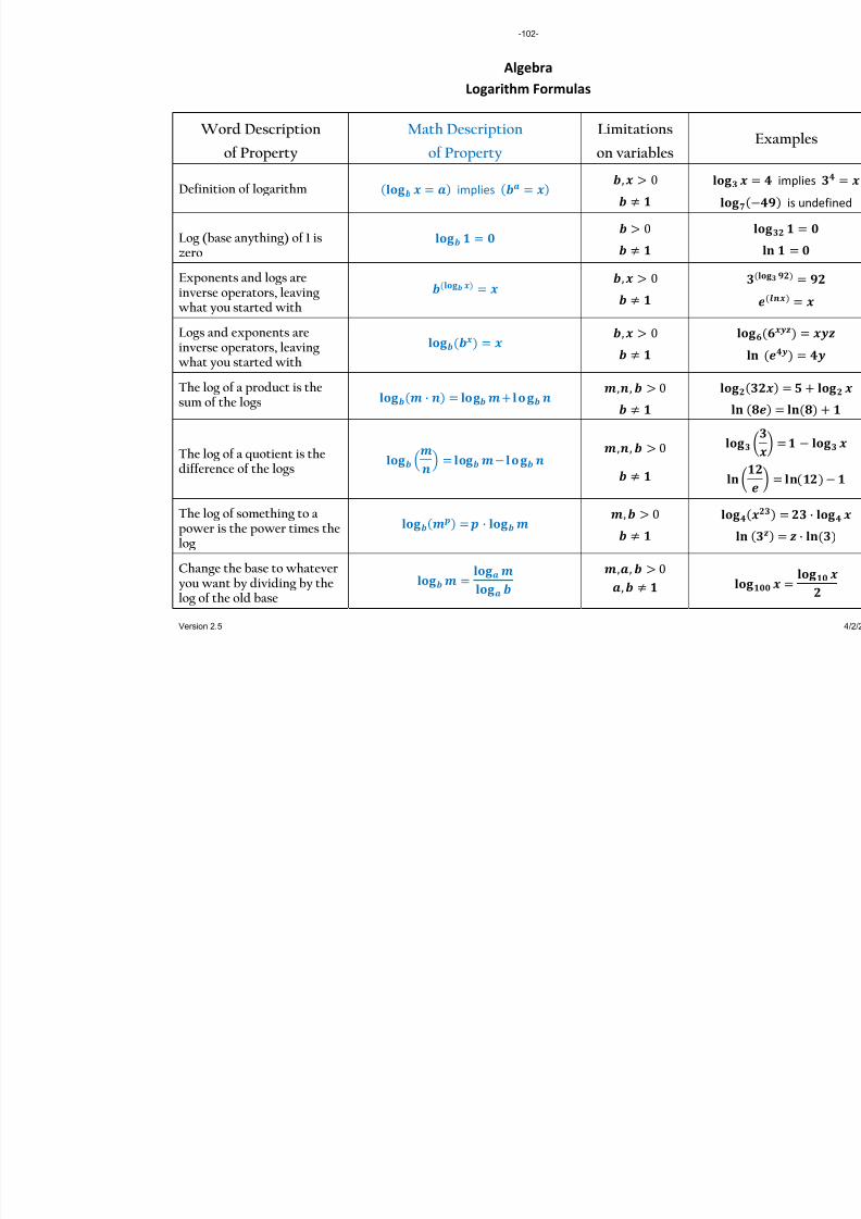
8/13/2019 AlgebraHandbook_very Helpful_ Print It
http://slidepdf.com/reader/full/algebrahandbookvery-helpful-print-it 102/178
Algebra Logarithm Formulas
Word Description
of Property
Math Description
of Property
Limitations
on variables
Definition of logarithm implies , 0
Log (base anything) of 1 iszero
0
Exponents and logs areinverse operators, leavingwhat you started with
, 0
Logs and exponents areinverse operators, leavingwhat you started with
, 0
The log of a product is thesum of the logs ·
,, 0
The log of a quotient is thedifference of the logs
,, 0
The log of something to apower is the power times thelog
· , 0
Change the base to whateveryou want by dividing by thelog of the old base
,, 0
,
-102-
Version 2.5

8/13/2019 AlgebraHandbook_very Helpful_ Print It
http://slidepdf.com/reader/full/algebrahandbookvery-helpful-print-it 103/178
ADVANCED Algebra
e What is “e”?
e is a transcendental number, meaning that it is not the root of any polynomial with
integer coefficients.
e is the base of the natural logarithms.
What Makes “e” so Special? e shows up over and over in mathematics, especially in regard to limits, derivatives, and
integrals.
In
particular,
it
is
noteworthy
that:
lim→ 1 1 lim→ √ !
1
Perhaps, most interestingly, the following equation, called Euler’s Equation, relates five
seemingly unrelated mathematical constants to each other.
Some Series Representations of e
1!
1 1 12 16 124 1120 ⋯
1!
1
1 1 1
2 1
6 1
24 1
120 ⋯
Decimal Expansion 2.7 1828 1828 4590 4523 5360 2874 7135 2662 4977 5724 7093 6999 5957 4966 …The web site http://antwrp.gsfc.nasa.gov/htmltest/gifcity/e.2mil shows the decimalexpansion of e to over 2 million digits.
There are many more series involving e.
A sampling of these is provided at:
http://mathworld.wolfram.com/e.html.
-103-
Version 2.5 4/2/2013

8/13/2019 AlgebraHandbook_very Helpful_ Print It
http://slidepdf.com/reader/full/algebrahandbookvery-helpful-print-it 104/178
Algebra Table of Exponents and Logarithms
024
Definition:
if and only if
-104-
Version 2.5 4/2/2013
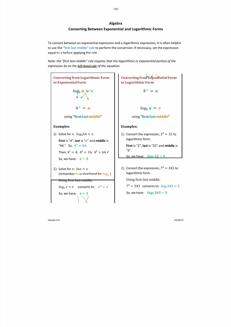
8/13/2019 AlgebraHandbook_very Helpful_ Print It
http://slidepdf.com/reader/full/algebrahandbookvery-helpful-print-it 105/178
Algebra Converting Between Exponential and Logarithmic Forms
To
convert
between
an
exponential
expression
and
a
logarithmic
expression,
it
is
often
helpful
to use the “first‐last‐middle” rule to perform the conversion. If necessasy, set the expression
equal to before applying the rule.
Note: the “first ‐last ‐middle” rule requires that the logarithmic or exponential portion of the
expression be on the left ‐hand side of the equation.
Converting from Exponential Form
to Logarithmic Form
using “first ‐last ‐middle”
Examples:
1 Convert the expression,
2 32 to
logarithmic form.
First is “2”, last is “32” and middle is
“5”.
So, we have:
2 Convert the expression, 7 343 to
logarithmic form.
Using first‐last‐middle,7 343 converts to: 343 3
So, we have:
Converting from Logarithmic Form
to Exponential Form
using “first ‐last ‐middle”
Examples:
1) Solve for
: 64 . First is “4”, last is “” and middle is
“64.” So, 4 64. Then, 4 4; 4 16; 4 64
So, we have: 2 Solve for : ln
(remember
is shorthand for
)
Using first‐last‐middle, converts to:
So, we have:
-105-
Version 2.5 4/2/2013

8/13/2019 AlgebraHandbook_very Helpful_ Print It
http://slidepdf.com/reader/full/algebrahandbookvery-helpful-print-it 106/178
Algebra Expanding Logarithmic Expressions
Expanding a logarithmic expression is a process best described by example. Each step of the
process is described and illustrated in the example below.
Expand:
Step 1: Simplify terms in the original expression, if possible:
Step 2: Write the log of all of the items in parentheses in the simplified expression:
2 3
Step 3: Write the exponents from the simplified expression as coefficients of each log:
2 3
Step 4: Write the signs (“” for items in the numerator; ““ for items in the denominator):
2 3 2 3 4
Step 5: Simplify terms
in
the
solution,
if possible:
1 3 2 3 4
Result: 1 3 2 3 4
When expanded:
Each item in the numerator will become a term preceded by a “+” sign
Each item in the denominator will become a term preceded by a “‐” sign.
All exponents become term coefficients in expanded form.
-106-
Version 2.5 4/2/2013

8/13/2019 AlgebraHandbook_very Helpful_ Print It
http://slidepdf.com/reader/full/algebrahandbookvery-helpful-print-it 107/178
Algebra Condensing Logarithmic Expressions
Condensing a logarithmic expression is a process best described by example. Each step of the
process is described and illustrated in the example below.
Condense: 1 2 2 3 4
Step 1: Review the expression and identify each element.
The argument of each log will become the base of an exponential term.
The coefficient of each log will become an exponent on that term
The sign of each term determines whether the exponential term goes in the
numerator (+) or denominator of the condensed expression.
1 2 2 3 4
Step 2: Set up the log expression with the proper base and parentheses to contain the various
terms. If
there
is
at
least
one
negative
sign,
set
up
a fraction
inside
the
parentheses:
Step 3: Convert any constants to powers of the base of the log:
… Step 4: Bring in each term containing a variable as an exponential expression with the proper
exponent and
base:
Step 5: Simplify to the extent possible:
∙
“‐“ indicates that a term
goes in the denominator
“+” indicates that a term
goes in the numerator
exponents When condensed, each term will
become exponential in form. All
terms in the numerator will be
multiplied together. All terms in
the denominator will be multiplied
together.
-107-
Version 2.5 4/2/2013

8/13/2019 AlgebraHandbook_very Helpful_ Print It
http://slidepdf.com/reader/full/algebrahandbookvery-helpful-print-it 108/178
Algebra Condensing Logarithmic Expressions – More Examples
Suggestions for doing problems: Use parentheses liberally to help yourself see what is going on in the problem. Do the problems one step at a time, working carefully down the page. Leave yourself a lot of room to do the work; there may be a lot of steps.
Some additional examples to help see how the various rules fit together:
8log 14 log 2 log log ∙ 6 ln3 6 ln 3 ln 11 ln 3
2 3 ∙ log log 1 log16 log 0 log16
log log loglog100 log
32 log
log 116 6 2 4 6
-108-
Version 2.5

8/13/2019 AlgebraHandbook_very Helpful_ Print It
http://slidepdf.com/reader/full/algebrahandbookvery-helpful-print-it 109/178
Algebra Graphing an Exponential Function
Graphing an exponential or logarithmic function is a process best described by example. Each
step of
the
process
is
described
and
illustrated
in
the
examples
over
the
next
few
pages.
Graph the function:
Step 2: Select points for the graph:
0 3 2 1.67
1 3 2 1
2 3 2 1
Step 3: Graph the exponential function:
In selecting points for an
exponential curve, good
choices often relate to the
value of the exponent.
Choose values that make
the exponent ‐1, 0 and 1; or
‐1, 0 and 2.
In this example, select so that:
1 1 so, 0
1 0 so, 1
1 1 so, 2
3C: Sketch in the curve 3A: Graph the asymptote 2 3B: Graph the points
Step 1: The horizontal asymptote occurs at the
value of the constant term. This is because the
exponential term approaches zero as the
exponent becomes more and more negative.
is the asymptote.
-109-
Version 2.5 4/2/2013

8/13/2019 AlgebraHandbook_very Helpful_ Print It
http://slidepdf.com/reader/full/algebrahandbookvery-helpful-print-it 110/178
Four Exponential Function Graphs Impact of varying base (above 1 and below 1)
Note: exponential and logarithmicfunctions that are inverses ofeach other (on this page and theone following) are the same color.
-110-
Version 2.5 4/2/2013

8/13/2019 AlgebraHandbook_very Helpful_ Print It
http://slidepdf.com/reader/full/algebrahandbookvery-helpful-print-it 111/178
Algebra Graphing a Logarithmic Function
Method 1:
Direct
Method
Graph the sample Function: 1 3
Step 2: Select points for the graph: In selecting points for a logarithmic curve, good choices often relate to the value of the argument.
Choose values that make the argument 1 and the base of the logarithm (1 and 4 in this example).
2 2 1 3 1 3
5 5 1 3 4 3
Step 3: Graph the logarithmic function:
3C: Sketch in the curve
In this example, select so that:
1 1 so, 2
1 4 so, 5
See what happens when we do this
in the table to the right:
3A: Graph the asymptote 1 3B: Graph the points
Step 1: Find the vertical asymptote at the value of
x that makes the argument of the log zero.
1 0 so, is the asymptote.
Note that two points may be sufficient to graph the curve if we have also drawn the asymptote.
By selecting x’s so that the values in parentheses are 1 and
the base of the log, the calculation of y’s becomes easy.
-111-
Version 2.5 4/2/2013

8/13/2019 AlgebraHandbook_very Helpful_ Print It
http://slidepdf.com/reader/full/algebrahandbookvery-helpful-print-it 112/178
Algebra Graphing a Logarithmic Function (cont’d)
Natural Logarithm Notation:
…
"ln" stands for “logarithmus naturalis” (Latin for “natural logarithm”) and is the logarithm with base "". The “ln” notation was invented in the late 1800’s, when a lot of work was done by hand (there were no
electronic calculators or computers). Those who worked with logarithms often used natural logarithms
extensively, so this shorthand notation became quite popular, and has survived to this day. So, when you see: ln … think log … .
Method 1: Direct Method when the base of the logarithm is “”
Step 2: Select points for the graph: In selecting points for a logarithmic curve, good choices often relate to the value of the argument.
Choose values that make the argument 1 and the base of the logarithm (1 and e in this example).
2
ln 2 1 3 ln 1 3
3.7 ln 1 1 3 ln 3
Step 3: Graph the logarithmic function:
3C: Sketch in the curve
In this example, select so that:
1 1 so,
2
1 e so, 1
You need to know that ~ 2.7. So, 1 ~ 3.7.
3A: Graph the asymptote
1 3B: Graph the points
Step 1: Find the vertical asymptote at the value of
x that
makes
the
argument
of
the
log
zero.
1 0 so, is the asymptote.
Note that two points may be sufficient to graph the curve if we have also drawn the asymptote.
By selecting x’s so that the values in parentheses are 1 and
the base of the log, the calculation of y’s becomes easy.
-112-
Version 2.5 4/2/2013

8/13/2019 AlgebraHandbook_very Helpful_ Print It
http://slidepdf.com/reader/full/algebrahandbookvery-helpful-print-it 113/178
Algebra Graphing a Logarithmic Function (cont’d)
Method 2:
Double
‐Inverse
Method
Step 1: Find the inverse function:
Switch variables: 1 3
Subtract the constant: 3 3
Result: 3 1
Take powers of the log base: 4 4
Simplify: 4 1
Subtract the
constant:
1 1
Resulting INVERSE Function: 4 1 or
Step 3: Select points for the graph:
2 4 1 1.25
3 4 1 2
4
4 1 5
Step 4: Switch the x and y values to get points for the logarithmic function:
.
Step 5: Graph the logarithmic function:
5C: Sketch in the curve
In selecting points for an
exponential curve, good
choices often relate to the
value of the exponent.
Choose values that make
the exponent
‐1,
0 and
1;
or
‐1, 0 and 2.
In this example, select so that:
3 1 so, 2
3 0 so, 3
3 1 so,
4
5A: Graph the asymptote 1 5B: Graph the points
Step 2: Find the vertical asymptote at the value of x
that makes the argument of
the log zero.
1 0so, is the asymptote.
-113-
Version 2.5 4/2/2013

8/13/2019 AlgebraHandbook_very Helpful_ Print It
http://slidepdf.com/reader/full/algebrahandbookvery-helpful-print-it 114/178
Four Logarithmic Graphs Impact of varying base (above 1 and below 1)
⁄
Note: exponential and
are inverses of each o
on this one) are the sa
-114-
Version 2.5

8/13/2019 AlgebraHandbook_very Helpful_ Print It
http://slidepdf.com/reader/full/algebrahandbookvery-helpful-print-it 115/178
Algebra
Gra hs of Various Functions
10.0
y = 2x
10.0
y = (½)x
‐5.0
0.0
5.0
‐10.0 ‐5.0 0.0 5.0 10.0
‐5.0
0.0
5.0
‐10.0 ‐5.0 0.0 5.0 10.0
‐10.0 ‐10.0
y = log2 x y = log½ x
0 0
5.0
10.0
0.0
5.0
10.0
‐10.0
‐5.0
.
‐10.0 ‐5.0 0.0 5.0 10.0
‐10.0
‐5.0
.
‐10.0 ‐5.0 0.0 5.0 10.0
5.0
10.0
y = x½
5.0
10.0
y = x2
5.0
10.0
y = x3
‐10.0
‐5.0
0.0
‐10.0 ‐5.0 0.0 5.0 10.0
‐10.0
‐5.0
0.0
‐10.0 ‐5.0 0.0 5.0 10.0
‐10.0
‐5.0
0.0
‐10.0 ‐5.0 0.0 5.0 10.0
-115-
Version 2.5 4/2/2013

8/13/2019 AlgebraHandbook_very Helpful_ Print It
http://slidepdf.com/reader/full/algebrahandbookvery-helpful-print-it 116/178
Algebra Applications of Exponential Functions
Exponential Growth and Decay
∙ 1
∙ 1
Interest Formulas
Let:
= Amount of money at time
= Principal (starting amount of money); note that 0 = the annual rate of interest (e.g., 4% or .04) = the number of times per year that interest is credited
Compound interest pays interest a number of times during the year; that is, in
periods after the first, interest is paid on the original amount invested plus
interest earned in prior periods.
Compound interest
paid
n times
a year:
∙
Simple case. If interest is compounded on an annual basis, we get the simplest
formula:
Annual interest paid once a year: ∙
Continuous compounding. The
more
frequent
the
compounding
of
interest,
the
more money you get. The best return on your money occurs if interest is
compounded continuously. Because of the definition of the mathematical
constant "", we get the following formula (known as the “Pert” formula).
Interest compounded continuously: ∙
Note: if you let the end value be
represented by and the
start value by , you get similar
formulas to the interest
formulas below.
-116-
Version 2.5 4/2/2013

8/13/2019 AlgebraHandbook_very Helpful_ Print It
http://slidepdf.com/reader/full/algebrahandbookvery-helpful-print-it 117/178
Example: Start: 1
log 1 1
Add 1: log 1 2
Multiply by
: log 1 3
Exponentiate: 2 2
Simplify: 1 8
Subtract 1:
Example: Start:
2 4 ∙ 3
110
Subtract 2: 4 ∙ 3 108
Divide by 4: 3 27
Take logs: log3 log27
Simplify: 2 3
Add 2:
Algebra Solving Exponential and Logarithmic Equations
Logarithms and exponents are inverse operations in the same way addition and subtraction are,
and in
the
same
way
multiplication
and
division
are.
So,
to
undo
an
exponent,
you
take
a
logarithm, and to undo a logarithm, you take an exponent.
Solving an Exponential Equation Sometimes an equation has a variable in an exponent. To solve this kind of equation, follow
these steps:
Isolate the term with the exponent on one side
of the equation. That is, undo any additions,
subtractions, multiplications,
and
divisions
in
the equation.
Take a logarithm of both sides of the equation.
Use the base that exists in the exponential
term.
Solve the equation that remains.
Note: in the example at right, the base of 3 is selected
for the logarithms because it is the base of the exponent in the problem.
Solving a Logarithmic Equation To solve an equation with a logarithm in it, follow these steps:
Isolate the logarithm on one side of the
equation. That is, undo any additions,
subtractions, multiplications, and divisions in
the equation.
Take the base of the logarithm to the power of
both sides
of
the
equation.
Use
the
same
base
that exists in the logarithmic term.
Solve the equation that remains.
Note: in the example at right, the base of 2 is selected
for use in exponentiation because it is the base of the
logarithm in the problem.
-117-
Version 2.5 4/2/2013

8/13/2019 AlgebraHandbook_very Helpful_ Print It
http://slidepdf.com/reader/full/algebrahandbookvery-helpful-print-it 118/178
Algebra Polynomial Function Graphs
Definitions • Local Maximum
–
The
largest
value
that
a function
takes
in
a neighborhood
around
the
point. There must be smaller values on both sides of the local maximum.
• Local Minimum – The smallest value that a function takes in a neighborhood around the
point. There must be larger values on both sides of the local minimum.
• A function is Increasing over an interval if it
generates larger values as x increases over the
same interval.
• A function is Decreasing over an interval if it
generates smaller
values
as
x
increases
over
the
same interval.
The graph at the right has two local maxima and two local
minima. It also has three intervals where it is increasing
and two intervals where it is decreasing.
Characteristics of the Graph f a Polynomial o
If
olynomial of degree
, then … is a p
• is continuous ov values of x . er all
• Roots (i.e., zeroes) of exist wherever the graph intersects the x ‐axis. There are at
most of them.
• The y ‐intercept of the graph occurs at 0, which is the constant term of the
omial. polyn
• will have at most 1 local extrema (either maxima or minima). For example, a
5th
degree polynomial will have at most 4 extrema; the example above has 4 extrema.
• At each extreme, the slope of a line tangent to the curve will be zero. However, if the
slope of the tangent line to the curve at a point is zero, the point is not necessarily an
extreme.
• At a local maximum, the polynomial must be increasing on the left and decreasing on
the right.
• At a local minimum, the polynomial must be decreasing on the left and increasing on
the right.
-118-
Version 2.5 4/2/2013

8/13/2019 AlgebraHandbook_very Helpful_ Print It
http://slidepdf.com/reader/full/algebrahandbookvery-helpful-print-it 119/178
ADVANCED Algebra
Finding Extrema with Derivatives Derivatives The derivative of a monomial is:
The notation
means “take a derivative with respect to the variable x .” We need to know two
other things about derivatives in order to find extrema with them.
• The derivative of a sum t is he sum of the derivatives. That is:
• Derivatives provide
information
about
the
slopes
of
lines
tangent
to
the
curve
at
each
point. Since the slope of a tangent line at a minimum or maximum is zero, we can
calculate the derivative of a polynomial and set it equal to zero to find the x ‐values of its
extrema.
Finding Extrema with Derivatives If is a polynomial, any extrema lie at points where
Example 1: Take the general quadratic equation:
.
We know that the graph of this equation has a single maximum or minimum which is the vertex
of the parabola. Taking a deriv ti f l ual to zero, we get: a ve o this formu a and setting it eq
Solving for x , we get : , which we already know is the x‐value of the vertex.
Example 2: Find local maxima and m im f c in a or the ubic equation:
Solving this for x , we find local maxima or minima may exist at ,.
One caution: When a derivative is equal to zero, it only provides the possibility of an extreme;
it does not guarantee an extreme. It is possible for the slope of a curve to be zero and not have
either a local maximum or minimum. For an example of this, look at where 0.
-119-
Version 2.5 4/2/2013

8/13/2019 AlgebraHandbook_very Helpful_ Print It
http://slidepdf.com/reader/full/algebrahandbookvery-helpful-print-it 120/178
Algebra Algebra Factoring Higher Degree Polynomials Factoring Higher Degree Polynomials
Sum and Difference of Cubes Sum and Difference of Cubes
The sum
of
cubes
is
of
the
form:
The
sum
of
cubes
is
of
the
form:
· The difference of cubes is of the form: ·
· The difference of cubes is of the form: · Notice the following about these two formulas: Notice the following about these two formulas:
• Each formula factors into a binomial and a trinomial. • Each formula factors into a binomial and a trinomial.
• Each term in the binomial is of degree 1. • Each term in the binomial is of degree 1.
• Each term in the trinomial is of degree 2. • Each term in the trinomial is of degree 2.
• Each formula has one minus sign in its factorization. • Each formula has one minus sign in its factorization.
• In each
formula,
the
second
term
of
the
binomial
factor
takes
the
sign
of
the
second
term of the original expression.
• In each
formula,
the
second
term
of
the
binomial
factor
takes
the
sign
of
the
second
term of the original expression.
Identification Identification To see if an expression is a sum or difference of cubes, you must answer “yes”
to three questions:
To see if an expression is a sum or difference of cubes, you must answer “yes”
to three questions: Table of Cubes 1 1
2 8
3 27
4 64
5 125 6 216 7 343
8 5129 729
10 1,000 11 1,331
12 1,728
1. Are there only two terms? 1. Are there only two terms?
2. Is the first term a cube? If so, take its cube root to get the value of a. 2. Is the first term a cube? If so, take its cube root to get the value of a.
3. Is the second term a cube? If so, take its cube root to get the value of b. 3. Is the second term a cube? If so, take its cube root to get the value of b.
The solution is based on the appropriate formula above, substituting the cube
roots of the two terms for a and b. Be careful!
The solution is based on the appropriate formula above, substituting the cube
roots of the two terms for a and b. Be careful!
Note: A telltale sign of when an expression might be the sum or difference of 2 cubes is when the coefficients on the variables are cubes and the exponents on the variables are multiples of 3.
Note: A telltale sign of when an expression might be the sum or difference of 2 cubes is when the coefficients on the variables are cubes and the exponents on the variables are multiples of 3.
Examples: Examples: (1)
(1)
·(2)
·(2) ·
(3)
·
(3) ·
(4)
·
(4)
·
-120-
Version 2.5 4/2/2013

8/13/2019 AlgebraHandbook_very Helpful_ Print It
http://slidepdf.com/reader/full/algebrahandbookvery-helpful-print-it 121/178
Algebra Factoring Higher Degree Polynomials
Variable Substitution On
occasion
you
will
encounter
a polynomial
that
looks
familiar
except
that
the
exponents
on
the variables are higher than usual. In this case, a technique called Variable Substitution may
be useful.
The steps for variable substitution are:
• Identify which kind of equation the problem resembles.
• Identify what terms are likely to require substitution. Often there are only one or two
terms that need to be substituted.
• Create new variables for purposes of substitution.
• Re
‐
write
the
problem
in
terms
of
the
new
variables.
• Solve the problem in terms of the new variables.
• Substitute the original variables into the solution.
• Perform any additional work that is needed based on the original variables.
• Check your work.
Example 1: Factor:
This looks like a typical trinomial fact oblem exc the large exponents. oring pr ept for
Create two new variables: and
Re‐write the expression: Factor the expression: Substitute original variables: Perform additional work:
Check your work by multiplying the factored form to see if you get the original polynomial.
Example 2: Factor:
This looks like a sum of cubes.
Create two new variables: and Use the sum of cubes formula: · Substitute original variables: Check your work by multiplying the factored form to see if you get the original polynomial.
-121-
Version 2.5 4/2/2013
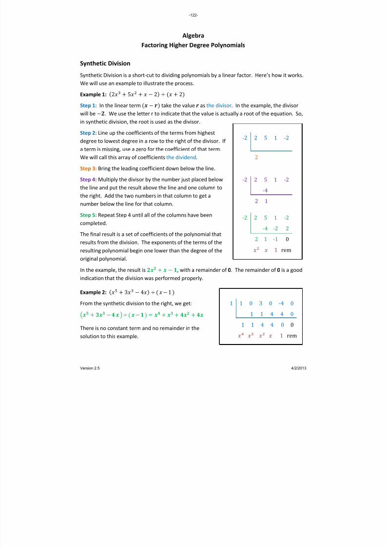
8/13/2019 AlgebraHandbook_very Helpful_ Print It
http://slidepdf.com/reader/full/algebrahandbookvery-helpful-print-it 122/178
Algebra Factoring Higher Degree Polynomials
Synthetic Division Synthetic
Division
is
a short
‐cut
to
dividing
polynomials
by
a linear
factor.
Here’s
how
it
works.
We will use an t ss. example o illustrate the proce
Example 1: 2 5 2
‐2 2 5 1 ‐2
2
‐2 2 5 1 ‐2‐4
2 1
‐2 2 5 1 ‐2‐4 ‐2 22 1 ‐1 0
1 rem
2 Step 1: In the linear term take the value r as the divisor. In the example, the divisor
will be . We use the letter r to indicate that the value is actually a root of the equation. So,
in synthetic division, the root is used as the divisor.
Step 2: Line up the coefficients of the terms from highest
degree to lowest degree in a row to the right of the divisor. If
a term
is
missing,
use
a zero
for
the
coefficient
of
that
term.
We will call this array of coefficients the dividend.
Step 3: Bring the leading coefficient down below the line.
Step 4: Multiply the divisor by the number just placed below
the line and put the result above the line and one column to
the right. Add the two numbers in that column to get a
number below the line for that column.
Step 5: Repeat Step 4 until all of the columns have been
completed.
The final result is a set of coefficients of the polynomial that
results from the division. The exponents of the terms of the
resulting polynomial begin one lower than the degree of the
original polynomial.
In the example, the result is , with a remainder of 0. The remainder of 0 is a good
indication th th d properly. at e division was performe
Example 2:
3
4 1
1 1 0 3 0 ‐4 01 1 4 4 0
1 1 4 4 0 0 1 rem
From the synthetic division to the we get:
right,
There is no constant term and no remainder in the
solution to this example.
-122-
Version 2.5 4/2/2013

8/13/2019 AlgebraHandbook_very Helpful_ Print It
http://slidepdf.com/reader/full/algebrahandbookvery-helpful-print-it 123/178
Algebra Comparing Synthetic Division to Long Division
Advantages of Synthetic Division Synthetic
division
has
the
following
advantages
over
long
division:
• The divisor is a possible root of the polynomial; it is a root if the remainder is zero.
• It is shorter.
• It is much quicker.
• It works by addition and multiplication instead of by subtraction and division. Because
of this, it is much less prone to error.
Comparison of Methods It
is
instructive
to
compare
synthetic
division
and
long
division
to
get
a better
idea
of
why
synthetic division works. Consider the division: 2 5 2 2
The two methods of performing this division are laid out below. Notice the following
correspondences between the examples:
• Root vs. Factor. Synthetic division uses the root of the
polynomial as the divisor. Long division uses the whole factor.
The signs on the root are opposite in the two methods.
Synthetic Division ‐2 2 5 1 ‐2
‐4 ‐2 2
2 1 ‐1 0
• Dividend. The dividends in the two methods are the same
(except that
synthetic
division
leaves
out
the
variables).
• Second Row. The second row in synthetic division
corresponds to the “secondary” coefficients of
each division in long division (but with opposite
signs). Long Division
2 1 1
2 1 2 2 5
2 4
2 1 2
1 2 1 2
0
• Answer Row. In synthetic division the answer row
(of coefficients) is calculated directly by adding the
values in the rows above it. In long division, it is
necessary to subtract expressions to determine
another expression
that
must
be
divided
by
the
divisor to get the next term of the answer.
• Adding Variables. In synthetic division, it is
necessary to add the variables after the answer is
determined. In long division, the answer is
provided directly.
-123-
Version 2.5 4/2/2013

8/13/2019 AlgebraHandbook_very Helpful_ Print It
http://slidepdf.com/reader/full/algebrahandbookvery-helpful-print-it 124/178
Algebra Zeroes of Polynomials
Developing Possible Roots
If a polynomial
has
the
form:
Then,
• will have exactly complex roots. For example, a 5th
degree polynomial will have
exactly 5 complex roots. Note: some of these roots may be the same, and some of
may be real. them
• will have exactly real roots, where is a whole number. For example, a
5th
degree polynomial will have either 5 real roots, 3 real roots, or 1 real root.
• Descartes’ Rule of Signs. (Note how this ties into the bull ve.) et abo
o The number of positive real roots of a polynomial is equal to the number of
sign changes in , or is less than this by a multip 2. le of
o The number of negative real roots of a polynomial is equal to the number
of sign changes in , or is less than this by a multiple of 2. Note: to
generate quickly, just change the signs of the terms with odd exponents.
• will have an even number of non‐real roots. For example, a 5th
degree polynomial
will have either 0
non‐real roots, 2
non‐real roots, or 4
non‐real roots. Further, the
non‐real roots exist in conjugate pairs; so if is a root of , then so is
.
• Rational Root Theorem. Any rational roots have the characteristic
. This
fact is especially useful if the lead coefficient of the polynomial is 1; in this case, any real
roots are factors of the constant term. This fact, in combination with the ease of
synthetic division, makes finding integer roots a quick process.
Example: What can we say about ? (note: 4 sign changes) the roots of
• Firs e that (note: zero sign changes) t, not
• So, has 4 complex roots. 0, 2, or 4 of them are real; all real roots are positive.
• The real roots must be 1, 2, or 4 (the positive factors of the constant term 4).
• To find out more, we have to test the possible real root values.
-124-
Version 2.5 4/2/2013
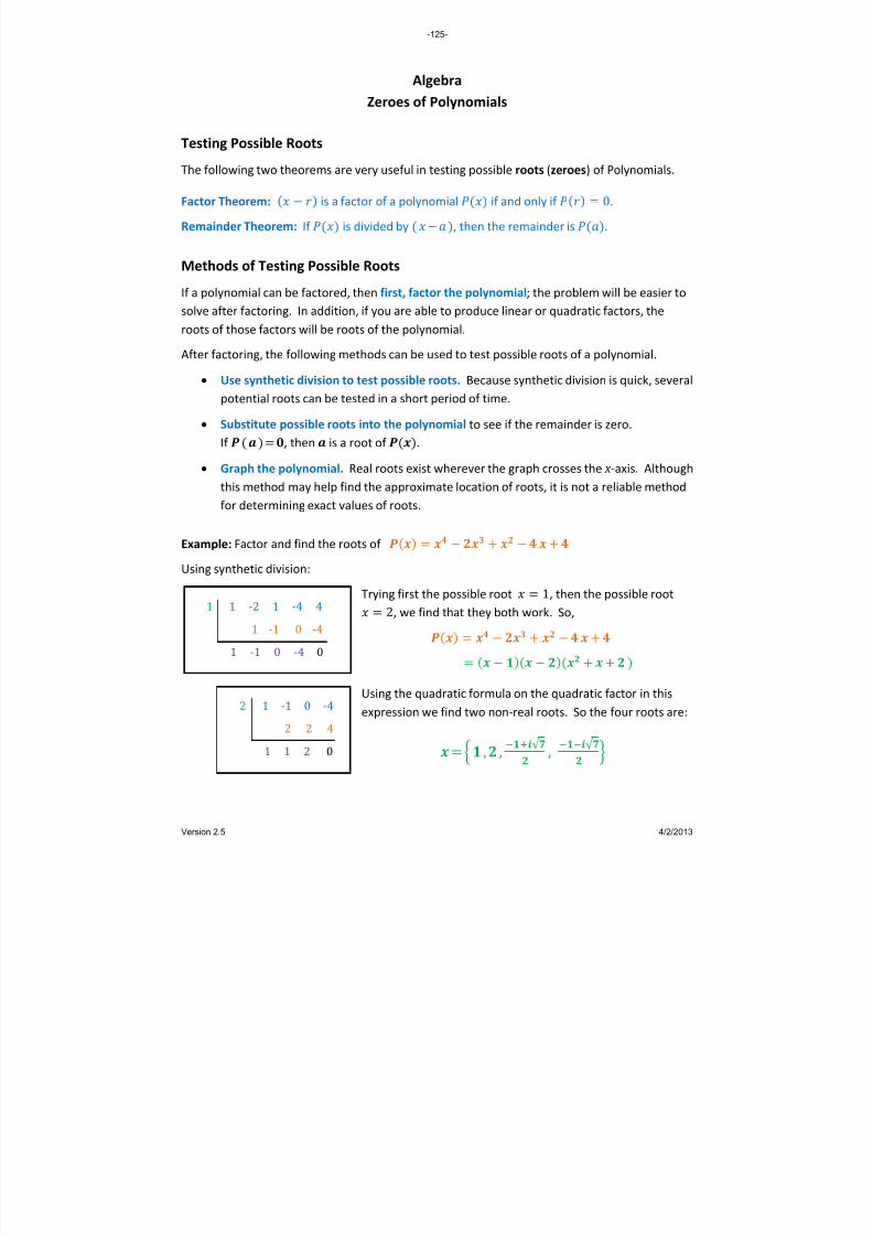
8/13/2019 AlgebraHandbook_very Helpful_ Print It
http://slidepdf.com/reader/full/algebrahandbookvery-helpful-print-it 125/178
Algebra Zeroes of Polynomials
Testing Possible Roots The
following
two
are
very
useful
in
testin sible
roots
(ze ) olynomials.
theorems g
pos roes
of
P
Factor Theorem: factor of a po l if and only if . is a lynomia 0Remainder Theorem: If is divided by , then the remainder is .
Methods of Testing Possible Roots If a polynomial can be factored, then first, factor the polynomial; the problem will be easier to
solve after factoring. In addition, if you are able to produce linear or quadratic factors, the
roots
of
those
factors
will
be
roots
of
the
polynomial.
After factoring, the following methods can be used to test possible roots of a polynomial.
• Use synthetic division to test possible roots. Because synthetic division is quick, several
potential roots can be tested in a short period of time.
• Substitute roots into t lynomial to see if the remainder is zero. possible he po
If , then is a root of .
• Graph the polynomial. Real roots exist wherever the graph crosses the x ‐axis. Although
this method may help find the approximate location of roots, it is not a reliable method
for determining
exact
values
of
roots.
1 1 ‐2 1 ‐4 4 1 ‐1 0 ‐4
1 ‐1 0 ‐4 0
Example: Factor and find the roots of
Trying first the possible root 1, then the possible root
Using synthetic division:
2, we find that they both work. So,
2 1 ‐1 0 ‐4 2 2 4
1 1 2 0
Using the quadratic formula on the quadratic factor in this
expression we ‐real roots. So th four roots are: find two non e
, , √ , √
-125-
Version 2.5 4/2/2013
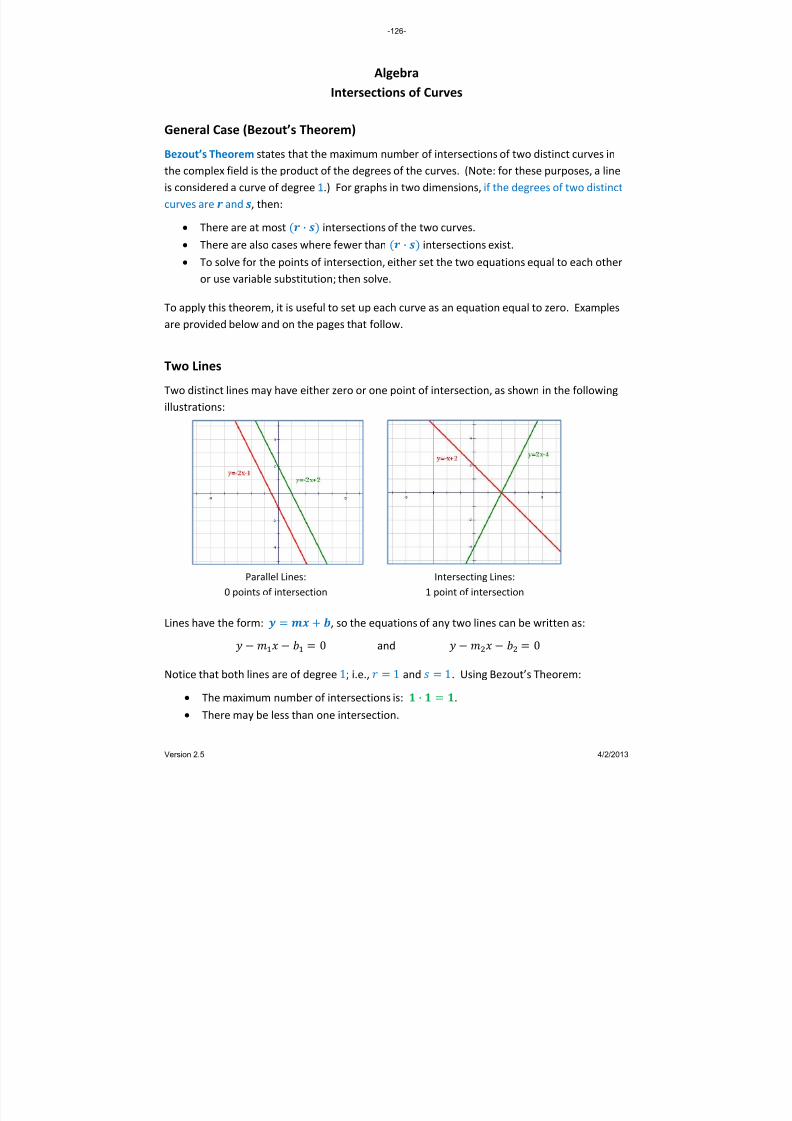
8/13/2019 AlgebraHandbook_very Helpful_ Print It
http://slidepdf.com/reader/full/algebrahandbookvery-helpful-print-it 126/178
Algebra Intersections of Curves
General Case (Bezout’s Theorem) Bezout’s Theorem states that the maximum number of intersections of two distinct curves in the complex field is the product of the degrees of the curves. (Note: for these purposes, a line is considered a curve of degree 1.) For graphs in two dimensions, if the degrees of two distinct curves are r and s, then:
• There are at most · intersections of the two curves. • There are also cases where fewer than · intersections exist. • To solve for the points of intersection, either set the two equations equal to each other or use variable substitution; then solve.
To apply this theorem, it is useful to set up each curve as an equation equal to zero. Examples are provided below and on the pages that follow.
Two Lines Two distinct lines may have either zero or one point of intersection, as shown in the following illustrations:
Lines have the form: , so the equations of any two lines can be written as: 0 and 0
Notice that both lines are of degree 1; i.e., 1 and 1. Using Bezout’s Theorem: • The maximum number of intersections is: · . • There may be less than one intersection.
Parallel Lines: 0 points of intersection
Intersecting Lines: 1 point of intersection
-126-
Version 2.5 4/2/2013

8/13/2019 AlgebraHandbook_very Helpful_ Print It
http://slidepdf.com/reader/full/algebrahandbookvery-helpful-print-it 127/178
Algebra Intersections of Curves
A Line and a Parabola The general forms for a line and a parabola are:
• Line: • Parabola:
For purposes of Bezout’s Theorem, these convert to: • Line: • Parabola:
Using Bezout’s Theorem, the maximum number of intersections is: · . Cases for 0, 1, and 2 intersections are provided below:
Finding the Point(s) of Intersection In order to find any points of intersection, set the two original equations equal to each other and solve:
This equation can be solved for x by any of the methods used to find the roots of a quadratic equation. The value of y can be calculated for each value of x by substituting x into either of the original equations.
Note: we use the letter “t” instead of “b” in the equation of a line in order to avoid confusion with the coefficient “b” in the equation of a parabola.
0 points of intersection 1 point of intersection 2 points of intersection
-127-
Version 2.5 4/2/2013

8/13/2019 AlgebraHandbook_very Helpful_ Print It
http://slidepdf.com/reader/full/algebrahandbookvery-helpful-print-it 128/178
Algebra Intersections of Curves
A Circle and an Ellipse The general forms for a circle and an ellipse are:
• Circle: • Ellipse:
For purposes of Bezout’s Theorem, these convert to: • Circle: • Ellipse:
Using Bezout’s Theorem, the maximum number of intersections is: · . Cases for 0, 1, 2, 3 and 4 intersections are provided below:
0 points of intersection 1 point of intersection 2 points of intersection
4 points of intersection 3 points of intersection
-128-
Version 2.5 4/2/2013

8/13/2019 AlgebraHandbook_very Helpful_ Print It
http://slidepdf.com/reader/full/algebrahandbookvery-helpful-print-it 129/178
Algebra
Domains of Rational Functions
Rational Expressions are fractions with polynomials in both the numerator and denominator. If
the rational
expression
is
a function,
it
is
a Rational
Function.
Finding the Domain of a Rational Function
The domain (e.g., x ‐values) of a rational function is the set of all values that result in valid range
values (e.g., y ‐values). Generally, there are two situations where a value is not included in the
domain of a rational function:
When the domain value results in a range value with zero in the denominator.
When the domain value results in a range value containing the square root of a negative
number.
Example 1:
Consider the rational function: .
Since there are no square roots, the only value for which
we cannot calculate is where or, where
. So the domain is all real x except , or:
|
Notice the hole in the graph of the function. This
indicates that the function does not have a value for
.
Example 2:
Consider the function:
This function has no valid x ‐values for 3 because
they would generate the square root of a negative
number in the numerator. In addition, the denominator
would be zero if . So the domain is all real x
greater than ‐3 except , or:
| 3
-129-
Version 2.5 4/2/2013

8/13/2019 AlgebraHandbook_very Helpful_ Print It
http://slidepdf.com/reader/full/algebrahandbookvery-helpful-print-it 130/178
Algebra
Holes and Asymptotes
Holes
A hole in a graph exists whenever a factor is in both
the numerator and denominator of a rational function, as
long as there is no vertical asymptote at .
Example: In the function the factor is
in both the numerator and the denominator. In fact, the
function can be reduced to except at the point
where the function is undefined.
Vertical Asymptotes
A vertical asymptote exists whenever a factor is in the denominator but not in the
numerator of a rational function.
Example: In the function
the factors
and are in the denominator but not in the
numerator of the function. The location of the vertical
asymptotes are shown as red dotted lines at and
in the
graph
at
right.
Horizontal Asymptotes
There are three separate cases for horizontal asymptotes of a rational function
:
1. If the degree of P(x) > the degree of Q(x), there is no horizontal asymptote.
2. If the degree of P(x) = the degree of Q(x), a horizontal asymptote exists at the line:
.
3. If the degree of P(x) < the degree of Q(x), a horizontal asymptote exists at the line .
Example: In the function
the degrees of the polynomials in the numerator
and denominator are the same, and the ratio of their lead coefficients is
. The location of
the horizontal asymptote is shown as the red dotted line in the graph above.
-130-
Version 2.5 4/2/2013
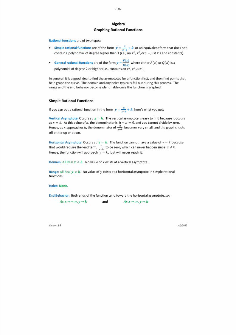
8/13/2019 AlgebraHandbook_very Helpful_ Print It
http://slidepdf.com/reader/full/algebrahandbookvery-helpful-print-it 131/178
Algebra
Graphing Rational Functions
Rational functions are of two types:
Simple rational functions are of the form
or an equivalent form that does not
contain a polynomial of degree higher than 1 (i.e., no , ,. – just ’s and constants).
General rational functions are of the form
where either or is a
polynomial of degree 2 or higher (i.e., contains an , ,.).
In general, it is a good idea to find the asymptotes for a function first, and then find points that
help graph the curve. The domain and any holes typically fall out during this process. The
range and the end behavior become identifiable once the function is graphed.
Simple Rational Functions
If you can put a rational function in the form
, here’s what you get:
Vertical Asymptote: Occurs at . The vertical asymptote is easy to find because it occurs
at . At this value of , the denominator is 0, and you cannot divide by zero.
Hence, as approaches , the denominator of
becomes very small, and the graph shoots
off either up or down.
Horizontal Asymptote: Occurs at . The function cannot have a value of because
that would require the lead term,
to be zero, which can never happen since 0.
Hence, the function will approach , but will never reach it.
Domain: All Real . No value of exists at a vertical asymptote.
Range: All Real . No value of exists at a horizontal asymptote in simple rational
functions.
Holes: None.
End Behavior: Both ends of the function tend toward the horizontal asymptote, so:
→∞,
→ and
→ ∞ ,
→
-131-
Version 2.5 4/2/2013
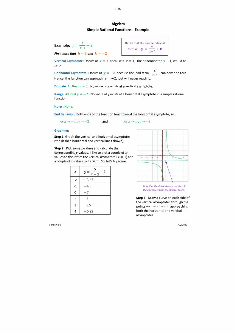
8/13/2019 AlgebraHandbook_very Helpful_ Print It
http://slidepdf.com/reader/full/algebrahandbookvery-helpful-print-it 132/178
Algebra
Simple Rational Functions ‐ Example
Example:
2
First, note that and Vertical Asymptote: Occurs at 1 because if 1, the denominator, 1, would be
zero.
Horizontal Asymptote: Occurs at 2 because the lead term,
, can never be zero.
Hence, the function can approach 2, but will never reach it.
Domain: All Real 1. No value of exists at a vertical asymptote.
Range: All Real 2. No value of y exists at a horizontal asymptote in a simple rational
function.
Holes: None.
End Behavior: Both ends of the function tend toward the horizontal asymptote, so:
→∞,
→ 2 and
→ ∞ ,
→ 2
Graphing:
Step 1.
Graph
the
vertical
and
horizontal
asymptotes
(the dashed horizontal and vertical lines shown).
Step 2. Pick some x‐values and calculate the
corresponding y ‐values. I like to pick a couple of ‐
values to the left of the vertical asymptote ( 1) and
a couple of x ‐values to its right. So, let’s try some.
x
‐2 3.67
‐1 4.5
0 7
2 3
3 0.5
4 0.33
Step 3. Draw a curve on each side of
the vertical asymptote: through the
points on that side and approaching
both the horizontal and vertical
asymptotes.
Note that the dot at the intersection of the asymptotes has coordinates ,.
Recall that the simple rational
form is:
-132-
Version 2.5 4/2/2013
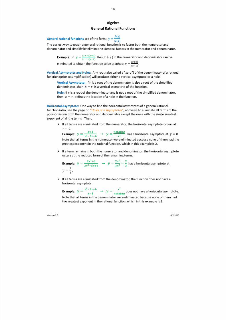
8/13/2019 AlgebraHandbook_very Helpful_ Print It
http://slidepdf.com/reader/full/algebrahandbookvery-helpful-print-it 133/178
Algebra
General Rational Functions
General rational functions are of the form:
The easiest
way
to
graph
a general
rational
function
is
to
factor
both
the
numerator
and
denominator and simplify by eliminating identical factors in the numerator and denominator.
Example: in
the 2 in the numerator and denominator can be
eliminated to obtain the function to be graphed:
.
Vertical Asymptotes and Holes: Any root (also called a “zero”) of the denominator of a rational
function (prior to simplification) will produce either a vertical asymptote or a hole.
Vertical Asymptote: If is a root of the denominator is also a root of the simplified
denominator, then
is
a vertical
asymptote
of
the
function.
Hole: If is a root of the denominator and is not a root of the simplified denominator,
then defines the location of a hole in the function.
Horizontal Asymptote: One way to find the horizontal asymptotes of a general rational
function (also, see the page on “Holes and Asymptotes” , above) is to eliminate all terms of the
polynomials in both the numerator and denominator except the ones with the single greatest
exponent of all the terms. Then,
If all terms are eliminated from the numerator, the horizontal asymptote occurs at
0.
Example:
→ has a horizontal asymptote at 0.
Note that all terms in the numerator were eliminated because none of them had the
greatest exponent in the rational function, which in this example is 2.
If a term remains in both the numerator and denominator, the horizontal asymptote
occurs at the reduced form of the remaining terms.
Example:
→
has a horizontal asymptote at
.
If all terms are eliminated from the denominator, the function does not have a
horizontal asymptote.
Example:
→
does not have a horizontal asymptote.
Note that all terms in the denominator were eliminated because none of them had
the greatest exponent in the rational function, which in this example is 2.
-133-
Version 2.5 4/2/2013

8/13/2019 AlgebraHandbook_very Helpful_ Print It
http://slidepdf.com/reader/full/algebrahandbookvery-helpful-print-it 134/178
Algebra
General Rational Functions (cont’d)
Domain: The domain is always “all Real ” except where there is a vertical asymptote or a hole.
No function
value
is
associated
with
at
either
a vertical
asymptote
or
a hole
(or
when
an
even
root of a negative number is required).
Range: The range is a bit trickier. You will need to look at the graph to determine the range.
You might think that no ‐value would exist at a horizontal asymptote, like in simple rational
functions. However, it is possible for a function to cross over its horizontal asymptote and then
work its way back to the asymptote as
→ ∞ or as
→ ∞. Odd but true (see below, right).
For oddities in the range of a function, check these out:
End Behavior: Both ends of the function tend toward the horizontal asymptote if there is one.
However, if there is not one, you must look at the graph to determine end behavior. Note that
the function below does not have a horizontal asymptote:
In this function,
→∞,
→ ∞,
→ ∞ ,
→ ∞
Although this function does not have a
horizontal asymptote, it does have a
non‐vertical asymptote: the line .
-134-
Version 2.5 4/2/2013
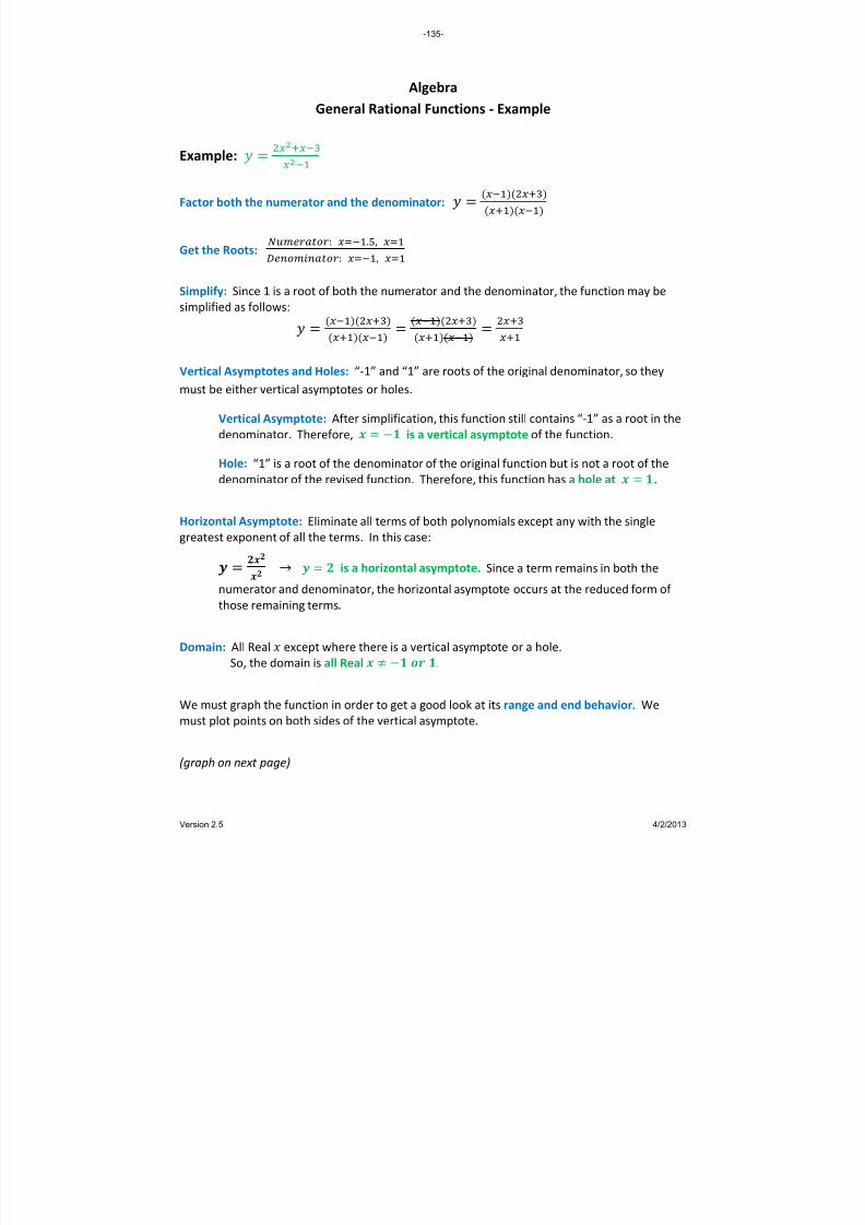
8/13/2019 AlgebraHandbook_very Helpful_ Print It
http://slidepdf.com/reader/full/algebrahandbookvery-helpful-print-it 135/178
Algebra
General Rational Functions ‐ Example
Example:
Factor both the numerator and the denominator:
Get the Roots: : ., : ,
Simplify: Since 1 is a root of both the numerator and the denominator, the function may be
simplified as follows:
Vertical Asymptotes and Holes: “‐1” and “1” are roots of the original denominator, so they
must be either vertical asymptotes or holes.
Vertical Asymptote: After simplification, this function still contains “‐1” as a root in the
denominator. Therefore, is a vertical asymptote of the function.
Hole: “1” is a root of the denominator of the original function but is not a root of the
denominator of the revised function. Therefore, this function has a hole at .
Horizontal Asymptote: Eliminate all terms of both polynomials except any with the single
greatest exponent of all the terms. In this case:
→ is a horizontal asymptote. Since a term remains in both the
numerator and denominator, the horizontal asymptote occurs at the reduced form of
those remaining terms.
Domain: All Real except where there is a vertical asymptote or a hole.
So, the
domain
is
all
Real
.
We must graph the function in order to get a good look at its range and end behavior. We
must plot points on both sides of the vertical asymptote.
(graph on next page)
-135-
Version 2.5 4/2/2013

8/13/2019 AlgebraHandbook_very Helpful_ Print It
http://slidepdf.com/reader/full/algebrahandbookvery-helpful-print-it 136/178
Step 3. Draw a curve on each side of the vertical asymptote:
through the points on that side and approaching both the
horizontal and vertical asymptotes.
Step 4:
Draw
an
open
circle
at
the
point
of
any
holes.
See the hole at ,.!
Algebra
General Rational Functions – Example (cont’d)
Graphing:
Step 1. Graph the vertical and horizontal asymptotes.
Step 2. Pick some ‐values on each side of the vertical asymptote and calculate the
corresponding y ‐values.
Range: The range must be determined from the graph.
It appears that the range excludes only the horizontal asymptote.
So the range is: all Real .
End Behavior:
In
this
function,
→∞,
→ ,
→ ∞ ,
→
x
‐4 1.67
‐3 1.5
‐2 1
0 3
1 2.5 (a hole)
2 2.33
-136-
Version 2.5 4/2/2013

8/13/2019 AlgebraHandbook_very Helpful_ Print It
http://slidepdf.com/reader/full/algebrahandbookvery-helpful-print-it 137/178
Algebra
Operating with Rational Expressions
Performing operations with rational expressions is very similar to performing operations with
fractions. After
all,
that’s
really
what
rational
expressions
are
–
fractions
involving
polynomials.
Addition and Subtraction
To add or subtract rational expressions:
Factor both the numerator and denominator as much as possible.
Create a common denominator.
Add or subtract expressions.
Simplify.
Example:
∙
∙
Multiplication
and
Division
To multiply or divide rational expressions:
Factor both the numerator and denominator as much as possible.
Multiply or divide expressions. (Remember, to divide, “flip that guy and multiply.”)
Cancel all factors that appear in both the numerator and denominator.
Simplify.
Example:
∙
∙
∙
Note that you can cross out common
factors in the numerator and
denominator across the expressions
that are
being
multiplied.
After the numerators are added, you must
check to see if the new numerator can be
factored. If
so,
further
simplification
may
be possible. Note: no further
simplification is possible in this example.
-137-
Version 2.5 4/2/2013

8/13/2019 AlgebraHandbook_very Helpful_ Print It
http://slidepdf.com/reader/full/algebrahandbookvery-helpful-print-it 138/178
Algebra
Solving Rational Equations
Solving Rational Equations
Solving rational equations involves one main rule: Get rid of the denominators!
A fuller listing of the steps involved is:
Multiply by whatever expressions are necessary to eliminate the denominators.
Pay careful attention to which values make the expressions you use equal to zero
(because you are not allowed to multiply both sides of an equation by zero).
Solve the remaining problem.
Check each answer to see if it is a solution to the original problem. Note: as long as you
do not multiply by zero, your solutions are likely to be valid.
Example 1: Solve
First note that x cannot be 3 or ‐1 since
each of these creates an undefined
fraction in the original problem.
The easiest way to start this problem is to
cross multiply to get:
1 3
Then, 2 1 6 9
So, 8 8
And finally,
Check work:
?
?
Example 2: Solve
First note that x cannot be ‐8 or ‐3 since
each of these creates an undefined
fraction in the original problem.
The easiest way to start this problem is to
cross multiply to get:
3 8
Then, 2 8 0
So, 4 2 0
And finally,
Check ‐4:
?
?
Check 2:
?
-138-
Version 2.5 4/2/2013

8/13/2019 AlgebraHandbook_very Helpful_ Print It
http://slidepdf.com/reader/full/algebrahandbookvery-helpful-print-it 139/178
Case 1: 0 1
Then: 3 5 2 2
So, 3
The solution here requires:
Which simplifies to: 3 1 3
Case 2: 0 1
Then: 3 5 2 2
So, 3
The solution here requires:
Which simplifies to: 1 1 3
Algebra
Solving Rational Inequalities
Solving Rational Inequalities
Solving Rational
Inequalities
is
a bit
more
involved
than
solving
Rational
Equations.
The
key
issue in the Inequalities is whether in the step where you eliminate the denominator, you are
multiplying by a negative number. Remember, when you multiply by a negative number, you
must flip an inequality sign.
The steps involved are similar to those for solving rational equations:
Multiply by whatever expressions are necessary to eliminate the denominators.
Identify when the denominators are positive and when they are negative; set up cases
for each situation. Within each case, you will need to meet multiple conditions (i.e.,
using the word “and” between conditions within a case).
Pay careful attention to which values make the expression you multiply equal to zero
(because you are not allowed to multiply both sides of an inequality by zero).
Solve the remaining problems. Any of the cases produces valid results, so you must
combine the solutions for the various cases with “or’s.”
Check sample answers in each range you develop to see if they are solutions to the
original problem. Alternatively, graph the solution to see if the results are correct.
Example: Solve
2
We want
to
eliminate
the
denominator
but
we
need
to
create
2 cases:
The combined result of the two cases is:
1 3
To check the result, we graph the function and see
where it produces a y ‐value above 2; this is the set
of x ‐values where the dark green curve intersects
the light green region in the graph below.
-139-
Version 2.5 4/2/2013
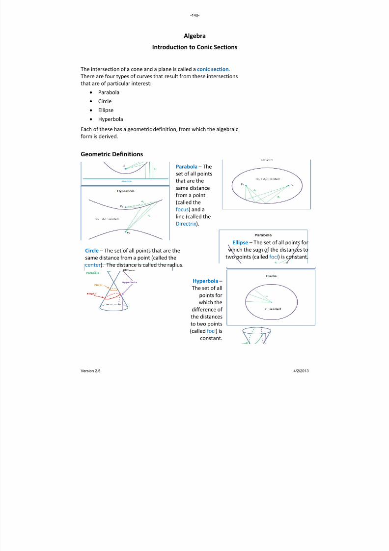
8/13/2019 AlgebraHandbook_very Helpful_ Print It
http://slidepdf.com/reader/full/algebrahandbookvery-helpful-print-it 140/178
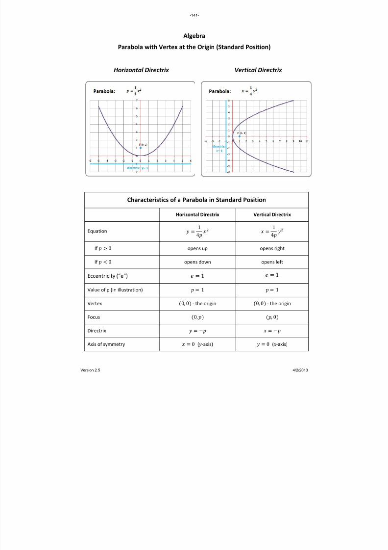
8/13/2019 AlgebraHandbook_very Helpful_ Print It
http://slidepdf.com/reader/full/algebrahandbookvery-helpful-print-it 141/178
Algebra Parabola with Vertex at the Origin (Standard Position)
Horizontal Directrix Vertical Directrix
Characteristics of a Parabola in Standard Position Horizontal Directrix Vertical Directrix
Equation 1
4
1
4
If 0 opens up opens right
If 0 opens down opens left
Eccentricity (“e”) 1 1
Value of p (in illustration) 1 1
Vertex 0, 0 ‐ the origin 0, 0 ‐ the origin
Focus 0, , 0
Directrix
Axis of symmetry 0 ( y ‐axis) 0 ( x ‐axis)
-141-
Version 2.5 4/2/2013

8/13/2019 AlgebraHandbook_very Helpful_ Print It
http://slidepdf.com/reader/full/algebrahandbookvery-helpful-print-it 142/178
Algebra Parabola with Vertex at ,
Horizontal Directrix Vertical Directrix
Characteristics of a Parabola with Vertex at Point , Horizontal Directrix Vertical Directrix
Equation 1
4
1
4
If 0 opens up opens right
If 0 opens down opens left
Eccentricity (“e”) 1 1
Vertex
,
,
Focus , ,
Directrix
Axis of symmetry
-142-
Version 2.5 4/2/2013
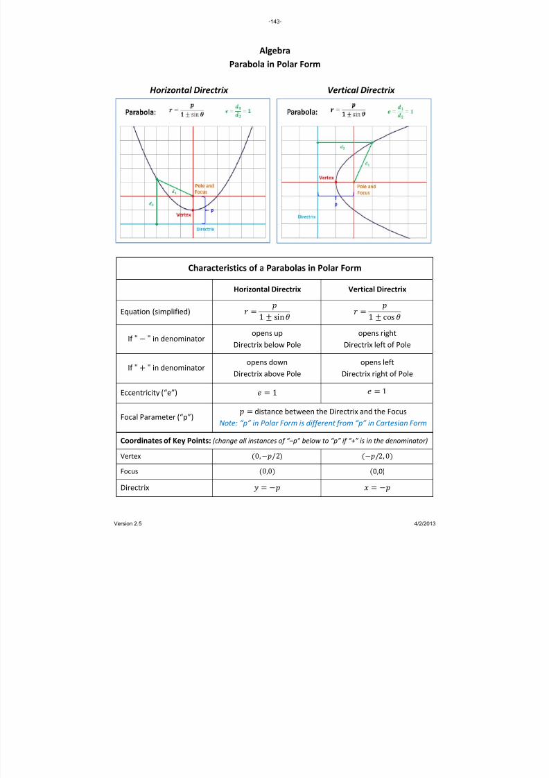
8/13/2019 AlgebraHandbook_very Helpful_ Print It
http://slidepdf.com/reader/full/algebrahandbookvery-helpful-print-it 143/178
Algebra Parabola in Polar Form
Horizontal Directrix Vertical Directrix
Characteristics of a Parabolas in Polar Form Horizontal Directrix Vertical Directrix
Equation (simplified)
1 sin
1 cos
If " " in denominator opens up
Directrix below Pole
opens right
Directrix left of Pole
If " " in denominator opens down
Directrix above Pole
opens left
Directrix right of Pole
Eccentricity (“e”) 1 1
Focal
Parameter
(“p”)
distance between the Directrix and the Focus
Note: “p” in Polar Form is different from “p” in Cartesian Form
Coordinates of Key Points: (change all instances of “–p” below to “p” if “+” is in the denominator) Vertex 0, /2 /2, 0
Focus 0,0 0,0)
Directrix
-143-
Version 2.5 4/2/2013

8/13/2019 AlgebraHandbook_very Helpful_ Print It
http://slidepdf.com/reader/full/algebrahandbookvery-helpful-print-it 144/178
Algebra Circles
Characteristics of a Circle in Standard Position
Equation
Center 0,0 ‐ the origin
Radius
In the example 4
Characteristics of a Circle in Polar Form
Equation
Pole 0, 0
Radius
Characteristics of a Circle Centered at Point (h, k)
Equation
Center ,
Radius
-144-
Version 2.5 4/2/2013

8/13/2019 AlgebraHandbook_very Helpful_ Print It
http://slidepdf.com/reader/full/algebrahandbookvery-helpful-print-it 145/178
Algebra Ellipse Centered on the Origin (Standard Position)
Vertical Major Axis Horizontal Major Axis
Characteristics of an Ellipse in Standard Position Horizontal Major Axis Vertical Major Axis
In the above example 5, 4, 3 5, 4, 3
Equation
1
1
Values of "" and ""
Value of ""
Eccentricity (“e”) / 0 1
Center 0,0 ‐ the origin
Major Axis Vertices , 0 0,
Minor Axis Vertices 0, , 0
Foci , 0 0,
Directrixes (not shown) / /
-145-
Version 2.5 4/2/2013
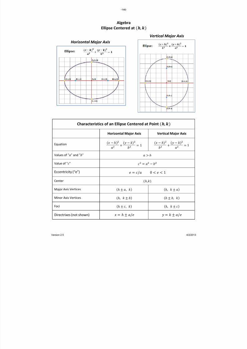
8/13/2019 AlgebraHandbook_very Helpful_ Print It
http://slidepdf.com/reader/full/algebrahandbookvery-helpful-print-it 146/178
Algebra Ellipse Centered at ,
Vertical Major Axis Horizontal Major Axis
Characteristics of an Ellipse Centered at Point , Horizontal Major Axis Vertical Major Axis
Equation
1
1
Values of "" and ""
Value of ""
Eccentricity (“e”) / 0 1
Center ,
Major Axis
Vertices
,
,
Minor Axis Vertices , ,
Foci , ,
Directrixes (not shown) / /
-146-
Version 2.5 4/2/2013
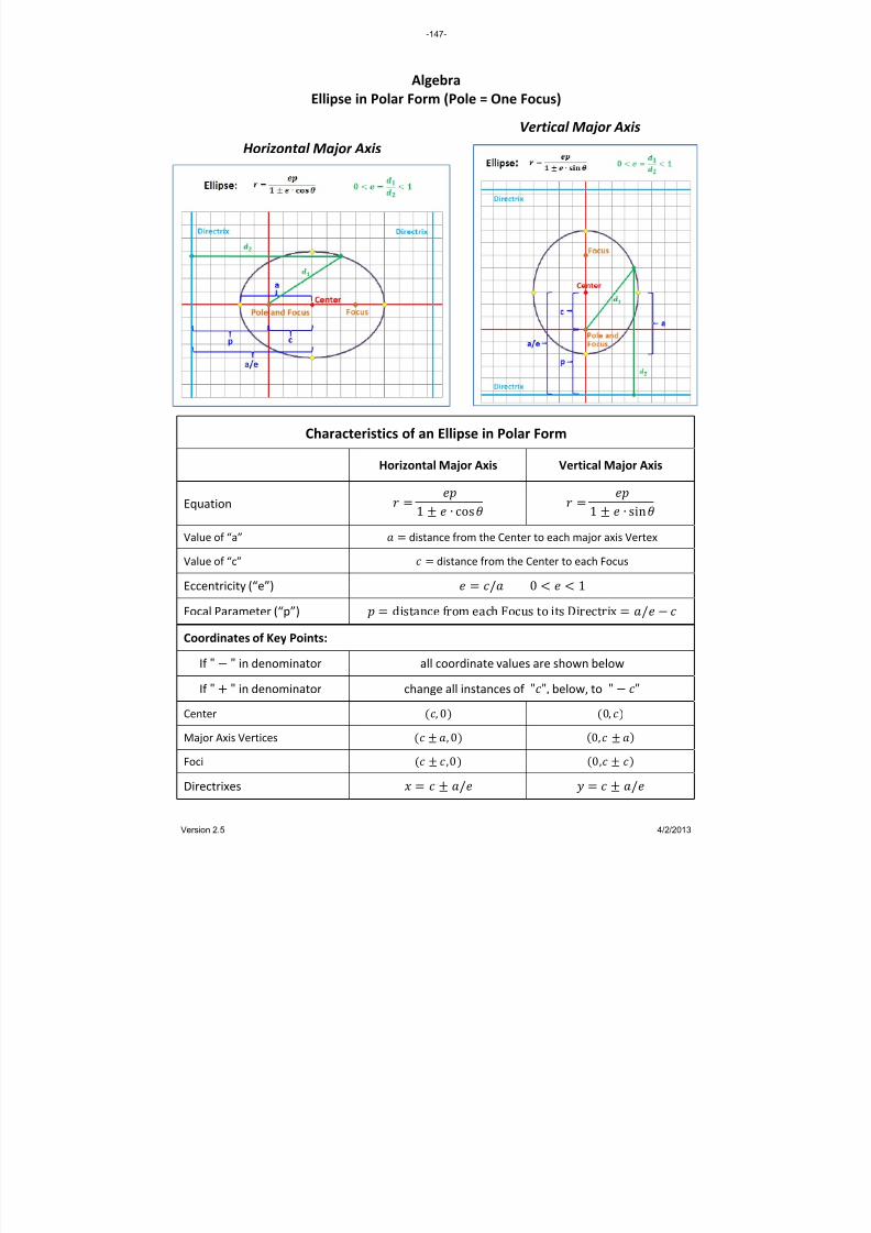
8/13/2019 AlgebraHandbook_very Helpful_ Print It
http://slidepdf.com/reader/full/algebrahandbookvery-helpful-print-it 147/178
Algebra Ellipse in Polar Form (Pole = One Focus)
Vertical Major Axis Horizontal Major Axis
Characteristics of an Ellipse in Polar Form Horizontal Major Axis Vertical Major Axis
Equation
1 ∙ cos
1 ∙ sin
Value of “a” distance from the Center to each major axis Vertex
Value of “c” distance from the Center to each Focus
Eccentricity (“e”) / 0 1
Focal Parameter (“p”) distance from each Focus to its Directrix /
Coordinates of Key Points: If
" "
in
denominator
all
coordinate
values
are
shown
below
If " " in denominator change all instances of "", below, to " "
Center , 0 0,
Major Axis Vertices , 0 0,
Foci ,0 0,
Directrixes / /
-147-
Version 2.5 4/2/2013

8/13/2019 AlgebraHandbook_very Helpful_ Print It
http://slidepdf.com/reader/full/algebrahandbookvery-helpful-print-it 148/178
Algebra Hyperbola Centered on the Origin (Standard Position)
Horizontal Transverse Axis Vertical Transverse Axis
Characteristics of a Hyperbola in Standard Position Horizontal Transverse Axis Vertical Transverse Axis
In the above example 3, 4, 5 4, 3, 5
Equation
1
1
Value of “c”
Eccentricity (“e”) / 1
Center 0,0 ‐ the origin
Vertices , 0 0,
Foci , 0 0,
Asymptotes
Directrixes (not shown) / /
-148-
Version 2.5 4/2/2013

8/13/2019 AlgebraHandbook_very Helpful_ Print It
http://slidepdf.com/reader/full/algebrahandbookvery-helpful-print-it 149/178
Algebra Hyperbola Centered at ,
Horizontal Transverse Axis Vertical Transverse Axis
Characteristics of a Hyperbola Centered at Point , Horizontal Transverse Axis Vertical Transverse Axis
Equation
1
1
Value of “c”
Eccentricity (“e”) / 1
Center ,
Vertices , ,
Foci , ,
Asymptotes
Directrixes (not shown) / /
-149-
Version 2.5 4/2/2013

8/13/2019 AlgebraHandbook_very Helpful_ Print It
http://slidepdf.com/reader/full/algebrahandbookvery-helpful-print-it 150/178
Algebra Hyperbola in Polar Form (Pole = One Focus)
Horizontal Transverse Axis Vertical Transverse Axis
Characteristics of a Hyperbola in Polar Form Horizontal Transverse Axis Vertical Transverse Axis
Equation
1 ∙ cos
1 ∙ sin
Value of “a” distance from the Center to each Vertex
Value of “c” distance from the Center to each Focus
Eccentricity (“e”) / 1
Focal Parameter (“p”) distance from each Focus to its Directrix /
Coordinates of Key Points: If " " in denominator all coordinate values are shown below
If " "
in
denominator
change all instances of "– ", below, to ""
Center , 0 0,
Vertices , 0 0,
Foci , 0 0,
Directrixes / /
-150-
Version 2.5 4/2/2013

8/13/2019 AlgebraHandbook_very Helpful_ Print It
http://slidepdf.com/reader/full/algebrahandbookvery-helpful-print-it 151/178
Algebra Hyperbola in Polar Form (Pole = One Focus)
Partial Construction Over the Domain: to It is instructive to look at partial constructions of a hyperbola in polar form. Let’s take a look at
a curve constructed by varying from 0 to 2, quadrant by quadrant:
:
: , , ,
In the plots below, each quadrant in the domain is represented by a separate color. The
portion of the curve added in each illustration is presented as a thicker line than the rest of the
curve. The Foci of the curve are dark blue points and the Directrixes are light blue vertical lines.
The final curve looks like this.
The curve is plotted over the
domain 0 2
but
could
also be plotted over the domain
.
The cosine function has a major
impact on how the curve graphs.
Note the
two
yellow
points
where cos 0.5. At these
points, the curve is undefined.
Q I: Domain 0 /2. Note
that the curve starts out on the
left and
switches
to
the
right
at
/3, where the curve is
undefined.
Q II: Domain /2 . The
curve continues on the right side
of the graph and gently curves
down to the x‐axis.
Q III: Domain 3/2.
The curve continues its gentle
swing below the x‐axis. Q III is
essentially a reflection of the
curve in Q II over the x‐axis.
Q IV: Domain 3/2 2.
The curve continues on the right
and switches to the left at
5/3, where the curve is
undefined.
-151-
Version 2.5 4/2/2013

8/13/2019 AlgebraHandbook_very Helpful_ Print It
http://slidepdf.com/reader/full/algebrahandbookvery-helpful-print-it 152/178
Examples: 3 2 4 0
2 7 1 0
3 2 7 3 0
4 2 1 0
4 9 8 27 2 0
3 6 12 15 0
4 10 0
4
4
16 8 5 0
5 3 20 12 3 0
2 8 12 13 0
Algebra General Conic Equation – Classification
The General Case of the Conic Equation is:
The second term may be omitted if the curve is not rotated relative to the axes in the Cartesian
Plane, giving the simpler form:
Conic Classification Tree In this form, it is relatively easy to identify which type of curve the equation represents, using
the following decision tree:
no
no
no
yes
no
yes
0
Are and
both missing?
The equation is not
a conic. It is a line.
Are and
different numbers?
( )
Are and the
same number?
∙ 0
Are the signs on
and
different?
∙ 0
Is either or
missing?
The equation is a
parabola.
The equation is a
hyperbola.
The equation is a
circle.
The equation is an
ellipse.
yes
yes
yes
-152-
Version 2.5 4/2/2013
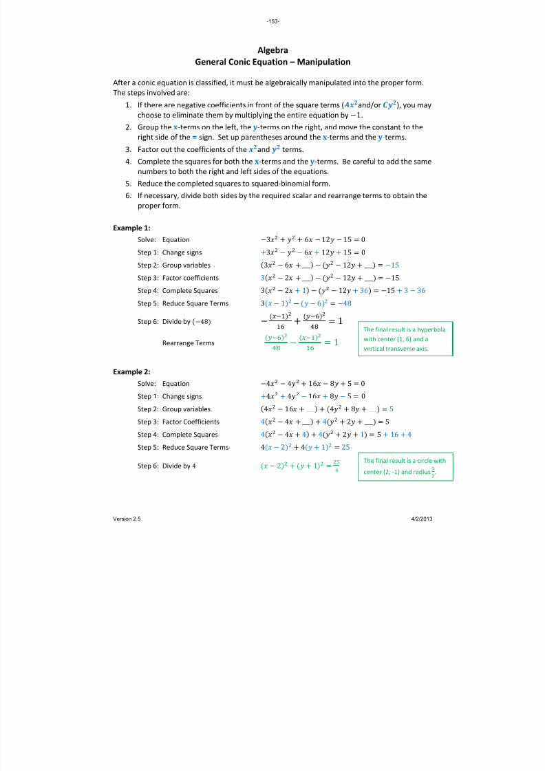
8/13/2019 AlgebraHandbook_very Helpful_ Print It
http://slidepdf.com/reader/full/algebrahandbookvery-helpful-print-it 153/178
Algebra General Conic Equation – Manipulation
After a conic equation is classified, it must be algebraically manipulated into the proper form.
The steps involved are:
1. If there
are
negative
coefficients
in
front
of
the
square
terms
( and/or
),
you
may
choose to eliminate them by multiplying the entire equation by 1.
2. Group the x‐terms on the left, the y‐terms on the right, and move the constant to the
right side of the = sign. Set up parentheses around the x‐terms and the y‐terms.
3. Factor out the coefficients of the and terms.
4. Complete the squares for both the x‐terms and the y‐terms. Be careful to add the same
numbers to both the right and left sides of the equations.
5. Reduce the completed squares to squared‐binomial form.
6. If necessary, divide both sides by the required scalar and rearrange terms to obtain the
proper
form.
Example 1: Solve: Equation 3 6 12 15 0
Step 1: Change signs 3 6 12 15 0
Step 2: Group variables 3 6 ___ 12 ___ 15
Step 3: Factor coefficients 3 2 ___ 12 ___ 15
Step 4: Complete Squares 3 2 1 12 36 15 3 36
Step 5: Reduce Square Terms 3 1 6 48
Step 6: Divide by 48
1
Rearrange Terms
1
Example 2: Solve: Equation 4 4 16 8 5 0
Step 1: Change signs 4 4 16 8 5 0
Step 2: Group variables 4 16 ___ 4 8 ___ 5
Step 3: Factor Coefficients 4 4 ___ 4 2 ___ 5
Step 4: Complete Squares 4 4 4 4 2 1 5 16 4
Step 5: Reduce Square Terms 4 2 4 1 25
Step 6: Divide by 4 2 1
The final result is a hyperbola
with center (1, 6) and a
vertical transverse axis.
The final result is a circle with
center (2, ‐1) and radius
.
-153-
Version 2.5 4/2/2013

8/13/2019 AlgebraHandbook_very Helpful_ Print It
http://slidepdf.com/reader/full/algebrahandbookvery-helpful-print-it 154/178
ADVANCED Algebra
Parametric Equations of Conic Sections Parabola (note: 4 1
Parametric Equations Centered at the Origin
Parametric Equations Centered at (h, k)
Circle Parametric Equations Centered at the Origin
Parametric Equations Centered at (h, k)
∙ ∙
∙ ∙
Ellipse Parametric Equations Centered at the Origin Parametric Equations
Centered at (h, k) ∙ ∙
∙ ∙
Hyperbola Parametric Equations Centered at the Origin
Parametric Equations Centered at (h, k)
∙ ∙
∙ ∙
-154-
Version 2.5 4/2/2013

8/13/2019 AlgebraHandbook_very Helpful_ Print It
http://slidepdf.com/reader/full/algebrahandbookvery-helpful-print-it 155/178
Algebra
Introduction to Sequences and Series
Definitions
• A Sequence
is
an
ordered
set
of
numbers.
• A Term is an element in the set of ordered numbers.
• An Infinite Sequence has no end. A Finite Sequence has a final term.
• An Explicit Formula is one that specifically defines the terms of the sequence based on the
number of the term. By convention, the number of the term is usually expressed in terms
of the variables or . We talk of the nth term or the k th term of the sequence or series.
• A Recursive Formula defines a term based on one or more previous terms.
• A Series is an ordered summation of a sequence.
Example (Sequence
and
Series):
Consider the sequence defined by the explicit formula: 3 1 .
The notation refers to the nth term of the sequence. So, we can construct both a sequence
and a series from this. Here are the first seven terms of the sequence and the series:
n 1 2 3 4 5 6 7
4 7 10 13 16 19 22
Sum of
4 11 21 34 50 69 91
Example (Recursive Formula):
One of the simplest and most famous recursive formulas is the Fibonacci Sequence, defined as:
This simply means that each term is the sum of the two terms before it. The Fibonacci
Sequence begins with a pair of ones, and uses the recursive formula to obtain all other terms:
n
1
2
3
4
5
6
7 1 1 2 3 5 8 13
Sum of 1 2 4 7 12 20 33
This sequence has some very interesting properties, which will be discussed on another page.
-155-
Version 2.5 4/2/2013

8/13/2019 AlgebraHandbook_very Helpful_ Print It
http://slidepdf.com/reader/full/algebrahandbookvery-helpful-print-it 156/178
One way to express this result is:
ADVANCED
Algebra
The Fibonacci Sequence
The Fibonacci Sequence was first published in 1202 by Leonardo Fibonacci (of Pisa). It starts
with a pair of ones and continues with the recursive formula: . The beginning
of the sequence looks like this:
1,1,2,3,5,8,13,21,34,55,89,144,233,377,610,987,…
Properties of the Fibonacci Sequence
It is possible to spend a long time exploring the properties of this simple sequence. Here are a
few of the more interesting properties:
Illustration 1: Add the sequence to create a series.
n 1 2 3 4 5 6 7 8 9 10 1 1 2 3 5 8 13 21 34 55 1 2 4 7 12 20 33 54 88 143
Notice that : .
That is, the nth sum is one less than the term of the original sequence two positions further to
the right!
Illustration 2: Calculate the squares and add the resulting sequence to create a series.
n 1 2 3 4 5 6 7 8 9 10 1 1 2 3 5 8 13 21 34 55
1 1 4 9 25 64 169 441 1156 3025 1 2 6 15 40 104 273 714 1870 4895
Notice that : · . That is, the nth
sum of the squares is the product of the two terms from the original sequence,
one of which is in the same position and one of which is one position to the right!
The Golden
Ratio
(f )
Ratios of successive values of the Fibonacci Sequence approach the Golden Ratio: f √ .
1.6
1.625 1.615
1.619 …
The approximate value of f √ 1.618034 f
-156-
Version 2.5 4/2/2013

8/13/2019 AlgebraHandbook_very Helpful_ Print It
http://slidepdf.com/reader/full/algebrahandbookvery-helpful-print-it 157/178
Algebra
Summation Notation and Properties
Summation Notation
Mathematicians are
fond
of
finding
shorthand
ways
of
expressing
things,
so
they
invented
notation for the summation of numbers. If we consider the series for 3 1 , the
notation for the series would be:
3 1
This simply means that the nth term of the series is defined by adding the first n term of the
sequence for 3 1 .
Example:
n 1 2 3 4 5 6 7
4 7 10 13 16 19 22
4 11 21 34 50 69 91
Note that 4 7 10 21 .
Although it looks complicated at first, after you write a few series longhand, you will begin to
appreciate the
shorthand
notation.
Summation Properties
Here are a couple of useful properties of summations, all of which are based on the algebraic
properties of addition, multiplication and equality. and are two series. c and d are real.
You can factor a constant out of a
summation if is a factor of all the terms.
The sum of two series can be broken out
into the summations for each series.
· ·
· · ·
·
This is basically the distributive property of
multiplication over addition.
-157-
Version 2.5 4/2/2013
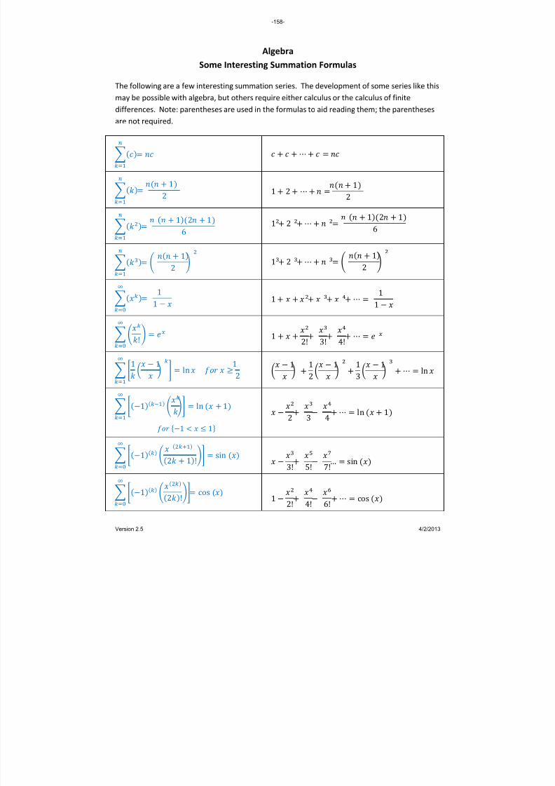
8/13/2019 AlgebraHandbook_very Helpful_ Print It
http://slidepdf.com/reader/full/algebrahandbookvery-helpful-print-it 158/178
Algebra
Some Interesting Summation Formulas
The following are a few interesting summation series. The development of some series like this
may be possible with algebra, but others require either calculus or the calculus of finite
differences.
Note: parentheses
are
used
in
the
formulas
to
aid
reading
them;
the
parentheses
are not required.
12
1 2 12
12 16
1 2 12 16
12
1 2 12
11
1 11
!
1 2! 3! 4!
1 1
ln 12 1 12 1
13 1 ln
1 ln 1
1 1
2
3
4 ln 1
1 2 1! sin
3! 5! 7! … sin
1 2! cos
1 2! 4! 6! cos
-158-
Version 2.5 4/2/2013

8/13/2019 AlgebraHandbook_very Helpful_ Print It
http://slidepdf.com/reader/full/algebrahandbookvery-helpful-print-it 159/178
These two equations
are equivalent.
Algebra
Arithmetic Sequences
An Arithmetic Sequence is one in which the terms are separated by a constant. The constant,
often indicated by the letter d , is called the Common Difference. Arithmetic sequences, then
meet the condition:
, where d is the common difference.
Example:
n 1 2 3 4 5 6 9 12 15 18 21 24
First Differences 3 3 3 3 3
In this sequence, the common difference is 3. If there is not a common difference, the
sequence is not arithmetic.
nth Term of an Arithmetic Sequence
The formula for the nth term of an arithmetic sequence is:
·
The problem with this formula is the
that gets multiplied by d . Sometimes this is hard
to remember.
An
alternative
method
would
be
to
first
calculate
a term
zero,
Then: · , which seems a nicer formula
The value of this alternative is that it also allows the student to establish a formula in form for the sequence, where is the y‐intercept, and , the common difference,
is the slope.
Example: In the above example, the nth term of the sequence can be written:
·
Or, first calculate:
Then: or
Either method works; the student should use whichever one they find more comfortable.
-159-
Version 2.5 4/2/2013
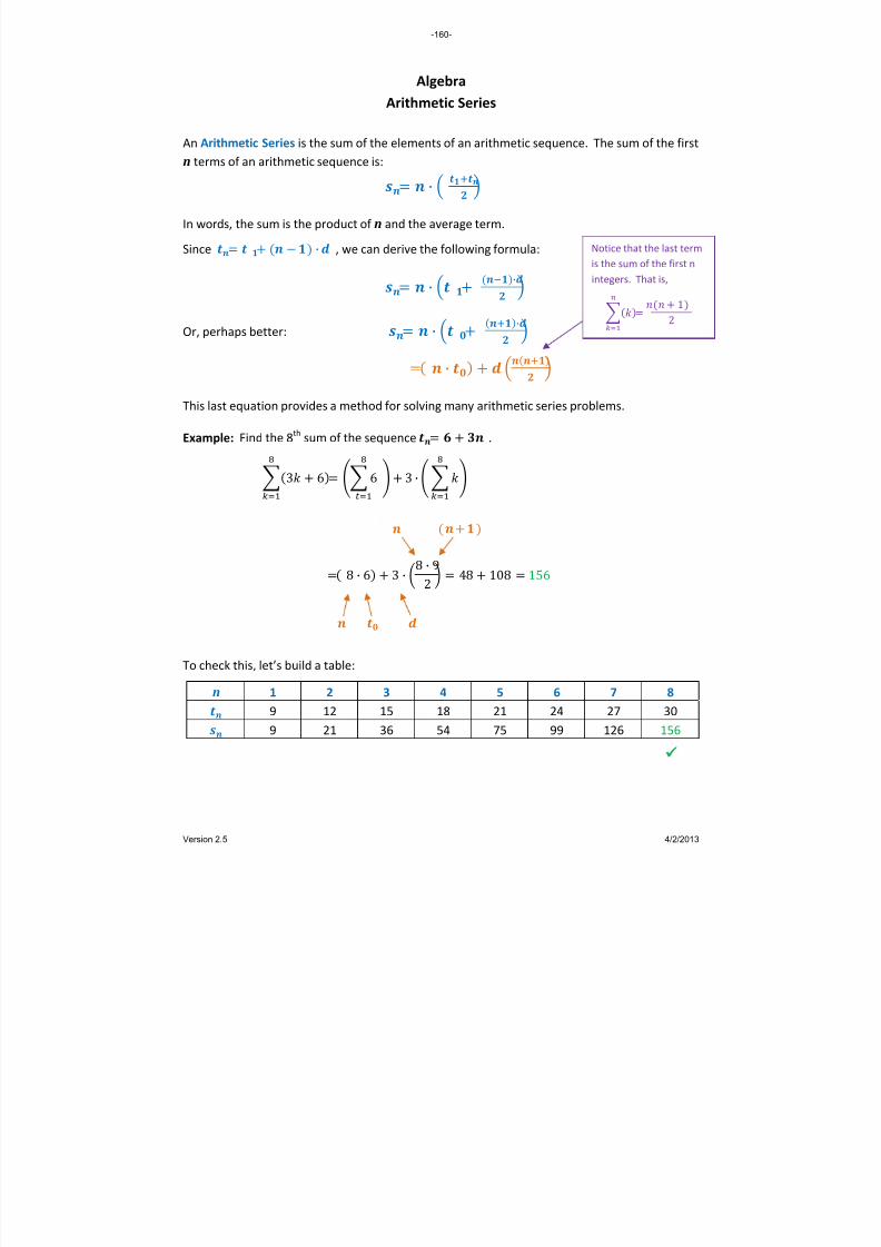
8/13/2019 AlgebraHandbook_very Helpful_ Print It
http://slidepdf.com/reader/full/algebrahandbookvery-helpful-print-it 160/178
Algebra
Arithmetic Series
An Arithmetic Series is the sum of the elements of an arithmetic sequence. The sum of the first
n terms of an arithmetic sequence is:
·
In words, the sum is the product of n and the average term.
Since · , we can derive the following formula:
· ·
Or,
perhaps
better:
· ·
·
This last equation provides a method for solving many arithmetic series problems.
Example: Find the 8th
sum of the sequence .
3 6 6
3 ·
8 · 6 3 · 8 · 92 48 108 156
To check this, let’s build a table:
n 1 2 3 4 5 6 7 8 9 12 15 18 21 24 27 30 9 21 36 54 75 99 126 156
12
Notice that the last term
is the sum of the first n
integers. That is,
-160-
Version 2.5 4/2/2013

8/13/2019 AlgebraHandbook_very Helpful_ Print It
http://slidepdf.com/reader/full/algebrahandbookvery-helpful-print-it 161/178
Algebra
Pythagorean Means
Consider a set of n values. We can take a mean of these n values in several ways. The three
classical methods of calculating a mean are called Pythagorean Means.
Arithmetic Mean
The arithmetic mean is the one that students are most familiar with. It is also called the
average. It is simply the sum of the n items, divided by n.
…
Example: Calculate the arithmetic mean of 5 test scores: 92, 94, 85, 72, 99
92948674995 89
Trick: A shortcut to calculating an arithmetic mean:
• Estimate a value for the average by “eyeballing” the values. For
the example above, it looks like 90 would be a good estimate.
• Subtract the estimate from each value to get a set of n
differences.
• Add the n differences and divide by n.
• Add the result to the original estimate. The result is the
arithmetic mean of the original set of values. In the above
example, the result is: 90 1 89 .
Geometric Mean
The geometric mean is the n‐th root of the product of the n values.
…
Example: Calculate the geometric mean of 2, 9, and 12:
√ 2 9 1 2 √ 216 6
Trick Example:
Score Value vs. 90
92 +2
94 +4
86 ‐4
74 ‐
16
99 +9
Total ‐5
Average ‐1
-161-
Version 2.5 4/2/2013

8/13/2019 AlgebraHandbook_very Helpful_ Print It
http://slidepdf.com/reader/full/algebrahandbookvery-helpful-print-it 162/178
Algebra
Pythagorean Means (cont’d)
Harmonic Mean
The harmonic
mean
is
reciprocal
of
the
arithmetic
mean
of
the
reciprocals
of
the n
values.
It
has applications in science.
1 · 1 11 · 1 1 1
Example:
Since the
harmonic
mean
looks
so
odd,
it
is
useful
to
look
at
a real
‐life
example.
Consider a car that travels 15 miles at 30 miles per hour, then another 15 miles at 15 miles per
hour. The average speed of the car over this distance is generated by the harmonic mean.
First, calculate the average speed from basic principles:
• 15 miles at 30 miles per hour takes 30 minutes.
• 15 miles at 15 miles per hour takes 60 minutes.
• Total trip is 30 miles in 90 minutes, for an average speed of 20 miles per hour.
Now, calculate the harmonic mean of the two speeds:
2 130 115 2 330 603 20
Comparing Means
Compare the values of the three Pythagorean Means of 3, 6, and 12:
:arithmetic mean
: geometic mean √ 3 6 1 2
:harmonic mean
In general, it is true that:
However, if the values being
averaged are all the same,
-162-
Version 2.5 4/2/2013
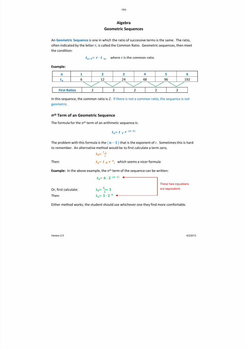
8/13/2019 AlgebraHandbook_very Helpful_ Print It
http://slidepdf.com/reader/full/algebrahandbookvery-helpful-print-it 163/178
These two equations
are equivalent.
Algebra
Geometric Sequences
An Geometric Sequence is one in which the ratio of successive terms is the same. The ratio,
often indicated by the letter r , is called the Common Ratio. Geometric sequences, then meet
the condition:
· , where r is the common ratio.
Example:
n 1 2 3 4 5 6 6 12 24 48 96 192
First Ratios 2 2 2 2 2
In this sequence, the common ratio is 2. If there is not a common ratio, the sequence is not
geometric.
nth Term of an Geometric Sequence
The formula for the nth term of an arithmetic sequence is:
·
The problem
with
this
formula
is
the
that is
the
exponent
of
r .
Sometimes
this
is
hard
to remember. An alternative method would be to first calculate a term zero,
Then: · , which seems a nicer formula
Example: In the above example, the nth term of the sequence can be written:
·
Or, first
calculate:
Then: ·
Either method works; the student should use whichever one they find more comfortable.
-163-
Version 2.5 4/2/2013
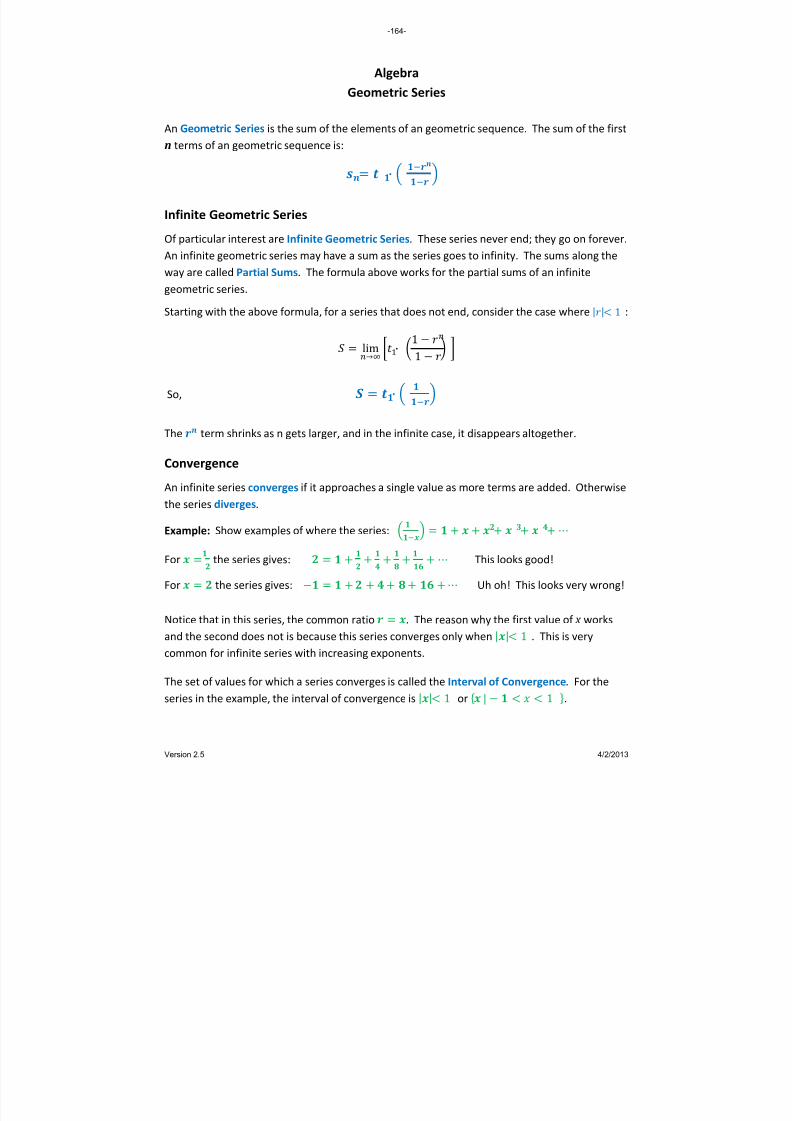
8/13/2019 AlgebraHandbook_very Helpful_ Print It
http://slidepdf.com/reader/full/algebrahandbookvery-helpful-print-it 164/178
Algebra
Geometric Series
An Geometric Series is the sum of the elements of an geometric sequence. The sum of the first
n terms of an geometric sequence is:
·
Infinite Geometric Series
Of particular interest are Infinite Geometric Series. These series never end; they go on forever.
An infinite geometric series may have a sum as the series goes to infinity. The sums along the
way are called Partial Sums. The formula above works for the partial sums of an infinite
geometric series.
Starting with the above formula, for a series that does not end, consider the case where || 1 :
lim · 1 1
So, ·
The term shrinks as n gets larger, and in the infinite case, it disappears altogether.
Convergence
An infinite series converges if it approaches a single value as more terms are added. Otherwise
the series diverges.
Example: Show examples of where the series:
For the series gives:
This looks good!
For the series gives: Uh oh! This looks very wrong!
Notice that in this series, the common ratio . The reason why the first value of x works
and the second does not is because this series converges only when || 1 . This is very
common for infinite series with increasing exponents.
The set of values for which a series converges is called the Interval of Convergence. For the
series in the example, the interval of convergence is || 1 or | 1 .
-164-
Version 2.5 4/2/2013

8/13/2019 AlgebraHandbook_very Helpful_ Print It
http://slidepdf.com/reader/full/algebrahandbookvery-helpful-print-it 165/178
Algebra
A Few Special Series
Series Involving
1 6
11 12 13 14
6
1 90
11 12 13 14 90
Series Involving e
1!
1 1 12! 13! 14! 15!
122! 1
1 12! 34! 56! 78! 910! 1
Cubes of Natural Numbers
Consider the
Series
of
cubes
of
the
natural
numbers:
n 1 2 3 4 5 6 7
1 8 27 54 125 216 343
1 9 36 100 225 441 784
So, the sums of cubes are squares. In fact successive sums are the squares of the Triangle
Numbers. The Triangle Numbers are the sums of the sequence of natural numbers:
n 1 2 3 4 5 6 7
1 2 3 4 5 6 7
1 3 6 10 15 21 28
-165-
Version 2.5 4/2/2013
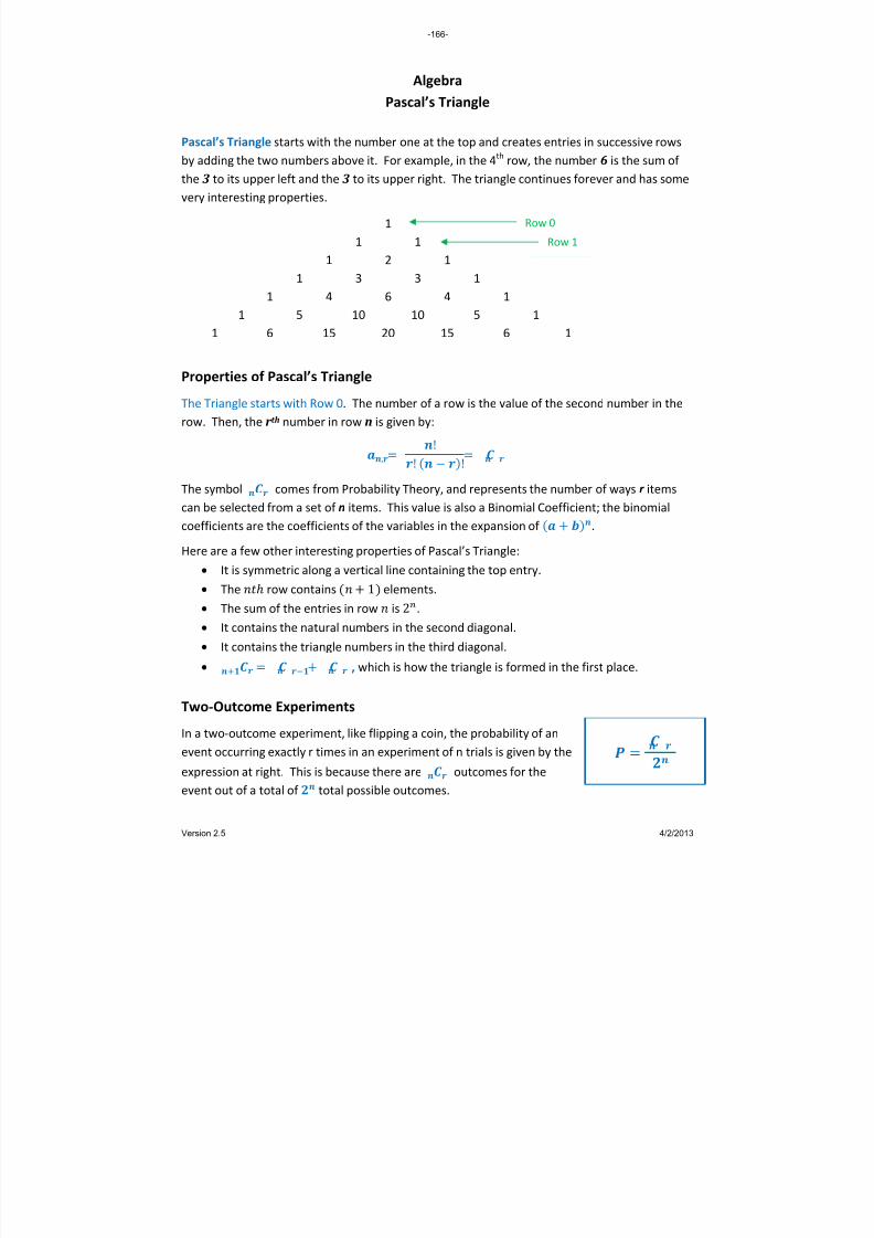
8/13/2019 AlgebraHandbook_very Helpful_ Print It
http://slidepdf.com/reader/full/algebrahandbookvery-helpful-print-it 166/178
Algebra
Pascal’s Triangle
Pascal’s Triangle starts with the number one at the top and creates entries in successive rows
by adding the two numbers above it. For example, in the 4th
row, the number 6 is the sum of
the 3 to its upper left and the 3 to its upper right. The triangle continues forever and has some
very interesting properties.
1
1 1
1 2 1
1 3 3 1
1 4 6 4 1
1 5 10 10 5 1
1
6
15
20
15
6
1
Properties of Pascal’s Triangle
The Triangle starts with Row 0. The number of a row is the value of the second number in the
row. Then, the r th number in row n is given by:
, !! !
The symbol
comes from Probability Theory, and represents the number of ways r items
can be
selected
from
a set
of
n items.
This
value
is
also
a Binomial
Coefficient;
the
binomial
coefficients are the coefficients of the variables in the expansion of .
Here are a few other interesting properties of Pascal’s Triangle:
• It is symmetric along a vertical line containing the top entry.
• The row contains 1 elements.
• The sum of the entries in row is 2.
• It contains the natural numbers in the second diagonal.
• It contains the triangle numbers in the third diagonal.
• , which
is
how
the
triangle
is
formed
in
the
first
place.
Two‐Outcome Experiments
In a two‐outcome experiment, like flipping a coin, the probability of an
event occurring exactly r times in an experiment of n trials is given by the
expression at right. This is because there are outcomes for the
event out of a total of total possible outcomes.
Row 0
Row 1
-166-
Version 2.5 4/2/2013

8/13/2019 AlgebraHandbook_very Helpful_ Print It
http://slidepdf.com/reader/full/algebrahandbookvery-helpful-print-it 167/178
Algebra
Binomial Expansion
4 Steps to a Constructing a Binomial Expansion
1. Start with the binomial coefficients
2. Add in the powers of the first term of the binomial
3. Add in the powers of the second term of the binomial
4. Simplify
Consider the following example: Expand and simplify
Step 1: Start with the binomial coefficients
40
41
42
43
44
Step 2: Add in the powers of the first term of the binomial
40 2 41 2 42 2 43 2 44 2 Step 3: Add in the powers of the second term of the binomial
40 2
3
41 2
3
42 2
3
43 2
3
44 2
3
Step 4: Simplify:
1161 483 649 4227 1181
Notice the following about the expansion:
1. There are
terms, where
is
the
exponent
of
the
binomial
being
expanded.
2. is the top number in every binomial coefficient.
3. The bottom numbers in the binomial coefficients count up from 0 to .
4. When a term of the original binomial is negative, the signs in the solution alternate.
5. The exponent of the first term in the original binomial counts down from to 0.
6. The exponent of the second term in the original binomial counts up from 0 to .
7. The exponents of the two terms in the original binomial add to in every term of the
expansion.
-167-
Version 2.5 4/2/2013
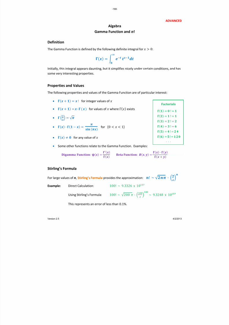
8/13/2019 AlgebraHandbook_very Helpful_ Print It
http://slidepdf.com/reader/full/algebrahandbookvery-helpful-print-it 168/178
ADVANCED Algebra
Gamma Function and n!
Definition
The Gamma Function is defined by the following definite integral for 0:
Initially, this integral appears daunting, but it simplifies nicely under certain conditions, and has some very interesting properties.
Properties and Values The following properties and values of the Gamma Function are of particular interest:
• ! for integer values of • · for values of where Γ exists •
√ • ·
for 0 1
• for any value of • Some other functions relate to the Gamma Function. Examples:
: : , ·
Stirling’s Formula For large values of n, Stirling’s Formula provides the approximation: ! ~ √ · Example: Direct Calculation: 100! ~ 9.3326 x 10
Using Stirling’s Formula: 100! ~ √ 200 · ~ 9.3248 x 10
This represents an error of less than 0.1%.
! ! ! ! ! !
. . .
Factorials
-168-
Version 2.5 4/2/2013

8/13/2019 AlgebraHandbook_very Helpful_ Print It
http://slidepdf.com/reader/full/algebrahandbookvery-helpful-print-it 169/178

8/13/2019 AlgebraHandbook_very Helpful_ Print It
http://slidepdf.com/reader/full/algebrahandbookvery-helpful-print-it 170/178
Page Subject
15 Absolute Value
Absolute Value Functions
47 Equations
48 Inequalities
16 Algebraic Properties
161 Arithmetic Mean
16 Associative Property
Asymptotes
148, 149 Conic Sections
109 Exponential Functions
169 Gamma Function
111 ‐113 Logarithmic Functions
130 ‐136 Rational Functions
167 Binomial Expansion
Box Method
62 Multiplying Binomials
63 Multiplying Polynomials
10 Cartesian Plane
144 Circles
16 Closure Property
22 Combinations16 Commutative Property
Complex Numbers
80 Absolute Value
81 Adding and Subtracting
80 Conjugate
80 Definition
83 Graphical Representation
81 Multiplying and Dividing
84 Operations in Polar Coordinates
107 Condensing a Logarithmic ExpressionConic Equations
141, 149 Characteristics
152 Classification
153 Manipulation
Algebra Handbook Index
-170-
Version 2.5 4/2/2013

8/13/2019 AlgebraHandbook_very Helpful_ Print It
http://slidepdf.com/reader/full/algebrahandbookvery-helpful-print-it 171/178
Page Subject
Algebra Handbook Index
Conic Sections
140 Definitions
154 Parametric Equations
(also see entries for specific curves)
52, 53 Consistent Lines
105 Converting Between Exponential and Logarithmic Expressions
10 Coordinates in a Plane
Cramer's Rule
96 2 Equations
97 3 Equations
120 Cubic Equations ‐Sum and Difference Formulas
116 Decay (Exponential)
52, 53 Dependent Lines
124 Descartes’ Rule of Signs
Determinants
93 2x2 Matrix
95 General Case
16 Distributive Property
64 Dividing Polynomials
103 e
Ellipse146 Centered at Point (h, k)
145 Centered on the Origin (Standard Position)
147 Polar Form
72 Equations ‐Solving by Factoring
103 Euler's Equation
106 Expanding a Logarithmic Expression
117 Exponential Equations
Exponential Function Graphs
109 Graphing a Function
110, 115 Sample GraphsExponents
105 Converting an Exponential Expression to Logarithmic Form
117 Exponential Equations
116 Exponential Functions ‐Growth, Decay, Interest
56 Formulas
104 Table of Exponents
-171-
Version 2.5 4/2/2013

8/13/2019 AlgebraHandbook_very Helpful_ Print It
http://slidepdf.com/reader/full/algebrahandbookvery-helpful-print-it 172/178
Page Subject
Algebra Handbook Index
168 Factorials
Factoring
69 AC Method
70 Brute Force Method
71 Quadratic Formula Method
68 Simple Case Method
156 Fibonacci Sequence
62 FOIL Method of Multiplying Binomials
Functions
26 Adding and Subtracting
27 Compositions
24 Definitions
116 Exponential (Growth, Decay, Interest)
115 Graphs of Various Functions
28 Inverses
24 Line Tests
26 Multiplying and Dividing
26 Notation
26 Operations
29 Transformation ‐Building a Graph
Gamma Function169 Gamma Function ‐Calculating
168 Gamma Function ‐Definition
169 Gamma Function ‐Graphing
94 Gauss‐Jordan Elimination
161 Geometric Mean
156 Golden Ratio (f )
Graph (look up the type of curve you are trying to graph)25 Greatest Integer Function
116 Growth (Exponential)
162 Harmonic MeanHyperbola
149 Centered at Point (h, k)
148 Centered on the Origin (Standard Position)
150 Polar Form
151 Polar Form ‐Construction Over the Domain: 0 to 2π
80 i
-172-
Version 2.5 4/2/2013

8/13/2019 AlgebraHandbook_very Helpful_ Print It
http://slidepdf.com/reader/full/algebrahandbookvery-helpful-print-it 173/178
Page Subject
Algebra Handbook Index
16 Identity Property
Imaginary Numbers
80 i
80 Definition
83 Powers of i
82 Square Root of i
52, 53 Inconsistent Lines
52, 53 Independent Lines
Inequalities
44 Compound in One Dimension
43 Graphs in One Dimension
46 Graphs in Two Dimensions
45 Two Dimensions
14 Integers
Integer Functions
25 Greatest Integer Function
25 Least Integer Functions
25 Nearest Integer Functions
Intersection of Curves
128 Circle and Ellipse
126 General Case127 Line and Parabola
126 Lines
16 Inverse Property
25 Least Integer Functions
53 Linear Dependence
Linear Equations
38 Point‐Slope Form of a Line
38 Slope‐Intercept Form of a Line
38 Standard Form of a Line
11 Linear Patterns112 ln
117 Logarithmic Equations
Logarithmic Function Graphs
111 Graphing Methods
114, 115 Sample Graphs
-173-
Version 2.5 4/2/2013

8/13/2019 AlgebraHandbook_very Helpful_ Print It
http://slidepdf.com/reader/full/algebrahandbookvery-helpful-print-it 174/178
Page Subject
Algebra Handbook Index
Logarithms
107, 108 Condensing a Logarithmic Expression
105 Converting a Logarithmic Expression to Exponential Form
106 Expanding a Logarithmic Expression
102 Formulas
117 Logarithmic Equations
104 Table of Logarithms
64 Long Division of Polynomials
Matrices
90 Addition
98 Augmented Matrices
99 Augmented Matrix Examples (2x2)
100 Augmented Matrix Example (3x3)
92 Division
92 Identity Matrices
93 Inverse of a 2x2 Matrix
94 Inverse of a General Matrix
91 Multiplication
90 Scalar Multiplication
161, 162 Means ‐Pythagorean
63 Multiplying PolynomialsMulti‐Step Equations
18 Reverse PEMDAS
19 Tips and Tricks
168 n !
112 Natural Logarithms
14 Natural Numbers
25 Nearest Integer Functions
Number Patterns
13 Completing Number Patterns
11 Converting a Linear Pattern to an Equation12 Identifying Number Patterns
11 Recognizing Linear Patterns
14 Number Sets ‐Basic
20 Odds
15 Operating with Real Numbers
-174-
Version 2.5 4/2/2013

8/13/2019 AlgebraHandbook_very Helpful_ Print It
http://slidepdf.com/reader/full/algebrahandbookvery-helpful-print-it 175/178
Page Subject
Algebra Handbook Index
Order of Operations
9 Parenthetical Device
9 PEMDAS
Parabola
142 Vertex at Point (h, k)
141 Vertex at the Origin (Standard Position)
143 Polar Form
Parallel and Perpendicular Lines
39 Parallel and Perpendicular Lines ‐Slopes
41 Parallel, Coincident or Intersecting Lines ‐Flowchart
40 Parallel, Perpendicular or Neither Lines ‐Flowchart
Parametric Equations
154 Conic Sections
55 General
9 Parenthetical Device
166 Pascal’s Triangle
9 PEMDAS
10 Plotting Points on a Coordinate Plane
38 Point‐Slope Form of a Line
83, 84 Polar Coordinates
Polynomials61 Adding and Subtracting
60 Definition
60 Degree
124 Polynomials – Developing Possible Roots
65 Factoring
119 Finding Extrema with Derivatives
118 Graphs
65 Greatest Common Factor
62 Multiplying Binomials (FOIL, Box, Numerical Methods)
61 Standard Form120 Sum and Difference of Cubes
122, 123 Synthetic Division
125 Testing Possible Roots
121 Variable Substitution
75 Powers and Roots Table
-175-
Version 2.5 4/2/2013

8/13/2019 AlgebraHandbook_very Helpful_ Print It
http://slidepdf.com/reader/full/algebrahandbookvery-helpful-print-it 176/178
Page Subject
Algebra Handbook Index
Probability
20 Probability and Odds
21 Probability with Dice
Properties of Algebra
16 Properties of Addition and Multiplication
16 Properties of Equality
16 Properties of Zero
Properties of Inequality
42 Addition and Subtraction
42 Multiplication and Division
161, 162 Pythagorean Means
85 Quadratic Equations ‐Complex Solutions
76 Quadratic Formula
Quadratic Functions
74 Completing the Square
67 Differences of Squares
79 Fitting with Three Points
73 Opening Up or Down
66 Perfect Squares
73 Standard Form
73 Vertex and Axis of Symmetry73 Vertex Form
77 Quadratic Inequalities in One Variable
88, 89 Radical Equations
138 Rational Equations
Rational Expressions
137 Addition and Subtraction
137 Multiplication and Division
Rational Functions
129 Domain
133 General Rational Functions130 Holes and Asymptotes
132 Simple Rational Functions
139 Rational Inequalities
14 Rational Numbers
17 Reflexive Property
14 Real Numbers
-176-
Version 2.5 4/2/2013

8/13/2019 AlgebraHandbook_very Helpful_ Print It
http://slidepdf.com/reader/full/algebrahandbookvery-helpful-print-it 177/178
Page Subject
Algebra Handbook Index
Roots
124, 125 Polynomials (i.e., zeros)
86 Radical Rules
86 Rationalizing the Denominator
87 Simplifying Square Roots
Scientific Notation
58 Adding and Subtracting
57 Conversion to and from Decimals
57 Format
59 Multiplying and Dividing
Sequences
159 Arithmetic
155 Definitions
156 Fibonacci Sequence
163 Geometric
Series
160 Arithmetic
155 Definitions
164 Geometric
165 Special (π, e, cubes)
158 Summation Formulas157 Summation Notation and Properties
Signs
15 Signs of Added or Subtracted Numbers
15 Signs of Multiplied or Divided Numbers
Slope
37 Slope of a Line ‐8 Variations
35 Slope of a Line ‐Mathematical Definition
36 Slope of a Line ‐Rise over Run
38 Slope‐Intercept Form of a Line
39 Slopes of Parallel and Perpendicular Lines62 Stacked Polynomial Method of Multiplying Binomials
63 Stacked Polynomial Method of Multiplying Polynomials
38 Standard Form of a Line
23 Statistical Measures
168 Stirling's Formula
17 Substitution Property
-177-
Version 2.5 4/2/2013

8/13/2019 AlgebraHandbook_very Helpful_ Print It
http://slidepdf.com/reader/full/algebrahandbookvery-helpful-print-it 178/178
Page Subject
Algebra Handbook Index
Summation (S)
158 Formulas
157 Notation and Properties
17 Symmetric Property
Synthetic Division
123 Synthetic Division ‐Comparison to Long Division
122 Synthetic Division ‐Process
Systems of Equations
52 Classification
51 Elimination Method
49 Graphing a Solution
50 Substitution Method
54 Systems of Inequalities ‐Two Dimensions
Transformations
-178-


