Algebraic Geometry

J.S. Milne

Taiaroa PublishingErehwon

Version 5.00February 20, 2005

Abstract

These notes are an introduction to the theory of algebraic varieties. In contrast to mostsuch accounts they study abstract algebraic varieties, and not just subvarieties of affine andprojective space. This approach leads more naturally into scheme theory.

v2.01 (August 24, 1996). First version on the web.v3.01 (June 13, 1998).v4.00 (October 30, 2003). Fixed errors; many minor revisions; added exercises; added two

sections; 206 pages.v5.00 (February 20, 2005). Heavily revised; most numbering changed; 227 pages.

Please send comments and lists of corrections to me at math@jmilne.org

Available at http://www.jmilne.org/math/

Copyright c© 1996, 1998, 2003, 2005. J.S. Milne.

This work is licensed under aCreative Commons Licence (Attribution-NonCommercial-NoDerivs 2.0)http://creativecommons.org/licenses/by-nc-nd/2.0/

Contents

Introduction 3

1 Preliminaries 4Algebras 4; Ideals 4; Noetherian rings 6; Unique factorization 8; Polynomial rings 10;Integrality 11; Direct limits (summary) 13; Rings of fractions 14; Tensor Products 17;Categories and functors 20; Algorithms for polynomials 22; Exercises 28

2 Algebraic Sets 29Definition of an algebraic set 29; The Hilbert basis theorem 30; The Zariski topology 31;The Hilbert Nullstellensatz 31; The correspondence between algebraic sets and ideals 32;Finding the radical of an ideal 35; The Zariski topology on an algebraic set 36; The coor-dinate ring of an algebraic set 36; Irreducible algebraic sets 37; Dimension 40; Exercises42

3 Affine Algebraic Varieties 43Ringed spaces 43; The ringed space structure on an algebraic set 44; Morphisms of ringedspaces 47; Affine algebraic varieties 48; The category of affine algebraic varieties 49;Explicit description of morphisms of affine varieties 50; Subvarieties 53; Properties of theregular map defined by specm(α) 54; Affine space without coordinates 54; Exercises 56

4 Algebraic Varieties 57Algebraic prevarieties 57; Regular maps 58; Algebraic varieties 59; Maps from varieties toaffine varieties 60; Subvarieties 60; Prevarieties obtained by patching 61; Products of vari-eties 62; The separation axiom revisited 67; Fibred products 69; Dimension 70; Birationalequivalence 71; Dominating maps 72; Algebraic varieties as a functors 72; Exercises 74

5 Local Study 75Tangent spaces to plane curves 75; Tangent cones to plane curves 76; The local ring at apoint on a curve 77; Tangent spaces of subvarieties of Am 78; The differential of a regularmap 79; Etale maps 81; Intrinsic definition of the tangent space 83; Nonsingular points 85;Nonsingularity and regularity 87; Nonsingularity and normality 88; Etale neighbourhoods88; Smooth maps 90; Dual numbers and derivations 91; Tangent cones 94; Exercises 95

6 Projective Varieties 97Algebraic subsets of Pn 97; The Zariski topology on Pn 100; Closed subsets of An andPn 100; The hyperplane at infinity 101; Pn is an algebraic variety 102; The homogeneouscoordinate ring of a subvariety of Pn 103; Regular functions on a projective variety 104;Morphisms from projective varieties 105; Examples of regular maps of projective vari-eties 107; Projective space without coordinates 111; Grassmann varieties 111; Bezout’stheorem 115; Hilbert polynomials (sketch) 116; Exercises 117

7 Complete varieties 118Definition and basic properties 118; Projective varieties are complete 119; Eliminationtheory 121; The rigidity theorem 123; Theorems of Chow 124; Nagata’s Embedding Prob-lem 124; Exercises 125

8 Finite Maps 126

Definition and basic properties 126; Noether Normalization Theorem 130; Zariski’s maintheorem 131; The base change of a finite map 133; Proper maps 133; Exercises 134

9 Dimension Theory 135Affine varieties 135; Projective varieties 141

10 Regular Maps and Their Fibres 144Constructible sets 144; Orbits of group actions 147; The fibres of morphisms 148; Thefibres of finite maps 150; Flat maps 152; Lines on surfaces 153; Stein factorization 158;Exercises 158

11 Algebraic spaces; geometry over an arbitrary field 160Preliminaries 160; Affine algebraic spaces 163; Affine algebraic varieties. 164; Algebraicspaces; algebraic varieties. 165; Local study 169; Projective varieties. 171; Completevarieties. 171; Normal varieties; Finite maps. 171; Dimension theory 171; Regular mapsand their fibres 172; Algebraic groups 172; Exercises 173

12 Divisors and Intersection Theory 174Divisors 174; Intersection theory. 175; Exercises 179

13 Coherent Sheaves; Invertible Sheaves 180Coherent sheaves 180; Invertible sheaves. 182; Invertible sheaves and divisors. 183; Directimages and inverse images of coherent sheaves. 184; Principal bundles 185

14 Differentials (Outline) 186

15 Algebraic Varieties over the Complex Numbers (Outline) 188

16 Descent Theory 191Models 191; Fixed fields 191; Descending subspaces of vector spaces 192; Descendingsubvarieties and morphisms 193; Galois descent of vector spaces 194; Descent data 196;Galois descent of varieties 198; Weil restriction 199; Generic fibres 200; Rigid descent200; Weil’s descent theorems 202; Restatement in terms of group actions 204; Faithfullyflat descent 206

17 Lefschetz Pencils (Outline) 209Definition 209

18 Algebraic Schemes 211

A Solutions to the exercises 212

B Annotated Bibliography 219

Index 221

1

Introduction

Just as the starting point of linear algebra is the study of the solutions of systems of linearequations,

n∑j=1

aijXj = bi, i = 1, . . . ,m, (1)

the starting point for algebraic geometry is the study of the solutions of systems of polyno-mial equations,

fi(X1, . . . , Xn) = 0, i = 1, . . . ,m, fi ∈ k[X1, . . . , Xn].

Note immediately one difference between linear equations and polynomial equations: the-orems for linear equations don’t depend on which field k you are working over,1 but thosefor polynomial equations depend on whether or not k is algebraically closed and (to a lesserextent) whether k has characteristic zero.

A better description of algebraic geometry is that it is the study of polynomial functionsand the spaces on which they are defined (algebraic varieties), just as topology is the studyof continuous functions and the spaces on which they are defined (topological spaces),differential topology the study of infinitely differentiable functions and the spaces on whichthey are defined (differentiable manifolds), and so on:

algebraic geometry regular (polynomial) functions algebraic varieties

topology continuous functions topological spaces

differential topology differentiable functions differentiable manifolds

complex analysis analytic (power series) functions complex manifolds.

The approach adopted in this course makes plain the similarities between these differentareas of mathematics. Of course, the polynomial functions form a much less rich class thanthe others, but by restricting our study to polynomials we are able to do calculus over anyfield: we simply define

d

dX

∑aiX

i =∑

iaiXi−1.

Moreover, calculations (on a computer) with polynomials are easier than with more generalfunctions.

Consider a nonzero differentiable function f(x, y, z). In calculus, we learn that theequation

f(x, y, z) = C (2)

defines a surface S in R3, and that the tangent plane to S at a point P = (a, b, c) hasequation2 (

∂f

∂x

)P

(x− a) +(∂f

∂y

)P

(y − b) +(∂f

∂z

)P

(z − c) = 0. (3)

1For example, suppose that the system (1) has coefficients aij ∈ k and that K is a field containing k. Then(1) has a solution in kn if and only if it has a solution in Kn, and the dimension of the space of solutions is thesame for both fields. (Exercise!)

2Think of S as a level surface for the function f , and note that the equation is that of a plane through (a, b, c)perpendicular to the gradient vector (Of)P of f at P .

2

The inverse function theorem says that a differentiable map α : S → S′ of surfaces is alocal isomorphism at a point P ∈ S if it maps the tangent plane at P isomorphically ontothe tangent plane at P ′ = α(P ).

Consider a nonzero polynomial f(x, y, z) with coefficients in a field k. In this course,we shall learn that the equation (2) defines a surface in k3, and we shall use the equation(3) to define the tangent space at a point P on the surface. However, and this is one of theessential differences between algebraic geometry and the other fields, the inverse functiontheorem doesn’t hold in algebraic geometry. One other essential difference is that 1/X isnot the derivative of any rational function of X , and nor is Xnp−1 in characteristic p 6= 0— these functions can not be integrated in the ring of polynomial functions.

The first ten sections of the notes form a basic course on algebraic geometry. In thesesections we generally assume that the ground field is algebraically closed in order to be ableto concentrate on the geometry. The remaining sections treat more advanced topics, and arelargely independent of one another except that Section 11 should be read first.

The approach to algebraic geometry taken in these notes

In differential geometry it is important to define differentiable manifolds abstractly, i.e., notas submanifolds of some Euclidean space. For example, it is difficult even to make senseof a statement such as “the Gauss curvature of a surface is intrinsic to the surface but theprincipal curvatures are not” without the abstract notion of a surface.

Until the mid 1940s, algebraic geometry was concerned only with algebraic subvarietiesof affine or projective space over algebraically closed fields. Then, in order to give substanceto his proof of the congruence Riemann hypothesis for curves an abelian varieties, Weilwas forced to develop a theory of algebraic geometry for “abstract” algebraic varieties overarbitrary fields,3 but his “foundations” are unsatisfactory in two major respects:

— Lacking a topology, his method of patching together affine varieties to form abstractvarieties is clumsy.

— His definition of a variety over a base field k is not intrinsic; specifically, he fixessome large “universal” algebraically closed field Ω and defines an algebraic varietyover k to be an algebraic variety over Ω with a k-structure.

In the ensuing years, several attempts were made to resolve these difficulties. In 1955,Serre resolved the first by borrowing ideas from complex analysis and defining an algebraicvariety over an algebraically closed field to be a topological space with a sheaf of functionsthat is locally affine.4 Then, in the late 1950s Grothendieck resolved all such difficulties byintroducing his theory of schemes.

In these notes, we follow Grothendieck except that, by working only over a base field,we are able to simplify his language by considering only the closed points in the underlyingtopological spaces. In this way, we hope to provide a bridge between the intuition given bydifferential geometry and the abstractions of scheme theory.

Notations

We use the standard (Bourbaki) notations: N = 0, 1, 2, . . ., Z = ring of integers, R =field of real numbers, C = field of complex numbers, Fp = Z/pZ = field of p elements, p a

3Weil, Andre. Foundations of algebraic geometry. American Mathematical Society, Providence, R.I. 1946.4Serre, Jean-Pierre. Faisceaux algebriques coherents. Ann. of Math. (2) 61, (1955). 197–278.

3

prime number. Given an equivalence relation, [∗] denotes the equivalence class containing∗. A family of elements of a set A indexed by a second set I , denoted (ai)i∈I , is a functioni 7→ ai : I → A.

A field k is said to be separably closed if it has no finite separable extensions of degree> 1. We use ksep and kal to denote separable and algebraic closures of k respectively.

All rings will be commutative with 1, and homomorphisms of rings are required to map1 to 1. A k-algebra is a ring A together with a homomorphism k → A. For a ring A, A× isthe group of units in A:

A× = a ∈ A | there exists a b ∈ A such that ab = 1.

We use Gothic (fraktur) letters for ideals:

a b c m n p q A B C M N P Q

a b c m n p q A B C M N P Q

Xdf= Y X is defined to be Y , or equals Y by definition;

X ⊂ Y X is a subset of Y (not necessarily proper, i.e., X may equal Y );X ≈ Y X and Y are isomorphic;X ' Y X and Y are canonically isomorphic (or there is a given or unique isomorphism).

References

Atiyah and MacDonald 1969: Introduction to Commutative Algebra, Addison-Wesley.Cox et al. 1992: Varieties, and Algorithms, Springer.FT: Milne, J.S., Fields and Galois Theory, v5.00, 2005 (www.jmilne.org/math/).Hartshorne 1977: Algebraic Geometry, Springer.Mumford 1999: The Red Book of Varieties and Schemes, Springer.Shafarevich 1994: Basic Algebraic Geometry, Springer.

For other references, see the annotated bibliography at the end.

Prerequisites

The reader is assumed to be familiar with the basic objects of algebra, namely, rings, mod-ules, fields, and so on, and with transcendental extensions of fields (FT, Section 8).

Acknowledgements

I thank the following for providing corrections and comments on earlier versions of thesenotes: Sandeep Chellapilla, Shalom Feigelstock, B.J. Franklin, Guido Helmers, Jasper LoyJiabao, David Rufino, Tom Savage, and others.

4 1 PRELIMINARIES

1 Preliminaries

In this section, we review some definitions and basic results in commutative algebra andcategory theory, and we derive some algorithms for working in polynomial rings.

Algebras

Let A be a ring. An A-algebra is a ring B together with a homomorphism iB : A → B. Ahomomorphism of A-algebras B → C is a homomorphism of rings ϕ : B → C such thatϕ(iB(a)) = iC(a) for all a ∈ A.

Elements x1, . . . , xn of anA-algebraB are said to generate it if every element ofB canbe expressed as a polynomial in the xi with coefficients in iB(A), i.e., if the homomorphismof A-algebras A[X1, . . . , Xn] → B sending Xi to xi is surjective. We then write B =(iBA)[x1, . . . , xn]. An A-algebra B is said to be finitely generated (or of finite-type overA) if it is generated by a finite set of elements.

A ring homomorphism A → B is finite, and B is a finite5 A-algebra, if B is finitelygenerated as an A-module.

Let k be a field, and letA be a k-algebra. When 1 6= 0 inA, the map k → A is injective,and we can identify k with its image, i.e., we can regard k as a subring of A. When 1 = 0in a ring A, then A is the zero ring, i.e., A = 0.

Let A[X] be the polynomial ring in the symbol X with coefficients in A. If A is anintegral domain, then deg(fg) = deg(f) + deg(g), and it follows that A[X] is also anintegral domain; moreover, A[X]× = A×.

Ideals

Let A be a ring. A subring of A is a subset containing 1 that is closed under addition,multiplication, and the formation of negatives. An ideal a in A is a subset such that

(a) a is a subgroup of A regarded as a group under addition;(b) a ∈ a, r ∈ A⇒ ra ∈ a.

The ideal generated by a subset S of A is the intersection of all ideals a containing A— it is easy to verify that this is in fact an ideal, and that it consists of all finite sums of theform

∑risi with ri ∈ A, si ∈ S. When S = s1, s2, . . ., we shall write (s1, s2, . . .) for

the ideal it generates.Let a and b be ideals in A. The set a+ b | a ∈ a, b ∈ b is an ideal, denoted by a + b.

The ideal generated by ab | a ∈ a, b ∈ b is denoted by ab. Clearly ab consists of allfinite sums

∑aibi with ai ∈ a and bi ∈ b, and if a = (a1, . . . , am) and b = (b1, . . . , bn),

then ab = (a1b1, . . . , aibj , . . . , ambn). Note that ab ⊂ a ∩ b.Let a be an ideal of A. The set of cosets of a in A forms a ring A/a, and a 7→ a + a

is a homomorphism ϕ : A → A/a. The map b 7→ ϕ−1(b) is a one-to-one correspondencebetween the ideals of A/a and the ideals of A containing a.

An ideal p is prime if p 6= A and ab ∈ p⇒ a ∈ p or b ∈ p. Thus p is prime if and onlyif A/p is nonzero and has the property that

ab = 0, b 6= 0⇒ a = 0,

i.e., A/p is an integral domain.

5The term “module-finite” is also used.

Ideals 5

An ideal m is maximal if m 6= A and there does not exist an ideal n contained strictlybetween m and A. Thus m is maximal if and only if A/m is nonzero and has no propernonzero ideals, and so is a field. Note that

m maximal =⇒ m prime.

The ideals of A × B are all of the form a × b with a and b ideals in A and B. To seethis, note that if c is an ideal in A × B and (a, b) ∈ c, then (a, 0) = (1, 0)(a, b) ∈ c and(0, b) = (0, 1)(a, b) ∈ c. Therefore, c = a× b with

a = a | (a, 0) ∈ c, b = b | (0, b) ∈ c.

THEOREM 1.1 (CHINESE REMAINDER THEOREM). Let a1, . . . , an be ideals in a ring A.If ai is coprime to aj (i.e., ai + aj = A) whenever i 6= j, then the map

A→ A/a1 × · · · ×A/an (4)

is surjective, with kernel∏

ai =⋂

ai.

PROOF. Suppose first that n = 2. As a1+a2 = A, there exist ai ∈ ai such that a1+a2 = 1.Then x = a1x2+a2x1 maps to (x1 mod a1, x2 mod a2), which shows that (4) is surjective.

For each i, there exist elements ai ∈ a1 and bi ∈ ai such that

ai + bi = 1, all i ≥ 2.

The product∏i≥2(ai + bi) = 1, and lies in a1 +

∏i≥2 ai, and so

a1 +∏i≥2

ai = A.

We can now apply the theorem in the case n = 2 to obtain an element y1 of A such that

y1 ≡ 1 mod a1, y1 ≡ 0 mod∏i≥2

ai.

These conditions imply

y1 ≡ 1 mod a1, y1 ≡ 0 mod aj , all j > 1.

Similarly, there exist elements y2, ..., yn such that

yi ≡ 1 mod ai, yi ≡ 0 mod aj for j 6= i.

The element x =∑xiyi maps to (x1 mod a1, . . . , xn mod an), which shows that (4) is

surjective.It remains to prove that

⋂ai =

∏ai. We have already noted that

⋂ai ⊃

∏ai. First

suppose that n = 2, and let a1 + a2 = 1, as before. For c ∈ a1 ∩ a2, we have

c = a1c+ a2c ∈ a1 · a2

which proves that a1 ∩ a2 = a1a2. We complete the proof by induction. This allows usto assume that

∏i≥2 ai =

⋂i≥2 ai. We showed above that a1 and

∏i≥2 ai are relatively

prime, and soa1 · (

∏i≥2

ai) = a1 ∩ (∏i≥2

ai) =⋂

ai.

2

6 1 PRELIMINARIES

Noetherian rings

PROPOSITION 1.2. The following conditions on a ring A are equivalent:(a) every ideal in A is finitely generated;(b) every ascending chain of ideals a1 ⊂ a2 ⊂ · · · eventually becomes constant, i.e., for

some m, am = am+1 = · · · .(c) every nonempty set of ideals in A has a maximal element (i.e., an element not prop-

erly contained in any other ideal in the set).

PROOF. (a) =⇒ (b): If a1 ⊂ a2 ⊂ · · · is an ascending chain, then a =⋃

ai is an ideal,and hence has a finite set a1, . . . , an of generators. For some m, all the ai belong am andthen

am = am+1 = · · · = a.

(b) =⇒ (c): Let S be a nonempty set of ideals inA. Let a1 ∈ S; if a1 is not maximal inS, then there exists an ideal a2 in S properly containing a1. Similarly, if a2 is not maximalin S, then there exists an ideal a3 in S properly containing a2, etc.. In this way, we obtainan ascending chain of ideals a1 ⊂ a2 ⊂ a3 ⊂ · · · in S that will eventually terminate in anideal that is maximal in S.

(c) =⇒ (a): Let a be an ideal, and let S be the set of ideals b ⊂ a that are finitelygenerated. Then S is nonempty and so it contains a maximal element c = (a1, . . . , ar). Ifc 6= a, then there exists an element a ∈ arc, and (a1, . . . , ar, a) will be a finitely generatedideal in a properly containing c. This contradicts the definition of c. 2

A ring A is noetherian if it satisfies the conditions of the proposition. Note that, in anoetherian ring, every proper ideal is contained in a maximal ideal (apply (c) to the set ofall proper ideals of A containing the given ideal). In fact, this is true in any ring, but theproof for non-noetherian rings uses the axiom of choice (FT 6.4).

A ringA is said to be local if it has exactly one maximal ideal m. Because every nonunitis contained in a maximal ideal, for a local ring A× = Ar m.

PROPOSITION 1.3 (NAKAYAMA’S LEMMA). Let A be a local noetherian ring with maxi-mal ideal m, and let M be a finitely generated A-module.

(a) If M = mM , then M = 0.(b) If N is a submodule of M such that M = N + mM , then M = N .

PROOF. (a) Let x1, . . . , xn generate M , and write

xi =∑j

aijxj

for some aij ∈ m. Then x1, . . . , xn are solutions to the system of n equations in n variables∑j

(δij − aij)xj = 0, δij = Kronecker delta,

and so Cramer’s rule tells us that det(δij−aij) ·xi = 0 for all i. But det(δij−aij) expandsout as 1 plus a sum of terms in m. In particular, det(δij − aij) /∈ m, and so it is a unit. Itfollows that all the xi are zero, and so M = 0.

(b) The hypothesis implies that M/N = m(M/N), and so M/N = 0, i.e., M = N . 2

Noetherian rings 7

Now let A be a local noetherian ring with maximal ideal m. When we regard m as anA-module, the action of A on m/m2 factors through k = A/m.

COROLLARY 1.4. The elements a1, . . . , an of m generate m as an ideal if and only if theirresidues modulo m2 generate m/m2 as a vector space over k. In particular, the minimumnumber of generators for the maximal ideal is equal to the dimension of the vector spacem/m2.

PROOF. If a1, . . . , an generate m, it is obvious that their residues generate m/m2. Con-versely, suppose that their residues generate m/m2, so that m = (a1, . . . , an)+m2. SinceAis noetherian and (hence) m is finitely generated, Nakayama’s lemma, applied with M = m

and N = (a1, . . . , an), shows that m = (a1, . . . , an). 2

DEFINITION 1.5. Let A be a noetherian ring.(a) The height ht(p) of a prime ideal p in A is the greatest length of a chain of prime

idealsp = pd ' pd−1 ' · · · ' p0. (5)

(b) The Krull dimension of A is supht(p) | p ⊂ A, p prime.

Thus, the Krull dimension of a ring A is the supremum of the lengths of chains ofprime ideals in A (the length of a chain is the number of gaps, so the length of (5) is d).For example, a field has Krull dimension 0, and conversely an integral domain of Krulldimension 0 is a field. The height of every nonzero prime ideal in principal ideal domain is1, and so such a ring has Krull dimension 1 (provided it is not a field).

The height of any prime ideal in a noetherian ring is finite, but the Krull dimension ofthe ring may be infinite (for an example of this, see Nagata, Local Rings, 1962, AppendixA.1). In Nagata’s nasty example, there are maximal ideals p1, p2, p3, ... in A such that thesequence ht(pi) tends to infinity.

DEFINITION 1.6. A local noetherian ring of Krull dimension d is said to be regular if itsmaximal ideal can be generated by d elements.

It follows from Corollary 1.4 that a local noetherian ring is regular if and only if itsKrull dimension is equal to the dimension of the vector space m/m2.

LEMMA 1.7. Let A be a noetherian ring. Any set of generators for an ideal in A containsa finite generating subset.

PROOF. Let a be the ideal generated by a subset S of A. Then a = (a1, . . . , an) for someai ∈ A. Each ai lies in the ideal generated by a finite subset Si of S. Now

⋃Si is finite and

generates a. 2

THEOREM 1.8 (KRULL INTERSECTION THEOREM). In any noetherian local ring A withmaximal ideal m,

⋂n≥1 mn = 0.

PROOF. Let a1, . . . , ar generate m. Then mn is generated by the monomials of degree n inthe ai. In other words, mn consists of the elements of A that equal g(a1, . . . , ar) for somehomogeneous polynomial g(X1, . . . , Xr) ∈ A[X1, . . . , Xr] of degree n. Let Sm be the setof homogeneous polynomials f of degree m such that f(a1, . . . , ar) ∈

⋂n≥1 mn, and let

a be the ideal generated by all the Sm. According to the lemma, there exists a finite set

8 1 PRELIMINARIES

f1, . . . , fs of elements of⋃Sm that generate a. Let di = deg fi, and let d = max di. Let

b ∈⋂n≥1 mn; in particular, b ∈ md+1, and so b = f(a1, . . . , ar) for some homogeneous f

of degree d+ 1. By definition, f ∈ Sd+1 ⊂ a, and so

f = g1f1 + · · ·+ gsfs

for some gi ∈ A. As f and the fi are homogeneous, we can omit from each gi all terms notof degree deg f − deg fi, since these terms cancel out. Thus, we may choose the gi to behomogeneous of degree deg f − deg fi = d+ 1− di > 0. Then

b = f(a1, . . . , ar) =∑

gi(a1, . . . , ar)fi(a1, . . . , ar) ∈ m ·⋂

mn.

Thus,⋂

mn = m ·⋂

mn, and Nakayama’s lemma implies that⋂

mn = 0. 2

Unique factorization

Let A be an integral domain. An element a of A is irreducible if it is not zero, not a unit,and admits only trivial factorizations, i.e.,

a = bc =⇒ b or c is a unit.

If every nonzero nonunit in A can be written as a finite product of irreducible elementsin exactly one way (up to units and the order of the factors), then A is called a uniquefactorization domain. In such a ring, an irreducible element a can divide a product bc onlyif it is an irreducible factor of b or c (write bc = aq and express b, c, q as products ofirreducible elements).

PROPOSITION 1.9. Let (a) be a nonzero proper principal ideal in an integral domain A.If (a) is a prime ideal, then a is irreducible, and the converse holds when A is a uniquefactorization domain.

PROOF. Assume (a) is prime. Because (a) is neither (0) nor A, a is neither zero nor aunit. If a = bc then bc ∈ (a), which, because (a) is prime, implies that b or c is in (a), sayb = aq. Now a = bc = aqc, which implies that qc = 1, and that c is a unit.

For the converse, assume that a is irreducible. If bc ∈ (a), then a|bc, which (as wenoted above) implies that a|b or a|c, i.e., that b or c ∈ (a). 2

PROPOSITION 1.10 (GAUSS’S LEMMA). Let A be a unique factorization domain withfield of fractions F . If f(X) ∈ A[X] factors into the product of two nonconstant poly-nomials in F [X], then it factors into the product of two nonconstant polynomials in A[X].

PROOF. Let f = gh in F [X]. For suitable c, d ∈ A, the polynomials g1 = cg and h1 = dhhave coefficients in A, and so we have a factorization

cdf = g1h1 in A[X].

If an irreducible element p of A divides cd, then, looking modulo (p), we see that

0 = g1 · h1 in (A/(p)) [X].

Unique factorization 9

According to Proposition 1.9, (p) is prime, and so (A/(p)) [X] is an integral domain. There-fore, p divides all the coefficients of at least one of the polynomials g1, h1, say g1, so thatg1 = pg2 for some g2 ∈ A[X]. Thus, we have a factorization

(cd/p)f = g2h1 in A[X].

Continuing in this fashion, we can remove all the irreducible factors of cd, and so obtain afactorization of f in A[X]. 2

Let A be a unique factorization domain. A nonzero polynomial

f = a0 + a1X + · · ·+ amXm

in A[X] is said to be primitive if the ai’s have no common factor (other than units). Everypolynomial f in A[X] can be written f = c(f) · f1 with c(f) ∈ A and f1 primitive,and this decomposition is unique up to units in A. The element c(f), well-defined up tomultiplication by a unit, is called the content of f .

LEMMA 1.11. The product of two primitive polynomials is primitive.

PROOF. Let

f = a0 + a1X + · · ·+ amXm

g = b0 + b1X + · · ·+ bnXn,

be primitive polynomials, and let p be an irreducible element of A. Let ai0 be the firstcoefficient of f not divisible by p and bj0 the first coefficient of g not divisible by p. Thenall the terms in

∑i+j=i0+j0

aibj are divisible by p, except ai0bj0 , which is not divisibleby p. Therefore, p doesn’t divide the (i0 + j0)th-coefficient of fg. We have shown thatno irreducible element of A divides all the coefficients of fg, which must therefore beprimitive. 2

LEMMA 1.12. For polynomials f, g ∈ A[X], c(fg) = c(f) · c(g); hence every factor inA[X] of a primitive polynomial is primitive.

PROOF. Let f = c(f)f1 and g = c(g)g1 with f1 and g1 primitive. Then fg = c(f)c(g)f1g1with f1g1 primitive, and so c(fg) = c(f)c(g). 2

PROPOSITION 1.13. If A is a unique factorization domain, then so also is A[X].

PROOF. We first show that every element f of A[X] is a product of irreducible elements.From the factorization f = c(f)f1 with f1 primitive, we see that it suffices to do this forf primitive. If f is not irreducible in A[X], then it factors as f = gh with g, h primitivepolynomials in A[X] of lower degree. Continuing in this fashion, we obtain the requiredfactorization.

From the factorization f = c(f)f1, we see that the irreducible elements of A[X] are tobe found among the constant polynomials and the primitive polynomials.

Letf = c1 · · · cmf1 · · · fn = d1 · · · drg1 · · · gs

10 1 PRELIMINARIES

be two factorizations of an element f of A[X] into irreducible elements with the ci, djconstants and the fi, gj primitive polynomials. Then

c(f) = c1 · · · cm = d1 · · · dr (up to units in A),

and, on using that A is a unique factorization domain, we see that m = r and the ci’s differfrom the di’s only by units and ordering. Hence,

f1 · · · fn = g1 · · · gs (up to units in A).

Gauss’s lemma shows that the fi, gj are irreducible polynomials in F [X] and, on using thatF [X] is a unique factorization domain, we see that n = s and that the fi’s differ from thegi’s only by units in F and by their ordering. But if fi = a

b gj with a and b nonzero elementsof A, then bfi = agj . As fi and gj are primitive, this implies that b = a (up to a unit in A),and hence that ab is a unit in A. 2

Polynomial rings

Let k be a field. A monomial in X1, . . . , Xn is an expression of the form

Xa11 · · ·X

ann , aj ∈ N.

The total degree of the monomial is∑ai. We sometimes denote the monomial by Xα,

α = (a1, . . . , an) ∈ Nn.The elements of the polynomial ring k[X1, . . . , Xn] are finite sums∑

ca1···anXa11 · · ·X

ann , ca1···an ∈ k, aj ∈ N,

with the obvious notions of equality, addition, and multiplication. In particular, the mono-mials form a basis for k[X1, . . . , Xn] as a k-vector space.

The degree, deg(f), of a nonzero polynomial f is the largest total degree of a monomialoccurring in f with nonzero coefficient. Since deg(fg) = deg(f)+deg(g), k[X1, . . . , Xn]is an integral domain and k[X1, . . . , Xn]× = k×. An element f of k[X1, . . . , Xn] is irre-ducible if it is nonconstant and f = gh =⇒ g or h is constant.

THEOREM 1.14. The ring k[X1, . . . , Xn] is a unique factorization domain.

PROOF. Note that k[X1, . . . , Xn−1][Xn] = k[X1, . . . , Xn]; this simply says that everypolynomial f in n variables X1, . . . , Xn can be expressed uniquely as a polynomial in Xn

with coefficients in k[X1, . . . , Xn−1],

f(X1, . . . , Xn) = a0(X1, . . . , Xn−1)Xrn + · · ·+ ar(X1, . . . , Xn−1).

Since k itself is a unique factorization domain (trivially), the theorem follows by inductionfrom Proposition 1.13. 2

COROLLARY 1.15. A nonzero proper principal ideal (f) in k[X1, . . . , Xn] is prime if andonly f is irreducible.

PROOF. Special case of (1.9). 2

Integrality 11

Integrality

Let A be an integral domain, and let L be a field containing A. An element α of L is saidto be integral over A if it is a root of a monic6 polynomial with coefficients in A, i.e., if itsatisfies an equation

αn + a1αn−1 + . . .+ an = 0, ai ∈ A.

THEOREM 1.16. The set of elements of L integral over A forms a ring.

PROOF. Let α and β integral over A. Then there exists a monic polynomial

h(X) = Xm + c1Xm−1 + · · ·+ cm, ci ∈ A,

having α and β among its roots (e.g., take h to be the product of the polynomials exhibitingthe integrality of α and β). Write

h(X) =m∏i=1

(X − γi)

with the γi in an algebraic closure of L. Up to sign, the ci are the elementary symmet-ric polynomials in the γi (cf. FT §5). I claim that every symmetric polynomial in theγi with coefficients in A lies in A: let p1, p2, . . . be the elementary symmetric polyno-mials in X1, . . . , Xm; if P ∈ A[X1, . . . , Xm] is symmetric, then the symmetric poly-nomials theorem (ibid. 5.30) shows that P (X1, . . . , Xm) = Q(p1, . . . , pm) for someQ ∈ A[X1, . . . , Xm], and so

P (γ1, . . . , γm) = Q(−c1, c2, . . .) ∈ A.

The coefficients of the polynomials∏1≤i,j≤m

(X − γiγj) and∏

1≤i,j≤m(X − (γi ± γj))

are symmetric polynomials in the γi with coefficients in A, and therefore lie in A. As thepolynomials are monic and have αβ and α ± β among their roots, this shows that theseelements are integral. 2

DEFINITION 1.17. The ring of elements of L integral over A is called the integral closureof A in L.

PROPOSITION 1.18. Let A be an integral domain with field of fractions F , and let L be afield containing F . If α ∈ L is algebraic over F , then there exists a d ∈ A such that dα isintegral over A.

PROOF. By assumption, α satisfies an equation

αm + a1αm−1 + · · ·+ am = 0, ai ∈ F.

6A polynomial is monic if its leading coefficient is 1, i.e., f(X) = Xn+ terms of degree < n.

12 1 PRELIMINARIES

Let d be a common denominator for the ai, so that dai ∈ A, all i, and multiply through theequation by dm:

dmαm + a1dmαm−1 + · · ·+ amd

m = 0.

We can rewrite this as

(dα)m + a1d(dα)m−1 + · · ·+ amdm = 0.

As a1d, . . . , amdm ∈ A, this shows that dα is integral over A. 2

COROLLARY 1.19. Let A be an integral domain and let L be an algebraic extension of thefield of fractions of A. Then L is the field of fractions of the integral closure of A in L.

PROOF. The proposition shows that every α ∈ L can be written α = β/d with β integralover A and d ∈ A. 2

DEFINITION 1.20. An integral domain A is integrally closed if it is equal to its integralclosure in its field of fractions F , i.e., if

α ∈ F, α integral over A =⇒ α ∈ A.

PROPOSITION 1.21. Every unique factorization domain (e.g. a principal ideal domain) isintegrally closed.

PROOF. Let a/b, a, b ∈ A, be integral over A. If a/b /∈ A, then there is an irreducibleelement p of A dividing b but not a. As a/b is integral over A, it satisfies an equation

(a/b)n + a1(a/b)n−1 + · · ·+ an = 0, ai ∈ A.

On multiplying through by bn, we obtain the equation

an + a1an−1b+ · · ·+ anb

n = 0.

The element p then divides every term on the left except an, and hence must divide an.Since it doesn’t divide a, this is a contradiction. 2

PROPOSITION 1.22. Let A be an integrally closed integral domain, and let L be a finiteextension of the field of fractions F of A. An element α of L is integral over A if and onlyif its minimum polynomial over F has coefficients in A.

PROOF. Let α be integral over A, so that

αm + a1αm−1 + · · ·+ am = 0, some ai ∈ A.

Let α′ be a conjugate of α, i.e., a root of the minimum polynomial f(X) of α over F . Thenthere is an F -isomorphism7

σ : F [α]→ F [α′], σ(α) = α′

7Recall (FT §1) that the homomorphism X 7→ α : F [X] → F [α] defines an isomorphism F [X]/(f) →F [α], where f is the minimum polynomial of α.

Direct limits (summary) 13

On applying σ to the above equation we obtain the equation

α′m + a1α′m−1 + · · ·+ am = 0,

which shows that α′ is integral over A. Hence all the conjugates of α are integral over A,and it follows from (1.16) that the coefficients of f(X) are integral over A. They lie inF , and A is integrally closed, and so they lie in A. This proves the “only if” part of thestatement, and the “if” part is obvious. 2

COROLLARY 1.23. LetA be an integrally closed integral domain with field of fractions F ,and let f(X) be a monic polynomial in A[X]. Then every monic factor of f(X) in F [X]has coefficients in A.

PROOF. It suffices to prove this for an irreducible monic factor g(X) of f(X) in F [X]. Letα be a root of g(X) in some extension field of F . Then g(X) is the minimum polynomialα, which, being also a root of f(X), is integral. Therefore g(X) ∈ A[X]. 2

Direct limits (summary)

DEFINITION 1.24. A partial ordering≤ on a set I is said to be directed, and the pair (I,≤)is called a directed set, if for all i, j ∈ I there exists a k ∈ I such that i, j ≤ k.

DEFINITION 1.25. Let (I,≤) be a directed set, and let R be a ring.(a) An direct system of R-modules indexed by (I,≤) is a family (Mi)i∈I of R-modules

together with a family (αij : Mi → Mj)i≤j of R-linear maps such that αii = idMi

and αjk αij = αik all i ≤ j ≤ k.

(b) An R-module M together with a family (αi : Mi → M)i∈I of R-linear maps satis-fying αi = αj αij all i ≤ j is said to be a direct limit of the system in (a) if it has thefollowing universal property: for any other R-module N and family (βi : Mi → N)of R-linear maps such that βi = βj αij all i ≤ j, there exists a unique morphismα : M → N such that α αi = βi for i.

Clearly, the direct limit (if it exists), is uniquely determined by this condition up to a uniqueisomorphism. We denote it lim−→(Mi, α

ji ), or just lim−→Mi.

Criterion

An R-module M together with R-linear maps αi : Mi → M is the direct limit of a system(Mi, α

ji ) if and only if

(a) M =⋃i∈I α

i(Mi), and(b) mi ∈Mi maps to zero in M if and only if it maps to zero in Mj for some j ≥ i.

Construction

LetM =

⊕i∈I

Mi/M′

where M ′ is the R-submodule generated by the elements

mi − αij(mi) all i < j, mi ∈Mi.

14 1 PRELIMINARIES

Let αi(mi) = mi +M ′. Then certainly αi = αj αij for all i ≤ j. For any R-module Nand R-linear maps βj : Mj → N , there is a unique map⊕

i∈IMi → N,

namely,∑mi 7→

∑βi(mi), sending mi to βi(mi), and this map factors through M and

is the unique R-linear map with the required properties.Direct limits of R-algebras, etc., are defined similarly.

Rings of fractions

A multiplicative subset of a ring A is a subset S with the property:

1 ∈ S, a, b ∈ S =⇒ ab ∈ S.

Define an equivalence relation on A× S by

(a, s) ∼ (b, t) ⇐⇒ u(at− bs) = 0 for some u ∈ S.

Write as for the equivalence class containing (a, s), and define addition and multiplication

in the obvious way:as + b

t = at+bsst , a

sbt = ab

st .

We then obtain a ring S−1A = as | a ∈ A, s ∈ S and a canonical homomorphisma 7→ a

1 : A→ S−1A, whose kernel is

a ∈ A | sa = 0 for some s ∈ S.

For example, if A is an integral domain an 0 /∈ S, then a 7→ a1 is injective, but if 0 ∈ S,

then S−1A is the zero ring.Write i for the homomorphism a 7→ a

1 : A→ S−1A.

PROPOSITION 1.26. The pair (S−1A, i) has the following universal property: every ele-ment s ∈ S maps to a unit in S−1A, and any other homomorphism A → B with thisproperty factors uniquely through i:

Ai> S−1A

B.

∃!∨

.........>

PROOF. If β exists,

sas = a =⇒ β(s)β(as ) = β(a) =⇒ β(as ) = α(a)α(s)−1,

and so β is unique. Defineβ(as ) = α(a)α(s)−1.

Then

ac = b

d =⇒ s(ad− bc) = 0 some s ∈ S =⇒ α(a)α(d)− α(b)α(c) = 0

because α(s) is a unit in B, and so β is well-defined. It is obviously a homomorphism. 2

Rings of fractions 15

As usual, this universal property determines the pair (S−1A, i) uniquely up to a uniqueisomorphism.

When A is an integral domain and S = Ar 0, F = S−1A is the field of fractions ofA. In this case, for any other multiplicative subset T of A not containing 0, the ring T−1Acan be identified with the subring at ∈ F | a ∈ A, t ∈ S of F .

We shall be especially interested in the following examples.

EXAMPLE 1.27. Let h ∈ A. Then Sh = 1, h, h2, . . . is a multiplicative subset of A, andwe let Ah = S−1

h A. Thus every element of Ah can be written in the form a/hm, a ∈ A,and

ahm = b

hn ⇐⇒ hN (ahn − bhm) = 0, some N.

If h is nilpotent, then Ah = 0, and if A is an integral domain with field of fractions F andh 6= 0, then Ah is the subring of F of elements of the form a/hm, a ∈ A, m ∈ N.

EXAMPLE 1.28. Let p be a prime ideal in A. Then Sp = A r p is a multiplicative subsetof A, and we let Ap = S−1

p A. Thus each element of Ap can be written in the form ac , c /∈ p,

andac = b

d ⇐⇒ s(ad− bc) = 0, some s /∈ p.

The subset m = as | a ∈ p, s /∈ p is a maximal ideal in Ap, and it is the only maximalideal, i.e., Ap is a local ring.8 When A is an integral domain with field of fractions F , Ap isthe subring of F consisting of elements expressible in the form a

s , a ∈ A, s /∈ p.

LEMMA 1.29. (a) For any ring A and h ∈ A, the map∑aiX

i 7→∑ ai

hi defines an iso-morphism

A[X]/(1− hX) '−→ Ah.

(b) For any multiplicative subset S of A, S−1A ' lim−→Ah, where h runs over theelements of S (partially ordered by division).

PROOF. (a) If h = 0, both rings are zero, and so we may assume h 6= 0. In the ring A[x] =A[X]/(1− hX), 1 = hx, and so h is a unit. Let α : A → B be a homomorphism of ringssuch that α(h) is a unit inB. The homomorphism

∑aiX

i 7→∑α(ai)α(h)−i : A[X]→ B

factors throughA[x] because 1−hX 7→ 1−α(h)α(h)−1 = 0, and, because α(h) is a unit inB, this is the unique extension of α toA[x]. ThereforeA[x] has the same universal propertyas Ah, and so the two are (uniquely) isomorphic by an isomorphism that fixes elements ofA and makes h−1 correspond to x.

(b) When h|h′, say, h′ = hg, there is a canonical homomorphism ah 7→

agh′ : Ah →

Ah′ , and so the rings Ah form a direct system indexed by the set S. When h ∈ S, thehomomorphism A → S−1A extends uniquely to a homomorphism a

h 7→ah : Ah → S−1A

(??), and these homomorphisms are compatible with the maps in the direct system. Nowapply the criterion p13 to see that S−1A is the direct limit of the Ah. 2

Let S be a multiplicative subset of a ring A, and let S−1A be the corresponding ring offractions. Any ideal a in A, generates an ideal S−1a in S−1A. If a contains an element ofS, then S−1a contains a unit, and so is the whole ring. Thus some of the ideal structure ofA is lost in the passage to S−1A, but, as the next lemma shows, some is retained.

8First check m is an ideal. Next, if m = Ap, then 1 ∈ m; but if 1 = as

for some a ∈ p and s /∈ p, thenu(s− a) = 0 some u /∈ p, and so ua = us /∈ p, which contradicts a ∈ p. Finally, m is maximal because everyelement of Ap not in m is a unit.

16 1 PRELIMINARIES

PROPOSITION 1.30. Let S be a multiplicative subset of the ring A. The map

p 7→ S−1p = (S−1A)p

is a bijection from the set of prime ideals of A disjoint from S to the set of prime ideals ofS−1A with inverse q 7→(inverse image of q in A).

PROOF. For an ideal b of S−1A, let bc be the inverse image of b in A, and for an ideal a ofA, let ae = (S−1A)a be the ideal in S−1A generated by the image of a.

For an ideal b of S−1A, certainly, b ⊃ bce. Conversely, if as ∈ b, a ∈ A, s ∈ S, then

a1 ∈ b, and so a ∈ bc. Thus a

s ∈ bce, and so b = bce.For an ideal a of A, certainly a ⊂ aec. Conversely, if a ∈ aec, then a

1 ∈ ae, and soa1 = a′

s for some a′ ∈ a, s ∈ S. Thus, t(as− a′) = 0 for some t ∈ S, and so ast ∈ a. If a

is a prime ideal disjoint from S, this implies that a ∈ a: for such an ideal, a = aec.If b is prime, then certainly bc is prime. For any ideal a of A, S−1A/ae ' S

−1(A/a)where S is the image of S in A/a. If a is a prime ideal disjoint from S, then S−1(A/a) isa subring of the field of fractions of A/a, and is therefore an integral domain. Thus, ae isprime.

We have shown that p 7→ pe and q 7→ qc are inverse bijections between the prime idealsof A disjoint from S and the prime ideals of S−1A. 2

LEMMA 1.31. Let m be a maximal ideal of a noetherian ring A, and let n = mAm. For alln, the map

a+ mn 7→ a+ nn : A/mn → Am/nn

is an isomorphism. Moreover, it induces isomorphisms

mr/mn → nr/nn

for all r < n.

PROOF. The second statement follows from the first, because of the exact commutativediagram (r < n):

0 −−−−→ mr/mn −−−−→ A/mn −−−−→ A/mr −−−−→ 0y y' y'0 −−−−→ nr/nn −−−−→ Am/n

n −−−−→ Am/nr −−−−→ 0.

Let S = A r m, so that Am = S−1A. Because S contains no zero divisors, themap a 7→ a

1 : A → Am is injective, and I’ll identify A with its image. In order to showthat the map A/mn → An/n

n is injective, we have to show that nm ∩ A = mm. Butnm = mnAm = S−1mm, and so we have to show that mm = (S−1mm) ∩ A. An elementof (S−1mm) ∩ A can be written a = b/s with b ∈ mm, s ∈ S, and a ∈ A. Thensa ∈ mm, and so sa = 0 in A/mm. The only maximal ideal containing mm is m (becausem′ ⊃ mm =⇒ m′ ⊃ m), and so the only maximal ideal in A/mm is m/mm. As s is notin m/mm, it must be a unit in A/mm, and as sa = 0 in A/mm, a must be 0 in A/mm, i.e.,a ∈ mm.

We now prove that the map is surjective. Let as ∈ Am, a ∈ A, s ∈ A r m. The onlymaximal ideal ofA containing mm is m, and so no maximal ideal contains both s and mm; it

Tensor Products 17

follows that (s)+mm = A. Therefore, there exist b ∈ A and q ∈ mm such that sb+ q = 1.Because s is invertible in Am/n

m, as is the unique element of this ring such that sas = a;since s(ba) = a(1 − q), the image of ba in Am also has this property and therefore equalsas . 2

PROPOSITION 1.32. In any noetherian ring, only 0 lies in all powers of all maximal ideals.

PROOF. Let a be an element of a noetherian ring A. If a 6= 0, then b | ba = 0 is a properideal, and so is contained in some maximal ideal m. Then a

1 is nonzero in Am, and soa1 /∈ (mAm)n for some n (by the Krull intersection theorem), which implies that a /∈ mn. 2

NOTES. For more on rings of fractions, see Atiyah and MacDonald 1969, Chapt 3.

Tensor Products

Tensor products of modules

Let R be a ring. A map φ : M ×N → P of R-modules is said to be R-bilinear if

φ(x+ x′, y) = φ(x, y) + φ(x′, y), x, x′ ∈M, y ∈ Nφ(x, y + y′) = φ(x, y) + φ(x, y′), x ∈M, y, y′ ∈ N

φ(rx, y) = rφ(x, y), r ∈ R, x ∈M, y ∈ Nφ(x, ry) = rφ(x, y), r ∈ R, x ∈M, y ∈ N,

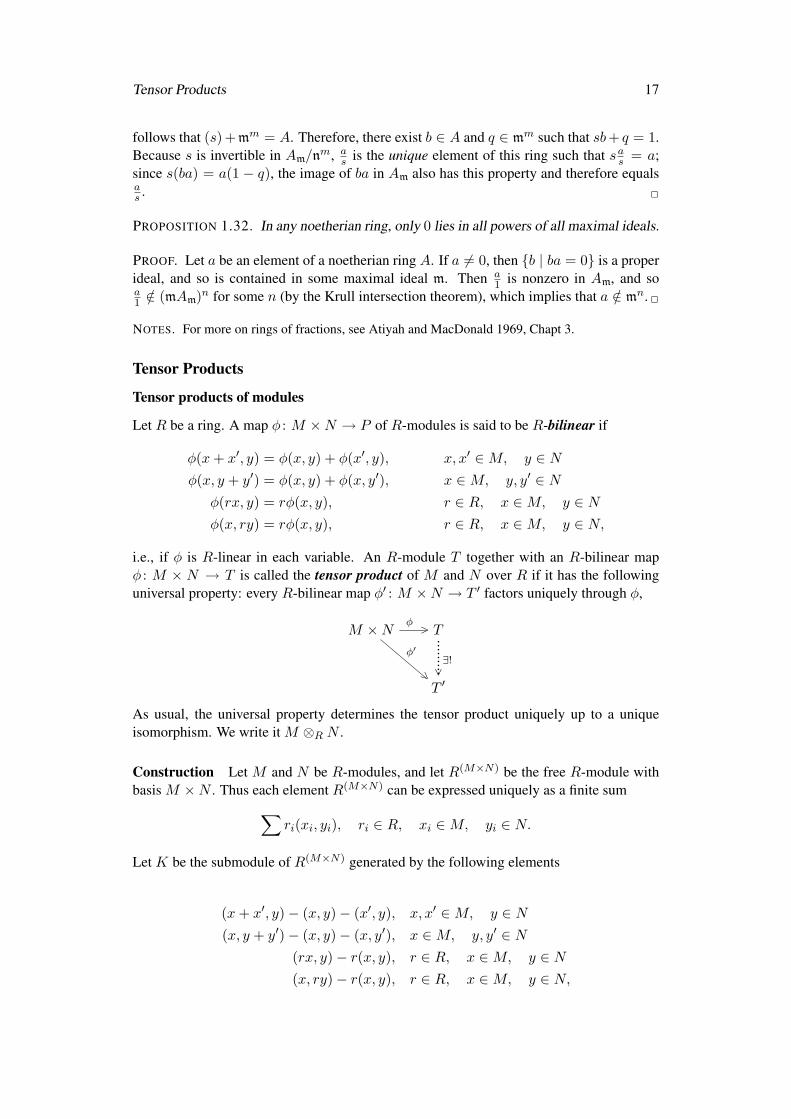
i.e., if φ is R-linear in each variable. An R-module T together with an R-bilinear mapφ : M × N → T is called the tensor product of M and N over R if it has the followinguniversal property: every R-bilinear map φ′ : M ×N → T ′ factors uniquely through φ,

M ×N φ> T

T ′

∃!∨

.........φ′

>

As usual, the universal property determines the tensor product uniquely up to a uniqueisomorphism. We write it M ⊗R N .

Construction Let M and N be R-modules, and let R(M×N) be the free R-module withbasis M ×N . Thus each element R(M×N) can be expressed uniquely as a finite sum∑

ri(xi, yi), ri ∈ R, xi ∈M, yi ∈ N.

Let K be the submodule of R(M×N) generated by the following elements

(x+ x′, y)− (x, y)− (x′, y), x, x′ ∈M, y ∈ N(x, y + y′)− (x, y)− (x, y′), x ∈M, y, y′ ∈ N

(rx, y)− r(x, y), r ∈ R, x ∈M, y ∈ N(x, ry)− r(x, y), r ∈ R, x ∈M, y ∈ N,

18 1 PRELIMINARIES

and defineM ⊗R N = R(M×N)/K.

Write x⊗ y for the class of (x, y) in M ⊗R N . Then

(x, y) 7→ x⊗ y : M ×N →M ⊗R N

is R-bilinear — we have imposed the fewest relations necessary to ensure this. Everyelement of M ⊗R N can be written as a finite sum∑

ri(xi ⊗ yi), ri ∈ R, xi ∈M, yi ∈ N,

and all relations among these symbols are generated by the following

(x+ x′)⊗ y = x⊗ y + x′ ⊗ yx⊗ (y + y′) = x⊗ y + x⊗ y′

r(x⊗ y) = (rx)⊗ y = x⊗ ry.

The pair (M ⊗R N, (x, y) 7→ x⊗ y) has the following universal property:

Tensor products of algebras

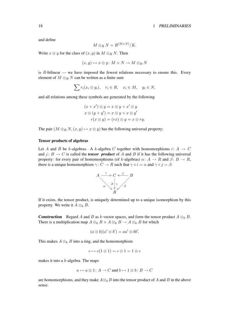
Let A and B be k-algebras. A k-algebra C together with homomorphisms i : A → Cand j : B → C is called the tensor product of A and B if it has the following universalproperty: for every pair of homomorphisms (of k-algebras) α : A → R and β : B → R,there is a unique homomorphism γ : C → R such that γ i = α and γ j = β:

Ai> C <

jB

R

∃! γ

∨

......... β<

α >

If it exists, the tensor product, is uniquely determined up to a unique isomorphism by thisproperty. We write it A⊗k B.

Construction Regard A and B as k-vector spaces, and form the tensor product A⊗k B.There is a multiplication map A⊗k B ×A⊗k B → A⊗k B for which

(a⊗ b)(a′ ⊗ b′) = aa′ ⊗ bb′.

This makes A⊗k B into a ring, and the homomorphism

c 7→ c(1⊗ 1) = c⊗ 1 = 1⊗ c

makes it into a k-algebra. The maps

a 7→ a⊗ 1: A→ C and b 7→ 1⊗ b : B → C

are homomorphisms, and they makeA⊗kB into the tensor product ofA andB in the abovesense.

Tensor Products 19

EXAMPLE 1.33. The algebra B, together with the given map k → B and the identity mapB → B, has the universal property characterizing k ⊗k B. In terms of the constructivedefinition of tensor products, the map c⊗ b 7→ cb : k ⊗k B → B is an isomorphism.

EXAMPLE 1.34. The ring k[X1, . . . , Xm, Xm+1, . . . , Xm+n], together with the obviousinclusions

k[X1, . . . , Xm] ⊂ > k[X1, . . . , Xm+n] < ⊃ k[Xm+1, . . . , Xm+n]

is the tensor product of k[X1, . . . , Xm] and k[Xm+1, . . . , Xm+n]. To verify this we onlyhave to check that, for every k-algebra R, the map

Homk-alg(k[X1, . . . , Xm+n], R)→ Homk-alg(k[X1, . . .], R)×Homk-alg(k[Xm+1, . . .], R)

induced by the inclusions is a bijection. But this map can be identified with the bijection

Rm+n → Rm ×Rn.

In terms of the constructive definition of tensor products, the map

f ⊗ g 7→ fg : k[X1, . . . , Xm]⊗k k[Xm+1, . . . , Xm+n]→ k[X1, . . . , Xm+n]

is an isomorphism.

REMARK 1.35. (a) If (bα) is a family of generators (resp. basis) for B as a k-vector space,then (1⊗ bα) is a family of generators (resp. basis) for A⊗k B as an A-module.

(b) Let k → Ω be fields. Then

Ω⊗k k[X1, . . . , Xn] ' Ω[1⊗X1, . . . , 1⊗Xn] ' Ω[X1, . . . , Xn].

If A = k[X1, . . . , Xn]/(g1, . . . , gm), then

Ω⊗k A ' Ω[X1, . . . , Xn]/(g1, . . . , gm).

(c) If A and B are algebras of k-valued functions on sets S and T respectively, then(f ⊗ g)(x, y) = f(x)g(y) realizes A⊗k B as an algebra of k-valued functions on S × T .

For more details on tensor products, see Atiyah and MacDonald 1969, Chapter 2 (butnote that the description there (p31) of the homomorphism A → D making the tensorproduct into an A-algebra is incorrect — the map is a 7→ f(a)⊗ 1 = 1⊗ g(a).)

Extension of scalars

Let R be a commutative ring and A an R-algebra (not necessarily commutative) such thatthe image of R → A lies in the centre of A. Then we have a functor M 7→ A⊗RM fromleft R-modules to left A-modules.

Behaviour with respect to direct limits

PROPOSITION 1.36. Direct limits commute with tensor products:

lim−→i∈I

Mi ⊗R lim−→j∈J

Nj ' lim−→(i,j)∈I×J

(Mi ⊗R Nj).

PROOF. Using the universal properties of direct limits and tensor products, one sees easilythat lim−→(Mi ⊗R Nj) has the universal property to be the tensor product of lim−→Mi andlim−→Nj . 2

20 1 PRELIMINARIES

Flatness

For any R-module M , the functor N 7→M ⊗R N is right exact, i.e.,

M ⊗R N ′ →M ⊗R N →M ⊗R N ′′ → 0

is exact wheneverN ′ → N → N ′′ → 0

is exact. If M ⊗R N → M ⊗R N ′ is injective whenever N → N ′ is injective, then M issaid to be flat. Thus M is flat if and only if the functor N 7→ M ⊗R N is exact. Similarly,an R-algebra A is flat if N 7→ A⊗R N is flat.

PROPOSITION 1.37. To be added.

Categories and functors

A category C consists of(a) a class of objects ob(C);(b) for each pair (a, b) of objects, a set Mor(a, b), whose elements are called morphisms

from a to b, and are written α : a→ b;(c) for each triple of objects (a, b, c) a map (called composition)

(α, β) 7→ β α : Mor(a, b)×Mor(b, c)→ Mor(a, c).

Composition is required to be associative, i.e., (γ β)α = γ (β α), and for each objecta there is required to be an element ida ∈ Mor(a, a) such that ida α = α, β ida = β, forall α and β for which these composites are defined. The sets Mor(a, b) are required to bedisjoint (so that a morphism α determines its source and target).

EXAMPLE 1.38. (a) There is a category of sets, Sets, whose objects are the sets and whosemorphisms are the usual maps of sets.

(b) There is a category Affk of affine k-algebras, whose objects are the affine k-algebrasand whose morphisms are the homomorphisms of k-algebras.

(c) In Section 4 below, we define a category Vark of algebraic varieties over k, whoseobjects are the algebraic varieties over k and whose morphisms are the regular maps.

The objects in a category need not be sets with structure, and the morphisms need notbe maps.

Let C and D be categories. A covariant functor F from C to D consists of(a) a map a 7→ F (a) sending each object of C to an object of D, and,(b) for each pair of objects a, b of C, a map

α 7→ F (α) : Mor(a, b)→ Mor(F (a), F (b))

such that F (idA) = idF (A) and F (β α) = F (β) F (α).A contravariant functor is defined similarly, except that the map on morphisms is

α 7→ F (α) : Mor(a, b)→ Mor(F (b), F (a))

A functor F : C→ D is full (resp. faithful, fully faithful) if, for all objects a and b ofC, the map

Mor(a, b)→ Mor(F (a), F (b))

Categories and functors 21

is a surjective (resp. injective, bijective).A covariant functor F : A→ B of categories is said to be an equivalence of categories

if it is fully faithful and every object of B is isomorphic to an object of the form F (a),a ∈ ob(A) (F is essentially surjective). One can show that such a functor F has a quasi-inverse, i.e., that there is a functor G : B→ A, which is also an equivalence, and for whichthere exist natural isomorphisms G(F (A)) ≈ A and F (G(B)) ≈ B. Hence the relation ofequivalence is an equivalence relation. (In fact one can do better — see Bucur and Deleanu19689, I 6, or Mac Lane 199810, IV 4.)

Similarly one defines the notion of a contravariant functor being an equivalence of cat-egories.

Any fully faithful functor F : C → D defines an equivalence of C with the full subcat-egory of D whose objects are isomorphic to F (a) for some object a of C. The essentialimage of a fully faithful functor F : C → D consists of the objects of D isomorphic to anobject of the form F (a), a ∈ ob(C).

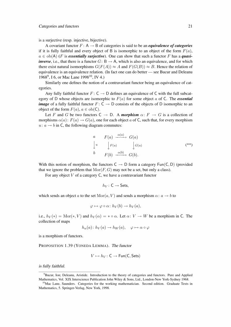
Let F and G be two functors C → D. A morphism α : F → G is a collection ofmorphisms α(a) : F (a)→ G(a), one for each object a of C, such that, for every morphismu : a→ b in C, the following diagram commutes:

ayub

F (a)α(a)−−−−→ G(a)yF (u)

yG(u)

F (b)α(b)−−−−→ G(b).

(**)

With this notion of morphism, the functors C → D form a category Fun(C,D) (providedthat we ignore the problem that Mor(F,G) may not be a set, but only a class).

For any object V of a category C, we have a contravariant functor

hV : C→ Sets,

which sends an object a to the set Mor(a, V ) and sends a morphism α : a→ b to

ϕ 7→ ϕ α : hV (b)→ hV (a),

i.e., hV (∗) = Mor(∗, V ) and hV (α) = ∗ α. Let α : V → W be a morphism in C. Thecollection of maps

hα(a) : hV (a)→ hW (a), ϕ 7→ α ϕ

is a morphism of functors.

PROPOSITION 1.39 (YONEDA LEMMA). The functor

V 7→ hV : C→ Fun(C,Sets)

is fully faithful.

9Bucur, Ion; Deleanu, Aristide. Introduction to the theory of categories and functors. Pure and AppliedMathematics, Vol. XIX Interscience Publication John Wiley & Sons, Ltd., London-New York-Sydney 1968.

10Mac Lane, Saunders. Categories for the working mathematician. Second edition. Graduate Texts inMathematics, 5. Springer-Verlag, New York, 1998.

22 1 PRELIMINARIES

PROOF. Let a, b be objects of C. We construct an inverse to

α 7→ hα : Mor(a, b)→ Mor(ha, hb).

A morphism of functors γ : ha → ha defines a map γ(a) : ha(a) → ha(b), and we letβ(γ) = γ(ida) — it is morphism a→ b. Then

β(hα) df= hα(ida)df= α ida = α,

andhβ(γ)(α) df= β(γ) α df= γ(idA) α = γ(α)

because of the commutativity of (**):

a ha(a)γ> hb(a)

b

α

∨hb(b)

∗α∨

γ> hb(b)

∗α∨

(***)

Thus α→ hα and γ 7→ β(γ) are inverse maps. 2

Algorithms for polynomialsAs an introduction to algorithmic algebraic geometry, we derive some algorithms for working withpolynomial rings. This subsection is little more than a summary of the first two chapters of Cox etal.1992 to which I refer the reader for more details. Those not interested in algorithms can skip theremainder of this section. Throughout, k is a field (not necessarily algebraically closed).

The two main results will be:(a) An algorithmic proof of the Hilbert basis theorem: every ideal in k[X1, . . . , Xn] has a finite

set of generators (in fact, of a special kind).(b) There exists an algorithm for deciding whether a polynomial belongs to an ideal.

Division in k[X]

The division algorithm allows us to divide a nonzero polynomial into another: let f and g be poly-nomials in k[X] with g 6= 0; then there exist unique polynomials q, r ∈ k[X] such that f = qg + rwith either r = 0 or deg r < deg g. Moreover, there is an algorithm for deciding whether f ∈ (g),namely, find r and check whether it is zero.

In Maple,quo(f, g, X); computes qrem(f, g, X); computes r

Moreover, the Euclidean algorithm allows you to pass from a finite set of generators for an idealin k[X] to a single generator by successively replacing each pair of generators with their greatestcommon divisor.

Orderings on monomials

Before we can describe an algorithm for dividing in k[X1, . . . , Xn], we shall need to choose a wayof ordering monomials. Essentially this amounts to defining an ordering on Nn. There are two mainsystems, the first of which is preferred by humans, and the second by machines.

(Pure) lexicographic ordering (lex). Here monomials are ordered by lexicographic (dictionary)order. More precisely, let α = (a1, . . . , an) and β = (b1, . . . , bn) be two elements of Nn; then

α > β and Xα > Xβ (lexicographic ordering)

Algorithms for polynomials 23

if, in the vector difference α − β (an element of Zn), the left-most nonzero entry is positive. Forexample,

XY 2 > Y 3Z4; X3Y 2Z4 > X3Y 2Z.

Note that this isn’t quite how the dictionary would order them: it would put XXXYYZZZZ afterXXXYYZ.

Graded reverse lexicographic order (grevlex). Here monomials are ordered by total degree,with ties broken by reverse lexicographic ordering. Thus, α > β if

∑ai >

∑bi, or

∑ai =

∑bi

and in α− β the right-most nonzero entry is negative. For example:

X4Y 4Z7 > X5Y 5Z4 (total degree greater)

XY 5Z2 > X4Y Z3, X5Y Z > X4Y Z2.

Orderings on k[X1, . . . , Xn]

Fix an ordering on the monomials in k[X1, . . . , Xn]. Then we can write an element f of k[X1, . . . , Xn]in a canonical fashion by re-ordering its elements in decreasing order. For example, we would write

f = 4XY 2Z + 4Z2 − 5X3 + 7X2Z2

asf = −5X3 + 7X2Z2 + 4XY 2Z + 4Z2 (lex)

orf = 4XY 2Z + 7X2Z2 − 5X3 + 4Z2 (grevlex)

Let f =∑aαX

α ∈ k[X1, . . . , Xn]. Write it in decreasing order:

f = aα0Xα0 + aα1X

α1 + · · · , α0 > α1 > · · · , aα0 6= 0.

Then we define:(a) the multidegree of f to be multdeg(f) = α0;(b) the leading coefficient of f to be LC(f) = aα0 ;(c) the leading monomial of f to be LM(f) = Xα0 ;(d) the leading term of f to be LT(f) = aα0X

α0 .For example, for the polynomial f = 4XY 2Z + · · · , the multidegree is (1, 2, 1), the leading coeffi-cient is 4, the leading monomial is XY 2Z, and the leading term is 4XY 2Z.

The division algorithm in k[X1, . . . , Xn]

Fix a monomial ordering in Nn. Suppose given a polynomial f and an ordered set (g1, . . . , gs) ofpolynomials; the division algorithm then constructs polynomials a1, . . . , as and r such that

f = a1g1 + · · ·+ asgs + r

where either r = 0 or no monomial in r is divisible by any of LT(g1), . . . ,LT(gs).STEP 1: If LT(g1)|LT(f), divide g1 into f to get

f = a1g1 + h, a1 =LT(f)LT(g1)

∈ k[X1, . . . , Xn].

If LT(g1)|LT(h), repeat the process until

f = a1g1 + f1

(different a1) with LT(f1) not divisible by LT(g1). Now divide g2 into f1, and so on, until

f = a1g1 + · · ·+ asgs + r1

24 1 PRELIMINARIES

with LT(r1) not divisible by any of LT(g1), . . . , LT(gs).STEP 2: Rewrite r1 = LT(r1) + r2, and repeat Step 1 with r2 for f :

f = a1g1 + · · ·+ asgs + LT(r1) + r3

(different ai’s).STEP 3: Rewrite r3 = LT(r3) + r4, and repeat Step 1 with r4 for f :

f = a1g1 + · · ·+ asgs + LT(r1) + LT(r3) + r3

(different ai’s).Continue until you achieve a remainder with the required property. In more detail,11 after di-

viding through once by g1, . . . , gs, you repeat the process until no leading term of one of the gi’sdivides the leading term of the remainder. Then you discard the leading term of the remainder, andrepeat.

EXAMPLE 1.40. (a) Consider

f = X2Y +XY 2 + Y 2, g1 = XY − 1, g2 = Y 2 − 1.

First, on dividing g1 into f , we obtain

X2Y +XY 2 + Y 2 = (X + Y )(XY − 1) +X + Y 2 + Y.

This completes the first step, because the leading term of Y 2− 1 does not divide the leading term ofthe remainder X + Y 2 + Y . We discard X , and write

Y 2 + Y = 1 · (Y 2 − 1) + Y + 1.

Altogether

X2Y +XY 2 + Y 2 = (X + Y ) · (XY − 1) + 1 · (Y 2 − 1) +X + Y + 1.

(b) Consider the same polynomials, but with a different order for the divisors

f = X2Y +XY 2 + Y 2, g1 = Y 2 − 1, g2 = XY − 1.

In the first step,

X2Y +XY 2 + Y 2 = (X + 1) · (Y 2 − 1) +X · (XY − 1) + 2X + 1.

Thus, in this case, the remainder is 2X + 1.

REMARK 1.41. If r = 0, then f ∈ (g1, . . . , gs), but, because the remainder depends on the orderingof the gi, the converse is false. For example, (lex ordering)

XY 2 −X = Y · (XY + 1) + 0 · (Y 2 − 1) +−X − Y

butXY 2 −X = X · (Y 2 − 1) + 0 · (XY + 1) + 0.

Thus, the division algorithm (as stated) will not provide a test for f lying in the ideal generated byg1, . . . , gs.

11This differs from the algorithm in Cox et al. 1992, p63, which says to go back to g1 after every successfuldivision.

Algorithms for polynomials 25

Monomial ideals

In general, an ideal a can contain a polynomial without containing the individual monomials of thepolynomial; for example, the ideal a = (Y 2 −X3) contains Y 2 −X3 but not Y 2 or X3.

DEFINITION 1.42. An ideal a is monomial if∑cαX

α ∈ a and cα 6= 0 =⇒ Xα ∈ a.

PROPOSITION 1.43. Let a be a monomial ideal, and let A = α | Xα ∈ a. Then A satisfies thecondition

α ∈ A, β ∈ Nn =⇒ α+ β ∈ A (*)

and a is the k-subspace of k[X1, . . . , Xn] generated by the Xα, α ∈ A. Conversely, if A is a subsetof Nn satisfying (*), then the k-subspace a of k[X1, . . . , Xn] generated by Xα | α ∈ A is amonomial ideal.

PROOF. It is clear from its definition that a monomial ideal a is the k-subspace of k[X1, . . . , Xn]generated by the set of monomials it contains. If Xα ∈ a and Xβ ∈ k[X1, . . . , Xn], then XαXβ =Xα+β ∈ a, and so A satisfies the condition (*). Conversely,(∑

α∈A

cαXα

)∑β∈Nn

dβXβ

=∑α,β

cαdβXα+β (finite sums),

and so if A satisfies (*), then the subspace generated by the monomials Xα, α ∈ A, is an ideal. 2

The proposition gives a classification of the monomial ideals in k[X1, . . . , Xn]: they are in one-to-one correspondence with the subsets A of Nn satisfying (*). For example, the monomial idealsin k[X] are exactly the ideals (Xn), n ≥ 0, and the zero ideal (corresponding to the empty set A).We write

〈Xα | α ∈ A〉

for the ideal corresponding to A (subspace generated by the Xα, α ∈ A).

LEMMA 1.44. Let S be a subset of Nn. Then the ideal a generated by Xα | α ∈ S is themonomial ideal corresponding to

Adf= β ∈ Nn | β − α ∈ S, some α ∈ S.

In other words, a monomial is in a if and only if it is divisible by one of the Xα, α ∈ S.

PROOF. Clearly A satisfies (*), and a ⊂ 〈Xβ | β ∈ A〉. Conversely, if β ∈ A, then β−α ∈ Nn forsome α ∈ S, and Xβ = XαXβ−α ∈ a. The last statement follows from the fact that Xα|Xβ ⇐⇒β − α ∈ Nn. 2

Let A ⊂ N2 satisfy (*). From the geometry of A, it is clear that there is a finite set of elementsS = α1, . . . , αs of A such that

A = β ∈ N2 | β − αi ∈ N2, some αi ∈ S.

(The αi’s are the “corners” of A.) Moreover, the ideal 〈Xα | α ∈ A〉 is generated by the monomialsXαi , αi ∈ S. This suggests the following result.

THEOREM 1.45 (DICKSON’S LEMMA). Let a be the monomial ideal corresponding to the subsetA ⊂ Nn. Then a is generated by a finite subset of Xα | α ∈ A.

PROOF. This is proved by induction on the number of variables — Cox et al. 1992, p70. 2

26 1 PRELIMINARIES

Hilbert Basis Theorem

DEFINITION 1.46. For a nonzero ideal a in k[X1, . . . , Xn], we let (LT(a)) be the ideal generatedby LT(f) | f ∈ a.

LEMMA 1.47. Let a be a nonzero ideal in k[X1, . . . , Xn]; then (LT(a)) is a monomial ideal, and itequals (LT(g1), . . . ,LT(gn)) for some g1, . . . , gn ∈ a.

PROOF. Since (LT(a)) can also be described as the ideal generated by the leading monomials (ratherthan the leading terms) of elements of a, it follows from Lemma 1.44 that it is monomial. NowDickson’s Lemma shows that it equals (LT(g1), . . . ,LT(gs)) for some gi ∈ a. 2

THEOREM 1.48 (HILBERT BASIS THEOREM). Every ideal a in k[X1, . . . , Xn] is finitely gener-ated; in fact, a is generated by any elements of a whose leading terms generate LT(a).

PROOF. Let g1, . . . , gn be as in the lemma, and let f ∈ a. On applying the division algorithm, wefind

f = a1g1 + · · ·+ asgs + r, ai, r ∈ k[X1, . . . , Xn],

where either r = 0 or no monomial occurring in it is divisible by any LT(gi). But r = f −∑aigi ∈

a, and therefore LT(r) ∈ LT(a) = (LT(g1), . . . ,LT(gs)), which, according to Lemma 1.44, impliesthat every monomial occurring in r is divisible by one in LT(gi). Thus r = 0, and g ∈ (g1, . . . , gs).2

Standard (Grobner) bases

Fix a monomial ordering of k[X1, . . . , Xn].

DEFINITION 1.49. A finite subset S = g1, . . . , gs of an ideal a is a standard (Grobner, Groeb-ner, Grobner) basis12 for a if

(LT(g1), . . . ,LT(gs)) = LT(a).

In other words, S is a standard basis if the leading term of every element of a is divisible by at leastone of the leading terms of the gi.

THEOREM 1.50. Every ideal has a standard basis, and it generates the ideal; if g1, . . . , gs is astandard basis for an ideal a, then f ∈ a ⇐⇒ the remainder on division by the gi is 0.

PROOF. Our proof of the Hilbert basis theorem shows that every ideal has a standard basis, andthat it generates the ideal. Let f ∈ a. The argument in the same proof, that the remainder of f ondivision by g1, . . . , gs is 0, used only that g1, . . . , gs is a standard basis for a. 2

REMARK 1.51. The proposition shows that, for f ∈ a, the remainder of f on division by g1, . . . , gsis independent of the order of the gi (in fact, it’s always zero). This is not true if f /∈ a — see theexample using Maple at the end of this section.

Let a = (f1, . . . , fs). Typically, f1, . . . , fs will fail to be a standard basis because in someexpression

cXαfi − dXβfj , c, d ∈ k, (**)

the leading terms will cancel, and we will get a new leading term not in the ideal generated by theleading terms of the fi. For example,

X2 = X · (X2Y +X − 2Y 2)− Y · (X3 − 2XY )

12Standard bases were first introduced (under that name) by Hironaka in the mid-1960s, and independently,but slightly later, by Buchberger in his Ph.D. thesis. Buchberger named them after his thesis adviser Grobner.

Algorithms for polynomials 27

is in the ideal generated by X2Y +X − 2Y 2 and X3 − 2XY but it is not in the ideal generated bytheir leading terms.

There is an algorithm for transforming a set of generators for an ideal into a standard basis,which, roughly speaking, makes adroit use of equations of the form (**) to construct enough newelements to make a standard basis — see Cox et al. 1992, pp80–87.

We now have an algorithm for deciding whether f ∈ (f1, . . . , fr). First transform f1, . . . , frinto a standard basis g1, . . . , gs, and then divide f by g1, . . . , gs to see whether the remainder is0 (in which case f lies in the ideal) or nonzero (and it doesn’t). This algorithm is implemented inMaple — see below.

A standard basis g1, . . . , gs is minimal if each gi has leading coefficient 1 and, for all i, theleading term of gi does not belong to the ideal generated by the leading terms of the remaining g’s.A standard basis g1, . . . , gs is reduced if each gi has leading coefficient 1 and if, for all i, nomonomial of gi lies in the ideal generated by the leading terms of the remaining g’s. One can prove(Cox et al. 1992, p91) that every nonzero ideal has a unique reduced standard basis.

REMARK 1.52. Consider polynomials f, g1, . . . , gs ∈ k[X1, . . . , Xn]. The algorithm that replacesg1, . . . , gs with a standard basis works entirely within k[X1, . . . , Xn], i.e., it doesn’t require a fieldextension. Likewise, the division algorithm doesn’t require a field extension. Because these opera-tions give well-defined answers, whether we carry them out in k[X1, . . . , Xn] or in K[X1, . . . , Xn],K ⊃ k, we get the same answer. Maple appears to work in the subfield of C generated over Q byall the constants occurring in the polynomials.

We conclude this section with the annotated transcript of a session in Maple applying the abovealgorithm to show that

q = 3x3yz2 − xz2 + y3 + yz

doesn’t lie in the ideal(x2 − 2xz + 5, xy2 + yz3, 3y2 − 8z3).

A Maple session>with(grobner):

This loads the grobner package, and lists the available commands:finduni, finite, gbasis, gsolve, leadmon, normalf, solvable, spoly

To discover the syntax of a command, a brief description of the command, and an example, type“?command;”

>G:=gbasis([xˆ2-2*x*z+5,x*yˆ2+y*zˆ3,3*yˆ2-8*zˆ3],[x,y,z]);G := [x2 − 2xz + 5,−3y2 + 8z3, 8xy2 + 3y3, 9y4 + 48zy3 + 320y2]

This asks Maple to find the reduced Grobner basis for the ideal generated by the three polynomialslisted, with respect to the symbols listed (in that order). It will automatically use grevlex order unlessyou add ,plex to the command.

> q:=3*xˆ3*y*zˆ2 - x*zˆ2 + yˆ3 + y*z;q := 3x3yz2 − xz2 + y3 + zy

This defines the polynomial q.> normalf(q,G,[x,y,z]);9z2y3 − 15yz2x− 41

4 y3 + 60y2z − xz2 + zy

Asks for the remainder when q is divided by the polynomials listed in G using the symbols listed.This particular example is amusing — the program gives different orderings for G, and differentanswers for the remainder, depending on which computer I use. This is O.K., because, since q isn’tin the ideal, the remainder may depend on the ordering of G.

Notes:

(a) To start Maple on a Unix computer type “maple”; to quit type “quit”.(b) Maple won’t do anything until you type “;” or “:” at the end of a line.(c) The student version of Maple is quite cheap, but unfortunately, it doesn’t have the Grobner

package.

28 1 PRELIMINARIES

(d) For more information on Maple:i) There is a brief discussion of the Grobner package in Cox et al. 1992, Appendix C, §1.

ii) The Maple V Library Reference Manual pp469–478 briefly describes what the Grobnerpackage does (exactly the same information is available on line, by typing ?command).

iii) There are many books containing general introductions to Maple syntax.(e) Grobner bases are also implemented in Macsyma, Mathematica, and Axiom, but for serious

work it is better to use one of the programs especially designed for Grobner basis computa-tion, namely,CoCoA (Computations in Commutative Algebra) http://cocoa.dima.unige.it/.Macaulay 2 (Grayson and Stillman) http://www.math.uiuc.edu/Macaulay2/.

Exercises

1-1. Let k be an infinite field (not necessarily algebraically closed). Show that an f ∈k[X1, . . . , Xn] that is identically zero on kn is the zero polynomial (i.e., has all its coeffi-cients zero).

1-2. Find a minimal set of generators for the ideal

(X + 2Y, 3X + 6Y + 3Z, 2X + 4Y + 3Z)

in k[X,Y, Z]. What standard algorithm in linear algebra will allow you to answer thisquestion for any ideal generated by homogeneous linear polynomials? Find a minimal setof generators for the ideal

(X + 2Y + 1, 3X + 6Y + 3X + 2, 2X + 4Y + 3Z + 3).

29

2 Algebraic Sets

In this section, k is an algebraically closed field.

Definition of an algebraic set

An algebraic subset V (S) of kn is the set of common zeros of some set S of polynomialsin k[X1, . . . , Xn]:

V (S) = (a1, . . . , an) ∈ kn | f(a1, . . . , an) = 0 all f(X1, . . . , Xn) ∈ S.

Note thatS ⊂ S′ =⇒ V (S) ⊃ V (S′);

— more equations means fewer solutions.Recall that the ideal a generated by a set S consists of all finite sums∑

figi, fi ∈ k[X1, . . . , Xn], gi ∈ S.

Such a sum∑figi is zero at any point at which the gi are all zero, and so V (S) ⊂ V (a),

but the reverse conclusion is also true because S ⊂ a. Thus V (S) = V (a) — the zero setof S is the same as that of the ideal generated by S. Hence the algebraic sets can also bedescribed as the sets of the form V (a), a an ideal in k[X1, . . . , Xn].

EXAMPLE 2.1. (a) If S is a system of homogeneous linear equations, then V (S) is a sub-space of kn. If S is a system of nonhomogeneous linear equations, then V (S) is eitherempty or is the translate of a subspace of kn.

(b) If S consists of the single equation

Y 2 = X3 + aX + b, 4a3 + 27b2 6= 0,

then V (S) is an elliptic curve. For more on elliptic curves, and their relation to Fermat’s lasttheorem, see my notes on Elliptic Curves. The reader should sketch the curve for particularvalues of a and b. We generally visualize algebraic sets as though the field k were R,although this can be misleading.

(c) For the empty set ∅, V (∅) = kn.(d) The algebraic subsets of k are the finite subsets (including ∅) and k itself.(e) Some generating sets for an ideal will be more useful than others for determining

what the algebraic set is. For example, a Grobner basis for the ideal

a = (X2 + Y 2 + Z2 − 1, X2 + Y 2 − Y, X − Z)

is (according to Maple)

X − Z, Y 2 − 2Y + 1, Z2 − 1 + Y.

The middle polynomial has (double) root 1, and it follows easily that V (a) consists of thesingle point (0, 1, 0).

30 2 ALGEBRAIC SETS

The Hilbert basis theorem

In our definition of an algebraic set, we didn’t require the set S of polynomials to be fi-nite, but the Hilbert basis theorem shows that every algebraic set will also be the zeroset of a finite set of polynomials. More precisely, the theorem shows that every ideal ink[X1, . . . , Xn] can be generated by a finite set of elements, and we have already observedthat any set of generators of an ideal has the same zero set as the ideal.

We sketched an algorithmic proof of the Hilbert basis theorem in the last section. Herewe give the slick proof.

THEOREM 2.2 (HILBERT BASIS THEOREM). The ring k[X1, . . . , Xn] is noetherian, i.e.,every ideal is finitely generated.

Since k itself is noetherian, and k[X1, . . . , Xn−1][Xn] = k[X1, . . . , Xn], the theoremfollows by induction from the next lemma.

LEMMA 2.3. If A is noetherian, then so also is A[X].

PROOF. Recall that for a polynomial

f(X) = a0Xr + a1X

r−1 + · · ·+ ar, ai ∈ A, a0 6= 0,

r is called the degree of f , and a0 is its leading coefficient.Let a be an ideal inA[X], and let ai be the set of elements ofA that occur as the leading

coefficient of a polynomial in a of degree ≤ i. Then ai is an ideal in A, and

a1 ⊂ a2 ⊂ · · · ⊂ ai ⊂ · · · .

Because A is noetherian, this sequence eventually becomes constant, say ad = ad+1 = . . .(and ad consists of the leading coefficients of all polynomials in a).

For each i ≤ d, choose a finite set fi1, fi2, . . . of polynomials in a of degree i such thatthe leading coefficients aij of the fij’s generate ai.

Let f ∈ a; we shall prove by induction on the degree of f that it lies in the idealgenerated by the fij . When f has degree 1, this is clear.

Suppose that f has degree s ≥ d. Then f = aXs + · · · with a ∈ ad, and so

a =∑

jbjadj , some bj ∈ A.

Nowf −

∑jbjfdjX

s−d

has degree < deg(f), and so lies in (fij).Suppose that f has degree s ≤ r. Then a similar argument shows that

f −∑

bjfsj

has degree < deg(f) for suitable bj ∈ A, and so lies in (fij). 2

ASIDE 2.4. One may ask how many elements are needed to generate a given ideal a ink[X1, . . . , Xn], or, what is not quite the same thing, how many equations are needed todefine a given algebraic set V . When n = 1, we know that every ideal is generated by asingle element. Also, if V is a linear subspace of kn, then linear algebra shows that it is thezero set of n−dim(V ) polynomials. All one can say in general, is that at least n−dim(V )polynomials are needed to define V (see 9.7), but often more are required. Determiningexactly how many is an area of active research — see (9.14).

The Zariski topology 31

The Zariski topology

PROPOSITION 2.5. There are the following relations:(a) a ⊂ b =⇒ V (a) ⊃ V (b);(b) V (0) = kn; V (k[X1, . . . , Xn]) = ∅;(c) V (ab) = V (a ∩ b) = V (a) ∪ V (b);(d) V (

∑i∈I ai) =

⋂i∈I V (ai) for any family of ideals (ai)i∈I .

PROOF. The first two statements are obvious. For (c), note that

ab ⊂ a ∩ b ⊂ a, b =⇒ V (ab) ⊃ V (a ∩ b) ⊃ V (a) ∪ V (b).

For the reverse inclusions, observe that if a /∈ V (a) ∪ V (b), then there exist f ∈ a, g ∈ b

such that f(a) 6= 0, g(a) 6= 0; but then (fg)(a) 6= 0, and so a /∈ V (ab). For (d) recallthat, by definition,

∑ai consists of all finite sums of the form

∑fi, fi ∈ ai. Thus (d) is

obvious. 2

Statements (b), (c), and (d) show that the algebraic subsets of kn satisfy the axioms to bethe closed subsets for a topology on kn: both the whole space and the empty set are closed;a finite union of closed sets is closed; an arbitrary intersection of closed sets is closed. Thistopology is called the Zariski topology on kn. The induced topology on a subset V of kn iscalled the Zariski topology on V .

The Zariski topology has many strange properties, but it is nevertheless of great impor-tance. For the Zariski topology on k, the closed subsets are just the finite sets and the wholespace, and so the topology is not Hausdorff. We shall see in (2.29) below that the properclosed subsets of k2 are finite unions of (isolated) points and curves (zero sets of irreduciblef ∈ k[X,Y ]). Note that the Zariski topologies on C and C2 are much coarser (have manyfewer open sets) than the complex topologies.

The Hilbert Nullstellensatz

We wish to examine the relation between the algebraic subsets of kn and the ideals ofk[X1, . . . , Xn], but first we consider the question of when a set of polynomials has a com-mon zero, i.e., when the equations

g(X1, . . . , Xn) = 0, g ∈ a,

are “consistent”. Obviously, the equations

gi(X1, . . . , Xn) = 0, i = 1, . . . ,m

are inconsistent if there exist fi ∈ k[X1, . . . , Xn] such that∑figi = 1, i.e., if 1 ∈

(g1, . . . , gm) or, equivalently, (g1, . . . , gm) = k[X1, . . . , Xn]. The next theorem provides aconverse to this.

THEOREM 2.6 (HILBERT NULLSTELLENSATZ). 13 Every proper ideal a in k[X1, . . . , Xn]has a zero in kn.

13Nullstellensatz = zero-points-theorem.

32 2 ALGEBRAIC SETS

A point P = (a1, . . . , an) in kn defines a homomorphism “evaluate at P ”

k[X1, . . . , Xn]→ k, f(X1, . . . , Xn) 7→ f(a1, . . . , an),

whose kernel contains a ifP ∈ V (a). Conversely, from a homomorphismϕ : k[X1, . . . , Xn]→k of k-algebras whose kernel contains a, we obtain a point P in V (a), namely,

P = (ϕ(X1), . . . , ϕ(Xn)).

Thus, to prove the theorem, we have to show that there exists a k-algebra homomorphismk[X1, . . . , Xn]/a→ k.

Since every proper ideal is contained in a maximal ideal, it suffices to prove this for amaximal ideal m. Then K df= k[X1, . . . , Xn]/m is a field, and it is finitely generated as analgebra over k (with generators X1 + m, . . . , Xn + m). To complete the proof, we mustshow K = k. The next lemma accomplishes this.

Although we shall apply the lemma only in the case that k is algebraically closed, inorder to make the induction in its proof work, we need to allow arbitrary k’s in the statement.

LEMMA 2.7 (ZARISKI’S LEMMA). Let k ⊂ K be fields (k is not necessarily algebraicallyclosed). If K is finitely generated as an algebra over k, then K is algebraic over k. (HenceK = k if k is algebraically closed.)

PROOF. We shall prove this by induction on r, the minimum number of elements requiredto generate K as a k-algebra. The case r = 0 being trivial, we may suppose that K =k[x1, . . . , xr] with r ≥ 1. If K is not algebraic over k, then at least one xi, say x1, is notalgebraic over k. Then, k[x1] is a polynomial ring in one symbol over k, and its field offractions k(x1) is a subfield ofK. ClearlyK is generated as a k(x1)-algebra by x2, . . . , xr,and so the induction hypothesis implies that x2, . . . , xr are algebraic over k(x1). Accordingto (1.18), there exists a d ∈ k[x1] such that dxi is integral over k[x1] for all i ≥ 2. Letf ∈ K = k[x1, . . . , xr]. For a sufficiently large N , dNf ∈ k[x1, dx2, . . . , dxr], and sodNf is integral over k[x1] (1.16). When we apply this statement to an element f of k(x1),(1.21) shows that dNf ∈ k[x1]. Therefore, k(x1) =

⋃N d

−Nk[x1], but this is absurd,because k[x1] (' k[X]) has infinitely many distinct monic irreducible polynomials14 thatcan occur as denominators of elements of k(x1). 2

The correspondence between algebraic sets and ideals

For a subset W of kn, we write I(W ) for the set of polynomials that are zero on W :

I(W ) = f ∈ k[X1, . . . , Xn] | f(P ) = 0 all P ∈W.

Clearly, it is an ideal in k[X1, . . . , Xn]. There are the following relations:(a) V ⊂W =⇒ I(V ) ⊃ I(W );(b) I(∅) = k[X1, . . . , Xn]; I(kn) = 0;(c) I(

⋃Wi) =

⋂I(Wi).

14If k is infinite, then consider the polynomials X − a, and if k is finite, consider the minimum polynomialsof generators of the extension fields of k. Alternatively, and better, adapt Euclid’s proof that there are infinitelymany prime numbers.

The correspondence between algebraic sets and ideals 33

Only the statement I(kn) = 0 is (perhaps) not obvious. It says that, if a polynomial isnonzero (in the ring k[X1, . . . , Xn]), then it is nonzero at some point of kn. This is truewith k any infinite field (see Exercise 1-1). Alternatively, it follows from the strong HilbertNullstellensatz (cf. 2.14a below).

EXAMPLE 2.8. Let P be the point (a1, . . . , an). Clearly I(P ) ⊃ (X1−a1, . . . , Xn−an),but (X1−a1, . . . , Xn−an) is a maximal ideal, because “evaluation at (a1, . . . , an)” definesan isomorphism

k[X1, . . . , Xn]/(X1 − a1, . . . , Xn − an)→ k.

As I(P ) is a proper ideal, it must equal (X1 − a1, . . . , Xn − an).

PROPOSITION 2.9. For any subset W ⊂ kn, V I(W ) is the smallest algebraic subset of kn

containing W . In particular, V I(W ) = W if W is an algebraic set.

PROOF. Let V be an algebraic set containing W , and write V = V (a). Then a ⊂ I(W ),and so V (a) ⊃ V I(W ). 2

The radical rad(a) of an ideal a is defined to be

f | f r ∈ a, some r ∈ N, r > 0.

PROPOSITION 2.10. Let a be an ideal in a ring A.(a) The radical of a is an ideal.(b) rad(rad(a)) = rad(a).

PROOF. (a) If a ∈ rad(a), then clearly fa ∈ rad(a) for all f ∈ A. Suppose a, b ∈ rad(a),with say ar ∈ a and bs ∈ a. When we expand (a + b)r+s using the binomial theorem, wefind that every term has a factor ar or bs, and so lies in a.

(b) If ar ∈ rad(a), then ars = (ar)s ∈ a for some s. 2

An ideal is said to be radical if it equals its radical, i.e., if f r ∈ a =⇒ f ∈ a.Equivalently, a is radical if and only if A/a is a reduced ring, i.e., a ring without nonzeronilpotent elements (elements some power of which is zero). Since integral domains arereduced, prime ideals (a fortiori maximal ideals) are radical.

If a and b are radical, then a∩b is radical, but a+b need not be: consider, for example,a = (X2 − Y ) and b = (X2 + Y ); they are both prime ideals in k[X,Y ], but X2 ∈ a + b,X /∈ a + b.

As f r(P ) = f(P )r, f r is zero wherever f is zero, and so I(W ) is radical. In particular,IV (a) ⊃ rad(a). The next theorem states that these two ideals are equal.

THEOREM 2.11 (STRONG HILBERT NULLSTELLENSATZ). For any ideal a in k[X1, . . . , Xn],IV (a) is the radical of a; in particular, IV (a) = a if a is a radical ideal.

PROOF. We have already noted that IV (a) ⊃ rad(a). For the reverse inclusion, we have toshow that if h is identically zero on V (a), then hN ∈ a for some N > 0. We may assumeh 6= 0. Let g1, . . . , gm generate a, and consider the system of m + 1 equations in n + 1variables, X1, . . . , Xn, Y,

gi(X1, . . . , Xn) = 0, i = 1, . . . ,m1− Y h(X1, . . . , Xn) = 0.

34 2 ALGEBRAIC SETS

If (a1, . . . , an, b) satisfies the first m equations, then (a1, . . . , an) ∈ V (a); consequently,h(a1, . . . , an) = 0, and (a1, . . . , an, b) doesn’t satisfy the last equation. Therefore, theequations are inconsistent, and so, according to the original Nullstellensatz, there existfi ∈ k[X1, . . . , Xn, Y ] such that

1 =m∑i=1

figi + fm+1 · (1− Y h)

(in the ring k[X1, . . . , Xn, Y ]). On regarding this as an identity in the ring k(X1, . . . , Xn)[Y ]and substituting15 h−1 for Y , we obtain the identity

1 =m∑i=1

fi(X1, . . . , Xn, h−1) · gi(X1, . . . , Xn) (*)

in k(X1, . . . , Xn). Clearly

fi(X1, . . . , Xn, h−1) =

polynomial in X1, . . . , Xn

hNi

for some Ni. Let N be the largest of the Ni. On multiplying (*) by hN we obtain anequation

hN =∑

(polynomial in X1, . . . , Xn) · gi(X1, . . . , Xn),

which shows that hN ∈ a. 2

COROLLARY 2.12. The map a 7→ V (a) defines a one-to-one correspondence between theset of radical ideals in k[X1, . . . , Xn] and the set of algebraic subsets of kn; its inverse is I .

PROOF. We know that IV (a) = a if a is a radical ideal (2.11), and that V I(W ) = W ifW is an algebraic set (2.9). Therefore, I and V are inverse maps. 2

COROLLARY 2.13. The radical of an ideal in k[X1, . . . , Xn] is equal to the intersection ofthe maximal ideals containing it.

PROOF. Let a be an ideal in k[X1, . . . , Xn]. Because maximal ideals are radical, everymaximal ideal containing a also contains rad(a):

rad(a) ⊂⋂m⊃a

m.

For each P = (a1, . . . , an) ∈ kn, mP = (X1− a1, . . . , Xn− an) is a maximal ideal ink[X1, . . . , Xn], and

f ∈ mP ⇐⇒ f(P ) = 0

(see 2.8). ThusmP ⊃ a ⇐⇒ P ∈ V (a).

If f ∈ mP for all P ∈ V (a), then f is zero on V (a), and so f ∈ IV (a) = rad(a). We haveshown that

rad(a) ⊃⋂

P∈V (a)

mP .

2

15More precisely, there is a homomorphism

Y 7→ h−1 : K[Y ] → K, K = k(X1, . . . , Xn),

which we apply to the identity.

Finding the radical of an ideal 35

REMARK 2.14. (a) Because V (0) = kn,

I(kn) = IV (0) = rad(0) = 0;

in other words, only the zero polynomial is zero on the whole of kn.(b) The one-to-one correspondence in the corollary is order inverting. Therefore the

maximal proper radical ideals correspond to the minimal nonempty algebraic sets. But themaximal proper radical ideals are simply the maximal ideals in k[X1, . . . , Xn], and theminimal nonempty algebraic sets are the one-point sets. As

I((a1, . . . , an)) = (X1 − a1, . . . , Xn − an)

(see 2.8), this shows that the maximal ideals of k[X1, . . . , Xn] are exactly the ideals of theform (X1 − a1, . . . , Xn − an).

(c) The algebraic set V (a) is empty if and only if a = k[X1, . . . , Xn], because

V (a) = ∅ ⇒ rad(a) = k[X1, . . . , Xn]⇒ 1 ∈ rad(a)⇒ 1 ∈ a.

(d) Let W and W ′ be algebraic sets. Then W ∩W ′ is the largest algebraic subset con-tained in both W and W ′, and so I(W ∩W ′) must be the smallest radical ideal containingboth I(W ) and I(W ′). Hence I(W ∩W ′) = rad(I(W ) + I(W ′)).

For example, let W = V (X2 − Y ) and W ′ = V (X2 + Y ); then I(W ∩ W ′) =rad(X2, Y ) = (X,Y ) (assuming characteristic 6= 2). Note that W ∩W ′ = (0, 0), butwhen realized as the intersection of Y = X2 and Y = −X2, it has “multiplicity 2”. [Thereader should draw a picture.]

ASIDE 2.15. LetP be the set of subsets of kn and letQ be the set of subsets of k[X1, . . . , Xn].Then I : P → Q and V : Q → P define a simple Galois correspondence (cf. FT 7.17).Therefore, I and V define a one-to-one correspondence between IP and V Q. But thestrong Nullstellensatz shows that IP consists exactly of the radical ideals, and (by defini-tion) V Q consists of the algebraic subsets. Thus we recover Corollary 2.12.

Finding the radical of an ideal

Typically, an algebraic set V will be defined by a finite set of polynomials g1, . . . , gs, andthen we shall need to find I(V ) = rad((g1, . . . , gs)).

PROPOSITION 2.16. The polynomial h ∈ rad(a) if and only if 1 ∈ (a, 1 − Y h) (the idealin k[X1, . . . , Xn, Y ] generated by the elements of a and 1− Y h).

PROOF. We saw that 1 ∈ (a, 1 − Y h) implies h ∈ rad(a) in the course of proving (2.11).Conversely, if hN ∈ a, then

1 = Y NhN + (1− Y NhN )

= Y NhN + (1− Y h) · (1 + Y h+ · · ·+ Y N−1hN−1)∈ a + (1− Y h). 2

Since we have an algorithm for deciding whether or not a polynomial belongs to anideal given a set of generators for the ideal – see Section 1 – we also have an algorithmdeciding whether or not a polynomial belongs to the radical of the ideal, but not yet analgorithm for finding a set of generators for the radical. There do exist such algorithms(see Cox et al. 1992, p177 for references), and one has been implemented in the computeralgebra system Macaulay 2 (see p28).

36 2 ALGEBRAIC SETS

The Zariski topology on an algebraic set

We now examine more closely the Zariski topology on kn and on an algebraic subset ofkn. Proposition 2.9 says that, for each subset W of kn, V I(W ) is the closure of W , and(2.12) says that there is a one-to-one correspondence between the closed subsets of kn andthe radical ideals of k[X1, . . . , Xn]. Under this correspondence, the closed subsets of analgebraic set V correspond to the radical ideals of k[X1, . . . , Xn] containing I(V ).

PROPOSITION 2.17. Let V be an algebraic subset of kn.(a) The points of V are closed for the Zariski topology (thus V is a T1-space).(b) Every ascending chain of open subsets U1 ⊂ U2 ⊂ · · · of V eventually becomes

constant, i.e., for some m, Um = Um+1 = · · · ; hence every descending chain of closedsubsets of V eventually becomes constant.

(c) Every open covering of V has a finite subcovering.

PROOF. (a) Clearly (a1, . . . , an) is the algebraic set defined by the ideal (X1−a1, . . . , Xn−an).

(b) A sequence V1 ⊃ V2 ⊃ · · · of closed subsets of V gives rise to a sequence of radicalideals I(V1) ⊂ I(V2) ⊂ . . ., which eventually becomes constant because k[X1, . . . , Xn] isnoetherian.

(c) Let V =⋃i∈I Ui with each Ui open. Choose an i0 ∈ I; if Ui0 6= V , then there

exists an i1 ∈ I such that Ui0 & Ui0 ∪ Ui1 . If Ui0 ∪ Ui1 6= V , then there exists an i2 ∈ Ietc.. Because of (b), this process must eventually stop. 2

A topological space having the property (b) is said to be noetherian. The conditionis equivalent to the following: every nonempty set of closed subsets of V has a minimalelement. A space having property (c) is said to be quasicompact (by Bourbaki at least;others call it compact, but Bourbaki requires a compact space to be Hausdorff). The proofof (c) shows that every noetherian space is quasicompact. Since an open subspace of anoetherian space is again noetherian, it will also be quasicompact.

The coordinate ring of an algebraic set

Let V be an algebraic subset of kn, and let I(V ) = a. The coordinate ring of V is

k[V ] = k[X1, . . . , Xn]/a.

This is a finitely generated reduced k-algebra (because a is radical), but it need not be anintegral domain.

A function V → k of the form P 7→ f(P ) for some f ∈ k[X1, . . . , Xn] is said tobe regular.16 Two polynomials f, g ∈ k[X1, . . . , Xn] define the same regular function onV if only if they define the same element of k[V ]. The coordinate function xi : V → k,(a1, . . . , an) 7→ ai is regular, and k[V ] ' k[x1, . . . , xn].

For an ideal b in k[V ], set

V (b) = P ∈ V | f(P ) = 0, all f ∈ b.

16In the next section, we’ll give a more general definition of regular function according to which these areexactly the regular functions on V , and so k[V ] will be the ring of regular functions on V .

Irreducible algebraic sets 37

Let W = V (b). The maps

k[X1, . . . , Xn]→ k[V ] =k[X1, . . . , Xn]

a→ k[W ] =

k[V ]b

send a regular function on kn to its restriction to V , and then to its restriction to W .Write π for the map k[X1, . . . , Xn]→ k[V ]. Then b 7→ π−1(b) is a bijection from the

set of ideals of k[V ] to the set of ideals of k[X1, . . . , Xn] containing a, under which radical,prime, and maximal ideals correspond to radical, prime, and maximal ideals (each of theseconditions can be checked on the quotient ring, and k[X1, . . . , Xn]/π−1(b) ' k[V ]/b).Clearly

V (π−1(b)) = V (b),

and so b 7→ V (b) is a bijection from the set of radical ideals in k[V ] to the set of algebraicsets contained in V .

For h ∈ k[V ], setD(h) = a ∈ V | h(a) 6= 0.

It is an open subset of V , because it is the complement of V ((h)), and it is empty if andonly if h is zero (2.14a).

PROPOSITION 2.18. (a) The points of V are in one-to-one correspondence with the maxi-mal ideals of k[V ].

(b) The closed subsets of V are in one-to-one correspondence with the radical ideals ofk[V ].

(c) The sets D(h), h ∈ k[V ], are a base for the topology on V , i.e., each D(h) is open,and every open set is a union (in fact, a finite union) of D(h)’s.

PROOF. (a) and (b) are obvious from the above discussion. For (c), we have already ob-served that D(h) is open. Any other open set U ⊂ V is the complement of a set of the formV (b), with b an ideal in k[V ], and if f1, . . . , fm generate b, then U =

⋃D(fi). 2

The D(h) are called the basic (or principal) open subsets of V . We sometimes writeVh for D(h). Note that

D(h) ⊂ D(h′) ⇐⇒ V (h) ⊃ V (h′)⇐⇒ rad((h)) ⊂ rad((h′))⇐⇒ hr ∈ (h′) some r

⇐⇒ hr = h′g, some g.

Some of this should look familiar: if V is a topological space, then the zero set of afamily of continuous functions f : V → R is closed, and the set where such a function isnonzero is open.

Irreducible algebraic sets

A nonempty topological space is said to be irreducible if it is not the union of two properclosed subsets; equivalently, if any two nonempty open subsets have a nonempty intersec-tion, or if every nonempty open subset is dense.

38 2 ALGEBRAIC SETS

If an irreducible space W is a finite union of closed subsets, W = W1 ∪ . . .∪Wr, thenW = W1 or W2 ∪ . . .∪Wr; if the latter, then W = W2 or W3 ∪ . . .∪Wr, etc.. Continuingin this fashion, we find that W = Wi for some i.

The notion of irreducibility is not useful for Hausdorff topological spaces, because theonly irreducible Hausdorff spaces are those consisting of a single point – two points wouldhave disjoint open neighbourhoods contradicting the second condition.

PROPOSITION 2.19. An algebraic set W is irreducible and only if I(W ) is prime.

PROOF. =⇒ : Suppose fg ∈ I(W ). At each point of W , either f is zero or g is zero, andso W ⊂ V (f) ∪ V (g). Hence

W = (W ∩ V (f)) ∪ (W ∩ V (g)).

As W is irreducible, one of these sets, say W ∩ V (f), must equal W . But then f ∈ I(W ).This shows that I(W ) is prime.⇐=: Suppose W = V (a) ∪ V (b) with a and b radical ideals — we have to show that

W equals V (a) or V (b). Recall (2.5) that V (a)∪V (b) = V (a∩b) and that a∩b is radical;hence I(W ) = a ∩ b. If W 6= V (a), then there is an f ∈ a r I(W ). For all g ∈ b,

fg ∈ a ∩ b = I(W ).

Because I(W ) is prime, this implies that b ⊂ I(W ); therefore W ⊂ V (b). 2

Thus, there are one-to-one correspondences

radical ideals ↔ algebraic subsets

prime ideals ↔ irreducible algebraic subsets

maximal ideals ↔ one-point sets.

These correspondences are valid whether we mean ideals in k[X1, . . . , Xn] and algebraicsubsets of kn, or ideals in k[V ] and algebraic subsets of V . Note that the last correspondenceimplies that the maximal ideals in k[V ] are those of the form (x1 − a1, . . . , xn − an),(a1, . . . , an) ∈ V .

EXAMPLE 2.20. Let f ∈ k[X1, . . . , Xn]. As we showed in (1.14), k[X1, . . . , Xn] is aunique factorization domain, and so (f) is a prime ideal if and only if f is irreducible(1.15). Thus

V (f) is irreducible ⇐⇒ f is irreducible.

On the other hand, suppose f factors,

f =∏

fmii , fi distinct irreducible polynomials.

Then

(f) =⋂

(fmii ), (fmi

i ) distinct primary17ideals,

rad((f)) =⋂

(fi), (fi) distinct prime ideals,

V (f) =⋃V (fi), V (fi) distinct irreducible algebraic sets.

16In a noetherian ring A, a proper ideal q is said to primary if every zero-divisor in A/q is nilpotent.

Irreducible algebraic sets 39

PROPOSITION 2.21. Let V be a noetherian topological space. Then V is a finite union ofirreducible closed subsets, V = V1∪. . .∪Vm. Moreover, if the decomposition is irredundantin the sense that there are no inclusions among the Vi, then the Vi are uniquely determinedup to order.

PROOF. Suppose that V can not be written as a finite union of irreducible closed subsets.Then, because V is noetherian, there will be a closed subset W of V that is minimal amongthose that cannot be written in this way. But W itself cannot be irreducible, and so W =W1∪W2, with eachWi a proper closed subset ofW . From the minimality ofW , we deducethat each Wi is a finite union of irreducible closed subsets, and so therefore is W . We havearrived at a contradiction.

Suppose that

V = V1 ∪ . . . ∪ Vm = W1 ∪ . . . ∪Wn

are two irredundant decompositions. Then Vi =⋃j(Vi ∩Wj), and so, because Vi is ir-

reducible, Vi = Vi ∩Wj for some j. Consequently, there is a function f : 1, . . . ,m →1, . . . , n such that Vi ⊂ Wf(i) for each i. Similarly, there is a function g : 1, . . . , n →1, . . . ,m such that Wj ⊂ Vg(j) for each j. Since Vi ⊂ Wf(i) ⊂ Vgf(i), we must havegf(i) = i and Vi = Wf(i); similarly fg = id. Thus f and g are bijections, and thedecompositions differ only in the numbering of the sets. 2

The Vi given uniquely by the proposition are called the irreducible components of V .They are the maximal closed irreducible subsets of V . In Example 2.20, the V (fi) are theirreducible components of V (f).

COROLLARY 2.22. A radical ideal a in k[X1, . . . , Xn] is a finite intersection of primeideals, a = p1 ∩ . . . ∩ pn; if there are no inclusions among the pi, then the pi are uniquelydetermined up to order.

PROOF. Write V (a) as a union of its irreducible components, V (a) =⋃Vi, and take

pi = I(Vi). 2

REMARK 2.23. (a) An irreducible topological space is connected, but a connected topo-logical space need not be irreducible. For example, V (X1X2) is the union of the coor-dinate axes in k2, which is connected but not irreducible. An algebraic subset V of kn

is not connected if and only if there exist ideals a and b such that a ∩ b = I(V ) anda + b 6= k[X1, . . . , Xn].

(b) A Hausdorff space is noetherian if and only if it is finite, in which case its irreduciblecomponents are the one-point sets.

(c) In k[X], (f(X)) is radical if and only if f is square-free, in which case f is a productof distinct irreducible polynomials, f = f1 . . . fr, and (f) = (f1)∩ . . .∩(fr) (a polynomialis divisible by f if and only if it is divisible by each fi).

(d) In a noetherian ring, every proper ideal a has a decomposition into primary ideals:a =

⋂qi (see Atiyah and MacDonald 1969, IV, VII). For radical ideals, this becomes a

simpler decomposition into prime ideals, as in the corollary. For an ideal (f) with f =∏fmii , it is the decomposition (f) =

⋂(fmii ) noted in Example 2.20.

40 2 ALGEBRAIC SETS

Dimension

We briefly introduce the notion of the dimension of an algebraic set. In Section 9 we shalldiscuss this in more detail.

Let V be an irreducible algebraic subset. Then I(V ) is a prime ideal, and so k[V ] is anintegral domain. Let k(V ) be its field of fractions — k(V ) is called the field of rationalfunctions on V . The dimension of V is defined to be the transcendence degree of k(V )over k (see FT §8).18

EXAMPLE 2.24. (a) Let V = kn; then k(V ) = k(X1, . . . , Xn), and so dim(V ) = n.(b) If V is a linear subspace of kn (or a translate of such a subspace), then it is an easy

exercise to show that the dimension of V in the above sense is the same as its dimensionin the sense of linear algebra (in fact, k[V ] is canonically isomorphic to k[Xi1 , . . . , Xid ]where the Xij are the “free” variables in the system of linear equations defining V — see5.12).

In linear algebra, we justify saying V has dimension n by proving that its elementsare parametrized by n-tuples. It is not true in general that the points of an algebraic setof dimension n are parametrized by n-tuples. The most one can say is that there exists afinite-to-one map to kn (see 8.12).

(c) An irreducible algebraic set has dimension 0 if and only if it consists of a singlepoint. Certainly, for any point P ∈ kn, k[P ] = k, and so k(P ) = k. Conversely, supposeV = V (p), p prime, has dimension 0. Then k(V ) is an algebraic extension of k, and soequals k. From the inclusions

k ⊂ k[V ] ⊂ k(V ) = k

we see that k[V ] = k. Hence p is maximal, and we saw in (2.14b) that this implies thatV (p) is a point.

The zero set of a single nonconstant nonzero polynomial f(X1, . . . , Xn) is called ahypersurface in kn.

PROPOSITION 2.25. An irreducible hypersurface in kn has dimension n− 1.

PROOF. An irreducible hypersurface is the zero set of an irreducible polynomial f (see2.20). Let

k[x1, . . . , xn] = k[X1, . . . , Xn]/(f), xi = Xi + p,

and let k(x1, . . . , xn) be the field of fractions of k[x1, . . . , xn]. Since f is not zero, someXi, say, Xn, occurs in it. Then Xn occurs in every nonzero multiple of f , and so nononzero polynomial in X1, . . . , Xn−1 belongs to (f). This means that x1, . . . , xn−1 arealgebraically independent. On the other hand, xn is algebraic over k(x1, . . . , xn−1), and sox1, . . . , xn−1 is a transcendence basis for k(x1, . . . , xn) over k. 2

For a reducible algebraic set V , we define the dimension of V to be the maximum ofthe dimensions of its irreducible components. When the irreducible components all havethe same dimension d, we say that V has pure dimension d.

18According to the last theorem in Atiyah and MacDonald 1969 (Theorem 11.25), the transcendence degreeof k(V ) is equal to the Krull dimension of k[V ]; cf. 2.30 below.

Dimension 41

PROPOSITION 2.26. If V is irreducible and Z is a proper algebraic subset of V , thendim(Z) < dim(V ).

PROOF. We may assume that Z is irreducible. Then Z corresponds to a nonzero primeideal p in k[V ], and k[Z] = k[V ]/p.

Writek[V ] = k[X1, . . . , Xn]/I(V ) = k[x1, . . . , xn].

Let f ∈ k[V ]. The image f of f in k[V ]/p = k[Z] is the restriction of f to Z. Withthis notation, k[Z] = k[x1, . . . , xn]. Suppose that dimZ = d and that the Xi have beennumbered so that x1, . . . , xd are algebraically independent (see FT 8.9 for the proof thatthis is possible). I will show that, for any nonzero f ∈ p, the d + 1 elements x1, . . . , xd, fare algebraically independent, which implies that dimV ≥ d+ 1.

Suppose otherwise. Then there is a nontrivial algebraic relation among the xi and f ,which we can write

a0(x1, . . . , xd)fm + a1(x1, . . . , xd)fm−1 + · · ·+ am(x1, . . . , xd) = 0,

with ai(x1, . . . , xd) ∈ k[x1, . . . , xd] and not all zero. Because V is irreducible, k[V ] is anintegral domain, and so we can cancel a power of f if necessary to make am(x1, . . . , xd)nonzero. On restricting the functions in the above equality to Z, i.e., applying the homo-morphism k[V ]→ k[Z], we find that

am(x1, . . . , xd) = 0,

which contradicts the algebraic independence of x1, . . . , xd. 2

PROPOSITION 2.27. Let V be an irreducible variety such that k[V ] is a unique factoriza-tion domain (for example, V = Ad). If W ⊂ V is a closed subvariety of dimensiondimV − 1, then I(W ) = (f) for some f ∈ k[V ].

PROOF. We know that I(W ) =⋂I(Wi) where the Wi are the irreducible components of

W , and so if we can prove I(Wi) = (fi) then I(W ) = (f1 · · · fr). Thus we may supposethatW is irreducible. Let p = I(W ); it is a prime ideal, and it is nonzero because otherwisedim(W ) = dim(V ). Therefore it contains an irreducible polynomial f . From (1.15) weknow (f) is prime. If (f) 6= p , then we have

W = V (p) $ V ((f)) $ V,

and dim(W ) < dim(V (f)) < dimV (see 2.26), which contradicts the hypothesis. 2

EXAMPLE 2.28. Let F (X,Y ) andG(X,Y ) be nonconstant polynomials with no commonfactor. Then V (F (X,Y )) has dimension 1 by (2.25), and so V (F (X,Y )) ∩ V (G(X,Y ))must have dimension zero; it is therefore a finite set.

EXAMPLE 2.29. We classify the irreducible closed subsets V of k2. If V has dimension2, then (by 2.26) it can’t be a proper subset of k2, so it is k2. If V has dimension 1, thenV 6= k2, and so I(V ) contains a nonzero polynomial, and hence a nonzero irreduciblepolynomial f (being a prime ideal). Then V ⊃ V (f), and so equals V (f). Finally, if V hasdimension zero, it is a point. Correspondingly, we can make a list of all the prime ideals ink[X,Y ]: they have the form (0), (f) (with f irreducible), or (X − a, Y − b).

42 2 ALGEBRAIC SETS

ASIDE 2.30. Later (9.4) we shall show that if, in the situation of (2.26), Z is a maximalproper irreducible subset of V , then dimZ = dimV − 1. This implies that the dimensionof an algebraic set V is the maximum length of a chain

V0 ' V1 ' · · · ' Vd

with each Vi closed and irreducible and V0 an irreducible component of V . Note thatthis description of dimension is purely topological — it makes sense for any noetheriantopological space.

On translating the description in terms of ideals, we see immediately that the dimensionof V is equal to the Krull dimension of k[V ]—the maximal length of a chain of primeideals,

pd ' pd−1 ' · · · ' p0.

Exercises

2-1. Find I(W ), where V = (X2, XY 2). Check that it is the radical of (X2, XY 2).

2-2. Identify km2

with the set of m×m matrices. Show that, for all r, the set of matriceswith rank ≤ r is an algebraic subset of km

2.

2-3. Let V = (t, . . . , tn) | t ∈ k. Show that V is an algebraic subset of kn, and thatk[V ] ≈ k[X] (polynomial ring in one variable). (Assume k has characteristic zero.)

2-4. Using only that k[X,Y ] is a unique factorization domain and the results of §§1,2,show that the following is a complete list of prime ideals in k[X,Y ]:

(a) (0);(b) (f(X,Y )) for f an irreducible polynomial;(c) (X − a, Y − b) for a, b ∈ k.

2-5. LetA andB be (not necessarily commutative) Q-algebras of finite dimension over Q,and let Qal be the algebraic closure of Q in C. Show that if HomC-algebras(A ⊗Q C, B ⊗QC) 6= ∅, then HomQal-algebras(A⊗Q Qal, B ⊗Q Qal) 6= ∅. (Hint: The proof takes only a fewlines.)

43

3 Affine Algebraic Varieties

In this section, we define the structure of a ringed space on an algebraic set, and then wedefine the notion of affine algebraic variety — roughly speaking, this is an algebraic set withno preferred embedding into kn. This is in preparation for §4, where we define an algebraicvariety to be a ringed space that is a finite union of affine algebraic varieties satisfying anatural separation axiom.

Ringed spaces

Let V be a topological space and k a field.

DEFINITION 3.1. Suppose that for every open subset U of V we have a set OV (U) offunctions U → k. Then OV is called a sheaf of k-algebras if it satisfies the followingconditions:

(a) OV (U) is a k-subalgebra of the algebra of all k-valued functions on U , i.e., OV (U)contains the constant functions and, if f, g lie in OV (U), then so also do f + g andfg.

(b) If U ′ is an open subset of U and f ∈ OV (U), then f |U ′ ∈ OV (U ′).(c) A function f : U → k on an open subset U of V is in OV (U) if f |Ui ∈ OV (Ui) for

all Ui in some open covering of U .

Conditions (b) and (c) require that a function f on U lies in OV (U) if and only if eachpoint P of U has a neighborhood UP such that f |UP lies in OV (UP ); in other words, thecondition for f to lie in OV (U) is local.

EXAMPLE 3.2. (a) Let V be any topological space, and for each open subset U of V letOV (U) be the set of all continuous real-valued functions on U . Then OV is a sheaf ofR-algebras.

(b) Recall that a function f : U → R, where U is an open subset of Rn, is said tobe smooth (or infinitely differentiable) if its partial derivatives of all orders exist and arecontinuous. Let V be an open subset of Rn, and for each open subset U of V letOV (U) bethe set of all smooth functions on U . Then OV is a sheaf of R-algebras.

(c) Recall that a function f : U → C, where U is an open subset of Cn, is said to beanalytic (or holomorphic) if it is described by a convergent power series in a neighbourhoodof each point of U . Let V be an open subset of Cn, and for each open subset U of V letOV (U) be the set of all analytic functions on U . Then OV is a sheaf of C-algebras.

(d) Nonexample: let V be a topological space, and for each open subset U of V letOV (U) be the set of all real-valued constant functions on U ; then OV is not a sheaf, unlessV is irreducible!19 When “constant” is replaced with “locally constant”, OV becomes asheaf of R-algebras (in fact, the smallest such sheaf).

A pair (V,OV ) consisting of a topological space V and a sheaf of k-algebras will becalled a ringed space. For historical reasons, we often write Γ (U,OV ) for OV (U) and callits elements sections of OV over U .

19If V is reducible, then it contains disjoint open subsets, say U1 and U2. Let f be the function on the unionof U1 and U2 taking the constant value 1 on U1 and the constant value 2 on U2. Then f is not inOV (U1∪U2),and so condition 3.1c fails.

44 3 AFFINE ALGEBRAIC VARIETIES

Let (V,OV ) be a ringed space. For any open subset U of V , the restriction OV |U ofOV to U , defined by

Γ (U ′,OV |U) = Γ (U ′,OV ), all open U ′ ⊂ U,

is a sheaf again.Let (V,OV ) be ringed space, and let P ∈ V . Consider pairs (f, U) consisting of an

open neighbourhood U of P and an f ∈ OV (U). We write (f, U) ∼ (f ′, U ′) if f |U ′′ =f ′|U ′′ for some open neighbourhood U ′′ of P contained in U and U ′. This is an equivalencerelation, and an equivalence class of pairs is called a germ of a function at P (relative toOV ). The set of equivalence classes of such pairs forms a k-algebra denoted OV,P or OP .In all the interesting cases, it is a local ring with maximal ideal the set of germs that arezero at P .

In a fancier terminology,

OP = lim−→OV (U), (direct limit over open neighbourhoods U of P ).

A germ of a function at P is defined by a function f on a neigbourhood of P (section ofOV ), and two such functions define the same germ if and only if they agree in a possiblysmaller neighbourhood of P .

EXAMPLE 3.3. Let OV be the sheaf of holomorphic functions on V = C, and let c ∈ C.A power series

∑n≥0 an(z − c)n, an ∈ C, is called convergent if it converges on some

open neighbourhood of c. The set of such power series is a C-algebra, and I claim that it iscanonically isomorphic to the C-algebra of germs of functions Oc.

Let f be a holomorphic function on a neighbourhoodU of c. Then f has a unique powerseries expansion f =

∑an(z − c)n in some (possibly smaller) open neighbourhood of c

(Cartan 196320, II 2.6). Moreover, another holomorphic function f1 on a neighbourhoodU1 of c defines the same power series if and only if f1 and f agree on some neighbourhoodof c contained in U ∩ U ′ (ibid. I 4.3). Thus we have a well-defined injective map from thering of germs of holomorphic functions at c to the ring of convergent power series, whichis obviously surjective.

The ringed space structure on an algebraic set

We now take k to be an algebraically closed field. Let V be an algebraic subset of kn. Anelement h of k[V ] defines functions

P 7→ h(P ) : V → k, and P 7→ 1/h(P ) : D(h)→ k.

Thus a pair of elements g, h ∈ k[V ] with h 6= 0 defines a function

P 7→ g(P )h(P )

: D(h)→ k.

We say that a function f : U → k on an open subset U of V is regular if it is of this formin a neighbourhood of each of its points, i.e., if for all P ∈ U , there exist g, h ∈ k[V ] withh(P ) 6= 0 such that the functions f and g

h agree in a neighbourhood of P . Write OV (U)for the set of regular functions on U .

20Cartan, Henri. Elementary theory of analytic functions of one or several complex variables. Hermann,Paris; Addison-Wesley; 1963.

The ringed space structure on an algebraic set 45

For example, if V = kn, then a function f : U → k is regular at a point P ∈ Uif there exist polynomials g(X1, . . . , Xn) and h(X1, . . . , Xn) with h(P ) 6= 0 such thatf(Q) = g(P )

h(P ) for all Q in a neighbourhood of P .

PROPOSITION 3.4. The map U 7→ OV (U) defines a sheaf of k-algebras on V .

PROOF. We have to check the conditions (3.1).(a) Clearly, a constant function is regular. Suppose f and f ′ are regular on U , and let

P ∈ U . By assumption, there exist g, g′, h, h′ ∈ k[V ], with h(P ) 6= 0 6= h′(P ) such that fand f ′ agree with g

h and g′

h′ respectively near P . Then f + f ′ agrees with gh′+g′hhh′ near P ,

and so f + f ′ is regular on U . Similarly ff ′ is regular on U . Thus OV (U) is a k-algebra.(b,c) It is clear from the definition that the condition for f to be regular is local. 2

Let g, h ∈ k[V ] and m ∈ N. Then P 7→ g(P )/h(P )m is a regular function on D(h),and we’ll show that all regular functions on D(h) are of this form, i.e., Γ (D(h),OV ) 'k[V ]h. In particular, the regular functions on V itself are exactly those defined by elementsof k[V ].

LEMMA 3.5. The function P 7→ g(P )/h(P )m on D(h) is the zero function if and only ifand only if gh = 0 (in k[V ]) (and hence g/hm = 0 in k[V ]h).

PROOF. If g/hm is zero onD(h), then gh is zero on V because h is zero on the complementof D(h). Therefore gh is zero in k[V ]. Conversely, if gh = 0, then g(P )h(P ) = 0 for allP ∈ V , and so g(P ) = 0 for all P ∈ D(h). 2

The lemma shows that the canonical map k[V ]h → OV (D(h)) is well-defined andinjective. The next proposition shows that it is also surjective.

PROPOSITION 3.6. (a) The canonical map k[V ]h → Γ (D(h),OV ) is an isomorphism.(b) For any P ∈ V , there is a canonical isomorphism OP → k[V ]mP , where mP is the

maximal ideal I(P ).

PROOF. (a) It remains to show that every regular function f onD(h) arises from an elementof k[V ]h. By definition, we know that there is an open coveringD(h) =

⋃Vi and elements

gi, hi ∈ k[V ] with hi nowhere zero on Vi such that f |Vi = gi

hi. We may assume that each

set Vi is basic, say, Vi = D(ai) for some ai ∈ k[V ]. By assumption D(ai) ⊂ D(hi), andso aNi = hig

′i for some N ∈ N and g′i ∈ k[V ] (see p37). On D(ai),

f =gihi

=gig

′i

hig′i=gig

′i

aNi.

Note that D(aNi ) = D(ai). Therefore, after replacing gi with gig′i and hi with aNi , we canassume that Vi = D(hi).

We now have that D(h) =⋃D(hi) and that f |D(hi) = gi

hi. Because D(h) is qua-

sicompact, we can assume that the covering is finite. As gi

hi= gj

hjon D(hi) ∩ D(hj) =

D(hihj), we have (by Lemma 3.5) that

hihj(gihj − gjhi) = 0, i.e., hih2jgi = h2

ihjgj . (*)

46 3 AFFINE ALGEBRAIC VARIETIES

Because D(h) =⋃D(hi) =

⋃D(h2

i ), the set V ((h)) = V ((h21, . . . , h

2m)), and so h ∈

rad(h21, . . . , h

2m): there exist ai ∈ k[V ] such that

hN =m∑i=1

aih2i . (**)

for some N . I claim that f is the function on D(h) defined byPaigihi

hN .Let P be a point of D(h). Then P will be in one of the D(hi), say D(hj). We have the

following equalities in k[V ]:

h2j

m∑i=1

aigihi =m∑i=1

aigjh2ihj by (*)

= gjhjhN by (**).

But f |D(hj) = gj

hj, i.e., fhj and gj agree as functions on D(hj). Therefore we have the

following equality of functions on D(hj):

h2j

m∑i=1

aigihi = fh2jhN .

Since h2j is never zero onD(hj), we can cancel it, to find that, as claimed, the function fhN

on D(hj) equals that defined by∑aigihi.

(b) In the definition of the germs of a sheaf at P , it suffices to consider pairs (f, U) withU lying in a some basis for the neighbourhoods of P , for example, the basis provided bythe basic open subsets. Therefore,

OP = lim−→h(P ) 6=0

Γ (D(h),OV )(a)' lim−→

h/∈mP

k[V ]h1.29(b)' k[V ]mP .

2

REMARK 3.7. Let V be an affine variety and P a point on V . Proposition 1.30 showsthat there is a one-to-one correspondence between the prime ideals of k[V ] contained inmP and the prime ideals of OP . In geometric terms, this says that there is a one-to-onecorrespondence between the prime ideals in OP and the irreducible closed subvarieties ofV passing through P .

REMARK 3.8. (a) Let V be an algebraic subset of kn, and let A = k[V ]. The propositionand (2.18) allow us to describe (V,OV ) purely in terms of A:

— V is the set of maximal ideals in A; for each f ∈ A, let D(f) = m | f /∈ m;— the topology on V is that for which the sets D(f) form a base;— OV is the unique sheaf of k-algebras on V for which Γ (D(f),OV ) = Af .

(b) When V is irreducible, all the rings attached to it are subrings of the field k(V ). Inthis case,

Γ (D(h),OV ) =g/hN ∈ k(V ) | g ∈ k[V ], N ∈ N

OP = g/h ∈ k(V ) | h(P ) 6= 0

Γ (U,OV ) =⋂

P∈UOP

=⋂Γ (D(hi),OV ) if U =

⋃D(hi).

Morphisms of ringed spaces 47

Note that every element of k(V ) defines a function on some dense open subset of V . Fol-lowing tradition, we call the elements of k(V ) rational functions on V .21 The equalitiesshow that the regular functions on an open U ⊂ V are the rational functions on V that aredefined at each point of U (i.e., lie in OP for each P ∈ U ).

EXAMPLE 3.9. (a) Let V = kn. Then the ring of regular functions on V , Γ (V,OV ), isk[X1, . . . , Xn]. For any nonzero polynomial h(X1, . . . , Xn), the ring of regular functionson D(h) is

g/hN ∈ k(X1, . . . , Xn) | g ∈ k[X1, . . . , Xn], N ∈ N.

For any point P = (a1, . . . , an), the ring of germs of functions at P is

OP = g/h ∈ k(X1, . . . , Xn) | h(P ) 6= 0 = k[X1, . . . , Xn](X1−a1,...,Xn−an),

and its maximal ideal consists of those g/h with g(P ) = 0.(b) Let U = (a, b) ∈ k2 | (a, b) 6= (0, 0). It is an open subset of k2, but it is not a

basic open subset, because its complement (0, 0) has dimension 0, and therefore can’t beof the form V ((f)) (see 2.25). Since U = D(X) ∪D(Y ), the ring of regular functions onU is

OU (U) = k[X,Y ]X ∩ k[X,Y ]Y

(intersection inside k(X,Y )). A regular function f on U can be expressed

f =g(X,Y )XN

=h(X,Y )YM

,

where we can assume X - g and Y - h. On multiplying through by XNYM , we find that

g(X,Y )YM = h(X,Y )XN .

Because X doesn’t divide the left hand side, it can’t divide the right hand side either, andso N = 0. Similarly, M = 0, and so f ∈ k[X,Y ]: every regular function on U extendsuniquely to a regular function on k2.

Morphisms of ringed spaces

A morphism of ringed spaces (V,OV )→ (W,OW ) is a continuous map ϕ : V →W suchthat

f ∈ Γ (U,OW ) =⇒ f ϕ ∈ Γ (ϕ−1U,OV )

for all open subsets U of W . Sometimes we write ϕ∗(f) for f ϕ. If U is an open subset ofV , then the inclusion (U,OV |V ) → (V,OV ) is a morphism of ringed spaces. A morphismof ringed spaces is an isomorphism if it is bijective and its inverse is also a morphism ofringed spaces (in particular, it is a homeomorphism).

EXAMPLE 3.10. (a) Let V and V ′ be topological spaces endowed with their sheaves OVand OV ′ of continuous real valued functions. Every continuous map ϕ : V → V ′ is amorphism of ringed structures (V,OV )→ (V ′, OV ′).

21The terminology is similar to that of “meromorphic function”, which also are not functions on the wholespace.

48 3 AFFINE ALGEBRAIC VARIETIES

(b) LetU andU ′ be open subsets of Rn and Rm respectively, and let xi be the coordinatefunction (a1, . . . , an) 7→ ai. Recall from advanced calculus that a map

ϕ : U → U ′ ⊂ Rm

is said to be smooth (infinitely differentiable) if each of its component functions ϕi =xi ϕ : U → R has continuous partial derivatives of all orders, in which case f ϕ issmooth for all smooth f : U ′ → R. Therefore, when U and U ′ are endowed with theirsheaves of smooth functions, a continuous map ϕ : U → U ′ is smooth if and only if it is amorphism of ringed spaces.

(c) Same as (b), but replace R with C and “smooth” with “analytic”.

REMARK 3.11. A morphism of ringed spaces maps germs of functions to germs of func-tions. More precisely, a morphism ϕ : (V,OV )→ (V ′,OV ′) induces a homomorphism

OV,P ← OV ′,ϕ(P ),

for each P ∈ V , namely, the homomorphism sending the germ represented by (f, U) to thegerm represented by (f ϕ,ϕ−1(U)).

Affine algebraic varieties

We have just seen that every algebraic set V ⊂ kn gives rise to a ringed space (V,OV ). Aringed space isomorphic to one of this form is called an affine algebraic variety over k. Amap f : V →W of affine varieties is regular (or a morphism of affine algebraic varieties)if it is a morphism of ringed spaces. With these definitions, the affine algebraic varietiesbecome a category. Since we consider no nonalgebraic affine varieties, we shall sometimesdrop “algebraic”.

In particular, every algebraic set has a natural structure of an affine variety. We usuallywrite An for kn regarded as an affine algebraic variety. Note that the affine varieties wehave constructed so far have all been embedded in An. I now explain how to construct“unembedded” affine varieties.

An affine k-algebra is defined to be a reduced finitely generated k-algebra. For suchan algebra A, there exist xi ∈ A such that A = k[x1, . . . , xn], and the kernel of thehomomorphism

Xi 7→ xi : k[X1, . . . , Xn]→ A

is a radical ideal. Therefore (2.13) implies that the intersection of the maximal ideals in Ais 0. Moreover, Zariski’s lemma 2.7 implies that, for any maximal ideal m ⊂ A, the mapk → A → A/m is an isomorphism. Thus we can identify A/m with k. For f ∈ A, wewrite f(m) for the image of f in A/m = k, i.e., f(m) = f (mod m).

We attach a ringed space (V,OV ) to A by letting V be the set of maximal ideals in A.For f ∈ A let

D(f) = m | f(m) 6= 0 = m | f /∈ m.Since D(fg) = D(f)∩D(g), there is a topology on V for which the D(f) form a base. Apair of elements g, h ∈ A, h 6= 0, gives rise to a function

m 7→ g(m)h(m)

: D(h)→ k,

and, for U an open subset of V , we define OV (U) to be any function f : U → k that is ofthis form in a neighbourhood of each point of U .

The category of affine algebraic varieties 49

PROPOSITION 3.12. The pair (V,OV ) is an affine variety with Γ (V,OV ) = A.

PROOF. Represent A as a quotient k[X1, . . . , Xn]/a = k[x1, . . . , xn]. Then (V,OV ) isisomorphic to the ringed space attached to V (a) (see 3.8(a)). 2

We write spm(A) for the topological space V , and Spm(A) for the ringed space (V,OV ).

PROPOSITION 3.13. A ringed space (V,OV ) is an affine variety if and only if Γ (V,OV )is an affine k-algebra and the canonical map V → spm(Γ (V,OV )) is an isomorphism ofringed spaces.

PROOF. Let (V,OV ) be an affine variety, and let A = Γ (V,OV ). For any P ∈ V , mP =df

f ∈ A | f(P ) = 0 is a maximal ideal in A, and it is straightforward to check thatP 7→ mP is an isomorphism of ringed spaces. Conversely, if Γ (V,OV ) is an affine k-algebra, then the proposition shows that Spm(Γ (V,OV )) is an affine variety. 2

The category of affine algebraic varieties

For each affine k-algebra A, we have an affine variety Spm(A), and conversely, for eachaffine variety (V,OV ), we have an affine k-algebra k[V ] = Γ (V,OV ). We now make thiscorrespondence into an equivalence of categories.

Let α : A → B be a homomorphism of affine k-algebras. For any h ∈ A, α(h) is in-vertible inBα(h), and so the homomorphismA→ B → Bα(h) extends to a homomorphism

g

hm7→ α(g)

α(h)m: Ah → Bα(h).

For any maximal ideal n of B, m = α−1(n) is maximal in A because A/m→ B/n = k isan injective map of k-algebras which implies that A/m = k. Thus α defines a map

ϕ : spmB → spmA, ϕ(n) = α−1(n) = m.

For m = α−1(n) = ϕ(n), we have a commutative diagram:

Aα−−−−→ By y

A/m'−−−−→ A/n.

Recall that the image of an element f of A in A/m ' k is denoted f(m). Therefore, thecommutativity of the diagram means that, for f ∈ A,

f(ϕ(n)) = α(f)(n), i.e., f ϕ = α. (*)

Since ϕ−1D(f) = D(f ϕ) (obviously), it follows from (*) that

ϕ−1(D(f)) = D(α(f)),

and so ϕ is continuous.Let f be a regular function on D(h), and write f = g/hm, g ∈ A. Then, from (*)

we see that f ϕ is the function on D(α(h)) defined by α(g)/α(h)m. In particular, it is

50 3 AFFINE ALGEBRAIC VARIETIES

regular, and so f 7→ f ϕmaps regular functions onD(h) to regular functions onD(α(h)).It follows that f 7→ f ϕ sends regular functions on any open subset of spm(A) to regularfunctions on the inverse image of the open subset. Thus α defines a morphism of ringedspaces Spm(B)→ Spm(A).

Conversely, by definition, a morphism of ϕ : (V,OV ) → (W,OW ) of affine algebraicvarieties defines a homomorphism of the associated affine k-algebras k[W ]→ k[V ]. Sincethese maps are inverse, we have shown:

PROPOSITION 3.14. For any affine algebras A and B,

Homk-alg(A,B) '→ Mor(Spm(B),Spm(A));

for any affine varieties V and W ,

Mor(V,W ) '→ Homk-alg(k[W ], k[V ]).

In terms of categories, Proposition 3.14 can now be restated as:

PROPOSITION 3.15. The functor A 7→ SpmA is a (contravariant) equivalence from thecategory of affine k-algebras to that of affine algebraic varieties with quasi-inverse (V,OV ) 7→Γ (V,OV ).

Explicit description of morphisms of affine varieties

PROPOSITION 3.16. Let V = V (a) ⊂ km, W = V (b) ⊂ kn. The following conditionson a continuous map ϕ : V →W are equivalent:

(a) ϕ is regular;(b) the components ϕ1, . . . , ϕm of ϕ are all regular;(c) f ∈ k[W ] =⇒ f ϕ ∈ k[V ].

PROOF. (a) =⇒ (b). By definition ϕi = yi ϕ where yi is the coordinate function

(b1, . . . , bn) 7→ bi : W → k.

Hence this implication follows directly from the definition of a regular map.(b) =⇒ (c). The map f 7→ f ϕ is a k-algebra homomorphism from the ring of all

functions W → k to the ring of all functions V → k, and (b) says that the map sends thecoordinate functions yi on W into k[V ]. Since the yi’s generate k[W ] as a k-algebra, thisimplies that it sends k[W ] into k[V ].

(c) =⇒ (a). The map f 7→ f ϕ is a homomorphism α : k[W ] → k[V ]. It thereforedefines a map spm k[V ] → spm k[W ], and it remains to show that this coincides with ϕwhen we identify spm k[V ] with V and spm k[W ] with W . Let P ∈ V , let Q = ϕ(P ),and let mP and mQ be the ideals of elements of k[V ] and k[W ] that are zero at P and Qrespectively. Then, for f ∈ k[W ],

α(f) ∈ mP ⇐⇒ f(ϕ(P )) = 0 ⇐⇒ f(Q) = 0 ⇐⇒ f ∈ mQ.

Therefore α−1(mP ) = mQ, which is what we needed to show. 2

REMARK 3.17. For P ∈ V , the maximal ideal in OV,P consists of the germs representedby pairs (f, U) with f(P ) = 0. Clearly therefore, the map OW,ϕ(P ) → OV,P defined by ϕ(see 3.11) maps mϕ(P ) into mP , i.e., it is a local homomorphism of local rings.

Explicit description of morphisms of affine varieties 51

Now consider equations

Y1 = f1(X1, . . . , Xm). . .

Yn = fn(X1, . . . , Xm).

On the one hand, they define a regular map ϕ : km → kn, namely,

(a1, . . . , am) 7→ (f1(a1, . . . , am), . . . , fn(a1, . . . , am)).

On the other hand, they define a homomorphism α : k[Y1, . . . , Yn] → k[X1, . . . , Xn] ofk-algebras, namely, that sending

Yi 7→ fi(X1, . . . , Xn).

This map coincides with g 7→ g ϕ, because

α(g)(P ) = g(. . . , fi(P ), . . .) = g(ϕ(P )).

Now consider closed subsets V (a) ⊂ km and V (b) ⊂ kn with a and b radical ideals. I claimthat ϕ maps V (a) into V (b) if and only if α(b) ⊂ a. Indeed, suppose ϕ(V (a)) ⊂ V (b),and let g ∈ b; for Q ∈ V (b),

α(g)(Q) = g(ϕ(Q)) = 0,

and so α(f) ∈ IV (b) = b. Conversely, suppose α(b) ⊂ a, and let P ∈ V (a); for f ∈ a,

f(ϕ(P )) = α(f)(P ) = 0,

and so ϕ(P ) ∈ V (a). When these conditions hold, ϕ is the morphism of affine varietiesV (a) → V (b) corresponding to the homomorphism k[Y1, . . . , Ym]/b → k[X1, . . . , Xn]/adefined by α.

Thus, we see that the regular maps

V (a)→ V (b)

are all of the form

P 7→ (f1(P ), . . . , fm(P )), fi ∈ k[X1, . . . , Xn].

In particular, they all extend to regular maps An → Am.

EXAMPLE 3.18. (a) Consider a k-algebraR. From a k-algebra homomorphismα : k[X]→R, we obtain an element α(X) ∈ R, and α(X) determines α completely. Moreover, α(X)can be any element of R. Thus

α 7→ α(X) : Homk−alg(k[X], R) '−→ R.

According to (3.14)Mor(V,A1) = Homk-alg(k[X], k[V ]).

Thus the regular maps V → A1 are simply the regular functions on V (as we would hope).

52 3 AFFINE ALGEBRAIC VARIETIES

(b) Define A0 to be the ringed space (V0,OV0) with V0 consisting of a single point, andΓ (V0,OV0) = k. Equivalently, A0 = Spm k. Then, for any affine variety V ,

Mor(A0, V ) ' Homk-alg(k[V ], k) ' V

where the last map sends α to the point corresponding to the maximal ideal Ker(α).(c) Consider t 7→ (t2, t3) : A1 → A2. This is bijective onto its image,

V : Y 2 = X3,

but it is not an isomorphism onto its image – the inverse map is not regular. Because of(3.15), it suffices to show that t 7→ (t2, t3) doesn’t induce an isomorphism on the rings ofregular functions. We have k[A1] = k[T ] and k[V ] = k[X,Y ]/(Y 2 −X3) = k[x, y]. Themap on rings is

x 7→ T 2, y 7→ T 3, k[x, y]→ k[T ],

which is injective, but its image is k[T 2, T 3] 6= k[T ]. In fact, k[x, y] is not integrally closed:(y/x)2−x = 0, and so (y/x) is integral over k[x, y], but y/x /∈ k[x, y] (it maps to T underthe inclusion k(x, y) → k(T )).

(d) Let k have characteristic p 6= 0, and consider x 7→ xp : An → An. This is abijection, but it is not an isomorphism because the corresponding map on rings,

Xi 7→ Xpi : k[X1, . . . , Xn]→ k[X1, . . . , Xn],

is not surjective.This is the famous Frobenius map. Take k to be the algebraic closure of Fp, and write

F for the map. Recall that for each m ≥ 1 there is a unique subfield Fpm of k of degree mover Fp, and that its elements are the solutions ofXpm

= X (FT 4.18). Therefore, the fixedpoints of Fm are precisely the points of An with coordinates in Fpm . Let f(X1, . . . , Xn)be a polynomial with coefficients in Fpm , say,

f =∑

ci1···inXi11 · · ·X

inn , ci1···in ∈ Fpm .

Let f(a1, . . . , an) = 0. Then

0 =(∑

cαai11 · · · a

inn

)pm

=∑

cαapmi11 · · · apmin

n ,

and so f(apm

1 , . . . , apm

n ) = 0. Here we have used that the binomial theorem takes the simpleform (X + Y )p

m= Xpm

+ Y pmin characteristic p. Thus Fm maps V (f) into itself, and

its fixed points are the solutions of

f(X1, . . . , Xn) = 0

in Fpm .In one of the most beautiful pieces of mathematics of the second half of the twentieth

century, Grothendieck defined a cohomology theory (etale cohomology) and proved a fixedpoint formula that allowed him to express the number of solutions of a system of polynomialequations with coordinates in Fpn as an alternating sum of traces of operators on finite-dimensional vector spaces, and Deligne used this to obtain very precise estimates for thenumber of solutions. See my course notes: Lectures on Etale Cohomology.

Subvarieties 53

Subvarieties

Let A be an affine k-algebra. For any ideal a in A, we define

V (a) = P ∈ spm(A) | f(P ) = 0 all f ∈ a= m maximal ideal in A | a ⊂ m.

This is a closed subset of spm(A), and every closed subset is of this form.Now assume a is radical, so thatA/a is again reduced. Corresponding to the homomor-

phism A→ A/a, we get a regular map

Spm(A/a)→ Spm(A)

The image is V (a), and spm(A/a)→ V (a) is a homeomorphism. Thus every closed subsetof spm(A) has a natural ringed structure making it into an affine algebraic variety. We callV (a) with this structure a closed subvariety of V.

ASIDE 3.19. If (V,OV ) is a ringed space, and Z is a closed subset of V , we can define aringed space structure on Z as follows: let U be an open subset of Z, and let f be a functionU → k; then f ∈ Γ (U,OZ) if for each P ∈ U there is a germ (U ′, f ′) of a function atP (regarded as a point of V ) such that f ′|Z ∩ U ′ = f . One can check that when thisconstruction is applied to Z = V (a), the ringed space structure obtained is that describedabove.

PROPOSITION 3.20. Let (V,OV ) be an affine variety and let h be a nonzero element ofk[V ]. Then

(D(h),OV |D(h)) ' Spm(Ah);

in particular, it is an affine variety.

PROOF. The map A→ Ah defines a morphism spm(Ah)→ spm(A). The image is D(h),and it is routine (using (1.29)) to verify the rest of the statement. 2

If V = V (a) ⊂ kn, then

(a1, . . . , an) 7→ (a1, . . . , an, h(a1, . . . , an)−1) : D(h)→ kn+1,

defines an isomorphism of D(h) onto V (a, 1 − hXn+1). For example, there is an isomor-phism of affine varieties

a 7→ (a, 1/a) : A1 r 0 → V ⊂ A2,

where V is the subvariety XY = 1 of A2 — the reader should draw a picture.

REMARK 3.21. We have seen that all closed subsets and all basic open subsets of an affinevariety V are again affine varieties with their natural ringed structure, but this is not truefor all open subsets U . As we saw in (3.13), if U is affine, then the natural map U →spmΓ (U,OU ) is a bijection. But for U = A2 r (0, 0) = D(X) ∪ D(Y ), we know thatΓ (U,OA2) = k[X,Y ] (see 3.9b), but U → spm k[X,Y ] is not a bijection, because theideal (X,Y ) is not in the image. However, U is clearly a union of affine algebraic varieties— we shall see in the next section that it is a (nonaffine) algebraic variety.

54 3 AFFINE ALGEBRAIC VARIETIES

Properties of the regular map defined by specm(α)

PROPOSITION 3.22. Let α : A→ B be a homomorphism of affine k-algebras, and let

ϕ : Spm(B)→ Spm(A)

be the corresponding morphism of affine varieties (so that α(f) = ϕ f).(a) The image of ϕ is dense for the Zariski topology if and only if α is injective.(b) ϕ defines an isomorphism of Spm(B) onto a closed subvariety of Spm(A) if and

only if α is surjective.

PROOF. (a) Let f ∈ A. If the image of ϕ is dense, then

f ϕ = 0 =⇒ f = 0.

On the other hand, if the image of ϕ is not dense, then the closure of its image will be aproper closed subset of Spm(A), and so there will be a nonzero function f ∈ A that is zeroon it. Then f ϕ = 0.

(b) If α is surjective, then it defines an isomorphism A/a→ B where a is the kernel ofα. This induces an isomorphism of Spm(B) with its image in Spm(A). 2

A regular map ϕ : V → W of affine algebraic varieties is said to be a dominating (ordominant) if its image is dense in W . The proposition then says that:

ϕ is dominating ⇐⇒ f 7→ f ϕ : Γ (W,OW )→ Γ (V,OV ) is injective.

Affine space without coordinates

Let E be a vector space over k of dimension n. The set A(E) of points of E has a naturalstructure of an algebraic variety: the choice of a basis for E defines an bijection A(E) →An, and the inherited structure of an affine algebraic variety on A(E) is independent ofthe choice of the basis (because the bijections defined by two different bases differ by anautomorphism of An).

We now give an intrinsic definition of the affine variety A(E). Let V be a finite-dimensional vector space over a field k (not necessarily algebraically closed). The tensoralgebra of V is

T ∗V =⊕i≥0

V ⊗i

with multiplication defined by

(v1 ⊗ · · · ⊗ vi) · (v′1 ⊗ · · · ⊗ v′j) = v1 ⊗ · · · ⊗ vi ⊗ v′1 ⊗ · · · ⊗ v′j .

It is noncommutative k-algebra, and the choice of a basis e1, . . . , en for V defines anisomorphism to T ∗V from the k-algebra of noncommuting polynomials in the symbolse1, . . . , en. The symmetric algebra S∗(V ) of V is defined to be the quotient of T ∗V by thetwo-sided ideal generated by the relations

v ⊗ w − w ⊗ v, v, w ∈ V.

Affine space without coordinates 55

This algebra is generated as a k-algebra by commuting elements (namely, the elements ofV = V ⊗1), and so is commutative. The choice of a basis e1, . . . , en for V defines anisomorphism of k-algebras

e1 · · · ei → e1 ⊗ · · · ⊗ ei : k[e1, . . . , en]→ S∗(V )

(here k[e1, . . . , en] is the commutative polynomial ring in the symbols e1, . . . , en). In par-ticular, S∗(V ) is an affine k-algebra. The pair (S∗(V ), i) consisting of S∗(V ) and thenatural k-linear map i : V → S∗(V ) has the following universal property: any k-linearmap V → A from V into a k-algebra A extends uniquely to a k-algebra homomorphismS∗(V )→ A:

V > S∗(V )

A.

∃! k−algebra∨

........k−linear >

(6)

As usual, this universal propery determines the pair (S∗(V ), i) uniquely up to a uniqueisomorphism.

We now define A(E) to be Spm(S∗(E∨)). For an affine k-algebra A,

Mor(Spm(A),A(E)) ' Homk-algebra(S∗(E∨), A) (3.14)' Homk-linear(E∨, A) (6)' E ⊗k A (linear algebra).

In particular,

A(E)(k) ' E.

Moreover, the choice of a basis e1, . . . , en forE determines a (dual) basis f1, . . . , fn ofE∨,and hence an isomorphism of k-algebras k[f1, . . . , fn] → S∗(E∨). The map of algebraicvarieties defined by this homomorphism is the isomorphism

A(E)→ An

whose map on the underlying sets is the isomorphism E → kn defined by the basis of E.

NOTES. We have associated with any affine k-algebra A an affine variety whose underlying topo-logical space is the set of maximal ideals in A. It may seem strange to be describing a topologicalspace in terms of maximal ideals in a ring, but the analysts have been doing this for more than 60years. Gel’fand and Kolmogorov in 193922 proved that if S and T are compact topological spaces,and the rings of real-valued continuous functions on S and T are isomorphic (just as rings), then Sand T are homeomorphic. The proof begins by showing that, for such a space S, the map

P 7→ mPdf= f : S → R | f(P ) = 0

is one-to-one correspondence between the points in the space and maximal ideals in the ring.

22On rings of continuous functions on topological spaces, Doklady 22, 11-15. See also Allen Shields, BanachAlgebras, 1939–1989, Math. Intelligencer, Vol 11, no. 3, p15.

56 3 AFFINE ALGEBRAIC VARIETIES

Exercises

3-1. Show that a map between affine varieties can be continuous for the Zariski topologywithout being regular.

3-2. Let q be a power of a prime p, and let Fq be the field with q elements. Let S be asubset of Fq[X1, . . . , Xn], and let V be its zero set in kn, where k is the algebraic closureof Fq. Show that the map (a1, . . . , an) 7→ (aq1, . . . , a

qn) is a regular map ϕ : V → V (i.e.,

ϕ(V ) ⊂ V ). Verify that the set of fixed points of ϕ is the set of zeros of the elements of Swith coordinates in Fq. (This statement enables one to study the cardinality of the last setusing a Lefschetz fixed point formula — see my lecture notes on etale cohomology.)

3-3. Find the image of the regular map

(x, y) 7→ (x, xy) : A2 → A2

and verify that it is neither open nor closed.

3-4. Show that the circleX2+Y 2 = 1 is isomorphic (as an affine variety) to the hyperbolaXY = 1, but that neither is isomorphic to A1.

3-5. Let C be the curve Y 2 = X2 +X3, and let ϕ be the regular map

t 7→ (t2 − 1, t(t2 − 1)) : A1 → C.

Is ϕ an isomorphism?

57

4 Algebraic Varieties

An algebraic variety is a ringed space that is locally isomorphic to an affine algebraic va-riety, just as a topological manifold is a ringed space that is locally isomorphic to an opensubset of Rn; both are required to satisfy a separation axiom. Throughout this section, k isalgebraically closed.

Algebraic prevarieties

As motivation, recall the following definitions.

DEFINITION 4.1. (a) A topological manifold of dimension n is a ringed space (V,OV )such that V is Hausdorff and every point of V has an open neighbourhood U for which(U,OV |U) is isomorphic to the ringed space of continuous functions on an open subset ofRn (cf. 3.2a)).

(b) A differentiable manifold of dimension n is a ringed space such that V is Hausdorffand every point of V has an open neighbourhood U for which (U,OV |U) is isomorphic tothe ringed space of smooth functions on an open subset of Rn (cf. 3.2b).

(c) A complex manifold of dimension n is a ringed space such that V is Hausdorff andevery point of V has an open neighbourhood U for which (U,OV |U) is isomorphic to theringed space holomorphic functions on an open subset of Cn (cf. 3.2c).

These definitions are easily seen to be equivalent to the more classical definitions interms of charts and atlases.23 Often one imposes additional conditions on V , for example,that it be connected or that have a countable base of open subsets.

DEFINITION 4.2. An algebraic prevariety over k is a ringed space (V,OV ) such that V isquasicompact and every point of V has an open neighbourhood U for which (V,OV |U) isan affine algebraic variety over k.

Thus, a ringed space (V,OV ) is an algebraic prevariety over k if there exists a finiteopen covering V =

⋃Vi such that (Vi,OV |Vi) is an affine algebraic variety over k for all

i. An algebraic variety will be defined to be an algebraic prevariety satisfying a certainseparation condition.

An open subset U of an algebraic prevariety V such that (U , OV |U) is an affine alge-braic variety is called an open affine (subvariety) in V . Because V is a finite union of openaffines, and in each open affine the open affines (in fact the basic open subsets) form a basefor the topology, it follows that the open affines form a base for the topology on V .

Let (V,OV ) be an algebraic prevariety, and let U be an open subset of V . The functionsf : U → k lying in Γ (U,OV ) are called regular. Note that if (Ui) is an open covering ofV by affine varieties, then f : U → k is regular if and only if f |Ui ∩ U is regular for all i(by 3.1(c)). Thus understanding the regular functions on open subsets of V amounts to un-derstanding the regular functions on the open affine subvarieties and how these subvarietiesfit together to form V .

EXAMPLE 4.3. (Projective space). Let Pn denote kn+1roriginmodulo the equivalencerelation

(a0, . . . , an) ∼ (b0, . . . , bn) ⇐⇒ (a0, . . . , an) = (cb0, . . . , cbn) some c ∈ k×.23Provided the latter are stated correctly, which is frequently not the case.

58 4 ALGEBRAIC VARIETIES

Thus the equivalence classes are the lines through the origin in kn+1 (with the origin omit-ted). Write (a0 : . . . : an) for the equivalence class containing (a0, . . . , an). For each i,let

Ui = (a0 : . . . : ai : . . . : an) ∈ Pn | ai 6= 0.

Then Pn =⋃Ui, and the map

(a0 : . . . : an) 7→ (a0/ai, . . . , an/ai) : Uiui−→ An

(the term ai/ai is omitted) is a bijection. In Section 6 we shall show that there is a uniquestructure of a (separated) algebraic variety on Pn for which each Ui is an open affine sub-variety of Pn and each map ui is an isomorphism of algebraic varieties.

Regular maps

In each of the examples (4.1a,b,c), a morphism of manifolds (continuous map, smoothmap, holomorphic map respectively) is just a morphism of ringed spaces. This motivatesthe following definition.

Let (V,OV ) and (W,OW ) be algebraic prevarieties. A map ϕ : V → W is said to beregular if it is a morphism of ringed spaces. A composite of regular maps is again regular(this is a general fact about morphisms of ringed spaces).

Note that we have three categories:

(affine varieties) ⊂ (algebraic prevarieties) ⊂ (ringed spaces).

Each subcategory is full, i.e., the morphisms Mor(V,W ) are the same in the three cate-gories.

PROPOSITION 4.4. Let (V,OV ) and (W,OW ) be prevarieties, and let ϕ : V → W be acontinuous map (of topological spaces). Let W =

⋃Wj be a covering of W by open

affines, and let ϕ−1(Wj) =⋃Vji be a covering of ϕ−1(Wj) by open affines. Then ϕ is

regular if and only if its restrictions

ϕ|Vji : Vji →Wj

are regular for all i, j.

PROOF. We assume that ϕ satisfies this condition, and prove that it is regular. Let f be aregular function on an open subset U of W . Then f |U ∩Wj is regular for each Wj (sheafcondition 3.1(b)), and so f ϕ|ϕ−1(U)∩Vji is regular for each j, i (this is our assumption).It follows that f ϕ is regular on ϕ−1(U) (sheaf condition 3.1(c)). Thus ϕ is regular. Theconverse is even easier. 2

ASIDE 4.5. A differentiable manifold of dimension n is locally isomorphic to an opensubset of Rn. In particular, all manifolds of the same dimension are locally isomorphic.This is not true for algebraic varieties, for two reasons:

(a) We are not assuming our varieties are nonsingular (see Section 5 below).(b) The inverse function theorem fails in our context. If P is a nonsingular point on va-

riety of dimension d, we shall see (in the next section) that there does exist a neighbourhoodU of P and a regular map ϕ : U → Ad such that map (dϕ)P : TP → Tϕ(P ) on the tangentspaces is an isomorphism, but also that there does not always exist a U for which ϕ itself isan isomorphism onto its image (as the inverse function theorem would assert).

Algebraic varieties 59

Algebraic varieties

In the study of topological manifolds, the Hausdorff condition eliminates such bizarre pos-sibilities as the line with the origin doubled (see 4.10 below) where a sequence tending tothe origin has two limits.

It is not immediately obvious how to impose a separation axiom on our algebraic va-rieties, because even affine algebraic varieties are not Hausdorff. The key is to restate theHausdorff condition. Intuitively, the significance of this condition is that it prevents a se-quence in the space having more than one limit. Thus a continuous map into the spaceshould be determined by its values on a dense subset, i.e., if ϕ1 and ϕ2 are continuousmaps Z → U that agree on a dense subset of Z then they should agree on the whole ofZ. Equivalently, the set where two continuous maps ϕ1, ϕ2 : Z ⇒ U agree should beclosed. Surprisingly, affine varieties have this property, provided ϕ1 and ϕ2 are required tobe regular maps.

LEMMA 4.6. Let ϕ1 and ϕ2 be regular maps of affine algebraic varieties Z ⇒ V . Thesubset of Z on which ϕ1 and ϕ2 agree is closed.

PROOF. There are regular functions xi on V such that P 7→ (x1(P ), . . . , xn(P )) identifiesV with a closed subset of An (take the xi to be any set of generators for k[V ] as a k-algebra).Now xi ϕ1 and xi ϕ2 are regular functions on Z, and the set where ϕ1 and ϕ2 agree is⋂ni=1 V (xi ϕ1 − xi ϕ2), which is closed. 2

DEFINITION 4.7. An algebraic prevariety V is said to be separated, or to be an algebraicvariety, if it satisfies the following additional condition:

Separation axiom: for every pair of regular maps ϕ1, ϕ2 : Z ⇒ V with Z anaffine algebraic variety, the set z ∈ Z | ϕ1(z) = ϕ2(z) is closed in Z.

The terminology is not completely standardized: some authors require a variety to beirreducible, and some call a prevariety a variety.24

PROPOSITION 4.8. Let ϕ1 and ϕ2 be regular maps Z ⇒ V from an algebraic prevariety Zto a separated prevariety V . The subset of Z on which ϕ1 and ϕ2 agree is closed.

PROOF. Let W be the set on which ϕ1 and ϕ2 agree. For any open affine U of Z, W ∩ Uis the subset of U on which ϕ1|U and ϕ2|U agree, and so W ∩ U is closed. This impliesthat W is closed because Z is a finite union of open affines. 2

EXAMPLE 4.9. The open subspace U = A2 r(0, 0) of A2 becomes an algebraic varietywhen endowed with the sheaf OA2 |U (cf. 3.21).

EXAMPLE 4.10. (The affine line with the origin doubled.) Let V1 and V2 be copies of A1.Let V ∗ = V1 t V2 (disjoint union), and give it the obvious topology. Define an equivalencerelation on V ∗ by

x (in V1) ∼ y (in V2) ⇐⇒ x = y and x 6= 0.

24Our terminology is agrees with that of J-P. Serre, Faisceaux algebriques coherents. Ann. of Math. 61,(1955). 197–278.

60 4 ALGEBRAIC VARIETIES

Let V be the quotient space V = V ∗/∼ with the quotient topology (a set is open if and onlyif its inverse image in V ∗ is open). Then V1 and V2 are open subspaces of V , V = V1 ∪ V2,and V1 ∩ V2 = A1−0. Define a function on an open subset to be regular if its restrictionto each Vi is regular. This makes V into a prevariety, but not a variety: it fails the separationaxiom because the two maps

A1 = V1 → V ∗, A1 = V2 → V ∗

agree exactly on A1 − 0, which is not closed in A1.

Let Vark denote the category of algebraic varieties over k and regular maps. The functorA 7→ SpmA is a fully faithful contravariant functor Affk → Vark, and defines an equiva-lence of the first category with the subcategory of the second whose objects are the affinealgebraic varieties.

Maps from varieties to affine varieties

Let (V,OV ) be an algebraic variety, and let α : A → Γ (V,OV ) be a homomorphism froman affine k-algebra A to the k-algebra of regular functions on V . For any P ∈ V , f 7→α(f)(P ) is a k-algebra homomorphism A → k, and so its kernel ϕ(P ) is a maximal idealin A. In this way, we get a map

ϕ : V → spm(A)

which is easily seen to be regular. Conversely, from a regular map ϕ : V → Spm(A), weget a k-algebra homomorphism f 7→ f ϕ : A→ Γ (V,OV ). Since these maps are inverse,we have proved the following result.

PROPOSITION 4.11. For an algebraic variety V and an affine k-algebraA, there is a canon-ical one-to-one correspondence

Mor(V,Spm(A)) ' Homk-algebra(A,Γ (V,OV )).

Let V be an algebraic variety such that Γ (V,OV ) is an affine k-algebra. Then propo-sition shows that the regular map ϕ : V → Spm(Γ (V,OV )) defined by idΓ (V,OV ) has thefollowing universal property: any regular map from V to an affine algebraic variety U fac-tors uniquely through ϕ:

Vϕ> Spm(Γ (V,OV ))

U.

∃!∨

........>

Subvarieties

Let (V,OV ) be a ringed space, and let W be a subspace. For U open in W , define OW (U)to be the set of functions f : U → k such that there exist open subsets Ui of V and fi ∈OV (Ui) such that U = W ∩ (

⋃Ui) and f |W ∩ Ui = fi|W ∩ Ui for all i. Then (W,OW )

is again a ringed space.We now let (V,OV ) be a prevariety, and examine when (W,OW ) is also a prevariety.

Prevarieties obtained by patching 61

Open subprevarieties. Because the open affines form a base for the topology on V , forany open subset U of V , (U,OV |U) is a prevariety. The inclusion U → V is regular, andU is called an open subprevariety of V . A regular map ϕ : W → V is an open immersionif ϕ(W ) is open in V and ϕ defines an isomorphism W → ϕ(W ) (of prevarieties).

Closed subprevarieties. Any closed subset Z in V has a canonical structure of an al-gebraic prevariety: endow it with the induced topology, and say that a function f on anopen subset of Z is regular if each point P in the open subset has an open neighbourhoodU in V such that f extends to a regular function on U . To show that Z, with this ringedspace structure is a prevariety, check that for every open affine U ⊂ V , the ringed space(U ∩ Z,OZ |U ∩ Z) is isomorphic to U ∩ Z with its ringed space structure acquired as aclosed subset of U (see p53). Such a pair (Z,OZ) is called a closed subprevariety of V . Aregular map ϕ : W → V is a closed immersion if ϕ(W ) is closed in V and ϕ defines anisomorphism W → ϕ(W ) (of prevarieties).

Subprevarieties. A subset W of a topological space V is said to be locally closed ifevery point P in W has an open neighbourhood U in V such that W ∩ U is closed in U .Equivalent conditions: W is the intersection of an open and a closed subset of V ; W isopen in its closure. A locally closed subset W of a prevariety V acquires a natural structureas a prevariety: write it as the intersection W = U ∩ Z of an open and a closed subset;Z is a prevariety, and W (being open in Z) therefore acquires the structure of a prevariety.This structure on W has the following characterization: the inclusion map W → V isregular, and a map ϕ : V ′ → W with V ′ a prevariety is regular if and only if it is regularwhen regarded as a map into V . With this structure, W is called a sub(pre)variety of V .A morphism ϕ : V ′ → V is called an immersion if it induces an isomorphism of V ′ ontoa subvariety of V . Every immersion is the composite of an open immersion with a closedimmersion (in both orders).

A subprevariety of a variety is automatically separated.

Application.

PROPOSITION 4.12. A prevariety V is separated if and only if two regular maps from aprevariety to V agree on the whole prevariety whenever they agree on a dense subset of it.

PROOF. If V is separated, then the set on which a pair of regular maps ϕ1, ϕ2 : Z ⇒ Vagree is closed, and so must be the whole of the Z.

Conversely, consider a pair of maps ϕ1, ϕ2 : Z ⇒ V , and let S be the subset of Z onwhich they agree. We assume V has the property in the statement of the proposition, andshow that S is closed. Let S be the closure of S in Z. According to the above discussion,S has the structure of a closed prevariety of Z and the maps ϕ1|S and ϕ2|S are regular.Because they agree on a dense subset of S they agree on the whole of S, and so S = S isclosed. 2

Prevarieties obtained by patching

PROPOSITION 4.13. Let V =⋃i∈I Vi (finite union), and suppose that each Vi has the

structure of a ringed space. Assume the following “patching” condition holds:for all i, j, Vi ∩ Vj is open in both Vi and Vj and OVi |Vi ∩ Vj = OVj |Vi ∩ Vj .

Then there is a unique structure of a ringed space on V for which

62 4 ALGEBRAIC VARIETIES

(a) each inclusion Vi → V is a homeomorphism of Vi onto an open set, and(b) for each i ∈ I , OV |Vi = OVi .

If every Vi is an algebraic prevariety, then so also is V , and to give a regular map fromV to a prevariety W amounts to giving a family of regular maps ϕi : Vi → W such thatϕi|Vi ∩ Vj = ϕj |Vi ∩ Vj .

PROOF. One checks easily that the subsets U ⊂ V such that U ∩ Vi is open for all i are theopen subsets for a topology on V satisfying (a), and that this is the only topology to satisfy(a). Define OV (U) to be the set of functions f : U → k such that f |U ∩ Vi ∈ OVi(U ∩ Vi)for all i. Again, one checks easily that OV is a sheaf of k-algebras satisfying (b), and thatit is the only such sheaf.

For the final statement, if each (Vi,OVi) is a finite union of open affines, so also is(V,OV ). Moreover, to give a map ϕ : V → W amounts to giving a family of mapsϕi : Vi → W such that ϕi|Vi ∩ Vj = ϕj |Vi ∩ Vj (obviously), and ϕ is regular if andonly ϕ|Vi is regular for each i. 2

Clearly, the Vi may be separated without V being separated (see, for example, 4.10).In (4.27) below, we give a condition on an open affine covering of a prevariety sufficient toensure that the prevariety is separated.

Products of varieties

Let V and W be objects in a category C. A triple

(V ×W, p : V ×W → V, q : V ×W →W )

is said to be the product of V and W if it has the following universal property: for everypair of morphisms Z → V , Z → W in C, there exists a unique morphism Z → V ×Wmaking the diagram

Z

V <p<V ×W

∃!∨

.........q>W>

commute. In other words, it is a product if the map

ϕ 7→ (p ϕ, q ϕ) : Hom(Z, V ×W )→ Hom(Z, V )×Hom(Z,W )

is a bijection. The product, if it exists, is uniquely determined up to a unique isomorphismby this universal property.

For example, the product of two sets (in the category of sets) is the usual cartesionproduct of the sets, and the product of two topological spaces (in the category of topologicalspaces) is the cartesian product of the spaces (as sets) endowed with the product topology.

We shall show that products exist in the category of algebraic varieties. Suppose, forthe moment, that V ×W exists. For any prevariety Z, Mor(A0, Z) is the underlying set ofZ; more precisely, for any z ∈ Z, the map A0 → Z with image z is regular, and these areall the regular maps (cf. 3.18b). Thus, from the definition of products we have

(underlying set of V ×W ) ' Mor(A0, V ×W )

' Mor(A0, V )×Mor(A0,W )' (underlying set of V )× (underlying set of W ).

Products of varieties 63

Hence, our problem can be restated as follows: given two prevarieties V and W , define onthe set V ×W the structure of a prevariety such that

(a) the projection maps p, q : V ×W ⇒ V,W are regular, and(b) a map ϕ : T → V × W of sets (with T an algebraic prevariety) is regular if its

components p ϕ, q ϕ are regular.Clearly, there can be at most one such structure on the set V ×W (because the identity mapwill identify any two structures having these properties).

Products of affine varieties

EXAMPLE 4.14. Let a and b be ideals in k[X1, . . . , Xm] and k[Xm+1, . . . , Xm+n] respec-tively, and let (a, b) be the ideal in k[X1, . . . , Xm+n] generated by the elements of a and b.Then there is an isomorphism

f ⊗ g 7→ fg :k[X1, . . . , Xm]

a⊗k

k[Xm+1, . . . , Xm+n]b

→ k[X1, . . . , Xm+n](a, b)

.

Again this comes down to checking that the natural map from

Homk-alg(k[X1, . . . , Xm+n]/(a, b), R)

toHomk-alg(k[X1, . . . , Xm]/a, R)×Homk-alg(k[Xm+1, . . . , Xm+n]/b, R)

is a bijection. But the three sets are respectivelyV (a, b) = zero-set of (a, b) in Rm+n,

V (a) = zero-set of a in Rm,V (b) = zero-set of b in Rn,

and so this is obvious.

The tensor product of two k-algebrasA andB has the universal property to be a productin the category of k-algebras, but with the arrows reversed. Because of the category anti-equivalence (3.15), this shows that Spm(A⊗kB) will be the product of SpmA and SpmBin the category of affine algebraic varieties once we have shown that A ⊗k B is an affinek-algebra.

PROPOSITION 4.15. Let A and B be k-algebras.(a) If A and B are reduced, then so also is A⊗k B.(b) If A and B are integral domains, then so also is A⊗k B.

PROOF. Let α ∈ A⊗k B. Then α =∑n

i=1 ai⊗ bi, some ai ∈ A, bi ∈ B. If one of the bi’sis a linear combination of the remaining b’s, say, bn =

∑n−1i=1 cibi, ci ∈ k, then, using the

bilinearity of ⊗, we find that

α =n−1∑i=1

ai ⊗ bi +n−1∑i=1

cian ⊗ bi =n−1∑i=1

(ai + cian)⊗ bi.

Thus we can suppose that in the original expression of α, the bi’s are linearly independentover k.

64 4 ALGEBRAIC VARIETIES

Now assume A and B to be reduced, and suppose that α is nilpotent. Let m be amaximal ideal of A. From a 7→ a : A→ A/m = k we obtain homomorphisms

a⊗ b 7→ a⊗ b 7→ ab : A⊗k B → k ⊗k B'→ B

The image∑aibi of α under this homomorphism is a nilpotent element of B, and hence is

zero (becauseB is reduced). As the bi’s are linearly independent over k, this means that theai are all zero. Thus, the ai’s lie in all maximal ideals m of A, and so are zero (see 2.13).Hence α = 0, and we have shown that A⊗k B is reduced.

Now assume that A and B are integral domains, and let α, α′ ∈ A ⊗k B be such thatαα′ = 0. As before, we can write α =

∑ai ⊗ bi and α′ =

∑a′i ⊗ b′i with the sets

b1, b2, . . . and b′1, b′2, . . . each linearly independent over k. For each maximal ideal m

of A, we know (∑aibi)(

∑a′ib

′i) = 0 in B, and so either (

∑aibi) = 0 or (

∑a′ib

′i) = 0.

Thus either all the ai ∈ m or all the a′i ∈ m. This shows that

spm(A) = V (a1, . . . , am) ∪ V (a′1, . . . , a′n).

As spm(A) is irreducible (see 2.19), it follows that spm(A) equals either V (a1, . . . , am)or V (a′1, . . . , a

′n). In the first case α = 0, and in the second α′ = 0. 2

EXAMPLE 4.16. We give some examples to illustrate that k must be taken to be alge-braically closed in the proposition.

(a) Suppose k is nonperfect of characteristic p, so that there exists an element α in analgebraic closure of k such that α /∈ k but αp ∈ k. Let k′ = k[α], and let αp = a. Then(α ⊗ 1 − 1 ⊗ α) 6= 0 in k′ ⊗k k′ (in fact, the elements αi ⊗ αj , 0 ≤ i, j ≤ p − 1, form abasis for k′ ⊗k k′ as a k-vector space), but

(α⊗ 1− 1⊗ α)p = (a⊗ 1− 1⊗ a)= (1⊗ a− 1⊗ a) (because a ∈ k)= 0.

Thus k′ ⊗k k′ is not reduced, even though k′ is a field.(b) Let K be a finite separable extension of k and let Ω be a second field containing k.

By the primitive element theorem (FT 5.1),

K = k[α] = k[X]/(f(X)),

for some α ∈ K and its minimal polynomial f(X). Assume that Ω is large enough to splitf , say, f(X) =

∏iX−αi with αi ∈ Ω. Because K/k is separable, the αi are distinct, and

so

Ω⊗k K ' Ω[X]/(f(X)) (1.35(b))

'∏

Ω[X]/(X − αi) (1.1)

and so it is not an integral domain. For example,

C⊗R C ' C[X]/(X − i)× C[X]/(X + i) ' C× C.

The proposition allows us to make the following definition.

Products of varieties 65

DEFINITION 4.17. The product of the affine varieties V and W is

(V ×W,OV×W ) = Spm(k[V ]⊗k k[W ])

with the projection maps p, q : V × W → V,W defined by the homomorphisms f 7→f ⊗ 1: k[V ]→ k[V ]⊗k k[W ] and g 7→ 1⊗ g : k[W ]→ k[V ]⊗k k[W ].

PROPOSITION 4.18. Let V and W be affine varieties.(a) The variety (V ×W,OV×W ) is the product of (V,OV ) and (W,OW ) in the category

of affine algebraic varieties; in particular, the set V ×W is the product of the sets Vand W and p and q are the projection maps.

(b) If V and W are irreducible, then so also is V ×W .

PROOF. (a) As noted at the start of the subsection, the first statement follows from (4.15a),and the second statement then follows by the argument on p62.

(b) This follows from (4.15b) and (2.19). 2

COROLLARY 4.19. Let V and W be affine varieties. For any prevariety T , a map ϕ : T →V ×W is regular if p ϕ and q ϕ are regular.

PROOF. If p ϕ and q ϕ are regular, then (4.18) implies that ϕ is regular when restrictedto any open affine of T , which implies that it is regular on T . 2

The corollary shows that V ×W is the product of V and W in the category of prevari-eties (hence also in the categories of varieties).

EXAMPLE 4.20. (a) It follows from (1.34) that Am+n endowed with the projection maps

Am p← Am+n q→ An,

p(a1, . . . , am+n) = (a1, . . . , am)q(a1, . . . , am+n) = (am+1, . . . , am+n),

is the product of Am and An.(b) It follows from (1.35c) that

V (a)p← V (a, b)

q→ V (b)

is the product of V (a) and V (b).

Warning! The topology on V ×W is not the product topology; for example, the topologyon A2 = A1 × A1 is not the product topology (see 2.29).

Products in general

We now define the product of two algebraic prevarieties V and W .Write V as a union of open affines V =

⋃Vi, and note that V can be regarded as the

variety obtained by patching the (Vi,OVi); in particular, this covering satisfies the patchingcondition (4.13). Similarly, write W as a union of open affines W =

⋃Wj . Then

V ×W =⋃Vi ×Wj

and the (Vi ×Wj ,OVi×Wj ) satisfy the patching condition. Therefore, we can define (V ×W,OV×W ) to be the variety obtained by patching the (Vi ×Wj ,OVi×Wj ).

66 4 ALGEBRAIC VARIETIES

PROPOSITION 4.21. With the sheaf of k-algebrasOV×W just defined, V ×W becomes theproduct of V and W in the category of prevarieties. In particular, the structure of prevarietyon V × W defined by the coverings V =

⋃Vi and W =

⋃Wj are independent of the

coverings.

PROOF. Let T be a prevariety, and let ϕ : T → V ×W be a map of sets such that p ϕ andq ϕ are regular. Then (4.19) implies that the restriction of ϕ to ϕ−1(Vi ×Wj) is regular.As these open sets cover T , this shows that ϕ is regular. 2

PROPOSITION 4.22. If V and W are separated, then so also is V ×W .

PROOF. Let ϕ1, ϕ2 be two regular maps U → V ×W . The set where ϕ1, ϕ2 agree is theintersection of the sets where p ϕ1, p ϕ2 and q ϕ1, q ϕ2 agree, which is closed. 2

EXAMPLE 4.23. An algebraic group is a variety G together with regular maps

mult : G×G→ G, inverse : G→ G, A0 e−→ G

that make G into a group in the usual sense. For example,

SLn = Spm(k[X11, X12, . . . , Xnn]/(det(Xij)− 1))

andGLn = Spm(k[X11, X12, . . . , Xnn, Y ]/(Y det(Xij)− 1))

become algebraic groups when endowed with their usual group structure. The only affinealgebraic groups of dimension 1 are

Gm = GL1 = Spm k[X,X−1]

andGa = Spm k[X].

Any finite group N can be made into an algebraic group by setting

N = Spm(A)

with A the set of all maps f : N → k.Affine algebraic groups are called linear algebraic groups because they can all be re-

alized as closed subgroups of GLn for some n. Connected algebraic groups that can berealized as closed algebraic subvarieties of a projective space are called abelian varietiesbecause they are related to the integrals studied by Abel (happily, they all turn out to becommutative; see 7.15 below).

The connected component G of an algebraic group G containing the identity compo-nent (the identity component) is a closed normal subgroup of G and the quotient G/G is afinite group. An important theorem of Chevalley says that every connected algebraic groupG contains a unique connected linear algebraic group G1 such that G/G1 is an abelian va-riety. Thus, we have the following coarse classification: every algebraic group G containsa sequence of normal subgroups

G ⊃ G ⊃ G1 ⊃ e

with G/G a finite group, G/G1 an abelian variety, and G1 a linear algebraic group.

The separation axiom revisited 67

The separation axiom revisited

Now that we have the notion of the product of varieties, we can restate the separation axiomin terms of the diagonal.

By way of motivation, consider a topological space V and the diagonal ∆ ⊂ V × V ,

∆ df= (x, x) | x ∈ V .

If ∆ is closed (for the product topology), then every pair of points (x, y) /∈ ∆ has a neigh-bourhood U×U ′ such that U×U ′∩∆ = ∅. In other words, if x and y are distinct points inV , then there are neighbourhoods U and U ′ of x and y respectively such that U ∩ U ′ = ∅.Thus V is Hausdorff. Conversely, if V is Hausdorff, the reverse argument shows that ∆ isclosed.

For a variety V , we let ∆ = ∆V (the diagonal) be the subset (v, v) | v ∈ V of V ×V .

PROPOSITION 4.24. An algebraic prevariety V is separated if and only if ∆V is closed.25

PROOF. Assume ∆V is closed. Let ϕ1 and ϕ2 be regular maps Z → V . The map

(ϕ1, ϕ2) : Z → V × V, z 7→ (ϕ1(z), ϕ2(z))

is regular because its composites with the projections to V are ϕ1 and ϕ2. In particular, itis continuous, and so (ϕ1, ϕ2)−1(∆) is closed. But this is precisely the subset on which ϕ1

and ϕ2 agree.Conversely, suppose V is separated. This means that for any affine varietyZ and regular

maps ϕ1, ϕ2 : Z → V , the set on which ϕ1 and ϕ2 agree is closed in Z. Apply this with ϕ1

and ϕ2 the two projection maps V × V → V , and note that the set on which they agree is∆V . 2

COROLLARY 4.25. For any prevariety V , the diagonal is a locally closed subset of V ×V .

PROOF. Let P ∈ V , and let U be an open affine neighbourhood of P . Then U × U is anopen neighbourhood of (P, P ) in V × V , and ∆V ∩ (U × U) = ∆U , which is closed inU × U because U is separated (4.6). 2

Thus ∆V is always a subvariety of V ×V , and it is closed if and only if V is separated.The graph Γϕ of a regular map ϕ : V →W is defined to be

(v, ϕ(v)) ∈ V ×W | v ∈ V .

At this point, the reader should draw the picture suggested by calculus.

COROLLARY 4.26. For any morphism ϕ : V → W of prevarieties, the graph Γϕ of ϕ islocally closed in V ×W , and it is closed if W is separated. The map v 7→ (v, ϕ(v)) is anisomorphism of V onto Γϕ (as algebraic prevarieties).

PROOF. The map(v, w) 7→ (ϕ(v), w) : V ×W →W ×W

is regular because its composites with the projections are ϕ and idW which are regular.In particular, it is continuous, and as Γϕ is the inverse image of ∆W under this map, thisproves the first statement. The second statement follows from the fact that the regular mapΓϕ → V ×W p→ V is an inverse to v 7→ (v, ϕ(v)) : V → Γϕ. 2

25Recall that the topology on V × V is not the product topology. Thus the statement does not contradict thefact that V is not Hausdorff.

68 4 ALGEBRAIC VARIETIES

THEOREM 4.27. The following three conditions on a prevariety V are equivalent:(a) V is separated;(b) for every pair of open affines U and U ′ in V , U ∩ U ′ is an open affine, and the map

f ⊗ g 7→ f |U∩U ′ · g|U∩U ′ : k[U ]⊗k k[U ′]→ k[U ∩ U ′]

is surjective;(c) the condition in (b) holds for the sets in some open affine covering of V .

PROOF. Let U and U ′ be open affines in V . We shall prove that(i) if ∆ is closed then U ∩ U ′ affine,(ii) when U ∩ U ′ is affine,

(U × U ′) ∩∆ is closed ⇐⇒ k[U ]⊗k k[U ′]→ k[U ∩ U ′] is surjective.

Assume (a); then these statements imply (b). Assume that (b) holds for the sets in anopen affine covering (Ui)i∈I of V . Then (Ui × Uj)(i,j)∈I×I is an open affine covering ofV × V , and ∆V ∩ (Ui × Uj) is closed in Ui × Uj for each pair (i, j), which implies (a).Thus, the statements (i) and (ii) imply the theorem.

Proof of (i): The graph of the inclusion U ∩ U ′ → V is the subset (U × U ′) ∩ ∆ of(U ∩ U ′) × V. If ∆V is closed, then (U × U ′) ∩ ∆V is a closed subvariety of an affinevariety, and hence is affine (see p53). Now (4.26) implies that U ∩ U ′ is affine.

Proof of (ii): Assume that U ∩ U ′ is affine. Then

(U × U ′) ∩∆V is closed in U × U ′

⇐⇒ v 7→ (v, v) : U ∩ U ′ → U × U ′ is a closed immersion

⇐⇒ k[U × U ′]→ k[U ∩ U ′] is surjective (3.22).

Since k[U × U ′] = k[U ]⊗k k[U ′], this completes the proof of (ii). 2

In more down-to-earth terms, condition (b) says that U ∩ U ′ is affine and every regularfunction on U ∩ U ′ is a sum of functions of the form P 7→ f(P )g(P ) with f and g regularfunctions on U and U ′.

EXAMPLE 4.28. (a) Let V = P1, and let U0 and U1 be the standard open subsets (see4.3). Then U0 ∩ U1 = A1 r 0, and the maps on rings corresponding to the inclusionsUi → U0 ∩ U1 are

f(X) 7→ f(X) : k[X]→ k[X,X−1]

f(X) 7→ f(X−1) : k[X]→ k[X,X−1],

Thus the sets U0 and U1 satisfy the condition in (b).(b) Let V be A1 with the origin doubled (see 4.10), and let U and U ′ be the upper and

lower copies of A1 in V . Then U ∩U ′ is affine, but the maps on rings corresponding to theinclusions Ui → U0 ∩ U1 are

X 7→ X : k[X]→ k[X,X−1]

X 7→ X : k[X]→ k[X,X−1],

Thus the sets U0 and U1 fail the condition in (b).(c) Let V be A2 with the origin doubled, and let U and U ′ be the upper and lower copies

of A2 in V . Then U ∩ U ′ is not affine (see 3.21).

Fibred products 69

Fibred products

Consider a variety S and two regular maps ϕ : V → S and ψ : W → S. Then the set

V ×S Wdf= (v, w) ∈ V ×W | ϕ(v) = ψ(w)

is a closed subvariety of V ×W (because it is the set where ϕ p and ψ q agree). It iscalled the fibred product of V and W over S. Note that if S consists of a single point, thenV ×S W = V ×W .

Write ϕ′ for the map (v, w) 7→ w : V ×S W → W and ψ′ for the map (v, w) 7→v : V ×S W → V . We then have a commutative diagram:

V ×S Wϕ′−−−−→ Wyψ′ yψ

Vϕ−−−−→ S.

The fibred product has the following universal property: consider a pair of regular mapsα : T → V , β : T →W ; then

t 7→ (α(t), β(t)) : T → V ×W

factors through V ×S W (as a map of sets) if and only if ϕα = ψβ, in which case (α, β) isregular (because it is regular as a map into V ×W );

T

V ×S W >

...................>W

α

>

V∨

ϕ>

β

>

S

ψ

∨

The map ϕ′ in the above diagram is called the base change of ϕ with respect to ψ.For any point P ∈ S, the base change of ϕ : V → S with respect to P → S is the mapϕ−1(P )→ P induced by ϕ, which is called the fibre of V over P .

EXAMPLE 4.29. If f : V → S is a regular map and U is an open subvariety of S, thenV ×S U is the inverse image of U in S.

EXAMPLE 4.30. Since a tensor product of ringsA⊗RB has the opposite universal propertyto that of a fibred product, one might hope that

Spm(A)×Spm(R) Spm(B) ??= Spm(A⊗R B).

This is true ifA⊗RB is an affine k-algebra, but in general it may have nilpotent26 elements.For example, let R = k[X], let A = k with the R-algebra structure sending X to a, and letB = k[X] with the R-algebra structure sending X to Xp. When k has characteristic p 6= 0,then

A⊗R B ' k ⊗k[Xp] k[X] ' k[X]/(Xp − a).26By this, of course, we mean nonzero nilpotent elements.

70 4 ALGEBRAIC VARIETIES

The correct statement is

Spm(A)×Spm(R) Spm(B) ' Spm(A⊗R B/N) (7)

where N is the ideal of nilpotent elements in A ⊗R B. To prove this, note that for anyvariety T ,

Mor(T,Spm(A⊗R B/N)) ' Hom(A⊗R B/N, Γ (T,OT ))' Hom(A⊗R B,Γ (T,OT ))' Hom(A,Γ (T,OT ))×Hom(R,Γ (T,OT )) Hom(B,Γ (T,OT ))

' Mor(V,Spm(A))×Mor(V,Spm(R)) Mor(V,Spm(B)).

For the first and fourth isomorphisms, we used (4.11); for the second isomorphism, we usedthat Γ (T,OT ) has no nilpotents; for the third isomorphism, we used the universal propertyof A⊗R B.

Dimension

In an irreducible algebraic variety V , every nonempty open subset is dense and irreducible.If U and U ′ are open affines in V , then so also is U ∩ U ′ and

k[U ] ⊂ k[U ∩ U ′] ⊂ k(U)

where k(U) is the field of fractions of k[U ], and so k(U) is also the field of fractions ofk[U ∩ U ′] and of k[U ′]. Thus, we can attach to V a field k(V ), called the field of rationalfunctions on V , such that for every open affine U in V , k(V ) is the field of fractions ofk[U ]. The dimension of V is defined to be the transcendence degree of k(V ) over k. Notethe dim(V ) = dim(U) for any open subset U of V . In particular, dim(V ) = dim(U) forU an open affine in V . It follows that some of the results in §2 carry over — for example,if Z is a proper closed subvariety of V , then dim(Z) < dim(V ).

PROPOSITION 4.31. Let V and W be irreducible varieties. Then

dim(V ×W ) = dim(V ) + dim(W ).

PROOF. We may suppose V and W to be affine. Write

k[V ] = k[x1, . . . , xm]k[W ] = k[y1, . . . , yn]

where the x’s and y’s have been chosen so that x1, . . . , xd and y1, . . . , ye are maxi-mal algebraically independent sets of elements of k[V ] and k[W ]. Then x1, . . . , xd andy1, . . . , ye are transcendence bases of k(V ) and k(W ) (see FT 8.12), and so dim(V ) = dand dim(W ) = e. Then27

k[V ×W ] df= k[V ]⊗k k[W ] ⊃ k[x1, . . . , xd]⊗k k[y1, . . . , ye] ' k[x1, . . . , xd, y1, . . . , ye].

27In general, it is not true that if M ′ and N ′ are R-submodules of M and N , then M ′ ⊗R N ′ is an R-submodule of M ⊗R N . However, this is true if R is a field, because then M ′ and N ′ will be direct summandsof M and N , and tensor products preserve direct summands.

Birational equivalence 71

Therefore x1 ⊗ 1, . . . , xd ⊗ 1, 1 ⊗ y1, . . . , 1 ⊗ ye will be algebraically independent ink[V ] ⊗k k[W ]. Obviously k[V ×W ] is generated as a k-algebra by the elements xi ⊗ 1,1⊗ yj , 1 ≤ i ≤ m, 1 ≤ j ≤ n, and all of them are algebraic over

k[x1, . . . , xd]⊗k k[y1, . . . , ye].

Thus the transcendence degree of k(V ×W ) is d+ e. 2

We extend the definition of dimension to an arbitrary variety V as follows. An algebraicvariety is a finite union of noetherian topological spaces, and so is noetherian. Consequently(see 2.21), V is a finite union V =

⋃Vi of its irreducible components, and we define

dim(V ) = max dim(Vi). When all the irreducible components of V have dimension n, Vis said to be pure of dimension n (or to be of pure dimension n).

Birational equivalence

Two irreducible varieties V and W are said to be birationally equivalent if k(V ) ≈ k(W ).

PROPOSITION 4.32. Two irreducible varieties V and W are birationally equivalent if andonly if there are open subsets U and U ′ of V and W respectively such that U ≈ U ′.

PROOF. Assume that V and W are birationally equivalent. We may suppose that V and Ware affine, corresponding to the rings A and B say, and that A and B have a common fieldof fractions K. Write B = k[x1, . . . , xn]. Then xi = ai/bi, ai, bi ∈ A, and B ⊂ Ab1...br .Since Spm(Ab1...br) is a basic open subvariety of V , we may replace A with Ab1...br , andsuppose that B ⊂ A. The same argument shows that there exists a d ∈ B ⊂ A suchA ⊂ Bd. Now

B ⊂ A ⊂ Bd ⇒ Bd ⊂ Ad ⊂ (Bd)d = Bd,

and so Ad = Bd. This shows that the open subvarieties D(b) ⊂ V and D(b) ⊂ W areisomorphic. This proves the “only if” part, and the “if” part is obvious. 2

REMARK 4.33. Proposition 4.32 can be improved as follows: if V and W are irreduciblevarieties, then every inclusion k(V ) ⊂ k(W ) is defined by a regular surjective mapϕ : U →U ′ from an open subset U of W onto an open subset U ′ of V .

PROPOSITION 4.34. Every irreducible algebraic variety of dimension d is birationally equiv-alent to a hypersurface in Ad+1.

PROOF. Let V be an irreducible variety of dimension d. According to FT 8.21, there existalgebraically independent elements x1, . . . , xd ∈ k(V ) such that k(V ) is finite and separa-ble ove k(x1, . . . , xd). By the primitive element theorem (FT 5.1), k(V ) = k(x1, . . . , xd, xd+1)for some xd+1. Let f ∈ k[X1, . . . , Xd+1] be an irreducible polynomial satisfied by the xi,and let H be the hypersurface f = 0. Then k(V ) ≈ k(H). 2

REMARK 4.35. An irreducible variety V of dimension d is said to rational if it is bira-tionally equivalent to Ad. It is said to be unirational if k(V ) can be embedded in k(Ad) —according to (4.33), this means that there is a regular surjective map from an open subset ofAdimV onto an open subset of V . Luroth’s theorem (cf. FT 8.19) says that every unirationalcurve is rational. It was proved by Castelnuovo that when k has characteristic zero every

72 4 ALGEBRAIC VARIETIES

unirational surface is rational. Only in the seventies was it shown that this is not true forthree dimensional varieties (Artin, Mumford, Clemens, Griffiths, Manin,...). When k hascharacteristic p 6= 0, Zariski showed that there exist nonrational unirational surfaces, andP. Blass showed that there exist infinitely many surfaces V , no two birationally equivalent,such that k(Xp, Y p) ⊂ k(V ) ⊂ k(X,Y ).

Dominating maps

As in the affine case, a regular map ϕ : V → W is said to be dominating if the image of ϕis dense inW . Suppose V andW are irreducible. If V ′ andW ′ are open affine subsets of VandW such that ϕ(V ′) ⊂W ′, then (3.22) implies that the map f 7→ f ϕ : k[W ′]→ k[V ′]is injective. Therefore it extends to a map on the fields of fractions, k(W ) → k(V ), andthis map is independent of the choice of V ′ and W ′.

Algebraic varieties as a functors

Let A be an affine k-algebra, and let V be an algebraic variety. We define a point of V withcoordinates in A to be a regular map Spm(A) → V . For example, if V = V (a) ⊂ kn,then

V (A) = (a1, . . . , an) ∈ An | f(a1, . . . , an) = 0 all f ∈ a,

which is what you should expect. In particular V (k) = V (as a set), i.e., V (as a set) can beidentified with the set of points of V with coordinates in k. Note that

(V ×W )(A) = V (A)×W (A)

(property of a product).

REMARK 4.36. Let V be the union of two subvarieties, V = V1 ∪ V2. If V1 and V2 areboth open, then V (A) = V1(A) ∪ V2(A), but not necessarily otherwise. For example, forany polynomial f(X1, . . . , Xn),

An = Df ∪ V (f)

where Df ' Spm(k[X1, . . . , Xn, T ]/(1− Tf)) and V (f) is the zero set of f , but

An 6= a ∈ An | f(a) ∈ A× ∪ a ∈ An | f(a) = 0

in general.

THEOREM 4.37. A regular map ϕ : V → W of algebraic varieties defines a family ofmaps of sets, ϕ(A) : V (A) → W (A), one for each affine k-algebra A, such that for everyhomomorphism α : A→ B of affine k-algebras,

A V (A)ϕ(A)

>W (A)

B

α

∨V (B)

V (α)∨

ϕ(B)> V (B)

W (α)∨

(*)

commutes. Every family of maps with this property arises from a unique morphism ofalgebraic varieties.

Algebraic varieties as a functors 73

For a variety V , let haffV be the functor sending an affine k-algebra A to V (A). We can

restate as Theorem 4.37 follows.

THEOREM 4.38. The functor

V 7→ haffV : Vark → Fun(Affk,Sets)

if fully faithful.

PROOF. The Yoneda lemma (1.39) shows that the functor

V 7→ hV : Vark → Fun(Vark,Sets)

is fully faithful. Let ϕ be a morphism haffV → haff

V ′ , and let T be a variety. Let (Ui)i∈I be afinite affine covering of T . Each intersection Ui ∩ Uj is affine (4.27), and so ϕ gives rise toa commutative diagram

0 > hV (T ) >∏i

hV (Ui)⇒∏i,j

hV (Ui ∩ Uj)

0 > hV ′(T ) >∏i

hV ′(Ui)∨

⇒∏i,j

hV ′(Ui ∩ Uj)∨

in which the pairs of maps are defined by the inclusions Ui ∩Uj → Ui, Uj . As the rows areexact (4.13), this shows that ϕV extends uniquely to a functor hV → hV ′ , which (by theYoneda lemma) arises from a unique regular map V → V ′. 2

COROLLARY 4.39. To give an affine algebraic group is the same as to give a functorG : Affk → Gp such that for some n and some finite set S of polynomials in k[X1, X2, . . . , Xn],G(A) is the set of zeros of S in An.

PROOF. Certainly an affine algebraic group defines such a functor. Conversely, the con-ditions imply that G = hV for an affine algebraic variety V (unique up to a unique iso-morphism). The multiplication maps G(A)×G(A)→ G(A) give a morphism of functorshV × hV → hV . As hV × hV ' hV×V (by definition of V × V ), we see that they arisefrom a regular map V × V → V . Similarly, the inverse map and the identity-element mapare regular. 2

It is not unusual for a variety to be most naturally defined in terms of its points functor.

REMARK 4.40. The essential image of h 7→ hV : Varaffk → Fun(Affk,Sets) consists of the

functors F defined by some (finite) set of polynomials.

We now describe the essential image of h 7→ hV : Vark → Fun(Affk,Sets). The fibreproduct of two maps α1 : F1 → F3, α2 : F2 → F3 of sets is the set

F1 ×F3 F2 = (x1, x2) | α1(x1) = α2(x2).

When F1, F2, F3 are functors and α1, α2, α3 are morphisms of functors, there is a functorF = F1 ×F3 F2 such that

(F1 ×F3 F2)(A) = F1(A)×F3(A) F2(A)

for all affine k-algebras A.To simplify the statement of the next proposition, we write U for hU when U is an affine

variety.

74 4 ALGEBRAIC VARIETIES

PROPOSITION 4.41. A functor F : Affk → Sets is in the essential image of Vark if andonly if there exists an affine scheme U and a morphism U → F such that

(a) the functor R =df U ×F U is a closed affine subvariety of U × U and the mapsR ⇒ U defined by the projections are open immersions;

(b) the set R(k) is an equivalence relation on U(k), and the map U(k)→ F (k) realizesF (k) as the quotient of U(k) by R(k).

PROOF. Let F = hV for V an algebraic variety. Choose a finite open affine coveringV =

⋃Ui of V , and let U =

⊔Ui. It is again an affine variety (Exercise 4-2). The functor

R is hU ′ where U ′ is the disjoint union of the varieties Ui ∩Uj . These are affine (4.27), andso U ′ is affine. As U ′ is the inverse image of ∆V in U × U , it is closed (4.24). This proves(a), and (b) is obvious.

The converse is omitted for the present. 2

REMARK 4.42. A variety V defines a functor R 7→ V (R) from the category of all k-algebras to Sets. For example, if V is affine,

V (R) = Homk-algebra(k[V ], R).

More explicitly, if V ⊂ kn and I(V ) = (f1, . . . , fm), then V (R) is the set of solutions inRn of the system equations

fi(X1, . . . , Xn) = 0, i = 1, . . . ,m.

Again, we call the elements of V (R) the points of V with coordinates in R.Note that, when we allow R to have nilpotent elements, it is important to choose the fi

to generate I(V ) (i.e., a radical ideal) and not just an ideal a such that V (a) = V .28

Exercises

4-1. Show that the only regular functions on P1 are the constant functions. [Thus P1 is notaffine. When k = C, P1 is the Riemann sphere (as a set), and one knows from complexanalysis that the only holomorphic functions on the Riemann sphere are constant. Sinceregular functions are holomorphic, this proves the statement in this case. The general caseis easier.]

4-2. Let V be the disjoint union of algebraic varieties V1, . . . , Vn. This set has an obvioustopology and ringed space structure for which it is an algebraic variety. Show that V isaffine if and only if each Vi is affine.

4-3. Show that every algebraic subgroup of an algebraic group is closed.

28Let a be an ideal in k[X1, . . .]. If A has no nonzero nilpotent elements, then every k-algebra homomor-phism k[X1, . . .] → A that is zero on a is also zero on rad(a), and so

Homk(k[X1, . . .]/a, A) ' Homk(k[X1, . . .]/rad(a), A).

This is not true if A has nonzero nilpotents.

75

5 Local Study

In this section, we examine the structure of a variety near a point. We begin with thecase of a curve, since the ideas in the general case are the same but the formulas are morecomplicated. Throughout, k is an algebraically closed field.

Tangent spaces to plane curves

Consider the curveV : F (X,Y ) = 0

in the plane defined by a nonconstant polynomial F (X,Y ). We assume that F (X,Y ) hasno multiple factors, so that (F (X,Y )) is a radical ideal and I(V ) = (F (X,Y )). We canfactor F into a product of irreducible polynomials, F (X,Y ) =

∏Fi(X,Y ), and then

V =⋃V (Fi) expresses V as a union of its irreducible components. Each component

V (Fi) has dimension 1 (see 2.25) and so V has pure dimension 1. More explicitly, supposefor simplicity that F (X,Y ) itself is irreducible, so that

k[V ] = k[X,Y ]/(F (X,Y )) = k[x, y]

is an integral domain. If F 6= X − c, then x is transcendental over k and y is algebraic overk(x), and so x is a transcendence basis for k(V ) over k. Similarly, if F 6= Y − c, then y isa transcendence basis for k(V ) over k.

Let (a, b) be a point on V . In calculus, the equation of the tangent at P = (a, b) isdefined to be

∂F

∂X(a, b)(X − a) +

∂F

∂Y(a, b)(Y − b) = 0. (8)

This is the equation of a line unless both ∂F∂X (a, b) and ∂F

∂Y (a, b) are zero, in which case it isthe equation of a plane.

DEFINITION 5.1. The tangent space TPV to V at P = (a, b) is the space defined byequation (8).

When ∂F∂X (a, b) and ∂F

∂Y (a, b) are not both zero, TP (V ) is a line, and we say that P isa nonsingular or smooth point of V . Otherwise, TP (V ) has dimension 2, and we say thatP is singular or multiple. The curve V is said to be nonsingular or smooth when all itspoints are nonsingular.

We regard TP (V ) as a subspace of the two-dimensional vector space TP (A2), which isthe two-dimensional space of vectors with origin P .

EXAMPLE 5.2. For each of the following examples, the reader (or his computer) is invitedto sketch the curve.29 The characteristic of k is assumed to be 6= 2, 3.

(a) Xm + Y m = 1. All points are nonsingular unless the characteristic divides m (inwhich case Xm + Y m − 1 has multiple factors).

(b) Y 2 = X3. Here only (0, 0) is singular.(c) Y 2 = X2(X + 1). Here again only (0, 0) is singular.

29For (b,e,f), see p57 of: Walker, Robert J., Algebraic Curves. Princeton Mathematical Series, vol. 13.Princeton University Press, Princeton, N. J., 1950 (reprinted by Dover 1962).

76 5 LOCAL STUDY

(d) Y 2 = X3 + aX + b. In this case,

V is singular ⇐⇒ Y 2 −X3 − aX − b, 2Y , and 3X2 + a have a common zero

⇐⇒ X3 + aX + b and 3X2 + a have a common zero.

Since 3X2 +a is the derivative of X3 +aX+ b, we see that V is singular if and onlyif X3 + aX + b has a multiple root.

(e) (X2 + Y 2)2 + 3X2Y − Y 3 = 0. The origin is (very) singular.(f) (X2 + Y 2)3 − 4X2Y 2 = 0. The origin is (even more) singular.(g) V = V (FG) where FG has no multiple factors and F and G are relatively prime.

Then V = V (F ) ∪ V (G), and a point (a, b) is singular if and only if it is a singularpoint of V (F ), a singular point of V (G), or a point of V (F ) ∩ V (G). This followsimmediately from the equations given by the product rule:

∂(FG)∂X

= F · ∂G∂X

+∂F

∂X·G, ∂(FG)

∂Y= F · ∂G

∂Y+∂F

∂Y·G.

PROPOSITION 5.3. Let V be the curve defined by a nonconstant polynomial F withoutmultiple factors. The set of nonsingular points30 is an open dense subset V .

PROOF. We can assume that F is irreducible. We have to show that the set of singularpoints is a proper closed subset. Since it is defined by the equations

F = 0,∂F

∂X= 0,

∂F

∂Y= 0,

it is obviously closed. It will be proper unless ∂F/∂X and ∂F/∂Y are identically zero onV , and are therefore both multiples of F , but, since they have lower degree, this is impos-sible unless they are both zero. Clearly ∂F/∂X = 0 if and only if F is a polynomial in Y(k of characteristic zero) or is a polynomial in Xp and Y (k of characteristic p). A similarremark applies to ∂F/∂Y . Thus if ∂F/∂X and ∂F/∂Y are both zero, then F is constant(characteristic zero) or a polynomial in Xp, Y p, and hence a pth power (characteristic p).These are contrary to our assumptions. 2

The set of singular points of a variety is called the singular locus of the variety.

Tangent cones to plane curves

A polynomial F (X,Y ) can be written (uniquely) as a finite sum

F = F0 + F1 + F2 + · · ·+ Fm + · · · (9)

where Fm is a homogeneous polynomial of degree m. The term F1 will be denoted F` andcalled the linear form of F , and the first nonzero term on the right of (9) (the homogeneoussummand of F of least degree) will be denoted F∗ and called the leading form of F .

If P = (0, 0) is on the curve V defined by F , then F0 = 0 and (9) becomes

F = aX + bY + higher degree terms;

moreover, the equation of the tangent space is

aX + bY = 0.

30In common usage, “singular” means uncommon or extraordinary as in “he spoke with singular shrewd-ness”. Thus the proposition says that singular points (mathematical sense) are singular (usual sense).

The local ring at a point on a curve 77

DEFINITION 5.4. Let F (X,Y ) be a polynomial without square factors, and let V be thecurve defined by F . If (0, 0) ∈ V , then the geometric tangent cone to V at (0, 0) is thezero set of F∗. The tangent cone is the pair (V (F∗), F∗). To obtain the tangent cone at anyother point, translate to the origin, and then translate back.

EXAMPLE 5.5. (a) Y 2 = X3: the tangent cone at (0, 0) is defined by Y 2 — it is theX-axis(doubled).

(b) Y 2 = X2(X + 1): the tangent cone at (0,0) is defined by Y 2 −X2 — it is the pairof lines Y = ±X .

(c) (X2 +Y 2)2 +3X2Y −Y 3 = 0: the tangent cone at (0, 0) is defined by 3X2Y −Y 3

— it is the union of the lines Y = 0, Y = ±√

3X .(d) (X2 + Y 2)3 − 4X2Y 2 = 0: the tangent cone at (0, 0) is defined by 4X2Y 2 = 0

— it is the union of the X and Y axes (each doubled).

In general we can factor F∗ as

F∗(X,Y ) =∏

Xr0(Y − aiX)ri .

Then degF∗ =∑ri is called the multiplicity of the singularity, multP (V ). A multiple

point is ordinary if its tangents are nonmultiple, i.e., ri = 1 all i. An ordinary double pointis called a node, and a nonordinary double point is called a cusp. (There are many namesfor special types of singularities — see any book, especially an old book, on curves.)

The local ring at a point on a curve

PROPOSITION 5.6. Let P be a point on a curve V , and let m be the corresponding maximalideal in k[V ]. If P is nonsingular, then dimk(m/m2) = 1, and otherwise dimk(m/m2) = 2.

PROOF. Assume first that P = (0, 0). Then m = (x, y) in k[V ] = k[X,Y ]/(F (X,Y )) =k[x, y]. Note that m2 = (x2, xy, y2), and

m/m2 = (X,Y )/(m2 + F (X,Y )) = (X,Y )/(X2, XY, Y 2, F (X,Y )).

In this quotient, every element is represented by a linear polynomial cx+ dy, and the onlyrelation is F`(x, y) = 0. Clearly dimk(m/m2) = 1 if F` 6= 0, and dimk(m/m2) = 2otherwise. Since F` = 0 is the equation of the tangent space, this proves the proposition inthis case.

The same argument works for an arbitrary point (a, b) except that one uses the variablesX ′ = X − a and Y ′ = Y − b; in essence, one translates the point to the origin. 2

We explain what the condition dimk(m/m2) = 1 means for the local ringOP = k[V ]m.Let n be the maximal ideal mk[V ]m of this local ring. The map m→ n induces an isomor-phism m/m2 → n/n2 (see 1.31), and so we have

P nonsingular ⇐⇒ dimk m/m2 = 1 ⇐⇒ dimk n/n2 = 1.

Nakayama’s lemma (1.3) shows that the last condition is equivalent to n being a principalideal. Since OP is of dimension 1, n being principal means OP is a regular local ring ofdimension 1 (1.6), and hence a discrete valuation ring, i.e., a principal ideal domain withexactly one prime element (up to associates) (Atiyah and MacDonald 1969). Thus, for acurve,

P nonsingular ⇐⇒ OP regular ⇐⇒ OP is a discrete valuation ring.

78 5 LOCAL STUDY

Tangent spaces of subvarieties of Am

Before defining tangent spaces at points of closed subvarietes of Am we review some ter-minology from linear algebra.

Linear algebra

For a vector space km, let Xi be the ith coordinate function a 7→ ai. Thus X1, . . . , Xm isthe dual basis to the standard basis for km. A linear form

∑aiXi can be regarded as an

element of the dual vector space (km)∨ = Hom(km, k).Let A = (aij) be an n×m matrix. It defines a linear map α : km → kn, by a1

...am

7→ A

a1...am

=

∑m

j=1 a1jaj...∑m

j=1 amjaj

.

Write X1, . . . , Xm for the coordinate functions on km and Y1, . . . , Yn for the coordinatefunctions on kn. Then

Yi α =m∑j=1

aijXj .

This says that, when we apply α to a, then the ith coordinate of the result is

m∑j=1

aij(Xja) =m∑j=1

aijaj .

Tangent spaces

Consider an affine variety V ⊂ km, and let a = I(V ). The tangent space Ta(V ) to Vat a = (a1, . . . , am) is the subspace of the vector space with origin a cut out by the linearequations

m∑i=1

∂F

∂Xi

∣∣∣∣a

(Xi − ai) = 0, F ∈ a. (10)

Thus Ta(Am) is the vector space of dimension m with origin a, and Ta(V ) is the subspaceof Ta(Am) defined by the equations (10).

Write (dXi)a for (Xi − ai); then the (dXi)a form a basis for the dual vector spaceTa(Am)∨ to Ta(Am) — in fact, they are the coordinate functions on Ta(Am)∨. As inadvanced calculus, we define the differential of a polynomial F ∈ k[X1, . . . , Xm] at a bythe equation:

(dF )a =n∑i=1

∂F

∂Xi

∣∣∣∣a

(dXi)a.

It is again a linear form on Ta(Am). In terms of differentials, Ta(V ) is the subspace ofTa(Am) defined by the equations:

(dF )a = 0, F ∈ a, (11)

The differential of a regular map 79

I claim that, in (10) and (11), it suffices to take the F in a generating subset for a. Theproduct rule for differentiation shows that if G =

∑j HjFj , then

(dG)a =∑j

Hj(a) · (dFj)a + Fj(a) · (dHj)a.

If F1, . . . , Fr generate a and a ∈ V (a), so that Fj(a) = 0 for all j, then this equationbecomes

(dG)a =∑j

Hj(a) · (dFj)a.

Thus (dF1)a, . . . , (dFr)a generate the k-space (dF )a | F ∈ a.When V is irreducible, a point a on V is said to be nonsingular (or smooth) if the

dimension of the tangent space at a is equal to the dimension of V ; otherwise it is singular(or multiple). When V is reducible, we say a is nonsingular if dimTa(V ) is equal to themaximum dimension of an irreducible component of V passing through a. It turns out thenthat a is singular precisely when it lies on more than one irreducible component, or when itlies on only one component but is a singular point of that component.

Let a = (F1, . . . , Fr), and let

J = Jac(F1, . . . , Fr) =(∂Fi∂Xj

)=

∂F1∂X1

, . . . , ∂F1∂Xm

......

∂Fr∂X1

, . . . , ∂Fr∂Xm

.

Then the equations defining Ta(V ) as a subspace of Ta(Am) have matrix J(a). Therefore,linear algebra shows that

dimk Ta(V ) = m− rank J(a),

and so a is nonsingular if and only if the rank of Jac(F1, . . . , Fr)(a) is equal tom−dim(V ).For example, if V is a hypersurface, say I(V ) = (F (X1, . . . , Xm)), then

Jac(F )(a) =(∂F

∂X1(a), . . . ,

∂F

∂Xm(a)),

and a is nonsingular if and only if not all of the partial derivatives ∂F∂Xi

vanish at a.We can regard J as a matrix of regular functions on V . For each r,

a ∈ V | rank J(a) ≤ r

is closed in V , because it the set where certain determinants vanish. Therefore, there is anopen subset U of V on which rank J(a) attains its maximum value, and the rank jumpson closed subsets. Later (5.18) we shall show that the maximum value of rank J(a) ism− dimV , and so the nonsingular points of V form a nonempty open subset of V .

The differential of a regular map

Consider a regular map

ϕ : Am → An, a 7→ (P1(a1, . . . , am), . . . , Pn(a1, . . . , am)).

80 5 LOCAL STUDY

We think of ϕ as being given by the equations

Yi = Pi(X1, . . . , Xm), i = 1, . . . n.

It corresponds to the map of rings ϕ∗ : k[Y1, . . . , Yn] → k[X1, . . . , Xm] sending Yi toPi(X1, . . . , Xm), i = 1, . . . n.

Let a ∈ Am, and let b = ϕ(a). Define (dϕ)a : Ta(Am)→ Tb(An) to be the map suchthat

(dYi)b (dϕ)a =∑ ∂Pi

∂Xj

∣∣∣∣a

(dXj)a,

i.e., relative to the standard bases, (dϕ)a is the map with matrix

Jac(P1, . . . , Pn)(a) =

∂P1∂X1

(a), . . . , ∂P1∂Xm

(a)...

...∂Pn∂X1

(a), . . . , ∂Pn∂Xm

(a)

.

For example, suppose a = (0, . . . , 0) and b = (0, . . . , 0), so that Ta(Am) = km andTb(An) = kn, and

Pi =m∑

j=1

cijXj + (higher terms), i = 1, . . . , n.

Then Yi (dϕ)a =∑

j cijXj , and the map on tangent spaces is given by the matrix (cij),i.e., it is simply t 7→ (cij)t.

Let F ∈ k[X1, . . . , Xm]. We can regard F as a regular map Am → A1, whose differ-ential will be a linear map

(dF )a : Ta(Am)→ Tb(A1), b = F (a).

When we identify Tb(A1) with k, we obtain an identification of the differential of F (Fregarded as a regular map) with the differential of F (F regarded as a regular function).

LEMMA 5.7. Let ϕ : Am → An be as at the start of this subsection. If ϕ maps V =V (a) ⊂ km into W = V (b) ⊂ kn, then (dϕ)a maps Ta(V ) into Tb(W ), b = ϕ(a).

PROOF. We are given thatf ∈ b⇒ f ϕ ∈ a,

and have to prove that

f ∈ b⇒ (df)b (dϕ)a is zero on Ta(V ).

The chain rule holds in our situation:

∂f

∂Xi=

n∑i=1

∂f

∂Yj

∂Yj∂Xi

, Yj = Pj(X1, . . . , Xm), f = f(Y1, . . . , Yn).

If ϕ is the map given by the equations

Yj = Pj(X1, . . . , Xm), j = 1, . . . ,m,

Etale maps 81

then the chain rule implies

d(f ϕ)a = (df)b (dϕ)a, b = ϕ(a).

Let t ∈ Ta(V ); then(df)b (dϕ)a(t) = d(f ϕ)a(t),

which is zero if f ∈ b because then f ϕ ∈ a. Thus (dϕ)a(t) ∈ Tb(W ). 2

We therefore get a map (dϕ)a : Ta(V ) → Tb(W ). The usual rules from advancedcalculus hold. For example,

(dψ)b (dϕ)a = d(ψ ϕ)a, b = ϕ(a).

The definition we have given of Ta(V ) appears to depend on the embedding V →An. Later we shall give an intrinsic of the tangent space, which is independent of anyembedding.

EXAMPLE 5.8. Let V be the union of the coordinate axes in A3, and let W be the zeroset of XY (X − Y ) in A2. Each of V and W is a union of three lines meeting at theorigin. Are they isomorphic as algebraic varieties? Obviously, the origin o is the onlysingular point on V or W . An isomorphism V → W would have to send the singularpoint to the singular point, i.e., o 7→ o, and map To(V ) isomorphically onto To(W ). ButV = V (XY, Y Z,XZ), and so To(V ) has dimension 3, whereas ToW has dimension 2.Therefore, they are not isomorphic.

Etale maps

DEFINITION 5.9. A regular map ϕ : V → W of smooth varieties is etale at a point P ofV if (dϕ)P : TP (V )→ Tϕ(P )(W ) is an isomorphism; ϕ is etale if it is etale at all points ofV .

EXAMPLE 5.10. (a) A regular map

ϕ : An → An, a 7→ (P1(a1, . . . , an), . . . , Pn(a1, . . . , an))

is etale at a if and only if rank Jac(P1, . . . , Pn)(a) = n, because the map on the tangentspaces has matrix Jac(P1, . . . , Pn)(a)). Equivalent condition: det

(∂Pi∂Xj

(a))6= 0

(b) Let V = Spm(A) be an affine variety, and let f =∑ciX

i ∈ A[X] be such thatA[X]/(f(X)) is reduced. Let W = Spm(A[X]/(f(X)), and consider the map W → Vcorresponding to the inclusion A → A[X]/(f). Thus

A[X]/(f) < A[X] W ⊂ > V × A1

A

∧<

V.∨>

The points of W lying over a point a ∈ V are the pairs (a, b) ∈ V ×A1 such that b is a rootof∑ci(a)Xi. I claim that the map W → V is etale at (a, b) if and only if b is a simple

root of∑ci(a)Xi.

82 5 LOCAL STUDY

To see this, write A = Spm k[X1, . . . , Xn]/a, a = (f1, . . . , fr), so that

A[X]/(f) = k[X1, . . . , Xn]/(f1, . . . , fr, f).

The tangent spaces to W and V at (a, b) and a respectively are the null spaces of thematrices

∂f1∂X1

(a) . . . ∂f1∂Xm

(a) 0...

...∂fn

∂X1(a) . . . ∂fn

∂Xm(a) 0

∂f∂X1

(a) . . . ∂f∂Xm

(a) ∂f∂X (a, b)

∂f1∂X1

(a) . . . ∂f1∂Xm

(a)...

...∂fn

∂X1(a) . . . ∂fn

∂Xm(a)

and the map T(a,b)(W ) → Ta(V ) is induced by the projection map kn+1 → kn omittingthe last coordinate. This map is an isomorphism if and only if ∂f

∂X (a, b)6= 0, because thenany solution of the smaller set of equations extends uniquely to a solution of the larger set.But

∂f

∂X(a, b) =

d(∑

i ci(a)Xi)dX

(b),

which is zero if and only if b is a multiple root of∑

i ci(a)Xi. The intuitive picture is thatW → V is a finite covering with deg(f) sheets, which is ramified exactly at the pointswhere two or more sheets cross.

(c) Consider a dominating map ϕ : W → V of smooth affine varieties, correspondingto a map A → B of rings. Suppose B can be written B = A[Y1, . . . , Yn]/(P1, . . . , Pn)(same number of polynomials as variables). A similar argument to the above shows that ϕis etale if and only if det

(∂Pi∂Xj

(a))

is never zero.(d) The example in (b) is typical; in fact every etale map is locally of this form, provided

V is normal (in the sense defined below p88). More precisely, let ϕ : W → V be etale atP ∈ W , and assume V to normal; then there exist a map ϕ′ : W ′ → V ′ with k[W ′] =k[V ′][X]/(f(X)), and a commutative diagram

W ⊃ U1 ≈ U ′1 ⊂ W ′

V

ϕ

∨⊃ U2

∨≈ U ′2

∨⊂ V ′

ϕ′

∨

with the U ’s all open subvarieties and P ∈ U1.

Warning! In advanced calculus (or differential topology, or complex analysis), theinverse function theorem says that a map ϕ that is etale at a point a is a local isomorphismthere, i.e., there exist open neighbourhoods U and U ′ of a and ϕ(a) such that ϕ induces anisomorphism U → U ′. This is not true in algebraic geometry, at least not for the Zariskitopology: a map can be etale at a point without being a local isomorphism. Consider forexample the map

ϕ : A1 r 0 → A1 r 0, a 7→ a2.

This is etale if the characteristic is 6= 2, because the Jacobian matrix is (2X), which hasrank one for all X 6= 0 (alternatively, it is of the form (5.10b) with f(X) = X2−T , whereT is the coordinate function on A1, and X2 − c has distinct roots for c 6= 0). Nevertheless,I claim that there do not exist nonempty open subsets U and U ′ of A1 − 0 such that

Intrinsic definition of the tangent space 83

ϕ defines an isomorphism U → U ′. If there did, then ϕ would define an isomorphismk[U ′] → k[U ] and hence an isomorphism on the fields of fractions k(A1) → k(A1). Buton the fields of fractions, ϕ defines the map k(X) → k(X), X 7→ X2, which is not anisomorphism.

ASIDE 5.11. There is an old conjecture that any etale map ϕ : An → An is an isomor-phism. If we write ϕ = (P1, . . . , Pn), then this becomes the statement:

if det(∂Pi∂Xj

(a))

is never zero (for a ∈ kn), then ϕ has a inverse.

The condition, det(∂Pi∂Xj

(a))

never zero, implies that det(∂Pi∂Xj

)is a nonzero constant (by

the Nullstellensatz 2.6 applied to the ideal generated by det(∂Pi∂Xj

)). This conjecture, which

is known as the Jacobian conjecture, has not been settled even for k = C and n = 2, despitethe existence of several published proofs and innumerable announced proofs. It has causedmany mathematicians a good deal of grief. It is probably harder than it is interesting. SeeBass et al. 198231.

Intrinsic definition of the tangent space

The definition we have given of the tangent space at a point used an embedding of thevariety in affine space. In this subsection, we give an intrinsic definition that depends onlyon a small neighbourhood of the point.

LEMMA 5.12. Let c be an ideal in k[X1, . . . , Xn] generated by linear forms `1, . . . , `r,which we may assume to be linearly independent. Let Xi1 , . . . , Xin−r be such that

`1, . . . , `r, Xi1 , . . . , Xin−r

is a basis for the linear forms in X1, . . . , Xn. Then

k[X1, . . . , Xn]/c ' k[Xi1 , . . . , Xin−r ].

PROOF. This is obvious if the forms areX1, . . . , Xr. In the general case, because X1, . . . , Xnand `1, . . . , `r, Xi1 , . . . , Xin−r are both bases for the linear forms, each element of oneset can be expressed as a linear combination of the elements of the other. Therefore,

k[X1, . . . , Xn] = k[`1, . . . , `r, Xi1 , . . . , Xin−r ],

and so

k[X1, . . . , Xn]/c = k[`1, . . . , `r, Xi1 , . . . , Xin−r ]/c' k[Xi1 , . . . , Xin−r ]. 2

Let V = V (a) ⊂ kn, and assume that the origin o lies on V . Let a` be the idealgenerated by the linear terms f` of the f ∈ a. By definition, To(V ) = V (a`). Let A` =k[X1, . . . , Xn]/a`, and let m be the maximal ideal in k[V ] consisting of the functions zeroat o; thus m = (x1, . . . , xn).

31Bass, Hyman; Connell, Edwin H.; Wright, David. The Jacobian conjecture: reduction of degree and formalexpansion of the inverse. Bull. Amer. Math. Soc. (N.S.) 7 (1982), no. 2, 287–330.

84 5 LOCAL STUDY

PROPOSITION 5.13. There are canonical isomorphisms

Homk-linear(m/m2, k) '−→ Homk-alg(A`, k)'−→ To(V ).

PROOF. First isomorphism: Let n = (X1, . . . , Xn) be the maximal ideal at the origin ink[X1, . . . , Xn]. Then m/m2 ' n/(n2 + a), and as f − f` ∈ n2 for every f ∈ a, it followsthat m/m2 ' n/(n2 + a`). Let f1,`, . . . , fr,` be a basis for the vector space a`. From linearalgebra we know that there are n − r linear forms Xi1 , . . . , Xin−r forming with the fi,` abasis for the linear forms on kn. Then Xi1 + m2, . . . , Xin−r + m2 form a basis for m/m2

as a k-vector space, and the lemma shows that A` ' k[Xi1 . . . , Xin−r ]. A homomorphismα : A` → k of k-algebras is determined by its values α(Xi1), . . . , α(Xin−r), and they canbe arbitrarily given. Since the k-linear maps m/m2 → k have a similar description, the firstisomorphism is now obvious.

Second isomorphism: To give a k-algebra homomorphism A` → k is the same as togive an element (a1, . . . , an) ∈ kn such that f(a1, . . . , an) = 0 for all f ∈ A`, which is thesame as to give an element of TP (V ). 2

Let n be the maximal ideal in Oo (= Am). According to (1.31), m/m2 → n/n2, and sothere is a canonical isomorphism

To(V ) '−→ Homk-lin(n/n2, k).

We adopt this as our definition.

DEFINITION 5.14. The tangent space TP (V ) at a point P of a variety V is defined to beHomk-linear(nP /n2

P , k), where nP the maximal ideal in OP .

The above discussion shows that this agrees with previous definition32 for P = o ∈V ⊂ An. The advantage of the present definition is that it obviously depends only on a(small) neighbourhood of P . In particular, it doesn’t depend on an affine embedding of V .

Note that (1.4) implies that the dimension of TP (V ) is the minimum number of elementsneeded to generate nP ⊂ OP .

A regular map α : V →W sending P to Q defines a local homomorphism OQ → OP ,which induces maps nQ → nP , nQ/n

2Q → nP /n

2P , and TP (V ) → TQ(W ). The last map

is written (dα)P . When some open neighbourhoods of P and Q are realized as closedsubvarieties of affine space, then (dα)P becomes identified with the map defined earlier.

In particular, an f ∈ nP is represented by a regular map U → A1 on a neighbourhoodU of P sending P to 0 and hence defines a linear map (df)P : TP (V ) → k. This isjust the map sending a tangent vector (element of Homk-linear(nP /n2

P , k)) to its value at fmod n2

P . Again, in the concrete situation V ⊂ Am this agrees with the previous definition.In general, for f ∈ OP , i.e., for f a germ of a function at P , we define

(df)P = f − f(P ) mod n2.

32More precisely, define TP (V ) = Homk-linear(n/n2, k). For V = Am, the elements (dXi)o = Xi + n2 for1 ≤ i ≤ m form a basis for n/n2, and hence form a basis for the space of linear forms on TP (V ). A closedimmersion i : V → Am sending P to o maps TP (V ) isomorphically onto the linear subspace of To(Am)defined by the equations X

1≤i≤m

∂f

∂Xi

o

(dXi)o = 0, f ∈ I(iV ).

Nonsingular points 85

The tangent space at P and the space of differentials at P are dual vector spaces.Consider for example, a ∈ V (a) ⊂ An, with a a radical ideal. For f ∈ k[An] =

k[X1, . . . , Xn], we have (trivial Taylor expansion)

f = f(P ) +∑

ci(Xi − ai) + terms of degree ≥ 2 in the Xi − ai,

that is,f − f(P ) ≡

∑ci(Xi − ai) mod m2

P .

Therefore (df)P can be identified with

∑ci(Xi − ai) =

∑ ∂f

∂Xi

∣∣∣∣a

(Xi − ai),

which is how we originally defined the differential.33 The tangent space Ta(V (a)) is thezero set of the equations

(df)P = 0, f ∈ a,

and the set (df)P |Ta(V ) | f ∈ k[X1, . . . , Xn] is the dual space to Ta(V ).

REMARK 5.15. Let E be a finite dimensional vector space over k. Then

To(A(E)) ' E.

Nonsingular points

DEFINITION 5.16. (a) A point P on an algebraic variety V is said to be nonsingular if itlies on a single irreducible component Vi of V , and dimk TP (V ) = dimVi; otherwise thepoint is said to be singular.

(b) A variety is nonsingular if all of its points are nonsingular.(c) The set of singular points of a variety is called its singular locus.

Thus, on an irreducible variety V of dimension d,

P is nonsingular ⇐⇒ dimk TP (V ) = d

⇐⇒ dimk(nP /n2P ) = d

⇐⇒ nP can be generated by d functions.

PROPOSITION 5.17. Let V be an irreducible variety of dimension d. If P ∈ V is nonsin-gular, then there exist d regular functions f1, . . . , fd defined in an open neighbourhood Uof P such that P is the only common zero of the fi on U .

PROOF. Let f1, . . . , fd generate the maximal ideal nP in OP . Then f1, . . . , fd are all de-fined on some open affine neighbourhood U of P , and I claim that P is an irreduciblecomponent of the zero set V (f1, . . . , fd) of f1, . . . , fd in U . If not, there will be some irre-ducible component Z 6= P of V (f1, . . . , fd) passing through P . Write Z = V (p) with p a

33The same discussion applies to any f ∈ OP . Such an f is of the form gh

with h(a) 6= 0, and has a (notquite so trivial) Taylor expansion of the same form, but with an infinite number of terms, i.e., it lies in the powerseries ring k[[X1 − a1, . . . , Xn − an]].

86 5 LOCAL STUDY

prime ideal in k[U ]. Because V (p) ⊂ V (f1, . . . , fd) and because Z contains P and is notequal to it, we have

(f1, . . . , fd) ⊂ p $ mP (ideals in k[U ]).

On passing to the local ring OP = k[U ]mP , we find (using 1.30) that

(f1, . . . , fd) ⊂ pOP $ nP (ideals in OP ).

This contradicts the assumption that the fi generate mP . Hence P is an irreducible compo-nent of V (f1, . . . , fd). On removing the remaining irreducible components of V (f1, . . . , fd)from U , we obtain an open neighbourhood of P with the required property. 2

THEOREM 5.18. The set of nonsingular points of a variety is dense and open.

PROOF. We have to show that the singular points form a proper closed subset of everyirreducible component of V .

Closed: We can assume that V is affine, say V = V (a) ⊂ An. Let P1, . . . , Pr generatea. Then the set of singular points is the zero set of the ideal generated by the (n−d)×(n−d)minors of the matrix

Jac(P1, . . . , Pr)(a) =

∂P1∂X1

(a) . . . ∂P1∂Xm

(a)...

...∂Pr∂X1

(a) . . . ∂Pr∂Xm

(a)

Proper: According to (4.32) and (4.34) there is a nonempty open subset of V isomor-

phic to a nonempty open subset of an irreducible hypersurface in Ad+1, and so we maysuppose that V is an irreducible hypersurface in Ad+1, i.e., that it is the zero set of a singlenonconstant irreducible polynomial F (X1, . . . , Xd+1). By (2.25), dimV = d. Now theproof is the same as that of (5.3): if ∂F

∂X1is identically zero on V (F ), then ∂F

∂X1must be

divisible by F , and hence be zero. Thus F must be a polynomial in X2, . . . Xd+1 (char-acteristic zero) or in Xp

1 , X2, . . . , Xd+1 (characteristic p). Therefore, if all the points of Vare singular, then F is constant (characteristic 0) or a pth power (characteristic p) whichcontradict the hypothesis. 2

COROLLARY 5.19. An irreducible algebraic variety is nonsingular if and only if its tangentspaces TP (V ), P ∈ V , all have the same dimension.

PROOF. According to the theorem, the constant dimension of the tangent spaces must bethe dimension of V , and so all points are nonsingular. 2

COROLLARY 5.20. Any algebraic group G is nonsingular.

PROOF. From the theorem we know that there is an open dense subset U of G of nonsin-gular points. For any g ∈ G, a 7→ ga is an isomorphism G → G, and so gU consistsof nonsingular points. Clearly G =

⋃gU . (Alternatively, because G is homogeneous, all

tangent spaces have the same dimension.) 2

In fact, any variety on which a group acts transitively by regular maps will be nonsin-gular.

ASIDE 5.21. Note that, if V is irreducible, then

dimV = minP

dimTP (V )

This formula can be useful in computing the dimension of a variety.

Nonsingularity and regularity 87

Nonsingularity and regularity

In this subsection we assume two results that won’t be proved until §9.

5.22. For any irreducible variety V and regular functions f1, . . . , fr on V , the irreduciblecomponents of V (f1, . . . , fr) have dimension ≥ dimV − r (see 9.7).

Note that for polynomials of degree 1 on kn, this is familiar from linear algebra: asystem of r linear equations in n variables either has no solutions (the equations are incon-sistent) or its solutions form an affine space of dimension at least n− r.

5.23. If V is an irreducible variety of dimension d, then the local ring at each point P ofV has dimension d (see 9.6).

Because of (1.30), the height of a prime ideal p of a ring A is the Krull dimension ofAp. Thus (5.23) can be restated as: if V is an irreducible affine variety of dimension d, thenevery maximal ideal in k[V ] has height d.

Sketch of proof of (5.23): If V = Ad, then A = k[X1, . . . , Xd], and all maximal idealsin this ring have height d, for example,

(X1 − a1, . . . , Xd − ad) ⊃ (X1 − a1, . . . , Xd−1 − ad−1) ⊃ . . . ⊃ (X1 − a1) ⊃ 0

is a chain of prime ideals of length d that can’t be refined, and there is no longer chain. In thegeneral case, the Noether normalization theorem says that k[V ] is integral over a polynomialring k[x1, . . . , xd], xi ∈ k[V ]; then clearly x1, . . . , xd is a transcendence basis for k(V ),and the going up and down theorems show that the local rings of k[V ] and k[x1, . . . , xd]have the same dimension.

THEOREM 5.24. Let P be a point on an irreducible variety V . Any generating set for themaximal ideal nP of OP has at least d elements, and there exists a generating set with delements if and only if P is nonsingular.

PROOF. If f1, . . . , fr generate nP , then the proof of (5.17) shows that P is an irreduciblecomponent of V (f1, . . . , fr) in some open neighbourhood U of P . Therefore (5.22) showsthat 0 ≥ d− r, and so r ≥ d. The rest of the statement has already been noted. 2

COROLLARY 5.25. A point P on an irreducible variety is nonsingular if and only if OP isregular.

PROOF. This is a restatement of the second part of the theorem. 2

According to (Atiyah and MacDonald 1969, 11.23), a regular local ring is an integraldomain. If P lies on two irreducible components of a V , then OP is not an integral do-main,34 and soOP is not regular. Therefore, the corollary holds also for reducible varieties.

34Suppose that P lies on the intersection Z1 ∩ Z2 of the distinct irreducible components Z1 and Z2. SinceZ1 ∩ Z2 is a proper closed subset of Z1, there is an open affine neighbourhood U of P such that U ∩ Z1 ∩ Z2

is a proper closed subset of U ∩ Z1, and so there is a nonzero regular function f1 on U ∩ Z1 that is zero onU ∩ Z1 ∩ Z2. Extend f1 to a neighbourhood of P in Z1 ∪ Z2 by setting f1(Q) = 0 for Q ∈ Z2. Then f1

defines a nonzero germ of regular function at P . Similarly construct a function f2 that is zero on Z1. Then f1

and f2 define nonzero germs of functions at P , but their product is zero.

88 5 LOCAL STUDY

Nonsingularity and normality

An integral domain that is integrally closed in its field of fractions is called a normal ring.

LEMMA 5.26. An integral domain A is normal if and only if Am is normal for all maximalideals m of A.

PROOF. ⇒: If A is integrally closed, then so is S−1A for any multiplicative subset S (notcontaining 0), because if

bn + c1bn−1 + · · ·+ cn = 0, ci ∈ S−1A,

then there is an s ∈ S such that sci ∈ A for all i, and then

(sb)n + (sc1)(sb)n−1 + · · ·+ sncn = 0,

demonstrates that sb ∈ A, whence b ∈ S−1A.⇐: If c is integral overA, it is integral over eachAm, hence in eachAm, andA =

⋂Am

(if c ∈⋂Am, then the set of a ∈ A such that ac ∈ A is an ideal in A, not contained in any

maximal ideal, and therefore equal to A itself). 2

Thus the following conditions on an irreducible variety V are equivalent:(a) for all P ∈ V , OP is integrally closed;(b) for all irreducible open affines U of V , k[U ] is integrally closed;(c) there is a covering V =

⋃Vi of V by open affines such that k[Vi] is integrally closed

for all i.An irreducible variety V satisfying these conditions is said to be normal. More generally,an algebraic variety V is said to be normal if OP is normal for all P ∈ V . Since, aswe just noted, the local ring at a point lying on two irreducible components can’t be anintegral domain, a normal variety is a disjoint union of irreducible varieties (each of whichis normal).

A regular local noetherian ring is always normal (cf. Atiyah and MacDonald 1969,p123); conversely, a normal local integral domain of dimension one is regular (ibid.). Thusnonsingular varieties are normal, and normal curves are nonsingular. However, a normalsurface need not be nonsingular: the cone

X2 + Y 2 − Z2 = 0

is normal, but is singular at the origin — the tangent space at the origin is k3. However, it istrue that the set of singular points on a normal variety V must have dimension≤ dimV −2.For example, a normal surface can only have isolated singularities — the singular locuscan’t contain a curve.

Etale neighbourhoods

Recall that a regular map α : W → V is said to be etale at a nonsingular point P of W ifthe map (dα)P : TP (W )→ Tα(P )(V ) is an isomorphism.

Let P be a nonsingular point on a variety V of dimension d. A local system of parame-ters at P is a family f1, . . . , fd of germs of regular functions at P generating the maximalideal nP ⊂ OP . Equivalent conditions: the images of f1, . . . , fd in nP /n

2P generate it as a

k-vector space (see 1.4); or (df1)P , . . . , (dfd)P is a basis for dual space to TP (V ).

Etale neighbourhoods 89

PROPOSITION 5.27. Let f1, . . . , fd be a local system of parameters at a nonsingularpointP of V . Then there is a nonsingular open neighbourhoodU ofP such that f1, f2, . . . , fdare represented by pairs (f1, U), . . . , (fd, U) and the map (f1, . . . , fd) : U → Ad is etale.

PROOF. Obviously, the fi are represented by regular functions fi defined on a single openneighbourhood U ′ of P , which, because of (5.18), we can choose to be nonsingular. Themap α = (f1, . . . , fd) : U ′ → Ad is etale at P , because the dual map to (dα)a is (dXi)o 7→(dfi)a. The next lemma then shows that α is etale on an open neighbourhood U of P . 2

LEMMA 5.28. Let W and V be nonsingular varieties. If α : W → V is etale at P , then itis etale at all points in an open neighbourhood of P .

PROOF. The hypotheses imply that W and V have the same dimension d, and that theirtangent spaces all have dimension d. We may assume W and V to be affine, say W ⊂ Am

and V ⊂ An, and that α is given by polynomials P1(X1, . . . , Xm), . . . , Pn(X1, . . . , Xm).Then (dα)a : Ta(Am) → Tα(a)(An) is a linear map with matrix

(∂Pi∂Xj

(a))

, and α is notetale at a if and only if the kernel of this map contains a nonzero vector in the subspaceTa(V ) of Ta(An). Let f1, . . . , fr generate I(W ). Then α is not etale at a if and only if thematrix (

∂fi

∂Xj(a)

∂Pi∂Xj

(a)

)has rank less than m. This is a polynomial condition on a, and so it fails on a closed subsetof W , which doesn’t contain P . 2

Let V be a nonsingular variety, and let P ∈ V . An etale neighbourhood of a point Pof V is pair (Q, π : U → V ) with π an etale map from a nonsingular variety U to V and Qa point of U such that π(Q) = P .

COROLLARY 5.29. Let V be a nonsingular variety of dimension d, and let P ∈ V . Thereis an open Zariski neighbourhood U of P and a map π : U → Ad realizing (P,U) as anetale neighbourhood of (0, . . . , 0) ∈ Ad.

PROOF. This is a restatement of the Proposition. 2

ASIDE 5.30. Note the analogy with the definition of a differentiable manifold: every pointP on nonsingular variety of dimension d has an open neighbourhood that is also a “neigh-bourhood” of the origin in Ad. There is a “topology” on algebraic varieties for which the“open neighbourhoods” of a point are the etale neighbourhoods. Relative to this “topol-ogy”, any two nonsingular varieties are locally isomorphic (this is not true for the Zariskitopology). The “topology” is called the etale topology — see my notes Lectures on EtaleCohomology.

The inverse function theorem

THEOREM 5.31 (INVERSE FUNCTION THEOREM). If a regular map of nonsingular vari-eties ϕ : V →W is etale at P ∈ V , then there exists a commutative diagram

Vopen←−−−− UPyϕ ≈

yϕ′W

etale←−−−− Uϕ(P )

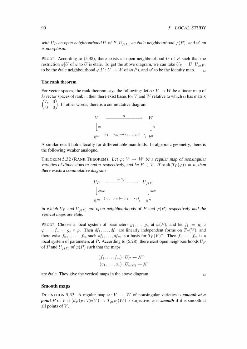
90 5 LOCAL STUDY

with UP an open neighbourhood U of P , Uf(P ) an etale neighbourhood ϕ(P ), and ϕ′ anisomorphism.

PROOF. According to (5.38), there exists an open neighbourhood U of P such that therestriction ϕ|U of ϕ to U is etale. To get the above diagram, we can take UP = U , Uϕ(P )

to be the etale neighbourhood ϕ|U : U →W of ϕ(P ), and ϕ′ to be the identity map. 2

The rank theorem

For vector spaces, the rank theorem says the following: let α : V → W be a linear map ofk-vector spaces of rank r; then there exist bases for V andW relative to which α has matrix(Ir 00 0

). In other words, there is a commutative diagram

Vα−−−−−−−−−−−−−→ Wy≈ y≈

km(x1,...,xm) 7→(x1,...,xr,0,...)−−−−−−−−−−−−−−−−→ kn

A similar result holds locally for differentiable manifolds. In algebraic geometry, there isthe following weaker analogue.

THEOREM 5.32 (RANK THEOREM). Let ϕ : V → W be a regular map of nonsingularvarieties of dimensions m and n respectively, and let P ∈ V . If rank(TP (ϕ)) = n, thenthere exists a commutative diagram

UPϕ|UP−−−−−−−−−−−−→ Uϕ(P )yetale

yetale

Am (x1,...,xm) 7→(x1,...,xn)−−−−−−−−−−−−−−→ An

in which UP and Uϕ(P ) are open neighbourhoods of P and ϕ(P ) respectively and thevertical maps are etale.

PROOF. Choose a local system of parameters g1, . . . , gn at ϕ(P ), and let f1 = g1 ϕ, . . . , fn = gn ϕ. Then df1, . . . , dfn are linearly independent forms on TP (V ), andthere exist fn+1, . . . , fm such df1, . . . , dfm is a basis for TP (V )∨. Then f1, . . . , fm is alocal system of parameters at P . According to (5.28), there exist open neighbourhoods UPof P and Uϕ(P ) of ϕ(P ) such that the maps

(f1, . . . , fm) : UP → Am

(g1, . . . , gn) : Uϕ(P ) → An

are etale. They give the vertical maps in the above diagram. 2

Smooth maps

DEFINITION 5.33. A regular map ϕ : V → W of nonsingular varieties is smooth at apoint P of V if (dϕ)P : TP (V ) → Tϕ(P )(W ) is surjective; ϕ is smooth if it is smooth atall points of V .

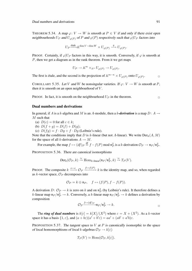
Dual numbers and derivations 91

THEOREM 5.34. A map ϕ : V → W is smooth at P ∈ V if and only if there exist openneighbourhoods UP and Uϕ(P ) of P and ϕ(P ) respectively such that ϕ|UP factors into

UPetale−−→AdimV−dimW × Uϕ(P )

q−→ Uϕ(P ).

PROOF. Certainly, if ϕ|UP factors in this way, it is smooth. Conversely, if ϕ is smooth atP , then we get a diagram as in the rank theorem. From it we get maps

UP → Am ×An Uϕ(P ) → Uϕ(P ).

The first is etale, and the second is the projection of Am−n × Uϕ(P ) onto Uϕ(P ). 2

COROLLARY 5.35. Let V and W be nonsingular varieties. If ϕ : V → W is smooth at P ,then it is smooth on an open neighbourhood of V .

PROOF. In fact, it is smooth on the neighbourhood UP in the theorem. 2

Dual numbers and derivations

In general, ifA is a k-algebra andM is anA-module, then a k-derivation is a mapD : A→M such that

(a) D(c) = 0 for all c ∈ k;(b) D(f + g) = D(f) +D(g);(c) D(fg) = f ·Dg + f ·Dg (Leibniz’s rule).

Note that the conditions imply that D is k-linear (but not A-linear). We write Derk(A,M)for the space of all k-derivations A→M .

For example, the map f 7→ (df)Pdf= f−f(P ) mod n2

P is a k-derivationOP → nP /n2P .

PROPOSITION 5.36. There are canonical isomorphisms

Derk(OP , k)'→ Homk-linear(nP /n2

P , k)'→ TP (V ).

PROOF. The composite k c 7→c−−→ OPf 7→f(P )−−−−−→ k is the identity map, and so, when regarded

as k-vector space, OP decomposes into

OP = k ⊕ nP , f ↔ (f(P ), f − f(P )).

A derivation D : OP → k is zero on k and on n2P (by Leibniz’s rule). It therefore defines a

k-linear map nP /n2P → k. Conversely, a k-linear map nP /n

2P → k defines a derivation by

composition

OPf 7→(df)P−−−−−→nP /n

2P → k. 2

The ring of dual numbers is k[ε] = k[X]/(X2) where ε = X + (X2). As a k-vectorspace it has a basis 1, ε, and (a+ bε)(a′ + b′ε) = aa′ + (ab′ + a′b)ε.

PROPOSITION 5.37. The tangent space to V at P is canonically isomorphic to the spaceof local homomorphisms of local k-algebras OP → k[ε]:

TP (V ) ' Hom(OP , k[ε]).

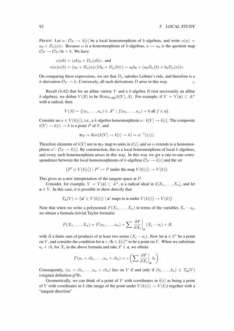
92 5 LOCAL STUDY

PROOF. Let α : OP → k[ε] be a local homomorphism of k-algebras, and write α(a) =a0 + Dα(a)ε. Because α is a homomorphism of k-algebras, a 7→ a0 is the quotient mapOP → OP /m = k. We have

α(ab) = (ab)0 +Dα(ab)ε, and

α(a)α(b) = (a0 +Dα(a)ε)(b0 +Dα(b)ε) = a0b0 + (a0Dα(b) + b0Dα(a))ε.

On comparing these expressions, we see that Dα satisfies Leibniz’s rule, and therefore is ak-derivation OP → k. Conversely, all such derivations D arise in this way. 2

Recall (4.42) that for an affine variety V and a k-algebra R (not necessarily an affinek-algebra), we define V (R) to be Homk-alg(k[V ], A). For example, if V = V (a) ⊂ An

with a radical, then

V (A) = (a1, . . . , an) ∈ An | f(a1, . . . , an) = 0 all f ∈ a.

Consider an α ∈ V (k[ε]), i.e., a k-algebra homomorphism α : k[V ]→ k[ε]. The compositek[V ]→ k[ε]→ k is a point P of V , and

mP = Ker(k[V ]→ k[ε]→ k) = α−1((ε)).

Therefore elements of k[V ] not in mP map to units in k[ε], and so α extends to a homomor-phism α′ : OP → k[ε]. By construction, this is a local homomorphism of local k-algebras,and every such homomorphism arises in this way. In this way we get a one-to-one corre-spondence between the local homomorphisms of k-algebras OP → k[ε] and the set

P ′ ∈ V (k[ε]) | P ′ 7→ P under the map V (k[ε])→ V (k).

This gives us a new interpretation of the tangent space at P .Consider, for example, V = V (a) ⊂ An, a a radical ideal in k[X1, . . . , Xn], and let

a ∈ V . In this case, it is possible to show directly that

Ta(V ) = a′ ∈ V (k[ε]) | a′ maps to a under V (k[ε])→ V (k)

Note that when we write a polynomial F (X1, . . . , Xn) in terms of the variables Xi − ai,we obtain a formula (trivial Taylor formula)

F (X1, . . . , Xn) = F (a1, . . . , an) +∑ ∂F

∂Xi

∣∣∣∣a

(Xi − ai) +R

with R a finite sum of products of at least two terms (Xi − ai). Now let a ∈ kn be a pointon V , and consider the condition for a+εb ∈ k[ε]n to be a point on V . When we substituteai + εbi for Xi in the above formula and take F ∈ a, we obtain:

F (a1 + εb1, . . . , an + εbn) = ε

(∑ ∂F

∂Xi

∣∣∣∣a

bi

).

Consequently, (a1 + εb1, . . . , an + εbn) lies on V if and only if (b1, . . . , bn) ∈ Ta(V )(original definition p78).

Geometrically, we can think of a point of V with coordinates in k[ε] as being a pointof V with coordinates in k (the image of the point under V (k[ε])→ V (k)) together with a“tangent direction”

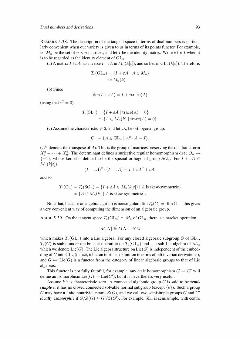
Dual numbers and derivations 93

REMARK 5.38. The description of the tangent space in terms of dual numbers is particu-larly convenient when our variety is given to us in terms of its points functor. For example,let Mn be the set of n × n matrices, and let I be the identity matrix. Write e for I when itis to be regarded as the identity element of GLn.

(a) A matrix I+εA has inverse I−εA inMn(k[ε]), and so lies in GLn(k[ε]). Therefore,

Te(GLn) = I + εA | A ∈Mn'Mn(k).

(b) Sincedet(I + εA) = I + εtrace(A)

(using that ε2 = 0),

Te(SLn) = I + εA | trace(A) = 0' A ∈Mn(k) | trace(A) = 0.

(c) Assume the characteristic 6= 2, and let On be orthogonal group:

On = A ∈ GLn | Atr ·A = I.

(Atr denotes the transpose ofA). This is the group of matrices preserving the quadratic formX2

1 + · · · +X2n. The determinant defines a surjective regular homomorphism det : On →

±1, whose kernel is defined to be the special orthogonal group SOn. For I + εA ∈Mn(k[ε]),

(I + εA)tr · (I + εA) = I + εAtr + εA,

and so

Te(On) = Te(SOn) = I + εA ∈Mn(k[ε]) | A is skew-symmetric' A ∈Mn(k) | A is skew-symmetric.

Note that, because an algebraic group is nonsingular, dimTe(G) = dimG — this givesa very convenient way of computing the dimension of an algebraic group.

ASIDE 5.39. On the tangent space Te(GLn) 'Mn of GLn, there is a bracket operation

[M,N ] df= MN −NM

which makes Te(GLn) into a Lie algebra. For any closed algebraic subgroup G of GLn,Te(G) is stable under the bracket operation on Te(GLn) and is a sub-Lie-algebra of Mn,which we denote Lie(G). The Lie algebra structure on Lie(G) is independent of the embed-ding ofG into GLn (in fact, it has an intrinsic definition in terms of left invarian derivations),and G 7→ Lie(G) is a functor from the category of linear algebraic groups to that of Liealgebras.

This functor is not fully faithful, for example, any etale homomorphism G → G′ willdefine an isomorphism Lie(G)→ Lie(G′), but it is nevertheless very useful.

Assume k has characteristic zero. A connected algebraic group G is said to be semi-simple if it has no closed connected solvable normal subgroup (except e). Such a groupG may have a finite nontrivial centre Z(G), and we call two semisimple groups G and G′

locally isomorphic if G/Z(G) ≈ G′/Z(G′). For example, SLn is semisimple, with centre

94 5 LOCAL STUDY

µn, the set of diagonal matrices diag(ζ, . . . , ζ), ζn = 1, and SLn /µn = PSLn. A Liealgebra is semisimple if it has no commutative ideal (except 0). One can prove that

G is semisimple ⇐⇒ Lie(G) is semisimple,

and the map G 7→ Lie(G) defines a one-to-one correspondence between the set of localisomorphism classes of semisimple algebraic groups and the set of isomorphism classes ofLie algebras. The classification of semisimple algebraic groups can be deduced from that ofsemisimple Lie algebras and a study of the finite coverings of semisimple algebraic groups— this is quite similar to the relation between Lie groups and Lie algebras.

Tangent cones

In this subsection, I assume familiarity with parts of Atiyah and MacDonald 1969, Chapters11, 12.

Let V = V (a) ⊂ km, a = rad(a), and let P = (0, . . . , 0) ∈ V . Define a∗ to be theideal generated by the polynomials F∗ for F ∈ a, where F∗ is the leading form of F (seep77). The geometric tangent cone at P , CP (V ) is V (a∗), and the tangent cone is the pair(V (a∗), k[X1, . . . , Xn]/a∗). Obviously, CP (V ) ⊂ TP (V ).

Computing the tangent cone

If a is principal, say a = (F ), then a∗ = (F∗), but if a = (F1, . . . , Fr), then it need notbe true that a∗ = (F1∗, . . . , Fr∗). Consider for example a = (XY,XZ + Z(Y 2 − Z2)).One can show that this is a radical ideal either by asking Macaulay (assuming you believeMacaulay), or by following the method suggested in Cox et al. 1992, p474, problem 3 toshow that it is an intersection of prime ideals. Since

Y Z(Y 2 − Z2) = Y · (XZ + Z(Y 2 − Z2))− Z · (XY ) ∈ a

and is homogeneous, it is in a∗, but it is not in the ideal generated by XY , XZ. In fact, a∗is the ideal generated by

XY, XZ, Y Z(Y 2 − Z2).

This raises the following question: given a set of generators for an ideal a, how do youfind a set of generators for a∗? There is an algorithm for this in Cox et al. 1992, p467. Leta be an ideal (not necessarily radical) such that V = V (a), and assume the origin is in V .Introduce an extra variable T such that T “>” the remaining variables. Make each generatorof a homogeneous by multiplying its monomials by appropriate (small) powers of T , andfind a Grobner basis for the ideal generated by these homogeneous polynomials. RemoveT from the elements of the basis, and then the polynomials you get generate a∗.

Intrinsic definition of the tangent cone

Let A be a local ring with maximal ideal n. The associated graded ring is

gr(A) =⊕

i≥0ni/ni+1.

Note that if A = Bm and n = mA, then gr(A) =⊕

mi/mi+1 (because of (1.31)).

Exercises 95

PROPOSITION 5.40. The map k[X1, . . . , Xn]/a∗ → gr(OP ) sending the class of Xi ink[X1, . . . , Xn]/a∗ to the class of Xi in gr(OP ) is an isomorphism.

PROOF. Let m be the maximal ideal in k[X1, . . . , Xn]/a corresponding to P . Then

gr(OP ) =∑

mi/mi+1

=∑

(X1, . . . , Xn)i/(X1, . . . , Xn)i+1 + a ∩ (X1, . . . , Xn)i

=∑

(X1, . . . , Xn)i/(X1, . . . , Xn)i+1 + ai

where ai is the homogeneous piece of a∗ of degree i (that is, the subspace of a∗ consistingof homogeneous polynomials of degree i). But

(X1, . . . , Xn)i/(X1, . . . , Xn)i+1 + ai = ith homogeneous piece of k[X1, . . . , Xn]/a∗.

2

For a general variety V and P ∈ V , we define the geometric tangent cone CP (V ) ofV at P to be Spm(gr(OP )red), where gr(OP )red is the quotient of gr(OP ) by its nilradical,and we define the tangent cone to be (CP (V ), gr(OP )).

Recall (Atiyah and MacDonald 1969, 11.21) that dim(A) = dim(gr(A)). Thereforethe dimension of the geometric tangent cone at P is the same as the dimension of V (incontrast to the dimension of the tangent space).

Recall (ibid., 11.22) that gr(OP ) is a polynomial ring in d variables (d = dimV ) if andonly if OP is regular. Therefore, P is nonsingular if and only if gr(OP ) is a polynomialring in d variables, in which case CP (V ) = TP (V ).

Using tangent cones, we can extend the notion of an etale morphism to singular va-rieties. Obviously, a regular map α : V → W induces a homomorphism gr(Oα(P )) →gr(OP ). We say that α is etale at P if this is an isomorphism. Note that then there is anisomorphism of the geometric tangent cones CP (V )→ Cα(P )(W ), but this map may be anisomorphism without α being etale at P . Roughly speaking, to be etale at P , we need themap on geometric tangent cones to be an isomorphism and to preserve the “multiplicities”of the components.

It is a fairly elementary result that a local homomorphism of local rings α : A → Binduces an isomorphism on the graded rings if and only if it induces an isomorphism on thecompletions (ibid., 10.23). Thus α : V → W is etale at P if and only if the map Oα(P ) →OP is an isomorphism. Hence (5.27) shows that the choice of a local system of parametersf1, . . . , fd at a nonsingular point P determines an isomorphism OP → k[[X1, . . . , Xd]].

We can rewrite this as follows: let t1, . . . , td be a local system of parameters at a non-singular point P ; then there is a canonical isomorphism OP → k[[t1, . . . , td]]. For f ∈ OP ,the image of f ∈ k[[t1, . . . , td]] can be regarded as the Taylor series of f .

For example, let V = A1, and let P be the point a. Then t = X−a is a local parameterat a, OP consists of quotients f(X) = g(X)/h(X) with h(a) 6= 0, and the coefficientsof the Taylor expansion

∑n≥0 an(X − a)n of f(X) can be computed as in elementary

calculus courses: an = f (n)(a)/n!.

Exercises

5-1. Find the singular points, and the tangent cones at the singular points, for each of

96 5 LOCAL STUDY

(a) Y 3 − Y 2 +X3 −X2 + 3Y 2X + 3X2Y + 2XY ;(b) X4 + Y 4 −X2Y 2 (assume the characteristic is not 2).

5-2. Let V ⊂ An be an irreducible affine variety, and let P be a nonsingular point on V .Let H be a hyperplane in An (i.e., the subvariety defined by a linear equation

∑aiXi = d

with not all ai zero) passing through P but not containing TP (V ). Show that P is a nonsin-gular point on each irreducible component of V ∩ H on which it lies. (Each irreduciblecomponent has codimension 1 in V — you may assume this.) Give an example withH ⊃ TP (V ) and P singular on V ∩H . Must P be singular on V ∩H if H ⊃ TP (V )?

5-3. Let P and Q be points on varieties V and W . Show that

T(P,Q)(V ×W ) = TP (V )⊕ TQ(W ).

5-4. For each n, show that there is a curve C and a point P on C such that the tangentspace to C at P has dimension n (hence C can’t be embedded in An−1 ).

5-5. Let I be the n×n identity matrix, and let J be the matrix(

0 I−I 0

). The symplectic

group Spn is the group of 2n×2n matrices A with determinant 1 such that Atr ·J ·A = J .(It is the group of matrices fixing a nondegenerate skew-symmetric form.) Find the tangentspace to Spn at its identity element, and also the dimension of Spn.

5-6. Find a regular map α : V → W which induces an isomorphism on the geometrictangent cones CP (V )→ Cα(P )(W ) but is not etale at P .

5-7. Show that the cone X2 + Y 2 = Z2 is a normal variety, even though the origin issingular (characteristic 6= 2). See p88.

5-8. Let V = V (a) ⊂ An. Suppose that a 6= I(V ), and for a ∈ V , let T ′a be the subspaceof Ta(An) defined by the equations (df)a = 0, f ∈ a. Clearly, T ′a ⊃ Ta(V ), but need theyalways be different?

97

6 Projective Varieties

Throughout this section, k will be an algebraically closed field. Recall (4.3) that we definedPn to be the set of equivalence classes in kn+1 r origin for the relation

(a0, . . . , an) ∼ (b0, . . . , bn) ⇐⇒ (a0, . . . , an) = c(b0, . . . , bn) for some c ∈ k×.

Write (a0 : . . . : an) for the equivalence class of (a0, . . . , an), and π for the map

kn+1 r origin/∼→ Pn.

Let Ui be the set of (a0 : . . . : an) ∈ Pn such that ai 6= 0, and let ui be the bijection

(a0 : . . . : an) 7→(a0ai, . . . , an

ai

): Ui 7→ An (ai

aiomitted).

In this section, we shall define on Pn a (unique) structure of an algebraic variety for whichthese maps become isomorphisms of affine algebraic varieties. A variety isomorphic to aclosed subvariety of Pn is called a projective variety, and a variety isomorphic to a locallyclosed subvariety of Pn is called a quasi-projective variety.35 Every affine variety is qua-siprojective, but there are many varieties that are not quasiprojective. We study morphismsbetween quasiprojective varieties.

Projective varieties are important for the same reason compact manifolds are important:results are often simpler when stated for projective varieties, and the “part at infinity” oftenplays a role, even when we would like to ignore it. For example, a famous theorem ofBezout (see 6.34 below) says that a curve of degree m in the projective plane intersects acurve of degree n in exactly mn points (counting multiplicities). For affine curves, one hasonly an inequality.

Algebraic subsets of Pn

A polynomial F (X0, . . . , Xn) is said to be homogeneous of degree d if it is a sum of termsai0,...,inX

i00 · · ·Xin

n with i0 + · · ·+ in = d; equivalently,

F (tX0, . . . , tXn) = tdF (X0, . . . , Xn)

for all t ∈ k. Write k[X0, . . . , Xn]d for the subspace of k[X0, . . . , Xn] of polynomials ofdegree d. Then

k[X0, . . . , Xn] =⊕d≥0

k[X0, . . . , Xn]d;

that is, each polynomial F can be written uniquely as a sum F =∑Fd with Fd homoge-

neous of degree d.Let P = (a0 : . . . : an) ∈ Pn. Then P also equals (ca0 : . . . : can) for any c ∈ k×,

and so we can’t speak of the value of a polynomial F (X0, . . . , Xn) at P . However, if F ishomogeneous, then F (ca0, . . . , can) = cdF (a0, . . . , an), and so it does make sense to saythat F is zero or not zero at P . An algebraic set in Pn (or projective algebraic set) is theset of common zeros in Pn of some set of homogeneous polynomials.

35A subvariety of an affine variety is said to be quasi-affine. For example, A2 r (0, 0) is quasi-affine butnot affine.

98 6 PROJECTIVE VARIETIES

EXAMPLE 6.1. Consider the projective algebraic subset E of P2 defined by the homoge-neous equation

Y 2Z = X3 + aXZ2 + bZ3 (12)

whereX3+aX+b is assumed not to have multiple roots. It consists of the points (x : y : 1)on the affine curve E ∩ U2

Y 2 = X3 + aX + b,

together with the point “at infinity” (0 : 1 : 0).Curves defined by equations of the form (12) are called elliptic curves. They can also

be described as the curves of genus one, or as the abelian varieties of dimension one. Sucha curve becomes an algebraic group, with the group law such that P + Q + R = 0 if andonly if P , Q, and R lie on a straight line. The zero for the group is the point at infinity.(Without the point at infinity, it is not possible to make E into an algebraic group.)

When a, b ∈ Q, we can speak of the zeros of (*) with coordinates in Q. They also forma group E(Q), which Mordell showed to be finitely generated. It is easy to compute thetorsion subgroup of E(Q), but there is at present no known algorithm for computing therank of E(Q). More precisely, there is an “algorithm” which always works, but which hasnot been proved to terminate after a finite amount of time, at least not in general. There isa very beautiful theory surrounding elliptic curves over Q and other number fields, whoseorigins can be traced back 1,800 years to Diophantus. (See my notes on Elliptic Curves forall of this.)

An ideal a ⊂ k[X0, . . . , Xn] is said to be homogeneous if it contains with any polyno-mial F all the homogeneous components of F , i.e., if

F ∈ a =⇒ Fd ∈ a, all d.

It is straightforward to check that— an ideal is homogeneous if and only if it is generated by (a finite set of) homogeneous

polynomials;— the radical of a homogeneous ideal is homogeneous;— an intersection, product, or sum of homogeneous ideals is homogeneous.

For a homogeneous ideal a, we write V (a) for the set of common zeros of the homoge-neous polynomials in a. If F1, . . . , Fr are homogeneous generators for a, then V (a) is theset of common zeros of the Fi. Clearly every polynomial in a is zero on every representativeof a point in V (a). We write V aff(a) for the set of common zeros of a in kn+1. It is cone inkn+1, i.e., together with any point P it contains the line through P and the origin, and

V (a) = (V aff(a) r (0, . . . , 0))/∼ .

The sets V (a) have similar properties to their namesakes in An.

PROPOSITION 6.2. There are the following relations:(a) a ⊂ b⇒ V (a) ⊃ V (b);(b) V (0) = Pn; V (a) = ∅ ⇐⇒ rad(a) ⊃ (X0, . . . , Xn);(c) V (ab) = V (a ∩ b) = V (a) ∪ V (b);(d) V (

∑ai) =

⋂V (ai).

Algebraic subsets of Pn 99

PROOF. Statement (a) is obvious. For the second part of (b), note that

V (a) = ∅ ⇐⇒ V aff(a) ⊂ (0, . . . , 0) ⇐⇒ rad(a) ⊃ (X0, . . . , Xn),

by the strong Nullstellensatz (2.11). The remaining statements can be proved directly, orby using the relation between V (a) and V aff(a). 2

IfC is a cone in kn+1, then I(C) is a homogeneous ideal in k[X0, . . . , Xn]: ifF (ca0, . . . , can) =0 for all c ∈ k×, then∑

d

Fd(a0, . . . , an) · cd = F (ca0, . . . , can) = 0,

for infinitely many c, and so∑Fd(a0, . . . , an)Xd is the zero polynomial. For a subset S

of Pn, we define the affine cone over S in kn+1 to be

C = π−1(S) ∪ origin

and we setI(S) = I(C).

Note that if S is nonempty and closed, then C is the closure of π−1(S) = ∅, and that I(S)is spanned by the homogeneous polynomials in k[X0, . . . , Xn] that are zero on S.

PROPOSITION 6.3. The maps V and I define inverse bijections between the set of alge-braic subsets of Pn and the set of proper homogeneous radical ideals of k[X0, . . . , Xn].An algebraic set V in Pn is irreducible if and only if I(V ) is prime; in particular, Pn isirreducible.

PROOF. Note that we have bijections

algebraic subsets of Pn S 7→C> nonempty closed cones in kn+1

proper homogeneous radical ideals in k[X0, . . . , Xn]

I

<

V

<

Here the top map sends S to the affine cone over S, and the maps V and I are in the sense ofprojective geometry and affine geometry respectively. The composite of any three of thesemaps is the identity map, which proves the first statement because the composite of the topmap with I is I in the sense of projective geometry. Obviously, V is irreducible if and onlyif the closure of π−1(V ) is irreducible, which is true if and only if I(V ) is a prime ideal. 2

Note that (X0, . . . , Xn) and k[X0, . . . , Xn] are both radical homogeneous ideals, but

V (X0, . . . , Xn) = ∅ = V (k[X0, . . . , Xn])

and so the correspondence between irreducible subsets of Pn and radical homogeneousideals is not quite one-to-one.

100 6 PROJECTIVE VARIETIES

The Zariski topology on Pn

Proposition 6.2 shows that the projective algebraic sets are the closed sets for a topology onPn. In this subsection, we verify that it agrees with that defined in the first paragraph of thissection. For a homogeneous polynomial F , let

D(F ) = P ∈ Pn | F (P ) 6= 0.

Then, just as in the affine case, D(F ) is open and the sets of this type form a base for thetopology of Pn.

To each polynomial f(X1, . . . , Xn), we attach the homogeneous polynomial of thesame degree

f∗(X0, . . . , Xn) = Xdeg(f)0 f

(X1X0, . . . , Xn

X0

),

and to each homogeneous polynomial F (X0, . . . , Xn), we attach the polynomial

F∗(X1, . . . , Xn) = F (1, X1, . . . , Xn).

PROPOSITION 6.4. For the topology on Pn just defined, each Ui is open, and when weendow it with the induced topology, the bijection

Ui ↔ An, (a0 : . . . : 1 : . . . : an)↔ (a0, . . . , ai−1, ai+1, . . . , an)

becomes a homeomorphism.

PROOF. It suffices to prove this with i = 0. The set U0 = D(X0), and so it is a basic opensubset in Pn. Clearly, for any homogeneous polynomial F ∈ k[X0, . . . , Xn],

D(F (X0, . . . , Xn)) ∩ U0 = D(F (1, X1, . . . , Xn)) = D(F∗)

and, for any polynomial f ∈ k[X1, . . . , Xn],

D(f) = D(f∗) ∩ U0.

Thus, under U0 ↔ An, the basic open subsets of An correspond to the intersections withUi of the basic open subsets of Pn, which proves that the bijection is a homeomorphism. 2

REMARK 6.5. It is possible to use this to give a different proof that Pn is irreducible. Weapply the criterion that a space is irreducible if and only if every nonempty open subset isdense (see p37). Note that each Ui is irreducible, and that Ui∩Uj is open and dense in eachof Ui and Uj (as a subset of Ui, it is the set of points (a0 : . . . : 1 : . . . : aj : . . . : an) withaj 6= 0). Let U be a nonempty open subset of Pn; then U ∩ Ui is open in Ui. For somei, U ∩ Ui is nonempty, and so must meet Ui ∩ Uj . Therefore U meets every Uj , and so isdense in every Uj . It follows that its closure is all of Pn.

Closed subsets of An and Pn

We identify An with U0, and examine the closures in Pn of closed subsets of An. Note that

Pn = An tH∞, H∞ = V (X0).

With each ideal a in k[X1, . . . , Xn], we associate the homogeneous ideal a∗ in k[X0, . . . , Xn]generated by f∗ | f ∈ a. For a closed subset V of An, set V ∗ = V (a∗) with a = I(V ).

With each homogeneous ideal a in k[X0, X1, . . . , Xn], we associate the ideal a∗ ink[X1, . . . , Xn] generated by F∗ | F ∈ a. When V is a closed subset of Pn, we setV∗ = V (a∗) with a = I(V ).

The hyperplane at infinity 101

PROPOSITION 6.6. (a) Let V be a closed subset of An. Then V ∗ is the closure of V in Pn,and (V ∗)∗ = V . If V =

⋃Vi is the decomposition of V into its irreducible components,

then V ∗ =⋃V ∗i is the decomposition of V ∗ into its irreducible components.

(b) Let V be a closed subset of Pn. Then V∗ = V ∩An, and if no irreducible componentof V lies in H∞ or contains H∞, then V∗ is a proper subset of An, and (V∗)∗ = V .

PROOF. Straightforward. 2

EXAMPLE 6.7. (a) ForV : Y 2 = X3 + aX + b,

we haveV ∗ : Y 2Z = X3 + aXZ2 + bZ3,

and (V ∗)∗ = V .(b) Let V = V (f1, . . . , fm); then the closure of V in Pn is the union of the irreducible

components of V (f∗1 , . . . , f∗m) not contained in H∞. For example, let V = V (X1, X

21 +

X2) = (0, 0); then V (X0X1, X21 + X0X2) consists of the two points (1 : 0 : 0) (the

closure of V ) and (0 : 0 : 1) (which is contained in H∞).36

(b) For V = H∞ = V (X0), V∗ = ∅ = V (1) and (V∗)∗ = ∅ 6= V .

The hyperplane at infinity

It is often convenient to think of Pn as being An = U0 with a hyperplane added “at infinity”.More precisely, identify the U0 with An. The complement of U0 in Pn is

H∞ = (0 : a1 : . . . : an) ⊂ Pn,

which can be identified with Pn−1.For example, P1 = A1 t H∞ (disjoint union), with H∞ consisting of a single point,

and P2 = A2 ∪H∞ with H∞ a projective line. Consider the line

1 + aX1 + bX2 = 0

in A2. Its closure in P2 is the line

X0 + aX1 + bX2 = 0.

This line intersects the line H∞ = V (X0) at the point (0 : −b : a), which equals (0 : 1 :−a/b) when b 6= 0. Note that −a/b is the slope of the line 1 + aX1 + bX2 = 0, and sothe point at which a line intersects H∞ depends only on the slope of the line: parallel linesmeet in one point at infinity. We can think of the projective plane P2 as being the affineplane A2 with one point added at infinity for each direction in A2.

Similarly, we can think of Pn as being An with one point added at infinity for eachdirection in An — being parallel is an equivalence relation on the lines in An, and there isone point at infinity for each equivalence class of lines.

We can also identify An with Un, as in Example 6.1. Note that in this case the point atinfinity on the elliptic curve Y 2 = X3 + aX + b is the intersection of the closure of anyvertical line with H∞.

36Of course, in this case a = (X1, X2), a∗ = (X1, X2), and V ∗ = (1 : 0 : 0), and so this exampledoesn’t contradict the proposition.

102 6 PROJECTIVE VARIETIES

Pn is an algebraic variety

For each i, writeOi for the sheaf onUi ⊂ Pn defined by the homeomorphism ui : Ui → An.

LEMMA 6.8. Write Uij = Ui ∩Uj ; then Oi|Uij = Oj |Uij . When endowed with this sheafUij is an affine variety; moreover, Γ (Uij ,Oi) is generated as a k-algebra by the functions(f |Uij)(g|Uij) with f ∈ Γ (Ui,Oi), g ∈ Γ (Uj ,Oj).

PROOF. It suffices to prove this for (i, j) = (0, 1). All rings occurring in the proof will beidentified with subrings of the field k(X0, X1, . . . , Xn).

Recall that

U0 = (a0 : a1 : . . . : an) | a0 6= 0; (a0 : a1 : . . . : an)↔ (a1a0, a2a0, . . . , an

a0) ∈ An.

Let k[X1X0, X2X0, . . . , Xn

X0] be the subring of k(X0, X1, . . . , Xn) generated by the quotients Xi

X0

— it is the polynomial ring in the n symbols X1X0, . . . , Xn

X0. An element f(X1

X0, . . . , Xn

X0) ∈

k[X1X0, . . . , Xn

X0] defines a map

(a0 : a1 : . . . : an) 7→ f(a1a0, . . . , an

a0) : U0 → k,

and in this way k[X1X0, X2X0, . . . , Xn

X0] becomes identified with the ring of regular functions on

U0, and U0 with Spm(k[X1X0, . . . , Xn

X0])

.Next consider the open subset of U0,

U01 = (a0 : . . . : an) | a0 6= 0, a1 6= 0.

It is D(X1X0

), and is therefore an affine subvariety of (U0,O0). The inclusion U01 →U0 corresponds to the inclusion of rings k[X1

X0, . . . , Xn

X0] → k[X1

X0, . . . , Xn

X0, X0X1

]. An ele-ment f(X1

X0, . . . , Xn

X0, X0X1

) of k[X1X0, . . . , Xn

X0, X0X1

] defines the function (a0 : . . . : an) 7→f(a1

a0, . . . , an

a0, a0a1

) on U01.Similarly,

U1 = (a0 : a1 : . . . : an) | a1 6= 0; (a0 : a1 : . . . : an)↔ (a0a1, . . . , an

a1) ∈ An,

and we identify U1 with Spm(k[X0X1, X2X0, . . . , Xn

X1])

. A polynomial f(X0X1, . . . , Xn

X1) in

k[X0X1, . . . , Xn

X1] defines the map (a0 : . . . : an) 7→ f(a0

a1, . . . , an

a1) : U1 → k.

When regarded as an open subset of U1, U01 = D(X0X1

), and is therefore an affinesubvariety of (U1,O1), and the inclusion U01 → U1 corresponds to the inclusion of ringsk[X0X1, . . . , Xn

X1] → k[X0

X1, . . . , Xn

X1, X1X0

]. An element f(X0X1, . . . , Xn

X1, X1X0

) of k[X0X1, . . . , Xn

X1, X1X0

]defines the function (a0 : . . . : an) 7→ f(a0

a1, . . . , an

a1, a1a0

) on U01.The two subrings k[X1

X0, . . . , Xn

X0, X0X1

] and k[X0X1, . . . , Xn

X1, X1X0

] of k(X0, X1, . . . , Xn) areequal, and an element of this ring defines the same function on U01 regardless of which ofthe two rings it is considered an element. Therefore, whether we regard U01 as a subvarietyof U0 or of U1 it inherits the same structure as an affine algebraic variety (3.8a). Thisproves the first two assertions, and the third is obvious: k[X1

X0, . . . , Xn

X0, X0X1

] is generated byits subrings k[X1

X0, . . . , Xn

X0] and k[X0

X1, X2X1, . . . , Xn

X1]. 2

PROPOSITION 6.9. There is a unique structure of a (separated) algebraic variety on Pn forwhich each Ui is an open affine subvariety of Pn and each map ui is an isomorphism ofalgebraic varieties.

The homogeneous coordinate ring of a subvariety of Pn 103

PROOF. Endow each Ui with the structure of an affine algebraic variety for which ui isan isomorphism. Then Pn =

⋃Ui, and the lemma shows that this covering satisfies the

patching condition (4.13), and so Pn has a unique structure of a ringed space for whichUi → Pn is a homeomorphism onto an open subset of Pn and OPn |Ui = OUi . Moreover,because each Ui is an algebraic variety, this structure makes Pn into an algebraic prevariety.Finally, the lemma shows that Pn satisfies the condition (4.27c) to be separated. 2

EXAMPLE 6.10. Let C be the plane projective curve

C : Y 2Z = X3

and assume char(k) 6= 2. For each a ∈ k×, there is an automorphism

(x : y : z) 7→ (ax : y : a3z) : Cϕa−→ C.

Patch two copies of C × A1 together along C × (A1 − 0) by identifying (P, u) with(ϕa(P ), a−1), P ∈ C, a ∈ A1 r 0. One obtains in this way a singular 2-dimensionalvariety that is not quasiprojective (see Hartshorne 1977, Exercise 7.13). It is even complete— see below — and so if it were quasiprojective, it would be projective. It is knownthat every irreducible separated curve is quasiprojective, and every nonsingular completesurface is projective, and so this is an example of minimum dimension. In Shafarevich1994, VI 2.3, there is an example of a nonsingular complete variety of dimension 3 that isnot projective.

The homogeneous coordinate ring of a subvariety of Pn

Recall (page 40) that we attached to each irreducible variety V a field k(V ) with the prop-erty that k(V ) is the field of fractions of k[U ] for any open affine U ⊂ V . We now describethis field in the case that V = Pn. Recall that k[U0] = k[X1

X0, . . . , Xn

X0]. We regard this as a

subring of k(X0, . . . , Xn), and wish to identify the field of fractions of k[U0] as a subfieldof k(X0, . . . , Xn). Any nonzero F ∈ k[U0] can be written

F (X1X0, . . . , Xn

X0) =

F ∗(X0, . . . , Xn)

Xdeg(F )0

with F ∗ homogeneous of degree deg(F ), and it follows that the field of fractions of k[U0]is

k(U0) =G(X0, . . . , Xn)H(X0, . . . , Xn)

∣∣∣∣ G, H homogeneous of the same degree∪ 0.

Write k(X0, . . . , Xn)0 for this field (the subscript 0 is short for “subfield of elements ofdegree 0”), so that k(Pn) = k(X0, . . . , Xn)0. Note that for F = G

H in k(X0, . . . , Xn)0,

(a0 : . . . : an) 7→G(a0, . . . , an)H(a0, . . . , an)

: D(H)→ k,

is a well-defined function, which is obviously regular (look at its restriction to Ui).We now extend this discussion to any irreducible projective variety V . Such a V can be

written V = V (p) with p a homogeneous radical ideal in k[X0, . . . , Xn], and we define thehomogeneous coordinate ring of V (with its given embedding) to be

khom[V ] = k[X0, . . . , Xn]/p.

104 6 PROJECTIVE VARIETIES

Note that khom[V ] is the ring of regular functions on the affine cone over V ; therefore itsdimension is dim(V ) + 1. It depends, not only on V , but on the embedding of V intoPn, i.e., it is not intrinsic to V (see 6.19 below). We say that a nonzero f ∈ khom[V ]is homogeneous of degree d if it can be represented by a homogeneous polynomial F ofdegree d in k[X0, . . . , Xn] (we say that 0 is homogeneous of degree 0).

LEMMA 6.11. Each element of khom[V ] can be written uniquely in the form

f = f0 + · · ·+ fd

with fi homogeneous of degree i.

PROOF. Let F represent f ; then F can be written F = F0 + · · ·+Fd with Fi homogeneousof degree i, and when reduced modulo p, this gives a decomposition of f of the requiredtype. Suppose f also has a decomposition f =

∑gi, with gi represented by the homoge-

neous polynomial Gi of degree i. Then F −G ∈ p, and the homogeneity of p implies thatFi −Gi = (F −G)i ∈ p. Therefore fi = gi. 2

It therefore makes sense to speak of homogeneous elements of k[V ]. For such an ele-ment h, we define D(h) = P ∈ V | h(P ) 6= 0.

Since khom[V ] is an integral domain, we can form its field of fractions khom(V ). Define

khom(V )0 = gh∈ khom(V )

∣∣∣ g and h homogeneous of the same degree∪ 0.

PROPOSITION 6.12. The field of rational functions on V is k(V ) df= khom(V )0.

PROOF. Consider V0df= U0 ∩ V . As in the case of Pn, we can identify k[V0] with a subring

of khom[V ], and then the field of fractions of k[V0] becomes identified with khom(V )0. 2

Regular functions on a projective variety

Let V be an irreducible projective variety, and let f ∈ k(V ). By definition, we can writef = g

h with g and h homogeneous of the same degree in khom[V ] and h 6= 0. For anyP = (a0 : . . . : an) with h(P ) 6= 0,

f(P ) =dfg(a0, . . . , an)h(a0, . . . , an)

is well-defined: if (a0, . . . , an) is replaced by (ca0, . . . , can), then both the numerator anddenominator are multiplied by cdeg(g) = cdeg(h).

We can write f in the form gh in many different ways,37 but if

f =g

h=g′

h′(in k(V )0),

thengh′ − g′h (in khom[V ])

and sog(a0, . . . , an) · h′(a0, . . . , an) = g′(a0, . . . , an) · h(a0, . . . , an).

Thus, of h′(P ) 6= 0, the two representions give the same value for f(P ).37Unless khom[V ] is a unique factorization domain, there will be no preferred representation f = g

h.

Morphisms from projective varieties 105

PROPOSITION 6.13. For each f ∈ k(V ) =df khom(V )0, there is an open subset U of Vwhere f(P ) is defined, and P 7→ f(P ) is a regular function on U ; every regular functionon an open subset of V arises from a unique element of k(V ).

PROOF. From the above discussion, we see that f defines a regular function on U =⋃D(h) where h runs over the denominators of expressions f = g

h with g and h homo-geneous of the same degree in khom[V ].

Conversely, let f be a regular function on an open subset U of V , and let P ∈ U . ThenP lies in the open affine subvariety V ∩Ui for some i, and so f coincides with the functiondefined by some fP ∈ k(V ∩ Ui) = k(V ) on an open neighbourhood of P . If f coincideswith the function defined by fQ ∈ k(V ) in a neighbourhood of a second point Q of U , thenfP and fQ define the same function on some open affine U ′, and so fP = fQ as elementsof k[U ′] ⊂ k(V ). This shows that f is the function defined by fP on the whole of U . 2

REMARK 6.14. (a) The elements of k(V ) = khom(V )0 should be regarded as the algebraicanalogues of meromorphic functions on a complex manifold; the regular functions on anopen subset U of V are the “meromorphic functions without poles” on U . [In fact, whenk = C, this is more than an analogy: a nonsingular projective algebraic variety over C de-fines a complex manifold, and the meromorphic functions on the manifold are precisely therational functions on the variety. For example, the meromorphic functions on the Riemannsphere are the rational functions in z.]

(b) We shall see presently (6.21) that, for any nonzero homogeneous h ∈ khom[V ],D(h) is an open affine subset of V . The ring of regular functions on it is

k[D(h)] = g/hm | g homogeneous of degree mdeg(h) ∪ 0.

We shall also see that the ring of regular functions on V itself is just k, i.e., any regularfunction on an irreducible (connected will do) projective variety is constant. However, if Uis an open nonaffine subset of V , then the ring Γ (U,OV ) of regular functions can be almostanything — it needn’t even be a finitely generated k-algebra!

Morphisms from projective varieties

We describe the morphisms from a projective variety to another variety.

PROPOSITION 6.15. The map

π : An+1 r origin → Pn, (a0, . . . , an) 7→ (a0 : . . . : an)

is an open morphism of algebraic varieties. A map α : Pn → V with V a prevariety isregular if and only if α π is regular.

PROOF. The restriction of π to D(Xi) is the projection

(a0, . . . , an) 7→ (a0ai

: . . . : anai

) : kn+1 r V (Xi)→ Ui,

which is the regular map of affine varieties corresponding to the map of k-algebras

k[X0Xi, . . . , Xn

Xi

]→ k[X0, . . . , Xn][X−1

i ].

106 6 PROJECTIVE VARIETIES

(In the first algebra Xj

Xiis to be thought of as a single symbol.) It now follows from (4.4)

that π is regular.Let U be an open subset of kn+1 r origin, and let U ′ be the union of all the lines

through the origin that meet U , that is, U ′ = π−1π(U). Then U ′ is again open in kn+1 rorigin, because U ′ =

⋃cU , c ∈ k×, and x 7→ cx is an automorphism of kn+1rorigin.

The complement Z of U ′ in kn+1 r origin is a closed cone, and the proof of (6.3) showsthat its image is closed in Pn; but π(U) is the complement of π(Z). Thus π sends open setsto open sets.

The rest of the proof is straightforward. 2

Thus, the regular maps Pn → V are just the regular maps An+1 r origin → Vfactoring through Pn (as maps of sets).

REMARK 6.16. Consider polynomialsF0(X0, . . . , Xm), . . . , Fn(X0, . . . , Xm) of the samedegree. The map

(a0 : . . . : am) 7→ (F0(a0, . . . , am) : . . . : Fn(a0, . . . , am))

obviously defines a regular map to Pn on the open subset of Pm where not all Fi vanish,that is, on the set

⋃D(Fi) = Pn r V (F1, . . . , Fn). Its restriction to any subvariety V of

Pm will also be regular. It may be possible to extend the map to a larger set by representingit by different polynomials. Conversely, every such map arises in this way, at least locally.More precisely, there is the following result.

PROPOSITION 6.17. Let V = V (a) ⊂ Pm and W = V (b) ⊂ Pn. A map ϕ : V → W isregular if and only if, for every P ∈ V , there exist polynomials

F0(X0, . . . , Xm), . . . , Fn(X0, . . . , Xm),

homogeneous of the same degree, such that

ϕ ((b0 : . . . : bn)) = (F0(b0, . . . , bm) : . . . : Fn(b0, . . . , bm))

for all points (b0 : . . . : bm) in some neighbourhood of P in V (a).

PROOF. Straightforward. 2

EXAMPLE 6.18. We prove that the circleX2+Y 2 = Z2 is isomorphic to P1. This equationcan be rewritten (X+ iY )(X− iY ) = Z2, and so, after a change of variables, the equationof the circle becomes C : XZ = Y 2. Define

ϕ : P1 → C, (a : b) 7→ (a2 : ab : b2).

For the inverse, define

ψ : C → P1 by

(a : b : c) 7→ (a : b) if a 6= 0(a : b : c) 7→ (b : c) if b 6= 0

.

Note that,

a 6= 0 6= b, ac = b2 =⇒ c

b=b

a

and so the two maps agree on the set where they are both defined. Clearly, both ϕ and ψare regular, and one checks directly that they are inverse.

Examples of regular maps of projective varieties 107

Examples of regular maps of projective varieties

We list some of the classic maps.

EXAMPLE 6.19. Let L =∑ciXi be a nonzero linear form in n + 1 variables. Then the

map

(a0 : . . . : an) 7→(

a0

L(a), . . . ,

anL(a)

)is a bijection of D(L) ⊂ Pn onto the hyperplane L(X0, X1, . . . , Xn) = 1 of An+1, withinverse

(a0, . . . , an) 7→ (a0 : . . . : an).

Both maps are regular — for example, the components of the first map are the regularfunctions XjP

ciXi. As V (L − 1) is affine, so also is D(L), and its ring of regular functions

is k[ X0PciXi

, . . . , XnPciXi

]. In this ring, each quotient XjPciXi

is to be thought of as a single

symbol, and∑cj

XjPciXi

= 1; thus it is a polynomial ring in n symbols; any one symbolXjPciXi

for which cj 6= 0 can be omitted (see Lemma 5.12).For a fixed P = (a0 : . . . : an) ∈ Pn, the set of c = (c0 : . . . : cn) such that

Lc(P ) df=∑

ciai 6= 0

is a nonempty open subset of Pn (n > 0). Therefore, for any finite set S of points of Pn,

c ∈ Pn | S ⊂ D(Lc)

is a nonempty open subset of Pn (because Pn is irreducible). In particular, S is containedin an open affine subset D(Lc) of Pn. Moreover, if S ⊂ V where V is a closed subvarietyof Pn, then S ⊂ V ∩D(Lc): any finite set of points of a projective variety is contained inan open affine subvariety.

EXAMPLE 6.20. (The Veronese map.) Let

I = (i0, . . . , in) ∈ Nn+1 |∑

ij = m.

Note that I indexes the monomials of degreem in n+1 variables. It has (m+nm ) elements38.

Write νn,m = (m+nm ) − 1, and consider the projective space Pνn,m whose coordinates are

indexed by I; thus a point of Pνn,m can be written (. . . : bi0...in : . . .). The Veronesemapping is defined to be

v : Pn → Pνn,m , (a0 : . . . : an) 7→ (. . . : bi0...in : . . .), bi0...in = ai00 . . . ainn .

38This can be proved by induction on m + n. If m = 0 = n, then ( 00 ) = 1, which is correct. A general

homogeneous polynomial of degree m can be written uniquely as

F (X0, X1, . . . , Xn) = F1(X1, . . . , Xn) + X0F2(X0, X1, . . . , Xn)

with F1 homogeneous of degree m and F2 homogeneous of degree m− 1. But

( m+nn ) = ( m+n−1

m ) +

m+n−1m−1

because they are the coefficients of Xm in

(X + 1)m+n = (X + 1)(X + 1)m+n−1,

and this proves the induction.

108 6 PROJECTIVE VARIETIES

In other words, the Veronese mapping sends an n + 1-tuple (a0 : . . . : an) to the set ofmonomials in the ai of degre m. For example, when n = 1 and m = 2, the Veronese mapis

P1 → P2, (a0 : a1) 7→ (a20 : a0a1 : a2

1).

Its image is the curve ν(P1) : X0X2 = X21 , and the map

(b2,0 : b1,1 : b0,2) 7→

(b2,0 : b1,1) if b2,0 6= 1(b1,1 : b0,2) if b0,2 6= 0.

is an inverse ν(P1)→ P1. (Cf. Example 6.19.) 39

When n = 1 and m is general, the Veronese map is

P1 → Pm, (a0 : a1) 7→ (am0 : am−10 a1 : . . . : am1 ).

I claim that, in the general case, the image of ν is a closed subset of Pνn,m and that νdefines an isomorphism of projective varieties ν : Pn → ν(Pn).

First note that the map has the following interpretation: if we regard the coordinates aiof a point P of Pn as being the coefficients of a linear form L =

∑aiXi (well-defined up

to multiplication by nonzero scalar), then the coordinates of ν(P ) are the coefficients of thehomogeneous polynomial Lm with the binomial coefficients omitted.

As L 6= 0⇒ Lm 6= 0, the map ν is defined on the whole of Pn, that is,

(a0, . . . , an) 6= (0, . . . , 0)⇒ (. . . , bi0...in , . . .) 6= (0, . . . , 0).

Moreover, L1 6= cL2 ⇒ Lm1 6= cLm2 , because k[X0, . . . , Xn] is a unique factorizationdomain, and so ν is injective. It is clear from its definition that ν is regular.

We shall see later in this section that the image of any projective variety under a regularmap is closed, but in this case we can prove directly that ν(Pn) is defined by the system ofequations:

bi0...inbj0...jn = bk0...knb`0...`n , ih + jh = kh + `h, all h (*).

Obviously Pn maps into the algebraic set defined by these equations. Conversely, let

Vi = (. . . . : bi0...in : . . .) | b0...0m0...0 6= 0.

Then ν(Ui) ⊂ Vi and ν−1(Vi) = Ui. It is possible to write down a regular map Vi → Uiinverse to ν|Ui: for example, define V0 → Pn to be

(. . . : bi0...in : . . .) 7→ (bm,0,...,0 : bm−1,1,0,...,0 : bm−1,0,1,0,...,0 : . . . : bm−1,0,...,0,1).

Finally, one checks that ν(Pn) ⊂⋃Vi.

For any closed variety W ⊂ Pn, ν|W is an isomorphism of W onto a closed subvarietyν(W ) of ν(Pn) ⊂ Pνn,m .

39Note that, although P1 and ν(P1) are isomorphic, their homogeneous coordinate rings are not. In factkhom[P1] = k[X0, X1], which is the affine coordinate ring of the smooth variety A2, whereas khom[ν(P1)] =k[X0, X1, X2]/(X0X2 −X2

1 ) which is the affine coordinate ring of the singular variety X0X2 −X21 .

Examples of regular maps of projective varieties 109

REMARK 6.21. The Veronese mapping has a very important property. If F is a nonzerohomogeneous form of degree m ≥ 1, then V (F ) ⊂ Pn is called a hypersurface of degreem and V (F ) ∩ W is called a hypersurface section of the projective variety W . Whenm = 1, “surface” is replaced by “plane”.

Now let H be the hypersurface in Pn of degree m∑ai0...inX

i00 · · ·X

inn = 0,

and let L be the hyperplane in Pνn,m defined by∑ai0...inXi0...in .

Then ν(H) = ν(Pn) ∩ L, i.e.,

H(a) = 0 ⇐⇒ L(ν(a)) = 0.

Thus for any closed subvariety W of Pn, ν defines an isomorphism of the hypersurfacesectionW ∩H of V onto the hyperplane section ν(W )∩L of ν(W ). This observation oftenallows one to reduce questions about hypersurface sections to questions about hyperplanesections.

As one example of this, note that ν maps the complement of a hypersurface section ofW isomorphically onto the complement of a hyperplane section of ν(W ), which we knowto be affine. Thus the complement of any hypersurface section of a projective variety is anaffine variety—we have proved the statement in (6.14b).

EXAMPLE 6.22. An element A = (aij) of GLn+1 defines an automorphism of Pn:

(x0 : . . . : xn) 7→ (. . . :∑aijxj : . . .);

clearly it is a regular map, and the inverse matrix gives the inverse map. Scalar matrices actas the identity map.

Let PGLn+1 = GLn+1 /k×I , where I is the identity matrix, that is, PGLn+1 is the

quotient of GLn+1 by its centre. Then PGLn+1 is the complement in P(n+1)2−1 of thehypersurface det(Xij) = 0, and so it is an affine variety with ring of regular functions

k[PGLn+1] = F (. . . , Xij , . . .)/det(Xij)m | deg(F ) = m · (n+ 1) ∪ 0.

It is an affine algebraic group.The homomorphism PGLn+1 → Aut(Pn) is obviously injective. We sketch a proof

that it is surjective.40 Consider a hypersurface

H : F (X0, . . . , Xn) = 0

in Pn and a lineL = (ta0 : . . . : tan) | t ∈ k

in Pn. The points of H ∩ L are given by the solutions of

F (ta0, . . . , tan) = 0,

which is a polynomial of degree ≤ deg(F ) in t unless L ⊂ H . Therefore, H ∩ L contains≤ deg(F ) points, and it is not hard to show that for a fixed H and most L it will containexactly deg(F ) points. Thus, the hyperplanes are exactly the closed subvarieties H of Pnsuch that

40This is related to the fundamental theorem of projective geometry — see E. Artin, Geometric Algebra,Interscience, 1957, Theorem 2.26.

110 6 PROJECTIVE VARIETIES

(a) dim(H) = n− 1,(b) #(H ∩ L) = 1 for all lines L not contained in H .

These are geometric conditions, and so any automorphism of Pn must map hyperplanes tohyperplanes. But on an open subset of Pn, such an automorphism takes the form

(b0 : . . . : bn) 7→ (F0(b0, . . . , bn) : . . . : Fn(b0, . . . , bn))

where the Fi are homogeneous of the same degree d (see 6.17). Such a map will takehyperplanes to hyperplanes if only if d = 1.

EXAMPLE 6.23. (The Segre map.) This is the mapping

((a0 : . . . : am), (b0 : . . . : bn)) 7→ ((. . . : aibj : . . .)) : Pm × Pn → Pmn+m+n.

The index set for Pmn+m+n is (i, j) | 0 ≤ i ≤ m, 0 ≤ j ≤ n. Note that if weinterpret the tuples on the left as being the coefficients of two linear forms L1 =

∑aiXi

and L2 =∑bjYj , then the image of the pair is the set of coefficients of the homogeneous

form of degree 2, L1L2. From this observation, it is obvious that the map is defined on thewhole of Pm × Pn (L1 6= 0 6= L2 ⇒ L1L2 6= 0) and is injective. On any subset of theform Ui × Uj it is defined by polynomials, and so it is regular. Again one can show that itis an isomorphism onto its image, which is the closed subset of Pmn+m+n defined by theequations

wijwkl − wilwkj = 0

– see Shafarevich 1994, I 5.1. For example, the map

((a0 : a1), (b0 : b1)) 7→ (a0b0 : a0b1 : a1b0 : a1b1) : P1 × P1 → P3

has image the hypersurfaceH : WZ = XY.

The map(w : x : y : z) 7→ ((w : y), (w : x))

is an inverse on the set where it is defined. [Incidentally, P1 × P1 is not isomorphic toP2, because in the first variety there are closed curves, e.g., two vertical lines, that don’tintersect.]

If V and W are closed subvarieties of Pm and Pn, then the Segre map sends V ×Wisomorphically onto a closed subvariety of Pmn+m+n. Thus products of projective varietiesare projective.

There is an explicit description of the topology on Pm×Pn : the closed sets are the setsof common solutions of families of equations

F (X0, . . . , Xm;Y0, . . . , Yn) = 0

with F separately homogeneous in the X’s and in the Y ’s.

EXAMPLE 6.24. Let L1, . . . , Ln−d be linearly independent linear forms in n+1 variables.Their zero set E in kn+1 has dimension d+1, and so their zero set in Pn is a d-dimensionallinear space. Define π : Pn−E → Pn−d−1 by π(a) = (L1(a) : . . . : Ln−d(a)); such a mapis called a projection with centre E. If V is a closed subvariety disjoint from E, then π

Projective space without coordinates 111

defines a regular map V → Pn−d−1. More generally, if F1, . . . , Fr are homogeneous formsof the same degree, and Z = V (F1, . . . , Fr), then a 7→ (F1(a) : . . . : Fr(a)) is a morphismPn − Z → Pr−1.

By carefully choosing the centre E, it is possible to linearly project any smooth curvein Pn isomorphically onto a curve in P3, and nonisomorphically (but bijectively on an opensubset) onto a curve in P2 with only nodes as singularities.41 For example, suppose we havea nonsingular curve C in P3. To project to P2 we need three linear forms L0, L1, L2 andthe centre of the projection is the point P0 where all forms are zero. We can think of themap as projecting from the centre P0 onto some (projective) plane by sending the point Pto the point where P0P intersects the plane. To project C to a curve with only ordinarynodes as singularities, one needs to choose P0 so that it doesn’t lie on any tangent to C, anytrisecant (line crossing the curve in 3 points), or any chord at whose extremities the tangentsare coplanar. See for example Samuel, P., Lectures on Old and New Results on AlgebraicCurves, Tata Notes, 1966.

PROPOSITION 6.25. Every finite set S of points of a quasiprojective variety V is containedin an open affine subset of V .

PROOF. Regard V as a subvariety of Pn, let V be the closure of V in Pn, and letZ = V rV .Because S ∩ Z = ∅, for each P ∈ S there exists a homogeneous polynomial FP ∈ I(Z)such that FP (P ) 6= 0. We may suppose that the FP ’s have the same degree. An elementaryargument shows that some linear combination F of the FP , P ∈ S, is nonzero at each P .Then F is zero on Z, and so V ∩D(F ) is an open affine of V , but F is nonzero at each P ,and so V ∩D(F ) contains S. 2

Projective space without coordinates

Let E be a vector space over k of dimension n. The set P(E) of lines through zero in E hasa natural structure of an algebraic variety: the choice of a basis for E defines an bijectionP(E) → Pn, and the inherited structure of an algebraic variety on P(E) is independent ofthe choice of the basis (because the bijections defined by two different bases differ by an au-tomorphism of Pn). Note that in contrast to Pn, which has n+1 distinguished hyperplanes,namely, X0 = 0, . . . , Xn = 0, no hyperplane in P(E) is distinguished.

Grassmann varieties

Let E be a vector space over k of dimension n, and let Gd(E) be the set of d-dimensionalsubspaces of E. When d = 0 or n, Gd(E) has a single element, and so from now on weassume that 0 < d < n. Fix a basis for E, and let S ∈ Gd(E). The choice of a basis for Sthen determines a d×n matrix A(S) whose rows are the coordinates of the basis elements.Changing the basis for S multipliesA(S) on the left by an invertible d×dmatrix. Thus, thefamily of d × d minors of A(S) is determined up to multiplication by a nonzero constant,and so defines a point P (S) in P(nd )−1.

PROPOSITION 6.26. The map S 7→ P (S) : Gd(E) → P(nd )−1 is injective, with image aclosed subset of P(nd )−1.

41A nonsingular curve of degree d in P2 has genus (d−1)(d−2)2

. Thus, if g is not of this form, a curve ofgenus g can’t be realized as a nonsingular curve in P2.

112 6 PROJECTIVE VARIETIES

We give the proof below. The maps P defined by different bases of E differ by anautomorphism of P(nd )−1, and so the statement is independent of the choice of the basis— later (6.31) we shall give a “coordinate-free description” of the map. The map realizesGd(E) as a projective algebraic variety called the Grassmann variety of d-dimensionalsubspaces of E.

EXAMPLE 6.27. The affine cone over a line in P3 is a two-dimensional subspace of k4.Thus, G2(k4) can be identified with the set of lines in P3. Let L be a line in P3, and letx = (x0 : x1 : x2 : x3) and y = (y0 : y1 : y2 : y3) be distinct points on L. Then

P (L) = (p01 : p02 : p03 : p12 : p13 : p23) ∈ P5, pijdf=∣∣∣∣ xi xjyi yj

∣∣∣∣ ,depends only on L. The map L 7→ P (L) is a bijection from G2(k4) onto the quadric

Π : X01X23 −X02X13 +X03X12 = 0

in P5. For a direct elementary proof of this, see (10.20, 10.21) below.

REMARK 6.28. Let S′ be a subspace of E of complementary dimension n − d, and letGd(E)S′ be the set of S ∈ Gd(V ) such that S ∩ S′ = 0. Fix an S0 ∈ Gd(E)S′ , so thatE = S0 ⊕ S′. For any S ∈ Gd(V )S′ , the projection S → S0 given by this decompositionis an isomorphism, and so S is the graph of a homomorphism S0 → S′:

s 7→ s′ ⇐⇒ (s, s′) ∈ S.

Conversely, the graph of any homomorphism S0 → S′ lies in Gd(V )S′ . Thus,

Gd(V )S′ ≈ Hom(S0, S′) ≈ Hom(E/S′, S′). (13)

The isomorphism Gd(V )S′ ≈ Hom(E/S′, S′) depends on the choice of S0 — it is theelement of Gd(V )S′ corresponding to 0 ∈ Hom(E/S′, S′). The decomposition E = S0 ⊕S′ gives a decomposition End(E) =

(End(S0) Hom(S′,S0)

Hom(S0,S′) End(S′)

), and the bijections (13) show

that the group(

1 0Hom(S0,S′) 1

)acts simply transitively on Gd(E)S′ .

REMARK 6.29. The bijection (13) identifiesGd(E)S′ with the affine variety A(Hom(S0, S′))

defined by the vector space Hom(S0, S′) (cf. p54). Therefore, the tangent space to Gd(E)

at S0,TS0(Gd(E)) ' Hom(S0, S

′) ' Hom(S0, E/S0). (14)

Since the dimension of this space doesn’t depend on the choice of S0, this shows thatGd(E)is nonsingular (5.19).

REMARK 6.30. Let B be the set of all bases of E. The choice of a basis for E identifiesB with GLn, which is the principal open subset of An2

where det 6= 0. In particular,B has a natural structure as an irreducible algebraic variety. The map (e1, . . . , en) 7→〈e1, . . . , ed〉 : B → Gd(E) is a surjective regular map, and so Gd(E) is also irreducible.

Grassmann varieties 113

REMARK 6.31. The exterior algebra∧E =

⊕d≥0

∧dE of E is the quotient of the tensoralgebra by the ideal generated by all vectors e⊗ e, e ∈ E. The elements of

∧dE are called(exterior) d-vectors.The exterior algebra of E is a finite-dimensional graded algebra over kwith

∧0E = k,∧1E = E; if e1, . . . , en form an ordered basis for V , then the ( nd ) wedge

products ei1 ∧ . . . ∧ eid (i1 < · · · < id) form an ordered basis for∧dE. In particular,∧nE has dimension 1. For a subspace S of E of dimension d,

∧dS is the one-dimensionalsubspace of

∧dE spanned by e1 ∧ . . . ∧ ed for any basis e1, . . . , ed of S. Thus, there is awell-defined map

S 7→∧dS : Gd(E)→ P(

∧dE) (15)

which the choice of a basis forE identifies with S 7→ P (S). Note that the subspace spannedby e1, . . . , en can be recovered from the line through e1 ∧ . . .∧ ed as the space of vectors vsuch that v ∧ e1 ∧ . . . ∧ ed = 0 (cf. 6.32 below).

First proof of Proposition 6.26. Fix a basis e1, . . . , en ofE, and let S0 = 〈e1, . . . , ed〉and S′ = 〈ed+1, . . . , en〉. Order the coordinates in P(nd )−1 so that

P (S) = (a0 : . . . : aij : . . . : . . .)

where a0 is the left-most d × d minor of A(S), and aij , 1 ≤ i ≤ d, d < j ≤ n, is theminor obtained from the left-most d × d minor by replacing the ith column with the jth

column. Let U0 be the (“typical”) standard open subset of P(nd )−1 consisting of the pointswith nonzero zeroth coordinate. Clearly,42 P (S) ∈ U0 if and only if S ∈ Gd(E)S′ . Weshall prove the proposition by showing that P : Gd(E)S′ → U0 is injective with closedimage.

For S ∈ Gd(E)S′ , the projection S → S0 is bijective. For each i, 1 ≤ i ≤ d, let

e′i = ei +∑

d<j≤naijej (16)

denote the unique element of S projecting to ei. Then e′1, . . . , e′d is a basis for S. Con-

versely, for any (aij) ∈ kd(n−d), the e′i’s defined by (16) span an S ∈ Gd(E)S′ and projectto the ei’s. Therefore, S ↔ (aij) gives a one-to-one correspondence Gd(E)S′ ↔ kd(n−d)

(this is a restatement of (13) in terms of matrices).Now, if S ↔ (aij), then

P (S) = (1 : . . . : aij : . . . : . . . : fk(aij) : . . .)

where fk(aij) is a polynomial in the aij whose coefficients are independent of S. Thus,P (S) determines (aij) and hence also S. Moreover, the image of P : Gd(E)S′ → U0 is thegraph of the regular map

(. . . , aij , . . .) 7→ (. . . , fk(aij), . . .) : Ad(n−d) → A(nd )−d(n−d)−1,

which is closed (4.26).

42If e ∈ S′ ∩ S is nonzero, we may choose it to be part of the basis for S, and then the left-most d × dsubmatrix of A(S) has a row of zeros. Conversely, if the left-most d× d submatrix is singular, we can changethe basis for S so that it has a row of zeros; then the basis element corresponding to the zero row lies in S′ ∩S.

114 6 PROJECTIVE VARIETIES

Second proof of Proposition 6.26. An exterior d-vector v is said to be pure (or de-composable) if there exist vectors e1, . . . , ed ∈ V such that v = e1 ∧ . . . ∧ ed. Accordingto (6.31), the image of Gd(E) in P(

∧dE) consists of the lines through the pure d-vectors.

LEMMA 6.32. Let w be a nonzero d-vector and let

M(w) = v ∈ E | v ∧ w = 0;

then dimkM(w) ≤ d, with equality if and only if w is pure.

PROOF. Let e1, . . . , em be a basis of M(w), and extend it to a basis e1, . . . , em, . . . , en ofV . Write

w =∑

1≤i1<...<id

ai1...idei1 ∧ . . . ∧ eid , ai1...id ∈ k.

If there is a nonzero term in this sum in which ej does not occur, then ej∧w 6= 0. Therefore,each nonzero term in the sum is of the form ae1 ∧ . . . ∧ em ∧ . . .. It follows that m ≤ d,and m = d if and only if w = ae1 ∧ . . . ∧ ed with a 6= 0. 2

For a nonzero d-vector w, let [w] denote the line through w. The lemma shows that[w] ∈ Gd(E) if and only if the linear map v 7→ v ∧ w : E 7→

∧d+1E has rank ≤ n − d(in which case the rank is n− d). Thus Gd(E) is defined by the vanishing of the minors oforder n− d+ 1 of this map. 43

Flag varieties

The discussion in the last subsection extends easily to chains of subspaces. Let d =(d1, . . . , dr) be a sequence of integers with 0 < d1 < · · · < dr < n, and let Gd(E)be the set of flags

F : E ⊃ E1 ⊃ · · · ⊃ Er ⊃ 0 (17)

with Ei a subspace of E of dimension di. The map

Gd(E)F 7→(V i)−−−−−→

∏iGdi

(E) ⊂∏iP(∧diE)

realizes Gd(E) as a closed subset44 ∏iGdi

(E), and so it is a projective variety, called aflag variety. The tangent space toGd(E) at the flag F consists of the families of homomor-

43In more detail, the map

w 7→ (v 7→ v ∧ w) :^d

E → Homk(E,^d+1

E)

is injective and linear, and so defines an injective regular map

P(^d

E) → P(Homk(E,^d+1

E)).

The condition rank ≤ n−d defines a closed subset W of P(Homk(E,Vd+1 E)) (once a basis has been chosen

for E, the condition becomes the vanishing of the minors of order n − d + 1 of a linear map E →Vd+1E),

andGd(E) = P(

VdE) ∩W.

44For example, if ui is a pure di-vector and ui+1 is a pure di+1-vector, then it follows from (6.32) thatM(ui) ⊂ M(ui+1) if and only if the map

v 7→ (v ∧ ui, v ∧ ui+1) : V →^di+1

V ⊕^di+1+1

V

has rank≤ n−di (in which case it has rank n−di). Thus, Gd(V ) is defined by the vanishing of many minors.

Bezout’s theorem 115

phismsϕi : Ei → V/Ei, 1 ≤ i ≤ r, (18)

that are compatible in the sense that

ϕi|Ei+1 ≡ ϕi+1 mod Ei+1.

ASIDE 6.33. A basis e1, . . . , en forE is adapted to the flagF if it contains a basis e1, . . . , ejifor each Ei. Clearly, every flag admits such a basis, and the basis then determines the flag.As in (6.30), this implies that Gd(E) is irreducible. Because GL(E) acts transitively onthe set of bases for E, it acts transitively on Gd(E). For a flag F , the subgroup P (F )stabilizing F is an algebraic subgroup of GL(E), and the map

g 7→ gF0 : GL(E)/P (F0)→ Gd(E)

is an isomorphism of algebraic varieties. Because Gd(E) is projective, this shows thatP (F0) is a parabolic subgroup of GL(V ).

Bezout’s theorem

Let V be a hypersurface in Pn (that is, a closed subvariety of dimension n − 1). For sucha variety, I(V ) = (F (X0, . . . , Xn)) with F a homogenous polynomial without repeatedfactors. We define the degree of V to be the degree of F .

The next theorem is one of the oldest, and most famous, in algebraic geometry.

THEOREM 6.34. Let C and D be curves in P2 of degrees m and n respectively. If C andD have no irreducible component in common, then they intersect in exactly mn points,counted with appropriate multiplicities.

PROOF. DecomposeC andD into their irreducible components. Clearly it suffices to provethe theorem for each irreducible component of C and each irreducible component ofD. Wecan therefore assume that C and D are themselves irreducible.

We know from (2.26) that C ∩D is of dimension zero, and so is finite. After a changeof variables, we can assume that a 6= 0 for all points (a : b : c) ∈ C ∩D.

Let F (X,Y, Z) and G(X,Y, Z) be the polynomials defining C and D, and write

F = s0Zm + s1Z

m−1 + · · ·+ sm, G = t0Zn + t1Z

n−1 + · · ·+ tn

with si and tj polynomials in X and Y of degrees i and j respectively. Clearly sm 6= 0 6=tn, for otherwise F and G would have Z as a common factor. Let R be the resultant ofF and G, regarded as polynomials in Z. It is a homogeneous polynomial of degree mnin X and Y , or else it is identically zero. If the latter occurs, then for every (a, b) ∈ k2,F (a, b, Z) and G(a, b, Z) have a common zero, which contradicts the finiteness of C ∩D.Thus R is a nonzero polynomial of degree mn. Write R(X,Y ) = XmnR∗( YX ) whereR∗(T ) is a polynomial of degree ≤ mn in T = Y

X .Suppose first that degR∗ = mn, and let α1, . . . , αmn be the roots of R∗ (some of them

may be multiple). Each such root can be written αi = biai

, and R(ai, bi) = 0. Accordingto (7.12) this means that the polynomials F (ai, bi, Z) and G(ai, bi, Z) have a common rootci. Thus (ai : bi : ci) is a point on C ∩D, and conversely, if (a : b : c) is a point on C ∩D(so a 6= 0), then b

a is a root of R∗(T ). Thus we see in this case, that C ∩D has precisely

116 6 PROJECTIVE VARIETIES

mn points, provided we take the multiplicity of (a : b : c) to be the multiplicity of ba as a

root of R∗.Now suppose that R∗ has degree r < mn. Then R(X,Y ) = Xmn−rP (X,Y ) where

P (X,Y ) is a homogeneous polynomial of degree r not divisible byX . ObviouslyR(0, 1) =0, and so there is a point (0 : 1 : c) in C ∩D, in contradiction with our assumption. 2

REMARK 6.35. The above proof has the defect that the notion of multiplicity has been tooobviously chosen to make the theorem come out right. It is possible to show that the theoremholds with the following more natural definition of multiplicity. Let P be an isolated pointof C ∩ D. There will be an affine neighbourhood U of P and regular functions f and gon U such that C ∩ U = V (f) and D ∩ U = V (g). We can regard f and g as elementsof the local ring OP , and clearly rad(f, g) = m, the maximal ideal in OP . It follows thatOP /(f, g) is finite-dimensional over k, and we define the multiplicity of P in C ∩D to bedimk(OP /(f, g)). For example, if C and D cross transversely at P , then f and g will forma system of local parameters at P — (f, g) = m — and so the multiplicity is one.

The attempt to find good notions of multiplicities in very general situations motivatedmuch of the most interesting work in commutative algebra in the second half of the twenti-eth century.

Hilbert polynomials (sketch)

Recall that for a projective variety V ⊂ Pn,

khom[V ] = k[X0, . . . , Xn]/b = k[x0, . . . , xn],

where b = I(V ). We observed that b is homogeneous, and therefore khom[V ] is a gradedring:

khom[V ] =⊕

m≥0khom[V ]m,

where khom[V ]m is the subspace generated by the monomials in the xi of degreem. Clearlykhom[V ]m is a finite-dimensional k-vector space.

THEOREM 6.36. There is a unique polynomial P (V, T ) such that P (V,m) = dimk k[V ]mfor all m sufficiently large.

PROOF. Omitted. 2

EXAMPLE 6.37. For V = Pn, khom[V ] = k[X0, . . . , Xn], and (see the footnote on page107), dim khom[V ]m = (m+n

n ) = (m+n)···(m+1)n! , and so

P (Pn, T ) = ( T+nn ) =

(T + n) · · · (T + 1)n!

.

The polynomial P (V, T ) in the theorem is called the Hilbert polynomial of V . Despitethe notation, it depends not just on V but also on its embedding in projective space.

THEOREM 6.38. Let V be a projective variety of dimension d and degree δ; then

P (V, T ) =δ

d!T d + terms of lower degree.

Exercises 117

PROOF. Omitted. 2

The degree of a projective variety is the number of points in the intersection of thevariety and of a general linear variety of complementary dimension (see later).

EXAMPLE 6.39. Let V be the image of the Veronese map

(a0 : a1) 7→ (ad0 : ad−10 a1 : . . . : ad1) : P1 → Pd.

Then khom[V ]m can be identified with the set of homogeneous polynomials of degree m · din two variables (look at the map A2 → Ad+1 given by the same equations), which is aspace of dimension dm+ 1, and so

P (V, T ) = dT + 1.

Thus V has dimension 1 (which we certainly knew) and degree d.

Macaulay knows how to compute Hilbert polynomials.References: Hartshorne 1977, I.7; Atiyah and Macdonald 1969, Chapter 11; Harris

1992, Lecture 13.

Exercises

6-1. Show that a point P on a projective curve F (X,Y, Z) = 0 is singular if and only if∂F/∂X , ∂F/∂Y , and ∂F/∂Z are all zero at P . If P is nonsingular, show that the tangentline at P has the (homogeneous) equation

(∂F/∂X)PX + (∂F/∂Y )PY + (∂F/∂Z)PZ = 0.

Verify that Y 2Z = X3 +aXZ2 + bZ3 is nonsingular if X3 +aX+ b has no repeated root,and find the tangent line at the point at infinity on the curve.

6-2. Let L be a line in P2 and let C be a nonsingular conic in P2 (i.e., a curve in P2 definedby a homogeneous polynomial of degree 2). Show that either

(a) L intersects C in exactly 2 points, or(b) L intersects C in exactly 1 point, and it is the tangent at that point.

6-3. Let V = V (Y −X2, Z −X3) ⊂ A3. Prove(a) I(V ) = (Y −X2, Z −X3),(b) ZW −XY ∈ I(V )∗ ⊂ k[W,X, Y, Z], but ZW −XY /∈ ((Y −X2)∗, (Z −X3)∗).

(Thus, if F1, . . . , Fr generate a, it does not follow that F ∗1 , . . . , F∗r generate a∗, even

if a∗is radical.)

6-4. Let P0, . . . , Pr be points in Pn. Show that there is a hyperplane H in Pn passingthrough P0 but not passing through any of P1, . . . , Pr.

6-5. Is the subset

(a : b : c) | a 6= 0, b 6= 0 ∪ (1 : 0 : 0)

of P2 locally closed?

6-6. Show that the image of the Segre map Pm × Pn → Pmn+m+n (see 6.23) is notcontained in any hyperplane of Pmn+m+n.

118 7 COMPLETE VARIETIES

7 Complete varieties

Throughout this section, k is an algebraically closed field.

Definition and basic properties

Complete varieties are the analogues in the category of algebraic varieties of compact topo-logical spaces in the category of Hausdorff topological spaces. Recall that the image of acompact space under a continuous map is compact, and hence is closed if the image spaceis Hausdorff. Moreover, a Hausdorff space V is compact if and only if, for all topologicalspaces W , the projection q : V ×W → W is closed, i.e., maps closed sets to closed sets(see Bourbaki, N., General Topology, I, 10.2, Corollary 1 to Theorem 1).

DEFINITION 7.1. An algebraic variety V is said to be complete if for all algebraic varietiesW , the projection q : V ×W →W is closed.

Note that a complete variety is required to be separated — we really mean it to be avariety and not a prevariety.

EXAMPLE 7.2. Consider the projection

(x, y) 7→ y : A1 × A1 → A1

This is not closed; for example, the variety V : XY = 1 is closed in A2 but its image in A1

omits the origin. However, if we replace V with its closure in P1 × A1, then its projectionis the whole of A1.

PROPOSITION 7.3. Let V be a complete variety.(a) A closed subvariety of V is complete.(b) If V ′ is complete, so also is V × V ′.(c) For any morphism ϕ : V → W , ϕ(V ) is closed and complete; in particular, if V is a

subvariety of W , then it is closed in W .(d) If V is connected, then any regular map ϕ : V → P1 is either constant or onto.(e) If V is connected, then any regular function on V is constant.

PROOF. (a) Let Z be a closed subvariety of a complete variety V . Then for any variety W ,Z ×W is closed in V ×W , and so the restriction of the closed map q : V ×W → W toZ ×W is also closed.

(b) The projection V × V ′ ×W →W is the composite of the projections

V × V ′ ×W → V ′ ×W →W,

both of which are closed.(c) Let Γϕ = (v, ϕ(v)) ⊂ V ×W be the graph of ϕ. It is a closed subset of V ×W

(because W is a variety, see 4.26), and ϕ(V ) is the projection of Γϕ into W . Since V iscomplete, the projection is closed, and so ϕ(V ) is closed, and hence is a subvariety of W(see p61). Consider

Γϕ ×W → ϕ(V )×W →W.

The variety Γϕ, being isomorphic to V (see 4.26), is complete, and so the mapping Γϕ ×W → W is closed. As Γϕ → ϕ(V ) is surjective, it follows that ϕ(V ) ×W → W is alsoclosed.

Projective varieties are complete 119

(d) Recall that the only proper closed subsets of P1 are the finite sets, and such a set isconnected if and only if it consists of a single point. Because ϕ(V ) is connected and closed,it must either be a single point (and ϕ is constant) or P1 (and ϕ is onto).

(e) A regular function on V is a regular map f : V → A1 ⊂ P1, which (d) shows to beconstant. 2

COROLLARY 7.4. A variety is complete if and only if its irreducible components are com-plete.

PROOF. It follows from (a) that the irreducible components of a complete variety are com-plete. Conversely, let V be a variety whose irreducible components Vi are complete. If Zis closed in V ×W , then Zi =df Z ∩ (Vi ×W ) is closed in Vi ×W . Therefore, q(Zi) isclosed in W , and so q(Z) =

⋃q(Zi) is also closed. 2

COROLLARY 7.5. A regular map ϕ : V → W from a complete connected variety to anaffine variety has image equal to a point. In particular, any complete connected affinevariety is a point.

PROOF. Embed W as a closed subvariety of An, and write ϕ = (ϕ1, . . . , ϕn) where ϕiis the composite of ϕ with the coordinate function An → A1. Then each ϕi is a regularfunction on V , and hence is constant. (Alternatively, apply the remark following 4.11.)This proves the first statement, and the second follows from the first applied to the identitymap. 2

REMARK 7.6. (a) The statement that a complete variety V is closed in any larger varietyW perhaps explains the name: if V is complete, W is irreducible, and dimV = dimW ,then V = W — contrast An ⊂ Pn.

(b) Here is another criterion: a variety V is complete if and only if every regular mapC r P → V extends to a regular map C → V ; here P is a nonsingular point on a curveC. Intuitively, this says that Cauchy sequences have limits in V .

Projective varieties are complete

THEOREM 7.7. A projective variety is complete.

Before giving the proof, we shall need two lemmas.

LEMMA 7.8. A variety V is complete if q : V × W → W is a closed mapping for allirreducible affine varieties W (or even all affine spaces An).

PROOF. Write W as a finite union of open subvarieties W =⋃Wi. If Z is closed in

V ×W , then Zi =df Z ∩ (V ×Wi) is closed in V ×Wi. Therefore, q(Zi) is closed in Wi

for all i. As q(Zi) = q(Z) ∩Wi, this shows that q(Z) is closed. 2

After (7.3a), it suffices to prove the Theorem for projective space Pn itself; thus we haveto prove that the projection Pn ×W → W is a closed mapping in the case that W is anirreducible affine variety. We shall need to understand the topology on W × Pn in terms ofideals. Let A = k[W ], and let B = A[X0, . . . , Xn]. Note that B = A ⊗k k[X0, . . . , Xn],

120 7 COMPLETE VARIETIES

and so we can view it as the ring of regular functions on W × An+1: for f ∈ A andg ∈ k[X0, . . . , Xn], f ⊗ g is the function

(w,a) 7→ f(w) · g(a) : W × An+1 → k.

The ring B has an obvious grading — a monomial aXi00 . . . X in

n , a ∈ A, has degree∑ij

— and so we have the notion of a homogeneous ideal b ⊂ B. It makes sense to speak ofthe zero set V (b) ⊂ W × Pn of such an ideal. For any ideal a ⊂ A, aB is homogeneous,and V (aB) = V (a)× Pn.

LEMMA 7.9. (a) For each homogeneous ideal b ⊂ B, the set V (b) is closed, and everyclosed subset of W × Pn is of this form.

(b) The set V (b) is empty if and only if rad(b) ⊃ (X0, . . . , Xn).(c) If W is irreducible, then W = V (b) for some homogeneous prime ideal b.

PROOF. In the case that A = k, we proved this in (6.1) and (6.2), and similar argumentsapply in the present more general situation. For example, to see that V (b) is closed, coverPn with the standard open affines Ui and show that V (b) ∩ Ui is closed for all i.

The set V (b) is empty if and only if the cone V aff(b) ⊂ W × An+1 defined by b iscontained in W × origin. But∑

ai0...inXi00 . . . Xin

n , ai0...in ∈ k[W ],

is zero on W × origin if and only if its constant term is zero, and so

Iaff(W × origin) = (X0, X1, . . . , Xn).

Thus, the Nullstellensatz shows that V (b) = ∅ ⇒ rad(b) = (X0, . . . , Xn). Conversely, ifXNi ∈ b for all i, then obviously V (b) is empty.

For (c), note that if V (b) is irreducible, then the closure of its inverse image inW×An+1

is also irreducible, and so IV (b) is prime. 2

PROOF (OF 7.7). Write p for the projectionW ×Pn →W . We have to show that Z closedin W × Pn implies p(Z) closed in W . If Z is empty, this is true, and so we can assume itto be nonempty. Then Z is a finite union of irreducible closed subsets Zi of W ×Pn, and itsuffices to show that each p(Zi) is closed. Thus we may assume that Z is irreducible, andhence that Z = V (b) with b a homogeneous prime ideal in B = A[X0, . . . , Xn].

If p(Z) is contained in some closed subvarietyW ′ ofW , thenZ is contained inW ′×Pn,and we can replace W with W ′. This allows us to assume that p(Z) is dense in W , and wenow have to show that p(Z) = W .

Because p(Z) is dense in W , the image of the cone V aff(b) under the projection W ×An+1 →W is also dense in W , and so (see 3.22a) the map A→ B/b is injective.

Let w ∈W : we shall show that if w /∈ p(Z), i.e., if there does not exist a P ∈ Pn suchthat (w,P ) ∈ Z, then p(Z) is empty, which is a contradiction.

Let m ⊂ A be the maximal ideal corresponding to w. Then mB + b is a homogeneousideal, and V (mB+b) = V (mB)∩V (b) = (w×Pn)∩V (b), and so w will be in the imageof Z unless V (mB + b) 6= ∅. But if V (mB + b) = ∅, then mB + b ⊃ (X0, . . . , Xn)N

for some N (by 7.9b), and so mB+ b contains the set BN of homogeneous polynomials ofdegree N . Because mB and b are homogeneous ideals,

BN ⊂ mB + b =⇒ BN = mBN +BN ∩ b.

Elimination theory 121

In detail: the first inclusion says that an f ∈ BN can be written f = g+h with g ∈ mB andh ∈ b. On equating homogeneous components, we find that fN = gN + hN . Moreover:fN = f ; if g =

∑mibi, mi ∈ m, bi ∈ B, then gN =

∑mibiN ; and hN ∈ b because b is

homogeneous. Together these show f ∈ mBN +BN ∩ b.LetM = BN/BN∩b, regarded as anA-module. The displayed equation says thatM =

mM . The argument in the proof of Nakayama’s lemma (1.3) shows that (1+m)M = 0 forsome m ∈ m. Because A → B/b is injective, the image of 1 +m in B/b is nonzero. ButM = BN/BN ∩b ⊂ B/b, which is an integral domain, and so the equation (1+m)M = 0implies that M = 0. Hence BN ⊂ b, and so XN

i ∈ b for all i, which contradicts theassumption that Z = V (b) is nonempty. 2

REMARK 7.10. In Example 6.19 above, we showed that every finite set of points in aprojective variety is contained in an open affine subvariety. There is a partial converse tothis statement: let V be a nonsingular complete irreducible variety; if every finite set ofpoints in V is contained in an open affine subset of V then V is projective. (Conjecture ofChevalley; proved by Kleiman.45)

Elimination theory

We have shown that, for any closed subset Z of Pm ×W , the projection q(Z) of Z in Wis closed. Elimination theory46 is concerned with providing an algorithm for passing fromthe equations defining Z to the equations defining q(Z). We illustrate this in one case.

Let P = s0Xm + s1X

m−1 + · · · + sm and Q = t0Xn + t1X

n−1 + · · · + tn bepolynomials. The resultant of P and Q is defined to be the determinant∣∣∣∣∣∣∣∣∣∣∣∣

s0 s1 . . . sms0 . . . sm

. . . . . .t0 t1 . . . tn

t0 . . . tn. . . . . .

∣∣∣∣∣∣∣∣∣∣∣∣

n-rows

m-rows

There are n rows of s’s and m rows of t’s, so that the matrix is (m + n) × (m + n); allblank spaces are to be filled with zeros. The resultant is a polynomial in the coefficients ofP and Q.

PROPOSITION 7.11. The resultant Res(P,Q) = 0 if and only if(a) both s0 and t0 are zero; or(b) the two polynomials have a common root.

45Kleiman, Steven L., Toward a numerical theory of ampleness. Ann. of Math. (2) 84 1966 293–344.See also,

Hartshorne, Robin, Ample subvarieties of algebraic varieties. Lecture Notes in Mathematics, Vol. 156 Springer,1970, I §9 p45.

46Elimination theory became unfashionable several decades ago—one prominent algebraic geometer wentso far as to announce that Theorem 7.7 eliminated elimination theory from mathematics, provoking Abhyankar,who prefers equations to abstractions, to start the chant “eliminate the eliminators of elimination theory”. Withthe rise of computers, it has become fashionable again.

122 7 COMPLETE VARIETIES

PROOF. If (a) holds, then Res(P,Q) = 0 because the first column is zero. Suppose that αis a common root of P and Q, so that there exist polynomials P1 and Q1 of degrees m− 1and n− 1 respectively such that

P (X) = (X − α)P1(X), Q(X) = (X − α)Q1(X).

Using these equalities, we find that

P (X)Q1(X)−Q(X)P1(X) = 0. (19)

On equating the coefficients of Xm+n−1, . . . , X, 1 in (19) to zero, we find that the coef-ficients of P1 and Q1 are the solutions of a system of m + n linear equations in m + nunknowns. The matrix of coefficients of the system is the transpose of the matrix

s0 s1 . . . sms0 . . . sm

. . . . . .t0 t1 . . . tn

t0 . . . tn. . . . . .

The existence of the solution shows that this matrix has determinant zero, which impliesthat Res(P,Q) = 0.

Conversely, suppose that Res(P,Q) = 0 but neither s0 nor t0 is zero. Because theabove matrix has determinant zero, we can solve the linear equations to find polynomialsP1 andQ1 satisfying (19). A root α of P must be also be a root of P1 or ofQ. If the former,cancel X − α from the left hand side of (19), and consider a root β of P1/(X − α). AsdegP1 < degP , this argument eventually leads to a root of P that is not a root of P1, andso must be a root of Q. 2

The proposition can be restated in projective terms. We define the resultant of twohomogeneous polynomials

P (X,Y ) = s0Xm + s1X

m−1Y + · · ·+ smYm, Q(X,Y ) = t0X

n + · · ·+ tnYn,

exactly as in the nonhomogeneous case.

PROPOSITION 7.12. The resultant Res(P,Q) = 0 if and only if P and Q have a commonzero in P1.

PROOF. The zeros of P (X,Y ) in P1 are of the form:(a) (1 : 0) in the case that s0 = 0;(b) (a : 1) with a a root of P (X, 1).

Since a similar statement is true for Q(X,Y ), (7.12) is a restatement of (7.11). 2

Now regard the coefficients of P and Q as indeterminates. The pairs of polynomials(P,Q) are parametrized by the space Am+1×An+1 = Am+n+2. Consider the closed subsetV (P,Q) in Am+n+2 × P1. The proposition shows that its projection on Am+n+2 is the setdefined by Res(P,Q) = 0. Thus, not only have we shown that the projection of V (P,Q)is closed, but we have given an algorithm for passing from the polynomials defining theclosed set to those defining its projection.

The rigidity theorem 123

Elimination theory does this in general. Given a family of polynomials

Pi(T1, . . . , Tm;X0, . . . , Xn),

homogeneous in the Xi, elimination theory gives an algorithm for finding polynomialsRj(T1, . . . , Tn) such that the Pi(a1, . . . , am;X0, . . . , Xn) have a common zero if and onlyif Rj(a1, . . . , an) = 0 for all j. (Theorem 7.7 shows only that the Rj exist.) See Cox et al.1992, Chapter 8, Section 5..

Maple can find the resultant of two polynomials in one variable: for example, entering“resultant((x+a)5, (x+b)5, x)” gives the answer (−a+b)25. Explanation: the polynomialshave a common root if and only if a = b, and this can happen in 25 ways. Macaulay doesn’tseem to know how to do more.

The rigidity theorem

The paucity of maps between complete varieties has some interesting consequences. Firstan observation: for any point w ∈ W , the projection map V ×W → V defines an isomor-phism V × w → V with inverse v 7→ (v, w) : V → V ×W (this map is regular becauseits components are).

THEOREM 7.13 (RIGIDITY THEOREM). Let ϕ : V ×W → Z be a regular map, and as-sume that V is complete, that V and W are irreducible, and that Z is separated. If thereexist points v0 ∈ V , w0 ∈W , z0 ∈ Z such that

ϕ(V × w0) = z0 = ϕ(v0 ×W ),

then ϕ(V ×W ) = z0.

PROOF. Because V is complete, the projection map q : V ×W →W is closed. Therefore,for any open affine neighbourhood U of z0,

T = q(ϕ−1(Z r U))

is closed in W . Note that

W r T = w ∈W | ϕ(V,w) ⊂ U,

and sow0 ∈WrT . In particular,WrT is nonempty, and so it is dense inW . As V ×wis complete and U is affine, ϕ(V × w) must be a point whenever w ∈W r T : in fact,

ϕ(V,w) = ϕ(v0, w) = z0.

We have shown that ϕ takes the constant value z0 on the dense subset V × (W − T ) ofV ×W , and therefore on the whole of V ×W . 2

In more colloquial terms, the theorem says that if ϕ collapses a vertical and a horizontalslice to a point, then it collapses the whole of V ×W to a point, which must therefore be“rigid”.

An abelian variety is a complete connected group variety.

COROLLARY 7.14. Every regular map α : A → B of abelian varieties is the compositeof a homomorphism with a translation; in particular, a regular map α : A → B such thatα(0) = 0 is a homomorphism.

124 7 COMPLETE VARIETIES

PROOF. After composing α with a translation, we may suppose that α(0) = 0. Considerthe map

ϕ : A×A→ B, ϕ(a, a′) = α(a+ a′)− α(a)− α(a′).

Then ϕ(A× 0) = 0 = ϕ(0×A) and so ϕ = 0. This means that α is a homomorphism. 2

COROLLARY 7.15. The group law on an abelian variety is commutative.

PROOF. Commutative groups are distinguished among all groups by the fact that the maptaking an element to its inverse is a homomorphism: if (gh)−1 = g−1h−1, then, on takinginverses, we find that gh = hg. Since the negative map, a 7→ −a : A → A, takes theidentity element to itself, the preceding corollary shows that it is a homomorphism. 2

Theorems of Chow

THEOREM 7.16. For every algebraic variety V , there exists a projective algebraic varietyW and a regular map ϕ from an open dense subset U of W to V whose graph is closed inV ×W ; the set U = W if and only if V is complete.

PROOF. To be added. 2

See:

Chow, W-L., On the projective embedding of homogeneous varieties, Lef-schetz’s volume, Princeton 1956.

Serre, Jean-Pierre. Geometrie algebrique et geometrie analytique. Ann. Inst.Fourier, Grenoble 6 (1955–1956), 1–42 (p12).

THEOREM 7.17. For any complete algebraic variety V , there exists a projective algebraicvariety W and a surjective birational map W → V .

PROOF. To be added. (See Mumford 1999, p60.) 2

Theorem 7.17 is usually known as Chow’s Lemma.

Nagata’s Embedding Problem

A necessary condition for a prevariety to be an open subvariety of a complete variety is thatit be separated. A theorem of Nagata says that this condition is also sufficient.

THEOREM 7.18. For every variety V , there exists an open immersion V → W with Wcomplete.

PROOF. To be added. 2

See:

Exercises 125

Nagata, Masayoshi. Imbedding of an abstract variety in a complete variety. J.Math. Kyoto Univ. 2 1962 1–10.

Nagata, Masayoshi. A generalization of the imbedding problem of an abstractvariety in a complete variety. J. Math. Kyoto Univ. 3 1963 89–102.

Lutkebohmert, W. On compactification of schemes. Manuscripta Math. 80(1993), no. 1, 95–111.

Deligne, P., Le theoreme de plongement de Nagata, personal notes.

Conrad, B., Deligne’s notes on Nagata compactifications, 1997, 26pp, http://www.math.lsa.umich.edu/∼bdconrad/.

Exercises

7-1. Identify the set of polynomials F (X,Y ) =∑aijX

iY j , 0 ≤ i, j ≤ m, with an affinespace. Show that the subset of reducible polynomials is closed.

7-2. Let V and W be complete irreducible varieties, and let A be an abelian variety. LetP and Q be points of V and W . Show that any regular map h : V ×W → A such thath(P,Q) = 0 can be written h = f p+ g q where f : V → A and g : W → A are regularmaps carrying P and Q to 0 and p and q are the projections V ×W → V,W .

126 8 FINITE MAPS

8 Finite Maps

Throughout this section, k is an algebraically closed field.

Definition and basic properties

Recall that anA-algebraB is said to be finite if it is finitely generated as anA-module. Thisis equivalent to B being finitely generated as an A-algebra and integral over A. Recall alsothat a variety V is affine if and only if Γ (V,OV ) is an affine k-algebra and the canonicalmap (V,OV )→ Spm(Γ (V,OV )) is an isomorphism (3.13).

DEFINITION 8.1. A regular map ϕ : W → V is said to be finite if for all open affinesubsets U of V , ϕ−1(U) is an affine variety and k[ϕ−1(U)] is a finite k[U ]-algebra.

For example, suppose W and V are affine and k[W ] is a finite k[V ]-algebra. Then ϕ isfinite because, for any open affine U in V , ϕ−1(U) is affine with

k[ϕ−1(U)] ' k[W ]⊗k[V ] k[U ] (20)

(see 4.29, 4.30); in particular, the canonical map

ϕ−1(U)→ Spm(Γ (ϕ−1(U),OW ) (21)

is an isomorphism.

PROPOSITION 8.2. It suffices to check the condition in the definition for all subsets in oneopen affine covering of V .

Unfortunately, this is not as obvious as it looks. We first need a lemma.

LEMMA 8.3. Let ϕ : W → V be a regular map with V affine, and let U be an open affinein V . There is a canonical isomorphism of k-algebras

Γ (W,OW )⊗k[V ] k[U ]→ Γ (ϕ−1(U),OW ).

PROOF. Let U ′ = ϕ−1(U). The map is defined by the k[V ]-bilinear pairing

(f, g) 7→ (f |U ′ , g ϕ|U ′) : Γ (W,OW )× k[U ]→ Γ (U ′,OW ).

When W is also affine, it is the isomorphism (20).Let W =

⋃Wi be a finite open affine covering of W , and consider the commutative

diagram:

0 > Γ (W,OW )⊗k[V ] k[U ] >∏

iΓ (Wi,OW )⊗k[V ] k[U ] ⇒

∏i,jΓ (Wij ,OW )⊗k[V ] k[U ]

0 > Γ (U ′,OW )∨

>∏

iΓ (U ′ ∩Wi,OW )

∨

⇒∏

i,jΓ (U ∩Wij ,OW )

∨

Here Wij = Wi ∩Wj . The bottom row is exact because OW is a sheaf, and the top rowis exact because OW is a sheaf and k[U ] is flat over k[V ] (see Section 1)47. The varietiesWi and Wi ∩ Wj are all affine, and so the two vertical arrows at right are products ofisomorphisms (20). This implies that the first is also an isomorphism. 2

47A sequence 0 → M ′ → M → M ′′ is exact if and only if 0 → Am⊗A M ′ → Am⊗A M → Am⊗A M ′′

is exact for all maximal ideals m of A. This implies the claim because k[U ]mP ' OU,P ' OV,P ' k[V ]mP

for all P ∈ U .

Definition and basic properties 127

PROOF (OF THE PROPOSITION). Let Vi be an open affine covering of V (which we maysuppose to be finite) such that Wi =def ϕ

−1(Vi) is an affine subvariety of W for all i andk[Wi] is a finite k[Vi]-algebra. Let U be an open affine in V , and let U ′ = ϕ−1(U). ThenΓ (U ′,OW ) is a subalgebra of

∏i Γ (U ′ ∩Wi,OW ), and so it is an affine k-algebra finite

over k[U ].48 We have a morphism of varieties over V

U ′can

> Spm(Γ (U ′,OW ))

V<

>(22)

which we shall show to be an isomorphism. We know (see (21)) that each of the maps

U ′ ∩Wi → Spm(Γ (U ′ ∩Wi,OW ))

is an isomorphism. But (8.2) shows that Spm(Γ (U ′ ∩Wi,OW )) is the inverse image ofVi in Spm(Γ (U ′,OW )). Therefore can is an isomorphism over each Vi, and so it is anisomorphism. 2

PROPOSITION 8.4. (a) For any closed subvariety Z of V , the inclusion Z → V is finite.(b) The composite of two finite morphisms is finite.(c) The product of two finite morphisms is finite.

PROOF. (a) Let U be an open affine subvariety of V . Then Z ∩ U is a closed subvariety ofU . It is therefore affine, and the map Z ∩U → U corresponds to a map A→ A/a of rings,which is obviously finite.

(b) If B is a finite A-algebra and C is a finite B-algebra, then C is a finite A-algebra.To see this, note that if bi is a set of generators for B as an A-module, and cj is a set ofgenerators for C as a B-module, then bicj is a set of generators for C as an A-module.

(c) If B and B′ are respectively finite A and A′-algebras, then B ⊗k B′ is a finiteA⊗k A′-algebra. To see this, note that if bi is a set of generators for B as an A-module,and b′j is a set of generators for B′ as an A-module, the bi ⊗ b′j is a set of generatorsfor B ⊗A B′ as an A-module. 2

By way of contrast, an open immersion is rarely finite. For example, the inclusionA1 − 0 → A1 is not finite because the ring k[T, T−1] is not finitely generated as a k[T ]-module (any finitely generated k[T ]-submodule of k[T, T−1] is contained in T−nk[T ] forsome n).

The fibres of a regular map ϕ : W → V are the subvarieties ϕ−1(P ) of W for P ∈ V .When the fibres are all finite, ϕ is said to be quasi-finite.

PROPOSITION 8.5. A finite map ϕ : W → V is quasi-finite.

PROOF. Let P ∈ V ; we wish to show ϕ−1(P ) is finite. After replacing V with an affineneighbourhood of P , we can suppose that it is affine, and then W will be affine also. Themap ϕ then corresponds to a map α : A → B of affine k-algebras, and a point Q of Wmaps to P if and only α−1(mQ) = mP . But this holds if and only if mQ ⊃ α(mP ), and so

48Recall that a module over a noetherian ring is noetherian if and only if it is finitely generated, and thata submodule of a noetherian module is noetherian. Therefore, a submodule of a finitely generated module isfinitely generated.

128 8 FINITE MAPS

the points of W mapping to P are in one-to-one correspondence with the maximal idealsof B/α(m)B. Clearly B/α(m)B is generated as a k-vector space by the image of anygenerating set for B as an A-module, and the next lemma shows that it has only finitelymany maximal ideals. 2

LEMMA 8.6. A finite k-algebra A has only finitely many maximal ideals.

PROOF. Let m1, . . . ,mn be maximal ideals in A. They are obviously coprime in pairs, andso the Chinese Remainder Theorem (1.1) shows that the map

A→ A/m1 × · · · ×A/mn, a 7→ (. . . , ai modmi, . . .),

is surjective. It follows that dimk A ≥∑

dimk(A/mi) ≥ n (dimensions as k-vectorspaces). 2

THEOREM 8.7. A finite map ϕ : W → V is closed.

PROOF. Again we can assume V and W to be affine. Let Z be a closed subset of W . Therestriction of ϕ to Z is finite (by 8.4a and b), and so we can replace W with Z; we thenhave to show that Im(ϕ) is closed. The map corresponds to a finite map of rings A → B.This will factors as A→ A/a → B, from which we obtain maps

Spm(B)→ Spm(A/a) → Spm(A).

The second map identifies Spm(A/a) with the closed subvariety V (a) of Spm(A), and soit remains to show that the first map is surjective. This is a consequence of the next lemma.2

LEMMA 8.8 (GOING-UP THEOREM). Let A ⊂ B be rings with B integral over A.(a) For every prime ideal p of A, there is a prime ideal q of B such that q ∩A = p.(b) Let p = q ∩A; then p is maximal if and only if q is maximal.

PROOF. (a) If S is a multiplicative subset of a ring A, then the prime ideals of S−1Aare in one-to-one correspondence with the prime ideals of A not meeting S (see 1.30). Ittherefore suffices to prove (a) afterA andB have been replaced by S−1A and S−1B, whereS = A− p. Thus we may assume that A is local, and that p is its unique maximal ideal. Inthis case, for all proper ideals b of B, b ∩ A ⊂ p (otherwise b ⊃ A 3 1). To complete theproof of (a), I shall show that for all maximal ideals n of B, n ∩A = p.

Consider B/n ⊃ A/(n ∩ A). Here B/n is a field, which is integral over its subringA/(n ∩ A), and n ∩ A will be equal to p if and only if A/(n ∩ A) is a field. This followsfrom Lemma 8.9 below.

(b) The ring B/q contains A/p, and it is integral over A/p. If q is maximal, thenLemma 8.9 shows that p is also. For the converse, note that any integral domain integralover a field is a field because it is a union of integral domains finite over the field, whichare automatically fields (left multiplication by an element is injective, and hence surjective,being a linear map of a finite-dimensional vector space). 2

LEMMA 8.9. LetA be a subring of a fieldK. IfK is integral overA, thenA is also a field.

Definition and basic properties 129

PROOF. Let a be a nonzero element of A. Then a−1 ∈ K, and it is integral over A:

(a−1)n + a1(a−1)n−1 + · · ·+ an = 0, ai ∈ A.

On multiplying through by an−1, we find that

a−1 + a1 + · · ·+ anan−1 = 0,

from which it follows that a−1 ∈ A. 2

COROLLARY 8.10. Let ϕ : W → V be finite; if V is complete, then so also is W .

PROOF. Consider

W × T → V × T → T, (w, t) 7→ (ϕ(w), t) 7→ t.

Because W × T → V × T is finite (see 8.4c), it is closed, and because V is complete,V × T → T is closed. A composite of closed maps is closed, and therefore the projectionW × T → T is closed. 2

EXAMPLE 8.11. (a) Project XY = 1 onto the X axis. This map is quasi-finite but notfinite, because k[X,X−1] is not finite over k[X].

(b) The map A2 − origin → A2 is quasi-finite but not finite, because the inverseimage of A2 is not affine (3.21).

(c) LetV = V (Xn + T1X

n−1 + · · ·+ Tn) ⊂ An+1,

and consider the projection map

(a1, . . . , an, x) 7→ (a1, . . . , an) : V → An.

The fibre over any point (a1, . . . , an) ∈ An is the set of solutions of

Xn + a1Xn−1 + · · ·+ an = 0,

and so it has exactly n points, counted with multiplicities. The map is certainly quasi-finite;it is also finite because it corresponds to the finite map of k-algebras,

k[T1, . . . , Tn]→ k[T1, . . . , Tn, X]/(Xn + T1Xn−1 + · · ·+ Tn).

(d) LetV = V (T0X

n + T1Xn−1 + · · ·+ Tn) ⊂ An+2.

The projection(a0, . . . , an, x) 7→ (a1, . . . , an) : V

ϕ−→ An+1

has finite fibres except for the fibre above o = (0, . . . , 0), which is A1. The restrictionϕ|V r ϕ−1(o) is quasi-finite, but not finite. Above points of the form (0, . . . , 0, ∗, . . . , ∗)some of the roots “vanish off to∞”. (Example (a) is a special case of this.)

(e) LetP (X,Y ) = T0X

n + T1Xn−1Y + ...+ TnY

n,

130 8 FINITE MAPS

and let V be its zero set in P1 × (An+1 r o). In this case, the projection map V →An+1 r o is finite. (Prove this directly, or apply 8.24 below.)

(f) The morphism A1 → A2, t 7→ (t2, t3) is finite because the image of k[X,Y ] in k[T ]is k[T 2, T 3], and 1, T is a set of generators for k[T ] over this subring.

(g) The morphism A1 → A1, a 7→ am is finite (special case of (c)).

(h) The obvious map

(A1 with the origin doubled )→ A1

is quasi-finite but not finite (the inverse image of A1 is not affine).

The Frobenius map t 7→ tp : A1 → A1 in characteristic p 6= 0 and the map t 7→(t2, t3) : A1 → V (Y 2 − X3) ⊂ A2 from the line to the cuspidal cubic (see 3.18c) areexamples of finite bijective regular maps that are not isomorphisms.

Noether Normalization Theorem

This theorem sometimes allows us to reduce the proofs of statements about affine varietiesto the case of An.

THEOREM 8.12. For any irreducible affine algebraic variety V of a variety of dimensiond, there is a finite surjective map ϕ : V → Ad.

PROOF. This is a geometric re-statement of the following theorem. 2

THEOREM 8.13 (NOETHER NORMALIZATION THEOREM). Let A be a finitely generatedk-algebra, and assume that A is an integral domain. Then there exist elements y1, . . . , yd ∈A that are algebraically independent over k and such that A is integral over k[y1, . . . , yd].

PROOF. Let x1, . . . , xn generate A as a k-algebra. We can renumber the xi so thatx1, . . . , xd are algebraically independent and xd+1, . . . , xn are algebraically dependent onx1, . . . , xd (FT, 8.12).

Because xn is algebraically dependent on x1, . . . , xd, there exists a nonzero polynomialf(X1, . . . , Xd, T ) such that f(x1, . . . , xd, xn) = 0. Write

f(X1, . . . , Xd, T ) = a0Tm + a1T

m−1 + · · ·+ am

with ai ∈ k[X1, . . . , Xd] (≈ k[x1, . . . , xd]). If a0 is a nonzero constant, we can dividethrough by it, and then xn will satisfy a monic polynomial with coefficients in k[x1, . . . , xd],that is, xn will be integral (not merely algebraic) over k[x1, . . . , xd]. The next lemmasuggest how we might achieve this happy state by making a linear change of variables.

LEMMA 8.14. If F (X1, . . . , Xd, T ) is a homogeneous polynomial of degree r, then

F (X1 + λ1T, . . . ,Xd + λdT, T ) = F (λ1, . . . , λd, 1)T r + terms of degree < r in T.

PROOF. The polynomial F (X1 + λ1T, . . . ,Xd + λdT, T ) is still homogeneous of degreer (in X1, . . . , Xd, T ), and the coefficient of the monomial T r in it can be obtained bysubstituting 0 for each Xi and 1 for T . 2

Zariski’s main theorem 131

PROOF (OF THE NORMALIZATION THEOREM (CONTINUED)). Note that unlessF (X1, . . . , Xd, T )is the zero polynomial, it will always be possible to choose (λ1, . . . , λd) so thatF (λ1, . . . , λd, 1) 6=0 — substituting T = 1 merely dehomogenizes the polynomial (no cancellation of termsoccurs), and a nonzero polynomial can’t be zero on all of kn (Exercise 1-1).

Let F be the homogeneous part of highest degree of f , and choose (λ1, . . . , λd) so thatF (λ1, . . . , λd, 1) 6= 0. The lemma then shows that

f(X1 + λ1T, . . . ,Xd + λdT, T ) = cT r + b1Tr−1 + · · ·+ b0,

with c = F (λ1, . . . , λd, 1) ∈ k×, bi ∈ k[X1, . . . , Xd], deg bi < r. On substituting xn for Tand xi − λixn for Xi we obtain an equation demonstrating that xn is integral over k[x1 −λ1xn, . . . , xd − λdxn]. Put x′i = xi − λixn, 1 ≤ i ≤ d. Then xn is integral over the ringk[x′1, . . . , x

′d], and it follows that A is integral over A′ = k[x′1, . . . , x

′d, xd+1, . . . , xn−1].

Repeat the process for A′, and continue until the theorem is proved. 2

REMARK 8.15. The above proof uses only that k is infinite, not that it is algebraicallyclosed (that’s all one needs for a nonzero polynomial not to be zero on all of kn). There areother proofs that work also for finite fields (see Mumford 1999, p2), but the above proofgives us the additional information that the yi’s can be chosen to be linear combinations ofthe xi. This has the following geometric interpretation:

let V be a closed subvariety of An of dimension d; then there exists a linearmap An → Ad whose restriction to V is a finite map V Ad.

Zariski’s main theorem

An obvious way to construct a nonfinite quasi-finite map W → V is to take a finite mapW ′ → V and remove a closed subset of W ′. Zariski’s Main Theorem shows that, when Wand V are separated, every quasi-finite map arises in this way.

THEOREM 8.16 (ZARISKI’S MAIN THEOREM). Any quasi-finite map of varietiesϕ : W →V factors into W

ι→W ′ ϕ

′→ V with ϕ′ finite and ι an open immersion.

PROOF. Omitted — see the references below (132). 2

REMARK 8.17. Assume (for simplicity) that V and W are irreducible and affine. Theproof of the theorem provides the following description of the factorization: it correspondsto the maps

k[V ]→ k[W ′]→ k[W ]

with k[W ′] the integral closure of k[V ] in k[W ].

A regular map ϕ : W → V of irreducible varieties is said to be birational if it inducesan isomorphism k(V )→ k(W ) on the fields of rational functions (that is, if it demonstratesthat W and V are birationally equivalent).

REMARK 8.18. One may ask how a birational regular map ϕ : W → V can fail to be anisomorphism. Here are three examples.

(a) The inclusion of an open subset into a variety is birational.

132 8 FINITE MAPS

(b) The map A1 → C, t 7→ (t2, t3), is birational. Here C is the cubic Y 2 = X3, and themap k[C] → k[A1] = k[T ] identifies k[C] with the subring k[T 2, T 3] of k[T ]. Bothrings have k(T ) as their fields of fractions.

(c) For any smooth variety V and point P ∈ V , there is a regular birational mapϕ : V ′ →V such that the restriction of ϕ to V ′ − ϕ−1(P ) is an isomorphism onto V − P , butϕ−1(P ) is the projective space attached to the vector space TP (V ).

The next result says that, if we require the target variety to be normal (thereby excludingexample (b)), and we require the map to be quasi-finite (thereby excluding example (c)),then we are left with (a).

COROLLARY 8.19. Let ϕ : W → V be a birational regular map of irreducible varieties.Assume

(a) V is normal, and(b) ϕ is quasi-finite.

Then ϕ is an isomorphism of W onto an open subset of V .

PROOF. Factor ϕ as in the theorem. For each open affine subset U of V , k[ϕ′−1(U)] is theintegral closure of k[U ] in k(W ). But k(W ) = k(V ) (because ϕ is birational), and k[U ]is integrally closed in k(V ) (because V is normal), and so U = ϕ′−1(U) (as varieties). Itfollows that W ′ = V . 2

COROLLARY 8.20. Any quasi-finite regular map ϕ : W → V with W complete is finite.

PROOF. In this case, ι : W →W ′ must be an isomorphism (7.3). 2

REMARK 8.21. LetW and V be irreducible varieties, and let ϕ : W → V be a dominatingmap. It induces a map k(V ) → k(W ), and if dimW = dimV , then k(W ) is a finiteextension of k(V ). We shall see later that, if n is the separable degree of k(V ) over k(W ),then there is an open subset U of W such that ϕ is n : 1 on U , i.e., for P ∈ ϕ(U), ϕ−1(P )has exactly n points.

Now suppose that ϕ is a bijective regular map W → V . We shall see later that thisimplies that W and V have the same dimension. Assume:

(a) k(W ) is separable over k(V );(b) V is normal.

From (a) and the preceding discussion, we find that ϕ is birational, and from (b) andthe corollary, we find that ϕ is an isomorphism of W onto an open subset of V ; as it issurjective, it must be an isomorphism of W onto V . We conclude: a bijective regular mapϕ : W → V satisfying the conditions (a) and (b) is an isomorphism.

NOTES. The full name of Theorem 8.16 is “the main theorem of Zariski’s paper Transactions AMS,53 (1943), 490-532”. Zariski’s original statement is that in (8.19). Grothendieck proved it in thestronger form (8.16) for all schemes. There is a good discussion of the theorem in Mumford 1999,III.9. For a proof see Musili, C., Algebraic geometry for beginners. Texts and Readings in Mathe-matics, 20. Hindustan Book Agency, New Delhi, 2001, §65.

The base change of a finite map 133

The base change of a finite map

Recall that the base change of a regular map ϕ : V → S is the map ϕ′ in the diagram:

V ×S Wψ′−−−−→ Vyϕ′ yϕ

Wψ−−−−→ S.

PROPOSITION 8.22. The base change of a finite map is finite.

PROOF. We may assume that all the varieties concerned are affine. Then the statementbecomes: ifA is a finiteR-algebra, thenA⊗RB/N is a finiteB-algebra, which is obvious.2

Proper maps

A regular map ϕ : V → S of varieties is said to be proper if it is “universally closed”, that is,if for all maps T → S, the base change ϕ′ : V ×S T → T of ϕ is closed. Note that a varietyV is complete if and only if the map V → point is proper. From its very definition, it isclear that the base change of a proper map is proper. In particular, if ϕ : V → S is proper,then ϕ−1(P ) is a complete variety for all P ∈ S.

PROPOSITION 8.23. If W → V is proper and V is complete, then W is complete.

PROOF. Let T be a variety, and consider

W ←−−−− W × Ty closed

yV ←−−−− V × Ty closed

ypoint ←−−−− T

As W × T ' W ×V (V × T ) and W → V is proper, W × T → V × T is closed, and asV is complete, V × T → T is closed. Therefore, W × T → T is closed. 2

PROPOSITION 8.24. A finite map of varieties is proper.

PROOF. The base change of a finite map is finite, and hence closed. 2

The next result (whose proof requires Zariski’s Main Theorem) gives a purely geometriccriterion for a regular map to be finite.

PROPOSITION 8.25. A proper quasi-finite map ϕ : W → V of varieties is finite.

PROOF. Factor ϕ into Wι→ W ′ α→ W with α finite and ι an open immersion. Factor ι

into

Ww 7→(w,ιw)−−−−−−→ W ×V W ′ (w,w′) 7→w′−−−−−−−→ W ′.

The image of the first map is Γι, which is closed because W ′ is a variety (see 4.26; W ′ isseparated because it is finite over a variety — exercise). Because ϕ is proper, the secondmap is closed. Hence ι is an open immersion with closed image. It follows that its image isa connected component of W ′, and that W is isomorphic to that connected component. 2

134 8 FINITE MAPS

If W and V are curves, then any surjective map W → V is closed. Thus it is easy togive examples of closed surjective quasi-finite nonfinite maps. For example, the map

a 7→ an : A1 r 0 → A1,

which corresponds to the map on rings

k[T ]→ k[T, T−1], T 7→ Tn,

is such a map. This doesn’t violate the theorem, because the map is only closed, not uni-versally closed.

Exercises

8-1. Prove that a finite map is an isomorphism if and only if it is bijective and etale. (Cf.Harris 1992, 14.9.)

8-2. Give an example of a surjective quasi-finite regular map that is not finite (differentfrom any in the notes).

8-3. Let ϕ : V → W be a regular map with the property that ϕ−1(U) is an open affinesubset of W whenever U is an open affine subset of V . Show that if V is separated, then soalso is W .

8-4. For every n ≥ 1, find a finite map ϕ : W → V with the following property: for all1 ≤ i ≤ n,

Vidf= P ∈ V | ϕ−1(P ) has ≤ i points

is a closed subvariety of dimension i.

135

9 Dimension Theory

Throughout this section, k is an algebraically closed field. Recall that to an irreduciblevariety V , we attach a field k(V ) — it is the field of fractions of k[U ] for any open affinesubvariety U of V , and also the field of fractions of OP for any point P in V . We definedthe dimension of V to be the transcendence degree of k(V ) over k. Note that, directly fromthis definition, dimV = dimU for any open subvariety U of V . Also, that if W → V isa finite surjective map, then dimW = dimV (because k(W ) is a finite field extension ofk(V )).

When V is not irreducible, we defined the dimension of V to be the maximum dimen-sion of an irreducible component of V , and we said that V is pure of dimension d if thedimensions of the irreducible components are all equal to d.

Let W be a subvariety of a variety V . The codimension of W in V is

codimV W = dimV − dimW.

In §3 and §6 we proved the following results:

9.1. (a) The dimension of a linear subvariety of An (that is, a subvariety defined bylinear equations) has the value predicted by linear algebra (see 2.24b, 5.12). In par-ticular, dim An = n. As a consequence, dim Pn = n.

(b) Let Z be a proper closed subset of An; then Z has pure codimension one in An ifand only if I(Z) is generated by a single nonconstant polynomial. Such a variety iscalled an affine hypersurface (see 2.25 and 2.27)49.

(c) If V is irreducible and Z is a proper closed subset of V , then dimZ < dimV (see2.26).

Affine varieties

The fundamental additional result that we need is that, when we impose additional poly-nomial conditions on an algebraic set, the dimension doesn’t go down by more than linearalgebra would suggest.

THEOREM 9.2. Let V be an irreducible affine variety, and let f a nonzero regular function.If f has a zero on V , then its zero set is pure of dimension dim(V )− 1.

In other words: let V be a closed subvariety of An and let F ∈ k[X1, . . . , Xn]; then

V ∩ V (F ) =

V if F is identically zero on V∅ if F has no zeros on Vhypersurface otherwise.

where by hypersurface we mean a closed subvariety of pure codimension 1.We can also state it in terms of the algebras: let A be an affine k-algebra; let f ∈ A

be neither zero nor a unit, and let p be a prime ideal that is minimal among those containing(f); then

tr degkA/p = tr degkA− 1.

49The careful reader will check that we didn’t use 5.22 or 5.23 in the proof of 2.27.

136 9 DIMENSION THEORY

LEMMA 9.3. Let A be an integral domain, and let L be a finite extension of the field offractions K of A. If α ∈ L is integral over A, then so also is NmL/Kα. Hence, if A isintegrally closed (e.g., if A is a unique factorization domain), then NmL/Kα ∈ A. In thislast case, α divides NmL/K α in the ring A[α].

PROOF. Let g(X) be the minimum polynomial of α over K,

g(X) = Xr + ar−1Xr−1 + · · ·+ a0.

In some extension field E of L, g(X) will split

g(X) =∏ri=1(X − αi), α1 = α,

∏ri=1αi = ±a0.

Because α is integral over A, each αi is integral over A (see the proof of 1.22), and itfollows that NmL/K α

FT 5.38= (∏ri=1αi)

[L : K(α)] is integral over A (see 1.16).Now suppose A is integrally closed, so that Nmα ∈ A. From the equation

0 = α(αr−1 + ar−1αr−2 + · · ·+ a1) + a0

we see that α divides a0 in A[α], and therefore it also divides Nmα = ±anr0 . 2

PROOF (OF THEOREM 8.2). We first show that it suffices to prove the theorem in the casethat V (f) is irreducible. Suppose Z0, . . . , Zn are the irreducible components of V (f).There exists a point P ∈ Z0 that does not lie on any other Zi (otherwise the decompositionV (f) =

⋃Zi would be redundant). As Z1, . . . , Zn are closed, there is an open neighbour-

hood U of P , which we can take to be affine, that does not meet any Zi except Z0. NowV (f |U) = Z0 ∩ U , which is irreducible.

As V (f) is irreducible, rad(f) is a prime ideal p ⊂ k[V ]. According to the Noethernormalization theorem (8.13), there is a finite surjective map π : V → Ad, which realizesk(V ) as a finite extension of the field k(Ad). We shall show that p∩k[Ad] = rad(f0) wheref0 = Nmk(V )/k(Ad) f . Hence

k[Ad]/rad(f0)→ k[V ]/p

is injective. As it is also finite, this shows that dimV (f) = dimV (f0), and we alreadyknow the theorem for Ad (9.1b).

By assumption k[V ] is finite (hence integral) over its subring k[Ad]. According to thelemma, f0 lies in k[Ad], and I claim that p ∩ k[Ad] = rad(f0). The lemma shows that fdivides f0 in k[V ], and so f0 ∈ (f) ⊂ p. Hence (f0) ⊂ p ∩ k[Ad], which implies

rad(f0) ⊂ p ∩ k[Ad]

because p is radical. For the reverse inclusion, let g ∈ p ∩ k[Ad]. Then g ∈ rad(f), and sogm = fh for some h ∈ k[V ], m ∈ N. Taking norms, we find that

gme = Nm(fh) = f0 ·Nm(h) ∈ (f0),

where e = [k(V ) : k(An)], which proves the claim.The inclusion k[Ad] → k[V ] therefore induces an inclusion

k[Ad]/ rad(f0) = k[Ad]/p ∩ k[Ad] → k[V ]/p,

Affine varieties 137

which makes k[V ]/p into a finite algebra over k[Ad]/ rad(f0). Hence

dimV (p) = dimV (f0).

Clearly f 6= 0 ⇒ f0 6= 0, and f0 ∈ p ⇒ f0 is not a nonzero constant. ThereforedimV (f0) = d− 1 by (9.1b). 2

COROLLARY 9.4. Let V be an irreducible variety, and let Z be a maximal proper closedirreducible subset of V . Then dim(Z) = dim(V )− 1.

PROOF. For any open affine subset U of V meeting Z, dimU = dimV and dimU ∩ Z =dimZ. We may therefore assume that V itself is affine. Let f be a nonzero regular functionon V vanishing on Z, and let V (f) be the set of zeros of f (in V ). Then Z ⊂ V (f) ⊂ V ,and Z must be an irreducible component of V (f) for otherwise it wouldn’t be maximal inV . Thus Theorem 9.2 implies that dimZ = dimV − 1. 2

COROLLARY 9.5 (TOPOLOGICAL CHARACTERIZATION OF DIMENSION). Suppose V isirreducible and that

V % V1 % · · · % Vd 6= ∅

is a maximal chain of closed irreducible subsets of V . Then dim(V ) = d. (Maximal meansthat the chain can’t be refined.)

PROOF. From (9.4) we find that

dimV = dimV1 + 1 = dimV2 + 2 = · · · = dimVd + d = d. 2

REMARK 9.6. (a) The corollary shows that, when V is affine, dimV = Krull dim k[V ],but it shows much more. Note that each Vi in a maximal chain (as above) has dimensiond − i, and that any closed irreducible subset of V of dimension d − i occurs as a Vi in amaximal chain. These facts translate into statements about ideals in affine k-algebras thatdo not hold for all noetherian rings. For example, if A is an affine k-algebra that is anintegral domain, then Krull dimAm is the same for all maximal ideals of A — all maximalideals in A have the same height (we have proved 5.23). Moreover, if p is an ideal in k[V ]with height i, then there is a maximal (i.e., nonrefinable) chain of prime ideals

(0) $ p1 $ p2 $ · · · $ pd $ k[V ]

with pi = p.(b) Now that we know that the two notions of dimension coincide, we can restate (9.2)

as follows: let A be an affine k-algebra; let f ∈ A be neither zero nor a unit, and let p be aprime ideal that is minimal among those containing (f); then

Krull dim(A/p) = Krull dim(A)− 1.

This statement does hold for all noetherian local rings (see Atiyah and MacDonald 1969,11.18), and is called Krull’s principal ideal theorem.

COROLLARY 9.7. Let V be an irreducible variety, and let Z be an irreducible componentof V (f1, . . . fr), where the fi are regular functions on V . Then

codim(Z) ≤ r, i.e., dim(Z) ≥ dimV − r.

138 9 DIMENSION THEORY

PROOF. As in the proof of (9.4), we can assume V to be affine. We use induction onr. Because Z is a closed irreducible subset of V (f1, . . . fr−1), it is contained in someirreducible component Z ′ of V (f1, . . . fr−1). By induction, codim(Z ′) ≤ r − 1. Also Z isan irreducible component of Z ′ ∩ V (fr) because

Z ⊂ Z ′ ∩ V (fr) ⊂ V (f1, . . . , fr)

and Z is a maximal closed irreducible subset of V (f1, . . . , fr). If fr vanishes identicallyon Z ′, then Z = Z ′ and codim(Z) = codim(Z ′) ≤ r − 1; otherwise, the theorem showsthat Z has codimension 1 in Z ′, and codim(Z) = codim(Z ′) + 1 ≤ r. 2

PROPOSITION 9.8. Let V and W be closed subvarieties of An; for any (nonempty) irre-ducible component Z of V ∩W ,

dim(Z) ≥ dim(V ) + dim(W )− n;

that is,codim(Z) ≤ codim(V ) + codim(W ).

PROOF. In the course of the proof of (4.27), we showed that V ∩ W is isomorphic to∆∩(V ×W ), and this is defined by the n equationsXi = Yi in V ×W . Thus the statementfollows from (9.7). 2

REMARK 9.9. (a) The example (in A3)X2 + Y 2 = Z2

Z = 0

shows that Proposition 9.8 becomes false if one only looks at real points. Also, that thepictures we draw can mislead.

(b) The statement of (9.8) is false if An is replaced by an arbitrary affine variety. Con-sider for example the affine cone V

X1X4 −X2X3 = 0.

It contains the planes,

Z : X2 = 0 = X4; Z = (∗, 0, ∗, 0)

Z ′ : X1 = 0 = X3; Z ′ = (0, ∗, 0, ∗)

and Z ∩ Z ′ = (0, 0, 0, 0). Because V is a hypersurface in A4, it has dimension 3, andeach of Z and Z ′ has dimension 2. Thus

codimZ ∩ Z ′ = 3 1 + 1 = codimZ + codimZ ′.

The proof of (9.8) fails because the diagonal in V × V cannot be defined by 3 equations(it takes the same 4 that define the diagonal in A4) — the diagonal is not a set-theoreticcomplete intersection.

Affine varieties 139

REMARK 9.10. In (9.7), the components of V (f1, . . . , fr) need not all have the same di-mension, and it is possible for all of them to have codimension < r without any of the fibeing redundant.

For example, let V be the same affine cone as in the above remark. Note that V (X1)∩Vis a union of the planes:

V (X1) ∩ V = (0, 0, ∗, ∗) ∪ (0, ∗, 0, ∗).

Both of these have codimension 1 in V (as required by (9.2)). Similarly, V (X2) ∩ V is theunion of two planes,

V (X2) ∩ V = (0, 0, ∗, ∗) ∪ (∗, 0, ∗, 0),

but V (X1, X2) ∩ V consists of a single plane (0, 0, ∗, ∗): it is still of codimension 1 inV , but if we drop one of two equations from its defining set, we get a larger set.

PROPOSITION 9.11. Let Z be a closed irreducible subvariety of codimension r in an affinevariety V . Then there exist regular functions f1, . . . , fr on V such that Z is an irreduciblecomponent of V (f1, . . . , fr) and all irreducible components of V (f1, . . . , fr) have codi-mension r.

PROOF. We know that there exists a chain of closed irreducible subsets

V ⊃ Z1 ⊃ · · · ⊃ Zr = Z

with codim Zi = i. We shall show that there exist f1, . . . , fr ∈ k[V ] such that, for alls ≤ r, Zs is an irreducible component of V (f1, . . . , fs) and all irreducible components ofV (f1, . . . , fs) have codimension s.

We prove this by induction on s. For s = 1, take any f1 ∈ I(Z1), f1 6= 0, and applyTheorem 9.2. Suppose f1, . . . , fs−1 have been chosen, and let Y1 = Zs−1, . . . , Ym, be theirreducible components of V (f1, . . . , fs−1). We seek an element fs that is identically zeroon Zs but is not identically zero on any Yi—for such an fs, all irreducible components ofYi∩V (fs) will have codimension s, and Zs will be an irreducible component of Y1∩V (fs).But Yi * Zs for any i (Zs has smaller dimension than Yi), and so I(Zs) * I(Yi). Now theprime avoidance lemma (see below) tells us that there is an element fs ∈ I(Zs) such thatfs /∈ I(Yi) for any i, and this is the function we want. 2

LEMMA 9.12 (PRIME AVOIDANCE LEMMA). If an ideal a of a ring A is not contained inany of the prime ideals p1, . . . , pr, then it is not contained in their union.

PROOF. We may assume that none of the prime ideals is contained in a second, becausethen we could omit it. Fix an i0 and, for each i 6= i0, choose an fi ∈ pi, fi /∈ pi0 , and

choose fi0 ∈ a, fi0 /∈ pi0 . Then hi0df=∏fi lies in each pi with i 6= i0 and a, but not in pi0

(here we use that pi0 is prime). The element∑r

i=1 hi is therefore in a but not in any pi. 2

REMARK 9.13. The proposition shows that for a prime ideal p in an affine k-algebra, if p

has height r, then there exist elements f1, . . . , fr ∈ A such that p is minimal among theprime ideals containing (f1, . . . , fr). This statement is true for all noetherian local rings.

140 9 DIMENSION THEORY

REMARK 9.14. The last proposition shows that a curve C in A3 is an irreducible compo-nent of V (f1, f2) for some f1, f2 ∈ k[X,Y, Z]. In fact C = V (f1, f2, f3) for suitablepolynomials f1, f2, and f3 — this is an exercise in Shafarevich 1994 (I 6, Exercise 8; seealso Hartshorne 1977, I, Exercise 2.17). Apparently, it is not known whether two polynomi-als always suffice to define a curve in A3 — see Kunz 1985, p136. The union of two skewlines in P3 can’t be defined by two polynomials (ibid. p140), but it is unknown whetherall connected curves in P3 can be defined by two polynomials. Macaulay (the man, not theprogram) showed that for every r ≥ 1, there is a curve C in A3 such that I(C) requiresat least r generators (see the same exercise in Hartshorne for a curve whose ideal can’t begenerated by 2 elements).

In general, a closed variety V of codimension r in An (resp. Pn) is said to be a set-theoretic complete intersection if there exist r polynomials fi ∈ k[X1, . . . , Xn] (resp.homogeneous polynomials fi ∈ k[X0, . . . , Xn]) such that

V = V (f1, . . . , fr).

Such a variety is said to be an ideal-theoretic complete intersection if the fi can be chosenso that I(V ) = (f1, . . . , fr). Chapter V of Kunz’s book is concerned with the question ofwhen a variety is a complete intersection. Obviously there are many ideal-theoretic com-plete intersections, but most of the varieties one happens to be interested in turn out notto be. For example, no abelian variety of dimension > 1 is an ideal-theoretic completeintersection (being an ideal-theoretic complete intersection imposes constraints on the co-homology of the variety, which are not fulfilled in the case of abelian varieties).

Let P be a point on an irreducible variety V ⊂ An. Then (9.11) shows that thereis a neighbourhood U of P in An and functions f1, . . . , fr on U such that U ∩ V =V (f1, . . . , fr) (zero set in U). Thus U ∩ V is a set-theoretic complete intersection in U .One says that V is a local complete intersection at P ∈ V if there is an open affine neigh-bourhood U of P in An such that I(V ∩ U) can be generated by r regular functions on U .Note that

ideal-theoretic complete intersection⇒ local complete intersection at all p.

It is not difficult to show that a variety is a local complete intersection at every nonsingularpoint (cf. 5.17).

PROPOSITION 9.15. Let Z be a closed subvariety of codimension r in variety V , and letP be a point of Z that is nonsingular when regarded both as a point on Z and as a point onV . Then there is an open affine neighbourhood U of P and regular functions f1, . . . , fr onU such that Z ∩ U = V (f1, . . . , fr).

PROOF. By assumption

dimk TP (Z) = dimZ = dimV − r = dimk TP (V )− r.

There exist functions f1, . . . , fr contained in the ideal of OP corresponding to Z such thatTP (Z) is the subspace of TP (V ) defined by the equations

(df1)P = 0, . . . , (dfr)P = 0.

All the fi will be defined on some open affine neighbourhood U of P (in V ), and clearlyZ is the only component of Z ′ df= V (f1, . . . , fr) (zero set in U ) passing through P . Af-ter replacing U by a smaller neighbourhood, we can assume that Z ′ is irreducible. As

Projective varieties 141

f1, . . . , fr ∈ I(Z ′), we must have TP (Z ′) ⊂ TP (Z), and therefore dimZ ′ ≤ dimZ. ButI(Z ′) ⊂ I(Z ∩ U), and so Z ′ ⊃ Z ∩ U . These two facts imply that Z ′ = Z ∩ U . 2

PROPOSITION 9.16. Let V be an affine variety such that k[V ] is a unique factorizationdomain. Then every pure closed subvariety Z of V of codimension one is principal, i.e.,I(Z) = (f) for some f ∈ k[V ].

PROOF. In (2.27) we proved this in the case that V = An, but the argument only used thatk[An] is a unique factorization domain. 2

EXAMPLE 9.17. The condition that k[V ] is a unique factorization domain is definitelyneeded. Again let V be the cone

X1X4 −X2X3 = 0

in A4 and let Z and Z ′ be the planes

Z = (∗, 0, ∗, 0) Z ′ = (0, ∗, 0, ∗).

Then Z ∩ Z ′ = (0, 0, 0, 0), which has codimension 2 in Z ′. If Z = V (f) for someregular function f on V , then V (f |Z ′) = (0, . . . , 0), which is impossible (because it hascodimension 2, which violates 9.2). Thus Z is not principal, and so

k[X1, X2, X3, X4]/(X1X4 −X2X3)

is not a unique factorization domain.

Projective varieties

The results for affine varieties extend to projective varieties with one important simplifica-tion: if V and W are projective varieties of dimensions r and s in Pn and r + s ≥ n, thenV ∩W 6= ∅.

THEOREM 9.18. Let V = V (a) ⊂ Pn be a projective variety of dimension ≥ 1, and letf ∈ k[X0, . . . , Xn] be homogeneous, nonconstant, and /∈ a; then V ∩ V (f) is nonemptyand of pure codimension 1.

PROOF. Since the dimension of a variety is equal to the dimension of any dense open affinesubset, the only part that doesn’t follow immediately from (9.2) is the fact that V ∩ V (f)is nonempty. Let V aff(a) be the zero set of a in An+1 (that is, the affine cone over V ).Then V aff(a)∩V aff(f) is nonempty (it contains (0, . . . , 0)), and so it has codimension 1 inV aff(a). Clearly V aff(a) has dimension ≥ 2, and so V aff(a) ∩ V aff(f) has dimension ≥ 1.This implies that the polynomials in a have a zero in common with f other than the origin,and so V (a) ∩ V (f) 6= ∅. 2

COROLLARY 9.19. Let f1, · · · , fr be homogeneous nonconstant elements of k[X0, . . . , Xn];and let Z be an irreducible component of V ∩ V (f1, . . . fr). Then codim(Z) ≤ r, and ifdim(V ) ≥ r, then V ∩ V (f1, . . . fr) is nonempty.

PROOF. Induction on r, as before. 2

142 9 DIMENSION THEORY

COROLLARY 9.20. Let α : Pn → Pm be regular; if m < n, then α is constant.

PROOF. Let π : An+1 − origin → Pn be the map (a0, . . . , an) 7→ (a0 : . . . : an). Thenα π is regular, and there exist polynomials F0, . . . , Fm ∈ k[X0, . . . , Xn] such that α πis the map

(a0, . . . , an) 7→ (F0(a) : . . . : Fm(a)).

As α π factors through Pn, the Fi must be homogeneous of the same degree. Note that

α(a0 : . . . : an) = (F0(a) : . . . : Fm(a)).

If m < n and the Fi are nonconstant, then (9.18) shows they have a common zero and so αis not defined on all of Pn. Hence the Fi’s must be constant. 2

PROPOSITION 9.21. Let Z be a closed irreducible subvariety of V ; if codim(Z) = r,then there exist homogeneous polynomials f1, . . . , fr in k[X0, . . . , Xn] such that Z is anirreducible component of V ∩ V (f1, . . . , fr).

PROOF. Use the same argument as in the proof (9.11). 2

PROPOSITION 9.22. Every pure closed subvariety Z of Pn of codimension one is princi-pal, i.e., I(Z) = (f) for some f homogeneous element of k[X0, . . . , Xn].

PROOF. Follows from the affine case. 2

COROLLARY 9.23. Let V andW be closed subvarieties of Pn; if dim(V )+dim(W ) ≥ n,then V ∩W 6= ∅, and every irreducible component of it has codim(Z) ≤codim(V )+codim(W ).

PROOF. Write V = V (a) and W = V (b), and consider the affine cones V ′ = V (a) andW ′ = W (b) over them. Then

dim(V ′) + dim(W ′) = dim(V ) + 1 + dim(W ) + 1 ≥ n+ 2.

As V ′ ∩W ′ 6= ∅, V ′ ∩W ′ has dimension ≥ 1, and so it contains a point other than theorigin. Therefore V ∩W 6= ∅. The rest of the statement follows from the affine case. 2

PROPOSITION 9.24. Let V be a closed subvariety of Pn of dimension r < n; then thereis a linear projective variety E of dimension n − r − 1 (that is, E is defined by r + 1independent linear forms) such that E ∩ V = ∅.

PROOF. Induction on r. If r = 0, then V is a finite set, and the next lemma shows thatthere is a hyperplane in kn+1 not meeting V . 2

LEMMA 9.25. Let W be a vector space of dimension d over an infinite field k, and letE1, . . . , Er be a finite set of nonzero subspaces of W . Then there is a hyperplane H in Wcontaining none of the Ei.

PROOF. Pass to the dual space V of W . The problem becomes that of showing V is nota finite union of proper subspaces E∨i . Replace each E∨i by a hyperplane Hi containingit. Then Hi is defined by a nonzero linear form Li. We have to show that

∏Lj is not

Projective varieties 143

identically zero on V . But this follows from the statement that a polynomial in n variables,with coefficients not all zero, can not be identically zero on kn (Exercise 1-1).

Suppose r > 0, and let V1, . . . , Vs be the irreducible components of V . By assump-tion, they all have dimension ≤ r. The intersection Ei of all the linear projective varietiescontaining Vi is the smallest such variety. The lemma shows that there is a hyperplane Hcontaining none of the nonzero Ei; consequently, H contains none of the irreducible com-ponents Vi of V , and so each Vi ∩H is a pure variety of dimension ≤ r − 1 (or is empty).By induction, there is an linear subvariety E′ not meeting V ∩H . Take E = E′ ∩H . 2

Let V and E be as in the theorem. If E is defined by the linear forms L0, . . . , Lr thenthe projection a 7→ (L0(a) : · · · : Lr(a)) defines a map V → Pr. We shall see later that thismap is finite, and so it can be regarded as a projective version of the Noether normalizationtheorem.

144 10 REGULAR MAPS AND THEIR FIBRES

10 Regular Maps and Their Fibres

Throughout this section, k is an algebraically closed field.Consider again the regular map ϕ : A2 → A2, (x, y) 7→ (x, xy) (Exercise 3-3). The

image of ϕ is

C = (a, b) ∈ A2 | a 6= 0 or a = 0 = b= (A2 r y-axis) ∪ (0, 0),

which is neither open nor closed, and, in fact, is not even locally closed. The fibre

ϕ−1(a, b) =

(a, b/a) if a 6= 0Y -axis if (a, b) = (0, 0)∅ if a = 0, b 6= 0.

From this unpromising example, it would appear that it is not possible to say anything aboutthe image of a regular map, nor about the dimension or number of elements in its fibres.However, it turns out that almost everything that can go wrong already goes wrong for thismap. We shall show:

(a) the image of a regular map is a finite union of locally closed sets;(b) the dimensions of the fibres can jump only over closed subsets;(c) the number of elements (if finite) in the fibres can drop only on closed subsets, pro-

vided the map is finite, the target variety is normal, and k has characteristic zero.

Constructible sets

Let W be a topological space. A subset C of W is said to constructible if it is a finite unionof sets of the form U ∩ Z with U open and Z closed. Obviously, if C is constructible andV ⊂ W , then C ∩ V is constructible. A constructible set in An is definable by a finitenumber of polynomials; more precisely, it is defined by a finite number of statements of theform

f(X1, · · · , Xn) = 0, g(X1, · · · , Xn) 6= 0

combined using only “and” and “or” (or, better, statements of the form f = 0 combinedusing “and”, “or”, and “not”). The next proposition shows that a constructible set C thatis dense in an irreducible variety V must contain a nonempty open subset of V . ContrastQ, which is dense in R (real topology), but does not contain an open subset of R, or anyinfinite subset of A1 that omits an infinite set.

PROPOSITION 10.1. Let C be a constructible set whose closure C is irreducible. Then Ccontains a nonempty open subset of C.

PROOF. We are given that C =⋃

(Ui∩Zi) with each Ui open and each Zi closed. We mayassume that each set Ui ∩ Zi in this decomposition is nonempty. Clearly C ⊂

⋃Zi, and as

C is irreducible, it must be contained in one of the Zi. For this i

C ⊃ Ui ∩ Zi ⊃ Ui ∩ C ⊃ Ui ∩ C ⊃ Ui ∩ (Ui ∩ Zi) = Ui ∩ Zi.

Thus Ui ∩ Zi = Ui ∩ C is a nonempty open subset of C contained in C. 2

Constructible sets 145

THEOREM 10.2. A regular map ϕ : W → V sends constructible sets to constructible sets.In particular, if U is a nonempty open subset of W , then ϕ(U) contains a nonempty opensubset of its closure in V .

The key result we shall need from commutative algebra is the following. (In the nexttwo results, A and B are arbitrary commutative rings—they need not be k-algebras.)

PROPOSITION 10.3. Let A ⊂ B be integral domains with B finitely generated as an alge-bra over A, and let b be a nonzero element of B. Then there exists an element a 6= 0 in Awith the following property: every homomorphism α : A→ Ω fromA into an algebraicallyclosed field Ω such that α(a) 6= 0 can be extended to a homomorphism β : B → Ω suchthat β(b) 6= 0.

Consider, for example, the rings k[X] ⊂ k[X,X−1]. A homomorphism α : k[X] → kextends to a homomorphism k[X,X−1] → k if and only if α(X) 6= 0. Therefore, forb = 1, we can take a = X . In the application we make of Proposition 10.3, we only reallyneed the case b = 1, but the more general statement is needed so that we can prove it byinduction.

LEMMA 10.4. Let B ⊃ A be integral domains, and assume B = A[t] ≈ A[T ]/a. Letc ⊂ A be the set of leading coefficients of the polynomials in a. Then every homomorphismα : A→ Ω from A into an algebraically closed field Ω such that α(c) 6= 0 can be extendedto a homomorphism of B into Ω.

PROOF. Note that c is an ideal in A. If a = 0, then c = 0, and there is nothing to prove(in fact, every α extends). Thus we may assume a 6= 0. Let f = amT

m + · · · + a0 be anonzero polynomial of minimum degree in a such that α(am) 6= 0. Because B 6= 0, wehave that m ≥ 1.

Extend α to a homomorphism α : A[T ]→ Ω[T ] by sending T to T . The Ω-submoduleof Ω[T ] generated by α(a) is an ideal (because T ·

∑ciα(gi) =

∑ciα(giT )). Therefore,

unless α(a) contains a nonzero constant, it generates a proper ideal in Ω[T ], which willhave a zero c in Ω. The homomorphism

A[T ] eα→ Ω[T ]→ Ω, T 7→ T 7→ c

then factors through A[T ]/a = B and extends α.In the contrary case, a contains a polynomial

g(T ) = bnTn + · · ·+ b0, α(bi) = 0 (i > 0), α(b0) 6= 0.

On dividing f(T ) into g(T ) we find that

admg(T ) = q(T )f(T ) + r(T ), d ∈ N, q, r ∈ A[T ], deg r < m.

On applying α to this equation, we obtain

α(am)dα(b0) = α(q)α(f) + α(r).

Because α(f) has degree m > 0, we must have α(q) = 0, and so α(r) is a nonzeroconstant. After replacing g(T ) with r(T ), we may assume n < m. If m = 1, such a g(T )

146 10 REGULAR MAPS AND THEIR FIBRES

can’t exist, and so we may suppose m > 1 and (by induction) that the lemma holds forsmaller values of m.

For h(T ) = crTr + cr−1T

r−1 + · · · + c0, let h′(T ) = cr + · · · + c0Tr. Then the

A-module generated by the polynomials T sh′(T ), s ≥ 0, h ∈ a, is an ideal a′ in A[T ].Moreover, a′ contains a nonzero constant if and only if a contains a nonzero polynomialcT r, which implies t = 0 and A = B (since B is an integral domain).

If a′ does not contain nonzero constants, then set B′ = A[T ]/a′ = A[t′]. Then a′

contains the polynomial g′ = bn + · · · + b0Tn, and α(b0)6= 0. Because deg g′ < m, the

induction hypothesis implies that α extends to a homomorphism B′ → Ω. Therefore, thereis a c ∈ Ω such that, for all h(T ) = crT

r + cr−1Tr−1 + · · ·+ c0 ∈ a,

h′(c) = α(cr) + α(cr−1)c+ · · ·+ c0cr = 0.

On taking h = g, we see that c = 0, and on taking h = f , we obtain the contradictionα(am) = 0. 2

PROOF (PROOF OF 10.3). Suppose that we know the proposition in the case thatB is gen-erated by a single element, and writeB = A[x1, . . . , xn]. Then there exists an element bn−1

such that any homomorphism α : A[x1, . . . , xn−1] → Ω such that α(bn−1) 6= 0 extends toa homomorphism β : B → Ω such that β(b) 6= 0. Continuing in this fashion, we obtain anelement a ∈ A with the required property.

Thus we may assume B = A[x]. Let a be the kernel of the homomorphism X 7→ x,A[X]→ A[x].

Case (i). The ideal a = (0). Write

b = f(x) = a0xn + a1x

n−1 + · · ·+ an, ai ∈ A,

and take a = a0. If α : A → Ω is such that α(a0) 6= 0, then there exists a c ∈ Ω such thatf(c) 6= 0, and we can take β to be the homomorphism

∑dix

i 7→∑α(di)ci.

Case (ii). The ideal a 6= (0). Let f(T ) = amTm + · · · , am 6= 0, be an element of

a of minimum degree. Let h(T ) ∈ A[T ] represent b. Since b 6= 0, h /∈ a. Because f isirreducible over the field of fractions of A, it and h are coprime over that field. Hence thereexist u, v ∈ A[T ] and c ∈ A− 0 such that

uh+ vf = c.

It follows now that cam satisfies our requirements, for if α(cam) 6= 0, then α can beextended to β : B → Ω by the previous lemma, and β(u(x) · b) = β(c) 6= 0, and soβ(b) 6= 0. 2

ASIDE 10.5. In case (ii) of the above proof, both b and b−1 are algebraic over A, and sothere exist equations

a0bm + · · ·+ am = 0, ai ∈ A, a0 6= 0;

a′0b−n + · · ·+ a′n = 0, a′i ∈ A, a′0 6= 0.

One can show that a = a0a′0 has the property required by the Proposition—see Atiyah and

MacDonald, 5.23.

Orbits of group actions 147

PROOF (PROOF OF 10.2). We first prove the “in particular” statement of the Theorem. Byconsidering suitable open affine coverings ofW and V , one sees that it suffices to prove thisin the case that both W and V are affine. If W1, . . . ,Wr are the irreducible componentsof W , then the closure of ϕ(W ) in V , ϕ(W )− = ϕ(W1)− ∪ . . . ∪ ϕ(Wr)−, and so itsuffices to prove the statement in the case that W is irreducible. We may also replace Vwith ϕ(W )−, and so assume that both W and V are irreducible. Then ϕ corresponds to aninjective homomorphism A→ B of affine k-algebras. For some b 6= 0, D(b) ⊂ U . Choosea as in the lemma. Then for any point P ∈ D(a), the homomorphism f 7→ f(P ) : A → kextends to a homomorphism β : B → k such that β(b) 6= 0. The kernel of β is a maximalideal corresponding to a point Q ∈ D(b) lying over P .

We now prove the theorem. Let Wi be the irreducible components of W . Then C ∩Wi

is constructible inWi, and ϕ(W ) is the union of the ϕ(C∩Wi); it is therefore constructibleif the ϕ(C ∩ Wi) are. Hence we may assume that W is irreducible. Moreover, C is afinite union of its irreducible components, and these are closed in C; they are thereforeconstructible. We may therefore assume that C also is irreducible; C is then an irreducibleclosed subvariety of W .

We shall prove the theorem by induction on the dimension of W . If dim(W ) = 0, thenthe statement is obvious because W is a point. If C 6= W , then dim(C) < dim(W ), andbecause C is constructible in C, we see that ϕ(C) is constructible (by induction). We maytherefore assume that C = W . But then C contains a nonempty open subset of W , and sothe case just proved shows that ϕ(C) contains an nonempty open subset U of its closure.Replace V be the closure of ϕ(C), and write

ϕ(C) = U ∪ ϕ(C ∩ ϕ−1(V − U)).

Then ϕ−1(V − U) is a proper closed subset of W (the complement of V − U is dense inV and ϕ is dominating). As C ∩ ϕ−1(V − U) is constructible in ϕ−1(V − U), the setϕ(C ∩ ϕ−1(V − U)) is constructible in V by induction, which completes the proof. 2

Orbits of group actions

Let G be an algebraic group. An action of G on a variety V is a regular map

(g, P ) 7→ gP : G× V → V

such that(a) 1GP = P , all P ∈ V ;(b) g(g′P ) = (gg′)P , all g, g′ ∈ G, P ∈ V .

PROPOSITION 10.6. Let G×V → V be an action of an algebraic group G on a variety V .(a) Each orbit of G in X is open in its closure.(b) There exist closed orbits.

PROOF. (a) Let O be an orbit of G in V and let P ∈ O. Then g 7→ gP : G → V is aregular map with image O, and so O contains a nonempty set U open in O (10.2). AsO =

⋃g∈G(k) gU , it is open in O.

(b) Let S = O be minimal among the closures of orbits. From (a), we know that O isopen in S. Therefore, if S r O were nonempty, it would contain the closure of an orbit,contradicting the minimality of S. Hence S = O. 2

148 10 REGULAR MAPS AND THEIR FIBRES

Let G be an algebraic group acting on a variety V . Let G\V denote the quotienttopological space with the sheaf OG\V such that Γ (U,OG\V ) = Γ (π−1U,OV )G, whereπ : G→ G/V is the quotient map. When (G\V,OG\V ) is a variety, we call it the geometricquotient of V under the action of G.

PROPOSITION 10.7. Let N be a normal algebraic subgroup of an affine algebraic groupG. Then the geometric quotient of G by N exists, and is an affine algebraic group.

PROOF. Omitted for the present. 2

A connected affine algebraic group G is solvable if there exist connected algebraicsubgroups

G = Gd ⊃ Gd−1 ⊃ · · · ⊃ G0 = 1

such that Gi is normal in Gi+1, and Gi/Gi+1 is commutative.

THEOREM 10.8 (BOREL FIXED POINT THEOREM). A connected solvable affine algebraicgroup G acting on a complete algebraic variety V has at least one fixed point.

PROOF. We prove this by induction on the dimG. Assume first thatG is commutative, andlet O = Gx be a closed orbit of G in V (see 10.6). Let N be the stabilizer of x. Because Gis commutative, N is normal, and we get a bijection G/N → O. As G acts transitively onG/N and O, the map G/N → O is proper (see Exercise 10-4); as O is complete (7.3a), soalso is G/N (see 8.23), and as it is affine and connected, it consists of a single point (7.5).Therefore, O consists of a single point, which is a fixed point for the action.

By assumption, there exists a closed normal subgroup H of G such that G/H is acommutative. The set XH of fixed points of H in X is nonempty (by induction) and closed(because it is the intersection of the sets

Xh = x ∈ X | hx = x

for h ∈ H). Because H is normal, XH is stable under G, and the action of G on it factorsthrough G/H . Every fixed point of G/H in XH is a fixed point for G acting on X . 2

The fibres of morphisms

We wish to examine the fibres of a regular map ϕ : W → V . Clearly, we can replace V bythe closure of ϕ(W ) in V and so assume ϕ to be dominating.

THEOREM 10.9. Let ϕ : W → V be a dominating regular map of irreducible varieties.Then

(a) dim(W ) ≥ dim(V );(b) if P ∈ ϕ(W ), then

dim(ϕ−1(P )) ≥ dim(W )− dim(V )

for every P ∈ V , with equality holding exactly on a nonempty open subset U of V .(c) The sets

Vi = P ∈ V | dim(ϕ−1(P )) ≥ i

are closed ϕ(W ).

The fibres of morphisms 149

EXAMPLE 10.10. Consider the subvariety W ⊂ V × Am defined by r linear equations

m∑j=1

aijXj = 0, aij ∈ k[V ], i = 1, . . . , r,

and let ϕ be the projection W → V . For P ∈ V , ϕ−1(P ) is the set of solutions of

m∑j=1

aij(P )Xj = 0, aij(P ) ∈ k, i = 1, . . . , r,

and so its dimension is m− rank(aij(P )). Since the rank of the matrix (aij(P )) drops onclosed subsets, the dimension of the fibre jumps on closed subsets.

PROOF. (a) Because the map is dominating, there is a homomorphism k(V ) → k(W ),and obviously tr degkk(V ) ≤ tr degkk(W ) (an algebraically independent subset of k(V )remains algebraically independent in k(W )).

(b) In proving the first part of (b), we may replace V by any open neighbourhood ofP . In particular, we can assume V to be affine. Let m be the dimension of V . From(9.11) we know that there exist regular functions f1, . . . , fm such that P is an irreduciblecomponent of V (f1, . . . , fm). After replacing V by a smaller neighbourhood of P , we cansuppose that P = V (f1, . . . , fm). Then ϕ−1(P ) is the zero set of the regular functionsf1 ϕ, . . . , fm ϕ, and so (if nonempty) has codimension ≤ m in W (see 9.7). Hence

dimϕ−1(P ) ≥ dimW −m = dim(W )− dim(V ).

In proving the second part of (b), we can replace both W and V with open affine subsets.Since ϕ is dominating, k[V ] → k[W ] is injective, and we may regard it as an inclusion(we identify a function x on V with x ϕ on W ). Then k(V ) ⊂ k(W ). Write k[V ] =k[x1, . . . , xM ] and k[W ] = k[y1, . . . , yN ], and suppose V andW have dimensionsm and nrespectively. Then k(W ) has transcendence degree n−m over k(V ), and we may supposethat y1, . . . , yn−m are algebraically independent over k[x1, . . . , xm], and that the remainingyi are algebraic over k[x1, . . . , xm, y1, . . . , yn−m]. There are therefore relations

Fi(x1, . . . , xm, y1, . . . , yn−m, yi) = 0, i = n−m+ 1, . . . , N. (23)

with Fi(X1, . . . , Xm, Y1, . . . , Yn−m, Yi) a nonzero polynomial. We write yi for the restric-tion of yi to ϕ−1(P ). Then

k[ϕ−1(P )] = k[y1, . . . , yN ].

The equations (23) give an algebraic relation among the functions x1, . . . , yi on W . Whenwe restrict them to ϕ−1(P ), they become equations:

Fi(x1(P ), . . . , xm(P ), y1, . . . , yn−m, yi) = 0, i = n−m+ 1, . . . , N.

If these are nontrivial algebraic relations, i.e., if none of the polynomials

Fi(x1(P ), . . . , xm(P ), Y1, . . . , Yn−m, Yi)

is identically zero, then the transcendence degree of k(y1, . . . , yN ) over k will be≤ n−m.

150 10 REGULAR MAPS AND THEIR FIBRES

Thus, regard Fi(x1, . . . , xm, Y1, . . . , Yn−m, Yi) as a polynomial in the Y ’s with coeffi-cients polynomials in the x’s. Let Vi be the closed subvariety of V defined by the simul-taneous vanishing of the coefficients of this polynomial—it is a proper closed subset of V .Let U = V −

⋃Vi—it is a nonempty open subset of V . If P ∈ U , then none of the polyno-

mials Fi(x1(P ), . . . , xm(P ), Y1, . . . , Yn−m, Yi) is identically zero, and so for P ∈ U , thedimension of ϕ−1(P ) is ≤ n−m, and hence = n−m by (a).

Finally, if for a particular point P , dimϕ−1(P ) = n − m, then one can modify theabove argument to show that the same is true for all points in an open neighbourhood of P .

(c) We prove this by induction on the dimension of V—it is obviously true if dimV =0. We know from (b) that there is an open subset U of V such that

dimϕ−1(P ) = n−m ⇐⇒ P ∈ U.

Let Z be the complement of U in V ; thus Z = Vn−m+1. Let Z1, . . . , Zr be the irreduciblecomponents of Z. On applying the induction to the restriction of ϕ to the map ϕ−1(Zj)→Zj for each j, we obtain the result. 2

PROPOSITION 10.11. Let ϕ : W → V be a regular surjective closed mapping of varieties(e.g., W complete or ϕ finite). If V is irreducible and all the fibres ϕ−1(P ) are irreducibleof dimension n, then W is irreducible of dimension dim(V ) + n.

PROOF. Let Z be a closed irreducible subset of W , and consider the map ϕ|Z : Z → V ; ithas fibres (ϕ|Z)−1(P ) = ϕ−1(P ) ∩ Z. There are three possibilities.

(a) ϕ(Z) 6= V . Then ϕ(Z) is a proper closed subset of V .(b) ϕ(Z) = V , dim(Z) < n+dim(V ). Then (b) of (10.9) shows that there is a nonempty

open subset U of V such that for P ∈ U ,

dim(ϕ−1(P ) ∩ Z) = dim(Z)− dim(V ) < n;

thus for P ∈ U , ϕ−1(P ) * Z.(c) ϕ(Z) = V , dim(Z) ≥ n+ dim(V ). Then (b) of (10.9) shows that

dim(ϕ−1(P ) ∩ Z) ≥ dim(Z)− dim(V ) ≥ n

for all P ; thus ϕ−1(P ) ⊂ Z for all P ∈ V , and so Z = W ; moreover dimZ = n.Now let Z1, . . . , Zr be the irreducible components of W . I claim that (iii) holds for at

least one of the Zi. Otherwise, there will be an open subset U of V such that for P in U ,ϕ−1(P ) * Zi for any i, but ϕ−1(P ) is irreducible and ϕ−1(P ) =

⋃(ϕ−1(P )∪Zi), and so

this is impossible. 2

The fibres of finite maps

Let ϕ : W → V be a finite dominating morphism of irreducible varieties. Then dim(W ) =dim(V ), and so k(W ) is a finite field extension of k(V ). Its degree is called the degree ofthe map ϕ.

THEOREM 10.12. Let ϕ : W → V be a finite surjective regular map of irreducible vari-eties, and assume that V is normal.

(a) For all P ∈ V , #ϕ−1(P ) ≤ deg(ϕ).(b) The set of points P of V such that #ϕ−1(P ) = deg(ϕ) is an open subset of V , and

it is nonempty if k(W ) is separable over k(V ).

The fibres of finite maps 151

Before proving the theorem, we give examples to show that we need W to be separatedand V to be normal in (a), and that we need k(W ) to be separable over k(V ) for the secondpart of (b).

EXAMPLE 10.13. (a) Consider the map

A1 with origin doubled → A1.

The degree is one and that map is one-to-one except at the origin where it is two-to-one.(b) Let C be the curve Y 2 = X3 +X2, and consider the map

t 7→ (t2 − 1, t(t2 − 1)) : A1 → C.

It is one-to-one except that the points t = ±1 both map to 0. On coordinate rings, itcorresponds to the inclusion

k[x, y] → k[T ], x 7→ T 2 − 1, y 7→ t(t2 − 1),

and so is of degree one. The ring k[x, y] is not integrally closed; in fact k[T ] is its integralclosure in its field of fractions.

(c) Consider the Frobenius map ϕ : An → An, (a1, . . . , an) 7→ (ap1, . . . , apn), where

p = chark. This map has degree pn but it is one-to-one. The field extension correspondingto the map is

k(X1, . . . , Xn) ⊃ k(Xp1 , . . . , X

pn)

which is purely inseparable.

LEMMA 10.14. Let Q1, . . . , Qr be distinct points on an affine variety V . Then there is aregular function f on V taking distinct values at the Qi.

PROOF. We can embed V as closed subvariety of An, and then it suffices to prove thestatement with V = An — almost any linear form will do. 2

PROOF (OF 10.12). In proving (a) of the theorem, we may assume that V and W areaffine, and so the map corresponds to a finite map of k-algebras, k[V ] → k[W ]. Letϕ−1(P ) = Q1, . . . , Qr. According to the lemma, there exists an f ∈ k[W ] takingdistinct values at the Qi. Let

F (T ) = Tm + a1Tm−1 + · · ·+ am

be the minimum polynomial of f over k(V ). It has degree m ≤ [k(W ) : k(V )] = degϕ,and it has coefficients in k[V ] because V is normal (see 1.22). Now F (f) = 0 impliesF (f(Qi)) = 0, i.e.,

f(Qi)m + a1(P ) · f(Qi)m−1 + · · ·+ am(P ) = 0.

Therefore the f(Qi) are all roots of a single polynomial of degree m, and so r ≤ m ≤deg(ϕ).

In order to prove the first part of (b), we show that, if there is a point P ∈ V such thatϕ−1(P ) has deg(ϕ) elements, then the same is true for all points in an open neighbourhoodof P . Choose f as in the last paragraph corresponding to such a P . Then the polynomial

Tm + a1(P ) · Tm−1 + · · ·+ am(P ) = 0 (*)

152 10 REGULAR MAPS AND THEIR FIBRES

has r = degϕ distinct roots, and so m = r. Consider the discriminant discF of F .Because (*) has distinct roots, disc(F )(P ) 6= 0, and so disc(F ) is nonzero on an openneighbourhood U of P . The factorization

k[V ]→ k[V ][T ]/(F )T 7→f→ k[W ]

gives a factorizationW → Spm(k[V ][T ]/(F ))→ V.

Each point P ′ ∈ U has exactly m inverse images under the second map, and the first mapis finite and dominating, and therefore surjective (recall that a finite map is closed). Thisproves that ϕ−1(P ′) has at least deg(ϕ) points for P ′ ∈ U , and part (a) of the theorem thenimplies that it has exactly deg(ϕ) points.

We now show that if the field extension is separable, then there exists a point suchthat #ϕ−1(P ) has degϕ elements. Because k(W ) is separable over k(V ), there exists af ∈ k[W ] such that k(V )[f ] = k(W ). Its minimum polynomial F has degree deg(ϕ) andits discriminant is a nonzero element of k[V ]. The diagram

W → Spm(A[T ]/(F ))→ V

shows that #ϕ−1(P ) ≥ deg(ϕ) for P a point such that disc(f)(P ) 6= 0. 2

When k(W ) is separable over k(V ), then ϕ is said to be separable.

REMARK 10.15. Letϕ : W → V be as in the theorem, and let Vi = P ∈ V | #ϕ−1(P ) ≤i. Let d = degϕ. Part (b) of the theorem states that Vd−1 is closed, and is a proper subsetwhen ϕ is separable. I don’t know under what hypotheses all the sets Vi will closed (and Viwill be a proper subset of Vi−1). The obvious induction argument fails because Vi−1 maynot be normal.

Flat maps

A regular map ϕ : V → W is flat if for all P ∈ V , the homomorphism Oϕ(P ) → OPdefined by ϕ is flat. If ϕ is flat, then for every pair U and U ′ of open affines of V and Wsuch that ϕ(U) ⊂ U ′ the map Γ (U ′,OW )→ Γ (U,OV ) is flat; conversely, if this conditionholds for sufficiently many pairs that the U ’s cover V and the U ′’s cover W , then ϕ is flat.

PROPOSITION 10.16. (a) An open immersion is flat.(b) The composite of two flat maps is flat.(c) Any base extension of a flat map is flat.

PROOF. To be added. 2

THEOREM 10.17. A finite map ϕ : V →W is flat if and only if∑Q7→P

dimkOQ/mPOQ

is independent of P ∈W .

PROOF. To be added. 2

Lines on surfaces 153

THEOREM 10.18. Let V and W be irreducible varieties. If ϕ : V →W is flat, then

dimϕ−1(Q) = dimV − dimW (24)

for all Q ∈W . Conversely, if V and W are nonsingular and (24) holds for all Q ∈W , thenϕ is flat.

PROOF. To be added. 2

Lines on surfaces

As an application of some of the above results, we consider the problem of describing theset of lines on a surface of degree m in P3. To avoid possible problems, we assume for therest of this section that k has characteristic zero.

We first need a way of describing lines in P3. Recall that we can associate with eachprojective variety V ⊂ Pn an affine cone over V in kn+1. This allows us to think of pointsin P3 as being one-dimensional subspaces in k4, and lines in P3 as being two-dimensionalsubspaces in k4. To such a subspace W ⊂ k4, we can attach a one-dimensional subspace∧2W in

∧2 k4 ≈ k6, that is, to each line L in P3, we can attach point p(L) in P5. Notevery point in P5 should be of the form p(L)—heuristically, the lines in P3 should form afour-dimensional set. (Fix two planes in P3; giving a line in P3 corresponds to choosing apoint on each of the planes.) We shall show that there is natural one-to-one correspondencebetween the set of lines in P3 and the set of points on a certain hyperspace Π ⊂ P5. Ratherthan using exterior algebras, I shall usually give the old-fashioned proofs.

Let L be a line in P3 and let x = (x0 : x1 : x2 : x3) and y = (y0 : y1 : y2 : y3) bedistinct points on L. Then

p(L) = (p01 : p02 : p03 : p12 : p13 : p23) ∈ P5, pijdf=∣∣∣∣ xi xjyi yj

∣∣∣∣ ,depends only on L. The pij are called the Plucker coordinates of L, after Plucker (1801-1868).

In terms of exterior algebras, write e0, e1, e2, e3 for the canonical basis for k4, so that x,regarded as a point of k4 is

∑xiei, and y =

∑yiei; then

∧2 k4 is a 6-dimensional vectorspace with basis ei∧ej , 0 ≤ i < j ≤ 3, and x∧y =

∑pijei∧ej with pij given by the above

formula.We define pij for all i, j, 0 ≤ i, j ≤ 3 by the same formula — thus pij = −pji.

LEMMA 10.19. The line L can be recovered from p(L) as follows:

L = (∑

j ajp0j :∑

j ajp1j :∑

j ajp2j :∑

j ajp3j) | (a0 : a1 : a2 : a3) ∈ P3.

PROOF. Let L be the cone over L in k4—it is a two-dimensional subspace of k4—and letx = (x0, x1, x2, x3) and y = (y0, y1, y2, y3) be two linearly independent vectors in L.Then

L = f(y)x− f(x)y | f : k4 → k linear.

Write f =∑ajXj ; then

f(y)x− f(x)y = (∑ajp0j ,

∑ajp1j ,

∑ajp2j ,

∑ajp3j). 2

154 10 REGULAR MAPS AND THEIR FIBRES

LEMMA 10.20. The point p(L) lies on the quadric Π ⊂ P5 defined by the equation

X01X23 −X02X13 +X03X12 = 0.

PROOF. This can be verified by direct calculation, or by using that

0 =

∣∣∣∣∣∣∣∣x0 x1 x2 x3

y0 y1 y2 y3

x0 x1 x2 x3

y0 y1 y2 y3

∣∣∣∣∣∣∣∣ = 2(p01p23 − p02p13 + p03p12)

(expansion in terms of 2× 2 minors). 2

LEMMA 10.21. Every point of Π is of the form p(L) for a unique line L.

PROOF. Assume p03 6= 0; then the line through the points (0 : p01 : p02 : p03) and(p03 : p13 : p23 : 0) has Plucker coordinates

(−p01p03 : −p02p03 : −p203 : p01p23 − p02p13︸ ︷︷ ︸

−p03p12

: −p03p13 : −p03p23)

= (p01 : p02 : p03 : p12 : p13 : p23).

A similar construction works when one of the other coordinates is nonzero, and this waywe get inverse maps. 2

Thus we have a canonical one-to-one correspondence

lines in P3 ↔ points on Π;

that is, we have identified the set of lines in P3 with the points of an algebraic variety. Wemay now use the methods of algebraic geometry to study the set. (This is a special case ofthe Grassmannians discussed in §6.)

We next consider the set of homogeneous polynomials of degree m in 4 variables,

F (X0, X1, X2, X3) =∑

i0+i1+i2+i3=m

ai0i1i2i3Xi00 . . . Xi3

3 .

LEMMA 10.22. The set of homogeneous polynomials of degreem in 4 variables is a vectorspace of dimension ( 3+m

m )

PROOF. See the footnote p107. 2

Let ν = ( 3+mm ) = (m+1)(m+2)(m+3)

6 −1, and regard Pν as the projective space attachedto the vector space of homogeneous polynomials of degree m in 4 variables (p111). Thenwe have a surjective map

Pν → surfaces of degree m in P3,

(. . . : ai0i1i2i3 : . . .) 7→ V (F ), F =∑

ai0i1i2i3Xi00 X

i11 X

i22 X

i33 .

The map is not quite injective—for example, X2Y and XY 2 define the same surface—but nevertheless, we can (somewhat loosely) think of the points of Pν as being (possiblydegenerate) surfaces of degree m in P3.

Let Γm ⊂ Π × Pν ⊂ P5 × Pν be the set of pairs (L,F ) consisting of a line L in P3

lying on the surface F (X0, X1, X2, X3) = 0.

Lines on surfaces 155

THEOREM 10.23. The set Γm is a closed irreducible subset of Π × Pν ; it is therefore aprojective variety. The dimension of Γm is m(m+1)(m+5)

6 + 3.

EXAMPLE 10.24. For m = 1, Γm is the set of pairs consisting of a plane in P3 and a lineon the plane. The theorem says that the dimension of Γ1 is 5. Since there are∞3 planes inP3, and each has∞2 lines on it, this seems to be correct.

PROOF. We first show that Γm is closed. Let

p(L) = (p01 : p02 : . . .) F =∑

ai0i1i2i3Xi00 · · ·X

i33 .

From (10.19) we see that L lies on the surface F (X0, X1, X2, X3) = 0 if and only if

F (∑bjp0j :

∑bjp1j :

∑bjp2j :

∑bjp3j) = 0, all (b0, . . . , b3) ∈ k4.

Expand this out as a polynomial in the bj’s with coefficients polynomials in the ai0i1i2i3 andpij’s. Then F (...) = 0 for all b ∈ k4 if and only if the coefficients of the polynomial are allzero. But each coefficient is of the form

P (. . . , ai0i1i2i3 , . . . ; p01, p02 : . . .)

with P homogeneous separately in the a’s and p’s, and so the set is closed in Π × Pν (cf.the discussion in 7.9).

It remains to compute the dimension of Γm. We shall apply Proposition 10.11 to theprojection map

(L,F ) Γm⊂ Π × Pν

L∨

Π

ϕ

∨

For L ∈ Π , ϕ−1(L) consists of the homogeneous polynomials of degree m such thatL ⊂ V (F ) (taken up to nonzero scalars). After a change of coordinates, we can assumethat L is the line

X0 = 0X1 = 0,

i.e., L = (0, 0, ∗, ∗). Then L lies on F (X0, X1, X2, X3) = 0 if and only if X0 or X1

occurs in each nonzero monomial term in F , i.e.,

F ∈ ϕ−1(L) ⇐⇒ ai0i1i2i3 = 0 whenever i0 = 0 = i1.

Thus ϕ−1(L) is a linear subspace of Pν ; in particular, it is irreducible. We now compute itsdimension. Recall that F has ν + 1 coefficients altogether; the number with i0 = 0 = i1 ism+ 1, and so ϕ−1(L) has dimension

(m+ 1)(m+ 2)(m+ 3)6

− 1− (m+ 1) =m(m+ 1)(m+ 5)

6− 1.

We can now deduce from (10.11) that Γm is irreducible and that

dim(Γm) = dim(Π) + dim(ϕ−1(L)) =m(m+ 1)(m+ 5)

6+ 3,

as claimed. 2

156 10 REGULAR MAPS AND THEIR FIBRES

Now consider the other projection

(L,F ) Γm⊂ Π × Pν

F∨

Pνψ

∨

By definitionψ−1(F ) = L | L lies on V (F ).

EXAMPLE 10.25. Letm = 1. Then ν = 3 and dimΓ1 = 5. The projection ψ : Γ1 → P3 issurjective (every plane contains at least one line), and (10.9) tells us that dimψ−1(F ) ≥ 2.In fact of course, the lines on any plane form a 2-dimensional family, and so ψ−1(F ) = 2for all F .

THEOREM 10.26. When m > 3, the surfaces of degree m containing no line correspondto an open subset of Pν .

PROOF. We have

dimΓm−dim Pν =m(m+ 1)(m+ 5)

6+3− (m+ 1)(m+ 2)(m+ 3)

6+1 = 4−(m+1).

Therefore, if m > 3, then dimΓm < dim Pν , and so ψ(Γm) is a proper closed subvarietyof Pν . This proves the claim. 2

We now look at the case m = 2. Here dimΓm = 10, and ν = 9, which suggests thatψ should be surjective and that its fibres should all have dimension ≥ 1. We shall see thatthis is correct.

A quadric is said to be nondegenerate if it is defined by an irreducible polynomial ofdegree 2. After a change of variables, any nondegenerate quadric will be defined by anequation

XW = Y Z.

This is just the image of the Segre mapping (see 6.23)

(a0 : a1), (b0 : b1) 7→ (a0b0 : a0b1 : a1b0 : a1b1) : P1 × P1 → P3.

There are two obvious families of lines on P1 × P1, namely, the horizontal family and thevertical family; each is parametrized by P1, and so is called a pencil of lines. They map totwo families of lines on the quadric:

t0X = t1Xt0Y = t1W

andt0X = t1Yt0Z = t1W.

Since a degenerate quadric is a surface or a union of two surfaces, we see that every quadricsurface contains a line, that is, that ψ : Γ2 → P9 is surjective. Thus (10.9) tells us that allthe fibres have dimension ≥ 1, and the set where the dimension is > 1 is a proper closedsubset. In fact the dimension of the fibre is > 1 exactly on the set of reducible F ’s, whichwe know to be closed (this was a homework problem in the original course).

It follows from the above discussion that if F is nondegenerate, then ψ−1(F ) is iso-morphic to the disjoint union of two lines, ψ−1(F ) ≈ P1 ∪ P1. Classically, one defines a

Lines on surfaces 157

regulus to be a nondegenerate quadric surface together with a choice of a pencil of lines.One can show that the set of reguli is, in a natural way, an algebraic variety R, and that,over the set of nondegenerate quadrics, ψ factors into the composite of two regular maps:

Γ2 − ψ−1(S) = pairs, (F,L) with L on F ;↓R = set of reguli;↓

P9 − S = set of nondegenerate quadrics.

The fibres of the top map are connected, and of dimension 1 (they are all isomorphic toP1), and the second map is finite and two-to-one. Factorizations of this type occur quitegenerally (see the Stein factorization theorem (10.30) below).

We now look at the case m = 3. Here dimΓ3 = 19; ν = 19 : we have a map

ψ : Γ3 → P19.

THEOREM 10.27. The set of cubic surfaces containing exactly 27 lines corresponds to anopen subset of P19; the remaining surfaces either contain an infinite number of lines or anonzero finite number ≤ 27.

EXAMPLE 10.28. (a) Consider the Fermat surface

X30 +X3

1 +X32 +X3

3 = 0.

Let ζ be a primitive cube root of one. There are the following lines on the surface, 0 ≤i, j ≤ 2:

X0 + ζiX1 = 0X2 + ζjX3 = 0

X0 + ζiX2 = 0X1 + ζjX3 = 0

X0 + ζiX3 = 0X1 + ζjX2 = 0

There are three sets, each with nine lines, for a total of 27 lines.(b) Consider the surface

X1X2X3 = X30 .

In this case, there are exactly three lines. To see this, look first in the affine space whereX0 6= 0—here we can take the equation to be X1X2X3 = 1. A line in A3 can be written inparametric form Xi = ait + bi, but a direct inspection shows that no such line lies on thesurface. Now look where X0 = 0, that is, in the plane at infinity. The intersection of thesurface with this plane is given by X1X2X3 = 0 (homogeneous coordinates), which is theunion of three lines, namely,

X1 = 0; X2 = 0; X3 = 0.

Therefore, the surface contains exactly three lines.(c) Consider the surface

X31 +X3

2 = 0.

Here there is a pencil of lines: t0X1 = t1X0

t0X2 = −t1X0.

(In the affine space where X0 6= 0, the equation is X3 + Y 3 = 0, which contains the lineX = t, Y = −t, all t.)

158 10 REGULAR MAPS AND THEIR FIBRES

We now discuss the proof of Theorem 10.27). If ψ : Γ3 → P19 were not surjective,then ψ(Γ3) would be a proper closed subvariety of P19, and the nonempty fibres would allhave dimension ≥ 1 (by 10.9), which contradicts two of the above examples. Therefore themap is surjective50, and there is an open subset U of P19 where the fibres have dimension0; outside U , the fibres have dimension > 0.

Given that every cubic surface has at least one line, it is not hard to show that there isan open subset U ′ where the cubics have exactly 27 lines (see Reid, 1988, pp106–110); infact, U ′ can be taken to be the set of nonsingular cubics. According to (8.24), the restrictionof ψ to ψ−1(U) is finite, and so we can apply (10.12) to see that all cubics in U − U ′ havefewer than 27 lines.

REMARK 10.29. The twenty-seven lines on a cubic surface were discovered in 1849 bySalmon and Cayley, and have been much studied—see A. Henderson, The Twenty-SevenLines Upon the Cubic Surface, Cambridge University Press, 1911. For example, it is knownthat the group of permutations of the set of 27 lines preserving intersections (that is, suchthat L ∩ L′ 6= ∅ ⇐⇒ σ(L) ∩ σ(L′) 6= ∅) is isomorphic to the Weyl group of the rootsystem of a simple Lie algebra of type E6, and hence has 25920 elements.

It is known that there is a set of 6 skew lines on a nonsingular cubic surface V . Let Land L′ be two skew lines. Then “in general” a line joining a point on L to a point on L′ willmeet the surface in exactly one further point. In this way one obtains an invertible regularmap from an open subset of P1 × P1 to an open subset of V , and hence V is birationallyequivalent to P2.

Stein factorization

The following important theorem shows that the fibres of a proper map are disconnectedonly because the fibres of finite maps are disconnected.

THEOREM 10.30. Let ϕ : W → V be a proper morphism of varieties. It is possible tofactor ϕ into W

ϕ1→W ′ ϕ2→ V with ϕ1 proper with connected fibres and ϕ2 finite.

PROOF. This is usually proved at the same time as Zariski’s main theorem (if W and V areirreducible, and V is affine, then W ′ is the affine variety with k[W ′] the integral closure ofk[V ] in k(W )). 2

Exercises

10-1. Let G be a connected algebraic group, and consider an action of G on a variety V ,i.e., a regular map G × V → V such that (gg′)v = g(g′v) for all g, g′ ∈ G and v ∈ V .Show that each orbitO = Gv ofG is nonsingular and open in its closureO, and thatOrOis a union of orbits of strictly lower dimension. Deduce that there is at least one closedorbit.

10-2. Let G = GL2 = V , and let G act on V by conjugation. According to the theory ofJordan canonical forms, the orbits are of three types:

(a) Characteristic polynomial X2 + aX + b; distinct roots.

50According to Miles Reid (1988, p126) every adult algebraic geometer knows the proof that every cubiccontains a line.

Exercises 159

(b) Characteristic polynomial X2 + aX + b; minimal polynomial the same; repeatedroots.

(c) Characteristic polynomial X2 + aX + b = (X − α)2; minimal polynomial X − α.For each type, find the dimension of the orbit, the equations defining it (as a subvariety ofV ), the closure of the orbit, and which other orbits are contained in the closure.

(You may assume, if you wish, that the characteristic is zero. Also, you may assume thefollowing (fairly difficult) result: for any closed subgroupH of an algebraic groupG, G/Hhas a natural structure of an algebraic variety with the following properties: G → G/His regular, and a map G/H → V is regular if the composite G → G/H → V is regular;dimG/H = dimG− dimH .)

[The enthusiasts may wish to carry out the analysis for GLn.]

10-3. Find 3d2 lines on the Fermat projective surface

Xd0 +Xd

1 +Xd2 +Xd

3 = 0, d ≥ 3, (p, d) = 1, p the characteristic.

10-4. (a) Let ϕ : W → V be a quasi-finite dominating regular map of irreducible varieties.Show that there are open subsets U ′ and U of W and V such that ϕ(U ′) ⊂ U and ϕ : U ′ →U is finite.

(b) Let G be an algebraic group acting transitively on irreducible varieties W and V ,and let ϕ : W → V be G-equivariant regular map satisfying the hypotheses in (a). Then ϕis finite, and hence proper.

160 11 ALGEBRAIC SPACES; GEOMETRY OVER AN ARBITRARY FIELD

11 Algebraic spaces; geometry over an arbitrary field

In this section, we explain how to extend the theory of the preceding sections to a nonalge-braically closed base field. One major difference is that we need to consider ringed spacesin which the sheaf of rings is no longer a sheaf of functions on the base space. Once weallow that degree of extra generality, it is natural to allow the rings to have nilpotents. Inthis way we obtain the notion of an algebraic space, which even over an algebraically closedfield is more general than that of an algebraic variety.

Throughout this section, k is a field and kal is an algebraic closure of k.

Preliminaries

Sheaves

A presheaf F on a topological space V is a map assigning to each open subset U of V a setF(U) and to each inclusion U ′ ⊂ U a “restriction” map

a 7→ a|U ′ : F(U)→ F(U ′);

when U = U ′ the restriction map is required to be the identity map, and if

U ′′ ⊂ U ′ ⊂ U,

then the composite of the restriction maps

F(U)→ F(U ′)→ F(U ′′)

is required to be the restriction map F(U) → F(U ′′). In other words, a presheaf is acontravariant functor to the category of sets from the category whose objects are the opensubsets of V and whose morphisms are the inclusions. A homomorphism of presheavesα : F → F ′ is a family of maps

α(U) : F(U)→ F ′(U)

commuting with the restriction maps, i.e., a morphism of functors.A presheaf F is a sheaf if for every open covering Ui of an open subset U of V

and family of elements ai ∈ F(Ui) agreeing on overlaps (that is, such that ai|Ui ∩ Uj =aj |Ui ∩ Uj for all i, j), there is a unique element a ∈ F(U) such that ai = a|Ui for all i. Ahomomorphism of sheaves on V is a homomorphism of presheaves.

If the sets F(U) are abelian groups and the restriction maps are homomorphisms, thenthe sheaf is a sheaf of abelian groups. Similarly one defines a sheaf of rings, a sheaf ofk-algebras, and a sheaf of modules over a sheaf of rings.

For v ∈ V , the stalk of a sheaf F (or presheaf) at v is

Fv = lim−→ F(U) (limit over open neighbourhoods of v).

In other words, it is the set of equivalence classes of pairs (U, s) with U an open neighbour-hood of v and s ∈ F(U); two pairs (U, s) and (U ′, s′) are equivalent if s|U ′′ = s|U ′′ forsome open neighbourhood U ′′ of v contained in U ∩ U ′.

A ringed space is a pair (V,O) consisting of topological space V together with a sheafof rings. If the stalkOv ofO at v is a local ring for all v ∈ V , then (V,O) is called a locallyringed space.

Preliminaries 161

A morphism (V,O) → (V ′, O′) of ringed spaces is a pair (ϕ,ψ) with ϕ a continuousmap V → V ′ and ψ a family of maps

ψ(U ′) : O′(U ′)→ O(ϕ−1(U ′)), U ′ open in V ′,

commuting with the restriction maps. Such a pair defines homomorphism of ringsψv : O′ϕ(v) →Ov for all v ∈ V . A morphism of locally ringed spaces is a morphism of ringed space suchthat ψv is a local homomorphism for all v.

In the remainder of this section, a ringed space will be a topological space V togetherwith a sheaf of k-algebras, and morphisms of ringed spaces will be required to preservethe k-algebra structures.

Extending scalars (extending the base field)

Nilpotents Recall that a ring A is reduced if it has no nilpotents. If A is reduced, thenA⊗kkal need not be reduced. Consider for example the algebraA = k[X,Y ]/(Xp+Y p+a)where p = char(k) and a is not a pth-power in k. Then A is reduced (even an integraldomain) because Xp + Y p + a is irreducible in k[X,Y ], but

A⊗k kal ' kal[X,Y ]/(Xp + Y p + a)

= kal[X,Y ]/((X + Y + α)p), αp = a,

which is not reduced because x+ y + α 6= 0 but (x+ y + α)p = 0.In this subsection, we show that problems of this kind arise only because of insepara-

bility. In particular, they don’t occur if k is perfect.Now assume k has characteristic p 6= 0, and let Ω be some (large) field containing kal.

Letk

1p = α ∈ kal | αp ∈ k.

It is a subfield of kal, and k1p = k if and only if k is perfect.

DEFINITION 11.1. Subfields K,K ′ of Ω containing k are said to be linearly disjoint overk if the map K ⊗k K ′ → Ω is injective.

Equivalent conditions:— if e1, . . . , em are elements of K linearly independent over k and e′1, . . . , e

′m′ are el-

ements of K ′ linearly independent over k, then e1e′1, e1e′2, . . . , eme

′m′ are linearly

independent over k;— if e1, . . . , em are elements of K linearly independent over k, then they are also lin-

early independent over K ′.

LEMMA 11.2. Let K = k(x1, . . . , xd+1) ⊂ Ω with x1, . . . , xd algebraically independentoverF , and let f ∈ k[X1, . . . , Xd+1] be an irreducible polynomial such that f(x1, . . . , xd+1) =0. If k is linearly disjoint from k

1p , then f /∈ k[Xp

1 , . . . , Xpd+1].

PROOF. Suppose otherwise, say, f = g(Xp1 , . . . , X

pd+1). Let M1, . . . ,Mr be the monomi-

als inX1, . . . , Xd+1 that actually occur in g(X1, . . . , Xd+1), and letmi = Mi(x1, . . . , xd+1).Then m1, . . . ,mr are linearly independent over k (because each has degree less than thatof f ). However, mp

1, . . . ,mpr are linearly dependent over k, because g(xp1, . . . , x

pd+1) = 0.

But ∑aim

pi = 0 (ai ∈ k) =⇒

∑a

1p

i mi = 0 (a1p

i ∈ k1p )

and we have a contradiction. 2

162 11 ALGEBRAIC SPACES; GEOMETRY OVER AN ARBITRARY FIELD

Recall (FT §8) that a separating transcendence basis for K ⊃ k is a transcendencebasis x1, . . . , xd such that K is separable over k(x1, . . . , xd). The next proposition is animprovement of FT, Theorem 8.21.

PROPOSITION 11.3. A finitely generated field extension K ⊃ k admits a separating tran-scendence basis if K and k

1p are linearly disjoint (in Kal, say).

PROOF. Let K = k(x1, . . . , xn). We prove the result by induction on n. If n = d,the transcendence degree of K over k, there is nothing to prove, and so we may assumen ≥ d + 1. After renumbering, we may suppose that x1, . . . , xd are algebraically inde-pendent (FT 8.12). Then f(x1, . . . , xd+1) = 0 for some nonzero irreducible polynomialf(X1, . . . , Xd+1) with coefficients in k. Not all ∂f/∂Xi are zero, for otherwise f wouldbe a polynomial in Xp

1 , . . . , Xpd+1, which is impossible by the lemma. After renumbering,

we may suppose that ∂f/∂Xd+1 6= 0, and so x1, . . . , xd+1 is a separating transcendencebasis for k(x1, . . . , xd+1) over k, which proves the proposition when n = d + 1. In thegeneral case, k(x1, . . . , xd+1, xd+2) is algebraic over k(x1, . . . , xd) and xd+1 is separableover k(x1, . . . , xd), and so, by the primitive element theorem (FT 5.1) there is an element ysuch that k(x1, . . . , xd+2) = k(x1, . . . , xd, y). Thus K is generated by n− 1 elements (asa field containing k), and we apply induction. 2

PROPOSITION 11.4. Let A be a reduced finitely generated k-algebra. The following state-ments are equivalent:

(a) k1p ⊗k A is reduced;

(b) kal ⊗k A is reduced;(c) K ⊗k A is reduced for all fields K ⊃ k.

PROOF. The implications c=⇒b=⇒a are obvious, and so we only have to prove a =⇒c.After localizing A at a minimal prime, we may suppose that it is a field. Let e1, . . . , en beelements ofA linearly independent over k. If they become linearly dependent over k

1p , then

ep1, . . . , epn are linearly dependent over k, say,

∑aie

pi = 0, ai ∈ k. Now

∑a

1p

i ⊗ ei is a

nonzero element of k1p ⊗k A, but(∑

a1p

i ⊗ ei)p

=∑ai ⊗ epi =

∑1⊗ aiepi = 1⊗

∑aie

pi = 0.

This shows that A and k1p are linearly disjoint over k, and so A has a separating transcen-

dence basis over k. From this it follows that K ⊗k A is reduced for all fields K ⊃ k. 2

Idempotents Even when A is an integral domain and A⊗k kal is reduced, the latter neednot be an integral domain. Suppose, for example, that A is a finite separable field extensionof k. Then A ≈ k[X]/(f(X)) for some irreducible separable polynomial f(X), and so

A⊗k kal ≈ kal[X]/(f(X)) = kal/(∏

(X − ai)) '∏kal/(X − ai)

(by the Chinese remainder theorem). This shows that if A contains a finite separable fieldextension of k, then A ⊗k kal can’t be an integral domain. The next proposition gives aconverse.

Affine algebraic spaces 163

PROPOSITION 11.5. Let A be a finitely generated k-algebra, and assume that A is an inte-gral domain, and that A⊗k kal is reduced. Then A⊗k kal is an integral domain if and onlyif k is algebraically closed in A (i.e., if a ∈ A is algebraic over k, then a ∈ k).

PROOF. To be added (Zariski and Samuel 1958, III 15, Theorem 40). 2

After these preliminaries, it is possible rewrite all of the preceding sections with k notnecessarily algebraically closed. I indicate briefly how this is done.

Affine algebraic spaces

For a finitely generated k-algebra A, we define spm(A) to be the set of maximal ideals inA endowed with the topology having as basis the sets D(f), D(f) = m | f /∈ m. Thereis a unique sheaf of k-algebras O on spm(A) such that Γ (D(f),O)) = Af for all f ∈ A(recall that Af is the ring obtained from A by inverting f), and we denote the resultingringed space by Spm(A). The stalk at m ∈ V is lim−→f

Af ' Am.Let m be a maximal ideal of A. Then k(m) =df A/m is field that is finitely generated

as a k-algebra, and is therefore of finite degree over k (Zariski’s lemma, 2.7).The sections ofO are no longer functions on V = spmA. For m ∈ spm(A) and f ∈ A

we set f(m) equal to the image of f in k(m). It does make sense to speak of the zero set off in V , and D(f) = m | f(m) 6= 0. For f, g ∈ A,

f(m) = g(m) for all m ∈ A ⇐⇒ f − g is nilpotent.

When k is algebraically closed and A is an affine k-algebra, k(m) ' k and we recover thedefinition of SpmA in §3.

An affine algebraic space51 over k is a ringed space (V,OV ) such that— Γ (V,OV ) is a finitely generated k-algebra,— for each P ∈ V , I(P ) =df f ∈ Γ (V,OV ) | f(P ) = 0 is a maximal ideal in

Γ (V,OV ), and— the map P 7→ I(P ) : V → Spm(Γ (V,OV )) is an isomorphism of ringed spaces.

For an affine algebraic space, we sometimes denote Γ (V,OV ) by k[V ]. A morphism ofalgebraic spaces over k is a morphism of ringed spaces — it is automatically a morphismof locally ringed spaces. An affine algebraic space (V,OV ) is reduced if Γ (V,OV ) isreduced.

Let α : A→ B be a homomorphism of finitely generated k-algebras. For any maximalideal m of B, there is an injection of k-algebras A/α−1(m) → B/m. As B/m is a field offinite degree over k, this shows that α−1(m) is a maximal ideal of A. Therefore α definesa map spmB → spmA, which one shows easily defines a morphism of affine algebraick-spaces

SpmB → Spm A,

and this gives a bijection

Homk-alg(A,B) ' Homk(SpmB,SpmA).

51Not to be confused with the algebraic spaces of, for example, of J-P. Serre, Espaces Fibres Algebriques,1958, which are simply algebraic varieties in the sense of these notes, or with the algebraic spaces of M. Artin,Algebraic Spaces, 1969, which generalize (!) schemes.

164 11 ALGEBRAIC SPACES; GEOMETRY OVER AN ARBITRARY FIELD

Therefore A 7→ Spm(A) is an equivalence of from the category of finitely generated

k-algebras to that of affine algebraic spaces over k; its quasi-inverse is V 7→ k[V ] df=Γ (V,OV ). Under this correspondence, reduced algebraic spaces correspond to reducedalgebras.

Let V be an affine algebraic space over k. For an ideal a in k[V ],

spm(A/a) ' V (a) df= P ∈ V | f(P ) = 0 for all f ∈ a.

We call V (a) endowed with the ring structure provided by this isomorphism a closed al-gebraic subspace of V . Thus, there is a one-to-one correspondence between the closedalgebraic subspaces of V and the ideals in k[V ]. Note that if rad(a) = rad(b), then V (a) =V (b) as topological spaces (but not as algebraic spaces).

Let ϕ : Spm(B)→ Spm(A) be the map defined by a homomorphism α : A→ B.— The image of ϕ is dense if and only if the kernel of α is nilpotent.— The map ϕ defines an isomorphism of Spm(B) with a closed subvariety of Spm(A)

if and only if α is surjective.

Affine algebraic varieties.

An affine k-algebra is a finitely generated k-algebraA such that A⊗k kal is reduced. SinceA ⊂ A ⊗k kal, A itself is then reduced. Proposition 11.4 has the following consequences:if A is an affine k-algebra, then A⊗k K is reduced for all fields K containing k; when k isperfect, every reduced finitely generated k-algebra is affine.

Let A be a finitely generated k-algebra. The choice of a set x1, ..., xn of generatorsfor A, determines isomorphisms

A→ k[x1, ..., xn]→ k[X1, ..., Xn]/(f1, ..., fm),

andA⊗k kal → kal[X1, ..., Xn]/(f1, ..., fm).

Thus A is an affine algebra if the elements f1, ..., fm of k[X1, ..., Xn] generate a radicalideal when regarded as elements of kal[X1, ..., Xn]. From the above remarks, we see thatthis condition implies that they generate a radical ideal in k[X1, ..., Xn], and the converseimplication holds when k is perfect.

An affine algebraic space (V,OV ) such that Γ (V,OV ) is an affine k-algebra is called anaffine algebraic variety over k. Thus, a ringed space (V,OV ) is an affine algebraic varietyif Γ (V,OV ) is an affine k-algebra, I(P ) is a maximal ideal in Γ (V,OV ) for each P ∈ V ,and P 7→ I(P ) : V → spm(Γ (V,OV )) is an isomorphism of ringed spaces.

Let

A = k[X1, ..., Xm]/a,B = k[Y1, ..., Yn]/b.

A homomorphism A → B is determined by a family of polynomials, Pi(Y1, ..., Yn), i =1, ...,m; the homomorphism sends xi to Pi(y1, ..., yn); in order to define a homomorphism,the Pi must be such that

F ∈ a =⇒ F (P1, ..., Pn) ∈ b;

two families P1, ..., Pm and Q1, ..., Qm determine the same map if and only if Pi ≡ Qimod b for all i.

Algebraic spaces; algebraic varieties. 165

Let A be a finitely generated k-algebra, and let V = SpmA. For any field K ⊃ k,K⊗kA is a finitely generatedK-algebra, and hence we get a variety VK =df Spm(K⊗kA)over K. We say that VK has been obtained from V by extension of scalars or exten-sion of the base field. Note that if A = k[X1, ..., Xn]/(f1, ..., fm) then A ⊗k K =K[X1, ..., Xn]/(f1, ..., fm). The map V 7→ VK is a functor from affine varieties over kto affine varieties over K.

Let V0 = Spm(A0) be an affine variety over k, and letW = V (b) be a closed subvariety

of V df= V0,kal . Then W arises by extension of scalars from a closed subvariety W0 of V0 ifand only if the ideal b of A0 ⊗k kal is generated by elements A0. Except when k is perfect,this is stronger than saying W is the zero set of a family of elements of A.

The definition of the affine space A(E) attached to a vector space E works over anyfield.

Algebraic spaces; algebraic varieties.

An algebraic space over k is a ringed space (V,O) for which there exists a finite covering(Ui) of V by open subsets such that (Ui,O|Ui) is an affine algebraic space over k for alli. A morphism of algebraic spaces (also called a regular map) over k is a morphismof locally ringed spaces of k-algebras. An algebraic space is separated if for all pairs ofmorphisms of k-spaces α, β : Z → V , the subset of Z on which α and β agree is closed.

Similarly, an algebraic prevariety over k is a ringed space (V,O) for which there existsa finite covering (Ui) of V by open subsets such that (Ui,O|Ui) is an affine algebraic varietyover k for all i. A separated prevariety is called a variety.

With any algebraic space V over k we can associate a reduced algebraic space Vred suchthat

— Vred = V as a topological space,— for all open affines U ⊂ V , Γ (U,OVred

) is the quotient of Γ (U,OV ) by its nilradical.For example, if V = Spm k[X1, . . . , Xn]/a, then Vred = Spm k[X1, . . . , Xn]/rad(a). Theidentity map Vred → V is a regular map. Any closed subset of V can be given a uniquestructure of a reduced algebraic space.

Products.

If A and B are finitely generated k-algebras, then A⊗k B is a finitely generated k-algebra,and Spm(A ⊗k B) is the product of Spm(A) and Spm(B) in the category of algebraick-spaces, i.e., it has the correct universal property. This definition of product extends in anatural way to all algebraic spaces.

The tensor product of two reduced k-algebras may fail to be reduced — consider forexample,

A = k[X,Y ]/(Xp + Y p + a), B = k[Z]/(Zp − a), a /∈ kp.

However, if A and B are affine k-algebras, then A⊗kB is again an affine k-algebra. To seethis, note that (by definition), A⊗k kal and B⊗k kal are affine k-algebras, and therefore soalso is their tensor product over kal (4.15); but

(A⊗k kal)⊗kal (kal ⊗k B) ' ((A⊗k kal)⊗kal kal)⊗k B ' (A⊗k B)⊗k kal.

Thus, if V and W are algebraic (pre)varieties over k, then so also is their product.

166 11 ALGEBRAIC SPACES; GEOMETRY OVER AN ARBITRARY FIELD

Just as in (4.24, 4.25), the diagonal ∆ is locally closed in V × V , and it is closed if andonly if V is separated.

Extension of scalars (extension of the base field).

Let V be an algebraic space over k, and let K be a field containing k. There is a naturalway of defining an algebraic space VK over K, said to be obtained from V by extensionof scalars (or extension of the base field): if V is a union of open affines, V =

⋃Ui, then

VK =⋃Ui,K and the Ui,K are patched together the same way as the Ui. If K is algebraic

over k, there is a morphism (VK ,OVK) → (V,OV ) that is universal: for any algebraic

K-space W and morphism (W,OW )→ (V,OV ), there is a unique regular map W → VKgiving a commutative diagram,

W > VK K

V∨∃!

...................>k.

The dimension of an algebraic space or variety doesn’t change under extension ofscalars.

When V is an algebraic space (or variety) over kal obtained from an algebraic space(or variety) V0 over k by extension of scalars, we sometimes call V0 a model for V over k.More precisely, a model of V over k is an algebraic space (or variety) V0 over k togetherwith an isomorphism ϕ : V → V0,kal .

Of course, V need not have a model over k — for example, an elliptic curve

E : Y 2Z = X3 + aXZ2 + bZ3

over kal will have a model over k ⊂ kal if and only if its j-invariant j(E) df= 1728(4a)3

−16(4a3+27b2)

lies in k. Moreover, when V has a model over k, it will usually have a large number ofthem, no two of which are isomorphic over k. Consider, for example, the quadric surfacein P3over Qal,

V : X2 + Y 2 + Z2 +W 2 = 0.

The models over V over Q are defined by equations

aX2 + bY 2 + cZ2 + dW 2 = 0, a, b, c, d ∈ Q.

Classifying the models of V over Q is equivalent to classifying quadratic forms over Q in4 variables. This has been done, but it requires serious number theory. In particular, thereare infinitely many (see Chapter VIII of my notes on Class Field Theory).

Let V be an algebraic space over k. When k is perfect, Vred is an algebraic prevarietyover k, but not necessarily otherwise, i.e., (Vred)kal need not be reduced. This shows thatwhen k is not perfect, passage to the associated reduced algebraic space does not commutewith extension of the base field: we may have

(Vred)K 6= (VK)red.

PROPOSITION 11.6. Let V be an algebraic space over a field k. Then V is an algebraicprevariety if and only if V

k1p

is reduced, in which case VK is reduced for all fields K ⊃ k.

PROOF. Apply 11.4. 2

Algebraic spaces; algebraic varieties. 167

Connectedness

A variety V over a field k is said to be geometrically connected if Vkal is connected, inwhich case, VΩ is connected for every field Ω containing k.

We first examine zero-dimensional varieties. Over C, a zero-dimensional variety isnothing more than a finite set (finite disjoint union of copies A0). Over R, a connectedzero-dimensional variety V is either geometrically connected (e.g., A0

R) or geometricallynonconnected (e.g., V : X2 + 1; subvariety of A1), in which case V (C) is a conjugate pairof complex points. Thus, one sees that to give a zero-dimensional variety over R is to givea finite set with an action of Gal(C/R).

Similarly, a connected variety V over R may be geometrically connected, or it maydecompose over C into a pair of conjugate varieties. Consider, for example, the followingsubvarieties of A2:

L : Y + 1 is a geometrically connected line over R;L′ : Y 2 +1 is connected over R, but over C it decomposes as the pair of conjugate lines

Y = ±i.Note that R is algebraically closed52 in

R[L] = R[X,Y ]/(Y + 1) ∼= R[X]

but not in

R[L′] = R[X,Y ]/(Y 2 + 1) ∼=(R[Y ]/(Y 2 + 1)

)[X]∼= C[X].

PROPOSITION 11.7. A connected variety V over a field k is geometrically connected ifand only if k is algebraically closed in k(V ).

PROOF. This follows from the statement: let A be a finitely generated k-algebra such thatA is an integral domain and A⊗k kal is reduced; then A⊗ kal is an integral domain if andonly if k is algebraically closed in A (11.5). 2

PROPOSITION 11.8. To give a zero-dimensional variety V over a field k is to give (equiv-alently)

(a) a finite set E plus, for each e ∈ E, a finite separable field extension Q(e) of Q, or(b) a finite set S with a continuous53 (left) action of Σ =df Gal(ksep/k).54

PROOF. Because each point of a variety is closed, the underlying topological space V ofa zero-dimensional variety (V,OV ) is finite and discrete. For U an open affine in V , A =Γ (U,OV ) is a finite affine k-algebra. In particular, it is reduced, and so the intersectionof its maximal ideals

⋂m = 0. The Chinese remainder theorem shows that A '

∏A/m.

EachA/m is a finite field extension of k, and it is separable because otherwise (A/m)⊗kkal

would not be reduced. The proves (a).The set S in (b) is V (ksep) with the natural action of Σ. We can recover (V,OV ) from

S as follows: let V be the set Σ\S of orbits endowed with the discrete topology, and, fore = Σs ∈ Σ\S, let k(e) = (ksep)Σs where Σs is the stabilizer of s in Σ; then, for U ⊂ V ,Γ (U,OV ) =

∏e∈Uk(e). 2

52A field k is algebraically closed in a k-algebra A if every a ∈ A algebraic over k lies in k.53This means that the action factors through the quotient of Gal(Qal/Q) by an open subgroup (all open

subgroups of Gal(Qal/Q) are of finite index, but not all subgroups of finite index are open).54The cognoscente will recognize this as Grothendieck’s way of expressing Galois theory over Q.

168 11 ALGEBRAIC SPACES; GEOMETRY OVER AN ARBITRARY FIELD

PROPOSITION 11.9. Given a variety V over k, there exists a map f : V → π from V to azero-dimensional variety π such that, for all e ∈ π, the fibre Ve is a geometrically connectedvariety over k(e).

PROOF. Let π be the zero-dimensional variety whose underlying set is the set of connectedcomponents of V over Q and such that, for each e = Vi ∈ π, k(e) is the algebraic closure ofk in Q(Vi). Apply (11.7) to see that the obvious map f : V → π has the desired property.2

EXAMPLE 11.10. Let V be a connected variety over a k, and let k′ be the algebraic closureof k in k(V ). The map f : V → Spm k realizes V as a geometrically connected varietyover k. Conversely, for a geometrically connected variety f : V → Spm k′ over a finiteextension of k, the composite of f with Spm k′ → Spm k realizes V as a variety over k(connected, but not geometrically connected if k′ 6= k).

EXAMPLE 11.11. Let f : V → π be as in (11.9). When we regard π as a set with an actionof Σ, then its points are in natural one-to-one correspondence with the connected compo-nents of Vksep and its Σ-orbits are in natural one-to-one correspondence with the connectedcomponents of V . Let e ∈ π and let V ′ = f−1

ksep(e) — it is a connected component of Vksep .Let Σe be the stabilizer of e; then V ′ arises from a geometrically connected variety overk(e) df= (ksep)Σe .

ASIDE 11.12. ??Proposition 11.9 is a special case of Stein factorization (10.30).

Fibred products

Fibred products exist in the category of algebraic spaces. For example, if R → A andR → B are homomorphisms of finitely generated k-algebras, then A ⊗R B is a finitelygenerated k-algebras and

Spm(A)×Spm(R) Spm(B) = Spm(A⊗R B).

For algebraic prevarieties, the situation is less satisfactory. Consider a variety S andtwo regular maps V → S and W → S. Then (V ×S W )red is the fibred product of Vand W over S in the category of reduced algebraic k-spaces. When k is perfect, this is avariety, but not necessarily otherwise. Even when the fibred product exists in the categoryof algebraic prevarieties, it is anomolous. The correct object is the fibred product in thecategory of algebraic spaces which, as we have observed, may no longer be an algebraicvariety. This is one reason for introducing algebraic spaces.

Consider the fibred product:

A1 ←−−−− A1 ×A1 ayx 7→xp

yA1 ←−−−− a

In the category of algebraic varieties, A1×A1a is a single point if a is a pth power in k andis empty otherwise; in the category of algebraic spaces, A1×A1 a = Spm k[T ]/(T p−a),which can be thought of as a p-fold point (point with multiplicity p).

Local study 169

The points on an algebraic space

Let V be an algebraic space over k. A point of V with coordinates in k (or a point of Vrational over k, or a k-point of V ) is a morphism Spm k → V . For example, if V is affine,say V = Spm(A), then a point of V with coordinates in k is a k-homomorphism A → k.If A = k[X1, ..., Xn]/(f1, ..., fm), then to give a k-homomorphism A → k is the same asto give an n-tuple (a1, ..., an) such that

fi(a1, ..., an) = 0, i = 1, ...,m.

In other words, if V is the affine algebraic space over k defined by the equations

fi(X1, . . . , Xn) = 0, i = 1, . . . ,m

then a point of V with coordinates in k is a solution to this system of equations in k. Wewrite V (k) for the points of V with coordinates in k.

We extend this notion to obtain the set of points V (R) of a variety V with coordinatesin any k-algebra R. For example, when V = Spm(A), we set

V (R) = Homk-alg(A,R).

Again, ifA = k[X1, ..., Xn]/(f1, ..., fm),

thenV (R) = (a1, ..., an) ∈ Rn | fi(a1, ..., an) = 0, i = 1, 2, ...,m.

What is the relation between the elements of V and the elements of V (k)? Suppose Vis affine, say V = Spm(A). Let v ∈ V . Then v corresponds to a maximal ideal mv in A(actually, it is a maximal ideal), and we write k(v) for the residue fieldOv/mv. Then k(v) isa finite extension of k, and we call the degree of k(v) over k the degree of v. LetK be a fieldalgebraic over k. To give a point of V with coordinates in K is to give a homomorphismof k-algebras A → K. The kernel of such a homomorphism is a maximal ideal mv in A,and the homomorphisms A → k with kernel mv are in one-to-one correspondence withthe k-homomorphisms κ(v) → K. In particular, we see that there is a natural one-to-onecorrespondence between the points of V with coordinates in k and the points v of V withκ(v) = k, i.e., with the points v of V of degree 1. This statement holds also for nonaffinealgebraic varieties.

Now assume k to be perfect. The kal-rational points of V with image v ∈ V are inone-to-one correspondence with the k-homomorphisms k(v) → kal — therefore, there areexactly deg(v) of them, and they form a single orbit under the action of Gal(kal/k). Thenatural map Vkal → V realizes V (as a topological space) as the quotient of Vkal by theaction of Gal(kal/k) — there is a one-to-one correspondence between the set of points ofV and the set of orbits for Gal(kal/k) acting on V (kal).

Local study

Let V = V (a) ⊂ An, and let a = (f1, ..., fr). Let d = dimV . The singular locus Vsing ofV is defined by the vanishing of the (n− d)× (n− d) minors of the matrix

170 11 ALGEBRAIC SPACES; GEOMETRY OVER AN ARBITRARY FIELD

Jac(f1, f2, . . . , fr) =

∂f1∂x1

∂f1∂x2

· · · ∂f1∂xr

∂f2∂x1

...∂fr

∂x1

∂fr

∂xr

.

We say that v is nonsingular if some (n − d) × (n − d) minor doesn’t vanish at v. Wesay V is nonsingular if its singular locus is empty (i.e., Vsing is the empty variety or,equivalently, Vsing(kal) is empty) . Obviously V is nonsingular ⇐⇒ Vkal is nonsingular;also the formation of Vsing commutes with extension of scalars. Therefore, if V is a variety,Vsing is a proper closed subvariety of V (Theorem 5.18).

THEOREM 11.13. Let V be an algebraic space over k.(a) If P ∈ V is nonsingular, then OP is regular.(b) If all points of V are nonsingular, then V is a nonsingular algebraic variety.

PROOF. (a) Similar arguments to those in Section 5 show that mP can be generated bydimV elements, and dimV is the Krull dimension of OP .

(b) It suffices to show that V is geometrically reduced, and so we may replace k withits algebraic closure. From (a), each local ring OP is regular, but regular local rings areintegral domains (Atiyah and MacDonald 1969, 11.23).55

2

THEOREM 11.14. The converse to (a) of the theorem fails. For example, let k be a field ofcharacteristic p 6= 0, 2, and let a be a nonzero element of k that is not a pth power. Thenf(X,Y ) = Y 2 +Xp − a is irreducible, and remains irreducible over kal. Therefore,

A = k[X,Y ]/(f(X,Y )) = k[x, y]

is an affine k-algebra, and we let V be the curve SpmA. One checks that V is normal, andhence is regular by Atiyah and MacDonald 1969, 9.2. However,

∂f

∂X= 0,

∂f

∂Y= 2Y,

and so (a1p , 0) ∈ Vsing(kal): the point P in V corresponding to the maximal ideal (y) of A

is singular even though OP is regular.

The relation between “nonsingular” and “regular” is examined in detail in: Zariski,O., The Concept of a Simple Point of an Abstract Algebraic Variety, Transactions of theAmerican Mathematical Society, Vol. 62, No. 1. (Jul., 1947), pp. 1-52.

Separable points

Let V be an algebraic variety over k. Call a point P ∈ V separable if k(P ) is a separableextension of k.

55One shows that if R is regular, then the associated graded ringL

mi/mi+1 is a polynomial ring in dim Rsymbols. Using this, one see that if xy = 0 in R, then one of x or y lies in

Tn mn, which is zero by the Krull

intersection theorem (1.8).

Projective varieties. 171

PROPOSITION 11.15. The separable points are dense in V ; in particular, V (k) is dense inV if k is separably closed.

PROOF. It suffices to prove this for each irreducible component of V , and we may re-place an irreducible component of V by any variety birationally equivalent with it (4.32).Therefore, it suffices to prove it for a hypersurface H in Ad+1 defined by a polynomialf(X1, . . . , Xd+1) that is separable when regarded as a polynomial in Xd+1 with coeffi-cients in k(X1, . . . , Xd) (??, 11.3). Then ∂f

∂Xd+16= 0 (as a polynomial in X1, . . . , Xd), and

on the nonempty open subset D( ∂f∂Xd+1

) of Ad, f(a1, . . . , ad, Xd+1) will be a separablepolynomial. The points of H lying over points of U are separable. 2

Tangent cones

DEFINITION 11.16. The tangent cone at a pointP on an algebraic space V is Spm(gr(OP )).

When V is a variety over an algebraically closed field, this agrees with the definitionin Section 5, except that there we didn’t have the correct language to describe it — even inthat case, the tangent cone may be an algebraic space (not an algebraic variety).

Projective varieties.

Everything in this section holds, essentially unchanged, when k is allowed to be an arbitraryfield.

If Vkal is a projective variety, then so also is V . The idea of the proof is the following:to say that V is projective means that it has an ample divisor; but a divisor D on V is ampleif Dkal is ample on Vkal ; by assumption, there is a divisor D on Vkal that is ample; anymultiple of the sum of the Galois conjugates of D will also be ample, but some such divisorwill arise from a divisor on V .

Complete varieties.

Everything in this section holds unchanged when k is allowed to be an arbitrary field.

Normal varieties; Finite maps.

As noted in (8.15), the Noether normalization theorem requires a different proof when thefield is finite. Also, as noted earlier in this section, one needs to be careful with the definitionof fibre. For example, one should define a regular map ϕ : V → W to be quasifinite if thefibres of the map of sets V (kal)→W (kal) are finite.

Otherwise, k can be allowed to be arbitrary.

Dimension theory

The dimension of a variety V over an arbitrary field k can be defined as in the case that kis algebraically closed. The dimension of V is unchanged by extension of the base field.Most of the results of this section hold for arbitrary base fields.

172 11 ALGEBRAIC SPACES; GEOMETRY OVER AN ARBITRARY FIELD

Regular maps and their fibres

Again, the results of this section hold for arbitrary fields provided one is careful with thenotion of a fibre.

Algebraic groups

We now define an algebraic group to be an algebraic space G together with regular maps

mult : G×G, inverse : G→ G, e : A0 → G

making G(R) into a group in the usual sense for all k-algebras R.

THEOREM 11.17. Let G be an algebraic group over k.(a) If G is connected, then it is geometrically connected.(b) If G is geometrically reduced (i.e., a variety), then it is nonsingular.(c) If k is perfect and G is reduced, then it is geometrically reduced.(d) If k has characteristic zero, then G is geometrically reduced (hence nonsingular).

PROOF. (a) The existence of e shows that k is algebraically closed in k(G). Therefore (a)follows from (11.7).

(b) It suffices to show that Gkal is nonsingular, but this we did in (5.20).(c) As k = k

1p , this follows from (11.6).

(d) Let G be an algebraic group over a field k of characteristic zero. We may replace kwith its algebraic closure. Let e be the neutral element of G, and let A = Oe. Let m be themaximal ideal in A and let n be the ideal of nilpotent elements in A. We have to show thatn = 0.

We first show that n ⊂ m2. Let a be a nilpotent element ofA, say an = 0 but an−1 6= 0.Multiplication on G corresponds to a k-algebra homomorphism

s : A→ A⊗k A.

Because e is the neutral element,

sa = a⊗ 1 + 1⊗ a+ y with y ∈ m⊗k m.

Thus,0 = s(an) = (sa)n = (a⊗ 1 + 1⊗ a+ y)n.

When we expand out the right hand term, we get

n(a⊗ 1)n−1(1⊗ a) + n(a⊗ 1)n−1y + (a⊗ 1)n−2 · · · ,

and sonan−1 ⊗ a ∈ an−1m⊗k A+A⊗k m2 (inside A⊗k A).

In the quotient A⊗k(A/m2

)this becomes

nan−1 ⊗ a ∈ an−1m⊗k A/m2 (inside A⊗k A/m2). (25)

As k has characteristic zero, n is a nonzero element of k, and hence it is a unit in A. On theother hand, an−1 /∈ an−1m, because if an−1 = an−1mwithm ∈ m, then (1−m)an−1 = 0,

Exercises 173

which implies that an−1 = 0 as 1 −m is a unit. Now the elementary lemma below showsthat a ∈ m2. As a was arbitrary, this shows that n ⊂ m2.

Now let A = A/n and let m = m/n be its maximal ideal. Since all prime ideals of Acontain n, the rings A and A have the same Krull dimension. From (b) we know that A isregular, i.e., that dimA = dimk m/m2. Because n ⊂ m2, m/m2 ' m/m2, and so

dimA = dimA = dimk m/m2 = dimk m/m2,

which implies that A is regular (in particular, reduced). 2

LEMMA 11.18. Let V and V ′ be vector spaces, and let W be a subspace of V such thatV/W is finite dimensional. For x ∈ V , y ∈ V ′,

x⊗ y ∈W ⊗ V ′ ⇐⇒ x ∈W or y = 0.

PROOF. Because V/W is finite dimensional, there exists a finite set S in V whose imagein V/W is a basis. The subspace W ′ of V spanned by S is a complement to W in V , i.e.,V = W ⊕ W ′, and so x decomposes uniquely as x = xW + xW ′ with xW ∈ W andxW ′ ∈W ′. As

V ⊗ V ′ = (W ⊗ V ′)⊕ (W ′ ⊗ V ′),

we see that x⊗ y ∈W ⊗ V ′ if and only if xW ′ ⊗ y = 0, which holds if and only if xW ′ ory is zero. 2

Exercises

11-1. Show directly that, up to isomorphism, the curve X2 + Y 2 = 1 over C has exactlytwo models over R.

174 12 DIVISORS AND INTERSECTION THEORY

12 Divisors and Intersection Theory

In this section, k is an arbitrary field.

Divisors

Recall that a normal ring is an integral domain that is integrally closed in its field of frac-tions, and that a variety V is normal if Ov is a normal ring for all v ∈ V . Equivalentcondition: for every open connected affine subset U of V , Γ (U,OV ) is a normal ring.

REMARK 12.1. Let V be a projective variety, say, defined by a homogeneous ring R.When R is normal, V is said to be projectively normal. If V is projectively normal, then itis normal, but the converse statement is false.

Assume now that V is normal and irreducible.A prime divisor on V is an irreducible subvariety of V of codimension 1. A divisor on

V is an element of the free abelian group Div(V ) generated by the prime divisors. Thus adivisor D can be written uniquely as a finite (formal) sum

D =∑

niZi, ni ∈ Z, Zi a prime divisor on V.

The support |D| of D is the union of the Zi corresponding to nonzero ni’s. A divisor issaid to be effective (or positive) if ni ≥ 0 for all i. We get a partial ordering on the divisorsby defining D ≥ D′ to mean D −D′ ≥ 0.

Because V is normal, there is associated with every prime divisor Z on V a discretevaluation ringOZ . This can be defined, for example, by choosing an open affine subvarietyU of V such that U ∩ Z 6= ∅; then U ∩ Z is a maximal proper closed subset of U , and sothe ideal p corresponding to it is minimal among the nonzero ideals of R = Γ (U,O); soRp is a normal ring with exactly one nonzero prime ideal pR — it is therefore a discretevaluation ring (Atiyah and MacDonald 9.2), which is defined to be OZ . More intrinsicallywe can define OZ to be the set of rational functions on V that are defined an open subset Uof V with U ∩ Z 6= ∅.

Let ordZ be the valuation of k(V )× Z with valuation ring OZ . The divisor of anonzero element f of k(V ) is defined to be

div(f) =∑

ordZ(f) · Z.

The sum is over all the prime divisors of V , but in fact ordZ(f) = 0 for all but finitelymany Z’s. In proving this, we can assume that V is affine (because it is a finite union ofaffines), say V = Spm(R). Then k(V ) is the field of fractions of R, and so we can writef = g/h with g, h ∈ R, and div(f) = div(g)− div(h). Therefore, we can assume f ∈ R.The zero set of f , V (f) either is empty or is a finite union of prime divisors, V =

⋃Zi

(see 9.2) and ordZ(f) = 0 unless Z is one of the Zi.The map

f 7→ div(f) : k(V )× → Div(V )

is a homomorphism. A divisor of the form div(f) is said to be principal, and two divisorsare said to be linearly equivalent, denoted D ∼ D′, if they differ by a principal divisor.

When V is nonsingular, the Picard group Pic(V ) of V is defined to be the group ofdivisors on V modulo principal divisors. (Later, we shall define Pic(V ) for an arbitrary va-riety; when V is singular it will differ from the group of divisors modulo principal divisors,even when V is normal.)

Intersection theory. 175

EXAMPLE 12.2. Let C be a nonsingular affine curve corresponding to the affine k-algebraR. Because C is nonsingular, R is a Dedekind domain. A prime divisor on C can beidentified with a nonzero prime divisor in R, a divisor on C with a fractional ideal, andPic(C) with the ideal class group of R.

Let U be an open subset of V , and let Z be a prime divisor of V . Then Z ∩ U is eitherempty or is a prime divisor of U . We define the restriction of a divisor D =

∑nZZ on V

to U to beD|U =

∑Z∩U 6=∅

nZ · Z ∩ U.

When V is nonsingular, every divisor D is locally principal, i.e., every point P has anopen neighbourhood U such that the restriction of D to U is principal. It suffices to provethis for a prime divisor Z. If P is not in the support of D, we can take f = 1. The primedivisors passing through P are in one-to-one correspondence with the prime ideals p ofheight 1 in OP , i.e., the minimal nonzero prime ideals. Our assumption implies that OP isa regular local ring. It is a (fairly hard) theorem in commutative algebra that a regular localring is a unique factorization domain. It is a (fairly easy) theorem that a noetherian integraldomain is a unique factorization domain if every prime ideal of height 1 is principal (Nagata1962, 13.1). Thus p is principal in Op, and this implies that it is principal in Γ (U,OV ) forsome open affine set U containing P (see also 9.13).

If D|U = div(f), then we call f a local equation for D on U .

Intersection theory.

Fix a nonsingular variety V of dimension n over a field k, assumed to be perfect. LetW1 and W2 be irreducible closed subsets of V , and let Z be an irreducible component ofW1 ∩W2. Then intersection theory attaches a multiplicity to Z. We shall only do this in aneasy case.

Divisors.

Let V be a nonsingular variety of dimension n, and let D1, . . . , Dn be effective divisors onV . We say that D1, . . . , Dn intersect properly at P ∈ |D1| ∩ . . . ∩ |Dn| if P is an isolatedpoint of the intersection. In this case, we define

(D1 · . . . ·Dn)P = dimkOP /(f1, . . . , fn)

where fi is a local equation for Di near P . The hypothesis on P implies that this is finite.

EXAMPLE 12.3. In all the examples, the ambient variety is a surface.(a) Let Z1 be the affine plane curve Y 2 − X3, let Z2 be the curve Y = X2, and let

P = (0, 0). Then

(Z1 · Z2)P = dim k[X,Y ](X,Y )/(Y −X3, Y 2 −X3) = dim k[X]/(X4 −X3) = 3.

(b) If Z1 and Z2 are prime divisors, then (Z1 · Z2)P = 1 if and only if f1, f2 are localuniformizing parameters at P . Equivalently, (Z1 · Z2)P = 1 if and only if Z1 and Z2 aretransversal at P , that is, TZ1(P ) ∩ TZ2(P ) = 0.

(c) Let D1 be the x-axis, and let D2 be the cuspidal cubic Y 2 − X3. For P = (0, 0),(D1 ·D2)P = 3.

(d) In general, (Z1 · Z2)P is the “order of contact” of the curves Z1 and Z2.

176 12 DIVISORS AND INTERSECTION THEORY

We say thatD1, . . . , Dn intersect properly if they do so at every point of intersection oftheir supports; equivalently, if |D1|∩. . .∩|Dn| is a finite set. We then define the intersectionnumber

(D1 · . . . ·Dn) =∑

P∈|D1|∩...∩|Dn|

(D1 · . . . ·Dn)P .

EXAMPLE 12.4. Let C be a curve. If D =∑niPi, then the intersection number

(D) =∑

ni[k(Pi) : k].

By definition, this is the degree of D.

Consider a regular map α : W → V of connected nonsingular varieties, and let D be adivisor on V whose support does not contain the image ofW . There is then a unique divisorα∗D on W with the following property: if D has local equation f on the open subset Uof V , then α∗D has local equation f α on α−1U . (Use 9.2 to see that this does define adivisor on W ; if the image of α is disjoint from |D|, then α∗D = 0.)

EXAMPLE 12.5. Let C be a curve on a surface V , and let α : C ′ → C be the normalizationof C. For any divisor D on V ,

(C ·D) = degα∗D.

LEMMA 12.6 (ADDITIVITY). Let D1, . . . , Dn, D be divisors on V . If (D1 · . . . · Dn)Pand (D1 · . . . ·D)P are both defined, then so also is (D1 · . . . ·Dn +D)P , and

(D1 · . . . ·Dn +D)P = (D1 · . . . ·Dn)P + (D1 · . . . ·D)P .

PROOF. One writes some exact sequences. See Shafarevich 1994, IV.1.2. 2

Note that in intersection theory, unlike every other branch of mathematics, we add first,and then multiply.

Since every divisor is the difference of two effective divisors, Lemma 12.1 allows us toextend the definition of (D1 · . . . ·Dn) to all divisors intersecting properly (not just effectivedivisors).

LEMMA 12.7 (INVARIANCE UNDER LINEAR EQUIVALENCE). Assume V is complete. IfDn ∼ D′

n, then(D1 · . . . ·Dn) = (D1 · . . . ·D′

n).

PROOF. By additivity, it suffices to show that (D1 ·. . .·Dn) = 0 ifDn is a principal divisor.For n = 1, this is just the statement that a function has as many poles as zeros (countedwith multiplicities). Suppose n = 2. By additivity, we may assume that D1 is a curve, andthen the assertion follows from Example 12.5 because

D principal ⇒ α∗D principal.

The general case may be reduced to this last case (with some difficulty). See Shafare-vich 1994, IV.1.3. 2

LEMMA 12.8. For any n divisors D1, . . . , Dn on an n-dimensional variety, there exists ndivisors D′

1, . . . , D′n intersect properly.

Intersection theory. 177

PROOF. See Shafarevich 1994, IV.1.4. 2

We can use the last two lemmas to define (D1 · . . . ·Dn) for any divisors on a completenonsingular variety V : choose D′

1, . . . , D′n as in the lemma, and set

(D1 · . . . ·Dn) = (D′1 · . . . ·D′

n).

EXAMPLE 12.9. LetC be a smooth complete curve over C, and let α : C → C be a regularmap. Then the Lefschetz trace formula states that

(∆ · Γα) = Tr(α|H0(C,Q)−Tr(α|H1(C,Q)+Tr(α|H2(C,Q).

In particular, we see that (∆ ·∆) = 2 − 2g, which may be negative, even though ∆ is aneffective divisor.

Let α : W → V be a finite map of irreducible varieties. Then k(W ) is a finite extensionof k(V ), and the degree of this extension is called the degree of α. If k(W ) is separableover k(V ) and k is algebraically closed, then there is an open subset U of V such thatα−1(u) consists exactly d = degα points for all u ∈ U . In fact, α−1(u) always consistsof exactly degα points if one counts multiplicities. Number theorists will recognize this asthe formula

∑eifi = d. Here the fi are 1 (if we take k to be algebraically closed), and ei

is the multiplicity of the ith point lying over the given point.A finite map α : W → V is flat if every point P of V has an open neighbourhood U

such that Γ (α−1U,OW ) is a free Γ (U,OV )-module — it is then free of rank degα.

THEOREM 12.10. Let α : W → V be a finite map between nonsingular varieties. For anydivisors D1, . . . , Dn on V intersecting properly at a point P of V ,∑

α(Q)=P

(α∗D1 · . . . · α∗Dn) = degα · (D1 · . . . ·Dn)P .

PROOF. After replacing V by a sufficiently small open affine neighbourhood of P , we mayassume that α corresponds to a map of rings A → B and that B is free of rank d = degαas an A-module. Moreover, we may assume that D1, . . . , Dn are principal with equationsf1, . . . , fn on V , and that P is the only point in |D1| ∩ . . . ∩ |Dn|. Then mP is the onlyideal of A containing a = (f1, . . . , fn). Set S = Ar mP ; then

S−1A/S−1a = S−1(A/a) = A/a

because A/a is already local. Hence

(D1 · . . . ·Dn)P = dimA/(f1, . . . , fn).

Similarly,

(α∗D1 · . . . · α∗Dn)P = dimB/(f1 α, . . . , fn α).

But B is a free A-module of rank d, and

A/(f1, . . . , fn)⊗A B = B/(f1 α, . . . , fn α).

Therefore, as A-modules, and hence as k-vector spaces,

B/(f1 α, . . . , fn α) ≈ (A/(f1, . . . , fn))d

which proves the formula. 2

178 12 DIVISORS AND INTERSECTION THEORY

EXAMPLE 12.11. Assume k is algebraically closed of characteristic p 6= 0. Let α : A1 →A1 be the Frobenius map c 7→ cp. It corresponds to the map k[X] → k[X], X 7→ Xp,on rings. Let D be the divisor c. It has equation X − c on A1, and α∗D has the equationXp − c = (X − γ)p. Thus α∗D = p(γ), and so

deg(α∗D) = p = p · deg(D).

The general case.

Let V be a nonsingular connected variety. A cycle of codimension r on V is an element ofthe free abelian group Cr(V ) generated by the prime cycles of codimension r.

LetZ1 andZ2 be prime cycles on any nonsingular variety V , and letW be an irreduciblecomponent of Z1 ∩ Z2. Then

dim Z1 + dim Z2 ≤ dim V + dim W,

and we say Z1 and Z2 intersect properly at W if equality holds.Define OV,W to be the set of rational functions on V that are defined on some open

subset U of V with U ∩ W 6= ∅ — it is a local ring. Assume that Z1 and Z2 intersectproperly at W , and let p1 and p2 be the ideals in OV,W corresponding to Z1 and Z2 (sopi = (f1, f2, ..., fr) if the fj define Zi in some open subset of V meetingW ). The exampleof divisors on a surface suggests that we should set

(Z1 · Z2)W = dimkOV,W /(p1, p2),

but examples show this is not a good definition. Note that

OV,W /(p1, p2) = OV,W /p1 ⊗OV,WOV,W /p2.

It turns out that we also need to consider the higher Tor terms. Set

χO(O/p1,O/p2) =dimV∑i=0

(−1)i dimk(TorOi (O/p1,O/p2))

where O = OV,W . It is an integer ≥ 0, and = 0 if Z1 and Z2 do not intersect properly atW . When they do intersect properly, we define

(Z1 · Z2)W = mW, m = χO(O/p1,O/p2).

When Z1 and Z2 are divisors on a surface, the higher Tor’s vanish, and so this definitionagrees with the previous one.

Now assume that V is projective. It is possible to define a notion of rational equivalencefor cycles of codimension r: letW be an irreducible subvariety of codimension r−1, and letf ∈ k(W )×; then div(f) is a cycle of codimension r on V (sinceW may not be normal, thedefinition of div(f) requires care), and we let Cr(V )′ be the subgroup of Cr(V ) generatedby such cycles as W ranges over all irreducible subvarieties of codimension r − 1 and franges over all elements of k(W )×. Two cycles are said to be rationally equivalent if theydiffer by an element of Cr(V )′, and the quotient of Cr(V ) by Cr(V )′ is called the Chowgroup CHr(V ). A discussion similar to that in the case of a surface leads to well-definedpairings

CHr(V )× CHs(V )→ CHr+s(V ).

Exercises 179

In general, we know very little about the Chow groups of varieties — for example, therehas been little success at finding algebraic cycles on varieties other than the obvious ones(divisors, intersections of divisors,...). However, there are many deep conjectures concern-ing them, due to Beilinson, Bloch, Murre, and others.

We can restate our definition of the degree of a variety in Pn as follows: a closedsubvariety V of Pn of dimension d has degree (V · H) for any linear subspace of Pn ofcodimension d. (All linear subspaces of Pnof codimension r are rationally equivalent, andso (V ·H) is independent of the choice of H .)

REMARK 12.12. (Bezout’s theorem). A divisor D on Pn is linearly equivalent of δH ,where δ is the degree of D and H is any hyperplane. Therefore

(D1 · · · · ·Dn) = δ1 · · · δn

where δj is the degree of Dj . For example, if C1 and C2 are curves in P2 defined by irre-ducible polynomials F1 and F2 of degrees δ1 and δ2 respectively, then C1 and C2 intersectin δ1δ2 points (counting multiplicities).

References.

Fulton, W., Introduction to Intersection Theory in Algebraic Geometry, (AMS Publication;CBMS regional conference series #54.) This is a pleasant introduction.

Fulton, W., Intersection Theory. Springer, 1984. The ultimate source for everything todo with intersection theory.

Serre: Algebre Locale, Multiplicites, Springer Lecture Notes, 11, 1957/58 (third edition1975). This is where the definition in terms of Tor’s was first suggested.

Exercises

You may assume the characteristic is zero if you wish.

12-1. Let V = V (F ) ⊂ Pn, where F is a homogeneous polynomial of degree δ withoutmultiple factors. Show that V has degree δ according to the definition in the notes.

12-2. LetC be a curve in A2 defined by an irreducible polynomial F (X,Y ), and assumeCpasses through the origin. Then F = Fm+Fm+1 + · · · , m ≥ 1, with Fm the homogeneouspart of F of degree m. Let σ : W → A2 be the blow-up of A2 at (0, 0), and let C ′ be theclosure of σ−1(C r (0, 0)). Let Z = σ−1(0, 0). Write Fm =

∏si=1(aiX + biY )ri , with

the (ai : bi) being distinct points of P1, and show that C ′ ∩ Z consists of exactly s distinctpoints.

12-3. Find the intersection number of D1 : Y 2 = Xr and D2 : Y 2 = Xs, r > s > 2, atthe origin.

12-4. Find Pic(V ) when V is the curve Y 2 = X3.

180 13 COHERENT SHEAVES; INVERTIBLE SHEAVES

13 Coherent Sheaves; Invertible Sheaves

In this section, k is an arbitrary field.

Coherent sheaves

Let V = SpmA be an affine variety over k, and let M be a finitely generated A-module.There is a unique sheaf of OV -modulesM on V such that, for all f ∈ A,

Γ (D(f),M) = Mf (= Af ⊗AM).

Such an OV -moduleM is said to be coherent. A homomorphism M → N of A-modulesdefines a homomorphismM→N ofOV -modules, andM 7→ M is a fully faithful functorfrom the category of finitely generatedA-modules to the category of coherentOV -modules,with quasi-inverseM 7→ Γ (V,M).

Now consider a variety V . An OV -moduleM is said to be coherent if, for every openaffine subset U of V ,M|U is coherent. It suffices to check this condition for the sets in anopen affine covering of V .

For example, OnV is a coherent OV -module. An OV -module M is said to be locallyfree of rank n if it is locally isomorphic to OnV , i.e., if every point P ∈ V has an openneighbourhood such thatM|U ≈ OnV . A locally free OV -module of rank n is coherent.

Let v ∈ V , and letM be a coherent OV -module. We define a κ(v)-moduleM(v) asfollows: after replacing V with an open neighbourhood of v, we can assume that it is affine;hence we may suppose that V = Spm(A), that v corresponds to a maximal ideal m in A(so that κ(v) = A/m), andM corresponds to the A-module M ; we then define

M(v) = M ⊗A κ(v) = M/mM.

It is a finitely generated vector space over κ(v). Don’t confuseM(v) with the stalkMv ofM which, with the above notations, is Mm = M ⊗A Am. Thus

M(v) =Mv/mMv = κ(v)⊗Am Mm.

Nakayama’s lemma (1.3) shows that

M(v) = 0⇒Mv = 0.

The support of a coherent sheafM is

Supp(M) = v ∈ V | M(v) 6= 0 = v ∈ V | Mv 6= 0.

Suppose V is affine, and thatM corresponds to the A-module M . Let a be the annihilatorof M :

a = f ∈ A | fM = 0.

Then M/mM 6= 0 ⇐⇒ m ⊃ a (for otherwise A/mA contains a nonzero element annihi-lating M/mM ), and so

Supp(M) = V (a).

Thus the support of a coherent module is a closed subset of V .Note that ifM is locally free of rank n, thenM(v) is a vector space of dimension n

for all v. There is a converse of this.

Coherent sheaves 181

PROPOSITION 13.1. IfM is a coherent OV -module such thatM(v) has constant dimen-sion n for all v ∈ V , thenM is a locally free of rank n.

PROOF. We may assume that V is affine, and thatM corresponds to the finitely generatedA-module M . Fix a maximal ideal m of A, and let x1, . . . , xn be elements of M whoseimages in M/mM form a basis for it over κ(v). Consider the map

γ : An →M, (a1, . . . , an) 7→∑

aixi.

Its cokernel is a finitely generated A-module whose support does not contain v. Thereforethere is an element f ∈ A, f /∈ m, such that γ defines a surjection Anf → Mf . Afterreplacing A with Af we may assume that γ itself is surjective. For every maximal idealn of A, the map (A/n)n → M/nM is surjective, and hence (because of the condition onthe dimension ofM(v)) bijective. Therefore, the kernel of γ is contained in nn (meaningn× · · · × n) for all maximal ideals n in A, and the next lemma shows that this implies thatthe kernel is zero. 2

LEMMA 13.2. Let A be an affine k-algebra. Then⋂m = 0 (intersection of all maximal ideals in A).

PROOF. When k is algebraically closed, we showed (4.13) that this follows from the strongNullstellensatz. In the general case, consider a maximal ideal m of A⊗k kal. Then

A/(m ∩A) → (A⊗k kal)/m = kal,

and so A/m ∩ A is an integral domain. Since it is finite-dimensional over k, it is a field,and so m ∩A is a maximal ideal in A. Thus if f ∈ A is in all maximal ideals of A, then itsimage in A⊗ kal is in all maximal ideals of A, and so is zero. 2

For two coherent OV -modules M and N , there is a unique coherent OV -moduleM⊗OV

N such that

Γ (U,M⊗OVN ) = Γ (U,M)⊗Γ (U,OV ) Γ (U,N )

for all open affines U ⊂ V . The reader should be careful not to assume that this formulaholds for nonaffine open subsets U (see example 13.4 below). For a such a U , one writesU =

⋃Ui with the Ui open affines, and defines Γ (U,M⊗OV

N ) to be the kernel of∏i

Γ (Ui,M⊗OVN ) ⇒

∏i,j

Γ (Uij ,M⊗OVN ).

DefineHom(M,N ) to be the sheaf on V such that

Γ (U,Hom(M,N )) = HomOU(M,N )

(homomorphisms of OU -modules) for all open U in V . It is easy to see that this is a sheaf.If the restrictions ofM and N to some open affine U correspond to A-modules M and N ,then

Γ (U,Hom(M,N )) = HomA(M,N),

and soHom(M,N ) is again a coherent OV -module.

182 13 COHERENT SHEAVES; INVERTIBLE SHEAVES

Invertible sheaves.

An invertible sheaf on V is a locally free OV -module L of rank 1. The tensor product oftwo invertible sheaves is again an invertible sheaf. In this way, we get a product structureon the set of isomorphism classes of invertible sheaves:

[L] · [L′] df= [L ⊗ L′].

The product structure is associative and commutative (because tensor products are associa-tive and commutative, up to isomorphism), and [OV ] is an identity element. Define

L∨ = Hom(L,OV ).

Clearly, L∨ is free of rank 1 over any open set where L is free of rank 1, and so L∨ is againan invertible sheaf. Moreover, the canonical map

L∨ ⊗ L → OV , (f, x) 7→ f(x)

is an isomorphism (because it is an isomorphism over any open subset where L is free).Thus

[L∨][L] = [OV ].

For this reason, we often write L−1 for L∨.From these remarks, we see that the set of isomorphism classes of invertible sheaves on

V is a group — it is called the Picard group, Pic(V ), of V .We say that an invertible sheaf L is trivial if it is isomorphic toOV — then L represents

the zero element in Pic(V ).

PROPOSITION 13.3. An invertible sheaf L on a complete variety V is trivial if and only ifboth it and its dual have nonzero global sections, i.e.,

Γ (V,L) 6= 0 6= Γ (V,L∨).

PROOF. We may assume that V is irreducible. Note first that, for any OV -moduleM onany variety V , the map

Hom(OV ,M)→ Γ (V,M), α 7→ α(1)

is an isomorphism.Next recall that the only regular functions on a complete variety are the constant func-

tions (see 7.5 in the case that k is algebraically closed), i.e., Γ (V,OV ) = k′ where k′ isthe algebraic closure of k in k(V ). Hence Hom(OV ,OV ) = k′, and so a homomorphismOV → OV is either 0 or an isomorphism.

We now prove the proposition. The sections define nonzero homomorphisms

s1 : OV → L, s2 : OV → L∨.

We can take the dual of the second homomorphism, and so obtain nonzero homomorphisms

OVs1→ L

s∨2→ OV .

The composite is nonzero, and hence an isomorphism, which shows that s∨2 is surjective,and this implies that it is an isomorphism (for any ring A, a surjective homomorphism ofA-modules A→ A is bijective because 1 must map to a unit). 2

Invertible sheaves and divisors. 183

Invertible sheaves and divisors.

Now assume that V is nonsingular and irreducible. For a divisor D on V , the vector spaceL(D) is defined to be

L(D) = f ∈ k(V )× | div(f) +D ≥ 0.

We make this definition local: define L(D) to be the sheaf on V such that, for any open setU ,

Γ (U,L(D)) = f ∈ k(V )× | div(f) +D ≥ 0 on U ∪ 0.

The condition “div(f)+D ≥ 0 on U” means that, ifD =∑nZZ, then ordZ(f)+nZ ≥ 0

for all Z with Z ∩ U 6= ∅. Thus, Γ (U,L(D)) is a Γ (U,OV )-module, and if U ⊂ U ′, thenΓ (U ′,L(D)) ⊂ Γ (U,L(D)). We define the restriction map to be this inclusion. In thisway, L(D) becomes a sheaf of OV -modules.

Suppose D is principal on an open subset U , say D|U = div(g), g ∈ k(V )×. Then

Γ (U,L(D)) = f ∈ k(V )× | div(fg) ≥ 0 on U ∪ 0.

Therefore,Γ (U,L(D))→ Γ (U,OV ), f 7→ fg,

is an isomorphism. These isomorphisms clearly commute with the restriction maps forU ′ ⊂ U , and so we obtain an isomorphism L(D)|U → OU . Since every D is locallyprincipal, this shows that L(D) is locally isomorphic to OV , i.e., that it is an invertiblesheaf. If D itself is principal, then L(D) is trivial.

Next we note that the canonical map

L(D)⊗ L(D′)→ L(D +D′), f ⊗ g 7→ fg

is an isomorphism on any open set where D and D′are principal, and hence it is an isomor-phism globally. Therefore, we have a homomorphism

Div(V )→ Pic(V ), D 7→ [L(D)],

which is zero on the principal divisors.

EXAMPLE 13.4. Let V be an elliptic curve, and let P be the point at infinity. Let D be thedivisor D = P . Then Γ (V,L(D)) = k, the ring of constant functions, but Γ (V,L(2D))contains a nonconstant function x. Therefore,

Γ (V,L(2D)) 6= Γ (V,L(D))⊗ Γ (V,L(D)),

— in other words, Γ (V,L(D)⊗ L(D)) 6= Γ (V,L(D))⊗ Γ (V,L(D)).

PROPOSITION 13.5. For an irreducible nonsingular variety, the map D 7→ [L(D)] definesan isomorphism

Div(V )/PrinDiv(V )→ Pic(V ).

PROOF. (Injectivity). If s is an isomorphism OV → L(D), then g = s(1) is an element ofk(V )× such that

(a) div(g) +D ≥ 0 (on the whole of V );

184 13 COHERENT SHEAVES; INVERTIBLE SHEAVES

(b) if div(f) + D ≥ 0 on U , that is, if f ∈ Γ (U,L(D)), then f = h(g|U) for someh ∈ Γ (U,OV ).

Statement (a) says that D ≥ div(−g) (on the whole of V ). Suppose U is such thatD|Uadmits a local equation f = 0. When we apply (b) to −f , then we see that div(−f) ≤div(g) on U , so that D|U + div(g) ≥ 0. Since the U ’s cover V , together with (a) thisimplies that D = div(−g).

(Surjectivity). Define

Γ (U,K) =k(V )× if U is open an nonempty0 if U is empty.

Because V is irreducible, K becomes a sheaf with the obvious restriction maps. On anyopen subset U where L|U ≈ OU , we have L|U ⊗ K ≈ K. Since these open sets forma covering of V , V is irreducible, and the restriction maps are all the identity map, thisimplies that L ⊗ K ≈ K on the whole of V . Choose such an isomorphism, and identify Lwith a subsheaf of K. On any U where L ≈ OU , L|U = gOU as a subsheaf of K, where gis the image of 1 ∈ Γ (U,OV ). Define D to be the divisor such that, on a U , g−1 is a localequation for D. 2

EXAMPLE 13.6. Suppose V is affine, say V = SpmA. We know that coherent OV -modules correspond to finitely generatedA-modules, but what do the locally free sheaves ofrank n correspond to? They correspond to finitely generated projective A-modules (Bour-baki, Algebre Commutative, 1961–83, II.5.2). The invertible sheaves correspond to finitelygenerated projective A-modules of rank 1. Suppose for example that V is a curve, so thatA is a Dedekind domain. This gives a new interpretation of the ideal class group: it is thegroup of isomorphism classes of finitely generated projective A-modules of rank one (i.e.,such that M ⊗A K is a vector space of dimension one).

This can be proved directly. First show that every (fractional) ideal is a projective A-module — it is obviously finitely generated of rank one; then show that two ideals areisomorphic as A-modules if and only if they differ by a principal divisor; finally, show thatevery finitely generated projective A-module of rank 1 is isomorphic to a fractional ideal(by assumption M ⊗A K ≈ K; when we choose an identification M ⊗A K = K, thenM ⊂M ⊗AK becomes identified with a fractional ideal). [Exercise: Prove the statementsin this last paragraph.]

REMARK 13.7. Quite a lot is known about Pic(V ), the group of divisors modulo linearequivalence, or of invertible sheaves up to isomorphism. For example, for any completenonsingular variety V , there is an abelian variety P canonically attached to V , called thePicard variety of V , and an exact sequence

0→ P (k)→ Pic(V )→ NS(V )→ 0

where NS(V ) is a finitely generated group called the Neron-Severi group.Much less is known about algebraic cycles of codimension > 1, and about locally free

sheaves of rank > 1 (and the two don’t correspond exactly, although the Chern classes oflocally free sheaves are algebraic cycles).

Direct images and inverse images of coherent sheaves.

Consider a homomorphism A → B of rings. From an A-module M , we get an B-moduleB ⊗AM , which is finitely generated if M is finitely generated. Conversely, an B-module

Principal bundles 185

M can also be considered an A-module, but it usually won’t be finitely generated (unlessB is finitely generated as an A-module). Both these operations extend to maps of varieties.

Consider a regular map α : W → V , and let F be a coherent sheaf of OV -modules.There is a unique coherent sheaf ofOW -modules α∗F with the following property: for anyopen affine subsets U ′ and U of W and V respectively such that α(U ′) ⊂ U , α∗F|U ′ is thesheaf corresponding to the Γ (U ′,OW )-module Γ (U ′,OW )⊗Γ (U,OV ) Γ (U,F).

Let F be a sheaf ofOV -modules. For any open subset U of V , we define Γ (U,α∗F) =Γ (α−1U,F), regarded as a Γ (U,OV )-module via the map Γ (U,OV ) → Γ (α−1U,OW ).Then U 7→ Γ (U,α∗F) is a sheaf of OV -modules. In general, α∗F will not be coherent,even when F is.

LEMMA 13.8. (a) For any regular maps U α→ Vβ→W and coherent OW -module F on

W , there is a canonical isomorphism

(βα)∗F ≈→ α∗(β∗F).

(b) For any regular map α : V → W , α∗ maps locally free sheaves of rank n to lo-cally free sheaves of rank n (hence also invertible sheaves to invertible sheaves). Itpreserves tensor products, and, for an invertible sheaf L, α∗(L−1) ' (α∗L)−1.

PROOF. (a) This follows from the fact that, given homomorphisms of rings A → B → T ,T ⊗B (B ⊗AM) = T ⊗AM .

(b) This again follows from well-known facts about tensor products of rings. 2

See Kleiman.

Principal bundles

To be added.

186 14 DIFFERENTIALS (OUTLINE)

14 Differentials (Outline)

In this subsection, we sketch the theory of differentials. We allow k to be an arbitrary field.Let A be a k-algebra, and let M be an A-module. Recall (from §5) that a k-derivation

is a k-linear map D : A→M satisfying Leibniz’s rule:

D(fg) = f Dg + g Df, all f, g ∈ A.

A pair (Ω1A/k, d) comprising an A-module Ω1

A/k and a k-derivation d : A→ Ω1A/k is called

the module of differential one-forms for A over kal if it has the following universal prop-erty: for any k-derivation D : A→M , there is a unique k-linear map α : Ω1

A/k →M suchthat D = α d,

Ad

> Ω1

M

∃! k-linear∨

.........D >

EXAMPLE 14.1. Let A = k[X1, ..., Xn]; then Ω1A/k is the free A-module with basis the

symbols dX1, ..., dXn, and

df =∑ ∂f

∂XidXi.

EXAMPLE 14.2. Let A = k[X1, ..., Xn]/a; then Ω1A/k is the free A-module with basis the

symbols dX1, ..., dXn modulo the relations:

df = 0 for all f ∈ a.

PROPOSITION 14.3. Let V be a variety. For each n ≥ 0, there is a unique sheaf of OV -modules Ωn

V/k on V such that ΩnV/k(U) =

∧nΩ1A/k whenever U = SpmA is an open affine

of V .

PROOF. Omitted. 2

The sheaf ΩnV/k is called the sheaf of differential n-forms on V .

EXAMPLE 14.4. Let E be the affine curve

Y 2 = X3 + aX + b,

and assumeX3+aX+b has no repeated roots (so thatE is nonsingular). Write x and y forregular functions on E defined by X and Y . On the open set D(y) where y 6= 0, let ω1 =dx/y, and on the open set D(3x2 + a), let ω2 = 2dy/(3x2 + a). Since y2 = x3 + ax+ b,

2ydy = (3x2 + a)dx.

and so ω1 and ω2 agree on D(y) ∩D(3x2 + a). Since E = D(y) ∪ D(3x2 + a), we seethat there is a differential ω on E whose restrictions to D(y) and D(3x2 + a) are ω1 andω2 respectively. It is an easy exercise in working with projective coordinates to show thatω extends to a differential one-form on the whole projective curve

Y 2Z = X3 + aXZ2 + bZ3.

187

In fact, Ω1C/k(C) is a one-dimensional vector space over k, with ω as basis. Note that

ω = dx/y = dx/(x3+ax+b)12 , which can’t be integrated in terms of elementary functions.

Its integral is called an elliptic integral (integrals of this form arise when one tries to findthe arc length of an ellipse). The study of elliptic integrals was one of the starting points forthe study of algebraic curves.

In general, if C is a complete nonsingular absolutely irreducible curve of genus g, thenΩ1C/k(C) is a vector space of dimension g over k.

PROPOSITION 14.5. If V is nonsingular, then Ω1V/k is a locally free sheaf of rank dim(V )

(that is, every point P of V has a neighbourhood U such that Ω1V/k|U ≈ (OV |U)dim(V )).

PROOF. Omitted. 2

Let C be a complete nonsingular absolutely irreducible curve, and let ω be a nonzeroelement of Ω1

k(C)/k. We define the divisor (ω) of ω as follows: let P ∈ C; if t is a uni-formizing parameter at P , then dt is a basis for Ω1

k(C)/k as a k(C)-vector space, and so wecan write ω = fdt, f ∈ k(V )×; define ordP (ω) = ordP (f), and (ω) =

∑ordP (ω)P .

Because k(C) has transcendence degree 1 over k, Ω1k(C)/k is a k(C)-vector space of dimen-

sion one, and so the divisor (ω) is independent of the choice of ω up to linear equivalence.By an abuse of language, one calls (ω) for any nonzero element of Ω1

k(C)/k a canonicalclass K on C. For a divisor D on C, let `(D) = dimk(L(D)).

THEOREM 14.6 (RIEMANN-ROCH). LetC be a complete nonsingular absolutely irreduciblecurve over k.

(a) The degree of a canonical divisor is 2g − 2.(b) For any divisor D on C,

`(D)− `(K −D) = 1 + g − deg(D).

More generally, if V is a smooth complete variety of dimension d, it is possible toassociate with the sheaf of differential d-forms on V a canonical linear equivalence classof divisors K. This divisor class determines a rational map to projective space, called thecanonical map.

ReferencesShafarevich, 1994, III.5.Mumford 1999, III.4.

188 15 ALGEBRAIC VARIETIES OVER THE COMPLEX NUMBERS (OUTLINE)

15 Algebraic Varieties over the Complex Numbers (Outline)

It is not hard to show that there is a unique way to endow all algebraic varieties over C witha topology such that:

(a) on An = Cn it is just the usual complex topology;(b) on closed subsets of An it is the induced topology;(c) all morphisms of algebraic varieties are continuous;(d) it is finer than the Zariski topology.

We call this new topology the complex topology on V . Note that (a), (b), and (c) deter-mine the topology uniquely for affine algebraic varieties ((c) implies that an isomorphismof algebraic varieties will be a homeomorphism for the complex topology), and (d) thendetermines it for all varieties.

Of course, the complex topology is much finer than the Zariski topology — this can beseen even on A1. In view of this, the next two propositions are a little surprising.

PROPOSITION 15.1. If a nonsingular variety is connected for the Zariski topology, then itis connected for the complex topology.

Consider, for example, A1. Then, certainly, it is connected for both the Zariski topology(that for which the nonempty open subsets are those that omit only finitely many points)and the complex topology (that for which X is homeomorphic to R2). When we remove acircle from X , it becomes disconnected for the complex topology, but remains connectedfor the Zariski topology. This doesn’t contradict the theorem, because A1

C with a circleremoved is not an algebraic variety.

Let X be a connected nonsingular (hence irreducible) curve. We prove that it is con-nected for the complex topology. Removing or adding a finite number of points to X willnot change whether it is connected for the complex topology, and so we can assume that Xis projective. SupposeX is the disjoint union of two nonempty open (hence closed) setsX1

andX2. According to the Riemann-Roch theorem (14.6), there exists a nonconstant rationalfunction f on X having poles only in X1. Therefore, its restriction to X2 is holomorphic.Because X2 is compact, f is constant on each connected component of X2 (Cartan 196356,VI.4.5) say, f(z) = a on some infinite connected component. Then f(z)− a has infinitelymany zeros, which contradicts the fact that it is a rational function.

The general case can be proved by induction on the dimension (Shafarevich 1994,VII.2).

PROPOSITION 15.2. Let V be an algebraic variety over C, and let C be a constructiblesubset of V (in the Zariski topology); then the closure of C in the Zariski topology equalsits closure in the complex topology.

PROOF. Mumford 1999, I 10, Corollary 1, p60. 2

For example, if U is an open dense subset of a closed subset Z of V (for the Zariskitopology), then U is also dense in Z for the complex topology.

The next result helps explain why completeness is the analogue of compactness fortopological spaces.

PROPOSITION 15.3. Let V be an algebraic variety over C; then V is complete (as an alge-braic variety) if and only if it is compact for the complex topology.

56Cartan, H., Elementary Theory of Analytic Functions of One or Several Variables, Addison-Wesley, 1963.

189

PROOF. Mumford 1999, I 10, Theorem 2, p60. 2

In general, there are many more holomorphic (complex analytic) functions than thereare polynomial functions on a variety over C. For example, by using the exponential func-tion it is possible to construct many holomorphic functions on C that are not polynomialsin z, but all these functions have nasty singularities at the point at infinity on the Riemannsphere. In fact, the only meromorphic functions on the Riemann sphere are the rationalfunctions. This generalizes.

THEOREM 15.4. Let V be a complete nonsingular variety over C. Then V is, in a naturalway, a complex manifold, and the field of meromorphic functions on V (as a complexmanifold) is equal to the field of rational functions on V .

PROOF. Shafarevich 1994, VIII 3.1, Theorem 1. 2

This provides one way of constructing compact complex manifolds that are not alge-braic varieties: find such a manifold M of dimension n such that the transcendence degreeof the field of meromorphic functions on M is < n. For a torus Cg/Λ of dimension g > 1,this is typically the case. However, when the transcendence degree of the field of meromor-phic functions is equal to the dimension of manifold, thenM can be given the structure, notnecessarily of an algebraic variety, but of something more general, namely, that of an alge-braic space in the sense of Artin. Roughly speaking, an algebraic space is an object that islocally an affine algebraic variety, where locally means for the etale “topology” rather thanthe Zariski topology.57

One way to show that a complex manifold is algebraic is to embed it into projectivespace.

THEOREM 15.5. Any closed analytic submanifold of Pn is algebraic.

PROOF. See Shafarevich 1994, VIII 3.1, in the nonsingular case. 2

COROLLARY 15.6. Any holomorphic map from one projective algebraic variety to a sec-ond projective algebraic variety is algebraic.

PROOF. Let ϕ : V →W be the map. Then the graph Γϕ of ϕ is a closed subset of V ×W ,and hence is algebraic according to the theorem. Since ϕ is the composite of the isomor-phism V → Γϕ with the projection Γϕ →W , and both are algebraic, ϕ itself is algebraic.2

Since, in general, it is hopeless to write down a set of equations for a variety (it is afairly hopeless task even for an abelian variety of dimension 3), the most powerful way wehave for constructing varieties is to first construct a complex manifold and then prove thatit has a natural structure as a algebraic variety. Sometimes one can then show that it hasa canonical model over some number field, and then it is possible to reduce the equationsdefining it modulo a prime of the number field, and obtain a variety in characteristic p.

57Artin, Michael. Algebraic spaces. Whittemore Lectures given at Yale University, 1969. Yale MathematicalMonographs, 3. Yale University Press, New Haven, Conn.-London, 1971. vii+39 pp.

Knutson, Donald. Algebraic spaces. Lecture Notes in Mathematics, Vol. 203. Springer-Verlag, Berlin-NewYork, 1971. vi+261 pp.

190 15 ALGEBRAIC VARIETIES OVER THE COMPLEX NUMBERS (OUTLINE)

For example, it is known that Cg/Λ (Λ a lattice in Cg) has the structure of an algebraicvariety if and only if there is a skew-symmetric form ψ on Cg having certain simple prop-erties relative to Λ. The variety is then an abelian variety, and all abelian varieties over Care of this form.

ReferencesMumford 1999, I.10.Shafarevich 1994, Book 3.

191

16 Descent Theory

Consider fields k ⊂ Ω. A variety V over k defines a variety VΩ over Ω by extension of thebase field (§11). Descent theory attempts to answer the following question: what additionalstructure do you need to place on a variety over Ω, or regular map of varieties over Ω, toensure that it comes from k?

In this section, we shall make free use of Zorn’s lemma.

Models

Let Ω ⊃ k be fields, and let V be a variety over Ω. Recall that a model of V over k (or ak-structure on V ) is a variety V0 over k together with an isomorphism ϕ : V → V0Ω.

Consider an affine variety. An embedding V → AnΩ defines a model of V over k if I(V )

is generated by polynomials in k[X1, . . . , Xn], because then I0 =df I(V )∩ k[X1, . . . , Xn]is a radical ideal, k[X1, . . . , Xn]/I0 is an affine k-algebra, and V (I0) ⊂ An

k is a modelof V . Moreover, every model (V0, ϕ) arises in this way, because every model of an affinevariety is affine. However, different embeddings in affine space will usually give rise todifferent models. Similar remarks apply to projective varieties.

Note that the condition that I(V ) be generated by polynomials in k[X1, . . . , Xn] isstronger than asking that it be the zero set of some polynomials in k[X1, . . . , Xn]. Forexample, let α be an element of Ω such that α /∈ k but αp ∈ k, and let V = V (X+Y +α).Then V = V (Xp + Y p + αp) with Xp + Y p + αp ∈ k[X,Y ], but I(V ) is not generatedby polynomials in k[X,Y ].

Fixed fields

Let Ω ⊃ k be fields, and let Γ = Aut(Ω/k). Define the fixed field ΩΓ of Γ to be

a ∈ Ω | σa = a for all σ ∈ Γ.

PROPOSITION 16.1. The fixed field of Γ equals k in each of the following two cases:(a) Ω is a Galois extension of k (possibly infinite);(b) Ω is a separably closed field and k is perfect.

PROOF. (a) See FT 7.8.(b) See FT 8.23. 2

REMARK 16.2. Suppose k has characteristic p 6= 0 and that Ω contains an element α suchthat α /∈ k but αp = a ∈ k. Then α is the only root of Xp − a, and so every automorphismof Ω fixing k also fixes α. Thus, in general ΩΓ 6= k when k is not perfect.

COROLLARY 16.3. If Ω is separably closed, then ΩΓ is a purely inseparable algebraicextension of k.

PROOF. When k has characteristic zero, ΩΓ = k, and there is nothing to prove. Thus, wemay suppose that k has characteristic p 6= 0. Choose an algebraic closure Ωal of Ω, and let

kp−∞

= c ∈ Ωal | cpn ∈ k for some n

192 16 DESCENT THEORY

— it is the perfect closure of k in Ωal. As Ωal is purely inseparable over Ω, every elementof Γ extends uniquely to an automorphism of Ωal (cf. the above remark), and, according tothe proposition, (Ωal)Γ = kp

−∞. Therefore,

k ⊂ ΩΓ ⊂ kp−∞ . 2

Descending subspaces of vector spaces

In this subsection, Ω ⊃ k are fields such that the fixed field of Γ = Aut(Ω/k) is k.For a vector space V over k, Γ acts on V (Ω) =df Ω⊗k V through its action on Ω:

σ(∑ci ⊗ vi) =

∑σci ⊗ vi, σ ∈ Γ, ci ∈ Ω, vi ∈ V. (26)

This is the unique action of Γ on V (Ω) fixing the elements of V and such that σ actsσ-linearly:

σ(cv) = σ(c)σ(v) all σ ∈ Γ , c ∈ Ω, v ∈ V (C). (27)

LEMMA 16.4. Let V be a k-vector space. The following conditions on a subspace W ofV (Ω) are equivalent:

(a) W ∩ V spans W ;(b) W ∩ V contains an Ω-basis for W ;(c) the map Ω⊗k (W ∩ V )→W , c⊗ v 7→ cv, is an isomorphism.

PROOF. (a) =⇒ (b,c) A k-linearly independent subset in V is Ω-linearly independent inΩ⊗k V = V (Ω). Therefore, if W ∩ V spans W , then any k-basis (ei)i∈I for W ∩ V willbe an Ω-basis forW . Moreover, (1⊗ei)i∈I will be an Ω-basis for Ω⊗k (W ∩V ), and sincethe map Ω⊗k (W ∩ V )→W sends 1⊗ ei to ei, it is an isomorphism.

(c) =⇒ (a), (b) =⇒ (a). Obvious. 2

LEMMA 16.5. For any k-vector space V , V = V (Ω)Γ .

PROOF. Let (ei)i∈I be a k-basis for V . Then (1 ⊗ ei)i∈I is an Ω-basis for Ω ⊗k V , andσ ∈ Γ acts on v =

∑ci ⊗ ei according to (26). Thus, v is fixed by Γ if and only if each ci

is fixed by Γ and so lies in k. 2

LEMMA 16.6. Let V be a k-vector space, and let W be a subspace of V (Ω) stable underthe action of Γ . If WΓ = 0, then W = 0.

PROOF. Let w be a nonzero element of W . As an element of Ω ⊗k V = V (Ω), w can beexpressed in the form

w = c1e1 + · · ·+ cnen, ci ∈ Ω r 0, ei ∈ V .

Choose w to be a nonzero element for which n takes its smallest value. After scaling, wemay suppose that c1 = 1. For σ ∈ Γ ,

σw − w = (σc2 − c2)e2 + · · ·+ (σcn − cn)en

lies inW and has at most n−1 nonzero coefficients, and so is zero. Thus, w ∈WΓ = 0,which is a contradiction. 2

Descending subvarieties and morphisms 193

PROPOSITION 16.7. Let V be a k-vector space, and let W be a subspace of V (Ω). ThenW = ΩW0 for some k-subspace W0 of V if and only if W is stable under the action of Γ .

PROOF. Certainly, if W = ΩW0, then it is stable under Γ (and W = Ω(W ∩ V )). Con-versely, assume W is stable under Γ , and let W ′ be a complement to W ∩ V in V , sothat

V = (W ∩ V )⊕W ′.

Then(W ∩W ′(Ω))Γ = WΓ ∩W ′(Ω)Γ = (W ∩ V ) ∩W ′ = 0,

and soW ∩W ′(Ω) = 0 (by 16.6).

As W ⊃ (W ∩ V )(Ω) and

V (Ω) = (W ∩ V )(Ω)⊕W ′(Ω),

this implies that W = (W ∩ V )(Ω). 2

Descending subvarieties and morphisms

In this subsection, Ω ⊃ k are fields such that the fixed field of Γ = Aut(Ω/k) is k.For any variety V over k, Γ acts on the underlying set of VΩ. For example, if V =

SpmA, then VΩ = Spm(Ω⊗kA), and Γ acts on Ω ⊗k A and spm(Ω ⊗k A) through itsaction on Ω. When Ω is algebraically closed, the underlying set of V can be identified withthe set V (Ω) of points of V with coordinates in Ω, and the action becomes the natural actionof Γ on V (Ω). For example, if V is embedded in An or Pn over k, then Γ simply acts onthe coordinates of a point.

PROPOSITION 16.8. Let V be a variety over k, and let W be a closed subvariety of VΩ

stable (as a set) under the action of Γ on V . Then there is a closed subvariety W0 of V suchthat W = W0Ω.

PROOF. Suppose first that V is affine, and let I(W ) ⊂ Ω[VΩ] be the ideal of regular func-tions zero on W . Recall that Ω[VΩ] = Ω ⊗k k[V ] (§11). Because W is stable under Γ , soalso is I(W ), and so I(W ) is spanned by I0 = I(W )∩k[V ] (see 16.7). Therefore, the zeroset of I0 is a closed subvariety W0 of V with the property that W = W0Ω.

To deduce the general case, cover V with open affines V =⋃Vi. ThenWi =df ViΩ∩W

is stable under Γ , and so arises from a closed subvarietyWi0 of Vi; a similar statement holdsforWij =df Wi∩Wj . DefineW0 to be variety obtained by patching the varietiesWi0 alongthe open subvarieties Wij0. 2

PROPOSITION 16.9. Let V and W be varieties over k, and let f : VΩ → WΩ be a regularmap. If f commutes with the actions of Γ on V and W , then f arises from a (unique)regular map V →W over k.

PROOF. Apply Proposition 16.8 to the graph of f , Γf ⊂ (V ×W )Ω. 2

COROLLARY 16.10. A variety V over k is uniquely determined (up to a unique isomor-phism) by VΩ together with the action of Γ on V .

194 16 DESCENT THEORY

PROOF. Let V and V ′ be varieties over k such that VΩ = V ′Ω and the actions of Γ defined

by V and V ′ agree. Then the identity map VΩ → V ′Ω arises from a unique isomorphism

V → V ′.

REMARK 16.11. Let Ω be separably closed. For any variety W over Ω, W (Ω) is Zariskidense in W (see §11.15); hence W ⊂ VΩ is stable under the action of Γ if W (Ω) ⊂ V (Ω)is. For a variety V over k, Γ acts on V (Ω), and we have shown that the functor

V 7→ (VΩ, action of Γ on V (Ω))

is fully faithful. In Theorems 16.42, 16.43, we obtain sufficient conditions for a pair to liein the essential image of this functor.

Galois descent of vector spaces

Let Γ be a group acting on a field Ω. By an action of Γ on an Ω-vector space V we meana homomorphism Γ → Autk(V ) satisfying (27), i.e., such that each σ ∈ Γ acts σ-linearly.

LEMMA 16.12. Let S be the standard Mn(k)-module (i.e., S = kn with Mn(k) acting byleft multiplication). The functor V 7→ S⊗k V from k-vector spaces to left Mn(k)-modulesis an equivalence of categories.

PROOF. Let V and W be k-vector spaces. The choice of bases (ei)i∈I and (fj)j∈J forV and W identifies Homk(V,W ) with the set of matrices (aji)(j,i)∈J×I such that, fora fixed i, all but finitely many aji are zero. Because S is a simple Mn(k)-module andEndMn(k)(S) ' k, HomMn(k)(S ⊗k V, S ⊗k W ) has the same description, and so thefunctor V 7→ S ⊗k V is fully faithful.

The functor V 7→ S ⊗k V sends a vector space V with basis (ei)i∈I to a direct sum ofcopies of S indexed by I . Therefore, to show that the functor is essentially surjective, wehave prove that every left Mn(k)-module is a direct sum of copies of S.

We first prove this forMn(k) regarded as a leftMn(k)-module. For 1 ≤ i ≤ n, let L(i)be the set of matrices in Mn(k) whose entries are zero except for those in the ith column.Then L(i) is a left ideal in Mn(k), and L(i) is isomorphic to S as an Mn(k)-module.Hence,

Mn(k) =⊕i

L(i) ' Sn (as a left Mn(k)-module).

We now prove it for left Mn(k)-module M , which we may suppose to be nonzero. Thechoice of a generating set of M realizes it as a quotient of a sum of copies of Mn(k), andso M is a sum of copies of S. It remains to show that the sum can be made direct. Let I bethe set of submodules of M isomorphic to S, and let Ξ be the set of subsets J of I such thatthe sum N(J) =df

∑N∈J N is direct, i.e., such that for any N0 ∈ J and finite subset J0 of

J not containing N0, N0 ∩∑

N∈J0N = 0. If J1 ⊂ J2 ⊂ . . . is a chain of sets in Ξ, then⋃

Ji ∈ Ξ, and so Zorn’s lemma implies that Ξ has maximal elements. For any maximal J ,M = N(J).58

2

58If this is not so, then there exists an element S′ of I not contained in N(J) (because M is the sum ofthe elements in I). Because S′ is simple, S′ ∩ N(J) = 0. It follows that J ∪ S′ ∈ Ξ contradicting themaximality of J .

Galois descent of vector spaces 195

ASIDE 16.13. Let A and B be rings (not necessarily commutative), and let S be A-B-bimodule (this means that A acts on S on the left, B acts on S on the right, and the actionscommute). When the functor M 7→ S ⊗B M : ModB → ModA is an equivalence ofcategories, A and B are said to be Morita equivalent through S. In this terminology, thelemma says that Mn(k) and k are Morita equivalent through S.59

PROPOSITION 16.14. Let Ω be a finite Galois extension of k with Galois group Γ . Thefunctor V 7→ Ω ⊗k V from k-vector spaces to Ω-vector spaces endowed with an action ofΓ is an equivalence of categories.

PROOF. Let Ω[Γ ] be the Ω-vector space with basis σ ∈ Γ, and make Ω[Γ ] into a k-algebra by defining (∑

σ∈Γaσσ) (∑

τ∈Γ bττ)

=∑

σ,τ (aσσbτ )στ .

Then Ω[Γ ] acts k-linearly on Ω by the rule

(∑

σ∈Γaσσ)c =∑

σ∈Γaσ(σc),

and Dedekind’s theorem on the independence of characters (FT 5.14) implies that the ho-momorphism

Ω[Γ ]→ Endk(Ω)

defined by this action is injective. By counting dimensions over k, one sees that it is an iso-morphism. Therefore, Lemma 16.12 shows that Ω[Γ ] and k are Morita equivalent throughΩ, i.e., the functor V 7→ Ω ⊗k V from k-vector spaces to left Ω[Γ ]-modules is an equiva-lence of categories. This is precisely the statement of the lemma. 2

When Ω is an infinite Galois extension of k, we endow Γ with the Krull topology, andwe say that an action of Γ on an Ω-vector space V is continuous if every element of V isfixed by an open subgroup of Γ , i.e., if

V =⋃∆

V ∆ (union over open subgroups ∆ of Γ ).

For example, the action of Γ on Ω is obviously continuous, and it follows that, for anyk-vector space V , the action of Γ on Ω⊗k V is continuous.

PROPOSITION 16.15. Let Ω be a Galois extension of k (possibly infinite) with Galoisgroup Γ . For any Ω-vector space V equipped with a continuous action of Γ , the map∑

ci ⊗ vi 7→∑civi : Ω⊗k V Γ → V

is an isomorphism.

PROOF. Suppose first that Γ is finite. Proposition 16.14 allows us to assume V = Ω⊗kWfor some k-subspace W of V . Then V Γ = (Ω⊗k W )Γ = W , and so the statement is true.

When Γ is infinite, the finite case shows that Ω ⊗k (V ∆)Γ/∆ ' V ∆ for every opennormal subgroup ∆ of Γ . Now pass to the direct limit over ∆, recalling that tensor productscommute with direct limits (Atiyah and MacDonald 1969, Chapter 2, Exercise 20). 2

59For more on Morita equivalence, see Chapter 4 of Berrick, A. J., Keating, M. E., Categories and mod-ules with K-theory in view. Cambridge Studies in Advanced Mathematics, 67. Cambridge University Press,Cambridge, 2000.

196 16 DESCENT THEORY

Descent data

For a homomorphism of fields σ : F → L, we sometimes write σV for VL (the variety overL obtained by base change, i.e., by applying σ to the coefficients of the equations definingV ). A regular map ϕ : V → W defines a regular map ϕL : VL → WL which we also writeσϕ : σV → σW . Note that Γσϕ = σΓϕ and (σϕ)(σZ) = σ(ϕ(Z)) for any subvariety Zof V . The map σϕ is obtained from ϕ by applying σ to the coefficients of the polynomialsdefining ϕ. When σ is an isomorphism, σϕ = σ ϕ σ−1.

Let Ω ⊃ k be fields, and let Γ = Aut(Ω/k). An Ω/k-descent system on a varietyV over Ω is a family (ϕσ)σ∈Γ of isomorphisms ϕσ : σV → V satisfying the followingcocycle condition:

ϕσ (σϕτ ) = ϕστ for all σ, τ ∈ Γ.

A model (V0, ϕ) of V over a subfield k of Ω containing k splits (ϕσ)σ∈Γ if ϕσ = ϕ−1 σϕfor all σ fixing K.

An Ω/k-descent system (ϕσ)σ∈Γ on V defines an Ω/K-descent system on V for anysubfield K of Ω containing k, namely, (ϕσ)σ∈Aut(Ω/K). The descent system (ϕσ)σ∈Γ issaid to be continuous if there exists a model of V over a subfield K of Ω finitely generatedover k splitting (ϕσ)σ∈Aut(Ω/K). A descent datum is a continuous descent system. Adescent datum is effective if it is split by some model over k. In a given situation, we saythat descent is effective or that it is possible to descend the base field if every descent datumis effective.

PROPOSITION 16.16. Assume that k is the fixed field of Γ = Aut(Ω/k), and that (V0, ϕ)and (V ′

0 , ϕ′) split descent data (ϕσ)σ∈Γ and (ϕ′σ)σ∈Γ on varieties V and V ′ over Ω. To

give a regular map ψ0 : V0 → V ′0 amounts to giving a regular map ψ : V → V ′ such that

ψ ϕσ = ϕ′σ σψ for all σ ∈ Γ :

σVϕσ−−−−→ Vyσψ yψ

σV ′ ϕ′σ−−−−→ V ′

PROOF. Given ψ0 , define ψ to be ψ0Ω. Conversely, given ψ, use ϕ and ϕ′ to transfer ψto a regular map ψ′ : V0Ω → V ′

0Ω. Then the hypothesis implies that ψ′ commutes with theactions of Γ , and so is defined over k (16.9). 2

COROLLARY 16.17. Assume that k is the fixed field of Γ = Aut(Ω/k), and that (V0, ϕ)splits the descent datum (ϕσ)σ∈Γ . Let W be a variety over k. Giving a regular map W →V0 (resp. V0 → W ) amounts to giving a regular map ψ : WΩ → V (resp. ψ : V → WΩ)compatible with the descent datum

σV

WΩψ>

σψ>

V

ϕσ

∨(resp.

σV

V

ϕσ

∨ψ>WΩ

σψ

>).

REMARK 16.18. Proposition 16.16 says that the functor taking a variety V over k to VΩ

over Ω endowed with its natural descent datum is fully faithful.

Descent data 197

For a descent system (ϕσ)σ∈Γ on V and a subvariety W of V , define σW = ϕσ(σW ),so that

σVϕσ−−−−→'

Vx xσW

ϕσ |σW−−−−→'

σW

LEMMA 16.19. The following hold.(a) For all σ, τ ∈ Γ and W ⊂ V , σ(τW ) = στW .(b) Suppose the model (V0, ϕ) of V over k0 splits (ϕσ)σ∈Γ , and let W be a subvariety of

V . If W = ϕ−1(W0Ω) for some subvariety W0 of V0, then σW = W for all σ ∈ Γ ;the converse is true if ΩΓ = k.

PROOF. (a) By definition

σ(τW ) = ϕσ(σ(ϕτ (τW )) = (ϕσ σϕτ )(στW ) = ϕστ (στW ) = στW .

In the second equality, we used that (σϕ)(σZ) = σ(ϕZ).(b) Let W = ϕ−1(W0Ω). By hypothesis ϕσ = ϕ−1 σϕ, and so

σW = (ϕ−1 σϕ)(σW ) = ϕ−1(σ(ϕW )) = ϕ−1(σW0Ω) = ϕ−1(W0Ω) = W.

Conversely, suppose σW = W for all σ ∈ Γ . Then

ϕ(W ) = ϕ(σW ) = (σϕ)(σW ) = σ(ϕ(W )).

Therefore, ϕ(W ) is stable under the action of Γ on V0Ω, and so is defined over k (see16.8). 2

For a descent system (ϕσ)σ∈Γ on V and a regular function f on an open subset U ofV , define σf to be the function (σf) ϕ−1

σ on σU , so that σf(σP ) = f(P ) for all P ∈ U .Then σ(τf) = στf , and so this defines an action of Γ on the regular functions.

We endow Γ with the Krull topology, that for which the subgroups of Γ fixing a subfieldof Ω finitely generated over k form a basis of open neighbourhoods of 1 (see FT §8). Anaction of Γ on an Ω-vector space V is continuous if

V =⋃∆

V ∆ (union over the open subgroups ∆ of Γ ).

For a subfield L of Ω containing k, let ∆L = Aut(Ω/L).

PROPOSITION 16.20. Assume Ω is separably closed. A descent system (ϕσ)σ∈Γ on anaffine variety V is continuous if and only if the action of Γ on Ω[V ] is continuous.

PROOF. If (ϕσ)σ∈Γ is continuous, (ϕσ)σ∈∆k1will be split by a model of V over a sub-

field k1 of Ω finitely generated over k. By definition, ∆k1 is open, and Ω[V ]∆k1 contains aset f1, . . . , fn of generators for Ω[V ] as an Ω-algebra. Now Ω[V ] =

⋃L[f1, . . . , fn]

where L runs over the subfields of Ω containing k1 and finitely generated over k. AsL[f1, . . . , fn] = Ω[V ]∆L , this shows that Ω[V ] =

⋃Ω[V ]∆L .

Conversely, if the action of Γ on Ω[V ] is continuous, then for some subfield L of Ωfinitely generated over k, Ω[V ]∆L will contain a set of generators f1, . . . , fn for Ω[V ] as

198 16 DESCENT THEORY

an Ω-algebra. According to (16.3), Ω∆L is a purely inseparable algebraic extension of L,and so, after replacing L with a finite extension, the embedding V → An defined by thefi will determine a model of V over L. This model splits (ϕσ)σ∈∆L

, and so (ϕσ)σ∈Γ iscontinuous. 2

PROPOSITION 16.21. A descent system (ϕσ)σ∈Γ on a variety V over Ω is continuous ifthere is a finite set S of points in V (Ω) such that

(a) any automorphism of V fixing all P ∈ S is the identity map, and(b) there exists a subfield K of Ω finitely generated over k such that σP = P for all

σ ∈ Γ fixing K.

PROOF. There exists a model (V0, ϕ) of V over a subfield K of Ω finitely generated overk. After possibly replacing K by a larger finitely generated field, we may suppose thatσP = P for all σ ∈ Γ fixing K (because of (b)) and that ϕ(P ) ∈ V0(K) for all P ∈ S.Then, for σ fixing K, (σϕ)(σP ) = P , and so ϕσ and ϕ−1 σϕ are both isomorphismsσV → V sending σP to P , which implies that they are equal (because of (a)). Hence(V0, ϕ) splits (ϕσ)σ∈Γ . 2

COROLLARY 16.22. Let V be a variety over Ω whose only automorphism is the identitymap. A descent datum on V is effective if V has a model over k.

PROOF. This is the special case of the proposition in which S is the empty set. 2

Of course, in Proposition 16.21, S doesn’t have to be a finite set of points. The propo-sition will hold with S any additional structure on V that rigidifies V (i.e., is such thatAut(V, S) = 1) and is such that (V, S) has a model over a finitely generated extension ofk.

Galois descent of varieties

In this subsection, Ω is a Galois extension of k with Galois group Γ .

THEOREM 16.23. A descent datum (ϕσ)σ∈Γ on a variety V is effective if V is covered byopen affines U with the property that σU = U for all σ ∈ Γ .

PROOF. Assume first that V is affine, and let A = k[V ]. A descent datum (ϕσ)σ∈Γ definesa continuous action of Γ on A (see 16.20). From (16.15), we know that

c⊗ a 7→ ca : Ω⊗k AΓ → A (28)

is an isomorphism. Let V0 = SpmAΓ , and let ϕ be the isomorphism V → V0Ω defined by(28). Then (V0, ϕ) splits the descent datum.

In the general case, write V as a finite union of open affines Ui such that σUi = Ui forall σ ∈ Γ . Then V is the variety over Ω obtained by patching the Ui by means of the maps

Ui < ⊃ Ui ∩ Uj ⊂ > Uj . (29)

Each intersection Ui ∩ Uj is again affine (4.27), and so the system (29) descends to k. Thevariety over k obtained by patching is a model of V over k splitting the descent datum. 2

Weil restriction 199

COROLLARY 16.24. If each finite set of points of V (Ωsep) is contained in an open affineof VΩsep , then every descent datum on V is effective.

PROOF. An Ω/k-descent datum for V extends in a natural way to an Ωsep/k-descent datumfor V , and if a model (V0, ϕ) over k splits the second descent datum, then it also splits thefirst. Thus, we may suppose that Ω is separably closed.

Let (ϕσ)σ∈Γ be a descent datum on V , and let U be a subvariety of V . By definition,(ϕσ) is split by a model (V1, ϕ) of V over some finite extension k1 of k. After possiblyreplacing k1 with a larger finite extension, there will exist a subvariety U1 of V1 such thatϕ(U) = U1Ω. Now (16.19b) shows that σU depends only on the coset σ∆ where ∆ =Gal(Ω/k1). In particular, σU | σ ∈ Γ is finite. The subvariety

⋂σ∈Γ

σU is stable underΓ , and so (see 16.8, 16.19) τ (

⋂σ∈Γ

σU) = (⋂σ∈Γ

σU) for all τ ∈ Γ .Let P ∈ V . Because σP | σ ∈ Γ is finite, it is contained in an open affine U of V .

Now U ′ =⋂σ∈Γ

σU is an open affine in V containing P and such that σU ′ = U ′ for allσ ∈ Γ . 2

COROLLARY 16.25. Descent is effective in each of the following two cases:(a) V is quasiprojective, or(b) an affine algebraic group G acts transitively on V .

PROOF. (a) Apply (6.25) (whose proof applies unchanged over any infinite base field).(b) As in the proof of (16.24), we may assume Ω to be separably closed. Let S be a

finite set of points of V (Ω), and let U be an open affine in V . For each P ∈ S, there is anonempty open subvariety GP of G such that GP · P ⊂ U . Because Ω is separably closed,there exists a g ∈ (

⋂P∈SGP · P )(Ω) (see 11.15). Now g−1U is an open affine containing

S. 2

Weil restriction

Let K/k be a finite extension of fields, and let V be a variety over K. Let V∗ be a varietyover k and ϕ : V∗K → V a regular map (of K-varieties) with the following universal prop-erty: for any variety T over k and regular map ϕ′ : TK → V , there exists a unique regularmap ψ : T → V (of k-varieties) such that ϕ ψK = ϕ′, i.e.,

T TK

V∗

∃! ψ

∨

.........V∗K

ψK

∨ϕ> V.

ϕ′

>

Then (V∗, ϕ) is called the K/k-Weil restriction of V , and V is called the the k-varietyobtained from V by (Weil) restriction of scalars or by restriction of the base field. Notethat then

Mork(T, V∗) ' Mork(TK , V )

(functorially in the k-variety T ); in particular,

V∗(A) ' V (K ⊗k A)

(functorially in the affine k-algebra A). If it exists, the K/k-Weil restriction of V is deter-mined by its universal property uniquely up to a unique isomorphism (and even by the lastisomorphism).

200 16 DESCENT THEORY

PROPOSITION 16.26. If V satisfies the hypothesis of (16.24) (for example, if V is quasi-projective) and K/k is separable, then the K/k-Weil restriction exists.

PROOF. Let Ω be a Galois extension of k large enough to contain all conjugates of K,i.e., such that Ω ⊗k K '

∏τ : K→Ω τK. Let V ′ =

∏τV . For σ ∈ Gal(Ω/k), define

ϕσ : σV ′ → V ′ so that, on the factor σ(τV ), ϕσ it is the canonical isomorphism σ(τV ) '(στ)V . Then (ϕσ)σ is a descent datum, and so defines a model (V∗, ϕ∗) of V ′ over k.

Choose a τ0 : K → Ω. The projection map V ′ → τ0V is invariant under the actionof Gal(Ω/τ0K), and so defines a regular map (V∗)τ0K → τ0V (16.9), and hence a regularmap ϕ : V∗K → V . It is easy to check that this has the correct universal property. 2

Generic fibres

In this subsection, k is an algebraically closed field.Let ϕ : V → U be a dominating map with U irreducible, and letK = k(U). Then there

is a regular map ϕK : VK → SpmK, called the generic fibre of ϕ. For example, if V andU are affine, so that ϕ corresponds to an injective homomorphism of rings f : A→ B, thenϕK corresponds to A ⊗k K → B ⊗k K. In the general case, we can replace U with anyopen affine, and then cover V with open affines.

Let K be a field finitely generated over k, and let V be a variety over K. For any k-variety U with k(U) = K, there will exist a dominating map ϕ : V → U with generic fibreV . Let P be a point in the image of ϕ. Then the fibre of V over P is a variety V (P ) overk, called the specialization of V at P .

Similar statements are true for morphisms of varieties.

Rigid descent

LEMMA 16.27. Let V andW be varieties over an algebraically closed field k. If V andWbecome isomorphic over some field containing k, then they are already isomorphic over k.

PROOF. The hypothesis implies that, for some fieldK finitely generated over k, there existsan isomorphism ϕ : VK → WK . Let U be an affine k-variety such that k(U) = K. Afterpossibly replacing U with an open subset, we can ϕ extend to an isomorphism ϕU : U ×V → U ×W . The fibre of ϕU at any point of U is an isomorphism V →W . 2

Consider fields Ω ⊃ K1,K2 ⊃ k. Recall (11.1) that K1 and K2 are said to be linearlydisjoint over k if the homomorphism∑

ai ⊗ bi 7→∑aibi : K1 ⊗k K2 → K1 ·K2

is injective.

LEMMA 16.28. Let Ω ⊃ k be algebraically closed fields, and let V be a variety over Ω. Ifthere exist models of V over subfields K1,K2 of Ω finitely generated over k and linearlydisjoint over k, then there exists a model of V over k.

PROOF. Let U1, U2 be irreducible affine k-varieties such that k(U1) = K1, k(U2) = K2,and the models of V overK1 andK2 extend to varieties V1 and V2 overU1 andU2 (meaningVi → Ui is a surjective smooth map with generic fibre a model of V over k(U1)). BecauseK1 and K2 are linearly disjoint, K1 ⊗k K2 is an integral domain with field of fractions

Rigid descent 201

k(U1 × U2). For some finite extension L of k(U1 × U2), V1L will be isomorphic to V2L.Let U be the normalization60 of U1×U2 in L, and let U be an open dense subset of U suchthat some isomorphism of V1L with V2L extends to an isomorphism ϕ : V1U → V2U overU .

The map U → U1 × U2 is surjective (Going-up theorem 8.8),and so the image of the map U → U1 × U2 contains a nonemptyopen (hence dense) subset U ′ of U1 × U2. Let P be a point of U1

in the image of U ′ → U1. The inverse image of P in U is a closedsubvariety UP of U , and ϕ defines an isomorphism

ϕP : V1UP→ V2UP

over UP . The source (domain) of ϕP is

V1 ×U1 U ×U ×UP ' V1 ×U1 UP ' V1 ×U1 P ×P UP ,

and the target of ϕP is the variety obtained from V2 by pullingback by UP → P × U2 ' U2.

P ←−−−− UPy yU1 ←−−−− Uy y

Spm k ←−−−− U2

From our choice of P , ϕP is dominating. Therefore the isomorphism defined by ϕP overk(UP ) has source a variety defined over k and target a model of V . 2

EXAMPLE 16.29. Let E be an elliptic curve over Ω with j-invariant j(E). There existsa model of E over a subfield K of Ω if and only if j(E) ∈ K. If j(E) is transcendental,then any two such fields contain k(j(E)), and so can’t be linearly disjoint. Therefore, thehypothesis in the proposition implies j(E) ∈ k, and so E has a model over k.

LEMMA 16.30. Let Ω be algebraically closed of infinite transcendence degree over k, andassume that k is algebraically closed in Ω. For any K ⊂ Ω finitely generated over k, thereexists a σ ∈ Aut(Ω/k) such that K and σK are linearly disjoint over k.

PROOF. Let a1, . . . , an be a transcendence basis for K/k, and extend it to a transcen-dence basis a1, . . . , an, b1, . . . , bn, . . . of Ω/k. Let σ be any permutation of the tran-scendence basis such that σ(ai) = bi for all i. Then σ defines a k-automorphism ofk(a1, . . . an, b1, . . . , bn, . . .), which we extend to an automorphism of Ω.

Let K1 = k(a1, . . . , an). Then σK1 = k(b1, . . . , bn), and certainly K1 and σK1 arelinearly disjoint. In particular, K1⊗k σK1 is an integral domain. Because k is algebraicallyclosed in K, K ⊗k σK is an integral domain (cf. 11.5). This implies that K and σK arelinearly disjoint. 2

LEMMA 16.31. Let Ω ⊃ k be algebraically closed fields such that Ω is of infinite tran-scendence degree over k, and let V be a variety over Ω. If V is isomorphic to σV for everyσ ∈ Aut(Ω/k), then V has a model over k.

PROOF. There will exist a model V0 of V over a subfield K of Ω finitely generated over k.According to Lemma 16.30, there exists a σ ∈ Aut(Ω/k) such that K and σK are linearlydisjoint. Because V ≈ σV , σV0 is a model of V over σK, and we can apply Lemma16.28. 2

60Let U1 × U2 = Spm C; then U = Spm C, where C is the integral closure of C in L.

202 16 DESCENT THEORY

In the next two theorems, Ω ⊃ k are fields such that the fixed field of Γ = Aut(Ω/k)is k and Ω is algebraically closed

THEOREM 16.32. Let V be a quasiprojective variety over Ω, and let (ϕσ)σ∈Γ be a descentsystem for V . If the only automorphism of V is the identity map, then V has a model overk splitting (ϕσ).

PROOF. According to Lemma 16.31, V has a model (V0, ϕ) over the algebraic closure kal

of k in Ω, which (see the proof of 16.22) splits (ϕσ)σ∈Aut(Ω/kal).Now ϕ′σ =df ϕ

−1 ϕσ σϕ is stable under Aut(Ω/kal), and hence is defined over kal

(16.9). Moreover, ϕ′σ depends only on the restriction of σ to kal, and (ϕ′σ)σ∈Gal(kal/k) is adescent system for V0. It is continuous by (16.21), and so V0 has a model (V00, ϕ

′) over ksplitting (ϕ′σ)σ∈Gal(kal/k). Now (V00, ϕ ϕ′Ω) splits (ϕσ)σ∈Aut(Ω/k). 2

We now consider pairs (V, S) where V is a variety over Ω and S is a family of pointsS = (Pi)1≤i≤n of V indexed by [1, n]. A morphism (V, (Pi)1≤i≤n) → (W, (Qi)1≤i≤n) isa regular map ϕ : V →W such that ϕ(Pi) = Qi for all i.

THEOREM 16.33. Let V be a quasiprojective variety over Ω, and let (ϕσ)σ∈Aut(Ω/k) be adescent system for V . Let S = (Pi)1≤i≤n be a finite set of points of V such that

(a) the only automorphism of V fixing each Pi is the identity map, and(b) there exists a subfield K of Ω finitely generated over k such that σP = P for all

σ ∈ Γ fixing K.Then V has a model over k splitting (ϕσ).

PROOF. Lemmas 16.27–16.31 all hold for pairs (V, S) (with the same proofs), and so theproof of Theorem 16.32 applies. 2

EXAMPLE 16.34. Theorem 16.33 can be used to prove that certain abelian varieties at-tached to algebraic varieties in characteristic zero, for example, the generalized Jacobianvarieties, are defined over the same field as the variety.61 We illustrate this with the usualJacobian variety J of a complete nonsingular curve C. For such a curve C over C, there isa principally polarized abelian variety J(C) such that, as a complex manifold,

J(C)(C) = Γ (C,Ω1)∨/H1(C,Z).

The association C 7→ J(C) is a functorial, and so a descent datum (ϕσ)σ∈Aut(Ω/k) on Cdefines a descent system on J(C). It is known that if we take S to be the set of pointsof order 3 on J(C), then condition (a) of the theorem is satisfied (see, for example, Milne198662, 17.5), and condition (b) can be seen to be satisfied by regarding J(C) as the Picardvariety of C.

Weil’s descent theorems

THEOREM 16.35. Let k be a finite separable extension of a field k0, and let I be the set ofk-homomorphisms k → kal

0 . Let V be a quasiprojective variety over k; for each pair (σ, τ)of elements of I , let ϕτ,σ be an isomorphism σV → τV (of varieties over kal

0 ). Then thereexists a variety V0 over k0 and an isomorphism ϕ : V0k → V such that ϕτ,σ = τϕ (σϕ)−1

for all σ, τ ∈ I if and only if the ϕτ,σ are defined over ksep0 and satisfy the following

conditions:61This was pointed out to me by Niranjan Ramachandran.62Milne, J.S., Abelian varieties, in Arithmetic Geometry, Springer, 1986.

Weil’s descent theorems 203

(a) ϕτ,ρ = ϕτ,σ ϕσ,ρ for all ρ, σ, τ ∈ I;(b) ϕτω,σω = ωϕτ,σ for all σ, τ ∈ I and all k0-automorphisms ω of kal

0 over k0.Moreover, when this is so, the pair (V0, ϕ) is unique up to isomorphism over k0, and V0 isquasiprojective or quasi-affine if V is.

PROOF. This is Theorem 3 of Weil 1956,63 p515. It is essentially a restatement of (a) ofCorollary 16.25 (and (V0, ϕ) is unique up to a unique isomorphism over k0). 2

An extension K of a field k is said to be regular if it is finitely generated, admits aseparating transcendence basis, and k is algebraically closed in K. These are preciselythe fields that arise as the field of rational functions on geometrically irreducible algebraicvariety over k.

Let k be a field, and let k(t), t = (t1, . . . , tn), be a regular extension of k (in Weil’sterminology, t is a generic point of a variety over k). By k(t′) we shall mean a field iso-morphic to k(t) by t 7→ t′, and we write k(t, t′) for the field of fractions of k(t)⊗k k(t′).64

When Vt is a variety over k(t), we shall write Vt′ for the variety over k(t′) obtained from Vtby base change with respect to t 7→ t′ : k(t)→ k(t′). Similarly, if ft denotes a regular mapof varieties over k(t), then ft′ denotes the regular map over k(t′) obtained by base change.Similarly, k(t′′) is a second field isomorphic to k(t) by t 7→ t′′ and k(t, t′, t′′) is the field offractions of k(t)⊗k k(t′)⊗k k(t′′).

THEOREM 16.36. With the above notations, let Vt be a quasiprojective variety over k(t);for each pair (t, t′), let ϕt′,t be an isomorphism Vt → Vt′ defined over k(t, t′). Then thereexists a variety V defined over k and an isomorphism ϕt : Vk(t) → Vt (of varieties overk(t)) such that ϕt′,t = ϕt′ ϕ−1

t if and only if ϕt′,t satisfies the following condition:

ϕt′′,t = ϕt′′,t′ ϕt′,t (isomorphism of varieties over k(t, t′, t′′).

Moreover, when this is so, the pair (V, ϕt) is unique up to an isomorphism over k, and V isquasiprojective or quasi-affine if V is.

PROOF. This is Theorem 6 and Theorem 7 of Weil 1956, p522. 2

THEOREM 16.37. Let Ω be an algebraically closed field of infinite transcendence degreeover a perfect field k. Then descent is effective for quasiprojective varieties over Ω.

PROOF. Let (ϕσ) be a descent datum on a variety V over Ω. Because (ϕσ) is continuous, itis split by a model of V over some subfield K of Ω finitely generated over k. Let k′ be thealgebraic closure of k in K; then k′ is a finite extension of k and K is a regular extension ofk. Write K = k(t), and let (Vt, ϕ′) be a model of V over k(t) splitting (ϕσ). According toLemma 16.30, there exists a σ ∈ Aut(Ω/k) such that σk(t) = k(t′) and k(t) are linearlydisjoint over k. The isomorphism

VtΩϕ′−→ V

ϕ−1σ−→ σV

(σϕ′)−1

−→ Vt′,Ω

is defined over k(t, t′) and satisfies the conditions of Theorem 16.36. Therefore, there existsa model (W,ϕ) of V over k′ splitting (ϕσ)σ∈Aut(Ω/k(t).

63Weil, Andre, The field of definition of a variety. Amer. J. Math. 78 (1956), 509–524.64If k(t) and k(t′) are linearly disjoint subfields of some large field Ω, then k(t, t′) is the subfield of Ω

generated over k by t and t′.

204 16 DESCENT THEORY

For σ, τ ∈ Aut(Ω/k), let ϕτ,σ be the composite of the isomorphisms

σWσϕ−→ σV

ϕσ−→ Vϕ−1

τ−→ τVτϕ−→ τW .

Then ϕτ,σ is defined over the algebraic closure of k in Ω and satisfies the conditions ofTheorem 16.35, which gives a model of W over k splitting (ϕσ)σ∈Aut(Ω/k). 2

Restatement in terms of group actions

In this subsection, Ω ⊃ k are fields such that k = ΩΓ and Ω is algebraically closed. Recallthat for any variety V over k, there is a natural action of Γ on V (Ω). In this subsection, wedescribe the essential image of the functor

quasiprojective varieties over k → quasiprojective varieties over Ω + action of Γ.

In other words, we determine which pairs (V, ∗), with V a quasiprojective variety over Ωand ∗ an action of Γ on V (Ω),

(σ, P ) 7→ σ ∗ P : Γ × V (Ω)→ V (Ω),

arise from a variety over k. There are two obvious necessary conditions for this.

Regularity condition

Obviously, the action should recognize that V (Ω) is not just a set, but rather the set ofpoints of an algebraic variety. For σ ∈ Γ , let σV be the variety obtained by applying σ tothe coefficients of the equations defining V , and for P ∈ V (Ω) let σP be the point on σVobtained by applying σ to the coordinates of P .

DEFINITION 16.38. We say that the action ∗ is regular if the map

σP 7→ σ ∗ P : (σV )(Ω)→ V (Ω)

is regular isomorphism for all σ.

A priori, this is only a map of sets. The condition requires that it be induced by a regularmap ϕσ : σV → V . If V = V0Ω for some variety V0 defined over k, then σV = V , and ϕσis the identity map, and so the condition is clearly necessary.

REMARK 16.39. The maps ϕσ satisfy the cocycle condition ϕσσϕτ = ϕστ . In particular,ϕσ σϕσ−1 = id, and so if ∗ is regular, then each ϕσ is an isomorphism, and the family(ϕσ)σ∈Γ is a descent system. Conversely, if (ϕσ)σ∈Γ is a descent system, then

σ ∗ P = ϕσ(σP )

defines a regular action of Γ on V (Ω). Note that if ∗ ↔ (ϕσ), then σ ∗ P =σP .

Restatement in terms of group actions 205

Continuity condition

DEFINITION 16.40. We say that the action ∗ is continuous if there exists a subfield L ofΩ finitely generated over k and a model V0 of V over L such that the action of Γ (Ω/L) isthat defined by V0.

For an affine variety V , an action of Γ on V gives an action of Γ on Ω[V ], and oneaction is continuous if and only if the other is.

Continuity is obviously necessary. It is easy to write down regular actions that fail it,and hence don’t arise from varieties over k.

EXAMPLE 16.41. The following are examples of actions that fail the continuity condition((b) and (c) are regular).

(a) Let V = A1 and let ∗ be the trivial action.(b) Let Ω/k = Qal/Q, and let N be a normal subgroup of finite index in Gal(Qal/Q)

that is not open,65 i.e., that fixes no extension of Q of finite degree. Let V be thezero-dimensional variety over Qal with V (Qal) = Gal(Qal/Q)/N with its naturalaction.

(c) Let k be a finite extension of Qp, and let V = A1. The homomorphism k× →Gal(kab/k) can be used to twist the natural action of Γ on V (Ω).

Restatement of the main theorems

Let Ω ⊃ k be fields such that k is the fixed field of Γ = Aut(Ω/k) and Ω is algebraicallyclosed.

THEOREM 16.42. Let V be a quasiprojective variety over Ω, and let ∗ be a regular actionof Γ on V (Ω). Let S = (Pi)1≤i≤n be a finite set of points of V such that

(a) the only automorphism of V fixing each Pi is the identity map, and(b) there exists a subfield K of Ω finitely generated over k such that σ ∗ P = P for all

σ ∈ Γ fixing K.Then ∗ arises from a model of V over k.

PROOF. This a restatement of Theorem 16.33. 2

THEOREM 16.43. Let V be a quasiprojective variety over Ω with an action ∗ of Γ . If ∗is regular and continuous, then ∗ arises from a model of V over k in each of the followingcases:

(a) Ω is algebraic over k, or(b) Ω is has infinite transcendence degree over k.

PROOF. Restatements of (16.23, 16.25) and of (16.37). 2

The condition “quasiprojective” is necessary, because otherwise the action may notstabilize enough open affine subsets to cover V .

65For a proof that such subgroups exist, see FT 7.25.

206 16 DESCENT THEORY

Faithfully flat descent

Recall that a homomorphism f : A→ B of rings is flat if the functor “extension of scalars”M 7→ B ⊗AM is exact. It is faithfully flat if a sequence

0→M ′ →M →M ′′ → 0

of A-modules is exact if and only if

0→ B ⊗AM ′ → B ⊗AM → B ⊗AM ′′ → 0

is exact. For a field k, a homomorphism k → A is always flat (because exact sequences ofk-vector spaces are split-exact), and it is faithfully flat if A 6= 0.

The next theorem and its proof are quintessential Grothendieck.

THEOREM 16.44. If f : A→ B is faithfully flat, then the sequence

0→ Af−→ B

d0−→ B⊗2 → · · · → B⊗r dr−1

−→ B⊗r+1 → · · ·

is exact, where

B⊗r = B ⊗A B ⊗A · · · ⊗A B (r times)

dr−1 =∑

(−1)ieiei(b0 ⊗ · · · ⊗ br−1) = b0 ⊗ · · · ⊗ bi−1 ⊗ 1⊗ bi ⊗ · · · ⊗ br−1.

PROOF. It is easily checked that dr dr−1 = 0. We assume first that f admits a section,i.e., that there is a homomorphism g : B → A such that g f = 1, and we construct acontracting homotopy kr : B⊗r+2 → B⊗r+1. Define

kr(b0 ⊗ · · · ⊗ br+1) = g(b0)b1 ⊗ · · · ⊗ br+1, r ≥ −1.

It is easily checked that

kr+1 dr+1 + dr kr = 1, r ≥ −1,

and this shows that the sequence is exact.Now let A′ be an A-algebra. Let B′ = A′ ⊗A B and let f ′ = 1 ⊗ f : A′ → B′. The

sequence corresponding to f ′ is obtained from the sequence for f by tensoring with A′

(because B⊗r ⊗ A′ ∼= B′⊗f etc.). Thus, if A′ is a faithfully flat A-algebra, it suffices to

prove the theorem for f ′. Take A′ = B, and then bf7→ b⊗ 1: B → B ⊗A B has a section,

namely, g(b⊗ b′) = bb′, and so the sequence is exact. 2

THEOREM 16.45. If f : A→ B is faithfully flat andM is anA-module, then the sequence

0→M1⊗f−→M ⊗A B

1⊗d0−→ M ⊗A B⊗2 → · · · →M ⊗B B⊗r 1⊗dr−1

−→ B⊗r+1 → · · ·

is exact.

PROOF. As in the above proof, one may assume that f has a section, and use it to constructa contracting homotopy. 2

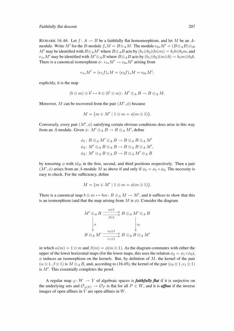
Faithfully flat descent 207

REMARK 16.46. Let f : A → B be a faithfully flat homomorphism, and let M be an A-module. WriteM ′ for theB-module f∗M = B⊗AM . The module e0∗M ′ = (B⊗AB)⊗BM ′ may be identified withB⊗AM ′ whereB⊗AB acts by (b1⊗b2)(b⊗m) = b1b⊗b2m, ande1∗M

′ may be identified withM ′⊗AB whereB⊗AB acts by (b1⊗b2)(m⊗b) = b1m⊗b2b.There is a canonical isomorphism φ : e1∗M ′ → e0∗M

′ arising from

e1∗M′ = (e1f)∗M = (e0f)∗M = e0∗M

′;

explicitly, it is the map

(b⊗m)⊗ b′ 7→ b⊗ (b′ ⊗m) : M ′ ⊗A B → B ⊗AM.

Moreover, M can be recovered from the pair (M ′, φ) because

M = m ∈M ′ | 1⊗m = φ(m⊗ 1).

Conversely, every pair (M ′, φ) satisfying certain obvious conditions does arise in this wayfrom an A-module. Given φ : M ′ ⊗A B → B ⊗AM ′, define

φ1 : B ⊗AM ′ ⊗A B → B ⊗A B ⊗AM ′

φ2 : M ′ ⊗A B ⊗A B → B ⊗A B ⊗AM ′,

φ3 : M ′ ⊗A B ⊗A B → B ⊗AM ′ ⊗A B

by tensoring φ with idB in the first, second, and third positions respectively. Then a pair(M ′, φ) arises from an A-module M as above if and only if φ2 = φ1 φ3. The necessity iseasy to check. For the sufficiency, define

M = m ∈M ′ | 1⊗m = φ(m⊗ 1).

There is a canonical map b ⊗m 7→ bm : B ⊗AM → M ′, and it suffices to show that thisis an isomorphism (and that the map arising from M is φ). Consider the diagram

M ′ ⊗A Bα⊗1

>

β⊗1> B ⊗AM ′ ⊗A B

B ⊗AM ′

φ

∨ e0⊗1>

e1⊗1> B ⊗A B ⊗AM ′

φ1

∨

in which α(m) = 1⊗m and β(m) = φ(m⊗ 1). As the diagram commutes with either theupper of the lower horizontal maps (for the lower maps, this uses the relation φ2 = φ1φ3),φ induces an isomorphism on the kernels. But, by defintion of M , the kernel of the pair(α⊗ 1, β⊗ 1) is M ⊗AB, and, according to (16.45), the kernel of the pair (e0⊗ 1, e1⊗ 1)is M ′. This essentially completes the proof.

A regular map ϕ : W → V of algebraic spaces is faithfully flat if it is surjective onthe underlying sets and Oϕ(P ) → OP is flat for all P ∈ W , and it is affine if the inverseimages of open affines in V are open affines in W .

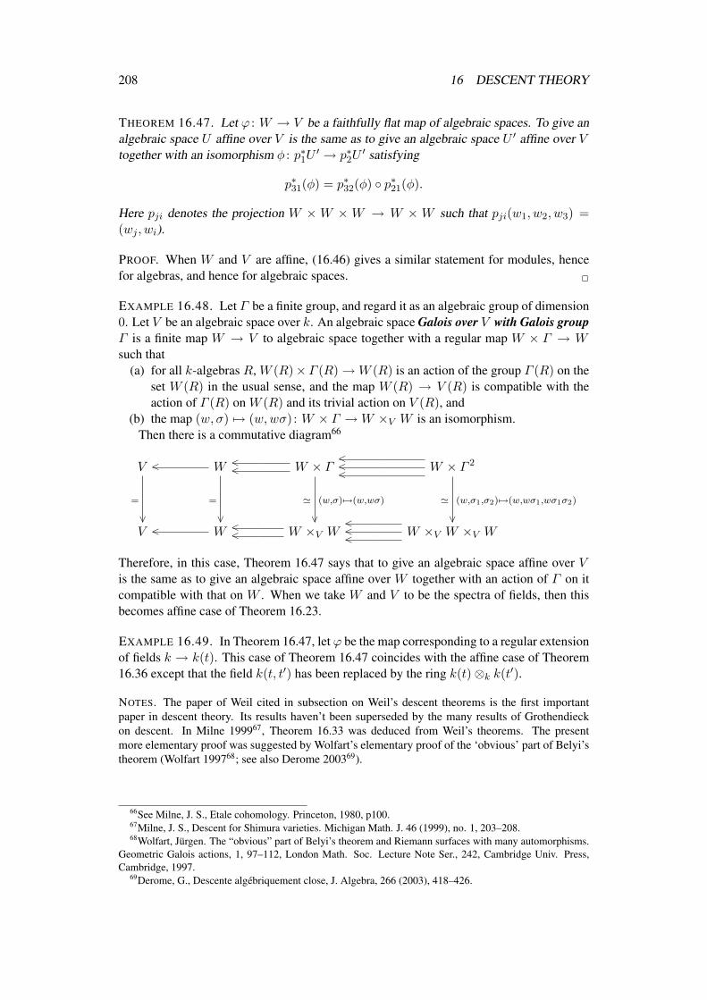
208 16 DESCENT THEORY

THEOREM 16.47. Let ϕ : W → V be a faithfully flat map of algebraic spaces. To give analgebraic space U affine over V is the same as to give an algebraic space U ′ affine over Vtogether with an isomorphism φ : p∗1U

′ → p∗2U′ satisfying

p∗31(φ) = p∗32(φ) p∗21(φ).

Here pji denotes the projection W × W × W → W × W such that pji(w1, w2, w3) =(wj , wi).

PROOF. When W and V are affine, (16.46) gives a similar statement for modules, hencefor algebras, and hence for algebraic spaces. 2

EXAMPLE 16.48. Let Γ be a finite group, and regard it as an algebraic group of dimension0. Let V be an algebraic space over k. An algebraic space Galois over V with Galois groupΓ is a finite map W → V to algebraic space together with a regular map W × Γ → Wsuch that

(a) for all k-algebras R, W (R)× Γ (R)→W (R) is an action of the group Γ (R) on theset W (R) in the usual sense, and the map W (R) → V (R) is compatible with theaction of Γ (R) on W (R) and its trivial action on V (R), and

(b) the map (w, σ) 7→ (w,wσ) : W × Γ →W ×V W is an isomorphism.Then there is a commutative diagram66

V < W << W × Γ

<<<

W × Γ 2

V

=

∨< W

=

∨<< W ×V W

' (w,σ) 7→(w,wσ)

∨ <<<

W ×V W ×V W

' (w,σ1,σ2) 7→(w,wσ1,wσ1σ2)

∨

Therefore, in this case, Theorem 16.47 says that to give an algebraic space affine over Vis the same as to give an algebraic space affine over W together with an action of Γ on itcompatible with that on W . When we take W and V to be the spectra of fields, then thisbecomes affine case of Theorem 16.23.

EXAMPLE 16.49. In Theorem 16.47, let ϕ be the map corresponding to a regular extensionof fields k → k(t). This case of Theorem 16.47 coincides with the affine case of Theorem16.36 except that the field k(t, t′) has been replaced by the ring k(t)⊗k k(t′).

NOTES. The paper of Weil cited in subsection on Weil’s descent theorems is the first importantpaper in descent theory. Its results haven’t been superseded by the many results of Grothendieckon descent. In Milne 199967, Theorem 16.33 was deduced from Weil’s theorems. The presentmore elementary proof was suggested by Wolfart’s elementary proof of the ‘obvious’ part of Belyi’stheorem (Wolfart 199768; see also Derome 200369).

66See Milne, J. S., Etale cohomology. Princeton, 1980, p100.67Milne, J. S., Descent for Shimura varieties. Michigan Math. J. 46 (1999), no. 1, 203–208.68Wolfart, Jurgen. The “obvious” part of Belyi’s theorem and Riemann surfaces with many automorphisms.

Geometric Galois actions, 1, 97–112, London Math. Soc. Lecture Note Ser., 242, Cambridge Univ. Press,Cambridge, 1997.

69Derome, G., Descente algebriquement close, J. Algebra, 266 (2003), 418–426.

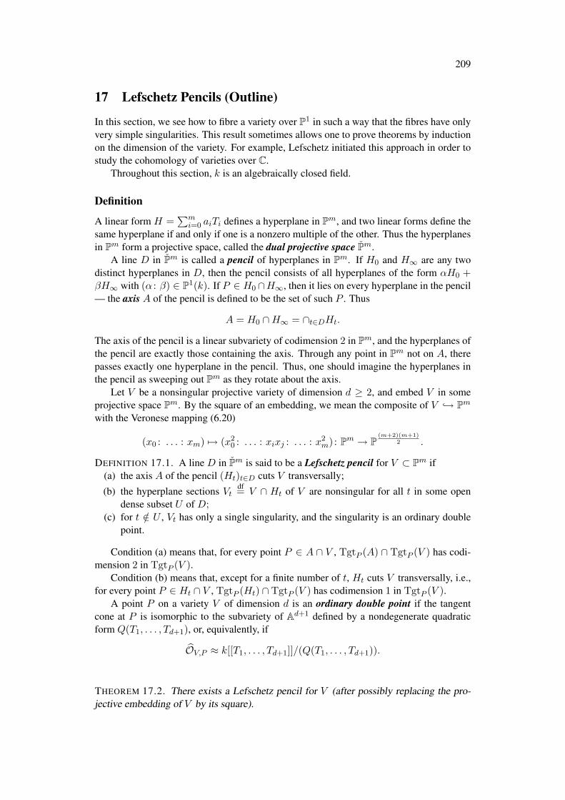
209

17 Lefschetz Pencils (Outline)

In this section, we see how to fibre a variety over P1 in such a way that the fibres have onlyvery simple singularities. This result sometimes allows one to prove theorems by inductionon the dimension of the variety. For example, Lefschetz initiated this approach in order tostudy the cohomology of varieties over C.

Throughout this section, k is an algebraically closed field.

Definition

A linear form H =∑m

i=0 aiTi defines a hyperplane in Pm, and two linear forms define thesame hyperplane if and only if one is a nonzero multiple of the other. Thus the hyperplanesin Pm form a projective space, called the dual projective space Pm.

A line D in Pm is called a pencil of hyperplanes in Pm. If H0 and H∞ are any twodistinct hyperplanes in D, then the pencil consists of all hyperplanes of the form αH0 +βH∞ with (α : β) ∈ P1(k). If P ∈ H0 ∩H∞, then it lies on every hyperplane in the pencil— the axis A of the pencil is defined to be the set of such P . Thus

A = H0 ∩H∞ = ∩t∈DHt.

The axis of the pencil is a linear subvariety of codimension 2 in Pm, and the hyperplanes ofthe pencil are exactly those containing the axis. Through any point in Pm not on A, therepasses exactly one hyperplane in the pencil. Thus, one should imagine the hyperplanes inthe pencil as sweeping out Pm as they rotate about the axis.

Let V be a nonsingular projective variety of dimension d ≥ 2, and embed V in someprojective space Pm. By the square of an embedding, we mean the composite of V → Pmwith the Veronese mapping (6.20)

(x0 : . . . : xm) 7→ (x20 : . . . : xixj : . . . : x2

m) : Pm → P(m+2)(m+1)

2 .

DEFINITION 17.1. A line D in Pm is said to be a Lefschetz pencil for V ⊂ Pm if(a) the axis A of the pencil (Ht)t∈D cuts V transversally;

(b) the hyperplane sections Vtdf= V ∩ Ht of V are nonsingular for all t in some open

dense subset U of D;(c) for t /∈ U , Vt has only a single singularity, and the singularity is an ordinary double

point.

Condition (a) means that, for every point P ∈ A ∩ V , TgtP (A) ∩ TgtP (V ) has codi-mension 2 in TgtP (V ).

Condition (b) means that, except for a finite number of t, Ht cuts V transversally, i.e.,for every point P ∈ Ht ∩ V , TgtP (Ht) ∩ TgtP (V ) has codimension 1 in TgtP (V ).

A point P on a variety V of dimension d is an ordinary double point if the tangentcone at P is isomorphic to the subvariety of Ad+1 defined by a nondegenerate quadraticform Q(T1, . . . , Td+1), or, equivalently, if

OV,P ≈ k[[T1, . . . , Td+1]]/(Q(T1, . . . , Td+1)).

THEOREM 17.2. There exists a Lefschetz pencil for V (after possibly replacing the pro-jective embedding of V by its square).

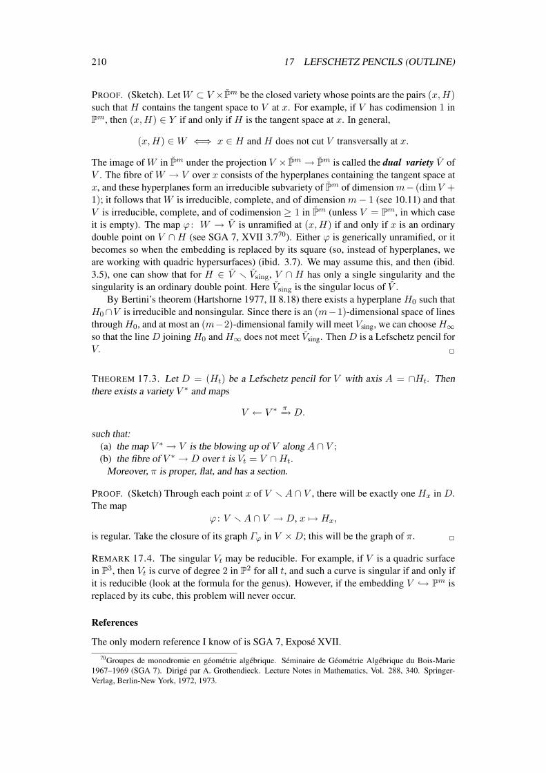
210 17 LEFSCHETZ PENCILS (OUTLINE)

PROOF. (Sketch). LetW ⊂ V ×Pm be the closed variety whose points are the pairs (x,H)such that H contains the tangent space to V at x. For example, if V has codimension 1 inPm, then (x,H) ∈ Y if and only if H is the tangent space at x. In general,

(x,H) ∈W ⇐⇒ x ∈ H and H does not cut V transversally at x.

The image of W in Pm under the projection V × Pm → Pm is called the dual variety V ofV . The fibre of W → V over x consists of the hyperplanes containing the tangent space atx, and these hyperplanes form an irreducible subvariety of Pm of dimension m− (dimV +1); it follows that W is irreducible, complete, and of dimension m− 1 (see 10.11) and thatV is irreducible, complete, and of codimension ≥ 1 in Pm (unless V = Pm, in which caseit is empty). The map ϕ : W → V is unramified at (x,H) if and only if x is an ordinarydouble point on V ∩H (see SGA 7, XVII 3.770). Either ϕ is generically unramified, or itbecomes so when the embedding is replaced by its square (so, instead of hyperplanes, weare working with quadric hypersurfaces) (ibid. 3.7). We may assume this, and then (ibid.3.5), one can show that for H ∈ V r Vsing, V ∩ H has only a single singularity and thesingularity is an ordinary double point. Here Vsing is the singular locus of V .

By Bertini’s theorem (Hartshorne 1977, II 8.18) there exists a hyperplane H0 such thatH0∩V is irreducible and nonsingular. Since there is an (m−1)-dimensional space of linesthroughH0, and at most an (m−2)-dimensional family will meet Vsing, we can chooseH∞so that the line D joining H0 and H∞ does not meet Vsing. Then D is a Lefschetz pencil forV. 2

THEOREM 17.3. Let D = (Ht) be a Lefschetz pencil for V with axis A = ∩Ht. Thenthere exists a variety V ∗ and maps

V ← V ∗ π−→ D.

such that:(a) the map V ∗ → V is the blowing up of V along A ∩ V ;(b) the fibre of V ∗ → D over t is Vt = V ∩Ht.

Moreover, π is proper, flat, and has a section.

PROOF. (Sketch) Through each point x of V r A ∩ V , there will be exactly one Hx in D.The map

ϕ : V rA ∩ V → D, x 7→ Hx,

is regular. Take the closure of its graph Γϕ in V ×D; this will be the graph of π. 2

REMARK 17.4. The singular Vt may be reducible. For example, if V is a quadric surfacein P3, then Vt is curve of degree 2 in P2 for all t, and such a curve is singular if and only ifit is reducible (look at the formula for the genus). However, if the embedding V → Pm isreplaced by its cube, this problem will never occur.

References

The only modern reference I know of is SGA 7, Expose XVII.70Groupes de monodromie en geometrie algebrique. Seminaire de Geometrie Algebrique du Bois-Marie

1967–1969 (SGA 7). Dirige par A. Grothendieck. Lecture Notes in Mathematics, Vol. 288, 340. Springer-Verlag, Berlin-New York, 1972, 1973.

211

18 Algebraic Schemes

In this course, we have attached an affine algebraic variety to any algebra of finite typeover a field k. For many reasons, for example, in order to be able to study the reductionof varieties to characteristic p 6= 0, Grothendieck realized that it is important to attach ageometric object to every commutative ring. Unfortunately, A 7→ spmA is not functorialin this generality: if ϕ : A→ B is a homomorphism of rings, then ϕ−1(m) for m maximalneed not be maximal — consider for example the inclusion Z → Q. Thus he was forced toreplace spm(A) with spec(A), the set of all prime ideals in A. He then attaches an affinescheme Spec(A) to each ring A, and defines a scheme to be a locally ringed space thatadmits an open covering by affine schemes.

There is a natural functor V 7→ V ∗ from the category of algebraic spaces over k tothe category of schemes of finite-type over k, which is an equivalence of categories. Thealgebraic varieties correspond to geometrically reduced schemes. To construct V ∗ from V ,one only has to add one point for each irreducible closed subvariety of V . The topology issuch that U 7→ U∗ is a bijection from the set of open subsets of V to the set of open subsetsof V ∗. Moreover, Γ (U∗,OV ∗) = Γ (U,OV ) for each open subset U of V . Therefore thetopologies and sheaves on V and V ∗ are the same — only the underlying sets differ.71

Every aspiring algebraic and (especially) arithmetic geometer needs to learn the basictheory of schemes, and for this I recommend reading Chapters II and III of Hartshorne1997.

71Some authors call a geometrically reduced scheme of finite-type over a field a variety. Despite theirsimilarity, it is important to distinguish such schemes from varieties (in the sense of these notes). Forexample, if W and W ′ are subvarieties of a variety, their intersection in the sense of schemes neednot be reduced, and so may differ from their intersection in the sense of varieties. For example, ifW = V (a) ⊂ An and W ′ = V (a′) ⊂ An′

with a and a′ radical, then the intersection W andW ′ in the sense of schemes is Spec k[X1, . . . , Xn+n′ ]/(a, a′) while their intersection in the sense ofvarieties is Spec k[X1, . . . , Xn+n′ ]/rad(a, a′) (and their intersection in the sense of algebraic spaces isSpm k[X1, . . . , Xn+n′ ]/(a, a′).

212 A SOLUTIONS TO THE EXERCISES

A Solutions to the exercises

1-1 Use induction on n. For n = 1, use that a nonzero polynomial in one variable has onlyfinitely many roots (which follows from unique factorization, for example). Now supposen > 1 and write f =

∑giX

in with each gi ∈ k[X1, . . . , Xn−1]. If f is not the zero

polynomial, then some gi is not the zero polynomial. Therefore, by induction, there exist(a1, . . . , an−1) ∈ kn−1 such that f(a1, . . . , an−1, Xn) is not the zero polynomial. Now, bythe degree-one case, there exists a b such that f(a1, . . . , an−1, b) 6= 0.

1-2 (X + 2Y, Z); Gaussian elimination (to reduce the matrix of coefficients to row echelonform); (1), unless the characteristic of k is 2, in which case the ideal is (X + 1, Z + 1).

2-1 W = Y -axis, and so I(W ) = (X). Clearly,

(X2, XY 2) ⊂ (X) ⊂ rad(X2, XY 2)

and rad((X)) = (X). On taking radicals, we find that (X) = rad(X2, XY 2).

2-2 The d× d minors of a matrix are polynomials in the entries of the matrix, and the set ofmatrices with rank ≤ r is the set where all (r + 1)× (r + 1) minors are zero.

2-3 Clearly V = V (Xn −Xn1 , . . . , X2 −X2

1 ). The map

Xi 7→ T i : k[X1, . . . , Xn]→ k[T ]

induces an isomorphism k[V ] → A1. [Hence t 7→ (t, . . . , tn) is an isomorphism of affinevarieties A1 → V .]

2-4 We use that the prime ideals are in one-to-one correspondence with the closed irre-ducible subsets Z of A2. For such a set, 0 ≤ dimZ ≤ 2.

Case dimZ = 2. Then Z = A2, and the corresponding ideal is (0).Case dimZ = 1. Then Z 6= A2, and so I(Z) contains a nonzero polynomial f(X,Y ).

If I(Z) 6= (f), then dimZ = 0 by (2.25, 2.26). Hence I(Z) = (f).Case dimZ = 0. Then Z is a point (a, b) (see 2.24c), and so I(Z) = (X − a, Y − b).

2-5 The statement Homk−algebras(A ⊗Q k,B ⊗Q k) 6= ∅ can be interpreted as saying thata certain set of polynomials has a zero in k. If the polynomials have a common zero inC, then the ideal they generate in C[X1, . . .] does not contain 1. A fortiori the ideal theygenerate in k[X1, . . .] does not contain 1, and so the Nullstellensatz (2.6) implies that thepolynomials have a common zero in k.

3-1 A map α : A1 → A1 is continuous for the Zariski topology if the inverse images offinite sets are finite, whereas it is regular only if it is given by a polynomial P ∈ k[T ], so itis easy to give examples, e.g., any map α such that α−1(point) is finite but arbitrarily large.

3-2 The argument in the text shows that, for any f ∈ S,

f(a1, . . . , an) = 0 =⇒ f(aq1, . . . , aqn) = 0.

This implies that ϕ maps V into itself, and it is obviously regular because it is defined bypolynomials.

3-3 The image omits the points on the Y -axis except for the origin. The complement of theimage is not dense, and so it is not open, but any polynomial zero on it is also zero at (0, 0),and so it not closed.

213

3-5 No, because both +1 and −1 map to (0, 0). The map on rings is

k[x, y]→ k[T ], x 7→ T 2 − 1, y 7→ T (T 2 − 1),

which is not surjective (T is not in the image).

4-1 Let f be regular on P1. Then f |U0 = P (X) ∈ k[X], where X is the regular function(a0 : a1) 7→ a1/a0 : U0 → k, and f |U1 = Q(Y ) ∈ k[Y ], where Y is (a0 : a1) 7→ a0/a1.On U0 ∩ U1, X and Y are reciprocal functions. Thus P (X) and Q(1/X) define the samefunction on U0 ∩ U1 = A1 r 0. This implies that they are equal in k(X), and must bothbe constant.

4-2 Note that Γ (V,OV ) =∏Γ (Vi,OVi) — to give a regular function on

⊔Vi is the same

as to give a regular function on each Vi (this is the “obvious” ringed space structure).Thus, if V is affine, it must equal Specm(

∏Ai), where Ai = Γ (Vi,OVi), and so V =⊔

Specm(Ai) (use the description of the ideals in A×B on p6). Etc..

4-3 Let H be an algebraic subgroup of G. By definition, H is locally closed, i.e., open inits Zariski closure H . Assume first that H is connected. Then H is a connected algebraicgroup, and it is a disjoint union of the cosets of H . It follows that H = H . In the generalcase, H is a finite disjoint union of its connected components; as one component is closed,they all are.

5-1 (b) The singular points are the common solutions to4X3 − 2XY 2 = 0 =⇒ X = 0 or Y 2 = 2X2

4Y 3 − 2X2Y = 0 =⇒ Y = 0 or X2 = 2Y 2

X4 + Y 4 −X2Y 2 = 0.

Thus, only (0, 0) is singular, and the variety is its own tangent cone.

5-2 Directly from the definition of the tangent space, we have that

Ta(V ∩H) ⊂ Ta(V ) ∩ Ta(H).

AsdimTa(V ∩H) ≥ dimV ∩H = dimV − 1 = dimTa(V ) ∩ Ta(H),

we must have equalities everywhere, which proves that a is nonsingular on V ∩ H . (Inparticular, it can’t lie on more than one irreducible component.)

The surface Y 2 = X2+Z is smooth, but its intersection with theX-Y plane is singular.No, P needn’t be singular on V ∩ H if H ⊃ TP (V ) — for example, we could have

H ⊃ V or H could be the tangent line to a curve.

5-3 We can assume V and W to affine, say

I(V ) = a ⊂ k[X1, . . . , Xm]I(W ) = b ⊂ k[Xm+1, . . . , Xm+n].

If a = (f1, . . . , fr) and b = (g1, . . . , gs), then I(V ×W ) = (f1, . . . , fr, g1, . . . , gs). Thus,T(a,b)(V ×W ) is defined by the equations

(df1)a = 0, . . . , (dfr)a = 0, (dg1)b = 0, . . . , (dgs)b = 0,

214 A SOLUTIONS TO THE EXERCISES

which can obviously be identified with Ta(V )× Tb(W ).

5-4 Take C to be the union of the coordinate axes in An. (Of course, if you want C to beirreducible, then this is more difficult. . . )

5-5 A matrix A satisfies the equations

(I + εA)tr · J · (I + εA) = I

if and only ifAtr · J + J ·A = 0.

Such an A is of the form(M NP Q

)with M,N,P,Q n× n-matrices satisfying

N tr = N, P tr = P, M tr = −Q.

The dimension of the space of A’s is therefore

n(n+ 1)2

(for N ) +n(n+ 1)

2(for P ) + n2 (for M,Q) = 2n2 + n.

5-6 Let C be the curve Y 2 = X3, and consider the map A1 → C, t 7→ (t2, t3). Thecorresponding map on rings k[X,Y ]/(Y 2)→ k[T ] is not an isomorphism, but the map onthe geometric tangent cones is an isomorphism.

5-7 The singular locus Vsing has codimension ≥ 2 in V , and this implies that V is normal.[Idea of the proof: let f ∈ k(V ) be integral over k[V ], f /∈ k[V ], f = g/h, g, h ∈ k[V ];for any P ∈ V (h) r V (g), OP is not integrally closed, and so P is singular.]

5-8 No! Let a = (X2Y ). Then V (a) is the union of theX and Y axes, and IV (a) = (XY ).For a = (a, b),

(dX2Y )a = 2ab(X − a) + a2(Y − b)(dXY )a = b(X − a) + a(Y − b).

If a 6= 0 and b = 0, then the equations

(dX2Y )a = a2Y = 0(dXY )a = aY = 0

have the same solutions.

6-1 Let P = (a : b : c), and assume c 6= 0. Then the tangent line at P = (ac : bc : 1) is(

∂F

∂X

)P

X +(∂F

∂Y

)P

Y −((

∂F

∂X

)P

(ac

)+(∂F

∂Y

)P

(b

c

))Z = 0.

Now use that, because F is homogeneous,

F (a, b, c) = 0 =⇒(∂F

∂X

)P

a+(∂F

∂Y

)P

+(∂F

∂Z

)P

c = 0.

(This just says that the tangent plane at (a, b, c) to the affine cone F (X,Y, Z) = 0 passesthrough the origin.) The point at∞ is (0 : 1 : 0), and the tangent line is Z = 0, the line at

215

∞. [The line at∞meets the cubic curve at only one point instead of the expected 3, and sothe line at∞ “touches” the curve, and the point at∞ is a point of inflexion.]

6-2 The equation defining the conic must be irreducible (otherwise the conic is singular).After a linear change of variables, the equation will be of the form X2 + Y 2 = Z2 (thisis proved in calculus courses). The equation of the line in aX + bY = cZ, and the rest iseasy. [Note that this is a special case of Bezout’s theorem (6.34) because the multiplicity is2 in case (b).]

6-3 (a) The ring

k[X,Y, Z]/(Y −X2, Z −X3) = k[x, y, z] = k[x] ' k[X],

which is an integral domain. Therefore, (Y −X2, Z −X3) is a radical ideal.(b) The polynomial F = Z − XY = (Z − X3) − X(Y − X2) ∈ I(V ) and F ∗ =

ZW −XY . IfZW −XY = (YW −X2)f + (ZW 2 −X3)g,

then, on equating terms of degree 2, we would find

ZW −XY = a(YW −X2),

which is false.

6-4 Let P = (a0 : . . . : an) and Q = (b0 : . . . : bn) be two points of Pn, n ≥ 2. Thecondition that the hyperplane Lc :

∑ciXi = 0 pass through P and not through Q is that∑

aici = 0,∑bici 6= 0.

The (n + 1)-tuples (c0, . . . , cn) satisfying these conditions form a nonempty open subsetof the hyperplane H :

∑aiXi = 0 in An+1. On applying this remark to the pairs (P0, Pi),

we find that the (n+ 1)-tuples c = (c0, . . . , cn) such that P0 lies on the hyperplane Lc butnot P1, . . . , Pr form a nonempty open subset of H .

6-5 The subsetC = (a : b : c) | a 6= 0, b 6= 0 ∪ (1 : 0 : 0)

of P2 is not locally closed. Let P = (1 : 0 : 0). If the set C were locally closed, then Pwould have an open neighbourhood U in P2 such that U ∩ C is closed. When we look inU0, P becomes the origin, and

C ∩ U0 = (A2 r X-axis) ∪ origin.

The open neighbourhoods U of P are obtained by removing from A2 a finite number ofcurves not passing through P . It is not possible to do this in such a way that U ∩C is closedin U (U ∩C has dimension 2, and so it can’t be a proper closed subset of U ; we can’t haveU ∩ C = U because any curve containing all nonzero points on X-axis also contains theorigin).

7-2 Define f(v) = h(v,Q) and g(w) = h(P,w), and let ϕ = h − (f p + g q). Thenϕ(v,Q) = 0 = ϕ(P,w), and so the rigidity theorem (7.13) implies that ϕ is identicallyzero.

216 A SOLUTIONS TO THE EXERCISES

6-6 Let∑cijXij = 0 be a hyperplane containing the image of the Segre map. We then

have ∑cijaibj = 0

for all a = (a0, . . . , am) ∈ km+1 and b = (b0, . . . , bn) ∈ kn+1. In other words,

aCbt = 0

for all a ∈ km+1 and b ∈ kn+1, where C is the matrix (cij). This equation shows thataC = 0 for all a, and this implies that C = 0.

8-2 For example, consider

(A1 r 1)→ A1 x 7→xn

→ A1

for n > 1 an integer prime to the characteristic. The map is obviously quasi-finite, but it isnot finite because it corresponds to the map of k-algebras

X 7→ Xn : k[X]→ k[X, (X − 1)−1]

which is not finite (the elements 1/(X−1)i, i ≥ 1, are linearly independent over k[X], andso also over k[Xn]).

8-3 Assume that V is separated, and consider two regular maps f, g : Z ⇒ W . We have toshow that the set on which f and g agree is closed in Z. The set where ϕf and ϕg agreeis closed in Z, and it contains the set where f and g agree. Replace Z with the set whereϕ f and ϕ g agree. Let U be an open affine subset of V , and let Z ′ = (ϕ f)−1(U) =(ϕ g)−1(U). Then f(Z ′) and g(Z ′) are contained in ϕ−1(U), which is an open affinesubset of W , and is therefore separated. Hence, the subset of Z ′ on which f and g agree isclosed. This proves the result.

[Note that the problem implies the following statement: if ϕ : W → V is a finite regularmap and V is separated, then W is separated.]

8-4 Let V = An, and let W be the subvariety of An × A1 defined by the polynomial∏ni=1(X − Ti) = 0.

The fibre over (t1, . . . , tn) ∈ An is the set of roots of∏

(X − ti). Thus, Vn = An; Vn−1 isthe union of the linear subspaces defined by the equations

Ti = Tj , 1 ≤ i, j ≤ n, i 6= j;

Vn−2 is the union of the linear subspaces defined by the equations

Ti = Tj = Tk, 1 ≤ i, j, k ≤ n, i, j, k distinct,

and so on.

10-1 Consider an orbit O = Gv. The map g 7→ gv : G → O is regular, and so O containsan open subset U of O (10.2). If u ∈ U , then gu ∈ gU , and gU is also a subset of Owhich is open in O (because P 7→ gP : V → V is an isomorphism). Thus O, regarded asa topological subspace of O, contains an open neighbourhood of each of its points, and somust be open in O.

217

We have shown that O is locally closed in V , and so has the structure of a subvariety.From (5.18), we know that it contains at least one nonsingular point P . But then gP isnonsingular, and every point of O is of this form.

From set theory, it is clear that O r O is a union of orbits. Since O r O is a properclosed subset of O, all of its subvarieties must have dimension < dimO = dimO.

Let O be an orbit of lowest dimension. The last statement implies that O = O.

10-2 An orbit of type (a) is closed, because it is defined by the equations

Tr(A) = −a, det(A) = b,

(as a subvariety of V ). It is of dimension 2, because the centralizer of(α 00 β

), α 6= β, is(

∗ 00 ∗

), which has dimension 2.

An orbit of type (b) is of dimension 2, but is not closed: it is defined by the equations

Tr(A) = −a, det(A) = b, A 6=(α 00 α

), α = root of X2 + aX + b.

An orbit of type (c) is closed of dimension 0: it is defined by the equationA =(α 00 α

).

An orbit of type (b) contains an orbit of type (c) in its closure.

10-3 Let ζ be a primitive dth root of 1. Then, for each i, j, 1 ≤ i, j ≤ d, the followingequations define lines on the surface

X0 + ζiX1 = 0X2 + ζjX3 = 0

X0 + ζiX2 = 0X1 + ζjX3 = 0

X0 + ζiX3 = 0X1 + ζjX2 = 0.

There are three sets of lines, each with d2 lines, for a total of 3d2 lines.

10-4 (a) Compare the proof of Theorem 10.9.(b) Use the transitivity, and apply Proposition 8.24.

12-1 LetH be a hyperplane in Pn intersecting V transversally. ThenH ≈ Pn−1 and V ∩His again defined by a polynomial of degree δ. Continuing in this fashion, we find that

V ∩H1 ∩ . . . ∩Hd

is isomorphic to a subset of P1 defined by a polynomial of degree δ.

12-2 We may suppose that X is not a factor of Fm, and then look only at the affine piece ofthe blow-up, σ : A2 → A2, (x, y) 7→ (x, xy). Then σ−1(C r (0, 0))is given by equations

X 6= 0, F (X,XY ) = 0.

ButF (X,XY ) = Xm(

∏(ai − biY )ri) +Xm+1Fm+1(X,Y ) + · · · ,

and so σ−1(C r (0, 0)) is also given by equations

X 6= 0,∏

(ai − biY )ri +XFm+1(X,Y ) + · · · = 0.

218 A SOLUTIONS TO THE EXERCISES

To find its closure, drop the condition X 6= 0. It is now clear that the closure intersectsσ−1(0, 0) (the Y -axis) at the s points Y = ai/bi.

12-3 We have to find the dimension of k[X,Y ](X,Y )/(Y 2 − Xr, Y 2 − Xs). In this ring,Xr = Xs, and so Xs(Xr−s − 1) = 0. As Xr−s − 1 is a unit in the ring, this implies thatXs = 0, and it follows that Y 2 = 0. Thus (Y 2 −Xr, Y 2 −Xs) ⊃ (Y 2, Xs), and in factthe two ideals are equal in k[X,Y ](X,Y ). It is now clear that the dimension is 2s.

12-4 Note thatk[V ] = k[T 2, T 3] =

∑aiT

i | ai = 0.

For each a ∈ k, define an effective divisor Da on V as follows:Da has local equation 1− a2T 2 on the set where 1 + aT 6= 0;Da has local equation 1− a3T 3 on the set where 1 + aT + aT 2 6= 0.

The equations

(1− aT )(1 + aT ) = 1− a2T 2, (1− aT )(1 + aT + a2T 2) = 1− a3T 3

show that the two divisors agree on the overlap where

(1 + aT )(1 + aT + aT 2) 6= 0.

For a 6= 0, Da is not principal, essentially because

gcd(1− a2T 2, 1− a3T 3) = (1− aT ) /∈ k[T 2, T 3]

— if Da were principal, it would be a divisor of a regular function on V , and that regularfunction would have to be 1− aT , but this is not allowed.

In fact, one can show that Pic(V ) ≈ k. Let V ′ = V r (0, 0), and write P (∗) for theprincipal divisors on ∗. Then Div(V ′) + P (V ) = Div(V ), and so

Div(V )/P (V ) ' Div(V ′)/Div(V ′) ∩ P (V ) ' P (V ′)/P (V ′) ∩ P (V ) ' k.

219

B Annotated Bibliography

Apart from Hartshorne 1977, among the books listed below, I especially recommend Sha-farevich 1994 — it is very easy to read, and is generally more elementary than these notes,but covers more ground (being much longer).

Commutative AlgebraAtiyah, M.F and MacDonald, I.G., Introduction to Commutative Algebra, Addison-Wesley

1969. This is the most useful short text. It extracts the essence of a good part of Bourbaki1961–83.

Bourbaki, N., Algebre Commutative, Chap. 1–7, Hermann, 1961–65; Chap 8–9, Masson,1983. Very clearly written, but it is a reference book, not a text book.

Eisenbud, D., Commutative Algebra, Springer, 1995. The emphasis is on motivation.Matsumura, H., Commutative Ring Theory, Cambridge 1986. This is the most useful medium-

length text (but read Atiyah and MacDonald or Reid first).Nagata, M., Local Rings, Wiley, 1962. Contains much important material, but it is concise to

the point of being almost unreadable.Reid, M., Undergraduate Commutative Algebra, Cambridge 1995. According to the author, it

covers roughly the same material as Chapters 1–8 of Atiyah and MacDonald 1969, but ischeaper, has more pictures, and is considerably more opinionated. (However, Chapters 10and 11 of Atiyah and MacDonald 1969 contain crucial material.)

Serre: Algebre Locale, Multiplicites, Lecture Notes in Math. 11, Springer, 1957/58 (thirdedition 1975).

Zariski, O., and Samuel, P., Commutative Algebra, Vol. I 1958, Vol II 1960, van Nostrand.Very detailed and well organized.

Elementary Algebraic GeometryAbhyankar, S., Algebraic Geometry for Scientists and Engineers, AMS, 1990. Mainly curves,

from a very explicit and down-to-earth point of view.Reid, M., Undergraduate Algebraic Geometry. A brief, elementary introduction. The fi-

nal section contains an interesting, but idiosyncratic, account of algebraic geometry in thetwentieth century.

Smith, Karen E.; Kahanpaa, Lauri; Kekalainen, Pekka; Traves, William. An invitation to alge-braic geometry. Universitext. Springer-Verlag, New York, 2000. An introductory overviewwith few proofs but many pictures.

Computational Algebraic GeometryCox, D., Little, J., O’Shea, D., Ideals, Varieties, and Algorithms, Springer, 1992. This gives

an algorithmic approach to algebraic geometry, which makes everything very down-to-earthand computational, but the cost is that the book doesn’t get very far in 500pp.

Subvarieties of Projective SpaceHarris, Joe: Algebraic Geometry: A first course, Springer, 1992. The emphasis is on exam-

ples.Musili, C. Algebraic geometry for beginners. Texts and Readings in Mathematics, 20. Hin-

dustan Book Agency, New Delhi, 2001.Shafarevich, I., Basic Algebraic Geometry, Book 1, Springer, 1994. Very easy to read.Algebraic Geometry over the Complex NumbersGriffiths, P., and Harris, J., Principles of Algebraic Geometry, Wiley, 1978. A comprehensive

study of subvarieties of complex projective space using heavily analytic methods.Mumford, D., Algebraic Geometry I: Complex Projective Varieties. The approach is mainly

algebraic, but the complex topology is exploited at crucial points.

220 B ANNOTATED BIBLIOGRAPHY

Shafarevich, I., Basic Algebraic Geometry, Book 3, Springer, 1994.Abstract Algebraic VarietiesDieudonne, J., Cours de Geometrie Algebrique, 2, PUF, 1974. A brief introduction to abstract

algebraic varieties over algebraically closed fields.Kempf, G., Algebraic Varieties, Cambridge, 1993. Similar approach to these notes, but is

more concisely written, and includes two sections on the cohomology of coherent sheaves.Kunz, E., Introduction to Commutative Algebra and Algebraic Geometry, Birkhauser, 1985.

Similar approach to these notes, but includes more commutative algebra and has a longchapter discussing how many equations it takes to describe an algebraic variety.

Mumford, D. Introduction to Algebraic Geometry, Harvard notes, 1966. Notes of a course.Apart from the original treatise (Grothendieck and Dieudonne 1960–67), this was the firstplace one could learn the new approach to algebraic geometry. The first chapter is onvarieties, and last two on schemes.

Mumford, David: The Red Book of Varieties and Schemes, Lecture Notes in Math. 1358,Springer, 1999. Reprint of Mumford 1966.

SchemesEisenbud, D., and Harris, J., Schemes: the language of modern algebraic geometry, Wadsworth,

1992. A brief elementary introduction to scheme theory.Grothendieck, A., and Dieudonne, J., Elements de Geometrie Algebrique. Publ. Math. IHES

1960–1967. This was intended to cover everything in algebraic geometry in 13 massivebooks, that is, it was supposed to do for algebraic geometry what Euclid’s “Elements” didfor geometry. Unlike the earlier Elements, it was abandoned after 4 books. It is an extremelyuseful reference.

Hartshorne, R., Algebraic Geometry, Springer 1977. Chapters II and III give an excellentaccount of scheme theory and cohomology, so good in fact, that no one seems willing towrite a competitor. The first chapter on varieties is very sketchy.

Iitaka, S. Algebraic Geometry: an introduction to birational geometry of algebraic varieties,Springer, 1982. Not as well-written as Hartshorne 1977, but it is more elementary, and itcovers some topics that Hartshorne doesn’t.

Shafarevich, I., Basic Algebraic Geometry, Book 2, Springer, 1994. A brief introduction toschemes and abstract varieties.

HistoryDieudonne, J., History of Algebraic Geometry, Wadsworth, 1985.Of Historical InterestHodge, W., and Pedoe, D., Methods of Algebraic Geometry, Cambridge, 1947–54.Lang, S., Introduction to Algebraic Geometry, Interscience, 1958. An introduction to Weil

1946.Weil, A., Foundations of Algebraic Geometry, AMS, 1946; Revised edition 1962. This is

where Weil laid the foundations for his work on abelian varieties and jacobian varietiesover arbitrary fields, and his proof of the analogue of the Riemann hypothesis for curvesand abelian varieties. Unfortunately, not only does its language differ from the currentlanguage of algebraic geometry, but it is incompatible with it.

Indexaction

continuous, 195, 205of a group on a vector space, 194regular, 204

affine algebra, 164algebra

finite, 4finitely generated, 4of finite-type, 4

algebraic group, 66algebraic space, 165

in the sense of Artin, 189axiom

separation, 59axis

of a pencil, 209

basic open subset, 37Bezout’s Theorem, 179birationally equivalent, 71

category, 20Chow group, 178codimension, 135complete intersection

ideal-theoretic, 140local, 140set-theoretic, 140

complex topology, 188cone

affine over a set, 99content of a polynomial, 9continuous

descent system, 196curve

elliptic, 29, 98, 101, 166, 183, 186cusp, 77cycle

algebraic, 178

degreeof a hypersurface, 115of a map, 150, 177of a point, 169of a projective variety, 117total, 10

derivation, 91descent datum, 196

effective, 196descent system, 196Dickson’s Lemma, 25differential, 78dimension, 70

Krull, 42of a reducible set, 40of an irreducible set, 40pure, 40, 71

division algorithm, 23divisor, 174

effective, 174local equation for, 175locally principal, 175positive, 174prime, 174principal, 174restriction of, 175support of, 174

domainunique factorization, 8

dual projective space, 209dual variety, 210

elementintegral over a ring, 11irreducible, 8

equivalence of categories, 21extension

of base field, 165of scalars, 165, 166of the base field, 166

fibregeneric, 200of a map, 127

fieldfixed, 191

field of rational functions, 40, 70form

leading, 76Frobenius map, 52function

rational, 47regular, 36, 44, 57

functor, 20contravariant, 20essentially surjective, 21fully faithful, 20

generate, 4germ

of a function, 44graph

of a regular map, 67Groebner basis, see standard basisgroup

symplectic, 96

221

222 INDEX

homogeneous, 104homomorphism

finite, 4of algebras, 4of presheaves, 160of sheaves, 160

hypersurface, 40, 109hypersurface section, 109

ideal, 4generated by a subset, 4homogeneous, 98maximal, 5monomial, 25prime, 4radical, 33

immersion, 61closed, 61open, 61

integral closure, 11intersect properly, 175, 176, 178irreducible components, 39isomorphic

locally, 93

leading coefficient, 23leading monomial, 23leading term, 23Lemma

Gauss’s, 8lemma

Nakayama’s, 6prime avoidance, 139Yoneda, 21Zariski’s, 32

linearly equivalent, 174local equation

for a divisor, 175local ring

regular, 7local system of parameters, 88

manifoldcomplex, 57differentiable, 57topological, 57

mapbirational, 131dominant, 54dominating, 54, 72etale, 81, 95finite, 126flat, 177quasi-finite, 127Segre, 110

separable, 152Veronese, 107

model, 166module

of differential one-forms, 186monomial, 10Morita equivalent, 195morphism

of affine algebraic varieties, 48of functors, 21of locally ringed spaces, 161of ringed spaces, 47, 161

multidegree, 23multiplicity

of a point, 77

neighbourhoodetale, 89

nilpotent, 33node, 77nondegenerate quadric, 156nonsingular, 170

orderinggrevlex, 23lex, 22

ordinary double point, 209

pencil, 209Lefschetz, 209

pencil of lines, 156perfect closure, 192Picard group, 174, 182Picard variety, 184point

multiple, 79nonsingular, 75, 79ordinary multiple, 77rational over a field, 169singular, 79smooth, 75, 79with coordinates in a field, 169with coordinates in a ring, 72

polynomialHilbert, 116homogeneous, 97primitive, 9

presheaf, 160prevariety, 165

algebraic, 57separated, 59

principal open subset, 37product

fibred, 69of algebraic varieties, 65

INDEX 223

of objects, 62tensor, 18

projection with centre, 110projectively normal, 174

quasi-inverse, 21

radicalof an ideal, 33

rationally equivalent, 178regular map, 58regulus, 156resultant, 121Riemann-Roch Theorem, 187ring

coordinate, 36integrally closed, 12noetherian, 6normal, 88of dual numbers, 91reduced, 33

ringed space, 43, 160locally, 160

section of a sheaf, 43semisimple

group, 93Lie algebra, 94

set(projective) algebraic, 97constructible, 144

sheaf, 160coherent, 180invertible, 182locally free, 180of abelian groups, 160of algebras, 43of k-algebras, 160of rings, 160support of, 180

singular locus, 76, 169specialization, 200splits

a descent system, 196stalk, 160standard basis, 26

minimal, 27reduced, 27

subring, 4subset

algebraic, 29multiplicative, 14

subspacelocally closed, 61

subvariety, 61

closed, 53open affine, 57

tangent cone, 77, 94geometric, 77, 94, 95

tangent space, 75, 78, 84theorem

Bezout’s , 115Chinese Remainder, 5going-up, 128Hilbert basis, 26, 30Hilbert Nullstellensatz, 31Krull’s principal ideal, 137Lefschetz pencils, 210Lefschetz pencils exist, 209Noether normalization, 130Stein factorization, 158strong Hilbert Nullstellensatz, 33Zariski’s main, 131

topological spaceirreducible , 37noetherian, 36quasicompact, 36

topologyetale, 89Krull, 197Zariski, 31

variety, 165abelian, 66, 123affine algebraic, 48algebraic, 59complete, 118flag, 114Grassmann, 112normal, 88, 174projective, 97quasi-projective, 97rational, 71unirational, 71