THE PUBLISHING HOUSE PROCEEDINGS OF THE ROMANIAN ACADEMY, Series A, OF THE ROMANIAN ACADEMY Volume 19, Number 3/2018, pp. 489–497

ALGEBRAIC MODELING OF KINEMATICS AND SINGULARITIES FOR A PROSTATE BIOPSY PARALLEL ROBOT

Doina PISLA1, Iosif BIRLESCU 1, Calin VAIDA1, Paul TUCAN 1, Adrian PISLA 1, Bogdan GHERMAN 1, Nicolae CRISAN 2, Nicolae PLITEA 1

1 Technical University Cluj-Napoca, Romania 2 “Iuliu Hatieganu” University of Medicine and Pharmacy, Cluj-Napoca, Romania

Corresponding author: Iosif BIRLESCU, E-mail: iosif.birlescu@mep.utcluj.ro

Abstract. The paper presents the mathematical modelling of the direct kinematics and singularities for a parallel robotic system designed for prostate biopsy. The mathematical description is obtained using Study parameters of SE(3) with quaternion representation. Based on the robot architecture and the active joint values, numerical solutions are presented for kinematics, and singularity conditions are obtained in the active joint space.

Key words: parallel robot, prostate biopsy, forward kinematics, singularity, study parameters.

1. INTRODUCTION

Prostate cancer has an increased risk factor among men [1, 2], and the rate of survival is correlated with the tumor staging (the survival rate in early stages is 99.9% and drops to 28% in later detection stages). As manual biopsies are carried in a blind way (based on current protocols), they often lead to false negative results. Thus, to enable cancer detection in early stages, accurate, targeted biopsies are required which leads to the introduction of robotics in such procedures [3]. For prostate biopsy, there are two ways of accessing the tissue, namely transperineal prostate biopsy (the needle is inserted into the prostate tissue through the patients perineum), and transrectal prostate biopsy (the needle is inserted through wall of the rectum into the prostate). A recent review published in Nature points out some advantages of the transperienal approach: it greatly reduces the risk of septicemia, it allows the sampling of the entire prostate (the apex is not reachable transrectaly) [4]. Moreover, medical imaging techniques are used (computerisez tomography, magnetic resonance imaging and transrectal ultrasonography) for targeted biopsies, to serve as procedure planning and real time intervention monitoring, with a variety of robotic structures used for biopsy and brachytherapy are synthetized into a document [5]. Novel robotic structures are also found in the literature, such as BIO-PROS 1 parallel robot for trasnsperineal prostate biopsy [6, 7]. A general mathematical method for solving kinematics and singularities is a vector method, with the problem of naturally occurring trigonometric functions in the equations, which may be substituted using the half tangent angle [8, 9, 10]. In some cases the kinematics may be determined even with experimental methods [11], based on advanced sensors used to capture and measure information that presents interest for monitoring and evaluating different kinematic or kinetic parameters of humans or robotic structures [12]. Study parameters of SE(3) is an algebraic method that proved to be an efficient in solving kinematic problems and describe singularities for closed loop mechanisms. The method was used to describe mechanisms, such as, the Stewart-Gough platform [8] and the 3-RPS manipulator [13], and it suggested more singularities than the vector method in the analysis of a brachytherapy robot [14, 15]. The goal of the paper is to determine a parametric mathematical description of the mechanism in polynomial form using Study parameters. This in turn leads to parametric characterization of the singular loci. By substituting the design parameters (e.g. lengths of the robot links) with numerical values the singularities are obtain for the proposed robotic structure, which will be implemented as a safety control function directly in the robot control. The paper is structured as follows: relevant mathematical

490 Doina PISLA, I. BIRLESCU, C. VAIDA, P. TUCAN, A.PISLA, B. GHERMAN, N. CRISAN, N. PLITEA 2

concepts are defined and explained in Section 2; Section 3 presents the BIO-PROS 1 robotic structure and the results of forward kinematic modelling, singularity analysis, and workspace generation; Section 4 treats conclusions and future research.

2. STUDY PARAMETERIZATION OF EUCLIDEAN DISPLACEMENT

To begin the mathematical description of the Study parameterization, the Euclidean displacement of a mobile frame X'(x',y',z')T, relative to a fixed frame X(x,y,z)T the matrix relation is used tXRX +⋅=' [8], where R’ is a 3 × 3 proper orthogonal matrix and t = [tx, ty, tz]T is a translation vector. A more convenient way to write the total Euclidean displacement is by using a 4 × 4 homogeneous transformation matrix (Eq. 1), where X’ and X have the form [1, x’, y’, z’]T and [1, x’, y’, z’]T and the Euclidean displacement ( tXRX +⋅=' ) is satisfied through 'X M X= ⋅ .

1 0

Mt R

=

(1)

By using the quaternion notation (with a quaternion X = x0+x1i+x2j+x3k) the proper orthogonal matrix R can be written as follows (xi being also called the Euler parameters) [8, 9]:

2 2 2 20 1 2 3 0 3 1 2 3 1 0 3

2 2 2 21 2 0 3 0 2 1 3 0 1 3 2

2 2 2 20 2 3 1 2 3 0 1 0 3 1 2

2( ) 2( )

2( ) 2( )

2( ) 2( )

x x x x x x x x x x x x

R x x x x x x x x x x x x

x x x x x x x x x x x x

+ − − − − +

= + + − − − − − − + + − −

. (2)

By introducing a second quaternion (Y = y0+y1i+y2j+y3k) and by accounting for the normalizing condition (x2

0+x21+x2

2+x23 = 1 which is a necessary condition for R to be a rotation matrix) and the Study quadric

(x0y0+x1y1+x2y2+x3y3 = 0) [8], the total Euclidean displacement may be written in the form of Eq. (1) with R in quaternion form and t(tx, ty, tz):

0 1 1 0 3 2 2 32( )xt x y x y x y x y= − − + (3) 0 2 2 0 1 3 3 12( )yt x y x y x y x y= − − + (4)

0 3 3 0 2 1 1 22( )zt x y x y x y x y= − − + . (5) The total Euclidean displacement may be written in the form x0:x1:x2:x3:y0:y1:y2:y3 which are called Study parameters [8], with the xi representing rotation parameters and the yi representing translation parameters:

0 1 2 3: : :x x x x = 122131132332332211 :::1 aaaaaaaaa −−−+++ 311312213322112332 ::1: aaaaaaaaa ++−−+− 322333221121123113 :1:: aaaaaaaaa +−+−+− 21 12 31 13 23 31 11 22 33: : :1a a a a a a a a a− + + − − +

(6)

0 1 2 3 1 2 3 0 3 2 3 0 1 2 1 01 1 1 1: : : ( ) : ( ) : ( ) : ( )2 2 2 2x y z x y z x y z x y zy y y y t x t x t x t x t x t x t x t x t x t x t x t x= + + − − + − − − + − . (7)

The aij terms in Eq. (6) are entries to a 3 × 3 orthogonal matrix (Eq. 2) were a11=x0+x1–x2–x3, a12=–2(x0x3-x1x2) and so on. To obtain solutions for Study parameters, algebraic geometry methods are used. Powerful

3 Algebraic modeling of kinematics and singularities for a prostate biopsy patallel robot 491

concepts such as ideals of varieties and Groebner bases are used in computing the kinematic and singularity problems, as they correspond to (projective) varieties in Study parameters space, and by adding the normalizing condition (x2

0+x21+x2

2+x23=1) the varieties become affine. This offers the opportunity to

compute the solutions for the forward kinematics and singularities using algebraic geometry methods as detailed in Section 3.

3. A PARALLEL ROBOTIC SYSTEM FOR PROSTATE BIOPSY

To perform the medical task, BIO-PROS 1 consists of two independent guiding modules: the needle guiding module, and the TRUS probe guiding module that will function as follows: the TRUS probe will be inserted through the patient rectum to enable real-time imaging of the prostate and the needle guiding module will insert the biopsy gun needle (using a specialised instrument with 1 redundant DOF) through the patient perineum and retrieve the tissue samples under the visual monitoring of the TRUS probe. Small needle angulation of about ±10° is required to allow the targeting of the entire prostate volume [3]. Regarding safety and reduced risk factor, the parallel architecture is proposed for increased precision and stability, while the large amplitude motion is not needed for the biopsy task.

3.1. MECHANISM DESCRIPTION

A schematic representation of BIO-PROS 1 robotic system and its' relative position with respect to the patient, is illustrated in Fig. 1 [7]. The 2 independent modules, have 5-DOF each, with the rotation around the longitudinal axis of the instrument (biopsy gun and TRUS probe) suppressed.

Fig. 1 – BIO-PROS 1 robotic system for transperineal prostate biopsy.

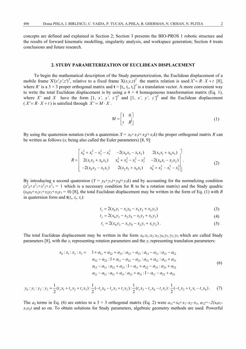
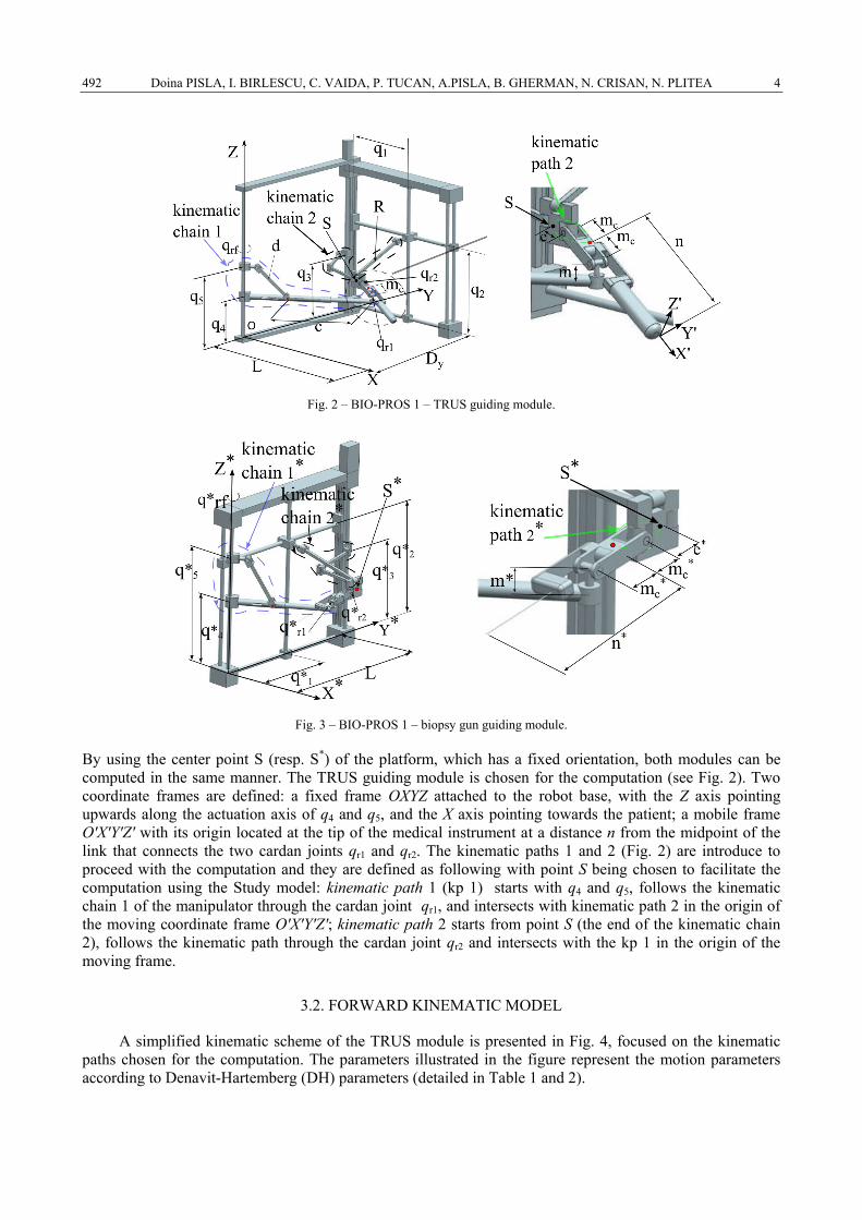
The first module of the robotic system (TRUS probe module), integrates two kinematic chains as illustrated in Fig. 2. The first kinematic chain (kinematic chain 1) is a 3-DOF parallel structure with two actuated joints (q4 and q5) which works in cylindrical coordinates, having the rotation around the common axis of the actuated joints as a free motion. The second kinematic chain (kinematic chain 2) is a 3-DOF parallel structure with three actuated joints (q1, q2 and q3) with constant platform orientation. The two chains are placed in planes that are orthogonal to each other, and they are linked through a pair of Cardan joints. The linkage between the two kinematic chains defines the end effector of the robot which guides the TRUS probe. The second module of the robotic system (Fig. 3 – biopsy gun module), has the same modular structure as the first one, with the difference that both mechanical chains are placed on the same plane of the robot fixed frame. To relate the coordinate frames of the biopsy gun module to the TRUS module one has to use a transformation involving a rotation around O*Z* by π/2 and a translation on O*X* by L.

492 Doina PISLA, I. BIRLESCU, C. VAIDA, P. TUCAN, A.PISLA, B. GHERMAN, N. CRISAN, N. PLITEA 4

Fig. 2 – BIO-PROS 1 – TRUS guiding module.

Fig. 3 – BIO-PROS 1 – biopsy gun guiding module.

By using the center point S (resp. S*) of the platform, which has a fixed orientation, both modules can be computed in the same manner. The TRUS guiding module is chosen for the computation (see Fig. 2). Two coordinate frames are defined: a fixed frame OXYZ attached to the robot base, with the Z axis pointing upwards along the actuation axis of q4 and q5, and the X axis pointing towards the patient; a mobile frame O'X'Y'Z' with its origin located at the tip of the medical instrument at a distance n from the midpoint of the link that connects the two cardan joints qr1 and qr2. The kinematic paths 1 and 2 (Fig. 2) are introduce to proceed with the computation and they are defined as following with point S being chosen to facilitate the computation using the Study model: kinematic path 1 (kp 1) starts with q4 and q5, follows the kinematic chain 1 of the manipulator through the cardan joint qr1, and intersects with kinematic path 2 in the origin of the moving coordinate frame O'X'Y'Z'; kinematic path 2 starts from point S (the end of the kinematic chain 2), follows the kinematic path through the cardan joint qr2 and intersects with the kp 1 in the origin of the moving frame.

3.2. FORWARD KINEMATIC MODEL

A simplified kinematic scheme of the TRUS module is presented in Fig. 4, focused on the kinematic paths chosen for the computation. The parameters illustrated in the figure represent the motion parameters according to Denavit-Hartemberg (DH) parameters (detailed in Table 1 and 2).

5 Algebraic modeling of kinematics and singularities for a prostate biopsy patallel robot 493

Fig. 4 – Kinematic representation for the two kinematic paths.

Table 1

DH parameters for the first kinematic path

DH matrix Mechanical joint Geometric par. Actuation Td = I4 – – Initial displacement, identity matrix

T1 q4 t1 Active translation along Z axis T2 qrf t2 Free rotation around Z axis T3 q4, q5 t3 Active translation along X axis T4 qr1 t4 Free rotation around Z axis T5 qr1 t5 Free rotation around Y axis TM – m Geometric par., translation along Z axis TMC – mc Geometric par., translation along X axis TMn – n Geometric par., translation along X axis

Table 2

DH parameters for the second kinematic path

DH matrix Mechanical joint Geometric par. Actuation S q1, q2, q3 Xm, Ym, Zm Initial displacement SE – e Geometric par., translation along X axis S2 qr2 s2 Free rotation around Z axis S3 qr2 s3 Free rotation around Y axis

SMC – mc Geometric par., translation along X axis SMn – n Geometric par., translation along X axis

Using DH parameters, the constraint equations are defined in Eq. (8)–(9), where the left hand side

represent the kinematic constrains in matrix form (note that the matrices are in the form of Eq. 1), and the right hand side are the DH parameters matrices (described in Table 1 for the kinematic path 1, and Table 2 for the kinematic path 2). For the computation, the robot pose was chosen in a convenient way to write the DH parameter in a simple manner. The free rotation parameters s2, s3, and t2, t4, t5 are derived from rotation matrices, with the trigonometric functions (sines and cosines naturally found in the rotation matrices) written in parametric form using the tangent of half angle formulas cos(θ) = (1–t2

i)/(1+t2i), sin(θ) = 2t2

i/(1+t2i) for the

first kinematic path and cos(θ)=(1–s2i)/(1+s2

i), sin(θ) = 2s2i/(1+s2

i) for the second kinematic path, where θ is the angle of rotation in the rotation matrices. The point S (Xm; Ym; Zm) and the values for t1 and t3 (i.e. the active joint parameters) are derived from the relations presented in Eq. (10) (Fig. 2) [7].

1 1 2 3 4 5d M MC MnK T T T T T T T T T= ⋅ ⋅ ⋅ ⋅ ⋅ ⋅ ⋅ ⋅ (8)

2 2 3E MC MnK S S S S S S= ⋅ ⋅ ⋅ ⋅ ⋅ (9)

1mX q= ; 2 23 2( )m yY D R q q= − − − ; 3mZ q= ; 1 4t q= ; 2 2

3 4 5( )t c d q q= + − − . (10)

Following the constraint equations (Eq. 8–9) and the Study model described in Eq. (6)–(7), the Study parameters are computed for the two kinematic chains yielding:

494 Doina PISLA, I. BIRLESCU, C. VAIDA, P. TUCAN, A.PISLA, B. GHERMAN, N. CRISAN, N. PLITEA 6

0 2 4

1 2 4 5

2 2 4 5

3 2 4

2 2 2 3 4 4 3 4 5 2 1 2 1 4 40

1 2 4 2 4 1 5 2 4 2 4 2 3 4 31

1 2 2 4 1 42

3

2 22( )

2( 1 )2( )

( )( )( )

c c

c c

x t tx t t tx t t tx t t

m t nt t t nt m t t t t mt t t t t mtyt t t mt t t m t nt t m t t t t t m t nyt t mt mt t ty

y

− − + − − +

− + = − + − + − − − − −

− + + − + + − + + + + +

5 2 2 3 2 3 4 4 4

2 4 2 4 2 3 4 3 5 1 2 4 2 4 1( )c c

c c

t m t t t nt t t m t ntnt t m t t t t t n m t t t t t mt t t m

− + + − − + − + − + − − − − + +

(11)

0

1 2 3

2 3

3 2

2 3 2 3 2 3 2 3 3 20

3 21

2 3 2 2 2 22

2 3 3 3 3 33

22

22

c m m m

m m m c

m m c m

m m c m

xx s sx sx s

m s s ns s es s X s s Y s Z syZ s Y s X e n my

Z s s X s ns es m s YyY s s es X s m s ns Zy

− = + + + − +

− − − − − − + ⋅ − + − −

+ + − − −

(12)

Two ideals of varieties are generated: I generated by the 8 equations within Eq. 11 representing the polynomial ideal of the kinematic constraints of the kinematic path 1; I ‘generated by the 8 equations within Eq. 12 representing the polynomial ideal for kinematic path 2. With the ideal representation two lexdeg (monomial ordering to eliminate variables when an entire lexicographic base is not needed) Groebner basis were computed for the ideals (G for I, and G’ for I ‘) by eliminating all the free rotation parameters (considered unknowns) therefore depending only on the structural parameters of the robot and the values for the robot active joints. The computed bases contain 9 equations (all of them of degree 2) for I, and 5 equations (4 of degree 1 and 1 of degree 2) for I ‘, the unknowns being the Study parameters. Due to the length of the equations of the computed bases only the first 4 equations from G’ are shown (Eq. 13).

2 2 2 2 23 0 1 2

2 2 2 2 22 0 1 3

2 2 2 2 21 0 2 3

2 2 2 2 20

' ( 2 ) 2 2 2( ) ;

( 2 ) 2 2 (2 2 2 ) ;

( 2 ) 2( ) 2 2 ;

( 2 ) 2(

m m m m c m m m c

m m m m c m m m c

m m m m c m c m m

m m m m c

G Y Z eX e X m x Z y Y y X e m y

Y Z eX e X m x Y y Z y e X m y

Y Z eX e X m x X e m y Z y Y y

Y Z eX e X m x e

=< + + + + − − + + − − −

+ + + + − ⋅ − ⋅ − + + +

+ + + + − + − − + + −

+ + + + − + 1 2 3) 2 2 ;...m c m mX m y Y y Z y+ − + + >

(13)

To solve the forward kinematic problem using the Study model, first, a pure lexicographic Groebner basis ( G ) is computed from the reunion of the two bases (G and G’) and by adding the normalizing condition (x2

0+x21+x2

2+x23=1), followed by adding the numerical values for the active joint parameters (for both bases

G and G’). Maple software was able to compute the basis G after the numerical values for structural parameters were given {e=70; m=50; mc=75; n=270} (dimensions considered in mm). An example is illustrated with the numerical values for active joint parameters being {Xm=250; Ym=200; Zm= 110, t1=100; t3=350}. After the substitution the basis G contains a univariate polynomial in x3 of degree 8. Solving the basis yields 8 solutions for the Study parameters 4 of them being presented in Table 3 (the 4 other solutions are the presented one multiplied by –1).

7 Algebraic modeling of kinematics and singularities for a prostate biopsy patallel robot 495

Table 3

Numerical values for the Study parameters

x0 x1 x2 x3 y0 y1 y2 y3 –0.127 0.306 0.942 0.042 157.054 72.936 1.036 –77.745 0.086 0.759 –0.637 0.103 91.977 –62.399 –37.777 149.167

–0.759 0.086 0.103 0.637 62.399 91.976 149.166 37.777 0.306 0.127 –0.042 0.942 72.937 –157.054 77.745 1.037

From the numerical solutions of the Study parameters the Euclidean displacement may be computed with a top perspective of the mechanism illustrated in Fig. 5. Two forward kinematics are of interest, the other two being a rotated version of the first two (by a value of π around the Z’ axis and the Y’ axis).

3.3. SINGULARITIES

A singularity of a robot may occur when two or more solutions for the forward kinematics coincide. The Groebner basis G computed with numerical values for the structural parameters (described in section 3.1) contains an univariate polynomial in x3. For two or more solutions to coincide the discriminant of the univariate polynomial (computed by taking its resultant with its first derivative in x3) must vanish. Maple software returned a factorised discriminant with 8 factors representing the singularity conditions. Five factors are presented in Eq. (14)–(18), while the last 3 since they are too long are presented in their general form. The degree of Eq. (19)–(20) is 4, while the degree of Eq. (21) is 8.

0mY = (14)

1 100 0mZ t− + = (15)

1 200 0mZ t− − = (16)

150 0mZ t− − = (17)

2 2140 4900 0m m mX X Y+ + + = (18)

1 1 3( , , , , ) 0sig m m mf X Y Z t t = (19)

2 1 3( , , , , ) 0sig m m mf X Y Z t t = (20)

3 1 3( , , , , ) 0sig m m mf X Y Z t t = (21)

Fig. 5 – Kinematic solutions using Study parameters.

Equation (14) defines the first singularity when the end effector lies in the XOZ plane of the robot coordinate system. This singularity is easy to observe (see Fig. 4 – the computation was started in this pose) but it's physically impossible for the robot to reach that position due to mechanical constraints. Eq. (15)–(16) defines the second singularity with the end effector positioned vertically. These singularities are avoided in the robot control (or in the mechanical design of the Cardan joints). A kinematic representation for these two singularities is presented in Fig. 6.

496 Doina PISLA, I. BIRLESCU, C. VAIDA, P. TUCAN, A.PISLA, B. GHERMAN, N. CRISAN, N. PLITEA 8

Fig. 6 – Second singularity poses. Fig. 7 – Third singular pose.

Equation (17) describes the third singularity when the end effector lies in a horizontal plane. Figure 7 shows one singular representation that satisfies the condition, when the circle generated by the centre of qr2 with radius 2 cm⋅ , and the circle generated from Z axis with radius t3 are tangent. Equation (18) does not have real solution so it is not of interest.

The final three factors (Eq. 19–21), were evaluated using fixed values {t1 = 200; t3 = 350}, and letting Xm, Ym, Zm to vary in the intervals: [ ] [ ] [ ]X 0,500 ,Y 0,500 ,Z 0,500 .m m m∈ ∈ ∈

Fig. 8 – Singular pose and surface described by Eq. (19). Fig. 9 – Singular pose and surface described by Eq. (20).

The implicit surfaces are illustrated in Fig. 8 and 9 (along with CAD representations for the singular pose), for Eq. (19)–(20). The only real solutions found for Eq. (21) were found when it was evaluated with Zm = 250. This result implies that Eq. (21) is redundant with Eq. (17) (since 250 = t1 + 50). Figure 8 illustrates a singular pose where the end effector has the same orientation as the platform with constant orientation and points towards the YOZ plane – which is physically impossible). Figure 9 illustrates a singular pose where the end effector is along the kinematic chain 1 which should be avoided in the robot control algorithm). The singularity conditions computed with the Study parameters model are in active joint space, and can be easily implemented in the robot control (by relating the active joint parameters with Eq. 10 – where the active joints are read from the position sensors) as safety condition in the real time control (in a cyclic closed loop control system). Furthermore, the singularities were computed for the mechanism that drives the platform with constant orientation, since the computation so far was based on introducing a point (S) at the start of the kinematic path 2. A path was defined starting from q1 and q2, following the kinematic path through R (path a in Fig. 10a) and ending in S; a second path was introduced starting from q3, following the kinematic path through K1 and ending in S (path b in Fig. 9a). The resulted equations are presented below with Eq. (22) describing the platform with constant orientation in the plane XOY. Eq. (23)–(24) describes a singularity where the link R is in a vertical position (the kinematic link 1 cannot reach that position due to mechanical constraints) as illustrated in Fig. 10b.

9 Algebraic modeling of kinematics and singularities for a prostate biopsy patallel robot 497

0yD = (22) 032 =−+− qqR (23) 032 =−+ qqR (24)

Fig. 10 – a) Kinematic paths for the platform with constant orientation; b) singularity poses.

4. CONCLUSIONS

Using Study parametrization and methods of computing polynomial equations, the mathematical model for the forward kinematics and singularities of BIO-PROS 1 was achieved. Despite the complexity of the parallel robot, Maple was able to compute the mathematical models after a simplification was made, by introducing a point (S) which serves as: a mid-point for the computation (eliminates the memory failure of Maple when it processes large equations); and a point to generalize the computation, so it can be used for both TRUS module and biopsy gun module. Having a parametric description of the kinematic model enables the bridging between the theoretical model and the robotic prototype by implementing the singularities polynomials as real time safety condition in the robot controller.

REFERENCES

1. SIEGEL R., MILLER K, Cancer statistics. CA Cancer J Clin., 65, pp. 5–29, 2015. 2. FERLAY J., STELIAROVA-FOUCHER E., Cancer statistics. CA Cancer J Clin., 65, pp. 5–29, 2015. 3. VAIDA C. et al., Design of a Needle Insertion Module for Robotic Assisted Transperineal Prostate Biopsy, New Trends in

Medical and Service Robots. Mechanisms and Machine Science, Springer, 48, 2018. 4. CHANG D., CHALLACOMBE B., LAWRENTSCHUK N., Transperineal biopsy of the prostate-is this the future?, Nature

Reviews Urology, 2013. 5. TARUN K. P. et al., AAPM and GEC-ESTRO guidelines for image-guided robotic brachytherapy, Report of Task Group 192.

Am. Assoc. Phys. Med., 2014. 6. PLITEA N. et al., Family of innovative parallel robots for transperineal prostate biopsy, Patent pending: A/00191/13.03.2015 7. PISLA D. et al., On the Kinematics of an Innovative Parallel Robotic System for Transperineal Prostate Biopsy, 14th World

Congress in Mechanism and Machine Science, Taipei (Taiwan), 25–30 October, 2015. 8. HUSTY M., PFURNER M., SCHROECKER H.P., Algebraic Methods in Mechanism Analysis and Synthesis, Robotica, 25, 6,

pp. 661–675, 2007. 9. HUSTY M., SCHROECKER H.P., Algebraic Geometry and Kinematics, Nonlinear Computational Geometry, 151,

pp. 85–107, October 2009. 10. ANGELES J., Fundamentals of Robotic Mechanical Systems, Theory, Methods and Algorithms, Springer, New York, 1997. 11. BERCEANU, C., TARNITA, D., FILIP, D., About an experimental approach used to determine the kinematics of the human

finger, Journal of the Solid State Phenomena, Robotics and Automation Systems, 166–167, pp. 45–50, 2010. 12. TARNITA, D., Wearable sensors used for human gait analysis, Romanian Journal of Morphology and Embryology, 57, 2,

pp. 373–382, 2016. 13. SCHADLBAUER J., WALTER D.R., HUSTY M., The 3-RPS parallel manipulator from an algebraic viewpoint, Mechanism

and Machine Theory, 75, pp. 161–176, 2014. 14. VAIDA C. et al., Kinematic Analysis of an Innovative Medical Parallel Robot Using Study Parameters, New Trends in

Medical and Service Robots. Mechanisms and Machine Science, Springer, 39, pp. 85–99, 2016. 15. SCHADLBAUER J. et al., A Complete Analysis of Singularities of a Parallel Medical Robot, Advances in Robot Kinematics

2016. Springer Proceedings in Advanced Robotics, 4. Springer, pp. 81–89, 2018.

Received December 29, 2017

a) b)