Algebraic Systems Theory - Lehrstuhl D für MathematikEva.Zerz/ast.pdf · Algebraic Systems Theory...

Algebraic Systems Theory

Eva ZerzLehrstuhl D fur Mathematik

RWTH Aachen

Februar 2006

Contents

1 Introduction 5

2 Abstract linear systems theory 9

2.1 Galois correspondences . . . . . . . . . . . . . . . . . . . . . . . . 10

2.2 Property O . . . . . . . . . . . . . . . . . . . . . . . . . . . . . . 14

2.3 The Malgrange isomorphism . . . . . . . . . . . . . . . . . . . . . 18

2.4 Injective cogenerators . . . . . . . . . . . . . . . . . . . . . . . . . 20

3 Basic systems theoretic properties 25

3.1 Autonomy . . . . . . . . . . . . . . . . . . . . . . . . . . . . . . . 25

3.2 Input-output structures . . . . . . . . . . . . . . . . . . . . . . . . 30

3.3 Controllability . . . . . . . . . . . . . . . . . . . . . . . . . . . . . 31

3.4 The controllable part of a system . . . . . . . . . . . . . . . . . . 34

3.5 Observability . . . . . . . . . . . . . . . . . . . . . . . . . . . . . 37

4 One-dimensional systems 39

4.1 Ordinary differential equations . . . . . . . . . . . . . . . . . . . . 39

4.2 Rationally time-varying systems . . . . . . . . . . . . . . . . . . . 42

4.3 Time-invariant case . . . . . . . . . . . . . . . . . . . . . . . . . . 50

5 Multi-dimensional systems 51

5.1 Interpretation of autonomy and controllability . . . . . . . . . . . 51

3

4 CONTENTS

5.2 The dimension of a system . . . . . . . . . . . . . . . . . . . . . . 56

5.3 Autonomy degrees . . . . . . . . . . . . . . . . . . . . . . . . . . 59

5.4 Free systems . . . . . . . . . . . . . . . . . . . . . . . . . . . . . . 63

A Background material 69

A.1 Kalman controllability criterion . . . . . . . . . . . . . . . . . . . 69

A.2 Galois correspondences . . . . . . . . . . . . . . . . . . . . . . . . 74

A.3 Property O for 1-d time-invariant systems . . . . . . . . . . . . . 77

A.4 Left-exactness of the Hom-functor . . . . . . . . . . . . . . . . . . 79

A.5 Baer’s criterion . . . . . . . . . . . . . . . . . . . . . . . . . . . . 80

A.6 Criterion for the cogenerator property . . . . . . . . . . . . . . . . 83

A.7 Injective cogenerator property for 1-d time-invariant systems . . . 86

A.8 Ore domains and fields of fractions . . . . . . . . . . . . . . . . . 87

A.9 Linear algebra over skew fields . . . . . . . . . . . . . . . . . . . . 89

A.10 Controllability and observability . . . . . . . . . . . . . . . . . . . 92

A.11 Jacobson form . . . . . . . . . . . . . . . . . . . . . . . . . . . . . 96

A.12 The tensor product . . . . . . . . . . . . . . . . . . . . . . . . . . 100

Chapter 1

Introduction

Classical linear systems theory studies, e.g., the continuous and discrete models

(C) x(t) = Ax(t) +Bu(t)(D) x(t+ 1) = Ax(t) +Bu(t)

where A ∈ Rn×n and B ∈ Rn×m. One calls

x : T → Rn and u : T → R

m

the state function and the input function, respectively. The set T representsa mathematical model of time, e.g., T = R or T = [0,∞) in the continuouscase (C), and T = Z or T = N in the discrete case (D).

For (C), we additionally require that u ∈ U, where U is a function space thatguarantees the solvability of (C), that is,

∀u ∈ U ∃x : x = Ax+Bu.

For example, this is true whenever U ⊆ C0(R,Rm), the set of continuous functionsfrom T = R to Rm. We will make this assumption for the rest of this chapter.Note that no such condition is needed for (D), which is always recursively solvable,at least for all t ≥ t0 if x(t0) is given. To unify the notation, we put U = (Rm)T

for (D), which is the space of all functions from T to Rm.

Solving (C) and (D) is not a problem (up to numerical issues), because, imposingthe initial condition x(t0) = x0, we have the solution formulas

(C) x(t) = eA(t−t0)x0 +∫ tt0eA(t−τ)Bu(τ)dτ

(D) x(t) = At−t0x0 +∑t−1

τ=t0At−1−τBu(τ) for t ≥ t0.

The goal of control theory is not to solve (C) and (D) for a given input function,but rather, to design an input function such that the solution has certain desired

5

6 CHAPTER 1. INTRODUCTION

properties. For this, one needs to study the structural properties of the underlyingsystem.

One of the most important issues in control theory is the question of controlla-bility: Given x0, x1 ∈ Rn and t0, t1 ∈ T with t0 < t1, does there exist u ∈ U suchthat the solution to (C) or (D) with x(t0) = x0 satisfies x(t1) = x1? If yes, wesay that x0 can be controlled to x1 in time t1 − t0 > 0.

Interpretation: One should think of t0 and x0 as a given initial time and state,whereas t1 and x1 represents a desired terminal time and state. The problem isto find an input function u such that the system goes to state x1 in finite timet1 − t0 > 0, when started in state x0 at time t0. Without loss of generality, weput t0 = 0 from now on. Then t1 > 0 is the length of the transition period fromthe initial state x(0) = x0 to the terminal state x(t1) = x1.

Theorem 1.1 The following are equivalent:

1. There exists 0 < t1 ∈ T such that any x0 ∈ Rn can be controlled to anyx1 ∈ Rn in time t1.

2. rank[B,AB, . . . , An−1B] = n.

Proof: We do this only for the discrete case (D), where it is elementary. Fromx(t+ 1) = Ax(t) +Bu(t) and x(0) = x0, we get recursively

x(t1) = At1x0 +

t1−1∑τ=0

At1−τ−1Bu(τ).

Thus the requirement that x(t1) = x1 is equivalent to

x1 = At1x0 +Kt1v

where

Kt1 = [B,AB, . . . , At1−1B] and v =

u(t1 − 1)...

u(0)

.The equation Kt1v = x1 − At1x0 has a solution v for any choice of x0, x1 if andonly if Kt1 has full row rank, that is, rank(Kt1) = n. However, the existence of t1with rank(Kt1) = n is equivalent to rank(Kn) = n. This is quite clear for t1 < n,and for all t1 ≥ n, we have

rank[B,AB, . . . , At1−1B] = rank[B,AB, . . . , An−1B].

7

This follows from considering the sequence

0 ⊆ im(B) ⊆ im[B,AB] ⊆ . . . ⊆ im[B,AB, . . . , An−1B]?

⊆ . . . ⊆ Rn

of subspaces of Rn, which must become stationary. Considering the dimensionsof these spaces, one can see that this cannot happen later than at the inclusionmarked by a star.

If assertion 1 from the theorem is true, we say that the system is controllable.The matrix K = Kn = [B,AB, . . . , An−1B] is called Kalman controllabil-ity matrix and Theorem 1.1 is sometimes referred to as Kalman controllabilitycriterion.

What can we say about (C)? Let us first give a careful restatement of the theorem.

Theorem 1.2 (Theorem 1.1 restated for (C)) The following are equivalent:

1. ∃t1 > 0 ∀x0, x1 ∈ Rn ∃u ∈ U such that the solution to

x = Ax+Bu, x(0) = x0

satisfies x(t1) = x1.

2. rank[B,AB, . . . , An−1B] = n.

Note that assertion 1 describes an analytic property of the system, whereas as-sertion 2 is a purely algebraic condition. An immediate question concerns therole of the set U which does not appear in assertion 2. For which sets U is thetheorem valid? It turns out that the theorem holds for a wide range of inputfunction spaces, more precisely, for any U with

U ⊇ O(R,Rm),

where O denotes the analytic functions. Since this condition is met by a lot ofrelevant function spaces U, we can say that the theorem is relatively independentof the specific signal space. This contributes to its importance and applicability.It is a prominent example of an algebraic characterization of a systems theoreticproperty, which is at the heart of algebraic systems theory.

Roughly speaking, the goals of algebraic systems theory are:

• translating analytic properties of systems to algebraic properties and viceversa;

• characterizing the signal spaces for which this is possible.

8 CHAPTER 1. INTRODUCTION

Chapter 2

Abstract linear systems theory

Let D be a ring (with unity), let A be a left D-module, and let q be a positiveinteger. An abstract linear system has the form

B := w ∈ Aq | Rw = 0,where R ∈ Dg×q for some positive integer g.

Interpretation: One should think of A as the signal set. Our system involves qsignals, that is, we have signal vectors in Aq. The set B tells us which w ∈ Aqcan occur in the system: namely, those which satisfy the system law Rw = 0.This is a linear system of equations, where the entries of R are elements of D.The ring D should be thought of as a ring of operators acting on A. Since A is aleft D-module, the expression Rw is a well-defined element of Ag. One calls R arepresentation of B, because in general, there are many different R’s that lead tothe same B, whereas B is uniquely determined by R (once A is fixed). If R has grows, then g is the number of defining equations in the given representation Rof B. Note that in contrast to q, the number g is not an intrinsic system property(for instance, there may be superfluous equations in the chosen representation R).The letter B comes from the word “behavior” which was introduced by J. C.Willems [20, 24].

Examples: Let K denote either R or C.

• Let D = K[ ddt

]. This leads to the class of systems given by linear ordinarydifferential equations with constant coefficients. Signal sets A with a D-module structure are, e.g., A = C∞(R,K), the space of smooth functions,or D′(R,K), the space of distributions etc. For example, the system x =Ax+Bu could be written as an abstract linear system by putting

w =

[xu

]and R =

[ddtI − A, −B

].

9

10 CHAPTER 2. ABSTRACT LINEAR SYSTEMS THEORY

• Let D = F[σ], where F is a field, and σ is the shift operator defined by(σa)(t) = a(t + 1) for all a ∈ A. This leads to the class of systems givenby linear ordinary difference equations with constant coefficients. Suitablesignal sets areA = FT , where T = N or T = Z. For x(t+1) = Ax(t)+Bu(t),one sets

w =

[xu

]and R =

[σI − A, −B

].

• Let D = K[ ddt, σ]. This leads to the class of linear delay-differential systems

with constant coefficients. A signal set is given by A = C∞(R,K).

• Let D = K〈t, ddt〉. This leads to the class of systems given by linear or-

dinary differential equations with polynomial coefficients. The signal setsconsidered in the first example are still suited. The ring D is known asWeyl algebra. In contrast to the other examples, it is non-commutative,because

ddtta = a+ t d

dta for all a ∈ A

and thus ddtt−t d

dt= 1. Another non-commutative case is given byD = K[ d

dt]

where K is a field of functions, e.g., K = K(t), the field of rational functions,orK =M, the field of meromorphic functions. This leads to linear ordinarydifferential equations with coefficients in K. We have d

dtk − k d

dt= k′. A

signal set is given by A = K.

• Let D = F〈t, σ〉. This leads to the class of linear ordinary difference equa-tions with polynomial coefficients. The signals sets A = FT still work.

• Let D = K[∂1, . . . , ∂n]. This leads to the class of systems given by linearpartial differential equations with constant coefficients. As signal sets, onecould take A = C∞(Rn,K) or A = D′(Rn,K).

• Finally, D = F[σ1, . . . , σn] leads to the class of linear partial differenceequations with constant coefficients. A signal set is A = FT

n, the set of all

n-fold indexed sequences with values in F. ♦

2.1 Galois correspondences

Let B ⊆ Aq. Define

M(B) := m ∈ D1×q | mw = 0 for all w ∈ B.

Lemma 2.1 M(B) is a left D-submodule of D1×q.

2.1. GALOIS CORRESPONDENCES 11

Proof: Let m1,m2 ∈ M(B), d1, d2 ∈ D. Since m1w = m2w = 0 for all w ∈ B,we have (d1m1 + d2m2)w = 0 for all w ∈ B. Thus d1m1 + d2m2 ∈M(B).

We call M(B) the module of all equations satisfied by B. Conversely, letM ⊆ D1×q. Define

B(M) := w ∈ Aq | mw = 0 for all m ∈M.

Lemma 2.2 B(M) is an (additive) Abelian subgroup of Aq.

Proof: We have 0 ∈ B(M) and if w,w1, w2 ∈ B(M), then −w ∈ B(M) andw1 + w2 ∈ B(M).

Note: B(M) is not a left D-submodule of Aq, in general.

Example: Let D = K〈t, ddt〉, A = K[t], and q = 1. Take M = d

dt, then

B(M) = w ∈ A | dwdt

= 0,which clearly consists of all constants. Hence for any 0 6= c ∈ K, we havec ∈ B(M), but tc /∈ B(M), showing that B(M) is not a left D-module. ♦

Remark: If D is commutative, then B(M) is a (left) D-module. To see this, letw1, w2 ∈ B(M) and d1, d2 ∈ D. Since mw1 = mw2 = 0 for all m ∈ M , we havem(d1w1 + d2w2) = md1w1 + md2w2 = d1mw1 + d2mw2 = 0 for all m ∈ M andhence d1w1 + d2w2 ∈ B(M).

Let A denote the set of all Abelian subgroups of Aq and let M denote the set ofall left D-submodules of D1×q. We have a Galois correspondence

A ↔ M

B → M(B)

B(M) ← M.

The term “Galois correspondence” means that

• M and B are inclusion-reversing, that is,

B1 ⊆ B2 ⇒M(B1) ⊇M(B2) and M1 ⊆M2 ⇒ B(M1) ⊇ B(M2);

• B ⊆ BM(B) for all B and M ⊆MB(M) for all M .

Lemma 2.3 Let B1, B2 ∈ A and M1,M2 ∈M. Then we have

B(M1 +M2) = B(M1) ∩B(M2) (2.1)

M(B1 ∩B2) ⊇ M(B1) + M(B2) (2.2)

B(M1 ∩M2) ⊇ B(M1) + B(M2) (2.3)

M(B1 +B2) = M(B1) ∩M(B2). (2.4)


Moreover, B(0) = Aq, B(D1×q) = 0, M(0) = D1×q.

Proof: Let w ∈ B(M1 +M2). This means that (m1 +m2)w = 0 for all m1 ∈M1,m2 ∈ M2. Since 0 ∈ Mi, this is equivalent to m1w = 0 and m2w = 0 for allm1 ∈M1 and all m2 ∈M2. Thus, still equivalently, w ∈ B(M1) ∩B(M2).

Let m ∈M(B1) + M(B2), that is, m = m1 +m2 with m1w1 = 0 for all w1 ∈ B1

and m2w2 = 0 for all w2 ∈ B2. Let w ∈ B1 ∩ B2, then mw = m1w + m2w = 0.Thus m ∈M(B1 ∩B2).

Let w ∈ B(M1) + B(M2), that is, w = w1 + w2 with m1w1 = 0 for all m1 ∈ M1

and m2w2 = 0 for all m2 ∈M2. Let m ∈M1 ∩M2. Then mw = mw1 +mw2 = 0.Thus w ∈ B(M1 ∩M2).

Let m ∈M(B1 +B2). This means that m(w1 +w2) = 0 for all w1 ∈ B1 , w2 ∈ B2.Since 0 ∈ Bi, this is equivalent to mw1 = 0 for all w1 ∈ B1 and mw2 = 0 for allw2 ∈ B2. Still equivalently, m ∈M(B1) ∩M(B2).

Remark: Note that the three equalities B(0) = Aq, B(D1×q) = 0, M(0) = D1×q

are more or less trivial, whereas M(Aq) = 0 is not true in general.

Assumption: Let us assume from now on that D is left Noetherian. This meansthat the following equivalent conditions are satisfied:

• Every ascending chain I0 ⊆ I1 ⊆ I2 ⊆ . . . of left ideals in D must becomestationary.

• Every left ideal I in D is finitely generated.

• Every non-empty set of left ideals in D possesses a maximal element (withrespect to inclusion).

Note that in all of the examples from above, D is left Noetherian (if D is com-mutative, there is no need to distinguish between left and right Noetherian, andthen one simply says “Noetherian”). If D is left Noetherian, then the finitelygenerated D-module D1×q is a left Noetherian module, which means that thefollowing equivalent conditions are satisfied:

• Every ascending chain M0 ⊆ M1 ⊆ M2 ⊆ . . . of left submodules of D1×q

must become stationary.

• Every left submodule of D1×q is finitely generated.

• Every non-empty family of left submodules of D1×q possesses a maximalelement.

2.1. GALOIS CORRESPONDENCES 13

Thus every M ∈M is finitely generated, that is, M = D1×gR for some suitableinteger g and R ∈ Dg×q. Then

B(M) = w ∈ Aq | Rw = 0.

Hence we can characterize B := B(M) as follows: It consists of all B of the formB = w ∈ Aq | Rw = 0, where R is an arbitrary D-matrix with q columns, thatis, B consists of all abstract linear systems.

Thus we have an induced Galois correspondence

B ↔ M (2.5)

B → M(B)

B(M) ← M

withBM(B) = B

for all abstract linear systems B ∈ B. On the other hand, we only have

MB(M) ⊇M

for M ∈ M. The module MB(M) is sometimes called the (Willems) closureof M with respect to A, denoted by M := MB(M). This is due to the followingproperties, which hold for all M,M1,M2 ∈M:

• M ⊆M ;

• M = M ;

• M1 ⊆M2 ⇒M1 ⊆M2.

The module M is called (Willems) closed with respect to A if M = M , orequivalently, if M ∈ im(M).

Using these notions, we can be more specific about the inclusion (2.2).

Lemma 2.4 Let B1,B2 ∈ B. Then

M(B1 ∩ B2) = M(B1) + M(B2).

Proof: We have Bi = BM(Bi) and thus

M(B1 ∩ B2) = M(BM(B1) ∩BM(B2))

= MB(M(B1) + M(B2))

= M(B1) + M(B2),


where we have used (2.1).

In what follows, we will study D-modules A with the property that every M ∈Mis closed with respect to A. This is equivalent to M = im(M). Then the Galoiscorrespondence (2.5) will become a pair of inclusion-reversing bijections inverseto each other, and the inclusion (2.2) will become an identity when applied toB1,B2 ∈ B. Similarly, we will have M(Aq) = 0. This is a good starting pointfor algebraic systems theory, because it makes it possible to translate statementsfrom the system universe B to the algebraic setting M and vice versa. It will turnout that this works for many relevant choices of D-modules A. A counterexampleis given next.

Example: Let D = K[ ddt, σ] and let A = C∞(R,K). Let R = d

dtand M = DR.

Then B = B(M) consists of all constants functions. However, any constantfunction a also satisfies

a(t+ 1) = a(t) for all t ∈ R.

Thus σ − 1 ∈ M(B) = M , although σ − 1 /∈ M . This shows that the inclusionM ⊂M is strict, in general. ♦

Remark: Note that for M1,M2 ∈M, we have M1∩M2,M1+M2 ∈M. Similarly,forB1, B2 ∈ A, we haveB1∩B2, B1+B2 ∈ A. This was tacitly used in Lemma 2.3.However, B1,B2 ∈ B implies that B1∩B2 ∈ B, but B1 +B2 ∈ B is not necessarilytrue. It turns out that, assuming M = im(M), equality holds in (2.3) if and onlyif B is closed under addition. If we have this additional property, then the Galoiscorrespondence (2.5) will become a lattice anti-isomorphism. This situation isthe optimal environment for algebraic systems theory. Therefore we will alsoinvestigate the question under which conditions B is closed under addition.

2.2 Property O

Let D be a left Noetherian ring, let q be a positive integer, and let M denote theset of all left D-submodules of D1×q. If A is a left D-module, we use the notation

BA(M) := w ∈ Aq | mw = 0 for all m ∈M

for M ∈M and

M(B) := m ∈ D1×q | mw = 0 for all w ∈ B

for B ⊆ Aq. Recall that MA

:= MBA(M) is the closure of M with respect to A.We are interested in D-modules A with the property that every M ∈M is closedwith respect to A. Let us call this property O (named after U. Oberst [17]).

2.2. PROPERTY O 15

Lemma 2.5 Let A1 ⊆ A2 be two left D-modules. If A1 has property O, then sohas A2.

Proof: Let M ∈ M. Since A1 ⊆ A2, we have BA1(M) ⊆ BA2(M). Applyingthe inclusion-reversing map M, we obtain

MA1

= MBA1(M) ⊇MBA2(M) = MA2.

If A1 has property O, then this implies

M = MA1 ⊇M

A2.

Since the inclusion MA2 ⊇M is always true, we obtain M = M

A2. Thus A2 has

property O.

Some signal sets with property O

Theorem 2.6 Let D = K[ ddt

]. Let A be the set of all polynomial-exponentialfunctions, that is, all a of the form

a(t) =∑k

i=1 pi(t)eλit for all t ∈ T = R

where k ∈ N, pi ∈ C[t] and λi ∈ C. Then A has property O.

Remark: If K = R, one has to make the additional assumption that for all i withpi 6= 0, there exists j such that λj = λi and pj = pi in order to get real-valuedsignals. In the following, this will be taken for granted tacitly.

Thus all K[ ddt

]-modules that contain the polynomial-exponential functions alsohave property O. This is true for O(R,K), C∞(R,K), and even D′(R,K) (usingthe usual identification between a continuous function and the regular distributionit generates).

The discrete counterpart of the above theorem is stated next.

Theorem 2.7 Let D = K[σ]. Let A be the set of all polynomial-exponentialfunctions, that is, all a of the form

a(t) =∑k

i=1 pi(t)λit for all l ≤ t ∈ T = N

where k, l ∈ N, pi ∈ C[t] and λi ∈ C. Then A has property O.


Remark: Thus the K[σ]-module KN has property O. Note that Theorem 2.7 isnot valid for T = Z. This can be seen from the following example. However, theproblem can easily be repaired, see Theorem 2.8 below.

Example: Let R = σ and M = K[σ]R. Since σ is invertible on KZ, we obtain

BA(M) = 0 for A = KZ. Thus M

A= K[σ] 6= M . This shows that no A ⊆ KZ

has property O as a K[σ]-module. ♦

Theorem 2.8 Let D = K[σ, σ−1]. Let A be the set of all polynomial-exponentialfunctions, that is, all a of the form

a(t) =∑k

i=1 pi(t)λit for all t ∈ T = Z

where k ∈ N, pi ∈ C[t] and λi ∈ C \ 0. Then A has property O.

Remark: Thus KZ has property O when considered as a module over the ringD = K[σ, σ−1].

Theorem 2.9 Let n be a positive integer and let D = K[∂1, . . . , ∂n]. Let A bethe set of all polynomial-exponential functions, that is, all a of the form

a(t) =∑k

i=1 pi(t)eλit for all t ∈ Rn

where k ∈ N, pi ∈ C[t1, . . . , tn] and λi ∈ C1×n. Then A has property O.

Remark: Therefore, allK[∂1, . . . , ∂n]-modules that contain the polynomial-expo-nential functions also have property O. This is true, e.g., forO(Rn,K), C∞(Rn,K),and D′(Rn,K).

Also this theorem has discrete counterparts.

Theorem 2.10 Let D = K[σ1, . . . , σn]. Let A be the set of all polynomial-exponential functions, that is, all a of the form

a(t) =∑k

i=1 pi(t)λti for all l ≤ t ∈ Nn

where k ∈ N, l ∈ Nn (l ≤ t means li ≤ ti for all i) pi ∈ C[t1, . . . , tn] andλi ∈ C1×n. Here, λti = λt1i1 · · ·λ

tnin has to be understood as a multi-index notation.

Then A has property O.

Theorem 2.11 Let D = K[σ1, . . . , σn, σ−11 , . . . , σ−1

n ]. Let A be the set of allpolynomial-exponential functions, that is, all a of the form

a(t) =∑k

i=1 pi(t)λti for all t ∈ Zn

where k ∈ N, pi ∈ C[t1, . . . , tn] and λi ∈ (C \ 0)1×n. Then A has property O.

Remark: Thus the K[σ1, . . . , σn]-module A = KNn

has property O, and the sameholds for the K[σ1, . . . , σn, σ

−11 , . . . , σ−1

n ]-module A = KZn.

2.2. PROPERTY O 17

Consequences of property O

Let A be a D-module with property O. Then the Galois correspondence

B ↔ M

B → M(B)

B(M) ← M

consists of two inclusion-reversing bijections inverse to each other. Concretely,we have a 1-1 correspondence between B = w ∈ Aq | Rw = 0 and M = D1×gRfor any R ∈ Dg×q. In particular, we have M(Aq) = 0, that is, there is non-zerom ∈ D1×q such that m annihilates all signal vectors w ∈ Aq, or equivalently,there is no 0 6= d ∈ D such that dA = 0.

Moreover, we have for all B1,B2 ∈ B and all M1,M2 ∈M

B(M1 +M2) = B(M1) ∩B(M2)

M(B1 ∩ B2) = M(B1) + M(B2)

M(B1 + B2) = M(B1) ∩M(B2),

but the last equation uses that M is actually defined on all of A, because B1 +B2

in not necessarily in B. This small flaw can be removed if we assume additionallythat B is closed under addition. Then we also have

B(M1 ∩M2) = B(M1) + B(M2)

for all M1,M2 ∈ M, and the Galois correspondence establishes a lattice anti-isomorphism.

An important consequence of property O is the following characterization of theinclusion of abstract linear systems.

Theorem 2.12 Let R1, R2 be two D-matrices with q columns. Let B1,B2 be thecorresponding abstract linear systems and let M1,M2 be the resulting modules.We have

B1 ⊆ B2 ⇔ M1 ⊇M2 ⇔ ∃X ∈ Dg2×g1 : R2 = XR1.

As a consequence, we have B1 = B2 if and only if there exist D-matrices X and Ysuch that R2 = XR1 and R1 = Y R2. This determines the non-uniqueness of therepresentation R of an abstract linear system B.

Corollary 2.13 Let R, B and M be as above. We have

B = Aq ⇔ M = 0 ⇔ R = 0 and

B = 0 ⇔ M = D1×q ⇔ ∃X ∈ Dq×g : Iq = XR.


2.3 The Malgrange isomorphism

Let M ∈ M, that is, M = D1×gR for some R ∈ Dg×q, and let B = B(M) =w ∈ Aq | Rw = 0 be an abstract linear system. In some cases, it is preferableto work with M := D1×q/M instead of M itself. The left D-module M will becalled the system module of B. Its relevance is due to the so-called Malgrangeisomorphism [14]. To understand it, we need some preparation from algebra.

Hom functors

If M and A are left D-modules, we define

HomD(M,A) := φ :M→A | φ is D-linear.

Remark: This is an Abelian group, but in general, not a left D-module. How-ever, if D is commutative, then HomD(M,A) is a D-module.

HomD(·,A) is a contravariant functor. This means that it assigns to eachleft D-module M the Abelian group HomD(M,A) and to each D-linear mapf :M→N , where N is another left D-module, the group homomorphism

HomD(f,A) : HomD(N ,A)→ HomD(M,A), ψ 7→ ψ f.

Let M,N ,P be left D-modules and let f :M→N and g : N → P be D-linearmaps. We say that

M f−→ N g−→ P

is exact if im(f) = ker(g). For example, the sequence 0 →M f→ N is exact if

and only if f is injective, and the sequence M f→ N → 0 is exact if and only iff is surjective.

Lemma 2.14 The functor HomD(·,A) is left exact, that is, if

M f−→ N g−→ P −→ 0

is exact, then

HomD(M,A)HomD(f,A)←− HomD(N ,A)

HomD(g,A)←− HomD(P ,A)←− 0

is also exact.

2.3. THE MALGRANGE ISOMORPHISM 19

The Malgrange isomorphism

Theorem 2.15 Let R ∈ Dg×q, B = w ∈ Aq | Rw = 0, M = D1×gR, andM = D1×q/M . There is a group isomorphism

B ∼= HomD(M,A), w 7→ φw,

where φw :M→ A, [x] = x+M 7→ φw([x]) := xw, for all x ∈ D1×q. This is theso-called Malgrange isomorphism.

Proof: Since M = D1×gR =: im(·R) and M = D1×q/M , there is an exactsequence

D1×g ·R−→ D1×q −→M −→ 0.

This yields an exact sequence

HomD(D1×g,A)j←− HomD(D1×q,A)

i←− HomD(M,A)←− 0.

The mapping i is injective, and hence its domain HomD(M,A) is isomorphic toim(i), which equals ker(j). We have

HomD(D1×g,A)j←− HomD(D1×q,A)

l lAg k←− Aq

where the vertical mappings are isomorphisms expressing the fact that a D-linearmap from the free module D1×l to A is uniquely determined by fixing the imageof a basis, which amounts to fixing l elements of A. Using the natural basis,denoted by e1, . . . , el ∈ D1×l we have the explicit version

Al ∼= HomD(D1×l,A)

(ψ(e1), . . . , ψ(el))T ← ψ

v → ψv : D1×l → A, x 7→ xv.

So far, we have HomD(M,A) ∼= ker(k). Let us derive an explicit form for k usingthe diagram above:

ψw (·R) : D1×g → A, y 7→ yRw ← ψw : D1×q → A, x 7→ xw↓ ↑

(e1Rw, . . . , egRw)T = Rw w

It turns out that k(w) = Rw for all w ∈ Aq and thus k ≡ R. Thus

HomD(M,A) ∼= ker(k) = w ∈ Aq | Rw = 0 = B


and the explicit form of the isomorphism can be derived along the lines of thisproof. Note φw is well-defined because [x1] = [x2] implies x1−x2 ∈M and hencex1w = x2w, for w ∈ B.

Remark: If D is commutative, then the Malgrange isomorphism is an isomor-phism of D-modules.

The Malgrange isomorphism establishes another correspondence between the an-alytic object B and the algebraic object M. The next section shows that forcertain choices of D and A, the Malgrange isomorphism has powerful propertieswhich will fuel the algebraic systems theory machinery.

2.4 Injective cogenerators

A left D-module A is called injective if HomD(·,A) is an exact functor, that is,if exactness of a sequence

M→N → P (2.6)

where M,N ,P are left D-modules, implies exactness of

HomD(M,A)← HomD(N ,A)← HomD(P ,A). (2.7)

Note that this requirement is much stronger than left exactness of HomD(·,A) asmentioned in Lemma 2.14.

Let R ∈ Dg×q and v ∈ Ag be given. Consider the inhomogeneous system Rw = v.We would like to know whether there exists a solution w ∈ Aq. For this, considerker(·R) which is finitely generated, being a left submodule of the Noetherianmodule D1×g. Therefore we can write ker(·R) = im(·Z) for some D-matrix Z. Inother words, we have an exact sequence

D1×h ·Z−→ D1×g ·R−→ D1×q.

If A is injective, then

HomD(D1×h,A)←−HomD(D1×g,A)←−HomD(D1×q,A)

is also exact, and therefore, so is

Ah Z←− Ag R←− Aq.

This means that imA(R) = kerA(Z), that is,

v ∈ imA(R) ⇔ ∃w ∈ Aq : Rw = v ⇔ v ∈ kerA(Z) ⇔ Zv = 0.

Thus the solvability condition for Rw = v is another linear system: the right handside vector v has to satisfy Zv = 0. It is clear that this condition is necessary,because ZR = 0, but its sufficiency is due to the injectivity of A.

2.4. INJECTIVE COGENERATORS 21

Theorem 2.16 Let the D-module A be injective. Let R ∈ Dg×q and Z ∈ Dh×gbe such that ker(·R) = im(·Z), and let v ∈ Ag be given. Then

∃w ∈ Aq : Rw = v ⇔ Zv = 0.

This is known as the fundamental principle.

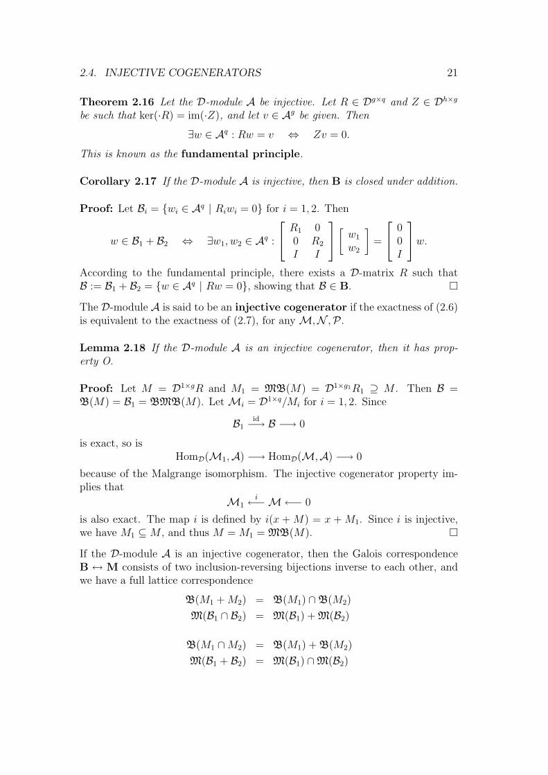
Corollary 2.17 If the D-module A is injective, then B is closed under addition.

Proof: Let Bi = wi ∈ Aq | Riwi = 0 for i = 1, 2. Then

w ∈ B1 + B2 ⇔ ∃w1, w2 ∈ Aq :

R1 00 R2

I I

[ w1

w2

]=

00I

w.According to the fundamental principle, there exists a D-matrix R such thatB := B1 + B2 = w ∈ Aq | Rw = 0, showing that B ∈ B.

The D-module A is said to be an injective cogenerator if the exactness of (2.6)is equivalent to the exactness of (2.7), for any M,N ,P .

Lemma 2.18 If the D-module A is an injective cogenerator, then it has prop-erty O.

Proof: Let M = D1×gR and M1 = MB(M) = D1×g1R1 ⊇ M . Then B =B(M) = B1 = BMB(M). Let Mi = D1×q/Mi for i = 1, 2. Since

B1id−→ B −→ 0

is exact, so isHomD(M1,A) −→ HomD(M,A) −→ 0

because of the Malgrange isomorphism. The injective cogenerator property im-plies that

M1i←−M←− 0

is also exact. The map i is defined by i(x + M) = x + M1. Since i is injective,we have M1 ⊆M , and thus M = M1 = MB(M).

If the D-module A is an injective cogenerator, then the Galois correspondenceB ↔ M consists of two inclusion-reversing bijections inverse to each other, andwe have a full lattice correspondence

B(M1 +M2) = B(M1) ∩B(M2)

M(B1 ∩ B2) = M(B1) + M(B2)

B(M1 ∩M2) = B(M1) + B(M2)

M(B1 + B2) = M(B1) ∩M(B2)


with B(0) = Aq, B(D1×q) = 0, M(0) = D1×q, M(Aq) = 0.

The following table lists some D-modules A that are relevant in systems theoryand that are injective cogenerators:

D AK[ d

dt] C∞(R,K),D′(R,K)

F[σ] FN

F[σ, σ−1] FZ

K[∂1, . . . , ∂n] C∞(Rn,K),D′(Rn,K)F[σ1, . . . , σn] F

Nn

F[σ1, . . . , σn, σ−11 , . . . , σ−1

n ] FZn

Example: Consider D = R[∂1, ∂2, ∂3] and A = C∞(R3,R). The statements

∃w ∈ A : grad(w) = v ⇔ curl(v) = 0

and∃w ∈ A3 : curl(w) = v ⇔ div(v) = 0

are two applications of the fundamental principle. Note that gradient, curl, anddivergence correspond to

Rgrad =

∂1

∂2

∂3

Rcurl =

0 −∂3 ∂2

∂3 0 −∂1

−∂2 ∂1 0

Rdiv =[∂1 ∂2 ∂3

].

♦

The following criteria make it easier to test whether a D-module A is an injectivecogenerator.

Theorem 2.19 The D-module A is injective if and only if for every sequence

0→ I → D,

where I ⊆ D is a left ideal, the sequence

0← HomD(I,A)← HomD(D,A)

is exact. This is known as Baer’s criterion [12, Ch. 1, §3].

Theorem 2.20 Let A be an injective D-module. Then A is a cogenerator if andonly if

HomD(M,A) = 0 ⇒ M = 0

for every finitely generated D-module M.

2.4. INJECTIVE COGENERATORS 23

Since D is left Noetherian, a finitely generated D-module M has the form M∼=D1×q/D1×gR for some suitable g, q and R ∈ Dg×q. To see this, suppose that Mhas q generators m1, . . . ,mq ∈ M. Then there exists a surjective D-linear mapπ from D1×q toM mapping each natural basis element ei to mi. The kernel of πis a left D-submodule of D1×q, and thus, it is also finitely generated, say it has ggenerators r1, . . . , rg ∈ D1×q. Let R be the matrix that contains these elements asrows. Then we have im(·R) = D1×gR = ker(π) and im(π) =M. The homomor-phism theorem implies that D1×q/ ker(π) ∼= im(π), that is, D1×q/D1×gR ∼= M.In other words, we have constructed an exact sequence

. . . −→ D1×g ·R−→ D1×q −→M −→ 0

and this procedure can be iterated, that is, the sequence can be extended to theleft. This is called a free resolution of M.

Therefore, if A is injective, the cogenerator property is equivalent to

B = w ∈ Aq | Rw = 0 = 0 ⇒ M = D1×q/D1×gR = 0

where we have used the Malgrange isomorphism. Note that M = 0 meansD1×gR = D1×q, i.e., there exists X ∈ Dq×g such that XR = I. However, wehave already seen in Corollary 2.13 that this implication is a consequence ofproperty O. Combining this with Lemma 2.18, we have the following result.

Theorem 2.21 Let A be an injective D-module. Then property O is equivalentto the cogenerator property.

Remark: Since D is left Noetherian, Baer’s criterion says in particular that itis sufficient to check injectivity for finitely generated modules in (2.6).

The proof of Baer’s criterion uses Zorn’s lemma which is equivalent to the axiomof choice. If this is to be avoided, an alternative formulation can be used. This isbased on the observation that for applications in systems theory, one deals onlywith sequences (2.6) of finitely generated modules. Thus, instead of requiring Ato be injective (which is equivalent to saying that HomD(·,A) is an exact functoron the category of left D-modules) it suffices, for systems theoretic purposes,to say that HomD(·,A) should be an exact functor on the category of finitelygenerated left D-modules.

The situation is simpler for the cogenerator property, because Theorem 2.20 doesnot rely on Zorn’s lemma. Its counterpart in the alternative formulation is: LetHomD(·,A) be an exact functor on the category of finitely generated left D-modules. Then HomD(·,A) is faithful (i.e., it reflects exactness) if and only ifHomD(M,A) = 0 implies M = 0 for all finitely generated left D-modules.


Chapter 3

Basic systems theoreticproperties

In this chapter, D is left Noetherian, and the D-module A is an injective cogen-erator. We consider an abstract linear system

B = w ∈ Aq | Rw = 0

and its system moduleM = D1×q/D1×gR,

where R ∈ Dg×q.

3.1 Autonomy

For 1 ≤ i ≤ q, consider the projection of B onto the i-th component

πi : B → A, w 7→ wi.

We say that wi is a free variable (or: an input) of B if πi is surjective. Thesystem B is called autonomous if it admits no free variables.

Interpretation: The surjectivity of πi means that for an arbitrary signal a ∈ A,we can always find q − 1 signals w1, . . . , wi−1, wi+1, . . . , wq ∈ A such that w :=(w1, . . . , wi−1, a, wi+1, . . . , wq)

T belongs to the system B. In this sense, the i-thcomponent of the signal vector w ∈ B is “free”, i.e., it can be chosen arbitrarily.

Compare this with the solvability condition for x = Ax + Bu discussed in theIntroduction: There, we required that for all u, there exists x such that x =Ax + Bu. Using the language from above, this says that u should be an input

25

26 CHAPTER 3. BASIC SYSTEMS THEORETIC PROPERTIES

in B = [xT , uT ]T | x = Ax + Bu. An autonomous system is a system withoutinputs, e.g., B = x | x = Ax.

Assumption: From now on, let D be a domain, that is, for all d1, d2 ∈ D, wehave

d1d2 = 0 ⇒ d1 = 0 or d2 = 0.

An element m ∈ M is called torsion (element) if there exists 0 6= d such thatdm = 0. The module M is called torsion (module) if all its elements aretorsion.

Lemma 3.1 If M is torsion, then B is autonomous.

Proof: If B is not autonomous, then there exists an exact sequence

B πi−→ A −→ 0.

Thus

M i←− D ←− 0

is also exact. This means that i is injective. Consider m := i(1) 6= 0. This is nota torsion element (if dm = 0 then di(1) = i(d) = 0 which implies d = 0 becausei is injective). Hence M is not torsion.

To obtain the converse direction of the implication of this lemma, we need thefollowing notion. One says that the domain D has the left Ore property if any0 6= d1, d2 ∈ D have a left common multiple, that is, there exist 0 6= c1, c2 ∈ Dsuch that c1d1 = c2d2. Inductively, it follows that every finite number of non-zeroelements of D has a left common multiple. The left Ore condition is equivalent tosaying that for all d1, d2 ∈ D, there exists (0, 0) 6= (c1, c2) ∈ D2 with c1d1 = c2d2.

Remark: If D is commutative, then it has the Ore property, because we maytake c1 = d2 and c2 = d1. However, the following theorem says that the assump-tions on D made so far (namely, D being a left Noetherian domain) are alreadysufficient to deduce the left Ore property [7, 12].

Theorem 3.2 If D is a left Noetherian domain, then it has the left Ore property.

Proof: Let 0 6= d1, d2 ∈ D. Consider the left ideals

In :=n∑i=0

Dd1di2.

3.1. AUTONOMY 27

Then we have an ascending chain I0 ⊆ I1 ⊆ I2 ⊆ . . ., which has to becomestationary according to the Noetherian property. Let n be the smallest integersuch that In+1 = In. Then

d1dn+12 =

n∑i=0

aid1di2

for some ai ∈ D. Re-arranging the summands, we obtain

a0d1 = (d1dn2 −

n∑i=1

aid1di−12 )d2

and hence we have constructed a left common multiple. If the coefficients werezero, we would have

d1dn2 =

n−1∑i=0

ai+1d1di2

and thus In = In−1, contradicting the minimality of n.

Lemma 3.3 The following are equivalent:

1. M is torsion.

2. B is autonomous.

Proof: Since “1⇒ 2” follows from the lemma above, it suffices to prove “2⇒ 1”:Assume thatM is not torsion. We first show that there exists an integer 1 ≤ i ≤ qsuch that [ei] is not torsion, where ei denotes the i-th natural basis vector of D1×q.

Suppose that all [ei] were torsion, say di[ei] = 0 for some di 6= 0. Now let m ∈Mbe given. Then m = [x] for some x ∈ D1×q, where [x] denotes the residue classof x modulo D1×gR. Then

m = [x] = [∑q

i=1 xiei] =∑q

i=1 xi[ei],

where xi ∈ D. Due to the left Ore property, there exist bi, 0 6= ci ∈ D withbidi = cixi. Similarly, let a := aici 6= 0 be a left common multiple of all ci. Then

am =∑axi[ei] =

∑aicixi[ei] =

∑aibidi[ei] = 0.

Thus M is torsion, contradicting the assumption.

Thus there is an exact sequence

0 −→ D i−→M


where i(1) = [ei]. Therefore,

0← HomD(D,A)← HomD(M,A)

is also exact, and thus, using the Malgrange isomorphism, so is

0←− A p←− B.

Thus p is surjective. However, p ≡ πi. This shows that B is not autonomous.


1. M is torsion.

2. There exists 0 6= d ∈ D and X ∈ Dq×g such that dI = XR.

3. B is autonomous.

Proof: It suffices to show “1⇒ 2⇒ 3”. IfM is torsion, then all [ei] are torsion,that is, there exists 0 6= di ∈ D such that di[ei] = 0. This means that diei = yiRfor some yi ∈ D1×g. Using the left Ore property, let d = cidi be a left commonmultiple of all di. Then dei = cidiei = ciyiR. Writing these equations in matrixform, we obtain dI = XR.

If dI = XR, then B ⊆ w | dw = 0, that is, every component wi of w ∈ Bsatisfies the scalar equation dwi = 0, where 0 6= d. However, it is a consequenceof property O (which holds since A is an injective cogenerator) that there is no0 6= d ∈ D with dA = 0, that is, no component of w is free. In other words, B isautonomous.

Corollary 3.5 Let D be commutative. Then B = w ∈ Aq | Rw = 0 is au-tonomous if and only if R has full column rank, i.e., rank(R) = q.

Remark: Over a commutative domain, the rank of a matrix can be defined asusual, that is, as the size of the largest non-singular submatrix. Note that anytwo representations of B have the same rank; this follows from Theorem 2.12.

Proof: Since adj(S)S = det(S)I holds for any square D-matrix S, and since afull column rank matrix contains a non-singular submatrix of full size, we have:R has full column rank if and only if there exists a D-matrix X and 0 6= d ∈ Dsuch that XR = dI. The rest follows from the theorem.

We would like to have a similar result for the non-commutative case as well.However, we cannot work with determinants and adjugate matrices any more.Some preparation is necessary.

3.1. AUTONOMY 29

Linear algebra over Ore domains

Let D be a domain. The left Ore property is necessary and sufficient for D toadmit a field of left fractions [3, p. 177]

K = d−1n | d, n ∈ D, d 6= 0.

In fact, the composition d−11 n1d

−12 n2 is explained by using the Ore property, which

yields an1 = bd2 for some a, b ∈ D, a 6= 0, and hence one puts

d−11 n1d

−12 n2 := (ad1)−1(bn2).

Of course, one has to show that this does not depend on the specific choice ofa, b.

Remark: This is the non-commutative generalization of the fact that everycommutative domain D can be embedded into its quotient field

K = nd| d, n ∈ D, d 6= 0,

for example, D = Z with K = Q, or D = K[t] with K = K(t).

For R ∈ Dg×q, consider V := RKq ⊆ Kg. This is a vector space over the skewfield K, and as such, it has a well-defined dimension

dim(V ) =: rank(R).

In fact, we should call this the column rank of R, but since it holds that

dim(RKq) = dim(K1×gR)

we have equality of row and column rank, just like in the classical case of linearalgebra over commutative fields, and therefore it is justified to simply speak ofthe rank of R. If D is a commutative domain, then this notion coincides withthe usual concept of the rank of a matrix.

Remark: The above statement should not be confused with rank(R) = rank(RT )which holds over commutative domains, but not in the non-commutative case, asillustrated by the following example.

Example: Let a, b ∈ D be such that ab 6= ba. Then the matrix

R =

[1 ba ab

]has rank 1 (as it would be in the commutative case), but its transpose

RT =

[1 ab ab

]has rank 2. ♦


Lemma 3.6 R has full column rank if and only if there exists a D-matrix X and0 6= d ∈ D such that XR = dI.

Proof: If XR = dI then

K1×qdI = K1×qXR ⊆ K1×gR ⊆ K1×q.

Since the leftmost and the rightmost vector space both have dimension q, we havedim(V ) = dim(K1×gR) = q, that is, R has rank q.

Conversely, assume that R has rank q. Let R1 be R after deletion of the firstcolumn. Since rank(R1) = q − 1 < g, there exists 0 6= x ∈ K1×g such thatxR1 = 0. Let x = [d−1

1 n1, . . . , d−1g ng]. Using the Ore property, we can write this

as x = d−1[n1, . . . , ng] =: d−1n for some n ∈ D1×g. Then nR1 = 0 and thusnR = [d, 0, . . . , 0]. There must be at least one choice of x that guarantees thatd 6= 0, otherwise this would be a contradiction to rank(R) = q. Let n be the firstrow of a matrix N . Proceeding like this with the remaining columns of R, weobtain NR = diag(d1, . . . , dq). Exploiting the Ore property once more, we canfind a diagonal matrix C such that CNR = dI, and we put X = CN .

This lemma is exactly what we need in order to generalize Corollary 3.5 to arbi-trary left Noetherian domains. Therefore we have proven the following result.

Theorem 3.7 B is autonomous if and only if R has full column rank.

3.2 Input-output structures

We still assume that D is a left Noetherian domain.

Let B = w ∈ Aq | Rw = 0 and p := rank(R). Since any two representationsof B possess the same rank, this number does not depend on the choice of therepresentation R of B, and therefore, it is a property of B, called the output-dimension of B.

Then there exist p columns of R that form a basis of V = RKq. Without lossof generality, we may re-arrange the columns of R such that the last p columnsare a basis of V . (This corresponds only to a permutation of the components ofw ∈ B.) Thus

R = [−Q,P ] with P ∈ Dg×p and rank(P ) = rank(R) = p.

This corresponds to a partition of w ∈ B according to

w =

[uy

].

3.3. CONTROLLABILITY 31

A partition constructed this way is called an input-output structure. Sincethe columns of Q belong to V , we get

Q = PH for some H ∈ Kp×m

where m := q − p, the input-dimension of B. This H is uniquely determined,and it called the transfer matrix of B with respect to the chosen input-outputstructure (note that in general, there are several input-output structures, corre-sponding to different choices of the basis of V ).

Theorem 3.8 Let B = w = [uT , yT ]T ∈ Am+p | Py = Qu be a system withinput-output structure. Then the transfer matrix H depends only on B and thechosen input-output structure (and not on the representation R). Moreover, wehave

∀u ∈ Am∃y ∈ Ap : Py = Qu

and this justifies the term “input-output structure”: The vector u consists of freevariables of B, and is therefore called an input. Moreover, the associated zero-input system Bu=0 = y ∈ Ap | Py = 0 is autonomous, and therefore, we call yan output.

Proof: Let R1 = [−Q1, P1] and R2 = [−Q2, P2] be two representations of B, andlet Q1 = P1H1 and Q2 = P2H2. Since R2 = XR1 and R1 = Y R2, this impliesP1(H1 −H2) = 0 and thus H1 = H2, because P1 has full column rank.

Let Z be such that ker(·P ) = im(·Z). According to the fundamental principle,

∃y ∈ Ap : Py = Qu ⇔ ZQu = 0.

However, since Q = PH, we have ZQ = ZPH = 0 and hence ZQu = 0 holds forany u ∈ Am.

Example: Let D = K[ ddt

] and A = C∞(R,K). Consider

B = [xT , uT ]T | x = Ax+Bu,

where A ∈ Kn×n and B ∈ Kn×m are given. Then R = [ ddtI − A,−B] has rank

p = n, and we may take P = ddtI−A, Q = B, and H = ( d

dtI−A)−1B ∈ K( d

dt)p×m.

♦

3.3 Controllability

We still assume that D is a left Noetherian domain.


An abstract linear system B = w ∈ Aq | Rw = 0 is called controllable if thereexists L ∈ Dq×l such that

B = w ∈ Aq | ∃` ∈ Al : w = L`.

This is called an image representation of B. We will see later on that forcertain choices of D and A, this definition coincides with the intuitive notion ofcontrollability as discussed in the Introduction.

Lemma 3.9 B is controllable if and only if R is a left syzygy matrix, that is,there exists a D-matrix L such that im(·R) = ker(·L).

Proof: B is controllable if and only if there exists L such that

Rw = 0 ⇔ ∃` ∈ Al : w = L`,

that is, kerA(R) = imA(L). Due to the injective cogenerator property, this isequivalent to im(·R) = ker(·L), that is, to R being a left syzygy matrix.

So far, we have only used the injective cogenerator property. Now we return toour assumption that D should be domain.

The module M is called torsion-free if it has no torsion elements except zero,that is, for all d ∈ D, m ∈M, we have

dm = 0 ⇒ d = 0 or m = 0.

For M = D1×q/M , this means that for all d ∈ D, x ∈ D1×q,

dx ∈M ⇒ d = 0 or x ∈M.

Lemma 3.10 If B is controllable, then M is torsion-free.

Proof: Let 0 6= d ∈ D and x ∈ D1×q be such that dx ∈ M = im(·R). SinceM = im(·R) = ker(·L) for some L, we have RL = 0 and hence dxL = 0. Since Dis a domain, this implies xL = 0, that is, x ∈ ker(·L) = M .

We need an additional assumption to obtain the converse direction of this impli-cation.

Assumption: From now on, let the domain D be Noetherian (i.e., both left andright Noetherian).


3.3. CONTROLLABILITY 33

1. B is controllable.

2. M is torsion-free.

3. R is a left syzygy matrix.

Proof: Since the equivalence of assertions 1 and 3 and the implication “1⇒ 2”follow from the above lemmas, it suffices to show “2⇒ 3”: LetM be torsion-free.Consider W = kerK(R) ⊆ Kq. This is an m-dimensional K-vector space, wherem = q − rank(R), which has a representation W = LKm for some L ∈ Kq×m.Using the right Ore property, we have L = Ld−1 for some L ∈ Dq×m. SinceRL = RLd−1 = 0, we may conclude that RL = 0. Consider ker(·L) ⊆ D1×q

and let Rc be such that im(·Rc) = ker(·L). We will show that im(·R) = im(·Rc),which yields the desired result. We have rank(R) = rank(Rc) and R = XRc forsome D-matrix X. Thus im(·R) ⊆ im(·Rc) and

K1×gR = K1×gXRc ⊆ K1×gcRc.

Since these vector spaces have the same dimension, they actually coincide, andthus we get Rc = GR for some K-matrix G. Using the left Ore property, we canwrite G = d−1N and thus dRc = NR. Let x be a row of Rc, then dx ∈ M , andthus, since M is torsion-free and d 6= 0, we must have x ∈ M . Thus Rc = Y Rfor some D-matrix Y .

Remark: The proof could be shortened considerably if we would use the factthat every finitely generated torsion-free module over a Noetherian domain can beembedded into a finitely generated free module, because then the exact sequence

D1×g ·R−→ D1×q π−→M = D1×q/im(·R)

and the embedding i :M→D1×l would yield an exact sequence

D1×g ·R−→ D1×q iπ−→ D1×l

and the map i π has to take the form ·L for some matrix L ∈ Dq×l.

However, the elementary proof from above gives a constructive method to find L.It also shows that without loss of generality, L has m columns, where m is theinput-dimension of the system. Note that alternatively, one could construct L asa matrix whose l columns generate the right D-module ker(R) ⊆ Dq, which isfinitely generated, because D is right Noetherian; but then we only have l ≥ m.Anyhow, the matrix Rc from the proof has interesting properties even when B isnot controllable. This is the topic of the next section.



B = [xT , uT ]T | x = Ax+Bu,


where A ∈ Kn×n and B ∈ Kn×m are given. Then R = [ ddtI − A,−B] and

M = D1×(n+m)/D1×nR.

One can show that M is torsion-free if and only if rank[B,AB, . . . , An−1B] = n,thus recovering the controllability condition from the Introduction. ♦

3.4 The controllable part of a system

We still assume that D is a Noetherian domain.

Theorem 3.12 There exists a uniquely determined largest controllable subsystemBc of B, that is, Bc ⊆ B, Bc is controllable, and if B1 is another controllablesubsystem of B, then B1 ⊆ Bc. The system Bc is called the controllable partof B. We have B = Bc if and only if B is controllable.

Proof: Consider the matrix Rc constructed above and set

Bc = w ∈ Aq | Rcw = 0.

By construction, R = XRc, that is, Bc ⊆ B, and Rc is a left syzygy matrix, thatis, Bc is controllable.

Let B1 = w ∈ Aq | R1w = 0 be another controllable subsystem of B, thenR = Z1R1 and im(·R1) = ker(·L1) for some D-matrices Z1, L1. Recall thatby construction, dRc = NR for some 0 6= d ∈ D and a D-matrix N . ThusdRcL1 = NRL1 = NZ1R1L1 = 0, and since D is a domain, we may concludethat RcL1 = 0. Therefore we must have Rc = Z2R1, that is, B1 ⊆ Bc.

The torsion part tM of M is the set of all torsion elements of M, that is,

tM = m ∈M | ∃0 6= d ∈ D : dm = 0.

Theorem 3.13 tM is a left submodule ofM, the moduleM/tM is torsion-free,and we have the Malgrange isomorphism

Bc ∼= HomD(M/tM,A).

In particular, B is autonomous if and only if Bc = 0.

Proof: Let m1,m2 ∈ tM, that is, d1m1 = d2m2 = 0 for some 0 6= d1, d2 ∈ D.Since d1 and d2 have a left common multiple 0 6= d = c1d1 = c2d2, we obtaind(m1 +m2) = c1d1m2 + c2d2m2 = 0, showing that m1 +m2 ∈ tM.

3.4. THE CONTROLLABLE PART OF A SYSTEM 35

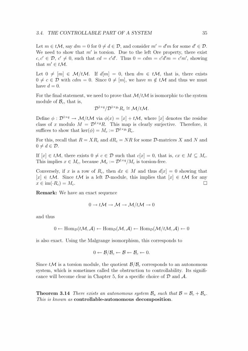
Let m ∈ tM, say dm = 0 for 0 6= d ∈ D, and consider m′ = d′m for some d′ ∈ D.We need to show that m′ is torsion. Due to the left Ore property, there existc, c′ ∈ D, c′ 6= 0, such that cd = c′d′. Thus 0 = cdm = c′d′m = c′m′, showingthat m′ ∈ tM.

Let 0 6= [m] ∈ M/tM. If d[m] = 0, then dm ∈ tM, that is, there exists0 6= c ∈ D with cdm = 0. Since 0 6= [m], we have m /∈ tM and thus we musthave d = 0.

For the final statement, we need to prove thatM/tM is isomorphic to the systemmodule of Bc, that is,

D1×q/D1×gcRc∼=M/tM.

Define φ : D1×q → M/tM via φ(x) = [x] + tM, where [x] denotes the residueclass of x modulo M = D1×gR. This map is clearly surjective. Therefore, itsuffices to show that ker(φ) = Mc := D1×gcRc.

For this, recall that R = XRc and dRc = NR for some D-matrices X and N and0 6= d ∈ D.

If [x] ∈ tM, there exists 0 6= c ∈ D such that c[x] = 0, that is, cx ∈ M ⊆ Mc.This implies x ∈Mc, because Mc := D1×q/Mc is torsion-free.

Conversely, if x is a row of Rc, then dx ∈ M and thus d[x] = 0 showing that[x] ∈ tM. Since tM is a left D-module, this implies that [x] ∈ tM for anyx ∈ im(·Rc) = Mc.

Remark: We have an exact sequence

0→ tM→M→M/tM→ 0

and thus

0← HomD(tM,A)← HomD(M,A)← HomD(M/tM,A)← 0

is also exact. Using the Malgrange isomorphism, this corresponds to

0← B/Bc ← B ← Bc ← 0.

Since tM is a torsion module, the quotient B/Bc corresponds to an autonomoussystem, which is sometimes called the obstruction to controllability. Its signifi-cance will become clear in Chapter 5, for a specific choice of D and A.

Theorem 3.14 There exists an autonomous system Ba such that B = Bc + Ba.This is known as controllable-autonomous decomposition.


Remark: Note that Ba is not uniquely determined, and that it is not possible,in general, to choose Ba such that the sum Ba + Bc is direct.

Proof: Choose an input-output structure and set B = [uT , yT ]T | Py = Qu,that is R = [−Q,P ] = XRc. Partition Rc = [−Qc, Pc] correspondingly, then thisis an input-output structure of Bc = [uT , yT ]T | Pcy = Qcu.

Let Ba := [uT , yT ]T | Py = 0, u = 0. This is autonomous and contained in B.Thus Bc + Ba ⊆ B.

For the converse, let [uT , yT ]T ∈ B. There exists a solution y1 to Pcy1 = Qcu.Write [

uy

]=

[uy1

]+

[0

y − y1

].

The first summand is in Bc, and the second is in Ba, because

P (y − y1) = Py −XPcy1 = Qu−XQcu = Qu−Qu = 0

for all u.

Example: Let A ∈ Kn×n and B ∈ Kn×m. Then there exists a non-singularT ∈ Kn×n such that

T−1AT =

[A1 A2

0 A3

]and T−1B =

[B1

0

]where A1 ∈ Kn1×n1 , B1 ∈ Kn1×m, and (A1, B1) is controllable, that is,

rank[B1, A1B1, . . . , An1−11 B1] = n1.

This is the so-called Kalman controllability decomposition. Therefore wemay assume without loss of generality that

B = [xT1 , xT2 , uT ]T | x1 = A1x1 + A2x2 +B1u, x2 = A3x2.

Then

Bc = [xT1 , xT2 , uT ]T | x2 = 0, x1 = A1x1 +B1u

and

Ba = [xT1 , xT2 , uT ]T | u = 0, x1 = A1x1 + A2x2, x2 = A3x2.

Note that Bc ∩ Ba 6= 0, but in this example, it is possible to find another au-tonomous system B′a such that B = Bc ⊕ B′a. ♦

3.5. OBSERVABILITY 37

3.5 Observability

Let B be an abstract linear system in which the representation matrix is par-titioned as R = [R1, R2]. Let the signal vector w be partitioned accordingly.Then

B = [wT1 , wT2 ]T ∈ Aq1+q2 | R1w1 +R2w2 = 0.One says that w1 is observable from w2 in B if w1 is uniquely determined by w2

and the fact that R1w1 + R2w2 = 0. This means that R1w′1 + R2w2 = 0 and

R1w1 +R2w2 = 0 should imply that w1 = w′1. Equivalently,

B1 := w1 ∈ Aq1 | R1w1 = 0 = 0.

The following theorem is a direct consequence of Corollary 2.13.

Theorem 3.15 The subsignal w1 is observable from w2 if and only if R1 is leftinvertible, that is, there exists a D-matrix X such that I = XR1.

A latent variable description of B takes the form

B = w ∈ Aq | ∃` ∈ Al : Rw = M`

where R ∈ Dg×q and M ∈ Dg×l. According to the fundamental principle, this isindeed an abstract linear system, i.e., we can construct a kernel representation.One is particularly interested in the question whether the latent variables ` areobservable from the manifest variables w in the associated “full” system

Bf = [`T , wT ]T ∈ Al+q | M` = Rw.

The theorem above tells us that this is the case if and only if M is left invertible.Then we have

B = w ∈ Aq | ∃!` ∈ Al : Rw = M`,which called an observable latent variable description.



B = [uT , yT ]T ∈ Am+p | ∃x ∈ An : x = Ax+Bu, y = Cx+Du.

This is the input-output system associated to the state space system

x = Ax+Bu

y = Cx+Du,

and the full system consists of all [xT , uT , yT ]T that satisfy these equations. Here,the latent variables correspond to the state x, and the input u and the output y


are considered as manifest variables. Since the state space equations can berewritten as [

B 0−D I

] [uy

]=

[ddtI − AC

]x,

we see that observability amounts to the left invertibility of

M =

[ddtI − AC

]which is equivalent to the classical observability criterion, which says that

K =

CCA

...CAn−1

should have rank n. ♦

Chapter 4

One-dimensional systems

4.1 Ordinary differential equations with ratio-

nal coefficients

Let D = K[ ddt

], where K = K(t) is the field of rational functions. Then D is thering of linear ordinary differential operators with rational coefficients.

Let A denote the set of all functions that are smooth except for a finite numberof points, that is, for each a ∈ A there exists a finite set E(a) ⊂ R such thata ∈ C∞(R \ E(a),K). Then A is a K-vector space and a left D-module. We willidentify functions whose values coincide almost everywhere.

Recall that D is not commutative, because

d

dtta = a+ t

d

dta for all a ∈ A

and thus ddtt = 1 + t d

dt. More generally, for k ∈ K, we have

d

dtk = k′ + k

d

dt

and, proceeding inductively,

di

dtik =

i∑j=0

(ij

)k(i−j) d

j

dtj.

The ring D is a domain, and any element 0 6= d ∈ D can be uniquely written inthe form

d = an(t)dn

dtn+ . . .+ a1(t)

d

dt+ a0(t)

39

40 CHAPTER 4. ONE-DIMENSIONAL SYSTEMS

where n ∈ N, ai ∈ K, and an 6= 0. The number n is called the degree of d, andan is called the leading coefficient of d. If the leading coefficient equals one, wesay that d is monic.

Theorem 4.1 [7, Ch. 1] The ring D is simple (that is, the only ideals that areboth right and left ideals are the trivial ones, i.e., 0 and D itself) and it is a leftand right principal ideal domain (that is, every left ideal and every right ideal canbe generated by one single element).

Proof: Let I be a non-zero right and left ideal in D. Let

n := mindeg(f) | 0 6= f ∈ I.

Then I contains an element d of degree n. If n = 0, we have I = D, and we’refinished. If n ≥ 1, consider the element kd − dk ∈ I, where k ∈ K. We have(writing D := d

dtto simplify the notation)

kd− dk = kn∑i=0

aiDi −

n∑i=0

aiDik

= k

n∑i=0

aiDi −

n∑i=0

ai

i∑j=0

(ij

)k(i−j)Dj

= k

n∑i=0

aiDi −

n∑i=0

n∑j=i

aj

(ji

)k(j−i)Di.

The coefficient at Dn equals kan − ank, which is zero (since K is commutative).Hence the degree of kd − dk is at most n − 1. However, since n was chosen tobe minimal, we must have kd − dk = 0. Then the coefficient at Dn−1 has tovanish. This coefficient is given by kan−1 − an−1k − annk′ = −annk′. Thus wehave shown that for all k ∈ K, we have k′ = 0. This is clearly absurd, and thuswe have shown that the assumption n ≥ 1 must be false.

Now let I be a non-zero left ideal of D. Define n as above, and let d ∈ I havedegree n. Without loss of generality, let d be monic. We show that I = Dd. SinceDd ⊆ I is obvious, it suffices to show that I ⊆ Dd. We do this by inductionon the degree of f ∈ I. If deg(f) = n, we consider f − fnd whose degree is lessthan n. Thus it must be zero, showing that f = fnd ∈ Dd. Suppose that we haveshown the statement for all f ∈ I of degree n, n+ 1, . . . ,m− 1. Consider f ∈ Iwith deg(f) = m. Then f − fmDm−nd has degree less than m. By the inductivehypothesis, it has to be in Dd, which implies f ∈ Dd.

The statement for right ideals is proven similarly.

4.1. ORDINARY DIFFERENTIAL EQUATIONS 41

Remark: In fact, D is even a left and right Euclidean domain, with means thatwe have a left and right “division with remainder”: For all 0 6= d ∈ D andn ∈ D there exist q, r ∈ D such that n = qd + r, where we have either r = 0 ordeg(r) < deg(d). Similarly, we have n = dq1 + r1.

Anyhow, D is left and right Noetherian and thus it has the left and right Oreproperty. Thus it admits a skew field of fractions K, and the rank of a D-matrixis well-defined. A matrix U ∈ Dg×g is called unimodular if there exists a matrixU−1 ∈ Dg×g with UU−1 = U−1U = I.

Theorem 4.2 (Jacobson form) [8, Ch. 3], [5, Ch. 8.1] Let R ∈ Dg×q. Thenthere exist unimodular matrices U and V such that

URV =

[D 00 0

]where D = diag(1, . . . , 1, d) ∈ Dp×p for some 0 6= d ∈ D, and p := rank(R).

Since D is even a Euclidean domain, the transformation matrices U and V canbe obtained by performing elementary row and column operations.

In the following proof, we use the following standard facts from ODE theory: Theinitial value problem x(t) = A(t)x(t) + b(t), x(t0) = x0, where A ∈ C∞(I,Kn×n)and b ∈ C∞(I,Kn) for some open interval I ⊆ R, has a unique solution for anychoice of t0 ∈ I and x0 ∈ Kn. This solution is defined on all of I and it is smooth,that is, x ∈ C∞(I,Kn). The solution set of the associated homogeneous equationx(t) = A(t)x(t) is a K-vector space of dimension n.

Moreover, the tests for the injective cogenerator property given in Chapter 2can be simplified in the case where D is a left principal ideal domain. A leftD-module A is injective if and only if for all 0 6= d ∈ D and all u ∈ A, thereexists y ∈ A such that dy = u. An injective module is a cogenerator if and only ifHomD(D/Dd,A) = 0 implies D/Dd = 0 for any d ∈ D. In view of the Malgrangeisomorphism, this is equivalent to saying that w ∈ A | dw = 0 = 0 implies thatd is left invertible. However, since D is a domain, left and right invertibility ofd ∈ D are equivalent. Moreover, in D = K(t)[ d

dt], an element d ∈ D is a unit if

and only if d ∈ K(t) \ 0, that is, deg(d) = 0.

Theorem 4.3 The left D-module A is an injective cogenerator.

Proof: For injectivity, we need to prove: For every 0 6= d ∈ D and every u ∈ A,there exists y ∈ A such that dy = u. Let d = an(t) d

n

dtn+ . . .+ a0(t) be given, with

an 6= 0. If n = 0, there is nothing to prove, so let us assume that n ≥ 1. Since K


is a field, one may assume that an = 1. Then dy = u can be rewritten as a firstorder system

x(t) = A(t)x(t) +Bu(t),

where x = [y, y, . . . , y(n−1)]T and

A =

0 1...

. . .

0 1−a0 · · · · · · −an−1

∈ Kn×n and B =

0...01

∈ Kn.

Let E(d) be the finite set of all poles of the rational coefficients ai of d. LetE(y) := E(u) ∪ E(d) = t1, . . . , tk with t1 < . . . < tk. On every interval I ⊆ Rof the form (ti, ti+1) or (−∞, t1) or (tk,∞), it holds that A|I and u|I are smooth.Therefore, there exists a smooth solution xI : I → K

n to x = Ax + Bu on eachof these intervals. By concatenating them (i.e., by setting x|I := xI), one gets asolution x ∈ An and thus y = x1 ∈ A.

For the cogenerator property, it has to be shown that if for some d ∈ D, theequation dy = 0 possesses only the zero solution, then d ∈ K \ 0. Assumeconversely that deg(d) = n ≥ 1. The one can rewrite dy = 0 as x(t) = A(t)x(t).On each of the intervals I from above, the solution set of this is an n-dimensionalsubspace of C∞(I,Kn), in particular, there exist non-zero solutions. Concatenat-ing them, we obtain a non-zero solution x ∈ An. If y = x1 were identically zero,then x = [y, y, . . . , y(n−1)]T would also be identically zero, a contradiction.

4.2 Rationally time-varying systems

Let R ∈ Dg×q be given. The abstract linear system

B = w ∈ Aq | Rw = 0

is the solution space of the linear system of rational-coefficient ordinary differen-tial equations Rw = 0.

Let

URV =

[D 00 0

]be the Jacobson form of R, and let W := V −1 ∈ Dq×q. Since Rw = 0 is equivalentto URw = URVWw = 0, there is an isomorphism of Abelian groups

B ∼= B := w ∈ Aq | [D, 0]w = 0 (4.1)

w 7→ w := Ww

4.2. RATIONALLY TIME-VARYING SYSTEMS 43

where

B = w ∈ Aq | w1 = . . . = wp−1 = 0, dwp = 0 (4.2)

is fully decoupled, since D = diag(1, . . . , 1, d).

Consider the system module M = D1×q/D1×gR. According to the Jacobsonform, there is an isomorphism of left D-modules

M ∼= M = D1×q/D1×p[D, 0]

[x] 7→ [xV ]

where [·] denotes the residue class of an element of D1×q inM or M, respectively.Thus we have

M∼= D/Dd×D1×m = D/Dd⊕D1×m (4.3)

wherem := q−p and p = rank(R). The moduleD/Dd is isomorphic to the torsionsubmodule tM of M. The module M/tM∼= D1×m is not only torsion-free, buteven free.

The decomposition (4.3) induces an isomorphism of Abelian groups

B ∼= y ∈ A | dy = 0 ⊕ Am, (4.4)

because

HomD(D/Dd,A) ∼= y ∈ A | dy = 0

according to the Malgrange isomorphism, and

HomD(D1×m,A) ∼= Am.

Of course, the existence of the isomorphism (4.4) can also be seen directly from(4.1) and (4.2). The details of this decomposition will be investigated in Theo-rem 4.11 below.

Existence of full row rank representations

Corollary 4.4 Let B = w ∈ Aq | Rw = 0 for some R ∈ Dg×q. Then B can berepresented by a matrix with full row rank.

Proof: Without loss of generality, let R 6= 0 (the system B = Aq can be repre-sented by the empty matrix, which has full row rank by convention). Let

URV =

[D 00 0

]


be the Jacobson form of R. Partition

W = V −1 =

[W1

W2

](4.5)

according to the partition of the Jacobson form. Since U is unimodular, Rw = 0is equivalent to URw = 0. Thus R := DW1 also represents B, and it has full rowrank.

Equivalence of representations

Corollary 4.5 Let R1, R2 be two D-matrices with the same number of columns,and let B1,B2 be the associated systems. We have B1 ⊆ B2 if and only if R2 =XR1 for some D-matrix X. If B1 = B2, then R1 and R2 have the same rank. IfR1 and R2 have full row rank, then B1 = B2 if and only if R2 = UR1 for someunimodular matrix U .

Proof: It suffices to show the final statement. If B1 = B2, then R2 = XR1 andR1 = Y R2, which shows that R1 and R2 have the same rank. If additionally, R1

and R2 both have full row rank, then they have the same number of rows, whichimplies that X and Y are square, and in fact, we must have X = Y −1 showingthat the matrices are unimodular.

Elimination of latent variables

Corollary 4.6 Consider

B = w ∈ Aq | ∃` ∈ Al : Rw = M`

where R ∈ Dg×q and M ∈ Dg×l. Then there exists a kernel representation of B.

Proof: This follows from the fundamental principle.

Input-output structures and autonomy

Let R ∈ Dp×q be a full row rank representation of B. Then there exists a p × psubmatrix P of R of full rank. Without loss of generality, arrange the columnsof R such that R = [−Q,P ]. Let w = [uT , yT ]T be partitioned accordingly. This


is called an input-output structure of B, and H = P−1Q ∈ Kp×m is called itstransfer matrix. The term input-output structure is justified by the fact that

∀u ∈ Am∃y ∈ Ap : Py = Qu.

Note that the exactness of

0 −→ D1×p ·P−→ D1×p

implies the exactness of

0←− Ap P←− Ap

which says that P : Ap → Ap is even surjective, i.e., for all v ∈ Ap there existsy ∈ Ap such that Py = v. In particular, this is true for v = Qu. Then onesays that u is a vector of free variables of B. Recall that a system without freevariables is called autonomous.

Corollary 4.7 The following are equivalent:

1. B is autonomous.

2. B can be represented by a square matrix of full rank.

3. M is torsion.

Proof: The equivalence of assertions 1 and 3 is known from the previous chap-ter. We also know that these two assertions are equivalent to the fact that anyrepresentation matrix has full column rank. Therefore it suffices to show that“1 ⇒ 2”: However, since representations with full row rank do always exist, arepresentation of an autonomous system can be assumed to have both full rowand full column rank. Then it must be square of full rank.

Now we can give an analytic interpretation of autonomy.


1. B is autonomous.

2. There exists a finite set E ⊂ R such that for all open intervals I ⊆ R \ E,and all w ∈ B that are smooth on I, we have

w|J = 0 ⇒ w|I = 0

for all open intervals J ⊆ I.


Proof: If B is autonomous, then B ∼= y ∈ A | dy = 0 for some 0 6= d ∈ D.If d ∈ K, then B = 0 and the result follows. Otherwise, set E := E(d) andlet I ⊆ R \ E. Similarly as above, the equation dy = 0 can be rewritten asx(t) = A(t)x(t), where x = [y, . . . , y(n−1)]T , and A is smooth on I. If y is smoothon I, then so is x. If y|J = 0 for some open interval J ⊆ I, then x|J = 0, and thusthe solution x of the homogeneous equation x = Ax must be identically zero onall of I (due to the uniqueness of the solution of the initial value problem x = Ax,x(t0) = 0, where t0 ∈ J), and hence this holds also for y = x1.

If B is not autonomous, then it contains free variables. Therefore w|J = 0 doesnot imply the vanishing of w on a larger set I, because the free variables can bechosen arbitrarily, in particular, they can take non-zero values arbitrarily closeto J .

Examples:

• Consider R = t ddt

+ 1, which corresponds to the differential equation

w(t) + 1tw(t) = 0.

On every open interval I ⊂ R \ 0 on which w is smooth, it holds thatw(t) = c

tfor some c ∈ K. Thus every solution has a singularity at zero,

that is, 0 ∈ E(w) for all w ∈ B.

In spite of its singularity at zero, the function w(t) = 1t, defined on R \ 0,

can be interpreted as a distribution on R, that is, there exists W ∈ D′(R,K)such that W and the regular distribution generated by w on R \ 0 assignthe same value to each test function whose support is in R \ 0.

• Consider R = t3 ddt

+ 1, which corresponds to

w(t) + 1t3w(t) = 0.

On every open interval I ⊂ R \ 0 on which w is smooth, we have w(t) =

ce1

2t2 for some c ∈ K. Again, we have 0 ∈ E(w) for all solutions w.

In contrast to the previous example, it is known that there exists no distri-bution W ∈ D′(R,K) that coincides with the regular distribution generated

by w(t) = e1

2t2 on R \ 0. This shows that the set of distributions is notan injective cogenerator as a K[ d

dt]-module (however, it is if K is replaced

by the field of constants K).

• Consider R = t ddt− 1. Any w of the form w(t) = ct, c ∈ K, solves the

resulting equation Rw = 0. Therefore, there exist solutions that are smoothon all of R (that is, E(w) = ∅), but also any function of the form

w(t) =

c1t for t < 0c2t for t > 0


where c1, c2 ∈ K is a solution to Rw = 0 in A (and if c1 6= c2, then0 ∈ E(w)).

• Consider R = t3 ddt−1. Here we have solutions of the form w(t) = ce−

12t2 for

c ∈ K. These solutions are smooth on all of R, even if we select differentvalues of the constant c for t > 0 and t < 0.

• Consider R = (1− t2)2 ddt

+ 2t. A solution is given by

w(t) =

e− 1

1−t2 for − 1 < t < 10 otherwise

which happens to be smooth on all of R. This example shows that the au-tonomous equation Rw = 0 possesses non-zero solutions of compact support(which is impossible in the constant coefficient case). ♦

Image representations and controllability


1. B admits an image representation.

2. B admits a right invertible kernel representation matrix.

3. M is torsion-free, or equivalently, free.

Proof: The system B = Aq with its module M = D1×q satisfies all three condi-tions, if we use that it can be represented by the empty matrix, which we declareright invertible, as a convention. Therefore, assume that B 6= Aq, that is, R 6= 0.

It follows from the decomposition (4.3) that M is torsion-free if and only if itis free. Thus the equivalence of the first and third condition is known from theprevious chapter.

Therefore it suffices to prove: Provided that R has full row rank,M is torsion-freeif and only if R is right invertible. For a full row rank matrix R, the Jacobsonform is URV = [D, 0], where D = diag(1, . . . , 1, d), with d 6= 0. It is easy tosee that R is right invertible if and only if its Jacobson form is right invertible,and for the Jacobson form, right invertibility is equivalent to d ∈ K. On theother hand, this is precisely the criterion for the vanishing of the torsion parttM∼= D/Dd of M.


Remark: The assertions of the theorem are equivalent to the statement that theelement 0 6= d that appears in the Jacobson form of a kernel representation Rof B has degree zero, that is, d ∈ K. Note that since tM∼= D/Dd, the degree of dcorresponds to the K-dimension of tM, and therefore, it is uniquely determinedby M, or B, equivalently. If 0 6= d ∈ K, we may put d = 1, without loss ofgenerality, and then the Jacobson form of a full row rank representation R ∈ Dp×qof B takes the form URV = [I, 0].

Now we can give an interpretation of the controllability notion from the pre-vious chapter (namely, the existence of an image representation) in terms of aconcatenation property of the system trajectories.

The system B is called concatenable if for all w1, w2 ∈ B and all but finitelymany t0 ∈ R, there exists w ∈ B, an open interval t0 ∈ I ⊆ R such that w1, w2, ware smooth on I, and τ > 0 with t0 + τ ∈ I such that

w(t) =

w1(t) if t < t0w2(t) if t > t0 + τ

for all t ∈ I.

Theorem 4.10 B is concatenable if and only if it is controllable.

Proof: Let B = w ∈ Aq | ∃` ∈ Al : w = L` and let w1 = L`1, w2 = L`2 ∈ B begiven. Let t0 be in R \ (E(`1)∪E(`2)∪E(L)). Then there exists an open intervalt0 ∈ I ⊆ R such that `1, `2 and w1, w2 are smooth on I. Choose τ > 0 and let `be a smooth function on I with

`(t) =

`1(t) if t < t0`2(t) if t > t0 + τ.

Then w := L` has the desired property. This direction of the proof can also beseen directly from the fact that if B has an image representation, then B ∼= Am,and Am has the required concatenability property.

For the converse, it suffices to show that Ba = w ∈ A | dw = 0, whered ∈ D \ K, is not concatenable. Let w1 be the zero solution, and let w2 be anon-zero solution. Then there exists an open interval J ⊆ R \ E(d) on which w2

is smooth and does not vanish. Let t0 ∈ J . Suppose that w were a connectingtrajectory. Then w is smooth on some open neighborhood I ⊆ J of t0. On theother hand, since Ba is autonomous, w(t) = w1(t) = 0 for all t ∈ I with t < t0implies that w(t) = 0 for all t ∈ I. This contradicts w(t) = w2(t) 6= 0 for all t ∈ Iwith t > t0 + τ .


Theorem 4.11 There exists a largest controllable subsystem Bc of B, and B canbe decomposed into a direct sum

B = Ba ⊕ Bc

where Ba is autonomous.

This decomposition corresponds to (4.3). Note that

Ba ∼= HomD(tM,A) ∼= HomD(D/Dd,A) ∼= y ∈ A | dy = 0

andBc ∼= HomD(M/tM,A) ∼= HomD(D1×m,A) ∼= Am.

Proof: Let R be a full row rank representation of B, and let URV =[D 0

]be the Jacobson form of R. Let W = V −1 be partitioned as in (4.5). Then

w ∈ B ⇔[D 0

]Ww = DW1w = 0.

Let V = [V1, V2] be partitioned accordingly and set

Bc = w ∈ Aq | W1w = 0= w ∈ Aq | ∃` ∈ Am : w = V2`.

The second equality follows from W = V −1, which implies W1V2 = 0 and V1W1 +V2W2 = I, from which one can conclude that im(·W1) = ker(·V2). Then Bc ⊆ B iscontrollable. If B1 is another controllable subsystem of B, then B1 ⊆ Bc. Define

Ba = w ∈ Aq | DW1w = 0 and W2w = 0.

Then Ba ⊆ B is autonomous, and B = Ba⊕Bc, where the decomposition is givenby w = V1W1w + V2W2w.

Observability

Let R = [R1, R2] and let w = [wT1 , wT2 ]T be partitioned accordingly. One says

that w1 is observable from w2 in R1w1 + R2w2 = 0 if w1 is uniquely determinedby w2. Due to linearity, this is equivalent to

B1 := w1 ∈ Aq1 | R1w1 = 0 = 0.

Theorem 4.12 Let B be given by Rw = R1w1+R2w2 = 0. Then w1 is observablefrom w2 if and only if R1 is left invertible.


4.3 Time-invariant case

All the results of Section 4.2 hold also for the constant coefficient case, thatis, D = K[ d

dt] and A = C∞(R,K), with some slight modifications of the proofs

where necessary. The main difference is that the matrix D from the Jacobsonform (which is then the Smith form) has the form D = diag(d1, . . . , dp). Thusthe torsion submodule tM of M is isomorphic to D/Dd1 ⊕ · · · ⊕ D/Ddp. Still,the characterizations of Theorem 4.9 are equivalent to D = I. Similarly, Ba isisomorphic to y ∈ Ap | diyi = 0 for 1 ≤ i ≤ p. The quotient field of D is thefield of rational functions K = K( d

dt), and thus transfer matrices are rational.

The concepts of autonomy and controllability, formulated in terms of the trajec-tories, become simpler:

• B is autonomous if for all w ∈ B and all open intervals J ⊆ R, we have

w|J = 0 ⇒ w = 0.

• B is controllable if for all w1, w2 ∈ B, and all t0 ∈ R, there exists w ∈ Band τ > 0 such that

w(t) =

w1(t) if t < t0w2(t) if t > t0 + τ

for all t ∈ R. Here, we can put t0 = 0 without loss of generality.

Chapter 5

Multi-dimensional systems

In this chapter,

D = K[∂1, . . . , ∂n] and A = C∞(Rn,K),

that is, we deal with systems of linear partial differential equations with con-stant coefficients (note that linear ordinary differential equations with constantcoefficients are included as the special case n = 1) and their smooth solutions.

The ring D is a commutative Noetherian domain, and the D-module A is aninjective cogenerator. Therefore the theory of Chapter 3 is directly applicable.However, D is not a principal ideal domain (unless n = 1), and therefore, thereexists no analogue of the Smith form for n ≥ 2. Thus the results of the previouschapter do not translate to this setting, for example, not every system has a fullrow rank representation.

5.1 Interpretation of autonomy and controlla-

bility

Let B = w ∈ Aq | Rw = 0, where R ∈ Dg×q.

Lemma 5.1 Let B be autonomous. If w ∈ B has compact support, then w = 0.

Proof: Let B = w ∈ Aq | Rw = 0 be autonomous. This means that R hasfull column rank. Let w ∈ B have compact support. Then w has a well-definedFourier transform w := Fw, defined by

w(ξ) =

∫Rn

w(x)e−i〈x,ξ〉dx,

51

52 CHAPTER 5. MULTI-DIMENSIONAL SYSTEMS

where 〈x, ξ〉 =∑n

i=1 xiξi, and w is an analytic function of ξ ∈ Rn. The Fouriertransform of Rw = 0 yields R(iξ)w(ξ) = 0. This can be interpreted as a linearequation over the field of meromorphic functions. Since R(iξ) has full columnrank, we obtain w = 0, and hence, using the inverse Fourier transform, w = 0.

Theorem 5.2 The following are equivalent [19]:

1. B is controllable, i.e., it possesses an image representation.

2. For all open sets U1, U2 ⊂ Rn, with U1 ∩ U2 = ∅, and for all w1, w2 ∈ B,there exists w ∈ B such that

w(x) =

w1(x) if x ∈ U1

w2(x) if x ∈ U2.

3. For all 0 < r1 < r2 and for all w1, w2 ∈ B, there exists w ∈ B such that

w(x) =

w1(x) if x ∈ U1

w2(x) if x ∈ U2,

where

U1 = x ∈ Rn | ‖x‖ < r1 and U2 = x ∈ Rn | ‖x‖ > r2,

and ‖ · ‖ denotes the Euclidean norm.

Proof: “1 ⇒ 2”: Suppose that B possesses an image representation

B = w ∈ Aq | ∃` ∈ Al : w = L`.

Let Ui and wi = L`i for i = 1, 2 be given. It is a fundamental property ofA = C∞(R,K) that for any open sets U1, U2 whose closures are disjoint, thereexists a smooth function χ with [23, §1, VIII]

χ(x) =

1 if x ∈ U1

0 if x ∈ U2.

Set ` := χ`1 + (1− χ)`2 ∈ Al. Then

`(x) =

`1(x) if x ∈ U1

`2(x) if x ∈ U2.

Set w := L`, then w ∈ B has the desired properties.

Since assertion 3 is obviously a special case of assertion 2, it suffices to show that“3 ⇒ 1”: If B is not controllable, then Bc ( B, that is, there exists w0 ∈ B with

5.1. INTERPRETATION OF AUTONOMY AND CONTROLLABILITY 53

v0 := Rcw0 6= 0, but dv0 = 0 (recall that dRc = NR for some 0 6= d ∈ D andsome D-matrix N). Let x0 be such that v0(x0) 6= 0. Choose r2 > r1 > ‖x0‖ andlet U1, U2 be the corresponding sets from assertion 3. We show that there existsno w ∈ B such that

w(x) =

w0(x) if x ∈ U1

0 if x ∈ U2.

Indeed, if this were the case, then v := Rcw would be a non-zero compact sup-port element of the autonomous system v ∈ A | dv = 0, which is impossibleaccording to the lemma above.

Lemma 5.3 If B 6= 0 is controllable, then it contains a non-zero trajectory withcompact support.

Proof: Let 0 6= w0 ∈ B. Let x0 be such that w0(x0) 6= 0. Let r2 > r1 > ‖x0‖ andlet U1, U2 be as defined above. By controllability, there exists w ∈ B such that

w(x) =

w0(x) if x ∈ U1

0 if x ∈ U2.

Then w is non-zero and it has compact support.


1. B is autonomous.

2. If w ∈ B has compact support, then w = 0.

Proof: In view of the previous lemma, it suffices to prove “2⇒ 1”: Assume thatB = w ∈ Aq | Rw = 0 is not autonomous, that is, Bc 6= 0. By the previouslemma, Bc contains a non-zero trajectory with compact support, and therefore,so does B ⊇ Bc.

Now we can give an interpretation to the obstruction to controllability B/Bcintroduced earlier. We say that w1 and w2 ∈ B are concatenable, writtenw1 ∼ w2, if for all U1, U2 as above, there exists w ∈ B such that w = wi on Ui.This defines an equivalence relation on B.

Theorem 5.5 We have

B/∼ ∼= B/Bcthat is, w1 ∼ w2 if and only if w1 − w2 ∈ Bc.


This justifies the term “obstruction to controllability”: each residue class [w] inB/Bc corresponds to an equivalence class with respect to concatenability. Thesystem B is controllable if and only if all w1, w2 ∈ B are concatenable, i.e., thereis only one equivalence class, or equivalently, B = Bc, that is, the obstructionto controllability vanishes. On the other hand, an autonomous system is one inwhich every trajectory can only be concatenated with itself (because the control-lable part of an autonomous system is zero).

Proof: It suffices to show that w ∼ 0 if and only if w ∈ Bc. If w ∈ Bc, then theimage representation of Bc can be used in order to concatenate w with zero asexplained above.

Conversely, if w /∈ Bc, then we have dRcw = 0, but Rcw 6= 0, and we have seenabove that w cannot be concatenated with zero.

Examples:

• Let n = 3 and consider

R =

0 −∂3 ∂2

∂3 0 −∂1

−∂2 ∂1 0

.Then B = w ∈ A3 | Rw = 0 consists of all vector fields whose curl iszero. Since R is a left syzygy matrix, this B is controllable. An imagerepresentation B = w ∈ A3 | ∃` ∈ A : w = L` is given by

L =

∂1

∂2

∂3

.Algebraically speaking, this means that ker(·L) = im(·R), and analytically,it reflects the fact that w is the gradient of some scalar potential ` if andonly if the curl of w vanishes.

• Now consider

R =

[0 −∂3 ∂2

∂3 0 −∂1

].

The resulting system is not controllable, in fact, its controllable part isprecisely the system from above. A trajectory w is concatenable with zeroif and only if ∂1w2 − ∂2w1 = 0.

• The system B = w ∈ A3 | div(w) = 0 is represented by R = [∂1, ∂2, ∂3]and it is controllable. An image representation is given by the curl operator,reflecting the fact that w is the curl of some ` ∈ A3 if and only if thedivergence of w vanishes.

5.1. INTERPRETATION OF AUTONOMY AND CONTROLLABILITY 55

• Let us consider

B = w1 ∈ A3 | R1w1 = 0+ w2 ∈ A3 | R2w2 = 0

where R1 is the curl operator from above, and R2 = [∂1, ∂2, ∂3] is the diver-gence operator. Using the image representation matrices L1, L2 of the twosummands, it is clear that L = [L1, L2] is an image representation matrixof B. However,

L =

∂1 0 −∂3 ∂2

∂2 ∂3 0 −∂1

∂3 −∂2 ∂1 0

has full row rank. From this, we conclude that B = A3. Thus we haveshown that any w in A3 can be written in the form w = w1 + w2, wherethe curl of w1 vanishes, and the divergence of w2 vanishes. This is knownas the Helmholtz-Hodge decomposition.

• Let n = 4. The Maxwell equations are given by

div(B) = 0

curl(E) + ∂tB = 0.

Setting w = [B1, B2, B3, E1, E2, E3]T , a kernel representation is given by

R =

∂1 ∂2 ∂3 0 0 0∂t 0 0 0 −∂3 ∂2

0 ∂t 0 ∂3 0 −∂1

0 0 ∂t −∂2 ∂1 0

.The resulting system, consisting of all pairs of magnetic and electric fieldsthat satisfy the Maxwell equations, is controllable. An image representationis given by

L =

0 −∂3 ∂2 0∂3 0 −∂1 0−∂2 ∂1 0 0−∂t 0 0 −∂1

0 −∂t 0 −∂2

0 0 −∂t −∂3

.This means that any B,E that satisfy the Maxwell equations can be writtenas

B = curl(A)

E = −∂tA− grad(φ)

for some ` = [A1, A2, A3, φ]T . These equations are well-known in physics,where A is called the magnetic vector potential, and φ is the scalar electricpotential. ♦


5.2 The dimension of a system

Facts from dimension theory

Let D be a commutative ring (with unity). Let M be a D-module. One defines

ann(M) := d ∈ D | dM = 0,

which is an ideal in D. The dimension of M 6= 0 is defined by

dim(M) := dim(ann(M)).

The dimension of an ideal I 6= D in D is defined as the Krull dimension ofthe ring D/I, that is, dim(I) := Krull-dim(D/I) :=

supn ∈ N | ∃p0 ( p1 ( . . . ( pn, pi prime ideal in D/I ∀i.

The surjective ring homomorphism D → D/I induces an inclusion-preservingbijection between the ideals in D/I and the ideals in D that contain I. Since theprimeness of an ideal is preserved under this correspondence, we have

dim(I) = supn ∈ N | ∃p0 ( p1 ( . . . ( pn, pi prime ideal in D, pi ⊇ I ∀i.

In particular, for a prime ideal p in D, we obtain

dim(p) = supn ∈ N | ∃p = p0 ( p1 ( . . . ( pn, pi prime ideal in D ∀i.

The height of p is defined by

ht(p) := supm ∈ N | ∃q0 ( q1 ( . . . ( qm = p, qi prime ideal in D ∀i.

Therefore, we haveht(p) + dim(p) ≤ Krull-dim(D)

for any prime ideal p in D. This implies that for any ideal I 6= D, we have

ht(I) + dim(I) ≤ Krull-dim(D),

sincedim(I) = supdim(p) | p prime ideal in D and p ⊇ I.

Similarly,ht(I) := infht(p) | p prime ideal in D and p ⊇ I.

Coming back to the module M, suppose that M = D1×q/D1×gR. Then

ann(M) = d ∈ D | ∃X ∈ Dq×g : dI = XR.

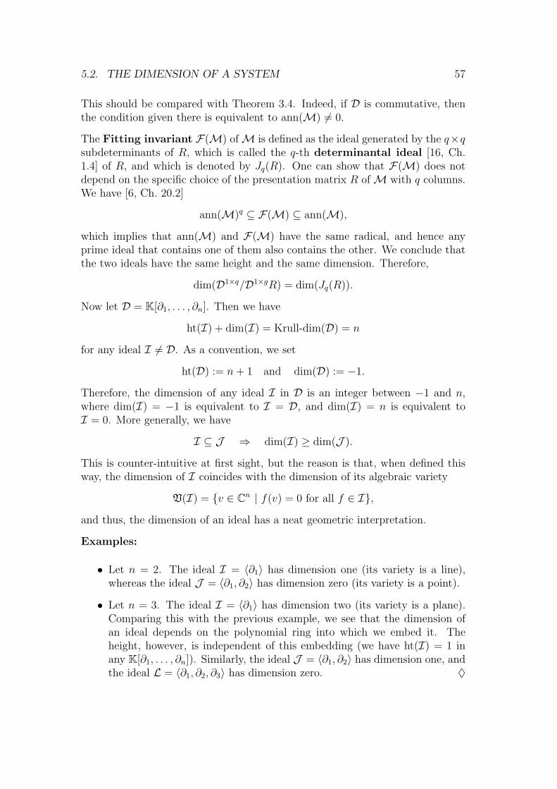
5.2. THE DIMENSION OF A SYSTEM 57

This should be compared with Theorem 3.4. Indeed, if D is commutative, thenthe condition given there is equivalent to ann(M) 6= 0.

The Fitting invariant F(M) ofM is defined as the ideal generated by the q×qsubdeterminants of R, which is called the q-th determinantal ideal [16, Ch.1.4] of R, and which is denoted by Jq(R). One can show that F(M) does notdepend on the specific choice of the presentation matrix R ofM with q columns.We have [6, Ch. 20.2]

ann(M)q ⊆ F(M) ⊆ ann(M),

which implies that ann(M) and F(M) have the same radical, and hence anyprime ideal that contains one of them also contains the other. We conclude thatthe two ideals have the same height and the same dimension. Therefore,

dim(D1×q/D1×gR) = dim(Jq(R)).

Now let D = K[∂1, . . . , ∂n]. Then we have

ht(I) + dim(I) = Krull-dim(D) = n

for any ideal I 6= D. As a convention, we set

ht(D) := n+ 1 and dim(D) := −1.

Therefore, the dimension of any ideal I in D is an integer between −1 and n,where dim(I) = −1 is equivalent to I = D, and dim(I) = n is equivalent toI = 0. More generally, we have

I ⊆ J ⇒ dim(I) ≥ dim(J ).

This is counter-intuitive at first sight, but the reason is that, when defined thisway, the dimension of I coincides with the dimension of its algebraic variety

V(I) = v ∈ Cn | f(v) = 0 for all f ∈ I,

and thus, the dimension of an ideal has a neat geometric interpretation.

Examples:

• Let n = 2. The ideal I = 〈∂1〉 has dimension one (its variety is a line),whereas the ideal J = 〈∂1, ∂2〉 has dimension zero (its variety is a point).

• Let n = 3. The ideal I = 〈∂1〉 has dimension two (its variety is a plane).Comparing this with the previous example, we see that the dimension ofan ideal depends on the polynomial ring into which we embed it. Theheight, however, is independent of this embedding (we have ht(I) = 1 inany K[∂1, . . . , ∂n]). Similarly, the ideal J = 〈∂1, ∂2〉 has dimension one, andthe ideal L = 〈∂1, ∂2, ∂3〉 has dimension zero. ♦


For D = K[∂1, . . . , ∂n], we also have the following characterization of the di-mension of an ideal I 6= D [1, Ch. 6.3]: Let J ⊆ 1, . . . , n and let DJ be thepolynomial ring (with coefficients in K) in the variables ∂j, j ∈ J . Clearly, DJ isa subring of D, and we put D∅ = K. Then

dim(I) = max|J | | I ∩ DJ = 0.

For example, dim(I) < 1 means that for all 1 ≤ i ≤ n, we have I ∩ K[∂i] 6= 0,that is, there exists 0 6= di ∈ I which depends only on the i-th variable.

Application to systems

Let B = w ∈ Aq | Rw = 0 and let M = D1×q/D1×gR. The dimension of Bis defined as the dimension of M. As outlined above, this is both equal to thedimension of the ideal ann(M) and equal to the dimension of Jq(R), which is theideal generated by the q × q minors of R.


1. dim(B) = −1.

2. B = 0.

Proof: We have B = 0 if and only if M = 0. However, M = 0 is equivalent toann(M) = D, which is true if and only if dim(B) = dim(ann(M)) = −1.


1. dim(B) < n.

2. B is autonomous.

Proof: We have dim(B) = n if and only if Jq(R) = 0. This means that all theq × q minors of R are zero, or equivalently, R does not have full column rank,which means that B is not autonomous.

Therefore, the dimension of a system B is always an integer between −1 and n,where dim(B) = −1 corresponds to B = 0, and dim(B) = n corresponds to Bhaving free variables. The dimensions between 0 and n− 1 yield a refinement ofthe concept of autonomy.

5.3. AUTONOMY DEGREES 59

5.3 Autonomy degrees

We say that B has autonomy degree at least r if

dim(B) < n− r.

Clearly, autonomy degree at least zero corresponds to autonomy itself. In whatfollows, we will give analytic interpretations of the autonomy degrees close to theextreme cases.

Autonomy degree at least n

The system B has autonomy degree at least n if and only if dim(B) < 0, whichmeans that B = 0, a very strong form of autonomy indeed.

Autonomy degree at least n− 1


1. B has autonomy degree at least n− 1.

2. B is finite-dimensional as a K-vector space.

Proof: We first observe that

ann(B) := d ∈ D | dB = 0 = ann(M).

To see this, recall that for any d ∈ ann(M), there exists X such that dI = XR,and thus Rw = 0 implies dw = 0. Conversely, if dw = 0 for all w ∈ B, we musthave dI = XR for some X, since MB(D1×gR) = D1×gR because of the injectivecogenerator property of A.

Now if dim(B) < 1, then ann(M) contains, for each 1 ≤ i ≤ n, an element0 6= di ∈ K[∂i]. Thus every component of w ∈ B satisfies n scalar ordinarydifferential equations (one for each independent variable). Since the solutionspaces of autonomous ordinary differential equations are finite-dimensional overKaccording to the lemma below, we obtain that B must be finite-dimensional as aK-vector space, too.

Conversely, let B be finite-dimensional over K, and let w1, . . . , wr be a K-basis.For each 1 ≤ i ≤ n and each 1 ≤ j ≤ r, consider the K-vector space spanned by


∂ki wj ∈ B, where k ∈ N. As a subspace of B, this space must be finite-dimensional,too. Thus there exists 0 6= dij ∈ K[∂i] such that dijwj = 0. But then we havediw = 0 for all w ∈ B for di := di1 · · · dir. This way, we can construct elements0 6= di ∈ ann(M) ∩K[∂i], showing that dim(ann(M)) < 1.

Lemma 5.9 Let n = 1. Then B is autonomous if and only if it is finite-dimensional as a K-vector space.

Proof: If B contains free variables, then it is certainly not finite-dimensionalover K, because the K-vector space A = C∞(R,K) has infinite dimension. Con-versely, if B is autonomous, then B ∼= y ∈ Ap | diyi = 0 for 1 ≤ i ≤ p forsome 0 6= di ∈ D, due to the Smith form. Each scalar ordinary differential equa-tion diyi = 0 has a solution space whose K-dimension equals the degree of di.Therefore B is also finite-dimensional over K.

For n ≥ 2 however, autonomy and finite K-dimension are no longer equivalent;autonomy is a weaker property. For example, B = w ∈ C∞(R2,K) | ∂1w = 0is autonomous, but not finite-dimensional (any smooth function depending onlyon the second variable belongs to B).

Examples:

• The system given by B = w ∈ A | grad(w) = 0 has the kernel represen-tation

R =

∂1...∂n

.Thus J1(R) = 〈∂1, . . . , ∂n〉 which has dimension zero for all n. Thereforeits solution space is finite-dimensional. Of course, this can also be seendirectly, because B consists of all constant functions in this example, andtherefore B ∼= K, which is a one-dimensional K-vector space.

• Let n = 2 and K = R. Consider B = w ∈ A | ∂21w = ∂2w, ∂

22w = w. Then

J1(R) = 〈∂21 − ∂2, ∂

22 − 1〉, which has dimension zero, because it contains

the elements ∂41 − 1 = (∂2

1 + ∂2)(∂21 − ∂2) + (∂2

2 − 1) and ∂22 − 1. If we

set x(t) := w(t1, t), considering t1 as a parameter, the equation ∂22w = w

becomes

x = x.

The solutions are of the form

x(t) = aet + be−t.

5.3. AUTONOMY DEGREES 61

Thusw(t1, t2) = a(t1)et2 + b(t1)e−t2 .

Now the equation ∂21w = ∂2w implies

a = a and b = −b,

and thus

a(t1) = c1et1 + c2e

−t1 and b(t1) = c3 cos(t1) + c4 sin(t1).

Finally, we have

w(t1, t2) = c1et1et2 + c2e

−t1et2 + c3 cos(t1)e−t2 + c4 sin(t1)e−t2 ,

showing that the solution space is four-dimensional over K = R. ♦

Remark: Systems with finiteK-dimension can be solved by iteratively solving or-dinary differential equations. Therefore, they behave very much like autonomousone-dimensional (n = 1) systems. For instance, they have only polynomial-exponential trajectories (with complex exponents admitted, which explains theappearance of sine and cosine in the previous example).

In fact, the K-vector space isomorphism M ∼= KN can be used to construct

pairwise commuting matrices Ai ∈ KN×N and a matrix C ∈ Kq×N such that

B = w ∈ Aq | ∃x ∈ AN : ∂ix = Aix for 1 ≤ i ≤ n and w = Cx

which can also be written as

B = w ∈ Aq | ∃x0 ∈ KN : w(t1, . . . , tn) = CeA1t1+...+Antnx0.

These are generalizations of one-dimensional autonomous systems, which afterreduction to first order, take the form x = Ax, w = Cx, or equivalently, w(t) =CeAtx0.

Autonomy degree at least 1

A system has autonomy degree at least one if and only if it is over-determined[18, Ch. 8]. This means that any smooth function v, defined on a neighborhoodof

U = x ∈ Rn | ‖x‖ ≥ r,where r > 0, and satisfying the local system law Rv = 0 there, can be uniquelyextended to an element w ∈ B, that is, there exists a unique w ∈ B (i.e., w isdefined on all of Rn and satisfies Rw = 0 everywhere) such that w(x) = v(x) forall x in a neighborhood of U .

We do not give the full proof, but only an overview of its main ingredients.


Theorem 5.10 1. If dim(B) < n − 1, then R is a right syzygy matrix, thatis, im(R) = ker(L) for some D-matrix L.

2. If

Dq R−→ Dg L−→ Dl

is exact, then so is

Aq0R−→ Ag0

L−→ Al0where A0 := C∞0 (Ω,K), and Ω = x ∈ Rn | ‖x‖ < r for some r > 0.

The space A0 consists of all smooth functions defined on Ω and having a compactsupport K ⊂ Ω. We identify

A0 = a ∈ A | supp(a) ⊂ Ω.

Let B have autonomy degree at least one. We show that B is over-determined.

The lemma above implies that R is a right syzygy matrix, say of L. Then thesequences of the theorem are both exact. Now let v as above be given. Since vis smooth on a neighborhood of U , there exists v ∈ Aq such that v(x) = v(x) forall x in a neighborhood of U . Since Rv = 0 on a neighborhood of U , we obtainthat Rv is zero in a neighborhood of U , that is, Rv ∈ Ag0 = C∞0 (Ω,K)g, where

Ω = x ∈ Rn | ‖x‖ < r = Rn \ U.

We need to construct w with Rw = 0 and w(x) = v(x) for all x in a neighborhoodof U . The theorem above implies that the inhomogeneous equation Rφ = Rvpossesses a solution φ ∈ Aq0 (because the right hand side is annihilated by L dueto LR = 0, and thus Rv ∈ kerA0(L) = imA0(R)). Thus we are finished by puttingw := v − φ. By construction, this w satisfies Rw = 0 and, since φ vanishes on aneighborhood of U , w coincides with v, and thus with v, on a neighborhood of U .This shows the existence of an extension w of v. Its uniqueness follows from theautonomy of B: If w1, w2 were two different extensions of v, then their differencewould be a non-zero compact support element of B. Lemma 5.1 shows that thisis impossible.

Examples:

• The system given by grad(w) = 0 is over-determined for all n ≥ 2.

• The Cauchy-Riemann equations for functions of one complex variable (cor-responding to n = 2 real variables) have the kernel representation

R =

[∂1 −∂2

∂2 ∂1

].

5.4. FREE SYSTEMS 63

We have J2(R) = 〈∂21 + ∂2

2〉 which has dimension one. Thus the result-ing system is autonomous, but not over-determined. Indeed, the functionf(z) = 1

zis analytic on any z ∈ C | |z| > ρ, where ρ > 0, and hence its

real and imaginary parts satisfy the Cauchy-Riemann equations. If f wereextendable to an analytic function on all of C, this would be a contradictionto the uniqueness of analytic continuation.

• The Cauchy-Riemann equation for functions of two complex (correspondingto n = 4 real) variables have the kernel representation

R =

∂1 −∂2

∂2 ∂1

∂3 −∂4

∂4 ∂3

.We have J2(R) = 〈∂2

1 + ∂22 , ∂1∂4 − ∂2∂3, ∂1∂3 + ∂2∂4, ∂

23 + ∂2

4〉 which hasdimension two. Thus the system is over-determined. ♦

Remark: Similarly as with autonomy, one can introduce controllability degrees[21, 22], but this is mathematically more involved. The lowest controllabilitydegree corresponds to controllability itself, and higher controllability degrees willgive various stronger versions of the controllability concept. In the next section,we study systems whose controllability degree is as large as possible, that is, aclass of systems with the strongest possible controllability properties.

5.4 Free systems

Controllability of B, that is, the existence of an image representation, amounts toM being torsion-free. A strong form of controllability is obtained whenM is evenfree (we will see below that this is equivalent to the existence of an observableimage representation). This property is called “strong controllability” of B bysome authors. However, since the term “strong controllability” is also used witha different meaning in the literature, it is preferable to speak of “free systems”(corresponding to the fact that the system module is free).

We say that B has an observable image representation if there exists L suchthat

B = w ∈ Aq | ∃!` ∈ Al : w = L`

that is, the latent variable ` is uniquely determined by the manifest variable w.In other words, ` is observable from w in the associated full system

Bf = [`T , wT ]T ∈ Al+q | L` = w.


This means that L must be left invertible. Thus we can conclude: B has anobservable image representation if and only if its kernel representation R is a leftsyzygy matrix of a left invertible matrix.


1. B possesses an observable image representation.

2. M is free, that is, M∼= D1×l for some l ∈ N. Equivalently, B ∼= Al.

Proof: If R is a left syzygy matrix of a left invertible matrix L, there is an exactsequence

D1×g ·R−→ D1×q ·L−→ D1×l −→ 0.

On the other hand, there is the exact sequence

D1×g ·R−→ D1×q−→M −→ 0.

From this, one can construct an isomorphism between M and D1×l as follows:Define φ : M → D1×l by φ([x]) := xL, where x ∈ D1×q and [x] is its residueclass in M. This is well-defined, because x = yR implies xL = yRL = 0. It isinjective, because conversely xL = 0 implies that x = yR for some y. Finally,the surjectivity of φ follows from the surjectivity of ·L.

Conversely, ifM is free, one can replaceM by someD1×l without losing exactnessin the sequence above. The resulting map from D1×q to D1×l can be identifiedwith ·L for some L ∈ Dq×l. Since ·L is surjective, the matrix L is left invertible.Thus R is a left syzygy matrix of a left invertible matrix.

Remark: The number l that appears in the second condition coincides with theinput-dimension of B. To see this, note that if

D1×g ·R−→ D1×q ·L−→ D1×l

is exact, then rank(R) + rank(L) = q. Similarly, if L is left invertible (that is,if ·L is surjective), we must have l = rank(L). Combining these equations, weobtain l = rank(L) = q − rank(R) = m, which is the input-dimension of B.

In Chapter 4, we have seen that controllability is also equivalent to B admitting aright invertible kernel representation. This equivalence does not hold in general,as can be seen from the system

B = w ∈ A3 | curl(w) = 0

discussed above: This system is controllable, but it cannot be represented by aright invertible matrix (or any matrix of full row rank). Still, the existence ofright invertible kernel representations is an interesting property also for multidi-mensional systems.


Theorem 5.12 (Quillen-Suslin) Let R ∈ Dg×q. The following are equivalent:

1. R is right invertible.

2. R can be embedded into a unimodular matrix, that is, there exists a D-matrix N such that [

RN

]∈ Dq×q

is unimodular.

Remark: This theorem has quite a remarkable history [11]: In 1955, J.-P. Serreraised the question whether projective modules over the polynomial ring D werefree. (A module is projective if it is a direct summand of a free module.) Someyears later, Serre himself was able to reduce the problem to the statement ofthe theorem above, but he did not succeed in proving it. Thus, the problembecame known as Serre’s conjecture. In 1976, it was solved by D. Quillen andA. Suslin, independently of each other, thus giving a positive answer to Serre’soriginal question.

Let R be a right invertible matrix, and let N be a matrix according to theQuillen-Suslin theorem. Set [

RN

]−1

=[X L

].

Then RX = I and NL = I, showing that L is left invertible. Moreover, RL = 0and XR + LN = I, implying that ker(·L) = im(·R). This shows that any rightinvertible matrix is a left syzygy matrix (and thus, any system represented bya right invertible matrix will be controllable), and moreover, it is a left syzygymatrix of a left invertible matrix.

Conversely, the transposed version of the Quillen-Suslin theorem (L is left invert-ible if and only if it can be embedded into a unimodular matrix [X,L]), shows thatany left invertible matrix possesses a left syzygy matrix that is right invertible.These considerations prove the following extension of the lemma above.


1. B admits a right invertible kernel representation.

2. B possesses an observable image representation.

3. M is free, that is, M∼= D1×l for some l ∈ N. Equivalently, B ∼= Al.


Control of free systems

Suppose that B is a free system, and let L, N be as above. Let w ∈ B. Then

w = L` ⇔ ` = Nw.

This can be used in order to compute connecting trajectories: Suppose thatw1, w2 ∈ B and U1, U2 are given. Compute `i = Nwi. Find a smooth function `that coincides with `1 on U1, and with `2 on U2. Then w = L` is a connectingtrajectory, i.e., it coincides with w1 on U1 and with w2 on U2. This procedure isknown as “flatness-based control”, and ` is called a “flat output” of the system.

Free systems are also very convenient for controller design. Let B be a givensystem, and let Bd ⊂ B be a subset containing certain desirable functions. Thetask is to design a controller C such that

B ∩ C = Bd and B + C = Aq.

The first requirement says that if the system laws Rw = 0 are additionallyconstrained by the controller laws Cw = 0, then the controlled system, whichis represented by [RT , CT ]T will only have desirable solutions. According to thefollowing lemma, the second statement is equivalent to rank(R) + rank(C) =rank[RT , CT ]T which means that the controller laws should be independent ofthe system laws (otherwise C = Bd would always be a trivial solution).

Lemma 5.14 Let Bi = w ∈ Aq | Riw = 0 for some Ri ∈ Dgi×q, where i = 1, 2.The following are equivalent:

1. B1 + B2 = Aq.

2. rank(R1) + rank(R2) = rank[RT1 , R

T2 ]T .

Proof: The input-dimension (idim) of Bi equals the dimension of kerK(Ri),where K is the quotient field of D, that is, the field of rational functions. Thus

idim(Bi) = q − rank(Ri).

If B1 + B2 = Aq, then we have

q = idim(Aq) = idim(B1 + B2) = idim(B1) + idim(B2)− idim(B1 ∩ B2)

= (q − rank(R1)) + (q − rank(R2))− (q − rank[RT1 , R

T2 ]T ).

This yields the desired result. Conversely, assume that assertion 2 is true. Weneed to show that B1 + B2 = Aq. By the fundamental principle, this is true if in


any left syzygy matrix [X, Y, Z] of

R :=

R1 00 R2

I I

the matrix Z must be zero. However, if [X, Y, Z] is a left syzygy matrix of R, thenXR1 = Y R2 = −Z. This means that the rows of Z belong to im(·R1)∩ im(·R2).However, this module is zero, because

rank[RT1 , R

T2 ]T = dim imK · [RT

1 , RT2 ]T = dim(imK(·R1) + imK(·R2))

= dim imK(·R1) + dim imK(·R2)− dim(imK(·R1) ∩ imK(·R2))

= rank(R1) + rank(R2)− dim(imK(·R1) ∩ imK(·R2))

yields dim(imK(·R1) ∩ imK(·R2)) = 0, which implies imK(·R1) ∩ imK(·R2) = 0,and thus im(·R1) ∩ im(·R2) = 0, since D ⊂ K.

Remark: Using the language of Chapter 2, we have B1 + B2 = Aq if and only if

M(B1) ∩M(B2) = M(B1 + B2) = M(Aq) = 0.

However, M(Bi) = im(·Ri), showing that B1 + B2 = Aq is equivalent to

im(·R1) ∩ im(·R2) = 0.

Then any equation of the form X1R1 +X2R2 = 0 implies that the summands areindividually zero, that is, XiRi = 0.

Theorem 5.15 B is a free system if and only if there exists B1 such that

B ⊕ B1 = Aq.

Proof: If B is free, it has a right invertible image representation. Let N be amatrix according to the Quillen-Suslin theorem, then B1 := w ∈ Aq | Nw = 0has the desired property.

Conversely, if B ⊕ B1 = Aq for some B1 = w ∈ Aq | Nw = 0, then the matrix[RN

]has a left inverse, say [X,L] (this follows from B ∩ B1 = 0), and the rank of[RT , NT ]T equals rank(R) + rank(N) (this follows from B + B1 = Aq). Theequation XR + LN = I yields (RX − I)R + RLN = 0, and hence, by the


previous remark, we must have RXR = R. Then we have, for the system moduleM = D1×q/D1×gR, an isomorphism

D1×q ∼=M⊕D1×gR, x 7→ ([x], xXR).

The surjectivity of this map follows from

D1×gR = D1×gRXR ⊆ D1×qXR ⊆ D1×gR

which implies that these modules are actually equal. For injectivity, suppose that[x] = 0 and xXR = 0. Then x = yR for some y, and 0 = yRXR = yR, whichyields x = 0. This isomorphism shows that M is a direct summand of a freeD-module, that is, M is projective. As remarked above, it is a consequence ofthe Quillen-Suslin theorem that projective D-modules are free.

Remark: The “only if” direction could also be proved without using the Quillen-Suslin theorem. Indeed, ifM is free, then it is also projective. This is equivalentto the existence of X with RXR = R (similarly as in the proof of the “if”direction). Then

kerA(R)⊕ imA(XR) = Aq

and thus we may put B1 := imA(XR).

Using the complementary system B1, the controller design problem for a freesystem B can easily be solved by putting

C = B1 + Bd.

ThenB + C = B + B1 + Bd = Aq

andB ∩ C = B ∩ (B1 + Bd) = (B ∩ B1) + Bd = Bd

where we have used the modular law

Bd ⊆ B ⇒ B ∩ (B1 + Bd) = (B ∩ B1) + Bd.

Appendix A

Background material

A.1 Kalman controllability criterion

In this section, we prove Theorem 1.2.

Let A ∈ Rn×n and B ∈ Rn×m. Let U be such that

C0(R,R)m ⊇ U ⊇ O(R,R)m,

where C0 denotes the continuous functions and O denotes the analytic functions.

Then x = Ax+Bu, x(0) = x0 has the unique solution

x(t) = eAtx0 +

∫ t

0

eA(t−τ)Bu(τ)dτ.

Lemma A.1.1 (Identity theorem for analytic functions) Let f :R→R1×m

be an analytic function. Then

f ≡ 0 ⇔ f (i)(0) = 0 for all i ∈ N.

Lemma A.1.2 All powers Ai of A, where i ∈ N, are R-linear combinations ofA0 = I, A1 = A, . . . , An−1.

Proof: This follows from the Hamilton-Cayley theorem: χA(A) = 0, where χAis the characteristic polynomial of A, a polynomial of degree n.

Lemma A.1.3 Let t > 0 and

K := [B,AB, . . . , An−1B] and Wt :=

∫ t

0

eAτBBT eAT τdτ.

Then rank(K) = rank(Wt).

69

70 APPENDIX A. BACKGROUND MATERIAL

In particular, the following are equivalent:

1. rank(K) = n.

2. Wt is non-singular.

Proof: Let t > 0 and ξ ∈ R1×n. Note that Wt is symmetric and positive semi-definite. Hence we have ξWt = 0 ⇔ ξWtξ

T = 0 ⇔∫ t

0

‖ξeAτB‖2dτ = 0

⇔ f ≡ 0, where f(t) = ξeAtB ⇔ f (i)(0) = ξAiB = 0 for all i ∈ N ⇔ξK = 0. Thus ker(·Wt) = ker(·K), and thus dim(ker(·Wt)) = n − rank(Wt) =dim(ker(·K)) = n− rank(K).

Theorem A.1.4 The following are equivalent:

1. ∃t1 > 0 ∀x0, x1 ∈ Rn: x0 can be controlled to x1 in time t1, that is, ∃u ∈ U

such that the solution to

x = Ax+Bu, x(0) = x0

satisfies x(t1) = x1.

2. rank(K) = n, where K = [B,AB, . . . , An−1B].

Proof: 1⇒ 2: Assume that rank(K) < n. Then there exists 0 6= ξ ∈ R1×n suchthat ξK = 0. This means that ξAiB = 0 for 0 ≤ i ≤ n − 1. According to thelemma, this implies

ξAiB = 0 for all i ∈ N.

Consider the analytic function f(t) = ξeAtB. We have f (i)(0) = 0 for all i ∈ Nand hence f ≡ 0.

If x0 = 0 can be controlled to x1 in time t1, then

x1 =

∫ t1

0

eA(t1−τ)Bu(τ)dτ

and then ξx1 = 0. Since this does not hold for all x1, assertion 1 is not true.

2⇒ 1: Let rank(K) = n. Let x0, x1 be given. Let t1 > 0 be arbitrary. Set

u(t) = BT eAT (t1−t)W−1

t1(x1 − eAt1x0).

A.1. KALMAN CONTROLLABILITY CRITERION 71

This is an analytic function and hence it belongs to U. The solution of x =Ax+Bu satisfies

x(t1) = eAt1x0 +

∫ t1

0

eA(t1−τ)BBT eAT (t1−τ)dτW−1

t1(x1 − eAt1x0)

= eAt1x0 +Wt1W−1t1

(x1 − eAt1x0)

= x1

and hence we have the desired result.

In fact, the proof shows more than originally claimed: rank(K) = n is equivalentto the following stronger version of assertion 1:

∀t1 > 0 and ∀x0, x1 there exists u ∈ U such that the solution to x = Ax + Bu,x(0) = x0 satisfies x(t1) = x1.

In other words, if x0 can be controlled to x1 at all, then this can be done inan arbitrarily small time t1 > 0. This feature, which has no analogue in discretetime, is counter-intuitive at first sight: In a “real world” system, it certainly takes“some time” to change from one state to another. The reason is that we admitarbitrarily large input values here, i.e., we make the optimistic assumption thatwe can put as much “energy” as we like into the system. In a real world system,there are constraints which limit the size of the admissible inputs, and this hasthe consequence that the transition from one state to another cannot be donearbitrarily fast in practice.

Theorem A.1.5 Let x = Ax+Bu be controllable, and let u be an input functionthat controls x = Ax+Bu from x(0) = 0 to x(t1) = x1, where t1 > 0. Then

E(u) :=

∫ t1

0

‖u(t)‖2dt ≥ Emin(t1, x1) := xT1W−1t1x1

and equality is achieved for the input function

u(t) = BT eAT (t1−t)W−1

t1x1. (A.1)

In other words, the input function from (A.1) is optimal in the sense that itsenergy E(u) is minimal among the energies of all u that steer the system fromx(0) = 0 to x(t1) = x1. This minimal energy is given by Emin(t1, x1) = xT1W

−1t1 x1.

This shows that the smaller t1 is, the more energy is needed to do the transitionfrom 0 to x1 in time t1. More precisely, if 0 < s < t, then Wt > Ws (this notationmeans that Wt−Ws is positive definite), which implies, using some linear algebra,W−1s > W−1

t , and hence

Emin(s, x) = xTW−1s x > xTW−1

t x = Emin(t, x) for all x 6= 0.


This explains the trade-off between the speed of control on the one hand and theenergy consumption of control on the other.

Proof: DefineV (t, x) := xTW−1

t x.

Let us look at the change of V (t, x(t)) along a trajectory x of our system. Wehave

ddtV (t, x(t)) = d

dtx(t)TW−1

t x(t)

= x(t)TW−1t x(t) + x(t)T ( d

dtW−1t )x(t) + x(t)TW−1

t x(t).

Note that for any matrix-valued function W ,

ddtW−1t = −W−1

t WtW−1t .

Moreover, we plug in x = Ax + Bu and we obtain (omitting the argument t inx(t) and u(t) for simplicity)

ddtV (t, x) = (Ax+Bu)TW−1

t x− xTW−1t WtW

−1t x+ xTW−1

t (Ax+Bu)

= xT (ATW−1t +W−1

t A−W−1t WtW

−1t )x+ 2uTBTW−1

t x.

Consider the matrix

Xt := ATW−1t +W−1

t A−W−1t WtW

−1t .

We have

WtXtWt = WtAT + AWt − Wt (A.2)

=

∫ t

0

(eAτBBT eAT τAT + AeAτBBT eA

T τ )dτ − Wt

= eAτBBT eAT τ∣∣∣τ=t

τ=0− Wt

= eAtBBT eAT t −BBT − Wt.

Noting that by the definition of W ,

Wt = eAtBBT eAT t

we obtainWtXtWt = −BBT (A.3)

and hence Xt = −W−1t BBTW−1

t . We use this to rewrite our expression forddtV (t, x) and obtain

ddtV (t, x) = −xTW−1

t BBTW−1t x+ 2uTBTW−1

t x

= −‖BTW−1t x‖2 + 2〈u,BTW−1

t x〉= ‖u‖2 − ‖u−BTW−1

t x‖2.

A.1. KALMAN CONTROLLABILITY CRITERION 73

Let’s integrate this from 0 to t1, exploiting that x(0) = 0 and x(t1) = x1. Then

V (t1, x1)− V (0, 0) =

∫ t1

0

‖u(t)‖2dt−∫ t1

0

‖u(t)−BTW−1t x(t)‖2dt

or

xT1W−1t1x1 = E(u)−

∫ t1

0

‖u(t)−BTW−1t x(t)‖2dt ≤ E(u). (A.4)

This shows that

E(u) ≥ Emin(t1, x1) := xT1W−1t1x1.

Equality is achieved if and only if the integral in (A.4) vanishes, i.e., if

u(t) = BTW−1t x(t). (A.5)

Plugging that into x = Ax+Bu, we get

x(t) = (A+BBTW−1t )x(t).

Since we know that x(t1) = x1, the solution of this linear time-varying ODE isuniquely determined for all t > 0. This solution is given by

ξ(t) = WteAT (t1−t)W−1

t1x1.

This can easily be checked: We have ξ(t1) = x1 and

ξ(t) = (Wt −WtAT )eA

T (t1−t)W−1t1x1.

Combining (A.2) with (A.3), we see that

Wt = WtAT + AWt +BBT .

This implies

ξ(t) = (AWt +BBT )eAT (t1−t)W−1

t1x1

= (A+BBTW−1t )Wte

AT (t1−t)W−1t1x1

= (A+BBTW−1t )ξ(t)

as desired. Thus x = ξ is the optimal state trajectory. Then, according to (A.5),

u(t) = BTW−1t ξ(t) = BT eA

T (t1−t)W−1t1x1

is the minimum energy control function that steers the system from 0 to x1 intime t1.


A.2 Galois correspondences

A partial order on a set X is a relation ≤ with the properties:

• x ≤ x (reflexivity);

• x1 ≤ x2 and x2 ≤ x3 ⇒ x1 ≤ x3 (transitivity);

• x1 ≤ x2 and x2 ≤ x1 ⇒ x1 = x2 (antisymmetry).

The term “partial” refers to the fact that there may be elements x1, x2 ∈ X suchthat neither x1 ≤ x2 nor x2 ≤ x1 is true.

Let X and Y be partially ordered sets and let f : X → Y and g : Y → X be twomaps. The mappings f and g are called a Galois correspondence if

1. f and g are order-reversing, that is,

x1 ≤ x2 ⇒ f(x1) ≥ f(x2) and y1 ≤ y2 ⇒ g(y1) ≥ g(y2);

2. x ≤ g(f(x)) for all x ∈ X and y ≤ f(g(y)) for all y ∈ Y .

Lemma A.2.1 We have gfg ≡ g and fgf ≡ f . Thus there are order-reversingbijections

im(g) ↔ im(f)

x → f(x)

g(y) ← y

that are inverse to each other.

Proof: Due to property 2, we have f(g(y)) ≥ y and g(f(g(y))) ≥ g(y). Applyingthe order-reversing mapping g to the first inequality, we obtain g(f(g(y)) ≤ g(y).Combining these inequalities, we obtain g(f(g(y))) = g(y). Since this holds forall y ∈ Y , we have gfg ≡ g. The second statement is analogous.

We show that the map f1 : im(g) → im(f), x 7→ f(x) is a bijection. Forinjectivity, let f(x1) = f(x2) for some x1, x2 ∈ im(g), that is, xi = g(yi) for somey1, y2 ∈ Y . Thus

f(g(y1)) = f(g(y2)).

Applying g and using gfg ≡ g, we obtain

x1 = g(y1) = g(f(g(y1))) = g(f(g(y2))) = g(y2) = x2.

A.2. GALOIS CORRESPONDENCES 75

Secondly, we show that f1 is surjective: Let y ∈ im(f) be given, that is, y = f(x)for some x ∈ X. Using fgf ≡ f , we have y = f(x) = f(g(f(x))) and thus, withx := g(f(x)) ∈ im(g), we have y = f(x).

Similarly, one shows that g1 : im(f)→ im(g), y 7→ g(y) is a bijection.

It remains to be shown that f1 and g1 are inverse to each other: However, wehave, for x = g(y): g(f(x)) = g(f(g(y))) = g(y) = x and similarly, the other wayround.

Define x := gf(x) for all x ∈ X. Then

• x ≤ x = gf(x);

• x = gfgf(x) = gf(x) = x;

• if x1 ≤ x2, then f(x1) ≥ f(x2), and thus x1 = gf(x1) ≤ gf(x2) = x2.

This shows that gf is a closure operation. We say that x is closed if x = x.This is true if and only if x ∈ im(g). Analogous statements can be shown if weset y := fg(y) for all y ∈ Y .

Note that if only the left hand side X of the Galois correspondence is restrictedto im(g) ⊆ X, we have order-reversing maps

im(g) → Y

x → f(x)

g(y) ← y

with

x = g(f(x)) = x for all x ∈ im(g)

and

y = f(g(y)) ≥ y for all y ∈ Y.

This was used in Chapter 2 for X = A, Y = M, f ≡M, g ≡ B. Then im(g) = B.The partial order is given by inclusion.

Here are two other prominent examples of Galois correspondences, where thepartial order is also given by inclusion:

• Let X be the set of all subsets of Cn and let Y be the set of all ideals inK[s1, . . . , sn]. Let f ≡ I be defined by

I(V ) = f ∈ K[s1, . . . , sn] | f(v) = 0 for all v ∈ V


and let g ≡ V be defined by

V(I) = v ∈ Cn | f(v) = 0 for all f ∈ I.

Then VI(V ) ⊇ V is called the Zariski closure of V , and V is called analgebraic variety if it is Zariski closed. Thus im(V) is the set of all algebraicvarieties, and IV(I) = Rad(I) := f ∈ K[s1, . . . , sn] | ∃l ∈ N : f l ∈ Iby Hilbert’s Nullstellensatz. The ideal Rad(I) ⊇ I is the closure of I withrespect to this correspondence.

• Let X = Y be the set of all subspaces of Rn, and let f = g be defined byf(V ) = V ⊥, the orthogonal complement of V with respect to the standardscalar product 〈x, y〉 = xTy. In this case the Galois correspondence consistsalready of order-reversing bijections inverse to each other.

A lattice is a partially ordered set X in which any two elements x1, x2 ∈ Xpossess an infimum x1 ∧ x2 ∈ X and a supremum x1 ∨ x2 ∈ X, that is

• x1 ∧ x2 ≤ xi for i = 1, 2; and x ≤ xi for i = 1, 2 implies x ≤ x1 ∧ x2;

• x1 ∨ x2 ≥ xi for i = 1, 2; and x ≥ xi for i = 1, 2 implies x ≥ x1 ∨ x2.

For example, let X be the power set of a given set. This is partially ordered byinclusion, and it becomes a lattice by taking the union as the supremum, and theintersection as the infimum.

Similarly, the set X of all subspaces of a given vector space is partially orderedby inclusion, and we take the sum as the supremum, and the intersection as theinfimum.

The set M of all left D-submodules of D1×q becomes a lattice in the same way.

Note that the set B of all abstract linear systems becomes a lattice if we canshow that it is closed under addition.

Let X, Y be two lattices and let f : X → Y be an order-reversing bijection withorder-reversing inverse. Then we call f a lattice anti-isomorphism and we have

f(x1 ∧ x2) = f(x1) ∨ f(x2)

f(x1 ∨ x2) = f(x1) ∧ f(x2)

for all x1, x2 ∈ X.

A.3. PROPERTY O FOR 1-D TIME-INVARIANT SYSTEMS 77

A.3 Property O for 1-d time-invariant systems


The commutative ring D = K[ ddt

] is a Euclidean domain, that is, we have a“division with remainder”: For all 0 6= d ∈ D and all n ∈ D, there exist q, r ∈ Dsuch that n = qd+ r, where the “remainder” r satisfies either r = 0 or deg(r) <deg(d). It is known that Euclidean domains are principal ideal domains, that is,every ideal in D can be generated by one single element. A matrix U ∈ K[s]g×g iscalled unimodular if there exists U−1 ∈ K[s]g×g. Equivalently, det(U) ∈ K\0.

Lemma A.3.1 (Smith form) For every R ∈ K[s]g×q, there exist unimodularmatrices U ∈ K[s]g×g and V ∈ K[s]q×q such that

URV =

[D 00 0

]where D = diag(d1, . . . , dp) for some 0 6= di ∈ K[s] and d1|d2| . . . |dp. Here,p = rank(R).

Moreover, since D is Euclidean, the unimodular transformation matrices U and Vcan be obtained by performing elementary row and column operations. By anelementary operation, we mean one of the following matrix transformations:

• interchanging two rows (columns) of a matrix;

• adding a multiple of one row (column) to another row (column);

• multiplying a row (column) by a unit, that is, an element of K \ 0.

It is easy to see that these operations correspond to multiplication by unimodularmatrices from the left and right.

Proof: Without loss of generality, let R 6= 0. It is sufficient to show that byelementary operations, R can be brought into the form

R′ =

a 0 · · · 00... Q0

(A.6)

where a divides all entries of Q. Then one applies the same procedure to Q, andthe result follows inductively.


Case 1: There exists i, j such that Rij divides all entries of R. By a suitableinterchange of rows and columns, this element can be brought into the (1,1)position of the matrix. Therefore without loss of generality, R11 divides all entriesof R. Now perform the following elementary operations: for all i 6= 1, put ithrow minus Ri1/R11 times 1st row; for all j 6= 1, put jth column minus R1j/R11

times 1st column. Then we are finished.

Case 2: There is no i, j such that Rij divides all entries of R. Let

δ(R) := mindeg(Rij) | Rij 6= 0.

Without loss of generality, deg(R11) = δ(R). We show that by elementary op-erations, we can transform R into R(1) with δ(R(1)) < δ(R). Then we obtain astrictly decreasing sequence δ(R) > δ(R(1)) > δ(R(2)) > . . . ≥ 0. After finitelymany steps, we arrive at zero, i.e., we obtain a matrix which has a unit as anentry, and thus we are in Case 1.

Case 2a: R11 does not divide all R1j, Ri1, say, it does not divide R1k. By theEuclidean algorithm, we can write

R1k = R11q + r

where r 6= 0 and deg(r) < deg(R11). Perform the elementary operation: kthcolumn minus q times 1st column. Then the new matrix R(1) has r in the (1, k)position and thus δ(R(1)) < δ(R) as desired.

Case 2b: R11 divides all R1j, Ri1. Similarly as in Case 1, we can transform,by elementary operations, R into the form (A.6). If a divides all entries of Q,then we are finished. If there exists i, j such that a does not divide Qij, thenwe perform the elementary operation: 1st row plus (i+ 1)st row. (Note that the(i+ 1)st row of R′ corresponds to the ith row of Q.) The new matrix has Qij inthe (1, j + 1) position and therefore we are in Case 2a.

Theorem A.3.2 Let D = K[ ddt

] and let A consist of all polynomial-exponentialfunctions. Then A has property O.

Proof: We need to show that M = MB(M) for all M = D1×gR for someR ∈ Dg×q. Due to the Smith form, it suffices to consider the case where g = q = 1.

Thus let R ∈ D. If R = 0, then M = 0 and B(M) = A. The only linear constant-coefficient ordinary differential equation which has all a ∈ A as solutions is thetrivial equation. Therefore, MB(M) = 0 = M . If R is a non-zero constant, thenM = D and B(M) = 0 and thus MB(M) = D = M .

A.4. LEFT-EXACTNESS OF THE HOM-FUNCTOR 79

Let us assume that R is not constant, and let M = DR. By the fundamentaltheorem of algebra, there exists a representation

R = ck∏i=1

( ddt− λi)µi (A.7)

where c ∈ K, k and µi are positive integers, and λi ∈ C. From the theory of linearconstant-coefficient ordinary differential equations, it is known that B = B(M)consists of all functions of the form

w(t) =k∑i=1

pi(t)eλit

where pi ∈ C[t] is an arbitrary polynomial of degree µi − 1. On the other hand,the only elements of D that annihilate all these w are the multiples of R. HenceM(B) = MB(M) = DR = M .

The discrete counterpart given in Theorem 2.7 is proven similarly (using theSmith form and some basic facts about the solutions of linear constant-coefficientdifference equations). However, the proof of the multivariate versions, that is,Theorems 2.9 and 2.10, is much harder, because D = K[∂1, . . . , ∂n] is not aprincipal ideal domain, and therefore there exists no analogue of the Smith form,for n ≥ 2.

A.4 Left-exactness of the Hom-functor

In this section, we prove Lemma 2.14, which is restated below.

Let D be a ring, and let A be a left D-module. For a left D-module M, we set

HomD(M,A) = φ :M→A | φ is D-linear.

If N is another left D-module, and if f :M→N is a D-linear map, then

HomD(f,A) : HomD(N ,A)→ HomD(M,A), ψ 7→ ψ f.

Lemma A.4.1 The functor HomD(·,A) is left exact, that is, if

M f−→ N g−→ P −→ 0

is exact, where M,N ,P are left D-modules, and f, g are D-linear maps, then

HomD(M,A)HomD(f,A)←− HomD(N ,A)

HomD(g,A)←− HomD(P ,A)←− 0

is also exact.


Proof: We first show that HomD(g,A) is injective. Suppose that HomD(g,A)ϕ =ϕ g = 0 for some ϕ ∈ HomD(P ,A). This means that ϕ(g(n)) = 0 for all n ∈ N .Since g is surjective, this implies ϕ(p) = 0 for all p ∈ P , and thus ϕ = 0.

Secondly, we have that HomD(f,A) HomD(g,A) = HomD(g f,A) = 0, sinceg f = 0. Therefore ker(HomD(f,A)) ⊇ im(HomD(g,A)).

Finally, we prove that ker(HomD(f,A)) ⊆ im(HomD(g,A)). For this, let ψ ∈HomD(N ,A) be such that ψ f = 0. We need to show that ψ = ϕ g forsome ϕ ∈ HomD(P ,A). Let p ∈ P be given. Since g is surjective, there existsn ∈ N such that g(n) = p. We put ϕ(p) := ψ(n). This is well-defined, becauseg(n1) = g(n2) = p implies n1 − n2 ∈ ker(g) = im(f) and hence ψ(n1) = ψ(n2).The map ϕ satisfies ϕ(g(n)) = ψ(n) for all n ∈ N , and thus ψ = ϕ g as desired.To see that ϕ is D-linear, let p1, p2 ∈ P and d1, d2 ∈ D. Note that g(ni) = pi fori = 1, 2 implies g(d1n1 + d2n2) = d1p1 + d2p2 and thus

ϕ(d1p1 + d2p2) = ψ(d1n1 + d2n2) = d1ψ(n1) + d2ψ(n2) = d1ϕ(p1) + d2ϕ(p2),

where we have used the linearity of g and ψ.

A.5 Baer’s criterion

In this section, we prove the alternative version of Baer’s criterion which doesnot rely on the axiom of choice; see e.g. [12, Ch. 1, §3] for the classical version.

T = HomD(·,A) is an exact functor on the category of left D-modules if, forevery exact sequence

M f−→ N g−→ P

of left D-modules, the sequence

TM Tf←− TN Tg←− TP

is also exact. This is equivalent to saying that A is injective.

Lemma A.5.1 T = HomD(·,A) is exact if and only if it turns every exact se-quence of the form

0→ N → P

into an exact sequence

0← TN ← TP .

A.5. BAER’S CRITERION 81

Proof: The condition is clearly necessary. For sufficiency, let

M f−→ N g−→ P

be a given exact sequence. Consider

M f−→ N g1−→ im(g) −→ 0.

Using the fact that the Hom-functor is left exact, this yields an exact sequence

TM← TN ← T im(g)← 0.

We need to show that


is exact, that is, for ϕ ∈ HomD(N ,A), we have to prove that

ϕ f = 0 ⇔ ∃ψ ∈ HomD(P ,A) : ϕ = ψ g.

The implication “⇐” is trivial, because g f = 0. For “⇒”, note that ϕ f = 0implies that there exists θ ∈ HomD(im(g),A) such that ϕ = θ g1. However,

0→ im(g) → P

is exact, and therefore, using the assumption,

0← HomD(im(g),A)← HomD(P ,A)

is also exact, which means that θ can be extended to a map ψ ∈ HomD(P ,A),that is, ψ|im(g) = θ. Therefore ϕ = θ g1 = θ g = ψ g.

Now let D be left Noetherian, and consider T as a functor on the category offinitely generated left D-modules, that is, T is exact if it turns every exact se-quence of finitely generated left D-modules into an exact sequence.

Theorem A.5.2 T = HomD(·,A) is exact if and only if for every sequence

0→ I → D,

where I is a left ideal in D, the sequence


is also exact.


Proof: The condition is clearly necessary. For sufficiency, let

0→ N → P

be a given exact sequence. We need to show that 0← TN ← TP is exact, thatis, for ϕ ∈ HomD(N ,A), we have to prove that there exists ψ ∈ HomD(P ,A)such that ϕ = ψ|N . Let ϕ be given.

Consider the set of all submodules N ⊆ Q ⊆ P with the property that thereexists ψ ∈ HomD(Q,A) with ϕ = ψ|N . Since D is left Noetherian, this non-empty family of left submodules of the finitely generated module P possesses amaximal element, say Q1. Let ψ1 ∈ HomD(Q1,A) be such that ϕ = ψ1|N . Weare finished if we can show that P ⊆ Q1.

Assume conversely that x ∈ P \ Q1. Set

I := d ∈ D | dx ∈ Q1.

This is a left ideal in D. Define φ ∈ HomD(I,A) via

φ(d) := ψ1(dx).

By assumption, there exists θ ∈ HomD(D,A) such that θ|I = φ. The map θ isuniquely determined be a := θ(1) ∈ A, via θ(d) = dθ(1) = da, and thus

φ(d) = da

for all d ∈ I. Now let Q2 := Q1 +Dx. Since x /∈ Q1, this is a proper supermoduleof Q1. Set

ψ2(q2) := ψ2(q1 + dx) := ψ1(q1) + da.

To see that this is well-defined, let q2 = q1+dx = q′1+d′x. Then q1−q′1 = (d′−d)x,and thus d′− d ∈ I. Hence φ(d′− d) = (d′− d)a. On the other hand, φ(d′− d) =ψ1((d′ − d)x) = ψ1(q1 − q′1) = ψ1(q1)− ψ1(q′1). Thus ψ1(q1) + da = ψ1(q′1) + d′a.

Moreover, ψ2 is D-linear, because

ψ2(q2 + q′2) = ψ2(q1 + q′1 + dx+ d′x) = ψ1(q1 + q′1) + (d+ d′)a

= ψ1(q1) + da+ ψ1(q′1) + d′a = ψ2(q2) + ψ2(q′2)

and

ψ2(d′q2) = ψ2(d′q1 + d′dx) = ψ1(d′q1) + d′da = d′ψ1(q1) + d′da = d′ψ2(q2).

Finally, we show that ψ2|N = ϕ: Since N ⊆ Q1, we have

ψ2(n) = ψ1(n) = ϕ(n)

for all n ∈ N . Thus we have a contradiction to the maximality of Q1.

A.6. CRITERION FOR THE COGENERATOR PROPERTY 83

A.6 Criterion for the cogenerator property


First, we recall the definition of a (co-)generator [10, p. 53]. Let D be a ring(with unity), and let A be a left D-module. One calls A a generator if for allleft D-modules N , one has

N =∑

ϕ∈HomD(A,N )

im(ϕ)

and A is said to be a cogenerator if for all left D-modules N , we have

0 =⋂

ϕ∈HomD(N ,A)

ker(ϕ).

Lemma A.6.1 The following are equivalent:

1. A is a cogenerator.

2. If HomD(f,A) = 0, then f = 0.

In the second assertion, f : M → N is an arbitrary D-linear map between twoarbitrary left D-modules M,N .

Proof: “1⇒ 2”: Assume conversely that f :M→N is not identically zero, thatis, f(m0) 6= 0 for some m0 ∈M, but HomD(f,A) = 0, that is, ϕf = 0 for all ϕ ∈HomD(N ,A). This means that ϕ(f(m0)) = 0 for all ϕ ∈ HomD(N ,A), and hencef(m0) 6= 0 is contained in the intersection of all kernels of ϕ ∈ HomD(N ,A).

“2 ⇒ 1”: Let N be such that there exists 0 6= n0 ∈ N with n0 ∈ ker(ϕ) for allϕ ∈ HomD(N ,A). Consider the map f : D → N defined by f(1) = n0, thatis, f(d) = dn0 for all d ∈ D. Then f is not identically zero, but HomD(f,A) is,because

ϕ(f(d)) = ϕ(dn0) = dϕ(n0) = 0

for all d ∈ D, and hence ϕ f = 0 for all ϕ ∈ HomD(N ,A).

In the following, we will see that if A is injective (which means that the functorHomD(·,A) is exact, i.e., it preserves exactness), then the cogenerator propertyis equivalent to saying that the functor HomD(·,A) is faithful (i.e., it reflectsexactness).

Let T be a contravariant additive functor from the left D-modules to the (ad-ditive) Abelian groups, that is, T assigns to each left D-module M an Abeliangroup TM, and to each D-linear map f : M → N a group homomorphismTf : TN → TM with


1. T idM = idTM;

2. T (g f) = Tf Tg;

3. T (f + g) = Tf + Tg;

4. If f = 0, then Tf = 0.

Note that conditions 1 and 4 imply: If M = 0, then TM = 0.

A typical example for such a functor is T = HomD(·,A). Additionally, assumethat T is exact, that is, if

M f−→ N g−→ P

is exact, then so is

TM Tf←− TN Tg←− TP .

For T = HomD(·,A), exactness means injectivity of A.


1. If TM = 0, then M = 0.

2. If Tf = 0, then f = 0.

For T = HomD(·,A), this means that A is a cogenerator.

Proof: “2 ⇒ 1”: Let M 6= 0. Then idM 6= 0. By assertion 2, T idM 6= 0. SinceT idM = idTM, it follows that TM 6= 0.

“1⇒ 2”: Let f :M→ N be given. We have f = i f1, where f1 :M→ im(f)and i : im(f) → N . Then Tf = Tf1 Ti. Suppose that Tf = 0. Sincef1 is surjective, Tf1 is injective. Thus Ti = 0. On the other hand, since i isinjective, Ti is surjective. Thus im(Ti) = T im(f) = 0. Using assertion 1, wehave im(f) = 0, that is, f = 0.

Theorem A.6.3 The following are equivalent:

1. If TM = 0, then M = 0.

2. If TM← TN ← TP is exact, then so is M→N → P.

If the second assertion is true, one says that T is faithful, or that T reflectsexactness. Again, for T = HomD(·,A), this means that A is a cogenerator.

A.6. CRITERION FOR THE COGENERATOR PROPERTY 85

Proof: “2 ⇒ 1”: Let TM = 0. Then 0 ← TM ← 0 is exact. By assertion 2,0→M→ 0 is exact, which means that M = 0.

“1⇒ 2”: Let

M f−→ N g−→ P

be not exact. We need to show that


is not exact.

Case 1: g f 6= 0. Then, using the lemma, T (g f) 6= 0, that is, Tf Tg 6= 0,and we’re finished.

Case 2: g f = 0, that is, im(f) ( ker(g). Then T (g f) = Tf Tg = 0, that isim(Tg) ⊆ ker(Tf). We need to show that this inclusion is strict. Define

σ : ker(g) → N and π : N → N /im(f).

Then

ker(g)σ−→ N g−→ P and M f−→ N π−→ N /im(f)

are both exact. Therefore

T ker(g)Tσ←− TN Tg←− TP and TM Tf←− TN Tπ←− T (N /im(f))

are also exact. Thus

ker(Tσ) = im(Tg) ⊆ ker(Tf) = im(Tπ).

The fact that im(f) ( ker(g) means that π σ 6= 0, and hence Tσ Tπ 6= 0. Thisshows that the above inclusion must be strict.

Corollary A.6.4 Let T = HomD(·,A) with A injective. The following are equiv-alent:

1. If TM = 0, then M = 0.

2. If TM = 0 and M is finitely generated, then M = 0.

3. If TM = 0 and M is generated by one single element, then M = 0.



Proof: The equivalence of assertions 1 and 4 was shown in a lemma above. Since“1 ⇒ 2 ⇒ 3” is obvious, it suffices to show “3 ⇒ 1”. Let M 6= 0. We need toshow that HomD(M,A) 6= 0, that is, there exists a non-zero D-linear map fromM to A. Let 0 6= m ∈M. Then 0 6= Dm ⊆M and there is an exact sequence

0→ Dm →M.

Since A is injective, the sequence

0← HomD(Dm,A)← HomD(M,A)

is also exact, and by condition 3, HomD(Dm,A) 6= 0, that is, there exists a non-zero D-linear map ψ : Dm → A. However, the exactness of the last sequencesays that there exists a D-linear map φ :M→A with φ|Dm = ψ. Thus φ 6= 0.

If D is left Noetherian, we can proceed analogously with the category of finitelygenerated left D-modules. (Note that we need the Noetherian property to guar-antee that kernels and images of D-linear maps between finitely generated D-modules are again finitely generated.) Then we obtain the following alternativeversion of Theorem 2.20.

Theorem A.6.5 Let T = HomD(·,A) be an exact functor on the category offinitely generated left D-modules. The following are equivalent:

1. If TM = 0, then M = 0.

2. T is faithful, i.e., it reflects exactness.


A.7 Injective cogenerator property for 1-d time-

invariant systems

Theorem A.7.1 Let D = K[ ddt

] and A = C∞(R,K). Then A is an injectivecogenerator.

Proof: Using Baer’s criterion, we need to prove that


is exact, that is, for every D-linear map ψ : I → A there exists a D-linear mapφ : D → A such that φ|I = ψ. This is trivial if I = 0, so assume otherwise.

A.8. ORE DOMAINS AND FIELDS OF FRACTIONS 87

Every ideal in D can be generated by one single element (principal ideal domain).Thus I = Dd for some 0 6= d ∈ D and ψ : Dd → A is uniquely determined byfixing an element u := ψ(d) ∈ A. In order to extend ψ to all of D, we need tofind an element y := φ(1) ∈ A such that φ(d) = dφ(1) = dy = ψ(d) = u.

Therefore we need to show: Provided that d 6= 0, we have

∀u ∈ A∃y ∈ A : dy = u.

This property of A is called divisibility. If d ∈ K, this is trivial. Suppose that dhas degree at least one. It is a standard fact from ODE theory that every scalarlinear constant-coefficient ordinary differential equation with a smooth right handside possesses a smooth solution.

For the cogenerator property we need to show: If Rw = 0 has only the zerosolution (that is, HomD(M,A) ∼= B = 0), then R must be left invertible (thatis, M = 0). Since D is a principal ideal domain, it suffices to consider the casewhere R is a scalar. Therefore, we need to prove: If dy = 0 has only the zerosolution, then d is a non-zero constant, that is, d ∈ K \ 0.

However, if d is not a non-zero constant, then the fundamental theorem of algebraimplies that there exists λ ∈ C such that d(λ) = 0. Then deλt = d(λ)eλt = 0,showing that dy = 0 has not only the zero solution. Of course, eλt will becomplex-valued in general. However, if K = R, then Re(eλt) = eRe(λ)t cos(Im(λ)t)is a non-zero solution to dy = 0.

A.8 Ore domains and fields of fractions

Let D be a domain. The following theorem can be found in [3, p. 177].

Theorem A.8.1 D admits a field of left fractions

K = d−1n | d, n ∈ D, d 6= 0

if and only if D has the left Ore property.

Proof: If D admits a field of left fractions K, then K contains all n = 1−1n andall d−1 = d−11 for n, d ∈ D, d 6= 0. Therefore it also contains nd−1. This has tobe left fraction again, that is nd−1 = d−1

1 n1 or equivalently,

d1n = n1d


for some d1, n1 ∈ D, d1 6= 0. Thus we have shown that all n, d ∈ D, d 6= 0 possessa left common multiple. If we know additionally that n 6= 0 then this impliesn1 6= 0. Thus we have the left Ore property.

Conversely, let D be a left Ore domain, and let D∗ := D \ 0. We define arelation on D∗ ×D via

(d1, n1) ∼ (d2, n2) ⇔ c1d1 = c2d2 implies c1n1 = c2n2.

This is an equivalence relation: Reflexivity and symmetry are obvious. For tran-sitivity, let (d1, n1) ∼ (d2, n2) and (d2, n2) ∼ (d3, n3) and c1d1 = c3d3 6= 0. Due tothe left Ore property, there exist 0 6= c, c2 such that cc1d1 = cc3d3 = c2d2. Thisimplies both cc1n1 = c2n2 and c2n2 = cc3n3 which yields c(c1n1 − c3n3) = 0 andhence c1n1 = c3n3.

We set K := (D∗ ×D)/ ∼. The multiplication on K is defined by

[(d1, n1)] · [(d2, n2)] := [(ad1, bn2)]

where an1 = bd2, a 6= 0. To see that this is well-defined, let (d1, n1) ∼ (d′1, n′1) and

(d2, n2) ∼ (d′2, n′2) and a′n′1 = b′d′2. We need to show that (ad1, bn2) ∼ (a′d′1, b

′n′2).For this let cad1 = c′a′d′1. Then can1 = c′a′n′1. Equivalently, cbd2 = c′b′d′2. Thisimplies cbn2 = c′b′n′2.

Let 0K := [(1, 0)] = [(d, 0)] for all d 6= 0, and 1K := [(1, 1)] = [(d, d)] for alld 6= 0. We have 0K · k = k · 0K = 0K and 1K · k = k · 1K = k for all k ∈ K. All0K 6= [(d, n)] ∈ K are invertible, because

[(d, n)] · [(n, d)] = [(n, d)] · [(d, n)] = [(1, 1)] = 1K.

To define the addition on K, it suffices to explain k + 1K for all k ∈ K, becausethen the sum of arbitrary elements of K can be defined via

k + l =

k if l = 0K

l(l−1k + 1K) if l 6= 0K.

We set[(d, n)] + [(1, 1)] = [(d, n+ d)].

Thus K becomes a field, and we have an injective ring homomorphism

D → K, d 7→ [(1, d)].

Identifying D with its image under this map, we have for all d 6= 0

d−1n = [(1, d)]−1 · [(1, n)] = [(d, 1)] · [(1, n)] = [(d, n)]

A.9. LINEAR ALGEBRA OVER SKEW FIELDS 89

which shows that an element of K as constructed can be identified with a leftfraction of elements of D.

Remark: Let D be a left Ore domain and let K be its field of left fractions. AnyH ∈ Kp×m has a representation H = d−1N where 0 6= d ∈ D and N ∈ Dp×m.

For this let Hij = d−1ij nij and let d be a left common multiple of all dij, say

d = aijdij for all i, j. Then Hij = d−1aijnij and we set Nij := aijnij.

A.9 Linear algebra over skew fields

Let K be a skew (i.e., non-commutative) field.

Let V be a finitely generated right K-module with generators v1, . . . , vq. Then

V =

q∑i=1

viK.

Since K is a field, one also says that V is a right K-vector space. Note that wemay assume without loss of generality that vi 6= 0 for all i.

Lemma A.9.1 There exists a set J ⊆ 1, . . . , q such that

V =⊕j∈J

vjK.

The directness of the sum says that vj, j ∈ J are (right) K-linearly independent,that is, ∑

j∈J

vjkj = 0 ⇒ kj = 0 for all j ∈ J.

If V = ⊕j∈JvjK, then we say that vj | j ∈ J is a basis of V . Thus the lemmasays that every finitely generated right K-vector space has a basis.

Proof: Consider the sets I ⊆ 1, . . . , q for which the sum∑

i∈I viK is direct.Among these sets, choose one whose cardinality is maximal, say J . Set VJ :=⊕j∈JvjK. We need to show that VJ = V . For this, it suffices to show that vi ∈ VJfor all i /∈ J . Let Wi := VJ ∩ viK for i /∈ J . This is a right K-submodule of viK.

Case 1: Wi = 0. Then VJ + viK = VJ ⊕ viK, contradicting the maximality of J .

Case 2: Wi 6= 0. Let 0 6= wi ∈ Wi. Then wi = vik for some 0 6= k ∈ K, and hencewik

−1 = vi, showing that viK ⊆ wiK ⊆ Wi ⊆ viK. Thus Wi = viK. This meansthat viK ⊆ VJ , hence vi ∈ VJ .


Let R ∈ Kg×q and let V = RKq. Then V is generated by the columns of R.The lemma says that we have (after a suitable permutation of the columns) arepresentation R = [−Q,P ] where the columns of P are linearly independent,and Q = PH for some K-matrix H.

Theorem A.9.2 Let W = ⊕mi=1wiK ⊆ V = ⊕ni=1viK. Then m ≤ n and thereexists a set J ⊆ 1, . . . , n of cardinality n −m such that W ⊕W ′ = V , whereW ′ = ⊕j∈JvjK. In particular, V = W if and only if n = m.

Proof: The proof is by induction on m. If m = 0, there is nothing to prove.Assume that we have proven the statement for m− 1. Consider

W = ⊕m−1i=1 wiK ⊕ wmK ⊆ V.

By the inductive hypothesis, m− 1 ≤ n, and we can choose n−m+ 1 elementsfrom the basis of V , say vm, . . . , vn, such that B := w1, . . . , wm−1, vm, . . . , vn isa basis of V . Now if m − 1 = n, then we have B = w1, . . . , wm−1. But thiscannot be a basis of V , because wm ∈ V cannot be generated by these elements(by the assumed linear independence of w1, . . . , wm). Therefore, we must havem ≤ n.

Since B is a basis of V , there exists a representation

wm =m−1∑i=1

wiai +n∑

j=m

vjbj

for some ai, bj ∈ K. If all bj were zero, then this would again contradict thelinear independence of w1, . . . , wm. Therefore at least one of the bj is non-zero.Without loss of generality, let bm 6= 0. Then vm is a linear combination ofB′ := w1, . . . , wm, vm+1, . . . , vn. Since B generates V , so does B ∪ wm, andby the previous argument, B′ = B ∪ wm \ vm is also a generating set for V .We are finished if we can show that B′ is a basis of V . For this, we have to showthat the elements of B′ are linearly independent. Assume that

m∑i=1

wiai +n∑

j=m+1

vjbj = 0.

Case 1: am 6= 0. Then we can write wm as a linear combination of B′ \ wm.Thus B′ \ wm ( B is already a generating system of V . This contradicts thefact that B is a basis of V .

Case 2: am = 0. Thenm−1∑i=1

wiai +n∑

j=m+1

vjbj = 0

A.9. LINEAR ALGEBRA OVER SKEW FIELDS 91

which implies that all ai and all bi must be zero, because B′ \ wm ⊆ B andhence its elements are linearly independent.

Thus the cardinality of a basis is an invariant of a finitely generated K-module Vand we call it the dimension of V . If V = RKq ⊆ Kg, we set columnrank(R) :=dim(V ).

Consider the right K-linear map

R : Kq → Kg, x 7→ Rx.

Its image equals im(R) = RKq, and its kernel is a right K-submodule of Kq. Thusker(R) is also finitely generated (if it were not, we could construct an infinitesequence x1, x2, . . . of linearly independent elements of ker(R), and hence of Kq,in particular, we would have ⊕q+1

i=1xiK ⊆ Kq = ⊕qi=1eiK, a contradiction). Thereis an induced isomorphism

Kq/ ker(R) ∼= im(R)

which shows that

dim(Kq/ ker(R)) = dim(im(R)) = columnrank(R).

However, there exists a finitely generated right K-vector space W ′ such thatker(R) ⊕W ′ = Kq, where dim(W ′) = q − dim(ker(R)). Since Kq/ ker(R) ∼= W ′,we have

q − dim(ker(R)) = columnrank(R).

Similarly, one considers

·R : K1×g → K1×q, x 7→ xR

which is a left K-linear map, and we obtain im(·R) = K1×gR and ker(·R) whichare left K-modules. Then

g − dim(ker(·R)) = dim(K1×gR) =: rowrank(R).

Theorem A.9.3 For any K-matrix R, we have rowrank(R) = columnrank(R).

For this, we need the concept of the dual vector space: For a finitely generatedright K-module V , we set

V ∗ = HomK(V,K)

which contains all right-linear maps ϕ : V → K, that is, ϕ(vk) = ϕ(v)k. Then V ∗

is a left K-module. Indeed, for l ∈ K, the map lϕ, defined by (lϕ)(v) := lϕ(v),


is again in V ∗. Since a K-linear map is uniquely determined by the image of abasis, we have

V ∗ ∼= K1×d,

where d = dim(V ). In particular, (Kd)∗ ∼= K1×d. More explicitly, this isomor-phism is given by

φ : K1×d → (Kd)∗, x 7→ φ(x)

where φ(x) : Kd 7→ K, y 7→ xy. The following proof can be found in [13].

Proof: We have a commutative diagram

K1×g ·R−→ K1×q

↓ ↓(Kg)∗ R∗−→ (Kq)∗

where the vertical arrows are given by the isomorphism φ. Thus

dim(ker(R∗)) = dim(ker(·R)) = g − rowrank(R).

On the other hand, the exact sequence

Kq R−→ Kg −→ Kg/im(R) −→ 0

implies, due to the left exactness of HomK(·,K), that

(Kq)∗ R∗←− (Kg)∗ ←− (Kg/im(R))∗ ←− 0

is also exact, and thusker(R∗) ∼= (Kg/im(R))∗

which implies that

dim(ker(R∗)) = g − dim(im(R)) = g − columnrank(R).

Combining this with the equation above, we have the desired result.

Remark: HomK(·,K) is an exact and faithful functor from the category of finitelygenerated right K-modules to the category of finitely generated left K-modules(and the same holds, of course, if “left” and “right” are interchanged).

A.10 Controllability and observability for 1-d

time-invariant systems

Controllability

In this section, we show that a classical state space system x = Ax + Bu iscontrollable in the sense of the Introduction if and only if its system module is

A.10. CONTROLLABILITY AND OBSERVABILITY 93

torsion-free. This shows that the notion of controllability proposed in Section 3.3coincides with the classical concept when applied to systems of this form.

Let D = K[ ddt

], let R ∈ Dg×q and consider M = D1×q/D1×gR. Since D is aprincipal ideal domain, we have the following result.

Lemma A.10.1 M is torsion-free if and only if it is free, that is, M∼=D1×l forsome integer l. Indeed, we have l = q − rank(R).

Proof: This can be shown using the Smith form. Let

URV =

[D 00 0

]where D = diag(d1, . . . , dp) for some 0 6= di ∈ D. Without loss of generality, letthe di be monic polynomials. Then

M∼= D/Dd1 × · · · × D/Ddp ×D1×(q−p).

The module D/Ddi is torsion-free if and only if di = 1. ThusM is torsion-free ifand only if M∼= D1×(q−p), where p = rank(R).

Note that in general, a torsion-free module is not necessarily free, whereas theimplication “free ⇒ torsion-free” is always true when D is a domain.

Lemma A.10.2 Let R have full row rank, that is, rank(R) = g. ThenM is freeif and only if there exists X ∈ Dq×g such that RX = I.

Proof: Let R have full row rank, that is, p = g. Then the Smith form takes theform URV = [D, 0]. By the previous lemma, M is free if and only if we haveURV = [I, 0]. Then

URV

[I0

]= I

which implies (multiplying by U−1 from the left, and by U from the right)

RV

[I0

]U = I

that is, we have found X with the desired property. Conversely, if RX = I, thenURV V −1XU−1 = I. Thus there exists a D-matrix Y such that DY = I, andthus diyii = 1 for all i. This implies that di = 1 for all i, that is, D = I.

Lemma A.10.3 There exists X such that RX = I if and only if R(λ) has fullrow rank for all λ ∈ C.


Proof: If RX = I, then R(λ)X(λ) = I and hence R(λ) has full row rank.Conversely, if rank(R(λ)) = g for all λ ∈ C, the g × g minors mi of R have nocommon zero, i.e., they are coprime and hence there exists a Bezout identity∑

dimi = 1.

Since there exist Xi with RXi = miI, we obtain with X :=∑diXi

RX =∑diRXi =

∑dimiI = I.

Let A ∈ Kn×n and B ∈ Kn×m and set

R = [ ddtI − A,−B] ∈ Dn×(n+m).

Then g = n, q = n+m and p = n.

Lemma A.10.4 Let 0 6= V ⊆ K1×n be an A-invariant vector space, that is,

v ∈ V implies vA ∈ V . Then V contains a left eigenvector of A, that is, thereexists 0 6= v ∈ V with vA = λv for some λ ∈ C.

Proof: Let dim(V ) = d, and let v1, . . . , vd be a basis of V . Collecting these basisvectors into a matrix W ∈ Kd×n, we have V = im(·W ) and rank(W ) = d. TheA-invariance of V means that WA = CW for some C ∈ Kd×d. Let x be a lefteigenvector of C, that is, xC = λx for some λ ∈ C. Then xWA = xCW = λxW .Set v := xW ∈ V . Since x 6= 0 and since W has full row rank, we have v 6= 0and thus it has the desired properties.

Corollary A.10.5 The following are equivalent:

1. There exists 0 6= ξ ∈ K1×n such that ξAiB = 0 for all i ∈ N, or equivalently,for all 0 ≤ i ≤ n− 1.

2. There exists a left eigenvector v of A with vB = 0, that is, there existsλ ∈ C and 0 6= v ∈ K1×n such that

vR(λ) = v[λI − A,−B] = 0.

Proof: “1⇒ 2”: Apply the previous lemma to

V =⋂i∈N

ker(·AiB) =n−1⋂i=0

ker(·AiB).

A.10. CONTROLLABILITY AND OBSERVABILITY 95

“2 ⇒ 1”: If vR(λ) = 0, we obtain inductively vB = 0, vAB = λvB = 0,vA2B = λvAB = 0 etc.

Now we obtain the desired result, which shows that the two controllability con-cepts coincide.

Theorem A.10.6 M is torsion-free if and only if rank(K) = n, where

K = [B,AB, . . . , An−1B].

Proof: By the lemmas from above, M is torsion-free if and only if RX = I forsome D-matrix X, which is in turn equivalent to R(λ) having full row rank forall λ ∈ C. Still equivalently, there exists no ξ 6= 0 with ξAiB = 0 for all i. Inother words, rank(K) = n.

The equivalence

rank(K) = n ⇔ rank(R(λ)) = n for all λ ∈ C

is known as the Hautus test.

Observability

In this section we show that in a state space system

x = Ax+Bu

y = Cx+Du,

the latent variables x are observable from the manifest variables u and y if andonly if the system is observable in the classical sense, which means that

K =

CCA

...CAn−1

has rank n. Recall that x is observable from u, y if and only if u = 0 and y = 0imply x = 0, that is,

x = Ax and Cx = 0 ⇒ x = 0.

In other words,

Bunobs = x ∈ An | x = Ax,Cx = 0 = 0.


Since Bunobs has the kernel representation

M =

[ddtI − AC

]∈ D(n+p)×n,

this amounts to saying that M is left invertible. Therefore it suffices to prove thefollowing lemma.


1. The matrix M is left invertible.

2. rank(M(λ)) = n for all λ ∈ C.

3. rank(K) = n.

Proof: The equivalence of the first two conditions is analogous to the state-ment of Lemma A.10.3, and the equivalence of the second and third assertion isanalogous to Corollary A.10.5.

A.11 Jacobson form

Let D be a right and left principal ideal domain.

An element a ∈ D is called a right divisor of b ∈ D if there exists x ∈ D suchthat xa = b or equivalently, if Db ⊆ Da. Similarly, a is a left divisor of b ifay = b for some y, which means that bD ⊆ aD. Finally, a is said to be a totaldivisor of b if

DbD ⊆ aD ∩Da.

Note that this implies that a is both a right and a left divisor of b, but “totaldivisor” is a stronger property than “right and left divisor”: for instance, a is notnecessarily a total divisor of a.

Although the given definition of a total divisor is appealing due to its symmetry,it is important to note that it is actually redundant, as shown in the followinglemma.

Lemma A.11.1 If DbD ⊆ aD, then a is a total divisor of b. Analogously, thecondition DbD ⊆ Da is also sufficient for a being a total divisor of b.

A.11. JACOBSON FORM 97

Proof: It suffices to show the first statement. Let the non-zero two-sided idealDbD be generated, as a left ideal, by c, and, as a right ideal, by c′. We first showthat without loss of generality, we may assume that c = c′. Indeed, if

DbD = Dc = c′D,

then c = c′u and c′ = vc for some u, v ∈ D, which yields c′ = vc′u. Sincevc′ ∈ DbD, we have vc′ = c′u′ for some u′, and hence c′ = c′u′u. Since c′ 6= 0 byassumption, we obtain u′u = 1, that is, u is a unit. This implies cD = c′D andhence

DbD = Dc = cD.Now let 0 6= DbD = cD ⊆ aD. We need to show that DbD = Dc ⊆ Da. For this,consider the left ideal Da + Dc, which can be generated by one single element,say by d, that is,

Da+Dc = Dd.Then d = ka+ lc for some k, l ∈ D. On the other hand, we have c = ay for somey ∈ D by assumption. Combining this, we get

dy = kay + lcy = kay + ly′c = kay + ly′ay = (k + ly′)ay,

where we have used cD = Dc, that is, cy = y′c for some y′. Since y 6= 0 byassumption, this implies d = (k + ly′)a, and hence Dd ⊆ Da. From this, weobtain Dc ⊆ Da as desired.

From now on, let D = K[D], where D = ddt

, and K denotes the rational functions.

Theorem A.11.2 D is a left and right Euclidean domain.

Proof: We first observe that for any d, n ∈ D, d 6= 0, with deg(n) ≥ deg(d) thereexists f ∈ D such that

deg(n− fd) < deg(n).

Indeed, if n = aµDµ + . . .+a0 and d = bνD

ν + . . .+ b0 with aµ, bν 6= 0 and µ ≥ ν,we may take f = aµD

µ−νb−1ν .

Now let n, d ∈ D, d 6= 0 be given. If d is a right divisor of n, we have n = qd forsome q ∈ D and we are finished by putting r = 0. Otherwise, define

δ := mindeg(n− fd) | f ∈ D.

Let q ∈ D be such that deg(n− qd) = δ.

Case 1: deg(n− qd) ≥ deg(d). Then there exists f such that

deg(n− qd− fd) < deg(n− qd) = δ.


This contradicts the minimality of δ.

Case 2: deg(n − qd) < deg(d). Then we are finished by putting r := n − qd,that is, we have constructed a representation n = qd+ r with deg(r) < deg(d) asdesired.

The right division with remainder is constructed similarly.

Theorem A.11.3 (Jacobson form) For every R ∈ Dg×q, there exist unimod-ular matrices U, V such that

URV =

[D 00 0

]where D = diag(d1, . . . , dp), 0 6= di ∈ D, p = rank(R), and each di is a totaldivisor of di+1 for 1 ≤ i ≤ p− 1.

Recalling that the ring D is simple, the two-sided ideal DbD can only be the zeroideal or D itself. This means that a is a total divisor of b if and only if eitherb = 0 or a is a unit (and then without loss of generality, a = 1). Therefore wemay conclude that d1 = . . . = dp−1 = 1. Note that except for this observation,the proof given below holds for arbitrary right and left Euclidean domains.

Proof: Without loss of generality, let R 6= 0. It is sufficient to show that byelementary operations, R can be brought into the form

R′ =

a 0 · · · 00... Q0

(A.8)

where a is a total divisor of all entries of Q. Then one applies the same procedureto Q, and the result follows inductively.

Case 1: There exists i, j such that Rij is a total divisor of all entries of R. Bya suitable interchange of rows and columns, this element can be brought intothe (1,1) position of the matrix. Therefore without loss of generality, R11 is atotal divisor of all entries of R. This means, in particular, that xiR11 = Ri1 andR11yj = R1j. Now perform the following elementary operations: for all i 6= 1,put ith row minus xi times 1st row (i.e., the first row is being multiplied by xifrom the left); for all j 6= 1, put jth column minus 1st column times yj (i.e., thefirst column is being multiplied by yj from the right). Then we are finished.

A.11. JACOBSON FORM 99

Case 2: There is no i, j such that Rij is a total divisor of all entries of R. Let

δ(R) := mindeg(Rij) | Rij 6= 0.

Without loss of generality, deg(R11) = δ(R). We show that by elementary op-erations, we can transform R into R(1) with δ(R(1)) < δ(R). Then we obtain astrictly decreasing sequence δ(R) > δ(R(1)) > δ(R(2)) > . . . ≥ 0. After finitelymany steps, we arrive at zero, i.e., we obtain a matrix which has a unit as anentry, and thus we are in Case 1.

Case 2a: R11 is not a left divisor of all R1j, say, it is not a left divisor of R1k.By the Euclidean algorithm, we can write

R1k = R11q + r

where r 6= 0 and deg(r) < deg(R11). Perform the elementary operation: kthcolumn minus 1st column times q. Then the new matrix R(1) has r in the (1, k)position and thus δ(R(1)) < δ(R) as desired.

Case 2a’: R11 is not a right divisor of all Ri1. Proceed analogously as in Case 2a.

Case 2b: R11 is a left divisor of all R1j, and a right divisor of all Ri1. Similarlyas in Case 1, we can transform, by elementary operations, R into the form (A.8).If a is a total divisor of all entries of Q, then we are finished. If there exists i, jsuch that a is not a total divisor of b := Qij, then there exists c such that a isnot a left divisor of cb. (Assume conversely that a is a left divisor of cb for all c,then aD ⊇ Db, and thus aD ⊇ DbD, which implies that a is a total divisor of baccording to the lemma.) We perform the elementary operation: 1st row plus ctimes (i+ 1)st row. (Note that the (i+ 1)st row of R′ corresponds to the ith rowof Q.) The new matrix has cb in the (1, j + 1) position and therefore we are inCase 2a.

Example: Let D = ddt

and

R =

[D + t −1 1

0 D − 1t

t

]∈ D2×3,

where K = R. The Jacobson form is given by

URV =

[1 0 00 D + t− 1

t0

],

where we may take

U =

[1 0−t 1

]and V =

0 0 10 1 t1 1 −D

.


Since R has the form R = [DI − A,B] for some K-matrices A,B, we writew = [x1, x2,−u]T ; then the system Rw = 0 takes the form

x = A(t)x(t) +B(t)u(t), where A(t) =

[−t 10 1

t

]and B(t) =

[1t

].

Since d = D + t− 1t

has degree one, this system is not controllable. Indeed, thiscan also be verified directly, because these equations imply

d(x2 − tx1) = 0,

which is an autonomous equation for x2− tx1, in particular, it is fully decoupledfrom the input u. (To construct such relations systematically, note that x2−tx1 =[−t, 1, 0]w, and ξ = [−t, 1, 0] is the second row of W = V −1. Thus ξ /∈ im(·R),but dξ ∈ im(·R), that is, [ξ] is a torsion element of the system moduleM.) Thus,on every interval I on which x1, x2 are smooth, we have

x2(t)− tx1(t) = cte−12t2

for some c ∈ R. This shows that there exists a non-trivial relation between x1

and x2, which makes it intuitively clear that the system cannot be controllable(because not every configuration of x1 and x2 can be reached).

However, for every fixed t0 ∈ R \ 0, the matrix pair A = A(t0) ∈ R2×2,B = B(t0) ∈ R2 is controllable, because its Kalman matrix is

K =

[1 0t0 1

]which has rank 2 for any t0. This corresponds to the fact that the Smith form of

R(t0) =

[D + t0 −1 1

0 D − 1t0

t0

]∈ R[D]2×3

equals [I, 0] for any 0 6= t0 ∈ R. This shows that the “snapshots” of a time-varyingsystem (i.e., the time-invariant systems that result from “freezing” the system atsome fixed t0) will not provide sufficient information about the underlying time-varying system, in general. ♦

A.12 The tensor product

Let D be commutative, and let M and A be D-modules. The tensor product isdefined as

M⊗A = ∑k

i=1 mi ⊗ ai | k ∈ N,mi ∈M, ai ∈ A

A.12. THE TENSOR PRODUCT 101

together with the laws

(m1 +m2)⊗ a = m1 ⊗ a+m2 ⊗ am⊗ (a1 + a2) = m⊗ a1 +m⊗ a2

dm⊗ a = d(m⊗ a)

m⊗ da = d(m⊗ a).

Thus M⊗A becomes a D-module. Similarly, if f :M→ N is a D-linear mapbetween two D-modules, we define

f ⊗A :M⊗A→ N ⊗A,∑mi ⊗ ai 7→

∑f(mi)⊗ ai.

Thus the tensor product becomes a covariant functor; see [3, Ch. II, §3] for moredetails.

Theorem A.12.1 The tensor product is right exact, that is, if

M f−→ N g−→ P −→ 0

is an exact sequence of D-modules, then

M⊗A f⊗A−→ N ⊗A g⊗A−→ P ⊗A −→ 0

is also exact.

Proof: It is easy to see that g⊗A is surjective: Let∑pi⊗ ai be given, then we

have pi = g(ni) for some ni because of the surjectivity of g, and thus∑pi ⊗ ai =

∑g(ni)⊗ ai = (g ⊗A)(

∑ni ⊗ ai).

Also, the fact that g f = 0 implies that (g ⊗ A) (f ⊗ A) = 0, and hence wehave im(f ⊗ A) ⊆ ker(g ⊗ A). It remains to prove the converse inclusion. Forthis, consider

G : (N ⊗A)/im(f ⊗A)→ P ⊗A, [x] 7→ (g ⊗A)(x)

where x ∈ N ⊗ A and [x] is its residue class modulo the image of f ⊗ A. Themap G is well-defined and surjective. We are finished if we can show that it isinjective. For this, consider

H : P ⊗A → (N ⊗A)/im(f ⊗A),

which maps an element∑pi ⊗ ai to [

∑ni ⊗ ai], where ni is chosen such that

g(ni) = pi. For well-definedness, we need to show: If g(n(1)i ) = g(n

(2)i ) = pi,


then [∑n

(1)i ⊗ ai] = [

∑n

(2)i ⊗ ai]. It suffices to show that g(n) = 0 implies

n ⊗ a ∈ im(f ⊗ A). However, this follows from the exactness of the originalsequence, which says that g(n) = 0 implies n = f(m) and thus n⊗a = f(m)⊗a =(f ⊗A)(m⊗ a) ∈ im(f ⊗A). Finally, we have

H(G([∑ni ⊗ ai])) = H((g ⊗A)(

∑ni ⊗ ai)) = H(

∑g(ni)⊗ ai) = [

∑ni ⊗ ai]

which shows that H G is the identity map. This yields the desired result.

Since we have D ⊗A ∼= A, or more generally, Dk ⊗A ∼= Ak, we have just shownthat the exactness of

Dq R−→ Dg L−→ Dl −→ 0


Aq R−→ Ag L−→ Al −→ 0.

The module A is called flat [2, Ch. I] if the tensor product −⊗A is exact, thatis, if the exactness of

M→N → P


M⊗A→ N ⊗A → P ⊗A.

Theorem A.12.2 A is flat if and only if for any exact sequence

0→ N → P

the sequence0→ N ⊗A → P ⊗A

is exact, that is, if the tensor product turns injections into injections.

Proof: The condition is clearly necessary. For sufficiency, let an exact sequence

M f−→ N g−→ P

be given. Then the sequence

M f−→ N g1−→ im(g) −→ 0

is exact. The right exactness of the tensor product implies that

M⊗A f⊗A−→ N ⊗A g1⊗A−→ im(g)⊗A −→ 0

A.12. THE TENSOR PRODUCT 103

is exact. On the other hand, we have an exact sequence

0→ im(g) → P.

By assumption,0→ im(g)⊗A → P ⊗A

is also exact. ThusM⊗A f⊗A−→ N ⊗A g⊗A−→ P ⊗A

is also exact.

It can be shown that the space of smooth functions with compact support

A0 = C∞0 (Rn,K)

is a flat D-module, that is, the tensor product −⊗A0 transforms injections intoinjections. The result of Lemma 5.1 is an example for this: If R ∈ Dg×q has fullcolumn rank (that is, the map Dq → Dg, x 7→ Rx is injective), then Rw = 0 hasno non-zero solutions with compact support (that is, the map Aq0 → A

g0, w 7→ Rw

is injective).

Since A0 is a flat module, the exactness of

Dq R−→ Dg L−→ Dl


Aq0R−→ Ag0

L−→ Al0,as stated in Theorem 2. In fact, A0 is even faithfully flat, that is, the exactnessof the two sequences is actually equivalent. The same holds for C∞0 (Ω,R), whereΩ = x ∈ Rn | ‖x‖ < r for some r > 0. This was needed for the interpretationof over-determined systems, that is, systems whose autonomy degree is at leastone.

Let us summarize the categorical language used in this course: The contravariantHom-functor HomD(·,A) is always left exact. It is exact if and only if A isinjective. This can be reduced to showing that injections are transformed intosurjections. If exactness is not only preserved, but also reflected, then A is aninjective cogenerator.

For the sake of completeness, note that the covariant Hom-functor HomD(M, ·) isalso left exact. It is exact if and only ifM is projective. For this, the crucial pointis to show that surjections become surjections under this functor. If exactness isnot only preserved, but also reflected, then M is a projective generator.

Finally, the tensor product − ⊗ A is a covariant functor which is always rightexact. We call A flat if it is exact, and for this, we need to show that injectionsare turned into injections. If exactness is not only preserved, but also reflected,then A is called faithfully flat.


Bibliography

[1] T. Becker, V. Weispfenning. Grobner Bases. Springer, 1993.

[2] N. Bourbaki. Commutative Algebra. Hermann, 1972.

[3] N. Bourbaki. Algebra. Hermann, 1974.

[4] F. Chyzak, A. Quadrat, D. Robertz. Linear Control Systems over Ore Alge-bras. Proceedings of the IFAC Workshop on Time-Delay Systems (2003).

[5] P. M. Cohn. Free Rings and their Relations. Academic Press, 1971.

[6] D. Eisenbud. Commutative Algebra with a View Toward Algebraic Geome-try. Springer, 1995.

[7] K. R. Goodearl, R. B. Warfield, Jr. An Introduction to NoncommutativeNoetherian Rings. Cambridge University Press, 1989.

[8] N. Jacobson. The Theory of Rings. American Mathematical Society, 1943.

[9] J. P. Jans. Rings and Homology. Holt, Rinehart and Winston, 1964.

[10] F. Kasch. Moduln und Ringe. Teubner, 1977.

[11] T. Y. Lam. Serre’s Conjecture. Springer, 1978.

[12] T. Y. Lam. Lectures on Modules and Rings. Springer, 1999.

[13] T. Y. Lam. On the Equality of Row Rank and Column Rank. ExpositionesMathematicae 18, 161–163 (2000).

[14] B. Malgrange. Systemes Differentiels a Coefficients Constants. SeminaireBourbaki 15, No. 246 (1964).

[15] D. G. Northcott. A First Course of Homological Algebra. Cambridge Uni-versity Press, 1973.

[16] D. G. Northcott. Finite Free Resolutions. Cambridge University Press, 1976.

105

106 BIBLIOGRAPHY

[17] U. Oberst. Multidimensional Constant Linear Systems. Acta ApplicandaeMathematicae 20, 1–175 (1990).

[18] V. P. Palamodov. Linear Differential Operators with Constant Coefficients.Springer, 1970.

[19] H. K. Pillai, S. Shankar. A Behavioral Approach to Control of DistributedSystems. SIAM J. Control Optim. 37, 388–408 (1999).

[20] J. W. Polderman, J. C. Willems. Introduction to Mathematical SystemsTheory. Springer, 1998.

[21] J.-F. Pommaret, A. Quadrat. Algebraic Analysis of Linear MultidimensionalControl Systems. IMA J. Math. Control Inf. 16, 275–297 (1999).

[22] J.-F. Pommaret, A. Quadrat. Equivalences of Linear Control Systems. Pro-ceedings of the Symposium on Mathematical Theory of Networks and Systems(2000).

[23] W. Walter. Einfuhrung in der Theorie der Distributionen. B. I. Wissen-schaftsverlag, 1974.

[24] J. C. Willems. Paradigms and Puzzles in the Theory of Dynamical Systems.IEEE Trans. Autom. Control 36, 259–294 (1991).

Date post:	17-Sep-2018
Category:	Documents
Upload:	letuong
View:	221 times
Download:	0 times

Algebraic Systems Theory - Lehrstuhl D für MathematikEva.Zerz/ast.pdf · Algebraic Systems Theory...

Documents