ALGORITHM FOR ENUMERATING HYPERGRAPH TRANSVERSALS

by

ROSCOE CASITA

A THESIS

Presented to the Department of Computer and Information Scienceand the Graduate School of the University of Oregon

in partial fulfillment of the requirementsfor the degree ofMaster of Science

September 2017

THESIS APPROVAL PAGE

Student: Roscoe Casita

Title: Algorithm for Enumerating Hypergraph Transversals

This thesis has been accepted and approved in partial fulfillment of the requirementsfor the Master of Science degree in the Department of Computer and InformationScience by:

Boyana Norris ChairChris Wilson Core Member

and

Sara D. Hodges Interim Vice Provost and Dean of theGraduate School

Original approval signatures are on file with the University of Oregon GraduateSchool.

Degree awarded September 2017

ii

c© 2017 Roscoe Casita

iii

THESIS ABSTRACT

Roscoe Casita

Master of Science

Department of Computer and Information Science

September 2017

Title: Algorithm for Enumerating Hypergraph Transversals

This paper introduces the hypergraph transversal problem along with the

following iterative solutions: naive, branch and bound, and dynamic exponential

time (NC-D). Odometers are introduced along with the functions that manipulate

them. The traditional definitions of hyperedge, hypergraph, etc., are redefined in

terms of odometers and lists. All algorithms and functions necessary to implement

the solution are presented along with techniques to validate and test the results.

Lastly, parallelization advanced applications, and future research directions are

examined.

iv

CURRICULUM VITAE

NAME OF AUTHOR: Roscoe Casita

GRADUATE AND UNDERGRADUATE SCHOOLS ATTENDED:

University of Oregon, Eugene, OROregon Institute of Technology, Klamath Falls, OR

DEGREES AWARDED:

Master of Computer Information Science, 2017, University of Oregon, 2017B.S. Software Engineering Technology, Oregon Institute of Technology, 2007A.S. Computer Engineering Technology, Oregon Institute of Technology, 2007

AREAS OF SPECIAL INTEREST:

Hypergraphs and Machine Learning

PROFESSIONAL EXPERIENCE:

Software Engineer I-II-III, Datalogic Scanning INC., 2007-2016

v

ACKNOWLEDGEMENTS

The list of people to thank for the help in completing this publication fills my

life with joy. My mother for inspiring a life long passion of learning, my father for

demonstrating self discipline and logistics, my spouse for her love and strength, my

advisor for teaching the art of investigation, my bosses for demanding tenacity and

caution, and finally our children for actualizing patient adulthood upon us.

vi

For my parents, my wife, my kids, family, friends, and all future generations.

vii

TABLE OF CONTENTS

Chapter Page

I. INTRODUCTION . . . . . . . . . . . . . . . . . . . . . . . . . . . . . . . 1

II. ODOMETERS . . . . . . . . . . . . . . . . . . . . . . . . . . . . . . . . . 3

Introduction . . . . . . . . . . . . . . . . . . . . . . . . . . . . . . 3

Inducing Structure . . . . . . . . . . . . . . . . . . . . . . . . . . . 4

Hitting Odometers . . . . . . . . . . . . . . . . . . . . . . . . . . . 4

Minimal Hitting Odometers . . . . . . . . . . . . . . . . . . . . . . 5

N-Dimensional Combination Counter . . . . . . . . . . . . . . . . . 6

III. HYPERGRAPHS . . . . . . . . . . . . . . . . . . . . . . . . . . . . . . . 8

Unrestricted Hypergraphs . . . . . . . . . . . . . . . . . . . . . . . 8

Normal Hypergraphs . . . . . . . . . . . . . . . . . . . . . . . . . 10

Simple Hypergraphs . . . . . . . . . . . . . . . . . . . . . . . . . . 10

IV. HYPERGRAPH TRANSVERSAL PROBLEM . . . . . . . . . . . . . . . 11

Transversal of a Hypergraph . . . . . . . . . . . . . . . . . . . . . 11

Minimal Transversal of a Hypergraph . . . . . . . . . . . . . . . . 11

viii

Chapter Page

V. NAIVE SOLUTION . . . . . . . . . . . . . . . . . . . . . . . . . . . . . . 13

VI. BRANCH AND BOUND . . . . . . . . . . . . . . . . . . . . . . . . . . . 14

VII. DYNAMIC SOLUTION . . . . . . . . . . . . . . . . . . . . . . . . . . . 16

Generalized Variable Type . . . . . . . . . . . . . . . . . . . . . . 16

Generating New Potential Transversals . . . . . . . . . . . . . . . . 18

Iterative Generation . . . . . . . . . . . . . . . . . . . . . . . . . . 21

Processing New Transversals . . . . . . . . . . . . . . . . . . . . . 23

Transversal Extraction . . . . . . . . . . . . . . . . . . . . . . . . . 25

Solution . . . . . . . . . . . . . . . . . . . . . . . . . . . . . . . . . 28

VIII.OPTIMIZATION . . . . . . . . . . . . . . . . . . . . . . . . . . . . . . . 29

NC-DO0 . . . . . . . . . . . . . . . . . . . . . . . . . . . . . . . . 29

NC-DO1 . . . . . . . . . . . . . . . . . . . . . . . . . . . . . . . . 31

NC-DO3 . . . . . . . . . . . . . . . . . . . . . . . . . . . . . . . . 32

IX. VALIDATION & RESULTS . . . . . . . . . . . . . . . . . . . . . . . . . 34

Results . . . . . . . . . . . . . . . . . . . . . . . . . . . . . . . . . 35

ix

Chapter Page

X. CONCLUSIONS AND FUTURE DIRECTIONS . . . . . . . . . . . . . . 42

Improvements Over Previous Solutions . . . . . . . . . . . . . . . . 42

Parallelization . . . . . . . . . . . . . . . . . . . . . . . . . . . . . 43

NC-DO2 Optimization . . . . . . . . . . . . . . . . . . . . . . . . . 44

Advanced Algorithm Applications . . . . . . . . . . . . . . . . . . 44

APPENDIX: ALGORITHMS REFERENCED IN PAPER . . . . . . . . . . . 46

REFERENCES CITED . . . . . . . . . . . . . . . . . . . . . . . . . . . . . . 48

x

CHAPTER I

INTRODUCTION

This paper assumes the reader is familiar with sets and lists and the

differences between them, specifically that lists can have repeated values and every

value has an index number. Additionally, a list can be treated as a stack and

queue via the push/pop and insert/remove operations. The appendix defines the

additional functions needed to induce set behavior from odometers.

This paper introduces all terms first: odometer, hyperedge, hypergraph,

transversal, generalized variable and compact minimal transversal. This paper

extends and explains the following definitions and the relationships in later

sections: An odometer is a list of numbers. A hyperedge is a list of nodes. A

hypergraph is a list of hyperedges and a list of nodes. A transversal is a list of

nodes that hit every hyperedge in a hypergraph. A generalized variable (GV) is an

odometer. Lastly, a compact minimal transversal (CMT) is a list of odometers.

Hypergraphs are a generalization of graphs that allow edges to contain more

than two nodes. All graphs are hypergraphs; thus, all graph problems should have a

related hypergraph problem. Restating a problem formally when the edge count is

greater than two can be difficult and sometimes there is no obvious translation.

Finding all minimal traversals of a hypergraph is comparable to the finding

of all vertex cover sets of a graph, hypergraphs specifically. This problem has been

shown to be equivalent to the NP-Complete problem space and is a significant and

worthy problem in computation, especially in AI. Eiter [1991], Eiter and Gottlob

[1995], Reiter [1987], De Kleer and Williams [1987].

1

The complete minimal solution space to both winning and losing games of

Connect-4 is used as a test dataset in this paper. A theoretical AI player with

access to these results could use them to guide perfect play.

A simple real world example of the problem is derived from Facebook; find a

set of people who know every other user. Finding a single “hitting set” is known to

be polynomial while finding “all hitting sets” is exponential. A previous recursive

solution by Kavvadias and Stavropoulos [2005] inspired the work in this paper. The

focus of this paper is a new algorithm that outputs a polynomial-polynomial space

encoded representation of the entire exponential space solution.

The rest of this paper is organized as follows: Odometers (Algorithm

II) and Hypergraphs (Algorithm III) are introduced followed by defining the

problem in terms these new terms. Three iterative solutions that solve the problem

are examined: naive, branch and bound, and dynamic. This paper then extends

the dynamic iterative solution further with a series of optimizations. The authors

ensure correctness with generative testing and validation. Future research directions

focus on parallel possibilities, additional optimizations, and solution representation

as output.

2

CHAPTER II

ODOMETERS

The term “odometer” currently has only one source that is not a published

paper: Fuchs [2016]. An odometer is defined as a “list of numbers” in this paper

and the implementation uses the C++ std::vector<int> type. After defining the

odometer and applying some restrictions, traditional set behavior can be induced.

Additional functions are introduced that operate on unrestricted odometers which

are used for enumeration and state machine control.

– Odometer, noun. an instrument for measuring distance traveled.

– Odometer, portmanteau. “Ordered Meters”, a list of measurements.

– Odometer, computer science. a list of numbers.

Introduction

Functions can reason about an odometer structure independently of a

hypergraph. As a list of numbers, an odometer instance is equivalent to a full

Turing machine tape where every number represents one symbol on a tape. The

meaning of an odometer is dependant upon the interpreting Turing machine

(function).

Definition 2.1.1. Let an odometer o be a list of integers n and indices i = {n, i}.

The ith integer of an odometer can be written ni = o[i]. Integers n can be repeated,

they are distinguished via their index. Indices i are unique non-repeating whole

numbers from [0,∞]. The size of the odometer is written as o.size() which is the

count of {n, i} items.

3

Every integer can take on all values from [−∞,∞]. There are N randomly

accessible integers in every odometer. Thus for every N there are are N∞ distinct

odometer instances that can be created.

Inducing Structure

For this paper, odometers need to have similar behavior to mathematical sets.

The following restrictions must be satisfied in order to ensure that the set functions

behave correctly: a set may not have repeated value and the values are sorted

from least to greatest by index. These simple restrictions induce set behavior from

odometers without further modification. These restrictions are not placed upon

Odometers, but rather only need to be enforced when set behavior is required.

∀{n, i} ∈ o,∀{n′, i′} ∈ o|n 6= n′

∀{n, i} ∈ o, ∀{n′, i′} ∈ o|(n < n′ ∧ i < i′) ∨ (n = n′ ∧ i = i′) ∨ (n > n′ ∧ i > i′)

The following common set functions are defined in terms of odometers in

appendix C: Union (Algorithm 25), Intersection (Algorithm 27), Minus

(Algorithm 28), StrictEqual (Algorithm 29), SetEqual (Algorithm 30).

Hitting Odometers

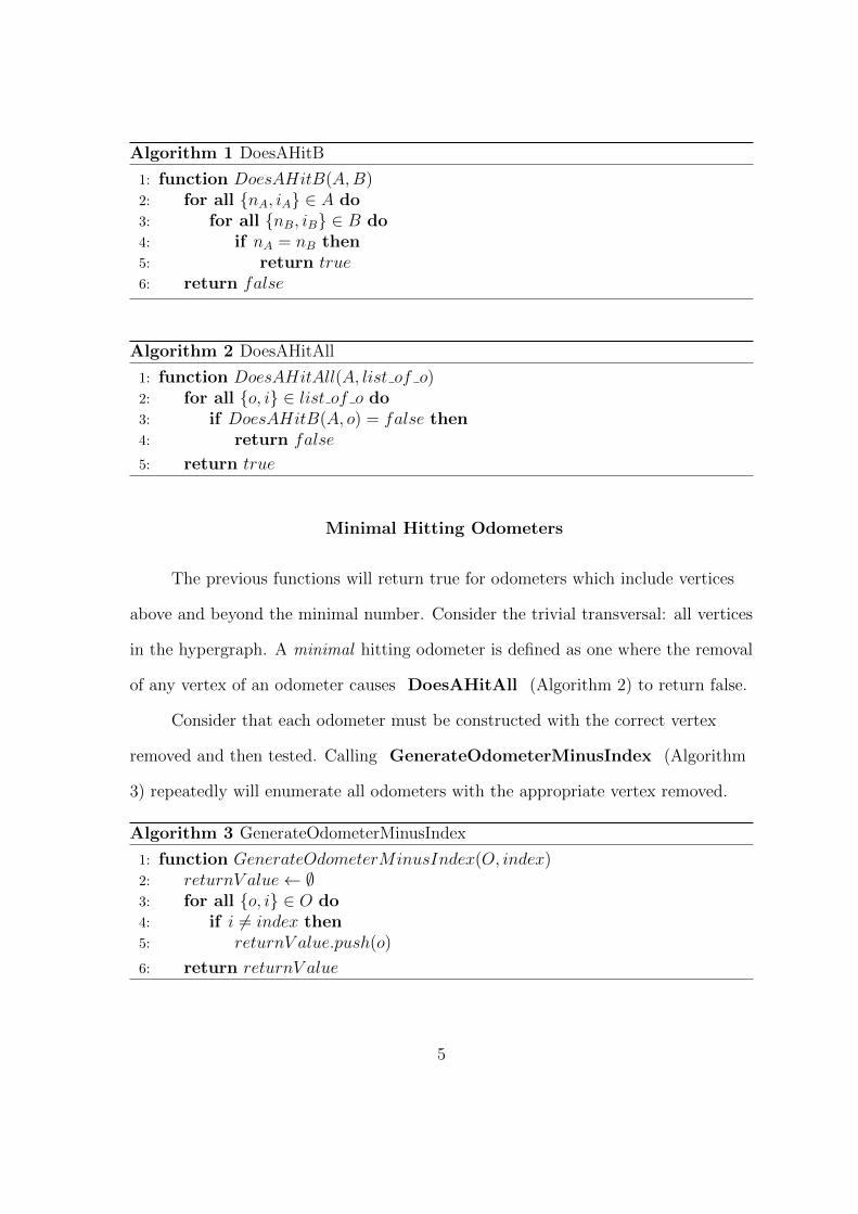
The traditional hitting set calculations are now defined in terms of odometers.

The DoesAHitB (Algorithm 1) answers the question: “does odometer A hit

odometer B”. If A contains a number that is equal to a number in B, then A hits

B. The DoesAHitAll (Algorithm 2) answers the question “does odometer A hit

all of the odometers in a list” by leveraging DoesAHitB (Algorithm 1).

4

Algorithm 1 DoesAHitB

1: function DoesAHitB(A,B)2: for all {nA, iA} ∈ A do3: for all {nB, iB} ∈ B do4: if nA = nB then5: return true6: return false

Algorithm 2 DoesAHitAll

1: function DoesAHitAll(A, list of o)2: for all {o, i} ∈ list of o do3: if DoesAHitB(A, o) = false then4: return false

5: return true

Minimal Hitting Odometers

The previous functions will return true for odometers which include vertices

above and beyond the minimal number. Consider the trivial transversal: all vertices

in the hypergraph. A minimal hitting odometer is defined as one where the removal

of any vertex of an odometer causes DoesAHitAll (Algorithm 2) to return false.

Consider that each odometer must be constructed with the correct vertex

removed and then tested. Calling GenerateOdometerMinusIndex (Algorithm

3) repeatedly will enumerate all odometers with the appropriate vertex removed.

Algorithm 3 GenerateOdometerMinusIndex

1: function GenerateOdometerMinusIndex(O, index)2: returnV alue← ∅3: for all {o, i} ∈ O do4: if i 6= index then5: returnV alue.push(o)

6: return returnV alue

5

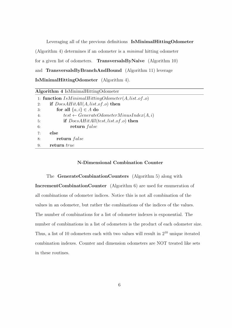
Leveraging all of the previous definitions IsMinimalHittingOdometer

(Algorithm 4) determines if an odometer is a minimal hitting odometer

for a given list of odometers. TransversalsByNaive (Algorithm 10)

and TransversalsByBranchAndBound (Algorithm 11) leverage

IsMinimalHittingOdometer (Algorithm 4).

Algorithm 4 IsMinimalHittingOdometer

1: function IsMinimalHittingOdometer(A, list of o)2: if DoesAHitAll(A, list of o) then3: for all {a, i} ∈ A do4: test← GenerateOdometerMinusIndex(A, i)5: if DoesAHitAll(test, list of o) then6: return false

7: else8: return false

9: return true

N-Dimensional Combination Counter

The GenerateCombinationCounters (Algorithm 5) along with

IncrementCombinationCounter (Algorithm 6) are used for enumeration of

all combinations of odometer indices. Notice this is not all combination of the

values in an odometer, but rather the combinations of the indices of the values.

The number of combinations for a list of odometer indexes is exponential. The

number of combinations in a list of odometers is the product of each odometer size.

Thus, a list of 10 odometers each with two values will result in 210 unique iterated

combination indexes. Counter and dimension odometers are NOT treated like sets

in these routines.

6

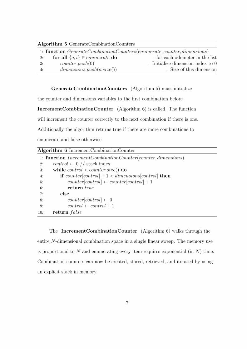
Algorithm 5 GenerateCombinationCounters

1: function GenerateCombinationCounters(enumerate, counter, dimensions)2: for all {o, i} ∈ enumerate do . for each odometer in the list3: counter.push(0) . Initialize dimension index to 04: dimensions.push(o.size()) . Size of this dimension

GenerateCombinationCounters (Algorithm 5) must initialize

the counter and dimensions variables to the first combination before

IncrementCombinationCounter (Algorithm 6) is called. The function

will increment the counter correctly to the next combination if there is one.

Additionally the algorithm returns true if there are more combinations to

enumerate and false otherwise.

Algorithm 6 IncrementCombinationCounter

1: function IncrementCombinationCounter(counter, dimensions)2: control← 0 // stack index3: while control < counter.size() do4: if counter[control] + 1 < dimensions[control] then5: counter[control]← counter[control] + 16: return true7: else8: counter[control]← 09: control← control + 1

10: return false

The IncrementCombinationCounter (Algorithm 6) walks through the

entire N -dimensional combination space in a single linear sweep. The memory use

is proportional to N and enumerating every item requires exponential (in N) time.

Combination counters can now be created, stored, retrieved, and iterated by using

an explicit stack in memory.

7

CHAPTER III

HYPERGRAPHS

Hypergraphs are a recent mathematical discovery which model complex

combination and permutation structures. The number of potential edges in a

normal hypergraph is 2N . Traditionally a hypergraph is defined as a collection H

of sets H = (V,E) where V is a set of vertices and E is a set of hyperedges. There

is no ordering and no repeated hyperedges or vertices. Abstracting from a normal

to an unrestricted hypergraph allows the edges to grow unbounded N∞. There

are only two algorithms presented in this paper that reason about unrestricted

hypergraphs, and then restrictions are put in place for the rest of the algorithms.

Unrestricted Hypergraphs

Definition 3.1.1. Let a hyperedge e be a list of vertices: e = {v, i}. The ith vertex

of e can be written vi = e[i]. Vertices v can be repeated, as they are distinguished

via their index. Indices i are unique non-repeating whole numbers from [0,∞]. The

size of the hyperedge written as e.size() is the count of {v, i}.

Definition 3.1.2. Let an unrestricted hypergraph U be a single hyperedge nodes

and the two functions OtoE and EtoO. OtoE is the surjective function to map

a given odometer to a hyperedge. EtoO is the injective function to map a given

hyperedge to an odometer. The hyperedge U.nodes cannot repeat any vertexes v

for the function EtoO to behave correctly.

Given these definitions, the following is possible given a hypergraph: a

hyperedge can be constructed from an odometer, and an odometer can be

constructed from a hyperedge. Thus, every instance of a hyperedge can be

8

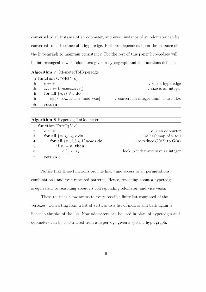
converted to an instance of an odometer, and every instance of an odometer can be

converted to an instance of a hyperedge. Both are dependent upon the instance of

the hypergraph to maintain consistency. For the rest of this paper hyperedges will

be interchangeable with odometers given a hypergraph and the functions defined.

Algorithm 7 OdometerToHyperedge

1: function OtoE(U, o)2: e← ∅ . e is a hyperedge3: size← U.nodes.size() . size is an integer4: for all {n, i} ∈ o do5: e[i]← U.nodes[n mod size] . convert an integer number to index

6: return e

Algorithm 8 HyperedgeToOdometer

1: function EtoO(U, e)2: o← ∅ . o is an odometer3: for all {ve, ie} ∈ e do . use hashmap of v to i4: for all {vn, in} ∈ U.nodes do . to reduce O(n2) to O(n)5: if ve = vn then6: o[ie]← in . lookup index and save as integer

7: return o

Notice that these functions provide liner time access to all permutations,

combinations, and even repeated patterns. Hence, reasoning about a hyperedge

is equivalent to reasoning about its corresponding odometer, and vice versa.

These routines allow access to every possible finite list composed of the

vertexes. Converting from a list of vertices to a list of indices and back again is

linear in the size of the list. Now odometers can be used in place of hyperedges and

odometers can be constructed from a hyperedge given a specific hypergraph.

9

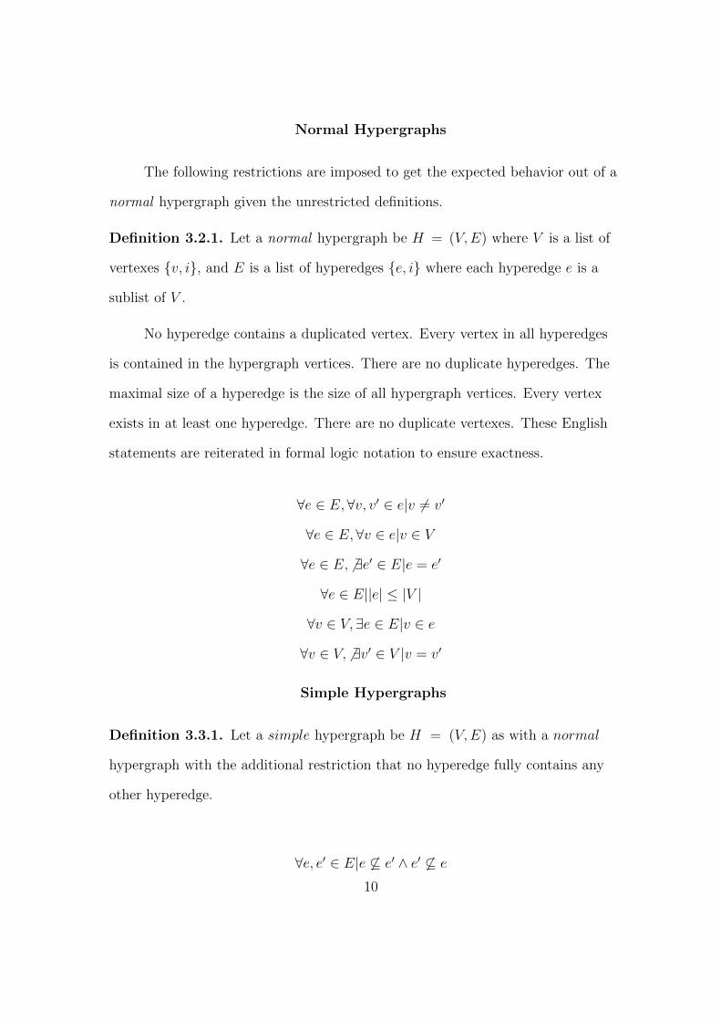
Normal Hypergraphs

The following restrictions are imposed to get the expected behavior out of a

normal hypergraph given the unrestricted definitions.

Definition 3.2.1. Let a normal hypergraph be H = (V,E) where V is a list of

vertexes {v, i}, and E is a list of hyperedges {e, i} where each hyperedge e is a

sublist of V .

No hyperedge contains a duplicated vertex. Every vertex in all hyperedges

is contained in the hypergraph vertices. There are no duplicate hyperedges. The

maximal size of a hyperedge is the size of all hypergraph vertices. Every vertex

exists in at least one hyperedge. There are no duplicate vertexes. These English

statements are reiterated in formal logic notation to ensure exactness.

∀e ∈ E,∀v, v′ ∈ e|v 6= v′

∀e ∈ E,∀v ∈ e|v ∈ V

∀e ∈ E, 6 ∃e′ ∈ E|e = e′

∀e ∈ E||e| ≤ |V |

∀v ∈ V, ∃e ∈ E|v ∈ e

∀v ∈ V, 6 ∃v′ ∈ V |v = v′

Simple Hypergraphs

Definition 3.3.1. Let a simple hypergraph be H = (V,E) as with a normal

hypergraph with the additional restriction that no hyperedge fully contains any

other hyperedge.

∀e, e′ ∈ E|e 6⊆ e′ ∧ e′ 6⊆ e

10

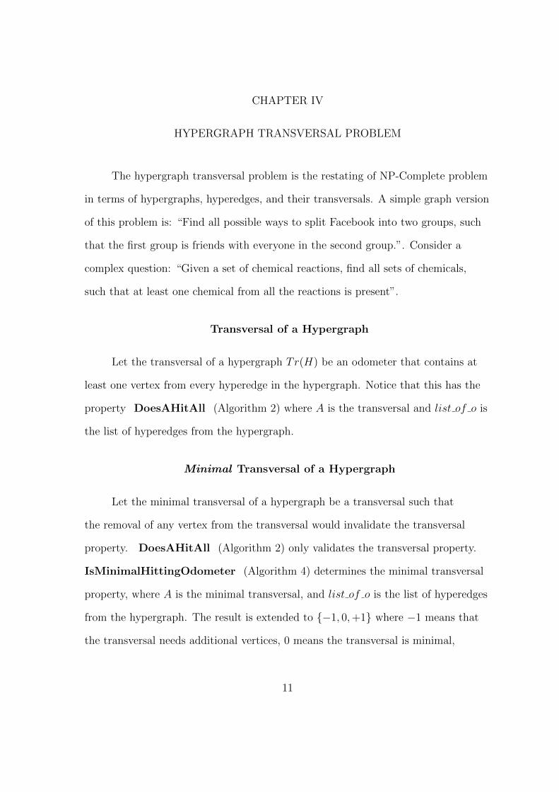
CHAPTER IV

HYPERGRAPH TRANSVERSAL PROBLEM

The hypergraph transversal problem is the restating of NP-Complete problem

in terms of hypergraphs, hyperedges, and their transversals. A simple graph version

of this problem is: “Find all possible ways to split Facebook into two groups, such

that the first group is friends with everyone in the second group.”. Consider a

complex question: “Given a set of chemical reactions, find all sets of chemicals,

such that at least one chemical from all the reactions is present”.

Transversal of a Hypergraph

Let the transversal of a hypergraph Tr(H) be an odometer that contains at

least one vertex from every hyperedge in the hypergraph. Notice that this has the

property DoesAHitAll (Algorithm 2) where A is the transversal and list of o is

the list of hyperedges from the hypergraph.

Minimal Transversal of a Hypergraph

Let the minimal transversal of a hypergraph be a transversal such that

the removal of any vertex from the transversal would invalidate the transversal

property. DoesAHitAll (Algorithm 2) only validates the transversal property.

IsMinimalHittingOdometer (Algorithm 4) determines the minimal transversal

property, where A is the minimal transversal, and list of o is the list of hyperedges

from the hypergraph. The result is extended to {−1, 0,+1} where −1 means that

the transversal needs additional vertices, 0 means the transversal is minimal,

11

and +1 means that there is a minimal transversal that is contained inside of this

transversal.

Algorithm 9 IsMinimalTransversal

1: function IsMinimalTransversal(O, list of o)2: if DoesAHitAll(O, list of o) = false then3: return −1

4: for all {o, i} ∈ O do5: test← GenerateOdometerMinusIndex(O, i)6: if DoesAHitAll(test, list of o) then7: return 18: return 0

12

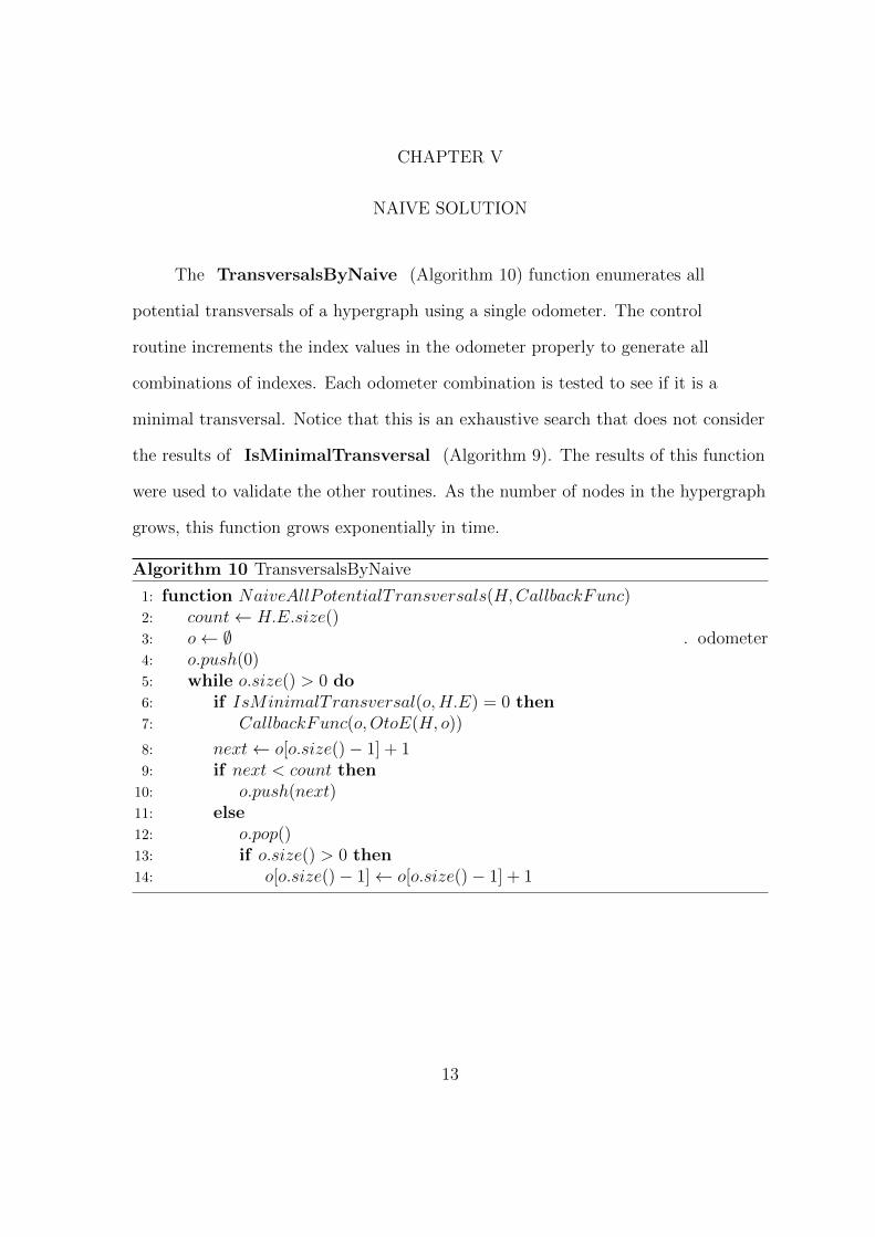
CHAPTER V

NAIVE SOLUTION

The TransversalsByNaive (Algorithm 10) function enumerates all

potential transversals of a hypergraph using a single odometer. The control

routine increments the index values in the odometer properly to generate all

combinations of indexes. Each odometer combination is tested to see if it is a

minimal transversal. Notice that this is an exhaustive search that does not consider

the results of IsMinimalTransversal (Algorithm 9). The results of this function

were used to validate the other routines. As the number of nodes in the hypergraph

grows, this function grows exponentially in time.

Algorithm 10 TransversalsByNaive

1: function NaiveAllPotentialTransversals(H,CallbackFunc)2: count← H.E.size()3: o← ∅ . odometer4: o.push(0)5: while o.size() > 0 do6: if IsMinimalTransversal(o,H.E) = 0 then7: CallbackFunc(o,OtoE(H, o))

8: next← o[o.size()− 1] + 19: if next < count then10: o.push(next)11: else12: o.pop()13: if o.size() > 0 then14: o[o.size()− 1]← o[o.size()− 1] + 1

13

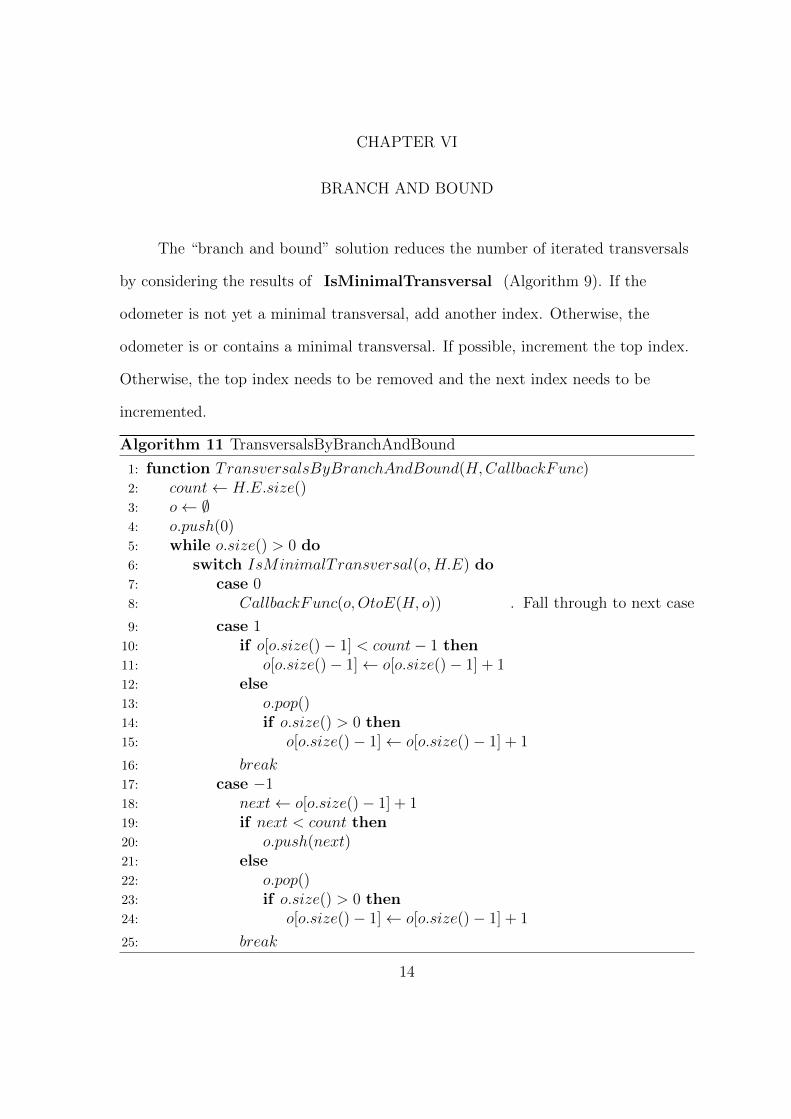
CHAPTER VI

BRANCH AND BOUND

The “branch and bound” solution reduces the number of iterated transversals

by considering the results of IsMinimalTransversal (Algorithm 9). If the

odometer is not yet a minimal transversal, add another index. Otherwise, the

odometer is or contains a minimal transversal. If possible, increment the top index.

Otherwise, the top index needs to be removed and the next index needs to be

incremented.

Algorithm 11 TransversalsByBranchAndBound

1: function TransversalsByBranchAndBound(H,CallbackFunc)2: count← H.E.size()3: o← ∅4: o.push(0)5: while o.size() > 0 do6: switch IsMinimalTransversal(o,H.E) do7: case 08: CallbackFunc(o,OtoE(H, o)) . Fall through to next case

9: case 110: if o[o.size()− 1] < count− 1 then11: o[o.size()− 1]← o[o.size()− 1] + 112: else13: o.pop()14: if o.size() > 0 then15: o[o.size()− 1]← o[o.size()− 1] + 1

16: break17: case −118: next← o[o.size()− 1] + 119: if next < count then20: o.push(next)21: else22: o.pop()23: if o.size() > 0 then24: o[o.size()− 1]← o[o.size()− 1] + 1

25: break

14

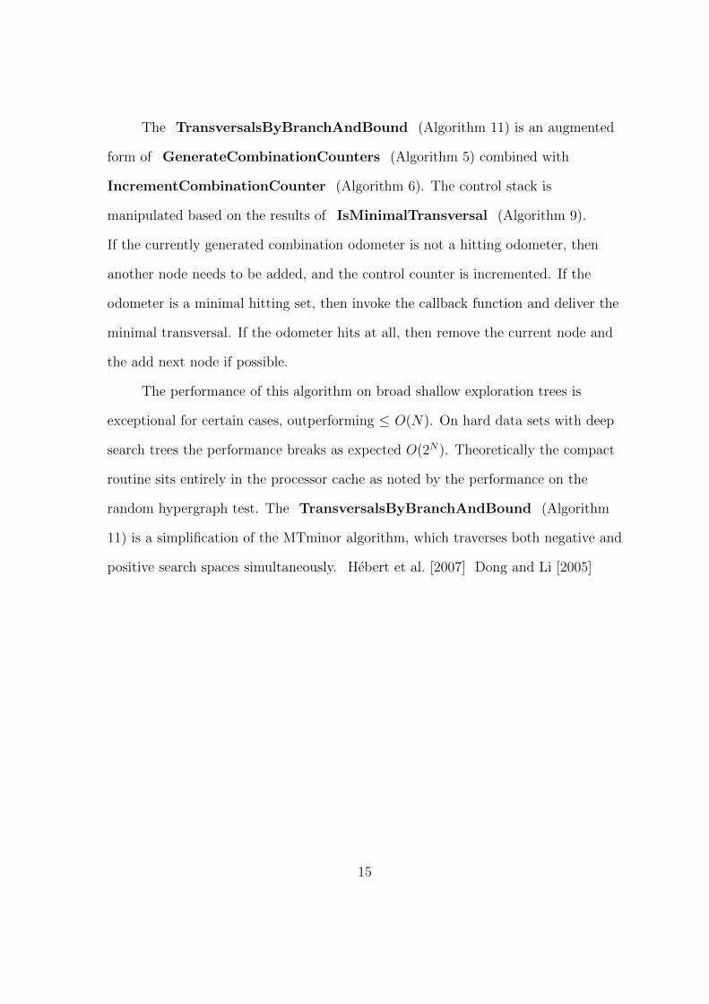
The TransversalsByBranchAndBound (Algorithm 11) is an augmented

form of GenerateCombinationCounters (Algorithm 5) combined with

IncrementCombinationCounter (Algorithm 6). The control stack is

manipulated based on the results of IsMinimalTransversal (Algorithm 9).

If the currently generated combination odometer is not a hitting odometer, then

another node needs to be added, and the control counter is incremented. If the

odometer is a minimal hitting set, then invoke the callback function and deliver the

minimal transversal. If the odometer hits at all, then remove the current node and

the add next node if possible.

The performance of this algorithm on broad shallow exploration trees is

exceptional for certain cases, outperforming ≤ O(N). On hard data sets with deep

search trees the performance breaks as expected O(2N). Theoretically the compact

routine sits entirely in the processor cache as noted by the performance on the

random hypergraph test. The TransversalsByBranchAndBound (Algorithm

11) is a simplification of the MTminor algorithm, which traverses both negative and

positive search spaces simultaneously. Hebert et al. [2007] Dong and Li [2005]

15

CHAPTER VII

DYNAMIC SOLUTION

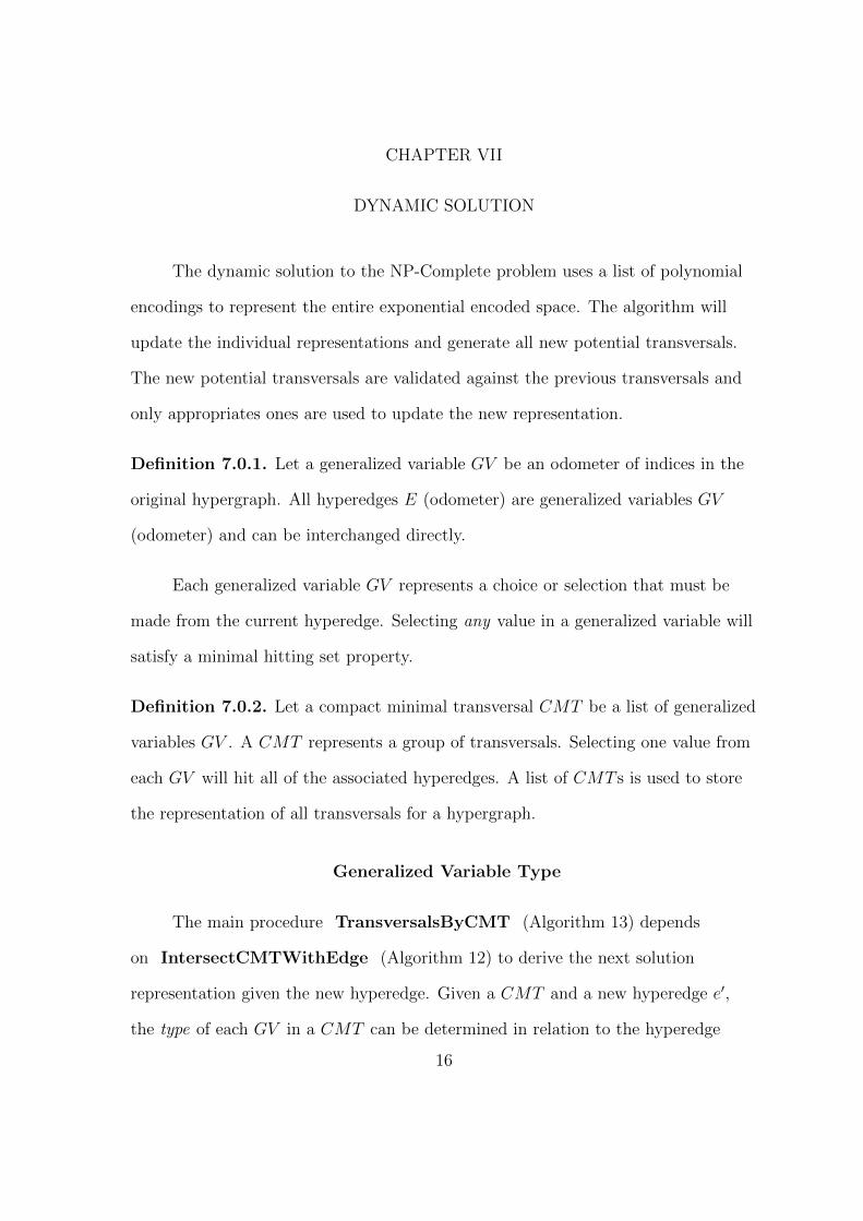
The dynamic solution to the NP-Complete problem uses a list of polynomial

encodings to represent the entire exponential encoded space. The algorithm will

update the individual representations and generate all new potential transversals.

The new potential transversals are validated against the previous transversals and

only appropriates ones are used to update the new representation.

Definition 7.0.1. Let a generalized variable GV be an odometer of indices in the

original hypergraph. All hyperedges E (odometer) are generalized variables GV

(odometer) and can be interchanged directly.

Each generalized variable GV represents a choice or selection that must be

made from the current hyperedge. Selecting any value in a generalized variable will

satisfy a minimal hitting set property.

Definition 7.0.2. Let a compact minimal transversal CMT be a list of generalized

variables GV . A CMT represents a group of transversals. Selecting one value from

each GV will hit all of the associated hyperedges. A list of CMT s is used to store

the representation of all transversals for a hypergraph.

Generalized Variable Type

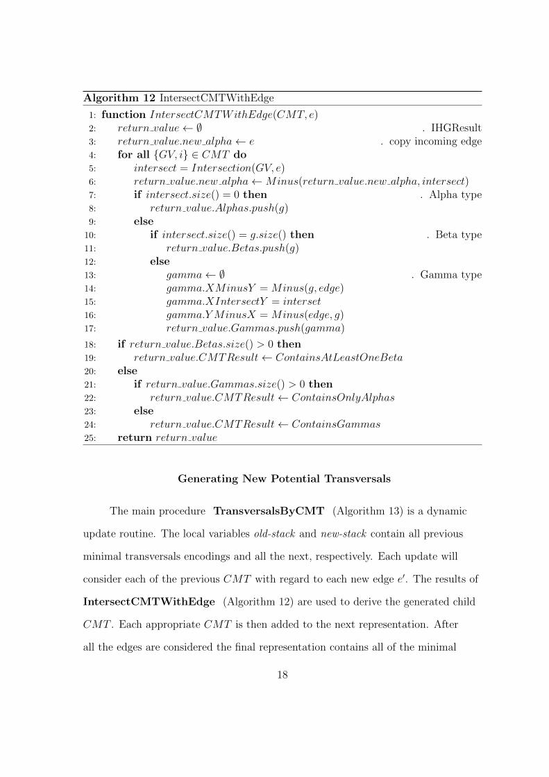
The main procedure TransversalsByCMT (Algorithm 13) depends

on IntersectCMTWithEdge (Algorithm 12) to derive the next solution

representation given the new hyperedge. Given a CMT and a new hyperedge e′,

the type of each GV in a CMT can be determined in relation to the hyperedge

16

e′. The type is used to generate all of the child minimal transversals in the main

procedure.

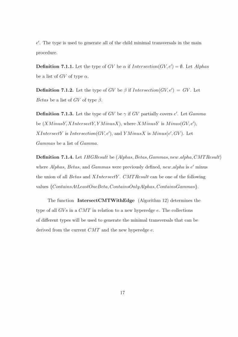
Definition 7.1.1. Let the type of GV be α if Intersection(GV, e′) = ∅. Let Alphas

be a list of GV of type α.

Definition 7.1.2. Let the type of GV be β if Intersection(GV, e′) = GV . Let

Betas be a list of GV of type β.

Definition 7.1.3. Let the type of GV be γ if GV partially covers e′. Let Gamma

be (XMinusY,XIntersectY, Y MinusX), where XMinusY is Minus(GV, e′),

XIntersectY is Intersection(GV, e′), and YMinusX is Minus(e′, GV ). Let

Gammas be a list of Gamma.

Definition 7.1.4. Let IHGResult be (Alphas,Betas,Gammas, new alpha, CMTResult)

where Alphas, Betas, and Gammas were previously defined, new alpha is e′ minus

the union of all Betas and XIntersectY . CMTResult can be one of the following

values {ContainsAtLeastOneBeta, ContainsOnlyAlphas, ContainsGammas}.

The function IntersectCMTWithEdge (Algorithm 12) determines the

type of all GV s in a CMT in relation to a new hyperedge e. The collections

of different types will be used to generate the minimal transversals that can be

derived from the current CMT and the new hyperedge e.

17

Algorithm 12 IntersectCMTWithEdge

1: function IntersectCMTWithEdge(CMT, e)2: return value← ∅ . IHGResult3: return value.new alpha← e . copy incoming edge4: for all {GV, i} ∈ CMT do5: intersect = Intersection(GV, e)6: return value.new alpha←Minus(return value.new alpha, intersect)7: if intersect.size() = 0 then . Alpha type8: return value.Alphas.push(g)9: else10: if intersect.size() = g.size() then . Beta type11: return value.Betas.push(g)12: else13: gamma← ∅ . Gamma type14: gamma.XMinusY = Minus(g, edge)15: gamma.XIntersectY = interset16: gamma.YMinusX = Minus(edge, g)17: return value.Gammas.push(gamma)

18: if return value.Betas.size() > 0 then19: return value.CMTResult← ContainsAtLeastOneBeta20: else21: if return value.Gammas.size() > 0 then22: return value.CMTResult← ContainsOnlyAlphas23: else24: return value.CMTResult← ContainsGammas25: return return value

Generating New Potential Transversals

The main procedure TransversalsByCMT (Algorithm 13) is a dynamic

update routine. The local variables old-stack and new-stack contain all previous

minimal transversals encodings and all the next, respectively. Each update will

consider each of the previous CMT with regard to each new edge e′. The results of

IntersectCMTWithEdge (Algorithm 12) are used to derive the generated child

CMT . Each appropriate CMT is then added to the next representation. After

all the edges are considered the final representation contains all of the minimal

18

transversals of the hypergraph. Lastly, calling ExtractTransversals (Algorithm

18) for each CMT enumerates all of the transversals in the representation. The

original proof with complete mathematical details is available in the previous works

Kavvadias and Stavropoulos [2005]. Unfortunately, restructuring these proofs for

this paper is beyond ability of the author at this time.

If there are any GV of type Beta then the current CMT will always hit the

new edge. All the transversals in the CMT will hit the new edge. Hence, we add

the CMT to the next list of transversals.

If there are no Gamma, then all GV are of type Alpha. Each piecewise item

in the new edge e′ needs to be added to each of the transversals in the CMT

and considered as a child CMT . Each new child CMT contains a single GV

containing a single node from the edge. The newly generated child transversal

now hits the new edge but it may contain a non-minimal transversal that needs

to be removed. ProcessNewCMT (Algorithm 17) handles the removal of

inappropriate transversals and the updates to the representation.

If there are any Gamma, then there are 2|Gamma| possible combinations of

intersecting and non-intersecting GV that need to be considered. There is the

special outer section case that needs to be considered first when there are both

intersecting parts and also new nodes to pick from. When picking all of the outer

sections of the Gamma, for each new Alpha, we add a new child CMT . Next,

initialize the counters and iterate all of the exponential combinations that hit

the new edge e′. For each of the newly generated combinations, they can contain

transversals that are non-minimal transversals. ProcessNewCMT (Algorithm

17) handles the removal of inappropriate transversals and updates the next

representation.

19

ExtractTransversals (Algorithm 18) is leveraged to enumerate the

entire CMT representation, passing each transversal to the visitor function. The

mundane helper functions GenNextAlpha (Algorithm 14), GenFirstGamma

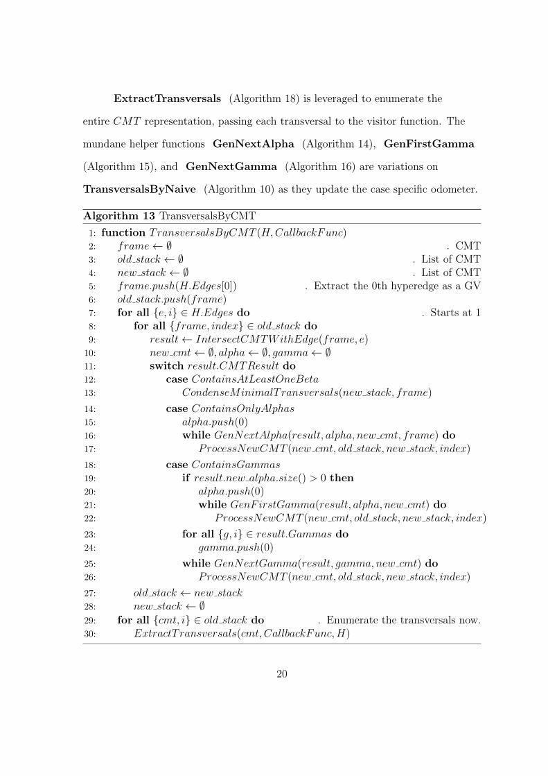
(Algorithm 15), and GenNextGamma (Algorithm 16) are variations on

TransversalsByNaive (Algorithm 10) as they update the case specific odometer.

Algorithm 13 TransversalsByCMT

1: function TransversalsByCMT (H,CallbackFunc)2: frame← ∅ . CMT3: old stack ← ∅ . List of CMT4: new stack ← ∅ . List of CMT5: frame.push(H.Edges[0]) . Extract the 0th hyperedge as a GV6: old stack.push(frame)7: for all {e, i} ∈ H.Edges do . Starts at 18: for all {frame, index} ∈ old stack do9: result← IntersectCMTWithEdge(frame, e)10: new cmt← ∅, alpha← ∅, gamma← ∅11: switch result.CMTResult do12: case ContainsAtLeastOneBeta13: CondenseMinimalTransversals(new stack, frame)

14: case ContainsOnlyAlphas15: alpha.push(0)16: while GenNextAlpha(result, alpha, new cmt, frame) do17: ProcessNewCMT (new cmt, old stack, new stack, index)

18: case ContainsGammas19: if result.new alpha.size() > 0 then20: alpha.push(0)21: while GenFirstGamma(result, alpha, new cmt) do22: ProcessNewCMT (new cmt, old stack, new stack, index)

23: for all {g, i} ∈ result.Gammas do24: gamma.push(0)

25: while GenNextGamma(result, gamma, new cmt) do26: ProcessNewCMT (new cmt, old stack, new stack, index)

27: old stack ← new stack28: new stack ← ∅29: for all {cmt, i} ∈ old stack do . Enumerate the transversals now.30: ExtractTransversals(cmt, CallbackFunc,H)

20

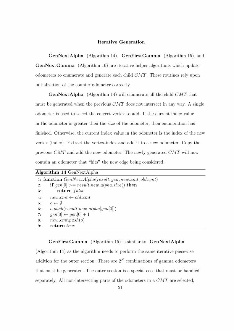
Iterative Generation

GenNextAlpha (Algorithm 14), GenFirstGamma (Algorithm 15), and

GenNextGamma (Algorithm 16) are iterative helper algorithms which update

odometers to enumerate and generate each child CMT . These routines rely upon

initialization of the counter odometer correctly.

GenNextAlpha (Algorithm 14) will enumerate all the child CMT that

must be generated when the previous CMT does not intersect in any way. A single

odometer is used to select the correct vertex to add. If the current index value

in the odometer is greater then the size of the odometer, then enumeration has

finished. Otherwise, the current index value in the odometer is the index of the new

vertex (index). Extract the vertex-index and add it to a new odometer. Copy the

previous CMT and add the new odometer. The newly generated CMT will now

contain an odometer that “hits” the new edge being considered.

Algorithm 14 GenNextAlpha

1: function GenNextAlpha(result, gen, new cmt, old cmt)2: if gen[0] >= result.new alpha.size() then3: return false

4: new cmt← old cmt5: o← ∅6: o.push(result.new alpha[gen[0]])7: gen[0]← gen[0] + 18: new cmt.push(o)9: return true

GenFirstGamma (Algorithm 15) is similar to GenNextAlpha

(Algorithm 14) as the algorithm needs to perform the same iterative piecewise

addition for the outer section. There are 2N combinations of gamma odometers

that must be generated. The outer section is a special case that must be handled

separately. All non-intersecting parts of the odometers in a CMT are selected,

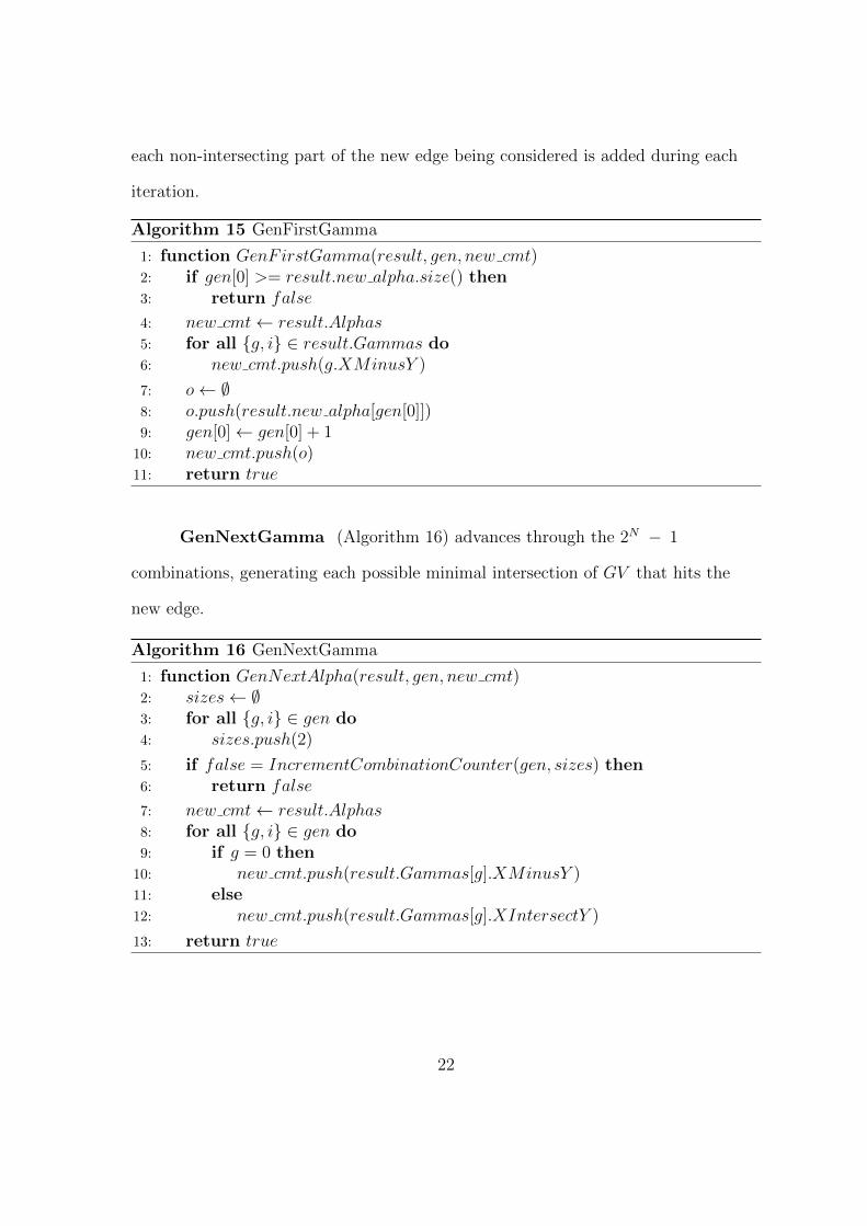
21

each non-intersecting part of the new edge being considered is added during each

iteration.

Algorithm 15 GenFirstGamma

1: function GenFirstGamma(result, gen, new cmt)2: if gen[0] >= result.new alpha.size() then3: return false

4: new cmt← result.Alphas5: for all {g, i} ∈ result.Gammas do6: new cmt.push(g.XMinusY )

7: o← ∅8: o.push(result.new alpha[gen[0]])9: gen[0]← gen[0] + 110: new cmt.push(o)11: return true

GenNextGamma (Algorithm 16) advances through the 2N − 1

combinations, generating each possible minimal intersection of GV that hits the

new edge.

Algorithm 16 GenNextGamma

1: function GenNextAlpha(result, gen, new cmt)2: sizes← ∅3: for all {g, i} ∈ gen do4: sizes.push(2)

5: if false = IncrementCombinationCounter(gen, sizes) then6: return false

7: new cmt← result.Alphas8: for all {g, i} ∈ gen do9: if g = 0 then10: new cmt.push(result.Gammas[g].XMinusY )11: else12: new cmt.push(result.Gammas[g].XIntersectY )

13: return true

22

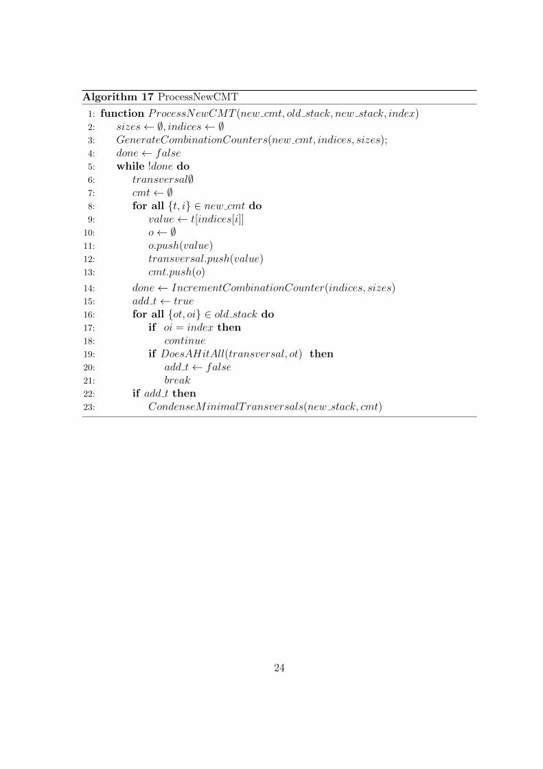
Processing New Transversals

All new potential minimal transversals are now properly generated by the

preceding routines. Each of the new potential minimal transversals needs to be

considered in order to see if the child should actually be added to the next set

of real minimal transversals. If any new potential minimal transversal hits any

previous minimal transversal then the newly generated child is not appropriate,

as noted in previous work by Kavvadias and Stavropoulos [1999, 2005].

All transversals in a child CMT must be extracted and considered in

order to determine if it hits a previous transversal. An interesting result is that

not all previous transversals need be extracted from each CMT . A transversal

that hits every GV in a CMT is not an appropriate transversal to be added.

ProcessNewCMT (Algorithm 17) extracts all transversals from the CMT and

if any hit a previous CMT they not added to the next solution list of CMT .

23

Algorithm 17 ProcessNewCMT

1: function ProcessNewCMT (new cmt, old stack, new stack, index)2: sizes← ∅, indices← ∅3: GenerateCombinationCounters(new cmt, indices, sizes);4: done← false5: while !done do6: transversal∅7: cmt← ∅8: for all {t, i} ∈ new cmt do9: value← t[indices[i]]10: o← ∅11: o.push(value)12: transversal.push(value)13: cmt.push(o)

14: done← IncrementCombinationCounter(indices, sizes)15: add t← true16: for all {ot, oi} ∈ old stack do17: if oi = index then18: continue19: if DoesAHitAll(transversal, ot) then20: add t← false21: break22: if add t then23: CondenseMinimalTransversals(new stack, cmt)

24

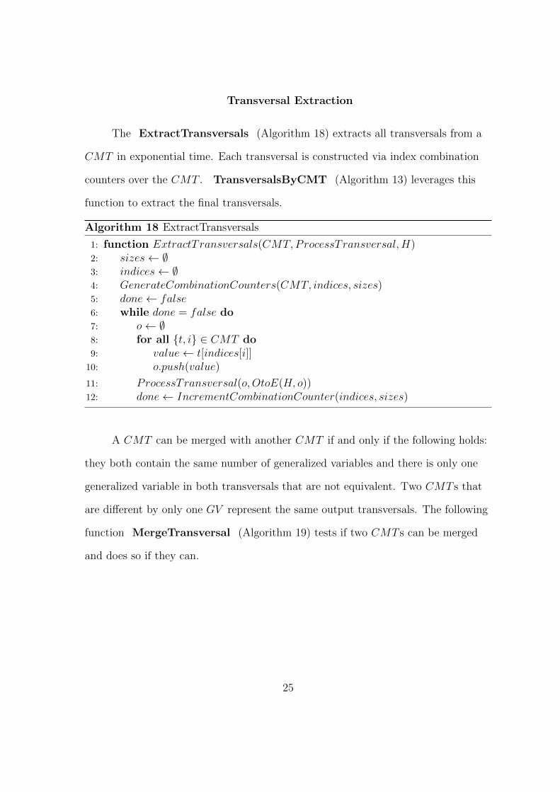
Transversal Extraction

The ExtractTransversals (Algorithm 18) extracts all transversals from a

CMT in exponential time. Each transversal is constructed via index combination

counters over the CMT . TransversalsByCMT (Algorithm 13) leverages this

function to extract the final transversals.

Algorithm 18 ExtractTransversals

1: function ExtractTransversals(CMT,ProcessTransversal,H)2: sizes← ∅3: indices← ∅4: GenerateCombinationCounters(CMT, indices, sizes)5: done← false6: while done = false do7: o← ∅8: for all {t, i} ∈ CMT do9: value← t[indices[i]]10: o.push(value)

11: ProcessTransversal(o,OtoE(H, o))12: done← IncrementCombinationCounter(indices, sizes)

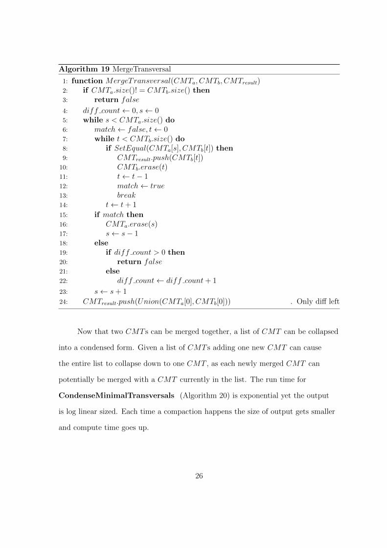
A CMT can be merged with another CMT if and only if the following holds:

they both contain the same number of generalized variables and there is only one

generalized variable in both transversals that are not equivalent. Two CMT s that

are different by only one GV represent the same output transversals. The following

function MergeTransversal (Algorithm 19) tests if two CMT s can be merged

and does so if they can.

25

Algorithm 19 MergeTransversal

1: function MergeTransversal(CMTa, CMTb, CMTresult)2: if CMTa.size()! = CMTb.size() then3: return false

4: diff count← 0, s← 05: while s < CMTa.size() do6: match← false, t← 07: while t < CMTb.size() do8: if SetEqual(CMTa[s], CMTb[t]) then9: CMTresult.push(CMTb[t])10: CMTb.erase(t)11: t← t− 112: match← true13: break14: t← t+ 1

15: if match then16: CMTa.erase(s)17: s← s− 118: else19: if diff count > 0 then20: return false21: else22: diff count← diff count+ 1

23: s← s+ 1

24: CMTresult.push(Union(CMTa[0], CMTb[0])) . Only diff left

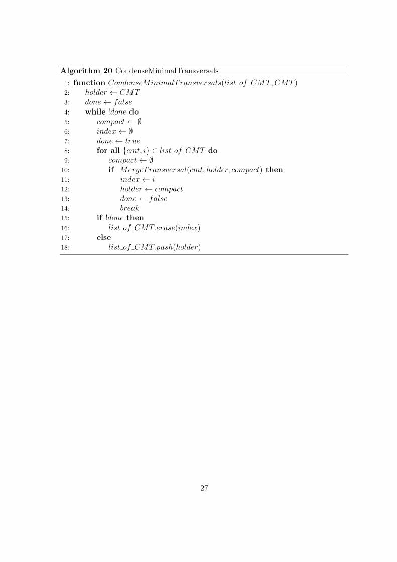
Now that two CMT s can be merged together, a list of CMT can be collapsed

into a condensed form. Given a list of CMT s adding one new CMT can cause

the entire list to collapse down to one CMT , as each newly merged CMT can

potentially be merged with a CMT currently in the list. The run time for

CondenseMinimalTransversals (Algorithm 20) is exponential yet the output

is log linear sized. Each time a compaction happens the size of output gets smaller

and compute time goes up.

26

Algorithm 20 CondenseMinimalTransversals

1: function CondenseMinimalTransversals(list of CMT,CMT )2: holder ← CMT3: done← false4: while !done do5: compact← ∅6: index← ∅7: done← true8: for all {cmt, i} ∈ list of CMT do9: compact← ∅10: if MergeTransversal(cmt, holder, compact) then11: index← i12: holder ← compact13: done← false14: break15: if !done then16: list of CMT.erase(index)17: else18: list of CMT.push(holder)

27

Solution

This concludes the current form of the algorithm designated Norris-Casita-

Dynamic (NC-D). The iterative solution to enumerating all minimal hypergraph

traversals is now complete. Each child CMT has an exponential number of

transversals that are extracted in ProcessNewCMT (Algorithm 17) and added

to the next set of CMT s. There is a shortcut in ProcessNewCMT (Algorithm

17) via the call to DoesAHitAll (Algorithm 2) which eliminates the need to

extract all transversals of the old CMT s.

As each transversal is constructed as a CMT and then added to the list of

CMT s to be collapsed, the enumeration of all minimal transversals at each stage

is guaranteed. The representation of all transversals as a list of CMT is both the

boon and curse of this algorithm. Calls to CondenseMinimalTransversals

(Algorithm 20) are exceedingly expensive because the adjustment to the entire

encoding with regard to the new transversal can take exponential time.

The algorithm differs from the KS algorithm in that all solutions are

computed before the first solution is enumerated. Additionally, the storage of

all transversals as a list of CMT is a dynamic encoding of the solution which is

updated at each iteration.

The KS algorithm uses a similar recursive solution where the call stack grows

polynomial in the edge count. Thus, the algorithm should outperform KS when the

edge count is high enough to offset the penalty for operating on the list of CMT

with CondenseMinimalTransversals (Algorithm 20). The Dual-Matching test

dataset demonstrates this exact result in the results section.

28

CHAPTER VIII

OPTIMIZATION

Chapter VII implements the core algorithms to iteratively generate successive

solution representations. Each representation is updated as it encounters each new

hyperedge. There are different trade offs and potential optimizations with respect

to time and space that will be discussed. However, the authors assume that there

are a class of problems where the additional changes will not be possible. The

additional optimizations exploit the representation that has been built and paid

for with time in CondenseMinimalTransversals (Algorithm 20). One example

is the usage of DoesAHitAll (Algorithm 2) in ProcessNewCMT (Algorithm

17) to eliminate an exponential sub-step by leveraging the representation. Further

polynomial constant exchanges are made for performance enhancements in NC-

DO0, NC-DO1, NC-DO3. The only true optimization is NC-DO3: if the program is

able to output the representation of the solution, instead of the solution.

NC-DO0

ProcessNewCMT (Algorithm 17) enumerates each of the transversals

trying to eliminate the new potential transversal using the previous list of CMT .

Calling CondenseMinimalTransversals (Algorithm 20) on the complete

list of CMT for all child transversals is expensive in time. Removal of any

transversal in a CMT will require a list of CMT to represent the newly reduced

transversals. ProcessNewCMT0 (Algorithm 23) maintains a local list of

CMT that are dynamically updated as they encounter each of the previous

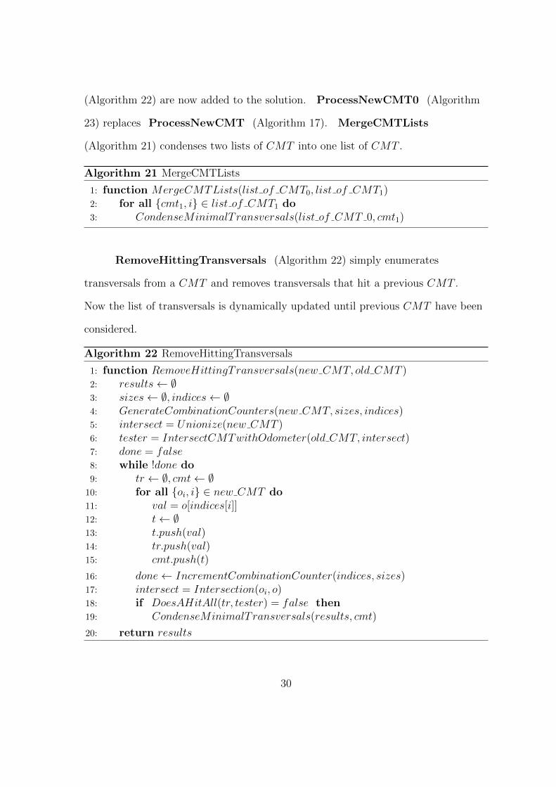
CMT . MergeCMTLists (Algorithm 21) and RemoveHittingTransversals

29

(Algorithm 22) are now added to the solution. ProcessNewCMT0 (Algorithm

23) replaces ProcessNewCMT (Algorithm 17). MergeCMTLists

(Algorithm 21) condenses two lists of CMT into one list of CMT .

Algorithm 21 MergeCMTLists

1: function MergeCMTLists(list of CMT0, list of CMT1)2: for all {cmt1, i} ∈ list of CMT1 do3: CondenseMinimalTransversals(list of CMT 0, cmt1)

RemoveHittingTransversals (Algorithm 22) simply enumerates

transversals from a CMT and removes transversals that hit a previous CMT .

Now the list of transversals is dynamically updated until previous CMT have been

considered.

Algorithm 22 RemoveHittingTransversals

1: function RemoveHittingTransversals(new CMT, old CMT )2: results← ∅3: sizes← ∅, indices← ∅4: GenerateCombinationCounters(new CMT, sizes, indices)5: intersect = Unionize(new CMT )6: tester = IntersectCMTwithOdometer(old CMT, intersect)7: done = false8: while !done do9: tr ← ∅, cmt← ∅10: for all {oi, i} ∈ new CMT do11: val = o[indices[i]]12: t← ∅13: t.push(val)14: tr.push(val)15: cmt.push(t)

16: done← IncrementCombinationCounter(indices, sizes)17: intersect = Intersection(oi, o)18: if DoesAHitAll(tr, tester) = false then19: CondenseMinimalTransversals(results, cmt)

20: return results

30

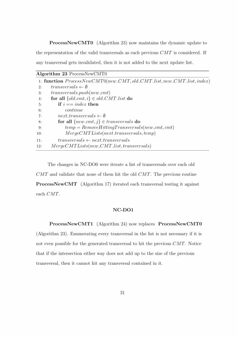
ProcessNewCMT0 (Algorithm 23) now maintains the dynamic update to

the representation of the valid transversals as each previous CMT is considered. If

any transversal gets invalidated, then it is not added to the next update list.

Algorithm 23 ProcessNewCMT0

1: function ProcessNewCMT0(new CMT, old CMT list, new CMT list, index)2: transversals← ∅3: transversals.push(new cmt)4: for all {old cmt, i} ∈ old CMT list do5: if i == index then6: continue7: next transversals← ∅8: for all {new cmt, j} ∈ transversals do9: temp = RemoveHittingTransversals(new cmt, cmt)10: MergeCMTLists(next transversals, temp)

11: transversals← next transversals12: MergeCMTLists(new CMT list, transversals)

The changes in NC-DO0 were iterate a list of transversals over each old

CMT and validate that none of them hit the old CMT . The previous routine

ProcessNewCMT (Algorithm 17) iterated each transversal testing it against

each CMT .

NC-DO1

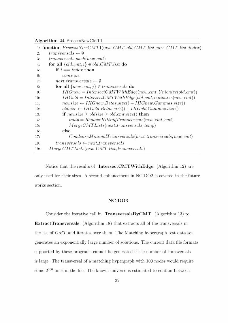
ProcessNewCMT1 (Algorithm 24) now replaces ProcessNewCMT0

(Algorithm 23). Enumerating every transversal in the list is not necessary if it is

not even possible for the generated transversal to hit the previous CMT . Notice

that if the intersection either way does not add up to the size of the previous

transversal, then it cannot hit any transversal contained in it.

31

Algorithm 24 ProcessNewCMT1

1: function ProcessNewCMT1(new CMT, old CMT list, new CMT list, index)2: transversals← ∅3: transversals.push(new cmt)4: for all {old cmt, i} ∈ old CMT list do5: if i == index then6: continue7: next transversals← ∅8: for all {new cmt, j} ∈ transversals do9: IHGnew = IntersectCMTWithEdge(new cmt, Unionize(old cmt))10: IHGold = IntersectCMTWithEdge(old cmt, Unionize(new cmt))11: newsize← IHGnew.Betas.size() + IHGnew.Gammas.size()12: oldsize← IHGold.Betas.size() + IHGold.Gammas.size()13: if newsize ≥ oldsize ≥ old cmt.size() then14: temp = RemoveHittingTransversals(new cmt, cmt)15: MergeCMTLists(next transversals, temp)16: else17: CondenseMinimalTransversals(next transversals, new cmt)

18: transversals← next transversals19: MergeCMTLists(new CMT list, transversals)

Notice that the results of IntersectCMTWithEdge (Algorithm 12) are

only used for their sizes. A second enhancement in NC-DO2 is covered in the future

works section.

NC-DO3

Consider the iterative call in TransversalsByCMT (Algorithm 13) to

ExtractTransversals (Algorithm 18) that extracts all of the transversals in

the list of CMT and iterates over them. The Matching hypergraph test data set

generates an exponentially large number of solutions. The current data file formats

supported by these programs cannot be generated if the number of transversals

is large. The transversal of a matching hypergraph with 100 nodes would require

some 2100 lines in the file. The known universe is estimated to contain between

32

280 and 2100 atoms. It is a safe assumption that the current file format will be

incapable of representing such a solution. On the other hand, the list of CMT

containing the 2100 solutions can be directly written to disk without enumerating

the solution.

If and only if the encoded representation of the solution is acceptable,

then the results of NC-DO3 are applicable. The only optimization in NC-DO3

over NC-D01 is writing the list of CMT directly to file instead of writing the

interpretation of them to file. This change requires a different call-back function

in TransversalsByCMT (Algorithm 13) that accepts CMT directly.

33

CHAPTER IX

VALIDATION & RESULTS

The system used to test these algorithms was an Intel i7-7700k running at 4.5

Ghz, 64GB of DD4 RAM, and a 400GB Intel NVMe SSD hard drive with 2.5GB/s

throughput. All algorithms where implemented in generic standard template library

C++11. As the nature of this problem relies upon complete enumeration of all

transversals regardless of memory usage, compute time alone is used as the metric

of performance. Inefficient memory usage is reflected in longer execution time

should the virtual memory system be used.

The following validation procedure was used. The naive algorithm results

were collected as control, branch and bound was validated against the naive

control, and last the NC-Dynamic solution was validated against naive as well.

The validation of a single hypergraph in this system consisted of iterating

over the intermediate hypergraphs and testing each one. An intermediate

hypergraph is constructed by taking the original hypergraph and iterating over one

edge, two edges, etc, and constructing a hypergraph from each list of edges. This is

an exponential slowdown in validation but also allows the isolation and repetition

of core flaws during the development process. Specifically a “problem” instance

could be identified by hypergraph number and intermediate number.

The iterative techniques to generate all hypergraphs where connected to the

validation and testing system to prove correctness.The generative functions for

hypergraphs are exponentially-exponential on the order of NN−1N−2...

. Hypergraphs

of size 1,2,3,4,5 and 6 were validated. There were over 6 ∗ 109 hypergraphs of

size 6 and took approximately three days on the test machine running as a single

34

threaded process. Hypergraphs of size 7 - 12 were started and allowed to run which

did not terminate before publication and no errors were detected.

Results

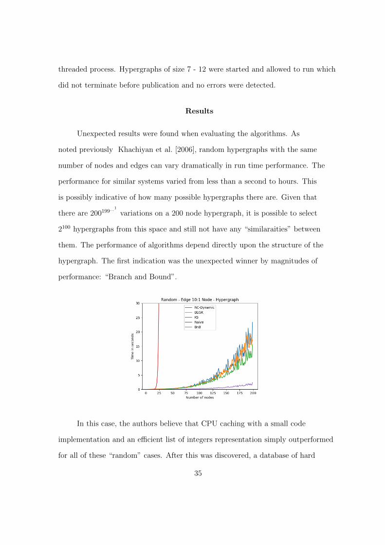
Unexpected results were found when evaluating the algorithms. As

noted previously Khachiyan et al. [2006], random hypergraphs with the same

number of nodes and edges can vary dramatically in run time performance. The

performance for similar systems varied from less than a second to hours. This

is possibly indicative of how many possible hypergraphs there are. Given that

there are 200199...1

variations on a 200 node hypergraph, it is possible to select

2100 hypergraphs from this space and still not have any “similaraities” between

them. The performance of algorithms depend directly upon the structure of the

hypergraph. The first indication was the unexpected winner by magnitudes of

performance: “Branch and Bound”.

In this case, the authors believe that CPU caching with a small code

implementation and an efficient list of integers representation simply outperformed

for all of these “random” cases. After this was discovered, a database of hard

35

hypergraph problems provided by Takeaki Uno was used for the remaining tests

http://research.nii.ac.jp/~uno/dualization.html. The following categories

where examined:

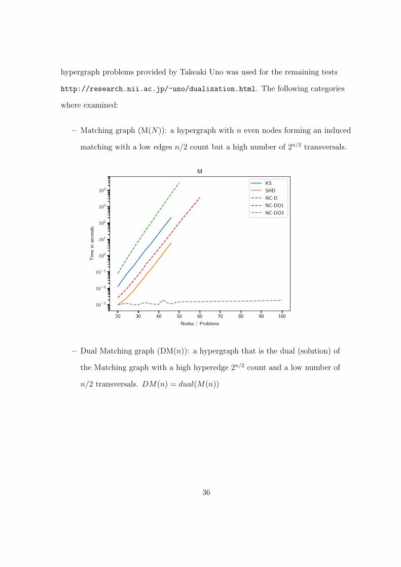
– Matching graph (M(N)): a hypergraph with n even nodes forming an induced

matching with a low edges n/2 count but a high number of 2n/2 transversals.

20 30 40 50 60 70 80 90 100

Nodes / Problems

10−3

10−2

10−1

100

101

102

103

104

Tim

ein

seconds

M

KS

SHD

NC-D

NC-DO1

NC-DO3

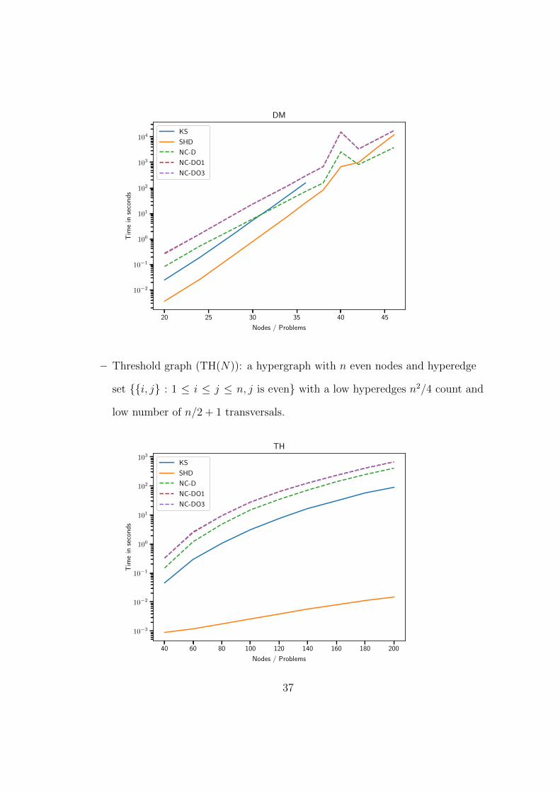
– Dual Matching graph (DM(n)): a hypergraph that is the dual (solution) of

the Matching graph with a high hyperedge 2n/2 count and a low number of

n/2 transversals. DM(n) = dual(M(n))

36

20 25 30 35 40 45

Nodes / Problems

10−2

10−1

100

101

102

103

104Tim

ein

seconds

DM

KS

SHD

NC-D

NC-DO1

NC-DO3

– Threshold graph (TH(N)): a hypergraph with n even nodes and hyperedge

set {{i, j} : 1 ≤ i ≤ j ≤ n, j is even} with a low hyperedges n2/4 count and

low number of n/2 + 1 transversals.

40 60 80 100 120 140 160 180 200

Nodes / Problems

10−3

10−2

10−1

100

101

102

103

Tim

ein

seconds

TH

KS

SHD

NC-D

NC-DO1

NC-DO3

37

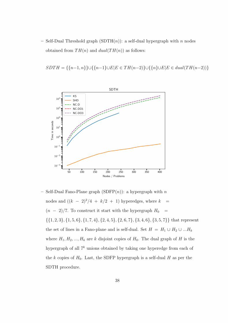
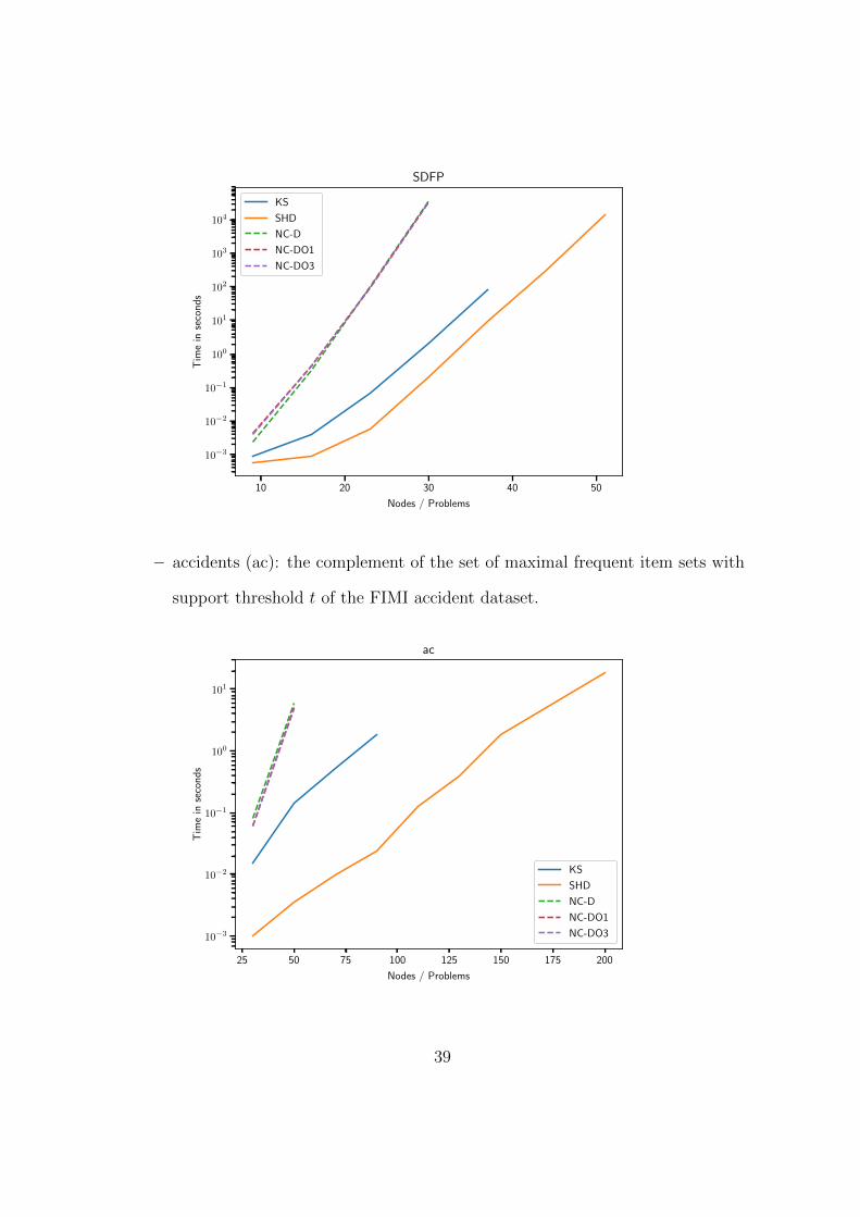
– Self-Dual Threshold graph (SDTH(n)): a self-dual hypergraph with n nodes

obtained from TH(n) and dual(TH(n)) as follows:

SDTH = {{n−1, n}}∪{{n−1}∪E|E ∈ TH(n−2)}∪{{n}∪E|E ∈ dual(TH(n−2))}

50 100 150 200 250 300 350 400

Nodes / Problems

10−3

10−2

10−1

100

101

102

103

104

Tim

ein

seconds

SDTH

KS

SHD

NC-D

NC-DO1

NC-DO3

– Self-Dual Fano-Plane graph (SDFP(n)): a hypergraph with n

nodes and ((k − 2)2/4 + k/2 + 1) hyperedges, where k =

(n − 2)/7. To construct it start with the hypergraph H0 =

{{1, 2, 3}, {1, 5, 6}, {1, 7, 4}, {2, 4, 5}, {2, 6, 7}, {3, 4, 6}, {3, 5, 7}} that represent

the set of lines in a Fano-plane and is self-dual. Set H = H1 ∪ H2 ∪ ...Hk

where H1, H2, ..., Hk are k disjoint copies of H0. The dual graph of H is the

hypergraph of all 7k unions obtained by taking one hyperedge from each of

the k copies of H0. Last, the SDFP hypergraph is a self-dual H as per the

SDTH procedure.

38

10 20 30 40 50

Nodes / Problems

10−3

10−2

10−1

100

101

102

103

104

Tim

ein

seconds

SDFP

KS

SHD

NC-D

NC-DO1

NC-DO3

– accidents (ac): the complement of the set of maximal frequent item sets with

support threshold t of the FIMI accident dataset.

25 50 75 100 125 150 175 200

Nodes / Problems

10−3

10−2

10−1

100

101

Tim

ein

seconds

ac

KS

SHD

NC-D

NC-DO1

NC-DO3

39

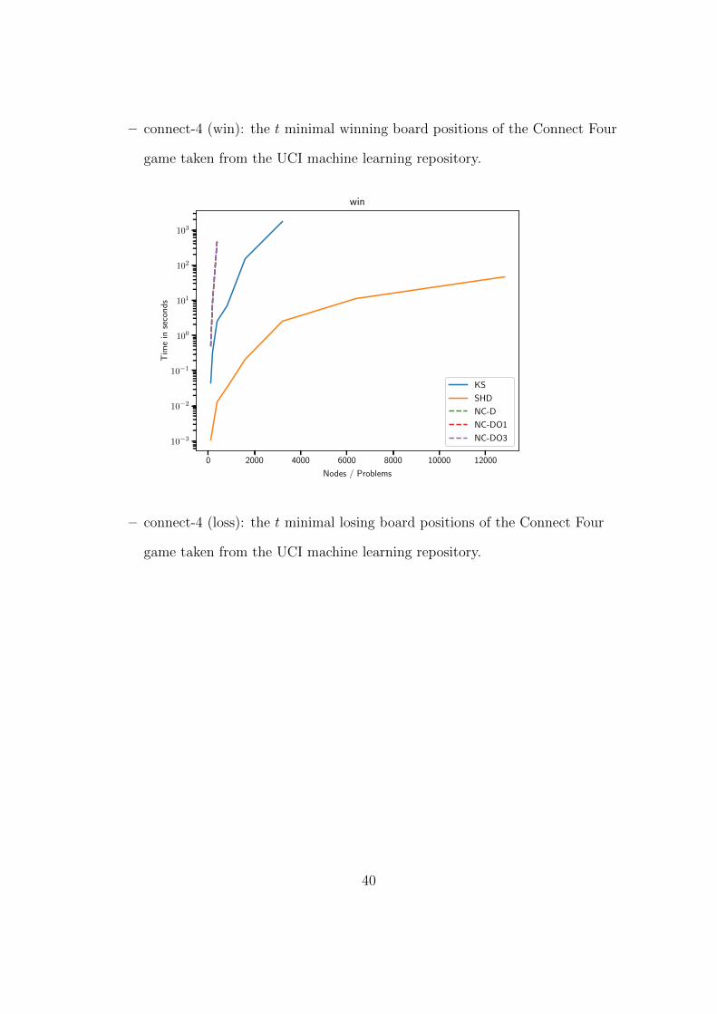
– connect-4 (win): the t minimal winning board positions of the Connect Four

game taken from the UCI machine learning repository.

0 2000 4000 6000 8000 10000 12000

Nodes / Problems

10−3

10−2

10−1

100

101

102

103

Tim

ein

seconds

win

KS

SHD

NC-D

NC-DO1

NC-DO3

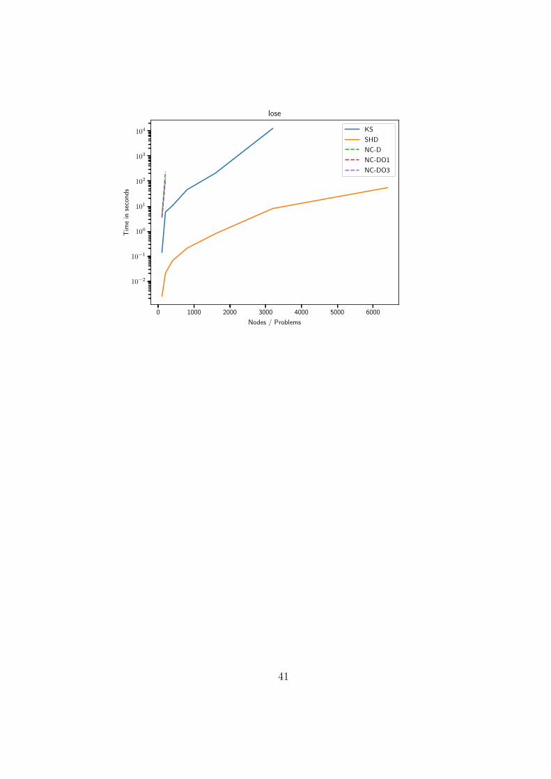
– connect-4 (loss): the t minimal losing board positions of the Connect Four

game taken from the UCI machine learning repository.

40

0 1000 2000 3000 4000 5000 6000

Nodes / Problems

10−2

10−1

100

101

102

103

104Tim

ein

seconds

lose

KS

SHD

NC-D

NC-DO1

NC-DO3

41

CHAPTER X

CONCLUSIONS AND FUTURE DIRECTIONS

This paper has now demonstrated a dynamic polynomial-space,

exponential-time (NC-D) iterative solution to the hypergraph transversal

problem. The mechanics of IntersectCMTWithEdge (Algorithm 12) and

ProcessNewCMT (Algorithm 17) were originally described in a recursive

solution Khachiyan et al. [2006]. Similar to the previous recursive solution, all

of the 2|Gamma| cross-product children need to be enumerated and each child still

needs to inspect the previous set of transversals to determine if it is appropriate to

add it as a new transversal.

Improvements Over Previous Solutions

Improvements over previous solutions were in several areas. Odometers

replaced both the set and bit vector representation in the KS implementation.

Odometers are used to represent hyperedges, indices, generalized variables,

transversals and as exponential enumeration variable counters. Lists of odometers

represented compact minimal transversals and the processing of odometers

in functions. Lists of lists of odometers represented the entire solution to a

exponential problem where the polynomial number of polynomial encodings

contains exactly all of the solutions. Each CMT takes exponential time to

enumerate all of its transversals. The efficient storage is of particular interest

as ProcessNewCMT (Algorithm 17) shortcuts an exponential number of

comparisons by leveraging DoesAHitAll (Algorithm 2) to determine if a child

is appropriate to add to the next generation of CMT s.

42

Both versions must consider the previous transversals minus its parent,

but the recursive version did not have a mechanism to store the previous list of

transversals. The algorithm had to generate each one by using recursion and

a complex call stack to store the states. Consider the recursive solution that

enumerates each of the previous transversals without storing them. This leads

to exponential time to recompute previous transversals and memory use grows

proportionally to the number of hyperedges.

Parallelization

There are multiple components of the NC-D algorithm that can be distributed

for performance gains that scale to the number of computation units available.

Consider that, like all dynamic algorithms, the next set of solutions must be

computed from the current set of solutions. A three-staged pipeline could maximize

the throughput of available compute nodes for this algorithm.

The first parallel stage is that each CMT has 2|Gamma| potential children and

each one can be computed given a hyperedge, in fact every CMT can generate all

of its potential children CMT ’s independently. Consider N compute nodes each

working with a specific CMT and hyperedge to fill a pipeline of children CMT s

work items.

The transversal generation, testing, and compaction can happen in parallel in

multiple places. The generation of each transversal from each CMT can be done

independently. The testing of each new potential CMT against the previous CMT

can be done independently. The condensing of the transversals into the next list of

CMT can be done in parallel with memory locking mechanisms.

43

NC-DO2 Optimization

A further optimization on ProcessNewCMT1 (Algorithm 24) is to replace

the call to RemoveHittingTransversals (Algorithm 22) with a call to a new

optimized version. Enumeration of all transversals of a CMT is not necessary.

Enumeration of only the transversals that hit is required. This can be calculated

and directly enumerated using the previous exponential extraction of all gamma

types. Version NC-DO1 does the preliminary check to see if the enumeration of

transversals is even required. This only eliminates the need to enumerate them if it

is not possible to hit them.

The second optimization is to generate only the correct sub-transversals of

a CMT that need to be considered. As previously noticed, only the intersections

of the current CMT and the Unionize (Algorithm 26) of the previous CMT

need be considered. Interestingly, the IntersectCMTWithEdge (Algorithm

12) function provides the exact segmented results that need to be considered. All

the items in the Beta and Gamma lists can be iterated in the same exponential

method. An iterator that winds through each generated CMT beta and gamma

nodes constructing the sub-transversal that satisfies DoesAHitAll (Algorithm 2)

needs to discard the generated item. As such, each non-discarded item needs to be

collected in a local list of CMT to condense down the exponential non-hitting sets.

The implementing of this methodology is left open for future work.

Advanced Algorithm Applications

The encoded NC-DO3 output can be analyzed without passing the encoding

to an exponential decoder. Simple analysis such as deriving the number of

44

transversals a node participates in is polynomial in the encoded output. Further

analysis of these encodings can benefit clustering.

The first step to the enumeration of objectively better minimal transversals is

first traversing only the minimal traversals in an efficient way Boros et al. [2003].

A simple example is using the number of transversals a node participates in to

identify clusters Bailey et al. [2003].

CondenseMinimalTransversals (Algorithm 20) is highly inefficient in

both time and memory. A tree structure as an intermediate representation instead

of CMT can represent the same transversals program using less memory. All new

interactions of edges with tree representations will need to be derived in the same

manner as the CMT .

45

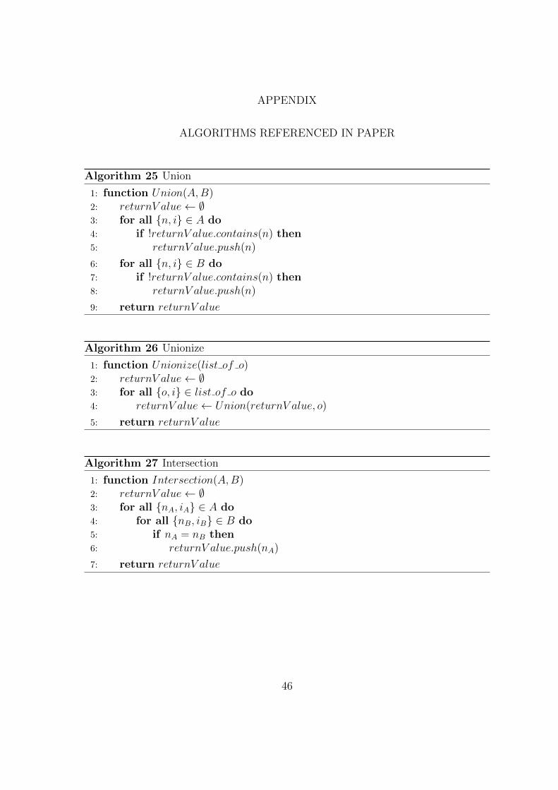
APPENDIX

ALGORITHMS REFERENCED IN PAPER

Algorithm 25 Union

1: function Union(A,B)2: returnV alue← ∅3: for all {n, i} ∈ A do4: if !returnV alue.contains(n) then5: returnV alue.push(n)

6: for all {n, i} ∈ B do7: if !returnV alue.contains(n) then8: returnV alue.push(n)

9: return returnV alue

Algorithm 26 Unionize

1: function Unionize(list of o)2: returnV alue← ∅3: for all {o, i} ∈ list of o do4: returnV alue← Union(returnV alue, o)

5: return returnV alue

Algorithm 27 Intersection

1: function Intersection(A,B)2: returnV alue← ∅3: for all {nA, iA} ∈ A do4: for all {nB, iB} ∈ B do5: if nA = nB then6: returnV alue.push(nA)

7: return returnV alue

46

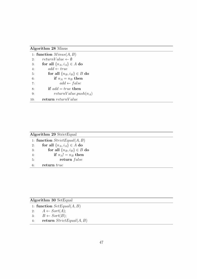
Algorithm 28 Minus

1: function Minus(A,B)2: returnV alue← ∅3: for all {nA, iA} ∈ A do4: add← true5: for all {nB, iB} ∈ B do6: if nA = nB then7: add← false

8: if add = true then9: returnV alue.push(nA)

10: return returnV alue

Algorithm 29 StrictEqual

1: function StrictEqual(A,B)2: for all {nA, iA} ∈ A do3: for all {nB, iB} ∈ B do4: if nA! = nB then5: return false

6: return true

Algorithm 30 SetEqual

1: function SetEqual(A,B)2: A← Sort(A);3: B ← Sort(B);4: return StrictEqual(A,B)

47

REFERENCES CITED

Thomas Eiter. On transveral hypergraph computation and deciding hypergraphsaturation. na, 1991.

Thomas Eiter and Georg Gottlob. Identifying the minimal transversals of ahypergraph and related problems. SIAM Journal on Computing, 24(6):1278–1304, 1995.

Raymond Reiter. A theory of diagnosis from first principles. Artificial intelligence,32(1):57–95, 1987.

Johan De Kleer and Brian C Williams. Diagnosing multiple faults. Artificialintelligence, 32(1):97–130, 1987.

Dimitris J Kavvadias and Elias C Stavropoulos. An efficient algorithm for thetransversal hypergraph generation. J. Graph Algorithms Appl., 9(2):239–264,2005.

Phillip P. Fuchs. Permutation Odometers. www.quickperm.org/odometers.php,2016.

Celine Hebert, Alain Bretto, and Bruno Cremilleux. A data mining formalizationto improve hypergraph minimal transversal computation. FundamentaInformaticae, 80(4):415–433, 2007.

Guozhu Dong and Jinyan Li. Mining border descriptions of emerging patterns fromdataset pairs. Knowledge and Information Systems, 8(2):178–202, 2005.

Dimitris J Kavvadias and Elias C Stavropoulos. Evaluation of an algorithm for thetransversal hypergraph problem. In International Workshop on AlgorithmEngineering, pages 72–84. Springer, 1999.

Leonid Khachiyan, Endre Boros, Khaled Elbassioni, and Vladimir Gurvich. Anefficient implementation of a quasi-polynomial algorithm for generatinghypergraph transversals and its application in joint generation. DiscreteApplied Mathematics, 154(16):2350–2372, 2006.

Endre Boros, K Elbassioni, Vladimir Gurvich, and Leonid Khachiyan. An efficientimplementation of a quasi-polynomial algorithm for generating hypergraphtransversals. In European Symposium on Algorithms, pages 556–567. Springer,2003.

48

James Bailey, Thomas Manoukian, and Kotagiri Ramamohanarao. A fast algorithmfor computing hypergraph transversals and its application in mining emergingpatterns. In Data Mining, 2003. ICDM 2003. Third IEEE InternationalConference on, pages 485–488. IEEE, 2003.

49