The five existing large segmented mirror tele-scopes—the two Keck telescopes [1], the Hobby–Eberly Telescope (HET) [2], the Southern AfricanLarge Telescope (SALT) [3], and the Gran TelescopioCanarias (GTC) [4]—all stabilize their segmentedprimary mirrors with active control systems of edgesensors and segment position actuators so that theyfunction as single monolithic pieces of glass. Thesame is true for the giant segmented telescopes cur-rently in the design stage [5–7]. These controlsystems range in size from those of the Keck tele-scopes and the GTC, each of which has 168 sensorsand 108 actuators to control their 36 segments, to atleast as large as the Thirty Meter Telescope (TMT),with 2772 sensors and 1476 actuators to control its492 segments. Although the sensing is local, the
control algorithm in each of these systems is global.This gives the mirror great stability, but it alsomeans that the effects of a single malfunctioning sen-sor will be propagated through the entire mirror,with potentially serious consequences for the overallimage quality of the telescope.
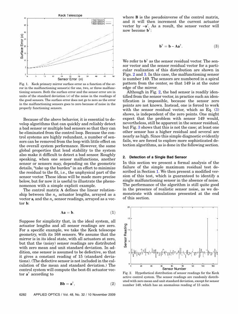
The degradation of image quality is illustrated inFig. 1 for the Keck telescope control system. Thisshows the primary mirror surface error, in units ofthe sensor noise σ, as a function of the error (assumedconstant) in one, two, or three sensors, also expressedin units of the sensor noise. (The surface error doesnot go to zero as the error in the malfunctioning sen-sor goes to zero because of the noise in the properlyfunctioning sensors.) Thus, for example, two mal-functioning sensors each with errors of 50σ (a rela-tively modest error, since the sensor noise σ is lessthan 10nm) will more than quadruple the primarymirror surface error. (For details of the calculationunderlying this figure, see Section 4.)
Because of the above behavior, it is essential to de-velop algorithms that can quickly and reliably detecta bad sensor or multiple bad sensors so that they canbe eliminated from the control loop. Because the con-trol systems are highly redundant, a number of sen-sors can be removed from the loop with little effect onthe overall system performance. However, the sameglobal properties that lend stability to the systemalso make it difficult to detect a bad sensor. Roughlyspeaking, when one sensor malfunctions, anothersensor or sensors may, depending on the geometricdetails, “take up the burden” in an effort to minimizethe residual to the fit, i.e., the unphysical part of thesensor vector. These ideas will be made more precisebelow, but for now it is useful to illustrate the pheno-nomenon with a simple explicit example.The control matrix A defines the linear relation-
ship between the na actuator lengths, arrayed as avector a, and the ns sensor readings, arrayed as a vec-tor b:
Aa ¼ b: ð1Þ
Suppose for simplicity that, in the ideal system, allactuator lengths and all sensor readings are zero.For a specific example, we take the Keck telescopegeometry, with its 168 sensors. We assume that themirror is in its ideal state, with all actuators at zero,but that the (noisy) sensor readings are distributedwith zero mean and unit standard deviation. In ad-dition, one sensor is assumed to be defective, so thatit gives a constant reading of 15 (standard devia-tions). (The defective sensor is not included in the cal-culation of the mean and standard deviation.) Thecontrol system will compute the best-fit actuator vec-tor a† according to
Bb ¼ a†; ð2Þ
where B is the pseudoinverse of the control matrix,and it will then increment the current actuatorvector by −a†. As a result, the sensor vector willnow become b†:
b† ¼ b − Aa†: ð3Þ
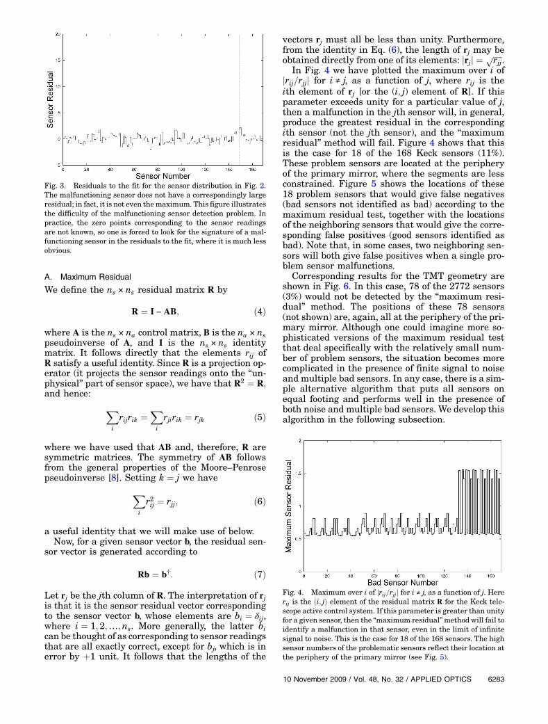
We refer to b† as the sensor residual vector. The sen-sor vector and the sensor residual vector for a parti-cular realization of this distribution are shown inFigs. 2 and 3. In this case, the malfunctioning sensoris number 149. The sensors are numbered in a spiralpattern from the center, so that 149 is at the outeredge of the mirror.
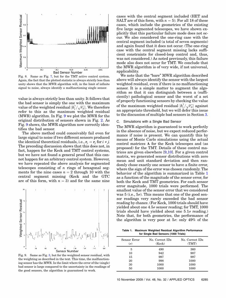
Although in Fig. 2, the bad sensor is readily iden-tified from the sensor vector, in practice such an iden-tification is impossible, because the sensor zeropoints are not known. Instead, one is forced to workwith the sensor residual vector, which as Eq. (3)shows, is independent of the zero points. One mightexpect that the problem with sensor 149 would,nevertheless, still be apparent in the sensor residual,but Fig. 3 shows that this is not the case; at least oneother sensor has a higher residual and several arenearly as high. Since this simple diagnostic evidentlyfails, we are forced to explore more sophisticated de-tection algorithms, as is done in the following section.
2. Detection of a Single Bad Sensor
In this section we present a formal analysis of thefailure of the simple maximum residual test de-scribed in Section 1. We then present a modified ver-sion of this test, which is guaranteed to identify asingle malfunctioning sensor in the absence of noise.The performance of the algorithm is still quite goodin the presence of realistic sensor noise, as we de-monstrate with simulations presented at the endof this section.
Fig. 1. Keck primary mirror surface error as a function of the er-ror in the malfunctioning sensor(s) for one, two, or three malfunc-tioning sensors. Both the surface error and the sensor error are inunits of the standard deviation (σ) of the noise in the readings ofthe good sensors. The surface error does not go to zero as the errorin the malfunctioning sensors goes to zero because of noise in theproperly functioning sensors.
Fig. 2. Hypothetical distribution of sensor readings for the Keckactive control system. The sensor readings are randomly distrib-uted with zeromean and unit standard deviation, except for sensornumber 149, which has an anomalous reading of 15 units.
where A is the ns × na control matrix, B is the na × nspseudoinverse of A, and I is the ns × ns identitymatrix. It follows directly that the elements rij ofR satisfy a useful identity. Since R is a projection op-erator (it projects the sensor readings onto the “un-physical” part of sensor space), we have that R2 ¼ R;and hence:
X
i
rijrik ¼X
i
rjirik ¼ rjk ð5Þ
where we have used that AB and, therefore, R aresymmetric matrices. The symmetry of AB followsfrom the general properties of the Moore–Penrosepseudoinverse [8]. Setting k ¼ j we have
X
i
r2ij ¼ rjj; ð6Þ
a useful identity that we will make use of below.Now, for a given sensor vector b, the residual sen-
sor vector is generated according to
Rb ¼ b†: ð7Þ
Let rj be the jth column of R. The interpretation of rjis that it is the sensor residual vector correspondingto the sensor vector b, whose elements are bi ¼ δij,where i ¼ 1; 2;…;ns. More generally, the latter bican be thought of as corresponding to sensor readingsthat are all exactly correct, except for bj, which is inerror by þ1 unit. It follows that the lengths of the
vectors rj must all be less than unity. Furthermore,from the identity in Eq. (6), the length of rj may beobtained directly from one of its elements: jrjj ¼ ffiffiffiffiffirjj
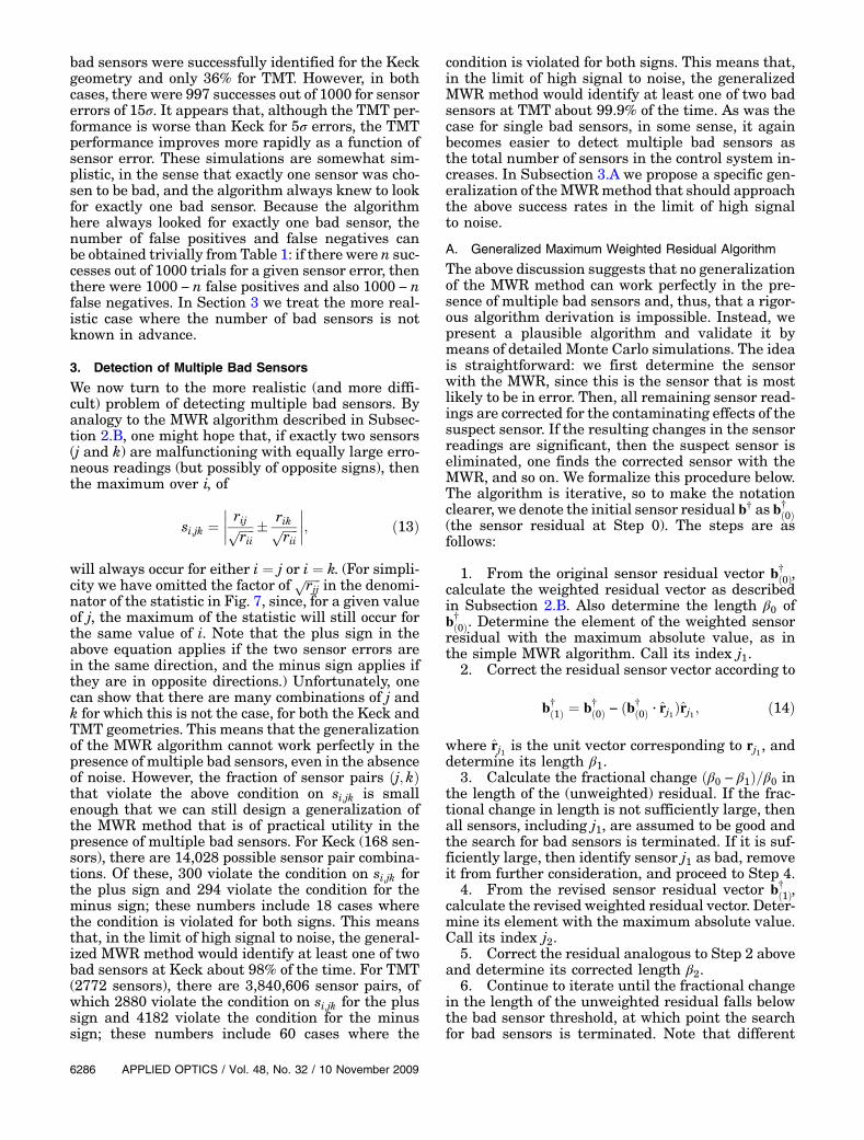
p .In Fig. 4 we have plotted the maximum over i of
jrij=rjjj for i ≠ j, as a function of j, where rij is theith element of rj [or the (i; j) element of R]. If thisparameter exceeds unity for a particular value of j,then a malfunction in the jth sensor will, in general,produce the greatest residual in the correspondingith sensor (not the jth sensor), and the “maximumresidual” method will fail. Figure 4 shows that thisis the case for 18 of the 168 Keck sensors (11%).These problem sensors are located at the peripheryof the primary mirror, where the segments are lessconstrained. Figure 5 shows the locations of these18 problem sensors that would give false negatives(bad sensors not identified as bad) according to themaximum residual test, together with the locationsof the neighboring sensors that would give the corre-sponding false positives (good sensors identified asbad). Note that, in some cases, two neighboring sen-sors will both give false positives when a single pro-blem sensor malfunctions.
Corresponding results for the TMT geometry areshown in Fig. 6. In this case, 78 of the 2772 sensors(3%) would not be detected by the “maximum resi-dual” method. The positions of these 78 sensors(not shown) are, again, all at the periphery of the pri-mary mirror. Although one could imagine more so-phisticated versions of the maximum residual testthat deal specifically with the relatively small num-ber of problem sensors, the situation becomes morecomplicated in the presence of finite signal to noiseand multiple bad sensors. In any case, there is a sim-ple alternative algorithm that puts all sensors onequal footing and performs well in the presence ofboth noise and multiple bad sensors. We develop thisalgorithm in the following subsection.
Fig. 3. Residuals to the fit for the sensor distribution in Fig. 2.The malfunctioning sensor does not have a correspondingly largeresidual; in fact, it is not even themaximum. This figure illustratesthe difficulty of the malfunctioning sensor detection problem. Inpractice, the zero points corresponding to the sensor readingsare not known, so one is forced to look for the signature of a mal-functioning sensor in the residuals to the fit, where it is much lessobvious.
Fig. 4. Maximum over i of jrij=rjjj for i ≠ j, as a function of j. Hererij is the ði; jÞ element of the residual matrix R for the Keck tele-scope active control system. If this parameter is greater than unityfor a given sensor, then the “maximum residual”method will fail toidentify a malfunction in that sensor, even in the limit of infinitesignal to noise. This is the case for 18 of the 168 sensors. The highsensor numbers of the problematic sensors reflect their location atthe periphery of the primary mirror (see Fig. 5).
Suppose we know that exactly one of the ns sensors isreading incorrectly and we want to identify whichone it is by analyzing the elements of the sensor re-sidual vector b†. It is convenient for the moment tonormalize this residual so that it becomes the unitvector b̂†. Conceptually, what we want to do is to com-pare b̂† to the “library” of theoretical residual unitvectors ri=
ffiffiffiffiffirii
p, corresponding to all possible sensors,
and look for the best match. In the absence of noise,
or in the limit of high signal to noise, the index j of thebad sensor must be that value of i that produces anexact match. We can formalize this procedure as fol-lows. We want to find that value of i that maximizesthe scalar product:
pi ¼ b† · ri=ffiffiffiffiffirii
p; ð8Þ
where we have skipped the unnecessary normaliza-tion of b†. The dot product pi can be simplified asfollows:
pi ¼X
j
rjib†j =
ffiffiffiffiffirii
p; ð9Þ
¼X
jk
rjirjkbk=ffiffiffiffiffirii
p; ð10Þ
¼X
k
rikbk=ffiffiffiffiffirii
p; ð11Þ
¼ b†i =ffiffiffiffiffirii
p; ð12Þ
where we have, again, made use of the symmetry ofRand of the fact that R2 ¼ R.
Now, if we take b† to be the sensor residual corre-sponding to a unit error in sensor j (and with all othersensors reading correctly), we have b†i ¼ rij and,therefore, in this case pi ¼ rij=
ffiffiffiffiffirii
p. In Figs. 7 and 8
we have plotted the maximum value of the ratiojrij= ffiffiffiffiffiffiffiffiffi
riirjjp j for i ≠ j as a function of j for the Keck
and TMT control systems, respectively. Here j is tobe interpreted as the index of the (single) bad sensor.For i ¼ j, this ratio clearly takes on the value unity.The figures show that, with the restriction i ≠ j, the
Fig. 5. Solid circles show the positions of the 18 sensors on theKeck telescope that would give false negatives according to themaximum residual test. The nearest-neighbor open circles givethe positions of the sensors that would give the corresponding falsepositives. Note that, in some cases, two different nearest neighborsboth give false positives. (The map is not quite symmetrical be-cause the distributions of the sensors and actuators (not shown)have different symmetries.)
Fig. 6. Same as Fig. 4, but for the TMT active control system. Inthis case, the “maximum residual” method fails for 78 of 2772 sen-sors for which the plotted statistic exceeds unity.
Fig. 7. Same as Fig. 4, but now the plotted function is the max-imum over i of the ratio jrij= ffiffiffiffiffiffiffiffiffiffiriirjj
p j for i ≠ j, as a function of j, againfor the Keck telescope. Note the different denominator comparedto Fig. 4. In the current figure, this ratio never exceeds unity forany sensor. As a result, this MWR algorithm will, in the limit ofinfinite signal to noise, always identify a single malfunctioningsensor.
value is always strictly less than unity. It follows thatthe bad sensor is simply the one with the maximumvalue of the weighted residual jb†i =
ffiffiffiffiffirii
p j. We thereforerefer to this as the maximum weighted residual(MWR) algorithm. In Fig. 9 we plot the MWR for theoriginal distribution of sensors shown in Fig. 2. AsFig. 9 shows, the MWR algorithm now correctly iden-tifies the bad sensor.The above method could conceivably fail even for
large signal to noise if two different sensors producedthe identical theoretical residuals, i.e., ri ¼ rj for i ≠ j.The preceding discussion shows that this does not, infact, happen for the Keck and TMT control systems,but we have not found a general proof that this can-not happen for an arbitrary control system. However,we have repeated the above analysis for segmentedtelescopes consisting of n rings of hexagonal seg-ments for the nine cases n ¼ 2 through 10 with thecentral segment missing (Keck and the GTCare of this form, with n ¼ 3) and for the same nine
cases with the central segment included (HET andSALT are of this form, with n ¼ 5). For all 18 of thesecases, which include the geometries of the existingfive large segmented telescopes, we have shown ex-plicitly that this particular failure mode does not oc-cur. We also considered the one-ring case with thecentral segment included (a total of seven segments)and again found that it does not occur. (The one-ringcase with the central segment missing lacks suffi-cient constraints for closed-loop control and, thus,was not considered.) As noted previously, this failuremode also does not occur for TMT. We conclude thatthe MWR algorithm is of very wide, if not universal,applicability.
We note that the “bare” MWR algorithm describedabove will always identify the sensor with the largestweighted residual, even if there is no malfunctioningsensor. It is a simple matter to augment the algo-rithm so that it can distinguish between a (suffi-ciently) pathological sensor and the worst of a setof properly functioning sensors by checking the valueof the maximum weighted residual jb†i =
ffiffiffiffiffirii
p j againstan appropriate threshold, but we will defer this issueto the discussion of multiple bad sensors in Section 3.
C. Simulations with a Single Bad Sensor
The MWR algorithm is guaranteed to work perfectlyin the absence of noise, but we expect reduced perfor-mance if noise is present. We can quantify this bymeans of Monte Carlo simulations using the actualcontrol matrices A for the Keck telescopes and (asproposed) for the TMT. Details of these control ma-trices are given elsewhere [9,10]. For a given controlmatrix, we generated sensor distributions with zeromean and unit standard deviation and then ran-domly chose exactly one sensor to have a finite error,where the sign of the error was chosen randomly. Thebehavior of the algorithm is summarized in Table 1as a function of the magnitude of the sensor error, forboth the Keck and TMT geometries. For each sensorerror magnitude, 1000 trials were performed. Thesmallest value of the sensor error that we consideredwas 5 (i.e., 5σ). This means that one of the good sen-sor readings very rarely exceeded the bad sensorreading by chance. (For Keck, 1000 trials should haveyielded about one 4:5σ sensor reading; for TMT, 1000trials should have yielded about one 5:1σ reading.)Note that, for both geometries, the performance ofthe algorithm is very poor at 5σ: only 49% of the
Fig. 8. Same as Fig. 7, but for the TMT active control system.Again, the fact that the plotted statistic is always strictly less thanunity shows that the MWR algorithm will, in the limit of infinitesignal to noise, always identify a malfunctioning single sensor.
Fig. 9. Same as Fig. 3, but for the weighted sensor residual, withthe weighting as described in the text. This time, the malfunction-ing sensor has theMWR. In the limit where the error of the (single)bad sensor is large compared to the uncertainty in the readings ofthe good sensors, the algorithm is guaranteed to work.
Table 1. Maximum Weighted Residual Algorithm Performancefor Single Bad Sensors (1000 Trials)
bad sensors were successfully identified for the Keckgeometry and only 36% for TMT. However, in bothcases, there were 997 successes out of 1000 for sensorerrors of 15σ. It appears that, although the TMT per-formance is worse than Keck for 5σ errors, the TMTperformance improves more rapidly as a function ofsensor error. These simulations are somewhat sim-plistic, in the sense that exactly one sensor was cho-sen to be bad, and the algorithm always knew to lookfor exactly one bad sensor. Because the algorithmhere always looked for exactly one bad sensor, thenumber of false positives and false negatives canbe obtained trivially from Table 1: if there were n suc-cesses out of 1000 trials for a given sensor error, thenthere were 1000 − n false positives and also 1000 − nfalse negatives. In Section 3 we treat the more real-istic case where the number of bad sensors is notknown in advance.
3. Detection of Multiple Bad Sensors
We now turn to the more realistic (and more diffi-cult) problem of detecting multiple bad sensors. Byanalogy to the MWR algorithm described in Subsec-tion 2.B, one might hope that, if exactly two sensors(j and k) are malfunctioning with equally large erro-neous readings (but possibly of opposite signs), thenthe maximum over i, of
si;jk ¼����rijffiffiffiffiffirii
p � rikffiffiffiffiffirii
p����; ð13Þ
will always occur for either i ¼ j or i ¼ k. (For simpli-city we have omitted the factor of ffiffiffiffiffi
rjjp in the denomi-
nator of the statistic in Fig. 7, since, for a given valueof j, the maximum of the statistic will still occur forthe same value of i. Note that the plus sign in theabove equation applies if the two sensor errors arein the same direction, and the minus sign applies ifthey are in opposite directions.) Unfortunately, onecan show that there are many combinations of j andk for which this is not the case, for both the Keck andTMT geometries. This means that the generalizationof the MWR algorithm cannot work perfectly in thepresence of multiple bad sensors, even in the absenceof noise. However, the fraction of sensor pairs ðj; kÞthat violate the above condition on si;jk is smallenough that we can still design a generalization ofthe MWR method that is of practical utility in thepresence of multiple bad sensors. For Keck (168 sen-sors), there are 14,028 possible sensor pair combina-tions. Of these, 300 violate the condition on si;jk forthe plus sign and 294 violate the condition for theminus sign; these numbers include 18 cases wherethe condition is violated for both signs. This meansthat, in the limit of high signal to noise, the general-ized MWR method would identify at least one of twobad sensors at Keck about 98% of the time. For TMT(2772 sensors), there are 3,840,606 sensor pairs, ofwhich 2880 violate the condition on si;jk for the plussign and 4182 violate the condition for the minussign; these numbers include 60 cases where the
condition is violated for both signs. This means that,in the limit of high signal to noise, the generalizedMWR method would identify at least one of two badsensors at TMT about 99.9% of the time. As was thecase for single bad sensors, in some sense, it againbecomes easier to detect multiple bad sensors asthe total number of sensors in the control system in-creases. In Subsection 3.A we propose a specific gen-eralization of theMWRmethod that should approachthe above success rates in the limit of high signalto noise.
A. Generalized Maximum Weighted Residual Algorithm
The above discussion suggests that no generalizationof the MWR method can work perfectly in the pre-sence of multiple bad sensors and, thus, that a rigor-ous algorithm derivation is impossible. Instead, wepresent a plausible algorithm and validate it bymeans of detailed Monte Carlo simulations. The ideais straightforward: we first determine the sensorwith the MWR, since this is the sensor that is mostlikely to be in error. Then, all remaining sensor read-ings are corrected for the contaminating effects of thesuspect sensor. If the resulting changes in the sensorreadings are significant, then the suspect sensor iseliminated, one finds the corrected sensor with theMWR, and so on. We formalize this procedure below.The algorithm is iterative, so to make the notationclearer, we denote the initial sensor residual b† as b†ð0Þ(the sensor residual at Step 0). The steps are asfollows:
1. From the original sensor residual vector b†ð0Þ,calculate the weighted residual vector as describedin Subsection 2.B. Also determine the length β0 ofb†ð0Þ. Determine the element of the weighted sensorresidual with the maximum absolute value, as inthe simple MWR algorithm. Call its index j1.
2. Correct the residual sensor vector according to
b†ð1Þ ¼ b†ð0Þ − ðb†ð0Þ · r̂j1Þr̂j1 ; ð14Þ
where r̂j1 is the unit vector corresponding to rj1 , anddetermine its length β1.
3. Calculate the fractional change ðβ0 − β1Þ=β0 inthe length of the (unweighted) residual. If the frac-tional change in length is not sufficiently large, thenall sensors, including j1, are assumed to be good andthe search for bad sensors is terminated. If it is suf-ficiently large, then identify sensor j1 as bad, removeit from further consideration, and proceed to Step 4.
4. From the revised sensor residual vector b†ð1Þ,calculate the revised weighted residual vector. Deter-mine its element with the maximum absolute value.Call its index j2.
5. Correct the residual analogous to Step 2 aboveand determine its corrected length β2.
6. Continue to iterate until the fractional changein the length of the unweighted residual falls belowthe bad sensor threshold, at which point the searchfor bad sensors is terminated. Note that different
values for the threshold can be used in differ-ent steps.
B. Simulations with Multiple Bad Sensors
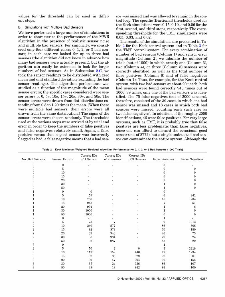
We have performed a large number of simulations inorder to characterize the performance of the MWRalgorithm in the presence of realistic sensor noiseand multiple bad sensors. For simplicity, we consid-ered only four different cases: 0, 1, 2, or 3 bad sen-sors; in each case we looked for up to three badsensors (the algorithm did not know in advance howmany bad sensors were actually present), but the al-gorithm can easily be extended to look for largernumbers of bad sensors. As in Subsection 2.C, wetook the sensor readings to be distributed with zeromean and unit standard deviation (excluding the badsensor readings). The algorithm performance wasstudied as a function of the magnitude of the meansensor errors; the specific cases considered were sen-sor errors of 0, 5σ, 10σ, 15σ, 20σ, 30σ, and 50σ. Thesensor errors were drawn from flat distributions ex-tending from 0.8 to 1.20 times the mean. (When therewere multiple bad sensors, their errors were alldrawn from the same distribution.) The signs of thesensor errors were chosen randomly. The thresholdsused at the various steps were arrived at by trial anderror in order to keep the numbers of false positivesand false negatives relatively small. Again, a falsepositive means that a good sensor was incorrectlyflagged as bad; a false negative means that a bad sen-
sor wasmissed and was allowed to remain in the con-trol loop. The specific (fractional) thresholds used forthe Keck simulations were 0.15, 0.10, and 0.06 for thefirst, second, and third steps, respectively. The corre-sponding thresholds for the TMT simulations were0.05, 0.03, and 0.02.
The results of the simulations are presented in Ta-ble 2 for the Keck control system and in Table 3 forthe TMT control system. For every combination ofnumber of bad sensors (Column 1) and sensor errormagnitude (Column 2), we tabulate the number oftrials (out of 1000) in which exactly one (Column 3),two (Column 4), or three (Column 5) sensors werecorrectly identified, as well as the total number offalse positives (Column 6) and of false negatives(Column 7). Thus, for example, for the Keck controlsystem, with two bad sensors at about 20σ each, bothbad sensors were found correctly 943 times out of1000; 39 times, only one of the bad sensors was iden-tified. The 75 false negatives (out of 2000 sensors),therefore, consisted of the 39 cases in which one badsensor was missed and 18 cases in which both badsensors were missed (counting each such case astwo false negatives). In addition, of the roughly 2000identifications, 46 were false positives. For very largesystems, such as TMT, it is probably true that falsepositives are less problematic than false negatives,since one can afford to discard the occasional goodsensor (out of 2772), but a single undetected bad sen-sor can contaminate the entire system. Although the
Table 2. Keck Maximum Weighted Residual Algorithm Performance for 0, 1, 2, or 3 Bad Sensors (1000 Trials)
No. Bad Sensors Sensor Error σCorrect IDsof 1 Sensor
results in Tables 2 and 3 have not necessarily beenoptimized with respect to the threshold settings(indeed, it is not entirely clear what “optimal”meansin this context), it is interesting to note that, in somecases (e.g., three bad sensors), the detection of badsensors is actually easier for TMT than for Keck,despite the much larger number of sensors in TMT.This counterintuitive result may be due to the factthat, as discussed in Subsection 2.A, edge effectsin the active control system constitute a major com-plication for the detection algorithm, and the largerthe telescope, the smaller the fraction of sensors nearthe periphery.
4. Discussion
For the extremely large telescopes now under devel-opment, detailed quantitative predictions concerningthe performance of the bad sensor detection algo-rithm proposed here will have to await detailedmodeling of the sensor electronic and mechanicalproperties. Nevertheless, we can get at least an ap-proximate idea of how the algorithm will perform bymeans of the following argument.If we start with a perfect telescope, with all actua-
tors equal to zero and properly functioning but noisysensors, then the sensor noise will manifest itself asactuator errors a† [see Eq. (2)], which are very nearlyequal in an rms sense to the primary mirror surfaceerror. Therefore, for each sensor vector b in the abovesimulations, we calculate a†, as in Eq. (2), and the
rms value of the elements of a† constitutes (or at leastapproximates) the rms surface error. This surface er-ror is plotted for TMTas a function of the error in themalfunctioning sensor(s) in Fig. 10. The correspond-ing plot for Keck was presented in Section 1 (Fig. 1).First consider the plot for Keck. The fact that it was
Table 3. Thirty Meter Telescope Maximum Weighted Residual Algorithm Performance for 0, 1, 2, or 3 Bad Sensors (1000 Trials)
No. Bad Sensors Sensor Error σCorrect IDsof 1 Sensor
Fig. 10. TMT primary mirror surface error as a function of theerror in the malfunctioning sensor(s) for one, two, or three mal-functioning sensors. Both the surface error and the sensor errorare in units of the standard deviation (σ) of the noise in the read-ings of the good sensors. Compared to Keck (see Fig. 1), the con-sequences of a given number of bad sensors for TMT are relativelysmaller for small sensor errors and absolutely smaller for largesensor errors. See text for explanation.
difficult in the above simulations to detect sensorswith an error of 5 to 10σ is not as serious as onemighthave thought, because sensor errors of this magni-tude have a relatively small effect on the overall pri-mary mirror surface error. Conversely, sensors witherrors of 30σ or more have a profound effect on sur-face (or wavefront) quality, but they are relativelyeasy to detect. There is an awkward range for Keckcorresponding to sensor errors between 10 and 30σ,where the bad sensors are difficult to detect, but stillhave a serious effect on the telescope wavefront. Onemight deal with this situation in practice by forcingpatterns with large sensor readings into the tele-scope, in a deliberate attempt to make the sensorerrors worse and, therefore, more obvious. For theTMT, things are better for two reasons. First, thefractional increase in the surface error for small sen-sor errors is smaller for the TMT than for Keck be-cause the noise propagation (in the absence of badsensors) is worse for the TMT (see Figs. 1 and 10).Second, the surface error for large sensor errors issmaller for the TMT, in an absolute sense, than itis for Keck, because the errors are distributed overthe larger mirror. The net result is that there is vir-tually no awkward transition region for TMT: sensorerrors that are too small for the algorithm to detectreliably have only a small effect on the wavefront er-ror, and errors that are big enough to have a signifi-cant effect on wavefront are relatively easy to detect.Of course, the problem of malfunctioning sensors is
more serious for larger telescopes in the sense thatthe same mean time between failures (MTBF) persensor will translate into proportionally larger num-bers of failed sensors for larger telescopes. However,if the MTBF can be lengthened proportionally, it isencouraging that the problem of identifying (a givennumber of) malfunctioning sensors in some sense be-comes easier as the telescope becomes larger. In par-ticular, the generalized MWR algorithm described in
this work appears promising for diagnosing andidentifying as many as three (and possibly more) si-multaneously malfunctioning sensors in the primarymirror control system of the TMT.
References1. J. E. Nelson, T. S. Mast, and S. M. Faber, “The design of the
Keck Observatory and Telescope,” Keck Observatory Report90 (W. M. Keck Observatory, Kamuela, Hawaii 1985).
2. J. A. Booth, M. T. Adams, E. S. Barker, F. N. Bash, J. R. Fowler,J. M. Good, G. J. Hill, P. W. Kelton, D. L. Lambert, P. J. Mac-Queen, P. Palunas, L. W. Ramsey, and G. L. Wesley, “TheHobby–Eberly Telescope: performance upgrades, status andplans,” Proc. SPIE 5489, 288–299 (2004).
3. S. Buous, J. Menzies, and H. Gajjar, “SALT segmented pri-mary mirror: commissioning capacitive edge sensing systemand performance comparison with inductive sensor,” Proc.SPIE 7012, 70123G (2008).
4. J. M. Rodriguez-Espinoza, P. Alvarez, and F. Sanchez, “TheGTC, an advanced 10m telescope for the ORM,” Astrophys.Space Sci. 263, 355–360 (1998).
5. J. Nelson and G. H. Sanders, “TMT status report,” Proc. SPIE6267, 626728 (2006).
6. T. Andersen, A. Ardeberg, J. Beckers, R. Flicker, A. Gont-charov, N. C. Jessen, E. Mannery, M. Owner-Petersen, andH. Riewaldt, “The proposed 50m Swedish Extremely LargeTelescope,” in Proceedings of the Backaskog Workshop on Ex-tremely Large Telescopes, T. Andersen, A. Ardeberg, and R.Gilmozzi, eds., Vol. 57 of European Southern ObservatoryConference and Workshop Proceedings (SPIE, 2000),pp. 72–82.
7. R. Gilmozzi and J. Spyromilio, “The 42m European ELT: sta-tus,” Proc. SPIE 7012, 701219 (2008).
8. See, e.g., http://en.wikipedia.org/wiki/Moore‑Penrose_pseudo‑inverse.
9. R. W. Cohen, T. S. Mast, and J. E. Nelson, “Performance of theW. M. Keck Telescope active mirror control system,” Proc.SPIE 2199, 105–116 (1994).
10. G. Chanan, D. G. MacMartin, J. Nelson, and T. Mast, “Controland alignment of segmented-mirror telescopes: matrices,modes, and error propagation,” Appl. Opt. 43, 1223–1232(2004).