57

Algorithmic Trading as a Science
Haksun Li
www.numericalmethod.com

Speaker Profile
Haksun Li, Numerical Method Inc.
Quantitative Trader
Quantitative Analyst
PhD, Computer Science, University of Michigan Ann Arbor
M.S., Financial Mathematics, University of Chicago
B.S., Mathematics, University of Chicago

Definition
Quantitative trading is the systematic execution of trading orders decided by quantitative market models.
It is an arms race to build
more comprehensive and accurate prediction models (mathematics)
more reliable and faster execution platforms (computer science)

Scientific Trading Models
Scientific trading models are supported by logical arguments.
can list out assumptions
can quantify models from assumptions
can deduce properties from models
can test properties
can do iterative improvements
Superstition
Many “quantitative” models are just superstitions supported by fallacies and wishful-thinking.
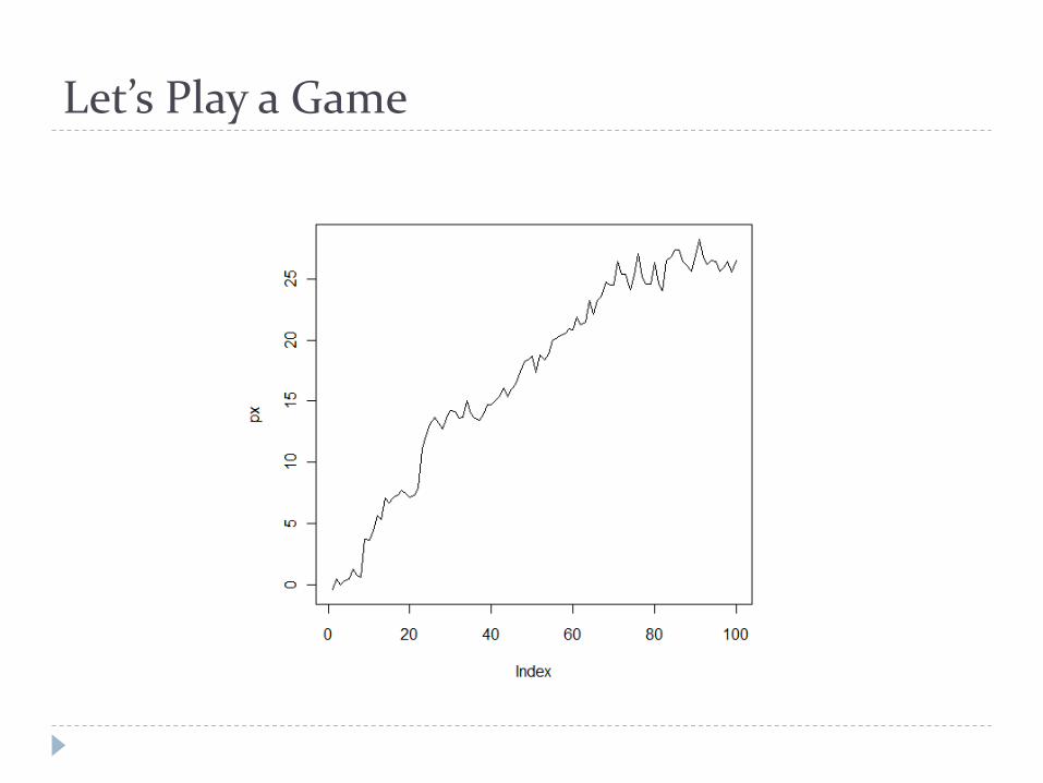
Let’s Play a Game

Impostor Quant. Trader
Decide that this is a bull market
by drawing a line
by (spurious) linear regression
Conclude that
the slope is positive
the t-stat is significant
Long
Take profit at 2 upper sigmas
Stop-loss at 2 lower sigmas

Reality
r = rnorm(100)
px = cumsum(r)
plot(px, type='l')
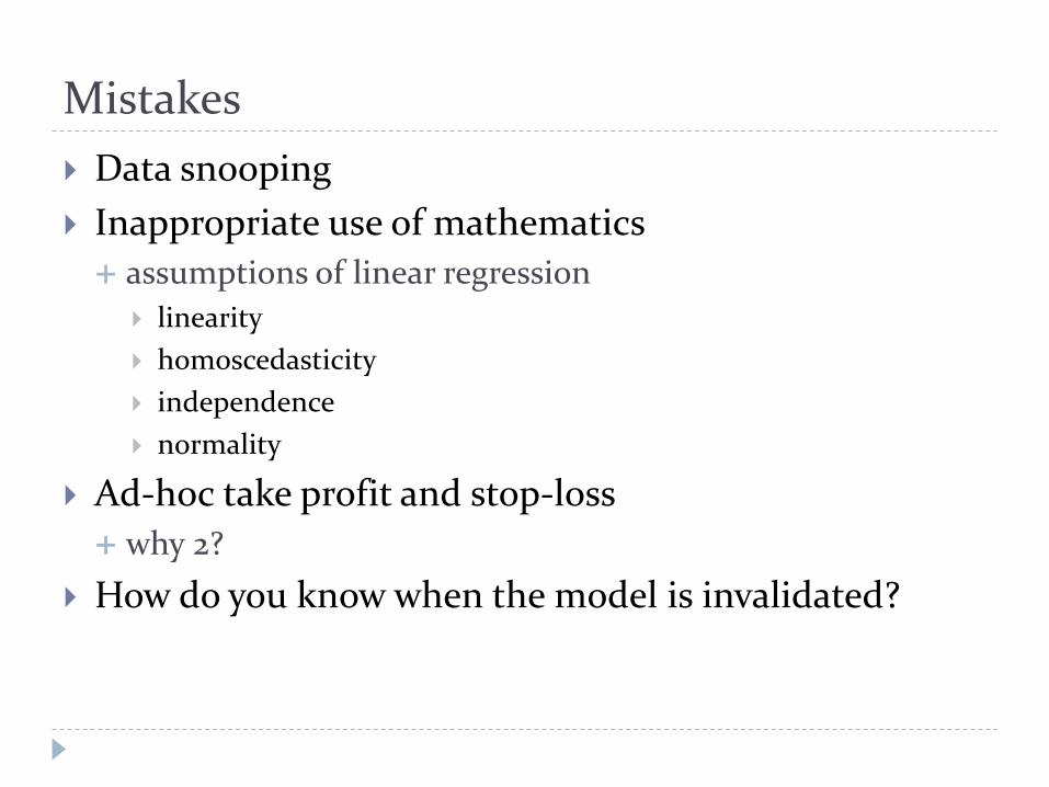
Mistakes
Data snooping
Inappropriate use of mathematics
assumptions of linear regression
linearity
homoscedasticity
independence
normality
Ad-hoc take profit and stop-loss
why 2?
How do you know when the model is invalidated?
Fake Quantitative Models
Assumptions cannot be quantified
No model validation against the current regime
Cannot explain winning and losing trades
Cannot be analyzed (systematically)

Extensions of a Wrong Model
Some traders elaborate on this idea by
using a moving calibration window (e.g., Bands)
using various sorts of moving averages (e.g., MA, WMA, EWMA)
A Scientific Approach
Start with a market insight (hypothesis)
hopefully without peeking at the data
Translate English into mathematics
write down the idea in math formulae
In-sample calibration; out-sample backtesting
Understand why the models work or fail
in terms of model parameters
e.g., unstable parameters, small p-values

MANY Mathematical Tools Available
Markov model
co-integration
stationarity
hypothesis testing
bootstrapping
signal processing, e.g., Kalman filter
returns distribution after news/shocks
time series modeling
The list goes on and on……
A Sample Trading Idea
When the price trends up, we buy.
When the price trends down, we sell.

What is a Trend?

An Upward Trend
More positive returns than negative ones.
Positive returns are persistent.
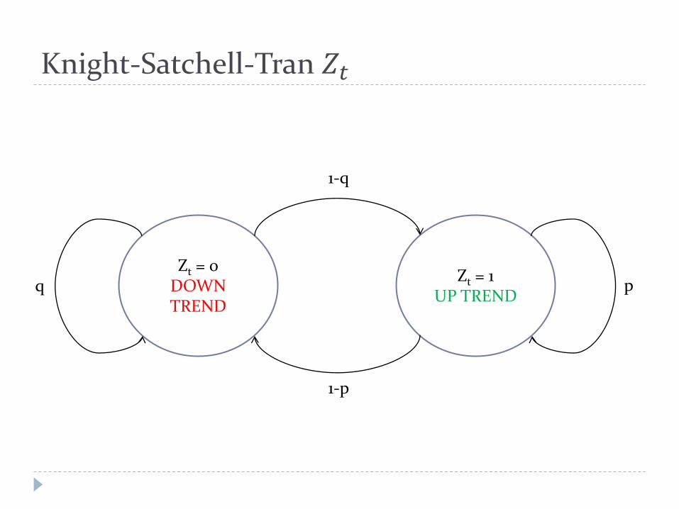
Knight-Satchell-Tran 𝑍𝑡
Zt = 0 DOWN TREND
Zt = 1 UP TREND
q p
1-q
1-p

Knight-Satchell-Tran Process
𝑅𝑡 = 𝜇𝑙 + 𝑍𝑡휀𝑡 − 1 − 𝑍𝑡 𝛿𝑡
𝜇𝑙: long term mean of returns, e.g., 0
휀𝑡, 𝛿𝑡: positive and negative shocks, non-negative, i.i.d
𝑓 𝑥 =𝜆1
𝛼1𝑥𝛼1−1
Γ 𝛼1𝑒−𝜆1𝑥
𝑓𝛿 𝑥 =𝜆2
𝛼2𝑥𝛼2−1
Γ 𝛼2𝑒−𝜆2𝑥

How Signal Do We Use?
Let’s try Moving Average Crossover.

Moving Average Crossover
Two moving averages: slow (𝑛) and fast (𝑚).
Monitor the crossovers.
𝐵𝑡 =1
𝑚 𝑃𝑡−𝑗𝑚−1𝑗=0 −
1
𝑛 𝑃𝑡−𝑗𝑛−1𝑗=0 , 𝑛 > 𝑚
Long when 𝐵𝑡 ≥ 0.
Short when 𝐵𝑡 < 0.
How to choose 𝑛 and 𝑚?
For most traders, it is an art (guess), not a science.
Let’s make our life easier by fixing 𝑚 = 1.
Why?

GMA(n , 1)
𝐵𝑡 ≥ 0 iff 𝑃𝑡 ≥ 𝑃𝑡−𝑗𝑛−1𝑗=0
1
𝑛
𝑅𝑡 ≥ − 𝑛− 𝑗+1
𝑛−1𝑅𝑡−𝑗
𝑛−2𝑗=1 (by taking log)
𝐵𝑡 < 0 iff 𝑃𝑡 < 𝑃𝑡−𝑗𝑛−1𝑗=0
1
𝑛
𝑅𝑡 < − 𝑛− 𝑗+1
𝑛−1𝑅𝑡−𝑗
𝑛−2𝑗=1 (by taking log)

What is 𝑛?
𝑛 = 2
𝑛 = ∞

GMA(2, 1)
Assume the long term mean is 0, 𝜇𝑙 = 0.
𝐵𝑡 ≥ 0 ≡ 𝑅𝑡 ≥ 0 ≡ 𝑍𝑡 = 1
𝐵𝑡 < 0 ≡ 𝑅𝑡 < 0 ≡ 𝑍𝑡 = 0
Naïve MA Trading Rule
Buy when the asset return in the present period is positive.
Sell when the asset return in the present period is negative.
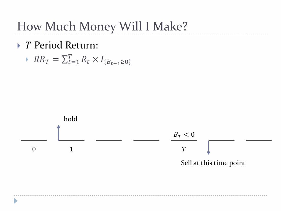
How Much Money Will I Make?
𝑇 Period Return:
𝑅𝑅𝑇 = 𝑅𝑡 × 𝐼 𝐵𝑡−1≥0𝑇𝑡=1
Sell at this time point
𝑇
𝐵𝑇 < 0
0 1
hold

Expected Holding Time
𝑃 𝑁 = 𝑇
= 𝑃 𝐵𝑇 < 0, 𝐵𝑇−1 ≥ 0,… , 𝐵1 ≥ 0, 𝐵0 ≥ 0
= 𝑃 𝑍𝑇 = 0, 𝑍𝑇−1 = 1,… , 𝑍1 = 1, 𝑍0 = 1
= 𝑃 𝑍𝑇 = 0, 𝑍𝑇−1 = 1,… , 𝑍1 = 1|𝑍0 = 1 𝑃 𝑍0 = 1
= Π𝑝𝑇−1 1 − 𝑝 , T ≥1
1 − Π, T=0
Stationary probabilities
Π =1−𝑞
2−𝑝−𝑞

My Returns Distribution (1)
Φ𝑅𝑅𝑇|𝑁=𝑇 𝑠
= E 𝑒𝑖 𝑅𝑡×𝐼 𝐵𝑡−1≥0
𝑇𝑡=1 𝑠
|𝑁 = 𝑇
= E 𝑒𝑖 𝑅𝑡×𝐼 𝐵𝑡−1≥0
𝑇𝑡=1 𝑠
|𝐵𝑇 < 0, 𝐵𝑇−1 ≥ 0,… , 𝐵0 ≥ 0
= E 𝑒 𝑖 𝑅𝑡𝑇𝑡=1 𝑠 |𝑍𝑇 = 0, 𝑍𝑇−1 = 1,… , 𝑍1 = 1
= E 𝑒 𝑖 1+⋯+ 𝑇−1−𝛿𝑇 𝑠
= Φ 𝑇−1 𝑠 Φ𝛿 −𝑠 , T ≥1
Φ𝛿 −𝑠 , T =0
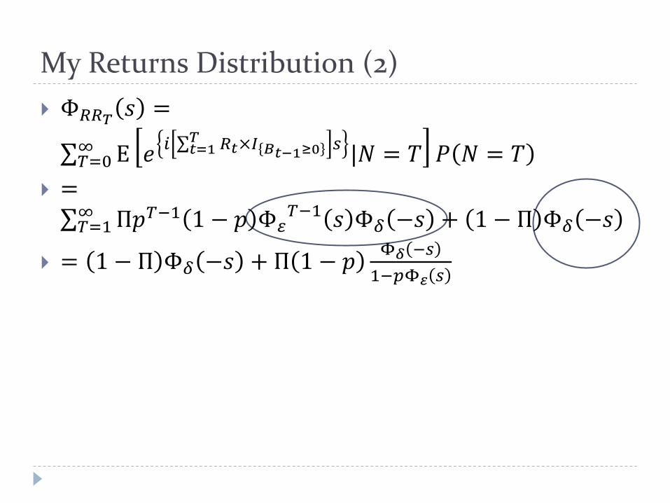
My Returns Distribution (2)
Φ𝑅𝑅𝑇𝑠 =
E 𝑒𝑖 𝑅𝑡×𝐼 𝐵𝑡−1≥0
𝑇𝑡=1 𝑠
|𝑁 = 𝑇 𝑃 𝑁 = 𝑇∞𝑇=0
= Π𝑝𝑇−1 1 − 𝑝 Φ 𝑇−1 𝑠 Φ𝛿 −𝑠∞𝑇=1 + 1 − Π Φ𝛿 −𝑠
= 1 − Π Φ𝛿 −𝑠 + Π 1 − 𝑝Φ𝛿 −𝑠
1−𝑝Φ 𝑠
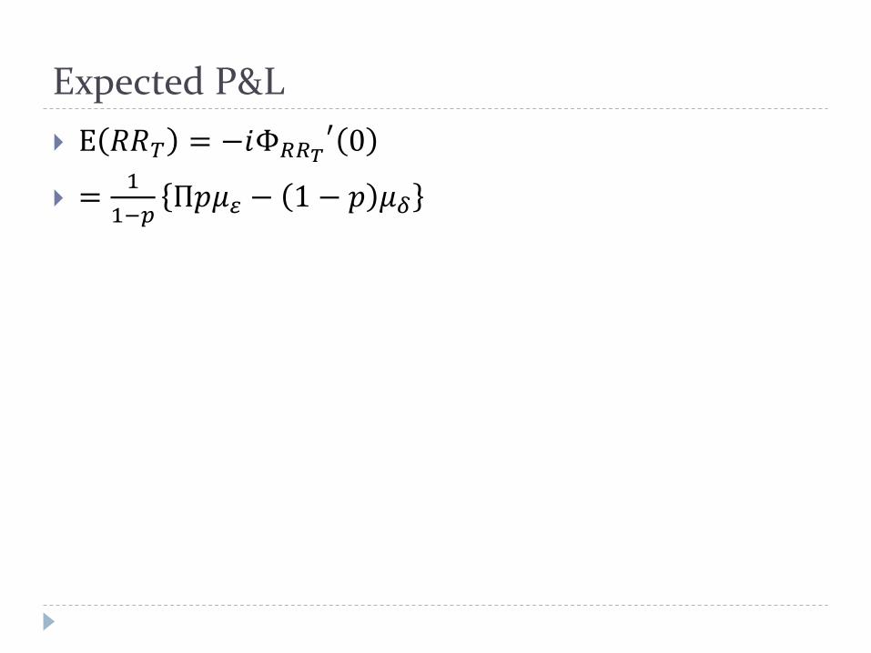
Expected P&L
E 𝑅𝑅𝑇 = −𝑖Φ𝑅𝑅𝑇
′ 0
=1
1−𝑝Π𝑝𝜇 − 1 − 𝑝 𝜇𝛿

When Will My Strategy Make Money?
The expected return is positive when
𝜇 ≥1−𝑝
Π𝑝𝜇𝛿, shock impact
𝜇 ≫ 𝜇𝛿, shock impact
Π𝑝 ≥ 1 − 𝑝, if 𝜇 ≈ 𝜇𝛿, persistence

What About GMA(∞,1)
Repeat the steps above.
E 𝑅𝑅𝑇 = − 1 − 𝑝 1 − Π 𝜇 + 𝜇𝛿

When Will GMA(∞,1) Make Money?

Model Benefits (1)
It makes “predictions” about which regime we are now in.
We quantify how useful the model is by
the parameter sensitivity
the duration we stay in each regime
the state differentiation power

Model Benefits (2)
We can explain winning and losing trades.
Is it because of calibration?
Is it because of state prediction?
We can deduce the model properties.
Are 2 states sufficient?
prediction variance?
We can justify take-profit and stop-loss based on trader utility function.
Backtesting
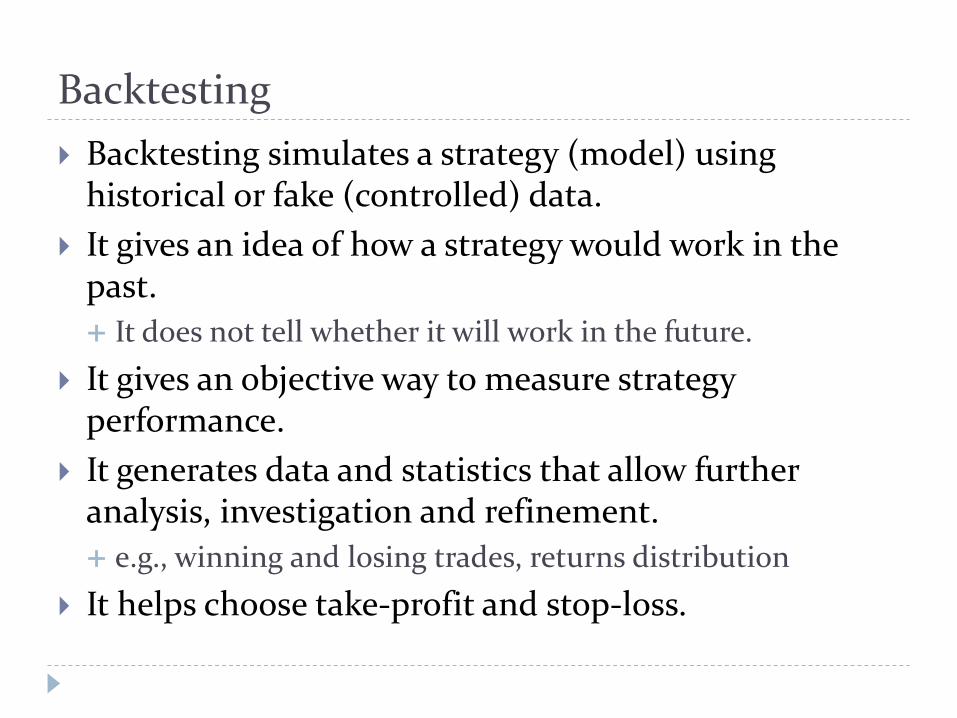
Backtesting simulates a strategy (model) using historical or fake (controlled) data.
It gives an idea of how a strategy would work in the past.
It does not tell whether it will work in the future.
It gives an objective way to measure strategy performance.
It generates data and statistics that allow further analysis, investigation and refinement.
e.g., winning and losing trades, returns distribution
It helps choose take-profit and stop-loss.

Some Performance Statistics
p&l
mean, stdev, corr
Sharpe ratio
confidence intervals
max drawdown
breakeven ratio
biggest winner/loser
breakeven bid/ask
slippage
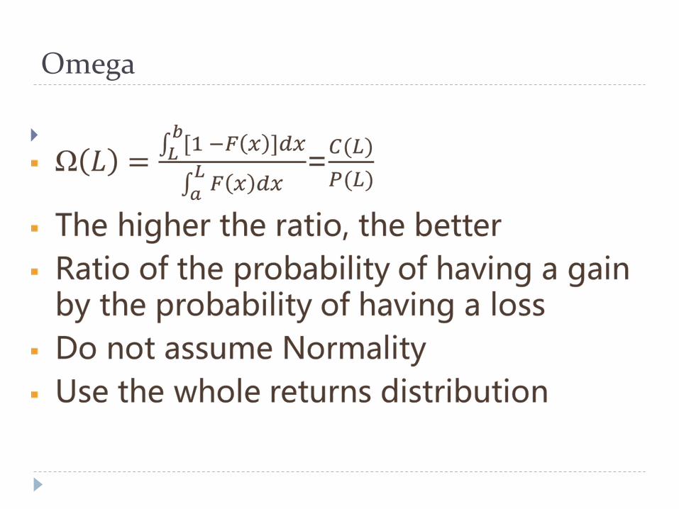
Omega

Performance on MSCI Singapore

Bootstrapping
We observe only one history.
What if the world had evolve different?
Simulate “similar” histories to get confidence interval.
White's reality check (White, H. 2000).

Fake Data
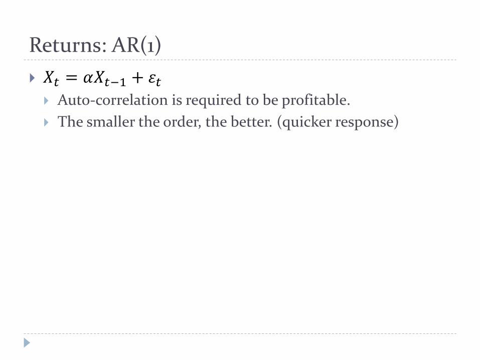
Returns: AR(1)
𝑋𝑡 = 𝛼𝑋𝑡−1 + 휀𝑡
Auto-correlation is required to be profitable.
The smaller the order, the better. (quicker response)

Returns: AR(1)

Returns: ARMA(1, 1)
𝑋𝑡 − 𝜇 − 𝑝 𝑋𝑡−1 − 𝜇 = 휀𝑡 − 𝑞휀𝑡−1
Prices tend to move in one direction (trend) for a period of time and then change in a random and unpredictable fashion.
AR MA
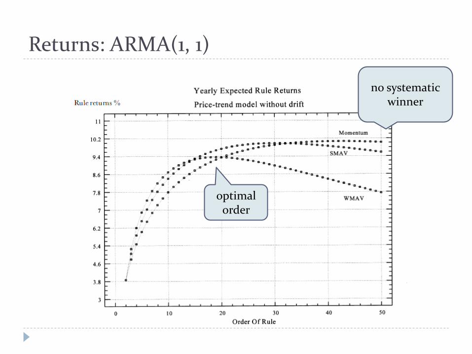
Returns: ARMA(1, 1)
no systematic winner
optimal order

Returns: ARIMA(0, d, 0)
𝛻𝑑 𝑋𝑡 − 𝜇 = 𝑒𝑡
Irregular, erratic, aperiodic cycles.

Returns: ARIMA(0, d, 0)
ARCH + GARCH
The presence of conditional heteroskedasticity, if unrelated to serial dependencies, may be neither a source of profits nor losses for linear rules.
A good Backtester (1)
allow easy strategy programming
allow plug-and-play multiple strategies
simulate using historical data
simulate using fake, artificial data
allow controlled experiments
e.g., bid/ask, execution assumptions, news

A good Backtester (2)
generate standard and user customized statistics
have information other than prices
e.g., macro data, news and announcements
Auto calibration
Sensitivity analysis
Quick

Matlab/R
They are very slow. These scripting languages are interpreted line-by-line. They are not built for parallel computing.
They do not handle a lot of data well. How do you handle two year worth of EUR/USD tick by tick data in Matlab/R?
There is no modern software engineering tools built for Matlab/R. How do you know your code is correct?
The code cannot be debugged easily. Ok. Matlab comes with a toy debugger somewhat better than gdb. It does not compare to NetBeans, Eclipse or IntelliJ IDEA.
Calibration
Most strategies require calibration to update parameters for the current trading regime.
Occam’s razor: the fewer parameters the better.
For strategies that take parameters from the Real line: Nelder-Mead, BFGS
For strategies that take integers: Mixed-integer non-linear programming (branch-and-bound, outer-approximation)

Global Optimization Methods
f

Sensitivity
How much does the performance change for a small change in parameters?
Avoid the optimized parameters merely being statistical artifacts.
A plot of measure vs. d(parameter) is a good visual aid to determine robustness.
We look for plateaus.
Iterative Refinement
Backtesting generates a large amount of statistics and data for model analysis.
We may improve the model by
regress the winning/losing trades with factors
identify, delete/add (in)significant factors
check serial correlation among returns
check model correlations
the list goes on and on……

Implementation
Connectivity to exchanges
e.g., ION, RTS
Platform dependent APIs
Programming languages
Java, C++, C#, VBA, Matlab
Summary
Market understanding gives you an intuition to a trading strategy.
Mathematics is the tool that makes your intuition concrete and precise.
Programming is the skill that turns ideas and equations into reality.


