Algorithms for magnetic tomography - on the role of a ...

Algorithms for magnetic tomography - on the role

of a priori knowledge and constraints

Karl-Heinz Hauer1, Roland Potthast2 and Martin Wannert3

1TomoScience GbR, Major-Hirst-Str. 11 (Innovationscampus), 38442 Wolfsburg,Germany2Department of Mathematics, University of Reading, Whiteknights, PO Box 220,Berkshire, RG6 6AX, UK3Forschungszentrum Julich, Institute of Energy Research - Fuel Cells (IEF-3), 52425Julich, Germany

E-mail: [email protected], [email protected] [email protected]

Abstract. Magnetic tomography investigates the reconstruction of currents fromtheir magnetic fields. Here, we will study a number of projection methods incombination with the Tikhonov regularization for stabilization for the solution ofthe Biot-Savart integral equation Wj = H with the Biot-Savart integral operatorW : (L2(Ω))3 → (L2(∂G))3 where Ω ⊂ G. In particular, we study the role of a prioriknowledge when incorporated into the choice of the projection spaces Xn ⊂ (L2(Ω))3,n ∈ N, for example the conditions div j = 0 or the use of the full boundary valueproblem div σgrad ϕE = 0 in Ω, ν · σgrad ϕE = g on ∂Ω with some known function g,where j = σgrad ϕE and σ is an anisotropic matrix valued conductivity.

We will discuss and compare these schemes investigating the ill-posedness of eachalgorithm in terms of the behaviour of the singular values of the correspondingoperators both when a priori knowledge is incorporated and when the geometricalsetting is modified. Finally, we will numerically evaluate the stability constants in thepractical setup of magnetic tomography for fuel cells and, thus, calculate usable errorbounds for this important application area.

Submitted to: Inverse Problems

1. Introduction

Magnetic tomography is concerned with the reconstruction of currents from their

magnetic fields. Current reconstructions are of importance for several practical

applications. In medicine the magnetic fields around the brain reflect the neural activity

in different areas of the animal or human being. The location of source distributions

is important for planning of surgery and as a general means of diagnosis. Industrial

applications use magnetic fields in such diverse areas as steal production and fuel cells.

For the fuel cell application the reconstruction of current densities is needed for the

Algorithms for magnetic tomography 2

development, monitoring and testing of the chemical and physical processes in fuel

cells.

Here, our goal is to a) formulate algorithms for current reconstruction which

incorporate different conditions arising from a priori knowledge about the unknown

current density and b) to investigate the ill-posedness of different algorithms for

magnetic tomography in the setting which is employed in the fuel cell application area.

First, we describe the background and geometrical setup of the reconstruction problem.

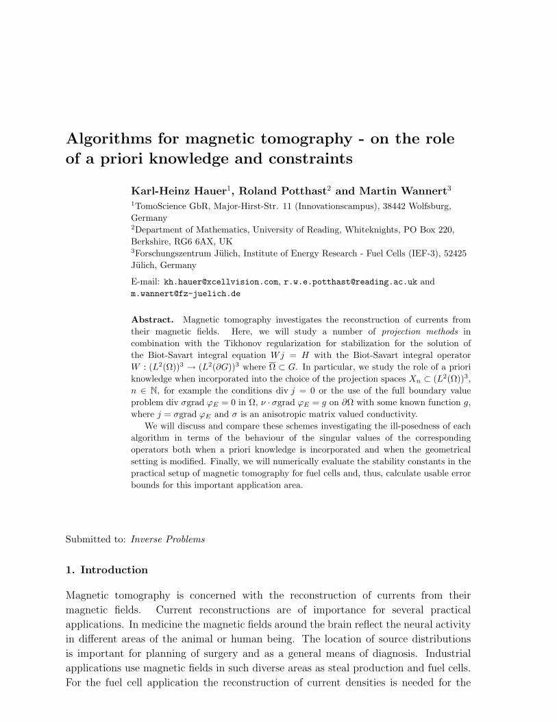
Fuel cells are chemical devices which transform chemical energy into electrical

energy. The basic principle for a hydrogen-oxygen fuel cell is shown in Figure 1. At

the anode (-) hydrogen is inserted. Air or oxygen, respectively, is fueled at the cathode

(+). They are separated by a semi-permeable membrane for protons coated with some

catalysor (for example platinum). Protons move to the cathode through the membrane.

This creates a potential which then drives electrones through an external wire and

power some motor or light. Hydrogen and oxygen react at the cathode to water and

heat. Usually fuel cells need some heating and cooling technology.

Figure 1. We show the principle of a fuel cell. Hydrogen and oxygen are fueled intodifferent layers. They react, creating a potential which drives electric currents throughthe wires.

Magnetic tomography in biomedical applications has a long history. We refer

the reader to the survey articles [4], [16] and [2] with extensive literature. Basic

mathematical results can be found in the books of Kaipio-Somersalo [8] and Kirsch [9].

To our knowledge, the study of the ill-posedness of the magnetic tomography problem

with respect to the use of a priori knowledge has not yet been carried out.

In contrast to the medical applications, the currents in fuel cells do not have internal

sources. This leads to an underlying partial differential equations without source terms

on the right-hand side. It strongly influences the uniqueness results (usually in the

medical setting the location and polarization of sources is reconstructed) and to some

extent the reconstruction techniques (in medical applications often a finite number of

parameters is determined searching for source locations).

The basic setting of magnetic tomography for fuel cells has been investigated

in a series of papers on numerical simulations with the Tikhonov regularization

for reconstruction [12], on the underlying anisotropic forward problem via the finite


integration technique [13], on the uniqueness question for current reconstructions in

single cell devices [7] and in full stacks [5] and on the full applied measurement method

including the design of a machine for such measurements [6]. In [14] the resolution of

the reconstructed current density depending on the relative error in the magnetic field

measurements is discussed. Sampling and probe methods for magnetic tomography have

been investigated in [11] and [15]. More general introductions into solution techniques

for inverse problems can be found in [3] and [1].

Next, we describe the underlying model from which parts will be incorporated into

our reconstruction algorithms later. Consider a geometrical setting as shown in Figure

2. We will model the active area of the fuel cell as a simple cube, where current is

injected into the cube at some point on the bottom and is flowing out at another point

on the back side. This means we know the total current in the cell and, in particular,

we know the inflowing and outflowing current on the boundary of the domain Ω. This

leads to the boundary condition

ν · j(y) = g, y ∈ ∂Ω (1)

with some given function g on ∂Ω. In this work we will restrict our attention to the

static situation, where the currents j do not depend on time. The behaviour of time-

independent currents, electric and magnetic fields is governed by the stationary Maxwell

equations

∇×H = j, ∇× E = 0 (2)

∇ ·D = ρ, ∇ ·B = 0 (3)

complemented by the material equations

D = εε0E, B = µµ0H (4)

and Ohm’s law

j = σE. (5)

Here, E is the electric field, D the electric flux density, H the magnetic field stength,

B the magnetic flux density, j the current density, ρ the electric charge density, σ the

conductivity distribution, ε the electric permittivity and µ the magnetic permeability of

the medium under consideration, ε0 and µ0 are the well-known natural constants for the

vacuum. For the fuel-cell application equations (5) - (6) are a macroscopic model with

some effective conductivity σ with summarizes the influence of chemical processes, fluid

dynamics of oxygen and hydrogen and the shape of the flow field into some mesoscopic

variable.

The above equations are usually transformed into an elliptic boundary value

problem, [13], for which then unique solvability is shown. Assume that Ω is simply

connected. Because of ∇×E = 0 there is an electric potential ϕE such that E = ∇ϕE,

i.e. for the current density j we have the equation j = σ∇ϕE. We use the identity


∇ · ∇ × A = 0, which is valid for any arbitrary sufficiently smooth vectorfield A, to

derive the equation

∇ · j = ∇ · ∇ ×H = 0 (6)

from the Maxwell equations (2), i.e. the current distribution is divergence free. This will

be one of the conditions included into the inversion later. Now, we obtain the equation

∇ · σ∇ϕE = 0 in Ω (7)

for the electric potential ϕE. Additionally, we have the boundary condition

ν · j = ν · σ∇ϕE = g (8)

mentioned above. We further require the additional normalization condition∫Ω

ϕEdy = 0 (9)

to establish uniqueness for this particular Neumann problem, compare [13].

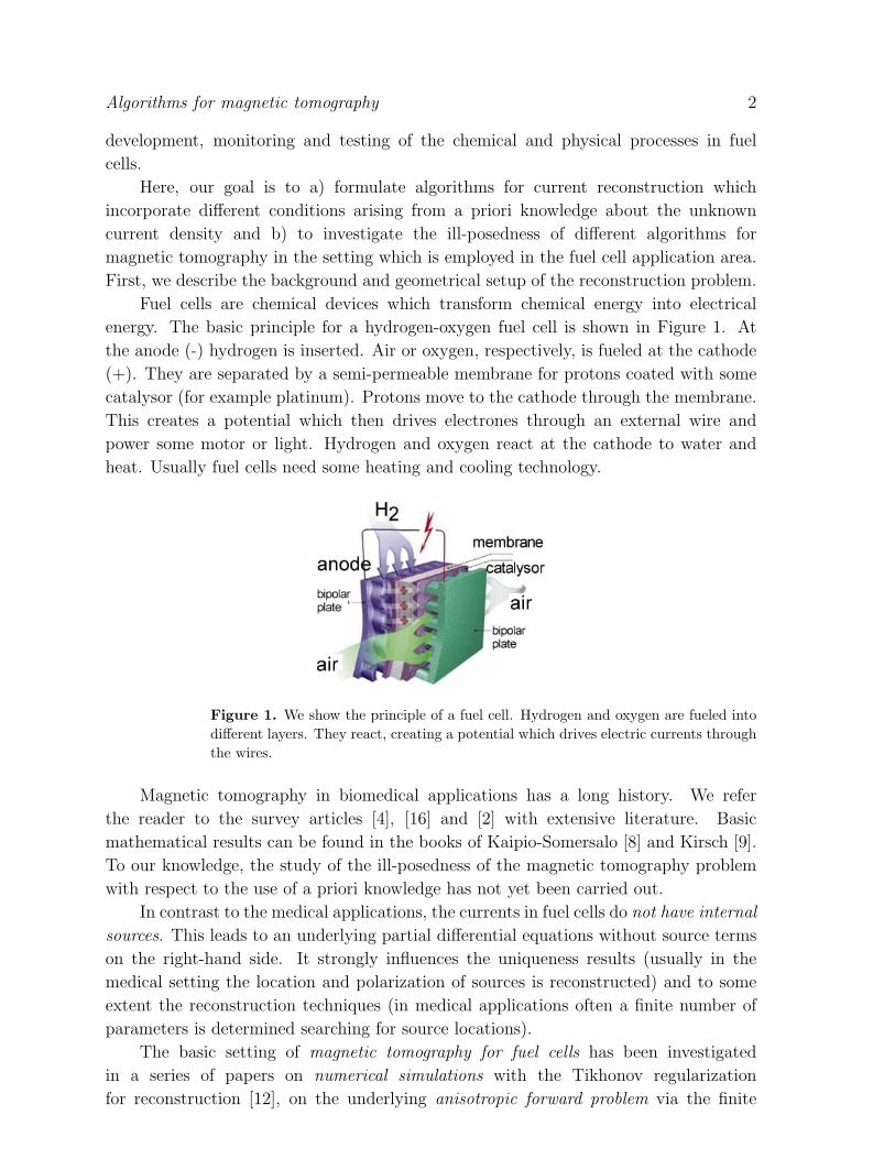
Figure 2. We show a fuel cell (left) and fuel cell stack (right) in the laboratory. Themagnetic tomograph is seen in the left image with two magnetic sensors. By courtesyof TomoScience GbR, Wolfsburg / Research Center Julich, Germany

Let us now assume that we know the current distribution j in the domain Ω ⊂ R3.

Magnetic fields H of currents j are calculated via the Biot-Savart integral operator,

defined by

(Wj)(x) :=1

4π

∫Ω

j(y)× (x− y)

|x− y|3dy, x ∈ R3 (10)

for a current density distribution j ∈ L2(Ω)3. The task of magnetic tomography in its

general form reduces to solving the equation

Wj = Hmeas on ∂G, (11)

where G is some domain with sufficiently smooth boundary such that Ω ⊂ G and

Hmeas denotes some measured magnetic field on ∂G. As discussed in [12], in principle

it is sufficient to know the normal component of H on the measurement surface ∂G.

However, we will work with the full field H, i.e. with redundant data which is used in


the practical applications (compare Figure 2) to obtain a better control of measurement

error.

The nullspace of the Biot-Savart integral operator was studied in detail in [5],

where a characterization of N(W ) and its orthogonal space N(W )⊥ has been derived.

In particular, we have

N(W ) = curl v : v ∈ H10 (Ω)3, div v = 0 (12)

with H10 (Ω) := v ∈ H1(Ω)3 : v|∂Ω = 0. Additionally, the orthogonal complement of

N(W ) with respect to the L2-scalar product on Ω is given by

N(W )⊥ = j ∈ Hdiv =0(Ω)3 : ∃q ∈ L2(Ω)3 s. th. curl j = grad q (13)

with Hdiv =0 := v ∈ L2(Ω) : div v = 0. Further, it has been shown that for a

homogeneous conductivity distribution σ the solution of (6)-(9) is in N(W )⊥ and, thus,

in this case we obtain full reconstructability.

Our key goal here is to investigate appropriate conditions on the current density

distributions j to reduce the ill-posedness of the inversion and to improve the

reconstructions achieved in [12] by plain Tikhonov regularization. In particular, we

study these three algorithms:

(A) The plain Tikhonov regularization

(B) The use of the condition (6) to supplement the equation (11).

(C) The incorporation of the full boundary value problem (7) - (9) into equation (11).

We will show how the ill-posedness of the inversion is reduced via the conditions (B)

and (C). In particular, a) we derive qualitative estimates of the singular values of the

operators under consideration and b) we provide numerical results about the quantitative

improvements which can be gained. These are compared with the improvements which

can be achieved by changing central inversion parameters like the distance of the

measurement points to the area Ω of the current density j.

We will introduce the discretized form of the Biot-Savart integral operator via a

finite integration technique in Section 2, which serves as our toolbox for the subsequent

sections. In Section 3 we discuss the methods (B) and (C). Section 4 serves to analyse

and compare the stability for the algorithms under consideration by estimates for their

singular values. Finally, in Section 5 we compare reconstruction results and we provide

a numerical evaluation of the stability constants for real settings which is typically used

for state-of-the-art devices of magnetic tomography.

2. Continuous and discrete realization of the Biot-Savart operator

The goal of this section is to summarize the finite integration technique applied to

magnetic tomography. The convergence of the technique towards the solution of

the continuous problem (1) - (5) has been analysed by Kuhn et al [13]. Since the

discretization is directly integrated into our inverse algorithms in the subsequent parts


we provide basic notation here and summarize the results. We will investigate the

situation where

Ω :=

y ∈ R3,

−a1

2< y1 <

a1

2,−a2

2< y2 <

a2

2,−a3

2< y3 <

a3

2

(14)

with some parameters a1, a2, a3 > 0. We employ a discretization with levels n1, n2, n3 in

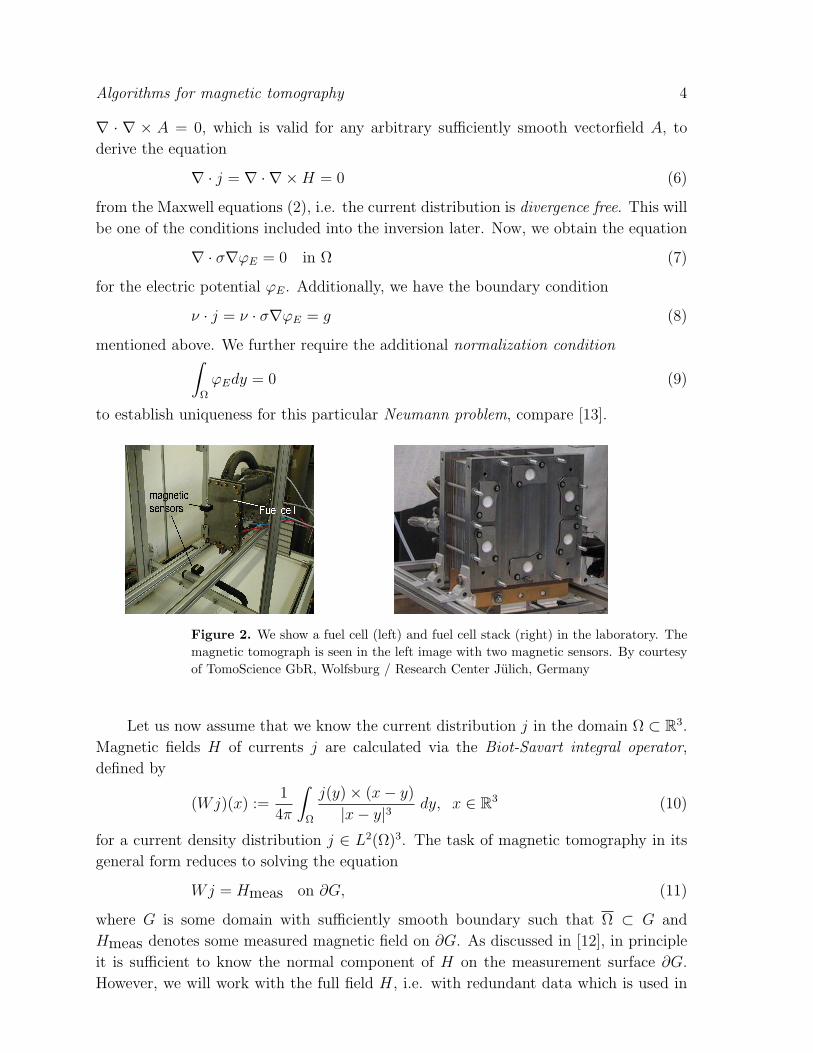
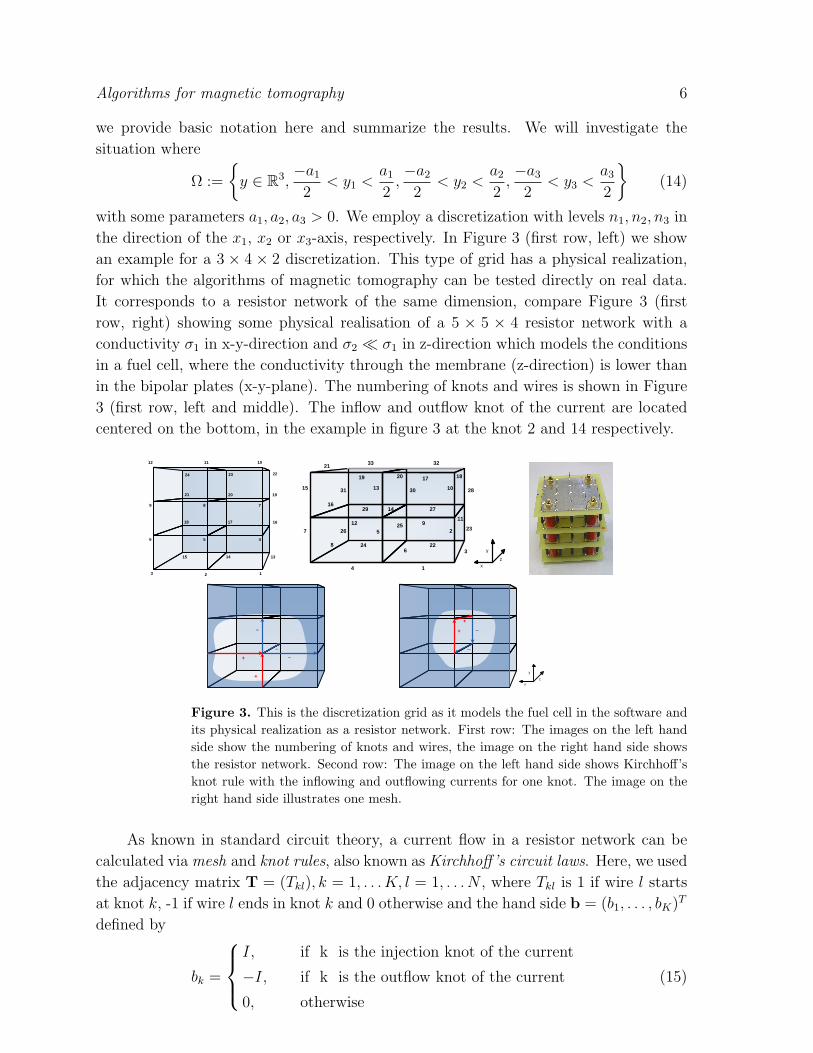
the direction of the x1, x2 or x3-axis, respectively. In Figure 3 (first row, left) we show

an example for a 3 × 4 × 2 discretization. This type of grid has a physical realization,

for which the algorithms of magnetic tomography can be tested directly on real data.

It corresponds to a resistor network of the same dimension, compare Figure 3 (first

row, right) showing some physical realisation of a 5 × 5 × 4 resistor network with a

conductivity σ1 in x-y-direction and σ2 σ1 in z-direction which models the conditions

in a fuel cell, where the conductivity through the membrane (z-direction) is lower than

in the bipolar plates (x-y-plane). The numbering of knots and wires is shown in Figure

3 (first row, left and middle). The inflow and outflow knot of the current are located

centered on the bottom, in the example in figure 3 at the knot 2 and 14 respectively.

1

14

3

456

789

101112

13

2

15

161718

23

2021

2224

19

3

2

14

5

9

7

8

10

1112

13

14

15

16

1719 1820

21

6

23

24

26

22

27

28

29

3031

3233

25

y

x

z

+ –

–

–

+

+

–

–+

y

x

z

Figure 3. This is the discretization grid as it models the fuel cell in the software andits physical realization as a resistor network. First row: The images on the left handside show the numbering of knots and wires, the image on the right hand side showsthe resistor network. Second row: The image on the left hand side shows Kirchhoff’sknot rule with the inflowing and outflowing currents for one knot. The image on theright hand side illustrates one mesh.

As known in standard circuit theory, a current flow in a resistor network can be

calculated via mesh and knot rules, also known as Kirchhoff’s circuit laws. Here, we used

the adjacency matrix T = (Tkl), k = 1, . . . K, l = 1, . . . N , where Tkl is 1 if wire l starts

at knot k, -1 if wire l ends in knot k and 0 otherwise and the hand side b = (b1, . . . , bK)T

defined by

bk =

I, if k is the injection knot of the current

−I, if k is the outflow knot of the current

0, otherwise

(15)


with the total current I. For the discrete model we assume that the resistance of wire

l is given by Rl. The current Jl flowing through wire l, the resistance Rl of wire l and

the voltage Ul between the two endpoints of wire l are connected via Ohm’s law

Ul = Rl · Jl. (16)

The knot rules are then given by

N∑l=1

TklJl = bk, k = 1, . . . , K. (17)

The construction of the mesh rules has been realized as follows. For every knot k we

take an outgoing wire in positive direction of an arbitrary axis that ends at knot k.

Starting from k we take a wire in positive direction of an axis that is different to the

one chosen before. Then the mesh is closed by choosing exactly two additional wires.

By iterating this procedure over all knots we get the linear system

N∑l=1

Sml(RlJl) = 0, m = 1, . . . ,M, (18)

where Sml is 1 if wire l is part of mesh m and the wire is passed through in positive

direction and −1 if it is passed through in negative direction respectively. Otherwise

Sml is 0.

This procedure results in 3n1n2n3 − n1n2 − n1n3 − n2n3 + 1 equations for the

3n1n2n3 − n1n2 − n1n3 − n2n3 currents, with one redundant equation due to the

solenoidality of the electric potential. Here, we drop the last equation to obtain a

uniquely solvable system.

Having calculated the currents we are able to calculate the magnetic field at a point

x ∈ R3 via the discrete Biot-Savart operator for this wire grid. This reduces to calculate

(WJ)(x) = − 1

4π

∑wires l

∫l

Jl × (x− p)

|x− p|3ds(p), (19)

with Jl := (Jl, 0, 0)T , if wire l is parallel to the x-axis, Jl := (0, Jl, 0)T , if wire l is parallel

to the y-axis or Jl := (0, 0, Jl)T , if wire l is parallel to the z-axis. Here, we have used an

exact integration of the magnetic field for a straight wire as explicitly given by equation

(4.9) in [5].

The convergence theorem for the finite integration technique towards the solution of

the continuous problem (1) - (5) has been shown in [13], where the discretized problem

is extended into the three-dimensional space via interpolation.

Theorem 2.1 Let σ be a coercitive matrix. Then the equation system arising from

mesh and knot rules has a unique solution for each discretization (n1, n2, n3). For

nj →∞, j = 1, 2, 3 it converges towards the true solution of the boundary problem.


3. Algorithms for magnetic tomography

The Biot-Savart operator W is a linear and bounded operator from (L2(Ω))3 to

(L2(∂G))3. Since it has an analytic kernel it is well-known from standard functional

analysis that it is a compact operator ([10], Thm. 2.21) with exponentially decaying

singular values. It can not be continuously invertible ([10], Thm. 2.20). This leads to

highly unstable reconstructions where small pertubations in the right hand side of (11)

cause strong pertubations in the solution and is one of the main limitations of magnetic

tomography.

Discretizing the Biot-Savart operator as described in the previous section we get the

3n×N matrix W, where n is the number of measurement points on the measurement

surface ∂G and N is the number of wires in the cube. We usually assume 3n N , i.e.

we work with overdetermined systems. Then, the discretized form of (11) is given by

WJ = Hmeas. (20)

It has been shown in [5] that W is injective. However, this finite dimensional system

is strongly ill-conditioned where the condition number increases exponentially when

the approximation level is increased. The basic principle of regularization methods

for injective operators is to approximate the unbounded operator W−1 by a bounded

operator Rα with regularization parameter α > 0 which shows pointwise convergence

RαH → j := W−1f, α → 0, for H = Wj. If W is not injective, we cannot expect

RαH → j, but we usually we have RαH → Pj, α → 0, with some projection operator

P . For continuous Tikhonov regularization the projection P is the orthogonal projection

onto N(W )⊥. For the discrete case, classical Tikhonov regularization [17] employs

Rα := (αI + W∗W)−1W∗ (21)

with regularization parameter α > 0, where W∗ denotes the complex conjugate

transpose matrix of W. For the choice of the regularization parameter we refer to

standard results in [3]. Plain Tikhonov regularization has been applied to magnetic

tomography problem in [12] which proves in principle the feasibility of current

reconstructions for the inverse problem (11), but also demonstrates its severe ill-

posedness. We denote the classical algorithm (21) by A. In the following subsections

we combine projection algorithms where further knowledge is incorporated into the

inversion procedure with Tikhonov type regularization schemes.

3.1. Divergence free Tikhonov regularization

We recall that the current distribution j is divergence free and it is natural to incorporate

condition (6) into the inversion. We expect this condition to decrease the solution

space to provide a more accurate solution and will provide qualitative estimates and

quantitative results in the next sections.

For the discrete realization of the inversion we use the condition introduced in

equation (17) for choosing the finite subset Xn of the solution space (L2(Ω))3. This


condition corresponds to Kirchhoff’s knot rule, so we set up the matrix T as described

in section 2. Since the discrete solution J solves

TJ = b, (22)

with a particular solution j0 the general solution of this equation is given by

jgen = j0 + Nz, (23)

with a basis N of the nullspace of T and arbitrary z. Inserting this representation into

equation (20) we derive

(WN)z = Hmeas −Wj0 (24)

which can be solved via Tikhonov regularization by setting

Rα := (αI + (WN)∗(WN))−1(WN)∗, α > 0. (25)

Now a solution J of (20) can be obtained by setting

J := j0 + NRα(Hmeas −Wj0). (26)

A concise formulation of this algorithm is given by the following pseudo code.

Algorithm B. Divergence free Tikhonov regularization

function DivergenceFreeTikhonov(α,b,Hmeas)

calculate W via finite integration

calculate T from (17)

calculate particular solution j0 of TJ = b

caluclate orthonormal basis N of N(T)

Rα ← (αI + (WN)∗(WN))−1(WN)∗

J← j0 + NRα(Hmeas −Wj0)

return J

end function

Numerical results for the algorithm are shown in section 5. We estimate the singular

values of WN in section 4.

3.2. A projection method with special basis functions

In this section we will take into account the information that our currents solve the

boundary value problem (6) - (9). This leads to a projection method with a special

basis j(k) : k = 1, . . . N. Here, we construct this basis such that its z-components

approximately build a Haar basis, i.e. they are approximately a multiple of 1 in some

section and close to zero in all others.

As background we remind the reader that for the fuel cell application the

conductivity in x − y layers are usually large and uniform due to metallic end plates

and carbon layers between the different single fuel-cells. Thus, we use a uniform high

conductivity σ0 in all wires in x− y direction. We have varying conductivity only in the


wires in z-direction, which we label from k = 1 to k = N . Now, we choose numbers σl,

l = 0, 1, 2 with

σ2 σ1 σ0. (27)

Then, the idea is to use the ansatz

j =N∑

k=1

ξkjk, (28)

where jk is a current distribution with a conductivity which is set to σ1 in wire

k in z-direction and to σ2 in all other wires in z-direction. We use the notation

XN := spanjk : k = 1, ..., N. The current distributions jk, k = 1, . . . , N are solutions

to the forward problem, i.e. they are calculated via knot and mesh rules as described in

section 2. The magnetic field of an element j ∈ XN at a point x ∈ R3 can be calculated

via

(Wj)(x) =N∑

k=1

ξk(Wjk)(x). (29)

Defining Hk := Wjk by evaluating the Biot-Savart operator, we set up the matrix

Hs := (H1, . . . , HN). Then, we solve the ill-posed linear system

Hsξ = Hmeas (30)

for the coefficients ξ := (ξ1, . . . , ξN)T , where we employ Tikhonov regularization for

regularization of this system. The solution J of the original problem is obtained by

calculating

J :=N∑

k=1

ξkjk. (31)

In view of Section 4, Theorem 4.4, we note that in general the jk are not an

orthonormal basis of the discrete space XN . However, we can orthonormalize jk to

obtain a basis jk,o : k = 1, ..., N of XN and define Hs,o := (Wj1,o, ..,WjN,o). Then

all estimates below apply. However, for simplicity we have usually directly applied the

special basis method via Hs with satisfying results. We conclude this section with the

pseudo code presentation of the special basis projection method.


Algorithm C. Special basis projection

function SpecialBasisProjection(α,Hmeas)

calculate W via finite integration

for k = 1, . . . , N do

calculate current distribution jk as described in (27)

Hk ←Wjk

end for

Hs := (H1, · · · , HN)

Rα ← (αI + H∗sHs)

−1H∗s

ξ ← RαHmeasJ←

∑Nk=1 ξkjk

return J

end function

Numerical results for the algorithm are shown in section 5 and we estimate the

singular values of the orthonormalized version Hs,o of Hs in section 4.

4. Algorithmic stability analysis in dependence on a priori knowledge

In this section we study the stability of the above algorithms via their singular values

and derive estimates for the singular values of the methods.

Usually, for estimating the ill-posedness of inverse problems the size of the singular

values is taken as central measure. For discrete inverse problems the condition number

is the key quantity. Here, we are mostly interested in the singular values as becomes

clear from the following reasons. Consider an equation

Ax = b (32)

which we solve with some data error e(δ), i.e. we calculate x(δ) by

A(x(δ)) = b + e(δ). (33)

In general one estimates the error by

||x− x(δ)|| ≤ ||A−1|| · ||e(δ)|| (34)

and calculates the relative error

||x− x(δ)||||x||

≤ ||A−1|| · ||A|| · ||e(δ)||||b||

. (35)

Thus, the condition number provides an upper bound for the relative numerical error.

Now, we consider two matrices A1, A2 with A1x = b and A2x = b, where the singular

values of A2 are larger than the singular values of A1, thus the norm ||A−12 || is smaller

than the norm ||A−11 ||. Still, the condition of A2 might be larger than the condition of

A1, which is partly the case for our setting of magnetic tomography. If we solve the


same problem with given data we need to consider the case where we keep e(δ) fixed.

Then, we solve the systems

A1x(δ)1 = b + e(δ), A2x

(δ)2 = b + e(δ), (36)

Estimating the reconstruction error ||x− x(δ)|| as in (34) we have

||A−12 || · ||e(δ)|| ≤ ||A−1

1 || · ||e(δ)||, (37)

i.e. we have a better estimate for the data error from the second system with A2 than

for the system with A1. Here, the true solution x is fixed. In this case from (37) we get

a better estimate for the relative error via the second system

||x− x(δ)2 ||

||x||≤ ||A

−12 || · ||b||||x||

||e(δ)||||b||

, (38)

compared to the estimate for the first system

||x− x(δ)1 ||

||x||≤ ||A

−11 || · ||b||||x||

||e(δ)||||b||

. (39)

If the error is a multiple of the eigenvector with smallest singular value of A1, then

the estimate (39) will be sharp and the improvement in the error is fully given by the

improvement in the estimate (37) of the norm of the inverse via the singular values.

The estimate (38) fully carries over to (24): one calculates

(WN)z = Hmeas −Wj0 ⇒ (WN)(z − z(δ)) = e(δ)

⇒ x− x(δ) = N(z − z(δ)) = N(WN)−1e(δ) (40)

Since N has orthonormal columns we obtain (38) also for a setting of the form (24).

For general estimates of the singular values we will use the Courant minimum

maximum principle as a key tool. First, we order the eigenvalues of a self-adjoint matrix

operator A : Cn → Cn according to their size and multiplicity λ1 ≥ λ2 ≥ . . . ≥ λn. Then,

the Courant minimum maximum principle states that

λn+1−k = mindim U=k

maxx∈U

(Ax, x)

(x, x), k = 1, . . . , n. (41)

We use this to prove some useful properties. Roughly speaking, the aim of this section is

to show that incorporating some a priori knowledge leads to larger singular values of the

corresponding Tikhonov matrix. We set up a general framework in terms of subspaces

and apply this to our setting of magnetic tomography.

Definition 4.1 (A priori knowledge via subspace setting) We denote X =

Cn and Y = Cm and we consider an operator W : X → Y . For a subspace V ⊂ X = Cn

we define WV : V → Y by WV = W |V and W ∗V to be its adjoint operator Y → V

determined by

(Wx, y)Y = (x, W ∗V y)V , x ∈ V, y ∈ Y. (42)

It is well known that

N(W ∗V ) = W (V )⊥. (43)


Clearly, the operator AV := W ∗V W is a self adjoint operator on V , since for x, z ∈ V we

have

(z, W ∗V Wx)V = (WV z, Wx)Y = (W ∗

V WV z, x)V . (44)

First, we collect some properties of the adjoint operators arising from the subspaces

V ⊂ V ⊂ X.

Lemma 4.2 Let V ⊂ V ⊂ X be subspaces and consider the adjoint operators W ∗V of

WV : V → Y and W ∗V

of WV : V → Y arising from the restriction of W to V or V ,

respectively. Further, let P : V → V denote the orthogonal projection operator from V

onto V ⊂ V . Then we obtain

W ∗V

= PW ∗V . (45)

Proof. We denote Q := I − P and decompose x = Qx + Px for x ∈ V . For

x ∈ V , y ∈ Y we obtain Qx = 0 and in this case we calculate

(x, PW ∗V y)

P=I−Q= (x, W ∗

V y −QW ∗V y)

Qx=0= (Px,W ∗

V y −QW ∗V y) (46)

P (V )⊥Q(V )= (x, W ∗

V y) = (WV x, y)x∈V⊂V

= (WV x, y) = (x, W ∗Vy).

This yields (x, (PW ∗V −W ∗

V)y) = 0 for all x ∈ V , from which (45) follows.

We now prove a monotonicity property for singular values which directly applies to

the setting of magnetic tomography.

Theorem 4.3 Let V, V ⊂ Cn be subspaces of Cn with V ⊂ V and denote the singular

values of WV or WV , respectively, by µj or µj, j = 1, 2, 3, . . . . We denote the dimensions

of V, V by n, n and note that n ≤ n by V ⊂ V . Then we obtain the estimates

µn+1−j ≤ µn+1−j, j = 1, 2, 3, . . . , n. (47)

Moreover, in this estimate we will obtain equality for k ∈ N if and only if the eigenspace

Ek of W ∗V WV with eigenvalue λn+1−k is a subset of V .

Proof. We employ the Courant minimum maximum principle applied to the

eigenvalues λk of W ∗V WV and the eigenvalues λk of W ∗

VWV to derive

λn+1−k = minU⊂V,dim U=k

(maxx∈U

(W ∗V WV x, x)

(x, x)

)= min

U⊂V,dim U=k

(maxx∈U

(WV x, WV x)

(x, x)

)≤ min

U⊂V ,dim U=k

(maxx∈U

(WV x, WV x)

(x, x)

)= min

U⊂V ,dim U=k

(maxx∈U

(WV x, WV x)

(x, x)

)= min

U⊂V ,dim U=k

(maxx∈U

(W ∗VWV x, x)

(x, x)

)= λn+1−k (48)


for k = 1, 2, . . . , n. In this estimate we will obtain equality for k ∈ N if and only if all

subspaces U with a dimension dim(U) = k of the eigenspace Ek corresponding to the

eigenvalue λn+1−k (which are spaces U where the Courant minimax principle attains its

minimum) are subsets of V . This is equivalent to the eigenspace Ek being a subset of

V .

We apply the result to our algorithms for magnetic tomography as follows.

Theorem 4.4 Consider the three solution methods (A), (B) and (C) from Section 1:

(A) the plain Biot-Savart equation biven by (20),

(B) the divergence free Biot-Savart equation as in (24) and

(C) the special basis Biot-Savart equation (30).

Here, for (30) we assume that the basis currents j1, . . . , jN build an orthonormal set in

the space of all currents. Then for the singular values µ(A)k , µ

(B)k and µ

(C)k of the matrices

W(A) := W, W(B) := WN and W(C) := Hs,o we obtain the estimates

µ(A)nA+1−k ≤ µ

(B)nB+1−k ≤ µ

(C)nC+1−k (49)

for k = 1, 2, . . . , nC.

Proof. The generic case is provided by a matrix W and a matrix N with

orthonormal columns. In this case we can interpret the mapping z 7→ Nz as a restriction

of the mapping W to the image space V := v1, . . . , vm where vj are the columns of

N. Let U ⊂ Cm be a subset. Then

minU⊂Cm,dim U=k

(maxz∈U

(WNz,WNz)

)= min

U⊂V,dim U=k

(maxx∈U

(WNx,WNx)

)(50)

with V := N(Cm), because N maps the set of subspaces of Cm bijectively onto the set

of subspaces of V . From this follows that WN and W|V have the same singular values.

The mapping z 7→ Nz is norm preserving. Now, an application of Theorem 4.3

proves an estimate of the form (49).

For the comparision of (B) and (C) we remark that the matrix arising from Wjk can

be written as WJ with the orthonormal matrix J = (j1, . . . , jN). We remark that since

the jk are calculated from equations (17) and (18) are divergence free. The estimate is

then obtained as above from Theorem 4.3.

We have shown that the use of a priori knowledge via knot equations and special

basis functions which incorporate the background knowledge leads to better estimates

for inversion than the general Biot-Savart equation. Moreover, the estimate of the

singular values provides a strong spectral analysis of the situation, which can be used

in more detail. Here, we next will provide a numerical study of the situation which

confirms the above estimates and also demonstrates the actual size of the constants for

some important sample settings frequently used for the practical application of magnetic

tomography.


5. Evaluation of stability constants for a realistic setup

We use a 7 × 7 × 2-grid to simulate a single-cell device as presented in figure 4. 296

measurement points are placed equidistantly in distance of 60 mm around the wire grid.

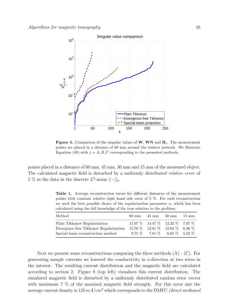
In the following we will present a numerical spectral analysis done for this important

sample setting. Figure 5 shows the singular values of the matrices W, WN and Hs

that were presented in section 3 for this setting. In this example the magnitude of the

smallest singular values differ by a factor between 10 and 100 as well between algorithms

(A) and (B) as between algorithms (B) and (C).

200 mm

160 mm

140 mm

280 m

m

240 m

m

180 m

m

Active cell area (MEA)

Flowfield (graphite)

Endplate (non-magnetic steel)

Figure 4. Real cell components (endplate, flowfield and membrane electrode assembly(MEA)), dimension of the cell components.

Figure 6 shows a comparison of the reciprocal of the singular values of each matrix

and the singular values of the corresponding Tikhonov matrix.

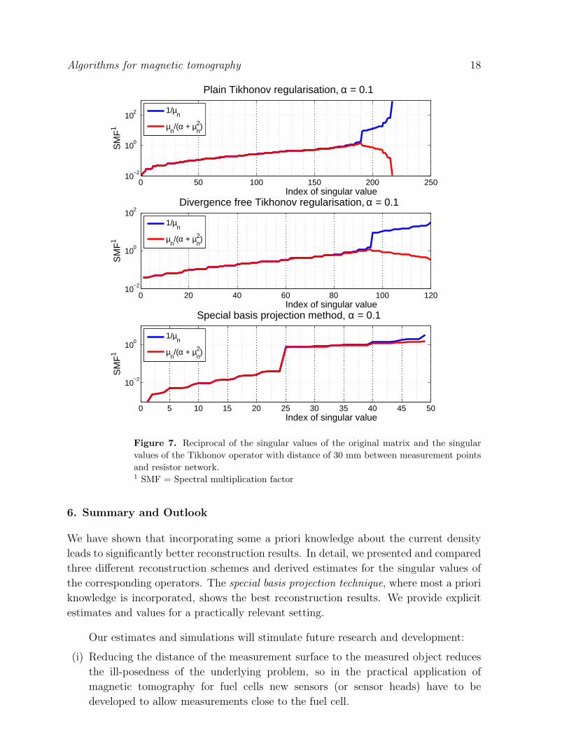
We expect, that the ill-posedness of the problem decreases, when the observation

distance is reduced. We present a short overview in which manner this happens by

showing reconstruction errors for different observation distances and a comparison of the

singular values, where the distance between the measurement surface and the measured

object is reduced to 30 mm. The size of the singular values differs by a factor of 100

uniformly over all three methods by halfening the distance between the measurement

surface and the measured object. The behavior of the reciprocal of the singular values

compared to the singular values of the Tikhonov matrix is illustrated in figure 7. Table 1

shows reconstruction errors for the sample setting mentioned above for the measurement


1 50 100 150 200 250

10−4

10−2

100

102

104

Singular value comparison

k

µ(j) n j+1−

k

Plain TikhonovDivergence free TikhonovSpecial basis projection

Figure 5. Comparison of the singular values of W, WN and Hs. The measurementpoints are placed in a distance of 60 mm around the resistor network. We illustrateEquation (49) with j = A,B,C corresponding to the presented methods.

points placed in a distance of 60 mm, 45 mm, 30 mm and 15 mm of the measured object.

The calculated magnetic field is disturbed by a uniformly distributed relative error of

5 % in the data in the discrete L2-norm || · ||2.

Table 1. Average reconstruction errors for different distances of the measurementpoints with constant relative right hand side error of 5 %. For each reconstructionwe used the best possible choice of the regularization parameter α, which has beencalculated using the full knowledge of the true solution to the problem.

Method 60 mm 45 mm 30 mm 15 mm

Plain Tikhonov Regularization 17.07 % 13.47 % 12.23 % 7.07 %Divergence free Tikhonov Regularization 15.76 % 12.81 % 12.04 % 6.36 %Special basis reconstruction method 9.75 % 7.81 % 6.65 % 5.53 %

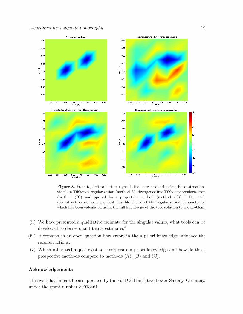
Next we present some reconstructions comparing the three methods (A) - (C). For

generating sample currents we lowered the conductivity in z-direction at two wires in

the interior. The resulting current distribution and the magnetic field are calculated

according to section 2. Figure 8 (top left) visualizes this current distribution. The

simulated magnetic field is disturbed by a uniformly distributed random error vector

with maximum 7 % of the maximal magnetic field strength. For this error size the

average current density is 125 mA/cm2 which corresponds to the DMFC (direct methanol


0 50 100 150 200 250

10−4

10−2

100

102

104

106

Plain Tikhonov regularisation, α = 0.1

Index of singular value

SM

F1

0 20 40 60 80 100 12010

−4

10−2

100

102

104

Divergence free Tikhonov regularisation, α = 0.1


SM

F1

0 5 10 15 20 25 30 35 40 45 50

10−2

100

102

Special basis projection method, α = 0.1


SM

F1

1/µn

µn/(α + µ

n2)

1/µn

µn/(α + µ

n2)

1/µn

µn/(α + µ

n2)

Figure 6. Reciprocal of the singular values of the original matrix and the singularvalues of the Tikhonov operator with distance of 60 mm between measurement pointsand resistor network1 SMF = Spectral multiplication factor

fuel cell) application, but the range in figure 8 is cut at 40mA/cm2 to make artefacts

visible.

One can see clearly the improvements resulting from incorporating a priori

knowledge as described and analyzed in sections 3 and 5. The plain Tikhonov

regularization (method (A)) identifies the spots with lowered current density correctly,

but generates strong artefact in the neighborhood of the real spots. The divergence

free Tikhonov regularization (method (B)) also identifies regions with lowered current

density, but the two distincly separated wires appear as one area with lower current

density. There are also some artefacts surrounding the identified spots. As expected

from the results of section 5 the special basis projection method (method (C)) provides

the best reconstruction results. One can see two clearly separated spots and a reduction

of the artefacts.


0 50 100 150 200 25010

−2

100

102

Plain Tikhonov regularisation, α = 0.1

SM

F1


0 20 40 60 80 100 12010

−2

100

102

Divergence free Tikhonov regularisation, α = 0.1

SM

F1


0 5 10 15 20 25 30 35 40 45 50

10−2

100

Special basis projection method, α = 0.1


SM

F1

1/µn

µn/(α + µ

n2)

1/µn

µn/(α + µ

n2)

1/µn

µn/(α + µ

n2)

Figure 7. Reciprocal of the singular values of the original matrix and the singularvalues of the Tikhonov operator with distance of 30 mm between measurement pointsand resistor network.1 SMF = Spectral multiplication factor

6. Summary and Outlook

We have shown that incorporating some a priori knowledge about the current density

leads to significantly better reconstruction results. In detail, we presented and compared

three different reconstruction schemes and derived estimates for the singular values of

the corresponding operators. The special basis projection technique, where most a priori

knowledge is incorporated, shows the best reconstruction results. We provide explicit

estimates and values for a practically relevant setting.

Our estimates and simulations will stimulate future research and development:

(i) Reducing the distance of the measurement surface to the measured object reduces

the ill-posedness of the underlying problem, so in the practical application of

magnetic tomography for fuel cells new sensors (or sensor heads) have to be

developed to allow measurements close to the fuel cell.


Figure 8. From top left to bottom right: Initial current distribution, Reconstructionsvia plain Tikhonov regularization (method A), divergence free Tikhonov regularization(method (B)) and special basis projection method (method (C)). For eachreconstruction we used the best possible choice of the regularization parameter α,which has been calculated using the full knowledge of the true solution to the problem.

(ii) We have presented a qualitative estimate for the singular values, what tools can be

developed to derive quantitative estimates?

(iii) It remains as an open question how errors in the a priori knowledge influence the

reconstructions.

(iv) Which other techniques exist to incorporate a priori knowledge and how do these

prospective methods compare to methods (A), (B) and (C).

Acknowledgements

This work has in part been supported by the Fuel Cell Initiative Lower-Saxony, Germany,

under the grant number 80013461.


References

[1] Colton D and Kress R 1998 Inverse Acoustic and Electromagnetic Scattering Theory (AppliedMathematical Sciences vol 93), 2nd edn (Berlin: Springer)

[2] Del Gratta C, Pizzella V, Tecchio F and Romani G L 2001 Magnetoencephalography a noninvasivebrain imaging method with 1 ms time resolution Rep. Prog. Phys. 64 1759–1814

[3] Engl H W, Hanke M and Neubauer A 1996 Regularization of inverse problems (Dordrecht: Kluwer)[4] Hamalainen M, Hari R, Ilmoniemi R J, Knuutila J and Lounasmaa O V 1993 Magnetoencephalog-

raphy - theory, instrumentation, and applications to noninvasive studies of the working humanbrain Rev. Mod. Phys. 65 413–97

[5] Hauer K-H, Kuhn L and Potthast, R 2005 On uniqueness and non-uniqueness for currentreconstruction from magnetic fields Inverse Problems 20 1–13

[6] Hauer K-H, Potthast R, Stolten D and Wuster T 2005 Magnetotomography - a new method foranalysing fuel cell performance and quality Journal of Power Sources 143 67–74

[7] Potthast R and Wannert M Uniqueness of Current Reconstructions for Magnetic Tomography inMulti-Layer Devices, submitted for publication

[8] Kaipio J, Somersalo E 2005 Statistical and Computational Inverse Problems Applied MathematicalSciences vol 160 (Berlin: Springer)

[9] Kirsch A 1996 An introduction to the mathematical theory of inverse problems (AppliedMathematical Science vol. 120), Berlin: Springer

[10] Kress R 1999 Linear Integral Equations (Applied Mathematical Sciences vol 82), 2nd ed (Berlin:Springer)

[11] Kuhn L 2005 Magnetic tomography - on the nullspace of the Biot-Savart operator and point sourcesfor field and domain reconstruction PhD Thesis University of Gottingen

[12] Kuhn L, Kreß R and Potthast R 2002 The reconstruction of a current distribution from its magneticfields Inverse Problems 18 1127–46

[13] Kuhn L and Potthast R 2003 On the convergence of the finite integration technique for theanisotropic boundary value problem of magnetic tomography Math. Meth. Appl. Sciences 26739–57.

[14] Lustfeld H, Reissel M, Schmidt U and Steffen B Reconstruction of electric currents in a fuel cellby magnetic field measurements J. Fuel Cell Sci. Technol., accepted for publication

[15] Potthast R 2006 A survey on sampling and probe methods for inverse problems. Topical ReviewInverse Problems 22 R1-47

[16] Sarvas J 1987 Basic mathematical and electromagnetic concepts of the biomagnetic inverse problemPhys. Med. Biol. 32 11–22

[17] Tikhonov A N 1962 On the solution of incorrectly formulated problems and the regularizationmethod Soviet Math. Doklady 4 1035–38, english translation

Date post:	09-Jan-2022
Category:	Documents
Upload:	others
View:	0 times
Download:	0 times

Algorithms for magnetic tomography - on the role of a ...

Documents