Computer Science Journal of Moldova, vol.4, no.3(12), 1996

Algorithms in Singular

Hans Schonemann

Abstract

Some algorithms for singularity theory and algebraicgeometry

The use of Grobner basis computations for treating systemsof polynomial equations has become an important tool in manyareas. This paper introduces of the concept of standard bases(a generalization of Grobner bases) and the application to someproblems from algebraic geometry. The examples are presentedas Singular commands. A general introduction to Grobnerbases can be found in the textbook [CLO], an introduction tosyzygies in [E] and [St1].

Singular is a computer algebra system for computing infor-mation about singularities, for use in algebraic geometry. The ba-sic algorithms in Singular are several variants of a general stan-dard basis algorithm for general monomial orderings(see [GG]).This includes wellorderings (Buchberger algorithm ([B1],[B2]) andtangent cone orderings (Mora algorithm ([M1],[MPT])) as specialcases: It is able to work with non-homogeneous and homogeneousinput and also to compute in the localization of the polynomialring in 0. Recent versions include algorithms to factorize polyno-mials and a factorizing Grobner basis algorithm. For a completedescription of Singular see [Si].

1 Basic definitions

1.1 Monomial orderings

The basis ingredience for all standard basis algorithms is the orderingof the monomials (and the concept of the leading term: the term withthe highest monomial).

c©1996 by Hans Schonemann

315

Hans Schonemann

A monomial ordering (term ordering) on K[x1, . . . , xn] is a totalordering < on the set of monomials (power products) xα|α ∈ Nnwhich is compatible with the natural semigroup structure, i.e. xα < xβ

implies xγxα < xγxβ for any γ ∈ Nn.The ordering < is called a wellordering iff 1 is the smallest mono-

mial. Most of the algorithms work for general orderings.Robbiano (cf.[R]) proved that any semigroup ordering can be de-

fined by a matrix A ∈ GL(n,R) as follows (matrix ordering):Let a1, . . . , ak be the rows of A, then xα < xβ if and only if there

is an i with ajα = ajβ for j < i and aiα < aiβ. Thus, xα < xβ ifand only if Aα is smaller than Aβ with respect to the lexicographicalordering of vectors in Rn.

We call an ordering a degree ordering if it is given by a matrixwith coefficients of the first row either all positive or all negative.

Let K be a field; for g ∈ K[x], g 6= 0, let L(g) be the leadingmonomial with respect to the ordering <1 and c(g) the coefficient ofL(g) in g, that is g = c(g)L(g)+ smaller terms with respect to <.

< is an elimination ordering for xr+1, . . . , xn iff L(g) ∈K[x1, . . . , xr] implies g ∈ K[x1, . . . , xr]).

1.2 Examples for monomial orderings

Important orderings for applications are:

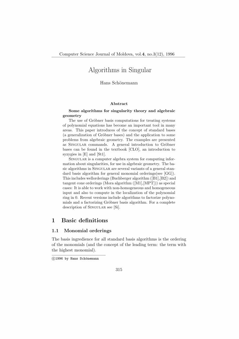
• The lexicographical ordering lp, given by the matrix:

11 0

. . .0 1

1we write the terms of a polynomial in decreasing order

316

Algorithms in Singular

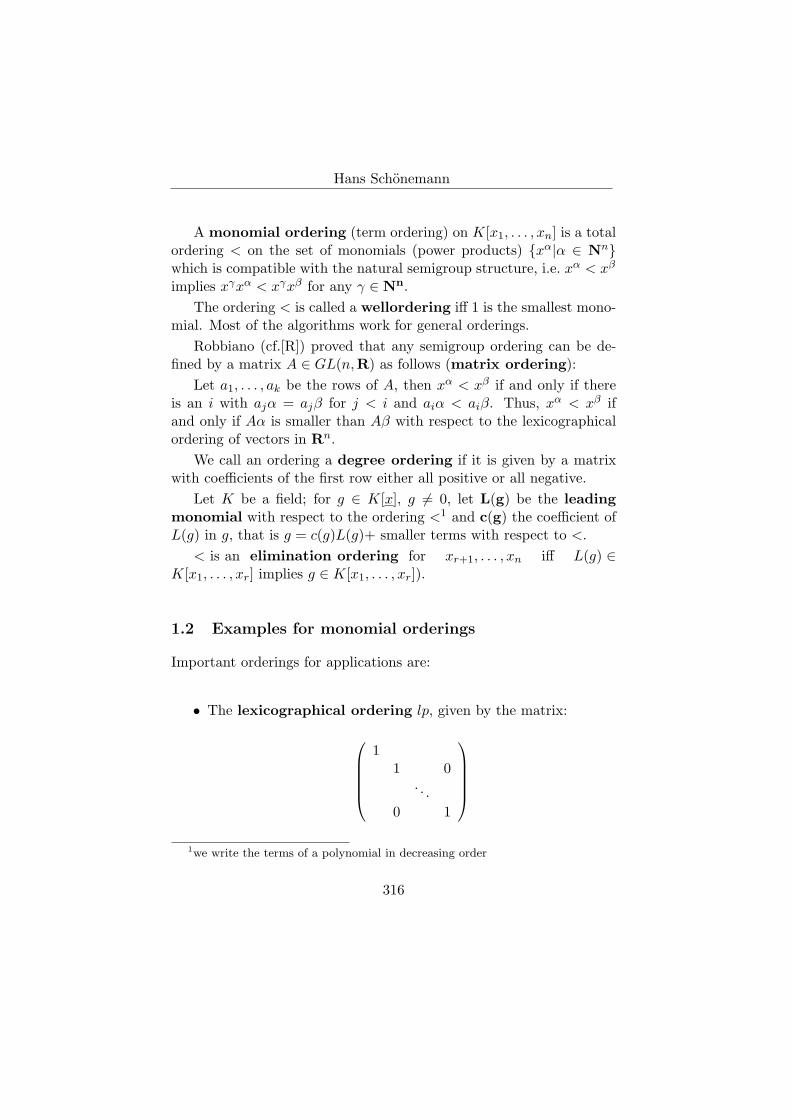
resp. ls:

−1−1 0

. . .0 −1

Remark 1.1 The positive lexicraphic ordering lp on K[x1, . . . ,xn] is an elimination ordering for x1, . . . , xi ∀1 ≤ i ≤ n

The definition of rings with these orderings in Singular:(Each line starting with // is a comment in Singular.)

ring R1=0,(x(1..5)),lp;ring R2=0,(x(1..5)),ls;

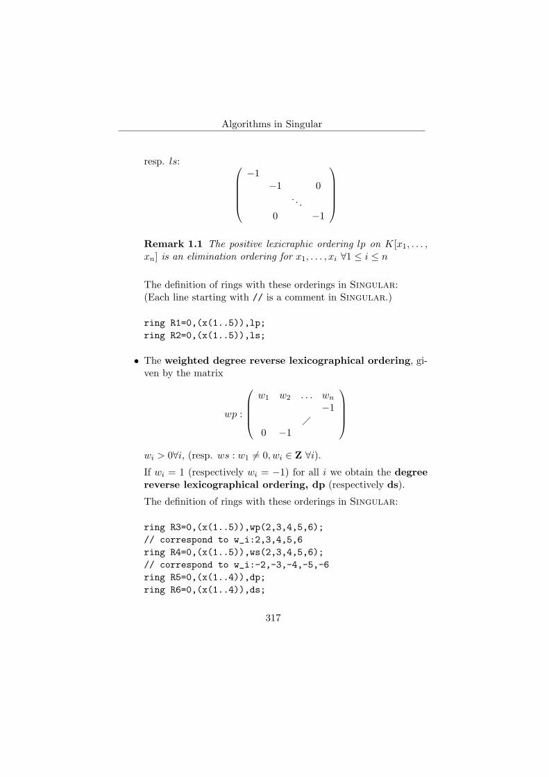
• The weighted degree reverse lexicographical ordering, gi-ven by the matrix

wp :

w1 w2 . . . wn

−1

0 −1

wi > 0∀i, (resp. ws : w1 6= 0, wi ∈ Z ∀i).If wi = 1 (respectively wi = −1) for all i we obtain the degreereverse lexicographical ordering, dp (respectively ds).

The definition of rings with these orderings in Singular:

ring R3=0,(x(1..5)),wp(2,3,4,5,6);// correspond to w_i:2,3,4,5,6ring R4=0,(x(1..5)),ws(2,3,4,5,6);// correspond to w_i:-2,-3,-4,-5,-6ring R5=0,(x(1..4)),dp;ring R6=0,(x(1..4)),ds;

317

Hans Schonemann

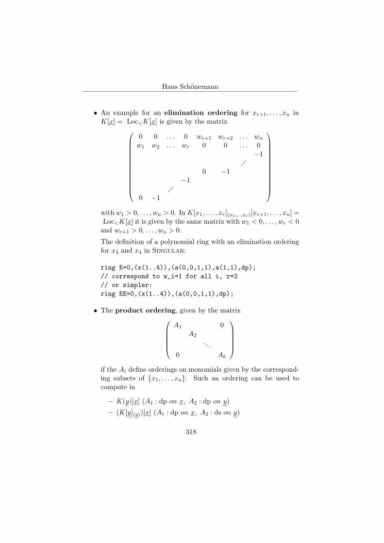
• An example for an elimination ordering for xr+1, . . . , xn inK[x] = Loc<K[x] is given by the matrix

0 0 . . . 0 wr+1 wr+2 . . . wn

w1 w2 . . . wr 0 0 . . . 0−1

0 −1

−1

0 −1

with w1 > 0, . . . , wn > 0. In K[x1, . . . , xr](x1,...,xr)[xr+1, . . . , xn] =Loc<K[x] it is given by the same matrix with w1 < 0, . . . , wr < 0

and wr+1 > 0, . . . , wn > 0.

The definition of a polynomial ring with an elimination orderingfor x3 and x4 in Singular:

ring E=0,(x(1..4)),(a(0,0,1,1),a(1,1),dp);// correspond to w_i=1 for all i, r=2// or simpler:ring EE=0,(x(1..4)),(a(0,0,1,1),dp);

• The product ordering, given by the matrix

A1 0A2

. . .0 Ak

if the Ai define orderings on monomials given by the correspond-ing subsets of x1, . . . , xn. Such an ordering can be used tocompute in

– K(y)[x] (A1 : dp on x, A2 : dp on y)

– (K[y](y))[x] (A1 : dp on x, A2 : ds on y)

318

Algorithms in Singular

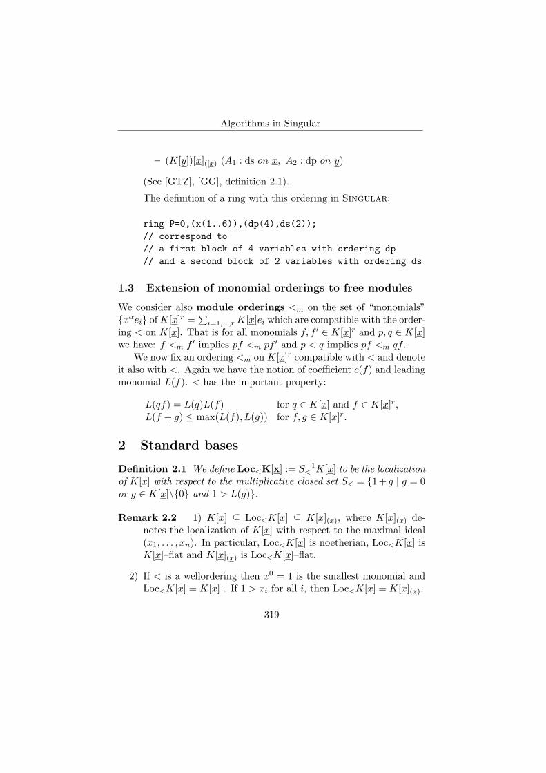
– (K[y])[x]([x) (A1 : ds on x, A2 : dp on y)

(See [GTZ], [GG], definition 2.1).

The definition of a ring with this ordering in Singular:

ring P=0,(x(1..6)),(dp(4),ds(2));// correspond to// a first block of 4 variables with ordering dp// and a second block of 2 variables with ordering ds

1.3 Extension of monomial orderings to free modules

We consider also module orderings <m on the set of “monomials”xαei of K[x]r =

∑i=1,...,r K[x]ei which are compatible with the order-

ing < on K[x]. That is for all monomials f, f ′ ∈ K[x]r and p, q ∈ K[x]we have: f <m f ′ implies pf <m pf ′ and p < q implies pf <m qf .

We now fix an ordering <m on K[x]r compatible with < and denoteit also with <. Again we have the notion of coefficient c(f) and leadingmonomial L(f). < has the important property:

L(qf) = L(q)L(f) for q ∈ K[x] and f ∈ K[x]r,L(f + g) ≤ max(L(f), L(g)) for f, g ∈ K[x]r.

2 Standard bases

Definition 2.1 We define Loc<K[x] := S−1< K[x] to be the localization

of K[x] with respect to the multiplicative closed set S< = 1+ g | g = 0or g ∈ K[x]\0 and 1 > L(g).

Remark 2.2 1) K[x] ⊆ Loc<K[x] ⊆ K[x](x), where K[x](x) de-notes the localization of K[x] with respect to the maximal ideal(x1, . . . , xn). In particular, Loc<K[x] is noetherian, Loc<K[x] isK[x]–flat and K[x](x) is Loc<K[x]–flat.

2) If < is a wellordering then x0 = 1 is the smallest monomial andLoc<K[x] = K[x] . If 1 > xi for all i, then Loc<K[x] = K[x](x).

319

Hans Schonemann

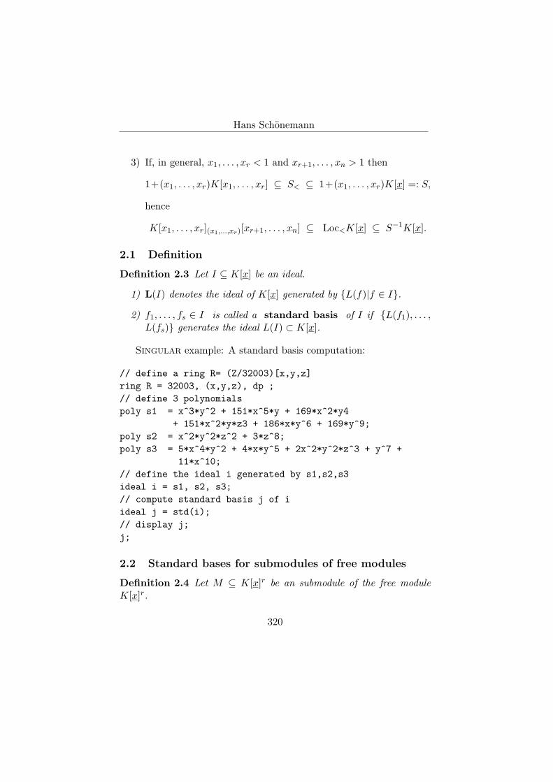
3) If, in general, x1, . . . , xr < 1 and xr+1, . . . , xn > 1 then

1+(x1, . . . , xr)K[x1, . . . , xr] ⊆ S< ⊆ 1+(x1, . . . , xr)K[x] =: S,

hence

K[x1, . . . , xr](x1,...,xr)[xr+1, . . . , xn] ⊆ Loc<K[x] ⊆ S−1K[x].

2.1 Definition

Definition 2.3 Let I ⊆ K[x] be an ideal.

1) L(I) denotes the ideal of K[x] generated by L(f)|f ∈ I.2) f1, . . . , fs ∈ I is called a standard basis of I if L(f1), . . . ,

L(fs) generates the ideal L(I) ⊂ K[x].

Singular example: A standard basis computation:

// define a ring R= (Z/32003)[x,y,z]ring R = 32003, (x,y,z), dp ;// define 3 polynomialspoly s1 = x^3*y^2 + 151*x^5*y + 169*x^2*y4

+ 151*x^2*y*z3 + 186*x*y^6 + 169*y^9;poly s2 = x^2*y^2*z^2 + 3*z^8;poly s3 = 5*x^4*y^2 + 4*x*y^5 + 2x^2*y^2*z^3 + y^7 +

11*x^10;// define the ideal i generated by s1,s2,s3ideal i = s1, s2, s3;// compute standard basis j of iideal j = std(i);// display j;j;

2.2 Standard bases for submodules of free modules

Definition 2.4 Let M ⊆ K[x]r be an submodule of the free moduleK[x]r.

320

Algorithms in Singular

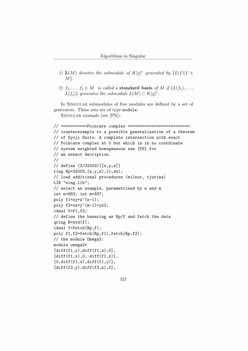
1) L(M) denotes the submodule of K[x]r generated by L(f)|f ∈M.

2) f1, . . . , fs ∈ M is called a standard basis of M if L(f1), . . . ,L(fs) generates the submodule L(M) ⊂ K[x]r.

In Singular submodules of free modules are defined by a set ofgenerators. These sets are of type module.

Singular example (see [PS]):

// ===========Poincare complex ==========================// counterexample to a possible generalization of a theorem// of Kyoji Saito. A complete intersection with exact// Poincare complex at 0 but which is in no coordinate// system weighted homogeneous see [PS] for// an exeact decription.//// define (Z/32003)[[x,y,z]]ring Rp=32003,(x,y,z),(c,ds);// load additional procedures (milnor, tjurina)LIB "sing.lib";// select an example, parametrized by n and mint n=883; int m=937;poly f1=xy+z^(n-1);poly f2=xz+y^(m-1)+yz2;ideal f=f1,f2;// define the basering as Rp/f and fetch the dataqring R=std(f);ideal f=fetch(Rp,f);poly f1,f2=fetch(Rp,f1),fetch(Rp,f2);// the module Omega2:module omega2=[diff(f1,y),diff(f1,z),0],[diff(f1,x),0,-diff(f1,z)],[0,diff(f1,x),diff(f1,y)],[diff(f2,y),diff(f2,z),0],

321

Hans Schonemann

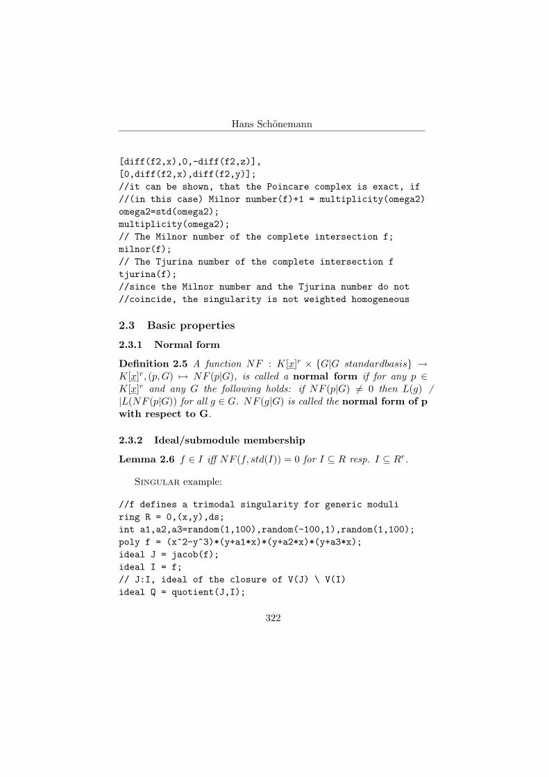
[diff(f2,x),0,-diff(f2,z)],[0,diff(f2,x),diff(f2,y)];//it can be shown, that the Poincare complex is exact, if//(in this case) Milnor number(f)+1 = multiplicity(omega2)omega2=std(omega2);multiplicity(omega2);// The Milnor number of the complete intersection f;milnor(f);// The Tjurina number of the complete intersection ftjurina(f);//since the Milnor number and the Tjurina number do not//coincide, the singularity is not weighted homogeneous

2.3 Basic properties

2.3.1 Normal form

Definition 2.5 A function NF : K[x]r × G|G standardbasis →K[x]r, (p, G) 7→ NF (p|G), is called a normal form if for any p ∈K[x]r and any G the following holds: if NF (p|G) 6= 0 then L(g) 6|L(NF (p|G)) for all g ∈ G. NF (g|G) is called the normal form of pwith respect to G.

2.3.2 Ideal/submodule membership

Lemma 2.6 f ∈ I iff NF (f, std(I)) = 0 for I ⊆ R resp. I ⊆ Rr.

Singular example:

//f defines a trimodal singularity for generic moduliring R = 0,(x,y),ds;int a1,a2,a3=random(1,100),random(-100,1),random(1,100);poly f = (x^2-y^3)*(y+a1*x)*(y+a2*x)*(y+a3*x);ideal J = jacob(f);ideal I = f;// J:I, ideal of the closure of V(J) \ V(I)ideal Q = quotient(J,I);

322

Algorithms in Singular

//the Hessian of fpoly Hess = det(jacob(jacob(f)));//Hess is contained in Q iff NF is 0reduce(Hess,std(Q));

2.3.3 Elimination

Lemma 2.7 Let < be an elimination order for y1, . . . , yn, R =K[x1, . . . , xr, y1, . . . , yn].Then std(I) ∩K[x1, . . . , xr] = std(I ∩K[x1, . . . , xr]).

Singular example:

// find the equations from a parametrization// t->(t^3,t^4,t^5)ring R=0,(x,y,z,t),dp;ideal i=x-t^3,

y-t^4,z-t^5;

ideal j=eliminate(i,t);j;

Remark 2.8 The elimination property applies also to modules.

2.3.4 Hilbert series

Definition 2.9 Let M be a graded module over K[x]. The Hilbertseries of M is the power series

H(M)(t) =∞∑

t=−∞dimKMit

i

.

Lemma 2.10 Let < be a (positive or negative) degree ordering andH(M) the Hilbert function of (the homogenization of) I. Then H(M) =H(L(M)).

323

Hans Schonemann

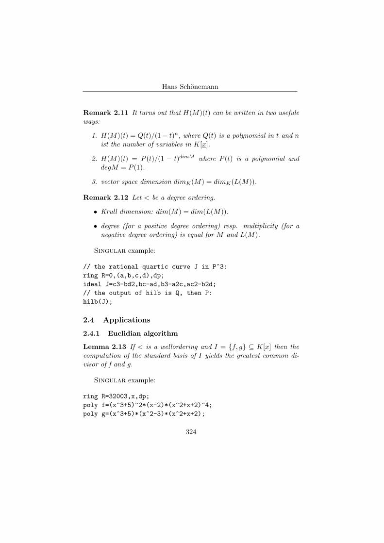
Remark 2.11 It turns out that H(M)(t) can be written in two usefuleways:

1. H(M)(t) = Q(t)/(1− t)n, where Q(t) is a polynomial in t and nist the number of variables in K[x].

2. H(M)(t) = P (t)/(1 − t)dimM where P (t) is a polynomial anddegM = P (1).

3. vector space dimension dimK(M) = dimK(L(M)).

Remark 2.12 Let < be a degree ordering.

• Krull dimension: dim(M) = dim(L(M)).

• degree (for a positive degree ordering) resp. multiplicity (for anegative degree ordering) is equal for M and L(M).

Singular example:

// the rational quartic curve J in P^3:ring R=0,(a,b,c,d),dp;ideal J=c3-bd2,bc-ad,b3-a2c,ac2-b2d;// the output of hilb is Q, then P:hilb(J);

2.4 Applications

2.4.1 Euclidian algorithm

Lemma 2.13 If < is a wellordering and I = f, g ⊆ K[x] then thecomputation of the standard basis of I yields the greatest common di-visor of f and g.

Singular example:

ring R=32003,x,dp;poly f=(x^3+5)^2*(x-2)*(x^2+x+2)^4;poly g=(x^3+5)*(x^2-3)*(x^2+x+2);

324

Algorithms in Singular

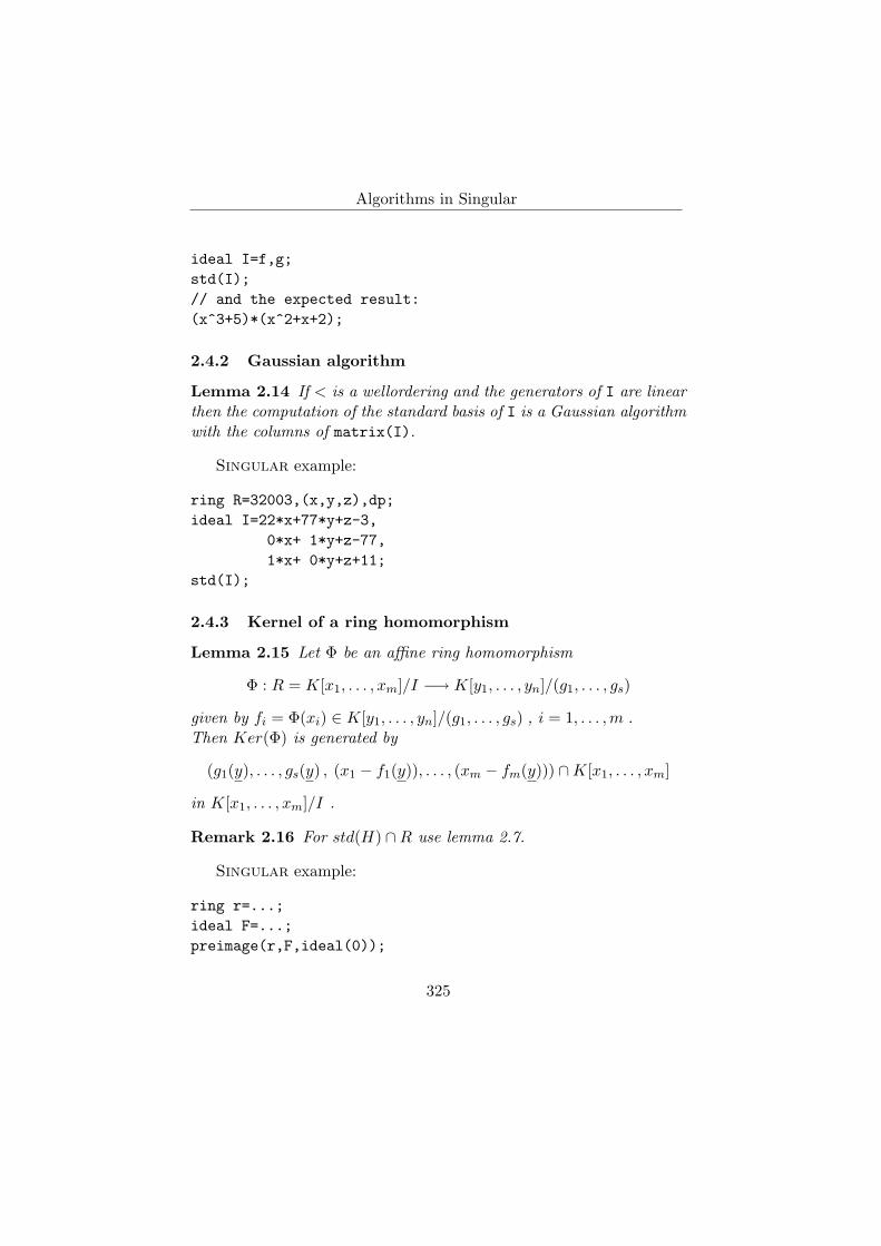
ideal I=f,g;std(I);// and the expected result:(x^3+5)*(x^2+x+2);

2.4.2 Gaussian algorithm

Lemma 2.14 If < is a wellordering and the generators of I are linearthen the computation of the standard basis of I is a Gaussian algorithmwith the columns of matrix(I).

Singular example:

ring R=32003,(x,y,z),dp;ideal I=22*x+77*y+z-3,

0*x+ 1*y+z-77,1*x+ 0*y+z+11;

std(I);

2.4.3 Kernel of a ring homomorphism

Lemma 2.15 Let Φ be an affine ring homomorphism

Φ : R = K[x1, . . . , xm]/I −→ K[y1, . . . , yn]/(g1, . . . , gs)

given by fi = Φ(xi) ∈ K[y1, . . . , yn]/(g1, . . . , gs) , i = 1, . . . ,m .Then Ker(Φ) is generated by

(g1(y), . . . , gs(y) , (x1 − f1(y)), . . . , (xm − fm(y))) ∩K[x1, . . . , xm]

in K[x1, . . . , xm]/I .

Remark 2.16 For std(H) ∩R use lemma 2.7.

Singular example:

ring r=...;ideal F=...;preimage(r,F,ideal(0));

325

Hans Schonemann

2.4.4 Radical membership

Lemma 2.17 Let I ⊆ R = Loc<K[x1, . . . , xn], I generated by F .f ∈ √I iff 1 ∈ std(F + (yf − 1) ⊆ R[y].

2.4.5 Principal ideal

Lemma 2.18 I = (F ) is principal (i.e. has a one-element ideal basis)iff std(F ) has exactly one element.

2.4.6 Trivial ideal

Lemma 2.19 (F ) is the whole ring R iff std(F ) = 1.

2.4.7 Intersection 1

Lemma 2.20 Let (F ) ⊆ Rr and (G) ⊆ Rr.Then std((F ) ∩ (G)) = std(y(F ) + (1− y)(G)) ∩R in R[y].

Remark 2.21 For std(H) ∩R use lemma 2.7.

Singular example:

ring r1 = 32003,(x,y,z),(c,ds);poly s1=x2y3+45x6y3+68x4z5+80y6x8;poly s2=6x5+3y6+8z6;poly s3=12xyz3+2y3z6;ideal i1=s1,s2,s3;ideal i2=s1+s2,s2,s1;intersect(i1,i2);

2.4.8 Ideal/module quotient 1

Lemma 2.22 Let (F ) ⊆ Rr, g ∈ Rr.Then (F ) : (g) = (h1, . . . , hk) if (F ) ∩ (g)) = (h1g, . . . , hkg).

Lemma 2.23 Let (F ) ⊆ Rr, (g1, . . . , gs) ∈ Rr.Then (F ) : (g1, . . . , gs) = (F ) : (g1) ∩ . . . ∩ (F ) : (gs).

Remark 2.24 Singular uses another algorithm, see 4.8.

326

Algorithms in Singular

2.4.9 Saturation 1

Lemma 2.25 Let (F ) ⊆ Rr, g ∈ Rr.Then (F ) : (g)∞ = (h1, . . . , hk) if (F ) ∩ (g)) = (h1g, . . . , hkg).

Remark 2.26 Singular uses another algorithm, see 4.9

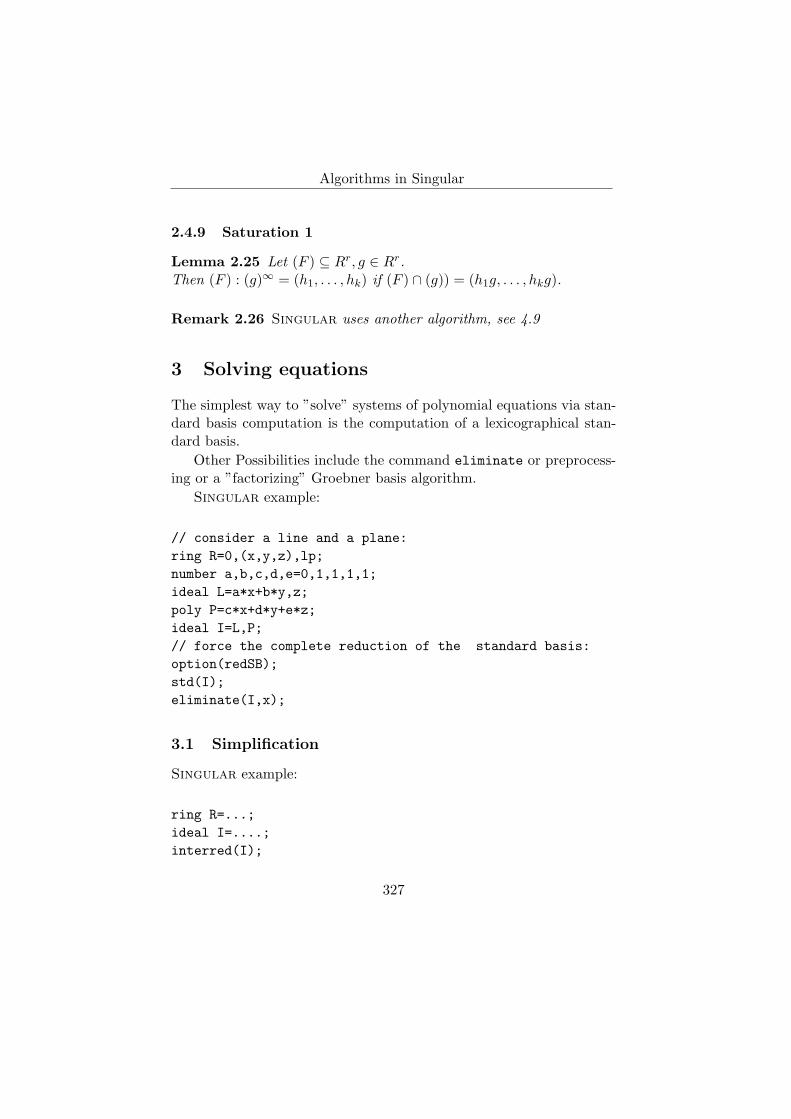
3 Solving equations

The simplest way to ”solve” systems of polynomial equations via stan-dard basis computation is the computation of a lexicographical stan-dard basis.

Other Possibilities include the command eliminate or preprocess-ing or a ”factorizing” Groebner basis algorithm.

Singular example:

// consider a line and a plane:ring R=0,(x,y,z),lp;number a,b,c,d,e=0,1,1,1,1;ideal L=a*x+b*y,z;poly P=c*x+d*y+e*z;ideal I=L,P;// force the complete reduction of the standard basis:option(redSB);std(I);eliminate(I,x);

3.1 Simplification

Singular example:

ring R=...;ideal I=....;interred(I);

327

Hans Schonemann

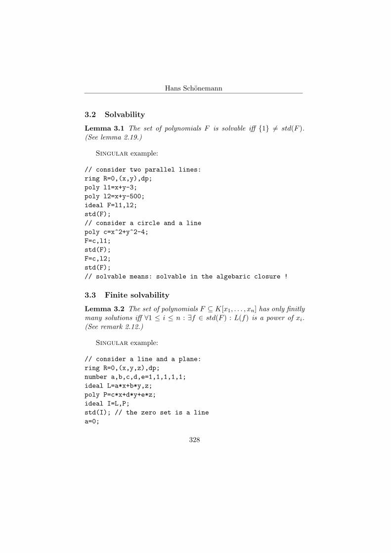
3.2 Solvability

Lemma 3.1 The set of polynomials F is solvable iff 1 6= std(F ).(See lemma 2.19.)

Singular example:

// consider two parallel lines:ring R=0,(x,y),dp;poly l1=x+y-3;poly l2=x+y-500;ideal F=l1,l2;std(F);// consider a circle and a linepoly c=x^2+y^2-4;F=c,l1;std(F);F=c,l2;std(F);// solvable means: solvable in the algebaric closure !

3.3 Finite solvability

Lemma 3.2 The set of polynomials F ⊆ K[x1, . . . , xn] has only finitlymany solutions iff ∀1 ≤ i ≤ n : ∃f ∈ std(F ) : L(f) is a power of xi.(See remark 2.12.)

Singular example:

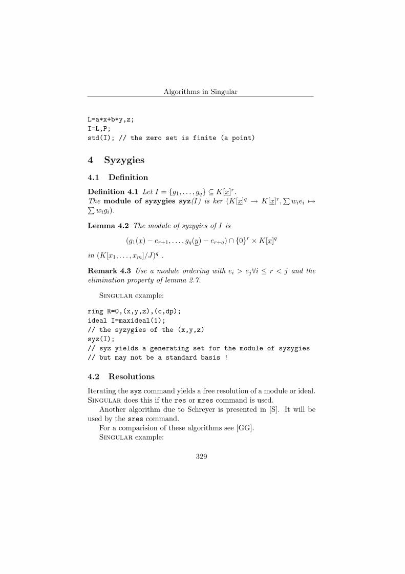
// consider a line and a plane:ring R=0,(x,y,z),dp;number a,b,c,d,e=1,1,1,1,1;ideal L=a*x+b*y,z;poly P=c*x+d*y+e*z;ideal I=L,P;std(I); // the zero set is a linea=0;

328

Algorithms in Singular

L=a*x+b*y,z;I=L,P;std(I); // the zero set is finite (a point)

4 Syzygies

4.1 Definition

Definition 4.1 Let I = g1, . . . , gq ⊆ K[x]r.The module of syzygies syz(I) is ker (K[x]q → K[x]r,

∑wiei 7→∑

wigi).

Lemma 4.2 The module of syzygies of I is

(g1(x)− er+1, . . . , gq(y)− er+q) ∩ 0r ×K[x]q

in (K[x1, . . . , xm]/J)q .

Remark 4.3 Use a module ordering with ei > ej∀i ≤ r < j and theelimination property of lemma 2.7.

Singular example:

ring R=0,(x,y,z),(c,dp);ideal I=maxideal(1);// the syzygies of the (x,y,z)syz(I);// syz yields a generating set for the module of syzygies// but may not be a standard basis !

4.2 Resolutions

Iterating the syz command yields a free resolution of a module or ideal.Singular does this if the res or mres command is used.

Another algorithm due to Schreyer is presented in [S]. It will beused by the sres command.

For a comparision of these algorithms see [GG].Singular example:

329

Hans Schonemann

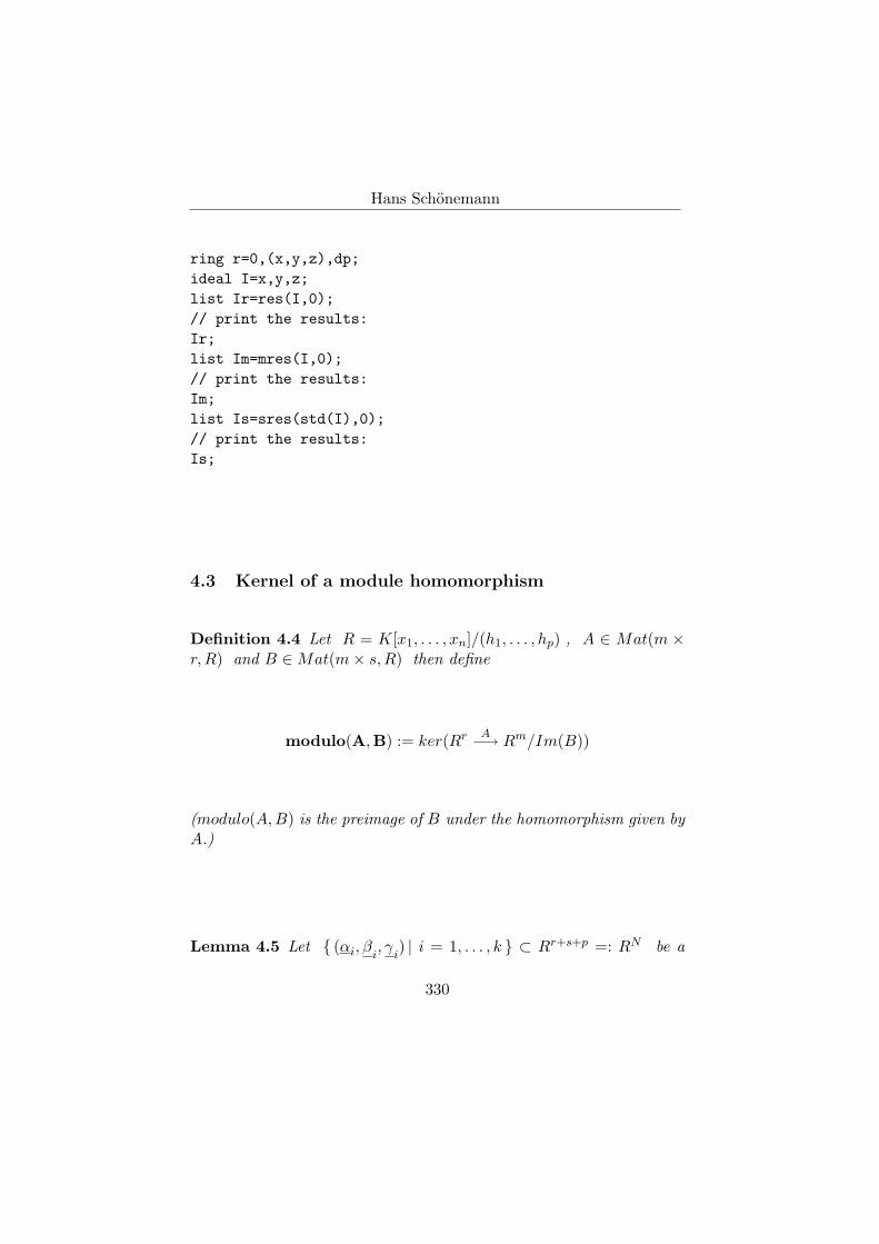
ring r=0,(x,y,z),dp;ideal I=x,y,z;list Ir=res(I,0);// print the results:Ir;list Im=mres(I,0);// print the results:Im;list Is=sres(std(I),0);// print the results:Is;

4.3 Kernel of a module homomorphism

Definition 4.4 Let R = K[x1, . . . , xn]/(h1, . . . , hp) , A ∈ Mat(m ×r,R) and B ∈ Mat(m× s,R) then define

modulo(A,B) := ker(Rr A−→ Rm/Im(B))

(modulo(A, B) is the preimage of B under the homomorphism given byA.)

Lemma 4.5 Let (αi, βi, γ

i) | i = 1, . . . , k ⊂ Rr+s+p =: RN be a

330

Algorithms in Singular

generating set of syz(D) where

C =

h1 · · · hp 0 · · · · · · · · · · · · · · ·0 · · · 0 h1 · · · hp 0 · · · · · ·...

...0 · · · · · · · · · · · · · · · h1 · · · hp

∈

Mat(m× pm,R)

and

D =

a11 · · · a1r b11 · · · b1s c11 · · · c1,pm...

......

......

...am1 · · · amr bm1 · · · bms cm1 · · · cm,pm

∈

Mat(m× r + s + pm,R)

Then

modulo (A,B) := ( α1 . . . αk ) ∈ Mat(r × k, R)

(see lemma 4.2.)

Remark 4.6 In practice, one need not compute the entire syzygy mod-ule of D: it is better to find modulo(A,B) as:

a11 · · · a1r b11 · · · b1s c11 · · · c1,pm...

......

......

...am1 · · · amr bm1 · · · bms cm1 · · · cm,pm

1 0 0 · · · · · · · · · · · · 00 . . . 0 0 · · · · · · · · · · · · 00 1 0 · · · · · · · · · · · · 0

∩

0...0R...R

(see sections 4.2, 2.7.)

331

Hans Schonemann

4.4 Module intersection 2

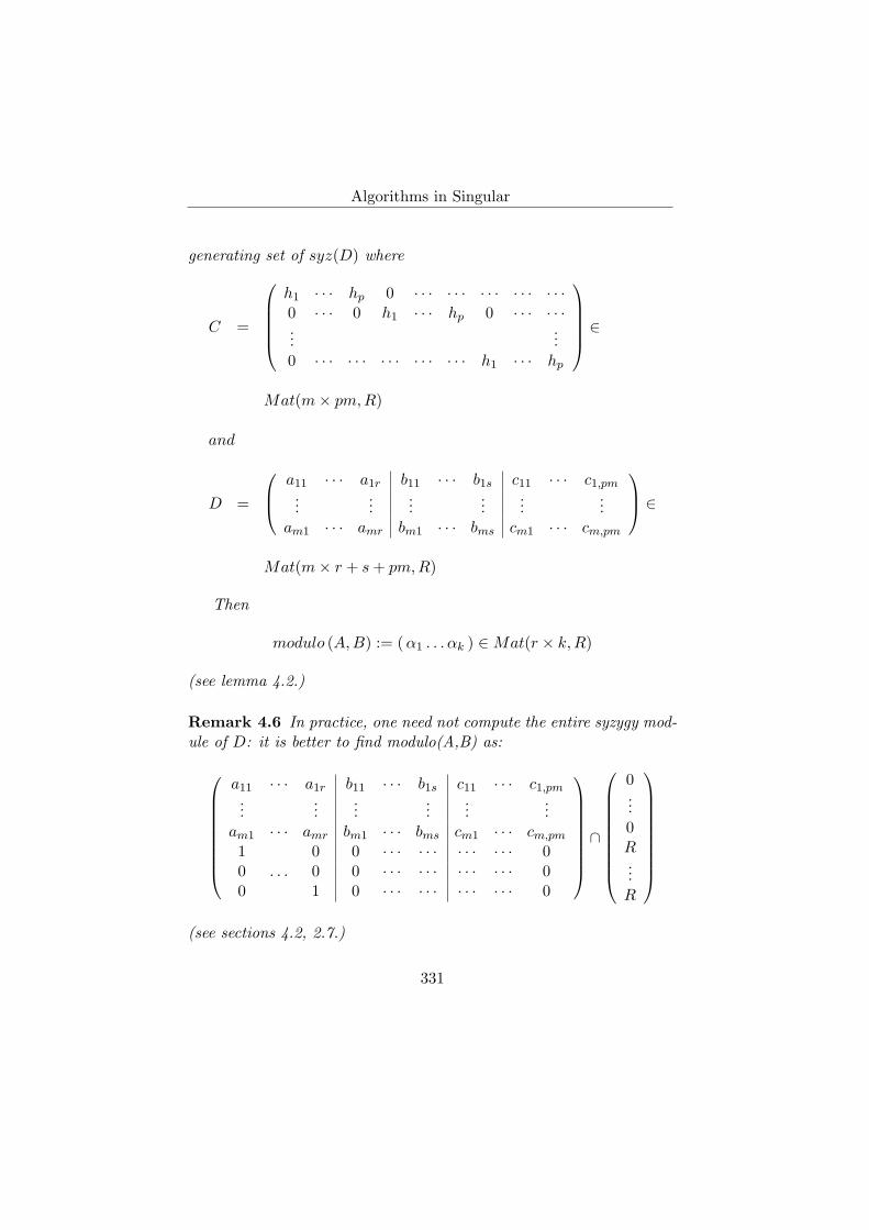
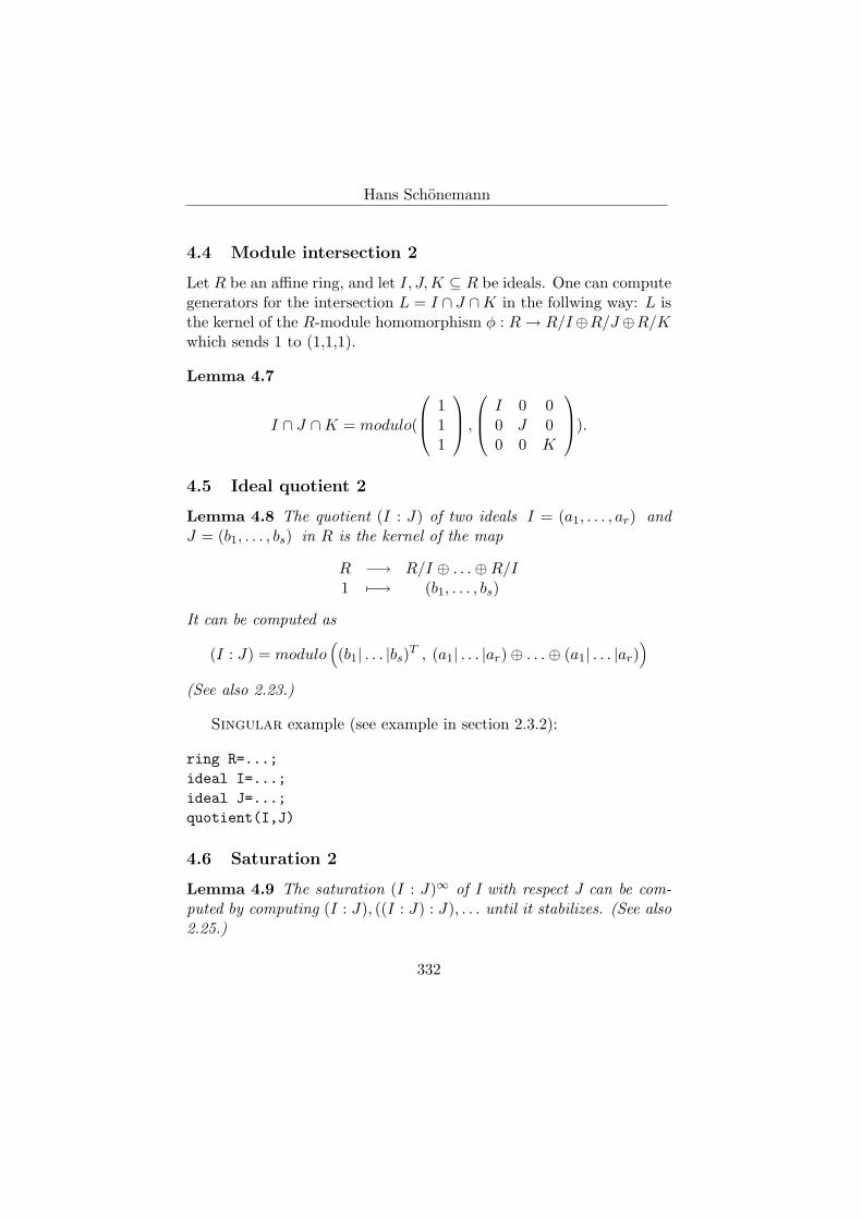
Let R be an affine ring, and let I, J,K ⊆ R be ideals. One can computegenerators for the intersection L = I ∩ J ∩K in the follwing way: L isthe kernel of the R-module homomorphism φ : R → R/I⊕R/J⊕R/Kwhich sends 1 to (1,1,1).

Lemma 4.7

I ∩ J ∩K = modulo(

111

,

I 0 00 J 00 0 K

).

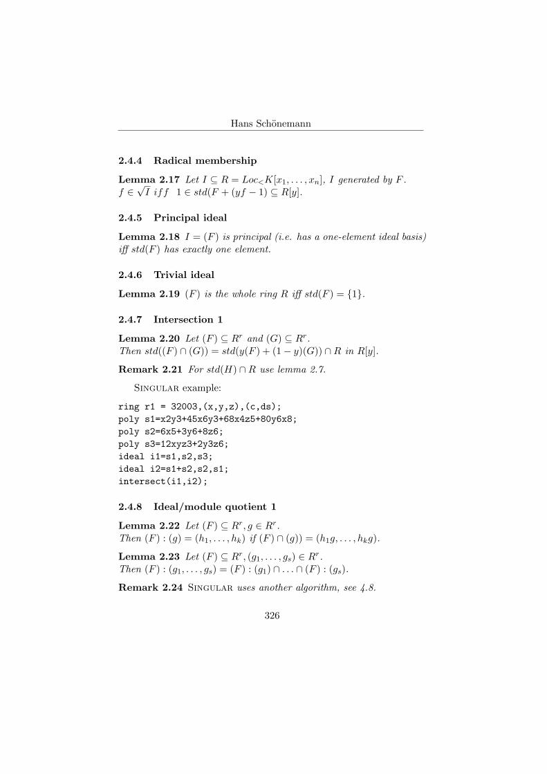
4.5 Ideal quotient 2

Lemma 4.8 The quotient (I : J) of two ideals I = (a1, . . . , ar) andJ = (b1, . . . , bs) in R is the kernel of the map

R −→ R/I ⊕ . . .⊕R/I1 7−→ (b1, . . . , bs)

It can be computed as

(I : J) = modulo((b1| . . . |bs)T , (a1| . . . |ar)⊕ . . .⊕ (a1| . . . |ar)

)

(See also 2.23.)

Singular example (see example in section 2.3.2):

ring R=...;ideal I=...;ideal J=...;quotient(I,J)

4.6 Saturation 2

Lemma 4.9 The saturation (I : J)∞ of I with respect J can be com-puted by computing (I : J), ((I : J) : J), . . . until it stabilizes. (See also2.25.)

332

Algorithms in Singular

Singular example:

ring R=...;ideal I=...;ideal J=...;int ii;I = std(I);while ( ii<=size(II))II=quotient(I,J);for ( ii=1; ii <=size(II); ii=ii++)if (reduce(II[ii],I)!=0) break;

I=std(II);

// II is now (I:J)∞.

4.7 Annihilator of a module

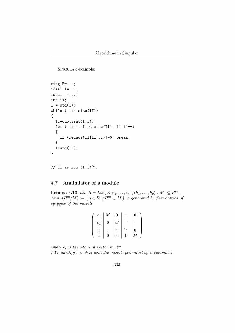
Lemma 4.10 Let R = Loc<K[x1, . . . , xn]/(h1, . . . , hp) , M ⊆ Rm.AnnR(Rm/M) := g ∈ R | gRm ⊂ M is generated by first entries ofsyzygies of the module

e1 M 0 · · · 0

e2 0 M. . .

......

.... . . . . . 0

em 0 · · · 0 M

where ei is the i-th unit vector in Rm.(We identify a matrix with the module generated by it columns.)

333

Hans Schonemann

5 Examples

5.1 Ext modules Ext(M,R)

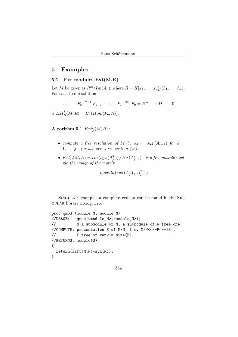
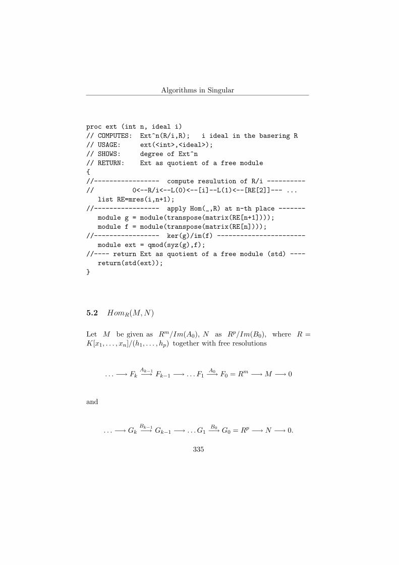
Let M be given as Rm/Im(A0), where R = K[x1, . . . , xn]/(h1, . . . , hp) .For each free resolution

. . . −→ FkAk−1−→ Fk−1 −→ . . . F1

A0−→ F0 = Rm −→ M −→ 0

is ExtjR(M, R) = Hj(Hom(F•, R)).

Algorithm 5.1 ExtjR(M,R) :

• compute a free resolution of M by Ak = syz (Ak−1) for k =1, . . . , j . (or use mres, see section 4.2).

• ExtjR(M,R) = Im (syz (ATj )) /Im (AT

j−1) is a free module mod-ulo the image of the matrix

modulo (syz (ATj ) , AT

j−1)

Singular example: a complete version can be found in the Sin-gular library homog.lib.

proc qmod (module M, module N)//USAGE: qmod(<module_M>,<module_N>);// N a submodule of M, a submodule of a free one//COMPUTE: presentation S of M/N, i.e. M/N<<--F<--[S],// F free of rank = size(M),//RETURNS: module(S)return(lift(M,N)+syz(M));

334

Algorithms in Singular

proc ext (int n, ideal i)// COMPUTES: Ext^n(R/i,R); i ideal in the basering R// USAGE: ext(<int>,<ideal>);// SHOWS: degree of Ext^n// RETURN: Ext as quotient of a free module//----------------- compute resulution of R/i ----------// 0<--R/i<--L(0)<--[i]--L(1)<--[RE[2]]--- ...

list RE=mres(i,n+1);//----------------- apply Hom(_,R) at n-th place -------

module g = module(transpose(matrix(RE[n+1])));module f = module(transpose(matrix(RE[n])));

//----------------- ker(g)/im(f) -----------------------module ext = qmod(syz(g),f);

//---- return Ext as quotient of a free module (std) ----return(std(ext));

5.2 HomR(M,N)

Let M be given as Rm/Im(A0), N as Rp/Im(B0), where R =K[x1, . . . , xn]/(h1, . . . , hp) together with free resolutions

. . . −→ FkAk−1−→ Fk−1 −→ . . . F1

A0−→ F0 = Rm −→ M −→ 0

and

. . . −→ GkBk−1−→ Gk−1 −→ . . . G1

B0−→ G0 = Rp −→ N −→ 0.

335

Hans Schonemann

We get the following commutative diagram with exact columns androws:

0↓

HomR(M, N)↓

0 ←− F ∗0 ⊗N ←− F ∗

0 ⊗G0 ←− F ∗0 ⊗G1

↓ ↓ ↓0 ←− F ∗

1 ⊗N ←− F ∗1 ⊗G0 ←− F ∗

1 ⊗G1

.

Algorithm 5.2

HomR(M,N) = Im (modulo (AT0 ⊗ idG0 , idF ∗1 ⊗B0)) / Im (idF ∗0 ⊗B0)

is a free module modulo the image of the matrix

modulo (modulo (AT0 ⊗ idG0 , idF ∗1 ⊗B0) , idF ∗0 ⊗B0)

5.3 T 1X and T 1

X(M)

This section and the corresponding Singular procedure is a joint workof G.M. Greuel and B.Martin.

Let X ∈ Kn be given by the ideal I = (f1, . . . , fk) ⊆ P =K[x1, . . . , xn] and R = P/I.

Consider the canonical exact sequence

I/I2 d−→ Ω1P ⊗P R −→ Ω1

R → 0 (1)

336

Algorithms in Singular

where Ω1P denotes the module of Kahler differentials and d is induced

by the exterior derivation. ([d] 7→ [df ]).Ω1

P is free with generators dx1, . . . , dxn (isomorph to Pn) and Ω1R

(isomorph to Rn) is by definition the cokernel of the map

d : [fi] → [dfi] = [∑

j

(dfi/dxj)]

Let M be any finitely generated R-module . The M -dual of (1) is

0 → ΘX(M) → HomR(ΩP⊗R, M) d∗−→ HomR(I/I2,M) → T 1X(M) → 0

where ΘX(M) = HomR(Ω1R,M) is the module of the M -valued R-

derivations and T 1X(M) is by definition the cokernel of d∗ (the dual of d)

and is called the module of first order infinitesimal deformationsof X (resp. R) with values in M .

The module T 1X/Kn(M) := HomR(I/I2,M) is called the module

of first order embedded deformations of R with values in M . IfM is ommitted, we define T 1

X := T 1X(R) as the module of first order

deformations of X.Remark: HomR(Ω1

R, R) ∼= HomP (Rn, R) ∼= Rn.

Algorithm 5.3 Consider a presentation of I as a P -module:

0 ← I ← P k A←− P p (2)

We note that for any R-module M

HomP (I/I2,M) = HomR(I, M) (3)

Hence, choosing dx1, . . . , dxn as a basis of Ω1P and the canonical basis

of P k, the right part of (3) is identified with the exact sequence

HomP (Pn, R)jac−→ HomP (I, M) → T 1

X(M) → 0 (4)

where jac : HomP (Pn, M) → HomP (I, M) ⊆ HomP (P k,M) = Mk

is given by the Jacobian matrix (dfi/dxj)i,j of I. In particuliar, forM = R, we get

HomP (Pn, R)jac−→ HomP (I,R) → T 1

X → 0 (5)

337

Hans Schonemann

as defining sequence of T 1X .

Applying HomP (−, R) to (2), we get

0 → HomP (I, R) = ker(A∗) → HomP (P k, R) A∗−→ HomP (P p, R) (6)

where A∗ is the transposed matrix of A. Consider a 3-term partialresolution of im(A∗):

Rq B3−→ Rr B2−→ HomP (P k, R) B1:=A∗−→ HomP (P p, R) (7)

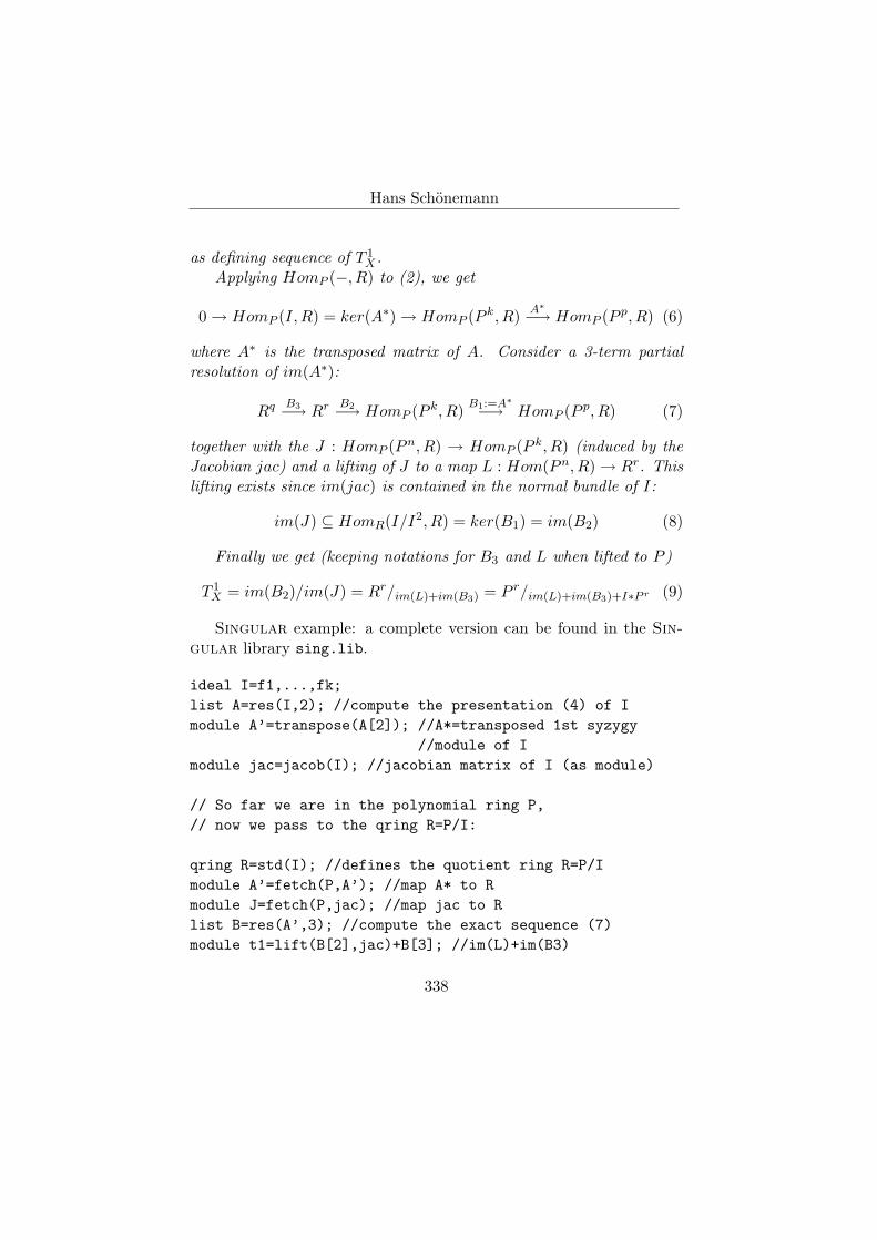
together with the J : HomP (Pn, R) → HomP (P k, R) (induced by theJacobian jac) and a lifting of J to a map L : Hom(Pn, R) → Rr. Thislifting exists since im(jac) is contained in the normal bundle of I:

im(J) ⊆ HomR(I/I2, R) = ker(B1) = im(B2) (8)

Finally we get (keeping notations for B3 and L when lifted to P )

T 1X = im(B2)/im(J) = Rr/im(L)+im(B3) = P r/im(L)+im(B3)+I∗P r (9)

Singular example: a complete version can be found in the Sin-gular library sing.lib.

ideal I=f1,...,fk;list A=res(I,2); //compute the presentation (4) of Imodule A’=transpose(A[2]); //A*=transposed 1st syzygy

//module of Imodule jac=jacob(I); //jacobian matrix of I (as module)

// So far we are in the polynomial ring P,// now we pass to the qring R=P/I:

qring R=std(I); //defines the quotient ring R=P/Imodule A’=fetch(P,A’); //map A* to Rmodule J=fetch(P,jac); //map jac to Rlist B=res(A’,3); //compute the exact sequence (7)module t1=lift(B[2],jac)+B[3]; //im(L)+im(B3)

338

Algorithms in Singular

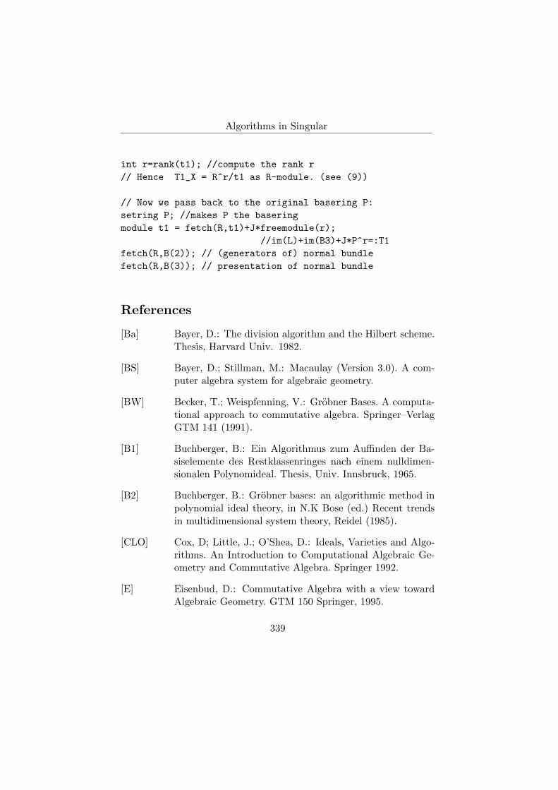
int r=rank(t1); //compute the rank r// Hence T1_X = R^r/t1 as R-module. (see (9))

// Now we pass back to the original basering P:setring P; //makes P the baseringmodule t1 = fetch(R,t1)+J*freemodule(r);

//im(L)+im(B3)+J*P^r=:T1fetch(R,B(2)); // (generators of) normal bundlefetch(R,B(3)); // presentation of normal bundle

References

[Ba] Bayer, D.: The division algorithm and the Hilbert scheme.Thesis, Harvard Univ. 1982.

[BS] Bayer, D.; Stillman, M.: Macaulay (Version 3.0). A com-puter algebra system for algebraic geometry.

[BW] Becker, T.; Weispfenning, V.: Grobner Bases. A computa-tional approach to commutative algebra. Springer–VerlagGTM 141 (1991).

[B1] Buchberger, B.: Ein Algorithmus zum Auffinden der Ba-siselemente des Restklassenringes nach einem nulldimen-sionalen Polynomideal. Thesis, Univ. Innsbruck, 1965.

[B2] Buchberger, B.: Grobner bases: an algorithmic method inpolynomial ideal theory, in N.K Bose (ed.) Recent trendsin multidimensional system theory, Reidel (1985).

[CLO] Cox, D; Little, J.; O’Shea, D.: Ideals, Varieties and Algo-rithms. An Introduction to Computational Algebraic Ge-ometry and Commutative Algebra. Springer 1992.

[E] Eisenbud, D.: Commutative Algebra with a view towardAlgebraic Geometry. GTM 150 Springer, 1995.

339

Hans Schonemann

[G] Grabe, H.-G.: The tangent cone algorithm and homoge-nization. To appear in J. Pure Appl. Alg.

[GG] Grassmann, H; Greuel, G.-M.; Martin, B.; Neumann, W.;Pfister, G.; Pohl, W.; Schonemann, H.; Siebert, T.: Stan-dard bases, syzygies and their implementation in SINGU-LAR. Preprint 251, Fachbereich Mathematik, UniversitatKaiserslautern 1994.

[GM] Gebauer, R.; Moller, M.: On an installation of Buch-berger’s Algorithm. J. Symbolic Computation (1988) 6,275–286.

[GMNRT] Giovini, A.; Mora, T.; Niesi, G.; Robbiano, L.; Traverso,C.: “One sugar cube, please” or selection strategies in theBuchberger algorithm. Proceedings of the 1991 ISSAC, 55-63.

[GTZ] Gianni, P.; Trager, B.;Zacharias, G.: Grobner bases andPrimary Decomposition of Polynomial Ideals. Journal ofSymbolic Computation. 1985.

[L] Lazard, D.: Grobner bases, Gaussian elimination, and res-olution of systems of algebraic equations. Proc. EUROCAL83, LN Comp. Sci. 162, 146–156.

[M1] Mora, T.: An algorithm to compute the equations of tan-gent cones. Proc. EUROCAM 82, Springer Lecture Notesin Computer Science (1982).

[M2] Mora, T.: Seven variations on standard bases. Preprint,Univ. Genova (1988).

[M3] Mora, T.: La Queste del Saint Graal: a computationalapproach to local algebra. Discrete Applied Math. 33, 161-190 (1991).

[MMT] Moller, H.M.; Mora, T.; Traverso, C.: Grobner bases com-putation using syzygies. Proc. of ISSAC 1992.

340

Algorithms in Singular

[MPT] Mora, T.; Pfister, G.; Traverso, C.: An introduction tothe tangent cone algorithm . Advances in Computing re-search, Issues in Robotics and nonlinear geometry (6) 199–270 (1992).

[PS] Pfister, G.; Schonemann, H.: Singularities with exactPoincare complex but not quasihomogeneous. Rev. Mat.de la Univ. Complutense de Madrid 2 (1989).

[R] Robbiano, L.: Termorderings on the polynomial ring. Pro-ceedings of EUROCAL 85, Lecture Notes in Computer Sci-ence 204, 513–517 (1985).

[S] Schreyer, F.-O.: A standard basis approach to syzygies ofcanonical curves. J. reine angew. Math. 421, 83-123 (1991).

[St1] Stillman, M.: Methods for computing in algebraic geom-etry and commutative algebra. Acta Applicandae Mathe-maticae 21(77-103) 1990.

[St2] Stillman, M.: Macaulay. A tutorial. 1992.

[Si] Singular reference manual. Version 0.9.2. 1995. Availablefrom ftp://helios.mathematik.uni-kl.de/pub/Math/Singular/bin

Hannes Schonemann, Received 27 November, 1996Department of Mathematics,University of KaiserslauternGermanye-mail: hannes@mathematik.uni− kl.de

341