ALMA MATER STUDIORUM - UNIVERSITÀ DI BOLOGNA FACOLTA’ DI INGEGNERIA INTERNATIONAL MASTER COURSE IN CIVIL ENGINEERING Dipartimento di Ingegneria Civile, Ambientale e dei Materiali TESI DI LAUREA in Earthquake Engineering PUSHOVER ANALYSIS OF AN EXISTING REINFORCED CONCRETE BRIDGE: THE JAMBOREE ROAD OVERCROSSING IN IRVINE, CALIFORNIA CANDIDATO RELATORE: Giulia Cavallari Chiar.mo Prof. Marco Savoia CORRELATORI Dott. Ing. Nicola Buratti Dott. Ing. Hugo C. Gomez Anno Accademico 2010/2011 Sessione III
Transcript
ALMA MATER STUDIORUM - UNIVERSITÀ DI BOLOGNA
FACOLTA’ DI INGEGNERIA
INTERNATIONAL MASTER COURSE IN CIVIL ENGINEERING
Dipartimento di Ingegneria Civile, Ambientale e dei Materiali
TESI DI LAUREA
in Earthquake Engineering
PUSHOVER ANALYSIS OF AN EXISTING REINFORCED
CONCRETE BRIDGE:
THE JAMBOREE ROAD OVERCROSSING
IN IRVINE, CALIFORNIA
CANDIDATO RELATORE: Giulia Cavallari Chiar.mo Prof. Marco Savoia CORRELATORI Dott. Ing. Nicola Buratti
Dott. Ing. Hugo C. Gomez
Anno Accademico 2010/2011
Sessione III
Alla mia famiglia.
Index
Introduction ………………………………………………..…………………..1
1. Nonlinear analysis in seismic design of bridges………………...…3 1.1. Seismic design philosophy for bridges: capacity design ………….….5
1.1.1. Performance level………………..………..…………………..6 1.1.2. Seismic capacity…………………………..…………………..6 1.1.3. Ductility and predetermined location of damage……………..8
1.2. Types of nonlinear analyses…………………………………………..9
1.3.1. Earthquake ground shaking hazard levels (ATC 40) ..……...13 1.3.2. Development of the design spectrum (SDC 2010, Annex B).13 1.3.3. Acceleration time-history (FEMA 273)……………………..18
2. Finite element models for the nonlinear material response of beam-column elements: formulations and objectivity of the response……………………………………………………...………….....25 2.1. Concentrated plasticity models, force-based formulation…………...28
2.1.1. Element Formulation (Scott et al. 1996) …………………....28 2.1.2. Loss of objectivity in force-based beam-column elements….31 2.1.3. Plastic hinge integration methods…………………………...33 2.1.4. Plastic hinge length determination (Priestley, Calvi, Seible,
2.2.1. Element Formulation (Spacone et al. 1996) …………….…..41 2.2.2. Element and Section state determination…………….….…..44 2.2.3. Numerical integration…………….….…..………...….….….48 2.2.4. Loss of objectivity at section and element levels (Coleman and
3. Existing structure and modeling issues …………………...…….....55 3.1. The existing structure: Jamboree Road Overcrossing…………….....55
3.2. The OpenSees modeling……………….....……………….................58
3.2.1. The software OpenSees……………….....………………......58 3.2.2. The Three-Dimensional Model……………...........................60 3.2.3. Modal Analysis and the definition of the load path for the
Pushover Analysis…………….....…………….....………….63
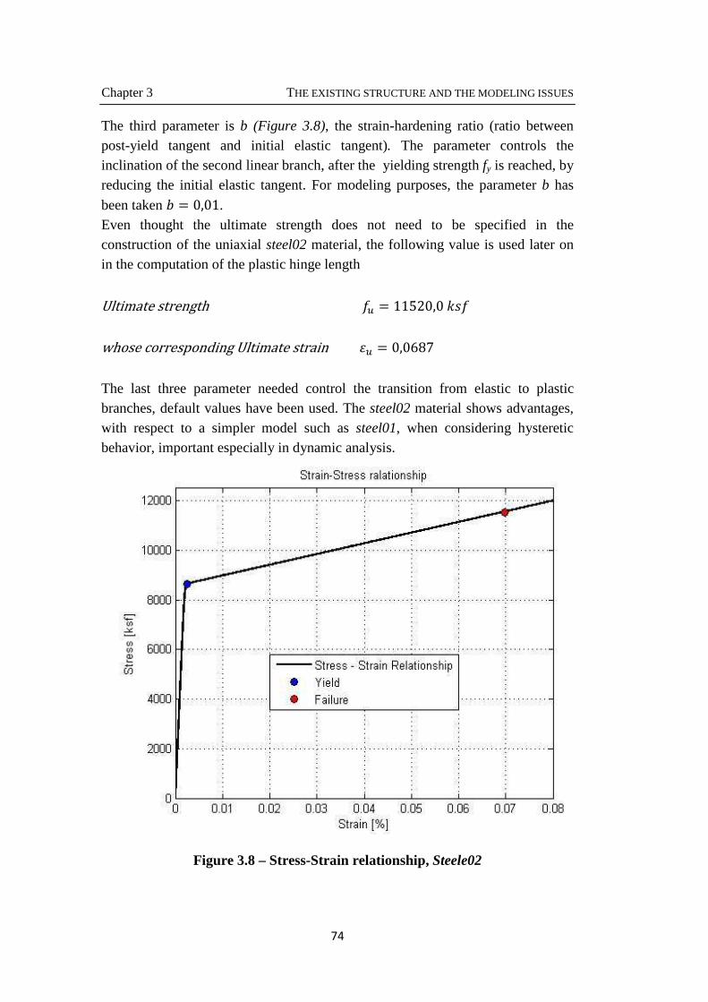
3.3. The prototype materials……………………………………………...66
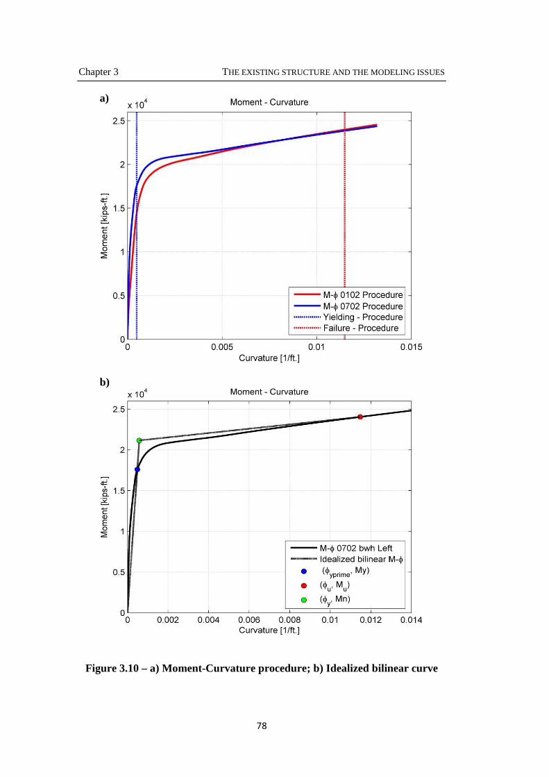
3.3.1. Linear elastic material for the deck……………………..…...66 3.3.2. Elasto-plastic materials for the bents……………….…..…...66 3.3.3. Fiber section definition……………………………..…..…...75 3.3.4. The Moment-Curvature analysis of the section……………..76
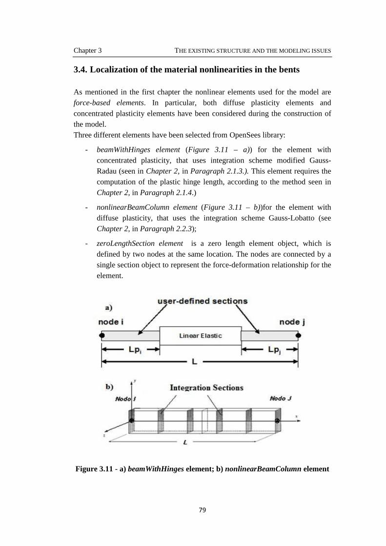
3.4. Localization of the material nonlinearities in the columns………….79
3.4.1. The different scenarios employed in the bents modeling……80
3.5. The Geometrical nonlinearities……………………………………...81
3.6. The Pushover Analysis procedure……………..................................82
3.6.1. The solving algorithms……………........................................82 3.6.2. The integrator ………….…………........................................82 3.6.3. The convergence test……………...........................................83
3.7. The Nonlinear Time History Analysis procedure………….……..…83
3.7.1. The solving algorithms, the integrator and the convergence test…………………………………………………………...83
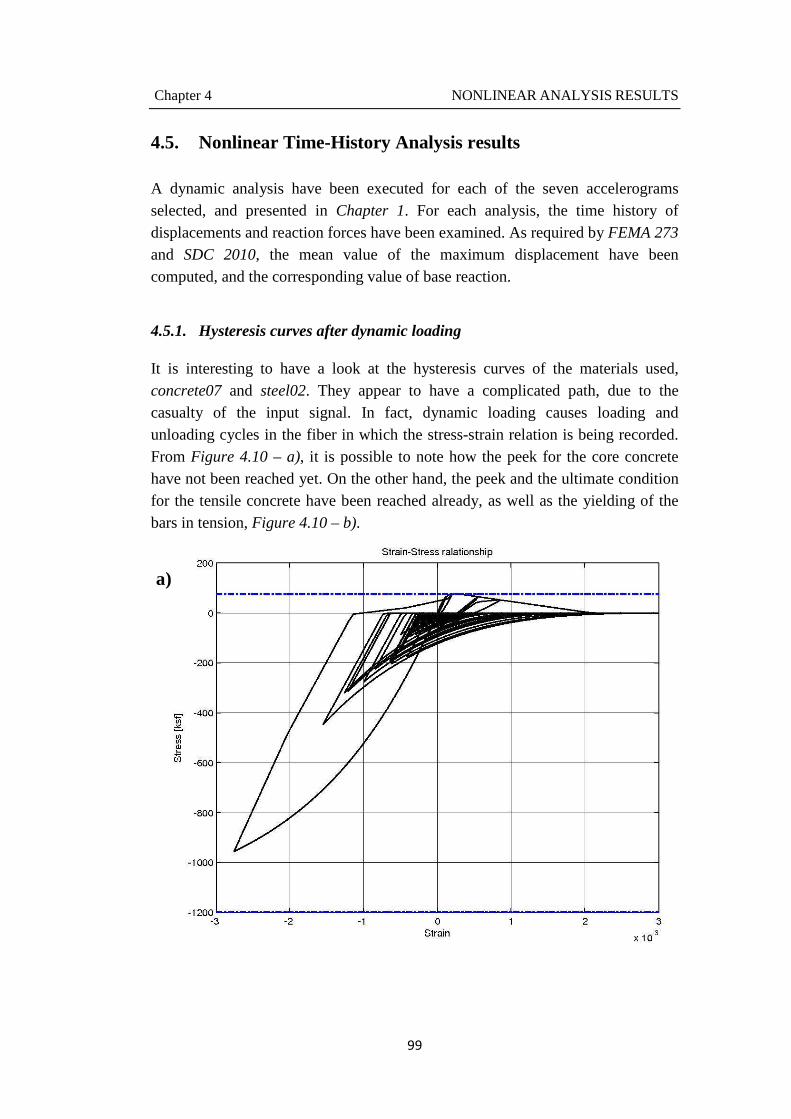
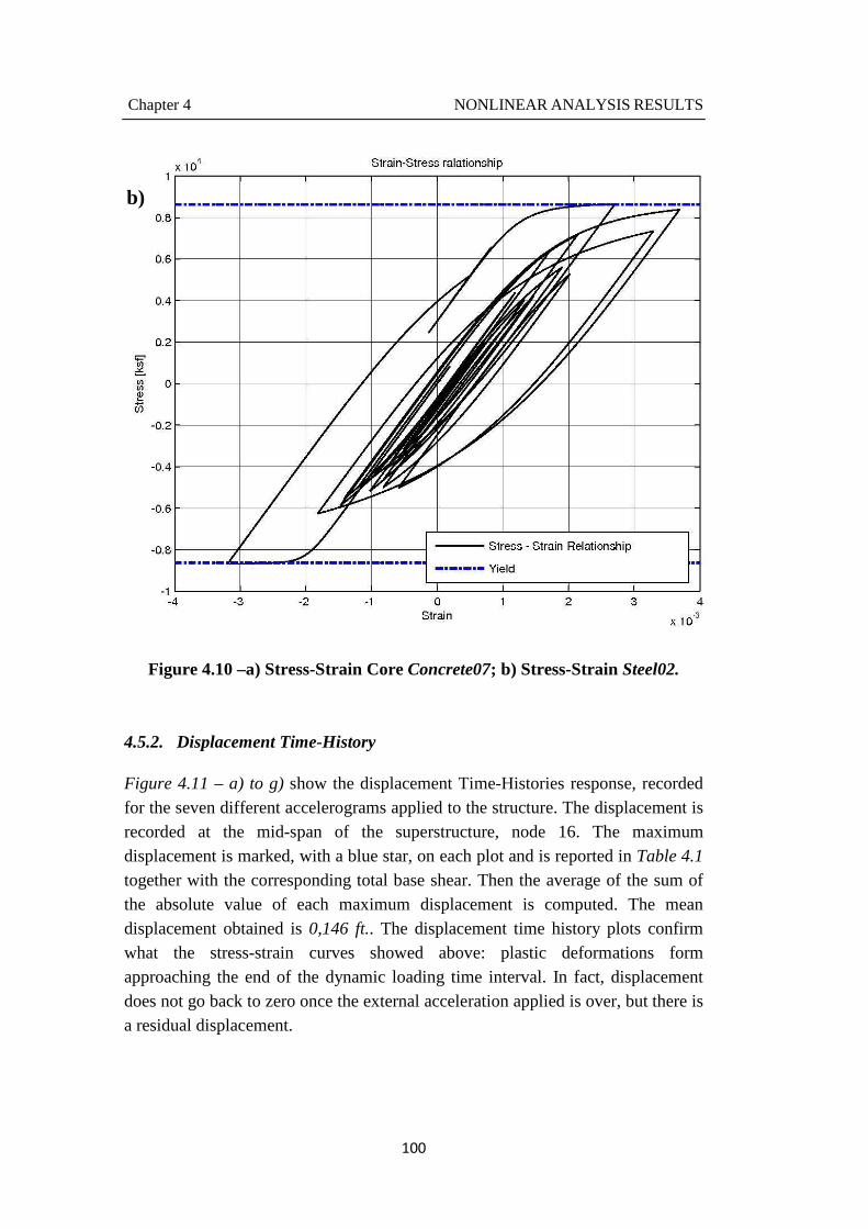
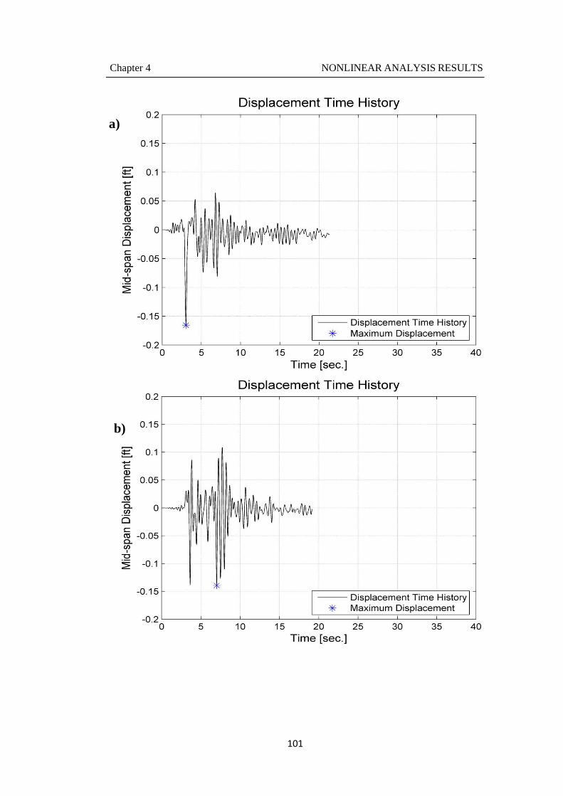
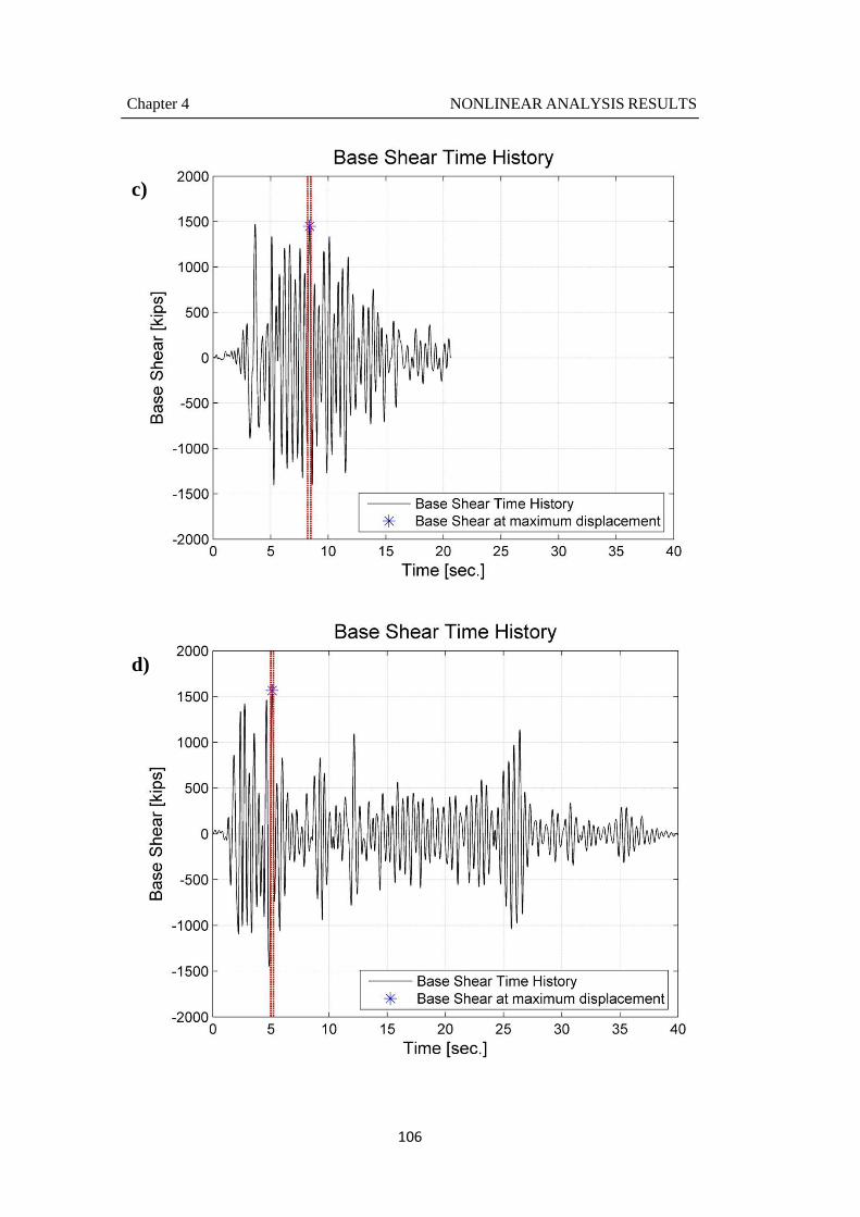
4.5.1. Backbone curves after dynamic loading…………….……….99 4.5.2. Displacement Time-Histories…………..……………..……100 4.5.3. Base shear Time-Histories…………..……………………...104
4.6. Comparison between pushover and time-history results……..……109
INDEX
Conclusion…………………………….………..…………………………....111
List of figures…………………………….…………………………..……...113
List of tables……………………………...………………….………..……..116
References…………………………….………..………………………….....117
INDEX
Introduction
The work for the present thesis started in California, during my semester as an exchange student overseas. California is known worldwide for its seismicity and its effort in the earthquake engineering research field. For this reason, I immediately found interesting the Structural Dynamics Professor, Maria Q. Feng's proposal, to work on a pushover analysis of the existing Jamboree Road Overcrossing bridge. Concrete is a popular building material in California, and for the most part, it serves its functions well. However, concrete is inherently brittle and performs poorly during earthquakes if not reinforced properly. The San Fernando Earthquake of 1971 dramatically demonstrated this characteristic. Shortly thereafter, code writers revised the design provisions for new concrete buildings so to provide adequate ductility to resist strong ground shaking. There remain, nonetheless, millions of square feet of non-ductile concrete buildings in California. The purpose of this work is to perform a Pushover Analysis and compare the results with those of a Nonlinear Time-History Analysis of an existing bridge, located in Southern California. The analyses have been executed through the software OpenSees, the Open System for Earthquake Engineering Simulation. The bridge Jamboree Road Overcrossing is classified as a Standard Ordinary Bridge. In fact, the JRO is a typical three-span continuous cast-in-place pre-stressed post-tension box-girder. The total length of the bridge is 366 ft., and the height of the two bents are respectively 26,41 ft. and 28,41 ft.. Both the Pushover Analysis and the Nonlinear Time-History Analysis require the use of a model that takes into account for the nonlinearities of the system. In fact, in order to execute nonlinear analyses of highway bridges it is essential to
INTRODUCTION
2
incorporate an accurate model of the material behavior. It has been observed that, after the occurrence of destructive earthquakes, one of the most damaged elements on highway bridges is a column. To evaluate the performance of bridge columns during seismic events an adequate model of the column must be incorporated. Part of the work of the present thesis is, in fact, dedicated to the modeling of bents. Different types of nonlinear element have been studied and modeled, with emphasis on the plasticity zone length determination and location. Furthermore, different models for concrete and steel materials have been considered, and the selection of the parameters that define the constitutive laws of the different materials have been accurate. The work is structured into four chapters, to follow a brief overview of the content.
The first chapter introduces the concepts related to capacity design, as the actual philosophy of seismic design. Furthermore, nonlinear analyses both static, pushover, and dynamic, time-history, are presented. The final paragraph concludes with a short description on how to determine the seismic demand at a specific site, according to the latest design criteria in California.
The second chapter deals with the formulation of force-based finite elements and the issues regarding the objectivity of the response in nonlinear field. Both concentrated and distributed plasticity elements are discussed into detail.
The third chapter presents the existing structure, the software used OpenSees, and the modeling assumptions and issues. The creation of the nonlinear model represents a central part in this work. Nonlinear material constitutive laws, for concrete and reinforcing steel, are discussed into detail; as well as the different scenarios employed in the columns modeling.
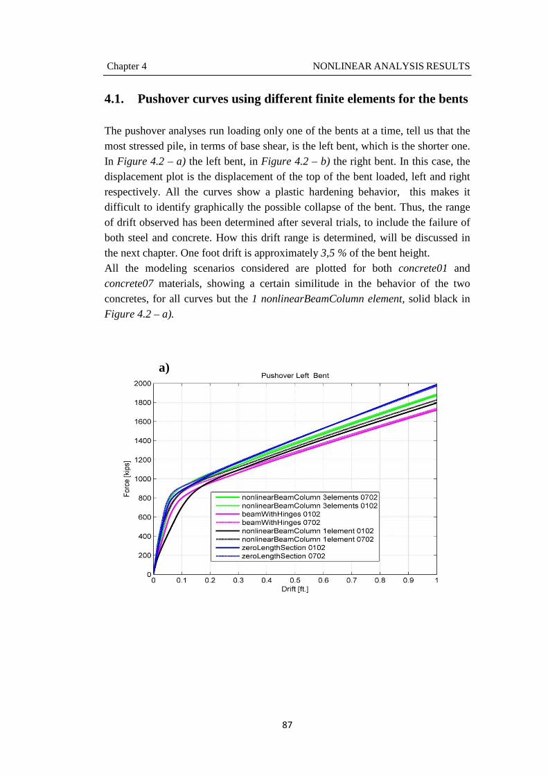
Finally, the results of the pushover analysis are presented in chapter four. Capacity curves are examined for the different model scenarios used, and failure modes of concrete and steel are discussed. Capacity curve is converted into capacity spectrum and intersected with the design spectrum. In the last paragraph, the results of nonlinear time-history analyses are compared to those of pushover analysis.
Chapter 1
NONLINEAR ANALYSIS IN SEISMIC DESIGN OF BRIDGES
The seismic demands on a bridge structure, subject to a particular ground motion, can be estimated through an equivalent analysis of a mathematical model that incorporates the behavior of the superstructure, piers, footing, and soil system. The idealized model should properly represent the actual geometry, boundary conditions, gravity load, mass distribution, energy dissipation, and nonlinear properties of all major components of the bridge. In this way, confident results can be achieved for a variety of earthquake scenarios. A simple linear elastic model of a bridge structure would only accurately capture the static and dynamic behavior of the system when stresses in all elements of the bridge do not exceed their elastic limit. Beyond that demand level, a linear model will fail to represent many sources of inelastic response of the bridge. The forces and displacements generated by a linear elastic analysis will differ considerably from the actual force demands on the structure. Nonlinear modeling and analysis allow more accurate determination of stresses, strains, deformations, forces, and displacements of critical components, results that can then be utilized for the final design of the bridge subsystems or evaluation of the bridge global capacity and ductility. Two categories of nonlinear behavior are incorporated in the bridge model, to properly represent the expected response under moderate to intense levels of seismic demand. The first category consists of inelastic behavior of elements and cross sections due to nonlinear material stress-strain relations, as well as the
Chapter 1 NONLINEAR ANALYSIS IN SEISMIC DESIGN OF BRIDGES
4
presence of gaps, dampers, or nonlinear springs in special bridge components. The precise definition of material and geometric nonlinearities in the model is not an easy task, as the resulting response values are generally highly sensitive to small variations in the input parameters. The second category consists of geometric
nonlinearities that represent second order or P-∆ effects on a structure, where the equilibrium condition is determined under the deformed shape of the structure. The second nonlinearity category is incorporated directly in the analysis algorithm. The additional level of sophistication of the nonlinear model will increase the computational effort required for the analysis, as well as the difficulty in the interpretation of results. Thus, the most important goal to achieve, while building a nonlinear model, is the balance between model complexities and the corresponding gain in accuracy of the results. The Guidelines for Nonlinear
Analysis of Bridge Structures in California [1] suggest for an Ordinary Standard Bridge structure to simplify the model in such way that column plastic hinge zone shall be considered nonlinear, while cap beam and column outside plastic hinge zone shall be considered linear elastic. The JRO can be considered a Standard Ordinary Bridge, due to the simplicity of its geometry. According to Caltrans, Ordinary bridges are not designed to respond elastically during the Maximum Earthquake because of economic constraints and the uncertainties in predicting seismic demands. Thus, the objective is to take advantage of ductility and post elastic strength to meet the established performance criteria with a minimum capital investment. Such philosophy is based on the relatively low probability that a major earthquake will occur at a given site, and the willingness to absorb the repair cost at if ever a major earthquake occurs. In general, the modeling assumptions should be independent of the computer program used to perform the nonlinear static and dynamic analyses; however, mathematical models are often limited by the capabilities of the computer program utilized.
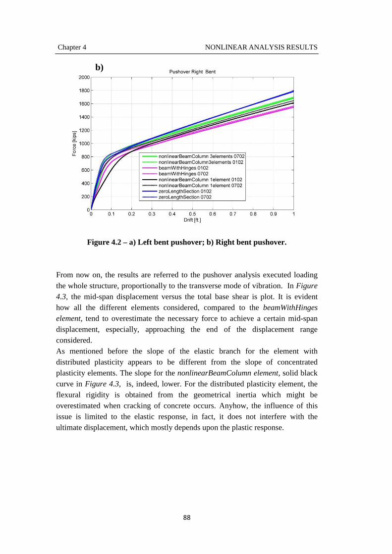
Chapter 1 NONLINEAR ANALYSIS IN SEISMIC DESIGN OF BRIDGES
5
1.1. Seismic design philosophy for bridges: capacity design
Capacity design criteria have been adopted in seismic design, to ensure satisfactory performance during seismic events. Capacity design is a design process where the designer decides which elements of a structural system will be permitted to yield (ductile components) and which elements are to remain elastic (brittle components). Capacity design exploits nonlinear ability of certain predetermined components of the structure; this represents an advantage over designing the whole structure for an elastic response, which would be economically unfeasible. Once ductile and brittle systems are decided upon, design proceeds according to the following guidelines:
- Ductile components are designed with sufficient deformation capacity such that they may satisfy displacement-based demand-capacity ratio;
- Brittle components are designed to achieve sufficient strength levels such that they may satisfy strength-based demand-capacity ratio.
Thus, one can state that the aims of Capacity Design are:
i. ensure that ductile modes of failure (i.e. flexure) should precede brittle modes of failure (i.e. shear) with sufficient reliability, by providing adequate overstrength so that the desired yielding mechanism occurs and non-ductile failure mechanisms (such as concrete crushing, shear cracking, elastic buckling, and fracture) are prevented;
ii. prevent the formation of a soft-story mechanism;
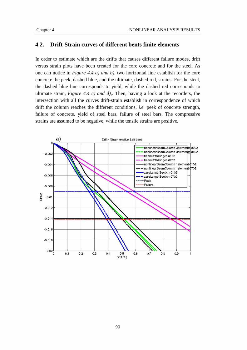
iii. ensure that certain parts of the structure will remain elastic if it is so desired (e.g. foundation, bridge deck, etc.); in fact, the structure should have an adequate capacity to deform beyond its elastic limit without substantial reduction of the overall resistance against horizontal and vertical loads.
In the following paragraphs, the main concepts involved in capacity design are introduced, i.e., performance level, seismic capacity, ductility of members, predetermined locations of damage and redundancy.
Chapter 1 NONLINEAR ANALYSIS IN SEISMIC DESIGN OF BRIDGES
6
1.1.1. Performance level
The definition of the philosophy of Performance Based Seismic Engineering
(PBSE) [2] is to design a structural system able to sustain a predefined level of damage under a predefined level of earthquake intensity. Usually the following steps are set, in order to establish performance level for different limit states:
- define earthquake loadings with various probabilities of occurrence;
- define various acceptable level of damage;
- combine each earthquake loading with an acceptable level of damage.
Figure 1.1 - b) shows different performance level, and the associated damage level, in correspondence of the Earthquake design level, or frequency of ground shaking events. In particular, the collapse limit state is an extreme event and is defined as the condition where any additional deformation will potentially render a bridge incapable of resisting the loads generated by its self-weight. Structural failure or instability in one or more components usually characterizes collapse. All forces (axial, flexure, shear and torsion) and deformations (rotation and displacement) shall be considered when quantifying the collapse limit state. All bridges shall be designed to withstand deformations imposed by the level of ground shaking that has a 5 percent chance of being exceeded in a 50 years period. All structural components shall be designed to provide sufficient strength and/or ductility, with a reasonable amount of reserve capacity, to ensure collapse will be prevented during the Maximum Earthquake, Figure 1.1- b) very rare earthquake, Figure
1.2 – a) collapse in the capacity curve.
1.1.2. Seismic capacity
Seismic capacity is defined as the largest deformation a structure or element can undergo without a significant degradation in its ability to carry loads. For example, during the lateral loading test of reinforced concrete bridge column, the column undergoes larger displacements as the lateral load is increased. However, at a certain point, the seismic capacity of the column is reached and the column can be pushed farther using less force. In Figure 1.1 – a) an example of capacity curve.
Chapter 1 NONLINEAR ANALYSIS IN SEISMIC DESIGN OF BRIDGES
7
Figure 1.1 – a) Capacity curve; b) Performance Objective and Hazard Level Matrix
Chapter 1 NONLINEAR ANALYSIS IN SEISMIC DESIGN OF BRIDGES
8
1.1.3. Ductility and predetermined locations of damage
Ductility is the ratio of ultimate deformation to the deformation at yield.
(1.1) � = ������������
A ductile structural member responds with inelastic deformation to cyclic loading without significant degradation of strength or stiffness. The most desirable type of ductile response in bridge systems, during hysteric force-deformation cycles, is energy dissipation. There are two ways to obtain energy dissipation:
- internally, within the structural members, by the formation of flexural plastic hinges;
- externally, with isolation bearings or external dampers.
The deformations for ductile structural components are limited so the structure will not exceed its inelastic deformation capacity. It is not desirable that concrete superstructure of a bridge undergo significant inelastic deformations, because of the potential to jeopardize public safety. Furthermore, superstructure damage in continuous bridges is difficult to repair to a serviceable condition. Thus, inelastic behavior shall be limited to predetermined locations within the bridge locations that can be easily inspected and repaired following an earthquake. Preferably, inelastic behavior on most bridges shall be located in columns, pier walls, backwalls, wingwalls, seismic isolation and damping devices, bearings, shear keys and steel end diaphragms. In order to prevent collapse of the structure, redundancy should also be applied to bridges whenever possible. An alternative load path should be provided. For example, in bridge systems like single column bents, redundancy can be improved by establishing a greater margin between the component’s dependable capacity and its expected response to seismic action, continuity at expansion joints with reliable shear keys and restrainers, and load transfer to the abutments.
Chapter 1 NONLINEAR ANALYSIS IN SEISMIC DESIGN OF BRIDGES
9
1.2. Types of nonlinear analyses
The aim of a nonlinear analysis is to obtain a representation of the structure's ability to resist the seismic demand. Nonlinear analyses are divided into two categories:
i. Static, i.e. Pushover analysis;
ii. Dynamic, i.e. Time-History analysis.
To follow the two analyses are briefly introduced, with particular reference to bridge analysis.
1.2.1. Nonlinear Static Analysis: Pushover
A Pushover analysis is a static, nonlinear procedure in which the magnitude of the applied load is incrementally increased following a predefined reference load pattern. By increasing the magnitude of the loading, it is possible to investigate weak links and failure modes of the bridge structure. The goal of the static pushover analysis is to evaluate the overall strength, typically measured through base shear Vb, yield, and maximum displacement δy and δu, and thus, the ductility capacity µc of the bridge structure. The pushover analysis of a bridge is conducted as a displacement controlled
method to a specified limiting displacement value to capture the softening behavior of the structure by monitoring the displacement at a point of reference, such as one of the column’s top nodes or the center of the superstructure span. A displacement control strategy requires the specification of an incremental displacement that have to occur at a nodal d.o.f.. The strategy then iterates to determine what load factor, α, is required to impose that incremental displacement. The base shear Vb is proportional to such load factor α, and a global force-displacement capacity curve can be plot, see Figure 1.2. The load patterns used for bridges analyses are either uniform, or inverse triangles, applied to the columns, or proportional to the first significant vibration mode in the direction considered. To interpret the results of pushover analyses the Capacity Spectrum Method (CSM)
might be used. The CSM uses the intersection of the global force-displacement capacity curve and the response spectrum, representation of the earthquake demand, to estimate the maximum displacement demand on the structure, or performance point. The CSM is a very useful tool in the evaluation and retrofit design of existing concrete buildings, because the graphical representation
Chapter 1 NONLINEAR ANALYSIS IN SEISMIC DESIGN OF BRIDGES
10
provides a clear picture of how a building responds to earthquake ground motion. Thus, the CSM consists of the following main steps:
i. evaluation of the global force-displacement capacity curve. For bridges the curve is in terms of base-shear and mid-span displacement, see Figure
1.1 – a);
ii. conversion of the capacity curve into a capacity spectrum;
iii. determination of the demand spectrum;
iv. determination of the performance point of the structure.
Figure 1.2 – Capacity curve of a frame structure
From the capacity curve to the capacity spectrum (ATC 40) [3]
In order to use the CSM to determine the performance point, it is necessary to convert the capacity curve, or pushover curve, to a capacity spectrum. The pushover curve is in terms of base shear and roof displacement, in the specific case of bridges mid-span displacement, while the capacity spectrum is in the format Acceleration-Displacement Response Spectra (ADRS). The spectral acceleration is indicated later on as Sa, the spectral displacement is Sd. The following equations are needed in order to transform the pushover curve into a capacity spectrum
Chapter 1 NONLINEAR ANALYSIS IN SEISMIC DESIGN OF BRIDGES
11
(1.2) ��� = ∑ ������
���� ∑ (�����)�
�����
(1.3) �� = �∑ ������
���� ��
�∑ ���
���� ��∑ (�����)��
����
(1.4) !" = #$ /��
(1.5) !& = �'(()*+�,'((),�
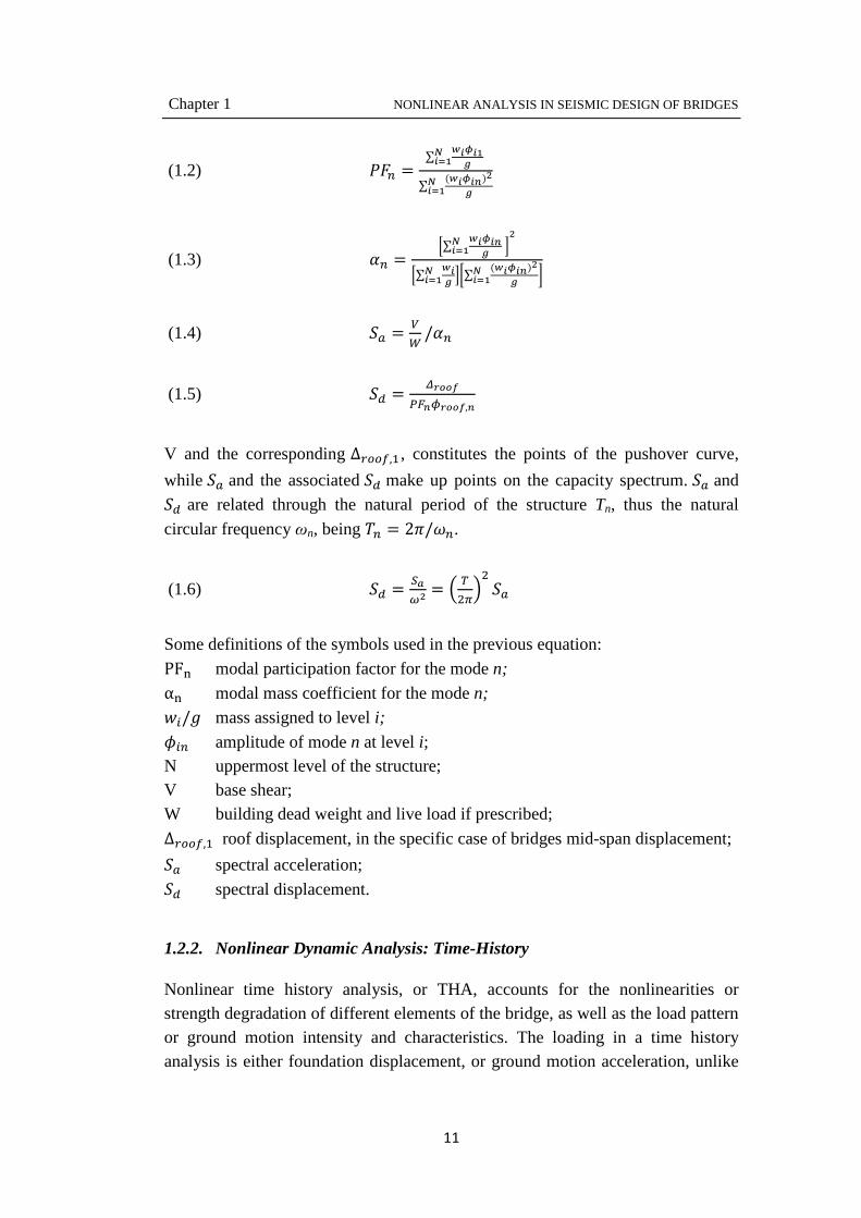
V and the corresponding Δ/001,2, constitutes the points of the pushover curve,
while !" and the associated !& make up points on the capacity spectrum. !" and
!& are related through the natural period of the structure Tn, thus the natural
circular frequency ωn, being 3� = 25/6�.
(1.6) !& = 78� = 9 :
;<=; !"
Some definitions of the symbols used in the previous equation:
PF@ modal participation factor for the mode n;
α@ modal mass coefficient for the mode n;
BC/D mass assigned to level i;
EC� amplitude of mode n at level i; N uppermost level of the structure; V base shear; W building dead weight and live load if prescribed;
Δ/001,2 roof displacement, in the specific case of bridges mid-span displacement;
!" spectral acceleration;
!& spectral displacement.
1.2.2. Nonlinear Dynamic Analysis: Time-History
Nonlinear time history analysis, or THA, accounts for the nonlinearities or strength degradation of different elements of the bridge, as well as the load pattern or ground motion intensity and characteristics. The loading in a time history analysis is either foundation displacement, or ground motion acceleration, unlike
Chapter 1 NONLINEAR ANALYSIS IN SEISMIC DESIGN OF BRIDGES
12
for the pushover analysis where loads are externally applied at the joints or members of the structure. The design displacements are not established using a target displacement, but instead are determined directly through dynamic analysis using suites of ground motion records. Inertial forces are produced in the structure when the structure suddenly deforms due to ground motion and internal forces are produced in the structural members. The main disadvantage of the time history analysis method is the high computational and analytical effort required and the large amount of output information produced. During the analysis, the capacity of the main bridge components is evaluated as a function of time, based on the nonlinear behavior determined for the elements and materials. This evaluation is carried out for several input ground motions, seven according to FEMA 273 [4], and the response of the structure is recorded at every time step. However, the evaluation of the capacity using the THA method at each time step produces superior results, since it allows for redistribution of internal forces within the structure. In general, solution of the dynamic response of structural systems is the direct numerical integration of the dynamic equilibrium equations at a discrete point in time. This analysis is initiated at the undisturbed static condition of the structure and repeated for the duration of the ground motion input with equal time increments to obtain the complete structural response time history under a specific excitation. The step-by-step solution methods attempt to satisfy dynamic equilibrium at discrete time steps and may require iteration, especially when nonlinear behavior is developed in the structure and the stiffness of the complete structural system must be recalculated due to degradation of strength and redistribution of forces. Different numerical techniques have been studied by numerous researchers and are generally classified as either explicit or implicit integration methods.
Chapter 1 NONLINEAR ANALYSIS IN SEISMIC DESIGN OF BRIDGES
13
1.3. The seismic demand
The displacement ductility approach, frequently used nowadays in seismic design, requires the designer to ensure that the structural system and its individual components have enough deformation capacity to withstand the displacements imposed by the Maximum Earthquake. In order to quantify how large the displacement imposed by the Maximum Earthquake is, the seismic demand corresponding to the particular site considered must be determined.
Three levels of earthquake hazard are used to define ground shaking:
- Serviceability Earthquake, defined probabilistically as the level of ground shaking that has a 50 percent chance of being exceeded in a 50 years period;
- Design Earthquake, defined probabilistically as the level of ground shaking that has a 10 percent chance of being exceeded in a 50 years period;
- Maximum Earthquake, defined deterministically as the maximum level of earthquake ground motion which may ever be expected at the building site within the known geologic framework. Corresponds to a level of ground shaking that has a 5 percent chance of being exceeded in a 50 years period.
1.3.2. Development of the design spectrum (SDC 2010, Annex B) [5]
The demand spectrum, or elastic design response spectrum 5% damped, is developed according to Caltrans Seismic Design Criteria 2010 (SDC), Version
1.6, Annex B [5], that specify the minimum seismic requirements for Standard Ordinary Bridges. The elastic design response spectrum 5% damped, also called the design seismic hazard, represents the seismic demand at a specific site. When the design seismic hazard occurs, Ordinary bridges that meets SDC requirements are expected to remain standing but may suffer significant damage requiring closure. The design seismic hazard is based on the envelope of a deterministic spectrum and a probabilistic spectrum. The envelope of the spectra, used for design, is defined as the greater of:
Chapter 1 NONLINEAR ANALYSIS IN SEISMIC DESIGN OF BRIDGES
14
- a probabilistic spectrum based on a 5% in 50 years probability of exceedance (or 975-year return period);
- a deterministic spectrum based on the largest median response resulting from the maximum rupture (corresponding to Mmax) of any fault in the vicinity of the bridge site;
- a statewide minimum spectrum defined as the median spectrum generated by a magnitude 6.5 earthquake on a strike-slip fault located 12 kilometers from the bridge site.
The deterministic spectrum
The deterministic spectrum is calculated as the arithmetic average of median response spectra calculated using the Campbell-Bozorgnia (2008) and Chiou-
Youngs (2008) ground motion prediction equations (GMPE’s), developed under the Next Generation Attenuation project coordinated through the PEER-Lifelines
program. The ground motion prediction equations are applied to all faults in or near California considered to be active in the last 700,000 years (late quaternary age) and capable of producing a moment magnitude earthquake of 6.0 or greater. In application of these ground motion prediction equations, the earthquake magnitude should be set to the maximum moment magnitude, as recommended by California Geological Survey (1997, 2005). The minimum spectrum is defined as the average of the median predictions of Campbell-Bozorgnia (2008) and Chiou-Youngs (2008) for a scenario M=6.5 vertical strike-slip event occurring at a distance of 12 km (7.5 miles). While this scenario establishes the minimum spectrum, the spectrum is intended to represent the possibility of a wide range of magnitude-distance scenarios.
The probabilistic spectrum
The probabilistic spectrum is obtained from the USGS Seismic Hazard Map
(Petersen, 2008) for the 5% in 50 years probability of exceedance (or 975 year return period). Since the USGS Seismic Hazard Map spectral values are published only for VS30 =
760 m/s, soil amplification factors must be applied for other site conditions. The site amplification factors shall be based on an average of those derived from the Boore-Atkinson (2008), Campbell-Bozorgnia (2008), and Chiou-Youngs (2008)
Chapter 1 NONLINEAR ANALYSIS IN SEISMIC DESIGN OF BRIDGES
15
ground motion prediction models (the same models used for the development of the USGS map).
The demand spectrum
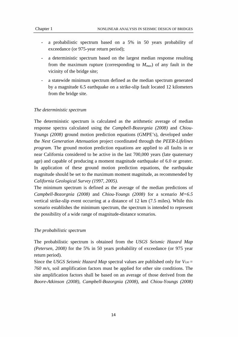
The Demand Spectrum has been obtained from the Caltrans ARS Online (v1.0.4) [6]. Only three input parameters are needed: the geographical coordinates, latitude and longitude, and the VS30, the average shear wave velocity in the upper 30 meters of the soil profile. Spectrum adjustment factors are incorporated in the selection of the demand spectrum. In fact, the design spectrum may need to be modified to account for seismological effects related to being in close proximity to a rupturing fault and/or placement on top of a deep sedimentary basin, see Figure 1.3 for faults location. The average shear wave velocity, VS30, has been obtained from USGS maps [7], see Figure 1.4, and the value considered is 300 m/s. Once available the average shear wave velocity, and the geographical coordinates, the online tool computes the different spectra, as described previously in the paragraph. The calculated spectra are shown in Figure 1.5 – a), while the envelope is shown in Figure 1.5 – b).
Figure 1.3 – Faults location near site.
Chapter 1 NONLINEAR ANALYSIS IN SEISMIC DESIGN OF BRIDGES
16
Figure 1.4 – USGS VS30 maps, Western U.S.
Chapter 1 NONLINEAR ANALYSIS IN SEISMIC DESIGN OF BRIDGES
17
Figure 1.5 – a) Calculated spectra; b) Design Envelope.
a)
b)
Chapter 1 NONLINEAR ANALYSIS IN SEISMIC DESIGN OF BRIDGES
18
1.3.3. Acceleration time history (FEMA 273) [4]
According to FEMA 273, Time-History Analysis shall be performed with no fewer than three data sets of appropriate ground motion time histories that shall be selected and scaled from no fewer than three recorded events. Appropriate time histories shall have magnitude, fault distances, and source mechanisms that are consistent with those that control the design earthquake ground motion. Furthermore, FEMA 273 specify the two following criteria for the selection of ground motion:
- a minimum of three pairs of ground motion records are used in the analysis, where each ground motion corresponds to the hazard level appropriate to the desired performance objective and consists of two orthogonal components of the record. The envelope of the three records is used to compute the maximum response of the bridge;
- seven different ground motions, thus, the median value of response obtained from the different records is used to estimate the peak response of the bridge.
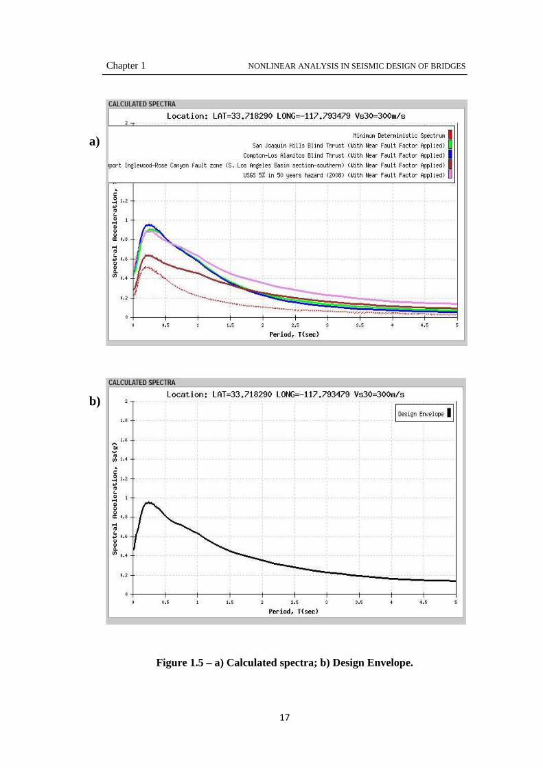
Firstly a deaggregation, using USGS interactive tool [8], have been carried out, in order to establish which ground shaking parameters, i.e. the magnitude interval and distances from the site, have the most influence on the site considered. The input parameters are the geographical coordinates and the shear wave velocity Vs30. Figure 1.6 – a) shows the histogram with the results of the deaggregation that have been used as input parameters in the MATLAB® [9] code employed to select the seven accelerograms. According to FEMA 273, the data sets shall be scaled such that the average value of the SRSS spectra does not fall below 1,4 times the 5% damped spectrum for the design earthquake for periods between 0.2T seconds and 1.5T seconds (where T is the fundamental period of the building). Figure 1.6 - b) shows the magnitude function of the distance of the ground shaking from the site considered. Each dot is an accelerometer present in the Next Generation Attenuation Relationships for
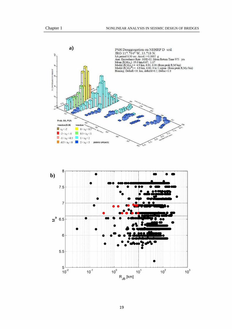
Western U.S. database; the red dots fall in the input interval magnitude defined by the user. Figure 1.6 - c) shows the interval, dashed lines, in which the MATLAB® code looks for the most correspondence between the input 5%
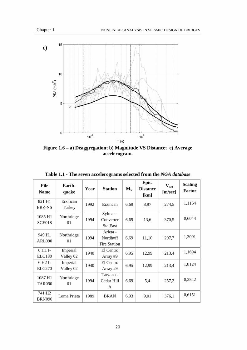
damped elastic response spectra and the spectra selected, using the selection parameters. Figure 1.6 - c) also shows the average accelerograms, which is close to the 5% damped spectrum. The seven accelerograms selected from the NGA database [10] are described in Table 1.1 and shown in Figure 1.7 a) to g).
Chapter 1 NONLINEAR ANALYSIS IN SEISMIC DESIGN OF BRIDGES
19
a)
b)
Chapter 1 NONLINEAR ANALYSIS IN SEISMIC DESIGN OF BRIDGES
20
Figure 1.6 – a) Deaggregation; b) Magnitude VS Distance; c) Average
accelerogram.
Table 1.1 - The seven accelerograms selected from the NGA database
File Name
Earth-quake
Year Station Mw Epic.
Distance [km]
Vs30
[m/sec]
Scaling Factor
821 H1 ERZ-NS
Erzincan Turkey
1992 Erzincan 6,69 8,97 274,5 1,1164
1085 H1 SCE018
Northridge 01
1994 Sylmar - Converter Sta East
6,69 13,6 370,5 0,6044
949 H1 ARL090
Northridge 01
1994 Arleta -
Nordhoff Fire Station
6,69 11,10 297,7 1,3001
6 H1 I-ELC180
Imperial Valley 02
1940 El Centro Array #9
6,95 12,99 213,4 1,1694
6 H2 I-ELC270
Imperial Valley 02
1940 El Centro Array #9
6,95 12,99 213,4 1,8124
1087 H1 TAR090
Northridge 01
1994 Tarzana - Cedar Hill
A 6,69 5,4 257,2 0,2542
741 H2 BRN090
Loma Prieta 1989 BRAN 6,93 9,01 376,1 0,6151
c)
Chapter 1 NONLINEAR ANALYSIS IN SEISMIC DESIGN OF BRIDGES
21
a)
b)
Chapter 1 NONLINEAR ANALYSIS IN SEISMIC DESIGN OF BRIDGES
22
c)
d)
Chapter 1 NONLINEAR ANALYSIS IN SEISMIC DESIGN OF BRIDGES
23
e)
f)
Chapter 1 NONLINEAR ANALYSIS IN SEISMIC DESIGN OF BRIDGES
24
Figure 1.7 – Accelerograms a) 821 H1 ERZ-NS; b) 1085 H1 SCE018;
Based on the complexity of the model it is possible to define a classification of modeling strategies. One can distinguish the following model categories with increasing level of refinement and complexity:
i. Global models: the non-linear response of a structure is represented at select degrees of freedom;
ii. Discrete finite element (member) models: in this case the structure is modeled as an assembly of interconnected frame elements with either lumped or distributed nonlinearities;
iii. Microscopic finite element models: the members and joints of the structure are discretised into several large or small two or three-dimensional finite elements.
While such refined finite element models might be suitable for the detailed study of small parts of the structure, such as beam to column joints, frame models are presently the only economical solution for the nonlinear dynamic response analysis of structures with several hundred members. Member finite element models are the best compromise between simplicity and accuracy in non-linear
Chapter 2 FINITE ELEMENT MODELS FOR THE NONLINEAR MATERIAL RESPONSE OF BEAM
COLUMN ELEMENTS: FORMULATIONS AND OBJECTIVITY OF THE RESPONSE
26
seismic response studies and represent the simplest class of model that still allows significant insight into the seismic response of members and of the entire structure. Modeling of material nonlinearities in frame analysis can be classified into two main categories:
i. lumped, or concentrated, plasticity approach is characterized by inserting discrete nonlinear moment-rotation hinges at the ends of otherwise linear elements. This approach provides an efficient means of modeling and controlling plastic hinge formation. Clearly one of the main concerns for this type of element is the determination of the plastic hinge length, which will be discussed in more detail later.
ii. distributed plasticity models provide a more general framework for nonlinear frame analysis, where nonlinearities can develop anywhere along the member. This kind of element is based on a fiber approach, to represent the cross section behavior, where each fiber is associated with an uniaxial stress-strain relationship.
After the selection of the element type, another main step is the selection of one of the two methods available for the implementation of the formulation:
i. displacement-based formulations, in which the displacement fields along the element are expressed as functions of the nodal displacements. The assumed displacement fields are approximations of the actual displacement fields; thus, several elements per member are used to obtain a good approximation of the exact response.
ii. force-based formulations, or flexibility-based formulations, in which the internal force fields are expressed as functions of the nodal forces. Force-based elements are particularly suited for non- linear frame analysis because they are exact within the framework of the classical beam theories (Spacone et al. 1996 a, b). Because of the precision of force-based elements, it is possible to use just one element per structural member, leading to considerable savings in the total number of degrees of freedom in the structural model.
In a displacement-based approach, the displacement field is imposed, whereas in a force-based element equilibrium is strictly satisfied and no restraints are placed on the development of inelastic deformations throughout the member. For this reason, force-based formulations are extremely appealing for earthquake engineering applications, where significant material nonlinearities are expected to occur.
Chapter 2 FINITE ELEMENT MODELS FOR THE NONLINEAR MATERIAL RESPONSE OF BEAM
COLUMN ELEMENTS: FORMULATIONS AND OBJECTIVITY OF THE RESPONSE
27
For a hardening type of sectional behavior, both force-based and displacement-based elements produce an objective response at the global (force-displacement) and local (moment-curvature) levels, whereas the results are non-objective in the case of a softening sectional law. This numerical issue, commonly known as localization, was firstly discussed by Zeris and Mahin, 1988 [11] for displacement-based elements, and Coleman and Spacone, 2001- a) [12] studied it for force-based elements. To follow the force-based formulation will be discussed in more detail, both for concentrated plasticity models and distributed plasticity models.
Chapter 2 FINITE ELEMENT MODELS FOR THE NONLINEAR MATERIAL RESPONSE OF BEAM
COLUMN ELEMENTS: FORMULATIONS AND OBJECTIVITY OF THE RESPONSE
Historically, concentrated plasticity models were the first formulations implemented in structural analysis softwares for earthquake engineering simulations purposes, developed to include nonlinearities into beam-column elements. Their first appearance dates back to the 1960s. In this models all the elements of the structure acts as linear elastic, while the concentration of the plasticity is into rotational springs, or plastic hinges. The fact that all the structure is modeled as linear elastic, and only localized nonlinearities are introduced, represents the largest advantage. It reduces the computational effort and the complexity of the model. On the other hand, concentrated plasticity models are based on several assumptions, increasing the risk of inaccuracy, or inadequacy, of the analysis output. Thus, the need of great experience to overcome the following main issues:
- distribution of the concentrated nonlinearities into the structure, in fact plastic hinges location cannot be known for sure a priori;
- evaluation of the length of such plastic hinges; many formulas are proposed in literature, all of them require the assumption that plastic hinges will form at a specific location;
- selection of the appropriate stress-strain relationship attributed to the nonlinear zones.
2.1.1. Element Formulation (Scott et al. 1996) [13]
Force-based beam-column elements are formulated in a basic system without rigid-body displacement modes. The vector v contains the element deformations, assumed to be small compared to the element length. For a simply supported beam it is possible to define three element deformations, for two-dimensional
elements, and six for three-dimensional elements (see Figure 2.1); � = � (�) is a function of the element deformations. It represents the vector of forces in the basic system. The section behavior is expressed in terms of the section deformations, e,
and � = � (�) represents the corresponding section forces. Equilibrium between the basic forces and section forces is expressed in strong form as
(2.1) � = �
where the matrix b contains interpolation functions relating section forces to basic forces from equilibrium of the basic system.
Chapter 2 FINITE ELEMENT MODELS FOR THE NONLINEAR MATERIAL RESPONSE OF BEAM
COLUMN ELEMENTS: FORMULATIONS AND OBJECTIVITY OF THE RESPONSE
29
Figure 2.1 - Basic simply supported element and section
The axial force and bending moment at location x along the element for a two-dimensional simply supported basic system is given by the following equilibrium interpolation matrix
(2.2) = 1 0 00 /� − 1 /� � The compatibility relationship between the section and element deformations can be derived from the principle of virtual forces
(2.3) � = � ��� ��
whose linearization with respect to the basic forces gives the section flexibility matrix
(2.4) � = ���� = � ���� ��
The section stiffness matrix is�� = ��/�� . Flexibility matrix �� = ����, is obtained inverting the section stiffness matrix. The element stiffness matrix, k, in
the basic system is the inverse of the element flexibility matrix, � = ���. The compatibility relationship in Eq. 2.3 is evaluated by numerical quadrature
Chapter 2 FINITE ELEMENT MODELS FOR THE NONLINEAR MATERIAL RESPONSE OF BEAM
COLUMN ELEMENTS: FORMULATIONS AND OBJECTIVITY OF THE RESPONSE
30
(2.5) � = ∑ ( ��!"#$%)&%'(%#�
where ) and * are the locations and associated weights, respectively, of the Np
integration points over the element length [0, L]. In a similar manner, the element flexibility matrix is evaluated numerically
(2.6) � = ∑ ( ���!"#$%)&%'(%#�
In force-based elements the bending moments are largest at the element ends, in the absence of member load; therefore it is suitable to use Gauss-Lobatto quadrature. In fact, this technique places integration points at the elements ends. In Figure 2.2 a graphical representation of the four-point Gauss–Lobatto
quadrature rule, where the integrand, bTe, is evaluated at the i-th location )+ and
treated as constant over the length *+. The highest order polynomial integrated
exactly by the Gauss–Lobatto quadrature rule is 2-. − 3, which is two orders lower than Gauss–Legendre quadrature. For a linear-elastic, prismatic beam–column element without member loads, quadratic polynomials appear in the integrand of Eq. 2.3 due to the product of the linear curvature distribution in the vector e with the linear interpolation functions for the bending moment in the matrix b. Therefore, at least three Gauss–Lobatto integration points are required to represent exactly a linear curvature distribution along the element. To represent accurately the nonlinear material response of a force-based beam–column element, four to six Gauss–Lobatto integration points are typically used (Neuenhofer and
Filippou, 1997 [38]).
Figure 2.2 - Application of four-point Gauss–Lobatto quadrature rule to evaluate force-based element compatibility relationship
Chapter 2 FINITE ELEMENT MODELS FOR THE NONLINEAR MATERIAL RESPONSE OF BEAM
COLUMN ELEMENTS: FORMULATIONS AND OBJECTIVITY OF THE RESPONSE
31
2.1.2. Loss of objectivity in force-based beam-column elements
Gauss–Lobatto integration rule permits the spread of plasticity along the element length, which is a primary advantage. For hardening section behavior, the computed element response will converge to a unique solution as the number of integration points increases, while for softening section behavior where deformations localize at a single integration point, a unique solution does not exist and the computed response depends on the characteristic length implied by the integration weights of the Gauss–Lobatto quadrature rule. The lack of uniqueness for the solution, in the case of softening section behavior, leads to a loss of objectivity, where the element response will change as a function of Np. To address the loss of objectivity in force-based beam–column elements, Coleman
and Spacone, 2001 developed a regularization technique that modifies the material stress–strain behavior to maintain a constant energy release after strain-softening initiates. Coleman and Spacone applied this method to the Kent–Park concrete model (Kent and Park 1971 [14]) shown in Figure 2.3, where the shaded area is equal to the energy released after the onset of strain softening
(2.7) 01234 = 0,6678 9:;< − :8 + <,>?@2A2 B
The parameters for the Kent–Park concrete model are: 6 ′8 concrete compressive strength; :8 peak compressive strain; Ec elastic modulus; :;< strain corresponding to 20% of the compressive strength; C?8, concrete fracture energy in compression;
lp plastic hinge length, which acts as the characteristic length for the purpose of providing objective response. As discussed in the previous section, the plastic hinge length in the model is directly related to the element integration rule for force-based elements. For the lp
implied by the number of Gauss–Lobatto integration points, :;< must be modified in order to maintain a constant energy release
(2.8) :;< = 012<,D?@234 − <,>?@2A2 + :8
Chapter 2 FINITE ELEMENT MODELS FOR THE NONLINEAR MATERIAL RESPONSE OF BEAM
COLUMN ELEMENTS: FORMULATIONS AND OBJECTIVITY OF THE RESPONSE
32
Figure 2.3 - Kent–Park concrete stress–strain model with fracture energy
Although this approach maintains objective response at the global level, it affects the local section response through an unnatural coupling of the concrete material properties to the element integration rule. A second regularization is required to correct for the loss of objectivity in the section response, that results from this approach (Coleman and Spacone, 2001 [12]). For the plastic hinge integration
methods presented to follow, EF is specified as part of the element integration rule
and it becomes a free parameter. Therefore, it is possible to determine a plastic hinge length that will maintain a constant energy release without modification to the concrete stress-strain relationship, alleviating the need for a subsequent regularization of the section response. A logical separation of the material properties from the element integration rule is achieved by introducing a plastic hinge length to the element integration rule The determination of the plastic hinge length will be discussed later in the chapter, with reference to the particular method used for the computation of the length needed for the FEM model of the structure, in accordance with the requirements imposed by Caltrans Seismic Design Criteria 2010.
Chapter 2 FINITE ELEMENT MODELS FOR THE NONLINEAR MATERIAL RESPONSE OF BEAM
COLUMN ELEMENTS: FORMULATIONS AND OBJECTIVITY OF THE RESPONSE
33
2.1.3. Plastic hinge integration methods
Now the aim is to achieve objectivity for softening response. The plastic hinge integration methods presented herein are based on the assumption that nonlinear constitutive behavior is confined to regions of length lpI and lpJ at the element ends. As such, the elements are useful for columns or beams that carry small member loads. To represent plastic hinges in force-based beam–column elements, the compatibility relationship is separated into three integrals, one for each hinge region, where plasticity develops, and one for the interior region of the element, which remains linear elastic
The section deformations are integrated numerically over the plastic hinge regions, whereas the contribution of the element interior is assumed to be linear elastic, as mentioned above, and evaluated by the flexibility of the interior region
(2.10) � = ∑ K ��!"#$%L&% + �%MN� �'(%#�
The flexibility matrix of the element interior region, �+OPQ , is evaluated by the
closed-form integral
(2.11) �%MN� = � ����� GHI �
The matrix �RQ contains the elastic flexibility coefficients at a cross section of the interior, assuming the coordinate axis is located at the centroid of the section, with the elastic modulus E, the cross-sectional area A, and the second moment of the cross-sectional area I.
(2.12) ��� = S TAU 00 TAV
W
The linearization of Eq. 2.10 with respect to the basic forces gives the element flexibility as the sum of numerical integration over the plastic hinge regions and the flexibility of the element interior
(2.13) � = ∑ ( ���!"#$%)&%'(%#� + �%MN�
Chapter 2 FINITE ELEMENT MODELS FOR THE NONLINEAR MATERIAL RESPONSE OF BEAM
COLUMN ELEMENTS: FORMULATIONS AND OBJECTIVITY OF THE RESPONSE
34
To represent strain softening in the plastic hinge regions of the element, it is desirable to use a plastic hinge integration rule for Eqs. 2.10 and 2.13 that satisfies the following criteria:
i. sample section forces at the element ends where the bending moments are largest in the absence of member loads;
ii. integrate quadratic polynomials exactly to provide the exact solution for linear curvature distributions;
iii. integrate deformations over the specified lengths lpI and lpJ using a single section in each plastic hinge region.
The Gauss–Lobatto integration rule for distributed plasticity satisfies the first two criteria, but it does not satisfy the third because the plastic hinge lengths are implied by the number of integration points, Np.
The midpoint integration rule
The most accurate one-point integration method is the midpoint rule, for which
the integration points are located at the center of each plastic hinge region,) =[EYZ/2, � − EY[/2] , and the weights are equal to the plastic hinge lengths, * =[EYZ , EY[]. The midpoint rule is illustrated in Figure 2.4- a). The integration points are not located at the element ends where the maximum bending moments occur in the absence of member loads, and this represents the major disadvantage of the midpoint integration rule. As a result, the element will exhibit a larger flexural capacity than expected, which in fact will be a function of the plastic hinge lengths. Furthermore, the midpoint rule gives the exact integration of only linear functions, thus, there is an error in the integration of quadratic polynomials. In light of the above considerations, the midpoint plastic hinge integration method satisfies criterion three but not one or two.
The endpoint integration rule
Another one-point integration rule locates the integration points at the element
ends, ) = [0, �], while the integration weights remain equal to the plastic hinge
lengths, * = [EYZ , EY[], as shown in Figure 2.4 – b). However, an order of accuracy is lost with this endpoint integration approach, because it is only capable of the exact integration of constant functions, which produces a significant error in the representation of linear curvature distributions. Therefore, the endpoint plastic hinge integration method meets criteria one and three, but not two.
Chapter 2 FINITE ELEMENT MODELS FOR THE NONLINEAR MATERIAL RESPONSE OF BEAM
COLUMN ELEMENTS: FORMULATIONS AND OBJECTIVITY OF THE RESPONSE
35
Figure 2.4 - a) Midpoint integration rule; b) Endpoint integration rule.
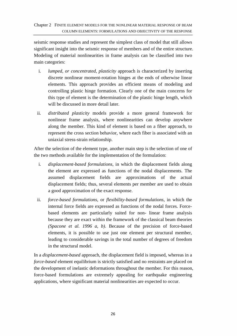
Two-Point Gauss–Radau Integration
The two previous methods confirm that it is not possible to satisfy all the three criteria by performing one-point integration for each plastic hinge region. Therefore, it is necessary to investigate two-point integration methods. Two-point Gauss–Legendre integration over each plastic hinge region gives the desired level of element integration accuracy; however, there are no integration points at the element ends. Two-point Gauss–Lobatto integration over the hinge regions places integration points at the element ends, but is not exact for the case of a linear curvature distribution. An alternative two-point integration rule is based on Gauss–Radau quadrature (Hildebrand, 1974 [39]). It is similar to Gauss–Lobatto, but it has an integration point at only one end of an interval rather than at both
ends. This gives Gauss–Radau quadrature an accuracy of 2-Y − 2, one order higher than that for Gauss– Lobatto. As a result, two Gauss–Radau integration points in each plastic hinge region gives the exact integration for an element with a linear curvature distribution. On the interval [0, 1], the two-point Gauss–Radau integration rule has integration points at [0, 2/3] with corresponding integration weights [1/4, 3/4]. The mapping of this integration rule to the plastic hinge
Chapter 2 FINITE ELEMENT MODELS FOR THE NONLINEAR MATERIAL RESPONSE OF BEAM
COLUMN ELEMENTS: FORMULATIONS AND OBJECTIVITY OF THE RESPONSE
36
regions at the element ends gives four integration points, ) = [0, 2EFV/3, � −2EF]/3, �], along with the respective weights, * = [EFV/4, 3EFV/4, 3EF]/4, EF]/4], Figure 2.5. This integration method satisfies the first criterion and the second, but criterion three, is not satisfied, because strain softening will result in localization within the plastic hinge region. The characteristic length over which the localized deformations are integrated will be equal to the integration weight, EY /4, assigned to the integration point at the element end rather than the plastic
hinge length, EY. This reduction in the characteristic length will cause the element to unload at a faster rate than expected to maintain equilibrium.
Modification of Two-Point Gauss–Radau Integration
By making the integration weights equal to EFV and EF], rather than EFV/4 and EF]/4,
it is possible to ensure that the localized deformations are integrated over a plastic hinge length. To this end, the two-point Gauss–Radau integration rule is applied over lengths of 4lpI and 4lpJ at the element ends, as shown in Figure 2.5 – b), thus giving the
integration point locations ) = [0,8EFV/3, L − 0,8EF]/3, L] and weights * =[ EFV , 3EFV , 3EF], EF]]. Nonlinear constitutive behavior is confined to the integration
points at the element ends only, while the section response at the two interior integration points is assumed linear elastic, with the same properties as those
defined by �RQ. With this modification of Gauss–Radau, plasticity is confined to a single integration point at each end of the element. The representation of linear curvature distributions is exact, furthermore, the characteristic length will be equal to the specified plastic hinge length when deformations localize due to strain-softening behavior in the hinge regions. Hence, all the three criteria introduced in paragraph 2.1.3., are met by the presented modification of the two-point Gauss–Radau plastic hinge integration method for force-based beam–column elements. In conclusion the modified Gauss–Radau quadrature method overcomes the difficulties that arise with Gauss–Lobatto integration for strain-softening behavior in force-based beam–column finite elements. The integration method confines material nonlinearity to the element ends over specified plastic hinge lengths, maintains the correct numerical solution for linear curvature distributions, and ensures objective response at the section, element, and structural levels.
Chapter 2 FINITE ELEMENT MODELS FOR THE NONLINEAR MATERIAL RESPONSE OF BEAM
COLUMN ELEMENTS: FORMULATIONS AND OBJECTIVITY OF THE RESPONSE
37
Figure 2.5 - a) Two-Point Gauss-Radau; b) Modified Gauss-Radau
2.1.4. Plastic hinge length determination (Priestley, Calvi, Seible, 1996)
The length of the plastic hinge, lp, for concrete elements has been an object of study and experimental work, since the second half of the fifties. Literature offers many, in some cases pretty different, formulas to evaluate lp. In the work carried out for the present thesis, the plastic hinge length is not a variable parameter, it is been decided to assume a plastic hinge length that would be used throughout all the analyses. The length used was computed on the basis of the work of Priestley,
Calvi, Seible, 1996 [15]. According to this formula the length of the plastic hinge, lp, is function of the characteristics of the reinforcement used, ultimate strength, yield strength and bars diameter, and of the length from the critical section to the point of contra-flexure in the member. The concept of plastic hinge, is based on the assumption that over the length lp, strain and curvature are considered to be equal to the maximum value at the
Chapter 2 FINITE ELEMENT MODELS FOR THE NONLINEAR MATERIAL RESPONSE OF BEAM
COLUMN ELEMENTS: FORMULATIONS AND OBJECTIVITY OF THE RESPONSE
38
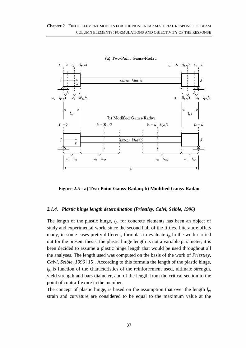
column base. The plastic hinge length incorporates the strain penetration length lsp, see Figure 2.6. lsp can be calculated as follow
(2.14) ERF = 0,156bQ�c3 being 6bQ the yield strength in ksi (kilopounds per square inches) and �c3 the
diameter of the longitudinal reinforcing bars. The curvature distribution is assumed to be linear for the remaining length, along the height of the column. This assumption refers to the bilinear approximation of the moment-curvature response, which somehow takes into account the displacement resulting from tension shift, and partially for shear deformation. Finally, the plastic hinge length, lp, might be computed as
(2.15) �F = d�8 + �RF ≥ 2�RF
(2.16) d = 0,2(6f/6b − 1) ≤ 0,08
�8 is the length from the critical section to the point of contra-flexure in the
member, i.e. the moment equal to zero. The double-curvature case , thus �8 =H/2 , being H the actual length of the member, prevails in the analyses of buildings under lateral loads. On the other hand, some structural members such as cantilevers experience single curvature, and the plastic hinge forms at one end only. Such is the case of bridge piers subjected to seismic loads in the transverse direction, see Figure 2.6 – a). Through the parameter k, it is emphasized the importance of the ratio of ultimate
tensile strength 6f to yield strength 6b of the longitudinal reinforcement. A high
value of k means that the plastic deformations spread away from the critical section as the reinforcement at the critical section strain-hardens, increasing the
plastic hinge length. If the ratio 6f/6b of the flexural reinforcement is low,
plasticity concentrates close to the critical section. The result is, therefore, a short plastic hinge length. In Figure 2.6 the length from the critical section to the point
of contra-flexure �8 is equal to the height of the member, in this case the plastic
hinge length EF obviously results larger than 2ERF . EF = 2ERF applies when �8 is
short. It implies strain penetration down into the foundation and also up into the column.
Chapter 2 FINITE ELEMENT MODELS FOR THE NONLINEAR MATERIAL RESPONSE OF BEAM
COLUMN ELEMENTS: FORMULATIONS AND OBJECTIVITY OF THE RESPONSE
39
Figure 2.6 – a) Idealization of curvature Distribution; b) Curvature distribution along a beamWithHinges element, from pushover analysis
Chapter 2 FINITE ELEMENT MODELS FOR THE NONLINEAR MATERIAL RESPONSE OF BEAM
COLUMN ELEMENTS: FORMULATIONS AND OBJECTIVITY OF THE RESPONSE
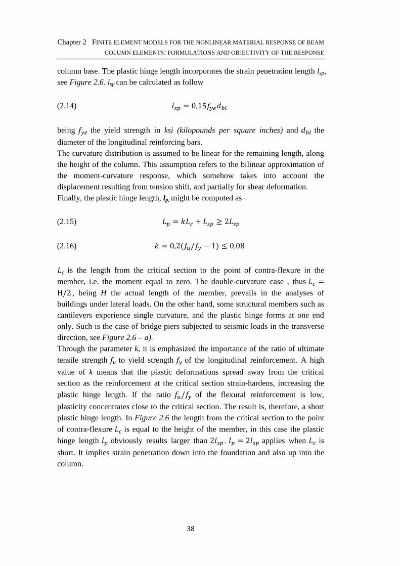
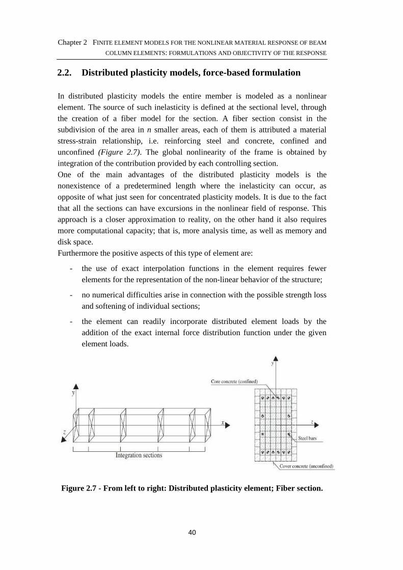
In distributed plasticity models the entire member is modeled as a nonlinear element. The source of such inelasticity is defined at the sectional level, through the creation of a fiber model for the section. A fiber section consist in the subdivision of the area in n smaller areas, each of them is attributed a material stress-strain relationship, i.e. reinforcing steel and concrete, confined and unconfined (Figure 2.7). The global nonlinearity of the frame is obtained by integration of the contribution provided by each controlling section. One of the main advantages of the distributed plasticity models is the nonexistence of a predetermined length where the inelasticity can occur, as opposite of what just seen for concentrated plasticity models. It is due to the fact that all the sections can have excursions in the nonlinear field of response. This approach is a closer approximation to reality, on the other hand it also requires more computational capacity; that is, more analysis time, as well as memory and disk space. Furthermore the positive aspects of this type of element are:
- the use of exact interpolation functions in the element requires fewer elements for the representation of the non-linear behavior of the structure;
- no numerical difficulties arise in connection with the possible strength loss and softening of individual sections;
- the element can readily incorporate distributed element loads by the addition of the exact internal force distribution function under the given element loads.
Figure 2.7 - From left to right: Distributed plasticity element; Fiber section.
Chapter 2 FINITE ELEMENT MODELS FOR THE NONLINEAR MATERIAL RESPONSE OF BEAM
COLUMN ELEMENTS: FORMULATIONS AND OBJECTIVITY OF THE RESPONSE
41
2.2.1. Element Formulation (Spacone et al. 1996) [16]
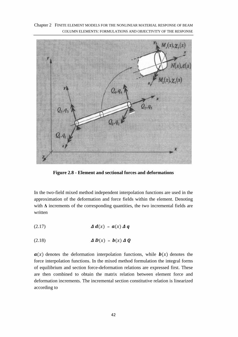
As just seen for the concentrated plasticity model, we are now considering beam-column elements formulated in a basic system without rigid-body displacement modes. The element provided of its local reference system x,y,z, is subdivided into a discrete number of cross sections, (Figure 2.7), located at the control points of the numerical integration scheme about to be introduced. The only source of non-linearity derives from the material constitutive laws. Some hypotheses need to be introduced in order to have in mind the framework of the formulation. In particular, the assumption of linear geometry, plane sections normal to the longitudinal axis during the element deformation history remain plane. Follows that all stress and strains are parallel to the longitudinal axis, which is the axis that connects the centroid of all the sections. The assumption of plane sections remain plane, is acceptable for small deformation in the case of homogeneous material, but it is also extended to the case of reinforced concrete elements, which is not an homogeneous material and it is characterized by phenomena like cracking and bond-slip. Shear effects are neglected, which is reasonable considering the ratio length to dept of the element being large. Torsion is assumed to remain linear elastic and uncoupled from the flexural and the axial response. Before discussing the formulation itself in more detail, it is necessary to introduce the following vectors, whose components can be identified in Figure 2.8:
Element force vector i = jiT i; ik ilimn Element deformation vector o = joT o; ok olomn
Being v the curvature and : the axial strain. The two-field mixed method uses the integral form of equilibrium and section force-deformation relations to derive the matrix relation between element generalized forces and corresponding deformations. The section force-deformation relation is linearized about the present state and an iterative algorithm is used to satisfy the non-linear section force-deformation relation within the required tolerance. In the following, the steps of the iterative algorithm are denoted by superscript j .
Chapter 2 FINITE ELEMENT MODELS FOR THE NONLINEAR MATERIAL RESPONSE OF BEAM
COLUMN ELEMENTS: FORMULATIONS AND OBJECTIVITY OF THE RESPONSE
42
Figure 2.8 - Element and sectional forces and deformations
In the two-field mixed method independent interpolation functions are used in the approximation of the deformation and force fields within the element. Denoting with ∆ increments of the corresponding quantities, the two incremental fields are written
(2.17) x y( ) = z( ) x �
(2.18) x {( ) = ( ) x |
z( ) denotes the deformation interpolation functions, while ( ) denotes the force interpolation functions. In the mixed method formulation the integral forms of equilibrium and section force-deformation relations are expressed first. These are then combined to obtain the matrix relation between element force and deformation increments. The incremental section constitutive relation is linearized according to
Chapter 2 FINITE ELEMENT MODELS FOR THE NONLINEAR MATERIAL RESPONSE OF BEAM
COLUMN ELEMENTS: FORMULATIONS AND OBJECTIVITY OF THE RESPONSE
43
(2.19) xy}( ) = �}��( )x{}( ) + ~}��( ) where �}�� and ~}�� are the section flexibility and residual deformations from the previous iteration. The residual deformations can, thus, be interpreted as the linear approximation to the deformation error that arises in the linearization of the section force-deformation relation. The weighted integral form of equation
Substituting � �( ) and � p( ) into the Eq. 2.20, for any �i, the integral is equal to
(2.21) �x�} − �}��x |} − �}�� = �
where T is a matrix that depends only on the interpolation functions, F is the element flexibility matrix, and s is the element residual deformation vector
(2.22) � = � �( )z( )� ��
(2.23) � = � �( )�( )( )� ��
(2.24) � = � �( )~( )� ��
In the classical two-field mixed method the integral form of the equilibrium equation is derived from the virtual displacement principle
(2.25) � �y�( )[x{}��( ) + x{}( ) ] � = ��� |}��
where �{��T( ) + �{�( ) represents the new internal force distribution. |� is the vector of nodal forces as previously defined. Recalling the definition of the
two incremental fields � y( ) and � {( ) , and knowing that the previous
equation must hold true for any ��u , it is possible to rewrite the equation in matrix form
(2.26) ��|}�� + ��x|} = |}
Chapter 2 FINITE ELEMENT MODELS FOR THE NONLINEAR MATERIAL RESPONSE OF BEAM
COLUMN ELEMENTS: FORMULATIONS AND OBJECTIVITY OF THE RESPONSE
44
From Eq. 2.21 and 2.26 the following equation in matrix form results
(2.27) −�}�� ��� �� �x|}x�} � = � �}��|} − ��|}��� The first equation is then solved for �|� and substituted into the second equation, obtaining
(2.28) ��[�}��]��(�x�} − �}��) = |} − ��|}��
The interpolation functions z( ) and ( ) selection and the peculiar selection of
deformation and force resultants q and Q, leads to � = �, the 3x3 identity matrix. This simplify the last expression into the linearized matrix relation between the
element forces �|� and the corresponding deformation increments K��� − ���TL
(2.29) [�}��]��(x�} − �}��) = x|} [���T]�T is the stiffness matrix. This form of writing the stiffness matrix
highlights that the starting point of the formulation is the flexibility matrix �.
2.2.2. Element and Section state determination
In a flexibility-based element, the element stiffness matrix is derived by inverting the flexibility matrix; thus, the element forces present the biggest challenge because they cannot be derived straightforward from the section forces. Spacone
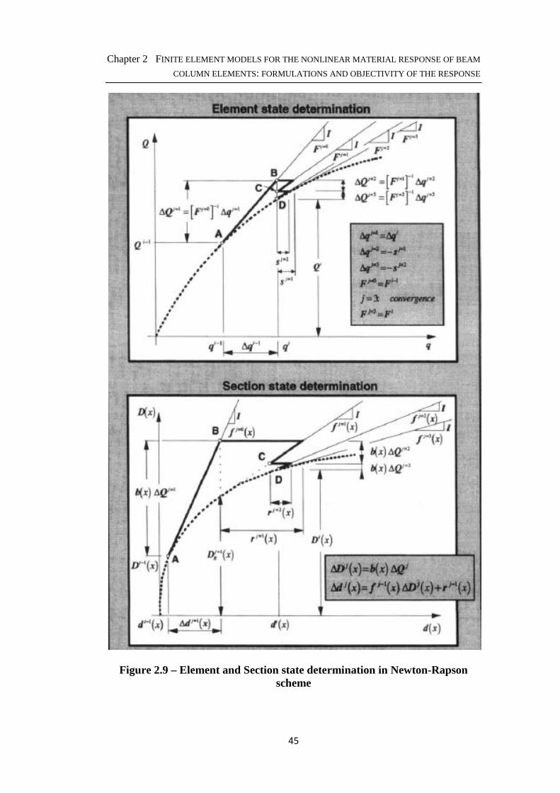
et al. introduce an iteration scheme similar to Newton-Rapson. The Newton-Rapson iteration scheme is used for the solution of the global equilibrium equation, at the structural level. Forces increments are applied, at the structural degrees of freedom, and Newton-Rapson is used to reduce the unbalanced forces to sufficiently small values at each iteration step. The solution of these equations leads to displacement increments at the end nodes of each element. The method about to be introduced is formulated for the element level. In fact, the iterations during the element state determination phase of the algorithm intend to reduce the deformation residuals to sufficiently small values. Figure 2.9 shows the element and section state determination in the Newton-Rapson scheme at structural level.
Chapter 2 FINITE ELEMENT MODELS FOR THE NONLINEAR MATERIAL RESPONSE OF BEAM
COLUMN ELEMENTS: FORMULATIONS AND OBJECTIVITY OF THE RESPONSE
45
Figure 2.9 – Element and Section state determination in Newton-Rapson scheme
Chapter 2 FINITE ELEMENT MODELS FOR THE NONLINEAR MATERIAL RESPONSE OF BEAM
COLUMN ELEMENTS: FORMULATIONS AND OBJECTIVITY OF THE RESPONSE
46
The element resisting forces for the current element deformations, at the i-th Newton-Rapson step, are
(2.30) �% = �%�� + ∆�% Now an iterative process internal to the i-th step of Newton-Rapson is introduced,
being the first iteration � = 1 and � = 0 is the i-th−1 step. The latter is the point A in Figure 2.9 and it represents the initial state of the element. The element force increments writes
(2.31) ∆|}#� = [�}#�]��∆�}#�
being [��#<]�T the initial element tangent stiffness matrix, ∆��#T the given element deformation increments.
Thus, it is possible to write the section deformation increments ∆y�#T( ), through
the linearization of the section force-deformation relation, having ∆{�#T( ) section force increments.
(2.32) ∆y}#�( ) = �}#�( )∆{}#�( )
In point B the section deformations are updated to y�#T( ) = y+�T( ) +∆y�#T( ), and the section stiffness and resisting forces corresponding to the new deformation sate need to be computed. This corresponds to the section state determination, that will be discussed later in the paragraph. From the assumption of plane sections remain plane and orthogonal to the longitudinal axis, follows the
derivation of the strain distribution in the section, :�#T( , �, �), and thanks to the constitutive law of concrete and steel, the derivation of the corresponding stresses ��#T( , �, �) and tangent modulus ��#T( , �, �). The latter are integrates over the
cross section area to obtain the section resisting forces ���#T( ) and the stiffness
matrix ��#T( ). The flexibility matrix, ��#T( ), is obtained inverting the stiffness matrix. The unbalanced forces at the section are the difference between the applied forces and the resisting forces; multiplying the unbalanced forces with the current
section flexibility gives residual deformations ��#T( ). They represents the linear approximation to the deformation error that arises in the linearization of the section force-deformation relation. The use of the tangent flexibility matrix in the
Chapter 2 FINITE ELEMENT MODELS FOR THE NONLINEAR MATERIAL RESPONSE OF BEAM
COLUMN ELEMENTS: FORMULATIONS AND OBJECTIVITY OF THE RESPONSE
47
model guarantees the fastest convergence, even thought any flexibility matrix could be used.
(2.33) {�}#�( ) = {}#�( ) − {�}#�( )
(2.34) ~}#�( ) = �}#�( ){�}#�( )
The residual element deformations are computed integrating the residual section deformations over the element length
(2.35) �}#� = � �( )~}#�( �� )�
The point B in Figure 2.9, describes the section and element state reached. Up to this point the first iteration loop is complete. The existence of residual element deformations violates the compatibility at
element nodes. Here the deformations should be equal to �+. In order to restore
compatibility corrective forces equal to – [�}#�]�T�}#� must be applied at the element ends. Furthermore, a corresponding force increment equal to – ( )[�}#�]�T�}#� is applied at all integration points of the element inducing a
deformation increment – �}#�( )[�}#�]�T�}#�. Therefore, at iteration � = 2 the state of the element is the following:
At each iteration new residual section deformations, and residual element deformations are updated. Convergence is achieved when the selected element convergence criterion is achieved. In Spacone et al. formulation the convergence
is based on an energy test. The energy measure ���� is used for the purpose and the element iterations converge if
(2.36) R����R�
∆���� �� ≤ ¡¢EE£¤¥¦§£ (6¢¤ � > 1)
Chapter 2 FINITE ELEMENT MODELS FOR THE NONLINEAR MATERIAL RESPONSE OF BEAM
COLUMN ELEMENTS: FORMULATIONS AND OBJECTIVITY OF THE RESPONSE
48
The element equilibrium is always satisfied during the element determination in the non-linear analysis, because the section forces are derived from the element forces by means of interpolating functions. Whereas, the section force-deformation and the element force-deformation relations are only satisfied within a tolerance, when convergence is reached. Therefore, during the iterations the element forces approach the value corresponding to the imposed deformation, while strictly satisfying element equilibrium at all times. As for the element state determination, the section state determination includes the
located at point (y, z) the strains are described as :( , �, �) = I(�, �)y( ), being I(�, �) = j−� � 1n a simple geometric vector. Given the constitutive laws of the
materials,�( , �, �) and �( , �, �) can be derived from the strain distribution. The
tangent material modulus � and the stress distribution � are needed to determine
the section stiffness matrix �( ) and the resisting forces {�( ) , computed through the virtual force principal. In particular, using a computer program requires the selection of a numerical integration scheme. The one used in this case, where a section at location x is subdivided into n(x) fibres, the midpoint integration rule is used for the following integrals
(2.37) �(") = � I�(�, �)ª( , �, �)I(�, �)y««(")
(2.38) {(") = � I�(�, �)¬( , �, �)y««(")
Being the number of fibres a discrete number, the two integrals are transformed into a summation. The accuracy of such computations depends on the number and location of fibres, in fact, too little fibres could cause the underestimation of section capacity. In the other hand, increasing the number of fibres is computationally expensive. Thus, there must be the right balance between accuracy and computation effort.
2.2.3. Numerical integration
Gauss-Lobatto integration scheme is used to evaluate the integrals Eq. 2.22 and Eq. 2.23. This procedure is superior to the classical Gauss integration scheme because it always includes the end sections of the integration domain. When no distributed load act on the element, the end sections are those subjected to the
Chapter 2 FINITE ELEMENT MODELS FOR THE NONLINEAR MATERIAL RESPONSE OF BEAM
COLUMN ELEMENTS: FORMULATIONS AND OBJECTIVITY OF THE RESPONSE
49
largest forces and undergo the largest inelastic excursions. Therefore, monitoring the end sections results in more accuracy of the non-linear response of the element. The m-th order Gauss-Lobatto integration scheme permits exact integration of
polynomials of order up to (2 − 3), and it is based on the following scheme
2.2.4. Loss of objectivity at section and element levels (Coleman and Spacone, 2001)[12]
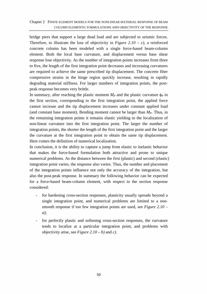
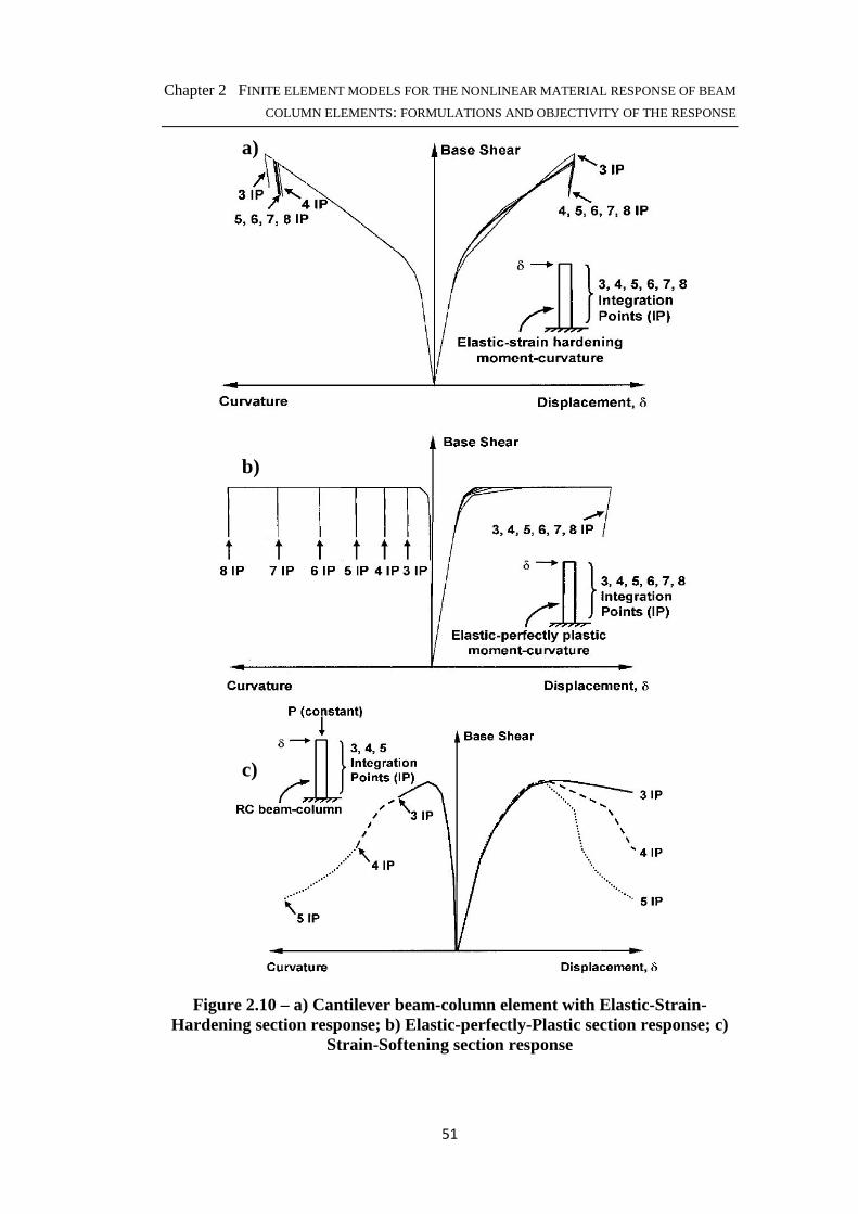
In the case of a strain-hardening section behavior, objectivity is guaranteed both at section and element level, as long as more than three integration points are used. To prove this, the case of a cantilever single beam-column element under an imposed transverse tip displacement has been considered by Coleman and
Spacone, 2001 [12]. Figure 2.10 – a) shows the response of the force-based element, on the left base curvature (curvature of the first integration point) versus base shear, on the right displacement versus base shear. The peak point identifies the displacement reached before unloading. From Figure 2.10 – a) is possible to note how the response is objective at both the element and section levels for models with four or more integration points. Three integration points do not accurately integrate the element integrals; thus, the stiffness over-prediction in the strain-hardening region. The same test is carried out in the case of elastic perfectly plastic moment-curvature behavior. Here, prediction of the element force-displacement response remains objective while the peak curvature demand varies with the number of integration points, Figure 2.10 – b). The loss of objective curvature prediction is related to the localization of the inelastic curvature at the base integration point. When this bottom section reaches the plastic moment, the column reaches its load-carrying capacity. As the tip displacement increases, the curvature of the base integration point increases with constant (plastic) moment, while, along the length of the column, all the other integration points remain linear elastic and do not see any change in either curvature or moment. The length of the base integration point, and so the plastic hinge length, becomes a function of the number of integration points used. As the number of integration points increases, the plastic hinge length decreases, and the curvature demand in the base integration point must increase to yield the same prescribed tip displacement. Anyhow, the loss of objectivity is more evident in the case of strain-softening section behavior. Softening might happen in reinforced concrete columns or in
Chapter 2 FINITE ELEMENT MODELS FOR THE NONLINEAR MATERIAL RESPONSE OF BEAM
COLUMN ELEMENTS: FORMULATIONS AND OBJECTIVITY OF THE RESPONSE
50
bridge piers that support a large dead load and are subjected to seismic forces. Therefore, to illustrate the loss of objectivity in Figure 2.10 – c), a reinforced concrete column has been modeled with a single force-based beam-column element. Both the local base curvature, and displacement versus base shear response lose objectivity. As the number of integration points increases from three to five, the length of the first integration point decreases and increasing curvatures are required to achieve the same prescribed tip displacement. The concrete fiber compressive strains in the hinge region quickly increase, resulting in rapidly degrading material stiffness. For larger numbers of integration points, the post-peak response becomes very brittle. In summary, after reaching the plastic moment MP and the plastic curvature ϕP in the first section, corresponding to the first integration point, the applied force cannot increase and the tip displacement increases under constant applied load (and constant base moment). Bending moment cannot be larger than MP. Thus, in the remaining integration points it remains elastic yielding to the localization of non-linear curvature into the first integration point. The larger the number of integration points, the shorter the length of the first integration point and the larger the curvature at the first integration point to obtain the same tip displacement. Here comes the definition of numerical localization. In conclusion, it is the ability to capture a jump from elastic to inelastic behavior that makes the force-based formulation both attractive and prone to unique numerical problems. As the distance between the first (plastic) and second (elastic) integration point varies, the response also varies. Thus, the number and placement of the integration points influence not only the accuracy of the integration, but also the post-peak response. In summary the following behavior can be expected for a force-based beam-column element, with respect to the section response considered:
- for hardening cross-section responses, plasticity usually spreads beyond a single integration point, and numerical problems are limited to a non-smooth response if too few integration points are used, see Figure 2.10 –
a);
- for perfectly plastic and softening cross-section responses, the curvature tends to localize at a particular integration point, and problems with objectivity arise, see Figure 2.10 – b) and c).
Chapter 2 FINITE ELEMENT MODELS FOR THE NONLINEAR MATERIAL RESPONSE OF BEAM
COLUMN ELEMENTS: FORMULATIONS AND OBJECTIVITY OF THE RESPONSE
51
Figure 2.10 – a) Cantilever beam-column element with Elastic-Strain-Hardening section response; b) Elastic-perfectly-Plastic section response; c)
Strain-Softening section response
a)
b)
c)
Chapter 2 FINITE ELEMENT MODELS FOR THE NONLINEAR MATERIAL RESPONSE OF BEAM
COLUMN ELEMENTS: FORMULATIONS AND OBJECTIVITY OF THE RESPONSE
52
2.2.5. Regularization techniques
Constant fracture energy criterion
The previous paragraph arose the problem of deformation localization, thus, the need of techniques that regularize the element formulation. The objective is to obtain a stable method, independent of the section stress-strain behavior. As introduced in paragraph 2.1.2. the concept of constant fracture energy is now applied to a force-based beam element that softens in compression. Therefore, it is necessary to define a new parameter, known as the fracture energy in compression C?±; σ is the concrete stress,³+ is the inelastic displacement, εµ the inelastic strain, Lµ¶ is the length of the softening integration point. C?± is defined as follows, and
represents the area under the post-peak portion of compressive stress-displacement curve, in Figure 2.3,
(2.40) ·�̧ = � ¬ y¹% = ¯ � ¬ yº% = �%( � ¬ yº% Recalling Eq.2.8, and assuming C?± is known from experimental tests, it is
possible to note that theoretically the constitutive law must be calibrated for each separate integration point. In practice, plastic hinges normally form at the element ends, where the extreme integration points lie. If all elements in a model are
integrated with the same scheme and number of integration points, :;< only varies for elements of different length L. In this way the constitutive law is linked to the element length, which is a straightforward process. As the number of integration points increases, larger inelastic strains to satisfy the constant fracture energy criteria are needed at the end integration point. This is equivalent to assuming a constant stress-displacement relation rather than a constant stress-strain law.
Curvature post-processing
After the regularization of the global force-displacement response, in some cases there is still a need to post-process the results to obtain an objective prediction of the curvature demand in the plastic hinge region. This is due to the fact that This is due to the fact that the plastic zone length is the length of the first integration point and does not necessarily correspond to the physical length of the plastic hinge.
Chapter 2 FINITE ELEMENT MODELS FOR THE NONLINEAR MATERIAL RESPONSE OF BEAM
COLUMN ELEMENTS: FORMULATIONS AND OBJECTIVITY OF THE RESPONSE
53
A simple procedure is presented by Coleman and Spacone, 2001 [12]. The first consideration is that the total curvature in the plastic hinge region can be
separated into elastic and inelastic curvature components as » = »Q + »+ , and
that the inelastic hinge rotation is given by ¼+ = »+�+.. The inelastic curvature of the model, output of the analysis, can be approximated as
(2.41) »+½¾¿Q3 ≅ ÁÂÃÂÄ9ÅÆ�ÅÂÄÆ B
The above formula is needed to compute the scale factor, with which the inelastic curvature of the model will be weighted, to obtain the final actual curvature, after this regularization process. Scale factor is
(2.42) �§¥E£ 6¥§¡¢¤ = ÇÂ4ÃÆ(T�ÇÂ4)Ã4(Ã�Ã4)
Finally, the objective prediction of the curvature
(2.43) » = »Q + »+½¾¿Q3 ∗ (�§¥E£ 6¥§¡¢¤)
In conclusion, for a force-based beam element it appears that if the length of the first integration point corresponds to the length of the plastic hinge, i.e., if �+. = �F, no post-processing of the curvature is needed because the curvature is
objectively predicted by the element. On the other hand, selecting the number of
Gauss-Lobatto integration points in such a way that �+. ≅ �F may cause two
problems:
- the number of integration points may be too small for short elements (causing undesirable reduced integration) or too large for long elements (increasing the computational cost of the element);
- in most cases, the length of the element would also have to be adjusted, thus introducing an additional element in each member. This greatly increases the computational cost of the analyses.
Different integration schemes in which the user can define the length of the integration points would also solve the issue, but would significantly compromise the accuracy of the numerical integration. The regularization approach described in this paper is general and does not affect either the element formulation or the integration scheme.
Chapter 2 FINITE ELEMENT MODELS FOR THE NONLINEAR MATERIAL RESPONSE OF BEAM
COLUMN ELEMENTS: FORMULATIONS AND OBJECTIVITY OF THE RESPONSE
54
Chapter 3
EXISTING STRUCTURE AND MODELING ISSUES
3.1. The bridge: Jamboree Road Overcrossing
The Jamboree Road Overcrossing (JRO) is located in the Orange County, in the city of Irvine on Route 261. The route is part of the Eastern Transportation Corridor, one of the design/build/operate toll roads in Southern California (Figure
3.1 – a). The geographical coordinates of the location are +33° 43' 10.08", -117° 47' 43.26". The bridge is object of a project of health monitoring by the research group of Professor Maria Q. Feng, University of California Irvine [18]. The JRO can be considered an Ordinary Standard Bridge, in fact, it meets the requirements of Caltrans Seismic Design Criteria provided to define such category. The JRO is a typical three-span continuous cast-in-place pre-stressed post-tension box-girder (Figure 3.1 - b) [17]. The total length of the bridge is 366 ft (110,9 m), in which the lengths of the spans are 114, 152 and 100 ft (35,5 m, 46,1 m and 30,3
m), respectively from span 1 to 3 [22] (Figure 3.1 - c). The super-structure consists of a two-cell cast-in-place pre-stressed and post-tensioned box girder, which is supported on two monolithic single columns and sliding bearings on both abutments. The sliding bearings allow creep, shrinkage, and thermal expansion or contraction. On the outer edges of both traffic lanes, a concrete barrier approximately 1.75 ft (0.8 m) high is provided. The typical cross section of the box-girder is shown in Figure 3.1 - d).
Chapter 3 THE EXISTING STRUCTURE AND THE MODELING ISSUES
56
The columns are rectangular with circular ends and interlocking spiral reinforcement. The columns height is 26,126 ft and 28,41 ft (7,96 m and 8,66 m). The shortest bent is usually referred to as left bent, while the taller is the right bent. The cross-section width is 8,25 ft (2,51 m) and its depth is 5,5 ft (1,67 m). Both columns are continuous with the box girder due to the main bent reinforcement being anchored in solid concrete diaphragms filling the girder void at bent locations. Each bent is founded on a square reinforced concrete (RC) pad footing supported in turn on Caltrans class 100C piles. Similarly, the abutments are founded on pad footings supported on class 100C piles. The JRO Bridge was designed by the Transportation Corridor Agencies in accordance with the American Association of State Highway and Transportation
Officials (AASHTO) 1983 Standard Specifications for Highway Bridges [19] with interims and revisions by Caltrans. The construction of the JRO bridge was completed in 2001.
a)
Chapter 3 THE EXISTING STRUCTURE AND THE MODELING ISSUES
57
Figure 3.1 - a) Jamboree Road Overcrossing located on Route 261; b) Plan; c) Elevation; d) Typical Cross Section Box-Girder
Chapter 3 THE EXISTING STRUCTURE AND THE MODELING ISSUES
58
3.2. The OpenSees modeling
3.2.1. The software OpenSees
The software OpenSees [20], the Open System for Earthquake Engineering
Simulation, is an object-oriented, open source software framework. It has been developed by PEER (Pacific Earthquake Engineering Research Center), one of the most important American research institutes for seismic engineering. The software allows users to create both serial and parallel finite element computer applications for simulating the response of structural and geotechnical systems subjected to earthquakes and other hazards. OpenSees is primarily written in C++ and uses several Fortran and C numerical libraries for linear equation solving, and material and element routines. It is an open source software, that means it is free and it can be modified and improved by anyone. OpenSees is based on the TCL, Tool Command Language, that supports, other than specific commands of the software, basic operations and file manipulation. The construction of the finite element model and the following analysis are, therefore, written as command lines; in fact, the software does not have a graphical interface. Because of this, it is barely usable in every day’s practice, but a very powerful tool in the research field. OpenSees executes both static and dynamics analysis, linear and non-linear. Four different phases can be identified as the basic process for each analysis:
a. ModelBuilder Object: the characteristics of the physical model to be analyzed are defined, both plane models and three-dimensional;
b. Domain Object: nodes, elements, sections, materials, restraints, masses and loads are defined and recorded, available for all the following analysis;
c. Analysis Object: the numerical procedure to be used is defined, the solving algorithm, the integrator, convergence tests, the integration steps. Analysis objects encapsulate algorithms that direct the Domain components to form and solve the governing equations of structural equilibrium at each integration step;
d. Recorder Object: records and store into output files the structural response obtained through the analysis.
To follow, in Figure 3.2 [21], the modeling hierarchy for nonlinear structural analyses on which the software OpenSees is based.
Chapter 3 THE EXISTING STRUCTURE AND THE MODELING ISSUES
59
Figure 3.2 - Modeling hierarchy for nonlinear analyses [21]
Chapter 3 THE EXISTING STRUCTURE AND THE MODELING ISSUES
60
3.2.2. The Three-Dimensional Model
Unit and Coordinate Systems
A three-dimensional (3D) model of the structural system is required to capture the response of the entire bridge system and individual components under specific seismic demand characteristics. The interaction between the response in the orthogonal bridge directions and the variation of axial loads in column bents throughout the analysis is captured more accurately in a 3D model, rather than a 2D model. The 3D linear model will be the basis for the nonlinear one. Having a 3D model enables correct evaluation of the capacity and ductility of the system under seismic loads or displacements applied along any given direction, not necessary aligned with the principal axis of the bridge. The United States Customary System has been used for all the units used in the OpenSees model. Length are reported in feet (ft), weights in kilo-pounds (kips),
time in seconds (sec.). Other important derived and frequently used units are kilo-
pounds per square feet (ksf) for the elastic moduli, feet squares (ft2) for areas, feet to the power four (ft4) for inertia moments. The local and global coordinate system used for the modeling and analysis of the bridge is shown in Figure 3.3 a). The global X-axis is in the direction of the chord connecting the abutments, denoted as the longitudinal direction; the global Z-axis is orthogonal to the chord in the horizontal plane, representing the transverse direction; while the global Y-axis defines the vertical direction of the bridge. For the analysis and design of elements of the bridge using two-noded elements, a local coordinate system is used, as shown in Figure 3.3 - c).The orientation of all frame elements in the structure coincides with the positive direction of the global axis; namely, the coordinate of node i of the frame will be smaller than those of node j.
Mass distribution
All bridge elements will be approximated with a distributed mass along their length and assigns them as lumped mass at each node, based on tributary lengths. To approximate the distributed mass with lumped masses, a sufficient number of nodes and segments have to be defined. The weight of normal concrete is assumed
as � = 143.96 �/ �.�. No rotational mass have been taken into account.
Chapter 3 THE EXISTING STRUCTURE AND THE MODELING ISSUES
61
Figure 3.3 - Global and local coordinate system
Elements and restraints
As suggested by Caltrans guidelines [1], a minimum of three elements per column and four elements per span shall be used in a linear elastic model. In fact, 10 elements have been used for each of the span, from 1 to 3. A rigid link, in correspondence of the connection bent-deck, have been used, the rigid link goes from the top of the bent to the centroid of the superstructure. The different types of elements used for the columns will be discussed later. The boundary (support) conditions were defined as fixed at the base of each bent, thus the restraints for the three translational degrees of freedom are zero displacement imposed, and the restraints for the three rotational degrees of freedom are zero rotation imposed.
Chapter 3 THE EXISTING STRUCTURE AND THE MODELING ISSUES
62
Abutments
The modeling of the abutments is one of the most controversial issues when modeling highway bridges. Nowadays, researchers use different abutment models according to the purpose of the analysis. Although several studies have been conducted to study the abutment behavior, a lack of a unique idealization still persists. Abutments are earth-retaining systems designed to provide unimpeded traffic access to and from the bridge. Abutments also provide an economical means of resisting bridge inertial loads developed during ground excitations. Abutment walls are traditionally designed following principles for free-standing retaining walls based on active and passive earth pressure theories. However, such pressure theories are invalid for abutment walls during seismic events when inertial loading from the massive bridge structure induces higher than anticipated passive earth pressure conditions (Lam and Martin, 1986 [23]). A realistic abutment model should represent all major resistance mechanisms and components, including an accurate estimation of their mass, stiffness, and nonlinear hysteretic behavior. Values of embankment critical length and participating mass were suggested by many research studies in order to quantify the embankment mobilization. The consideration of the abutment system participating mass has a critical effect on the mode shapes and consequently the dynamic response of the bridge, captured primarily through time history analysis. The load pattern specified for a pushover analysis of the bridge is also adjusted due to this additional mass, modifying the force-deformation results of the system considerably. Due to the high sensitivity of the bridge response to the magnitude of the abutment mass, additional research is needed to standardize the modeling recommendations for Caltrans bridges. In addition, soil-structure interaction behind the abutment walls and due to the abutment foundations is also an important aspect affecting the abutment system behavior that requires further investigation. The main motivation to apply increasingly sophisticated abutment models is related to the accessibility to more powerful computers rather than an apparent inaccuracy of simpler models, but additional research is needed to standardize the modeling recommendations for bridges. Although different abutment models are available, in this thesis it is sufficient to model the abutment as a single spring was assigned to each degree of freedom, i.e. transverse, longitudinal, vertical, and their respective rotations, resulting in a total of 12 elastic springs in the bridge FE models [24]. The reason to use this model is to simplify the analysis and because the nonlinearity of the bridge under
Chapter 3 THE EXISTING STRUCTURE AND THE MODELING ISSUES
63
earthquake forces arises from different sources, such as the column plastic hinges, as explained later. The abutments ends are fixed, but a zeroLength element has been built in correspondence of the end nodes. To each of the two zeroLength element it has been associated the properties of the six elastic springs, to simulate the interaction between the bridge and the soil. The following values were assumed for both abutments:
Spring stiffness of Trans X direction !" = 4748,82 '() / �.
Spring stiffness of Trans Y direction !+ = 437913 '() / �.
Spring stiffness of Trans Z direction !- = 3974,95 '() / �.
Spring stiffness of Rot X direction 0" = 56453168 '() ∗ �./234
Spring stiffness of Rot Z direction 0+ = 647961,9 '() ∗ �./234
Spring stiffness of Rot Z direction 0- = 3941217 '() ∗ �./234
3.2.3. Modal Analysis and the definition of the load path for Pushover Analysis
Modal Analysis is the study of the dynamic properties of structures under vibrational excitation. It is executed on the linear elastic model, therefore elastic elements have been defined also for the bents. In structural engineering, modal analysis involves the use of both, a system mass matrix and a system stiffness matrix. The purpose is to estimate the natural frequencies (periods) and corresponding mode shapes associated to the dynamics of the system. These periods of vibration are very important to note in earthquake engineering, as it is desirable that a structure's natural frequency does not match the frequency of expected earthquakes in the region in which the building is to be constructed. If a structure's natural frequency matches an earthquake's frequency, the structure could continue to resonate and experience structural damage. The goal of modal analysis in structural mechanics is to determine the natural mode shapes and frequencies of an object or structure during free vibration. It is common to use the finite element method (FEM) to perform this analysis because, like other calculations using the FEM, the object being analyzed can have
Chapter 3 THE EXISTING STRUCTURE AND THE MODELING ISSUES
64
arbitrary shape and the results of the calculations are acceptable. The types of equations which arise from modal analysis are those seen in eigensystems. The physical interpretation of the eigenvalues and eigenvectors which come from solving the system are that they represent the frequencies and corresponding mode shapes. Sometimes, the only desired modes are the lowest frequencies because they can be the most prominent modes at which the object will vibrate, dominating all the higher frequency modes. For the most basic problem involving a linear elastic material which obeys Hooke's Law, the matrix equations take the form of a dynamic three dimensional spring mass system. The generalized equation of motion is given as:
(3.1) [6][89 ] + [;][8< ] + [=][8] = [>]
where [M] is the mass matrix, ?89 @ is the 2nd time derivative of the displacement
[U] (i.e., the acceleration), [8< ] is the velocity, [C] is a damping matrix, [K] is the stiffness matrix, and [F] is the force vector. The general problem, with nonzero damping, is a quadratic eigenvalue problem. However, for vibrational modal analysis, the damping is generally ignored, leaving only the 1st and 3rd terms on the left hand side:
(3.2) [6][89 ] + [=][8] = [0]
This is the general form of the eigensystem encountered in structural engineering using the FEM. To represent the free-vibration solutions of the structure harmonic
motion is assumed, so that ?89 @ is taken to equal ω2 [U], where ω2 is an eigenvalue
(with units of reciprocal time squared, [s – 2]), and the equation reduces to:
(3.3) [6][8] BC + [=][8] = [0]
This eigenvalues problem will provide the natural frequency of the system, through which it will be possible to compute the eigenvectors, physically represented by the mode shapes of the system, as mentioned before. The computed natural frequencies that will be reported to follow, derive from the analytical model with the boundary spring elements located in the abutments ends, and fixed ends for the columns, as mentioned before. The mode shapes corresponding to the computed natural frequencies of the bridge are plotted for the vertical direction and for the transverse direction, for the mode shapes 2.
Chapter 3 THE EXISTING STRUCTURE AND THE MODELING ISSUES
First mode shape does not have a transversal component, while the others do. To follow plots of mode shape 2 (Figure 3.4).
Since the first mode shape does not have any transversal component, the second mode shape has been considered when assigning a load path to the Pushover analysis. In fact the normalized eigenvectors have been computed, and the load path created has the transversal component of those values as load multipliers. This implies that the load path selected for the Pushover analysis follows the shape of the second vibration mode.
Figure 3.4 - Mode Shape 2, from top to bottom: plan, elevation and lateral view
Chapter 3 THE EXISTING STRUCTURE AND THE MODELING ISSUES
66
3.3. The prototype materials
3.3.1. Linear elastic material for the deck
A linear elastic material prototype has been created for the deck, with the following properties
Deck: Young's modulus O = 649584 '
Shear modulus Q = O4GH'/2,4 '
Some part of the model, require the elastic properties also for the bents. The elastic modulus and the shear modulus have been assumed to be equal to those used for the deck
Columns: Young's modulus O = 649584 '
Shear modulus Q = O4GH'/2,4 '
3.3.2. Elasto-plastic materials for the bents
When modeling concrete elements with nonlinear materials, one has to distinguish between unconfined and confined concrete. The first is associated to the cover concrete, confined by spiral hoops, while the second is associated with the core of the element. It is essential to incorporate an accurate model of the material behavior, because after the occurrence of destructive earthquakes, it has been observed one of the most damaged elements on highway bridges is a column.
Concrete01
One of the two concrete considered for modeling the columns is a material available in OpenSees named Concrete01. This command is used to construct a uniaxial Kent-Scott-Park concrete material object with degraded linear unloading/reloading stiffness according to the work of I. D. Karsan and J. O.
Jirsa (1969) [25] and no tensile strength. Concrete01 model is widely used because of its simplicity and the control that one has over the input parameters.
Chapter 3 THE EXISTING STRUCTURE AND THE MODELING ISSUES
67
The expected compressive strength for unconfined concrete is set equal to
720 ' , and equal to 1,5 ∗ 720 ' for confined concrete, according to Caltrans
recommendations. The confined strength has been raised to 1198 ' , to let the material be the most similar to Concrete07, which will be introduced later. The strains associated with these two peak stresses have been set equal to those of concrete07, while the Young Modulus in this model is obtained applying the following expression
(3.4) OS = 2 ∗ TUV
WV
where εc is the strain associated to f’ c, f’c is the expected compressive strength for concrete, and Ec is the tangent modulus of elasticity at the origin of coordinates. Once the compressive strength is reached, the unconfined stress falls rapidly to zero at the spalling strength, while the confined stress degrades not as rapidly as the unconfined stress. The confined concrete model should continue to ascend until the confined compressive strength f’ cu is reached. The segment should be followed by a descending curve dependent on the parameters of the confining steel, then a plateau for the confined concrete. The ultimate compressive strain should be the point where strain energy equilibrium is reached between the concrete and the confinement steel.
Concrete07
Many researchers have devoted a great effort in defining the stress-strain relation of concrete. Among the publications regarding this issue there are few that presented successful expressions for a stress-train relationship for concrete (Mander, et al. 1988 [26]; Chang and Mander 1994 [27]). The authors of Concrete07 model give the following reasons for having created such material model: the model considers wedging action in the cracks, which makes compression stress develop prior to crack closure; the model behaves differently depending on the moment when the strain reversal occurs, providing a more robust hysteretic behavior; the model proposed by J. B. Mander et al. (1988) [26] is widely used to determine the confined concrete properties and the model proposed by G. A. Chang and J. B.
Mander (1994) [27] extends this last J. B. Mander’s model to include the behavior
Chapter 3
of unconfined and high strength concrete; [27] used a large number of cyclic concrete tests to validate the model behavior.In Mander’s model the initial might be represented by the same equation,concrete, since the confining steel has no effect in this range of strains3.5). Mander’s model have been used to compute the yielding and the ultimate compressive strain for the confined concrete
(3.5) XSS =
(3.6) XSY =
Where fy is the yielding strength of the longitudinal reinforcing bars, ultimate strain of the longitudinal reinforcing bars. Considering that in the cross section of the bents it is possible to inscribe two circles formulas for circular cross sections, transversally reinforced with spiral hoops, have been used.
(3.7)
Z[\ is the cross section area of the spirals,
the spiral pitch, distance from center to center of the spirals.
Figure 3.
THE EXISTING STRUCTURE AND THE MODELING I
68
of unconfined and high strength concrete; G. A. Chang and J. B. Mander
used a large number of cyclic concrete tests to validate the model behavior.he initial ascending curve has the same initial slope
might be represented by the same equation, for both confined and unconfined since the confining steel has no effect in this range of strains
model have been used to compute the yielding compressive strain and the ultimate compressive strain for the confined concrete as follows
= XS ]1 : 5 ∗ ^TUVVT_V
` 1ab
� 1,4 c0,004 : d,e∗Tf∗gh∗WhiTUVV
j
is the yielding strength of the longitudinal reinforcing bars, ultimate strain of the longitudinal reinforcing bars. Considering that in the cross section of the bents it is possible to inscribe two circles formulas for circular cross sections, transversally reinforced with spiral hoops, have been used.
k[ � e∗lhmnh[
is the cross section area of the spirals, 4[ is the diameter of the core and
the spiral pitch, distance from center to center of the spirals.
Figure 3.5 - Mander's model for concrete
E AND THE MODELING ISSUES
G. A. Chang and J. B. Mander (1994) used a large number of cyclic concrete tests to validate the model behavior.
rve has the same initial slope, and for both confined and unconfined
since the confining steel has no effect in this range of strains (Figure
compressive strain
is the yielding strength of the longitudinal reinforcing bars, X[Y is the ultimate strain of the longitudinal reinforcing bars. Considering that in the cross section of the bents it is possible to inscribe two circles formulas for circular cross
is the diameter of the core and s is
Chapter 3 THE EXISTING STRUCTURE AND THE MODELING ISSUES
69
The main difference from Concrete01, is that Concrete07 is able to describe the tensile behavior of the material (Figure 3.6, tensile behavior, upper right part, and compressive behavior lower left part, are note not to scale). The eight parameter needed to the describe the material are introduced in Figure 3.6 and explained in more detail, to follow.
Figure 3.6 – Chang and Mander, Envelope and variable definition Concrete07
Unconfined Concrete – For unconfined concrete, the peak compressive strength fc in the above figure is f'c and corresponding strain ec is e'c. Assuming that the compressive strength for unconfined concrete is readily available, the key parameters required for the model can be found using the following recommendations which include (Chang and Mander, 1994, [27] units is psi):
′S � pqHrq (qG4 )G3' Hrs)2G (tG �2Gqu�ℎ
(3.8) G_S � TUVwx
eyyy
Chapter 3 THE EXISTING STRUCTURE AND THE MODELING ISSUES
70
(3.9) OS = 185000 ∗ _S
�/z
(3.10) { = 7,5 ∗ | _S
(3.11) X{ = { ∗ C}V
"\ = 2
"~ = 2.3
(3.12) 2 = TUV
��y − 1,9
Confined concrete – Confinement increases the strength and ductility of concrete. These effects are accounted in the above figure by replacing the peak compressive strength and the corresponding strain with f'cc and e'cc, respectively. The value of r is also decreased. The monotonic envelope for the tension side of the confined concrete follows the same curve that is used for unconfined concrete. The recommended approach to define all critical parameters needed to model the confined concrete under compression are as follows (Chang and Mander, [27] 1994):
′S = pqHrq (qG4 )G3' Hrs)2G (tG �2Gqu�ℎ;
(3.13) ′SS = ′S ∗ (1 + 'd ∗ "_)
(3.14) 'd = Z ∗ ]0.1 + y,�d��∗�Ub
(3.15) "_ = �d + T��C∗TUV
(3.16) G_Sy = TUV�
wx
eyyy
(3.17) Z = 6,886 − (0,6069 + 17,275�) ∗ G�e,�z��
(3.18) � = e,���[y,�ze��y,��y����,�����]�y,d
− 5
Chapter 3 THE EXISTING STRUCTURE AND THE MODELING ISSUES
71
(3.19) � = T�wT��
�G(qu �C ≥ �d
(3.20) XSS � XS ∗ (1 + 'C ∗ "_)
'C = 5 ∗ 'd (qr2s3 �2Gqu�ℎ �23q tG2 G 2G(q r2HGsGq�)
The actual stress-strain relationship used for Concrete07 in the model, is shown in Figure 3.7 –a) and b), where compressive stresses and strains are assumed to be negative. Stresses are plotted in ksf, while strains are plotted in %. In particular, Figure 3.7 a) shows the compressive behavior of concrete07:
- The dashed blue line is the stress-strain curve for the unconfined concrete;
after reaching ′S , the peek compressive strength of 720 ksf, the
descending branch starts and reaches f _SY , the ultimate compressive
strength, of 0 ksf, corresponding to the ultimate compressive strain εSY,, of 0,0635.
- In solid blue the stress-strain curve for the confined concrete, whose
yielding strength, ′SS, is equal to 1198 ksf. Here the descending branch
starts and reaches f _SSY, the ultimate compressive strength, of 1168 ksf,
corresponding to the ultimate compressive strain εSSY = 0,0142.
Figure 3.7 b) shows the tensile behavior of concrete07; the tensile stress-strain relationship is assumed to be equal for both unconfined and confined concrete. Figure 3.7 c) shows the superposition of concrete01 (in red) and concrete07 (in blue) curves. It should be remarked that for concrete01, the Young Modulus is not assigned from the user, therefore there is no control over this parameter. Here comes from the discrepancy between the two curves for the confined concrete. Results of pushover analysis have been compared for both concretes, but in the following considerations only concrete07 have been taken into account.
Chapter 3 THE EXISTING STRUCTURE AND THE MODELING ISSUES
72
a)
b)
Chapter 3 THE EXISTING STRUCTURE AND THE MODELING ISSUES
73
Figure 3.7 – a) Compressive behavior of Concrete07; b) Tensile behavior; c) Superposition of concret01 and concrete07 models. Not to scale.
Steel02
The Steel02 command is used to construct a uniaxial Giuffre-Menegotto-Pinto [28] steel material object, with isotropic strain hardening option. Six parameters are needed to define the model of the selected steel. The first two parameters needed are the Young’s Modulus E and the yield strength fy (reported also the
corresponding yield strain ε� ). The following values, corresponding to
Reinforcing Steel A706/A706M (Grade 60/Grade 400), have been assumed
Young's modulus O � 4320000,0 '
Yield strength � = 8640,0 '
Yield strain X� = 0,0025
c)
Chapter 3 THE EXISTING STRUCTURE AND THE MODELING ISSUES
74
The third parameter is b (Figure 3.8), the strain-hardening ratio (ratio between post-yield tangent and initial elastic tangent). The parameter controls the inclination of the second linear branch, after the yielding strength fy is reached, by reducing the initial elastic tangent. For modeling purposes, the parameter b has
been taken � � 0,01. Even thought the ultimate strength does not need to be specified in the construction of the uniaxial steel02 material, the following value is used later on in the computation of the plastic hinge length
Ultimate strength Y = 11520,0 '
whose corresponding Ultimate strain XY = 0,0687
The last three parameter needed control the transition from elastic to plastic branches, default values have been used. The steel02 material shows advantages, with respect to a simpler model such as steel01, when considering hysteretic behavior, important especially in dynamic analysis.
Figure 3.8 – Stress-Strain relationship, Steele02
Chapter 3 THE EXISTING STRUCTURE AND THE MODELING ISSUES
75
3.3.3. Fiber section definition
A fiber section was created and the area, coordinates, and material type for each fiber of the column cross section, corresponding to the cover, the core, and reinforcing steel, have been defined. Figure 3.9- a) shows the fiber definition for the bent cross section, unique for both the left and the right bent. It is possible to note how the cover corresponds to 0,22 ft (6,7 cm) circa, while the core constitutes all the remaining surface of the cross section, longitudinal reinforcing steel excluded. As mentioned before for a bridge reinforced concrete column, two different models have been adopted for the concrete for which a stress-strain relation was defined previously, in Paragraph 3.3.2.
The stress-strain relation with degrading material strength is defined separately for confined concrete, unconfined concrete, and steel:
- for the “cover” concrete a elasto-plastic degrading constitutive law without confinement have been used;
- for the “core” concrete a elasto-plastic constitutive law that accounts for confinement, given by transversal hoops, have been used.
The fiber section itself only handles axial and flexural force-deformations relationship, therefore an Section Aggregator object has been used to include shear force-deformation (Figure 3.9 – b)). Torsion is assumed to remain linear elastic and uncoupled from the flexural and the axial response, therefore does not need to be included in the fiber section definition.
a)
Chapter 3 THE EXISTING STRUCTURE AND THE MODELING ISSUES
76
Figure 3.9 – a)Fibre definition for the bent cross section; b) Aggregator
3.3.4. The Moment-Curvature analysis of the section
The plastic moment capacity of a ductile concrete member shall be calculated by Moment-Curvature analysis based on the actual material properties. Moment-Curvature analysis derives the curvatures associated with a range of moments for a cross section based on the principles of strain compatibility and equilibrium forces. Once defined the parameters for the three materials, and associated the material desired to the core and cover concrete and the reinforcing steel, a Moment-Curvature Analysis is executed in OpenSees on the fiber section.
The assumptions for a flexural analysis of a concrete cross-section are:
- the Navier-Bernoulli hypothesis, which states that plane sections normal to the axial axis remain plane and normal to the axial axis, holds;
- there is a perfect bond between concrete and steel;
- stress-strain relations for concrete and steel are known;
- concrete tension strength is neglected;
- an axial load is applied at the centroid of the section.
When a fiber section is used to perform a moment-curvature analysis the following steps are usually required:
b)
Chapter 3 THE EXISTING STRUCTURE AND THE MODELING ISSUES
77
1. The section is divided into discrete elements (fibres) perpendicular to the loading axis;
2. Define stress-strain relations for steel, core concrete and cover concrete;
3. Assume a low extreme fibre compression strain;
4. Assume a location of the neutral axis;
5. Calculate concrete and steel stress at the center of each fiber;
6. Check axial force equilibrium;
7. Repeat steps 4 to 6 until equilibrium is reached;
8. Calculate the moment and curvature;
9. Move to the next strain value and repeat steps 3 to 8;
The procedure ends when the ultimate compression strain has been reached. In Figure 3.10 a) the plot of the Moment-Curvature diagrams for the two different concrete used, Concrete01-Steel02 in red and Concrete07-Steel02 in blue. The
estimated yield curvature is equal to � = 0.0127[1/ �]. The curve can then be idealized [29] with an elasto-plastic response to estimate the plastic moment capacity of a member’s cross section. The elastic portion for the idealized curve should pass through the point marking the first reinforcing bar
yield, (�′�, 6�), in Figure 3.10 - b) the blue dot. The elastic branch continues up
to the nominal moment capacity, green dot. Mn is defined as the moment corresponding to an extreme fibre compression strain of 0.004, in the concrete, or an extreme tension reinforcing bar strain of 0.015, the latter have been considered.
The curvature corresponding to Mn is the nominal yield curvature ��, computed
according to a linear law
(3.23) �� = ¡ f
�′�
The plastic branch is simply defined by connecting the nominal yield point,
(��, 6~), in Figure 3.10- b) the green dot, to the ultimate condition: (�Y, 6Y),
the red dot.
Chapter 3 THE EXISTING STRUCTURE AND THE MODELING ISSUES
78
Figure 3.10 – a) Moment-Curvature procedure; b) Idealized bilinear curve
a)
b)
Chapter 3 THE EXISTING STRUCTURE AND THE MODELING ISSUES
79
3.4. Localization of the material nonlinearities in the bents
As mentioned in the first chapter the nonlinear elements used for the model are force-based elements. In particular, both diffuse plasticity elements and concentrated plasticity elements have been considered during the construction of the model. Three different elements have been selected from OpenSees library:
- beamWithHinges element (Figure 3.11 – a)) for the element with concentrated plasticity, that uses integration scheme modified Gauss-Radau (seen in Chapter 2, in Paragraph 2.1.3.). This element requires the computation of the plastic hinge length, according to the method seen in Chapter 2, in Paragraph 2.1.4.)
- nonlinearBeamColumn element (Figure 3.11 – b))for the element with diffuse plasticity, that uses the integration scheme Gauss-Lobatto (see
Chapter 2, in Paragraph 2.2.3);
- zeroLengthSection element is a zero length element object, which is defined by two nodes at the same location. The nodes are connected by a single section object to represent the force-deformation relationship for the element.
Figure 3.11 - a) beamWithHinges element; b) nonlinearBeamColumn element
Chapter 3 THE EXISTING STRUCTURE AND THE MODELING ISSUES
80
3.4.1. The different scenarios employed in the bents modeling
Several scenarios have been taken into account when modeling the reinforced concrete bridge columns:
- one beamWithHinges element with a plastic hinge length Lp equal at both ends. The plastic hinge length have been computed and are equal to 2,560 ft for the 26,410 ft tall bent, and 2,690 ft for the 28,410 ft tall bent. The strain penetration Lsp is 1,057 ft;
- two nonlinearBeamColumn elements, at the top and the bottom of the bent, and an elasticBeamColumn element for the central part of the bent. In order to better compare the results of the different analysis, run with the different elements modeling the nonlinearity of the bents, the length of the nonlinear elements have been assumed to be approximately equal to the length of the plastic hinges used for the concentrated plasticity elements. Three integration points have been selected, therefore even with a similar plastic zone length the results are expected to be quite different, due to the localization of plasticity at the first integration point. On the other hand, as seen in Chapter 2, the use of just two integration points is discouraged due to inaccuracy;
- one nonlinearBeamColumn element with ten integration points, so that the first integration section would be approximately located in correspondence of Lp in the beamWithHinges element. Ten integration points have been used in order to have the best correspondence between the first integration point location and Lp of the beamWithHinges elements;
- two zeroLengthSection elements located in correspondence of the bent top and bottom ends, plus three elasticBeamColumn elements for the central part of the bent. The orientation of the zeroLengthSection elements needs to be specified, in order to achieve reasonable results. In fact the default orientation locates the section parallel to the longitudinal axes, instead of orthogonally.
In Chapter 4 the results of the pushover analysis executed on the different models are presented. However, in the second part of the work, when converting a pushover curve into a capacity spectrum, only the beamWithHinges element have been taken into account.
Chapter 3 THE EXISTING STRUCTURE AND THE MODELING ISSUES
81
3.5. The Geometrical nonlinearities
In OpenSees “geomTransf” command is used to construct a linear coordinate transformation object, which performs a geometric transformation of beam stiffness and resisting force from the basic system to the global-coordinate system. Furthermore, through the object the P-∆ effects, or second order effects are taken into account, where P-∆ effect refers to the abrupt changes in ground shear, overturning moment, and/or the axial force distribution at the base of a sufficiently tall structure or structural component when it is subject to a critical lateral displacement. The dynamic effects of column axial loads acting through large lateral
displacements, otherwise known as P-∆ or second-order effects, is included in all
analysis cases of the bridge model. The consideration of P-∆ effects helps identify the structural instability hazard of the bridge by capturing the degradation of strength and amplification of the seismic demand on the column bents, caused by the relative displacement between the column top and bottom. During a pushover analysis, the degradation of strength is noted with the increase of lateral displacements of the column top, thus providing an accurate estimate of the actual capacity and base shear of the bridge. A softening behavior with a constant slope is observed in the force-displacement curve. During time history analysis, P-
∆ effects play an important role in capturing the peak displacements of a yielding system, where a significant amplification of the response is generally expected for an adequate set of ground motions.
Chapter 3 THE EXISTING STRUCTURE AND THE MODELING ISSUES
82
3.6. The Pushover Analysis procedure
3.6.1. The solving algorithms
The main incremental iterative procedures are available in OpenSees, for the nonlinear analysis. The available algorithms are Newton-Rapson, the Newton-
Rapson with line search, and Broyden and the derivatives. The algorithms are used in the presented order, subsequently in case of convergence failure of the previous one.
- Newton-Rapson algorithm, is the most widely used and most robust iterative method for solving systems of nonlinear algebraic equations. It is also the most demanding in terms of computational effort, because the stiffness matrix need to be updated at each iteration step.
- The Newton-Rapson with line search algorithm, introduces the line search to solve the nonlinear residual equation. Line search increases the effectiveness of the Newton method when convergence is slow due to roughness of the residual. The stiffness matrix is not updated at each step. This implies a reduced computational effort, the advantage of this method. The drawback of this method is that it requires more iterations than Newton's method, thus the convergence is slower.
- Broyden algorithm is for general un-symmetric systems. It performs successive rank-one updates of the tangent at the first iteration of the current time step. This algorithm is used in critical cases only, because the algorithm densifies the iterations in correspondence of the points where the solution has difficulty to converge. As a result the convergence is slower.
3.6.2. The integrator
The Integrator object determines the meaning of the terms in the system of
equation object Z" � �. It is used to: determine the predictive step for time t+dt; specify the tangent matrix and residual vector at any iteration; determine the
corrective step based on the displacement increment 48. The type of integrator chosen among the available is Displacement Control. In an analysis step with Displacement Control the objective is to determine the time step that will result in a displacement increment for a particular degree-of-freedom at a node to be a prescribed value.
Chapter 3 THE EXISTING STRUCTURE AND THE MODELING ISSUES
83
3.6.3. The convergence test
As of the convergence tests it is possible to chose between various types: Norm
Unbalance Test, Norm Displacement Increment test, Energy Increment Test. In particular, it has been used the Energy Increment Test. This convergence test uses the dot product of the solution vector and norm of the right hand side of the matrix equation to determine if convergence has been reached. The physical meaning of this quantity depends on the integrator and constraint handler chosen. Usually, though not always, it is equal to the energy unbalance in the system. The convergence tests positive if one half of the inner-product of the x and b vectors (displacement increment and unbalance) is less than the specified tolerance.
3.7. The Nonlinear Time-History Analysis procedure
3.7.1. The solving algorithm, the integrator and the convergence test
The algorithm used for the Time History Analyses in the Newton-Rapson with line
search algorithm, introduced in the previous paragraph.
The Hilber-Hughes-Taylor (Method HHT) integration scheme (Hilber, Hughes,
and Taylor, 1977 [30]) have been used for the analysis. HHT is an implicit, unconditionally stable method with numerical damping properties to reduce higher mode oscillation, while achieving second-order accuracy (error proportional to ∆t2) when used to solve the ordinary differential equations of motion. The method makes use of an α parameter ranging from -1/3 to 0. The smaller the value of α, the more damping is induced in the numerical solution. The choice of α = 0.7 have been adopted for the OpenSees analysis. The convergence test used is the Relative Energy Increment, it is similar to the Energy Increment introduced in the previous paragraph, but the test is relative to the first dor product computed for each step.
3.7.2. Damping
The damping is an effect that reduces the amplitude of oscillations in an oscillatory system. The damping in direct-integration time-history analysis is modeled using a full damping matrix. Damping matrix applied to the entire structure is calculated as a linear combination of the stiffness and mass matrices
Chapter 3 THE EXISTING STRUCTURE AND THE MODELING ISSUES
84
(Rayleigh damping, see Figure 3.12). Stiffness and mass proportional damping coefficients are specified directly or by equivalent fractions of critical modal damping at two modal periods. 5 % damping coefficient have been used.
(3.24) 5;7 � ¢567 : £5=7
Being 5;7 the damping matrix, 567 the mass matrix, 5=7 the stiffness matrix; ¢, £ two scalars.
Figure 3.12 – Rayleigh damping
Chapter 4
NONLINEAR ANALYSIS RESULTS
At the completion of the analysis phase, the pushover curve is obtained where the total base shear and displacement capacity of the bridge are determined. The total base shear is obtained adding the shear reactions at the base nodes together, recorded in the transverse direction, the direction in which the pushover analyses have been executed. The displacement recorded is the one at mid-span, node 16, of the superstructure. First, a simple analysis have been executed, a pushover on the single bents. The load has been applied at the top of the left bent, node 11, and at the top of the right bent, node 21, in the course of different analysis, see Figure 4.1 – a).
Afterwards, a pushover analysis loading the whole structure have been performed. In this case, the structure was loaded both on the deck and on the piers, proportionally to the first transverse vibrational mode, see Figure 4.1 – b). After running several analyses, it has been decided that the most accurate results are obtained by concrete07 modeling the material nonlinearities. Therefore, the second part of the chapter only shows results obtained with the concrete07-steel02 materials. Due to the huge amount of output data a further selection had to be done. The beamWithHinges element has been preferred over the nonlinear
element and the other settings for modeling the bents. The beamWithHinges element was selected for further investigation because it is supposedly the most accurate and widely used by OpenSees users.
Chapter 4 NONLINEAR ANALYSIS RESULTS
86
Figure 4.1 – Loading scheme options a) Single column pushover; b) Pushover analysis loading the whole structure
a)
b)
Chapter 4 NONLINEAR ANALYSIS RESULTS
87
4.1. Pushover curves using different finite elements for the bents
The pushover analyses run loading only one of the bents at a time, tell us that the most stressed pile, in terms of base shear, is the left bent, which is the shorter one. In Figure 4.2 – a) the left bent, in Figure 4.2 – b) the right bent. In this case, the displacement plot is the displacement of the top of the bent loaded, left and right respectively. All the curves show a plastic hardening behavior, this makes it difficult to identify graphically the possible collapse of the bent. Thus, the range of drift observed has been determined after several trials, to include the failure of both steel and concrete. How this drift range is determined, will be discussed in the next chapter. One foot drift is approximately 3,5 % of the bent height. All the modeling scenarios considered are plotted for both concrete01 and concrete07 materials, showing a certain similitude in the behavior of the two concretes, for all curves but the 1 nonlinearBeamColumn element, solid black in Figure 4.2 – a).
a)
Chapter 4 NONLINEAR ANALYSIS RESULTS
88
Figure 4.2 – a) Left bent pushover; b) Right bent pushover.
From now on, the results are referred to the pushover analysis executed loading the whole structure, proportionally to the transverse mode of vibration. In Figure
4.3, the mid-span displacement versus the total base shear is plot. It is evident how all the different elements considered, compared to the beamWithHinges
element, tend to overestimate the necessary force to achieve a certain mid-span displacement, especially, approaching the end of the displacement range considered. As mentioned before the slope of the elastic branch for the element with distributed plasticity appears to be different from the slope of concentrated plasticity elements. The slope for the nonlinearBeamColumn element, solid black curve in Figure 4.3, is, indeed, lower. For the distributed plasticity element, the flexural rigidity is obtained from the geometrical inertia which might be overestimated when cracking of concrete occurs. Anyhow, the influence of this issue is limited to the elastic response, in fact, it does not interfere with the ultimate displacement, which mostly depends upon the plastic response.
b)
Chapter 4 NONLINEAR ANALYSIS RESULTS
89
Figure 4.3 – Mid-Span displacement vs Total Base Shear
Chapter 4 NONLINEAR ANALYSIS RESULTS
90
4.2. Drift-Strain curves of different bents finite elements
In order to estimate which are the drifts that causes different failure modes, drift versus strain plots have been created for the core concrete and for the steel. As one can notice in Figure 4.4 a) and b), two horizontal line establish for the core concrete the peek, dashed blue, and the ultimate, dashed red, strains. For the steel, the dashed blue line corresponds to yield, while the dashed red corresponds to ultimate strain, Figure 4.4 c) and d),. Then, having a look at the recorders, the intersection with all the curves drift-strain establish in correspondence of which drift the column reaches the different conditions, i.e. peek of concrete strength, failure of concrete, yield of steel bars, failure of steel bars. The compressive strains are assumed to be negative, while the tensile strains are positive.
a)
Chapter 4 NONLINEAR ANALYSIS RESULTS
91
b)
c)
Chapter 4 NONLINEAR ANALYSIS RESULTS
92
Figure 4.4 – a) Drift-Strain relation core concrete left bent; b) Drift-Strain relation core concrete right bent; c) Drift-Strain relation steel left bent; d)
Drift-Strain relation steel right bent.
d)
Chapter 4 NONLINEAR ANALYSIS RESULTS
93
4.3. Failure modes for bents modeled with beamWithHinges
elements
To follow only beamWithHinges elements results are reported. In Figure 4.5 , the pushover curves obtained with the two different concretes and marks for the different failures expected. On the left part of the diagram, the blue and the light blue markers indicate, respectively, the yielding of the first reinforcing bar for the left and right bent. On the central part of the plot, the peak of concrete strength is reached for both left column, blue dots, and right column, light blue dots. On the top right of the curve, the different symbols (see legend of Figure 4.5) indicates when the failure of steel and concrete happens. Thus, the collapse of the structural element. Knowing when the collapse of the structure will happen is fundamental. In fact, it is then possible to establish whether the capacity is greater than the demand.
Figure 4.5 – Pushover curves and failure modes beamWithHinges
Chapter 4 NONLINEAR ANALYSIS RESULTS
94
4.3.1. Yield and Ultimate drift (Prietley, Calvi, Kowalsky) [29]
It is of interest to compute the drift at yield and at ultimate condition, with the formulas proposed by Priestley, Calvi, Kowalsky, and compare the results with the experimental ones. Priestley, Calvi, Kowalsky plastic hinge length refers to a condition in which the load applied to the top of the column causes the pier to act like a cantilever, see Figure 4.6. It is well known that the moment is expected to be linear, and null in correspondence of the applied load at the top of the bent. The curvature is expected to be null at the top as well, and have the maximum value at the base. The displacement, on the contrary, is expected to be zero at the fixed end and maximum at the top, where the force is applied. From the element recorders, all those conditions have been checked. The displacement trend along the element, as expected is maximum at the top of the bent. Figure 4.7 - a) shows the curvature distribution at the first yield time instant and in correspondence of the ultimate condition. In the plot it is reported also the idealized curvature distribution, solid black line, and the strain penetration, dashed black line. Figure 4.7 - b) shows the moment distribution along the height of both left and right bent. The moment on top of the bent is not zero. Thus, the height of the column H should be considered from the center of the plastic hinge length to the point of contra-flexure.
Figure 4.6 – Cantilever behavior of a bridge pier
Chapter 4 NONLINEAR ANALYSIS RESULTS
95
Figure 4.7 – a) Curvature distribution along the height right bent; b) Moment distribution along the height
a)
b)
Chapter 4 NONLINEAR ANALYSIS RESULTS
96
The curvature at first yield, and the nominal yield curvature, were introduced in Chapter 3. They are now used to compute the drift at yielding and at ultimate condition, in order to check whether they correspond with the experimental results. The drift corresponding to first yielding is found according to Eq. 4.1 and the corresponding force Fy by Eq. 4.2.
(4.1) ∆′� = ������ ��
�
(4.2) �� = ��/�
The drift and force at ultimate condition is defined by
(4.3) �� = ∆��
����
�� − ���
����
� � �
(4.4) �� = ��/�
From Figure 4.8 it is possible to notice that the yield drift computed with the Eq.
4.1 and the one recorded from pushover analysis is quite similar. The slight difference might be attributed to the uncertainty over the actual H and the fact that a beamWithHinges element does not account for strain penetration length Lsp. The same is not true for the ultimate displacement, where the difference between the one computed with Eq. 4.1 and the one obtained from the pushover analysis is quite different.
Chapter 4 NONLINEAR ANALYSIS RESULTS
97
Figure 4.8 – Comparison between theoretical and analysis yield and ultimate drifts
Chapter 4 NONLINEAR ANALYSIS RESULTS
98
4.4. Performance point
Once obtained the pushover curve, it is possible to apply the Capacity Spectrum
Method, introduced in Chapter 1. The pushover curve is transformed into a capacity spectrum (solid black curve in Figure 4.9), as per ATC 40, then it is plot in the same graph as the 5% damped demand spectrum (red curve in Figure 4.9),
and the reduced damping spectrum. The e damping reduction has been carried out according to ATC 40. The various failure modes, previously described, are reported on the curve, as well as the bilineariztion of the capacity spectrum (dashed black curve in Figure 4.9). The thin black line indicates the tangent stiffness. As one can note from the plot, the pushover analysis suggest that the structure is expected to remain standing when the design earthquake occurs. Failure is, in fact, well beyond the performance point, yellow marker in Figure
4.9. Nonetheless, the bridge may suffer during the design earthquake significant damage requiring closure. In fact, yielding of reinforcing bars happens well before the performance point, and so the cracking of concrete in tension.
Figure 4.9 – Intersection of capacity spectrum and demand spectrum
Chapter 4 NONLINEAR ANALYSIS RESULTS
99
4.5. Nonlinear Time-History Analysis results
A dynamic analysis have been executed for each of the seven accelerograms selected, and presented in Chapter 1. For each analysis, the time history of displacements and reaction forces have been examined. As required by FEMA 273 and SDC 2010, the mean value of the maximum displacement have been computed, and the corresponding value of base reaction.
4.5.1. Hysteresis curves after dynamic loading
It is interesting to have a look at the hysteresis curves of the materials used, concrete07 and steel02. They appear to have a complicated path, due to the casualty of the input signal. In fact, dynamic loading causes loading and unloading cycles in the fiber in which the stress-strain relation is being recorded. From Figure 4.10 – a), it is possible to note how the peek for the core concrete have not been reached yet. On the other hand, the peek and the ultimate condition for the tensile concrete have been reached already, as well as the yielding of the bars in tension, Figure 4.10 – b).
a)
Chapter 4 NONLINEAR ANALYSIS RESULTS
100
Figure 4.10 –a) Stress-Strain Core Concrete07; b) Stress-Strain Steel02.
4.5.2. Displacement Time-History
Figure 4.11 – a) to g) show the displacement Time-Histories response, recorded for the seven different accelerograms applied to the structure. The displacement is recorded at the mid-span of the superstructure, node 16. The maximum displacement is marked, with a blue star, on each plot and is reported in Table 4.1
together with the corresponding total base shear. Then the average of the sum of the absolute value of each maximum displacement is computed. The mean displacement obtained is 0,146 ft.. The displacement time history plots confirm what the stress-strain curves showed above: plastic deformations form approaching the end of the dynamic loading time interval. In fact, displacement does not go back to zero once the external acceleration applied is over, but there is a residual displacement.
b)
Chapter 4 NONLINEAR ANALYSIS RESULTS
101
a)
b)
Chapter 4 NONLINEAR ANALYSIS RESULTS
102
c)
d)
Chapter 4 NONLINEAR ANALYSIS RESULTS
103
e)
f)
Chapter 4 NONLINEAR ANALYSIS RESULTS
104
Figure 4.11 – a) to g) Displacement time-histories
4.5.3. Base Shear Time-History
Figure 4.12 – a) to g) show the total base shear Time-Histories response, recorded for each of the seven accelerograms used. The value of the base shear is computed as the maximum base shear found in an interval of 0,25 seconds around the time where the displacement is maximum. The interval in which the base shear is evaluated is limited by red dashed lines, in Figure 4.12 – a) to g).
g)
Chapter 4 NONLINEAR ANALYSIS RESULTS
105
a)
b)
Chapter 4 NONLINEAR ANALYSIS RESULTS
106
c)
d)
Chapter 4 NONLINEAR ANALYSIS RESULTS
107
e)
f)
Chapter 4 NONLINEAR ANALYSIS RESULTS
108
Figure 4.12 – a) to g) Total base shear time-histories
Table 4.1 – Maximum displacement and corresponding base shear, for each time history
4.6. Comparison between pushover and time-history results
The average maximum displacement and the corresponding total base shear have
been computed, respectively ∆!"= 0,146 (). and +, !" = 1576,26 012 . It is
interesting to plot this point together with the pushover curve and the reduce demand earthquake curve, to see where it locates. The demand curve has been converted into a drift-base shear curve from spectral displacement-spectral acceleration curve, through an inverse procedure with respect to the one presented in Chapter 1, Paragraph 1.2.1. From the stress-strain hysteresis curve it was already known that the bents reach plasticity, but it was not clear how close to the performance point the time history
point �∆!", +, !" ) would be. From Figure 4.13, it is also evident that the
dynamic solicitations will not cause failure into the bridge piers because the point
�∆!", +, !") is located far away from the expected collapse point, red square
marker. The point that is obtained from the time-history analysis is fairly close to the performance point. Thus, it is possible to say that the results obtained from the time history analysis validate those obtained from the pushover analysis.
Figure 4.13 - Comparison between pushover and time-history results
Chapter 4 NONLINEAR ANALYSIS RESULTS
110
Conclusion
The present thesis work consist of the pushover analysis of an existing highway bridge. The structure, Jamboree Road Overcrossing, is located on route 261 in Irivne, Orange County, California. JRO is a Standard Ordinary Bridge, according to Caltrans Seismic Design Criteria. The bridge is a typical three-span continuous cast-in-place pre-stressed post-tension box-girder, supported on two monolithic piers. The total length of the bridge is 366 ft., while the piers are 26,41 and 28,41
ft. tall.
It was first necessary to determine the seismic demand, of the aforementioned site, corresponding to the Maximum Earthquake, or the level of ground shaking that has a 5 percent chance of being exceeded in a 50 years period. The 5% damped elastic design spectrum, deaggregation parameters and shear wave velocity, have been determined thanks to Caltrans and U.S. Geology Surveys online tools. Moreover, seven accelerograms, compatible with the 5% damped elastic spectrum, have been selected from the Next Generation Attenuation database. Input parameters for the selection were the distance of the site from the nearest fault, the magnitude indicated from the deaggregation as the most hazardous and the period interval based on the natural period of the structure.
Part of the work has been dedicated to the study of force-based beam-column elements their formulations and issues regarding the objectivity of their response. Both concentrated plasticity elements and distributed plasticity elements have been considered. For the two categories, the issues regarding the integration schemes and the problems related to the material nonlinearities have been deepened.
COCNLUSION
112
The central part of the work is the creation of the three-dimensional nonlinear finite element model, by the open source software OpenSees. Great emphasis is put in the selection of the parameters for modeling the material nonlinearities. Stress-strain curves of different materials have been examined and compared. Furthermore, different elements present in the OpenSees library have been employed for modeling the bridge bents. In particular, beamWithHinges elements and zeroLength elements have been selected for the concentrated plasticity bents modeling, and nonilinearBeamColumn elements for the distributed plasticity bents modeling.
Nonlinear static analyses, also known as Pushover analyses, are then run for each of the different model settings. Two different loading schemes have been applied to the finite element modeled structure:. The first load scheme, had the loads applied only at the top of the bent, left first and then right. The second load scheme, had the structure loaded both on the deck and on the piers, proportionally to the first transverse vibrational mode. Pushover curves, base shear function of mid-span displacement curves, of each of the different model scenarios have been compared. Drift-Strain curves were created to determine the drift which corresponds to the different states, yielding of steel bars, peek of concrete strength, failure of concrete and steel reinforcement. Then, beamWithHinges elements were selected for the second part of the work. The pushover curve was transformed into a capacity spectrum, according to ATC 40, and intersected with the reduced damped spectrum, in order to determine the performance point of the structure. This last plot demonstrates that the structure would not collapse in case of Maximum Earthquake happening at the site; thought the bridge might suffer significant damage requiring closure. In fact, yielding of reinforcing bars happens before the performance point, and so the cracking of concrete in tension.
The last part of the work consisted in the execution of dynamic analyses, i.e. nonlinear time-history analyses. The seven accelerograms have been applied to the structure with beamWithHinges elements modeling the bents, and the average of the maximum displacements and the corresponding base shear have been computed. Afterwards, the point was plotted together with the pushover curve and the design earthquake demand curve, converted in displacement versus base-shear from the spectrum. The point that the time-history analyses individuate is pretty close to the performance point. Thus, it is possible to say that the results of the dynamic analyses validate those obtained from the pushover analysis. In fact, the displacement demand predicted by the reduced damping curve, that corresponds to the performance point, is confirmed by the demand of the time history analyses.
List of Figures
Chapter 1
1.1. a) Capacity curve; ……………………………………………..………….7 b) Performance Objective and Hazard Level Matrix…………..………….7
1.2. Capacity curve of a frame structure……………………………….……..10
1.3. Faults location near site…………………………………………..………15
1.4. USGS VS30 maps, Western U.S. ……………………………...….……..16
1.5. a) Calculated spectra; …………………………………………..……..…17 b) Design Envelope…………………………………………..………..…17
1.6. a) Deaggregation; …………………………………………..……..……..19 b) Magnitude VS Distance; …………………………………………...…19 c) Average accelerogram…………………………………………..……..20
1.7. Accelerograms a) 821_H1_ERZ-NS; …………………………………....21 b) 1085_H1_SCE018; …………………………………………...……....21 c) 949_H1_ARL090; …………………………………………...……......22 d) 6_H1_I-ELC180; …………………………………………...…….......22 e) 6_H2_I-ELC270; …………………………………………...….….......23 f) 1087_H1_TAR090; …………………………………………...……....23 g) 741_H2_BRN090…………………………………………...…….......24
Chapter 2
2.1. Basic simply supported element and section……………………………..29
2.2. Application of four-point Gauss–Lobatto quadrature rule to evaluate force-based element compatibility relationship………………………………...30
2.3. Kent–Park concrete stress–strain model with fracture energy…………...32
2.4. a) Midpoint integration rule; ……………………………………….....…35 b) Endpoint integration rule……………………………………..….....…35
2.5. a) Two-Point Gauss-Radau; ………………………………………......…37 b) Modified Gauss-Radau……………………………………..….....…...37
2.6. a) Idealization of curvature Distribution………………………………....39 b) Curvature distribution along a beamWithHinges element, from pushover analysis……………………………………………..…………………….39
LIST OF FIGURES
114
2.7. From left to right: Distributed plasticity element; Fiber section…………40
2.8. Element and sectional forces and deformations……………………….....42
2.9. Element and Section state determination in Newton-Rapson scheme…...45
2.10. a) Cantilever beam-column element with Elastic-Strain-Hardening section response; …………………………………………………………………51 b) Elastic-perfectly-Plastic section response; ………………………........51 c) Strain-Softening section response………………………........…...…...51
Chapter 3
3.1. a)Jamboree Road Overcrossing located on Route 261; …………………56 b) Plan; …………………………………………………………………..57 c) Elevation; ……………………………………………………………..57 d) Typical Cross Section Box-Girder………………………........….…...57
3.2. Modeling hierarchy for nonlinear analyses…………………………........59
3.3. Global and local coordinate system………………………........…...….....61
3.4. Mode Shape 2, from top to bottom: plan, elevation and lateral view……65
3.5. Mander model for concrete………………………………………………68
3.6. Chang and Mander, Envelope and variable definition Concrete07……...69
3.7. a) Compressive behavior of Concrete07; ………………………..…........72 b) Tensile behavior; ………………………..…........………………….…72 c) Superposition of concrete01 and concrete07 models. Not to scale. ….73
4.1. Loading scheme options a) Single column pushover; ……...……...….....86 b) Pushover analysis loading the whole structure ……...……...…….......86
4.2. a) Left bent pushover; ……...……...…….......……...…….…...…….......87
LIST OF FIGURES
115
b) Right bent pushover. ……...……...…….......……...……...……..........88
4.3. Mid-Span displacement vs Total Base Shear……...……...………...........89
4.4. a) Drift-Strain relation core concrete left bent; ……………….……..…..90 b) Drift-Strain relation core concrete right bent; …………………...……91 c) Drift-Strain relation steel left bent; ……...……...………..........……...91 d) Drift-Strain relation steel right bent……...……...………..........……...92
4.5. Pushover curves and failure modes beamWithHinges ……...……...……93
4.6. Cantilever behavior of a bridge pier……...……...………..........…….......94
4.7. a) Curvature distribution along the height right bent; …………………...95 b) Moment distribution along the height…………………...………...…..95
4.8. Comparison between theoretical and analysis yield and ultimate drifts…97
4.9. Intersection of capacity spectrum and demand spectrum………………..98
4.10. a) Stress-Strain Core Concrete07; ………………………………………99 b) Stress-Strain Steel02…………………………………………………100
4.11. a) to g) Displacement time-histories………….................................101-104
4.12. a) to g) Total base shear time-histories…………………………….105-108
4.13. Comparison between pushover and time-history results…………...…..109
116
List of Tables
Chapter 1
1.1. The seven accelerograms selected from the NGA database………...……20
Chapter 4
4.1. Maximum displacement and corresponding base shear, for each time history………...……………...……………...……………...…………...108
References
[1] Aviram A., Mackie K., Stojadinovic B., Guidelines for Nonlinear Analysis of Bridge Structures in California, 2008, Technical Report 2008/03, Pacific Earthquake Engineering Research Center, University of California, Berkeley
[2] Casarotti C., Pinho R., An adaptive capacity spectrum method for assessment of bridges subjected to earthquake action, 2007, Bulletin of Earthquake Engineering, Springer, 377–390
[3] ATC 40, 1996, Seismic evaluation and retrofit of concrete buildings, Volume 1
[4] FEMA 273, 1997, NEHRP Guidelines for the Seismic Rehabilitation of Buildings
[5] Caltrans SDC 2010, Caltrans Seismic Design Criteria version 1.6, California Department of Transportation, Sacramento, California
[6] State of California Department of Transportation, Caltrans ARS Online (v1.0.4), http://dap3.dot.ca.gov/shake_stable/
[7] USGS Global Vs30 maps, http://earthquake.usgs.gov/hazards/apps/vs30/
[8] US Geological Survey interactive deaggregation tool (Beta), 2008, https://geohazards.usgs.gov/deaggint/2008/
[9] Matlab®, version 7.0.0 R14, 2004, http://www.mathworks.it/
[10] Next Generation Attenuation Database, PEER Ground motion database, http://peer.berkeley.edu/peer_ground_motion_database
[11] Zeris C. A., Mahin S. A., Analysis of Reinforced Concrete Beam-Columns under Uniaxial Excitation, Journal of Structural Engineering, 1988, Vol. 114, No. 4, 804-820
REFERENCES
118
[12] Coleman J., Spacone E., Localization issues in force-based frame elements, 2001, Journal of Structural Engineering, Vol. 127
[13] Scott M.H., Fenves G.L., Plastic Hinge Integration Methods for Force-Based Beam–Column Elements, 2006, Journal of Structural Engineering, Vol. 132, 244-252
[14] Kent D. C., Park R., Flexural members with confined concrete, Journal of structural division, 1997, ASCE, Vol.97, 1969-1990
[15] Priestley M. J. N., Seible F., Calvi G.M., Seismic Design and Retrofit of Bridges, 1996, Wiley, New York
[16] Spacone E., Filippou F.C., Taucer F.F., Fibre beam-column model for non-linear analysis of R/C frames: Part I. Formulation, 1996, Earthquake engineering and Structural dynamics, Vol. 25, 711-725
[17] California Department of Transportation Division of Maintenance, Structure Maintenance and Investigations, BIRIS, Jamboree Road Overcrossing
[18] Feng M.Q., Kim D.K., Long term structural performance monitoring of two highway bridges, Technical report to the California department of transportation, 2001
[19] AASHTO, Standard Specifications for Highway Bridges, 13th Edition, 1983, pp 442
[20] Mckenna F., Fenves G.L., Scott M.H., Jeremic B., Open System for Earthquake Engineering Simulation, 2000, http://opensees.berkeley.edu
[21] Scott M.H., Fenves G.L., McKenna F., Filippou F.C., Software Patterns for Nonlinear Beam-Column Models, 2008, Journal of Structural Engineering, Vol. 134, 562-571
[22] Shinozuka, M., Torbol, M., Sequential bridge fragility updating using long-term monitoring data., 2010, Proc., 5th Int. Conference on Bridge Maintenance, Safety and Management, Philadelphia, PA, U.S.A.
REFERENCES
119
[23] Lam I.P., Martin G.R., Seismic Design of Highway Bridge Foundations - Vol. 11. Design Procedures and Guidelines, 1986, U. S. Department of Transportation, Federal Highway Administration, McLean, Virginia, pp 167
[24] Gomez H.C., 2011, System Identification of Highway Bridges Using Long-Term Vibration Monitoring Data, PhD dissertation
[25] Karsan, I. D., and Jirsa, J. O., Behavior of concrete under compressive loading, 1969, Journal of Structural Division ASCE, Vol. 95
[26] Mander J.B., Priestley M.J.N., Park R., Theoretical Stress-Strain Model for Confined Concrete, 1988, Journal of Structural Engineering, Vol. 114, 1804-1826
[27] Chang, G. A., Mander, J. B., Seismic energy based fatigue damage analysis of bridge columns: Part I — evaluation of seismic capacity, 1994, Rep. No. NCEER-94-0006, National Center for Earthquake Engineering Research, Buffalo, NY
[28] Menegotto, M., Pinto P.E., Pallaver G., Method of analysis of cyclically loaded RC plane frames including changes in geometry and non-elastic behavior of elements under normal force and bending. Preliminary Report IABSE, 1973, Vol.13.
[29] Priestley M. J. N., Calvi G. M., Kowalsky M.J., Displacement-based Seismic Design of Structures, 2007, IUSS Press, Pavia, Italy.
[30] H. M. Hilber, T. J. R. Hughes, and R. L. Taylor. Improved numerical dissipation for time integration algorithms in structural dynamics, 1977, Earthquake Engineering and Structural Dynamics, Vol. 5, 283–292
[31] Shantz T., Merriam M., Development of the Caltrans Deterministic PGA Map and Caltrans ARS Online, 2009
[32] Calabrese A, Pacheco Almeida J., Pinho R., Numerical Issues in Distributed Inelasticity Modeling of RC Frame Elements for Seismic Analysis, 2010, Journal of Earthquake Engineering, Vol. 14, 38-68
REFERENCES
120
[33] Lawson, R.S.. Vance. V., and Krawinkler, H., Nonlinear static pushover analysis, why. when and how?, 1994, Chicago 1, 283-292.
[34] Pinho R., Casarotti C., Antoniou, S., A comparison of Single-Run Pushover Analysis Techniques for seismic assessment of bridges, 2007, Earthquake Engineering & Structural Dynamics, Wiley & Sons, 1347–1362
[35] Krawinkler H., Pros and cons of a pushover analysis of seismic performance evaluation, 1998, Engineering Structures, Elsevier, Vol. 20, Issue 4-6, 452-464
[36] Southern California Earthquake data Center, http://www.data.scec.org
[37] Chopra A. K., Dynamics of structures: theory and applications to earthquake engineering, 2007, Prentice Hall
[38] Neuenhofer A., Filippou F. C., Evaluation of nonlinearframe finite-element models, 1997, Journal of Structural Engineering, Vol. 123, 958–966
[39] Hildebrand F. B., Introduction to numerical analysis, 1974, McGraw-Hill, New York.