Alternative BART Fares TRB - Miller Schabas - v7F

Ruth Miller, Matthew Schabas 1

Can BART Do Better? Sketch Modeling Alternate Fare Structures 1

to Manage Demand 2

3

Ruth Miller 4

Department of City and Regional Planning 5

University of California, Berkeley 6

Berkeley, CA 94720, USA 7

Tel: +1-770-312-9295 8

Email: [email protected] 9

10

Matthew Schabas (corresponding author) 11

Department of City and Regional Planning 12

University of California, Berkeley 13

Berkeley, CA 94720, USA 14

Tel: +44-7790-141-129 15

Email: [email protected] 16

17

Word Count: 220 Abstract + 4,679 Text and References + 5 Tables + 5 Figures = 7,399 18

19

Submitted for TRB 2013 20

21

22

mailto:[email protected]

mailto:[email protected]


ABSTRACT 1

How can transit agencies explore of fare policies for congestion management quickly and 2

cheaply? This research develops an elasticity-based sketch-planning model, and applies it to the 3

Bay Area Rapid Transit (BART) system. The model predicts that BART could increase revenue 4

significantly with a small decrease, or even increase, in ridership by introducing peak period and 5

direction pricing on trips to San Francisco. 6

BART provided ridership data by origin-destination pair in 15-minute intervals for nine 7

weekdays in 2011, and elasticity values for commute (-0.15) and non-commute trips (-0.30). The 8

model forecast new ridership after fare changes using elasticity. A 1000-iteration Monte Carlo 9

simulation demonstrated that the findings of the Excel-based model are robust. 10

Several new fare structures were developed, based on International transit systems. For 11

each fare structure, the model also determined ridership in a revenue-neutral case where new 12

revenue subsidized off-peak trips. The best performing alternative (existing fares plus a $1.00 13

peak period surcharge and $1.00 Transbay peak direction surcharge) increases weekday revenue 14

by 19.5% but loses 2.5% of ridership. By introducing off-peak discounts, BART ridership would 15

increase 4.9% without during uncongested times. 16

The model indicates that BART could meet its revenue and mode shift goals with a more 17

complex fare structure. If implemented, care should be taken to reduce impact on lower income 18

households with inflexible transit demands. 19

20

21


1 INTRODUCTION 1

Around the world, suburban rail networks and metro systems use different fare structures. 2

Pricing trips carefully is important to cover operating costs and influence behavior. Transit 3

agencies are often required to maximize conflicting goals: ridership, revenue, social, or 4

environmental benefits (1). Fare structures must balance: farebox revenue and taxpayer subsidy; 5

long and short trips; commuters and discretionary travelers; congestion; and equity. 6

Understanding how alternative fare structures will impact the primary measures of a transit 7

system – revenue and ridership – is essential for strategic planning in austere times. 8

This report models alternative fare structures for the Bay Area Rapid Transit (BART) 9

suburban rail network serving the San Francisco Bay Area. Today, BART faces two major 10

challenges: growing demand and aging infrastructure. BART will not serve the region’s 11

anticipated growth with a budget shortfall (2). 12

BART has used a distance based fare structure since opening in 1972 (3). Growing 13

ridership during peak periods threatens to exceed capacity and compromise service quality. To 14

manage capacity at key stations, BART is considering raising fares on trips during the peak 15

commute periods (4). Using elasticity theory, this report models the impact on ridership and 16

revenue for several alternatives to the existing distance-based fares. 17

2 LITERATURE REVIEW 18

The management of peak period ridership and revenue on commuter and urban rail with 19

congestion pricing is extensively documented (5, 6, 7, 8, 9, 10). This literature provided guidance 20

for modeling methods. Predicting ridership change due to fare change using elasticity is a 21

common method (11). Alternative methods (such as the four-step transportation model, 22

sophisticated behavioral modeling, and joint transportation and land use simulations) are more 23

complicated and their cost may be beyond the resources of the transit agency. 24

2.1 Choice of Elasticity Values for BART 25

Stated preference surveys suggest that for commute trips, a 25% price increase will reduce 26

ridership by only 4% (12). In 2010, BART used elasticities of -0.15 for peak commute and -0.30 27

for off-peak trips for forecasting (4), but estimated that the weekday average elasticity (-0.22) is 28

closer to the peak-commute price sensitivity. 29

Previous studies on urban rail and public transit suggest a wide variation in elasticity (10, 30

13, 14, 15, 16). One study identified a kinked demand curve, where any change in fare beyond a 31

threshold induces a major decrease in ridership (17). Different public transit systems may have 32

different demand elasticity (9, 18). BART has measured and applied its own demand elasticity. 33

This falls within the range of elasticities found in the literature (-0.1 to -0.5). . For the model, 34

these elastic values are used with a linear demand curve. 35

2.2 Limitations of using Elasticity Theory 36

Fare policy is an imprecise tool. Riders are more sensitive to fare increases than decreases (17). 37

Smart card payment technologies allow riders to travel the system unaware of the precise cost. 38

Lowering fares may not increase ridership as anticipated by elasticity theory because of 39

information imperfections – non-transit riders are less likely to learn about the change (5). 40

Availability of alternative modes is important. When large mode shifts to transit are 41

observed, they often coincide with driving becoming much more expensive through cordon 42

congestion pricing (19). London’s Congestion Charging Zone revealed a long-run car elasticity 43


of -1.85 (19). This is much higher than typical long-run car travel elasticity of -0.3 (20) because 1

of the availability of public transit (19). BART’s elasticity is predicted to be higher than many 2

commuter rail systems because it has strong competition from parallel freeways and express bus 3

services (13). 4

Elasticity is not consistent across trips or riders. Trips for commuting are less elastic than 5

discretionary trips (4, 9). Low-income riders are less sensitive to fare changes because they may 6

be transit-dependent (13). High-income riders may be inelastic because fares make up a small 7

portion of their disposable income. Certain trips correlate with certain rider demographics: 8

BART found that its transbay riders generally have high household incomes (21). 9

Sketch modeling sacrifices these nuances for simplicity and ease of implementation. This 10

report assumes a homogeneous ridership for each time interval. A more detailed analysis would 11

stratify ridership by income group, age, and trip purpose. 12

2.3 Fare Structures 13

The four main fare structures used by public transit are: 14

Peak fares – Surcharges are applied to manage demand for certain routes, times or day, or 15

other options in high demand. 16

Flat fare – a fixed price paid to enter the system for a trip of unlimited length. 17

Zoned fare – fare depends on number of distance travelled, either calculated as a specific 18

mileage or simplified into zones 19

Distance fare – the direct or route mileage of the trip determines the fare. There will be a 20

price per mile travelled and may be a minimum fare. 21

Some systems combine features of each. Discounted rides are often available to seniors, 22

schoolchildren, the disabled, and other vulnerable groups. Many systems also offer day, weekly, 23

or monthly passes to encourage regular ridership. 24

2.3.1 BART’s Fare Structure 25

BART uses a distance-based fare system. There is a minimum fare – currently $1.75 – and an 26

additional fee per mile. Additional surcharges are added for trips through the Transbay Tube, to 27

or from San Francisco Airport, and in San Mateo County (3). The fares do not vary by time of 28

day or day of the week. BART’s structure has remained unchanged since the system opened. 29

Periodic fare increases have approximately matched inflation but there is no regular annual 30

increase. Table 1 shows how fares were calculated in 2008. BART’s farebox recovery was 31

71.6% in 2010 (22), which is high for an American public transportation agency. 32

TABLE 1 How BART Fares were calculated for each origin-destination station pair in 2008 (3) 33

Trip Length Minimum Fare: Up to 6 miles $1.50

Between 6 and 14 miles $1.70 + 12.4ȼ/mile

Over 14 miles $2.69 + 7.5ȼ/mile

Surcharges Transbay $0.83

Daly City $0.96

San Mateo County $1.20

Capital $0.11

SFO $1.50

Speed Differential Charge differential for faster or

slower than average trips, based on

scheduled travel times.

±4.7ȼ/minute

Resulting Fares Range $1.50 to $8.00

Average fare (before discount) $2.97


2.3.2 Case Studies 1

The London Underground’s fare structure is very complicated. The exact fare varies by the 2

zones travelled in, method of payment, and time of day. An off-peak single fare varies 3

between £1.40 and £3.70. London has two peak periods: 06:30-09:30 and 16:00-19:00; when 4

fares are increased by up to £2.70 (23). There is a substantial surcharge for paper tickets. 5

Washington DC’s Metrorail divides the day into off-peak, regular, and peak-of-the-peak. It 6

calculates fares based on distance and time of day (24). There is a 20ȼ peak-of-the-peak 7

surcharge on regular fares, which vary between $1.95 and $5.00 (25). Regular fares are 8

reduced to between $1.60 and $2.75 in the off-peak, encouraging discretionary travelers to 9

shift to less congested times of the day. The peak-of-peak surcharge was removed July 1, 10

2012. 11

The Toronto Transit Commission (TTC) charges a CAN$3.00 flat fare for all subway trips. 12

This pricing structure is popular because it is simple (26). Toronto makes a sensible 13

alternative scenario for BART because its farebox recovery rate (67%) is similar (27). 14

New York City’s Subway also uses one flat fare for all subway trips: $2.25 (28). 15

Portland’s MAX Light Rail divides its service area into four concentric zones (29). Trips 16

across three zones are 30ȼ more expensive than the $2.10 two-zone single fare. Within 17

Portland’s downtown zone, trips are free. 18

2.4 Why BART Should Consider Different Fare Structures 19

Any pricing structure has inherent tradeoffs between consumption, revenue, equity, and the 20

environment. Many argue that transit has an obligation to serve low income riders and offer 21

alternative to greenhouse gas-emitting automobile trips. It must also cover some or all of its 22

costs. Designing an enforceable fare system to balance these conflicting measures of success is 23

challenging (12, 26). 24

BART’s technology is able to handle complex fare systems. The existing automatic fare 25

gates check tickets on entry and exit. Trips are already priced by distance. The Bay Area’s 26

Clipper smart card allows passengers to pay entry/exit-based fares with minimal confusion (4). 27

Estimates in the literature predict BART will need $513 million each year for the next 30 28

years to maintain a State of Good Repair (2). This estimate does not include improvements for 29

earthquake safety, passenger security, or extensions. Budget shortfalls have led to a backlog of 30

deferred maintenance and the rolling stock is approaching or beyond its design life. Without 31

investment, passengers will experience declines in reliability and service quality, reducing 32

BART’s ridership and ability to serve the Bay Area. 33

BART should consider a new fare structure to better manage its conflicting goals. 34

Charging more for congested trips and travel times could spread peaks and reduce the need for 35

expensive capacity expansions. Increasing off-peak ridership will: generate additional revenue, 36

support the region’s environmental goals, and make efficient use of existing infrastructure. 37

3 MODELING RIDERSHIP WITH DIFFERENT FARE 38

STRUCTURES 39

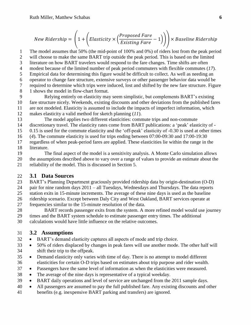
The Excel-based model analyzes existing ridership patterns for a weekday in 15-minute 40

increments. The main calculation determines the ridership under the new fare structure. This uses 41

a rearrangement of the normal elasticity of demand equation: 42


The model assumes that 50% (the mid-point of 100% and 0%) of riders lost from the peak period 1

will choose to make the same BART trip outside the peak period. This is based on the limited 2

literature on how BART travelers would respond to the fare changes. Time shifts are often 3

modest because of the limited number of peak period commuters with flexible commutes (17). 4

Empirical data for determining this figure would be difficult to collect. As well as needing an 5

operator to change fare structure, extensive surveys or other passenger behavior data would be 6

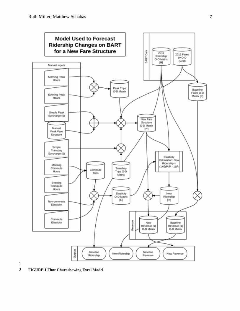
required to determine which trips were induced, lost and shifted by the new fare structure. Figure 7

1 shows the model in flow-chart format. 8

Relying entirely on elasticity may seem simplistic, but complements BART’s existing 9

fare structure nicely. Weekends, existing discounts and other deviations from the published fares 10

are not modeled. Elasticity is assumed to include the impacts of imperfect information, which 11

makes elasticity a valid method for sketch planning (11). 12

The model applies two different elasticities: commute trips and non-commute 13

discretionary travel. The elasticity rates come from BART publications: a ‘peak’ elasticity of -14

0.15 is used for the commute elasticity and the ‘off-peak’ elasticity of -0.30 is used at other times 15

(4). The commute elasticity is used for trips ending between 07:00-09:30 and 17:00-19:30 16

regardless of when peak-period fares are applied. These elasticities lie within the range in the 17

literature. 18

The final aspect of the model is a sensitivity analysis. A Monte Carlo simulation allows 19

the assumptions described above to vary over a range of values to provide an estimate about the 20

reliability of the model. This is discussed in Section 5. 21

3.1 Data Sources 22

BART’s Planning Department graciously provided ridership data by origin-destination (O-D) 23

pair for nine random days 2011 – all Tuesdays, Wednesdays and Thursdays. The data reports 24

station exits in 15-minute increments. The average of these nine days is used as the baseline 25

ridership scenario. Except between Daly City and West Oakland, BART services operate at 26

frequencies similar to the 15-minute resolution of the data. 27

BART records passenger exits from the system. A more refined model would use journey 28

times and the BART system schedule to estimate passenger entry times. The additional 29

calculations would have little influence on the relative outcomes. 30

3.2 Assumptions 31

BART’s demand elasticity captures all aspects of mode and trip choice. 32

50% of riders displaced by changes in peak fares will use another mode. The other half will 33

shift their trip to the offpeak. 34

Demand elasticity only varies with time of day. There is no attempt to model different 35

elasticities for certain O-D trips based on estimates about trip purpose and rider wealth. 36

Passengers have the same level of information as when the elasticities were measured. 37

The average of the nine days is representative of a typical weekday. 38

BART daily operations and level of service are unchanged from the 2011 sample days. 39

All passengers are assumed to pay the full published fare. Any existing discounts and other 40

benefits (e.g. inexpensive BART parking and transfers) are ignored. 41


1

FIGURE 1 Flow Chart showing Excel Model 2


3.3 Limitations 1

The model assumes that all trips in the peak period have an elasticity typical for a suburban 2

rail commuter. 3

The model takes a blunt approach to reassigning riders lost due to fare increases. Without 4

clear guidance from the literature, the decision to split the riders evenly is a helpful 5

approximation. 6

In some cases, a rider may choose to enter or exit from another station to avoid the new fares. 7

The model does not account for shifts in origin or destination when a trip is still taken by 8

BART. 9

The ridership data only records station exits. The model assumes anybody who exits after the 10

peak period will have entered after the peak period, which is untrue for some longer trips. 11

The trip distribution is unchanged from the baseline case. There is no attempt to capture 12

future land use changes, BART extensions, or external factors influencing the decision to use 13

BART. 14

The model only considers weekday trips. When subsidies are given to off-peak trips for a 15

revenue-neutral outcome, these off-peak trips do not include weekends. 16

3.4 Chosen Fare Structures 17

This study modeled five alternative scenarios based on the case studies and two suggested in 18

BART’s 2010 Demand Management Study: 19

Complex – $1 surcharges on both peak period and peak direction (based on London) 20

Peak-Period – 50¢ surcharges on only peak period travel (Washington, D.C.) 21

Narrow Morning Peak - $2 surcharge on trips from 08:00-09:00 22

Station-Based Surcharges - $2.95 surcharge on entries and exits from BART’s busiest 23

stations, Embarcadero and Montgomery, between 08:00-09:00 and 17:00-18:00 24

Flat Fares – Every trip is priced flat at the system average of $3.51 (Toronto) 25

Low Flat Fares – Flat fares artificially lowered to $2.25 (New York) 26

Zones – Applying a new zone map, trips cost $1.75 plus 50¢ for each additional zone 27

(Portland) 28

For each case, a revenue-neutral scenario is included. All additional revenue is applied directly to 29

subsidize off-peak trips. Discounting like this is used extensively around the world to smooth 30

peaks and improve efficiency (8). 31

4 RESULTS AND ANALYSIS 32

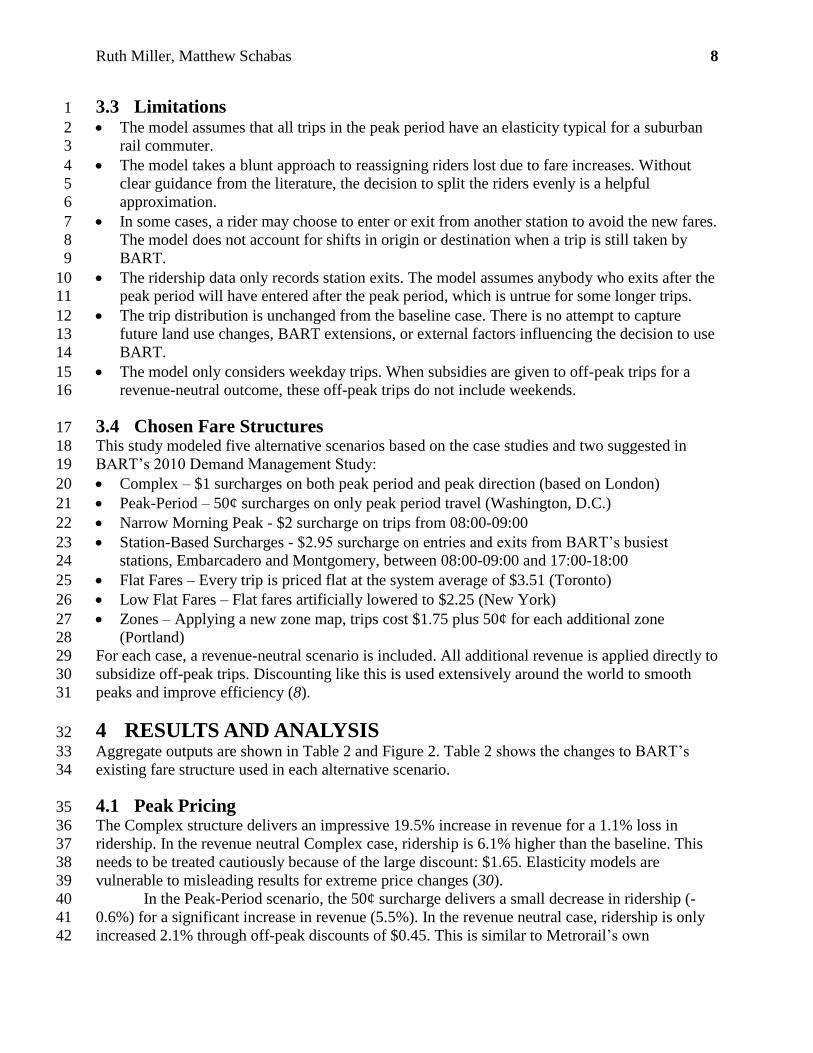
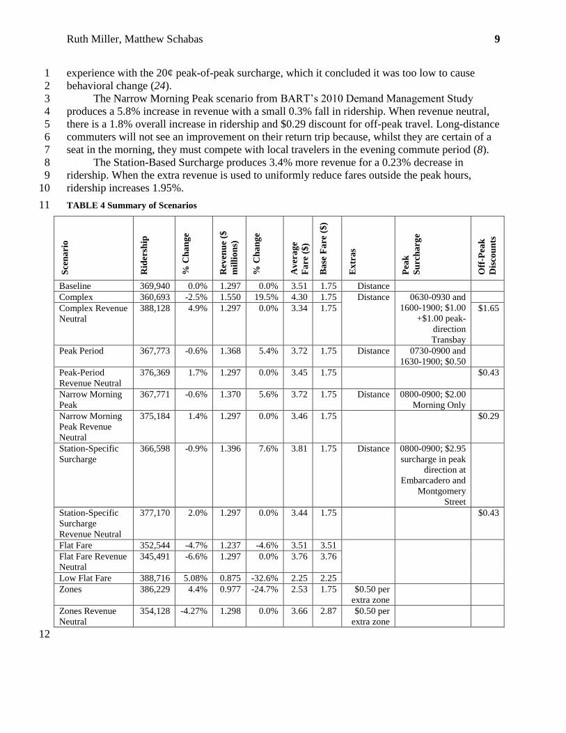
Aggregate outputs are shown in Table 2 and Figure 2. Table 2 shows the changes to BART’s 33

existing fare structure used in each alternative scenario. 34

4.1 Peak Pricing 35

The Complex structure delivers an impressive 19.5% increase in revenue for a 1.1% loss in 36

ridership. In the revenue neutral Complex case, ridership is 6.1% higher than the baseline. This 37

needs to be treated cautiously because of the large discount: $1.65. Elasticity models are 38

vulnerable to misleading results for extreme price changes (30). 39

In the Peak-Period scenario, the 50¢ surcharge delivers a small decrease in ridership (-40

0.6%) for a significant increase in revenue (5.5%). In the revenue neutral case, ridership is only 41

increased 2.1% through off-peak discounts of $0.45. This is similar to Metrorail’s own 42


experience with the 20¢ peak-of-peak surcharge, which it concluded it was too low to cause 1

behavioral change (24). 2

The Narrow Morning Peak scenario from BART’s 2010 Demand Management Study 3

produces a 5.8% increase in revenue with a small 0.3% fall in ridership. When revenue neutral, 4

there is a 1.8% overall increase in ridership and $0.29 discount for off-peak travel. Long-distance 5

commuters will not see an improvement on their return trip because, whilst they are certain of a 6

seat in the morning, they must compete with local travelers in the evening commute period (8). 7

The Station-Based Surcharge produces 3.4% more revenue for a 0.23% decrease in 8

ridership. When the extra revenue is used to uniformly reduce fares outside the peak hours, 9

ridership increases 1.95%. 10

TABLE 4 Summary of Scenarios 11

Sce

na

rio

Rid

ersh

ip

% C

ha

ng

e

Rev

enu

e ($

mil

lio

ns)

% C

ha

ng

e

Av

era

ge

Fa

re (

$)

Ba

se F

are

($

)

Ex

tra

s

Pea

k

Su

rch

arg

e

Off

-Pea

k

Dis

cou

nts

Baseline 369,940 0.0% 1.297 0.0% 3.51 1.75 Distance

Complex 360,693 -2.5% 1.550 19.5% 4.30 1.75 Distance 0630-0930 and

1600-1900; $1.00

+$1.00 peak-

direction

Transbay

Complex Revenue

Neutral

388,128 4.9% 1.297 0.0% 3.34 1.75 $1.65

Peak Period 367,773 -0.6% 1.368 5.4% 3.72 1.75 Distance 0730-0900 and

1630-1900; $0.50

Peak-Period

Revenue Neutral

376,369 1.7% 1.297 0.0% 3.45 1.75 $0.43

Narrow Morning

Peak

367,771 -0.6% 1.370 5.6% 3.72 1.75 Distance 0800-0900; $2.00

Morning Only

Narrow Morning

Peak Revenue

Neutral

375,184 1.4% 1.297 0.0% 3.46 1.75 $0.29

Station-Specific

Surcharge

366,598 -0.9% 1.396 7.6% 3.81 1.75 Distance 0800-0900; $2.95

surcharge in peak

direction at

Embarcadero and

Montgomery

Street

Station-Specific

Surcharge

Revenue Neutral

377,170 2.0% 1.297 0.0% 3.44 1.75 $0.43

Flat Fare 352,544 -4.7% 1.237 -4.6% 3.51 3.51

Flat Fare Revenue

Neutral

345,491 -6.6% 1.297 0.0% 3.76 3.76

Low Flat Fare 388,716 5.08% 0.875 -32.6% 2.25 2.25

Zones 386,229 4.4% 0.977 -24.7% 2.53 1.75 $0.50 per

extra zone

Zones Revenue

Neutral

354,128 -4.27% 1.298 0.0% 3.66 2.87 $0.50 per

extra zone

12


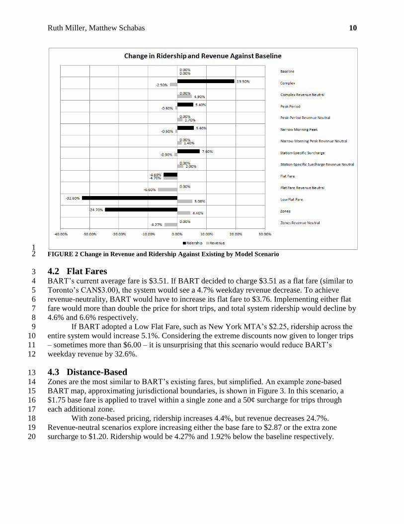
1 FIGURE 2 Change in Revenue and Ridership Against Existing by Model Scenario 2

4.2 Flat Fares 3

BART’s current average fare is $3.51. If BART decided to charge $3.51 as a flat fare (similar to 4

Toronto’s CAN$3.00), the system would see a 4.7% weekday revenue decrease. To achieve 5

revenue-neutrality, BART would have to increase its flat fare to $3.76. Implementing either flat 6

fare would more than double the price for short trips, and total system ridership would decline by 7

4.6% and 6.6% respectively. 8

If BART adopted a Low Flat Fare, such as New York MTA’s $2.25, ridership across the 9

entire system would increase 5.1%. Considering the extreme discounts now given to longer trips 10

– sometimes more than $6.00 – it is unsurprising that this scenario would reduce BART’s 11

weekday revenue by 32.6%. 12

4.3 Distance-Based 13

Zones are the most similar to BART’s existing fares, but simplified. An example zone-based 14

BART map, approximating jurisdictional boundaries, is shown in Figure 3. In this scenario, a 15

$1.75 base fare is applied to travel within a single zone and a 50¢ surcharge for trips through 16

each additional zone. 17

With zone-based pricing, ridership increases 4.4%, but revenue decreases 24.7%. 18

Revenue-neutral scenarios explore increasing either the base fare to $2.87 or the extra zone 19

surcharge to $1.20. Ridership would be 4.27% and 1.92% below the baseline respectively. 20


FIGURE 3 Potential travel zones for BART 1

5 SENSITIVITY ANALYSIS 2

To determine if these assumptions are reasonable, the forecast ridership and revenue were 3

modeled through a Monte Carlo simulation (except the revenue neutral cases, which is beyond 4

the capability of this model). The results are summarized in Table 2 and Table 3. 5

TABLE 2 Monte Carlo Simulation Parameters 6

Variable Minimum Base value used in the Model Maximum

Non-Commute Elasticity -0.1 (14) -0.30 (4) -0.79 (10)

Commute Elasticity -0.09 (13) -0.15 (4) -0.31 (16)

Percent who shift from

Peak to Off-Peak

0% 50% 100%

Morning Commute Period 06:00 07:00 09:30 10:00

Evening Commute Period 16:00 17:00 19:30 20:00

7

The Monte Carlo Simulation suggests that the variables chosen in the model are robust. The 8

model produces values for a sample of alternatives that are within one standard deviation of the 9

mean of the 1,000 iteration Monte Carlo Simulation, concluding that the results of the sketch-10

planning model appear believable and that the assumptions are reasonable. 11


TABLE 3 Monte Carlo Simulation Summary 1

Scenario Weekday Revenue ($ millions) Weekday Ridership

Mo

del

Mo

nte

Ca

rlo

Mea

n

Sta

nd

ard

Dev

iati

on

Ch

an

ge

from

Mo

del

Mo

del

Mo

nte

Ca

rlo

Mea

n

Sta

nd

ard

Dev

iati

on

Ch

an

ge

from

Mo

del

Baseline 1.297 n/a n/a n/a 369,940 n/a n/a n/a

Complex 1.550 1.535 0.032 -0.015 360,693 358,386 7,809 -2,307

Peak-

Period

1.368 1.365 0.007 -0.003 367,773 366,911 2,089 -862

Narrow

Morning

Peak

1.370 1.363 0.011 -0.007 367,771 366,829 2,401 -942

Flat Fare 1.237 1.217 0.028 -0.020 352,544 346,681 8,081 5,863

Low Flat

Fare

0.875 0.891 0.019 0.016 388,716 395,876 8,628 7,160

6 DISCUSSION OF RESULTS 2

This discussion is restricted to the impact of different fare structures on ridership and revenue. 3

Qualitative equity considerations are discussed in section 6.3. 4

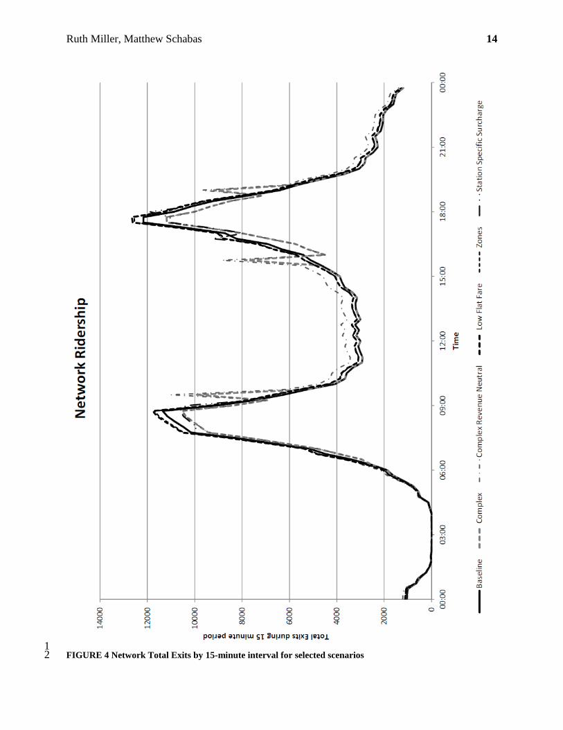
6.1 Ridership 5

Ridership is a standard measure of performance for public transit. BART currently – and in all 6

the scenarios – mainly serves commute travel in the morning and evening peaks – see Figure 4. 7

There is ample off-peak capacity. 8

6.1.1 Total Daily Ridership 9

The model methodology assumes off-peak fare discounts result in ridership increases. Fare 10

structures that generally reduced fares increased ridership. The Low Flat Fare and Zones 11

scenarios substantially reduce the cost of longer trips, and encourage many more people to ride 12

BART (5.1% and 4.4%, respectively). The cost of using Zones is a 24.7% fall in revenue. All 13

scenarios with peak surcharges reduced overall ridership. 14

For revenue-neutral cases, the Complex scenario produced the highest ridership increase 15

over the base case (4.9%); followed by the other peak surcharge scenarios. The revenue neutral 16

cases show that it is possible to increase ridership without losing revenue. 17

The model shows that even major discounting will not increase total system ridership as 18

much as introducing a complex peak fare structure and using the extra revenue to heavily 19

discount off-peak travel. Simple fare structures, such as Flat Fare and Zones, actually decrease 20

ridership if something close to the current average fare is maintained. 21

6.1.2 Congestion Management 22

BART is concerned about congestion at Embarcadero and Montgomery Street stations in 23

downtown San Francisco (4). Effective congestion management shifts riders to less congested 24

times. As it maximizes riders within existing capacity, congestion management is a more refined 25

goal than ridership. One measure for the proposed scenarios is how much they smooth the peak 26


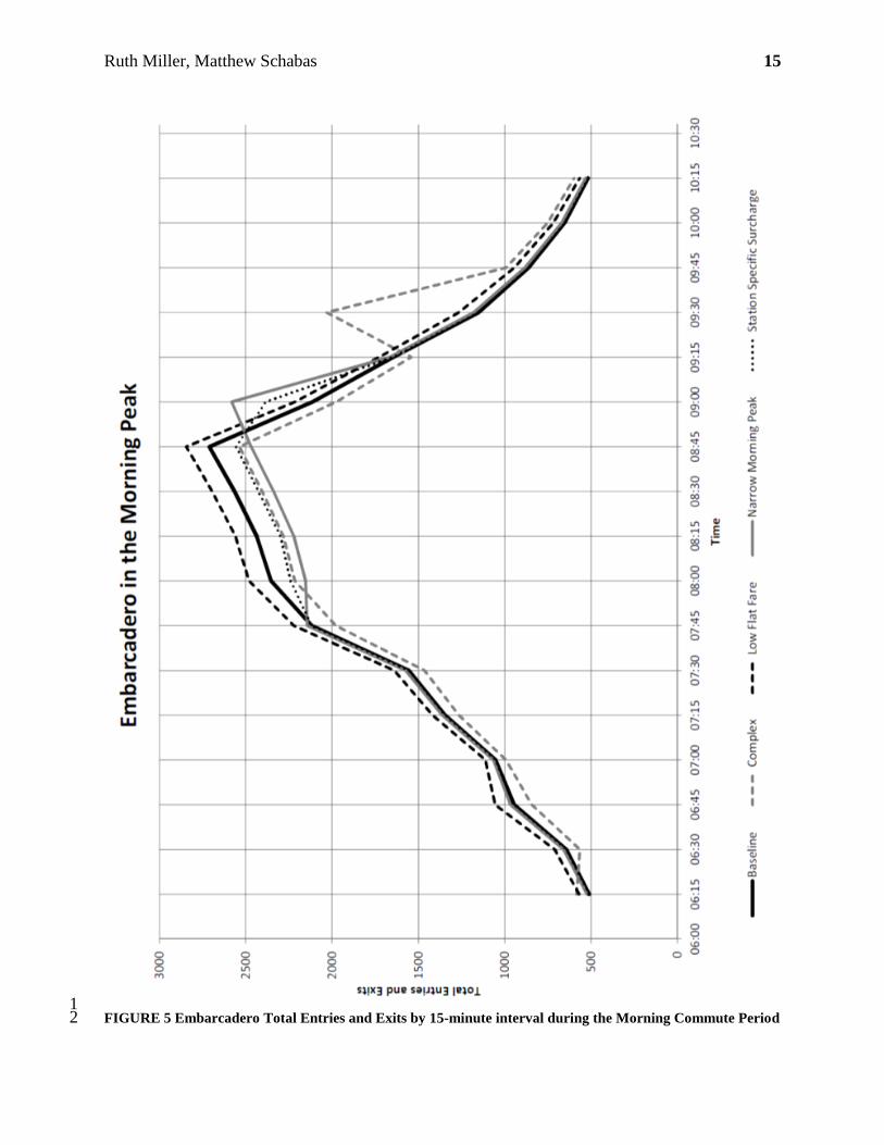
at Embarcadero and Montgomery Street stations. Figure 5 shows the passenger volume at 1

Embarcadero during the morning peak for selected fare structures. 2

Peak pricing – in any form – has great potential to lower the high passenger volumes, 3

although the model still projects ridership exceeding the station capacity of 2,500 passengers per 4

15-minute interval. 5

The spikes at 09:00 and 09:30 for the Complex Revenue Neutral and Narrow Morning 6

Peak revenue neutral are produced by the model’s simple reallocation of lost riders to the off-7

peak period. This effect is to be expected, and can be observed on the peak-priced Bay Bridge 8

nearby, though the magnitude of such an effect is difficult to estimate. 9

Fares influence travel behavior, and can create congestion as easily as managing it. The 10

two flat fare scenarios show that some pricing structures can make peak periods more congested. 11

BART’s existing fare policy already avoids this worst-case scenario, but the success of the other 12

scenarios suggests BART could do more to relieve congestion. 13

Figure 4 reveals an important point about how the different scenarios increase ridership. 14

Low Flat Fare and Zones gain riders during the peak with small off-peak gains. The Complex 15

revenue neutral case reduces peak loading and gains riders during the off-peak period. 16

6.2 Revenue 17

The Complex fare is the overwhelming winner for revenue generation, increasing weekday 18

revenue by 19.5%. This would improve farebox recovery to an impressive 86% (22). Other 19

revenue-favorable scenarios include the Station-Specific Surcharge (7.6%), Narrow Morning 20

Peak (5.6%), and Peak-Period (5.4%). All of these systems introduce a new level of specificity to 21

BART’s existing fare structure, either by time or station. 22

In all peak surcharge scenarios, the lost riders will be in the congested commute period. 23

Losing riders relative to the baseline may actually be desirable. BART is concerned about 24

capacity constraints at Embarcadero and Montgomery Street Station and crowding on trains 25

using the TransBay Tube (4). 26

In every case, simpler structures decrease revenue. The Low Flat Fare and Zones 27

decrease revenue significantly (-32.6% and -24.7%, respectively), while Flat Fares manage to 28

lose both revenue (4.6%) and ridership. 29


1 FIGURE 4 Network Total Exits by 15-minute interval for selected scenarios 2


1 FIGURE 5 Embarcadero Total Entries and Exits by 15-minute interval during the Morning Commute Period 2


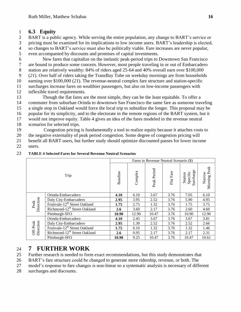
6.3 Equity 1

BART is a public agency. While serving the entire population, any change to BART’s service or 2

pricing must be examined for its implications to low income users. BART’s leadership is elected, 3

so changes to BART’s service must also be politically viable. Fare increases are never popular, 4

even accompanied by discounts and promises of capital investments. 5

New fares that capitalize on the inelastic peak-period trips to Downtown San Francisco 6

are bound to produce some concern. However, most people traveling in or out of Embarcadero 7

station are relatively wealthy: 84% of riders aged 25-64 and 40% overall earn over $100,000 8

(21). Over half of riders taking the TransBay Tube on weekday mornings are from households 9

earning over $100,000 (21). The revenue-neutral complex fare structure and station-specific 10

surcharges increase fares on wealthier passengers, but also on low-income passengers with 11

inflexible travel requirements. 12

Though the flat fares are the most simple, they can be the least equitable. To offer a 13

commuter from suburban Orinda to downtown San Francisco the same fare as someone traveling 14

a single stop in Oakland would force the local trip to subsidize the longer. This proposal may be 15

popular for its simplicity, and to the electorate in the remote regions of the BART system, but it 16

would not improve equity. Table 4 gives an idea of the fares modeled in the revenue neutral 17

scenarios for selected trips. 18

Congestion pricing is fundamentally a tool to realize equity because it attaches costs to 19

the negative externality of peak period congestion. Some degree of congestion pricing will 20

benefit all BART users, but further study should optimize discounted passes for lower income 21

users. 22

TABLE 4 Selected Fares for Several Revenue Neutral Scenarios 23

Trip

Fares in Revenue Neutral Scenario ($)

Bas

elin

e

Co

mp

lex

Pea

k P

erio

d

Fla

t F

are

Sta

tio

n

Sp

ecif

ic

Su

rch

arg

e

Nar

row

Mo

rnin

g P

eak

Pea

k

Dir

ecti

on

Orinda-Embarcadero 4.10 6.10 3.67 3.76 7.05 6.10

Daly City-Embarcadero 2.95 3.95 2.52 3.76 5.90 4.95

Fruitvale-12th

Street Oakland 1.75 2.75 1.32 3.76 1.75 3.75

Richmond-12th

Street Oakland 2.6 3.60 2.17 3.76 2.60 4.60

Pittsburgh-SFO 10.90 12.90 10.47 3.76 10.90 12.90

Off

-Pea

k

Dir

ecti

on

Orinda-Embarcadero 4.10 2.45 3.67 3.76 3.67 3.81

Daly City-Embarcadero 2.95 1.30 2.52 3.76 2.52 2.66

Fruitvale-12th

Street Oakland 1.75 0.10 1.32 3.76 1.32 1.46

Richmond-12th

Street Oakland 2.6 0.95 2.17 3.76 2.17 2.31

Pittsburgh-SFO 10.90 9.25 10.47 3.76 10.47 10.61

7 FURTHER WORK 24

Further research is needed to form exact recommendations, but this study demonstrates that 25

BART’s fare structure could be changed to generate more ridership, revenue, or both. The 26

model’s response to fare changes is non-linear so a systematic analysis is necessary of different 27

surcharges and discounts. 28


The dataset used in this report makes any equity or environmental analysis a large 1

extension of the available facts. Analysis is needed to consider the consequences of a new fare 2

structure. The model implemented here is not designed for this. Consideration of what modes 3

BART would be competing with is important for both. If fare changes shift passengers for short 4

trips to bikes and walking then there may be few negative consequences. If increases come at the 5

expense of long distance car commutes then the changes may be very important. 6

8 CONCLUSIONS 7

The model suggests that BART has an opportunity to increase ridership and revenue whilst 8

mitigating congestion through more complex fare strategies. A good fare policy will increase 9

ridership in off-peak periods, increase revenue, provide equity to riders, and support larger plans 10

to meet environmental goals. 11

A scenario with peak periods and peak direction surcharges increases BART’s weekday 12

revenue by 19.5%, providing funds that could reduce off-peak fares and fund modernization. A 13

revenue-neutral version of this scenario increases BART’s weekday ridership by 4.9%. 14

BART is facing unfunded deferred maintenance and needs new rolling stock. Finding 15

ways to raise revenue from fares may make state and ballot measure funding politically 16

acceptable because users are helping pay for improvements. Public transit offers essential 17

mobility for low income groups. Like many suburban rail networks, BART’s ridership has 18

disproportionately high household incomes so increasing fares on inelastic commuter travel, 19

though unpopular, may not be inequitable. 20

BART already has the technology for collecting more complex fares. Implementing 21

complex fares may be a way to improve BART’s value-for-money to both the regional taxpayer 22

– through higher revenue – and its customers – with less congestion and cheaper off-peak travel 23

– without major capital expenditure. 24

9 WORKS CITED 25

1. Deakin, E., G. Tal, and K. Frick. What Makes Public Transit a Success? Perspectives on

Ridership in an Era of Uncertain Revenues and Climate Change. in TRB 2010 Annual

Meeting CD-ROM, 2010.

2. Deakin, E., A. Reno, J. Rubin, S. Randolph, and M. Cunningham. BART State of Good

Repair Report. Transform, Nov. 04, 2011. http://transformca.org/files/

bart_sogr_regional_impacts_2011-11-04.pdf.

3. BART. Short Range Transit Plan (FY08 through FY17) and Capital Improvement Program

(FY08 through FY32). 2007.

4. Nelson Nygaard. BART Demand Management Study. 2010.

5. Cervero, R. Flat Versus Differentiated Transit Pricing: What's a Fair Fare? Transportation,

1981, pp. 211-232.

6. Grey, A., and D. Lewis. Public Transport Fares and the Public Interest. The Town Planning

Review, July 1975, pp. 295-313.

7. Hale, C., and P. Charles. Practice Reviews in Peak Period Rail Network Management:

Sydney & San Francisco Bay Area. 2009.

8. Henn, L., G. Karpouzis, and K. Sloan. A review of policy and economic instruments for peak

demand management in commuter rail. in The 33rd Australasian Transport Research Forum


Conference, 2010.

9. Hensher, D. A. Establishing a Fare Elasticity Regime for Urban Passenger Transport. Journal

of Transport Economics and Policy, May 1998, pp. 221-246.

10. Paulley, N., R. Balcombe, R. Mackett, H. Titheridge, and J. Preston. The demand for public

transport: The effects of fares, quality of service, income and car ownership. Transport

Policy, no. 13, 2006, pp. 295–306.

11. de Rus, G. Public Transport Demand Elasticities in Spain. Journal of Transport Economics

and Policy, Vol. 24, No. 2, 1990, pp. 189-201.

12. Mezghani, M. Study on electronic ticketing in public transport. 2008.

13. Pratt, R. H. Traveler Response to Transportation System Changes. 2000.

14. Litman, T. Transit Price Elasticities and Cross-Elasticities. Journal of Public Transportation,

Vol. 7, no. 2, 2011, pp. 37-58, Update to 2004 paper (Victoria Transport Policy Institute):

http://www.vtpi.org/tranelas.pdf. http://www.vtpi.org/tranelas.pdf.

15. TCRP. Transit Pricing and Fares. Transit Cooperative Research Program, Vol. 95, 2004, pp.

1-58.

16. Reinke, D. Recent Changes in BART Patronage. Washington, DC, 1988.

17. Cervero, R. Transit Pricing Research: A review and synthesis. Transportation 17, 1990, pp.

117-139.

18. Nuworsoo, C., A. Golub, and E. Deakin. Analyzing equity impacts of transit fare changes:

Case study of Alameda–Contra Costa Transit, California. Evaluation and Program Planning

32, 2009, pp. 360-368.

19. Santos, G., and G. Fraser. Road Pricing: Lessons from London. 2005.

20. Evans, R. Demand Elasticities for Car Trips to Central London as revealed by the Central

London Congestion Charging Zone. 2008.

21. BART. 2008 Station Profile Report. 2008.

22. APTA. T26 2010 Pass Fare Recovery Ratio. American Public Transportation Association,

2012. http://www.apta.com/resources/statistics/Documents/NTD_Data/2010_NTD/

T26_2010_Pass_Fare_Recovery_Ratio.xls. Accessed April 09, 2012.

23. TfL. Tube, DLR and London Overground Fares, 2012. http://www.tfl.gov.uk/tickets/

14416.aspx.

24. Smith, M. Public Transit and the Time-Based Fare Structure. Chicago, 2009.

25. WMATA. Metrorail Fares. WMATA, 2012. http://www.wmata.com/fares/metrorail.cfm.

Accessed April 10, 2012.

26. TTC. TTC Fare Collection Study. 2000.

27. TTC. 2010 Annual Report. 2011.

28. New York MTA. Fares and Metrocard. 2012. http://www.mta.info/metrocard/mcgtreng.htm.

29. Tri-Met. Tri-Met Rail System. Tri-Met, 2012a. http://trimet.org/maps/railsystem.htm.

30. Goodwin, P. B., and H. C.W.L. Williams. Public Transport Demand Models and Elasticity

Measures: An Overview of Recent British Experience. Transportation Research Board vol.

19B, 1985, pp. 253-259.

1

Date post:	20-Jan-2017
Category:	Documents
Upload:	ruth-miller
View:	109 times
Download:	0 times