Alumni Scoring System of Worcester Polytechnic Institute’s Alumni Database A Major Qualifying Project Report Submitted of the Faculty of the WORCESTER POLYTECHNIC INSTITUTE in partial fulfillment of the requirements for the Degree of Bachelor of Science by ___________________________________ Kirsten B. Murphy ___________________________________ Onalie L. Sotak Date: APRIL 26, 2007 Approved: _______________________________________ Professor Arthur C. Heinricher, Advisor ______________________________________ Professor Jon P. Abraham, Advisor _______________________________________ Professor Jayson D. Wilbur, Advisor
Transcript
Alumni Scoring System
of Worcester Polytechnic Institute’s Alumni Database
A Major Qualifying Project Report
Submitted of the Faculty
of the
WORCESTER POLYTECHNIC INSTITUTE
in partial fulfillment of the requirements for the
Degree of Bachelor of Science
by
___________________________________
Kirsten B. Murphy
___________________________________
Onalie L. Sotak
Date: APRIL 26, 2007
Approved:
_______________________________________
Professor Arthur C. Heinricher, Advisor
______________________________________
Professor Jon P. Abraham, Advisor
_______________________________________
Professor Jayson D. Wilbur, Advisor
ii
Abstract
The primary goal of this project was to construct and evaluate a scoring method for
ranking individuals in a database where those more likely to donate receive higher scores.
The created spreadsheet takes donor information and generates an assigned score from 1-
20. A manual for the spreadsheet was also created, enabling the WPI Office of
Development and Alumni Relations to rank selected alumni in order of their likelihood to
donate in the future.
iii
Acknowledgments
We would first like to start by thanking our three advisors Professors Arthur
Heinricher, Jon Abraham, and Jayson Wilbur for their support, guidance, and tremendous
patience with us throughout this year. The different insights provided throughout the
project created a challenging, yet overall rewarding experience and we appreciate their
continued effort to educate and push us to succeed.
We would like to give a huge thanks to the WPI Office of Development and
Alumni Relations for providing assistance and access to the data used in this project. We
would especially like to thank Dexter Bailey (Vice President for WPI Office of
Development and Alumni Relations) and Lisa Maizite (Assistant Vice President for WPI
Office of Development and Alumni Relations) for their cooperation, trust, and continued
sincere interest throughout this project was helpful as well as rewarding.
We would like to thank Professor Bogdan Vernescu for initially identifying this
project opportunity for us. Huge thanks also go to Yi “Danny” Jin for his work on this
database and assistance in answering questions and guidance and conclusions that were
used as a basis for a majority of this project. While not in direct contact with us during
this project, Professor Joseph Petruccelli provided guidance for Jin and we would like to
thank him for his previous work as well as his availability to us during the project if we
had needed additional assistance.
We lastly would like to thank our friends and family who supported us throughout
the project and provided both insight and comfort during this year.
iv
Table of Contents
Abstract ............................................................................................................................... ii Acknowledgments.............................................................................................................. iii 1. Introduction..................................................................................................................... 1 2. Background..................................................................................................................... 3
2.1 Data Mining .............................................................................................................. 4 2.2 Scoring System ......................................................................................................... 5 2.3. Summary................................................................................................................ 13
3. Exploring the Data ........................................................................................................ 15 3.1 Focus Population..................................................................................................... 18 3.2 Removing Outliers in Alumni Database................................................................. 19 3.3 Alumni-only Database Summary............................................................................ 20
3.3.1 Variable Types ................................................................................................. 20 3.4 Analysis of Donations per Fiscal Year 1983-2007................................................. 28
3.4.1 Associations between Variables ...................................................................... 30 3.5 Conclusion .............................................................................................................. 32
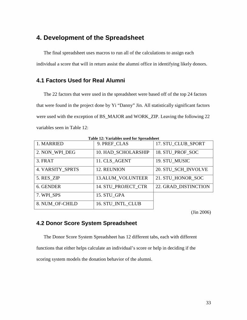
4. Development of the Spreadsheet .................................................................................. 33 4.1 Factors Used for Real Alumni ................................................................................ 33 4.2 Donor Score System Spreadsheet ........................................................................... 33
5.1 Determining the Score Factors................................................................................ 41 5.2 Metric System ......................................................................................................... 43 5.3 Graph Results.......................................................................................................... 44
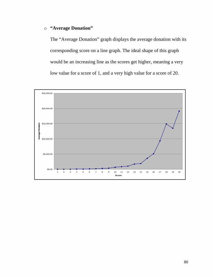
5.3.1 Number of Individuals in each Score Bucket .................................................. 44 5.3.2 Total Donated................................................................................................... 45 5.3.3 Average Donation ............................................................................................ 46 5.3.4 Percent Donating.............................................................................................. 47
5.4 Summary................................................................................................................. 48 6. Conclusions............................................................................................................... 49 Appendix A: Donation Behavior of Blank and Non-Blank Variables ............................. 53 Appendix B: Donation Behavior of Individual States ...................................................... 55 Appendix C: Donation Behavior of Massachusetts Region ............................................. 57 Appendix D: Average and Median Donation by Fiscal Year 1983 to 2007..................... 58 Appendix E: Percent of People Donating by Fiscal Year 1983 to 2007........................... 59 Appendix F: Total Donations by Fiscal Year .................................................................. 60
v
Appendix G: Score Factors for Zip Code Ranges ............................................................ 61 Appendix H: User’s Manual provided for Donor Score System ...................................... 65
vi
Table of Figures
Figure 1: Actual and Inflation Adjusted Donations......................................................... 30 Figure 2: Total People for each Score............................................................................... 45 Figure 3: Total Donated for each Score............................................................................ 46 Figure 4: Average Donation for each Score ..................................................................... 47 Figure 5: Percentage Donating for each Score ................................................................. 48
vii
Table of Tables
Table 1: Distribution of Donation Size by E-Mail Variable.............................................10 Table 2: Distribution of Donation Size by Marital Status Variable.................................. 10 Table 3: Modified Data Extract Key................................................................................. 16 Table 4: Donation Behavior by Fraternity Variable ......................................................... 22 Table 5: Donation Behavior by Marital Status Variable .................................................. 24 Table 6: Donation Behavior by Gender Variable ............................................................. 25 Table 7: Donation Behavior by Bachelor’s Degree Variable ........................................... 26 Table 8: Donation Behavior of GPA Variable.................................................................. 27 Table 9: Donation Behavior of Graduate Classes by Decade........................................... 28 Table 10: Donation Behavior by Gender and Graduation Year ....................................... 31 Table 11: Donation Behavior by Marital Status and Graduation Year............................. 31 Table 12: Variables used for Spreadsheet......................................................................... 33 Table 13: Statistics for FRAT variable ............................................................................. 41 Table 14: Score Factors used for Blank/Non-Blank Variables......................................... 42 Table 15: Score Factors used for MARRIED, GENDER and PREF_CLAS ................... 42 Table 16: Metric Values for Final Score System.............................................................. 44 Table 17: Metric Sums for Final Score System................................................................ 44
1
1. Introduction Universities spend time and money to collect and organize alumni information
and this project aims to reward WPI for its effort in this area. Alumni, as well as friends
and family of alumni, are an important source of support for the university, both
financially and non-financially. The cost is increased by the task of contacting alumni for
donations. While this project focuses specifically on fundraising at an academic
institution, this is a problem for any organization that tries to identify likely donators.
This project uses information in the WPI donor database to rank each individual’s
likelihood of donating. The goal of this project was to build a scoring algorithm to
identify likely donors and implement that algorithm in a software application that the
WPI Office of Development and Alumni Relations can use to prioritize individuals for
fundraising activities.
A spreadsheet was created to implement the Donor Score System that could
measure an individual’s likelihood of donating based on a variety of factors provided in
the database that coincide with past donation trends. Advances in technology have made
it possible to store and update massive amounts of records easily. More data does not
mean more information. Statistical analysis of a dataset builds models that “fit” the data
and provide information about the data, and a scoring system allows for the organization
of information drawn from a dataset by ranking alumnus. This score is determined from
the information provided in the WPI database and the individual scores that are assigned
to different recorded information about an individual. Once the donor score system
identifies a person as likely to donate, it then assigns that individual a score from 1 to 20.
2
With this score, the program produces a list of ranked individuals in the database and
provides their contact information.
A manual for the spreadsheet was created and was provided to the Alumni Office
with instructions for using the donor score system. This manual explains how the
spreadsheet works and how it provides a quick and effective means of organizing the
database to produce the best prospects to contact first. The donor scoring system
provides the WPI Office of Development and Alumni Relations with more time to focus
on alumni events and less time sorting through unorganized information or blindly calling
alumni with little to no likelihood of donating. With near 25,000 alumni worldwide, WPI
can use the donor score system and mine its database information, in order to reduce
costs spent on finding and contacting alumnus, and increase donations by using the
Donor Score System to efficiently identifying and in turn contacting those records in the
database who are more likely to donate.
3
2. Background
This project goal is to extract information from a large data set and use it to help
identify donors. Sampling is a method commonly used as a way to reduce the size of a
dataset to obtain a manageable and representative set of data. Analysis of the original
large datasets relies heavily on computational power, and this type of power is now
available to aid in statistical analysis and statistical modeling of data. Computers and
software are the tools used to explore large data sets. Statistical analysis usually assumes
that variables in a dataset are related in some mathematical way and statistical tools can
find these relationships. For example a person’s age and lifestyle can be used to predict
mortality, and similarly the same type of characteristics can be used to predict donation
activity.
Another WPI student, Yi Jin, analyzed the WPI database to identify 24 variables
that were related to donation behavior (Jin 2006). His analysis assumed that donation
behavior is a function of factors in the database. The following equation 2.1 is a linear
regression model with p predictors:
∑=
++=p
iii XY
10 εββ (2.1)
where Y is the value of the dependent variable, β0 is the intercept, βi is the coefficient for
the i th independent known constant Xi (i = 1, 2, … p) and є is the independent random
error term (Kutner, Nachtsheim, and Neter, 2005). Using equation (2.1) for a set of data
from a donor database, each Xi represents one of the known independent variables in the
database. Each βi would represent the relative affect that variable i has on donation
behavior if all other variables were held constant. While no linear regression was done in
4
this project to determine scores, it was used by Jin to determine the 24 variables that
influence donation behavior the most (Jin 2006).
This project relies more heavily on the scoring system methods similar to those
developed by Peter B. Wylie (2004). This section will introduce data mining; what it is,
what it is used for, and how it relates to this project. It will investigate the scoring
systems created by Wylie as well as a modified score system for use on WPI database.
Finally, it will describe metrics and how they were used in this project to help rate the
scores used in the donor score system.
2.1 Data Mining Data mining relies heavily on computational power and solves problems by
analyzing already present data from databases (Frank 2000). “It [data mining] is not so
much a single technique as the idea that there is more knowledge hidden in the data than
shows itself on the surface” (Adriaans 1996). For this project, the database being
investigated contains information pertaining to WPI’s alumni, as well as family and
friends of alumni.
The database contains 102 variables for 48,604 individuals. A large part of data
mining revolves around not just the access to information but the preparation of the data
being analyzed. “One objective of data preparation is to end with a prepared data set that
is of maximum use for modeling, in which the natural order of the data is least disturbed,
yet that is best enhanced for the particular purposes of the miner” (Pyle 1999). This
quote discusses not only the importance of an organized database, but also the importance
of data cleaning and preparation. Recognizing that there was hidden information in the
database, and then cleaning and preparing the database were introduced through research
5
on data mining and will be discussed in Chapter 3 when a more detailed summary of the
database is discussed.
2.2 Scoring System A technique known as list scoring can be used to rate factors according to their
influence on donation behavior, and a model can be created from this information to rank
the individuals based on their factor values (Wylie 2004). The score assigned to each
factor is guided by patterns in the dataset, and the focus of a score system is to rank
individuals based on their donations, not on predicting the amount of donation made by
an individual. Therefore a score system essentially rearranges and organizes a dataset
based on donation behavior, and list scoring is simply a means of organizing the assigned
scores into list form.
Some factors will have a relationship with donation behavior, some will not.
Wylie identified 3 important factors in his example but some applications may require
more. Once these factors are identified, Wylie used them to create a scoring system. A
score of 0 was given to the portion of the individual variable that didn’t coincide with
positive donation behavior, and a 1 was given to value of the variable that did appear to
coincide with positive donation behavior. For example, Wylie found that individuals
with their e-mail listed donated more than those who did not have their e-mail listed.
Wylie therefore would give anyone with their e-mail listed a score of a 1 and anyone who
left this variable blank would receive a score of 0.
The scores for individual factors are summed to obtain a total score for each
individual in the data set. Wylie’s example uses only 3 variables causing a score of a 0 to
signify that the individual in question does not fit into any of the positive category three
6
factors that Wylie had previously identified as coinciding with positive donation behavior
listed, while a score of a 3 signifies an individual has all three of the factors that Wylie
has previously identified as coinciding with positive donation behavior listed.
With the score system established for the first half of the database, the final step is
to apply the score system on the second half of the data. This step may appear redundant
seeing as Wylie has access to all the information and it would seem that using all the data
when creating the score system would achieve the best conclusions using all available
information. However, Wylie explains that “when you do a project like this, it’s easy to
take advantage of the idiosyncrasies of one sample to generate a scoring
formula/segmentation schema that looks great on that particular sample, but turns out to
be not so great on another sample. We want to see if the relationship between scores and
giving we get in one sample looks as good (or almost as good) on another sample. If it
does, then we can be confident we’re headed in the right direction” (Wylie 2004).
The set of data that is used to create the score system is commonly called the
training data while the second half is called validation or test data. The first half of the
data is used as a training set to fit the model, and the remaining 50% is used to assess
how accurate the model for the first half of the data fits the second half of the data (Hastie,
Friedman, and Tibshirani, 2001). This division of data into two sets is used to help
decide between different models on a set of data. A good model would return similar
results on the second half of the data as were found for the first half of the data. For this
project a good model would not only support the scores for the scoring system, but also
identify that while there may be idiosyncrasies in the data they had no influence in
determining the scores.
7
The model for this project is the scoring system and the scores assigned to
variables are what are determined through the modeling of the first half of a data set and
assessed with the second half of the data set. Sampling is important because “it guides
the choice of learning method or model, and gives us a measure of the quality of the
ultimately chosen model” and discussion of how data was sampled for this project will be
discussed in Chapter 3 (Hastie, Friedman, and Tibshirani, 2001).
To determine important factors Wylie spent a large amount of time organizing
data in the database into charts or graphs to become familiar with the data, and then used
his familiarity with the database to help him decide on important factors. A frequently
asked question in his book revolves around the guidelines for deciding whether or not a
difference between two factors is statistically significant. He explained that when
analyzing a table or graph, if there is something that immediately jumps out, then it
should be studied further in depth to determine its practical significance. He also notes
that the factors chosen were primarily found through intuition, and although his example
only used three variables, there is no restriction on the number of variables that can be
investigated.
Before assigning the individual scores for the variables in the score system, some
exploration of the data needs to be performed to first identify good factors. While a
factor may appear to be highly correlated with donation behavior; donation activity is
extremely sensitive. Sensitivity is due to the occasional large donations made by
individuals through money left in a will or a random philanthropist. With donations
made to universities generally not being millions of dollars, a random million dollar
donation made by a single male mechanical engineer essentially disrupts previous
8
predictions by suddenly identifying any single donators, any male donators, and any
mechanical engineer donators as being extremely likely to donate, when in reality this
may not be the case.
While a good scoring system should assign scores to individuals so that an
individual with a score of a 1 is donating less than an individual with a score of a 2 and so
on, a good score system does not guarantee that the scores will always coincide perfectly
with donation behavior. To test how well a score system fits a set of data, metrics are
used to evaluate the assigned scores for individual factors and ensure that no variables are
incorrectly correlated with donation behavior. While the score system itself determines
how good of a chance there is for an individual to donate based off their factors, metrics
essentially determine how good is the score system itself in assigning the individual
scores.
2.2.1. Donor Score System
The donor score system was set up the same way as Wylie’s system, with the
same objective of assigning scores to records in a database based on their variables. This
section will explore some of the differences between the Wylie system and the donor
system as well as discuss why a scoring method is such an effective means of
determining donation activity. A description of how the score system is used in the Excel
spreadsheet is explained in Chapter 4, and the detailed steps for using the Excel
spreadsheet are explained in the Users Manual in Appendix G.
The principal difference between the score that Wylie’s system assigns and the
score that the donor system assigns lies in the assigning of scores not only to donation
behavior but also relative to other variables in the score system. For example, if Wylie
9
identified being married as having a positive association with donation behavior, and
being a man as correlated with a positive donation behavior, than each married male
would receive a score of 2, and each single female would receive a score of 0. While this
still organizes individual’s donation behaviors based on their marital status and gender,
the donor score system goes an extra step by then investigating how the variables marital
status and gender relate to one another.
If married individuals have a high probability of donating, say someone who is
married donates 100 times more than someone who is single, but men only donate twice
as often as women, then the donor score system takes this into consideration. While it
would still be important to give a male a higher score than a female, it would appear that
a female who was married is actually more likely to donate than a male who was single
because the marital status variable is significantly more influenced by donation behavior
than gender. The donor scoring system allows for a variety of scores, therefore instead of
limiting the score to either a 0 or 1, a smaller score could be assigned for gender and a
larger score could be assigned for marital status.
Another difference lies in the number of variables involved in Wylie’s example,
which only investigated 3 while the donor system contains 24. The quantity of the
variables involved in the system is not as important as the type of variable involved.
Wylie’s 3 variables are “blank or non-blank” variables, while the donor system deals with
both blank and non-blank variables and multiple category variables. Detailed
explanations and examples of both blank and non-blank variables and multiple category
variables will be discussed further in Chapter 3.
10
An example of a table that Wylie provided in his book that illustrates a blank or
non-blank variable, which Wylie refers to as listed or not listed, can be seen in Table 1.
In Table 1 Wylie examined individuals in his database who had provided their e-mail or
had no e-mail listed.
Table 1: Distribution of Donation Size by E-Mail Variable
No E-mail Listed E-Mail Listed Total $0 1,215 523 1,738
$1-$250 1,010 594 1,604 $251 or more 953 705 1,658
Total 3,178 1,822 5,000
He found that approximately one third of the individuals had their e-mail listed and the
remaining did not. Table 1 provides information about e-mail listing by donation size.
While the variable e-mail in Wylie’s example was only investigated based on whether it
was listed or not in the database, the variable marital status in the WPI database was
investigated according to the details of this specific variable, not just simply whether
someone listed their marital status or not. For the donor score system, an example of a
table used to illustrate the marital status variable from the WPI database is in Table 2.
Table 2: Distribution of Donation Size by Marital Status Variable
Married Single Other Blank Total # Of 12,899 10,260 728 140
Total $ Donated $66,289,522.44 $2,728,014.51 $7,203,267.70 $4,641,256.02 Total # Donated 9,929 3,797 604 34 Percent Donated 76.97% 37.01% 82.97% 24.29%
Average Donation $5,139.12 $265.89 $9,894.60 $33,151.83
2.2.2. Metrics
The “Metrics” worksheet is setup to help analyze how accurate the scoring system
is by using three different techniques: the R-Squared method, Sum of Slopes and the
“O.K” method. Each of these techniques has a way of giving a score as to how accurate
11
the current scoring system is using the current factors. The R-squared method determines
how closely the data compares with a best-fit line. The other two methods are there to
compare how increasing the values are. A prefect scoring system when comparing the
average donation with each score bucket should be increasing as the score is increasing.
Meaning that the higher a score a person has, the more likely they are to donate more
money. Using these metrics will hopefully help find the best score factors for each of the
factors that will maximize each of the metrics.
Metric #1 is the R-squared Technique. The R-squared value is a descriptive
measure between 0 and 1. The closer it is to one, the better the model explains the
variation in the data. A value of R-squared equal to one implies that the regression
provides perfect predictions. The formula for R-squared is R2 = 1 – (SSError / SSTotal). This
technique is good to see how much of the donating pattern can be explained by the score
“bucket”.
Metric #2 is the Sum of Slopes Technique used for the Average Donation. This
technique is used to make sure that the function is increasing. It calculates the sum of all
slopes and then divides each slope by the number of people in each of the two associated
score “buckets”, i.e. = 1Σmax – 1 ([(ki+1 – k i)(#k i + #k i+1)]/600). Where ki is the average donated in
the “bucket” where the score is equal to i, and #ki is equal to the number of people that are in this
i th score “bucket”. In the sample population this is finally divided by 300 which is two times the
total number people in the population. The optimal for this metric would be for this value to be as
high as possible, because the higher the score, the higher the sum of the slopes are, meaning that
hopefully the relationship between the score “buckets” and the average donation is an increasing
one.
12
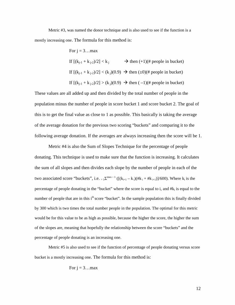
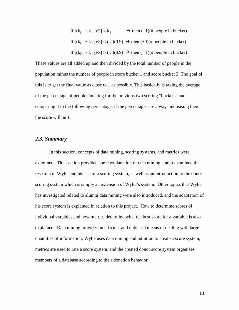
Metric #3, was named the donor technique and is also used to see if the function is a
mostly increasing one. The formula for this method is:
For j = 3…max
If [(k j-1 + k j-2)/2] < k j � then (+1)(# people in bucket)
If [(k j-1 + k j-2)/2] < (k j)(0.9) � then (±0)(# people in bucket)
If [(k j-1 + k j-2)/2] > (k j)(0.9) � then ( –1)(# people in bucket)
These values are all added up and then divided by the total number of people in the
population minus the number of people in score bucket 1 and score bucket 2. The goal of
this is to get the final value as close to 1 as possible. This basically is taking the average
of the average donation for the previous two scoring “buckets” and comparing it to the
following average donation. If the averages are always increasing then the score will be 1.
Metric #4 is also the Sum of Slopes Technique for the percentage of people
donating. This technique is used to make sure that the function is increasing. It calculates
the sum of all slopes and then divides each slope by the number of people in each of the
two associated score “buckets”, i.e. = 1Σmax – 1 ([(ki+1 – k i)(#k i + #k i+1)]/600). Where ki is the
percentage of people donating in the “bucket” where the score is equal to i, and #ki is equal to the
number of people that are in this ith score “bucket”. In the sample population this is finally divided
by 300 which is two times the total number people in the population. The optimal for this metric
would be for this value to be as high as possible, because the higher the score, the higher the sum
of the slopes are, meaning that hopefully the relationship between the score “buckets” and the
percentage of people donating is an increasing one.
Metric #5 is also used to see if the function of percentage of people donating versus score
bucket is a mostly increasing one. The formula for this method is:
For j = 3…max
13
If [(k j-1 + k j-2)/2] < k j � then (+1)(# people in bucket)
If [(k j-1 + k j-2)/2] < (k j)(0.9) � then (±0)(# people in bucket)
If [(k j-1 + k j-2)/2] > (k j)(0.9) � then ( –1)(# people in bucket)
These values are all added up and then divided by the total number of people in the
population minus the number of people in score bucket 1 and score bucket 2. The goal of
this is to get the final value as close to 1 as possible. This basically is taking the average
of the percentage of people donating for the previous two scoring “buckets” and
comparing it to the following percentage. If the percentages are always increasing then
the score will be 1.
2.3. Summary
In this section, concepts of data mining, scoring systems, and metrics were
examined. This section provided some explanation of data mining, and it examined the
research of Wylie and his use of a scoring system, as well as an introduction to the donor
scoring system which is simply an extension of Wylie’s system. Other topics that Wylie
has investigated related to alumni data mining were also introduced, and the adaptation of
his score system is explained in relation to this project. How to determine scores of
individual variables and how metrics determine what the best score for a variable is also
explained. Data mining provides an efficient and unbiased means of dealing with large
quantities of information, Wylie uses data mining and intuition to create a score system,
metrics are used to rate a score system, and the created donor score system organizes
members of a database according to their donation behavior.
14
This project encounters many of the same problems that researchers have to deal
with daily when analyzing massive amounts of data. WPI is one of many universities
that seek to use its database as a tool to provide information about donation behavior of
their donors, and to find a more time and cost efficient means of determining what
potential donors of their database are most likely to donate. This section focuses on a
score system and how a modified version of Wylie’s score system can be implemented
with the WPI donor database. With metrics used to rate the scores assigned in a score
system, the ranking of donors in the database can provide a reliable means of organizing
records of a database based on their likelihood to donate.
15
3. Exploring the Data
WPI opened in 1865 with its first graduating class in 1871. There have been
alumni for the past 135 years however the database provided by our sponsor contains
donation activity starting in 1983. There are some individuals in the database who
donated before 1983 but the 1983 donation records are the cumulative amount given
through 1983, and although there is information for 2007, this year is not complete
therefore donation activity it not accurate for the entire fiscal year. This section provides
a description of the variables in the data, how they were grouped, and the conclusions
that were drawn from the different types of variables. Some conclusions about key parts
of the database will also be mentioned, as well as references to the majority of the tables
in the Appendices of this report.
The WPI data contains 48,604 individuals and a total of $99,387,742.12 in
donations. The first column in the data contained this identification number for each
individual. The rest of the database includes 101 additional columns containing an
assortment of personal information as well as donation behavior for years 1983 to 2007.
Of the 48,604 individuals, 24,204 (49.80%) had made a donation and the average
donation for the database was $2,044.85. The average donation for the individuals who
did donate was $4,106.25.
While WPI has information about donors on file, especially if the donor attended
WPI at any point, the majority of the information found in the real database is self-
reported. Self-reported data can be unreliable however for this project it was assumed
that any bias in self reported data did not have an effect on conclusions drawn in
determining scores (Burstein 1985).
16
Table 3 provides the data extract key that was given by the alumni office and later
modified by Yi Jin (Jin 2006) explaining all 102 personal identification numbers in the
database. While there are only 67 variables listed below, row 66 actually contains
donation activity per fiscal year from 1983 to 2007 and row 67 contains donations in gift
club per fiscal year 1996 to 2007. Each fiscal year for these two variables is allotted its
own column in the database, with donation activity recorded in 25 columns and gift club
recorded in 12 columns, completing the 102 columns in the database.
Table 3: Modified Data Extract Key
1 PERSON_NUM Person number for data extract 2 CATEGORY Constituents best (primary) donor category 3 GENDER M/F/NA 4 BIRTH_YEAR 4-digit year of birth 5 MARRIED Married/Single/etc. 6 LEGACY Yes: the person's admission record indicated a legacy
relationship (no details available)
7 GPA [1] Number for those available, spaces for those unavailable, "N/A" for those not applicable
8 BS_YEAR WPI B.S. year 9 BS_MAJOR WPI B.S. major 10 MS_YEAR WPI M.S. year 11 MS_MAJOR WPI M.S. major 12 PHD_YEAR WPI Ph.D. year 13 PHD_MAJOR WPI Ph.D. major 14 CERT_YEAR WPI certificate year 15 CERT_MAJOR WPI certificate major 16 HONOR_YEAR WPI honorary degree year 17 HONOR_DEG WPI honorary degree 18 NON_WPI_DEG value if known (formatted as institution : degree code :
year : major) 19 WPI_SPS Yes: the spouse is a constituent 20 NUM_OF_CHILD Count of children 21 PREF_CLAS Preferred class year 22 HAD_SCHOLARSHIP Yes: had scholarship while at WPI 23 PRES_FND Yes: a Presidential Founder 24 LIFETIME_PAC Yes: a lifetime PAC[2] member
17
25 TRUSTEE Yes: a trustee of WPI 26 ADM_VOL Yes: involved in alumni/admissions 27 CLS_AGENT Yes: involved in solicitation structure 28 REUNION Yes: constituent attended reunion(s) 29 ALUM_VOLUNTEER Count of distinct number of activities (involved in/as
department advisory board, gold council, …, 42 possibilities)
30 ALUM_CLUB Count of distinct number of activities (Tech Old Timers, Polyclub, …)
31 ALUM_LEADER Count of distinct number of activities (involved in/as class officer, trustee search committee, fund board, …, 30 possibilities)
32 FRAT Name of fraternity/sorority, blank otherwise 33 SPORT_COUNT Count of varsity sports 34 VARSITY_SPRTS Concatenated list of varsity sports 35 WPI_AWD Yes: constituent received this award at WPI 36 TAYLOR_AWD Yes: constituent received this award at WPI 37 SCHWIEGER_AWD Yes: constituent received this award at WPI 38 GODDARD_AWD Yes: constituent received this award at WPI 39 GROGAN_AWD Yes: constituent received this award at WPI 40 BOYNTON_AWD Yes: constituent received this award at WPI 41 WASHBURN_AWD Yes: constituent received this award at WPI 42 RES_CITY Home city (permanent address) 43 RES_STATE Home state code 44 RES_ZIP Home zip code (5 or 9-digit format) 45 RES_COUNTRY Home country 46 TITLE Job title if known, blank if unknown 47 WORK_CITY Work city (business address) 48 WORK_STATE Work state code 49 WORK_ZIP Work zip code (5 or 9-digit format) 50 WORK_COUNTRY Work country 51 STU_CLUB Count of clubs (Outing Club, Science Fiction, Sport
Parachute, …) 52 STU_ARTS Count of arts and literature organizations (Masque,
Pathways, Peddler, …) 53 STU_INTL_CLUB Count of international clubs (Indian Students
Association, …) 54 STU_CLUB_SPORT Count of club sports (scuba, bowling, autocross, …) 55 STU_PROF_SOC Count of undergrad professional societies 56 STU_MUSIC Count of music band: glee club, baker's dozen, … 57 STU_CLS_OFF Count of class officer (freshman, sophomore, …) 58 STU_SCH_INVOLVE Count of school involvement (student activities board,
18
resident advisor) 59 STU_SPEC_PROG Count of special programs (undergraduate employment
tennis, …) 61 STU_HONOR_SOC Count of honor societies (Pershing Rifles, Sigma Mu
Epsilon, Skull, …) 62 STU_PROJECT_CTR Project Center Info (from the student courses) 63 ALU_PROJECT_CTR Project Center Info (from alumni activities) 64 GRAD_DISTINCTION H: graduated with high distinction, D: graduated with
distinction, and blank 65 ALUM_CONTACTS Contacts made as an alumnus (phone calls, personal
visits, …) 66 FISCAL_YEAR_X
(X: 1983~2007) Total gift and memo for the specific fiscal year [3]
67 GIFT_CLUB_X (X: 1996~2007)
Gift Club designation for the specific fiscal year
[1]. WPI Undergraduates do not have a “true” GPA. Standard “numerical equivalent for
passed courses” approved by the faculty was used. [2]. PAC stands for President’s Advisory Council. [3]. Note the 1983 number is a cumulative amount given up through 1983 when the
values were loaded into “Banner”. Also note that 2007 data only contains data from the first few months of the fiscal year.
3.1 Focus Population
Danny Yi’s research found only 24 of the 101 variables statistically significant
when he performed multiple regression analysis. A variable called CATEGORY assigns
a record in the database a title that best categorizes their relationship to WPI. There are
18 different categories in the data, including ALUM which refers to a recipient of a
Bachelor’s Degree, PRNT which refers to a parent of an Alum, FRND which refers to a
friend of the institution, or GRAD which refers to a recipient of a Graduate Degree. The
CATEGORY variable was divided into the 18 different categories and the donations
made in each category. It was found that individuals under the ALUM category had the
most complete information in their remaining 100 variables, with 24,027 ALUM in the
19
database, 49.43% of the entire population in the database donating $80,862,060.67. Also,
with the ALUM information in the database having the most complete amount of data in
its associated cells, a more accurate score system can be determined because there is a
larger quantity of variables that can be used in calculating metrics and calculating scores
for individual variables.
3.2 Removing Outliers in Alumni Database
The ALUM database contained 24,027 individuals, with 14,364 (59.78%)
donating a total of $80,862,060. The average donation per individual was $3,365, with a
median of $45 and a standard deviation of $61,183.
Any individual who donated an exceptionally large amount was removed before
testing the score systems because they would have an overwhelming impact metrics.
Any set of score factors that happened to capture some of the largest donations would be
rated highly by the metrics. Individuals with total donations more than 3 standard
deviations above the mean were removed for testing. With this choice, any individual
who donated more than $186,916.52 was removed. This group included 62 individuals
(0.26% of the database) with total donations $44,899,094; over 45% of the total
donations were made by these 62 individuals. For these 62 individuals, the average
donation was $724,178 and a standard deviation of $957,396. The remaining 23,965
individuals had an average donation of $1,500 with standard deviation of $8,496. Any
score system which captured the outliers would have appeared to be a good score system.
Working on the data set with outliers removed gives a better picture of the accuracy of
the score system on the general population of alumni.
20
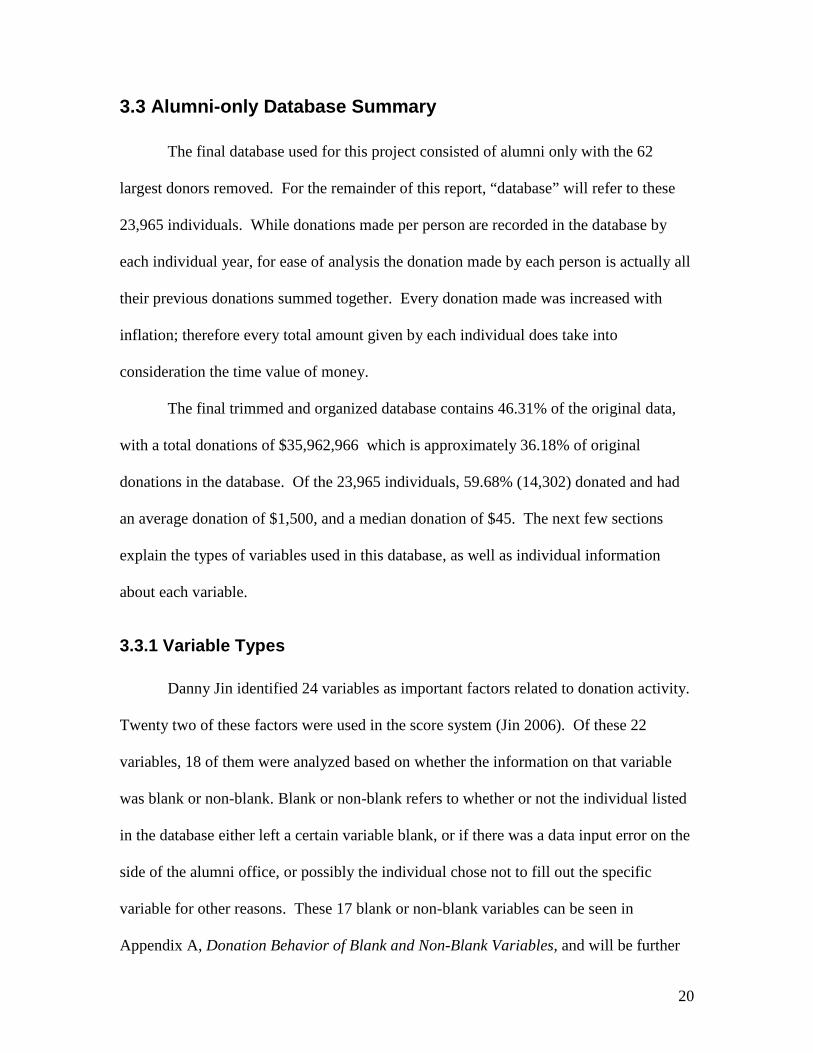
3.3 Alumni-only Database Summary
The final database used for this project consisted of alumni only with the 62
largest donors removed. For the remainder of this report, “database” will refer to these
23,965 individuals. While donations made per person are recorded in the database by
each individual year, for ease of analysis the donation made by each person is actually all
their previous donations summed together. Every donation made was increased with
inflation; therefore every total amount given by each individual does take into
consideration the time value of money.
The final trimmed and organized database contains 46.31% of the original data,
with a total donations of $35,962,966 which is approximately 36.18% of original
donations in the database. Of the 23,965 individuals, 59.68% (14,302) donated and had
an average donation of $1,500, and a median donation of $45. The next few sections
explain the types of variables used in this database, as well as individual information
about each variable.
3.3.1 Variable Types
Danny Jin identified 24 variables as important factors related to donation activity.
Twenty two of these factors were used in the score system (Jin 2006). Of these 22
variables, 18 of them were analyzed based on whether the information on that variable
was blank or non-blank. Blank or non-blank refers to whether or not the individual listed
in the database either left a certain variable blank, or if there was a data input error on the
side of the alumni office, or possibly the individual chose not to fill out the specific
variable for other reasons. These 17 blank or non-blank variables can be seen in
Appendix A, Donation Behavior of Blank and Non-Blank Variables, and will be further
21
explained in the following section. This blank and non-blank classification was
determined based on the information, or lack of information, available about the specific
variable, or the variable in question may have previously been established as a “yes or
blank” variable in the database.
RES_ZIP was analyzed differently than the other 21 variables because it used zip
codes to determine regions in Massachusetts and other locations outside of Massachusetts.
Of the 23,965 individuals in the ALUM database, 9,294 (38.78%) are listed as residents
of Massachusetts. A listing of all zip codes in Massachusetts, with their coinciding
county, and all zip codes outside of Massachusetts were used. Zip code organization for
Massachusetts residents only was done to divide the 9,294 individuals in Massachusetts
into their appropriate county.
The remaining 5 variables are classified as “multiple category” variables are
investigated individually in the next section. They are referred to as multiple category
variables because they have multiple significant answers and further conclusions could be
drawn from the variables multiple categories. The difference between multiple category
variables and blank and non-blank variables is that while blank and non-blank variables
assign a score to a variable simply based on whether any information was provided,
multiple category variables actually assign scores to the specific information that was
provided by that variable.
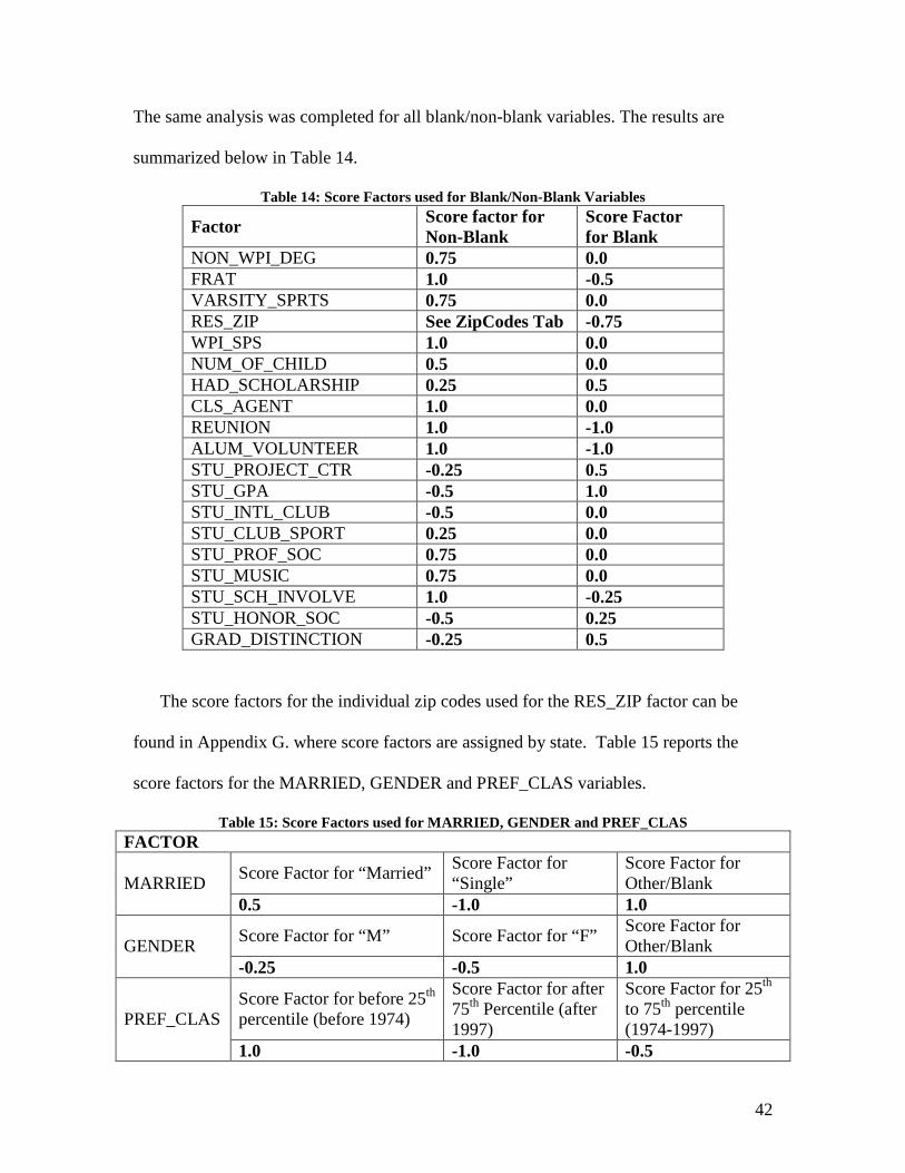
Appendix A, Donation Behavior of Blank and Non-Blank Variables, provides the
18 blank and non-blank variables, and below is an example of some conclusions that can
be drawn from the blank and non-blank variable FRAT. It can be seen below in Table 4
that 9,416 individuals said that they were in a fraternity. This means that 39.29% of the
22
records said they were in a fraternity or sorority, while the remaining 60.71% left this
variable blank or chose to not list themselves as being involved in a fraternity or sorority.
Then number of people listed as involved in a fraternity is reduced to the number of
people who were listed in a fraternity and who donated, this number was found to be
6,959. This means that of the individuals who identified themselves as being in a
fraternity, 73.91% donated. The total amount of donations made in this category was
$26,566,269.58 and dividing this by the 9,416 individuals listed as being in a fraternity
the average donation given by the FRAT variable is $2,821.40, with a median donation of
The final set of score factors reported above provided a good predictive model for
donations in the (trimmed) alumni database. Five different metrics were used to develop
a model that the metrics show that the score factors give good information about donation
behavior.
49
6. Conclusions
The goal of this project was to develop a scoring system that would use the
insight gained from Danny Jin’s statistical analysis (Jin 2006). The score system is a
tool that the Office of Development and Alumni Relations can use to organize and
explore its donor database. The system does not “predict” donations but it does identify
groups of donors that are more (or less) likely to make donations. It is designed to be as
simple and flexible as possible so that the Office of Development and Alumni Relations
can use the tool on current data and adapt it to future trends in donations.
The score system was tested on the 23,965 alumni in the donor database. Of the
102 variables for each individual, the score system uses 24 variables, assigning a score
factor (in the range -1.0 to +1.0) to values for each variable. For 18 of these variables, all
that was used was the fact that the value was not blank. For example, it did not matter
which fraternity or sorority the individual reported, it only mattered that the individual
had been involved in Greek life while at WPI. The score factors for each variable were
determined by comparing the effect that each value of the variable had on donations with
the donation statistics for the full population.
Three different metrics were developed to test the predictive ability of the score
system. A good score system would give larger scores to groups with better donation
behavior (frequency and amount). The final score system coded in Donor Score
System.xls satisfies this criterion.
50
References: Adriaans, Pieter; and Zantinge, Dolf (1996). Data Mining. Addison-Wesley Longman
Limited, Harlow, England. Pg. 47. Burstein, Leigh; Freeman, Howard; and Rossi, Peter (1985). Collecting Evaluation Data:
Problems and Solutions. Sage Publications, California. (page 51). Bryman, Alan; and Hardy, Melissa (2004). Handbook of Data Analysis. Sage Publications, California. Calkins, Keith G. The How and Why of Statistical Sampling. Andrews University, 1998-2005.
<http://www.andrews.edu/~calkins/math/webtexts/stat02.htm> 11/10/2006 Crawford, Jogoda and Frank. Data Mining in a Scientific Environment.
Data Description, Inc (2006). Margolis Wylie Associates Mines a Wealth of Information for Higher Education. http://www.datadesk.com/company/profiles/wylie.shtml 11/30/2006 Data Mining Examples & Testimonials, Data Mining Software of data mining solutions.
<http://www.data-mining-software.com/data_mining_examples.htm> 9/3/2006 Davies, Phil. The Magenta Book: Guidance Notes for Policy Evaluation and Analysis.
Government Chief Social Researcher’s Office, 2004. <http://www.policyhub.gov.uk/downloads/chapter5.pdf> 11/10/2006
Dictionary.com. “Coefficient of Correlation.” American Heritage Dictionary of the English Language, Fourth Edition (2006). Houghton Mifflin Company. <http://dictionary.reference.com/search?q=coefficient%20of%20correlation> 4/20/2007 Dmoz (2006). “Data Mining” <http://dmoz.org/Computers/Software/Databases/Data_Mining/> 9/2/2006 Draper, N.R., and Smith, H (1981). Applied Regression Analysis, second edition. John Wiley & Sons, Canada. Ebecken, Nelson (1998). Data Mining. WIT Press: Southhampton, UK. Fayyad, Usama. Piatetsky-Shpiro, Gregory. Smyth, Padhraic. From Data Mining to Knowledge Discovery in Databases. <http://www.aaai.org/AITopics/assets/PDF/AIMag17-03-2-article.pdf> 9/3/2006
51
Frank, Eibe; Witten, Ian (2000). Data Mining: Practical Machine Learning Tools and Techniques with Java Implementations. Morgan Kaufmann Publishers, San Francisco, California (2000). (Page 3)
Friedman, Jerome; Hastie, Trevor; and Tibshirani, Robert (2001). The Elements of Statistical Learning: Data Mining, Inference, and Prediction. Springer Series in Statistics. Springer-Verlag New York. InflationData.com (2003-2007). “Historical CPI-U data from 1913 to the present.” Financial Trend Forecaster, Capital Professional Services. <http://inflationdata.com/inflation/Consumer_Price_Index/HistoricalCPI.aspx?rsCPI_currentPage=2> 3/1/2007 Jin, Yi. “Regression Analysis of University Giving Data.” MS Project Report. Department of Mathematical Sciences. Worcester Polytechnic Institute, December 2006. Kutner, Michael H., Neter, John., and Wasserman, William (1990). Applied Linear Statistical Models: Regression, Analysis of Variance, and Experimental Designs, third edition. Richard D. Irwin. Kutner, Michael H., Nachtsheim, Christopher J., Neter, John, and Li, William (2005). Applied Linear Statistical Models, fifth edition. McGraw-Hill. Linux Information Project (2005). “Metric Definition.”
<http://www.bellevuelinux.org/metric.html> 3/23/2007 Microsoft Corporation (2006). “Data Mining” MSDN.
<http://forums.microsoft.com/msdn/showforum.aspx?forumid=81&siteid=1> 9/3/2006 Pyle, Dorian (1999). Data Preparation for Data Mining. Morgan Kaufmann Publishers, Inc. San Francisco, California. Saarenvirta, Gary (1998). Mining Customer Data. International Business Machines Corporation.
Wylie, Peter B (2004). Data Mining for Fund Raisers: How to use simple statistics to find the gold in your donor database (even if you hate statistics). Council for Advancement and Support of Education: Washington, DC. P. 11-72. Wylie, Peter B (2005). Deep Pockets: Where the Alumni Money Is. Council for
Advancement and Support of Education. <http://www.case.org/files/Bookstore/PDF/Wylie%20White%20Papers/Deep_Pockets_Where_the_Alumni_Money_Is.pdf> 9/14/2006
53
Appendix A: Donation Behavior of Blank and Non-Blan k Variables
Zip Min Zip Max State Score Factor 0 1000 NOT IN USE -0.75
1001 2791 MA 0.5 2792 2800 NOT IN USE -0.75 2801 2940 RI -1.0 2941 3030 NOT IN USE -0.75 3031 3897 NH 0.5 3898 3900 NOT IN USE -0.75 3901 4992 ME 0.5 4993 5000 NOT IN USE -0.75 5001 5495 VT 0.5 5496 5500 NOT IN USE -0.75 5501 5544 MA 0.5 5545 5600 NOT IN USE -0.75 5601 5907 VT 0.5 5908 6000 NOT IN USE -0.75 6001 6389 CT 0.75 6390 6390 NY 0.5 6391 6400 NOT IN USE -0.75 6401 6928 CT 0.75 6929 7000 NOT IN USE -0.75 7001 8989 NJ 1.0 8990 10000 NOT IN USE -0.75
10001 14975 NY 0.5 14976 15000 NOT IN USE -0.75 15001 19640 PA 1.0 19641 19700 NOT IN USE -0.75 19701 19980 DE 1.0 19981 20000 NOT IN USE -0.75 20001 20039 DC -1.0 20040 20167 VA 0.5 20168 20599 DC -1.0 20600 20797 MD 0.5 20798 20798 NOT IN USE -0.75 20799 20799 DC -1.0 20800 20811 NOT IN USE -0.75 20812 21930 MD 0.5 21931 22000 NOT IN USE -0.75
62
22001 24658 VA 0.5 24659 24700 NOT IN USE -0.75 24701 26886 WV 0.5 26887 27005 NOT IN USE -0.75 27006 28909 NC 0.5 28910 29000 NOT IN USE -0.75 29001 29948 SC 0.5 29949 30000 NOT IN USE -0.75 30001 31999 GA 0.5 32000 32003 NOT IN USE -0.75 32004 34997 FL 1.0 34998 35003 NOT IN USE -0.75 35004 36925 AL 0.5 36926 37009 NOT IN USE -0.75 37010 38589 TN 0.5 38590 38600 NOT IN USE -0.75 38601 39776 MS 0.5 39777 39900 NOT IN USE -0.75 39901 39901 GA 0.5 39902 40002 NOT IN USE -0.75 40003 42788 KY 0.5 42789 43000 NOT IN USE -0.75 43001 45999 OH 1.0 46000 46000 NOT IN USE -0.75 46001 47997 IN 0.5 47998 48000 NOT IN USE -0.75 48001 49971 MI 0.75 49972 50000 NOT IN USE -0.75 50001 52809 IA 0.5 52810 53000 NOT IN USE -0.75 53001 54990 WI 0.5 54991 55000 NOT IN USE -0.75 55001 56763 MN 0.5 56764 57000 NOT IN USE -0.75 57001 57799 SD 0.5 57800 58000 NOT IN USE -0.75 58001 58856 ND 0.5 58857 59000 NOT IN USE -0.75 59001 59937 MT -1.0 59938 60000 NOT IN USE -0.75 60001 62999 IL 1.0
63
63000 63000 NOT IN USE -0.75 63001 65899 MO 0.5 65900 66001 NOT IN USE -0.75 66002 67954 KS 0.5 67955 68000 NOT IN USE -0.75 68001 68118 NE 0.5 68119 68120 IA 0.5 68121 68121 NOT IN USE -0.75 68122 69367 NE 0.5 69368 70000 NOT IN USE -0.75 70001 71232 LA 0.5 71233 71233 MS 0.5 71234 71497 LA 0.5 71498 71600 NOT IN USE -0.75 71601 72959 AR 0.5 72960 73000 NOT IN USE -0.75 73001 73199 OK 0.5 73200 73300 NOT IN USE -0.75 73301 73301 TX 0.5 73302 73400 NOT IN USE -0.75 73401 74966 OK 0.5 74967 75000 NOT IN USE -0.75 75001 75501 TX 0.5 75502 75502 AR 0.5 75503 79999 TX 0.5 80000 80000 NOT IN USE -0.75 80001 81658 CO 0.5 81659 82000 NOT IN USE -0.75 82001 83128 WY 0.5 83129 83200 NOT IN USE -0.75 83201 83876 ID 0.5 83877 84000 NOT IN USE -0.75 84001 84784 UT 0.5 84785 85000 NOT IN USE -0.75 85001 86556 AZ 0.5 86557 87000 NOT IN USE -0.75 87001 88441 NM 0.5 88442 88509 NOT IN USE -0.75 88510 88589 TX 0.5 88590 88900 NOT IN USE -0.75 88901 89883 NV 0.5
64
89884 90000 NOT IN USE -0.75 90001 96162 CA 1.0 96163 96700 NOT IN USE -0.75 96701 96898 HI 0.5 96899 97000 NOT IN USE -0.75 97001 97920 OR 0.5 97921 98000 NOT IN USE -0.75 98001 99403 WA 0.5 99404 99500 NOT IN USE -0.75 99501 99950 AK 0.5 99951 99999 NOT IN USE -0.75
65
Appendix H: User’s Manual provided for Donor Score System
User’s manual for Donor Score System.xls
This is a user’s manual for Donor Score System.xls, an excel spreadsheet which will determine a score to predict the likelihood of a donation for individuals in the Alumni database. This manual includes a detailed description of how the data must be entered, and then will run through an example run of 100 Alumni.
74
Getting the Data When using this spreadsheet, it is critical that the data be entered correctly on the
spreadsheet. Further, the spreadsheet was developed only for WPI Alumni. This
means that the CATEGORY field should be “ALUM” for all those to be entered
into the spreadsheet. Using the spreadsheet for other categories will not produce
valid results. It is assumed that data will be taken from the Alumni Office database
and put into a spreadsheet. The following are the specific items needed. They
should be put in an Excel spreadsheet in the order shown:
TOTAL DONATION (Column X) The data should look similar to this:
Once you have checked over the data you are ready to open the Donor Score
System spreadsheet.
NOTE: The PERSON_NUMBER has been replaced with “######” for
confidentiality.
68
Opening the Spreadsheet
Find the file Donor Score System.xls and open it. You may immediately receive a
message explaining that the macros have been disabled due to the security level.
This message will look like this:
If this happens, you will need to click “OK ” and then on the menu bar go to the
Tools menu option and select Macro and then Security. In the resulting Security
dialog, change the security level to medium, then close the spreadsheet and try
opening it again.
This time when the excel spreadsheet is opened a security warning will pop-
up that looks like this:
69
Click on “Enable Macros” to open the spreadsheet.
The spreadsheet should open on the “Data” tab. If it does not, click on the
first tab in the spreadsheet that is labeled “Data”, as seen below. If the spreadsheet
has any data in it already or is not blank, be sure to click on the “Clear Data”
button, to clear out any remaining values.
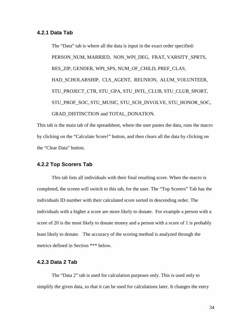
Data Tab
Clear Data Button
70
Running the Spreadsheet
At this point return to the Excel File with the Alumni data, where you should copy
all 24 factors for each individual. To do this, highlight all the alumni and their
factors. Copy all these values by holding down the “Ctrl” key and then typing “c”.
Return to the Donor Score System.xls and click on cell B1, and paste the data into
the spreadsheet by holding down the “Ctrl” key and typing “v”. Double check your
data to make sure that the data copied over right, and that all the Alumni factors are
lining up with the factors listed on the top row of the “Data” tab. You should now
have all the data in the spreadsheet, and it should look like this:
You are now ready to run the spreadsheet; click on the “Calculate Scores!” button.
71
When the calculations are done, the spreadsheet will automatically move to the
“Top Scorers” tab, with a list of all ID numbers and their respective scores in
descending order of the score, as seen below:
NOTE: This process can take hours for large amounts of data. A progress bar pops up to let you know the spreadsheet is working.
72
NOTE: The list of Top Scorers can be copied and moved to another spreadsheet or perhaps written back to the Alumni database for further reference.
Viewing the Results
Now that the calculations are complete you can review your results. There are a
total of 12 different tabs in this spreadsheet. Below is an enlarged image of all the
tabs.
• “Top Scorers” Tab
The “Top Scorers” Tab has, as mentioned, each individuals ID number and
their calculated score sorted in descending order by score. This is the most
important tab, as it ranks each individual as to how likely they are to donate.
The higher a score the more likely a person is to donate, and the higher the
donation amount will be. For example a person with a score of 20 is the
most likely to donate money and a person with a score of 1 is probably least
likely to donate. Because these scores were calculated using the factors in
the database, this does not always mean that it is completely accurate. It is
possible for a person with a score of 1 to give a significant donation, just as
it is possible for a person with a score of 20 to not donate at all. Ways to
measure if theses scores are accurate can be seen in graphs, and calculations
which are described later in this manual.
73
• “Data 2” Tab
The “Data 2” tab is used only for calculation purposes only. It simplifies the
given data, so that it can be used for calculations later, by turning many of
the values into “Y”, so that it can be easier converted to a numeric value
later.
• “ZipCodes” Tab
The “ZipCodes” tab is also used for calculation purposes. It has a list of all
zip codes currently used in the U.S. with a corresponding score that is used
for the calculation of the final score.
• “Score Factors” Tab
This tab is essential in calculating each individual’s score.
74
Above are the individual scorings that are associated with each piece of
information about each person. For example, in the diagram you can see that
for a person that does have a non WPI degree will receive .75 for that
individual piece of information, whereas someone who does not have a non
WPI degree (i.e. left it blank) will receive a 0.
There are factors for each piece of information about the individual. Some
are categorized as blank or non-blank, while others such as “Gender” have
different factors for “M”, “F”, and “Other” (e.g. “N”)
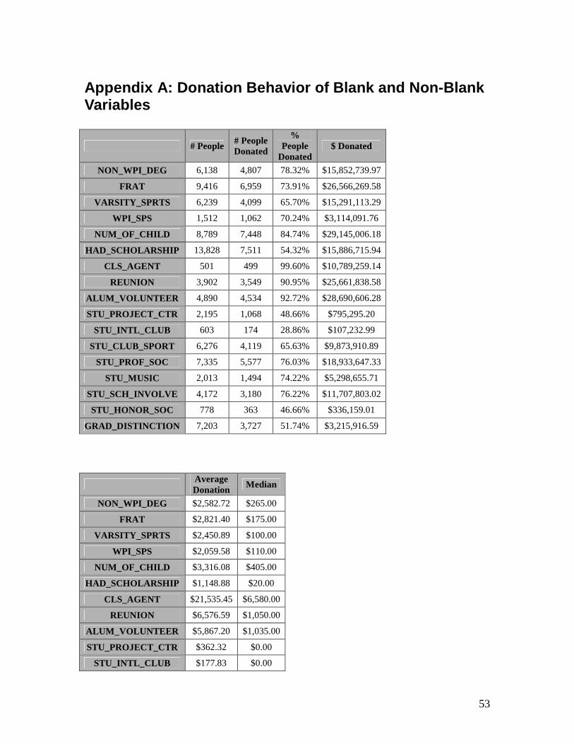
• “Scoring” Tab
The “Scoring” tab is where all the calculations occur. For each individual, it
looks at the “Data 2” and “Score Factors” tab, and the places the respective
factor for each piece of information. As seen in the screenshot below, each
individual ends up with 22 different factors based on their information,
which then get summed up for their Total Score. From the Total Score a
final calculation is done to adjust the scores so that they only range from 1 to
20. This is called the “ADJ Score”, which is used for all the graphs and is
shown on the “Top Scorers” Tab.
Factor for “NON_WPI_DEG” left blank
Factor used if “NON_WPI_DEG” is not blank
75
NOTE: To portray the most desirable results, for the remainder of this manual all screenshots are based on the 23,977 Alumni that the spreadsheet was run on.
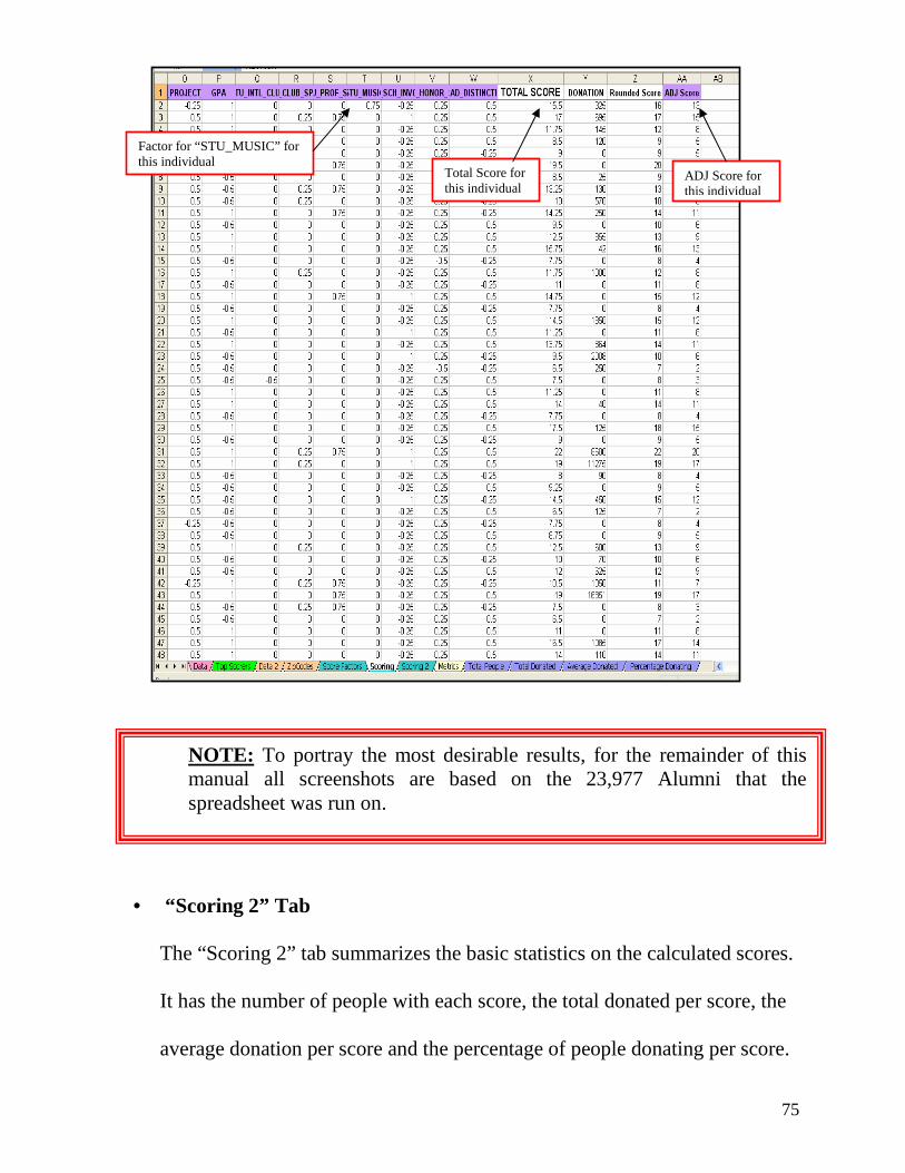
• “Scoring 2” Tab
The “Scoring 2” tab summarizes the basic statistics on the calculated scores.
It has the number of people with each score, the total donated per score, the
average donation per score and the percentage of people donating per score.
Factor for “STU_MUSIC” for this individual
Total Score for this individual
ADJ Score for this individual
76
The graphs are drawn using these statistics. This tab also shows the
minimum and maximum Total and Adjusted scores.
• “Metrics” Tab
The “Metrics” tab is used to see how good the scoring system currently is.
There are five different calculations;
1. 2R value on the average donation; 2. the Sum of slopes of average donation; 3. the comparison of averages for the average donation; 4. the Sum of slopes of the percentage of people donating and 5. the comparison of averages for the percentage of people donating.
While this manual does not include details on these calculations, you can
find them in the MQP paper. Each metric has a numeric value, and the sum
of all these values should be maximized with the sum of metrics 1, 3, and 5
as close to 3 as possible.
77
The shown example below is based on the 23,900+ database (in a database
of only 100, these score and sums would be very low). As you can see, this
fit is a good fit, because the sum of Metrics #1, #3 and #5 is almost 2.6.