Page 1
* Corresponding author: [email protected]
Huang, S., Zuo, W., Sohn, M. “Amelioration of the Cooling Load based Chiller Sequencing Control,”
Applied Energy, 168, pp. 204-215, 2016.
Amelioration of the Cooling Load based Chiller Sequencing Control
Sen Huang a, Wangda Zuo a,*, Michael D. Sohn b
a Department of Civil, Architectural and Environmental Engineering, University of Miami,
1251 Memorial Drive, Coral Gables, FL 33146, U.S.A. b Energy Analysis and Environmental Impacts Division, Lawrence Berkeley National Laboratory,
One Cyclotron Road, Berkeley, CA 94720, U.S.A.
Abstract:
Cooling Load based Control (CLC) for the chiller sequencing is a commonly used control strategy for
multiple-chiller plants. To improve the energy efficiency of these chiller plants, researchers proposed
various CLC optimization approaches, which can be divided into two groups: studies to optimize the load
distribution and studies to identify the optimal number of operating chillers. However, both groups have
their own deficiencies and do not consider the impact of each other. This paper aims to improve the CLC
by proposing three new approaches. The first optimizes the load distribution by adjusting the critical
points for the chiller staging, which is easier to be implemented than the existing approaches. In addition,
by considering the impact of the load distribution on the cooling tower energy consumption and the pump
energy consumption, this approach can achieve a better energy saving. The second optimizes the number
of the operating chillers by modulating the critical points and the condenser water set point in order to
achieve the minimal energy consumption of the entire chiller plant that may not be guaranteed by existing
approaches. The third combines the first two approaches to provide a holistic solution. The proposed three
approaches were evaluated via a case study. The results show that the total energy consumption saving for
the studied chiller plant is 0.5%, 5.3% and 5.6% by the three approaches, respectively. An energy saving
of 4.9% to 11.8% can be achieved for the chillers at the cost of more energy consumption by the cooling
towers (increases of 5.8% to 43.8%). The pumps’ energy saving varies from -8.6% to 2.0%, depending on
the approaches.
Keywords: Multiple-chiller Plant; Chiller Sequencing Control; Model-based Optimization
Page 2
2
1. Introduction
1.1 Background
In the United States, commercial building cooling equipment consumed around 77.4 GWh primary
energy in 2010 [1]. Chiller plants are widely used to provide cooling for large buildings, data centers and
district cooling systems. As major components of the chiller plants, chillers alone represented about 35%
of the energy consumption by the commercial building cooling [2]. Due to their significant energy
consumption, optimal control of the chiller plants is of great interest to the nation. To enhance the
operational efficiency of the chiller plants, many researchers have devoted efforts to achieve the optimal
control of the plants. As a result, many approaches have been proposed [3-43].
Among various configurations of chiller plants, the multiple-chiller plants are the most widely used. For
those plants, it is recommended to operate chillers sequentially rather than simultaneously [44]. To
operate chillers in sequence, one uses a chiller sequencing control, usually based on the cooling load, to
bring chillers online or offline. Depending on the approach to indicate the cooling load, the chiller
sequencing control can be categorized as: the return chilled water temperature based control, the bypass
flow based control, the direct power based control, and the Cooling Load based Control (CLC) [45].
Among them, the CLC is considered to be the most promising because other approaches employ the use
of indirect indicators of the cooling load (e.g. the return chilled water temperature, the volume flow rate at
bypass of secondary loop, and the chiller power), which may not be proportional to the cooling load [21].
The CLC directly calculates the cooling load using the chilled water flow rate and the difference between
the chilled water supply temperature and return temperature [9].
In the CLC, one chiller will not be brought online/offline unless the cooling load is larger/smaller than the
total available cooling capacity of the operating chillers. The total available cooling capacity of 𝑖
operating chillers can be referred as a Critical Point (CP):
𝐶𝑃𝑖 = ∑ 𝐶𝐶𝑎𝑐𝑡,𝑗𝑖𝑗=1 , (1)
where 𝐶𝐶𝑎𝑐𝑡,𝑗 is the actual cooling capacity of the 𝑗𝑡ℎ chiller. In the real world implementation, the
nominal capacity of the chiller, 𝐶𝐶𝑛𝑜𝑚,𝑗, is conventionally used to represent 𝐶𝐶𝑎𝑐𝑡,𝑗. Thus, equation (1)
can be converted into:
𝐶𝑃𝑖 = 𝜂 ∑ 𝐶𝐶𝑛𝑜𝑚,𝑗𝑖𝑗=1 , (2)
where 𝜂 is the safety factor (e.g., 90%) to mitigate the risk of insufficient cooling supply during the chiller
start-up period. Besides, a state machine [46] can also be used to facilitate the implementation of the CLC.
To avoid a chiller short circling, a waiting time 𝑡𝑤𝑎𝑖𝑡 and a dead band 𝐶𝑃𝑑𝑏 are usually employed. For
Page 3
3
instance, Figure 1 shows a conventional CLC for a chiller plant with three identical chillers. The
transition between states indicates adding or reducing the number of the operating chillers.
Figure 1 The state machine of a conventional CLC for a chiller plant with three identical chillers
1.2 CLC Optimization
Although widely used, the conventional CLC has limitations and can’t guarantee the minimal energy
consumption by the chiller plants. To improve the energy efficiency of the chiller plants, researchers
proposed various CLC optimization approaches [5-7, 9, 20-33, 40-43]. Generally speaking, those
approaches can be divided into two groups: studies to optimize the load distribution and studies to
identify the optimal number of operating chillers. We will discuss the concept and the limitations of each
group as follows.
The first group aims to optimize the load distribution among the chillers. The conventional CLC turns on
an additional chiller only when the cooling loading approaches the total nominal cooling capacity of the
operating chillers. This means that chillers will work at the highest Partial Load Ratio (PLR). The PLR is
the ratio of the cooling load handled by one chiller to its nominal cooling capacity. However, the
ASHRAE Handbook [44] points out that a higher chiller PLR does not necessarily mean a higher
operational efficiency. The chiller’s operational efficiency is usually measured by the coefficient of
performance (COP), which is the ratio of the cooling energy provided by the chiller to its power
consumption. Figure 2 shows that the highest COPs may occur at relatively low PLRs for three different
chillers.
AllOff
OneOn
TwoOn
On
Load > CP1 + CPdb
(Waiting Period = twait)
Load > CP2 + CPdb
(Waiting Period = twait)
Off
AllOn
Load < CP1 - CPdb
(Waiting Period = twait)
Load < CP2 - CPdb
(Waiting Period = twait)
Page 4
4
Figure 2 The relationship between PLRs and the relative COPs for three different chillers calculated
according to the chiller dataset provided by EnergyPlus [47]
To achieve the optimal load distribution, researchers developed model based optimization approaches to
adjust the PLR of each chiller individually according to a given cooling load [5, 7, 22-33]. Some studies
aimed to maximize a summation of the operating chillers’ COP as follows [5, 22, 24, 33]:
𝐽 = max(∑ 𝐶𝑂𝑃𝑖𝑀𝑖=1 ),
s.t. (3)
∑ 𝑃𝐿𝑅𝑖𝐶𝐶𝑛𝑜𝑚,𝑖𝑀𝑖=1 = �̇�, (4)
where 𝐶𝑂𝑃𝑖 and 𝑃𝐿𝑅𝑖 are the COP and PLR of the 𝑖th chiller, respectively. The 𝑀 is the number of the
chillers in the chiller plant and �̇� is the cooling load. They utilized a regressed PLR-COP curve in
equation (5) to calculate the 𝐶𝑂𝑃𝑖 under the 𝑃𝐿𝑅𝑖:
𝐶𝑂𝑃𝑖 = ∑ 𝑎𝑗𝑃𝐿𝑅𝑖𝑗𝑚
𝑗=0 , (5)
where 𝑎𝑗 is the 𝑗th constant coefficient and 𝑚 is the number of the constant coefficients.
Other approaches tried to minimize the sum of the chillers’ power as follows [7, 23, 25-32]:
𝐽 = min(∑ 𝑃𝑐ℎ,𝑖𝑀𝑖=1 ),
s.t. (6)
∑ 𝑃𝐿𝑅𝑖𝐶𝐶𝑛𝑜𝑚,𝑖𝑀𝑖=1 = �̇�, (7)
where 𝑃𝑐ℎ,𝑖 is the power of the 𝑖th chiller. The regressed Power-PLR curve in equation (8) was employed
to calculate 𝑃𝑐ℎ,𝑖.
𝑃𝑐ℎ,𝑖 = ∑ 𝑏𝑗𝑃𝐿𝑅𝑖𝑗𝑛
𝑗=0 , (8)
where 𝑏𝑗 is the 𝑗th constant coefficient and 𝑛 is the number of the constant coefficients.
Page 5
5
Both the above approaches used the PLRs as the independent variables to directly/indirectly reduce the
total power of the chillers. However, it is difficult to implement the PLR control in the real world
application since the PLR can only be indirectly controlled. Some scholars improved the above
approaches by replacing the PLRs with other relevant controllable parameters, such as the chilled water
flow rates through each chiller [6, 40], the temperature set points of the chilled water leaving each chiller
[41, 42], and the combination of the previous two parameters [43]. However, these approaches still have
some limitations. For instance, the approaches of adjusting the chilled water flow rate through chillers can
only be applied to the chiller plant equipped with chillers and pumps that can handle variable chilled
water flow rates. In addition, these approaches only consider the impact of the load distribution on the
chiller power. However, for plants with dedicated pumps and dedicated cooling tower for each chiller, the
load distribution also impacts the pump power and the cooling tower power. Without considering the
impacts on the pump power and the cooling tower power, these approaches can’t guarantee the minimal
energy consumption for the entire chiller plant.
The second group is associated with the optimization on the number of the operating chillers. As
mentioned above, the conventional CLC uses the chillers’ nominal cooling capacities to represent the
chillers’ actual cooling capacities. However, the actual cooling capacity of a chiller varies by its operating
conditions [9, 21]. As shown in Figure 3, a chiller’s capacity increases up to 110% of its nominal capacity
when the temperature of the condenser water entering the chiller (𝑇𝑐𝑤,𝑒𝑛𝑡 ) decreases from 23.89oC
(nominal condition) to 18.89oC. Therefore, it is possible that a chiller’s actual cooling capacity is larger
than its nominal capacity and so does the entire multi-chiller plant. In this case, the chiller plant can meet
a higher cooling load without turning on an additional chiller. Since we usually have a dedicated primary
chilled water pump and a dedicated condenser water pump for each chiller, reducing the number of the
operating chillers can save energy from the dedicated pumps [44].
Page 6
6
Figure 3 The relationship between the temperature of the condenser water entering the chiller and the
relative cooling capacity for three different chillers calculated according to the chiller dataset
provided by EnergyPlus [47]
To identify the optimal number of the operating chillers, some researchers proposed to reset the CPs
based on the estimation of the actual cooling capacity [9, 20, 21]. They calculated 𝐶𝐶𝑎𝑐𝑡,𝑖 using the
operating parameters of the chiller (such as the pressure in the evaporator, compressibility factor and so
on) at a given operating condition. Although these approaches may reduce the pump energy consumption,
they can’t guarantee the minimal energy consumption of the entire chiller plant including chillers, cooling
towers and pumps. For instance, by increasing the CPs according to the calculated cooling capacities, it is
possible to reduce the number of the operating chillers. In that case, the PLR of each operating chiller has
to increase to meet the same cooling load with fewer chillers. As we mentioned above, the increased
PLRs may lead to lower COPs.
To summarize, there are deficiencies in the existing CLC optimization approaches. In addition, although
the optimization of the load distribution and the optimization of the number of the operating chillers
interact with each other, they were only studied separately in previous studies. In response to these issues,
we propose three new CLC optimization approaches. The first approach is to optimize the load
distribution by adjusting the CPs. The second approach is to optimize the number of the operating chillers
by modulating the CPs and the condenser water set point. The third approach combines the first two
approaches aiming to achieve more energy savings with a holistic solution.
Page 7
7
This paper makes contributions to the literature in a number of ways: first, we developed a new approach
for the optimal load distribution. This approach is easier to be implemented than existing approaches in
literature and can achieve a better energy performance for the entire chiller plant. Second, we proposed a
new approach to optimize the number of the operating chillers. This approach considers the impact of the
CPs reset on the energy performance of the chillers, the cooling towers and the pumps, which is not
considered in the existing approaches. Third, we provided a holistic solution to address the optimal load
distribution problem and the optimal number of the operating chillers problem simultaneously, which has
not been reported in the literature yet to our knowledge.
The paper is organized as follows: after the introduction, we introduce the three new approaches for the
CLC optimization. We then elaborate the implementation of these approaches. Finally, we evaluate the
performances of these approaches via a case study.
2. New Approaches for the CLC optimization
2.1 General Assumptions
In this paper, we consider a water-cooled chiller plant with 𝑀 chillers and 𝑁 cooling towers. Each chiller
has a dedicated constant speed chilled water pump and a dedicated constant speed condenser water pump.
The towers have variable cooling tower fans controlled by the same set point for the temperature of the
condenser water leaving the towers, which is called condenser water set point, 𝑇𝑐𝑤,𝑠𝑒𝑡. The other control
parameters except the CPs and 𝑇𝑐𝑤,𝑠𝑒𝑡, such as set points for the temperature of the chilled water leaving
the chillers, 𝑇𝑐ℎ𝑤,𝑠𝑒𝑡, are constant. Thus, the total power of chillers, pumps, and cooling towers, 𝑃𝑡𝑜𝑡, at
time 𝑡 can be described as follows:
𝑃𝑡𝑜𝑡(𝑡) = ∑(𝑃𝑐ℎ,𝑖
𝑀
𝑖
(𝑡) + 𝑃𝑝𝑢,𝑖(𝑡)) + ∑ 𝑃𝑡𝑤,𝑗(𝑡)
𝑁
𝑗
= 𝑓1(𝑇𝑐𝑤,𝑠𝑒𝑡(𝑡), 𝐶𝑃1(𝑡), … , 𝐶𝑃𝑀−1(𝑡), �̇�(𝑡), 𝑇𝑤𝑏(𝑡), 𝑆(𝑡)),
(9)
where 𝑃𝑝𝑢,𝑖 and 𝑃𝑡𝑤,𝑗 is the power of the dedicated chilled water pump and the dedicated condenser water
pump for the 𝑖th chiller and the 𝑗th cooling tower, respectively. The 𝑇𝑤𝑏 is the wet bulb temperature and 𝑆
is the state vector of the system (e.g. equipment operating status, water temperature in the condenser and
the evaporator of the chiller). Then the energy consumption of the chiller plant for a period from 𝑡0 to
𝑡0 + ∆𝑡, 𝐸𝑡𝑜𝑡|𝑡0
𝑡0+Δ𝑡, is
Page 8
8
𝐸𝑡𝑜𝑡|𝑡0
𝑡0+Δ𝑡= ∫ 𝑃𝑡𝑜𝑡(𝑡)𝑑𝑡
𝑡0+∆𝑡
𝑡0=
∫ 𝑓1(𝑇𝑐𝑤,𝑠𝑒𝑡(𝑡), 𝐶𝑃1(𝑡), … , 𝐶𝑃𝑀−1(𝑡), �̇�(𝑡), 𝑇𝑤𝑏(𝑡), 𝑆(𝑡))𝑑𝑡𝑡0+∆𝑡
𝑡0.
(10)
The wet bulb temperature and the cooling load during the period of [t0, t0 +Δt] can be obtained from
the weather forecast and by using regression models, respectively. Then we can use the predicted cooling
load, �̇�𝑃, and the predicted wet bulb temperature, 𝑇𝑤𝑏𝑃, to represent �̇� and 𝑇𝑤𝑏 in the optimization:
�̇�(𝑡) = �̇�𝑃(𝑡), (11)
𝑇𝑤𝑏(𝑡) = 𝑇𝑤𝑏𝑃(𝑡). (12)
We assumed 𝐶𝑃𝑖(𝑡) and 𝑇𝑐𝑤,𝑠𝑒𝑡(𝑡) were constant during the period of [𝑡0, 𝑡0 + Δ𝑡]:
𝑇𝑐𝑤,𝑠𝑒𝑡(𝑡) = 𝑇𝑐𝑤,𝑠𝑒𝑡(𝑡0), (13)
𝐶𝑃𝑖(𝑡) = 𝐶𝑃𝑖(𝑡0). (14)
In addition, since 𝑆(𝑡) is a function of 𝑆(𝑡0), equation (10) can be converted into:
𝐸𝑡𝑜𝑡|𝑡0
𝑡0+Δ𝑡 = ∫ 𝑓2(𝑇𝑐𝑤,𝑠𝑒𝑡(𝑡0), 𝐶𝑃1(𝑡0), … , 𝐶𝑃𝑀−1(𝑡0), �̇�𝑃(𝑡), 𝑇𝑤𝑏
𝑃(𝑡), 𝑆(𝑡0))𝑑𝑡𝑡0+∆𝑡
𝑡0. (15)
2.2 The New Approaches
2.2.1 Approach 1: Optimal Load Distribution
For the load distribution optimization, we assumed 𝑇𝑐𝑤,𝑠𝑒𝑡 is constant, thus equation (15) can be changed
to:
𝐸𝑡𝑜𝑡|𝑡0
𝑡0+Δ𝑡 = ∫ 𝑓3( 𝐶𝑃1(𝑡0), … , 𝐶𝑃𝑀−1(𝑡0), �̇�𝑃(𝑡), 𝑇𝑤𝑏
𝑃(𝑡), 𝑆(𝑡0))𝑑𝑡𝑡0+∆𝑡
𝑡0. (16)
We used the CPs to replace PLRs as the independent variables to minimize 𝐸𝑡𝑜𝑡|𝑡0
𝑡0+Δ𝑡. Based on equation
(16), the optimization problem can be defined as
𝐽 = min(𝐸𝑡𝑜𝑡|𝑡0
𝑡0+Δ𝑡) =
min (∫ 𝑓3( 𝐶𝑃1(𝑡0), … , 𝐶𝑃𝑀−1(𝑡0), �̇�𝑃(𝑡), 𝑇𝑤𝑏𝑃(𝑡), 𝑆(𝑡0))𝑑𝑡
𝑡0+∆𝑡
𝑡0),
s.t.
(17)
𝐶𝑃1𝑚𝑖𝑛 < 𝐶𝑃1(𝑡0) ≤ 𝜂 ∑ 𝐶𝐶𝑛𝑜𝑚,𝑗
1𝑗=1 , (18)
𝐶𝑃𝑖−1(𝑡0) < 𝐶𝑃𝑖(𝑡0) ≤ 𝜂 ∑ 𝐶𝐶𝑛𝑜𝑚,𝑗𝑖𝑗=1 (𝑖 > 1), (19)
where 𝐶𝑃1𝑚𝑖𝑛 is the low bound for 𝐶𝑃1(𝑡0). The �̇�𝑃(𝑡), 𝑇𝑤𝑏
𝑃(𝑡) and 𝑆(𝑡0) are the input variables while
𝐶𝑃1(𝑡0), … , 𝐶𝑃𝑀−1(𝑡0) are the independent variables in the optimization. Approach 1 does not consider
Page 9
9
the change of chiller cooling capacities by the operating conditions, thus the high bounds for CPs are
determined as 𝜂 ∑ 𝐶𝐶𝑛𝑜𝑚,𝑗𝑖𝑗=1 .
Compared to the existing optimal load distribution approaches [5, 7, 22-33], Approach 1 has the
following advantages: first, it is easier for implementation since CPs can be directly adjusted; second, the
impact of the load distribution on the energy consumption by the cooling towers and the pumps is
considered in the objective function. Thus, Approach 1 can lead to a better energy saving for the entire
chiller plant.
2.2.2 Approach 2: Optimal Number of the Operating Chillers
For the cooling capacity based CPs reset, we changed the reset into an optimization problem based on
equation (15) to minimize 𝐸𝑡𝑜𝑡|𝑡0
𝑡0+Δ𝑡:
𝐽 = min(𝐸𝑡𝑜𝑡|𝑡0
𝑡0+Δ𝑡) =
min (∫ 𝑓2(𝑇𝑐𝑤,𝑠𝑒𝑡(𝑡0), 𝐶𝑃1(𝑡0), … , 𝐶𝑃𝑀−1(𝑡0), �̇�𝑃(𝑡), 𝑇𝑤𝑏𝑃(𝑡), 𝑆(𝑡0))𝑑𝑡
𝑡0+∆𝑡
𝑡0),
s.t.
(20)
𝑇𝑐𝑤,𝑠𝑒𝑡,𝐿 ≤ 𝑇𝑐𝑤,𝑠𝑒𝑡(𝑡0) ≤ 𝑇𝑐𝑤,𝑠𝑒𝑡,𝐻, (21)
𝜂 ∑ 𝐶𝐶𝑛𝑜𝑚,𝑗𝑖𝑗=1 ≤ 𝐶𝑃𝑖(𝑡0) ≤ 𝐶𝑃𝑖
𝑚𝑎𝑥, (22)
where 𝑇𝑐𝑤,𝑠𝑒𝑡,𝐿 and 𝑇𝑐𝑤,𝑠𝑒𝑡,𝐻 is the low bound and the high bound for 𝑇𝑐𝑤,𝑠𝑒𝑡(𝑡0), 𝐶𝑃𝑖𝑚𝑎𝑥 is the high
bound for 𝐶𝑃𝑖. The �̇�𝑃(𝑡) , 𝑇𝑤𝑏𝑃(𝑡) and 𝑆(𝑡0) are the input variables. The 𝑇𝑐𝑤,𝑠𝑒𝑡 is selected as an
independent variable because 𝑇𝑐𝑤,𝑠𝑒𝑡 can be used to regulate 𝑇𝑐𝑤,𝑒𝑛𝑡 which in turn affects the actual
cooling capacity of the chillers. The CPs can directly impact the number of the operating chillers and the
associated pumps. To reduce the number of the operating chillers and the operating pumps, we used
𝜂 ∑ 𝐶𝐶𝑛𝑜𝑚,𝑗𝑖𝑗=1 as the low bound for CPs and allowed CPs to be higher values up to 𝐶𝑃𝑖
𝑚𝑎𝑥.
Because the chiller cooling capacities vary by operating conditions, it is possible that we may not be able
to provide sufficient cooling if the estimated 𝐶𝑃𝑖𝑚𝑎𝑥 is larger than the actual maximum capacity. In that
case, we may save energy by reducing the number of the operating chillers and the associated pumps, but
the thermal comfort in the demand side would be sacrificed since provided cooling is insufficient. We
used the deviation of temperature of chilled water leaving the chiller, 𝑇𝑐ℎ𝑤,𝑙𝑒𝑎 , from 𝑇𝑐ℎ𝑤,𝑠𝑒𝑡 as an
indicator to determine if sufficient cooling is supplied. The deviation, 𝐷𝑐ℎ𝑤,𝑙𝑒𝑎, is calculated by
Page 10
10
𝐷𝑐ℎ𝑤,𝑙𝑒𝑎 = ∫ |𝑇𝑐ℎ𝑤,𝑙𝑒𝑎(𝑡) − 𝑇𝑐ℎ𝑤,𝑠𝑒𝑡|𝑑𝑡𝑡0+∆𝑡
𝑡0
(23)
Ideally, 𝐷𝑐ℎ𝑤,𝑠𝑒𝑡 should be equal to 0. However, the deviation may also be caused by the waiting time in
the CLC which is inevitable. With that in mind, we designed the following constraint:
𝐷𝑐ℎ𝑤,𝑙𝑒𝑎 ≤ 𝐷𝑐ℎ𝑤,𝑙𝑒𝑎,𝑏𝑎𝑠𝑒, (24)
where 𝐷𝑐ℎ𝑤,𝑠𝑒𝑡,𝑏𝑎𝑠𝑒 is 𝐷𝑐ℎ𝑤,𝑠𝑒𝑡 at the baseline in which no optimization occurs.
To summarize, the optimization can be described as:
𝐽 = min(𝐸𝑡𝑜𝑡|𝑡0
𝑡0+Δ𝑡) =
min (∫ 𝑓2(𝑇𝑐𝑤,𝑠𝑒𝑡(𝑡0), 𝐶𝑃1(𝑡0), . . , 𝐶𝑃𝑀−1(𝑡0), �̇�𝑃(𝑡), 𝑇𝑤𝑏𝑃(𝑡), 𝑆(𝑡0))𝑑𝑡
𝑡0+∆𝑡
𝑡0),
s.t.
(25)
𝑇𝑐𝑤,𝑠𝑒𝑡,𝐿 ≤ 𝑇𝑐𝑤,𝑠𝑒𝑡(𝑡0) ≤ 𝑇𝑐𝑤,𝑠𝑒𝑡,𝐻, (26)
𝜂 ∑ 𝐶𝐶𝑛𝑜𝑚,𝑗𝑖𝑗=1 ≤ 𝐶𝑃𝑖(𝑡0) ≤ 𝐶𝑃𝑖
𝑚𝑎𝑥, (27)
𝐷𝑐ℎ𝑤,𝑙𝑒𝑎 ≤ 𝐷𝑐ℎ𝑤,𝑙𝑒𝑎,𝑏𝑎𝑠𝑒 . (28)
Approach 2 considers the impact of the CPs reset on the energy performance of the chillers, the cooling
towers and the pumps. Thus it can guarantee the minimal energy consumption for the entire chiller plant,
which may not be achieved by the existing CPs reset approaches [9, 20, 21].
2.2.3 Approach 3: A Holistic Solution for the CLC
It is possible to save more energy by combining Approach 1 and Approach 2. In this holistic approach,
the CLC optimization problem can be defined as:
𝐽 = min(𝐸𝑡𝑜𝑡|𝑡0
𝑡0+Δ𝑡) =
min (∫ 𝑓2(𝑇𝑐𝑤,𝑠𝑒𝑡(𝑡0), 𝐶𝑃1(𝑡0), … , 𝐶𝑃𝑀−1(𝑡0), �̇�𝑃(𝑡), 𝑇𝑤𝑏𝑃(𝑡), 𝑆(𝑡0))𝑑𝑡
𝑡0+∆𝑡
𝑡0),
s.t.
(29)
𝑇𝑐𝑤,𝑠𝑒𝑡,𝐿 ≤ 𝑇𝑐𝑤,𝑠𝑒𝑡(𝑡0) ≤ 𝑇𝑐𝑤,𝑠𝑒𝑡,𝐻, (30)
𝐶𝑃1𝑚𝑖𝑛 < 𝐶𝑃1(𝑡0) ≤ 𝐶𝑃1
𝑚𝑎𝑥 , (31)
𝐶𝑃𝑖−1(𝑡0) < 𝐶𝑃𝑖(𝑡0) ≤ 𝐶𝑃𝑖𝑚𝑎𝑥 (𝑖 > 1), (32)
𝐷𝑐ℎ𝑤,𝑙𝑒𝑎 ≤ 𝐷𝑐ℎ𝑤,𝑙𝑒𝑎,𝑏𝑎𝑠𝑒. (33)
The �̇�𝑃(𝑡), 𝑇𝑤𝑏𝑃(𝑡) and 𝑆(𝑡0) are the input variables while 𝑇𝑐𝑤,𝑠𝑒𝑡(𝑡0), 𝐶𝑃1(𝑡0), … , 𝐶𝑃𝑀−1(𝑡0) are the
independent variables.
Page 11
11
2.3 Implementation
2.3.1 Constraints Setting
The CLC optimizations described in Approach 1, Approach 2 and Approach 3 are all constrained
optimization problems. The commonly used technologies for solving the constrained optimization
problems include the barrier function method and the penalty function method [48]. On one hand, the
barrier function method imposes a punishment on the value of the objective function if the value of the
objective function approaches the feasible region boundary. On the other hand, the penalty function
method adds a term to the objective function and the added term generates a negative impact on the
objective function when constrains are violated. In our CLC optimization, 𝑇𝑐𝑤,𝑠𝑒𝑡(𝑡0) and/or 𝐶𝑃𝑖(𝑡0),
which make 𝐷𝑐ℎ𝑤,𝑙𝑒𝑎 = 𝐷𝑐ℎ𝑤,𝑙𝑒𝑎,𝑏𝑎𝑠𝑒, can be optimal values, which is not allowed in the barrier function
method. Thus, we adopted the penalty function method. For example, the optimization problem in
Approach 3 can be converted into:
𝐽∗ = min (∫ 𝑓2(𝑇𝑐𝑤,𝑠𝑒𝑡(𝑡0), 𝐶𝑃1(𝑡0), … , 𝐶𝑃𝑀−1(𝑡0), �̇�𝑃(𝑡), 𝑇𝑤𝑏𝑃(𝑡), 𝑆(𝑡0))𝑑𝑡
𝑡0+∆𝑡
𝑡0+ 𝑘 ∙
max (0, 𝐷𝑐ℎ𝑤,𝑙𝑒𝑎 − 𝐷𝑐ℎ𝑤,𝑙𝑒𝑎,𝑏𝑎𝑠𝑒)),
s.t.
(34)
𝑇𝑐𝑤,𝑠𝑒𝑡,𝐿 ≤ 𝑇𝑐𝑤,𝑠𝑒𝑡(𝑡0) ≤ 𝑇𝑐𝑤,𝑠𝑒𝑡,𝐻, (35)
𝐶𝑃1𝑚𝑖𝑛 < 𝐶𝑃1(𝑡0) ≤ 𝐶𝑃1
𝑚𝑎𝑥, (36)
𝐶𝑃𝑖−1(𝑡0) < 𝐶𝑃𝑖(𝑡0) ≤ 𝐶𝑃𝑖𝑚𝑎𝑥 (𝑖 > 1), (37)
where 𝑘 is the iteration index of one optimization and max (0, 𝐷𝑐ℎ𝑤,𝑙𝑒𝑎 − 𝐷𝑐ℎ𝑤,𝑙𝑒𝑎,𝑏𝑎𝑠𝑒) is the term for the
penalty function method.
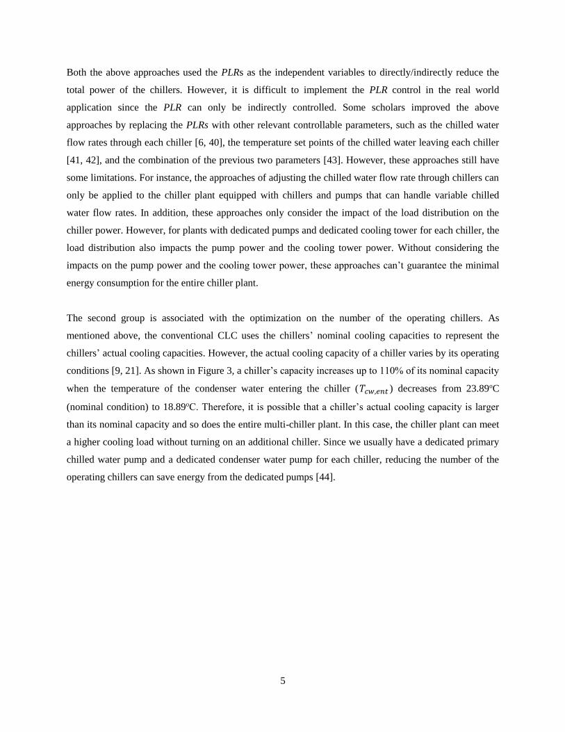
2.3.2 Optimization Framework
To enable the CLC optimization described in Section 2.2, we developed an optimization framework
(Figure 4). The �̇�𝑃(𝑡), 𝑇𝑤𝑏𝑃(𝑡) and 𝑆(𝑡0) are used as input variables. Then the generated optimal 𝐶𝑃𝑖(𝑡0)
and/or 𝑇𝑐𝑤,𝑠𝑒𝑡(𝑡0) will then be used to obtain 𝑆(𝑡0 + ∆𝑡) as initial values for the next optimization period
starting from 𝑡0 + ∆𝑡.
Page 12
12
Figure 4 The optimization framework
3. Case Study
3.1 Case Description
3.1.1 Configuration of the Chiller Plant
We studied a chiller plant with three identical chillers, three identical chilled water pumps, three identical
condenser water pumps, and three identical cooling towers (show in Figure 5). Each chiller has one
dedicated chilled water pump, one dedicated condenser water pump and one dedicated cooling tower. The
model of the chiller is a York_YK2771kW, which has the nominal cooling capacity as 2,771 kW (788
ton). For the cooling tower, the nominal fan power is 37 kW (50 HP) and was assumed to be proportional
to the cubic of the fan speed ratio. The nominal wet bulb temperature and the nominal approach
temperature is 23.89oC (75.00oF) and 0.89oC (1.60oF), respectively. The chilled water and the condenser
water pumps are constant speed pumps and their powers are 34 kW and 47 kW, respectively. In the
condenser water loop, a three-way valve is employed to modulate the condenser flow rates through the
cooling towers so that the temperature of the condenser water entering the chiller, 𝑇𝑐𝑤,𝑒𝑛𝑡 will not be less
than 12.78oC (55.00oF), which is the lowest 𝑇𝑐𝑤,𝑒𝑛𝑡 can be accepted by the chillers.
Page 13
13
Figure 5 The schmatic of the studied chiller plant
A supervisor controller is used to control the chiller operation status according to the measured cooling
load. The control sequence is described as Figure 1 with 𝐶𝑃1 and 𝐶𝑃2 fixed as 709 ton and 1,418 ton,
respectively. The dead band (50 ton) and a waiting period (900 s) are also applied.
3.1.2 System Model
In this study, we used Modelica, which is an equation-based object-orient modeling language, to establish
the system model. Modelica is very suitable for modeling the multi-domain systems [13, 49-51] such as
the chiller plants that contain not only the physical system but also the control system.
In this study, the Modelica Buildings library [49] and the Modelica_StateGraph2 library [52] were used
to model the chiller plant system. In this model, �̇� and 𝑇𝑤𝑏 data is read externally. The performance curve
of York_YK2771kW from the chiller dataset provided by EnergyPlus [47] was adapted in the chiller
model. The detail of the system model can referred to [53].
Chiller 3
Chiller 2
Chiller 1
Cooling
Tower 3
Condenser Water Pumps
Primary Pumps
Bypass
Cooling
Tower 1
Cooling
Tower 2
Temperature Sensor
Page 14
14
3.1.3 Optimization Setting
In this study, we used the Hooke Jeeves algorithm [54] in the GenOpt [55] optimization engine to
perform the searching of the optimal CPs and the optimal condenser water set point. The optimization
was set to be performed every day. We set the safety factor 𝜂 = 90% for all proposed approaches. For
Approaches 2 and 3, we set the lowest allowable condenser water set point to be 13.89oC and 𝐶𝑃𝑖𝑚𝑎𝑥 to
be 1.1𝐶𝐶𝑛𝑜𝑚. The intervals for 𝑇𝑐𝑤,𝑠𝑒𝑡, 𝐶𝑃1 and 𝐶𝑃2 are 1oC, 78.8 ton and 78.8 ton, respectively. Table 1
summaries the settings used in the baseline and proposed approaches.
Table 1 Settings for each CLC optimization approach
CLC Optimization Approaches 𝑻𝒄𝒘,𝒔𝒆𝒕 [oC] 𝑪𝑷𝟏 [ton] 𝑪𝑷𝟐 [ton]
Baseline Fixed as 23.89
709 1418
Approach 1 [0, 709] [𝐶𝑃1, 1,418]
Approach 2 [13.89, 23.89]
[709, 867] [1,418, 1,734]
Approach 3 [0, 867] [𝐶𝑃1, 1,734]
We used real historic data for �̇� and 𝑇𝑤𝑏 from an actual chiller plant in Washington D.C. as the input
variables for the optimization. The �̇� is from on-site measurement and 𝑇𝑤𝑏 is from a nearby weather
station [56]. Since both �̇� and 𝑇𝑤𝑏 are hourly data, they were linearly interpolated during one hour for
provide the inputs for the dynamic simulation. This is equivalent to have perfect prediction models that
can provide reference inputs to evaluate the optimization approaches with less impact factors. In real
world implementation, one can obtain the predicted cooling load by using regression models and the wet
bulb temperature from weather forecast.
3.2 Results
3.2.1 Annual Simulation
Figure 6 shows the annual energy saving of the three CLC optimization approaches compared to the
baseline. Approach 1 could reduce the annual chiller energy consumption by 4.9%. However, the energy
consumption of the cooling towers and the pumps were increased (-5.8% and -8.6% in saving,
respectively). Thus, the total energy saving ratio was only 0.5%. Approach 2 achieved a total energy
saving around 5.3%. The energy use of the chillers and the pumps was reduced by 8.6% and 2.0%,
respectively. Meanwhile, the cooling tower energy use was significantly increased (-41.8% in saving). As
expected, Approach 3 provided the highest annual total energy saving (around 5.6%). The chiller energy
Page 15
15
saving ratio was the highest as 11.8% with the cost of the highest cooling tower energy consumption (-
43.8% in saving). In addition, the pump energy also rose slightly (-3.7% in saving).
Figure 6 Comparison of the energy savings by different approaches
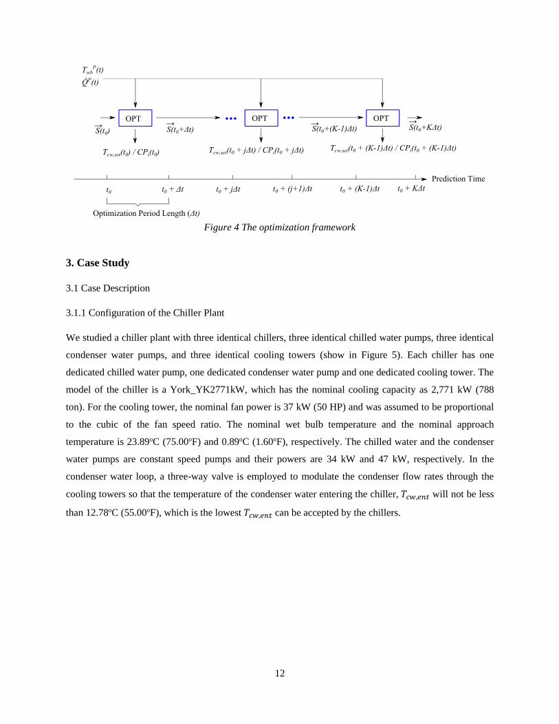
To understand when the energy saving occurred, we show the detailed analysis. As shown in Figure 7, the
chiller energy consumption was saved mainly in the summer (May to September) for Approach 1. The
cooling tower energy consumption was sometimes decreased and sometimes increased. The pump energy
consumption was increased in the summer, which indicates that the number of the operating chillers was
mainly increased to achieve an optimal load distribution. The total energy consumption was decreased
mainly in the summer. However, at a very few days, the total energy consumption was even increased.
The explanation is that the initial values of the state vectors (such as the chiller operating status) were
different from that in the baseline at these days. Thus, it is possible that Approach 1 may generate higher
total energy consumption. For example, in October 27, there were two chillers operating at the beginning
for Approach 1 while there was only one for the baseline. The total energy consumption increased for
Approach 1 compared with the baseline is around 0.2%.
Page 16
16
Figure 7 Daily energy saving by Approach 1
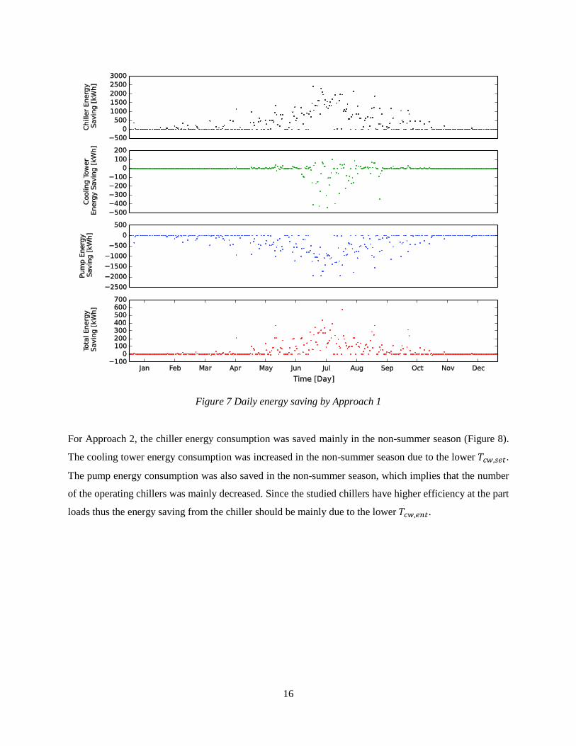
For Approach 2, the chiller energy consumption was saved mainly in the non-summer season (Figure 8).
The cooling tower energy consumption was increased in the non-summer season due to the lower 𝑇𝑐𝑤,𝑠𝑒𝑡.
The pump energy consumption was also saved in the non-summer season, which implies that the number
of the operating chillers was mainly decreased. Since the studied chillers have higher efficiency at the part
loads thus the energy saving from the chiller should be mainly due to the lower 𝑇𝑐𝑤,𝑒𝑛𝑡.
Page 17
17
Figure 8 Daily energy saving by Approach 2
As shown in Figure 9, the chiller energy consumption was saved for the most of time in the studied year
for Approach 3, which could be attributed to both the optimal load distribution and the lower 𝑇𝑐𝑤,𝑒𝑛𝑡. The
cooling tower energy consumption was mostly increased. It is also interesting to see that cooling tower
energy consumption was reduced sometimes in the summer. The pump energy consumption was
increased or reduced around the year. In the summer, the pump energy consumption was usually
increased which indicates that more chillers were operating compared with the baseline. In the rest time,
the pump energy consumption was reduced which means the cooling load was met with less chillers.
Page 18
18
Figure 9 Daily energy saving by Approach 3
Based on the above analysis, we could find that:
Approach 1’s energy savings from chillers was mostly offset by the increased energy used by the
pumps. This means that the optimal load distribution approach should be performed on chiller
plants with high efficiency condenser water pumps and high efficiency chilled water pumps.
Approach 2 can save the pump energy for about 2.0% and the chiller energy use for about 8.6%.
The pump energy use decreased because of the reducing number of the operating chillers while
the chiller energy use saving was mainly due to the lower temperature of the condenser water
entering the chiller.
Approach 3 can increase the energy saving by combining the previous two approaches, but the
total energy saving is less than the summation of their savings. Approach 3 can save the energy
used by the chillers, the cooling towers as well as the pumps. In the summer, it increased the
number of the operating chillers to save energy for the chillers and the cooling towers. In the non-
Page 19
19
summer season, it reduced the operating chiller number so that the pump energy saving can be
obtained.
3.2.1 Typical Days
In order to further identify how energy saving for different components was achieve at different seasons,
we analyzed the performance of Approach 3 for one non-summer day and one summer day. As shown in
Figure 10, the cooling load in the non-summer day (April 9) ranged from around 400 ton to 800 ton and
the wet bulb temperature was within the range from around 5oC to 10oC. The optimal 𝐶𝑃1 and 𝐶𝑃2
predicted by Approach 3 were 867 ton and 1,418 ton while the optimal 𝑇𝑐𝑤,𝑠𝑒𝑡 was 13.89oC. Since the
cooling load was always lower than 817 ton, there was only one chiller operating for Approach 3.
However, for the baseline, since the cooling load was larger than 759 ton at around 13:00, the number of
the operating chillers increased to 2 accordingly and then decreased to 1 around 17:00 when the cooling
load was less than 659 ton. There was almost no deviation of 𝑇𝑐ℎ𝑤,𝑙𝑒𝑎 from 𝑇𝑐ℎ𝑤,𝑠𝑒𝑡 for both Approach 3
and the baseline.
Figure 10 Simulated system statuses for a non-summer day
Page 20
20
As shown in Figure 11, the hourly chiller energy consumption by Approach 3 is significantly less than the
baseline over the day since the chiller is more efficient with a cooler condenser water achieved by
lowering the 𝑇𝑐𝑤,𝑠𝑒𝑡. However, having a lower 𝑇𝑐𝑤,𝑠𝑒𝑡 significantly increased the cooling tower energy
consumption. The pump energy was the same for Approach 3 as that for the baseline except the period
when there was two operating chillers for the baseline. Since the chiller energy consumption and the
pump energy consumption dominate the chiller plant energy consumption, Approach 3 always required
less energy consumption than the baseline.
Figure 11 Simulated energy consumptions for a non-summer day
As shown in Figure 12, the cooling load in the summer day (July 20) ranged from around 1,000 ton to
1,500 ton and the wet bulb temperature was within the range from around 20 to 25oC. The
optimal 𝐶𝑃1 and 𝐶𝑃2 predicted by Approach 3 were 709 ton and 1,182 ton compared to the baseline value
of 709 ton and 1,418 ton. The optimal 𝑇𝑐𝑤,𝑠𝑒𝑡 predicted by Approach 3 was 23.89oC which was the same
as the baseline. At the beginning, there were three chillers operating for Approach 3. The cooling load
decreased to be less than 1,132 ton at around 19:00 and one of the operating chillers was turned off. For
the baseline, the number of the operating chillers was two at the beginning and then turned to three at
Page 21
21
around 14:00. At around 15:30, it turned back to two. No significant deviation of 𝑇𝑐ℎ𝑤,𝑙𝑒𝑎 from 𝑇𝑐ℎ𝑤,𝑠𝑒𝑡
for both Approach 3 and the baseline was observed.
Figure 12 Simulated system statuses for a summer day
As shown in Figure 13, the hourly chiller consumption for Approach 3 was significantly less than that for
the baseline mostly because the chillers are more efficient at lower PLRs enabled by an additional chiller.
When the number of the operating chillers was the same (e.g. 20:00-24:00), the chiller energy were the
same for both Approach 3 and the baseline.
The cooling tower energy consumption was smaller for Approach 3 than that for the baseline for most of
the day since running three towers at lower speed is more energy efficient than running two towers at a
higher speed. However, in the period from 14:00 to 16:00, the cooling tower energy consumption for the
baseline was smaller. The reason is that at this period, the wet bulb temperature was relatively higher and
the cooling towers were not able to maintain 𝑇𝑐𝑤,𝑒𝑛𝑡 as the set point. In that case, adding the number of
the operating cooling towers would not affect the load ratio of each cooling tower (always be full load)
and thus the cooling tower energy consumption was increased as a result.
Page 22
22
The pump energy was mostly higher for Approach 3 than that for the baseline because additional pumps
was running for the additional chiller. However, the total energy consumption for Approach 3 was smaller
than that in the baseline for the most time of the day because the energy saving from the chillers and the
cooling towers can offset the additional energy consumption by the pumps.
Figure 13 Simulated energy consumptions for a summer day
4. Conclusion
In this study, we proposed three new CLC optimization approaches to enhance the CLC. Approach 1 is to
optimize the load distribution by adjusting the CPs. Approach 2 is to optimize the number of the
operating chillers by modulating the CPs and the condenser water set point. Approach 3 is the
combination of the first two approaches. The results suggest that the three approaches for optimizing the
chiller sequencing control can all result in energy savings with little risk. The results also suggest that one
needs to look at both the energy savings in the chillers as well as the increased energy used of other
components of the chiller plant in the chiller sequencing control optimization. Among the three
approaches, Approach 3 achieved the highest energy saving because it considered the trade-off among the
energy consumption by the chillers, the cooling towers and the pumps. In the summer, we can make more
Page 23
23
chillers operating to achieve higher energy efficiency for the chillers and the cooling towers. In the non-
summer season, we can reduce the number of the operating chillers to save the pump energy consumption.
The new CLC optimization approaches can be directly implemented in the real chiller plant for resetting
the CPs and/or the condenser water set point. They can also be used as references to help the operators
manually adjust the chiller sequencing control.
It should be noted that the evaluation of the three approaches was limited to the application in the chiller
plants with a constant primary chilled water flow rate and identical chillers in this study. In future study,
we can assess the performance of three approaches for chiller plants with variable primary chilled water
flow rates and non-identical chillers.
Acknowledgement
This research was supported by the U.S. Department of Defense under the ESTCP program. The authors
thank Marco Bonvini, Michael Wetter, Mary Ann Piette, Jessica Granderson, Oren Schetrit, Rong Lily
Hu and Guanjing Lin for the support provided through the research.
This research also emerged from the Annex 60 project, an international project conducted under the
umbrella of the International Energy Agency (IEA) within the Energy in Buildings and Communities
(EBC) Programme. Annex 60 will develop and demonstrate new-generation computational tools for
building and community energy systems based on Modelica, Functional Mockup Interface and BIM
standards.
Reference
[1] U.S. Department of Energy. Buildings Energy Data Book. <https://catalog.data.gov/dataset/buildings-
energy-data-book> (accessed May 15. 2014).
[2] Westphalen D, Koszalinski S. Energy Consumption Characteristics of Commercial Building HVAC
Systems Volume I : Chillers, Refrigerant Compressors,and Heating Systems. Arthur D. Little, Inc.; 2001.
[3] Braun JE, Diderrich GT. Near-optimal Control of Cooling Towers for Chilled-water Systems.
ASHRAE Trans 1990;96(2):806-16.
[4] Chang CC, Shieh SS, Jang SS, Wu CW, Tsou Y. Energy Conservation Improvement and ON–OFF
Switch Times Reduction for An Existing VFD-fan-based Cooling Tower. Appl Energ
2015;154(2015):491-9.
Page 24
24
[5] Chang YC. A Novel Energy Conservation Method - Optimal Chiller Loading. Electr Pow Syst Res
2004;69(2-3):221-6.
[6] Yu FW, Chan KT. Optimum Load Sharing Strategy for Multiple-chiller Systems Serving Air-
conditioned Buildings. Build Environ 2007;42(4):1581–93.
[7] Lee WS, Lin LC. Optimal Chiller Loading by Particle Swarm Algorithm for Reducing Energy
Consumption. Appl Therm Eng 2009;29(8-9):1730–4.
[8] Chua KJ, Chou SK, Yang WM, Yan J. Achieving Better Energy-efficient Air Conditioning – a
Review of Technologies and Strategies. Appl Energ 2013;104(2013):87-104.
[9] Li Z, Huang G, Sun Y. Stochastic Chiller Sequencing Control. Energ Buildings 2014;84(2014):203-13.
[10] Lu L, Cai W, Soh YC, Xie L, Li S. HVAC System Optimization - Condenser Water Loop. Energ
Convers Manage 2004;45(4):613-30.
[11] Ma Z, Wang S, Xu X, Xia F. A Supervisory Control Strategy for Building Cooling Water Systems
for Practical and Real Time Applications. Energ Convers Manage 2008;49(8):2324-36.
[12] Lee KP, Cheng TA. A Simulation–optimization Approach for Energy Efficiency of Chilled Water
System. Energ Buildings 2012;54(2012):290-6.
[13] Huang S, Zuo W. Optimization of the Water-cooled Chiller Plant System Operation. In: Proceedings
of ASHRAE/IBPSA-USA Building Simulation Conference, Atlanta, GA, U.S.A., 2014. p. 300-7.
[14] Sun J, Reddy A. Optimal Control of Building HVAC&R Systems using Complete Simulation-based
Sequential Quadratic Programming (CSB-SQP). Build Environ 2005;40(5):657-69.
[15] Yu FW, Chan KT. Optimization of Water-cooled Chiller System with Load-based Speed Control.
Appl Energ 2008;85(2008):931-50.
[16] Zhang Z, Li H, Turner WD, Deng S. Optimization of the Cooling Tower Condenser Water Leaving
Temperature using a Component-based Model. ASHRAE Trans 2011;117(1):934-44.
[17] A.Tirmizi S, P.Gandhidasan, M.Zubair S. Performance Analysis of a Chilled Water System with
Various Pumping Schemes. Appl Energ 2012;100(2012):238-48.
[18] Ma Z, Wang S. Supervisory and Optimal Control of Central Chiller Plants using Simplified Adaptive
Models and Genetic Algorithm. Appl Energ 2011;88(1):198-211.
[19] Ma Z, Wang S, Xiao F. Online Performance Evaluation of Alternative Control Strategies for
Building Cooling Water Systems Prior to In Situ Implementation. Appl Energ 2009;86(2009):712-21.
[20] Sun Y, Wang S, Huang G. Chiller Sequencing Control with Enhanced Robustness for Energy
Efficient Operation. Energ Buildings 2009;41(11):1246-55.
[21] Sun Y, Wang S, Xiao F. In Situ Performance Comparison and Evaluation of Three Chiller
Sequencing Control Strategies in a Super High-rise Building. Energ Buildings 2013;61(2013):333-43.
Page 25
25
[22] Chang YC, Lin FA, Lin CH. Optimal Chiller Sequencing by Branch and Bound Method for Saving
Energy. Energ Convers Manage 2005;46(13-14):2158-72.
[23] Chang YC, Lin JK, Chuang MH. Optimal Chiller Loading by Genetic Algorithm for Reducing
Energy Consumption. Energ Buildings 2005;37(2):147–55.
[24] Chang YC. An Outstanding Method for Saving Energy - Optimal Chiller Operation. IEEE Trans
Energy Convers 2006;21(2):527-32.
[25] Chang YC. An Innovative Approach for Demand Side Management—Optimal Chiller Loading by
Simulated Annealing. Energ 2007;31(12):1883–96.
[26] Ardakani AJ, Ardakani FF, Hosseinian SH. A Novel Approach for Optimal Chiller Loading using
Particle Swarm Optimization. Energ Buildings 2008;40(12):2177–87.
[27] Chang YC, Lee CY, Chen CR, Chou CH, Chen WH, Chen WH. Evolution Strategy based Optimal
Chiller Loading for Saving Energy. Energ Convers Manage 2009;50(1):132–9.
[28] Fan B, Jin X, Du Z. Optimal Control Strategies for Multi-chiller System based on Probability
Density Distribution of Cooling Load Ratio. Energ Buildings 2011;43(10):2813-21.
[29] Geem ZW. Solution Quality Improvement in Chiller Loading Optimization. Appl Therm Eng
2011;31(10):1848-51.
[30] Chen CL, Chang YC, Chan TS. Applying Smart Models for Energy Saving in Optimal Chiller
Loading. Energ Buildings 2014;68 Part A(2014):364-71.
[31] Coelho LdS, Mariani VC. Improved Firefly Algorithm Approach Applied to Chiller Loading for
Energy Conservation. Energ Buildings 2013;59(2013):273–8.
[32] Coelho LdS, Klein CE, Sabat SL, Mariani VC. Optimal Chiller Loading for Energy Conservation
using a New Differential Cuckoo Search Approach. Energ 2014;75(2014):237-43.
[33] Chang YC. Optimal Chiller Loading by Evolution Strategy for Saving Energy. Energ Buildings
2007;39(4):437–44.
[34] Abou-Ziyan HZ, Alajmi AF. Effect of Load-sharing Operation Strategy on the Aggregate
Performance of Existed Multiple-chiller Systems. Appl Energ 2014;135(2014):329-38.
[35] Yu KW, Chan KT. Improved Energy Management of Chiller Systems by Multivariate and Data
Envelopment Analyses. Appl Energ 2012;92(2012):168-74.
[36] Lee WL, Lee SH. Developing a Simplified Model for Evaluating Chiller-system Configurations.
Appl Energ 2007;84(2007):290-306.
[37] Tirmizi SA, Gandhidasan P, Zubair SM. Performance Analysis of a Chilled Water System with
Various Pumping Schemes. Appl Energ 2012;100(2012):238-48.
Page 26
26
[38] Myat A, Choon NK, Thu K, Kim YD. Experimental Investigation on the Optimal Performance of
Zeolite–water Adsorption Chiller. Appl Energ 2013;102(2013):582-90.
[39] Liao Y, Huang G, Sun Y, Zhang L. Uncertainty Analysis for Chiller Sequencing Control. Energ
Buildings 2014;85(2014):187-98.
[40] F.W. Yu, Chan KT. Improved Energy Performance of Air Cooled Centrifugal Chillers with Variable
Chilled Water Flow. Energ Convers Manage 2008;49(6):1595–611.
[41] Chang YC, Chen WH, Lee CY, Huang CN. Simulated Annealing Based Optimal Chiller Loading for
Saving Energy. Energ Convers Manage 2006;47(15-16):2044-58.
[42] Chang YC, Chen WH. Optimal Chilled Water Temperture Calculation of Mutiple Chiller Systems
using Hopfield Neural Network for Saving Energy. Energ 2008;34(4):448-56.
[43] Lu YY, Chen JH, Liu TC, Chien MH. Using Cooling Load Forecast as the Optimal Operation
Scheme for a Large Multi-chiller System. Int J Refrig 2011;34(8):2050–62.
[44] ASHRAE. ASHRAE Handbook HVAC Application. Atlanta: ASHRAE, Inc.; 2011.
[45] Honeywell. Engineering Manual of Automatic Control for Commercial Buildings. Minneapolis:
Honeywell, Inc.; 1997.
[46] Kent A, Williams JG. Encyclopedia of Computer Science and Technology: Volume 25 - Supplement
10: Applications of Artificial Intelligence to Agriculture and Natural Resource Management to
Transaction Machine. New York: Marcek Dekker, Inc.; 1991.
[47] Crawley DB, Lawrie LK, Winkelmann FC, Buhl WF, Huang YJ, Pedersend CO, et al. EnergyPlus:
Creating a New-generation Building Energy Simulation Program. Energ Buildings 2001;33(4):319-31.
[48] Boyd SP, Vandenberghe L. Convex Optimization. New York: Cambridge University Press; 2004.
[49] Wetter M, Zuo W, Nouidui T, Pang X. Modelica Buildings library. J Build Perform Simu
2014;7(4):253-70.
[50] Nouidui TS, Phalak K, Zuo W, Wetter M. Validation of the Window Model of the Modelica
Buildings Library. In: Proceedings of the 9th International Modelica Conference, Munich, Germany, 2012.
p. 727-36.
[51] Zuo W, Wetter M, Li D, Jin M, Tian W, Chen Q. Coupled Simulation of Indoor Enviroment, HVAC
and Control System by using Fast Fluid Dynamics and the Modelica Buildings Library. In: Proceedings
of ASHRAE/IBPSA-USA Building Simulation Conference, Atlanta, GA, U.S.A., 2014. p. 56-63.
[52] Otter M, Årzén K-E, Dressler I. StateGraph - a Modelica Library for Hierarchical State Machines. In:
Proceedings of the 4th International Modelica Conference, Hamburg, Germany, 2005. p. 569-78.
[53] Huang S, Zuo W, Sohn MD. A New Method for the Optimal Chiller Sequencing Control. In:
Proceedings of the 14th Conference of IBPSA, Hyderabad, India, 2015.
Page 27
27
[54] Hooke R, Jeeves TA. ''Direct Search'' Solution of Numerical and Statistical Problems. J ACM
1961;8(2):212-29.
[55] Wetter M. GenOpt - a Generic Optimization Program. In: Proceedings of the 7th IBPSA Conference,
Rio de Janeiro, Brazil, 2001. p. 601-8.
[56] National Climatic Data Center. Quality Controlled Local Climatological Data.
<http://www.ncdc.noaa.gov/data-access/land-based-station-data/land-based-datasets/quality-controlled-
local-climatological-data-qclcd> (accessed May 14. 2015).