American Finance Association

On the Existence of an Optimal Capital Structure: Theory and EvidenceAuthor(s): Michael Bradley, Gregg A. Jarrell, E. Han KimSource: The Journal of Finance, Vol. 39, No. 3, Papers and Proceedings, Forty-Second AnnualMeeting, American Finance Association, San Francisco, CA, December 28-30, 1983 (Jul., 1984),pp. 857-878Published by: Blackwell Publishing for the American Finance AssociationStable URL: http://www.jstor.org/stable/2327950Accessed: 22/01/2009 14:04

Your use of the JSTOR archive indicates your acceptance of JSTOR's Terms and Conditions of Use, available athttp://www.jstor.org/page/info/about/policies/terms.jsp. JSTOR's Terms and Conditions of Use provides, in part, that unlessyou have obtained prior permission, you may not download an entire issue of a journal or multiple copies of articles, and youmay use content in the JSTOR archive only for your personal, non-commercial use.

Please contact the publisher regarding any further use of this work. Publisher contact information may be obtained athttp://www.jstor.org/action/showPublisher?publisherCode=black.

Each copy of any part of a JSTOR transmission must contain the same copyright notice that appears on the screen or printedpage of such transmission.

JSTOR is a not-for-profit organization founded in 1995 to build trusted digital archives for scholarship. We work with thescholarly community to preserve their work and the materials they rely upon, and to build a common research platform thatpromotes the discovery and use of these resources. For more information about JSTOR, please contact support@jstor.org.

Blackwell Publishing and American Finance Association are collaborating with JSTOR to digitize, preserveand extend access to The Journal of Finance.

http://www.jstor.org

THE JOURNAL OF FINANCE * VOL. XXXIX, NO. 3 * JULY 1984

On the Existence of an Optimal Capital Structure: Theory and Evidence

MICHAEL BRADLEY, GREGG A. JARRELL, and E. HAN KIM*

ONE OF THE MOST contentious issues in the theory of finance during the past quarter century has been the theory of capital structure. The geneses of this controversy were the seminal contributions by Modigliani and Miller [18, 19]. The general academic view by the mid-1970s, although not a consensus, was that the optimal capital structure involves balancing the tax advantage of debt against the present value of bankruptcy costs. No sooner did this general view become prevalent in the profession than Miller [16] presented a new challenge by showing that under certain conditions the tax advantage of debt financing at the firm level is exactly offset by the tax disadvantage of debt at the personal level. Since then there has developed a burgeoning theoretical literature attempting to reconcile Miller's model with the balancing theory of optimal capital structure [e.g., DeAngelo and Masulis [5], Kim [12], and Modigliani [17]. The general result of this work is that if there are significant "leverage-related" costs, such as bankruptcy costs, agency costs of debt, and loss of non-debt tax shields, and if the income from equity is untaxed, then the marginal bondholder's tax rate will be less than the corporate rate and there will be a positive net tax advantage to corporate debt financing. The firm's optimal capital structure will involve the trade off between the tax advantage of debt and various leverage-related costs. The upshot of these extensions of Miller's model is the recognition that the existence of an optimal capital structure is essentially an empirical issue as to whether or not the various leverage-related costs are economically significant enough to influence the costs of corporate borrowing.

The Miller model and its theoretical extensions have inspired several time- series studies which provide evidence on the existence of leverage-related costs. Trczinka [28] reports that from examining differences in average yields between taxable corporate bonds and tax-exempt municipal bonds, one cannot reject the Miller hypothesis that the marginal bondholder's tax rate is not different from the corporate tax rate. However, Trczinka is careful to point out that this finding does not necessarily imply that there is no tax advantage of corporate debt if the personal tax rate on equity is positive. Indeed, Buser and Hess [1], using a longer time series of data and more sophisticated econometric techniques, estimate that the average effective personal tax rate on equity is statistically positive and is not of a trivial magnitude. More importantly, they document evidence that is consistent with the existence of significant leverage-related costs in the economy.

* The University of Michigan, Lexecon Inc., and The University of Michigan, respectively. This research was supported by summer research grants from the University of Michigan Graduate School of Business Administration.

857

858 The Journal of Finance

Their results show that leverage-related costs and the tax rate on equity have important impacts on the relation between taxable and tax-exempt yields. These findings of Buser and Hess are further buttressed by Trzcinka and Kamma [29] who find that the marginal bondholder's tax rate is significantly less than the corporate rate. They conclude that the extensions of Miller's model with positive leverage-related costs describe the data better than the original Miller model.

In this study we take a more direct approach to the issue of an optimal capital structure. In contrast to the above studies that are based on time-series analyses of macrodata, we use cross-sectional, firm-specific data to test for the existence of an optimal capital structure.' Thus, the evidence provided in this study may be viewed as a complementary to the above time-series evidence.2

Section I develops a theoretical model that synthesizes the recent advances in the theory of optimal capital structure. Section II presents testable implications of the theory by using comparative statics and a simulation of the model. The simulation shows that firm leverage ratios will be negatively related to the volatility of firm earnings if the costs of financial distress (bankruptcy costs and agency costs of debt) are non-trivial.

In Section III we examine the cross-sectional variations in firm leverage ratios to see if they are related to 1) the through-time volatility of firm earnings, 2) the relative amount of non-debt tax shields (depreciation and tax credits), and 3) the intensity of research and development and advertising expenditures. We focus on a 20-year average debt-to-value measure, to minimize the effects of transient variations through time because of business cycles or lagged adjust- ments by firms towards their "target" leverage ratios. We find that the "perma- nent" or average firm leverage ratios are strongly related to industry classifica- tion, and that this relation remains strong even after we exclude regulated firms. More important, we find firm leverage ratios are related inversely to earnings volatility. These results are consistent with the theory of optimal capital struc- ture.

L A Model of Optimal Capital Structure

In this section we develop a single period model that synthesizes the current state of the art in the theory of optimal capital structure. The model captures the essence of the tax-advantage-and-bankruptcy-costs trade off models of Kraus and Litzenberger [14], Scott [24], Kim [11], and Titman [27], the agency costs of debt arguments of Jensen and Meckling [10] and Myers [20], the potential loss of non-debt tax shields in non-default states in DeAngelo and Masulis [5],

1 Other recent empirical studies of optimal capital structure that are based on cross-sectional, firm- specific data include [6], [7], [15], [3], [2], and [26]. In contrast to the concensus among the authors who have examined the differential yields between taxable and tax-exempt bonds, these authors reach quite different conclusions on the existence of an optimal capital structure. This lack of concensus reflects the fact that these authors use different methodologies and samples.

2Another empirical implication of Miller's model is that shareholders will sort themselves into leverage clienteles depending upon their tax rates relative to the corporate tax rate. Kim, Lewellen, and McConnell [13] develop this implication of Miller's model and provide some preliminary evidence. Harris, Roenfeldt, and Cooley [9] provide further evidence on the existence of shareholder leverage clienteles.

Theory and Evidence 859

the differential personal tax rates between income from stocks and bonds in Miller [16], and the extensions of Miller's model by DeAngelo and Masulis [5], Kim [12], and Modigliani [17].

To develop a model that represents the current state of the art in the theory of optimal capital structure, we make the following assumptions.

1. Investors are risk-neutral. 2. Investors face a progressive tax rate on returns from bonds, tpb, while the

firm faces a constant statutory marginal tax rate, tc. 3. Corporate and personal taxes are based on end-of-period wealth; conse-

quently, debt payments (interest and principle) are fully deductable in calculating the firm's end-of-period tax bill, and are fully taxable at the level of the individual bondholder.

4. Equity returns (dividends and capital gains) are taxed at a constant rate, tps.

5. There exist non-debt tax shields, such as accelerated depreciation and investment tax credits, that reduce the firm's end-of-period tax liability.

6. Negative tax bills (unused tax credits) are not transferrable (saleable) either through time or across firms.

7. The firm will incur various costs associated with financial distress should it fail to meet, in full, the end-of-period payment promised to its bondholders.

8. The firm's end-of-period value before taxes and debt payments, X, is a random variable. If the firm fails to meet the debt obligation to its bond- holders, Y, the costs associated with financial distress will reduce the value of the firm by a constant fraction k.

Assumption 1, that of risk neutrality, eliminates the need to model the general equilibrium issue of the trade-off between the tax status and the risk/expected return characteristic of debt and equity securities (e.g., Kim [12] and Modigliani [17]). In this context, risk-neutrality is equivalent to assuming that investors form either all-equity or all-debt portfolios depending on their tax rates.

Assumptions 2 through 4 describe the tax environment of the model. Assump- tion 2 originates with Miller [16], while Assumption 3, that of wealth tax, has been used by a number of authors to capture the spirit of a perpetuity analysis in a single period framework (e.g., [14], [5], and [12]). Assumption 4 relaxes the undesirable assumption of a zero tax rate on income from stocks that has been commonly used by previous authors.

Assumptions 5 and 6 are made to incorporate the effects of non-debt tax shields on the corporate leverage decision. Assumption 6 prohibits firms from carrying tax credits backward or forward, or from selling them via a leasing agreement or through a merger. While this assumption is admittedly too restric- tive, the purpose is to capture DeAngelo and Masulis' [5] argument that the possibility of losing non-debt tax shields in non-default states creates a substi- tution effect between the level of non-debt tax shields and the tax benefits of corporate leverage.

Finally, Assumptions 7 and 8 allow for the existence of costs associated with risky debt that are incurred when the firm encounters difficulty in meeting its end-of-period obligation to its debtholders. In the agency costs framework of Jensen and Meckling [10] and Myers [20], these costs include the costs of

860 The Journal of Finance

renegotiating the firm's debt contracts and the opportunity costs of non-optimal production/investment decisions that arise when the firm is in financial distress. In the bankruptcy cost framework of Kraus and Litzenberger [14], Scott [24], Kim [11], and Titman [27], these costs represent the direct and indirect costs of bankruptcy. Since both the agency costs of debt and bankruptcy costs become economically significant only when the firm is in financial distress we use the term "costs of financial distress" in a generic sense to include both bankruptcy and agency costs of debt. The costs of financial distress are assumed to be a constant fraction k of X, the firm's end-of-period value before taxes, in the event of financial distress, and zero otherwise.

Under the above assumptions of the model, the uncertain end-of-period pre- tax returns to the firm's stockholders and bondholders can be written as follows:

((X - Y)( - tc) + X, X >. Y + 01tc Ys = X- Y, Ys <X < Y + 40/tc (1)

0o, X< Y

(Y, Xo .YA

Yb={X(l-k), 0sX< Y (2) 0, X < O,

where

Ys, Yb = the gross end-of-period returns to stockholders and bondholders, respectively,

Y = the total end-of-period promised payment to bondholders, 10 = the total after-tax value of the non-debt shields if they are fully

utilized at the end-of-period, k = costs of financial distress per dollar of end-of-period value of the

firm.

Equation (1) shows that if pre-tax earnings are large enough for the firm to fully utilize the non-debt tax shield (l/t,), then the gross end-of-period return to stockholders is (X - Y - /tc)(1- tc) + l/tc = (X - Y)(1 - tc) + 4. If the firm's pre-tax earnings are such that X - Y - '/tc < 0, the firm will pay no tax and Assumption 6 implies that the end-of-period return to stockholders is X - Y. The end-of-period pre-tax return to bondholders in Equation (2) follows from Assumption 8 and the fact that bondholders have limited liability in the event that the firm's end-of-period value X is negative.

Invoking Assumption 1, that of risk neutrality, Equations (1) and (2) provide the following beginning-of-period market value of the firm's stocks (S) and bonds (B):

8= E(Y6/E(S) rO 1Y+tc [(X - )(1 Ct) + 0]f(X) dX

rY+Oltc + (X - Y)f(X) dX (3)

B = E(Yb)/E(Qb) = 1 p6 Yf (X) dX + f X(1 - k)f (X) dXi, (4)

Theory and Evidence 861 where

S, B = the market value of the firm's stocks and bonds, respectively, E(?8), E(Qb) = one plus the expected pre-tax rate of return from stocks and

bonds, respectively, ro = one plus the rate of return on default-free, tax-exempt bonds,

f (X) = probability density of X.

Adding Equations (3) and (4) yields the market value of the firm (V):

V= [(1 - tpb) ( X(- k)f (X) dX

rY+Oltc

+ f [(X - Y)(1 - tps) + Y(- tpb)]f(X) dX

+ js [(1 - - iX Y)(1-tc) + '} + (1 -tb)Y]f(X) dXl (5)

Equation (5) shows that the value of the firm is equal to the present value of the sum of three expected values (integrals). The first integral represents the situation in which X is positive but insufficient to meet its debt obligation. Under this condition, the payment to the firm's bondholders is X less total costs of financial distress, kX. Consistent with the assumption of a wealth tax, the payment to the firm's bondholders, net of costs of financial distress, is subject to the personal tax rate tpb. The second integral represents the states of world in which the firm's end-of-period pre-tax value, X, is greater than its debt obligation (Y) but less than the maximum level of earnings that would result in a zero end- of-period corporate tax bill (Y + l/tc). In these states, the firm has no corporate tax bill; however, the payments to bondholders and stockholders are subject to the personal tax rates. Finally, the third integral defines the after-tax cash flows to the firm's securityholders if earnings are sufficient to pay bondholders and to generate a positive corporate tax liability.

The firm's optimal leverage decision involves setting Y, the end-of-period payment promised to bondholders, such that the market value of the firm is maximized. Differentiating (5) with respect to Y yields the first order condition of Equation (6), where Vv is the partial derivative a V/8 Y.

rO t1 -h [ 1-tpb J

-(1-t,,,jz [F (Y + l/tc) -F(Y)] -kYf (Y)}* (6)

where F (*) is the cumulative probability density function of X. To explain the implications of Equation (6), we use it to illustrate the existing

theories of capital structure. The Miller irrelevancy model [16] assumes no tax on income from stocks and no leverage-related costs, i.e., tp = k = =O, which reduce (6) to:

Vk = l - F(YY)]tc - [1 - F(Y)]tpbl/ro (7)

862 The Journal of Finance

The first term in Equation (7) is the marginal expected tax benefit of debt, while the second term is the marginal tax premium firms expect to pay bondholders. When debt is risky, the marginal expected tax benefit of debt is the corporate tax rate (tc) times the probability that the firm will keep its promise to the bondholders [1 -F(Y)]. Equation (7) shows that firms will issue debt up to the point where the marginal tax premium they expect to pay bondholders, [1 - F(Y)] tpb, is equal to the marginal expected tax benefit of debt, [1 - F(Y)]tc. Firms in the economy will continue to issue debt until, due to the progressivity of the personal tax schedule, tpb equals tc. Thus, in equilibrium the net tax advantage of debt is zero.

Alternatively, DeAngelo and Masulis [5] and Kim [12], while retaining the assumption of no personal tax on income from stocks (tp = 0), allow for positive leverage-related costs. In this case, (6) becomes

Vy = f[l - F(Y)](tc - tpb) - tc[F(Y + 40/tc)

- F(Y)] - (1 -tpb)kYf (Y)/ro (8)

Equation (8) now shows that firms will stop issuing debt when

tc - tpb = ttc[F(Y + 4/tc) - F(Y)] + (1 - tpb)kYf(Y)1/[1 - F(Y)]. (9)

Note that as long as either 0 or k is positive, the RHS of Equation (9) is unambiguously positive and hence t, is greater than tpb. That is, firms will stop issuing debt while the marginal bondholder's tpb is less than tc. Thus, in equilib- rium the first term in Equation (8) is positive, which means that the net tax advantage of debt is positive. The second and third terms define the marginal cost of debt. The second term represents the increase in the probability of wasting interest tax shields in states where the nondebt tax shields are greater than taxable earnings. The third term represents the marginal increase in expected costs of financial distress. Thus, the firm's leverage decision involves a tradeoff between the expected net tax advantage of debt and expected leverage-related costs.

Finally, if we allow for a positive personal tax rate on income from stocks (tpS > 0), Equation (6) shows that the tax terms become more complicated; however, the essence of the results obtained by DeAngelo and Masulis and Kim does not change. The first term in (6) represents the marginal net tax advantage of debt, while the second and third terms represent marginal expected leverage-related costs. The optimal leverage involves balancing the net tax advantage of debt against leverage-related costs.

To show that the net tax advantage of debt is positive with a positive tp,, consider both the demand and supply of corporate debt and equity. In a risk neutral world, investors are indifferent between holding stocks and bonds as long as the expected after-tax returns are the same:

E(r*)(1 - tps) = E(Pb)(1 - tpb)- (10)

On the corporate side, firms are indifferent between issuing stocks and bonds as long as the marginal expected after-tax cost of issuing debt is the same as the

Theory and Evidence 863

marginal expected cost of issuing equity:

[E(r-b) + 1](1 - tc) + A = E(iQ) (11)

where I is the marginal expected costs of financial distress that firms pay in the form of higher promised interest rates and A& is the interest tax shields that are expected to be wasted due to states where non-debt tax shields are greater than taxable earnings. Since in equilibrium demand must equal supply, we substitute Equation (10) into Equation (11) and rearrange terms to obtain the equilibrium condition:

(1 - tc)(1 - tps)/(l - tpb) = [E(rb) - t(1 - tps)/(l - tb)]I/[E(rib) + 1]. (12)

Note that if either A or 1 is positive, the LHS of Equation (12) must be less than one and hence the first term in Equation (6), the net tax advantage of debt financing, must be positive.

II. Comparative Statics and Simulation of the Model

The comparative statics of the leverage relevancy model can be shown by differentiating the optimality condition (6) with respect to each of the relevant exogenous variables. Differentiating Vk in (6) with respect to k, 4, tpb, and tp, yields the following cross-partial derivatives:

Vf?k = -(1 - tpb) Yf( Y)/ro < 0 (13)

VfO = -(1 - tps)f (Y + 4/tc)/ro < 0 (14)

Vyt = f[1 - F()] - tc[l -F(Yi + k/tc)]1/ro

> (1 - tc)[1 - F(Y)]/ro > O (15)

Vft,b = Ik&f(5AY) - [1 - F(Y)]I/ro.

(16) The cross-partial derivatives in Equations (13) and (14) are unambiguously

negative. An increase in either the cost of financial distress or in non-debt tax shields will lead to a reduction in the optimal level of debt.

The cross-partial derivative in Equation (15) is unambiguously positive. An increase in the personal tax rate on equity increases the stockholder's after- personal-tax value of corporate interest tax shields and hence increases the optimal level of corporate debt. Finally, the cross-partial derivative in Equation (16) is unambiguously negative at the firm's optimal capital structure,3 An

3Substituting the optimality condition (6) into Equation (16) yields the cross-partial at the optimal capital structure:

V~-~frl~(Y*~1 (1 - t0(1 - tp,) (1Y- tpb)t4 Vfyto = 1-F(Y*)] (1 - tpo) + 1 - tpo

*[F(Y* + /t,) - F(V*)I} /rO < 0, (17)

where Y* is the optimal level of debt.

864 The Journal of Finance

increase in the marginal bondholder's tax rate decreases the optimal level of debt because it increases the tax premium component of corporate bond yields.

A factor that does not appear explicitly in the leverage optimality condition (6) but is important to the theory of optimal capital structure is the variability of the firm's end-of-period value. Intuitively, the greater the variability of the firm's value, the greater the probability of incurring costs of financial distress at the end of the period and the greater the probability of wasting interest tax shields. However, this intuitively appealing argument is not an unambiguous implication of the model. To demonstrate this ambiguity, we differentiate (6) with respect to a, the standard deviation of the distribution of the firm's end-of- period value, assuming that X is normally distributed.

V-y = {tc(1 - tps)f (Y + 01/tc) ( + ) - (tpb - tps)f(v)(y

-(1- tpb)kYf(Y) [ ro a 0, (18)

where X is the mean of X. The ambiguity of the sign of this cross-partial derivative, when the underlying distribution is normal, has been pointed out by Scott [24] and Castanias [3]. Equation (18) indicates that the sign of Vk, is determined in part by the magnitudes of Y and Y + 1/tc relative to X, and by the magnitudes of k and X relative to other variables.4

In order to establish the empirically relevant sign of the cross-partial derivative VV,q, we perform a simulation of the firm's leverage decision based on the first- order condition (6). In this simulation we assume a normal distribution for X and specific values for the relevant variables and compute the optimal level of debt Y*, which is the value that sets Vy in (6) equal to zero. Then, we compute the market value of the firm's stock at Y* using Equation (3).

The optimal debt ratio, d, is defined as Y*/(S + Y*). Note that in this definition, debt is measured by the end-of-period payment promised to the bondholders, instead of by the market value of bonds, while equity is measured by the market value of stock. The purpose here is to be consistent with our empirical proxy for the debt ratio in the cross-sectional tests, which is the book value of debt divided by the sum of the market value of equity and the book value of debt. The book value of debt is more representative of the promised payment to debtholders than is the market value of debt.

After obtaining the optimal debt ratio for a set of specific variables, the simulation changes the assumed values of a, 4, and k systematically and shows how the relation between the optimal debt ratio and a changes under different values for- 0 and k. The results from this sensitivity analysis provide the basis for interpreting the empirical results in the next section.

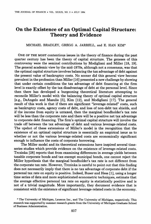
The numerical values assumed for the simulation are as follows: X = 100, f = (5 through 100) in units of 5, X = (O through 40) in units of 10, and k = (O

It is possible for the cross-partial to be positive, because beyond a certain level of Y, an increase in a will decrease the probability that X will be less than Y and/or Y + 01tc, which will in turn lead the firm to increase its Y.

Theory and Evidence 865 1. 0

0.8

10

cr.

?cl . 4 \

0~~~~~~~~2 = 20

\)=30

0. 0 \ 40 \ I

0 20 40 60 80 100 S I GMR

Figure 1. K= 0.0

through 1) in units of 0.2. The initial set of marginal tax rates assumed are: tpb

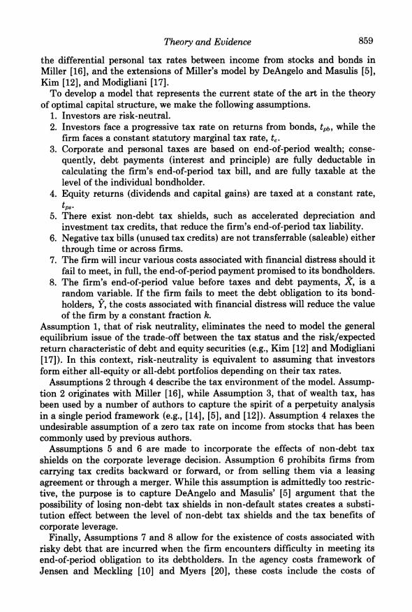
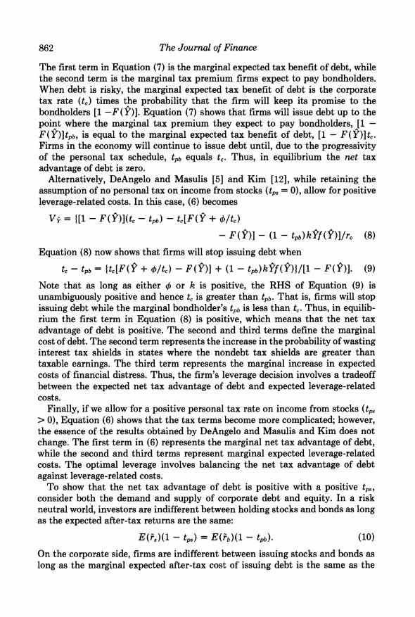
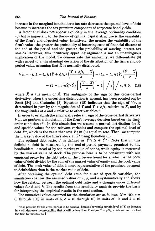
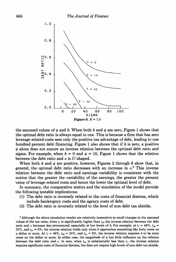
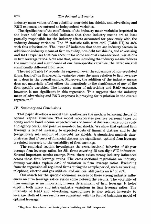
= tc = 45%, and tp, = 12%.5 Figures 1 through 6 depict the results of the simulation of the firm's optimal leverage decision. The vertical axis measures the optimal debt ratio. The horizontal axis measures different levels of a. Each line in the figures depicts the functional relation between the optimal debt ratio and the variability of the firm's value, for different levels of k and 0. There is a separate figure for each value of k, ranging from zero (Figure 1) to one (Figure 6). In each figure, five different levels of non-debt tax shields (4O from 0 to 40) generate five curves relating leverage to sigma.

As predicted by the comparative statics in (13) and (14), Figures 1 through 6 show that, for any given level of a, an increase either in the cost of financial distress (k) or in non-debt tax shields (4i) leads to a reduction in the optimal debt ratio.

Also as predicted by the cross-partial in (18), the simulation results confirm that the effect of an increase in a on the optimal debt ratio is ambiguous. Further, the functional relation between the optimal debt ratio and a changes as we vary

'This set of -tax rates is consistent with the recent empirical estimates provided by Buser and Hess [1] and by Trczinka [28]. Based on one-year T-bill rates and one-year prime, high grade municipal yields over the period of 1950 through 1982, Buser and Hess estimate the average marginal bondholder's tax rate to be 42.5%. Also during the same period they estimate that the average effective personal tax rates on equity and marginal corporate tax rates are 12% and 45%, respectively. Trczinka's estimate of the marginal bondholder's tax rate is based on monthly averages of yields of various grades and maturities during the period of 1970 through 1979. He concludes that he cannot reject the hypothesis that tpb is equal to t, of 48% but provides no estimate for the personal tax rate on income from stocks.

866 The Journal of Finance

1.0

0.8

006

cc

0O. 4 \ a:

\0\ ? = 20

0.2 = 30

0.0 . I 4

-- I I I I

0 20 40 60 80 100 S I GMR

Figure 2. K= 0.2

1.0

0. 8

0l: \ \ f = 10

m O. 4\

0.2

0 20 40 60 80 100 S I GMR

Figure 3. K = 0.4

Theory and Evidence 867

1.0

0.8

20.6

a:\ \

m 0. 4 \ 0 _

0.2 -=20

= 30 = 40

0.0 I I I I I I 0 20 40 60 80 100

S I GMR

Figure 4. K= 0.6

1.0

0. 8

a:

I-- m 0 . 4 \ =10

0.2 \=20

= 30

0.0 l \t=L40 0 20 40 60 80 100

S I GMR

Figure 5. K = 0.8

868 The Journal of Finance

1. 0

0. 8

00.6

C O . 4 \ \

0.2 .P=20

(P \= 40' 0. O I I I

0 20 40 60 80 100 S I GMA

Figure 6. K= 1.0

the assumed values of X and k. When both k and q are zero, Figure 1 shows that the optimal debt ratio is always equal to one. This is because a firm that has zero leverage-related costs sees only the positive tax advantage of debt, leading to one hundred percent debt financing. Figure 1 also shows that if k is zero, a positive X alone does not ensure an inverse relation between the optimal debt ratio and sigma. For example, when k = 0 and q = 10, Figure 1 shows that the relation between the debt ratio and a is U-shaped.

When both k and X are positive, however, Figures 2 through 6 show that, in general, the optimal debt ratio decreases with an increase in a.6 This inverse relation between the debt ratio and earnings variability is consistent with the notion that the greater the variability of the earnings, the greater the present value of leverage-related costs and hence the lower the optimal level of debt.

In summary, the comparative statics and the simulation of the model provide the following testable implications:

(1) The debt ratio is inversely related to the costs of financial distress, which include bankruptcy costs and the agency costs of debt.

(2) The debt ratio is inversely related to the level of non-debt tax shields.

6Although the above simulation results are relatively insensitive to small changes in the assumed values of the tax rates, when t, is significantly higher than t,,b the inverse relation between the debt ratio and a becomes less pronounced, especially at low levels of k. For example, at t, = 48%, tAp =

33%, and tp, = 0%, the inverse relation holds only when k approaches something like forty cents on a dollar or more. At t, = 48%, tpb = 33%, and tp8 = 9%, the inverse relation requires k to be sixty cents on the dollar or more. In either case, the magnitude of 4 has little influence on the relation between the debt ratio and a. In sum, when tpb is substantially less than t,, the inverse relation requires significant costs of financial distress, but does not require high levels of non-debt tax shields.

Theory and Evidence 869

(3) The debt ratio is inversely related to the variability of firm value, if the costs of financial distress are significant.

III. Empirical Tests and Results

The theory highlights three firm-specific factors that influence the firm's optimal capital structure: the variability of firm value, the level of non-debt tax shields, and the magnitude of the costs of financial distress. These three factors could quite plausibly also exhibit important industry commonalities. This may account for the empirical evidence that firm leverage ratios are industry related, although this result is contradicted by some studies. Schwartz and Aronson [22] and Scott [23] in particular report persistent differences across industries and strong intra-industry similarities in firm leverage ratios. However, the contrary findings by Remmers, et. al. [21], Ferri and Jones [6], and Chaplinsky [2] justify another investigation of this important empirical question. We first re-examine the cross-sectional relation between 20-year average firm leverage ratios and industrial classification with a sample of 851 firms covering 25 two-digit SIC industries. We then regress firm leverage ratios on empirical proxy variables for the three firm-specific factors in an effort to test the more direct implications of the theory of optimal capital structure.

A. Analysis of Variance of Firm Leverage Ratios by Industrial Classification

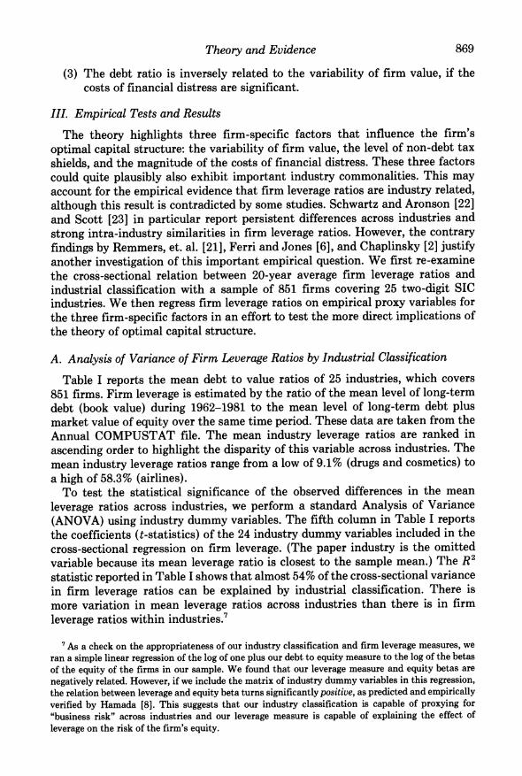
Table I reports the mean debt to value ratios of 25 industries, which covers 851 firms. Firm leverage is estimated by the ratio of the mean level of long-term debt (book value) during 1962-1981 to the mean level of long-term debt plus market value of equity over the same time period. These data are taken from the Annual COMPUSTAT file. The mean industry leverage ratios are ranked in ascending order to highlight the disparity of this variable across industries. The mean industry leverage ratios range from a low of 9.1% (drugs and cosmetics) to a high of 58.3% (airlines).

To test the statistical significance of the observed differences in the mean leverage ratios across industries, we perform a standard Analysis of Variance (ANOVA) using industry dummy variables. The fifth column in Table I reports the coefficients (t-statistics) of the 24 industry dummy variables included in the cross-sectional regression on firm leverage. (The paper industry is the omitted variable because its mean leverage ratio is closest to the sample mean.) The R2 statistic reported in Table I shows that almost 54% of the cross-sectional variance in firm leverage ratios can be explained by industrial classification. There is more variation in mean leverage ratios across industries than there is in firm leverage ratios within industries.7

7As a check on the appropriateness of our industry classification and firm leverage measures, we ran a simple linear regression of the log of one plus our debt to equity measure to the log of the betas of the equity of the firms in our sample. We found that our leverage measure and equity betas are negatively related. However, if we include the matrix of industry dummy variables in this regression, the relation between leverage and equity beta turns significantly positive, as predicted and empirically verified by Hamada [8]. This suggests that our industry classification is capable of proxying for "business risk" across industries and our leverage measure is capable of explaining the effect of leverage on the risk of the firm's equity.

870 The Journal of Finance

Table I Mean and Dummy Variable Coefficient of the Debt to Value RatiosA for 25

Industries, Ranked in Ascending Order of Mean Debt to Value Ratios. Mean Dummy Variable Coefficients

(Standard (t-statistics) Deviation)

Sic Industry Nobs Debt to Value All Firms Non-Regulated

2830, 40 Drugs and Cosmetics 31 .0907 (.095) -.199 (-5.64) -.148 (-3.21) 3800 Instruments 27 .1119 (.086) -.178 (-4.88) -.126 (-2.69) 1000 Metal Mining 23 .1347 (.099) -.155 (-4.09) -.104 (-2.15) 2700 Publishing 16 .1552 (.169) -.134 (-3.21) -.083 (-1.61) 3600 Electronics 77 .1579 (.121) -.132 (-4.34) -.080 (-1.91) 3500 Machinery 80 .1957 (.114) -.094 (-3.11) -.043 (-1.02) 2000 Food 50 .2056 (.128) -.084 (-2.60) -.033 (-0.75) 1300 Petroleum Exploration 24 .2258 (.151) -.064 (-1.70) -0.13 (-0.26) 15, 16, 1700 Construction 12 .2384 (.151) -.051 (-1.12) B

2900 - Petroleum Refining 31 .2436 (.121) -.046 (-1.30) .005 (0.11) 3400 Metal Working 33 .2502 (.139) -.039 (-1.13) .012 (0.26) 2800 Chemicals 47 .2544 (.135) -.035 (-1.08) .060 (0.36) 2300 Apparel 18 .2603 (.123) -.029 (-0.72) .022 (0.43) 2400 Lumber 7 .2605 (.182) -.029 (-0.52) .022 (0.34) 3700 Motor Vehicle Parts 52 .2714 (.138) -.018 (-0.56) .033 (0.76) 2600 Paper 24 .2895 (.114) B .051 (1.07) 2200 Textile Mill Products 21 .3257 (.133) .036 (0.93) .087 (1.78) 3000 Rubber 26 .3262 (.167) .037 (1.00) .088 (1.86) 5300 Retail Dept. Stores 20 .3433 (.150) .054 (1.37) .105 (2.12) 5400 Retail Grocery Stores 16 .3460 (.187) .056 (1.35) .108 (2.08) 4200 Trucking 10 .3730 (.209) .083 (1.71) 3300 Steel 45 .3819 (.195) .092 (2.82) .143 (3.26) 4800 Telephone 10 .5150 (.097) .226 (4.62) 4900 Elec. & Gas Utilities 135 .5309 (.081) .241 (8.40) 4500 Airlines 16 .5825 (.171) .293 (7.00)

TOTAL 851 .2913 (.188) R-SQRD .536 .248 F-STATISTIC 39.71 10.85

A Firm Debt to Value Ratio is calculated as the 20-year (1962-1981) sum of annual book value of long-term debt divided by the sum of long-term debt and the market value of equity.

B Omitted industry.

Table I contains several industries that were highly regulated by governmental agencies over the sample period of 1962 through 1981, and there appears to be a systematic relation between regulation and financial leverage. Regulated firms such as telephone, electric and gas utilities, and airlines are consistently among the most highly levered firms, which raises the possibility that differences between regulated and unregulated firm leverage ratios (for whatever reasons) are primarily responsible for the overall ANOVA results. Thus, we rerun the ANOVA of firm leverage excluding firms in the regulated industries.

The sixth column in Table I reports the coefficient (t-statistics) of the dummy variables of the ANOVA for non-regulated firms. While both the R2 and F- statistics fall with the exclusion of the regulated industries, industry classification still accounts for almost 25% of the cross-sectional variation in firm leverage. In

Theory and Evidence 871

sum, a regulatory effect is evident in the data, but there still exist significant differences in the mean leverage ratios of firms across non-regulated industries.8

B. Empirical Proxies

Although our confirmation of a systematic relation between the debt ratio and industry classification is consistent with the prediction of the theory of optimal capital structure, it is also consistent with what Miller [16] calls "neutral mutations." To provide a more direct test of the theory, we now seek empirical proxies for the three determinants of optimal capital structure: the variability in firm value, the level of non-debt tax shields, and the costs of financial distress.

Following Chaplinsky [2] we measure variability in firm value with the stand- ard deviation of the first difference in annual earnings, scaled by the average value of the firm's total assets over the period. As Chaplinsky points out, this kind of volatility measure has been used by others and it does not suffer from the statistical problems associated with alternative measures of firm volatility.9 The earnings series is obtained from the Annual COMPUSTAT Tape (1962- 1981) and is before deduction of interest, depreciation and taxes (the sum of data items 13 and 61 on the file).

Non-debt tax shield is measured by the sum of annual depreciation charges and investment tax credits divided by the sum of annual earnings before depre- ciation, interest, and taxes. Since we do not know the marginal tax rate of the firms in our sample, we do not account for the fact that depreciation is a deduction while the ITC is a tax credit.

In addition to depreciation and tax credits, there are other non-debt tax shields available to firms. Since investments in research and development and advertis- ing capital can be expensed (100% depreciated) in the year they are incurred, firms engaged heavily in these activities are expected to issue less debt, ceteris paribus.10 More important, Myers (1977) argues advertising and R&D create assets that may be viewed as options, which will be exercised or not depending on the firm's financial well-being. The future value of these kinds of assets are subject to more managerial discretion, which suggests that the associated agency costs are higher compared with other kinds of assets. Whether one emphasizes

8 Chaplinsky [2] also uses the "ANOVA to examine the relation between debt ratios and industry classification. Although she finds a significant industry effect for the entire sample of firms including regulated firms, the industry effect becomes much weaker without regulated firms. This difference between her results and ours may be due to the fact that her measure of leverage is based on the book value of debt to the book value of total assets whereas our measure of leverage incorporates the market value of equity. A measure of leverage based on the book value of equity is not consistent with the specification of the theory, and hence is likely to produce weaker results.

9 We scale our volatility measure by book value of assets (as opposed to the market value) to avoid a spurious correlation between our measure of leverage and the market value of the firm. The simple correlation between our measure of leverage and the book value of total assets is 0.022. For a discussion of why the standard deviation of the first difference in earnings is the appropriate proxy for firm volatility, see Chaplinsky [2].

10 Of course, advertising and R&D expenditures are not the only capital investments that can be expensed in the year they are incurred. For example, investments in firm-specific human capital are expensed in the year they are incurred but generate benefits to the firm over several years.

872 The Journal of Finance

Table II

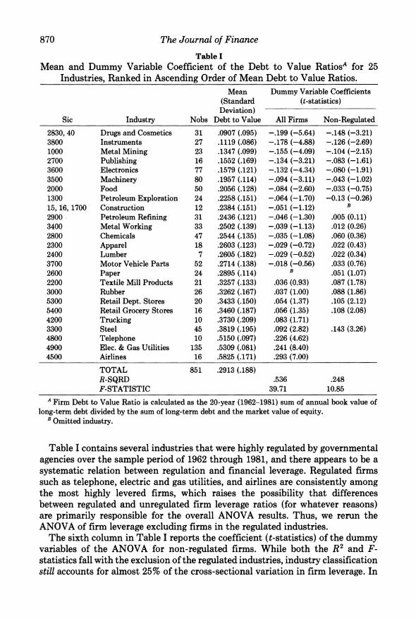
Summary Statistics, Correlation Matrix and Analysis of Variance on Industrial Classification of Firm VolatilityA, Non-Debt Tax

ShieldsB and Advertising and Research and Development Expenses'.

Non-Debt Tax Advertising and Volatility Shields R & D

Correlation Coefficients Volatility 0.05 -0.05 Non-Debt Tax Shields -0.25

Anova Results R-SQRD .337 .357 .562 F-Statistic 16.91 18.47 43.75

Summary Statistics Mean .053 .263 .020 Standard Deviation .038 .113 .030 Minimum .008 .020 .000 Maximum .332 .914 .221 A Firm Volatility is calculated as the standard deviation of the first difference in

annual earnings before interest, depreciation and taxes over the period 1962-1981 divided by the average value of total assets over the same time period.

B The level of firm Non-Debt Tax Shields is calculated as the ratio of the 20-year (1962-1981) sum of annual depreciation plus investment tax credits divided by the sum of annual earnings before interest, depreciation and taxes over the same period.

c The level of firm Advertising plus Research and Development expenses is given by the 10-year (1971-1982) sum of annual advertising, plus research and development expenses divided by the sum of annual net sales over the same period.

the agency costs of discretionary assets or their role as a non-debt tax shield, we expect the intensity of advertising and R&D expenses to be inversely related to firm leverage ratios. Our empirical measure of this variable is the sum of annual advertising and R&D expenses divided by the sum of annual net sales.11

Table II reports summary statistics of our three empirical proxies of the determinants of corporate leverage. The first two rows of the table report the correlation coefficients between each pair of these variables. The second two rows report the results of an analysis of variance of each variable on industrial classification, again using the dummy variable technique. The bottom four rows report summary statistics.

The R2 and F-statistics reported in Table II show that industry classifications are important determinants of our empirical proxies. Approximately 34% of the cross-sectional variation in firm volatility; 36% of non-debt tax shields, and 56% of advertising and R&D expenditures can be explained by industry variables. Therefore, each variable is a legitimate candidate for explaining the within industry similarities of firm leverage ratios documented in Table I.

" Due to limitations of the COMPUSTAT files regarding the reporting of these data, these sums are calculated only over the last 10-year interval of our sample period (1972-1981).

Theory and Evidence 873

Table III

Ordinary Least Squares Regression Results of Firm Debt to Value RatioA on Firm VolatilityB, Non-Debt Tax ShieldsC and Advertising plus Research and

Development ExpensesD, with and without Industry Dummy Variables for All and Non-Regulated Firms. All Firms Non-Regulated Firms

Firms 821 655

Industries 25 21

With Industry With Industry Without Industry Dummy Vari- Without Industry Dummy Vari- Dummy Variables ables Dummy Variables ables

Constant .330 .225 .202 .191 (19.96) (7.30) (11.24) (4.77)

Firm Volatility -1.73 -0.645 -0.806 -0.579 (-12.33) (-4.66) (-5.85) (-3.94)

Non-Debt Tax .370 .308 .423 .316 Shields (7.61) (6.51) (8.51) (6.12)

Advertising and -2.42 -0.98 -1.34 -0.956 R & D Ex- (-13.13) (-4.43) (-7.53) (-4.13) pense

R-SQRD .342 .586 .236 .337 F-Statistic 141.78 41.63 67.11 13.92

A Firm Debt to Value Ratio is calculated as 20-year (1962-1981) sum of annual book value of long- term debt divided by the sum of long-term debt and the market value of equity.

B Firm Volatility is calculated as the standard deviation of the first difference in annual earnings before interest, depreciation and taxes over the period 1962-1981 divided by the average value of total assets over the same time period.

c The level of firm Non-Debt Tax Shields is calculated as the ratio. of the 20-year (1962-1981) sum of annual depreciation plus investment tax credits divided by the sum of annual earnings before interest, depreciation and taxes over the same period.

D The level of firm Advertising plus Research and Development expenses is given by the 10-year (1971-1982) sum of annual advertising, plus research and development expenses divided by the sum of annual net sales over the same period.

C. Cross-Sectional Tests and Results

Table III reports the results of the cross-sectional regressions of firm leverage ratios on their hypothesized determinants. The table is divided into two major sections. The left hand side shows the regressions over all 821 firms in the sample.12 The right hand side shows the regressions over the 655 unregulated firms, which excludes firms in the trucking, telephone, electric and gas utility, and airline industries.

The data reported in the first column of Table III indicate that our measure of firm volatility is significant and negatively related to firm leverage ratios

12 The difference between this number and the 851 in Table I is due to missing data on the COMPUSTAT file.

874 The Journal of Finance

across the 821 firms in the sample. The t-statistic is -12.33. The data also show that the level of advertising and R&D expense is related negatively to firm leverage (t = - 13.13). These results are consistent with the implications of our theoretical model.

In contrast to firm volatility and to advertising and R&D expenditures, the sign of the coefficient on non-debt tax shields is perverse. The model predicts that non-debt tax shields, being substitutes for the tax benefits from debt financing, should be related inversely to firm leverage. The significant positive relation between leverage and the level of non-tax shields (t = 7.61) is in contradiction to this prediction.13

The lack of negative relation between non-debt tax shields and leverage ratios raises doubts as to the validity of DeAngelo and Masulis' argument that non- debt tax shields are substitutes for interest tax shields. The results suggest that firms that invest heavily in tangible assets, and thus generate relatively high levels of depreciation and tax credits, tend to have higher financial leverage. This is consistent with Scott's [25] "secured debt" hypothesis, which states that, ceteris paribus, firms can borrow at lower interest rates if their debt is secured with tangible assets.14

To examine the extent to which the independent variables reflect industry factors, we add a matrix of industry dummy variables to the regression model and re-estimate the coefficients on firm volatility, non-debt tax shields, and advertising and R&D expenses. The results of this expanded regression over all firms are reported in the second column of Table III. While the addition of the industry dummy variables reduces the magnitude and significance of the coeffi- cients of the independent variables, firm leverage ratios remain inversely related to firm volatility and to advertising and R&D expenses, and directly related to the level of non-debt tax shields.

The second half of Table III reports the results of our cross-sectional analysis of non-regulated firms. These data show that the results based on the full sample are not driven by a regulatory effect. Even across just the non-regulated firms, leverage is related negatively to firm volatility and to advertising and R&D expenses, and it is related positively to the level of non-debt tax shields. These results hold up when industry dummy variables are included in the regression.15

As a final test of the relation between firm leverage and our independent

13 The negative relation between leverage and advertising and R&D expenditures and the positive relation between leverage and non-debt tax shields are also reported by Titman [26].

14 This explanation implies that our cross-sectional regression is misspecified, because it omits an important independent variable, a proxy for secured debt. The positive correlation between the missing variable and the included variable measuring non-debt tax shield is the suspected reason for the seemingly perverse positive relation. This also raises the possibility that correlation between missing variable and the other included variables is causing us to misinterpret their coefficients as well.

15 Chaplinsky [2] also finds a negative relation between leverage and firm volatility; however, her t-statistics are substantially less than those reported in Table III. This difference may be due to the fact that her measure of leverage is based on the book value of total assets whereas our measure incorporates the market value of equity. As mentioned earlier, a measure of leverage based on the book value of equity is not consistent with the specification of the theory and hence is likely to produce weaker results.

Theory and Evidence 875

Table IV

Ordinary Least Squares Regression Results of Firm Debt to Value RatioA on Firm and Industry Measures of Volatility', Non-Debt Tax ShieldsC and

Advertising plus Research and Development ExpensesD for All and for Non- Regulated Firms.

All Firms Non-Regulated Firms

Firms 821 655

Industries 25 21

Without Industry With Industry Without Industry With Industry Means Means Means Means

Constant .330 .432 .202 .124 (19.96) (16.80) (11.24) (2.32)

Volatility -1.73 -0.658 -0.806 -0.583 (-12.33) (-4.23) (-5.85) (-3.83)

Non-Debt Tax .370 .312 .423 .317 Shields (7.61) (5.86) (8.51) (5.93)

Advertising and -2.42 -0.989 -1.34 -0.971 R & D Ex- (-13.13) (-3.99) (-7.53) (-4.06) pense

Industry Means:

Volatility -3.11 -0.843 (-11.59) (-2.46)

Non-Debt Tax .126 .526 Shields (1.30) (3.44)

Advertising and -2.36 -0.189 R & D Ex- (-6.74) (-0.42) pense

R-SQRD .342 .464 .236 .270 F-Statistic 141.78 117.41 67.11 39.84

A Firm Debt to Value Ratio is calculated as 20-year (1962-1981) sum of annual book value of long- term debt divided by the sum of long-term debt and the market value of equity.

B Firm Volatility is calculated as the standard deviation of the first difference in annual earnings before interest, depreciation and taxes over the period 1962-1981 divided by the average value of total assets over the same time period.

c The level of firm Non-Debt Tax Shields is calculated as the ratio of the 20-year (1962-1981) sum of annual depreciation plus investment tax credits divided by the sum of annual earnings before interest, depreciation and taxes over the same period.

D The level of firm Advertising plus Research and Development expenses is given by the 10-year (1971-1982) sum of annual advertising, plus research and development expenses divided by the sum of annual net sales over the same period.

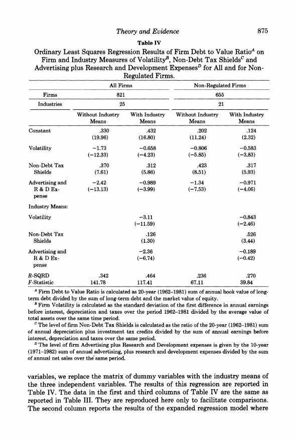
variables, we replace the matrix of dummy variables with the industry means of the three independent variables. The results of this regression are reported in Table IV. The data in the first and third columns of Table IV are the same as reported in Table III. They are reproduced here only to facilitate comparisons. The second column reports the results of the expanded regression model where

876 The Journal of Finance

industry mean values of firm volatility, non-debt tax shields, and advertising and R&D expenses are entered as independent variables.

The significance of the coefficients of the industry mean variables (reported in the lower half of the table) indicates that these industry means are at least partially responsible for the industry effects accounted for previously with the industry dummy variables. The R2 statistic falls from 59% (Table III) to 46% with this substitution. The lower R2 indicates that there are industry factors in addition to industry means of firm volatility, non-debt tax shields, and advertising and R&D expenses that can account for some residual cross-sectional variations in firm leverage ratios. Note also that, while including the industry means reduces the magnitude and significance of our firm-specific variables, the latter are still significantly different from zero.

The rest of Table IV repeats the regression over the subsample of non-regulated firms. Each of the firm-specific variables bears the same relation to firm leverage as it does in the overall sample. Moreover, the addition of the industry means does not materially affect either the magnitude or the significance of any of the firm-specific variables. The industry mean of advertising and R&D expenses, however, is not significant in this regression. This suggests that the industry mean of advertising and R&D expenses is proxying for regulation in the overall regression."

IV. Summary and Conclusions

This paper develops a model that synthesizes the modern balancing theory of optimal capital structure. This model incorporates positive personal taxes on equity and on bond income, expected costs of financial distress (bankruptcy costs and agency costs), and positive non-debt tax shields. We show that optimal firm leverage is related inversely to expected costs of financial distress and to the (exogenously set) amount of non-debt tax shields. A simulation analysis dem- onstrates that if costs of financial distress are significant, optimal firm leverage is related inversely to the variability of firm earnings.

The empirical section investigates the cross-sectional behavior of 20-year average firm leverage ratios for 851 firms covering 25 two-digit SIC industries. Several important results emerge. First, there exists strong industry influences across these firm leverage ratios. The cross-sectional regressions on industry dummy variables explain 54% of variation in firm leverage ratios. Excluding from the regression all regulated firms during the sample period, such as trucking, telephone, electric and gas utilities, and airlines, still yields an R2 of 25%.

Our search for the specific economic sources of these strong industry influ- ences on firm leverage ratios yields some noteworthy results. The volatility of firm earnings is an important, inverse determinant of firm leverage. It helps explain both inter- and intra-industry variations in firm leverage ratios. The intensity of R&D and advertising expenditures is also related inversely to leverage. Both of these results are consistent with the formal balancing model of optimal leverage.

16 Regulated firms have inordinately low advertising and R&D expenses.

Theory and Evidence 877

A somewhat puzzling finding is the strong direct relation between firm leverage and the relative amount of non-debt tax shields. This contradicts the theory that focuses on the substitutability between non-debt and debt tax shields. A possible explanation is that non-debt tax shields are an instrumental variable for the securability of the firm's assets, with more securable assets leading to higher leverage ratios.

A fundamental problem with the cross-sectional regressions is misspecifi- cation, which suggests a "missing variable" explanation for the perverse result on non-debt tax shields. The danger is that excluded variables are correlated with included variables, which can cause misleading inferences to be drawn from the regression results. Nonetheless, the strong finding of intra-industry similar- ities in firm leverage ratios and of persistent inter-industry differences, together with the highly significant inverse relation between firm leverage and earnings volatility, tends to support the modern balancing theory of optimal capital structure.

REFERENCES

1. Buser, S. and P. Hess, "The Marginal Cost of Leverage, the Tax Rate on Equity and the Relation between Taxable and Tax-Exempt Yields," Ohio State University Working Paper (October 1983).

2. Chaplinsky, S., "The Economic Determinants of Leverage: Theories and Evidence," Unpublished Ph.D. Dissertation, University of Chicago (September 1983).

3. Castanias, R., "Bankruptcy Risk and Optimal Capital Structure," Journal of Finance (December 1983).

4. Castanias, R. and H. DeAngelo, "Business Risk and Optimal Capital Structure," Unpublished Working Paper, University of Washington (1981).

5. DeAngelo, H. and R. Masulis, "Optimal Capital Structure Under Corporate and Personal Taxation," Journal of Financial Economics (March 1980).

6. Ferri, M. and W. Jones, "Determinants of Financial Structure: A New Methodological Approach," Journal of Finance (June 1979).

7. Flath, D. and C. Knoeber, "Taxes, Failure Costs, and Optimal Industry Capital Structure: An Empirical Test," Journal of Finance (March 1980).

8. Hamada, R., "The Effect of the Firm's Capital Structure on the Systematic Risk of Common Stocks," Journal of Finance (May 1972).

9. Harris, J., R. Roenfeldt, and P. Cooley, "Evidence of Financial Leverage Clienteles," Journal of Finance (September 1983).

10. Jensen, M. C. and W. H. Meckling, "Theory of the Firm Managerial Behavior, Agency Costs and Ownership Structure," Journal of Financial Economics (October 1976).

11. Kim, E. H., "A Mean-Variance Theory of Optimal Capital Structure and Corporate Debt Capacity," Journal of Finance (March 1978).

12. Kim, E. H., "Miller's Equilibrium, Shareholder Leverage Clienteles, and Optimal Capital Struc- ture," Journal of Finance (May 1982).

13. Kim, E. H., W. G. Lewellen, and J. J. McConnell, "Financial Leverage Clienteles: Theory and Evidence," Journal of Financial Economics (March 1979).

14. Kraus, A. and R. Litzenberger, "A State-Preference Model of Optimal Financial Leverage," Journal of Finance (September 1973).

15. Marsh, P. "The Choice between Equity and Debt: An Empirical Study," Journal of Finance (March 1982).

16. Miller, M. H. "Debt and Taxes," Journal of Finance (May 1977). 17. Modigliani, F., "Debt, Dividend Policy, Taxes, Inflation, and Market Valuation," Journal of

Finance (May 1982).

878 The Journal of Finance

18. Modigliani, F. F. and M. H. Miller, "The Cost of Capital, Corporation Finance, and the Theory of Investment," American Economic Review (June 1958).

19. Modigliani, F. F. and M. H. Miller, "Corporation Income Taxes and the Cost of Capital: A Correction," American Economic Review (June 1963).

20. Myers, S. C., "Determinants of Corporate Borrowing," Journal of Financial Economics (November 1977).

21. Remmers, L., A. Stonehill, R. Wright, and T. Beckhuiser, "Industry and Size as Debt Ratio Determinants in Manufacturing Internationally," Financial Management (Summer 1974).

22. Schwartz, E. and R. Aronson, "Some Surrogate Evidence in Support of the Concept of Optimal Financial Structure," Journal of Finance (March 1967).

23. Scott, D. F., "Evidence on the Importance of Financial Structure," Financial Management, (Summer 1972).

24. Scott, J., "A Theory of Optimal Capital Structure," Bell Journal of Economics (Spring 1976). 25. Scott, J., "Bankruptcy, Secured Debt, and Optimal Capital Structure," Journal of Finance (March

1977). 26. Titman, S., "Determinants of Capital Structure: An Empirical Analysis," Unpublished Working

Paper, UCLA (1983). 27. Titman, S., "The Effect of Capital Structure on a Firm's Liquidation Decision," Journal of

Financial Economics (forthcoming) 28. Trzcinka, C., "The Pricing of Tax-Exempt Bond and the Miller Hypothesis," Journal of Finance

(September 1982). 29. Trzcinka, C. and S. Kamma, "Marginal Taxes, Municipal Bond Risk and the Miller Equilibrium:

New Evidence and Some Predictive Tests," Unpublished Working Paper, State University of New York at Buffalo (December 1983).

DISCUSSION

WAYNE H. MIKKELSON*: The Bradley, Jarrell and Kim paper presents a single- period model of corporate capital structure for a firm with two classes of securities. Based on comparative statics and simulations of the model, three determinants of optimal capital structure are identified and empirically investigated in a cross- sectional examination of leverage ratios. The three determinants are: (1) costs of financial distress, (2) level of non-debt tax shields and (3) variability of firm value.

A linear ordinary least squares regression model is estimated to test empirical propositions drawn from the model and simulations. For a sample of 821 firms and using data drawn from the COMPUSTAT file, the ratio of the mean book value of long-term debt to the mean sum of market value of equity and book value of long-term debt for 1962-1981 is regressed on (1) the standard deviation of first differences in annual earnings divided by average value of total assets for 1962-81, (2) annual depreciation plus investment tax credits divided by annual earnings before interest, depreciation and taxes for 1962-81, and (3) annual advertising plus research and development expenses divided by annual net sales for 1971-1982. Regardless of whether the regression includes dummy variables for industry category, the coefficient on standard deviation of first differences in annual earnings is negative, the coefficient on the sum of depreciation and investment tax credits is positive and the coefficient on advertising and research

* University of Chicago and Dartmouth College (on leave). I would like to thank Larry Dann for his helpful comments.