American Institute of Aeronautics and Astronautics
1
Genetic Exchange Mechanisms for Co-Evolution In Decomposition-Based Design
J. Ryoo* and P. Hajela**
Mechanical, Aerospace and Nuclear Engineering Rensselaer Polytechnic Institute, Troy, NY 12180
Abstract
The paper examines new strategies for the implementation of genetic algorithms in a decomposition-based approach for design. In this approach, the design problem is decomposed into smaller-sized sub problems, the solutions for which are obtained through co-evolution. The emphasis resides in evaluating methods for exchanging design information relevant to coordinating solutions of temporarily decoupled sub problems. Methods based on modification of genetic makeup through experiential inheritance (exposure to another specie), and through inter species migration are investigated in this work. Different forms of design problem coupling are investigated, ranging from coupling through constraints only, to coupled objective and constraint functions. The proposed strategies are validated through implementation in representative algebraic and structural design problems.
Introduction Decomposition-based design methods
have been proposed as a solution to large-scale coupled problems, wherein the original problem is decomposed into a number of smaller, more tractable sub problems [1]. The ability to create smaller sub problems which represent the full complexity of the original problem, may allow for parallel processing of solutions and contribute to a better understanding of the problem domain. Traditional decomposition strategies fall into
three principal categories - object decomposition, aspect decomposition, and sequential decomposition. Object decomposition partitions a system into physical elements of the system, aspect decomposition seeks to decompose the problem based on the physics of the system, and sequential decomposition partitions the problem in a manner best suited to the flow of design information. The structure of typical design problems after decomposition may either be hierarchical or non-hierarchical, depending upon the coupling between the decomposed sub problems. The coupling may be hierarchical, where it is possible to identify distinct tree-like patterns of interaction or, no obvious hierarchy may exist, and there may be multiple one or two-way couplings among sub problems.
In order that the optimal solution to the original design problem is obtained through solutions of several smaller sized sub problems, solution coordination is necessary to account for any interactions among the decomposed sub problems. When using traditional gradient-based optimization methods, such interactions are typically considered on the basis of sensitivity information. Many problems, specifically those involving discrete and integer design variables are not amenable to such an approach due to the lack of gradient information; other problems may suffer from the existence of multiple relative optima and require that global search algorithms be used instead. The genetic algorithm has emerged as a leading global search method that increases the probability of identifying the global optimum in such generically difficult optimization problems.
In using GA’s in a decomposition based design environment [2,3], each sub problem is assigned a subset of design variables and those constraints, which are most critically
AIAA 2002-1674
*Graduate Assistant, **Professor, Fellow AIAA Copyright 2002 by P. Hajela . Published by the American Institute of Aeronautics and Astronautics, Inc. with permission
43rd AIAA/ASME/ASCE/AHS/ASC Structures, Structural Dynamics, and Materials Con22-25 April 2002, Denver, Colorado
American Institute of Aeronautics and Astronautics
2
affected by the variables. The genetic algorithm without any specialized treatment can handle these smaller sized sub problems. Once the sub problems are generated, GA based searches are conducted in parallel in each of the sub problems (co-evolution). However, the interactions between the temporarily decoupled sub problems must be appropriately considered, and in the absence of gradient information, constitute the principal challenge. The paper explores strategies by which changes in a sub problem are communicated to other sub problems. Modification of designs of a particular sub problem through exposure to designs in other sub problems, and inter-species migration of designs (from one sub problem to another), are considered in this work. It should be noted that such an approach allows for parallel processing of multiple populations, adding to the computational efficiency of the genetic search process. Subsequent sections of the paper describe typical forms of coupling that may be encountered in multidisciplinary design problems and solution strategies that were examined as candidates for these problems. Results obtained through the decomposition-based approach are compared with known analytical solutions and those obtained through an all-in-one (non-decomposition based) approach. Communication Based on Experiential Inheritance
The following mathematical representation describes a coupled design problem where the design variable vector X={XS,XA,XB} contains three subsets of variables; subsets XA and XB contain design variables encountered only in sub problems A and B, respectively.
=
= ≤
= ≤
( , , )
. ( , ) 0
( , ) 0
minimize f f X X XS A B
s.t g g X XA A S A
g g X XB B S B
(1)
The subset XS represents shared variables common to both of these sub problems; gA
and gB are sets of inequality constraints belonging to each of the sub problems, respectively. If the objective function is separable, in other words, if there is no coupling between XA and XB, the
optimization problem can be decomposed into two sub problems as follows.
=
= ≤
=
= ≤
( , )
( , ) 0
( , )
. ( , ) 0
minimize f f X XA A S A
s.t. g g X XA A S A
minimize f f X XB B S B
s.t g g X XB B S B
(2)
These two sub problems cannot be solved independently as a unique value for XS is required. There is a need, therefore, for coordination between the solutions of the two sub problems.
The experiential inheritance approach is based on a very crude model of cultural contact. An individual lives within a certain cultural group, responding to the inputs from the local environment. Some individuals of a group may have the occasion to encounter an individual from another cultural group. These contacts may enable individuals from both groups to identify significant differences; this learning experience is brought back into their native environment. Such a concept may be thought of as a modification in fitness values in the context of a genetic algorithm based search strategy. The fitness of an individual design can be evaluated in terms of the objective and constraint functions for a particular sub problem. This individual design may be compared to another from a different sub problem, and this exposure used to modify the fitness of the former. Then during genetic evolution in a particular sub problem, the modified fitness is used in lieu of the fitness indicated by the sub problems’ objective and constraint function values. The general procedure can be outlined as consisting of the following steps. Step 1. Generate populations randomly for each sub problem. Step 2. Evaluate the fitness values of each member of the population with respect to the objective and constraint functions of that sub problem. Step 3. Select two individuals for contact from the two sub problems, and compare their shared design variables.
American Institute of Aeronautics and Astronautics
3
Step 4. According to the individuals’ predefined comparison measure, modify the original fitness values of both. Steps 3 and 4 must be repeated for all members of the sub problem population. Step 5. Perform ordinary genetic algorithm operations with modified fitness values and repeat from Step 2 until a certain termination criterion has been satisfied.
Three distinct issues are pertinent in this approach. These include the selection of the two individuals for comparison, the metric for comparing these individuals, and the algorithm to modify their original fitness values.
First, either random or deterministic methods may be used for contact selection. In this paper, binary tournament selection from the previous generation was used for this purpose. Following the completion of Steps 3 and 4, the modified designs and their associated modified fitness values were said to comprise an experiential inheritance population. For the selection defined in Step 3, for every individual (I) in one population, two individuals were selected from the experiential inheritance population of another sub problem. Binary tournament selection was performed between the two individuals to choose the best (J) of the two. I and J were denoted as contact mates and a comparison was performed between these two; fitness of individual I was modified as indicated in eqn (4). This was repeated for each individual in all sub problems. Note that for the first generation, selection had to be performed randomly as modified fitness values had not been obtained as yet.
The comparison of two designs may be performed in various ways. In this work, difference of real values was used for comparison of shared design variables. One difference measure may be defined as follows,
α= −∑= 1
nDM x x
i Ai Bii
(3)
where, xi indicates shared design variables, n is the number of shared design variables, xA indicates that the value is from current sub problem A and xB indicates that the
value is from experiential inheritance population of sub problem B. Constant coefficient α is a weighting factor. For example, if x1 varies from 0.0001 to 0.0002 while x2 varies from 2 to 3, simple addition of differences may de-emphasize the difference in x1. Proper coefficient values ofα ’s would balance the significance of x1
and x2. Although not directly inspired from collaborative optimization method [4], it is interesting to note that this comparison method is somewhat analogous.
Following a comparison of individuals, the fitness values must be modified. In this study, the difference between two designs (DM) was appended as a penalty to the objective function; in a function minimization problem, decreasing the penalty would ensure greater compatibility between the two sub problems. The modified objective function is as follows,
objective DMγ= +modified objective (4)
where the coefficient γ should be increased as DM decreases to improve the matching continually. Note that the objective term as defined in Eqn. (4) may include any penalty term associated with the violation of the design constraints.
For purposes of selection, the modified objective values in each sub problem were converted to areas on a roulette wheel as follows,
_
worst objectivearea
worst ave objective−=
−(5)
where worst is the maximum modified objective value, and ave_objective is the population average of the current modified objective values. Communication Between Sub Problems Using Interspecies Migration
The optimization problem of Eqn. (1) cannot be decomposed into sub problems as described in Eqn (2) when there is cross coupling between components of XA and XB
in the objective function. However, such a problem can be decomposed into two sub problems as follows.
American Institute of Aeronautics and Astronautics
4
=
≤
=
≤
*( , , )
*( , , )
minimize f f X X XA S A B
s.t g = g (X , X ) 0 A A S A
minimize f f X X XB S A B
s.t g = g (X , X ) 0B B S B
(6)
Here, the variables with asterisk are referred to as migration variables, and are not included in the chromosomal representation of the design for a particular sub problem. Therefore, these variables do not participate in the crossover and mutation operations. However, these variables are needed to compute objective values. For example, without the value of XB*, fA cannot be computed in sub problem A; the value of XB*is obtained from sub problem B.
Various options are available for this choice of XB*. The XB value of the best design in sub problem B may be used; alternatively, XB can be chosen at random from all designs in sub problem B. In this study, a tournament selection method was used to select values of migration variables. From an experiential inheritance population under consideration, a certain number of designs were selected, the best out of the selected designs was chosen, and the migration variables of the chosen design were used for objective function calculation. It is important to bear in mind that the objective values of the experiential population have been modified as in eqn. (4 ). For each individual design in a sub problem, the value of the migration variable was obtained through a separate selection process; the values of migration variables in a given population can, therefore, be different for each individual.
Note that the tournament size determines the performance of the strategy. A tournament size of 1 defines a random selection from the population whereas a tournament size equal to the size of the population implies selecting the best design. In this study, binary tournament was used. Communication of System Response Using Interspecies Migration
There is a class of coupled problems where the coupling is not through design variables directly, but rather, through
response or behavior variables. The general mathematical statement of this class of problems may be written as follows,
, X )B
with
s.t.
=
=
=
= ≤
= ≤
( ,
( , , )
( , , )
( , , ) 0
( , , ) 0
minimize f f X XS A
Y Y X X YA A S A B
Y Y X X YB B S B A
g g X X YA A S A A
g g X X YB B S B B
(7)
where YA and YB are sub problem responses. They represent the coupling if sub problems A and B are to be considered separately. The constraints of these sub problems require YA and YB, and these in turn are dependent on each other. It is interesting to note that optimization of these problems without decomposition is not an easy task. If the response equations are linear in terms of Y’s, the solution is relatively easy. However, if they are nonlinear, solving such a system of equations can prove to be a challenge. If a response relation is not expressed in terms of mathematical equations, such as data correlation, response surface, or neural network mapping, the feasibility of obtaining Y’s directly from X’s is questionable. An optimization problem with system responses can be decomposed as follows if there is no coupling between XA and XB.
with
with
=
∗=
= ≤
=
∗=
= ≤
( , )
( , , )
. . ( , , ) 0
( , )
( , , )
. . ( , , ) 0
minimize f f X XA A S A
Y Y X X YA A S A B
s t g g X X YA A S A A
minimize f f X XB B S B
Y Y X X YB B S B A
s t g g X X YB B S B B
(8)
Here Y*’s represent migration responses much like the migration variables in the previous section; these cannot be obtained directly within a particular sub problem. As in the previous section, a binary tournament selection was used to select values of migration response variables. Elitist Communication and Consistency of Selection
Following the GA evolution of the local population in each sub problem, the best
American Institute of Aeronautics and Astronautics
5
performer was identified. These individuals were then matched against each other for experiential inheritance and migration communication. This elitist selection was used in lieu of the tournament selection described earlier.
In this study, only one tournament selection was performed for experiential inheritance and communication of interspecies migration. Therefore, the shared design variable values for comparison, the migration design variables for objective function, and the system responses are from one individual in an experiential inheritance population. In this way, combination of favorable factors from various designs is avoided, which may generate incompatible designs.
In some cases, the only coupling may be through shared variables in the objective and constraint functions. However, it is sometimes beneficial to include information (through migration communication) of objective and constraint function terms that depend on variables that are typically not active in a given sub problem, as this can help the performance of the search process. The test problems examined in this paper include examples of such problem formulations. A stepwise description of the process used in this study is outlined below and a schematic illustration of the process for a two-sub problem case is shown in Figure 1. Step 1. Generate populations randomly for each sub problem. Step 2. For each individual in sub problem populations, find a contact mate by performing binary tournament selection from experiential inheritance populations (of another sub problem) defined in Step 5; the tournament selection is based on the modified objective value. The preserved elitist individuals in Step 6 are specifically matched against each other instead of using tournament selection. For the first generation of co-evolution, perform random selection. Step 3. Evaluate the objective values of each population (note that the objective
includes an appended measure of constraint violation). When the evaluation needs a migration design variable value and/or response value, use the values associated with the contact mate identified as described in Step 2. Step 4. Use the experiential inheritance approach to obtain modified objective values. Step 5. Associate design variables and system responses with the modified objective value computed in Step 4 to form experiential inheritance populations. These experiential inheritance populations are used in step 2 where contact mates are identified. Step 6. Perform ordinary genetic algorithm operations with modified fitness values and go to Step 2. Repeat until a prescribed termination criterion has been satisfied.
Random population
Evaluation
Modify Objective value
Experiential Inheritance Population
GA operations
Random population
Evaluation
Modify Objective value
Experiential Inheritance Population
GA operations
Migration communication
Experiential Inheritance
Figure 1 Illustration of Co-Evolution
Numerical Examples
The proposed strategies have been implemented in several algebraic problems and a stiffened composite panel design problem. These test problems are described next. Problem 1: The first problem is representative of a case where the objective function is separable; a shared variable xo
represents the coupling in the design constraints.
American Institute of Aeronautics and Astronautics
6
= + +
= + ≤
= + ≤
2 2 20 1 2
. 1 - 01 0 1
1- 02 0 2
minimize f x x x
s.t g x x
g x x
(9)
The problem can be decomposed into two sub problems as follows. Sub Problem 1-A
= + +
= = + ≤
= ≤
2 2 *21 0 1 2
. 1 - 01 1 0 1
* 02 2
minimize f x x x
s.t g y x x
g y
(10)
Sub Problem 1-B
= + +
= = + ≤
= ≤
2 *2 22 0 1 2
1- 03 2 0 2
* 04 1
minimize f x x x
s.t. g y x x
g y
(11)
This problem was solved using the experiential inheritance approach to provide solution coordination among the sub problems; results of ten different simulations are presented in Table 1. The decomposition does not specifically require
that the term *22x and *2
1x be included in the objective functions of sub problem 1-A and 1-B, respectively. Similarly, the constraints
*2y and *
1y are not required in the sub problems. The inclusion of these terms, obtained from the experiential inheritance population of the previous generation, contributes to improved solution efficiency.
Problem 2: The first problem was extended to assess the performance with larger number of variables. A test problem with 24 design variables was formulated as follows.
242
1
8 16
11 9
8 24
21 17
8 0
8 0
ii
i ii i
i ii i
f x
g x x
g x x
=
= =
= =
=
= + − ≤
= − + ≤
∑
∑ ∑
∑ ∑
minimize
s.t. (12)
This problem was decomposed in a manner similar to that used for the first problem; results obtained in the test runs are presented in Table 2.
Problem 3: A problem with non-linear
objective function was formulated as follows.
21 3
1 1 2
2 1 3
2cos
2 1 0
0
xf x e x
g x x
g x x
π= + += − + ≤= − + ≤
minimize
s.t. (13)
The decomposition for this problem was as follows. Sub Problem 3-A
2 *1 1 3
1 1 1 2
*2 2
2cos
2 1 0
0
xf x e x
g y x x
g y
π= + += = − + ≤
= ≤
minimize
s.t. (14)
Sub Problem 3-B
*2
2 1 3
3 2 1 3
*4 1
2cos
0
0
xf x e x
g y x x
g y
π= + += = − + ≤
= ≤
minimize
s.t. (15)
Problem 4: To test the applicability of the
proposed scheme in problems with greater number of sub problems, the following problem was formulated.
= + +
= + ≤
= + ≤
= + ≤
2 2 21 2 3
. 1- 2 01 1 2
1- 2 02 2 3
1- 2 03 3 1
minimize f x x x
s.t g x x
g x x
g x x
(16)
The problem decomposition strategy resulted in 3 sub problems as follows. Sub Problem 4-A
= + +
= = + ≤
= ≤
= ≤
2 *2 *21 1 2 3
1- 2 01 1 1 2
* 02 2
* 03 3
minimize f x x x
s.t. g y x x
g y
g y
(17)
Sub Problem 4-B
= + +
= = + ≤
= ≤
= ≤
*2 2 *22 1 2 3
1- 2 04 2 2 3
* 05 1
* 06 3
minimize f x x x
s.t. g y x x
g y
g y
(18)
American Institute of Aeronautics and Astronautics
7
Sub Problem 4-C
= + +
= = + ≤
= ≤
= ≤
*2 *2 23 1 2 3
. 1- 2 07 3 3 1
* 08 1
* 09 2
minimize f x x x
s.t g y x x
g y
g y
(19)
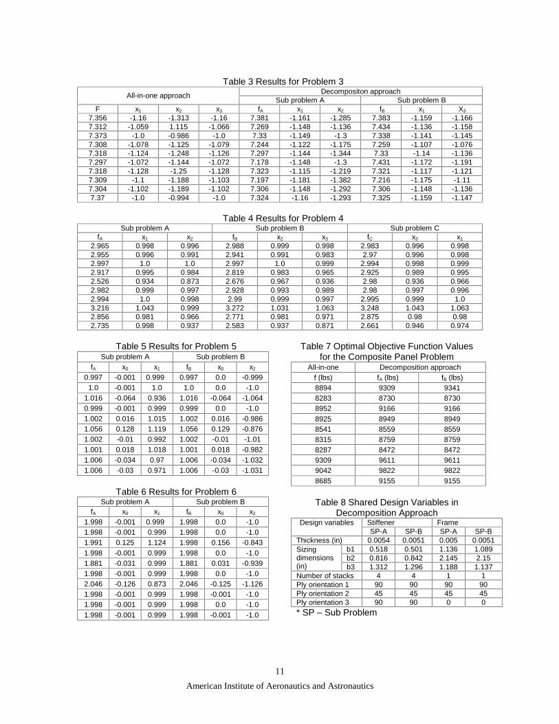
Results for this test problem are summarized in Table 4.
Problem 5: The introduction of cross coupling in design variables was introduced by the addition of a coupled term in the first test problem as follows.
= + + +
= + ≤
= + ≤
2 2 20 1 2 1 2
. 1 - 01 0 1
1- 02 0 2
minimize f x x x x x
s.t g x x
g x x
(20)
The decomposed problem used the migration strategy to get x2 for objective function in sub problem 5-A and x1 for sub problem 5-B. The topology for decomposition was as follows. Sub Problem 5-A
= + + +
= = + ≤
= ≤
2 2 *2 *1 0 1 2 1 2
1 - 01 1 0 1
* 02 1
minimize f x x x x x
s.t. g y x x
g y
(21)
Sub Problem 5-B
= + + +
= = + ≤
= ≤
2 *2 2 *2 0 1 2 1 2
1- 03 2 0 2
* 04 1
minimize f x x x x x
s.t. g y x x
g y
(22)
A summary of test results for this problem is presented in Table 5.
Problem 6: To study the decomposition-based approach in problems where an additional coupling is introduced through response variables computed in different sub problems, the following test problem was established.
= + +
= + +
= +
= ≤
= ≤
2 2 20 1 2
1 -1 0 1 2
1- -2 0 2 1
01 1
02 2
minimize f x x x
with y x x y
y x x y
s.t. g y
g y
(23)
The decomposed problem used a migration strategy to carry information of y1 from sub problem 6-A to sub problem 6-B and vice versa for y2. A mathematical statement of the two decomposed problems is as follows. Sub Problem 6-A
= + +
= + +
= ≤
= ≤
2 2 *21 0 1 2
*1 -1 0 1 2
01 1
* 02 2
minimize f x x x
with y x x y
s.t. g y
g y
(24)
Sub Problem 6-B
= + +
= +
= ≤
= ≤
2 *2 22 0 1 2
*1- -2 0 2 1
. 03 2
* 04 1
minimize f x x x
with y x x y
s.t g y
g y
(25)
Note that for this problem, compatibility is required not only for design variables but also for system responses. To facilitate such compatibility, special steps may be required. As an example, consider a case where an individual of sub problem 6-A with x0 = 0.5 and x1 = 0.5 is compared against an individual of sub problem 6-B with x0 = 0.5, x2 = -0.5, and y2 = -1.0. In such a comparison, compatibility of shared design variable x0 would be satisfied as would the corresponding local constraints. However, for designs in sub problem 6-B to evolve to these values (x0 = 0.5, x2 = -0.5, and y2 = -1.0) during a similar comparison against another member of sub problem 6-A, incoming y1 from that individual of sub problem 6-A would have to be 1.0. This may be possible when the population is diverse, as is the case in earlier stages of the evolution process. However, as variables converge within a sub problem, these
American Institute of Aeronautics and Astronautics
8
compatibility requirements would be progressively more difficult to satisfy. To address this problem, the size of tournament selection pool was progressively decreased. For example, in the first generation of evolution, tournament was held between two individuals randomly selected from a whole population. After a fixed number of generations, the tournament was restricted to two individuals randomly selected from a predefined set of best designs. This process was continued, with a steadily shrinking set of best designs from which candidates for the tournament were selected; a minimum pool size of 5 was found to be effective in this approach. Results for this numerical problem are presented in Table 6.
In all of these algebraic problems, the design variables x were restricted to the range –2.0 to 2.0. A total of 100000 function evaluations were permitted and a population of size 100 was used for each sub problems for all simulations where each evaluation in each sub problem accounts for one function evaluation.
Figure 2 Skin-stringer panel
Problem 7. The seventh example problem deals with coordinating two weight minimizing sub problems. Each sub problem contains both sizing variables and those describing the layup of the composite stiffened panels shown in Figure 2. Two panels are adjacent each other under independent boundary conditions and loads while sharing the design of their stiffeners and frames.
The number of C-frames determines the number of bays in the structure, and consequently, the number of different composite layups to be obtained. Therefore, the left panel with 2 frames has a single bay with one composite layup to be obtained and the right panel has 3 frames and 2 bays, each with a different layup. While the design of bays was considered to be independent for each panel, the stiffener and frame designs were considered to be common to both sub problems. The design variables for stiffeners and frame were therefore considered as shared design variables in this problem.
Figure 3 Composite laminate layup
The frames, stiffeners, and the composite skin were a graphite/epoxy laminate with a layup sequence as shown in Figure 3. The 5 variables used to represent the composite layup were the number of stacks, composite orientations of each of the 3 plies in a stack, and the thickness of a ply. The ply orientations could be chosen from 4 discrete possibilities (45, -45, 0, and 90 deg). The layup could consist of 1, 2, 4 or 6 stacks. In a given layup, the ply thicknesses were identical. Each frame and stiffener had sizing variables as shown in Figure 4. When calculating the difference measure, scaling of variable values was required to balance their individual contributions to the measure. For discrete design variables such as number of stacks and ply orientations, simple checking of equality was applied. For example, if two compared designs had the same number of stacks, nothing was added to the difference measure. However, if they have different number of stacks and were therefore incompatible, the difference measure was incremented by ∆DM=1.
American Institute of Aeronautics and Astronautics
9
Figure 4 C-beam design variables The panel was analyzed using a finite
element approach for a number of random variations in design variables taken over the design domain. A back-propagation neural network was used to construct a surrogate model for analysis, mapping the design variables into constraints such as panel bucking eigenvalue, local panel buckling, stringer crippling failure, and Johnson-Euler buckling in the stringers.
Results and Discussions
To account for the random nature of the
search process, multiple simulations were conducted for each problem, using different random number seeds in each case. Table 1 shows the results obtained for algebraic function described in Problem 1.
Analytical solution to this problem is x0 = 0,
x1 = 1.0, and x2 = -1.0 with f = 2.0. For most of the cases, the search process was able to reach the true solution with small incompatibilities. For example, the second case has two different x0 values (–0.001 and 0.0). Stressing the experiential inheritance penalty more heavily may eliminate this incompatibility. However, improperly weighted penalty terms may degrade the search process; this is also highly problem dependent. In the present example, the coefficients of penalty terms associated with local constraints started at a value of 2.0, and were increased by 1.0 every 10 GA generations when less than 50% of designs were feasible; the coefficients for experiential inheritance started with 2.0 and were increased by 1.0 every 10 GA generations.
Similar sets of results were obtained for problem 2 and are summarized in Table 2. Table 2 shows objective value in both sub problems and the solution compatibility and constraint violations. Satisfied constraints
are shown as 0 in the Table. Optimal solution has an objective value of 16.0. This problem had eight shared variables. So, the first run case in sub problem A shows a compatibility violation (CV) 0.04, indicating that on average there is 0.005 difference in shared design variables of sub problem A and B.
Table 3 shows the results of all-in-one searches and decomposed searches of a non-linear algebraic problem. The search results are comparable in both search algorithms and the compatibility violations in x1 are maintained at acceptably small levels.
Problem 4 is representative of a fully
coupled problem. Sub problem A is coupled with sub problem B through x2 and also to sub problem C though x1. Likewise, sub problem B involves sub problems A and C, and sub problem C involves sub problems A and B. The optimal solution of the problem has an optimal objective function of 3.0 with each design variable at 1.0. A summary of numerical results for 10 different GA simulations is presented in Table 4 in order of quality of the solution.
The results from numerical experiments
performed for Problem 5 are summarized in Table 5. This problem is not only coupled through constraints but also through objective function. It has an optimal objective of 1.0 with x0=0, x1=1, and x2=-1.
Test problem 6 has response coupling in
its constraints. Therefore, in a decomposition based design environment, use of migration communication is essential in solving the problem. The optimal objective of 2.0 is obtained for x0=0, x1=1, and x2=-1.
Results for the weight minimization of the stiffened composite panel are summarized in Table 7; comparison of results for the all-in-one approach and decomposition approach (10 different simulations) are presented in this table. The minimal weight was identified in the all-in-one search as 8287 lbs; this compares favorably against the design of 8472 lbs identified in the decomposition based approach. Although the average performance of search process was slightly better in all-in-one approach, there was considerable variation in the
American Institute of Aeronautics and Astronautics
10
results in both strategies suggesting maintaining greater diversity in the search process and significantly higher number of function evaluations in both cases. The effectiveness of the coordination method in the decomposition approach is illustrated by the compatibility in the shared variables. For the test case corresponding to an optimal weight of 8472 lbs, a comparison of shared variables is presented in Table 8. These variables include dimensions and composite layup sequences for stiffeners and frames. As seen in the table, the differences in the design variables are relatively small.
Closing Remarks
The paper examines new strategies for
adapting a GA search in a decomposition based design environment. In this approach, communication between the decomposed sub problems is most critical to direct the search towards a globally compatible solution. The paper proposes an approach referred to as experiential inheritance, wherein individuals from different sub problems are compared on the basis of numerical values of their shared variables, and the differences used in determination of their survival. A communication strategy, referred to as migration, is proposed to complete any response information within a sub problem that is not being computed in that sub problem. It is worthwhile to note that entire populations within the sub problems participate in information communication; communication is not based on a single representative design within a sub problem. The paper presents results from numerical experiments conducted for various forms of problem coupling, and the results show that the proposed strategies are effective in obtaining solutions comparable to those obtained in the all-in-one approach. The decomposition-based approach should lend itself better to a parallel processing environment.
Acknowledgements Research support for this work under a
grant from the Sikorsky Aircraft Company is gratefully acknowledged.
References
[1] Sobieszczanski-Sobieski, J. And Haftka, R. T., “ Multidisciplinary Aerospace Design Optimization: Survey of Recent Developments,” Structural Optimization, Vol. 14, pp. 1-23, 1997. [2] Lee, J., and Hajela, P., "Parallel Genetic Algorithm Implementation in Multidisciplinary Rotor Blade Design", AIAA Journal of Aircraft, Vol. 33, No. 5, pp. 962-969, 1996. [3] Lee, J., and Hajela, P., "GA’s in Decomposition Based Design - Subsystem Interactions Through Immune Network Simulation", Structural Optimization, vol. 14, No. 4, pp. 248-255, December 1997. [4] Kroo, I., et. al.,”Multidisciplinary optimization methods for aircraft preliminary design,” AIAA Paper No. 94-4325, 1994.
Table 1 Results for Problem 1 Sub problem A Sub problem B