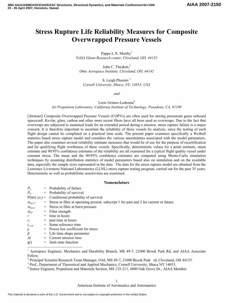
American Institute of Aeronautics and Astronautics

1

Stress Rupture Life Reliability Measures for Composite

Overwrapped Pressure Vessels

Pappu L.N. Murthy

1

NASA Glenn Research center, Cleveland, OH, 44135

John C. Thesken,2

Ohio Aerospace Institute, Cleveland, OH, 44142

S. Leigh Phoenix 3

Cornell University, Ithaca, NY, 14853, USA

and

Lorie Grimes-Ledesma4

Jet Propulsion Laboratory, California Institute of Technology, Pasadena, CA, 91109

[Abstract] Composite Overwrapped Pressure Vessels (COPVs) are often used for storing pressurant gases onboard

spacecraft. Kevlar, glass, carbon and other more recent fibers have all been used as overwraps. Due to the fact that

overwraps are subjected to sustained loads for an extended period during a mission, stress rupture failure is a major

concern. It is therefore important to ascertain the reliability of these vessels by analysis, since the testing of each

flight design cannot be completed on a practical time scale. The present paper examines specifically a Weibull

statistics based stress rupture model and considers the various uncertainties associated with the model parameters.

The paper also examines several reliability estimate measures that would be of use for the purpose of recertification

and for qualifying flight worthiness of these vessels. Specifically, deterministic values for a point estimate, mean

estimate and 90/95% confidence estimates of the reliability are all examined for a typical flight quality vessel under

constant stress. The mean and the 90/95% confidence estimates are computed using Monte-Carlo simulation

techniques by assuming distribution statistics of model parameters based also on simulation and on the available

data, especially the sample sizes represented in the data. The data for the stress rupture model are obtained from the

Lawrence Livermore National Laboratories (LLNL) stress rupture testing program, carried out for the past 35 years.

Deterministic as well as probabilistic sensitivities are examined.

Nomenclature

Pf, = Probability of failure

PS = Probability of survival

P(t|σ(.),t1) = Conditional probability of survival

σop1,2 = Stress in fiber at operating present. subscript 1 for past and 2 for current or future.

σburst = Stress in fiber at burst pressure

σtef = Fiber strength

t = time in hours

t1 = past time in hours

tc,ref = Some reference time

ρ = Power law coefficient for stress

β = Life time shape parameter

∆t = Current mission time

g() = limit state function

1 Aerospace Engineer, Mechanics and Durability Branch, MS 49-7, 21000 Brook Park Rd, and AIAA Associate

Fellow. 2 Principal Scientist Research Team Manager, OAI, MS 49-7, 21000 Brook Park rd, Cleveland, OH 44135. 3 Prof., Department of Theoretical and Applied Mechanics, Cornell University, Ithaca NY 14853. 4 Senior Engineer, Propulsion and Materials Section, MS 125-211, 4800 Oak Grove Dr., AIAA Member

48th AIAA/ASME/ASCE/AHS/ASC Structures, Structural Dynamics, and Materials Conference<br> 15th23 - 26 April 2007, Honolulu, Hawaii

AIAA 2007-2150

This material is declared a work of the U.S. Government and is not subject to copyright protection in the United States.

American Institute of Aeronautics and Astronautics

2

fX = Joint probability density function

Xv = Vector of random variables X1, X2,…. Xn

I. Introduction

S with any pressure vessel, risk of failure must be mitigated through an understanding of the failure modes.

In particular, metallic pressure vessels are typically designed to exhibit the failure mode called “leak-before-

burst”. The concept is that leakage results from slow stable crack growth from an initial small flaw, causing a slow,

noticeable leak of the contents. This serves as advance warning to retire the vessel before a disastrous burst occurs,

releasing stored energy that would likely cause loss of life and significant, possibly catastrophic damage to the

spacecraft. COPVs are susceptible to most of the same failure modes as metallic pressure vessels, since the metallic

liners have the same mechanical properties, but additional considerations arise from the use of the composite

overwrap.

While the metallic liner of a COPV can also exhibit the leak-before-burst failure mode, the composite overwrap

is susceptible to other failure modes that are not predictable using such fracture mechanics based prediction tools.

Because the composite in a COPV carries a large portion of the pressure load during operation, failure modes

associated with the failure of the composite must be considered during the design and operation of these COPVs. In

the case of COPVs, there are two primary but related failure modes that can appear after successful qualification of a

COPV design: these are stress rupture and loss of structural integrity due to impact damage, which may cause

immediate burst failure or may contribute to the stress rupture process. Both of these failure modes can result in the

sudden, catastrophic failure of the pressure vessel without the advance warning that is possible with all-metal

pressure vessels. A COPV that fails due to the stress rupture failure mode will burst suddenly and with no warning

leading to catastrophic consequences such as loss of a vehicle and the crew.

Stress rupture life testing for Kevlar has been performed primarily by Lawrence Livermore National

Laboratories (LLNL) and Cornell University with additional Kevlar material characterization contributions from the

Y12 Plant at Oak Ridge National Laboratory and Sandia National Laboratories. These tests have consisted of

single-fiber, fiber-bundle, resin impregnated strand (or tow tests), and small COPVs testing at several fixed stress

levels1-4.

Although models based on data from LLNL, Cornell, and DOE are available in the literature, they are neither

directly comparable nor applicable to any other COPV designs that are used on spacecraft. Changes have to be

made to account for the load carrying effects of the liner, the effects of strength variations between different spools

used to overwrap the COPVs, volume fraction effects of the matrix and compensation for differences in ultimate

burst strength of the composite due to differences in pressurization rate between the spacecraft COPVs and the small

COPVs tested by LLNL. In addition, corrections to account for Kevlar creep relaxation need to be made.

During the last three years there have been two independent technical assessment activities for reassessing the

safety of Kevlar and Carbon fiber COPVs on board spacecraft; sponsored by the NASA Engineering Safety Center

(NESC)1-2. The work reported here pertains to stress rupture life reliability models discussed in detail in the

aforementioned references.

II. Stress Rupture Life Reliability: Phoenix Model

It is customary to utilize a Weibull statistics based approach to fit stress rupture life data, and this was done with

the original LLNL test data. There are a number of models that exist with some variations, and this is discussed in a

separate paper5. For the current discussion the Phoenix model is used. The Phoenix model has been developed over

the past 27 years and is well documented in the literature6-7. It is based on a Weibull distribution framework for

strength and lifetime with the embodiment of a power law to describe damage in a composite versus stress level.

Derivation of the model is available in references where the power-law in stress level (with temperature

dependence) is derived from thermally activated chain scission using a Morse potential as a model8. The model

A

American Institute of Aeronautics and Astronautics

3

parameters are based on the LLNL epoxy-impregnated strand and pressure vessel data. In the simplest setting of

constant stress applied quickly and maintained over a long time period, the basic equation for the model is below:

−−=

βρ

σ

σσ

burst

op

refct

ttP

,exp1),( (1)

where P(t, σ) represents the probability of failure at time t subjected to applied stress σ. In the above equation the quantity (σop / σburst) is the ratio of the nominal fiber stress at operating pressure to the nominal fiber stress at burst

pressure (called the fiber stress ratio), t is time, tc,ref is a reference time, ρ is the power law exponent, and β is the

Weibull shape parameter for lifetime. The fiber stress ratio may be established either by using simple netting

analysis in combination with thin shell mechanics or via a detailed finite element analysis. The complete details

pertaining to stress ratio calculations as well as the above equation are available in ref. 1. The value for σburst is

determined from the flight COPV burst test data accounting for pressurization rate differences between flight

COPVs and the COPVs tested by LLNL1. The model is shown for a fixed fiber stress level over time, but for more

general time histories a memory integral is used to accumulate damage (similar to Miner’s rule for fatigue) at

varying stress levels. Also, at very high fiber stress levels a second quantity within square brackets and of similar

structure to the first must also be included with a leading minus sign as well (i.e., in a weakest damage mechanism

framework). This second quantity has different parameter values, especially a much higher ρ value, and applies to

times on the order of 100 hours or less, whereas the parameter values we consider apply to much longer times.

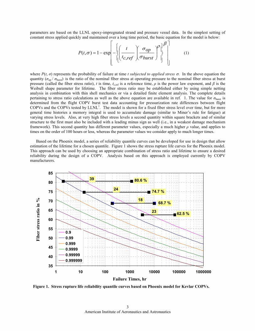
Based on the Phoenix model, a series of reliability quantile curves can be developed for use in design that allow

estimation of the lifetime for a chosen quantile. Figure 1 shows the stress rupture life curves for the Phoenix model.

This approach can be used by choosing an appropriate combination of stress ratio and lifetime to ensure a desired

reliability during the design of a COPV. Analysis based on this approach is employed currently by COPV

manufacturers.

35

40

45

50

55

60

65

70

75

80

85

1 10 100 1000 10000 100000 1000000

Failure Times, hr

Fib

er str

ess ra

tio in %

0.9

0.99

0.999

0.9999

0.99999

0.999999

80.6 %

74.7 %

68.7 %

62.5 %

39

24

18

23

Figure 1. Stress rupture life reliability quantile curves based on Phoenix model for Kevlar COPVs.

American Institute of Aeronautics and Astronautics

4

Also indicated in Fig. 1 are data from the original LLNL experiments on small Kevlar COPVs for stress rupture

life. The four horizontal lines indicate the failure times in hours of vessels that failed in stress rupture at different

stress ratio levels. The number of vessels that failed in stress rupture at each of these stress ratios is 39, 24, 18 and

23 out of about 25 to 50 vessels that were held at each stress ratio. The actual data points indicating times to failure

in hours is not shown in the above chart. Only the range of values is indicated by the horizontal lines at different

stress ratio levels. Further details can be found in ref. 1. No failures were noted at the lowest stress ratio, 0.446 by

the time the experiments were stopped and the program had ended. Substantial scatter exists in stress rupture failure

lifetimes (almost three orders of magnitude) as seen in the figure.

III. Conditional Probability of Survival

For recertification purposes of COPVs that have been under successful operation for a prolonged time, however,

a conditional probability approach needs to be used (in essence ruling out unusually short lived vessels within the

population since none actually occurred). In this approach, at any reference time all successful history prior to this

instant is considered in the analysis and credit is taken of this successful past history in the computation of future

probability of survival. The conditional failure probability equation for the Phoenix model given in Eq. 1, can be

easily derived with the application of Bayes Theorem9 as shown below:

( )

+

∆+

−−=⋅

βρβρρ

σ

σ

σ

σ

σ

σσ

ref

op

refcref

op

refcref

op

refc t

t

t

t

t

tttP

1

,

12

,

1

,

11 exp1),(

(2)

Where P(t|σ(.),t1) represents the probability of failure at time t, given survival with stress history σ(.) to time t1. In this equation, two new terms appear, one for a second, new, stress level and another to account for past history at

a previous stress level. The second stress level is introduced to account for any procedural or operational changes to

be made for the future missions (such as lowering operational pressure) in order to improve reliability estimates.

As an illustration of the above equation a sample problem is chosen where the reliability is computed for two

different operating stress ratios (S.R) 0.575 and 0.45. The past survival history amounts to 3743 hours and current

mission time is 100 hours. The parameter ρ is taken as 24, β is taken as 1.2 and tc,ref is taken as 0.5457 hours. With a

ratio of 0.575, the calculated reliability is 0.9998 while it is 0.9999999 when a ratio of 0.45 is used. If we had been

operating the vessel at 0.575 during the entire history of 3743 hours and decided to reduce the ratio to 0.45 for future

missions in order to improve the survival probability the result is 0.9999996. An interesting observation is that it is

the future mission hours at a specified stress ratio that is most important in determining the survival probability. Past

history has only a minimal effect in this formulation.

The sensitivity of the conditional probability of survival to various stress rupture life parameters of interest is shown

in Figure 2. Each variable is normalized with respect to the point value (nominal values chosen for the parameters)

and is varied one at a time from 0.4 to 1.4. In the example the nominal values chosen are S.R = 0.575, ρ = 24, β =

1.2, and tc,ref = 0.5457. From Fig. 2, it is clear that the conditional survival probability is most sensitive to variables

stress ratio and the power law coefficient ρ, while it is fairly insensitive to the values of tc,ref and β.

American Institute of Aeronautics and Astronautics

5

Figure 2. Sensitivity of the conditional probability of survival to various normalized stress rupture life

estimation parameters. In the legend shown S.R represents Stress Ratio, Beta represents β, Rho represents ρ and T

Ref represents tc,ref.

IV. Probability of Survival for a System of COPVs

Stress rupture failure of a COPV has a catastrophic implication of loss of vehicle and crew. The importance, of

accurate reliability estimation for each COPV as well as the system of COPVs as a unit cannot be overemphasized.

In addition, while computing the reliabilities, one must consider that there are a number of vessels on board a typical

spacecraft at various pressures and age and therefore one has to account for all this to arrive at a system level

probability of survival which implies survival of every vessel for this duration of mission. In the following section

typical calculations are shown for a system of 24 vessels grouped into 5 different sub-systems. Survival of the entire

system of vessels in a mission is crucial to successful mission.

Computation of System Level Survival Probability

For the collective system of vessels the chance for failure of any one of the vessels is derived using the “rare event

probability approximation” by the following:

1

1 n

i

f S

i

P P=

= −∑ (3)

where Pf is the chance of any one of the vessels failing due to stress rupture during a mission and PS is the

probability of survival of a specific vessel. The above equation is sufficiently accurate for Pf << 1(rare event

probability approximation). The probability of survival PS for a system of vessels is given by

fP1SP −= (4)

The probabilities of failure and survival for individual vessels as well as the system of vessels as a unit are computed

for a 24 vessel COPV system and details are shown in Table 1.

0.999

0.9991

0.9992

0.9993

0.9994

0.9995

0.9996

0.9997

0.9998

0.9999

1

0.4 0.6 0.8 1 1.2 1.4

Normalized Parameters

Probability of Survival

S.R.

Beta

Rho

T Ref

S

American Institute of Aeronautics and Astronautics

6

Table 1. Typical Spacecraft COPV Sub-Systems and Reliability Estimations

COPV

Sub-

System

Past

Accumulated

Time t1

(Hours)

Current

Estimated

Mission

Time

(Hours)

No of

vessels

Past OP

Stress

Ratio

Proposed

Mission

Stress

Ratio

Conditional

Probability

of Survival

Conditional

Mission

Probability

of Failure

A-1 3743 100 1 0.575 0.575 0.99984546 0.0001545

A-2 3431 100 1 0.575 0.575 0.99984809 0.0001519

B 1-2 6254 195 2 0.515 0.515 0.99998602 0.0000280

B 3-4 5875 195 2 0.515 0.515 0.99998619 0.0000276

B 5-6 5686 195 2 0.515 0.515 0.99998628 0.0000274

C-1 834 24 3 0.54 0.54 0.9999955 0.0000135

D-2 834 24 7 0.47 0.47 0.99999992 0.0000006

E-1 73847 648 1 0.445 0.445 0.99999887 0.0000011

E-2 73847 648 1 0.445 0.445 0.99999887 0.0000011

E-3 73760 648 1 0.445 0.445 0.99999887 0.0000011

E-4 65262 648 1 0.445 0.445 0.9999989 0.0000011

E-5 61145 648 1 0.445 0.445 0.99999891 0.0000011

E-6 21900 648 1 0.445 0.445 0.99999911 0.0000009

System Probability of Survival 24 0.99958998 0.0004100

Typical Spacecraft COPV Sub-Systems: Reliability Estimations

Vessel subsystems A, B, C, D and E perform various functions, such as Orbit maneuvering, main propulsion,

environmental control and life support, and are generally filled with inert gasses such as Nitrogen and Helium. The

details are extremely specific to the type of space craft. In the computations it is assumed that the same operating

stress ratios are in effect for the past successful history as well as the future/current missions (σop1=σop2). As

mentioned earlier, if computed reliability is below a desired threshold then the current mission operating conditions

need to be adjusted so that a lower stress ratio is achieved.

V. Parameter Uncertainties

In general when dealing with reliability one must assess and account for two types of uncertainties epistemic

uncertainty and aleatory uncertainty. Epistemic uncertainty arises due to lack of knowledge, or insufficient data.

Such uncertainties can be reduced over time with more experiments and experience. On the other hand aleatory

uncertainty is the so called physical variability that is present in almost all the systems and is unlikely to be

reducible. Various publications address these two types of uncertainty and the importance of separating and

resolving them11-12

.

These uncertainties are especially critical for the COPVs because of the risks and costs involved. Model form or

epistemic uncertainty can be reduced by collecting more data and by developing better analytical relationships. Here

we attempt to show how the model-form uncertainties affect the reliability estimates via Monte Carlo simulations of

the conditional probability of survival.

The conditional probability of survival given by Equation (2) is a function of several variables and parameters

which have been determined based on limited amounts of data. Furthermore the scatter in failure times as noted in

the LLNL data often encompasses two to three orders of magnitude. Uncertainties in the model parameters therefore

will have substantial effects on the computed reliabilities. Consequently, deterministic treatment of various

parameters in arriving at a single point probability of survival estimate can not be stated with high confidence so that

one must consider the confidence bounds on these estimates. Accordingly the point probability estimate becomes a

random variable and hence one needs to bound this with either upper or lower confidence bounds or one sided

confidence bounds to account for uncertainty in parameter estimates. An attempt is made to capture these with the

Phoenix model and is presented in this section.

Equation (5) is an expression for probability of survival in a generic form as a function of several pertinent

random variables representing uncertainties

American Institute of Aeronautics and Astronautics

7

),,rt,rt,r(F)t,(SP βρ∆σ=σ (5)

where

ref,c

1r σ

σ=σ , (6)

ref,ct

1trt = , (7)

ref,ct

1trt

∆=∆ (8)

The symbols ρ and β are the stress power law exponent and the shape factor respectively. A limit state function

(sometimes referred to as performance function) is defined as:

0SP)X(SP)X(g −= (9)

Where PS0 is a particular value of PS. The vector X represents the various uncertain variables considered in the

current problem, and these will have a joint uncertainty distribution Xf as we now describe. The limit state function

can be an implicit or explicit function of random variables and is divided in such a way that ( ) 0=Xg is a

boundary between the region [g ≤ 0], which means that a certain level of reliability is not met, and [g > 0], which

means the reliability is exceeded. It should be noted that since the cumulative distribution function (CDF) of PS at

PS0 equals the probability that [g ≤ 0]. The CDF can be computed by varying PS0 and computing the point

probability each time.

The probability that [g ≤ 0], is then given by the integral

1 2 1 2( , ,.... ) ..[ 0] ...

X n nX X X dX dX dXP g fΩ

≤ = ∫ ∫ (10)

in which fX(X1, X2 , …, Xn) is the joint probability density function for variables X1, X2 … Xn and the integration is

performed over the region, Ω, where g ≤ 0. If the random variables are statistically independent, then the joint

probability density function can be replaced by individual density functions. This integral can be computed by

standard Monte Carlo procedure which is rather straightforward. However, depending upon the number of random

variables involved and the level of PS0 sought, this must be repeated thousands of times, to accurately build the

response variable’s probabilistic characteristics. Although inherently simple, the large number of output sets that

must be generated to build the CDF of the output variable, becomes its obvious disadvantage. Furthermore, if the

deterministic computation of the response is complicated, requiring a time-consuming analysis (e.g. a large non-

linear finite element analysis), then the time required and the computational costs could become prohibitive. These

procedures are embedded in the NESSUS (Numerical Evaluation of Stochastic Structures under Stress) computer

code10, developed by Southwest Research Institute (SWRI).

VI. Point, Mean, and 95% Confidence Estimates for Kevlar Vessels

In the Phoenix model, values for the parameters tc,ref, ρ, and β are determined based on the LLNL vessel data and

are influenced by observations of stress rupture behavior of the strands and single fibers. Due to limited amount of

data, (especially, at lower stress ratios) all these parameters must be considered to have uncertainties with respective

uncertainty distributions associated with these parameters. One can compute reliability based upon nominal values

for these parameters (obtain using maximum likelihood methods applied directly to the lifetime data) and establish

the so called point estimate for the reliability. For a fixed set of parameter values the reliability is known exactly

through the model. However, such estimates always contain hidden dangers due to the fact that these parameters do

have uncertainties associated with them and therefore a probabilistic approach must be adopted to compute mean

values of the reliability integrating over the parameter uncertainty distributions. Similarly one can calculate lower

American Institute of Aeronautics and Astronautics

8

confidence bounds on the reliability estimate at some confidence level such as 90 or 95%. A typical uncertainty

distribution on failure probability, based upon 1000 Monte-Carlo simulations, is shown in Fig. 3. Here the values

for the parameters assumed are tc,ref = 0.5457, ρ = 24, and β = 1.97. The uncertainty distributions for these

parameters are taken as normal (Gaussian) for all the variables with coefficients of variation representative of the

LLNL data sample sizes

Figure 4 shows a normal probability plot of reliability where the x axis represents a transformed variable of

reliability to indicate basically the “number of nines” for each Monte-Carlo simulation. As shown in the figure the

mean probability of survival for this simulation is 0.999993 while the 95% confidence value is 0.9998. A point

estimate based on deterministic analysis indicates the probability of survival to be 0.999996. This is a common

situation whereby the mean is less than the point estimate. The cause is that the mean weighs the uncertainty with

respect to parameter values that though infrequent can dramatically increase the probability of failure. In other

words when an extremely low probability of failure is required and a high probability of failure can result for some

parameter combinations, then it is important that these combinations be extremely rare – not just fairly infrequent.

In fact, when data sets are small, it is possible for the mean to lie below, the 95% confidence value.

0

20

40

60

80

100

120

0.00

0000

1

0.00

0001

7

0.00

0003

7

0.00

0009

7

0.00

0015

7

0.00

0021

7

0.00

0027

7

0.00

0033

7

0.00

0039

7

0.00

0045

7

0.00

0051

7

0.00

0057

7

0.00

0063

7

0.00

0069

7

0.00

0075

7

0.00

0081

7

0.00

0087

7

0.00

0093

7

Probability of Failure

Frequency

0%

10%

20%

30%

40%

50%

60%

70%

80%

90%

100%

Frequency

Cumulative %

Figure 3. Probability of failure histogram constructed from 1000 Monte-Carlo simulations for

typical Composite Overwrapped Pressure Vessel using the Phoenix Model of conditional

probability of failure for Kevlar overwrap.

American Institute of Aeronautics and Astronautics

9

A. Determination of parameter uncertainties:

As mentioned before, the model parameters are established utilizing Weibull statistics and Maximum Likelihood

Estimates (MLE). However depending upon the available data at each stress level, the uncertainty in the parameters

vary and estimates for their distribution mean and standard deviation can be made via Monte Carlo simulation

techniques. To illustrate this parameter β is chosen and the details are described below.

90%95%

99%

PointMean

95%

90%95%

99%

PointMean

95%

Figure 4. Normal probability plot of Reliability expressed in terms of number of nines. Reliability in number of

nines = -log10 (Probability of failure).

American Institute of Aeronautics and Astronautics

10

Figure 5 shows a Monte Carlo simulation of the uncertainty distribution for an MLE of the Weibull shape

parameter β (actually 1 β ) given sample sizes from as low as 5 to as high as 320. Also shown in the plot are

numerical calculations based on the likelihood function for a sample size of 27, indicated by red line with circle

symbols. Note that when the sample size is only 10, an MLE estimate can easily be in error by 25 percent either

way. This is important because a serious overestimate of reliable lifetime can result simply due to natural variability

in samples of size 10, and this should be properly weighed against the probability it could occur. Larger sample

sizes, of course, greatly reduce the risk. Similarly the distribution statistics for all the parameters can be established

via computational simulation.

VII. Case Study: System Reliability Projections into Future Missions

The concepts discussed above can be utilized to project individual vessel as well as the system of all the vessels

on board reliabilities for future missions. As an example a case study is described here to illustrate how the various

metrics for reliability play an important role in determining the future flight reliability for the purpose of

recertification of successfully flown system of spacecraft COPVs. The details are provided in Table 2.

Table 2 shows various COPV subsytems present on board a typical spacecraft with their accumulated past time

in hours at a specific stress ratio (col. 2) and an estimated typical future mission time (col. 3) at the same stress ratio

(col. 5). The parameters for the model chosen with uncertainties associated with them are presented in Table 3.

For each COPV subsystem a separate Monte-Carlo simulation with 10,000 samples each is conducted with the

NESSUS10 software and relevant response statistics (mean, point and confidence bounds) are collected from the

output to fill in the various columns in Table 2. The point estimate for the COPV system survival is found to be

0.999987 while the mean, 95% and 90% estimates are 0.999949, 0.99976 and 0.99987, respectively. An interesting

point to note is that due to parameter uncertainty, the mean and various confidence bounds indicate significantly

lower reliabilities compared to the almost six nine reliability indicated by the point estimate.

Figure 5. Monte Carlo simulation results for parameter uncertainty statistics

American Institute of Aeronautics and Astronautics

11

Table 2. Typical Spacecraft COPV Sub-Systems and Reliability Estimations

COPV Sub-

System

Past

Accumulated

Time

(Hours)

Mission

Time

(Hours)

No of

vessels Stress Ratio

Mean Prob.

Survival

95%

Confidence

Prob.

Survival

90%

Confidence

Prob.

Survival

Point Prob.

Survival

A-1 4113 116 1 0.575 0.99998200 0.99991940 0.99995650 0.99999503

A-2 3801 116 1 0.575 0.99998300 0.99992130 0.99995770 0.99999526

B 1-2 6797 132 2 0.515 0.99999900 0.99999600 0.99999820 0.99999989

B 3-4 6418 132 2 0.515 0.99999900 0.99999610 0.99999820 0.99999989

B 5-6 5824 27 2 0.515 1.00000000 0.99999920 0.99999960 0.99999998

C-1 9212 140 3 0.54 0.99999600 0.99998110 0.99999030 0.99999913

D 1-3 9514 181 3 0.47 1.00000000 0.99999960 0.99999980 0.99999999

D 4-7 2006 70 4 0.47 1.00000000 0.99999990 0.99999990 1.00000000

E-1 75452 1468 1 0.445 1.00000000 0.99999880 0.99999950 0.99999998

E-2 75452 1468 1 0.445 1.00000000 0.99999880 0.99999950 0.99999998

E-3 75365 1468 1 0.445 1.00000000 0.99999880 0.99999950 0.99999998

E-4 66867 1468 1 0.445 1.00000000 0.99999880 0.99999950 0.99999998

E-5 62750 1468 1 0.445 1.00000000 0.99999890 0.99999950 0.99999998

E-6 23505 1468 1 0.445 1.00000000 0.99999910 0.99999960 0.99999999

System Probability of Survival 24 0.99994900 0.99975820 0.99987320 0.99998708

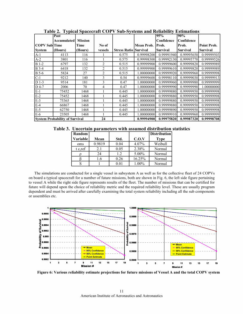
Table 3. Uncertain parameters with assumed distribution statistics

Random

Variable Mean Std. C.O.V

Distribution

Type

oms 0.9819 0.04 4.07% Weibull

t c,ref 2.1 0.05 2.38% Normal

ρ 24 1.2 5.00% Normal

β 1.6 0.26 16.25% Normal

S 1 0.01 1.00% Normal

The simulations are conducted for a single vessel in subsystem A as well as for the collective fleet of 24 COPVs

on board a typical spacecraft for a number of future missions, both are shown in Fig. 6, the left side figure pertaining

to vessel A while the right side figure represents results of the fleet. The number of missions that can be certified for

future will depend upon the choice of reliability metric and the required reliability level. These are usually program

dependent and must be arrived after carefully examining the total system reliability including all the sub components

or assemblies etc.

0.9940

0.9950

0.9960

0.9970

0.9980

0.9990

1.0000

1 3 5 7 9 11 13 15 17 19

Mission #

Probability of Survival

Mean

95% Confidence

90% Confidence

Point Estimate

0.9982

0.9984

0.9986

0.9988

0.999

0.9992

0.9994

0.9996

0.9998

1

1 3 5 7 9 11 13 15 17 19

Mission #

Probability of Survival

Mean

95% Confidence

90% Confidence

Point Estimate

0.9940

0.9950

0.9960

0.9970

0.9980

0.9990

1.0000

1 3 5 7 9 11 13 15 17 19

Mission #

Probability of Survival

Mean

95% Confidence

90% Confidence

Point Estimate

0.9982

0.9984

0.9986

0.9988

0.999

0.9992

0.9994

0.9996

0.9998

1

1 3 5 7 9 11 13 15 17 19

Mission #

Probability of Survival

Mean

95% Confidence

90% Confidence

Point Estimate

Figure 6: Various reliability estimate projections for future missions of Vessel A and the total COPV system

American Institute of Aeronautics and Astronautics

12

VIII. Conclusion

Stress rupture of composite overwraps can cause catastrophic consequences leading to loss of crew and

spacecraft and hence the reliability of these vessels during the entire duration of a space program must be carefully

examined and assessed. The present paper illustrates via a stress rupture life model proposed originally by Phoenix

how the probability of survival of individual as well as a system of vessels on board a typical space craft can be

computed systematically. Additionally, various reliability metrics such as point estimates, mean estimates, and

90/95/99% one sided confidence bounds are discussed. Epistemic or model-form uncertainties are assessed by using

Monte Carlo Simulation techniques. Such reliability estimates are essential in decision making and certification

processes regarding how long (or number of missions) a program should continue before the vessels are either

retired or subjected to another recertification process.

Acknowledgments

The authors wish to acknowledge the sponsorship provided by the NASA Engineering Safety Center for the

Kevlar and Carbon Independent Technical Assessment.

References 1Shuttle Kevlar Composite Overwrapped Pressure (COPV) for Flight Concern Technical Consultation Report, Vol. I and II,

NESC Publication, 2007 2Shelf Life Phenomenon and Stress Rupture Life of Carbon/Epoxy Composite Overwrapped Pressure Vessels (COPVs)

Technical Consultation Report, Vol. I and II, Dec. 2006. 3Glaser, R.E., R.L. Moore, and T.T. Chiao. “Life Estimation of an S-Glass/Epoxy Composite under Tensile Loading.”

Composites Technical Review, Vol. 5, No. 1 (1983): 21-26. 4Glaser, R.E., R.L. Moore, and T.T. Chiao. “Life Estimation of Aramid/Epoxy Composites under Sustained Tension.”

Composites Technical Review, Vol. 26 (1984): 26.

5Lorie Grimes-Ledesma and Pappu L.N. Murthy, “Comparisons of Stress-Rupture Models for COPV Life Prediction”. To be

presented at the 48th SDM conference, Hawaii, April 23-26, 2007. 6Phoenix, S. Leigh, and E.M. Wu. “Statistics for The Time Dependent Failure of Kevlar-49/Epoxy Composites:

Micromechanical Modeling and Data Interpretation.” IUTAM Symposium on Mechanics of Composite Materials, Pergamon

(1983):135. 7Phoenix, S. Leigh. “Statistical Modeling of the Time and Temperature Dependent Failure of Fibrous Composites.”

Proceedings of the 9th US National Congress of Applied Mechanics, Book # H00228, ASME, NY (1982): 219-229. 8Phoenix, S. Leigh, and Tierney, L. J. “A Statistical Model for the Time Dependent Failure of the Unidirectional Composite

Materials under Local Elastic Load-Sharing Among Fibers”, Engineering Fracture Mechanics, Vol. 18, No. 1, pp 193-215, 1983. 9Haldar, A. and Mahadevan, S. Probability, Reliability and Statistical Methods in Engineering Design, Wiley, New York

2000, pp. 25-28 10NESSUS (Numerical Evaluation of Stochastic Structures Under Stress). Final NASA Code, New manuals, version 6.2,

Southwest Research Institute, San Antonio, TX, 1995 11Helton J.C. and Burmaster, “Treatment of Aleatory and Epistemic Uncertainty in Performance Assessments for Complex

Systems”, Reliability Engineering and System Safety: Special Issue on Aleatory and Epistemic Uncertainties, 1996: 54 : 91-4. 12Hoffman F.O. and Hammonds, J.S., “Propagation of Uncertainty in Risk Assessments: The Need to Distinguish Between

Uncertainty Due to Lack of Knowledge and Uncertainty Due to Variability”, Reliability Engineering and System Safety, 1994:

14: 707-12.