American Institute of Aeronautics and Astronautics
1
Reliability Estimation of Large-Scale Structural Vibration Problems
Zissimos P. Mourelatos* Mechanical Engineering Department, Oakland University, Rochester, MI 48309-4478
Efstratios Nikolaidis† Mechanical, Industrial and Manufacturing Engineering Department, The University of Toledo, Toledo, OH 43606
Jared Song‡ Mechanical Engineering Department, Oakland University, Rochester, MI 48309-4478
Finite element (FE) analysis is a well-established methodology in structural dynamics. However, probabilistic studies can be prohibitively expensive because they require repeated FE analyses of large models. Various re-analysis methods have been proposed with the premise to effectively calculate the dynamic response of a structure after a baseline design has been modified, without recalculating the new response. Although they improve the computational efficiency considerably, they are not efficient enough for probabilistic analysis of large-scale vibration problems because they can only generate a relatively small number of sample points for a practically acceptable CPU time. In this paper, an efficient re-analysis method is used to generate a finite number of response sample points. Subsequently, tail modeling is used to estimate the right tail of the response PDF. This methodology enables us to accurately estimate high reliability values of vibratory problems with a relatively small number of analyses. A probabilistic vibration analysis of a realistic vehicle FE model is presented to demonstrate the advantages of the proposed probabilistic methodology.
I. Introduction Continuous efforts of the aerospace, automotive and shipbuilding industries to minimize the structural weight of
vehicles while maintaining an acceptable level of safety have compel engineers to develop reliable and efficient design optimization techniques. In many structural design situations the operating conditions, material properties and the geometry are uncertain. Optimizing the design in the face of uncertainty requires quantification and control of the risk of failure. For this purpose, these industries are trying to incorporate risk-based analysis and design in product development.
Probabilistic methods are being increasingly accepted by the industry [1-8]. These methods use probability theory and statistics to model uncertainty and to determine the probability of failure of a design. Then a designer can perform optimization to find the design with minimum weight, which satisfies the limits of the allowable probability of failure. A designer faces many challenges when applying reliability analysis and design to real-world problems. Finding the probability of failure of a given design requires repeating the structural analysis for different sets of the values of the random variables, which may be computationally expensive, especially when using finite element analysis [1-3]. Also, the computational expense may be grossly compounded when calculating the probability of failure of different designs during the search for an optimum reliability-based design.
Two methods are commonly used to calculate the reliability of a design; Monte-Carlo simulation techniques [1-3, 8-11] and analytical reliability approximate methods (e.g., the First Order Reliability Method, the Second Order Reliability Method and the Advanced Mean Value Method). The analytical reliability approximation methods find the Most Probable Point (MPP) for the design, which is an optimization problem [1-3, 12-15].
* Professor, member AIAA † Professor, member AIAA ‡ Research Associate
49th AIAA/ASME/ASCE/AHS/ASC Structures, Structural Dynamics, and Materials Conference <br> 16t7 - 10 April 2008, Schaumburg, IL
American Institute of Aeronautics and Astronautics
2
Attempts have been made to reduce the cost of reliability based analysis and design. For example, some researchers have developed efficient surrogate models (e.g., response surface polynomials and neural networks) to approximate the structural response and then used these approximate models to perform reliability-based design [16-21]. Others approximated the reliability function itself [22, 23]. Yet, these approximate models can be computationally very expensive to develop or may be highly inaccurate [24], especially when there are many random variables (e.g., more than 10).
Another way to reduce the computational effort of probabilistic analysis and design is by constructing physics-based approximations of the deterministic response. These approximations use basis functions obtained by analyzing representative designs, instead of generic basis functions, such as polynomials or exponential functions. Because of the superior quality of the basis functions, physics based approximations are accurate over a wide range of the random variables and still they are more efficient than structural analysis. This paper uses two physics-based approximations, parametric reduced basis models and a modified combined approximations method for probabilistic analysis of complex structures.
The main idea of the proposed paper is to calculate the upper tail of the response CDF of large-scale structural vibration problems accurately, without resorting to a large number of computationally demanding analyses. Note that the accurate estimation of the upper tail of the CDF ensures an accurate estimation of high reliability (small probability of failure). Because of the multi-modal behavior (multiple resonance peaks) of vibratory response, the failure domain usually consists of multiple disjoint “islands” which are scattered in the entire design domain. For this reason, the commonly used MPP-based analytical techniques (e.g. FORM, SORM) do not work for this class of problems. We will therefore, use ideas from simulation-based methods without using though, a very large number of sample points.
The proposed method consists of an efficient deterministic re-analysis and a PDF tail modeling approach. First we generate a limited number of sample points by performing a vibration analysis at selected points throughout the design domain. An efficient re-analysis method [25] is used which is substantially more efficient than the conventional modal (reduced-order) models. The sample points from the first step can theoretically be used to estimate the response PDF using methods such as the Polynomial Chaos Expansion (PCE) method [26] or the Maximum Likelihood Estimation (MLE) method [27], among others. The tail of the PDF will not be however, accurate because of the limited sample points. For this reason, the tail behavior of the response is obtained in this paper using a tail modeling approach [28-30] which utilizes the generalized Pareto distribution (GPD) to calculate the conditional excess distribution above a certain threshold.
The paper is organized as follows. In section 2, an overview of the re-analysis methodology is provided including an introduction to reduced order modeling for dynamic systems, and the Parametric Reduced Order Modeling (PROM), Combined Approximations (CA) and Modified Combined Approximations (MCA) methods [25]. Section 3 provides a brief overview of the fundamentals of tail modeling. The accuracy of the proposed probabilistic methodology for high reliability is demonstrated in section 4 using a hypothetical example and a complex vehicle model. The former demonstrates the merits of tail modeling.
II. Overview of Re-Analysis Method Finite element analysis (FEA) is a well-established numerical simulation method for structural dynamics. It
serves as the main computational tool for NVH analysis in the low-frequency range. However, the computational cost for large-scale models (more than one million degrees of freedom) can be excessive even for high-end workstations with the most advanced software. There are also other factors that increase the computational costs. When design changes are involved, the FEA analysis must be repeated many times in order to obtain the optimum design. Furthermore in probabilistic analysis where parameter uncertainties are present, the FEA analysis must be repeated for a large number of sample points. In such cases, the computational cost is even higher, if not prohibitive.
Re-analysis methods are intended to analyze efficiently structures that are modified due to various changes. The objective is to evaluate the structural response for such changes without solving the complete set of modified analysis equations. Several reviews have been published on re-analysis methods [31-33]. This section provides an overview of a new re-analysis method [25] which will be used in this study.
American Institute of Aeronautics and Astronautics
3
2.1 Reduced Order Modeling for Dynamic Response For an undamped structure with stiffness and mass matrices K , and M respectively, under the excitation force
vector F , the equations of motion (EOM) for frequency response are [ ] FdMK =− 2ω , (1)
where the displacement d is calculated at the forcing frequency ω . If the response is required at multiple frequencies, the repeated direct solution of Eq. (1) is computationally very expensive and therefore, impractical for large scale finite-element models.
The reduced order model (ROM) can be constructed using a subspace projection method. Instead of solving the original response equations, it is assumed that the solution can be approximated in a subspace spanned by the retained mode shapes. A modal response approach can be used to calculate the response more efficiently. A set of eigen-frequencies iω and corresponding eigenvectors (mode shapes) iφ are first obtained. Then, the displacement
d is approximated in the reduced space formed by the first n modes as ΦUd = , (2)
where [ ]nφφφΦ L21= is the modal basis and U is the vector of principal coordinates or modal degrees of freedom (DOF). Then the EOM of Eq. (1) can be transformed from the original physical to the modal degrees of freedom as
[ ] FΦUMΦΦKΦΦ TTT =− 2ω . (3) Solving for the modal response U and projecting it back to the physical coordinates, the response d can be
recovered. Due to the modal truncation, the size of the ROM is drastically reduced, compared to the original model. However, the size increases as the maximum excitation frequency increases.
2.2 Parametric Reduced-Order Modeling Method
The parametric reduced-order modeling (PROM) method is a subspace approximation method developed to improve the efficiency of re-analysis. It assumes that the dynamic response of a new design, which is obtained by relatively large parameter changes from the baseline design, can be approximated in the subspace spanned by the mode shapes of some representative designs.
The quality of the approximation depends on the selection of the representative designs. Originally Balmes et al. [34, 35] and subsequently Zhang et al. [36, 37] suggested a procedure for obtaining such designs. Consider a design defined in terms of m design parameters (for example plate thicknesses, spot weld diameters, spot weld pitch of a car body, etc.). The ranges in which these parameters and their baseline values can vary are estimated by the designer. In Zhang et al. [36, 37], the first representative design 0p is at the point with all design parameters at their lower limits. Additional m representative design points mii ,,1, L=p are obtained by perturbing the design parameters from their lower limits to their upper limits, one at a time. The points representing these designs in the space of the design parameters will be called corner points. Therefore, the total number of representative design points is ( )1+m .
In the PROM approach [36], the mode shapes of a new design, with stiffness and mass matrices pK and pM ,
are approximated in the subspace P spanned by the modes of the above ( )1+m designs,
[ ]mΦΦΦP K10= , (4) where 0Φ is the modal matrix composed of retained mode shapes for the baseline design, and iΦ is the modal
matrix for the thi design point, which is the same as the baseline design except that its thi parameter is at its upper limit.
For m design parameters, ( )1+m eigenvalue problems must be solved in order to form matrix P of Eq. (4). Therefore, both the cost of obtaining modal matrices iΦ and the size of matrix P increase linearly with the number of parameters. Basis P captures the dynamic characteristics in each dimension of the parameter space because it consists of mode shapes corresponding to the centers of the faces of a box representing the ranges of the parameters. The response at a new design point of the parameter space can be therefore, approximated accurately using basis P .
The following algorithm is used by the PROM approach to compute the mode shapes of a new design: 1) Find the modes of the baseline design and the designs corresponding to the m points in the design space, and
form subspace basis P .
American Institute of Aeronautics and Astronautics
4
2) Condense matrices pK and pM as
PMPMPKPK pT
RpT
R == , (5)
3) Perform an eigen-analysis on the reduced matrices RK and RM to calculate eigenvector Θ . 4) Reconstruct the approximate eigenvectors pΦ~ using
PΘΦ =p~
. (6) In the above procedure, step 1 is performed only once. For any repeated re-analysis, only steps 2 to 4 need to be
repeated. For a small number of modes and a few number of design parameters, the cost of steps 2 to 4 should be much smaller than the cost of a full analysis. Therefore, the PROM method could be a very efficient re-analysis method in such a case.
However the computational cost of steps 2 to 4 can become very high when the number of modes and/or the number of parameters m are large. The reason is that the cost of forming the condensed matrices (by computing the triple matrix products in Eq. (5)) can be high because subspace basis P is a large matrix with high density.
The computational cost of PROM consists of the costs involved in the following calculations: a) ( )1+m full
eigen-analyses to form subspace basis P in Eq. (4), and b) the cost of re-analysis of each new design. The cost involved in step a) is called fixed cost of PROM because it cannot be attributed to the calculation of the response of a particular design; it is required in order to obtain the information needed to apply PROM to a given problem. The cost of re-analysis of a new design (cost of b)) represents the variable cost and is trivial compared to the fixed cost, if the number of columns of P is low.
The following two observations can be made on the PROM approach. First, the fixed cost is proportional to the number of design parameters. Therefore, the efficiency of the PROM method is best demonstrated when the number of re-analyses is significantly larger than the number of design parameters. This is the case in simulation-based probabilistic analysis. Second, further improvement of the efficiency of the PROM approach requires reduction of the fixed cost.
A modified combined approximations (MCA) method and a Kriging interpolation method have been introduced and integrated with the PROM method to improve the efficiency of the PROM method by largely reducing its fixed cost. A brief description is provided below.
2.3 The Combined Approximations (CA) and the Modified Combined Approximations (MCA) Methods
The Combined Approximations (CA) method, which has been developed recently by Kirsch [38-40], combines the strengths of both local and global approximations, being accurate even for large design changes. The CA method is a combination of binomial series (local) approximations (also called Neumann expansion approximations) and reduced basis (global) approximations. Originally, the CA method was developed for linear static re-analysis. However, the method has been recently extended to eigen-problem re-analysis [41-45]. Accurate results and significant computational savings have been reported. A comparative study [46] has shown that the method is suitable for large design changes.
The PROM method requires calculation of the eigenvectors of multiple designs to form a basis for approximating the eigenvectors at other designs. In this study, a modified CA method (MCA) [25] which is an improvement of the original CA method [41-45], is used to circumvent the need to solve the eigenvalue problems of some representative designs in order to form a basis.
In the CA method a subspace basis is formed through a recursive process for solving an eigenvalue problem to find the natural frequencies and modes of a system. Assuming that the stiffness and mass matrices of the original (baseline) design are 0K and 0M , the exact mode shapes 0Φ are obtained by solving the following eigen-problem
00000 ΦMΦK λ= . (7) We want to approximate the mode shapes of a modified design (subscript p) with stiffness and mass matrices
MMMKKK ∆+=∆+= 00 pp (8)
where K∆ and M∆ represent large perturbations. The objective of the CA method is to estimate the new eigenvalues pλ and eigenvectors pΦ accurately and efficiently, without solving the exact eigen-problem for the modified design. For that, the CA method forms a subspace basis
American Institute of Aeronautics and Astronautics
5
[ ]sRRRR L21= (9) where the basis vectors satisfy the following recursive equation
sjjj ,,211
0 K=∆−= −− KRKR , (10)
and the first basis vector is assumed to be 01
01 ΦMKR p−= . The index s is usually chosen between 3 and 6 for a
balance between accuracy and efficiency [39-43]. It is then assumed that the mode shapes of the new ( pK , pM )
design, can be approximated in the subspace spanned by pR , by the following algorithm: 1) Condense the stiffness and mass matrices
RMRMRKRK pT
RpT
R == , (11) 2) Solve the reduced eigenvalue problem to calculate eigenvector Θ . 3) Reconstruct the approximate eigenvectors of the new design pΦ~ as
RΘΦ =p~
. (12)
The eigenvalues for the new design are approximated by the eigenvalues pλ~ of the reduced eigenvalue problem.
Note that steps (11) and (12) are similar to steps (5) and (6) of the PROM method, except that subspace basis R is used instead of P . The cost of matrix condensation of Eq. (11) is much lower than that of Eq. (5), because the size (number of columns) of basis R is not proportional to the number of parameters m as is the case with Φ . Instead, it is equal to s times the number of modes of the original design (Eq. 10), where s is usually chosen between 3 and 6, independently of the number of parameters.
The CA method does not require exact calculation of the eigenvalues and eigenvectors mii ,,1, L=Φ , of the m designs obtained by perturbing the design parameters. It therefore, reduces the fixed cost of the PROM method required for constructing basis P . Moreover, the CA approximation is accurate because it updates the basis R for each new design instead of using the same basis for all designs. Updating basis R could increase the cost of the CA method for a large number of re-analyses, but this cost is low because the CA method decomposes stiffness matrix
0K only once instead the decomposing the stiffness matrix pK for each new design as shown in Eq. (10). The accuracy and efficiency of the CA method has been mostly tested on problems involving structures with up
to few thousands of DOFs, such as frames or trusses [38-45]. It has been observed however, that its computational savings, using the recursive process of Eq. (10), which avoids repeated matrix decompositions, may not be substantial for even medium size (e.g. 100,000 DOF), finite-element models [25]. For this reason, a modified combined approximations method (MCA) has been introduced [25] by modifying the recursive process of Eq. (10). The MCA method is more efficient for re-analysis of dynamic problems with a large number of retained modes.
The cost of calculating the subspace basis in equations in Eq. (10) consists of one matrix decomposition (DCMP) and one forward-backward substitution (FBS) of matrix K0. The DCMP cost is only related to the size and density of the symmetric stiffness matrix, while the FBS cost depends on both the size and density of the stiffness matrix and the number of columns of 0Φ .
It is known that the higher the frequency range of interest the more modes are needed for predicting the structural response accurately. In such a case, although a single DCMP is needed in Eq. (10), the number of columns in 0Φ may increase drastically, thereby increasing the cost of the repeated FBS. When the number of retained modes becomes very large (e.g. more than 200), the cost of performing the calculations in Eq. (10) is dominated by the FBS cost [25].
Therefore, the CA method can improve efficiency only when the number of retained modes is small so that the solution cost is dominated by the DCMP. Otherwise, the computational savings do not compensate for the loss of accuracy due to the CA approximation from inverting 0K (stiffness matrix of the baseline design) instead of pK (stiffness matrix of new design). For this reason, a modified combined approximations (MCA) method has been proposed for problems where the FBS cost dominates the DCMP cost [25].
In the MCA method, a subspace basis Τ is used whose columns are constructed using the following recursive process instead of that of Eq. (10)
American Institute of Aeronautics and Astronautics
6
( )siippi
pp
,,3,2)( 11
01
1
L==
=
−−
−
TMKT
ΦMKT. (13)
The selection of the appropriate s is discussed later in this section. The only difference between Eqs. (10) and (13) is that matrix 0K is inverted in the former while matrix pK is inverted in the latter. The DCMP of pK must be repeated for every new design. However, the cost of the repeated DCMP does not significantly increase the overall solution cost in Eq. (13), because the latter is dominated by the FBS cost.
In the MCA method, mode shapes pΦ~ can be approximated in a subspace spanned by basis T . Because the
mode shapes iT in Eq. (13) can converge to the exact mode shapes pΦ , the basis T of the MCA method may consist of only one set of updated mode shapes
sTT = (14)
where sT is the set of mode shapes obtained at the ths application of recursive Eq. (13). Alternatively, if the above basis results in a slow convergence, multiple sets of updated mode shapes can be used, similarly to the CA method; i.e.
[ ]sTTTΦT L210= . (15) Note that the above basis also includes the mode shapes 0Φ of the baseline design. As explained earlier, the
approximate modes iT are of better quality than the CA vectors iR in approximating the exact mode shapes pΦ ,
because modes iT are updated for each new design. This enables the MCA method to achieve similar accuracy with the CA method using fewer modes. Indeed, the CA method provides accurate approximations with only 3 to 6 basis vectors iR (i.e. s = 3 to 6 in Eqs. (9) and (10)) [39-43], whereas the MCA method achieves good accuracy with only 1 or 2 basis vectors as we will demonstrate using a real-world vehicle mode.
2.4 Implementation Issues and Overall Re-Analysis Method The PROM method carries a large fixed cost for constructing basis P because it calculates the exact mode
shapes of ( )1+m designs corresponding to the (m+1) corner points. The required computational effort can be prohibitive if a large number of design parameters are used. The key idea of the re-analysis method of [25] is to perform an exact modal analysis of the baseline design first, and then approximate efficiently the mode shapes of the designs at the m corner points using the MCA method instead of calculating these mode shapes using a full analysis. This reduces dramatically the fixed cost of PROM.
The combined MCA and PROM method is more efficient than the PROM method because the modes of the corner designs in the parameter space are approximated instead of being calculated exactly.
It should be noted that the reduced mass and stiffness matrices by performing the multiplications of Eq. (5). This is a limitation of the PROM method because the cost of calculating the triple products can be high when many modes (e.g., 500) are included in P. In [25], a Kriging interpolation method [47] is integrated with the PROM method to overcome this limitation. Kriging provides a non-parametric mapping between the reduced matrices KR and MR in Eq. (5) and the design parameters. Therefore for a new set of design parameters, the reduced matrices are estimated using an interpolation instead of explicitly performing the matrix multiplications of Eq. (5). This reduces the computational effort drastically for large-scale FE models with a large number of retained modes.
In summary, the following efficient re-analysis method has been proposed [25] using the PROM, MCA and Kriging methods. The method consists of the following steps.
1) Calculate the exact modes 0Φ of the baseline design, by full modal analysis.
2) Find approximations of the mode shapes mii L,1,~ =Φ , corresponding to the m points in the design space, by using the MCA re-analysis method.
3) Collect all mode shapes of step 2, and form subspace basis P as [ ]mΦΦΦP ~~
10 K= , (16) 4) Generate reduced system matrices RK and RM at a specified number of sample design points.
American Institute of Aeronautics and Astronautics
7
5) Using the information from step 4, establish a Kriging model for predicting matrices RK and RM for a new design point .
Repeat steps 6 to 9 below in order to estimate the response of a new design. 6) Estimate the reduced system matrices RK and RM using the Kriging model of step 5. 7) Perform an eigen-analysis on the reduced matrices to calculate eigenvectors Θ . 8) Reconstruct the approximate eigenvectors pΦ~ of the new design using
PΘΦ =p~
. (17)
9) Use mode shapes pΦ~ in modal vibration analysis.
III. Fundamentals of Tail Modeling Although there is a multitude of commonly used probability distributions (see [48]), the distribution of the
response of a vibratory system, may not follow any of them because of its multi-modal behavior. In this case, it is desirable to generate the response distribution using a limited number of sample points or a few function evaluations if we have a computer code to calculate the response. There are methods for generating the response distribution using the first few statistical moments. Among those, the orthogonal expansion methods (e.g. polynomial chaos expansion [26], the frequency curves systems methods (e.g. Pearson curves [49] and the Johnson curves systems [50, 51]) are well developed. However, these methods can not usually estimate the PDF tail accurately because of limited information in the first statistical moments. In this paper, we use tail modeling.
The fundamental idea of the tail modeling is based on the property of tail equivalence. Two distribution functions ( )xFX and ( )xGX are called tail equivalent [52] if
( )( ) 1
11lim =−−
∞→ xGxF
X
Xx
. (18)
In this case, the tail–model of ( )xFX can approximate the tail of ( )xGX .
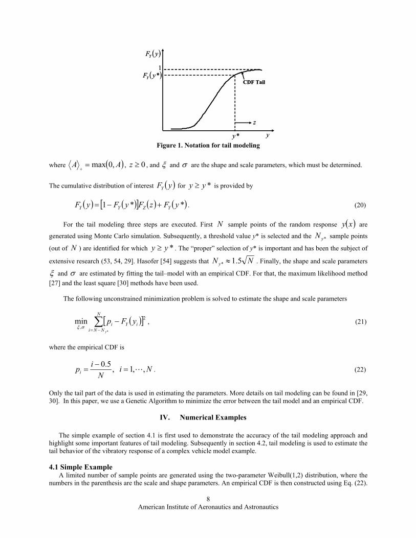
Let ( )xy be the system response. If x is randomly distributed, y will also be randomly distributed. If y* is a large threshold of y (see Fig. 1), the generalized Pareto distribution (GPD) provides a general approximation of the conditional distribution ( )zFZ of the exceedance *yyz −= for the region *yy ≥ . For a large value of y*, the
distribution ( )zFZ , conditioned upon *yy ≥ (i.e. z>0) is provided as follows, based on the extreme value theory [28]
( )
=
−−
≠+−=
−
+
0exp1
0111
ξσ
ξσξ ξ
ifz
ifzzFZ , (19)
American Institute of Aeronautics and Astronautics
8
( )yFY
y
( )*yFY
*y
z
1
CDF Tail
( )yFY
y
( )*yFY
*y
z
1
CDF Tail
Figure 1. Notation for tail modeling
where ( )AA ,0max=
+, 0≥z , and ξ and σ are the shape and scale parameters, which must be determined.
The cumulative distribution of interest ( )yFY for *yy ≥ is provided by
( ) ( )[ ] ( ) ( )**1 yFzFyFyF YZYY +−= . (20)
For the tail modeling three steps are executed. First N sample points of the random response ( )xy are
generated using Monte Carlo simulation. Subsequently, a threshold value y* is selected and the *yN sample points
(out of N ) are identified for which *yy ≥ . The “proper” selection of y* is important and has been the subject of
extensive research (53, 54, 29]. Hasofer [54] suggests that NN y 5.1* ≈ . Finally, the shape and scale parameters
ξ and σ are estimated by fitting the tail–model with an empirical CDF. For that, the maximum likelihood method [27] and the least square [30] methods have been used.
The following unconstrained minimization problem is solved to estimate the shape and scale parameters
( )[ ]∑−=
−N
NNiiYi
y
yFp*
2
,min
σξ, (21)
where the empirical CDF is
NiN
ipi ,,1,5.0L=
−= . (22)
Only the tail part of the data is used in estimating the parameters. More details on tail modeling can be found in [29, 30]. In this paper, we use a Genetic Algorithm to minimize the error between the tail model and an empirical CDF.
IV. Numerical Examples The simple example of section 4.1 is first used to demonstrate the accuracy of the tail modeling approach and highlight some important features of tail modeling. Subsequently in section 4.2, tail modeling is used to estimate the tail behavior of the vibratory response of a complex vehicle model example. 4.1 Simple Example A limited number of sample points are generated using the two-parameter Weibull(1,2) distribution, where the numbers in the parenthesis are the scale and shape parameters. An empirical CDF is then constructed using Eq. (22).
American Institute of Aeronautics and Astronautics
9
It is expected that as we increase the number of generated sample points, the empirical CDF will be approaching the actual CDF of the Weibull(1,2) distribution. As explained in the previous section, the tail modeling can estimate the upper part of the CDF for values larger than a threshold value ∗y (see Fig. 1). If the CDF value of *yN points with
∗∗∗ ≤≤ yyy is known, the tail model can extrapolate for ∗∗> yy providing therefore, an estimation of the tail behavior. We will demonstrate that the tail model can provide an accurate estimate of the upper tail of the distribution only if the CDF values of the *yN points are accurate.
The tail model is based on the extreme value theory which holds for a large threshold ∗y . However, the accurate
calculation of the CDF values for the *yN points becomes computationally demanding for large ∗y . There is
therefore, a trade-off between accuracy and efficiency depending on the threshold ∗y . Fig. 2 compares the
1 1.5 2 2.5 3 3.5 40.85
0.9
0.95
1
x
CD
F
Empirical CDFTail ModelWeibull(1,2)
Displacement (mm)1 1.5 2 2.5 3 3.5 4
0.85
0.9
0.95
1
x
CD
F
Empirical CDFTail ModelWeibull(1,2)
Displacement (mm)
Figure 2. Accuracy of tail model for 10,000 sample points
Figure 3. Accuracy of tail model for 100,000 sample points
upper part of the Weibull(1,2) distribution with the tail model. First, 10,000 sample points are generated from the Weibull(1,2) distribution. The shape and scale parameters ξ and σ , respectively of the tail model are then
estimated using *yN =50 points from the 10,000 points, such that ( )85.01−∗ = Fy and ( )9.01−∗∗ = Fy . Some of
the *yN points are indicated with squares, and labeled “Empirical CDF” points. The chosen ∗y and ∗∗y can practically provide a compromise between accuracy of the tail model and computational efficiency in calculating the corresponding CDF values of 0.85 and 0.9. Because only 10,000 sample points are generated, the empirical CDF between ∗y and ∗∗y is not very accurate although it is not apparent in Fig. 2. The tail model therefore, does not provide an accurate representation of the Weibull(1,2) CDF for large values of y (see Fig. 2). In Fig. 3, we used 100,000 sample points instead of 10,000
and the tail model is much more accurate due to better accuracy of the empirical CDF between ( )85.01−∗ = Fy
and ( )9.01−∗∗ = Fy . In Fig. 4, different samples of 100,000 points each, were generated from the Weibull(1,2) distribution, and the tail model was constructed similarly to Fig.3. We observe considerable differences in the tail approximation because of accuracy differences of the empirical CDF between ∗y and ∗∗y . It is therefore, important in tail modeling to use very accurate empirical CDF values. This can be only achieved if we perform a finite number of reliability analyses to calculate the actual CDF values between ∗y and ∗∗y instead of relying on the empirical CDF of Eq. (22).
1 1.5 2 2.5 3 3.5 40.85
0.9
0.95
1
x
CD
F
Empirical CDFTail ModelWeibull(1,2)
Displacement (mm)1 1.5 2 2.5 3 3.5 4
0.85
0.9
0.95
1
x
CD
F
Empirical CDFTail ModelWeibull(1,2)
Displacement (mm)
American Institute of Aeronautics and Astronautics
10
1 1.5 2 2.5 3 3.5 40.85
0.9
0.95
1
x
CD
F
Weibull(1,2)Tail Model
Displacement (mm)1 1.5 2 2.5 3 3.5 4
0.85
0.9
0.95
1
x
CD
F
Weibull(1,2)Tail Model
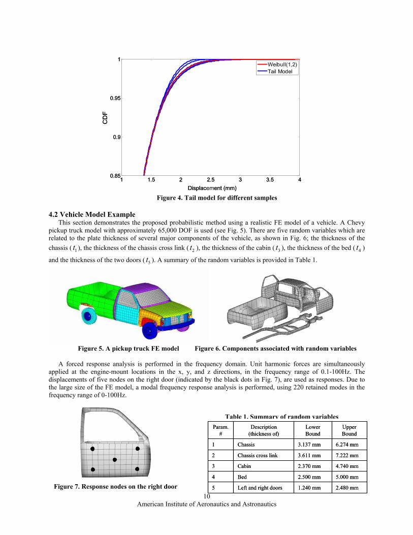
Displacement (mm) Figure 4. Tail model for different samples 4.2 Vehicle Model Example This section demonstrates the proposed probabilistic method using a realistic FE model of a vehicle. A Chevy pickup truck model with approximately 65,000 DOF is used (see Fig. 5). There are five random variables which are related to the plate thickness of several major components of the vehicle, as shown in Fig. 6; the thickness of the chassis ( 1t ), the thickness of the chassis cross link ( 2t ), the thickness of the cabin ( 3t ), the thickness of the bed ( 4t )
and the thickness of the two doors ( 5t ). A summary of the random variables is provided in Table 1.
Figure 5. A pickup truck FE model Figure 6. Components associated with random variables
A forced response analysis is performed in the frequency domain. Unit harmonic forces are simultaneously
applied at the engine-mount locations in the x, y, and z directions, in the frequency range of 0.1-100Hz. The displacements of five nodes on the right door (indicated by the black dots in Fig. 7), are used as responses. Due to the large size of the FE model, a modal frequency response analysis is performed, using 220 retained modes in the frequency range of 0-100Hz.
Table 1. Summary of random variables
Figure 7. Response nodes on the right door
2.480 mm1.240 mmLeft and right doors5
5.000 mm2.500 mmBed4
4.740 mm2.370 mmCabin3
7.222 mm3.611 mmChassis cross link2
6.274 mm3.137 mmChassis1
UpperBound
LowerBound
Description(thickness of)
Param.#
2.480 mm1.240 mmLeft and right doors5
5.000 mm2.500 mmBed4
4.740 mm2.370 mmCabin3
7.222 mm3.611 mmChassis cross link2
6.274 mm3.137 mmChassis1
UpperBound
LowerBound
Description(thickness of)
Param.#
American Institute of Aeronautics and Astronautics
11
0.2 0.22 0.24 0.26 0.28 0.30.85
0.9
0.95
1
x
CD
F
Empirical CDFLower Confidence LimitUpper Confidence LimitTail Model
0.2 0.22 0.24 0.26 0.28 0.30.85
0.9
0.95
1
x
CD
F
Empirical CDFLower Confidence LimitUpper Confidence LimitTail Model
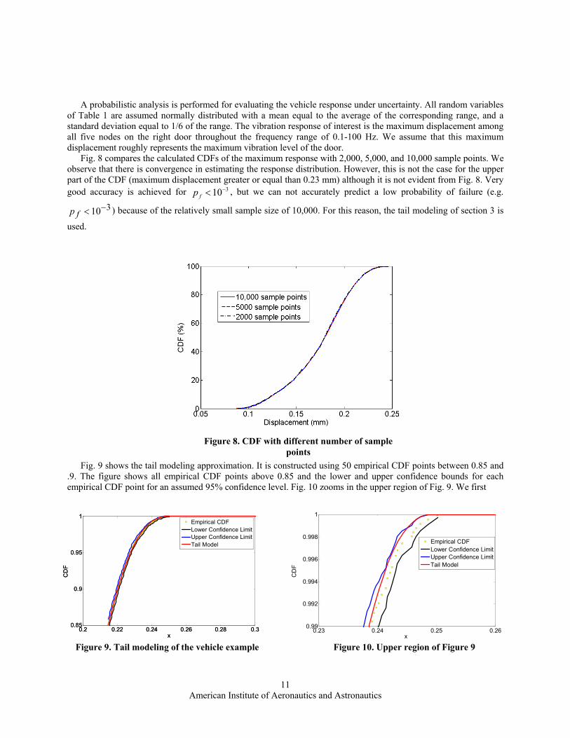
A probabilistic analysis is performed for evaluating the vehicle response under uncertainty. All random variables of Table 1 are assumed normally distributed with a mean equal to the average of the corresponding range, and a standard deviation equal to 1/6 of the range. The vibration response of interest is the maximum displacement among all five nodes on the right door throughout the frequency range of 0.1-100 Hz. We assume that this maximum displacement roughly represents the maximum vibration level of the door.
Fig. 8 compares the calculated CDFs of the maximum response with 2,000, 5,000, and 10,000 sample points. We observe that there is convergence in estimating the response distribution. However, this is not the case for the upper part of the CDF (maximum displacement greater or equal than 0.23 mm) although it is not evident from Fig. 8. Very good accuracy is achieved for 310−<fp , but we can not accurately predict a low probability of failure (e.g.
310−<fp ) because of the relatively small sample size of 10,000. For this reason, the tail modeling of section 3 is
used.
Fig. 9 shows the tail modeling approximation. It is constructed using 50 empirical CDF points between 0.85 and
.9. The figure shows all empirical CDF points above 0.85 and the lower and upper confidence bounds for each empirical CDF point for an assumed 95% confidence level. Fig. 10 zooms in the upper region of Fig. 9. We first
Figure 9. Tail modeling of the vehicle example Figure 10. Upper region of Figure 9
Figure 8. CDF with different number of sample points
0.23 0.24 0.25 0.260.99
0.992
0.994
0.996
0.998
1
x
CD
F
Empirical CDFLower Confidence LimitUpper Confidence LimitTail Model
American Institute of Aeronautics and Astronautics
12
observe that the tail model extrapolates the empirical CDF between 0.85 and 0.9 providing a decent approximation of the right tail PDF which follows the trend of the empirical CDF points. Also, the tail model is within the error bounds of the empirical CDF. Assuming that the empirical CDF points between 0.85 and 0.9 are accurate, we expect the tail model to provide an accurate extrapolation to high CDF values. Current research concentrates on the accurate calculation of the empirical CDF values between 0.85 and 0.9 using a probabilistic re-analysis method [55] which allows us to calculate the empirical CDF for different mean values of the plate thicknesses using a single Monte Carlo simulation. Furthermore, we are developing an RBDO process which combines deterministic and probabilistic re-analyses with tail modeling.
References 1 Madsen, H. O., Krenk, S., and Lind N. C., Methods of Structural Safety, Prentice-Hall, Inc. 1986. 2 Melchers, R. E., Structural Reliability Analysis and Prediction, John Wiley & Sons, 2001. 3 Moses F., “Probabilistic Analysis of Structural Systems” Probabilistic Structural Mechanics Handbook:
Theory and Industrial Applications, edited by C. Raj Sundararajan Chapman & Hall, 166-187, 1995. 4 Frangopol, D. M., “Reliability-Based Optimum Structural Design” Probabilistic Structural Mechanics
Handbook: Theory and Industrial Applications, edited by C. Raj Sundararajan Chapman & Hall, 352-387, 1995. 5 Royset, J. O., Der Kiureghian, A., and Polak, E., “Reliability-Based Optimal Design of Series Structural
Systems,” Journal of Engineering Mechanics, 127(6), 607-614, 2001. 6 Wang, L., Grandhi, R. V., and Hopkins, D. A., “Structural Reliability Optimization Using an Efficient Safety
Index Calculation Procedure,” International Journal for Numerical Methods in Engineering, 38, 1721-1738, 1995. 7 Ba-abbad, M. A. Kapania, R. K., and Nikolaidis, E., “Reliability-based Structural Optimization of an Elastic-
plastic Beam,” AIAA Journal, 41(8), 1573-1582, 2003. 8 Ayyub, B., and Mccuen, R., “Simulation-Based Reliability Methods” Probabilistic Structural Mechanics
Handbook: Theory and Industrial Applications, edited by C. Raj Sundararajan, Chapman & Hall, 53-69, 1995. 9 Olsson A. M. J., Sandberg G. E., and Dahlblom, O., “On Latin Hypercube Sampling for Structural Reliability
Analysis,” Structural Safety, 25, 47-68, 2003. 10 Fishman, G. S., Monte Carlo: Concepts, Algorithms, and Applications, Springer, 1996. 11 Moony, C. Z., Monte Carlo Simulation, Sage Publications, 1997. 12 Haldar, A., and Mahadevan, S., “First and Second Order Reliability Methods,” Probabilistic Structural
Mechanics Handbook: Theory and Industrial Applications, edited by C. Raj Sundararajan Chapman & Hall, 27-52, 1995.
13 Nikolaidis, E., and Burdisso, R., “Reliability Based Optimization: a Safety Index Approach,” Computers and Structures, 28(6), 781-788, 1988.
14 Der Kiureghian, A., “The Geometry of Random Vibrations and Solutions by FROM and SORM,” Probabilistic Engineering Mechanic, 15, 81-91, 2000.
15 Wu, Y. T., Millwater, H. R., and Cruse, T. A., “Advanced Probabilistic Structural Analysis Method for Implicit Performance Functions,” AIAA Journal, 28(9), 1663-1669, 1990.
16 Tandjiria, V., Teh C. I., and Low, B. K., “Reliability Analysis of Laterally Loaded Piles Using Response Surface Methods,” Structural Safety, 22, 335-355, 2000.
17 Krishnamurthy, T., and Romero, V. J., “Construction of Response Surface with Higher Order Continuity and its Application to Reliability Engineering,” 43rd AIAA/ASME/ASCE/AHS/ASC Structures, Structural Dynamics, and Materials Conference, Non-Deterministic Approaches Forum, Denver, CO., AIAA 2002-1466, 2002.
American Institute of Aeronautics and Astronautics
13
18 Gayton, N., Bourinet J. M., and Lamaire M., “CQ2RS: A New Statistical Approach to the Response Surface Method for Reliability Analysis,” Structural Safety, 25, 99-121, 2003.
19 Burton S. A., and Hajela, P., “Variable Complexity Reliability-Based Optimization with Neural Network Augmentation,” 43rd AIAA/ASME/ASCE/AHS/ASC Structures, Structural Dynamics, and Materials Conference and Exhibit, Non-Deterministic Approaches Forum, Denver, CO, AIAA 2002-1474, 2002.
20 Papadrakakis, M., and Lagaros, N. D., “Reliability-Based Structural Optimization Using Neural Networks and Monte-Carlo Simulation,” Computer Methods in Applied Mechanics and Engineering, 191, 3491-3507, 2002.
21 Youn, Byeng D. and Choi, K. K., “A New Response Surface Methodology for Reliability-Based Design Optimization (RBDO),” Computers & Structures, 82(2), 241-256, 2004.
22 Chandu S. V. L., and Grandhi R. V., “General Purpose Procedure for Reliability Based Structural Optimization Under Parametric Uncertainties” Advances in Engineering Software, 23, 7-14, 1995.
23 Grandhi, R. V., and Wang, L., “Reliability-based Structural Optimization Using Improved Two Point Adaptive Nonlinear Approximations,” Finite Elements in Analysis and Design, 29, 35-48, 1998.
24 Qu, X., and Haftka, R. T., “A Reliability-based Design Optimization Using Probabilistic Safety Factor,” 44th AIAA/ASME/ASCE/AHS/ASC Structures, Structural Dynamics and Materials Conference, AIAA 2003-1657, 2003.
25 Zhang, G., Mourelatos, Z. P., and Nikolaidis, E., “An Efficient Re-Analysis Methodology for Probabilistic Vibration of Complex Structures,” 48th AIAA/ASME/ASCE/AHS/ASC Structures, Structural Dynamics, and Materials Conference, Honolulu, Hawaii, AIAA 2007-1963, 2007.
26 Ghanem, R., and Spanos, P. D., Stochastic Finite Elements: A Spectral Approach, Springer-Verlag, NY, 1991.
27 Prescott, P., and Walden, A., “Maximum Likelihood Estimation of the Parameters of the Generalized Extreme-Value Distribution,” Biometrika, 67(3), 723-724, 1980.
28 Castillo, E., Extreme Value Theory in Engineering, Academic Press, San Diego, CA, 1988. 29 Caers, J., and Maes, M., “Identifying Tails, Bounds, and End-Points of Random Variables,” Structural Safety,
20, 1-23, 1998. 30 Kim, N.-H., and Ramu, P., “Tail Modeling in Reliability-Based Design Optimization for Highly Safe
31 Abu Kasim, A. M., “Topping, Static Re-analysis: A Review,” ASCE Journal of Structural Engineering, 113, 1029-1045, 1987.
32 Arora, J. S., “Survey of Structural Re-analysis Techniques,” ASCE Journal of Structural Engineering, 102, 783-802, 1976.
33 Barthelemy, J-F.M., and Haftka, R. T., “Approximation Concepts for Optimum Structural Design - A Review,” Struct. Optim., 5, 129-144, 1993.
34 Balmes, E., “Optimal Ritz Vectors for Component Mode Synthesis using the Singular Value Decomposition,” AIAA Journal, 34(6), 1256–1260, 1996.
35 Balmes, E., Ravary, F., and Langlais, D., “Uncertainty Propagation in Modal Analysis,” Proceedings of IMAC-XXII: A Conference & Exposition on Structural Dynamics, Dearborn, MI., 2004.
36 Zhang, G., Castanier, M. P., and Pierre, C., “Integration of Component-Based and Parametric Reduced-Order Modeling Methods for Probabilistic Vibration Analysis and Design,” Proceedings of the Sixth European Conference on Structural Dynamics, Paris, France, 2005.
37 Zhang, G., “Component-Based and Parametric Reduced-Order Modeling Methods for Vibration Analysis of Complex Structures,” Ph.D thesis, The University of Michigan, Ann Arbor, MI, 2005.
American Institute of Aeronautics and Astronautics
14
39 Kirsch, U., “Design-Oriented Analysis of Structures – A unified Approach,” ASCE Journal of Engineering Mechanics, 129, 264-272, 2003.
40 Kirsch, U., “A Unified Re-analysis Approach for Structural Analysis, Design and Optimization,” Structural and Multidisciplinary Optimization, 25, 67-85, 2003.
41 Chen, S. H., and Yang, X. W., “Extended Kirsch Combined Method for Eigenvalue Re-analysis,” AIAA Journal, 38, 927-930, 2000.
42 Kirsch, U., “Approximate Vibration Re-analysis of Structures,” AIAA Journal, 41, 504-511, 2003. 43 Kirsch, U., and Bogomolni, M., “Procedures for Approximate Eigenproblem Re-analysis of Structures,”
Intern. J. for Num. Meth. Engrg., 60, 1969-1986, 2004. 44 Kirsch, U., and Bogomolni, M., “Error Evaluation in Approximate Re-analysis of Structures,” Structural
Optimization, 28, 77-86, 2004. 45 Rong, F., et al., “Structural Modal Re-analysis for Topological Modifications with Extended Kirsch Method,”
Comp. Meth. in Appl. Mech. and Engrg., 192, 697-707, 2003. 46 Chen, S. H., et al., “Comparison of Several Eigenvalue Re-analysis Methods for Modified Structures,”
Structural Optimization, 20, 253-259, 2000. 47 Fang, K.-T., Runze, L., and Sudjianto, A., Design and Modeling for Computer Experiments, Chapman &
Hall/CRC, Taylor & Francis Group, Boca Raton, FL, 2006. 48 Haldar, A. and Mahadevan, S., Probability, Reliability and Statistical Methods in Engineering Design, John
Wiley & Sons, Inc., 2000. 49 Pearson, K., “Contributions to the Mathematical Theory of Evolution. II Skew Variations in Homogeneous
Material,” Philosophical Transactions of the Royal Society of London, Series A, 186, 343-414, 1895. 50 Johnson, N. L., and Kotz, S., Distributions in Statistics: Continuous Univariate Distributions, Houghton
Miffin Co., Boston, 1970. 51 Johnson, N. L., and Kotz, S., Distributions in Statistics: Continuous Multivariate Distributions, John Wiley &
Sons, Inc., New York, 1972. 52 Maes, M. A., and Breitung, K., “Reliability-Based Tail Estimation,” Proceedings IUTAM Symposium on
Probabilistic Structural Mechanics (Advances in Structural Reliability Methods), San Antonio, TX, 335-346, 1993. 53 Boos, D., “Using Extreme Value Theory to Estimate Large Percentiles,” Technometrics, 26(1), 33-39, 1984. 54 Hasofer, A., “Non-Parametric Estimation of Failure Probabilities,” Mathematical Models for Structural
Reliability, Eds. F. Casciati, and B. Roberts, CRC Press, Boca Raton, FL, 195-226, 1996. 55 Zhang, G., Nikolaidis, E., and Mourelatos, Z. P., “An Efficient Re-Analysis Methodology for Probabilistic
Vibration of Large-Scale Structures,” Proceedings, ASME International Design Engineering Technical Conferences, New York, NY, DETC2008-49156, 2008.