[American Institute of Aeronautics and Astronautics 49th AIAA/ASME/ASCE/AHS/ASC Structures,...

American Institute of Aeronautics and Astronautics

1

Multilevel Decomposition Based Non-Deterministic Design

Optimization

Varun Sakalkar1 and Prabhat Hajela2

Mechanical, Aerospace and Nuclear Engineering

Rensselaer Polytechnic Institute, Troy, New York 12180

The paper presents a methodology for non-deterministic design optimization of

hierarchically coupled structural systems. Deterministic multilevel decomposition based design

formulations for such systems have been modified to incorporate the presence of uncertainty

in both the problem parameters, and in design variables at various levels of a multilevel

hierarchical system. These formulations not only allow for robust design solution strategies,

but also provide a mechanism for tracking the propagation of uncertainty in such hierarchical

systems. For uncertain design variables distributed across several subsystems, an iterative

problem formulation is proposed. A widely used numerical example based on the design of a

portal frame is used to illustrate the problem complexities in this class of design problems, and

to demonstrate the effectiveness of the proposed solution techniques.

Nomenclature

Xk kth subsystem level design variable

yk kth subsystem level design variable

gj jth behavioral constraint

p System level design parameters

~ Signifies a random variate or a function of random variables for e.g. x identifies x as a random

variable

kΩ Cumulative constraint for the kth subsystem

SS(k) kth subsystem

Pf Probability of failure

µ Sub/super script; signifies the mean of the associated random variate

σ Subscript; signifies the standard deviation of the associated random variate

l, u Superscript; lower and upper bounds for the associated variable

k Subscript; kth subsystem

ρ Scale factor for the cumulative constraint

Aj, Ij Cross-section area and moment of inertia respectively of a jth beam

allow Sub/super script; allowable value of associated variable

gs System level set of constraint

I. Introduction

Decomposition-based design strategies have been explored in a number of recent studies as a solution to large-

scale coupled problems, wherein the original problem is decomposed into a number of smaller, more tractable sub

problems1. Not only do the smaller sub-problems provide for easier solutions to the design problem but also

facilitate a better understanding of the problem domain. In some instances, decomposition would also allow for

parallel processing and therefore speedier solutions to the design problem. Traditional decomposition strategies fall

into three principal categories - object decomposition, aspect decomposition, and sequential decomposition. Object

decomposition partitions a system on the basis of the physical elements of the system. In multidisciplinary design of

an airplane, the design of the power plant and the airframe could be treated as decoupled problems by explicitly

accounting for the interactions between the two domains. Aspect decomposition seeks to partition the problem

based on the physics of the system. The third category, sequential decomposition, partitions the problem in a manner

1 Doctoral Candidate, Department of Mechanical, Aerospace and Nuclear Engineering, AIAA Student member. 2 Professor, Department of Mechanical, Aerospace and Nuclear Engineering, AIAA Fellow.

49th AIAA/ASME/ASCE/AHS/ASC Structures, Structural Dynamics, and Materials Conference <br> 16t7 - 10 April 2008, Schaumburg, IL

AIAA 2008-2221

Copyright © 2008 by the American Institute of Aeronautics and Astronautics, Inc. All rights reserved.


2

best suited to the flow of design information. The structure of typical design problems after decomposition may

either be hierarchical or non-hierarchical, depending upon the coupling between the decomposed sub problems. The

coupling may be hierarchical, where it is possible to identify distinct tree-like patterns of interaction or, no obvious

hierarchy may exist, and there may be multiple one or two-way couplings among sub problems.

In order that the optimal solution to the original design problem is obtained through solutions of several smaller

sized sub problems, solution coordination is necessary to account for any interactions among the decomposed sub

problems. The ways in which such interactions are taken into account is the very essence of the many

decomposition-based methods that have been proposed in the literature2-5. Most of these studies have been limited to

problems where the analysis and design problem was strictly deterministic. There is recent literature that has

addressed fundamental issues related to including the effects of uncertainty in such design problems6, 7.

Among the fundamental problems and issues that must be addressed in nondeterministic design problems, the

following need special consideration.

- How do uncertainties propagate in coupled hierarchical systems?

- How should the problem formulation for design optimization change in the presence of uncertainties?

- What special considerations should be given to computational requirements of the design problem in the

presence of uncertainties?

These are issues central to the design of any coupled multidisciplinary system. Similar issues are also

encountered in the multiscale analysis of structures and materials systems, where analysis models span length scales

ranging from the nano to the macro level; uncertainty in analysis at any scale propagates into other length scales,

rendering the coupled analysis as a computationally expensive process that is difficult to insert within a design

framework. An illustration of this complexity is available in a nondeterministic damage analysis of laminated

composite materials using the Transformation Field Analysis (TFA) approach8.

Reliability analysis for multidisciplinary systems using probabilistic information has been examined in previous

efforts9, 10. Analytical approaches such as FOSM, AVFOSM, FORM and SORM, as well as the use of Monte Carlo

simulations are well understood, with additional research in progress11-15. Design problems examined in this context

have not been applied in a meaningful manner to large-scale coupled systems, including those that are amenable to a

decomposition based design approach.

The focus of present paper is to look at the category of hierarchically partitioned or decomposed design

problems. To facilitate this study, the issue of uncertainty inclusion in the design process will be examined in the

context of a simple two-level design problem. Design formulations that have been used in the solution of such

problems will be examined from the nondeterministic perspective, and reformulated so as to develop appropriate

solution strategies that are both computationally efficient and numerically robust. The following subsection

examines a generic decomposition based design problem formulation that serves as a template for hierarchical

decomposition.

II. Decomposition Formulations:

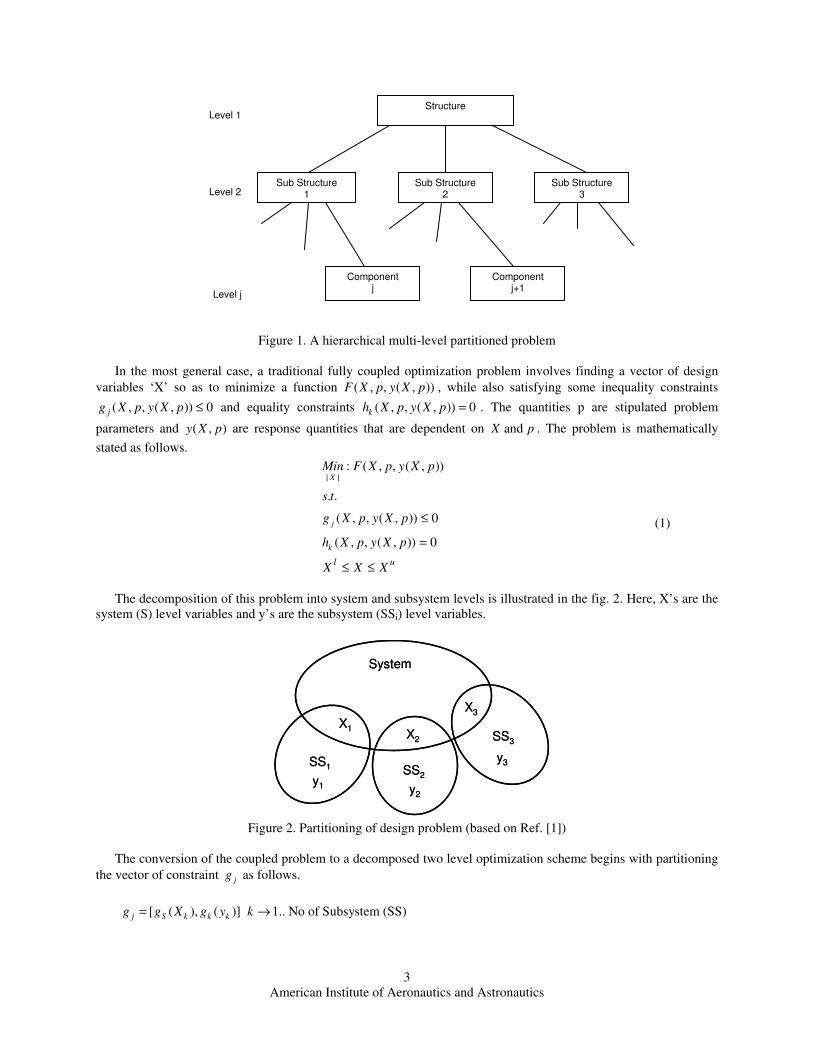
A generic multilevel, partitioned structural design problem is schematically shown in Figure 1. The structure is

decomposed into sub structures, each one of which may be subjected to further hierarchical decomposition. The top-

down or bottom-up flow of information in a hierarchical pattern has been studied in the context of design

decomposition. System level design objectives are met by formulating design problems at various levels of the

decomposed problem, and propagating design information from one level to another.


3

Figure 1. A hierarchical multi-level partitioned problem

In the most general case, a traditional fully coupled optimization problem involves finding a vector of design

variables ‘X’ so as to minimize a function ( , , ( , ))F X p y X p , while also satisfying some inequality constraints

( , , ( , )) 0jg X p y X p ≤ and equality constraints ( , , ( , )) 0kh X p y X p = . The quantities p are stipulated problem

parameters and ( , )y X p are response quantities that are dependent on X and p . The problem is mathematically

stated as follows.

[ ]

: ( , , ( , ))

. .

( , , ( , )) 0

( , , ( , )) 0

X

j

k

l u

Min F X p y X p

s t

g X p y X p

h X p y X p

X X X

≤

=

≤ ≤

(1)

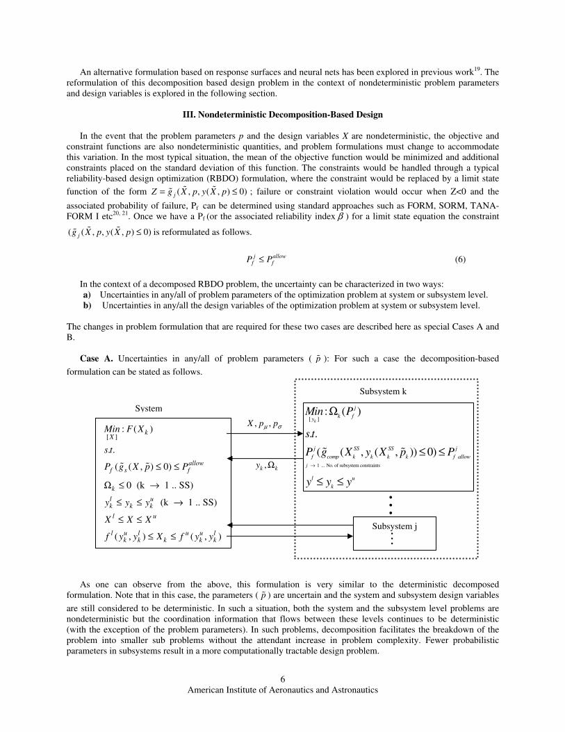
The decomposition of this problem into system and subsystem levels is illustrated in the fig. 2. Here, X’s are the

system (S) level variables and y’s are the subsystem (SSi) level variables.

Figure 2. Partitioning of design problem (based on Ref. [1])

The conversion of the coupled problem to a decomposed two level optimization scheme begins with partitioning

the vector of constraint jg as follows.

[ ( ), ( )] 1.. No of Subsystem (SS)j S k k kg g X g y k= →

Structure

Sub Structure 1

Sub Structure 2

Level 1

Sub Structure 3

Component j

Component j+1

Level 2

Level j

System

X1X2

X3

SS1 SS2

SS3

y1 y2

y3

System

X1X2

X3

SS1 SS2

SS3

y1 y2

y3


4

Here, ( )S kg X contains the system level constraints and remaining ( )k kg y are subsystem level constraints. The

kth subsystem level optimization problem is typically formulated as follows:

[ ]: ( )

. .

( , ( , )) 0

k

k ky

SS SScomp k k k k

l uk

Min g

s t

g X y X p

y y y

Ω

=

≤ ≤

(2)

Here ( )k kgΩ is a cumulative measure of constraint violation in the sub-system and the cumulative constraint

function16 kΩ has been used in this context in previous work. The expression for ( )k kgΩ is as follows.

1ln exp( )k j

j

gρρ

Ω =

∑ (3)

Where, the factor ρ determines the extent to which a constraint contributes to ( )k kgΩ .

In eqn. 2 ( , ( , ))comp k k k kg X y X p represents compatibility constraints to ensure the invariance of the system level

variables SSkX with respect to the subsystem level variables ky .

Each subsystem level optimization provides the optimum ( )k kgΩ and optimal design variables ky and their

respective sensitivities with respect to SSkX and kp as follows: ( , , , )k k k k

SS SSk k k k

y y

X p X p

∂Ω ∂Ω ∂ ∂

∂ ∂ ∂ ∂

This sensitivity information is used at the system level to formulate the optimization problem at this level of

design as follows1.

[ ]

0

1

0

1

: ( )

. .

0

0 (k 1 .. SS)

(k 1 .. SS)

( , ) ( , )

kX

S

SSk

k k k

k k

SSl ukk k k k k

k k

l u

l u l u u lk k k k k

Min F X

s t

g

XX

yy y y X y

X

X X X

f y y X f y y

=

=

≤

∂ΩΩ = Ω + ∆ ≤ →

∂

∂≤ = + ∆ ≤ →

∂

≤ ≤

≤ ≤

∑

∑

(4)

Eqn. 4 at the system level relates the system level variable and parameters to the subsystem level variables using

the optimum problem parameter sensitivity information17, 18. In the above, 0kΩ and 0

ky are the values of the kth

subsystem cumulative constraint and design variables respectively, at the start of the new system level optimization

problem.

As can be seen the approximation of kΩ and ky available at the system level is only as good as the first order

sensitivity information. Typically, tight move limits would have to be imposed at the system level to ensure that the

quality of the approximation would justify its use at the system level.


5

The use of the linear approximation of subsystem level constraints and design variables at the system level

eliminates a recursive calculation of the subsystem optimization loop for each new value of the system level design

variables. This can be viewed as a “greedy” implementation of decomposition process, wherein some of the effort

assigned to the sub problem level design is actually done at the system level. Although this results in saving of

computational resources, it generally results in some undesirable solution attributes.

a) The optimization typically leads to a far more conservative design compared to the all-in-one solution,

more so if the initial starting point is far away from the optimum;

b) To extend this formulation to the non deterministic case would involve calculating the second order

derivatives of the optimal solutions with respect to the random variables (details in Section 3.1) which can

be numerically inaccurate. This formulation would be, therefore, infeasible in a probabilistic framework.

The problem can be circumvented by replacing the linearized constraints with ( )0 0 k kΩ = Ω ≤ and the explicit

dependence of the optima 0kΩ on the coordination level or system level variables is achieved by solving each

subsystem optimization loop for each iteration of the system level optimization. This approach not only ensures

more robust system level optima but it can also be extended to non deterministic problems with minor

modifications. The details of the modified system level deterministic formulation are shown below:

( )( )

[ ]

0

0

( )

. .

0

0 (k 1 .. SS)

(k 1 .. SS)

( , ) ( , )

kX

s

k k

l uk k k

l u


Min F X

s t

g

y y y

X X X

f y y X f y y

≤

Ω = Ω ≤ →

≤ ≤ →

≤ ≤

≤ ≤

(5)

The important change to be noted here is that for the deterministic decomposition proposed above, the sensitivity

of the optimal subsystem solution is not required (although, this would be required in the non deterministic case).

The sequence of design steps is illustrated in the following flowchart.

[ ]: ( )

. .

( , ( , )) 0

k

k ky

SS SS

comp k k k k

l u

k

Min g

s t

g X y X p

y y y

Ω

≤

≤ ≤

kth Subsystem

System Level Problem:

( )

( )

[ ]

0

0

: ( )

. .

0 (k 1 .. SS)

(k 1 .. SS)

( , ) ( , )

kX

k k

l u

k k k

l u

l u l u u l

k k k k k

Min F X

s t

y y y

X X X

f y y X f y y

Ω = Ω ≤ →

≤ ≤ →

≤ ≤

≤ ≤

System level

variables Xk

kth subsystem optima and

optimal solution

kth system level optimization iterationXk

Xk+1


6

An alternative formulation based on response surfaces and neural nets has been explored in previous work19. The

reformulation of this decomposition based design problem in the context of nondeterministic problem parameters

and design variables is explored in the following section.

III. Nondeterministic Decomposition-Based Design

In the event that the problem parameters p and the design variables X are nondeterministic, the objective and

constraint functions are also nondeterministic quantities, and problem formulations must change to accommodate

this variation. In the most typical situation, the mean of the objective function would be minimized and additional

constraints placed on the standard deviation of this function. The constraints would be handled through a typical

reliability-based design optimization (RBDO) formulation, where the constraint would be replaced by a limit state

function of the form ( , , ( , ) 0)jZ g X p y X p= ≤ ; failure or constraint violation would occur when Z<0 and the

associated probability of failure, Pf can be determined using standard approaches such as FORM, SORM, TANA-

FORM I etc20, 21. Once we have a Pf (or the associated reliability index β ) for a limit state equation the constraint

( ( , , ( , ) 0)jg X p y X p ≤ is reformulated as follows.

j allowf fP P≤ (6)

In the context of a decomposed RBDO problem, the uncertainty can be characterized in two ways:

a) Uncertainties in any/all of problem parameters of the optimization problem at system or subsystem level.

b) Uncertainties in any/all the design variables of the optimization problem at system or subsystem level.

The changes in problem formulation that are required for these two cases are described here as special Cases A and

B.

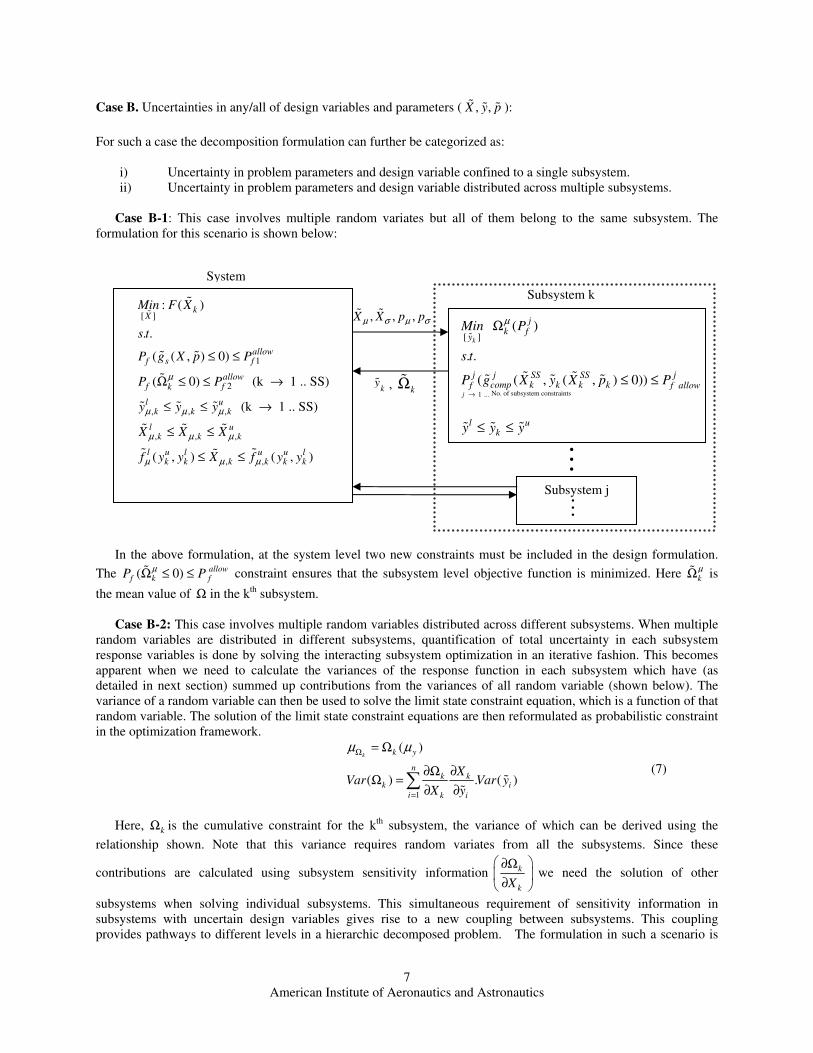
Case A. Uncertainties in any/all of problem parameters ( p ): For such a case the decomposition-based

formulation can be stated as follows.

As one can observe from the above, this formulation is very similar to the deterministic decomposed

formulation. Note that in this case, the parameters ( p ) are uncertain and the system and subsystem design variables

are still considered to be deterministic. In such a situation, both the system and the subsystem level problems are

nondeterministic but the coordination information that flows between these levels continues to be deterministic

(with the exception of the problem parameters). In such problems, decomposition facilitates the breakdown of the

problem into smaller sub problems without the attendant increase in problem complexity. Fewer probabilistic

parameters in subsystems result in a more computationally tractable design problem.

[ ]: ( )

. .

( ( , ) 0)

0 (k 1 .. SS)

(k 1 .. SS)

( , ) ( , )

kX

allowf s f

k

l uk k k

l u


Min F X

s t

P g X p P

y y y

X X X

f y y X f y y

≤ ≤

Ω ≤ →

≤ ≤ →

≤ ≤

≤ ≤

System

Subsystem k

, ,X p pµ σ

,k ky Ω

Subsystem j

1 ... No. of subsystem constraints

[ ]

: ( )

. .

( ( , ( , )) 0)

k

j

j

k fy

j SS SS j

f comp k k k k f allow

l u

k

Min P

s t

P g X y X p P

y y y

→

Ω

≤ ≤

≤ ≤


7

Case B. Uncertainties in any/all of design variables and parameters ( , ,X y p ):

For such a case the decomposition formulation can further be categorized as:

i) Uncertainty in problem parameters and design variable confined to a single subsystem.

ii) Uncertainty in problem parameters and design variable distributed across multiple subsystems.

Case B-1: This case involves multiple random variates but all of them belong to the same subsystem. The

formulation for this scenario is shown below:

In the above formulation, at the system level two new constraints must be included in the design formulation.

The ( 0) allow

f k fP PµΩ ≤ ≤ constraint ensures that the subsystem level objective function is minimized. Here k

µΩ is

the mean value of Ω in the kth subsystem.

Case B-2: This case involves multiple random variables distributed across different subsystems. When multiple

random variables are distributed in different subsystems, quantification of total uncertainty in each subsystem

response variables is done by solving the interacting subsystem optimization in an iterative fashion. This becomes

apparent when we need to calculate the variances of the response function in each subsystem which have (as

detailed in next section) summed up contributions from the variances of all random variable (shown below). The

variance of a random variable can then be used to solve the limit state constraint equation, which is a function of that

random variable. The solution of the limit state constraint equations are then reformulated as probabilistic constraint

in the optimization framework.

1

( )

( ) . ( )

k k y

nk k

k i

i k i

XVar Var y

X y

µ µΩ

=

= Ω

∂Ω ∂Ω =

∂ ∂∑

(7)

Here, kΩ is the cumulative constraint for the kth subsystem, the variance of which can be derived using the

relationship shown. Note that this variance requires random variates from all the subsystems. Since these

contributions are calculated using subsystem sensitivity information k

kX

∂Ω

∂ we need the solution of other

subsystems when solving individual subsystems. This simultaneous requirement of sensitivity information in

subsystems with uncertain design variables gives rise to a new coupling between subsystems. This coupling

provides pathways to different levels in a hierarchic decomposed problem. The formulation in such a scenario is

ky , kΩ

, , ,X X p pµ σ µ σ [ ]

1

2

, , ,

, , ,

, ,

: ( )

. .

( ( , ) 0)

( 0) (k 1 .. SS)

(k 1 .. SS)

( , ) ( , )

kX

allowf s f

allowf fk

l uk k k

l uk k k

l u l u u lk k k k k k

Min F X

s t

P g X p P

P P

y y y

X X X

f y y X f y y

µ

µ µ µ

µ µ µ

µ µ µ

≤ ≤

Ω ≤ ≤ →

≤ ≤ →

≤ ≤

≤ ≤

No. of subsystem constraints1 ...

[ ]

( )

. .

( ( , ( , ) 0))

k

j

jk f

y

j jj SS SScomp k k k kf f allow

l uk

Min P

s t

P g X y X p P

y y y

µ

→

Ω

≤ ≤

≤ ≤

Subsystem k

System

Subsystem j


8

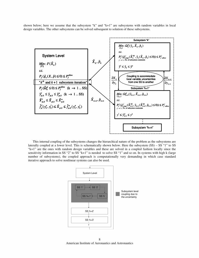
shown below; here we assume that the subsystem “k” and “k+1” are subsystems with random variables in local

design variables. The other subsystems can be solved subsequent to solution of these subsystems.

This internal coupling of the subsystems changes the hierarchical nature of the problem as the subsystems are

laterally coupled at a lower level. This is schematically shown below. Here the subsystem (SS) – SS “1” to SS

“k+1” are the ones with random design variables and these are solved in a coupled fashion locally since the

sensitivity information in SS “2” to SS “k+1” is needed to solve SS “1” and so on. In systems with high k (large

number of subsystems), the coupled approach is computationally very demanding in which case standard

iterative approach to solve nonlinear systems can also be used.

System Level

SS ‘1’ SS ‘2’

SS ‘k’SS ‘k+1’

SS ‘k+2’

SS ‘k+3’

Subsystem level

coupling due to

the uncertainty

[ ]

, , ,

, , ,

, ,

: ( )

. .

( ( , ) 0)

" and 1 subsystem iteration"

( 0) (k 1 .. SS)

(k 1 .. SS)

( , ) ( , )

kX

allow

f s f

th

allow

f k f

l u

k k k

l u

k k k

l u l u u l

k k k k k k

Min F X

s t

P g X p P

k k

P P

y y y

X X X

f y y X f y y

µ

µ µ µ

µ µ µ

µ µ µ

≤ ≤

+

Ω ≤ ≤ →

≤ ≤ →

≤ ≤

≤ ≤

System Level

[ ]

No. of subsystem constraints1..

: ( , , )

. .

( ( , ( , ) 0))

k

k k k ky

j j SS j


j

l u

k

Min y X p

s t

P g X y X p P

y y y

µ

→

Ω

≤ ≤

≤ ≤

1

1 1 1 1[ ]

1 1 1 1 No. of subsystem constraints1..

1

: ( , , )

. .

( ( , ( , ) 0))

k

k k k ky

j j SS SS j


j

l u

k

Min y X p

s t

P g X y X p P

y y y

µ

µ

++ + + +

+ + + +→

+

Ω

≤ ≤

≤ ≤

Subsystem “k”

Subsystem “k+1”

Coupling to accommodate local variable uncertainties

from one SS to another

,k k

X p

1 1,k kX p+ +

Subsystem “k+n”

k

k

X

y

∂

∂1

1

k

k

X

y

+

+

∂

∂

[ ]

, , ,

, , ,

, ,

: ( )

. .

( ( , ) 0)


( 0) (k 1 .. SS)

(k 1 .. SS)

( , ) ( , )

kX

allow

f s f

th

allow

f k f

l u

k k k

l u

k k k

l u l u u l

k k k k k k

Min F X

s t

P g X p P

k k

P P

y y y

X X X

f y y X f y y

µ

µ µ µ

µ µ µ

µ µ µ

≤ ≤

+

Ω ≤ ≤ →

≤ ≤ →

≤ ≤

≤ ≤

System Level

[ ]


: ( , , )

. .

( ( , ( , ) 0))

k

k k k ky

j j SS j


j

l u

k

Min y X p

s t

P g X y X p P

y y y

µ

→

Ω

≤ ≤

≤ ≤

1

1 1 1 1[ ]


1

: ( , , )

. .

( ( , ( , ) 0))

k

k k k ky

j j SS SS j


j

l u

k

Min y X p

s t

P g X y X p P

y y y

µ

µ

++ + + +

+ + + +→

+

Ω

≤ ≤

≤ ≤

Subsystem “k”

Subsystem “k+1”



,k k

X p

1 1,k kX p+ +

Subsystem “k+n”

[ ]

, , ,

, , ,

, ,

: ( )

. .

( ( , ) 0)


( 0) (k 1 .. SS)

(k 1 .. SS)

( , ) ( , )

kX

allow

f s f

th

allow

f k f

l u

k k k

l u

k k k

l u l u u l

k k k k k k

Min F X

s t

P g X p P

k k

P P

y y y

X X X

f y y X f y y

µ

µ µ µ

µ µ µ

µ µ µ

≤ ≤

+

Ω ≤ ≤ →

≤ ≤ →

≤ ≤

≤ ≤

System Level

[ ]

, , ,

, , ,

, ,

: ( )

. .

( ( , ) 0)


( 0) (k 1 .. SS)

(k 1 .. SS)

( , ) ( , )

kX

allow

f s f

th

allow

f k f

l u

k k k

l u

k k k

l u l u u l

k k k k k k

Min F X

s t

P g X p P

k k

P P

y y y

X X X

f y y X f y y

µ

µ µ µ

µ µ µ

µ µ µ

≤ ≤

+

Ω ≤ ≤ →

≤ ≤ →

≤ ≤

≤ ≤

System Level

[ ]


: ( , , )

. .

( ( , ( , ) 0))

k

k k k ky

j j SS j


j

l u

k

Min y X p

s t

P g X y X p P

y y y

µ

→

Ω

≤ ≤

≤ ≤

1

1 1 1 1[ ]


1

: ( , , )

. .

( ( , ( , ) 0))

k

k k k ky

j j SS SS j


j

l u

k

Min y X p

s t

P g X y X p P

y y y

µ

µ

++ + + +

+ + + +→

+

Ω

≤ ≤

≤ ≤

Subsystem “k”

Subsystem “k+1”



,k k

X p

1 1,k kX p+ +

Subsystem “k+n”

k

k

X

y

∂

∂1

1

k

k

X

y

+

+

∂

∂


9

3.1 Uncertainty propagation:

The various response functions in the above formulation are nonlinear functions of a set of independent variables

(x). If the variables x are random, the function ( )F x is also random. For a function ( )F x that is generally non-

linear, the mean and moment estimation of this function can be done using a mean value first order second moment

method. This method involves forming a first order Taylor’s series expansion of the function ( )F x about the current

design point, ixµ as follows:

1

( ) ( ) ( )i i

xi

n

x i x

i i

FF x F x

xµ

µ µ=

∂≈ + −

∂ ∑

(8)

Here n is the number of random variables.

The mean of the function is ( ) ( )ixF x F µ≈ and

1

( ( )) ( )

xi

n

i

i i

FVar F x Var x

xµ=

∂=

∂ ∑

(assuming ix to be independent

and normal in nature). For non-normal random variables, one must transform the variables into an equivalent normal

space (e.g. by doing a Rosenblatt transformation20, 22) before applying the above procedure.

In multilevel hierarchic optimization, the optimal solutions of the kth subsystem, kΩ and ky , are input to the

coordination or system level problem. The probability of failure ( 0)f kPµΩ ≤ required in the coordination level

problem would require evaluating the mean and variance of kΩ . These can be evaluated as follows:

1

( )

( ) . ( )

k k y

nk k

k i

i k i

XVar Var y

X y

µ µΩ

=

= Ω

∂Ω ∂Ω =

∂ ∂∑

(9)

Here k

kX

∂Ω

∂ is the sensitivity of the optimal solution to the problem parameters explained earlier and are obtained

for each subsystem optimization. The computation of the problem parameter sensitivity has been explored in

previous work17, 18. The approach proposed by Vanderplaats18 entails the solution of a secondary optimization

problem with the parameter sensitivities as design variables. The problem statement is as follows: *

*

*

: ( , ).

. .

( ). 0 1, 2,...

. 1

,

k

j

T k

Max y p S

s t

g y S j M

S S

yS

p p

µ

µ

µ

µ µ

∇Ω

∇ ≤ =

<

∂ ∂Ω ⇒ =

∂ ∂

(10)

and p are the problem parameters for which sensitivity is required. 'S' is the design variable vector for this

secondary optimization problem; the components of this vector represent the sensitivity of the optimal design

variables and the objective function to the problem parameters. The only requirement for this approach is that for the

parameter sensitivities to be valid, the active constraint set at the optimum must not change with the variations in the

problem parameters. With this in mind the solution of the above optimization problem gives us the vector S which

can then be used to compute the variance in the above eqn. 9.


10

IV. Pseudo code for the non deterministic decomposition based optimization

The methodology for multilevel optimization under uncertainty as described in previous section can be

summarized in the following steps for the various cases presented above:

Case A:

a) Initialize all the system level variables and propagate appropriate coupling variables to the subsystem. In

this case the design variables at the system or sub-system level may not be random in nature (eqn. 2).

b) Solve each subsystem level problem by using the probabilistic formulation of the constraints (eqn. 3).

c) Check for satisfaction of constraints at the coordination level and iterate.

Case B-1:

a) Initialize all the system level variables at their mean values.

b) Go to the lowest level in the hierarchy to compute characteristics that define the uncertainty in coupling

variables at that level and propagate that information to a higher level through the use of optimal sensitivity

analysis described in eqn. (10). Since the uncertainty is restricted to a single subsystem, the solution of this

subsystem (i.e. the subsystem optimal mean and standard deviation of design variables, additionally the

optimal mean and standard deviation of the subsystem objective function) can be propagated to the system

level formulation (as required in eqn. 4).

c) Calculate the probability of failure using the probabilistic characteristics derived in step – b above and

solve the limit state equations corresponding to a desired level of reliability. (eqn. 9)

d) Check for satisfaction of constraints and iterate.

Case B-2:

a) Initialize all the system level variables at their mean values.

b) Since the uncertain variables are distributed across different subsystems there is a need to solve these

subsystems in a coupled fashion (as described in section 3) to compute characteristics that define the

uncertainty in coupling variables in the individual subsystems. Propagate the subsystem level information

(i.e. the subsystem optimal mean and standard deviation of design variables, additionally the optimal mean

and standard deviation of the subsystem objective function) to a higher level by using the method described

in previous section.

c) Calculate the probability of failure using the probabilistic characteristics derived in step – b above and

solve the limit state equations corresponding to a desired level of reliability.

d) Check for satisfaction of constraints and iterate.

These can be better illustrated by application to a numerical problem as described in the following section.

V. Numerical Experiments

To understand the decomposition process a widely used numerical example was adopted for numerical

experimentation. The portal framework (fig. 3) is an example of a hierarchical system that needs to be optimized for

minimum mass under static load (as shown in fig. 3) with constraints on the axial stress and shear stress at each

beam end, buckling constraints for the individual cross-sections, and translational and rotational displacement

constraint at the loading point. The analysis of the framework for displacements and internal forces was done using a

standard finite element method by representing each beam by a single beam element. Beam stresses were calculated

according to Euler-Bernoulli beam bending theory. The buckling constraints were derived for the flange and web

with appropriate boundary condition. Also, the out-of plane bending/torsion of the frame was assumed to be

constrained.

The portal frame problem can be decomposed into a two level design problem. A system level design problem

involving the frame structure can be formulated with individual beam cross sectional areas and moments of inertia

as design variables (A’s and I’s) and without detailed definition of the cross-sectional dimensions. This problem

solution also yields the individual end forces and moments for the beams and the nodal displacements. The sub-

system level problems (there are three such problems, one for each beam) involve each beam detailed cross sectional


11

dimensions as the design variables. The substructuring leads to two sets of constraints (as explained in section II) gs

and ge. The displacement constraints and the stress and buckling constraints form the gs and ge set of constraints,

respectively. The cumulative constraint in each subsystem contains the ge set of constraints. (Ref. [1] for details of

the problem).

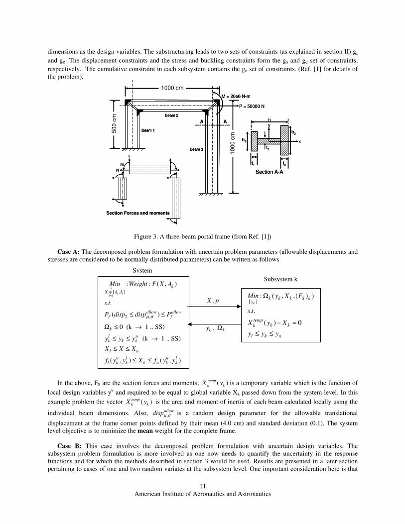
Figure 3. A three-beam portal frame (from Ref. [1])

Case A: The decomposed problem formulation with uncertain problem parameters (allowable displacements and

stresses are considered to be normally distributed parameters) can be written as follows.

In the above, FS are the section forces and moments; ( )tempk kX y is a temporary variable which is the function of

local design variables yk and required to be equal to global variable Xk passed down from the system level. In this

example problem the vector ( )tempk kX y is the area and moment of inertia of each beam calculated locally using the

individual beam dimensions. Also, ,allow

dispµ σ is a random design parameter for the allowable translational

displacement at the frame corner points defined by their mean (4.0 cm) and standard deviation (0.1). The system

level objective is to minimize the mean weight for the complete frame.

Case B: This case involves the decomposed problem formulation with uncertain design variables. The

subsystem problem formulation is more involved as one now needs to quantify the uncertainty in the response

functions and for which the methods described in section 3 would be used. Results are presented in a later section

pertaining to cases of one and two random variates at the subsystem level. One important consideration here is that

ky , kΩ

3

1[ , ]

2 ,

: : ( , )

. .

( )

0 (k 1 .. SS)

(k 1 .. SS)

( , ) ( , )

i ii

k

X A I

allow allowf f

k

l uk k k

l u

u l u ll k k k u k k

Min Weight F X A

s t

P disp disp P

y y y

X X X

f y y X f y y

µ σ

=∈

≤ ≤

Ω ≤ →

≤ ≤ →

≤ ≤

≤ ≤

[ ]: ( , , ( ) )

. .

( ) 0

k

k k k S ky

tempk kk

l k u

Min y X F

s t

X y X

y y y

Ω

− =

≤ ≤

System

Subsystem k

,X p

A A

1000 cm

50

0 c

m

10

00

cm

Beam 1

Beam 2

Beam 3

P = 50000 N

M = 20e6 N-m

N

M

T

Section Forces and moments

y

x

b2

b1

t2t1

t3

Section A-A

hA A

1000 cm

50

0 c

m

10

00

cm

Beam 1

Beam 2

Beam 3

P = 50000 N

M = 20e6 N-m

A A

1000 cm

50

0 c

m

10

00

cm

Beam 1

Beam 2

Beam 3

P = 50000 N

M = 20e6 N-m

N

M

T

N

M

T

Section Forces and moments

y

x

b2

b1

t2t1

t3

Section A-A

h

y

x

b2

b1

t2t1

t3

Section A-A

h


12

at the coordination level the displacements (d) and section forces (FS) in each beam depend on all the six variables

i.e. 1 1 2 2 3 3, ( , , , , , )Sd F f A I A I A I= . The formulation for Case B – 2 for this example is defined below. Here we

assume that the subsystem “k” and “k+1” are those with some of the local design variables being uncertain. The

other subsystems can be solved subsequent to solution of these subsystems.

VI. Numerical results

The deterministic design optimization problem was solved first to establish a baseline for comparison of results

obtained from nondeterministic analysis. Both the all-in-one strategy for design and the decomposition formulation

of the previous sections were solved and the results are presented in Table 1. As can be observed from these results,

there is good agreement between the results from the two approaches. These results also compare well against those

available in the literature for this design problem.

Table – 1 Comparison of All-in-one and decomposition approaches

Beam 1 Beam2 Beam 3 Beam 1 Beam2 Beam3

h1 (cm) 66.0329 42.9694 75.9842 63.8206 42.2073 78.4934

b1(cm) 10 10 10 10 10 10

b2(cm) 10 10 10 10 10 10

t1(cm) 0.6709 0.6796 0.8351 0.6893 0.6938 0.8514

t2(cm) 0.6784 0.6146 0.8459 0.6974 0.6362 0.8624

t3(cm) 0.3744 0.2 0.4725 0.367 0.2 0.4834

92053 93327

Decomposed solutionMin.

Volume

cm3

All-in-one solution

3

1[ , ]

,

: : ( )

. .

( )


( 0) (k 1 .. SS)

( ) (k 1 .. SS)

( )

( , )

i ii

k

X A I

allow allow

f f

th

allow

f k f

l u allow

f k k k f

l u allow

f f

l u l

k k

Min Weight F A

s t

P disp disp P

k k

P P

P y y y P

P X X X P

f y y

µ σ

=∈

≤ ≤

+

Ω ≤ ≤ →

≤ ≤ ≤ →

≤ ≤ ≤

( , )u u l

k k kX f y y≤ ≤

System Level (Portal Frame)

[ ]

1 1

,

2 2

,

3 3

,

: ( , , ( ) )

. .

( )

( )

( )

k

k k k S ky

allow j

f f allow

allow j

f f allow

allow j

f f allow

l u

k

Min y X F

s t

P axialstress axialstress P

P shearstress shearstress P

P bucklingstress stress P

y y y

µ

µ σ

µ σ

µ σ

µ

Ω

≤ ≤

≤ ≤

≤ ≤

≤ ≤

1

1 1 1 1[ ]

1 1

,

2 2

,

3 3

,

1

: ( , , ( ) )

. .

( )

( )

( )

k

k k k S ky

allow j

f f allow

allow j

f f allow

allow j

f f allow

l u

k

Min y X F

s t




y y y

µ

µ σ

µ σ

µ σ

µ

++ + + +

+

Ω

≤ ≤

≤ ≤

≤ ≤

≤ ≤

Subsystem “k”

Subsystem “k+1”

Coupling to accommodate

local variable uncertainties


Subsystem “k+n”

k

k

X

y

∂

∂

1

1

k

k

X

y

+

+

∂

∂

, ( )k S kX F

1 1, ( )k s kX F+ +

3

1[ , ]

,

: : ( )

. .

( )


( 0) (k 1 .. SS)

( ) (k 1 .. SS)

( )

( , )

i ii

k

X A I

allow allow

f f

th

allow

f k f

l u allow

f k k k f

l u allow

f f

l u l

k k

Min Weight F A

s t

P disp disp P

k k

P P

P y y y P

P X X X P

f y y

µ σ

=∈

≤ ≤

+

Ω ≤ ≤ →

≤ ≤ ≤ →

≤ ≤ ≤

( , )u u l

k k kX f y y≤ ≤


3

1[ , ]

,

: : ( )

. .

( )


( 0) (k 1 .. SS)

( ) (k 1 .. SS)

( )

( , )

i ii

k

X A I

allow allow

f f

th

allow

f k f

l u allow

f k k k f

l u allow

f f

l u l

k k

Min Weight F A

s t

P disp disp P

k k

P P

P y y y P

P X X X P

f y y

µ σ

=∈

≤ ≤

+

Ω ≤ ≤ →

≤ ≤ ≤ →

≤ ≤ ≤

( , )u u l

k k kX f y y≤ ≤


[ ]

1 1

,

2 2

,

3 3

,

: ( , , ( ) )

. .

( )

( )

( )

k

k k k S ky

allow j

f f allow

allow j

f f allow

allow j

f f allow

l u

k

Min y X F

s t




y y y

µ

µ σ

µ σ

µ σ

µ

Ω

≤ ≤

≤ ≤

≤ ≤

≤ ≤

1

1 1 1 1[ ]

1 1

,

2 2

,

3 3

,

1

: ( , , ( ) )

. .

( )

( )

( )

k

k k k S ky

allow j

f f allow

allow j

f f allow

allow j

f f allow

l u

k

Min y X F

s t




y y y

µ

µ σ

µ σ

µ σ

µ

++ + + +

+

Ω

≤ ≤

≤ ≤

≤ ≤

≤ ≤

Subsystem “k”

Subsystem “k+1”

Coupling to accommodate

local variable uncertainties


Subsystem “k+n”

k

k

X

y

∂

∂

1

1

k

k

X

y

+

+

∂

∂

, ( )k S kX F

1 1, ( )k s kX F+ +


13

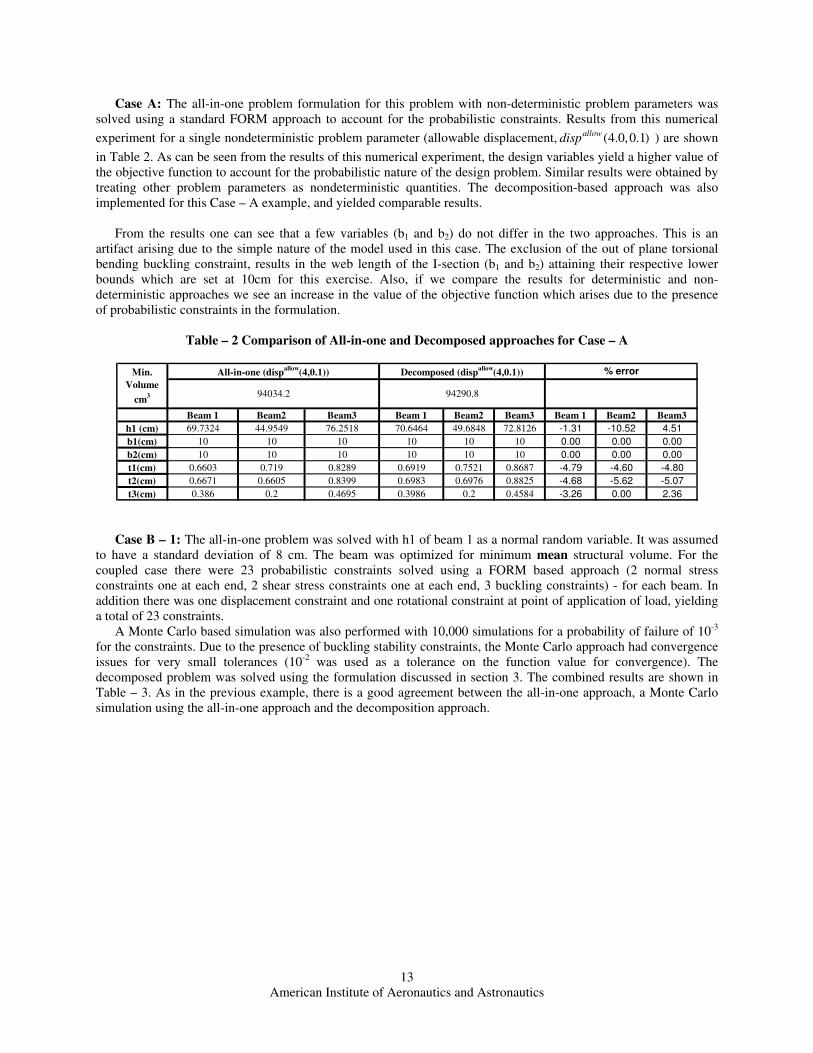
Case A: The all-in-one problem formulation for this problem with non-deterministic problem parameters was

solved using a standard FORM approach to account for the probabilistic constraints. Results from this numerical

experiment for a single nondeterministic problem parameter (allowable displacement, (4.0,0.1)allowdisp ) are shown

in Table 2. As can be seen from the results of this numerical experiment, the design variables yield a higher value of

the objective function to account for the probabilistic nature of the design problem. Similar results were obtained by

treating other problem parameters as nondeterministic quantities. The decomposition-based approach was also

implemented for this Case – A example, and yielded comparable results.

From the results one can see that a few variables (b1 and b2) do not differ in the two approaches. This is an

artifact arising due to the simple nature of the model used in this case. The exclusion of the out of plane torsional

bending buckling constraint, results in the web length of the I-section (b1 and b2) attaining their respective lower

bounds which are set at 10cm for this exercise. Also, if we compare the results for deterministic and non-

deterministic approaches we see an increase in the value of the objective function which arises due to the presence

of probabilistic constraints in the formulation.

Table – 2 Comparison of All-in-one and Decomposed approaches for Case – A

Beam 1 Beam2 Beam3 Beam 1 Beam2 Beam3 Beam 1 Beam2 Beam3

h1 (cm) 69.7324 44.9549 76.2518 70.6464 49.6848 72.8126 -1.31 -10.52 4.51

b1(cm) 10 10 10 10 10 10 0.00 0.00 0.00

b2(cm) 10 10 10 10 10 10 0.00 0.00 0.00

t1(cm) 0.6603 0.719 0.8289 0.6919 0.7521 0.8687 -4.79 -4.60 -4.80

t2(cm) 0.6671 0.6605 0.8399 0.6983 0.6976 0.8825 -4.68 -5.62 -5.07

t3(cm) 0.386 0.2 0.4695 0.3986 0.2 0.4584 -3.26 0.00 2.36

94290.894034.2

% errorDecomposed (dispallow

(4,0.1))Min.

Volume

cm3

All-in-one (dispallow

(4,0.1))

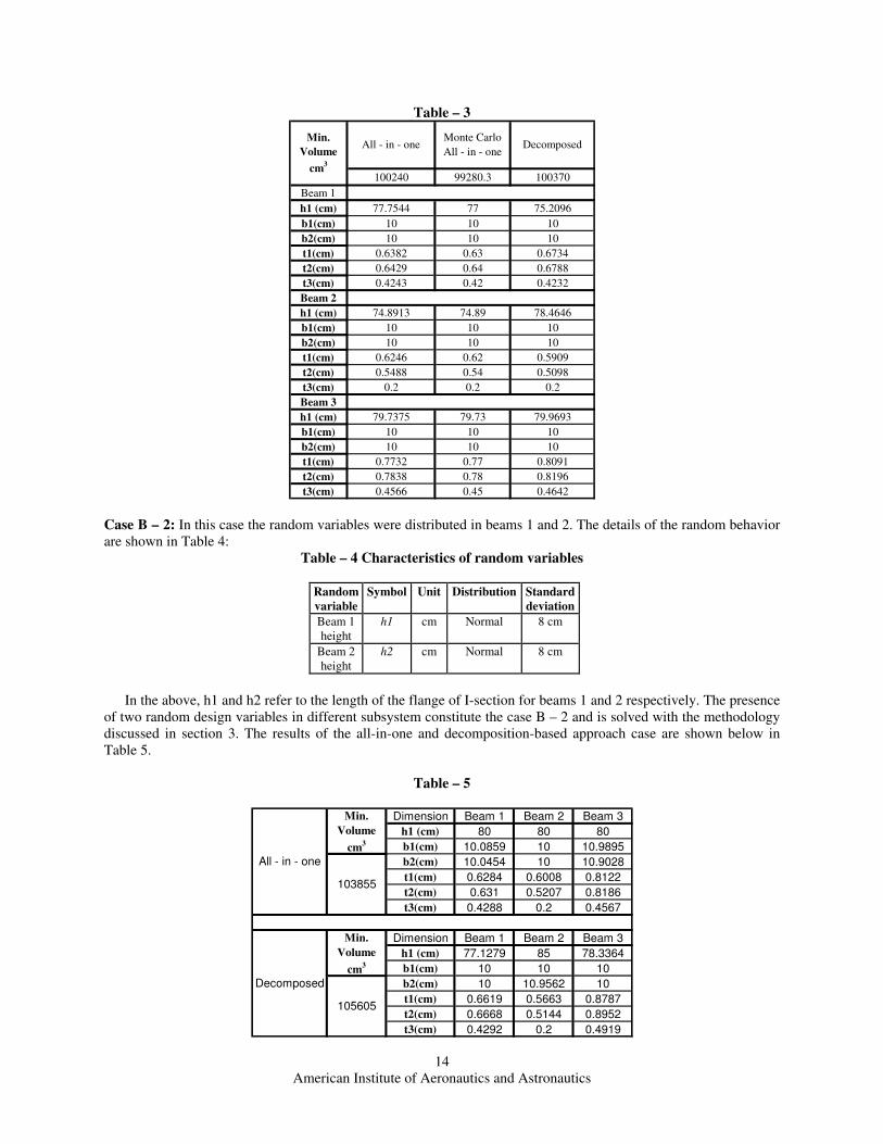
Case B – 1: The all-in-one problem was solved with h1 of beam 1 as a normal random variable. It was assumed

to have a standard deviation of 8 cm. The beam was optimized for minimum mean structural volume. For the

coupled case there were 23 probabilistic constraints solved using a FORM based approach (2 normal stress

constraints one at each end, 2 shear stress constraints one at each end, 3 buckling constraints) - for each beam. In

addition there was one displacement constraint and one rotational constraint at point of application of load, yielding

a total of 23 constraints.

A Monte Carlo based simulation was also performed with 10,000 simulations for a probability of failure of 10-3

for the constraints. Due to the presence of buckling stability constraints, the Monte Carlo approach had convergence

issues for very small tolerances (10-2 was used as a tolerance on the function value for convergence). The

decomposed problem was solved using the formulation discussed in section 3. The combined results are shown in

Table – 3. As in the previous example, there is a good agreement between the all-in-one approach, a Monte Carlo

simulation using the all-in-one approach and the decomposition approach.


14

Table – 3

100240 99280.3 100370

Beam 1

h1 (cm) 77.7544 77 75.2096

b1(cm) 10 10 10

b2(cm) 10 10 10

t1(cm) 0.6382 0.63 0.6734

t2(cm) 0.6429 0.64 0.6788

t3(cm) 0.4243 0.42 0.4232

Beam 2

h1 (cm) 74.8913 74.89 78.4646

b1(cm) 10 10 10

b2(cm) 10 10 10

t1(cm) 0.6246 0.62 0.5909

t2(cm) 0.5488 0.54 0.5098

t3(cm) 0.2 0.2 0.2

Beam 3

h1 (cm) 79.7375 79.73 79.9693

b1(cm) 10 10 10

b2(cm) 10 10 10

t1(cm) 0.7732 0.77 0.8091

t2(cm) 0.7838 0.78 0.8196

t3(cm) 0.4566 0.45 0.4642

Min.

Volume

cm3

All - in - oneMonte Carlo

All - in - oneDecomposed

Case B – 2: In this case the random variables were distributed in beams 1 and 2. The details of the random behavior

are shown in Table 4:

Table – 4 Characteristics of random variables

Random

variable

Symbol Unit Distribution Standard

deviation

Beam 1

height

h1 cm Normal 8 cm

Beam 2

height

h2 cm Normal 8 cm

In the above, h1 and h2 refer to the length of the flange of I-section for beams 1 and 2 respectively. The presence

of two random design variables in different subsystem constitute the case B – 2 and is solved with the methodology

discussed in section 3. The results of the all-in-one and decomposition-based approach case are shown below in

Table 5.

Table – 5

Dimension Beam 1 Beam 2 Beam 3

h1 (cm) 80 80 80

b1(cm) 10.0859 10 10.9895

b2(cm) 10.0454 10 10.9028

t1(cm) 0.6284 0.6008 0.8122

t2(cm) 0.631 0.5207 0.8186

t3(cm) 0.4288 0.2 0.4567


h1 (cm) 77.1279 85 78.3364

b1(cm) 10 10 10

b2(cm) 10 10.9562 10

t1(cm) 0.6619 0.5663 0.8787

t2(cm) 0.6668 0.5144 0.8952

t3(cm) 0.4292 0.2 0.4919

All - in - one

Decomposed

Min.

Volume

cm3

Min.

Volume

cm3

105605

103855


15

The optimal results obtained in each of the cases, for all-in-one approach and the decomposition based approach,

show good agreement with each other. The deterministic design optimization results presented shown in Table 1

demonstrates the effectiveness of the decomposition based design procedure. From the results we can see that, as

before variables b1 and b2 do not differ for the two approaches. This is due to the exclusion of the out of plane

torsional bending buckling constraint. In the absence of this constraint the depth-to-flange ratio is unusually large for

the I-section, as the flange lengths then go to their lower bounds (10cm in our case). This however has no bearing on

the numerical verification of the method.

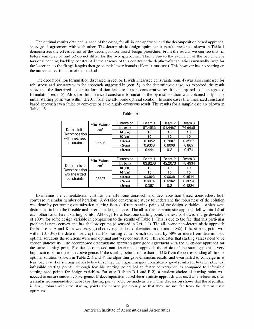
The decomposition formulation discussed in section II with linearized constraints (eqn. 4) was also compared for

robustness and accuracy with the approach suggested in (eqn. 5) in the deterministic case. As expected, the result

show that the linearized constraint formulation leads to a more conservative result as compared to the suggested

formulation (eqn. 5). Also, for the linearized constraint formulation the optimal solution was obtained only if the

initial starting point was within ± 20% from the all-in-one optimal solution. In some cases the, linearized constraint

based approach even failed to converge or gave highly erroneous result. The results for a sample case are shown in

Table – 6.

Table – 6


h1 (cm) 57.4533 51.4487 76.6685

b1(cm) 10 10 10

b2(cm) 10 10 10

t1(cm) 0.9052 0.7007 0.8537

t2(cm) 0.9338 0.6096 0.865

t3(cm) 0.444 0.2 0.474


h1 (cm) 63.8206 42.2073 78.4934

b1(cm) 10 10 10

b2(cm) 10 10 10

t1(cm) 0.6893 0.6938 0.8514

t2(cm) 0.6974 0.6362 0.8624

t3(cm) 0.367 0.2 0.4834

Determinitic

Decomposition

with linearized

constraints

Min. Volume

cm3

96596

Deterministic

Decomposition

w/o linearized

constraints

Min. Volume

cm3

93327

Examining the computational cost for the all-in-one approach and decomposition based approaches; both

converge in similar number of iterations. A detailed convergence study to understand the robustness of the solution

was done by performing optimization starting from different starting points of the design variables – which were

distributed in both the feasible and infeasible design space. The all-in-one deterministic approach fell within 1% of

each other for different starting points. Although for at least one starting point, the results showed a large deviation

of 100% for some design variable in comparison to the results of Table 1. This is due to the fact that this particular

problem is non- convex and has shallow optima (discussed in Ref. [1]). The all-in-one non-deterministic approach

for both case A and B showed very good convergence (max. deviation in optima of 8%) if the starting point was

within ( ± 30%) the deterministic optima. For starting values which deviated by 50% or more from deterministic

optimal solutions the solutions were non optimal and very conservative. This indicates that starting values need to be

chosen judiciously. The decomposed deterministic approach gave good agreement with the all-in-one approach for

the same starting point. For the decomposed non deterministic approach the choice of the starting point is very

important to ensure smooth convergence. If the starting point is more than ± 15% from the corresponding all-in-one

optimal solution (shown in Table 2, 3 and 4) the algorithm gave erroneous results and even failed to converge in at

least one case. For starting values below this range the algorithm gave consistently good results for both feasible and

infeasible starting points, although feasible starting points led to faster convergence as compared to infeasible

starting seed points for design variables. For case-B (both B-1 and B-2), a prudent choice of starting point was

needed to ensure smooth convergence. If decomposition based deterministic approach was used as a reference, then

a similar recommendation about the starting points could be made as well. This discussion shows that the algorithm

is fairly robust when the starting points are chosen judiciously so that they are not far from the deterministic

optimum.


16

Another interesting aspect of the uncertainty propagation in a decomposed scenario is the fact that the designer

can filter and restrict the system level randomness to either a single or multiple subsystems of choice. To understand

this with an example, consider a predefined randomness for the area of cross section and the moment of inertia of

the I-section beam 1. Due to the decomposed nature of the optimization problem the designer can decide where to

confine this randomness both in terms of which subsystem(s) and furthermore, to which exact subset of design

variables inside a subsystem. This novel approach to manage uncertainty in system right at the design optimization

process can prove to be a handy tool as it gives the designer a way to distribute the randomness in subsystem of their

choice. Apart from this, the designer can also restrict the influence of a subsystem level uncertainty on the system

level performance by concentrating the uncertainty in less critical subsystem.

Closing Remarks

The paper develops a formal decomposition-based design approach in the presence of nondeterministic problem

parameters and design variables. The scope of the problem is limited to case where hierarchical partitioning is

possible and where there is top-down or bottom-up flow of information between the decoupled levels. The focus of

the work resides in looking at how uncertainties propagate in such coupled problems, how design problem

formulations can be proposed to account for uncertainty propagation, and what computationally expedient tools can

be used to improve numerical efficiency and robustness of the design problem. The primary focus of this

development was presented in the context of a simple two-level structural design problem. An extension of this

approach to the analysis and design of multiscale composite structural systems for damage tolerance is currently

being pursued and will be reported in a different publication.

Acknowledgement

The support received for this work under a grant from the AFOSR (Award no: FA 9550-05-1-0140) is gratefully

acknowledged.

References:

1. J. Sobieszczanski-Sobieski, B. James and A. Dovi. Structural Optimization by multilevel decomposition. In

AIAA Journal, Vol. 23, No.11, Nov. 1985.

2. J. Sobieszczanski-Sobieski. Optimization by decomposition: A step from hierarchic to non-hierarchic

systems. In Second NASA/Air Force Symposium on Recent Advances in Multidisciplinary Analysis and

Optimization, 1998. NASA Conference Publication 3031, Part1.

3. I. Kroo, S. Altus, R. Braun, P. Gage and J. Sobieski. Multidisciplinary optimization methods for aircraft

preliminary design. In Proceedings of the 5th

AIAA/NASA/USAF/ISSMO Symposium on Multidisciplinary

Analysis and Optimization, pages 697-707, 1994. Paper No. AIAA-94-4325-CP.

4. R.J. Balling and J. Sobieszczanski-Sobieski. “Optimization of coupled systems: A critical overview”. In

Proceedings of the 5th AIAA/USAF/NASA/ISSMO Symposium on Multidisciplinary Analysis and

Optimization, pages 753–773, Panama City, Florida, 1994.

5. J. Sobieszczanski-Sobieski and R.T. Haftka. “Multidisciplinary aerospace design optimization survey of

recent developments”. In Structural Optimization, 14(1):1–23, 1997.

6. D. Padmanabhan and S. Batill. Decomposition strategies for reliability based optimization in

multidisciplinary system design. In Proceedings of the 95th

AIAA/NASA/USAF/ISSMO Symposium on

Multidisciplinary Analysis and Optimization, 2002. Paper No. AIAA 2002-5471.


17

7. Kokkolaras, M., Mourelatos, Z. P., and Papalambros, P. Y. Design Optimization of Hierarchically

Decomposed Multilevel System under Uncertainty". Journal of Mechanical Design, Vol. 128, No. 2, 2006,

503-508.

8. R. Khire, P. Hajela, and Yehia Bahei-El Din. Handling Uncertainty Propagation in Laminated Composites

Through Multiscale Modeling of Progressive Failure. In Proceedings of the 48th AIAA/ASME/ASCE/AHS

SDM Conference, April 22-25, 2007, Honolulu, Hawaii.

9. R.H. Sues and M.A. Cesare. “An innovative framework for reliability-based MDO”. In Proceedings of the

41th AIAA/ASME/ASCE/AHS/ASC Structures, Structural Dynamics, and Materials Conference, Atlanta,

Georgia, 2000.

10. R.H. Sues, M.A. Cesare, S.S. Pageau, and Y.T. Wu. “Reliability-based optimization considering

manufacturing and operational uncertainties”. Journal of Aerospace Engineering, 14:166–174, 2001.

11. X. Gu, J.E. Renaud, L.M. Ashe, S.M. Batill, A.S. Budhiraja, and L.J. Krajewski. “Decision-based

collaborative optimization under uncertainty”. In Proceedings of the 27th

ASME Design Automation

Conference, Baltimore, Maryland, 2001. Paper no. DETC2000/DAC-14297.

12. X. Du andW. Chen. “Methodology for managing the effect of uncertainty in simulation-based systems

design”. AIAA Journal, 38(8):1471–1478, 2000.

13. X. Gu and J.E. Renaud. “Implicit uncertainty propagation for robust collaborative optimization”. In

Proceedings of the 27th ASME Design Automation Conference, Pittsburgh, Pennsylvania, 2001. Paper no.

DETC2001/DAC-21118.

14. X. Gu and J.E. Renaud. “Implementation study of implicit uncertainty propagation in decomposition-based

optimization”. In Proceedings of the 9th AIAA/USAF/NASA/ISSMO Sumposium on Multidisciplinary

Analysis and Optimization, Atlanta, Georgia, 2002. Paper no. AIAA-2002-5416.

15. X. Du and W. Chen. “Efficient uncertainty analysis methods for multidisciplinary robust design”. AIAA

Journal, 40(3):545–552, 2002.

16. G. Kresselmier and G. Steinhauser. Systematic control design by optimizing a vector performance index. In

Proceedings of IEAC Symposium on Computer Aided Design of Control Systems, pages 113-117, Zurich,

1971.

17. J. Sobieszczanski-Sobieski, J. Barthelemy and K.M. Riley. Sensitivity of optimum solutions to problem

parameters. In AIAA Journal, Vol 20, Sept. 1982, page 1291.

18. G.N. Vanderplaats, Numerical Optimization Techniques for Engineering design, Vanderplaats Research &

Development, Inc. 2004

19. P. Hajela, L. Berke. Neural Network based decomposition on optimal structural synthesis. In International

Journal of Computing Systems in Engineering. Vol. 2, No. 5/6, 1991.

20. A. Haldar and S. Mahadevan. Probability, Reliability and Statistical Methods in Engineering Design. John

Wiley, 2000.

21. S.-K. Choi, R.V. Grandhi, R. A. Cranfield. Reliability-based Structural Design. Springer, 2006.

22. S. Rahman, and H. Xu. A Univariate Dimension-Reduction Method for Multi-dimensional Integration in

Stochastic Mechanics. Probabilistic Engineering Mechanics, Vol. 19, pp. 393-408, 2004.

Date post:	10-Dec-2016
Category:	Documents
Upload:	prabhat
View:	213 times
Download:	1 times

[American Institute of Aeronautics and Astronautics 49th AIAA/ASME/ASCE/AHS/ASC Structures,...

Documents