Direct Quadrature Method of Moments Solution of the
Fokker-Planck Equation for Stochastic Processes in
Aeroelasticity
Peter J. Attar∗ and Prakash Vedula †
The University of Oklahoma
The direct quadrature method of moments (DQMOM) is presented as an efficient andaccurate means of numerically computing solutions of the Fokker-Planck equation. Thetheoretical details of the solution procedure are first presented. The method is then usedto solve Fokker-Planck equations for both one-dimensional and two-dimensional (noisy vander Pol oscillator and saddle node/subcritical Hopf bifurcation example) processes whichpossess nonlinear stochastic differential equations. Higher order moments of the station-ary solutions are computed and prove to be very accurate when compared to analytic (1Dprocess) and Monte-Carlo (2D process) solutions. Trends in the standard deviation andcoefficient of kurtosis with respect to additive noise level and bifurcation parameter arereported for what appears to be the first time for the saddle-node/subcritical Hopf bifu-cation problem. The deterministic form of this problem exhibits hysteresis which is oftena phenomenon present in more complex nonlinear aeroelastic sytems. Finally statisticalresults are shown for a typical section airfoil with nonlinear stiffness subjected to randomloading. The constants for the nonlinear stiffness are chosen such that the deterministicbehavior exhibits both a saddle node and subcritcal bifurcation. Standard deviation re-sults computed using DQMOM for a reduced frequency below the deterministic saddlenode bifurcation point compare well with Monte-Carlo results.
Nomenclature
′ ddτ
α pitch degree of freedomωh plunge uncoupled natural frequencyωα pitch uncoupled natural frequencyh normalized plunge degree of freedom h/bτ nondimensional time, τ = tωα
ξh plunge mode damping ratioξα pitch mode damping ratiob reference airfoil lengthe distance from aerodynamic center to elastic axisk reduced frequency ωαb
UKh constant for linear plunge stiffness termKnl
h constant for cubic plunge stiffness termKα constant for linear pitch stiffness termKnl1
α constant for cubic pitch stiffness termKnl2
α constant for quintic pitch stiffness termm airfoil mass per unit lengthrα radius of gyrationSα mass unbalance
∗Assistant Professor, Department of Aerospace and Mechanical Engineering, Member AIAA, e-mail:[email protected].†Assistant Professor, Department of Aerospace and Mechanical Engineering Engineering, e-mail:[email protected]
1 of 28
American Institute of Aeronautics and Astronautics
49th AIAA/ASME/ASCE/AHS/ASC Structures, Structural Dynamics, and Materials Conference <br> 16t7 - 10 April 2008, Schaumburg, IL
Characterization of the response of stochastic systems is of interest for engineers in many different disci-plines. This is particularly true in the field of structural dynamics where loads and various system parameterscan often be thought of as random processes. For example in the field of aeroelasticity, Ibrahim and hiscolleagues considered the pressure fluctuations due to a turbulent boundary layer as random forces whenanalyzing panel flutter.1–3 Vaicaitis et al.4 and Olson5 also considered this problem and utilized MonteCarlo simulations. Recently much work has been done in the area of parametric uncertainty quantificationfor aeroelastic problems. For a nice overview of some of this work and remaining challenges see the work ofPettit.6
The response of a structural dynamic system to random excitation having delta-correlation can be con-sidered a Markov process. Furthermore even if a process is non-Markovian, through the introduction ofadditional random variables, one can get a Markov process.7 The transition probability density for a Markovprocess is governed by an appropriate Fokker-Planck (FP) equation. Exact solutions of the FP equation areknown for only a few systems. In most cases, approximate solutions need to be found using either analytic ornumerical methods. The text by Risken7 presents many such analytical methods. Examples of approximateanalytical solutions are the van Kampen expansion method,8, 9 the method of matrix continued fractions10
and path integral solutions.11 In terms of numerical methods, finite difference and finite element methodsappear to be the most popular.12–15 While these methods can give accurate solutions, the computationalexpense can be prohibitive for Fokker-Planck equations with dimensions larger than two.
In this paper we present an efficient and accurate method for the solution of the Fokker-Planck equationsfor stochastic processes. This method is based upon the direct quadrature method of moments (DQMOM)first introduced by Fox and colleagues16–18 for the numerical solution of the population balance equations formulti-phase flow predictions. Recently this method has also been used to compute numerical solutions forthe Boltzmann equation by the second author19 and has been used for one-dimensional and two-dimensionalFokker-Planck equations arising in nonlinear dynamics.20 Here we will show additional results for a two-dimensional Fokker-Planck equation which corresponds to a deterministic system which has both a saddlenode bifurcation and a subcritical Hopf bifurcation. Knowledge of the statistical moment behavior of sucha system is important due to its similarity to more complex nonlinear aeroelastic systems. Finally resultswill be presented for such an aeroelastic system, a typical section airfoil with 2 degrees of freedom (pitchand plunge). A nonlinear structure model in the form of nonlinear springs in the pitch and plunge degreesof freedom is presented for this model. This dynamical system results in a four-dimensional Fokker-Planckequation.
II. Theory
Given the set of stochastic differential equations in N variables x = {x1,x2,....xN}:
xi = hi(x, t) + gij(x, t)Γj(t), (1)
where the Γj(t) are Gaussian random variables with the following correlations:
< Γi(t) > = 0 < Γi(t)Γj(t′) >= 2δijδ(t − t′), (2)
with δij the Kronecker delta and δ(t − t′) the delta function, a Fokker-Planck equation for the transitionprobability P (x, t|x′, t′) can be written in the following form:
∂P (x, t|x′, t′)
∂t= − ∂
∂xi[D
(1)i (x, t)P (x, t|x′, t′)]+ (3)
∂2
∂xi∂xj[D
(2)ij (x, t)P (x, t|x′, t′)].
2 of 28
American Institute of Aeronautics and Astronautics
It can also be shown that the probability density function f(x, t) also satisfies the Fokker-Planck equation:
∂f(x, t)
∂t= − ∂
∂xi[D
(1)i (x, t)f(x, t)] +
∂2
∂xi∂xj[D
(2)ij (x, t)f(x, t)]. (4)
In Eq. 3 and 4 the drift (D(1)i (x, t)) and diffusion (D
(2)ij (x, t)) coefficients are defined as (using the notation
of Eq. 1):
D(1)i (x, t) = hi(x, t) (5)
D(2)ij (x, t) = gik(x, t)gjk(x, t) (6)
and are derived using the Ito calculus.7 Note in Eqs. 3 and 4 summation notation is assumed.In order to simplify the derivations, Eq. 4 will be specialized to the problem of N=2 and all cross diffusion
terms will be assumed to be zero(D(2)12 = D
(2)21 = 0). Also D
(2)11 will be assumed to be zero. In practice,
generalizing the method (to be discussed in this paper) to higher dimensions with all terms included doesnot complicate the computational procedure. With the above simplifications we get the following for theFokker-Planck equations:
∂f(x, t)
∂t= − ∂
∂x[D
(1)1 f(x, t)] − ∂
∂y[D
(1)2 f(x, t)]+ (7)
+∂2
∂y2(D
(2)22 f(x, t)) ,
where now x = {x, y}T .In the direct quadrature method of moments approach the probabilty density is written as a weighted
summation of products of Dirac delta functions:
f(x, t) =
M∑
i=1
wi(t)δ(x − xi(t))δ(y − yi(t)) , (8)
where M is the number of delta functions (compute nodes) and wi(t), xi(t) and yi(t) are the dependentvariables for compute node i. In the rest of the paper the wi will be called weights and xi, yi the abscissas.Also the explicit expression of the dependent variables as functions of time will be dropped in order to
condense the notation. If the delta functions δ(x−xi) and δ(y− yi) are written as δ(x)i and δ
(y)i respectively,
substitution of Eq. 8 into Eq. 7 results in the following:
M∑
i=1
[
∂wi
∂tδ(x)i δ
(y)i − wi
∂xi
∂t
∂δ(x)i
∂xδ(y)i − wi
∂yi
∂tδ(x)i
∂δ(y)i
∂y
]
=
M∑
i=1
[
− ∂
∂x(D
(1)1 wiδ
(x)i δ
(y)i )
− ∂
∂y(D
(1)2 wiδ
(x)i δ
(y)i ) +
∂2
∂y2(D
(2)22 wiδ
(x)i δ
(y)i )
]
. (9)
Defining new variables, which we will call the weighted abscissas, µ(x)i = wixi and µ
(y)i = wiyi, Eq. 9 becomes:
M∑
i=1
[
∂wi
∂tδ(x)i δ
(y)i − xi
∂µ(x)i
∂t
∂δ(x)i
∂xδ(y)i + xi
∂wi
∂t
∂δ(x)i
∂xδ(y)i − ∂µ
(y)i
∂t
∂δ(y)i
∂yδ(x)i + (10)
yi∂wi
∂t
∂δ(y)i
∂yδ(x)i
]
=
M∑
i=1
[
− ∂
∂x(D
(1)1 wiδ
(x)i δ
(y)i ) − ∂
∂y(D
(1)2 wiδ
(x)i δ
(y)i )+
+∂2
∂y2(D
(2)22 wiδ
(x)i δ
(y)i )
]
.
At this point we have one equation in 3M unknowns. In order to close this equation, we will take 3Mmoments of it. Recalling that the generalized moment < xrys >, for non-negative integers r and s, is givenby the expression:
< xrys >=
∫
∞
−∞
xrysf(x, y, t) dxdy, (11)
3 of 28
American Institute of Aeronautics and Astronautics
the evolution of < xrys > can be obtained by taking the moment of Eq. 10 (after interchanging the order ofsummation and integration and combining the sums on the left and right hand sides):
M∑
i=1
[
∫
∞
−∞
∫
∞
−∞
xrys
[
∂wi
∂tδ(x)i δ
(y)i − xi
∂µ(x)i
∂t
∂δ(x)i
∂xδ(y)i + xi
∂wi
∂t
∂δ(x)i
∂xδ(y)i − (12)
∂µ(y)i
∂t
∂δ(y)i
∂yδ(x)i + yi
∂wi
∂t
∂δ(y)i
∂yδ(x)i = − ∂
∂x(D
(1)1 wiδ
(x)i δ
(y)i )
− ∂
∂y(D
(1)2 wiδ
(x)i δ
(y)i ) +
∂2
∂y2(D
(2)22 wiδ
(x)i δ
(y)i )
]
dxdy
]
.
In simplifying Eq. 12 the following properties of the Dirac delta function are used:
∫
xrδ(x − xi)dx = xri (13)
∫
xr dδ(x − xi)
dxdx = −rxr−1
i . (14)
So on using Eq. 13 and 14 and integrating by parts the right hand side of Eq. 12 we get the followingequation:
M∑
i=1
[
xri y
si
∂wi
∂t+ rxr−1
i ysi
∂µ(x)i
∂t− rxr−1
i ysi xi
∂wi
∂t+ sxr
i ys−1i
∂µ(y)i
∂t(15)
−sxri y
s−1i yi
∂wi
∂t= −xrysD
(1)1 wiδ
(x)i δ
(y)i |∞
−∞+ rxr−1
i ysi D
(1)1 |xi,yi
wi−
xrysD(1)2 wiδ
(x)i δ
(y)i |∞
−∞+ sxr
i ys−1i D
(1)2 |xi,yi
wi + xrys ∂
∂y
(
D(2)22 wiδ
(x)i δ
(y)i
)
|∞−∞
−
sxrys−1D(2)22 wiδ
(x)i δ
(y)i |∞
−∞+ s(s − 1)xr
i ys−2i D
(2)22 |xi,yi
]
,
where |xi,yidenotes evaluation of the drift and diffusion terms at x = xi and y = yi. Using the property that
the probability density vanishes at positive and negative infinity and the assumption of a smooth probabilitydensity function (hence a vanishing derivative of the probability density at positive and negative infinity),the boundary terms in Eq. 15 vanish, leaving after simplification, the following equation:
M∑
i=1
[
[1 − (r + s)]xri y
si
dwi
dt+ rxr−1
i ysi
dµ(1)i
dt+ sxr
i ys−1i
dµ(2)i
dt= (16)
rxr−1i ys
i D(1)1 |xi,yi
wi + sxri y
s−1i D
(1)2 |xi,yi
wi + s(s − 1)xri y
s−2i D
(2)22 |xi,yi
wi
]
This is now a nonlinear differential equation for each of the weights and weighted abscissas. There are 3Msuch equations, which in matrix form can be written as:
Az = F(w,x,y) (17)
where the matrix A is a nonlinear function of the abscissas and z = { dwdt , dµ
(1)
dt , dµ(2)
dt }T . Also w,x,y, andµ are the vectors of weights, abscissas and weighted abscissas respectively. Equation 17 is a set of implicitnonlinear ordinary differential equations. In order solve these equations, the DDASPK software package21–23
is used.
III. Example Problems
Four example problems will be given in this paper to demonstrate the effectiveness of the DQMOMmethod in solving the Fokker-Planck equation. The problems will be presented in order of increasing diffulty.
4 of 28
American Institute of Aeronautics and Astronautics
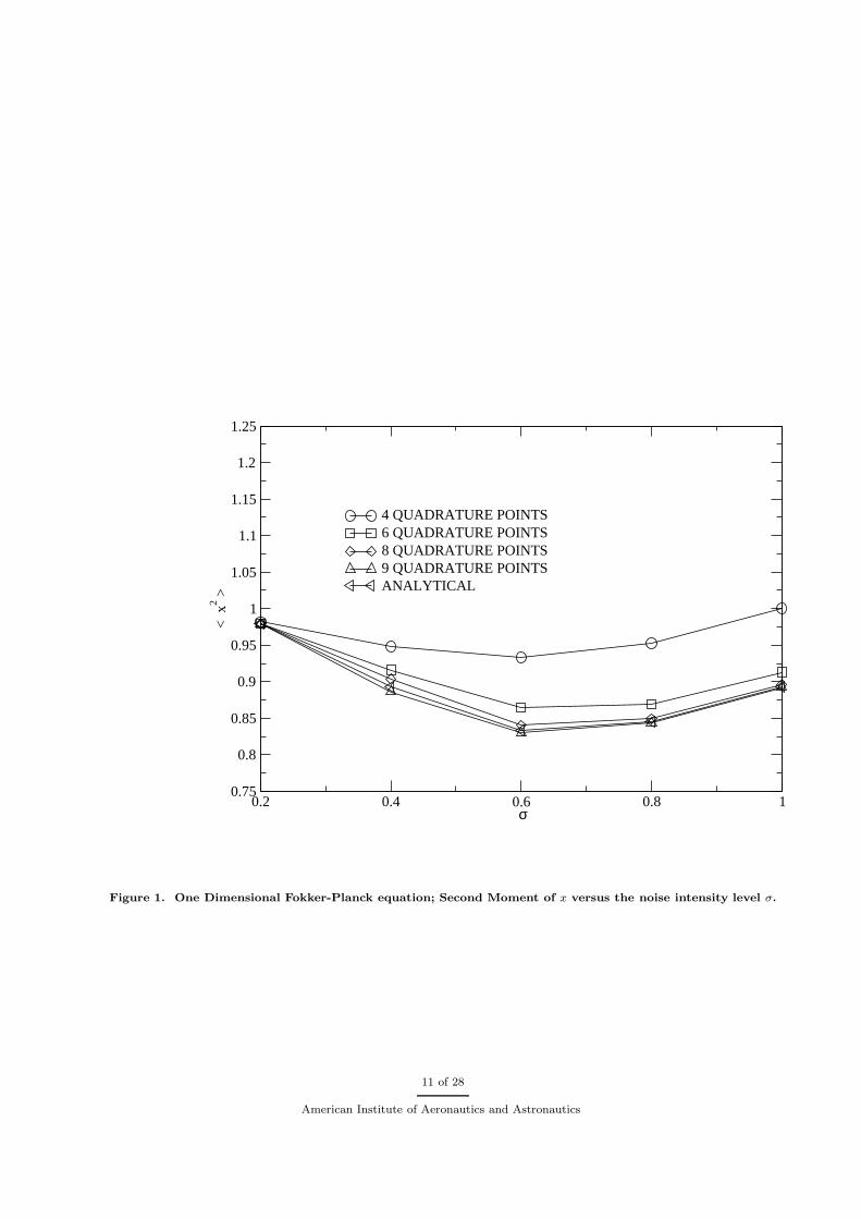
A. 1D Nonlinear Process
The first problem is the nonlinear process with a stochastic ordinary differential equation given by:
dX = (X − X3)dt + σdW , (18)
which has the Fokker-Planck equation given by:
∂f
∂t= − ∂
∂x[(x − x3)f ] +
σ2
2
∂2f
∂x2. (19)
The deterministic counterpart to this equation (dx/dt = x − x3) has two asymptotically stable equilibriumpoints x = ±1 separated by an unstable equilibrium point at x = 0. An analytical solution to Eq. (19) isnot known but the stationary solution is given by
P (x) = ce(x2−0.5x4)/σ2
, (20)
where c is a normalization constant. Figures 1- 3 show the second,fourth and sixth moments as computedby the DQMOM numerical method as a function of the noise level σ. Also shown on these figures arethe analytical results computed via Eq. (20). With only 8 quadrature nodes the DQMOM and analyticalsolutions agree quite well for each of the moments. Also note that all odd moments are zero for this problemand the DQMOM method computes these correctly as well.
B. 2D van der Pol Oscillator
The second problem which is investigated is the van der Pol oscillator subjected to stationary Gaussian whitenoise. If the vector process Z(t) = {x(t), y(t)}T is introduced, where y(t) = x(t), the Ito-type stochasticdifferential equation can be written as:
dZ(t) = f(Z(t))dt + QdW (t). (21)
Here we have
f(Z(t)) =
{
y(t)
−µ[x(t)2 − 1]y(t) − x(t)
}
(22)
Q =
{
0√2D
}
(23)
The corresponding Fokker-Planck equation for this problem can be written as:
∂f
∂t= µ(x2 − 1)f − y
∂f
∂x+ [µ(x2 − 1)y + x]
∂f
∂y+ D
∂2f
∂y2(24)
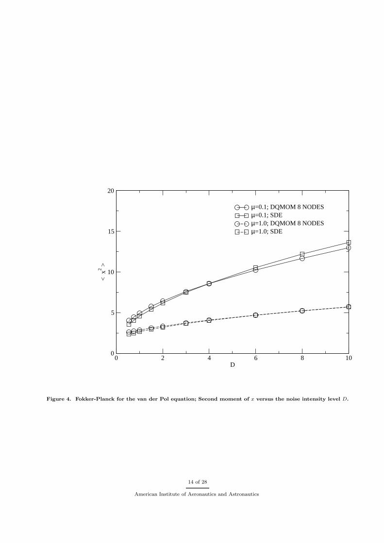
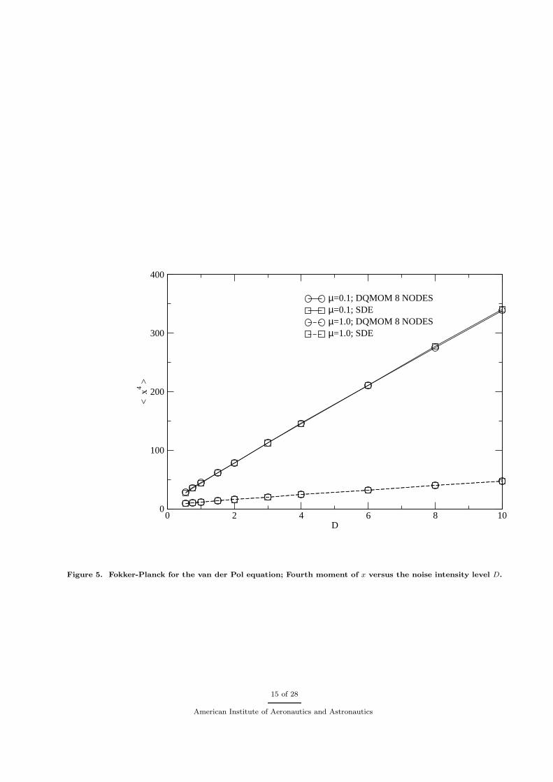
which is solved numerically using the direct quadrature method of moments. The second and fourth momentsof x as computed by a direct quadrature method of moments solution of Eq. (24) is shown in Figs. 4 and 5 forµ = 0.1 and µ = 1.0. Also shown in these figures is a numerical solution of the stochastic differential equation,Eq. (21), using a forward Euler-Maruyama time integration scheme. Due to its simplicity, we restricted ourattention to the commonly used Euler-Maruyama scheme for integration of stochastic differential equations.It is plausible that high-order integration schemes for stochastic differential equations could lead to moreaccurate solutions, with greater computational efficiency. The statistics from this solution were computedusing a Monte Carlo solution with 5×10⁵ particles and a timestep of 0.0005 seconds. These figures also includemoments computed using the stationary solutions from the analytic statistical non-linearization procedurepresented in Ref. 24.In these figures one can see that the second and fourth order moments computed usingan 8 node direct quadrature method of moments solution compare favorably with the direct solution of thestochastic differential equation. Agreement with the statistical non-linearization result is better for smallervalues of the noise level D and the damping parameter µ which is consistent with the approximations madein the analytic method. Note, in order to compute the direct quadrature method of moments solution, allmoments up to fifth order and (r, s) = (6, 0), (5, 1), (4, 2) were taken (see Eq. (12)). The direct quadraturemethod of moments solution is substantially faster than the direct solution of the stochastic differentialequation. On a Intel T2500 2GHz processor 10 seconds of simulation time took 4 seconds of computationaltime using the direct quadrature method of moments solution and 1500 seconds of computational time usingthe Monte Carlo solution of the stochastic differential
5 of 28
American Institute of Aeronautics and Astronautics
C. 2D Nonlinear Process with Saddle Node and Subcritical Bifurcation
The third problem which we will study is a stochastic version of the following nonlinear dynamical systemin cylindrical coordinates:25
r = µr + r3 − r5
θ = ω + br2 (25)
Here ω controls the frequency of infinitesimal oscillations and b determines the nonlinear dependency ofthe frequency on the oscillation amplitude. For −1/4 < µ < 0 there are two attractors. One is a stablelarge amplitude limit cycle oscillation (LCO) and the other is a stable attractor at the origin. At µ = −1/4the large amplitude LCO is destroyed via a saddle-node bifurcation and the only stable attractor is theorigin. At µ = 0 the system undergoes a subcritical Hopf bifurcation and the only attractor left is the largeamplitude limit cycle. This system exhibits a hysteretic behavior which is common in nonlinear aeroelasticsystems26 and presents a dangerous scenario which is often referred to as explosive flutter or “bad LCO”.Traditional aeroelastic flutter tools are not able to predict the saddle-node bifurcation point which resultsin an inability to predict where the actual dangerous region of the bifurcation parameter µ (Mach number,flow velocity,etc) starts.
Equation 25 in Cartesian coordinates (x,y) is given by:
We will consider that the bifurcation parameter µ consists of a mean part µ0 and a zero mean, Gaussianwide-band random part µr(τ), ie
µ = µ0 + µr(τ) (27)
The cartesian velocities x and y will also be subjected to uncorrelated, additive white noise terms Dx(τ)and Dy(τ). These additive noise terms will be considered uncorrelated with µr(τ). Equations 26 can nowbe written as
The correlation functions for µr(τ), Dx(τ) and Dy(τ) are given as:
Cµµ =< µr(τ), µr(τ + dτ) >= 2Dmδ(∆τ) (29)
Cxx =< Dx(τ), Dx(τ + dτ) >= 2Dδ(∆τ) (30)
Cyy =< Dy(τ), Dy(τ + dτ) >= 2Dδ(∆τ) (31)
where Dm and D are the spectral densities of the white noise processes µr(τ) and Dx(τ) (and Dy(τ)).Expressing the white noise processes as formal derivatives of the Brownian motion processes Wm, Wx, Wy,the Ito-type stochastic differential equations, with Wong-Zakai correction,27 corresponding to Eqs. 28 aregiven by
Finally, the Fokker-Planck equation which is to be numerically solved by the DQMOM method for thisexample is given by (including the Wong-Zakai correction):
American Institute of Aeronautics and Astronautics
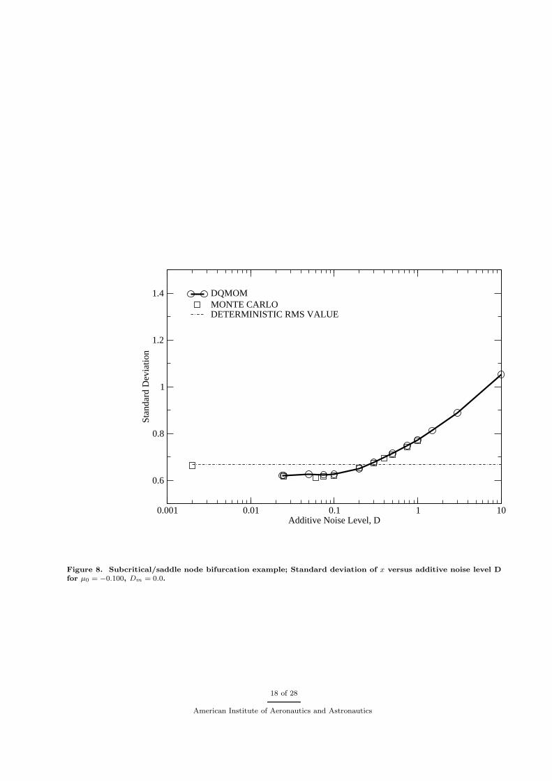
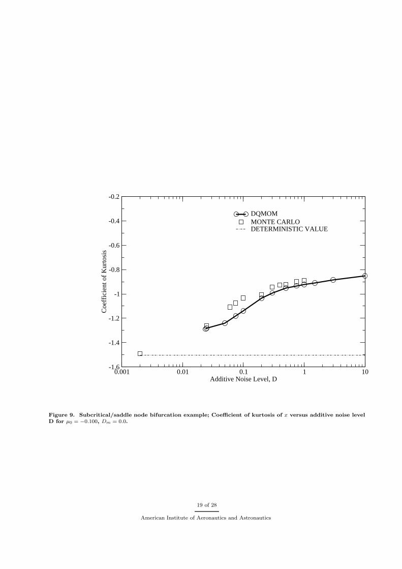
In the figures to follow, stationary values of standard deviation and coefficient of kurtosis are presentedfor a DQMOM solution with 11 quadrature points and for a numerical solution of Eqs. 32,33 using a forwardEuler-Maruyama time integration with a timestep of 0.0002. The statistics reported for the numerical solutionof Eqs. 32,33 are computed using direct Monte Carlo simulation with 10000 realizations. For the DQMOMsolution, all moments up to sixth order are closed along with the moments ( (r,s) ): (5,2),(2,6),(2,5),(1,6)and (0,7). The values for ω and b are chosen as 1 and 0.01 respectively.
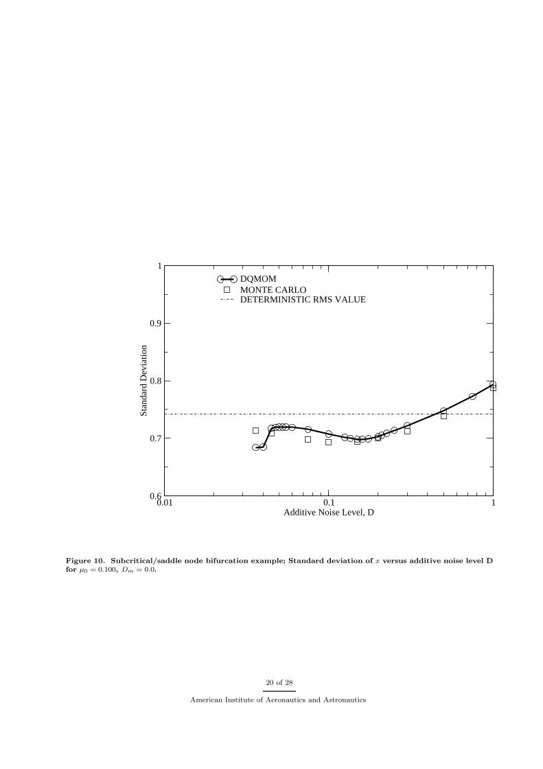
Figures 6-11 show the standard deviation and coefficient of kurtosis as a function of the additive noise levelD. Statistics for three different values of the mean of the bifurcation parameter µ0 are shown: µ0 = −0.275(Figs. 6,7) which, for the deterministic system, is below the saddle node value for µ0, µ0 = −0.100 (Figs. 8,9),which is in the region where two attractors exist, and µ0 = 0.100(Figs. 10,11) where the only attractor is thelarge amplitude LCO. In these figures the level of multiplicative noise Dm (random coefficient component)is zero. Also shown in Figs. 8- 11 are the corresponding values for the deterministic system, which exhibitsa limit cycle at µ = −0.100 and µ = 0.100. First note that in general there is very good agreement betweenthe DQMOM results and those from the numerical integration. As could be expected the standard deviationresults show better agreement. Two possible reasons for the differences in the kurtosis results are: 1) Ifthe evolution equations for the moments are written out, one will see that the equation which governs theevolution of the fourth moment ( d
dt < x4 >) will contain an 8th order moment, < x8 > which si not closedin the current DQMOM solution with 11 quadrature points and closed moments as stated above and 2) arigorous convergence study of the statistics computed with the Monte Carlo has not been conducted withregards to the number of realizations and the timestep hence it is possible that the higher order momentsare not completely converged for the Monte Carlo results. Overall, however, the agreement is good and thequalitative trends match for both methods. For example, the kurtosis is sub-Gaussian (negative) for eachvalue of µ0. While for µ0 = −0.275 the coefficient decreases with increasing additive noise level and appearsto be approaching an asymptotic value, for µ0 = −0.100 and µ0 = 0.100 the coefficient of kurtosis increaseswith increasing additive noise level. For both values of µ0 which correspond to cases where a stable LCOexists, µ0 = −0.100 and µ0 = 0.100, at low levels of noise the standard deviation versus noise level curveis flat. This would seem to indicate that for this level of additive noise, the system is mainly responding tothe LCO with little influence from the noise. This is not the case for µ0 = −0.275 where no LCO existsand the system is responding completely to the additive noise. Finally it appears that for µ0 = 0.100, thereis a local minimum in the standard deviation near D = 0.15 which is predicted by both the DQMOM andnumerical integration methods. The DQMOM also predicts a local minimum of the coefficient of kurtosisnear D = 0.06. This, however, is not predicted by the numerical integration.
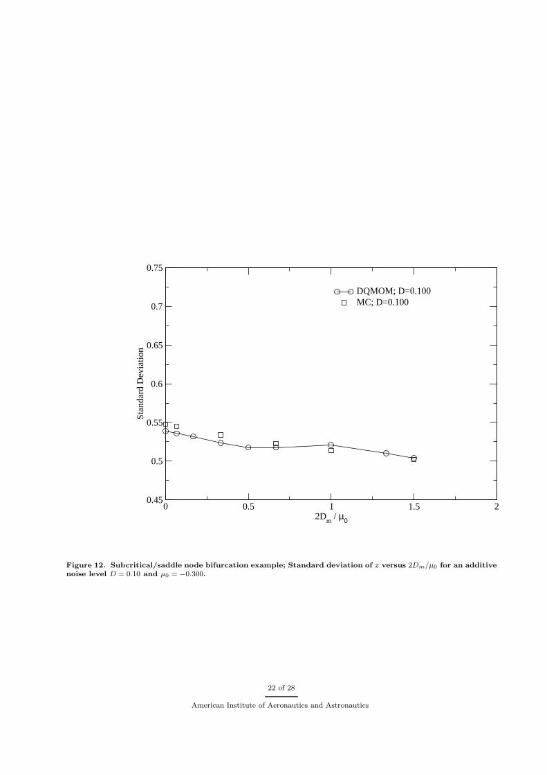
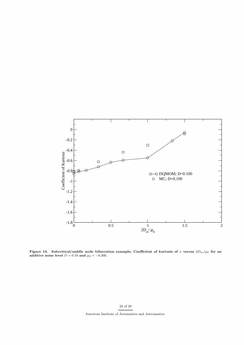
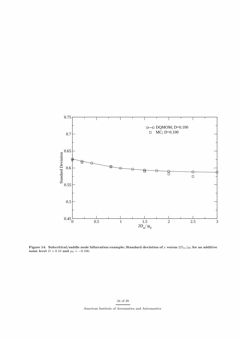
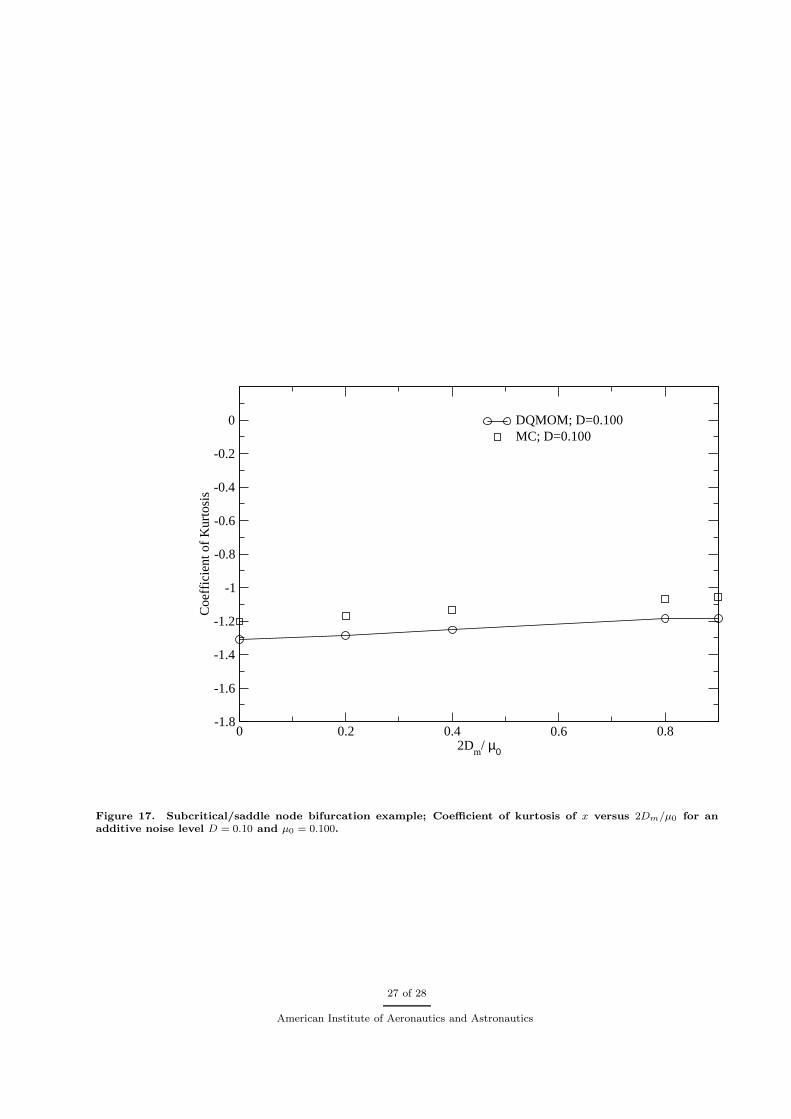
Shown in Figs. 12- 17 are the standard deviation and coefficient of kurtosis as a function of the ratio2Dm
µ0for three different values of µ0: -0.300,-0.100 and 0.100. The value of D for these figures is 0.10. Once
again the agreement between the DQMOM results and numerical integration results are good. Overall itappears that the standard deviation decreases with 2Dm/µ0 but is not a strong function of this parameter,at least for the additive noise level used in these figures (D = 0.100). Also, the coefficient of kurtosis resultsare sub-Gaussian and decrease in magnitude as the ratio 2Dm/µ0 increases. In particular, for µ0 = −0.300,which is below the saddle node value for µ0, the kurtosis seems to be approaching a switch from sub-Gaussianbehavior to super-Gaussian at or around 2Dm/µ0 = 1.5.
D. 4D Aeroelastic Typical Section Airfoil
The final example used to show the effectiveness of the DQMOM solution method is a dynamical systemrepresenting a typical section airfoil with pitch and plunge degrees of freedom in quasi-static subsonic flow.The pitch and plunge stiffnesses are considered to be nonlinear with a cubic spring for the plunge degree offreedom and a cubic and quintic spring for the pitch degree of freedom. If the constant for cubic term in thepitch degree of freedom is negative and the quintic is considered positive, the deterministic system exhibitsa subcritical Hopf bifurcation along with a saddle node bifurcation which results in hysteretic behavior. Thedynamic system can be written as (after nondimensionalization):
h′′
+ xαα′′ + ξhωh
ωαh′
+
(
ωh
ωα
)2 (
h + b2 Knlh
Khh
3)
= −πk
µ(h
′
+ kα) + L(τ) (35)
α′′ +xα
r2α
h′′
+ 2ξαα′ + α +Knl1
α
Kαα3 +
Knl2α
Kαα5 = π
e
b
k
µr2α
(h′
+ kα) + M(τ) (36)
7 of 28
American Institute of Aeronautics and Astronautics
As stated, we assume quasi-static aerodynamics with a lift curve slope of 2π.Here we will consider that the airfoil is subjected to turbulence in the vertical direction which we will treat
as an external random forcing, ie an additive white noise (delta correlated) process W (τ) which correspondsto L(τ) and M(τ) in Eqs. 35, 36. Future work will consider colored noise approximations for the turbulence.The corresponding Ito-type stochastic differential equations are
dh = ydτ (37)
dy = −(
[
2ξhωh
ωα+ π
k
µ
]
y +
(
ωh
ωα
)2(
h + b2 Knlh
Khh
3)
+ πk2
µα
)
dτ + σLdW (τ) (38)
dα = zdτ (39)
dz = −(
2ξαz +
[
1 − πe
b
k2
µr2α
]
α +Knl1
α
Kαα3 +
Knl2α
Kαα5 − π
e
b
k
µr2α
y
)
dτ + σMdW (τ) (40)
The Fokker-Planck equation which is to be solved using DQMOM is given by:
∂f
∂τ= − ∂
∂h{fy} +
∂
∂y
{
f
[
(
2ξhωh
ωα+ π
k
µ
)
y +
(
ωh
ωα
)2(
h + b2 Knlh
Khh
3)
+ πk2
µα
]}
− ∂
∂α{fz}+
∂
∂z
{
f
[
2ξαz +
(
1 − πe
b
k2
µr2α
)
α +Knl1
α
Kαα3 +
Knl2α
Kαα5 − π
e
b
k
µrα2
y
]}
+ (41)
1
2
∂2
∂y2{σ2
Lf} +1
2
∂2
∂z2{σ2
Mf}
The following values for the parameters are used in generating the results to follow: ωh
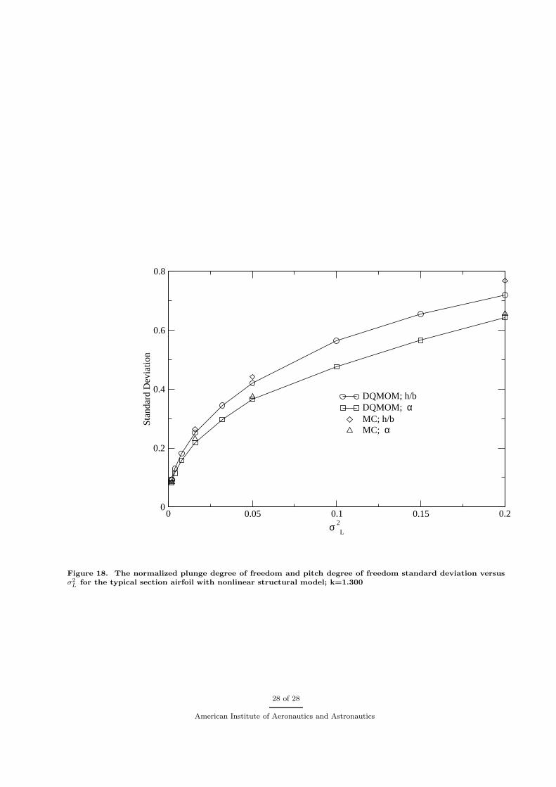
was fixed to be 0.1. For these parameter values, the deterministic system has a subcriticalHopf bifurcation at k = 1.475 and a saddle node bifurcation at k ≈ 1.460. Figure 18 shows the standarddeviation of α and h versus σ2
L for a value of k below the saddle node value, k = 1.30. The stationary valuesshown for the DQMOM solution are computed by solving the stationary form of the DQMOM discretizationof Eq. 41. Twelve quadrature points are used giving a total of 60 unknown weight and abscissa values.These unknowns are found by solving the set of 60 nonlinear algebraic equations using a modified Powellhybird method.28 The Monte Carlo results shown in Fig. 18 use 100000 realizations with a timestep of0.00025 for the Euler-Mayurama numerical integration of Eq. 40. Converged statistics for the Monte Carlosimulation took approximately 20 hours utilizing a MPI based parallel solution with 10 dual core Pentium4Xeon EM64T 3.2GHz processors. The stationary DQMOM solution, if provided with a reasonable initialguess for the nonlinear solver, took only seconds.
Future investigation of this problem will include computing the statistics for values of k which fall inthe hysteresis region (1.460 ≥ k < 1.475) and above the subcritical bifurcation point(linear flutter point)k = 1.475 and studying the effects of multiplicative noise in the problem parameters.
IV. Conclusions
A new method, the direct quadrature method of moments (DQMOM), is presented for the numericalsolution of the Fokker-Planck equations. In DQMOM, the probability density function is written as sum-mation of products of Dirac delta functions. The location of the quadrature abscissas in probability space(arguments of the delta function) become part of the solution and are obtained (along with the quadra-ture weights) as solutions of their evolution equations. These evolution equations are obtained through theFokker-Planck equation using constraints on the generalized moments of the stochastic processes. The useof the Dirac delta function results in a much simpler (over traditional weighted-residual methods) treatmentof nonlinear drift and diffusion terms.
In this paper the method has been used to compute moments for one-dimensional, two-dimensional andfour-dimensional processes which possess nonlinear stochastic differential equations. In the one-dimensionalproblem the stationary moments (second,fourth and sixth) computed using DQMOM compare well withanalytical solutions. The distribution for this problem is bimodal. The two-dimensional problems were the
8 of 28
American Institute of Aeronautics and Astronautics
noisy van der Pol oscillator and a problem which contains, for the deterministic system, both a saddle nodebifurcation and subcritical Hopf bifurcation. For both of these examples, stationary second and fourth ordermoments computed using DQMOM compared well with those computed using a Monte Carlo solution ofthe respective stochastic differential equations. Trends in the normalized moments with respect to additivenoise level and the bifurcation parameter are reported for the stochastic saddle node/subcritical problem forwhat appears to be the first time. These results could be useful in analyzing similar behavior for aeroelasticsystems which contain such stability properties.
Finally statistics are computed for a typical section airfoil in subsonic flow with nonlinear pitch andplunge stiffness (four-dimensional stochastic process). The airfoil is subjected to delta correlated randomforcing which approximates turbulence in the transverse component of flow velocity. The stationary standarddeviation results computed with the DQMOM approach for a reduced frequency value below the deterministicsaddle point compare well, for both the pitch and plunge degrees of freedom, with those computed using anumerical integration of the stochastic differential equations. Future investigation of this problem will includereduced frequency values within the hysteresis region and above the subcritical bifurcation (flutter) point.Also the effect of using colored noise approximations for the turbulence will be studied for this particularproblem which contains both a saddle node and subcritical bifurcation.
Acknowledgments
The authors would like to acknowledge The University of Oklahoma Supercomputing Center(OSCER)which provided supercomputing time to the authors enabling them to complete this work.
9 of 28
American Institute of Aeronautics and Astronautics
References
1Ibrahim, R., Orono, P., and Madaboosi, S., “Stochastic FLutter of a Panel Subjected to Random In-Plane Forces PartI: Two Mode Interaction,” AIAA Journal , Vol. 28, No. 4, 1990, pp. 694–702.
2Ibrahim, R. and Orono, P., “Stochastic flutter of a panel subjected to random in-plane forces. II - Two and three modenon-Gaussian solutions,” AIAA Paper 1990-986.
3Ibrahim, R., Beloiu, D., and Pettit, C., “Influence of Joint Relaxation on Deterministic and Stochastic Panel Flutter,”AIAA Journal , Vol. 43, No. 7, July 2005, pp. 1444–1454.
4Vaicaitis, R., Dowell, E., and Ventres, C., “Nonlinear Panel Response by a Monte Carlo Approach,” AIAA Journal ,Vol. 12, May 1974, pp. 685–691.
5Olson, M., “Some Flutter Solutions Using Finite Elements,” AIAA Journal , Vol. 8, 1970, pp. 747–752.6Pettit, C. L., “Uncertainty quantification in aeroelasticity: Recent results and research challenges.” Journal of Aircraft ,
Vol. 41, No. 5, September/October 2004, pp. 1217–1229.7Risken, H., The Fokker-Planck Equation: Methods of Solution and Applications, Springer-Verlag, New York, 2nd ed.,
1996.8Rodrıguez, R. and van Kampen, N., “Systematic treatment of fluctuations in a nonlinear osillator,” Physica, Vol. 85,
No. 2, 1976, pp. 347–362.9Weinstein, E. M. and Benaroya, H., “The van Kampen Expansion for the Fokker-Planck Equation of a Duffing Oscillator,”
Journal of Statistical Physics, Vol. 77, No. 3/4, 1994, pp. 667–679.10Voigtlaender, K. and Risken, H., “Solutions of the Fokker-Planck Equation for a Double-Well Potential in Terms of
Matrix Continued Fractions,” Journal of Statistical Physics, Vol. 40, No. 3/4, 1985, pp. 397–429.11Naess, A. and Hegstad, B., “Response Statistics of van der Pol Oscillators Excited by White Noise,” Nonlinear Dynamics,
Vol. 5, 1994, pp. 287–297.12Kumar, P. and Narayanan, S., “Solution of Fokker-Planck equation by finite element and finite difference methods for
nonlinear systems,” Sadhana, Vol. 31, No. 4, 2006, pp. 445–461.13Harrison, G. W., “Numerical Solution of the Fokker Planck Equation Using Moving Finite Elements,” Numerical Methods
for Partial Differential Equations, Vol. 4, 1988, pp. 219–232.14Jr., B. S. and Bergman, L., “On the Numerical Solution of the Fokker-Planck Equation for Nonlinear Stochastic Systems,”
Nonlinear Dynamics, Vol. 4, 1993, pp. 357–372.15Wojtkiewicz, S. and Bergman, L., “Numerical Solution of High Dimensional Fokker-Planck Equations,” Proceedings of
the 8th Specialty Conference on Probabilistic Mechanics and Structural Reliability, Paper PMC2000-167 , South Bend, IN,2000.
16Fox, R., Computational Models for Turbulent Reacting Flows, Cambridge University Press, 2003.17Marchisio, D. and Fox, R., “Solution of population balance equations using the direct quadrature method of moments,”
Journal of Aerosol Science, Vol. 36, 2005, pp. 43–73.18Fan, R., Marchisio, D., and Fox, R., “Application of the direct quadrature method of moments to polydisperse, gas-solid
fluidized beds,” Powder Technology , Vol. 139, 2004, pp. 7–20.19Vedula, P. and Fox, R. O., “Direct quadrature method of moments for the Boltzmann equation,” Submitted to Journal
of Statistical Physics.20Attar, P. J. and Vedula, P., “Direct Quadrature Method of Moments Solution of the Fokker-Planck Equation,” Journal
of Sound and Vibration, 2008, doi:10.1016/j.jsv.2008.02.037.21Petzold, L. R., “A description of DASSL: A differential/algebraic system solver,,” IMACS Trans. Scientific Computing ,
edited by S. S. et al., Vol. 1, North-Holland, Amsterdam, 1993, pp. 65–68.22Brenan, K., Campbell, S., and Petzold, L., Numerical solution of initial-value problems in differential-algebraic equations,
North Holland, Amsterdam, 1989.23Brown, P. N., Hindmarsh, A. C., and Petzold, L. R., “Consistent Initial Condition Calculation for Differential-Algebraic
Systems,” SIAM Journal on Scientific Computing , Vol. 19, No. 5, September 1998, pp. 1495–1512.24To, C., “A Statistical Non-Linearization Technique in Structural Dynamics,” Journal of Sound and Vibration, Vol. 161,
No. 3, 1993, pp. 543–548.25Strogatz, S. H., Nonlinear Dynamics and Chaos, Addison-Wesley Publishing Company, 1998.26Attar, P., Dowell, E., and Tang, D., “Modeling Aerodynamic Nonlinearities for Two Aeroelastic Configurations: Delta
Wing and Flapping Flag,” AIAA Paper 2003-1402 April 7-10, 2003.27Probabilistic Structural Dynamics: Advanced Theory and Applications, McGraw-Hill, New York, 1995.28Powell, M., “A Hybrid Method for Nonlinear Equations,” Numerical Methods for Nonlinear Algebraic Equations, edited
by P. Rabinowitz, Gordon and Breach Science, London, 1970, pp. 87–144.
10 of 28
American Institute of Aeronautics and Astronautics
Figure 5. Fokker-Planck for the van der Pol equation; Fourth moment of x versus the noise intensity level D.
15 of 28
American Institute of Aeronautics and Astronautics
0.01 0.1 1 10Additive Noise Level, D
0.25
0.5
0.75
1
1.25
Stan
dard
Dev
iatio
n
DQMOMMONTE CARLO
Figure 6. Subcritical/saddle node bifurcation example; Standard deviation of x versus additive noise level Dfor µ0 = −0.275, Dm = 0.0.
16 of 28
American Institute of Aeronautics and Astronautics
0.01 0.1 1 10Additive Noise Level, D
-1
-0.9
-0.8
-0.7
-0.6
-0.5
-0.4
Coe
ffic
ient
of
Kur
tosi
s
DQMOMMONTE CARLO
Figure 7. Subcritical/saddle node bifurcation example; Coefficient of kurtosis of x versus additive noise levelD for µ0 = −0.275, Dm = 0.0.
17 of 28
American Institute of Aeronautics and Astronautics
0.001 0.01 0.1 1 10Additive Noise Level, D
0.6
0.8
1
1.2
1.4
Stan
dard
Dev
iatio
n
DQMOMMONTE CARLODETERMINISTIC RMS VALUE
Figure 8. Subcritical/saddle node bifurcation example; Standard deviation of x versus additive noise level Dfor µ0 = −0.100, Dm = 0.0.
18 of 28
American Institute of Aeronautics and Astronautics
0.001 0.01 0.1 1 10Additive Noise Level, D
-1.6
-1.4
-1.2
-1
-0.8
-0.6
-0.4
-0.2
Coe
ffic
ient
of
Kur
tosi
s
DQMOMMONTE CARLODETERMINISTIC VALUE
Figure 9. Subcritical/saddle node bifurcation example; Coefficient of kurtosis of x versus additive noise levelD for µ0 = −0.100, Dm = 0.0.
19 of 28
American Institute of Aeronautics and Astronautics
0.01 0.1 1Additive Noise Level, D
0.6
0.7
0.8
0.9
1
Stan
dard
Dev
iatio
n
DQMOMMONTE CARLODETERMINISTIC RMS VALUE
Figure 10. Subcritical/saddle node bifurcation example; Standard deviation of x versus additive noise level Dfor µ0 = 0.100, Dm = 0.0.
20 of 28
American Institute of Aeronautics and Astronautics
0.01 0.1 1Additive Noise Level, D
-1.6
-1.4
-1.2
-1
-0.8
Coe
ffic
ient
of
Kur
tosi
s
DQMOMMONTE CARLODETERMINISTIC VALUE
Figure 11. Subcritical/saddle node bifurcation example; Coefficient of kurtosis of x versus additive noise levelD for µ0 = 0.100, Dm = 0.0.
21 of 28
American Institute of Aeronautics and Astronautics
0 0.5 1 1.5 22D
m / µ0
0.45
0.5
0.55
0.6
0.65
0.7
0.75
Stan
dard
Dev
iatio
n
DQMOM; D=0.100MC; D=0.100
Figure 12. Subcritical/saddle node bifurcation example; Standard deviation of x versus 2Dm/µ0 for an additivenoise level D = 0.10 and µ0 = −0.300.
22 of 28
American Institute of Aeronautics and Astronautics
0 0.5 1 1.5 22D
m/ µ0
-1.8
-1.6
-1.4
-1.2
-1
-0.8
-0.6
-0.4
-0.2
0
Coe
ffic
ient
of
Kur
tosi
s
DQMOM; D=0.100MC; D=0.100
Figure 13. Subcritical/saddle node bifurcation example; Coefficient of kurtosis of x versus 2Dm/µ0 for anadditive noise level D = 0.10 and µ0 = −0.300.
23 of 28
American Institute of Aeronautics and Astronautics
0 0.5 1 1.5 2 2.5 32D
m/ µ0
0.45
0.5
0.55
0.6
0.65
0.7
0.75
Stan
dard
Dev
iatio
n
DQMOM; D=0.100MC; D=0.100
Figure 14. Subcritical/saddle node bifurcation example; Standard deviation of x versus 2Dm/µ0 for an additivenoise level D = 0.10 and µ0 = −0.100.
24 of 28
American Institute of Aeronautics and Astronautics
0 0.5 1 1.5 2 2.5 32D
m/ µ0
-1.8
-1.6
-1.4
-1.2
-1
-0.8
-0.6
-0.4
-0.2
0
Coe
ffic
ient
of
Kur
tosi
s
DQMOM; D=0.100MC; D=0.100
Figure 15. Subcritical/saddle node bifurcation example; Coefficient of kurtosis of x versus 2Dm/µ0 for anadditive noise level D = 0.10 and µ0 = −0.100.
25 of 28
American Institute of Aeronautics and Astronautics
0 0.2 0.4 0.6 0.82D
m/ µ0
0.45
0.5
0.55
0.6
0.65
0.7
0.75
Stan
dard
Dev
iatio
n
DQMOM; D=0.100MC; D=0.100
Figure 16. Subcritical/saddle node bifurcation example; Standard deviation of x versus 2Dm/µ0 for an additivenoise level D = 0.10 and µ0 = 0.100.
26 of 28
American Institute of Aeronautics and Astronautics
0 0.2 0.4 0.6 0.82D
m/ µ0
-1.8
-1.6
-1.4
-1.2
-1
-0.8
-0.6
-0.4
-0.2
0
Coe
ffic
ient
of
Kur
tosi
s
DQMOM; D=0.100MC; D=0.100
Figure 17. Subcritical/saddle node bifurcation example; Coefficient of kurtosis of x versus 2Dm/µ0 for anadditive noise level D = 0.10 and µ0 = 0.100.
27 of 28
American Institute of Aeronautics and Astronautics
0 0.05 0.1 0.15 0.2
σ 2
L
0
0.2
0.4
0.6
0.8
Stan
dard
Dev
iatio
n
DQMOM; h/bDQMOM; αMC; h/bMC; α
Figure 18. The normalized plunge degree of freedom and pitch degree of freedom standard deviation versusσ2
Lfor the typical section airfoil with nonlinear structural model; k=1.300
28 of 28
American Institute of Aeronautics and Astronautics