Diversity and Frame Invariance Characteristics in Particle Swarm Optimization with and without Digital
Pheromones
Vijay Kalivarapu1 and Eliot Winer2 Virtual Reality Applications Center, Iowa State University, Ames, IA, 50011, USA
Academic problems for testing optimization methods are widely criticized for not being a good representative of real world problems. Due to the unavailability of publishable proprietary information from industries they collaborate with, researchers tend to simulate complex problems by using ‘n-dimensional’ multi-modal and/or multi-objective academic test problems for evaluating optimization methods developed. Most of these benchmarking test problems can be decomposed and solved as ‘n’ 1-dimensional optimization problems, rendering them as ineffective representation of real-world problems. However, studies show that coordinate rotation of test problems through an arbitrary angle makes design variables dependent on each other and cannot easily be decomposed into simpler problem chunks. Test problems formulated with coordinate rotation therefore will represent a realistic test bed for evaluating the performance of an optimization routine. However with coordinate rotation, the complexity of the problems potentially increases from O(nn) to O(exp(n ln n)) imposing performance loss on the optimization method that solves the problem. In this paper, the authors attempted to investigate whether coordinate rotation affects the performance characteristics of the digital pheromone implementation of Particle Swarm Optimization (PSO). In particular, two characteristics - swarm diversity with different random number schemes for the velocity vector, and frame invariance with rotational problems are studied and reported. In other words, the authors intended to evaluate whether PSO with digital pheromones is truly capable of solving complex problems.
I. Introduction article Swarm Optimization (PSO) 1,2 is a population based heuristic method retaining many characteristics of evolutionary search algorithms such as a GA. It is a recent addition to global search
methods 3 and one of its key features is its simplicity in implementation due to a small number of parameters to adjust 4, 5. In a regular PSO, an initial randomly generated population swarm (a collection of particles) propagates towards the global optimum over a series of iterations. Each particle in the swarm explores the design space based on the information provided by two members – the best position of a swarm member in its history trail (pBest), and the best position attained by all particles (gBest) until that iteration. This information is used to generate a velocity vector indicating a search direction towards a promising design point, and the location of each swarm member is updated. The drawback of this approach is that information from these two members alone is not sufficient for the swarm to propagate toward the global optimum efficiently. This either could cause the swarm to lock into a local minimum or take a long time to approach the global optimum. Previous work by the authors demonstrated promising performance improvement of PSO in terms of increased solution efficiency, accuracy, and reliability through
1 Postdoctoral Research Associate and author of correspondence, Department of Mechanical Engineering, Human Computer Interaction, Virtual Reality Applications Center, 2274 Howe Hall, Iowa State University, Ames, IA, 50011, USA, Student Member. Email: [email protected], [email protected], Phone: 515-294-3092, Fax: 515-294-5530. 2 Associate Professor, Department of Mechanical Engineering, Human Computer Interaction, Virtual Reality Applications Center, 2274 Howe Hall, Iowa State University, Ames, IA, 50011, USA, Member.
P
51st AIAA/ASME/ASCE/AHS/ASC Structures, Structural Dynamics, and Materials Conference<BR> 18th12 - 15 April 2010, Orlando, Florida
implementing digital pheromones in PSO 6. Sections I-A through I-C explain the workings of a basic PSO and digital pheromone implementation of PSO. A. Particle Swarm Optimization
PSO shares many characteristics of evolutionary search algorithms such as Genetic Algorithms (GA) and Simulated Annealing (SA) – a) Initialization with a population of random solutions, b) Design space search for optimum through updating generations and c) Update based on previous generations 7. The success of the algorithm has brought substantial attention among the research community in the recent past 8, 9. The working of the algorithm is based on a simplified social model similar to the swarming behavior exhibited by insects and birds. In this analogy, a swarm member uses its own memory and the behavior of the rest of the swarm to determine the suitable location of food (global optimum). The algorithm iteratively updates the direction of the swarm movement toward the global optimum. The mathematical formulation of the method is given in Equations (1) and (2).
(1)
(2)
witeriter ww λ×=+1 (3)
Equation (1) represents the velocity vector update, representing the direction and magnitude of ith swarm member in a basic PSO in iteration ‘iter’. Each successive iteration is represented by ‘iter+1’. The square braces in equations (1) and (2) indicate an array meaning that the corresponding value (e.g., pBest) is computed
for each design variable. and are unique random numbers generated between 0 and 1 for pBest and gBest components separately for each swarm member in each iteration. The parentheses in randp() and randg() indicate that they are random number generating functions within the computer code. This ensures swarm diversity, meaning that the search is not linear in an n-dimensional space. More about swarm diversity can be obtained from 10. c1 and c2 are user definable confidence parameters. Typically, these are set to values of 2.0. ‘pBest’ represents the best position of the particle in its history trail, and ‘gBest’ represents the best particle location in the entire swarm. witer is termed “inertia” weight, and is used to control the impact of a particle’s previous velocity on the calculation of the current velocity vector. A large value for witer facilitates global exploration, which is particularly useful in the initial stages of an optimization. A small value allows for more localized searching, which is useful as the swarm moves toward the neighborhood of the optimum 11, 12. These characteristics are attributed to the swarm by implementing a decay factor, λw for the inertia weight, as shown in equation (3). Equation (2) denotes the updated swarm location in the design space.
In addition to the originally developed PSO algorithm, significant enhancements have been proposed such as: a) mutation factors for better design space exploration 13, 14, b) methods for constraint handling 15,
16, c) parallel implementation 17, 18, d) methods for solving multi-objective optimization problems 19, e) methods for solving mixed discrete, integer and continuous variables 20.
B. Digital Pheromones
Pheromones are chemical scents produced by insects to communicate with each other to find a suitable food source, nesting location, etc. The stronger the pheromone, the more the insects are attracted to the path. A digital pheromone is analogous to an insect generated pheromone in that they are the markers to determine whether or not an area is promising for further investigation. One of the well-known applications of digital pheromones is its use in the automatic adaptive swarm management of Unmanned Aerial Vehicles (UAVs) 21, 22. In this research, the UAVs are automatically guided towards a specific zone or target through releasing digital pheromones in a virtual environment, thereby reducing the requirement of humans physically controlling from ground stations. Other applications of digital pheromones include ant colony optimization for solving minimum cost paths in graphs 23, 24 solving network communication
problems 25. The concept of digital pheromones is considerably new 26 and has not yet been explored to its full potential for investigating n-dimensional design spaces for locating an optimum.
In a regular PSO algorithm, the swarm movement obtains design space information from only two components – pBest and gBest. When coupled with an additional pheromone component, the swarm is essentially presented with more information for design space exploration and has a potential to reach the global optimum faster.
C. Overview of Digital Pheromones in PSO
In a basic PSO algorithm, the velocity vector governs the swarm movement computed in Equation (1). Each swarm member uses information from its previous best and the best member in the entire swarm at any iteration.
Figure 1. (Left) Particle movement in basic PSO, (Right) Particle movement in digital pheromone PSO
However, multiple pheromones released by the swarm members could provide more information on
promising locations within the design space when the information obtained from pBest and gBest are insufficient or inefficient. Figure 1 (left) displays a scenario of a swarm member’s movement whose direction is guided by pBest and gBest alone. The particle’s position in the previous iteration is denoted by Pi-1, and the current position is denoted by Pi. Vi-1 indicates the particle’s velocity in the previous iteration and Vi denotes the velocity in the current iteration. If c1 >> c2, the particle is attracted primarily towards its personal best position. On the other hand, if c2 >> c1, the particle is strongly attracted to the gBest position. In the scenario dominated by c2, as presented in figure 3 (left), neither pBest nor gBest leads the swarm member to the global optimum, at the very least, not in this iteration adding additional computation to find the optimum. Figure 1 (right) shows the effect of implementing digital pheromones into the velocity vector. An additional target pheromone component potentially causes the swarm member to result in a direction different from the combined influence of pBest and gBest thereby increasing the probability of finding the global optimum. Figure 2 summarizes the general procedure for PSO, with steps involving digital pheromones highlighted. The method initialization is similar to a basic PSO except that 50% percent of the swarm within the design space is randomly selected to release pheromones in the first iteration. This parameter is user-defined, but experimentation has shown 50% to be a good default value. For subsequent iterations, each swarm member that realizes any improvement in the actual objective function value is allowed to release a pheromone.
Evaluate fitness value of each swarm member
Store pBest and gBest
Start Iterations
Decay digital pheromones in the design space (if any)
Populate particle swarm with random initial values
Merge pheromones based on relative distance between each
1st iteration?
Find target pheromone toward which the swarm moves
Update velocity vector and position of the swarm
Converged?
STOP! No Yes
Randomly chosen 50% of swarm release pheromones Only improved particles release pheromones
No
Yes
Figure 2 Overview of PSO with Digital Pheromones
Pheromones from the current as well as the past iterations that are close to each other in terms of the design variable value are merged into a new pheromone location. Therefore, a pheromone pattern across the design space is created, while keeping the number of pheromones manageable. In addition, the digital pheromones are decayed every iteration just as natural pheromones. Based on the current pheromone level and its position relative to a particle, a ranking process is used to select a target pheromone for each particle in the swarm. This target position towards which a particle will be attracted is called the target pheromone and added as an additional velocity vector component to pBest and gBest. This procedure is continued until a prescribed convergence criterion is satisfied. A detailed account of this procedure is fully explained in the previous work by authors 6, and is not described in this paper to maintain conciseness. The new velocity vector update equation is shown in equation (4).
(4)
, and are unique random numbers generated between 0 and 1 for pBest, gBest and target pheromone components separately for each swarm member in each iteration. The parentheses in randp( ), randg( ) and randT( ) indicate that they are random number generating functions within the computer code. These values are updated in each iteration within the velocity vector equation, resulting in improved swarm diversity. The square braces in equation (4) indicate an array meaning that the corresponding value (e.g., TargetPheromone) is computed for all design variables.
c3 is a user defined confidence parameter for the pheromone component of the velocity vector similar to c1 and c2 in a basic PSO. c3 combines the knowledge from the cognitive and social components of the velocity of a particle, and complements their deficiencies. In a basic PSO, the particle swarm does not have a memory of the entire path traversed in the design space apart from the best position of an individual particle (pBest) and the best member’s position in the entire swarm (gBest). The target pheromone component addresses this issue. It is a container that functionally stores the trail path of the swarm and utilizes the best features of pBest and gBest in steering towards a promising location in the design space. The confidence parameter c3 determines the extent of influence a target pheromone can have on the swarm when the information from pBest and gBest alone are not sufficient or efficient to determine a particle’s next move. The use of the target pheromone relies heavily on pBest and gBest. If c3 = 0, there is no influence of pheromones and the swarm behaves as if in a regular PSO. If either of c1 or c2 is 0 and c3 > 0, then the target pheromone location is essentially determined only by the non-zero component of pBest or gBest and propagated into the velocity vector. This creates a bias thereby doubling the influence of non-zero pBest or gBest components on the swarm. This means that the swarm either explores or exploits the design space with double the intensity, either of which will prevent the swarm from converging. It is therefore essential that the influence of pBest and gBest be balanced (i.e. equal) for the pheromone component to provide accurate assistance in reaching the optimum. Although analytical determination of a value for c3 is out of the scope of this research, an empirical value has been determined through experimentation. A value between 2.0 and 5.0 has shown good performance characteristics and solved a variety of problems. An inertia weight, wi of value 1.0 is initially chosen to preserve the influence of the velocity vector from previous iterations, and gradually decreased using an inertia weight decay factor similar to the one used in a basic PSO. Digital pheromone implementation in PSO yielded promising performance improvements in terms of solution accuracy, efficiency and reliability on standard benchmarking test problems. Further enhancements in performance were realized through developing parallel cluster computing schemes 27, 28. Two different Graphics Processing Unit (GPU) implementations were also made 29, 30 to leverage the agility of current day graphics cards. Also, a quantitative assessment has also been made through statistical hypothesis testing 31. D. Issues with Academic type Problems Thus far, the methods developed by the authors were tested on purely academic type problems (e.g., De-Jong’s functions, Ackley’s path function, Griewangk’s function, Rastrigin’s function etc).
€
F(X) = f i(xi)i= 0
n
∑ (5)
Most of these test functions are decomposable into ‘n’ 1-D problems. Equation (5) is an illustration of an n-dimensional function that can be decomposed into ‘n’ functions not necessarily identical. The design variables represented by xi in such functions can be termed as independent, making it possible to optimize the function in a series of ‘n’ independent optimization procedures. Although highly multi-modal academic type problems are quite complex, a closer look reveals that the function can be decomposed into ‘n’ 1-D problems, as shown in the Ackley’s path function in equation (6). The combination of the solutions obtained from solving each 1-D problem then forms the solution vector to the original F(X).
(6)
Real-world problems do not necessarily present themselves as decomposable, and therefore optimization methods should be robust enough to be able to solve them in spite of having dependent design variables. Since publishable industry problems are not always available to academicians and researchers, it will be useful to formulate academic problems to simulate real-world problems. One method to do this is through coordinate rotation. E. Coordinate Rotation Coordinate rotation is not a new concept. Matrix rotation operations, for instance, are extensively used in various fields of physics, computer graphics, etc. A two-dimensional rotational transformation is shown in equation (7), where two variables X and Y are rotated by an angle θ resulting in transformed variables X’ and Y’.
€
X 'Y '⎡
⎣ ⎢
⎤
⎦ ⎥ =
cos(θ) sin(θ)−sin(θ) cos(θ)⎡
⎣ ⎢
⎤
⎦ ⎥ ×
XY⎡
⎣ ⎢ ⎤
⎦ ⎥ (7)
It might seem counter-intuitive how rotations can assist optimization routines. Figure (3) illustrates a hypothetical two variable objective function contour aligned to coordinate axes. The improvement in objective function values in this case is much simpler and faster as the optimization routine progresses. However, when the design variable axes are rotated by an angle (described by a rotation matrix M), the improvement in objective function values is much smaller and slower. This can be thought of as an optimization routine requiring more iterations and hence more objective function evaluations. In population based methods such as a GA or PSO, the complexity in solving such rotated problems is much higher when compared to problems that are decomposable and axes aligned.
Figure 3. (Left) Improvement in objective function value easier when design space is aligned to coordinate
axes, (Right) Smaller improvements realized when coordinate axes are rotated
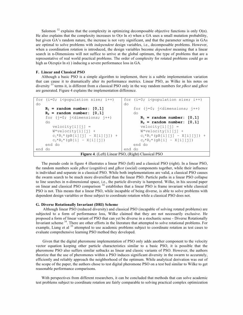
Salomon 32 explains that the complexity in optimizing decomposable objective functions is only O(n). He also explains that the complexity increases to O(n ln n) when a GA uses a small mutation probability, but given GA’s random nature, the increase is not very significant, and that the parameter settings in GAs are optimal to solve problems with independent design variables, i.e., decomposable problems. However, when a coordination rotation is introduced, the design variables become dependent meaning that a linear search in n-Dimensions will not suffice to arrive at the global optimum, the type of problems that are a representative of real world practical problems. The order of complexity for rotated problems could go as high as O(exp(n ln n) ) inducing a severe performance loss in GA. F. Linear and Classical PSO Although a basic PSO is a simple algorithm to implement, there is a subtle implementation variation that can cause it to dramatically alter its performance metrics. Linear PSO, as Wilke in his notes on diversity 33 terms it, is different from a classical PSO only in the way random numbers for pBest and gBest are generated. Figure 4 explains the implementation difference. for (i=0; i<population size; i++) do R1 = random number: [0,1] R2 = random number: [0,1] for (j=0; j<dimensions; j++) do velocity[i][j] = W*velocity[i][j] + c1*R1*(pB[i][j] – X[i][j]) + c2*R2*(gB[i] – X[i][j]) end do end do
for (i=0; i<population size; i++) do for (j=0; j<dimensions; j++) do R1 = random number: [0,1] R2 = random number: [0,1] velocity[i][j] = W*velocity[i][j] + c1*R1*(pB[i][j] – X[i][j]) + c2*R2*(gB[i] – X[i][j]) end do end do
Figure 4. (Left) Linear PSO, (Right) Classical PSO The pseudo code in figure 4 illustrates a linear PSO (left) and a classical PSO (right). In a linear PSO, the random numbers scale pBest (cognitive) and gBest (social) components together, while their influence is individual and separate in a classical PSO. While both implementations are valid, a classical PSO causes the swarm search to be much more diversified than the linear PSO. Particle paths in a linear PSO collapse to line searches in n-dimensional space, i.e., the particle diversity is hampered. Wilke, in his second paper on linear and classical PSO comparison 34 establishes that a linear PSO is frame invariant while classical PSO is not. This means that a linear PSO, while incapable of being diverse, is able to solve problems with dependent design variables or those subject to coordinate rotation while a classical PSO does not. G. Diverse Rotationally Invariant (DRI) Scheme
Although linear PSO (reduced diversity) and classical PSO (incapable of solving rotated problems) are subjected to a form of performance loss, Wilke claimed that they are not necessarily exclusive. He proposed a form of linear variant of PSO that can yet be diverse in a stochastic sense - Diverse Rotationally Invariant scheme 34. There are other efforts in the literature that attempted to solve rotational problems. For example, Liang et al 35 attempted to use academic problems subject to coordinate rotation as test cases to evaluate comprehensive learning PSO method they developed. Given that the digital pheromone implementation of PSO only adds another component to the velocity vector equation keeping other particle characteristics similar to a basic PSO, it is possible that the pheromone PSO also suffers similar setbacks as linear and classic variants of PSO. However, the authors theorize that the use of pheromones within a PSO induces significant diversity in the swarm to accurately, efficiently and reliably approach the neighborhood of the optimum. While analytical derivation was out of the scope of the paper, the authors chose to test digital pheromone PSO on a test bed similar to Wilke to get reasonable performance comparisons. With perspectives from different researchers, it can be concluded that methods that can solve academic test problems subject to coordinate rotation are fairly comparable to solving practical complex optimization
problems. The authors attempted to evaluate PSO with digital pheromones to solve academic problems subject to coordinate rotation and presented the findings in this paper.
II. Methodology
A. Orthogonal and Rotational Matrices An orthogonal matrix is a square matrix of the form n x n with its columns or rows forming unit
orthogonal vectors. A matrix is considered orthogonal if it follows two rules: a) It’s transpose is equal to its inverse, and b) it’s determinant is ±1.0 shown in equations (8) and (9).
[M]Tx[M]-1 = [M]-1x[M]T = I
⇒ [M]T = [M]-1
(8)
|M| = ±1.0 (9)
Those orthogonal matrices that result in a determinant of +1.0 are called as ‘special orthogonal group’ and can act as rotational matrix. More on orthogonal matrices can be found here 36.
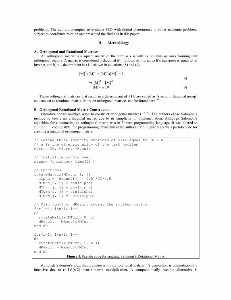
B. Orthogonal Rotational Matrix Construction Literature shows multiple ways to construct orthogonal matrices 32, 37. The authors chose Salomon’s
method to create an orthogonal matrix due to its simplicity in implementation. Although Salomon’s algorithm for constructing an orthogonal matrix was in Fortran programming language, it was altered to suit to C++ coding style, the programming environment the authors used. Figure 5 shows a pseudo code for creating a rotational orthogonal matrix.
// Define three identity matrices of size equal to ‘n x n’ // n is the dimensionality of the test problem Matrix ME, MTurn, MResult // Initialize random seed srand( (unsigned) time(0) ) // Functions rotateMatrix(MTurn, i, j) alpha = (drand48() – 0.5)*PI*0.5 MTurn[i, i] = cos(alpha) MTurn[j, j] = cos(alpha) MTurn[i, j] = sin(alpha) MTurn[j, i] = -sin(alpha) // Main routine. MResult stores the rotated matrix for(i=1; i<n-1; i++) do rotateMatrix(MTurn, 0, i) MResult = MResult*MTurn end do for(i=1; i<n-2; i++) do rotateMatrix(MTurn, i, n-1) MResult = MResult*MTurn end do
Figure 5. Pseudo code for creating Salomon’s Rotational Matrix
Although Salomon’s algorithm constructs a pure rotational matrix, it’s generation is computationally intensive due to (n-1)*(n-2) matrix-matrix multiplication. A computationally feasible alternative is
discussed in Wilke’s notes on frame invariance 34, albeit lesser accurate than Salomon’s algorithm. For this paper, Salomon’s orthogonal matrix was used to create a pure rotation matrix once per trial run to rotate the coordinate frame of the objective function. Wilke’s rotational matrix was used once per iteration for each design variable to implement a Diverse Rotationally Invariant (DRI) scheme for PSO. The results section (Section III) explains the need for using DRI scheme.
C. Rotation of Objective Function Coordinate Frames An orthogonal rotational matrix M of size n x n was pre-constructed for each problem and stored,
where ‘n’ indicates the dimensionality of the test problem. The design variable vector is pre-multiplied by the rotational matrix to result in a new set of rotated design variable vector, as shown in equation (10).
€
m1x1 . . m1xn. . . .. . . .
mnx1 . . mnxn
⎡
⎣
⎢ ⎢ ⎢ ⎢
⎤
⎦
⎥ ⎥ ⎥ ⎥
×
x1..xn
⎡
⎣
⎢ ⎢ ⎢ ⎢
⎤
⎦
⎥ ⎥ ⎥ ⎥
=
y1..yn
⎡
⎣
⎢ ⎢ ⎢ ⎢
⎤
⎦
⎥ ⎥ ⎥ ⎥
(10)
Therefore if [X] = [x1, x2, …, xn]T, the rotational matrix transforms the design variables to form [Y] =
[y1, y2, …, yn]T, where yi = mix1x1 + mix2x2 + … + mixnxn, i = 1, 2, …, n. The matrix [M] is pure rotation, and is constructed once per trial run with randomized initial values for rotational angles. The design variable vector [Y] is used instead of [X] every time the fitness value is computed in the optimization routine. The use of rotated design variable vector only changes the coordinate axes against which the objective function is aligned and does not alter the shape of the objective function in any manner.
III. Results A. Evaluating Digital Pheromone PSO for Rotational Problems
Wilke has analytically established in his work that a classical implementation of basic PSO is rotationally variant. That means, it induces performance loss on problems with dependent design variables or rotational problems. Similarly, a linear implementation of basic PSO lacks diversity characteristics. That is, particle search reduce to line search in n-dimensional design spaces. Digital pheromone PSO is likely subjected to similar setbacks but the authors theorize that pheromones add significant diversity to the swarm to accurately, efficiently and reliably approach the neighborhood of the optimum. While analytical derivation was out of the scope of the paper, the authors chose to test digital pheromone PSO on a similar test bed as Wilke to get unbiased performance comparisons.
As such, a variety of scenarios were considered for testing. Parallels were drawn against linear and
classic basic PSO implementations. Also, solution accuracies of basic and digital pheromone PSO were compared in rotated and un-rotated coordinate frames as well. In total, 24 scenarios were tested and figure 6 shows the layout.
Figure 6. Layout for the scenarios tested to evaluate digital pheromone PSO with coordinate rotation
B. PSO Heuristics The heuristics: (a) Cap on the velocity vector values, (b) Particle position limits as a function of design
variable bounds, and (c) dynamic inertia weight, may interfere with how PSO performs upon coordinate rotation. Therefore, one of the scenario for testing included no PSO heuristics for basic and digital pheromone implementations. A scenario with heuristics was also included to check how a fully functional digital pheromone PSO measured against basic PSO for rotational problems. Un-rotated functions were also included in the testing scenario to compare solution accuracies with rotated problems.
C. Test Problem Settings
Three 30 dimensional problems were used as test cases for executing all 24 scenarios listed in section III A. Table 1 Test problem Matrix shows the list of test problems along with their published solutions and design variable bounds. Full mathematical descriptions for these problems can be found in 38-40.
Table 1 Test problem Matrix
Problem Test Problem Published Solution Dimensions Design variable bounds 1 Quadric function 0.000 30 ± 100.0 2 Ackley’s path function 0.000 30 ± 30.0 3 Griewank function 0.000 30 ± 500.0
The digital pheromone parameters c3 = 5.0 and a pheromone decay λp = 5% as established previously by
the authors were used in all scenarios. These parameter settings were upheld for scenarios with and without PSO heuristics because they are the underlying characteristics of a digital pheromone model. However, the move limit decay λML of 5%, which is used for velocity vector computation was not included in the scenario without PSO heuristics. A total of 20 trial runs were conducted for all scenarios and the swarm size was set as 20 to be consistent with Wilke’s implementation of PSO. The problems tested were considered converged when the difference in solutions was within a tolerance of 0.01 for ten consecutive iterations.
The computing platform used was an eight-core Intel Xeon processor (3.2 GHz) Linux workstation with
RedHat Enterprise Linux 5 edition operating system. The code was however single threaded and only one
Basic PSO
(without and with heuristics)
Unrotated
Linear
Classic
DRI
Rotated
Linear
Classic
DRI
Pheromone PSO
(without and with heuristics)
Unrotated
Linear
Classic
DRI
Rotated
Linear
Classic
DRI
processor core was used for testing the performance. The system memory was 4GB DDR2. The PSO algorithm was implemented in C++ programming language.
D. Comparison of Results from Different Scenarios
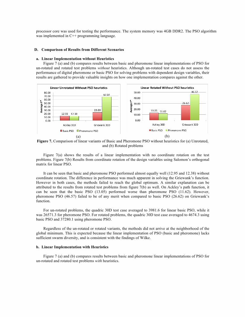
a. Linear Implementation without Heuristics Figure 7 (a) and (b) compares results between basic and pheromone linear implementations of PSO for
un-rotated and rotated test problems without heuristics. Although un-rotated test cases do not assess the performance of digital pheromone or basic PSO for solving problems with dependent design variables, their results are gathered to provide valuable insights on how one implementation compares against the other.
(a)
(b)
Figure 7. Comparison of linear variants of Basic and Pheromone PSO without heuristics for (a) Unrotated, and (b) Rotated problems
Figure 7(a) shows the results of a linear implementation with no coordinate rotation on the test
problems. Figure 7(b) Results from coordinate rotation of the design variables using Salomon’s orthogonal matrix for linear PSO.
It can be seen that basic and pheromone PSO performed almost equally well (12.95 and 12.38) without
coordinate rotation. The difference in performance was much apparent in solving the Griewank’s function. However in both cases, the methods failed to reach the global optimum. A similar explanation can be attributed to the results from rotated test problems from figure 7(b) as well. On Ackley’s path function, it can be seen that the basic PSO (13.05) performed worse than pheromone PSO (11.62). However, pheromone PSO (46.57) failed to be of any merit when compared to basic PSO (26.62) on Griewank’s function.
For un-rotated problems, the quadric 30D test case averaged to 3981.6 for linear basic PSO, while it
was 26571.3 for pheromone PSO. For rotated problems, the quadric 30D test case averaged to 4674.3 using basic PSO and 37280.1 using pheromone PSO.
Regardless of the un-rotated or rotated variants, the methods did not arrive at the neighborhood of the
global minimum. This is expected because the linear implementation of PSO (basic and pheromone) lacks sufficient swarm diversity, and is consistent with the findings of Wilke.
b. Linear Implementation with Heuristics
Figure 7 (a) and (b) compares results between basic and pheromone linear implementations of PSO for
un-rotated and rotated test problems with heuristics.
(a)
(b)
Figure 8. Comparison of linear variants of Basic and Pheromone PSO with PSO heuristics for (a) Unrotated, and (b) Rotated test problems
It can be seen from the figures 8(a) and (b) that the basic PSO failed to solve Ackley’s 30D and
Griewank’s 30D problems. However, the pheromone PSO was able to arrive at the neighborhood of global optimum with a greater accuracy. These findings are consistent with Wilke’s observations that linear PSO is rotationally invariant. That means, although the solution accuracy is low, the solution values for un-rotated and rotated problems are fairly consistent.
On the other hand, incorporating PSO heuristics into the linear variant of pheromone PSO averaged at a solution value very close to the global minimum (2.18 and 2.15 on Ackley, 0.06 and 0.03 on Griewank). This suggests that heuristics such as limit on the maximum velocity vector, and particle positions have a positive influence on pheromone PSO in solving various test problems.
On the quadric 30D function, a similar pattern was observed. The basic implementation resulted in a solution of 11,0297.2 for the quadric function, while the pheromone PSO resulted in 850.15. A bar plot for the Quadric function was not included in figure 8 because the solution values were too high for all results to be legible on the plot. The linear implementation did not reach the global optimum but was consistent with Wilke’s notes on diversity.
c. Classical Implementation Without Heuristics
Figures 9 (a) and (b) show the classic implementation of basic and pheromone PSO without heuristics for un-rotated and rotated test problems.
(a)
(b) Figure 9. Comparison of classic variants of Basic and Pheromone PSO without heuristics for (a) Un-rotated, and (b) Rotated test problems
It can be seen from figures 9(a) and (b) that the solution accuracy characteristics on basic PSO for
Ackley’s path function was better for un-rotated case (3.04) when compared to rotated variant (7.87). While this can be attributed to the reason that classic PSO is rotationally variant, the Griewank’s function was an exception where basic PSO was able to solve it with a high accuracy on both un-rotated and rotated variants. Although the solution values do not match too close to Wilke’s implementation for basic PSO, the general patterns of results agree with his findings. On the other hand, digital pheromone PSO failed to solve both Ackley and Griewank functions on both on un-rotated and rotated variants. On the Quadric function,
basic PSO was able to achieve an average solution of 1.36 without coordinate rotation and 0.01 with coordinate rotation. However, the pheromone PSO failed to solve it and returned an average 159383.9 without coordinate rotation and 181552.4 with coordinate rotation.
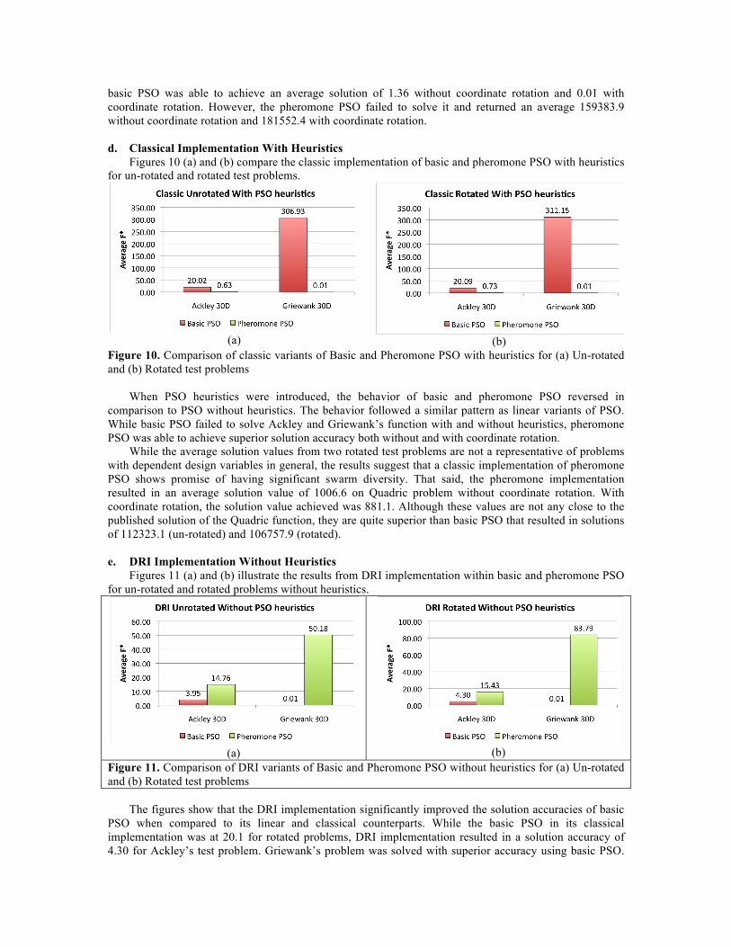
d. Classical Implementation With Heuristics
Figures 10 (a) and (b) compare the classic implementation of basic and pheromone PSO with heuristics for un-rotated and rotated test problems.
(a)
(b)
Figure 10. Comparison of classic variants of Basic and Pheromone PSO with heuristics for (a) Un-rotated and (b) Rotated test problems
When PSO heuristics were introduced, the behavior of basic and pheromone PSO reversed in
comparison to PSO without heuristics. The behavior followed a similar pattern as linear variants of PSO. While basic PSO failed to solve Ackley and Griewank’s function with and without heuristics, pheromone PSO was able to achieve superior solution accuracy both without and with coordinate rotation.
While the average solution values from two rotated test problems are not a representative of problems with dependent design variables in general, the results suggest that a classic implementation of pheromone PSO shows promise of having significant swarm diversity. That said, the pheromone implementation resulted in an average solution value of 1006.6 on Quadric problem without coordinate rotation. With coordinate rotation, the solution value achieved was 881.1. Although these values are not any close to the published solution of the Quadric function, they are quite superior than basic PSO that resulted in solutions of 112323.1 (un-rotated) and 106757.9 (rotated).
e. DRI Implementation Without Heuristics
Figures 11 (a) and (b) illustrate the results from DRI implementation within basic and pheromone PSO for un-rotated and rotated problems without heuristics.
(a)
(b)
Figure 11. Comparison of DRI variants of Basic and Pheromone PSO without heuristics for (a) Un-rotated and (b) Rotated test problems
The figures show that the DRI implementation significantly improved the solution accuracies of basic
PSO when compared to its linear and classical counterparts. While the basic PSO in its classical implementation was at 20.1 for rotated problems, DRI implementation resulted in a solution accuracy of 4.30 for Ackley’s test problem. Griewank’s problem was solved with superior accuracy using basic PSO.
Just similar to the other scenarios, pheromone PSO was unable to solve Ackley and Griewank function. However, the solution accuracies improved by almost 25% on Griewank’s function (67.1 for linear and 50.18 for DRI). Similarly on the classical implementation without heuristics, the solution accuracy improvement was ~89% for DRI implementation. This suggests that the DRI implementation clearly improved the solution characteristics by increasing the swarm diversity within a pheromone PSO. The basic PSO also found similar improvement characteristics.
f. DRI Implementation With Heuristics
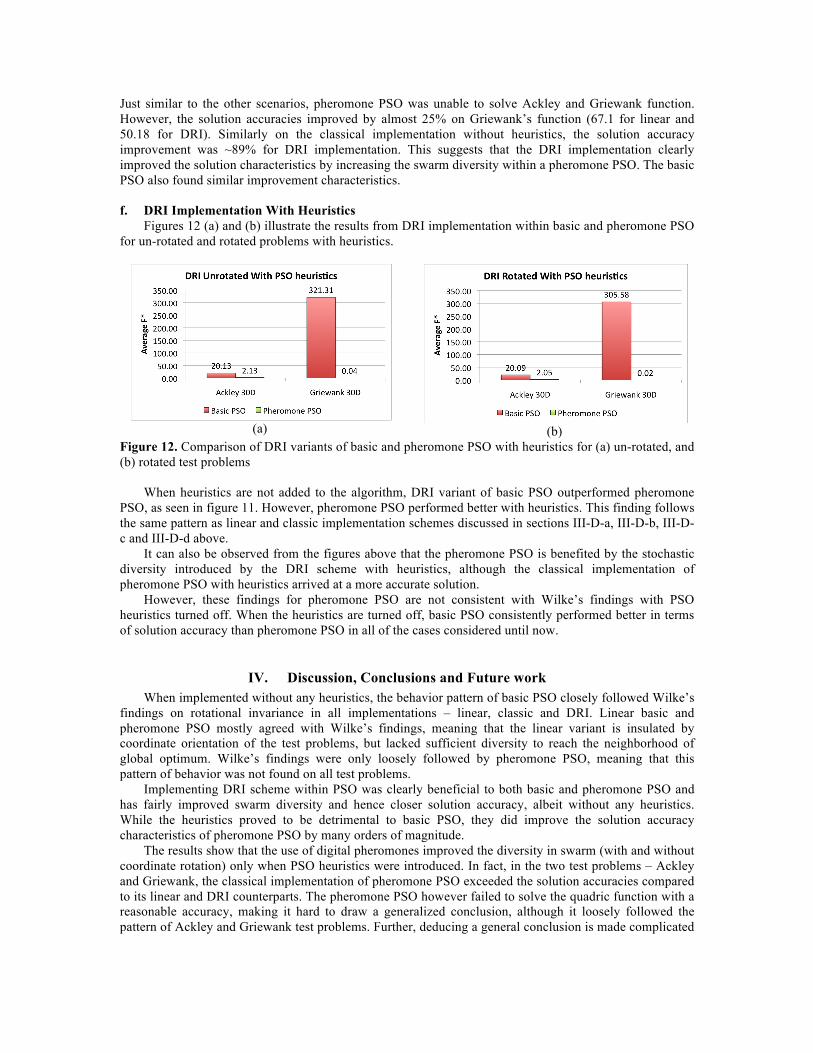
Figures 12 (a) and (b) illustrate the results from DRI implementation within basic and pheromone PSO for un-rotated and rotated problems with heuristics.
(a)
(b)
Figure 12. Comparison of DRI variants of basic and pheromone PSO with heuristics for (a) un-rotated, and (b) rotated test problems
When heuristics are not added to the algorithm, DRI variant of basic PSO outperformed pheromone
PSO, as seen in figure 11. However, pheromone PSO performed better with heuristics. This finding follows the same pattern as linear and classic implementation schemes discussed in sections III-D-a, III-D-b, III-D-c and III-D-d above.
It can also be observed from the figures above that the pheromone PSO is benefited by the stochastic diversity introduced by the DRI scheme with heuristics, although the classical implementation of pheromone PSO with heuristics arrived at a more accurate solution.
However, these findings for pheromone PSO are not consistent with Wilke’s findings with PSO heuristics turned off. When the heuristics are turned off, basic PSO consistently performed better in terms of solution accuracy than pheromone PSO in all of the cases considered until now.
IV. Discussion, Conclusions and Future work When implemented without any heuristics, the behavior pattern of basic PSO closely followed Wilke’s
findings on rotational invariance in all implementations – linear, classic and DRI. Linear basic and pheromone PSO mostly agreed with Wilke’s findings, meaning that the linear variant is insulated by coordinate orientation of the test problems, but lacked sufficient diversity to reach the neighborhood of global optimum. Wilke’s findings were only loosely followed by pheromone PSO, meaning that this pattern of behavior was not found on all test problems.
Implementing DRI scheme within PSO was clearly beneficial to both basic and pheromone PSO and has fairly improved swarm diversity and hence closer solution accuracy, albeit without any heuristics. While the heuristics proved to be detrimental to basic PSO, they did improve the solution accuracy characteristics of pheromone PSO by many orders of magnitude.
The results show that the use of digital pheromones improved the diversity in swarm (with and without coordinate rotation) only when PSO heuristics were introduced. In fact, in the two test problems – Ackley and Griewank, the classical implementation of pheromone PSO exceeded the solution accuracies compared to its linear and DRI counterparts. The pheromone PSO however failed to solve the quadric function with a reasonable accuracy, making it hard to draw a generalized conclusion, although it loosely followed the pattern of Ackley and Griewank test problems. Further, deducing a general conclusion is made complicated
by the fact that basic PSO showed superior performance capabilities only when the heuristics were turned off.
Coordinate rotation result in a new class of test problems than academicians and researchers are typically used to for testing the performance metrics of developed methods. Preliminary results suggest that digital pheromone PSO can address rotational test problems when PSO heuristics are used. The authors could draw a general conclusion that digital pheromones in PSO with the use of heuristics can better address rotational problems than a basic PSO. However, this study used limited number of test problems and further study with more decomposable test problems and with higher dimensions can help make the decision process easier, and hence is a short-term future work for this research.
References
1 Kennedy, J., and Eberhart, R. C., "Particle Swarm Optimization", Proceedings of the 1995 IEEE International Conference on Neural Networks, Vol. 4, Inst. of Electrical and Electronics Engineers, Piscataway, NJ, 1995, pp. 1942-1948.
2 Eberhart, R. C., and Kennedy, J., "A New Optimizer Using Particle Swarm Theory", Proceedings of the Sixth International Symposium on Micro Machine and Human Science, Inst. of Electrical and Electronics Engineers, Piscataway, NJ, 1995, pp. 39-43.
3 Russell C. Eberhart and Yuhui Shi, “Particle swarm optimization: Developments, applications, and resources”, In Proceedings of the 2001 Congress on Evolutionary Computation 2001, 81–86.
4 J.F. Schutte. Particle swarms in sizing and global optimization. Master’s thesis, University of Pretoria, Department of Mechanical Engineering, 2001.
5 A. Carlisle and G. Dozier. An off-the-shelf pso. In Proceedings of the Workshop on Particle Swarm Optimization, 2001, Indianapolis.
6 Vijay Kalivarapu, Jung-Leng Foo, Eliot Winer, “Improving Solution Characteristics of Particle Swarm Optimization Using Digital Pheromones”, Structural and Multidisciplinary Optimization Journal, Springer Publications, ISSN: 1615-147X (Print) 1615-1488 (Online), DOI: 10.1007/s00158-008-0240-9, pp 415 - 427, vol. 37, issue 4, March 2008.
7 Hu X H, Eberhart R C, Shi Y H., “Engineering Optimization with Particle Swarm”, IEEE Swarm Intelligence Symposium, 2003: 53-57.
8 G. Venter and J. Sobieszczanski-Sobieski, “Multidisciplinary optimization of a transport aircraft wing using particle swarm Optimization”, In 9th AIAA/ISSMO Symposium on Multidisciplinary Analysis and Optimization 2002, Atlanta, GA.
9 P.C. Fourie and A.A. Groenwold, “The particle swarm algorithm in topology optimization”, In Proceedings of the Fourth World Congress of Structural and Multidisciplinary Optimization 2001, Dalian, China.
10 Wilke, D. N., Kok, S., Groenwold, A. A., “Comparison of Linear and Classical Velocity Vector Update Rules in Particle Swarm Optimization: Notes on Scale and Frame Invariance”, Int. J. Numer, Meth. Eng., 70:985-1008
11 Shi, Y., Eberhart, R., “A Modified Particle Swarm Optimizer”, Proceedings of the 1998 IEEE International Conference on Evolutionary Computation, pp 69-73, Piscataway, NJ, IEEE Press May 1998
12 Shi, Y., Eberhart, R., “Parameter Selection in Particle Swarm Optimization”, Proceedings of the 1998 Annual Conference on Evolutionary Computation, March 1998
13 Natsuki H, Hitoshi I., “Particle Swarm Optimization with Gaussian Mutation”, Proceedings of IEEE Swarm Intelligence Symposium, Indianapolis, 2003:72-79.
14 Hu, X., Eberhart, R., Shi, Y., “Swarm Intelligence for Permutation Optimization: A Case Study of n-Queens Problem”, IEEE Swarm Intelligence Symposium 2003, Indianapolis, IN, USA.
16 Hu, X., Eberhart, R., “Solving Constrained Nonlinear Optimization Problems with Particle Swarm Optimization”, 6th World Multiconference on Systemics, Cybernetics and Informatics (SCI 2002), Orlando, USA.
17 Schutte, J., Reinbolt, J., Fregly, B., Haftka, R., George, A., “Parallel Global Optimization with the
Particle Swarm Algorithm”, Int. J. Numer. Meth. Engng, 2003. 18 Koh, B, George A. D., Haftka, R. T., Fregly, B., “Parallel Asynchronous Particle Swarm
Optimization”, International Journal For Numerical Methods in Engineering”, International Journal of Numerical Methods in Engineering, 67:578-595, 2006, Published online 31 January 2006 in Wiley InterScience, DOI: 10.1002/nme.1646
19 Hu, X., Eberhart, R., Shi, Y., “Particle Swarm with Extended Memory for Multiobjective Optimization”, Proceedings of 2003 IEEE Swarm Intelligence Symposium, pp 193-197, Indianapolis, IN, USA, April 2003, IEEE Service Center.
20 Tayal, M., Wang, B., “Particle Swarm Optimization for Mixed Discrete, Integer and Continuous Variables”, 10th AIAA/ISSMO Multidisciplinary Analysis and Optimization Conference, Albany, New York, Aug 30-1, 2004.
21 Walter, B., Sannier, A., Reiners, D., Oliver, J., “UAV Swarm Control: Calculating Digital Pheromone Fields with the GPU”, The Interservice/Industry Training, Simulation & Education Conference (I/ITSEC),Volume 2005 (Conference Theme: One Team. One Fight. One Training Future).
22 Gaudiano, P, Shargel, B., Bonabeau, E., Clough, B., “Swarm Intelligence: a New C2 Paradigm with an Application to Control of Swarms of UAVs”, In Proceedings of the 8th International Command and Control Research and Technology Symposium, 2003.
23 Colorni, A., Dorigo, M., Maniezzo, V., “Distributed Optimization by Ant Colonies”, In Proc. Europ. Conf. Artificial Life, Editors: F. Varela and P. Bourgine, Elsevier, Amsterdam, 1991.
24 Dorigo, M., Maniezzo, Colorni, A., “Ant System: Optimization by a Colony of Cooperating Agents”, In IEEE Trans. Systems, Man and Cybernetics, Part B, Vol. 26, Issue 1, pp 29-41, 1996.
25 White, T., Pagurek, B., “Towards Multi-Swarm Problem Solving in Networks”, icmas, p. 333, Third International Conference on Multi Agent Systems (ICMAS’98), 1998.
26 Parunak, H., Purcell M., O’Conell, R., “Digital Pheromones for Autonomous Coordination of Swarming UAV’s”. In Proceedings of First AIAA Unmanned Aerospace Vehicles, Systems, Technologies, and Operations Conference, Norfolk, VA, AIAA, 2002.
27 Vijay K. Kalivarapu, Eliot H. Winer, "Asynchronous Parallelization of Particle Swarm Optimization through Digital Pheromone Sharing", Structural and Multidisciplinary Optimization Journal, Springer Publications, ISSN: 1615-147X (Print) 1615-1488 (Online), DOI: 10.1007/s00158-008-0324-6, pp 263 - 281, vol. 39, issue 3/September, 2009, September 2008.
28 Vijay Kalivarapu, Jung-Leng Foo, Eliot Winer, “Synchronous Parallelization of Particle Swarm Optimization with Digital Pheromones”, Advances in Engineering Software Journal, Vol. 40, Issue 10, pp 975 - 985, DOI: 10.1016/j.advengsoft.2009.04.002, Elsevier publications, April 2009.
29 V. Kalivarapu, E. Winer, “Implementation of Digital Pheromones in PSO Accelerated by Commodity Graphics Hardware”, Proceedings of the 12th AIAA/ISSMO Multidisciplinary Analysis and Optimization Conference, Victoria, British Columbia, Canada, September 2008.
30 V. Kalivarapu, E., Winer, “Digital Pheromone Implementation of PSO with Velocity Vector Accelerated by Commodity Graphics Hardware”, Proceedings of the 50th AIAA/ASME/ASCE/AHS/ASC Structures, Structural Dynamics, and Materials Conference, Palm Springs, California, May 2009.
31 Kalivarapu, V., Winer, E., “A Statistical Analysis of Particle Swarm Optimization With and Without Digital Pheromones”, 48th AIAA/ASME/ASCE/AHS/ASC Structures, Structural Dynamics, and Materials Conference, April 23-26, 2007, Honolulu, HI, AIAA 2007-1882.
32 Salomon, R, “Re-evaluating Genetic Algorithm Performance Under Coordinate Rotation of Benchmark Functions”, BioSystems, vol. 39, pp. 263-278, 1996.
33 Wilke, D. N., Kok, S., Groenwold, A. A., “Comparison of Linear and Classical Velocity Update Rules in Particle Swarm Optimization: Notes on Diversity”, Int. J. Numer. Meth. Engg. 70, pp. 962-984, 2007.
34 Wilke, D. N., Kok, S., Groenwold, A. A., “Comparison of Linear and Classical Velocity Update Rules in Particle Swarm Optimization: Notes on Scale and Frame Invariance”, Int. J. Numer. Meth. Engg. 70, pp. 985-1008, 2007.
35 Liang, J. J., Qin, A. K., Suganthan, P. N., Baskar, S., “Comprehensive Learning Particle Swarm Optimizer for Global Optimization of Multimodal Functions”, IEEE Transactions on Evolutionary Computation, vol. 10, No. 3, pp. 281-295, June 2006.
36 “Orthogonal Matrices”, Web Reference: http://en.wikipedia.org/wiki/Orthogonal_matrix, cited
March 10, 2010. 37 Moler, C., Van Loan C., “Nineteen Dubious Ways to Compute the Exponential of a Matrix, Twenty-
Five Years Later”, SIAM Review, 45:3-49, 2003. 38 Engelbrecht, A., “Fundamentals of Computational Swarm Intelligence, Wiley Publications, NY,
ISBN: 047-009-1916, 2006. 39 “Test Problems in Global Optimization”, Web Reference: http://www-optima.amp.i.kyoto-
u.ac.jp/member/student/hedar/Hedar_files/TestGO_files/Page364.htm, cited March 5, 2010. 40 “GEATbx: Example Functions (Single and Multi-objective Functions) 2 Parametric
Optimization”, Web Reference: http://www.geatbx.com/docu/fcnindex-01.html, Cited March 5, 2010.