BELL-CURVE BASED EVOLUTIONARYOPTIMIZATION ALGORITHM
Jaroslaw Sobieszczanski-Sobieskf', Keith Laba\ and Rex Kincaid*
Abstract
The paper presents an optimization algorithm that fallsin the category of genetic, or evolutionary algorithms.While the bit exchange is the basis of most of the Ge-netic Algorithms (GA) in research and applications inAmerica, some alternatives, also in the category ofevolutionary algorithms, but use a direct, geometricalapproach have gained popularity in Europe and Asia.The Bell-Curve Based Evolutionary Algorithm (BCB)is in this alternative category and is distinguished by theuse of a combination of n-dimensional geometry andthe normal distribution, the bell-curve, in the generationof the offspring. The tool for creating a child is a geo-metrical construct comprising a line connecting twoparents and a weighted point on that line. The pointthat defines the child deviates from the weighted pointin two directions: parallel and orthogonal to the con-necting line, the deviation in each direction obeying aprobabilistic distribution. Tests showed satisfactoryperformance of BCB. The principal advantage of BCBis its controllability via the normal distribution pa-rameters and the geometrical construct variables.
0. Introduction
Vigorous research and increasing applications in opti-mization by Genetic Algorithms (GA) continue becauseof the GA capability to handle discrete problems, mul-tiple minima, and multiple objectives, e.g., Baeck,1997. That list of attractors has recently been extendedto comprise the GA intrinsic concurrent processing ca-pability. This capability is closely aligned with the pre-sent trend in computer technology toward multiproces-sor machines and machine clusters. In addition to its
* Manager, Computational AeroSciences and Multidisci-plinary Research Coordinator NASA Langley ResearchCenter, MS 139 Hampton VA 23681, AIAA Fellowf Research Assistant, College of William and Mary* Professor, College of William and Mary
Copyright @ 1998 by the American Institute ofAeronautics and Astronautics, Inc. No copyright isasserted in the United States under Title 17,U.S. Code.The U.S. Government has a royalty-free license toexercise all rights under the copyright claimed herein forGovernmental Purposes. All other rights are reserved bythe copyright owner.
utilitarian values, the GA has been seen as an eleganttransposition of the biological mechanism of "the sur-vival of the fittest" onto the grounds of engineering.
While the original, biology-inspired GA that employscrossover and random mutations, and operates on 0-1bits in binary strings as analogs of genes and chromo-somes, remains the mainstay of research and applica-tions in America, an alternative approach, also in thecategory of evolutionary optimization, has been gainingpopularity in Europe and Asia. This approach calls forchanging design variables by direct applications of therules of probability without operating on binary strings.
Once the confines of the biology emulation are dis-carded, the ways one can generate successive genera-tions is limited only by the imagination. This has re-sulted in a gamut of techniques varying in ingenuityand complexity. An example of a very simple mecha-nism is found in Grill and Hartmann, 1998. It altersdesign variables by adding to each an increment whosemagnitude is governed by the familiar "bell-curve"probability distribution and generates a child from asingle parent (asexual reproduction). A contrastingexample of a more complex technique is the algorithmproposed in Ono and Kobayashi, 1997. Their techniqueconnects two parents by a line in the design space andplaces the child away from that line at a distance con-trolled by the location of a third parent.
An advantage that motivated the development of tech-niques such as the two above examples is, primarily, animproved controllability of the entire optimizationprocess. In addition, premature convergence caused bya loss of diversity in the successive generations(population stagnation) that often occurs in the original,biology-inspired GA is remedied. Another motivationis the natural human desire to improve on the devicesoriginally inspired by the natural world.
In this paper, we report on a technique in the samecategory as that of Ono and Kobayashi, 1997. It alsouses two parents connected by a line in the design spaceas a basis for generation of children. However, insteadof using a third parent, it relies throughout on the fa-miliar, "bell-curve" probability distribution. A variantof the technique selects one parent by the objectivefunction criterion, and the other by the degree of satis-faction of the constraints. Testing in structural applica-tions demonstrates the technique's effectiveness in lo-cating constrained minima in a rather complex design
2083American Institute of Aeronautics and Astronautics
space, and its ease of controllability, achieved withoutsacrificing the valuable concept of inheritance fromtwo-parents (the concept abandoned in the asexual re-production) .
1. Notation
B - point where orthogonal subspace intersects LC-chi ldofPl&P2D - distance between PI, and P2 on Lf j , f2 - fitness measures of parents PI and P2F(X) - objective function.FP - F with a penalty term added for a constraint viola-tion<g> - vector of NGV violated constraintsg(X) - vector of NG inequality constraint functionsL - line from Parent 1 through Parent 2, from - to + in-finityM - point on L, the origin of coordinate sN(m, a) - normal distribution with mean m and vari-ance CT; a code to generate this may be found in Pritsker1986.NP - number on individuals in a generationNX - number of the design variables, length of X.p - penalty factorPI, P2 - pair of parent pointsr - coefficient used to define a in the N-distribution ofRR - radius of hypersphere in NX-1 subspace, centeredon point Bs - coordinate originating at M, positive toward P2.W - structural weight (or volume)X - vector of NX design variables.XI, X2, XB, Xc, and XM - X vectors associated with PI,P2, B, C, and M.o - standard deviation
2. The Bell Curve-Based (BCB) Algorithm
The BCB algorithm solves the optimization problem
FindMinimizeSatisfy
XF(X)g(X)<=0
where X, F(X) and g(X) may be continuous or discrete.In simplest terms, the BCB algorithm creates a childfrom two parents who are selected out of NP individu-als in the current generation in the same way as in theoriginal GA. The selection fitness criterion penalizesconstraint violations by adding a penalty term to F
In the BCB variant (BCB/V), Parent 1 is selected by Fand Parent 2 by max(<g>).
The crux of the BCB Algorithm is the way a child iscreated from parents by the following geometrical con-struct. The paired parents, PI and P2 in Figure 1, areconnected by line L in the NX-dimensional designspace. They are a distance D apart. Point M is placedon L between the parents at a location that deviatesfrom the mid-point toward the parent of better fitness.Coordinate s, originating at M and pointed toward Par-ent 2, is used to locate point B on L by a random prob-ability distribution, the bell-curve from which the algo-rithm takes its name:
3) SB = N(0, a)
where N(0, a) is a normally distributed random numberwith mean 0 and standard deviation a given in units ofD.
Now, we define a subspace orthogonal to L and inter-secting L at B. The orthogonality reduces the subspacedimensions to NX-1. In that subspace we create a hy-persphere of radius R whose length is again governedby the positive side of the normal distribution in unitsof(rD)
4) R=IN(0,
2) = F + p£max(<g>);
Finally, point C representing the child is placed on thesurface of the hypersphere using a uniform, not normal.distribution over that surface. Owing to the subspaceorthogonality to L, the chance of the child falling backon either parent is exceedingly small.
Figure 1 shows a three-dimensional design space, inwhich the hypersphere reduces to a circle of radius R,perpendicular to L at B, and point C may fall anywhereon the perimeter of that circle with equal probability.
In the remainder of BCB one may again use any of thestandard GA techniques. In the study reported herein,one repeats the parent selection and the child generationprocess until the number of children reaches NP. Thechildren are added to the parents resulting in a popula-tion that swells to 2 NP. Selection based upon the ap-plication of the Fp fitness criterion to all the individuals,young and old alike, reduces the population back to NP,and the process starts over - see Appendix for the BCB& BCB/V step-by-step recipe and further details.
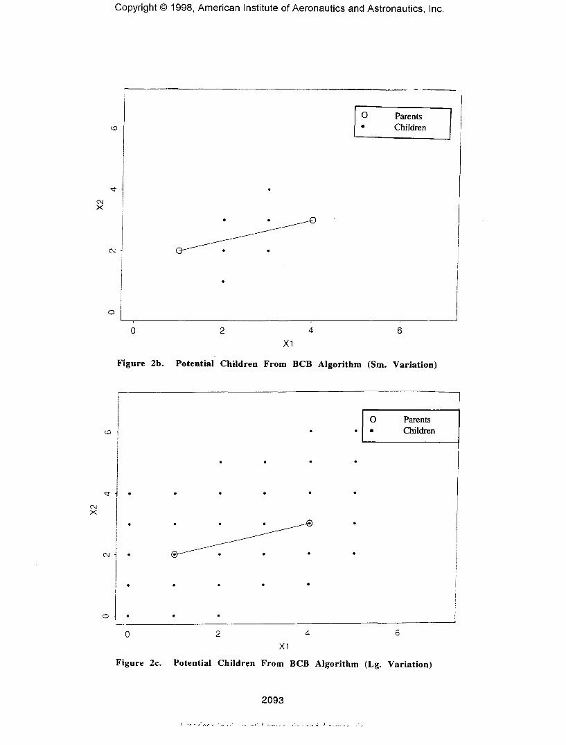
The way BCB algorithm generates children contrastswith that of the original GA (O/GA) as shown in Figure2 for a case of integer variables in a 2D space. Wheninteger variables are represented as a binary string,there is a limited number of ways these strings may be
2084American Institute of Aeronautics and Astronautics
mixed by the O/GA crossover mechanism. Figure 2aillustrates the consequences, demonstrating the cluster-ing of the O/GA children toward the parents. Intrigu-ingly, this clustering seems to reflect the folk wisdomthat among siblings, one child "takes after the mother"and the other "takes after the father", rather than bothreflecting features of the parents evenly mixed. Notethat the children from random mutations (each mutationchanges one 0 to 1 or vice versa) also fall in that clus-tering pattern. It has also been observed, e.g., Ono andKobayashi, 1997, that the degree of feature inheritanceis affected by the angles formed by L and the coordi-nate axis. Furthermore, that inheritance also dependson the choice of the numerical system, binary or deci-mal.
Figs. 2b and c depict the BCB children for a small and alarge a. Comparing to Figure 2a, their distribution ismore centered on the line connecting the parents, sothat most of the children inherit, mix, and average thefeatures of the parents (within a restriction imposed byinteger nature of the variables). In this regard, the BCBimproves on both O/GA, and on the asexual reproduc-tion that abandons the two-parent inheritance. Observe,also, that the normal distribution allows some of thechildren to fall beyond the parents as measured alongthe coordinate axis and along L. The tails of the bell-curve enable them to fall anywhere within the designspace limits so that additional random mutations maynot be necessary to maintain the population diversity.Also, it is apparent that owing to the use of the localvariable s and the normal distribution, the locations ofthe children do not depend on the orientation of L andon the choice of the numerical system.
To recapitulate this narrative description of the BCBalgorithm, the algorithm may be controlled by:
• lower bound on the inter-parent distance D to keep theparents far enough apart to foster diversity• standard deviation a; two different as are used tocontrol the location of B and the length of R (equations3 and 4).• penalty coefficient p• choosing between BCB and BCB/V
In addition, the usual GA controls apply to the parentselection and formation of the next generation from theparents and their children.
3. Testing and Results
One of the examples is depicted in Figure 3. It is a hubstructure which appears also in Balling and Sobi-eszczanski-Sobieski, 1994. Each member of the hub isan I-beam rigidly attached to the hub and to the wall.The structure is optimized for minimum weight
(equivalent to volume for the homogeneous materialused), so that the smaller the fitness the better thestructure.
The beam cross-sectional dimensions are the designvariables, and the constraint functions reflect the mate-rial allowable stress and the overall and local buckling.Additional constraints are also imposed on the hub dis-placements. The top and bottom flanges of the I-beamare not of the same dimensions, hence the cross-sectionof each I-beam requires 6 design variables. Details aregiven in the Appendix, including the constraint functionformulations; they may also be found in Padula, et. al.,1997.
Utility of the hub structure as an optimization test casestems from its ability to be enlarged by adding as manymembers as desired without increasing the dimension-ality of the load-deflection equations. These remain3x3 equations for a 2D hub structure regardless of thenumber of members. While analytically simple, thehub structure design space is complex because thestress, displacement, and buckling constraints are richin nonlinearities and couplings among the design vari-ables.
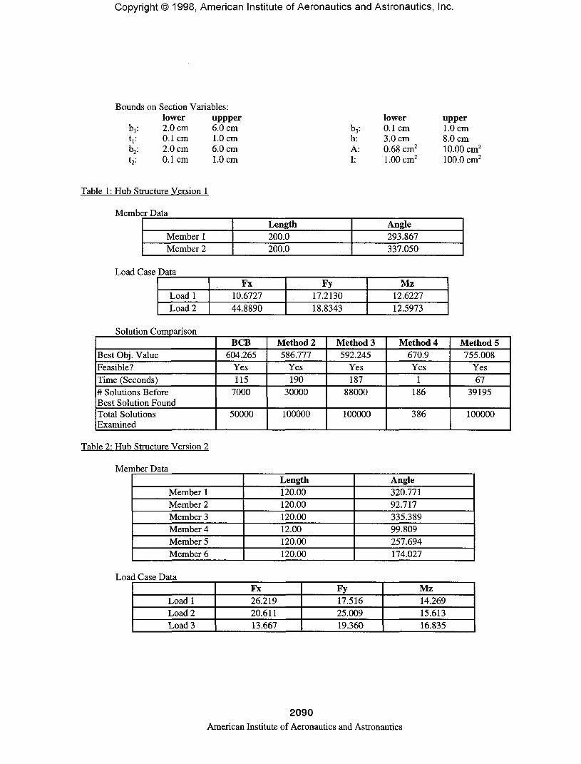
The results included herein are for two versions of thehub structure: Version 1 comprising 2 members, andloaded by 2 loading cases; Version 2 is made up of 6members, and loaded by 3 loading cases. In both ver-sions the members have the same type of I-cross-section defined by 6 design variables.
To validate the GA results and to provide a comparison,a few other methods were exercised:
• Method 2: a crossover method where the child's val-ues are taken directly from one parent or the other. Abasic mutation is applied that adds or subtracts a uni-form random variable on the range of zero to 1/10 ofthe range of allowable values for that particular vari-able.
• Method 3: a crossover method where the child's val-ues are calculated as a direct average of the two corre-sponding parent values. The mutation is the same as inmethod 2.
• Method 4: a usable-feasible search algorithm(Vanderplaats 1973)
• Method 5: random generation of 10000 solutions toshow that the genetic algorithms produce results betterthan a random examination of the solution space.
BCB and methods 2-5 were executed for Version 1;Version 2 was optimized using BCB, methods 4 & 5,and by BCB/V.
2085
American Institute of Aeronautics and Astronautics
Table 1 and 2 define the structure for Versions 1 and 2and show the corresponding results. Note that Version2 in Table 2 has one member much shorter than othersto create a case whose solution is known in advance.That is, all members other than the short one shouldshrink to minimum gage dimensions. Both Method 4and BCB confirmed that. Table 2.1 shows results forVersion 2 with varied member length. Comparison ofthe BCB and BCB/V performances is presented in Ta-ble 3.
To test the BCB ability to locate the global minimum, asingle member hub structure test was devised, shown inFigure 4. In that test the load is limited to Fx only andthe member is optimized by adding to the 6 cross-sectional design variables the orientation angle relativeto the loading force, as the 7th variable. Zero angle cor-responds to pure compression. The global minimum isexpected at the angle 180 degrees in pure tension, thesecond minimum is known to occur at 0 degrees incompression, separated by the maximum weight atabout 90 degrees in bending. The convergence of BCBon the optimal angle is demonstrated in Table 4.
The number of individuals in a population was 10 in allthe tests reported herein. This relatively small numberwas found experimentally to be sufficient in these tests.
A typical BCB histogram is in Figure 5. The dottedline represents the best objective (structural weight)fitness in the generation, and the solid line depicts thepenalty function Fp. The places where the two lines donot overlap indicate designs where the most fit memberis infeasible. In this case, the fitness value is based onthe structural weight plus the penalty term, resulting inthe discrepancy in the two values. It is apparent thatBCB selected feasible designs from the initial popula-tion and maintained that feasibility throughout. To doso, BCB had to be supplied with a judiciously chosenvalue of p.
Controllability of BCB is demonstrated in Figure 6. Itshows how the value of a (eq. 3) that governs the lo-cation of B makes the process converge faster. On theother hand, a larger value of a enables one to "cast awider net" for more diverse designs at the penalty ofconverging slower. The coefficient r that governs R (ie.a in eq.4) has a similar effect as illustrated in Figure 7.
Examination of a large number of designs generated inthe BCB process revealed that, typically, a group offeasible and near optimal designs results from the proc-ess.
4. Conclusions
An algorithm was developed in the class of evolution-ary optimization for creating design populations thatimprove in a series of successive generations. Distin-guishing features of the Bell-Curve Based (BCB) algo-rithm are the use of a new geometrical construct in thedesign space, combined with the probability calculustools of the uniform and normal distributions (bell-curve) for deriving children designs from the parentdesigns that are paired by a fitness criterion of the ob-jective function penalized for any violation of the con-straints. This mechanism replaces the classical, biol-ogy-inspired, bit-exchange (crossover) as a means bywhich to pass the parent features to the children. In avariant of the algorithm (BCB/V), one parent is quali-fied by the value of the objective, the other by the valueof the maximum violated constraint.
BCB and BCB/V have been tested on a number of casesand both performed as intended in all of them. A sam-ple test reported herein was a minimum weight(volume) design of a redundant structure with up to 36cross-section variables. To create a case of multiplelocal minima, the member orientation angle was also adesign variable in one of the tests. The strength, localbuckling, and displacement limitations generated 36highly nonlinear constraints. In these tests the algo-rithm was able to do as well or better than a benchmarkNLP search algorithm in terms of the objective functionvalue and the ability to eliminate constraint violations.Regarding the number of function evaluations it was onpar with other GAs and, as expected, not competitivewith gradient-guided NLP techniques. However, supe-rior to the NLP techniques, the algorithm is not ham-pered by discrete variables, and its capability to findglobal minima in presence of local minima was demon-strated in the test.The principal motivation for development of BCB wasto have the adaptability and flexibility needed to pre-vent premature convergence that occurs in many GAprocesses because of the loss of population diversity.Indeed, owing to the intrinsic controllability of thenormal distribution by the mean and variance parame-ters, combined with the malleability of the geometricalconstruct, BCB has exhibited the desired adaptabilityand flexibility in the tests. Another merit of BCB is itsability to identify a number of feasible and near-optimalsolutions, as opposed to a point solution typical for anNLP technique.
Future work is aimed at furthering BCB's adaptabilityto the peculiarities of the design space topology, incor-poration of the gradient data wherever available, and onthe elapsed time reduction by the use of concurrentprocessing for simultaneous generation of individualdesigns.
2086
American Institute of Aeronautics and Astronautics
Baeck, T., (ed.): Proceedings of the 7th InternationalConference on Genetic Algorithms; Michigan StateUniversity, East Lansing, MI, July 19-23, 1997; Mor-gan Kaufmann Publ., San Francisco, 1997.
Balling, R.J.; and Sobieszczanski-Sobieski, J.: An Al-gorithm for Solving the System-Level Problem in Mul-tilevel Optimization; ICASE Report No. 94-96, NASAContractor Report 195015; NASA Langley ResearchCenter; Institute for Computer Applications in Scienceand Engineering, Hampton VA 23681; December 1994.
Grill, H.; and Hartmann, D.: Mixed-Discrete StructuralOptimization with Distributed Advanced EvolutionStrategies. Proceedings of the Australasian Conferenceon Structural Optimisation, Feb. 11-13, 1998, Sydney,Australia; Oxbridge Press Publ. Highpoint, Victoria,Australia; pp. 79-86.
Ono, I; and Kobayashi, S.: A Real-coded GA for Func-tion Optimization Using Unimodal Normal DistributionCross-Over. Proceedings of the 7th International Con-ference on Genetic Algorithms; Michigan State Univer-sity, East Lansing, MI, July 19-23, 1997; MorganKaufmann Publ., San Francisco, 1997. Baeck, T., (ed.).pp. 246-253.
Vanderplaats, G.N.: CONMIN - A FORTRAN Programfor Constrained Function Minimization; NASA TM X-62282, August 1973.
Pritsker, A. Alan B.: Introduction to Simulation andSLAM IIHalsted Press, John Wiley & Sons, New York 1986
Knuth Donald E.: The Art of Computer Programming;Addison-Wesley Reading, Massachusetts 1969
Padula, S.L., Alexandrov, N., and Green, L.L..: MDOTest Suite at NASA Langley Research Center. Pro-ceedings of the 6th AIAA/NASA/ISSMO Symposiumon Multidisciplinary Analysis and Optimization;Bellvue, WA, September 4-6, 1996; American Instituteof Aeronautics and Astronautics, 1996. pp. 410-420.Accessible as a website:http://fmad-www.larc.nasa.gov/mdob/
Appendix
1) Step-by-step recipe andmathematical details;
2) Orthogonal hypersphere; and3) Test Case details
I) The algorithm's step-by-step recipe isas follows (BCB/V notes the only stepswhere BCB/V differs):
1) Generate a population of designs by anytechnique commonly used in a conventionalGA.
2) Analyze each design for the value of theobjective function and constraints, eq. 2. Foreach design generate a single "measure of fit-ness" combining the value of the objective (thesmaller the better) and of the constraints(negative = satisfied, zero = active (critical),positive = violated); thus, a smaller fitness re-flects a better design.
In BCB/V, place individuals from N in twopopulations of N each, rank one by F and theother by max(g).
3) Pair-up the designs to form parents formating, rewarding fitness (as measured by Fp)with more chances to mate. The effect is thatindividuals that are more fit participate inmore parent pairs, and end up contributingtheir characteristics to more childr^. BCBuses the electronic roulette to do this, as in theconventional GA.
In BCB/V, one parent is selected from thepopulation ranked by F, the other from the oneranked by max(<g>).4) Generate a child:
• Consider a design space in n-dimensions. Figure 1 illustrates a 3Dexample. Design points PI and P2 arethe parents, assignment of the PI andP2 labels is arbitrary. The hyperline Lconnects the parents. The prefix"hyper" reminds us that we are deal-ing with n-dimensional space ofwhich 3D simplification is depictedin Figure 1. Line L extends beyondPI and P2 to infinity, emphatically, itis not merely a (P1.P2) segment. PIand P2 define vectors XI and X2.The distance D between PI and P2 is
D = X22)1/
Coordinates XM of point M on L be-tween PI and P2 are
XM = X2 + (XI - X2) k
2087American Institute of Aeronautics and Astronautics
(recall, a smaller fitness is better, thusas f2 improves relative to f,, k will de-crease, moving point M closer to X2and vice versa)
. The variate, NB, is generated relativetoXM
NB = N(0,a);
Or, equivalently, relative to X2
NB = N(XM,a)
• Assume a is in the units of D andplace point B at a distance from Mmeasured by SB from eq.3
XB = XM + (X2-Xl)N(0,a)/D;
or use the equivalent formula
XB = X2 + (XI - X2) N(XM, a)/D;
• Generate an N-dimensional hyper-sphere with radius R that is orthogo-nal to L at B, and place child C on thesurface of the above hypersphere,using a uniform probability distribu-tion over that surface, i.e., each pointon the surface has the same chance ofselection (details in Appendix, Sec-tion 2)
• Xc defines the child design point. Ifany element of Xc exceeds its boundsit is reset to that bound
5) Repeat #3 to 5 to produce the entire off-spring generation6) Group together the newly generated chil-dren population and the previous populationfrom which their parents were drawn (thegrouped population comprises 2 NP individu-als) and select the most fit individuals. Theseindividuals represent the next generation. Thesize of the next generation is kept at NP bydiscarding the least fit half in each successivegrouped population. Then, repeat from #2until termination criteria are met.
2) Child C Placement on Hypersphere that is Orthogo-nal to L and has N-distributed R
1) Shift the coordinate system X origin to B.
2) Rotate X so that X] coincides with L point-ing from PI to P2.3) Apply algorithm by Knuth 1969:• Set and maintain X! = 0• Let X2, X3, ... Xn.ibe normal variates dis-
tributed as N(0,l).• Letb = (X2
2 + X32+.. . + Xn.,2)1/2
• Generate radius R distributed as the posi-tive half of N(0, (r D)) for assumed C
• Generate point C whose coordinates are
Xc = {0, (R*X2) / b, (R * X2) / b,
3) Test Case Details
The solution method is the standard, linear, displace-ment-based finite element method, using the beam ele-ment in a slender beam formulation that neglect thetransverse shear stress deformations and preserves theKirchoff's assumption of the beam cross-sections re-maining planar under the load. The structure is two-dimensional for analysis purposes, with the exceptionof out-of-plane member buckling. The following de-fines the constraints.
Displacement Constraints at the hub:
d/da - 1 < 0 q/qa - 1 < 0
d = resultant translational displacementq = rotational displacement
two-member hub:six-member hub:
qa0.2cm0.2cm
1.0 rad1.0 rad
Stress Constraints:
Normal and shear stresses (s and t) wereevaluated within the cross section at the topand bottom extreme fibers, at the centroid, andat the top and bottom of the web. This wasdone at both ends of the member except for thecentroidal stresses which are constant alongthe length of the member. The following stressconstraint was imposed at each location:
s e q / s a - l<0
Se, = von Mises-Huber equivalent stress =(s2 + 3t2)"2
sa = allowable stress = 25 kN/cm2
In-Plane Buckling Constraint for each beam:
2088American Institute of Aeronautics and Astronautics