1

ØAMET2200Business Decision Making Using Data

Lecture 10

Instructor: Fenella Carpena

November 8, 2019

2

Announcements

I Problem Set 4 has been posted. Due Nov. 21 at 11:59 PM.

I Lecture and Office Hours (OH) next week are cancelled

I No lecture on Nov. 15

I No OH on Nov. 11

I Last meeting for this course is Nov. 22

I Course Wrap Up

I Practice Mini-Final Exam

I Extra OH schedule

I Nov. 18 (Monday) 4-5PM

I Nov. 25 (Monday) 4-5PM

I Nov. 29 (Friday) 10-11AM

I Dec. 2 (Monday) 4-5PM

I Dec. 3 (Tuesday) 4-5PM

3

Part 4 of this Course: Building regression models

I You want to build a model to predict outcomes from data youhave

I What’s the best model you can build?

I Today: Modeling time series for forecasting into the future

4

Agenda for Today

I Smoothing Time Series Data

I Regression Models for Time Series

I Polynomial Trends

I Autoregressions

I Checking Regression Conditions

I Chapter 27

5

Time Series

I A time series is a sequence of data points ordered in time

I Example: daily price of Apple stock, annual inflation rate

I A time series consists of three components:

yt = Trendt + Seasonalt︸ ︷︷ ︸pattern

+ Irregulart︸ ︷︷ ︸random

I Trend: smooth, slowly meandering pattern

I Seasonal: cyclical oscillations related to seasons

I Example: Sales of skis are lower after winter

I When we forecast a time series, we are extrapolating the trendor seasonal component

I The irregular variation affects how accurate our forecasts are

6

Time Series

I Sometimes the time series data we have are “smoothed out”

I Smoothing means removing irregular and seasonalcomponents to enhance the visibility of a trend

I In other words, removing short-term fluctuations andhighlighting longer-term trends

I We’ll briefly discuss three ways of smoothing

1. Simple Moving Average

2. Exponentially-Weighted Moving Average

3. Seasonal Adjustment

I Often seen in finance (stock trading) and macroeconomicapplications

7

1. Simple Moving Average

I The 5-period Simple Moving Average (SMA) is theunweighted average of the 5 most recent data points prior toand including the current period

SMAt,5 =Yt + Yt−1 + Yt−2 + Yt−3 + Yt−4

5

I How does it work in practice? Example:

8

1. Simple Moving Average

I Note that we can also calculate the SMA for any number ofperiods (other than 5)

I The more terms that are averaged, the smoother the estimateof the trend

9

2. Exponentially-Weighted Moving Average (EWMA)

I EWMA is a weighted average of past observations withgeometrically declining weights

I More recent values of Y receive more weight than thosefurther in the past

I Can be written St = (1−w)Yt + wSt−1, where w is a weight

I The current smoothed value is the weighted average of thecurrent data point and the prior smoothed value

I The choice of w affects the level of smoothing

I ↑ w =⇒ smoother St

I ↑ w =⇒ St trailing more behind the observations

I How to pick w? Depends on the application

I In finance, it is common to pick a number of days N and setw = (N − 1)/(N + 1)

10

2. Exponentially-Weighted Moving Average (EWMA)

I Larger N (higher w): time series is smoother

I Larger N (higher w): trailing more behind the observations

11

Comparison of SMA and EWMA

I EWMA reacts quicker to price changes than SMA

I EWMA is more “sensitive” than SMA

12

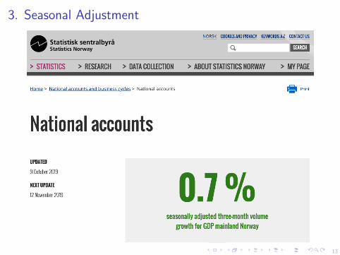
3. Seasonal Adjustment

I Seasonal adjustment means removing the seasonal componentof a time series

I The difference between the observed time series and theseasonally adjusted time series is the seasonal component

I Many government-reported time series are seasonally adjusted

I For example:

I bruttonasjonalprodukt or Gross Domestic Product (GDP)

I See https://www.ssb.no/en/

nasjonalregnskap-og-konjunkturer/statistikker/knr

Why seasonally adjust these statistics?

Because of climatic conditions, public holidaysand holidays in July and December, the intensity of theproduction varies throughout the year. The same appliesto household consumption and other parts of the economy.

13

3. Seasonal Adjustment

14

3. Seasonal Adjustment

15

Case Study for Today: Forecasting Unemployment Rate

I The unemployment rate (the percentage of the labor forcethat is unemployed) is one of the most watchedmacroeconomic variables

I Many government agencies track the unemployment rate

I If the unemployment rate is high, there will be greater demandfor government services (e.g., at NAV)

I Businesses also watch the unemployment rate

I If the unemployment rate is decreasing, managers worry thatthere will be pressure to raise wages, cutting into profits

I Suppose that you are an economist at Norges Bank, and yourjob is to develop statistical models for the unemployment rate

16

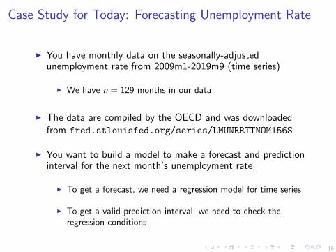
Case Study for Today: Forecasting Unemployment Rate

I You have monthly data on the seasonally-adjustedunemployment rate from 2009m1-2019m9 (time series)

I We have n = 129 months in our data

I The data are compiled by the OECD and was downloadedfrom fred.stlouisfed.org/series/LMUNRRTTNOM156S

I You want to build a model to make a forecast and predictioninterval for the next month’s unemployment rate

I To get a forecast, we need a regression model for time series

I To get a valid prediction interval, we need to check theregression conditions

17

Case Study for Today: Forecasting Unemployment Rate

18

Case Study for Today: Forecasting Unemployment Rate

When analyzing a time series, always begin with a time plot!

19

Regression Models for Time Series

I We can use regression models to generate forecasts for timeseries data

I We’ll discuss two types of explanatory variables that we canput in our regression model for forecasting

1. The time index t: polynomial trend

2. Prior values of the response variable y : autoregression

I Regression with time series data require the same assumptionsas in the MRM

I The most important one is usually the independence of errors

20

Polynomial Trends

I A regression model for a time series that uses powers of t asexplanatory variables

I Example: a third-degree or cubic polynomial

unempratet = β0 + β1t + β2t2 + β3t

3 + εt

I Note that we can also have powers other than three (e.g.,sixth-degree polynomial)

I Why do we care? Polynomials helps to better capturecurvature in the data

21

Case Study: Linear Fit

unempratet = β0 + β1t + ε

22

Case Study: Polynomial Trends

I The simple regression of unemprate on t (without polynomialterms) clearly does not give us a good fit

I We can try a fifth-degree polynomial

unempratet = β0 + β1t + β2t2 + β3t

3 + β4t4 + β5t

5 + εt

23

Case Study: Polynomial Trends

24

Case Study: Polynomial Trends

unempratet = β0 + β1t + β2t2 + β3t

3 + β4t4 + β5t

5 + εt

25

Case Study: How to use polynomial trends?

I How do we make forecasts using the regression withpolynomial trends?

I Plug in the time period in the variable t

I Example: Using the fifth-degree polynomial trend model,what is the forecast and prediction interval of theunemployment rate in November 2019?

26

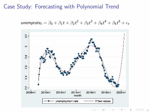
Problems with Polynomial Trends

I Be cautious when using polynomial trend to forecast time series

I Polynomials extrapolate past trendsand lead to poor forecasts when trends change direction

I Forecasting with polynomial is useful only if the patternspersist into the future

I You cannot rely on a polynomial that fits well during the stableperiod if you suspect that the stability may be short-lived

I Polynomials with high powers of time can be very unreliable

I They will fit historical data,but not necessarily generate accurate forecasts

I Relates to “overfitting”

27

Case Study: Forecasting with Polynomial Trend

unempratet = β0 + β1t + β2t2 + β3t

3 + β4t4 + β5t

5 + εt

28

Autoregressions

I An autoregression is a regression that uses prior values of theresponse as predictors

I These prior values are called lagged variables

I The simplest autoregression has one lag called a first-orderautoregression, AR(1)

yt = β0 + β1yt−1 + εt

I We can also have more lags than one

I Example: third-order autoregression, AR(3)

yt = β0 + β1yt−1 + β2yt−2 + β3yt−3 + εt

29

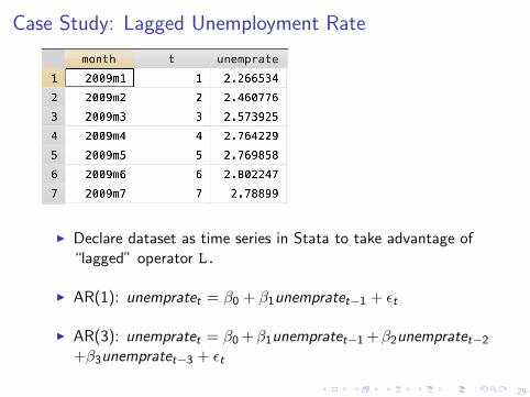
Case Study: Lagged Unemployment Rate

I Declare dataset as time series in Stata to take advantage of“lagged” operator L.

I AR(1): unempratet = β0 + β1unempratet−1 + εt

I AR(3): unempratet = β0 +β1unempratet−1 +β2unempratet−2

+β3unempratet−3 + εt

30

Case Study: AR(1) for Unemployment Rate

Even with just 1 explanatory variable, this regression explains morevariation in unemployment rate than the fifth-order polynomial

31

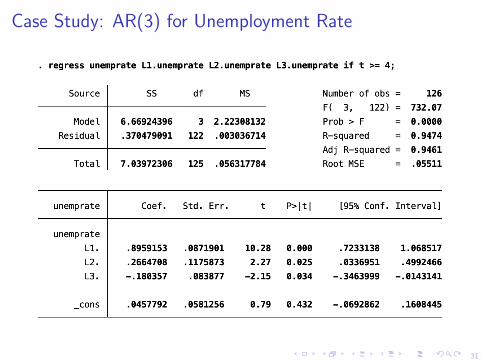
Case Study: AR(3) for Unemployment Rate

32

Understanding and Building Autoregressions

I The slopes in autoregressions are not easily interpretable

I Autoregressions are generally used for short-term forecasting

I Not for analyzing how explanatory variables impact y

I How many lags to include? Usually done by trial and error

I Try different lags, select the model that offers the best

combination of goodness of fit (R2

and se) and statisticallysignificant coefficients

I Case study example: AR(3) has almost the same R2

asAR(1), so we pick AR(1) model for simplicity.

I Why do we care about autoregressions?

I Lets us capture large amounts of dependence in the y variable

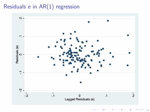
I Helps to ensure that independence of residuals holds

33

Residuals e in fifth-order polynomial regression

corr(e, et−1) = 0.7209

Durbin Watson (DW) statistic = 0.5496

34

Residuals e in AR(1) regression

35

Case Study: Forecasting unemployment with AR(1) Model

I What is the forecast for Oct. 2019 (1 period beyond data)?

I What is the 95% prediction interval for this forecast?

36

Case Study: Forecasting unemployment with AR(1) Model

I What is the forecast for Nov. 2019 (2 periods beyond data)?

I Prediction interval for Nov. 2019 is hard to compute by hand(not covered in this course)

I Forecasts are used in place of observations

I Uncertainty is compounding

37

Checking the Model

I As before, we need to check the multiple regression conditions

1. Linear

2. No obvious lurking variables

3. Errors are independent

4. Errors have similar variances

5. Errors are nearly normal

I The most important of these in time series context is theindependence of the model errors

I Usually the residual et is correlated with et−1

I If the errors are not independent, se and standard error of theslopes are too small

I Use Durbin-Watson statistic to check dependence

I Can’t apply DW test when using an autoregression

38

Independent vs. Dependent Residuals

39

Summary and Best Practices

I Examine these plots of residuals when fitting a time seriesregression

I Time plot of residuals

I Scatter plot of residuals vs. fitted values

I Scatter plot of residuals versus lags of the residuals

I The above plots can show dependence in the residuals

I Using autoregressions can help deal with dependence

I Avoid polynomials with high powers