AMG for a Peta-scale Navier Stokes Code

James Lottes

Argonne National Laboratory

October 18, 2007

The Challenge

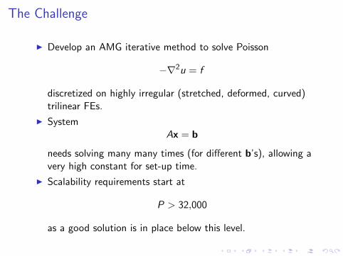
I Develop an AMG iterative method to solve Poisson

−∇2u = f

discretized on highly irregular (stretched, deformed, curved)trilinear FEs.

I SystemAx = b

needs solving many many times (for different b’s), allowing avery high constant for set-up time.

I Scalability requirements start at

P > 32,000

as a good solution is in place below this level.

Outline

I Notation for iterative solvers and multigrid (3 slides)

I Analysis of two-level multigrid, illustrated on model problem

I AMG iteration design

Iterative Solvers

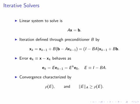
I Linear system to solve is

Ax = b.

I Iteration defined through preconditioner B by

xk = xk−1 + B(b− Axk−1) = (I − BA)xk−1 + Bb.

I Error ek ≡ x− xk behaves as

ek = Eek−1 = E ke0, E ≡ I − BA.

I Convergence characterized by

ρ(E ), and ‖E‖A ≥ ρ(E ).

Multigrid Iteration

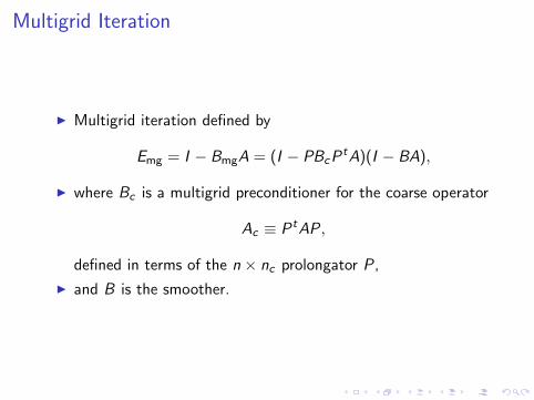
I Multigrid iteration defined by

Emg = I − BmgA = (I − PBcPtA)(I − BA),

I where Bc is a multigrid preconditioner for the coarse operator

Ac ≡ PtAP,

defined in terms of the n × nc prolongator P,

I and B is the smoother.

C-F Point Algebraic Multigrid

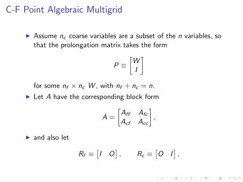
I Assume nc coarse variables are a subset of the n variables, sothat the prolongation matrix takes the form

P ≡[WI

]for some nf × nc W , with nf + nc = n.

I Let A have the corresponding block form

A =

[Aff Afc

Acf Acc

],

I and also let

Rf ≡[I O

], Rc ≡

[O I

].

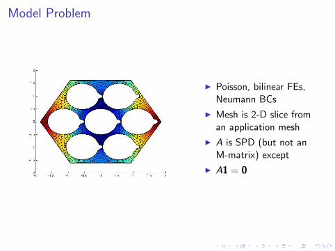
Model Problem

I Poisson, bilinear FEs,Neumann BCs

I Mesh is 2-D slice froman application mesh

I A is SPD (but not anM-matrix) except

I A1 = 0

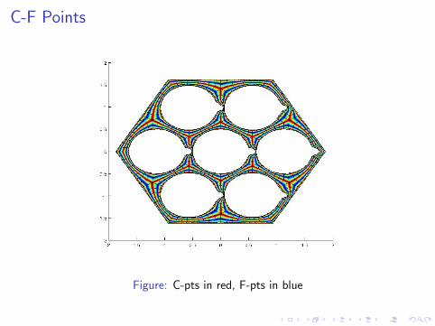
C-F Points

Figure: C-pts in red, F-pts in blue

Prolongation

The energy-minimizing prolongation of Wan, Chan, andSmith [8, 9]

Find P, given its sparsity pattern, and with RcP = I , that

minimizes tr(PTAP) subject to P1nc = 1n.

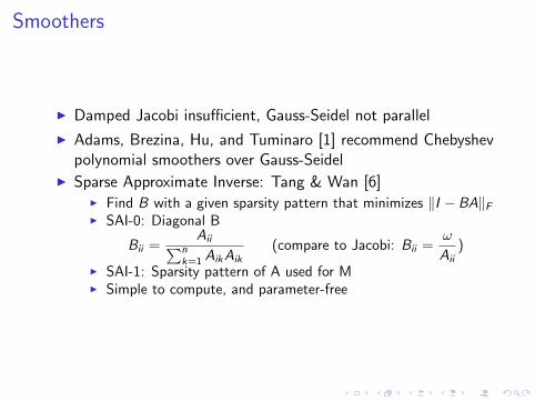
Smoothers

I Damped Jacobi insufficient, Gauss-Seidel not parallel

I Adams, Brezina, Hu, and Tuminaro [1] recommend Chebyshevpolynomial smoothers over Gauss-Seidel

I Sparse Approximate Inverse: Tang & Wan [6]I Find B with a given sparsity pattern that minimizes ‖I −BA‖F

I SAI-0: Diagonal B

Bii =Aii∑n

k=1 AikAik(compare to Jacobi: Bii =

ω

Aii)

I SAI-1: Sparsity pattern of A used for MI Simple to compute, and parameter-free

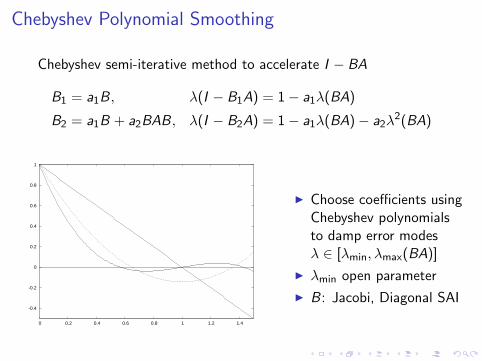
Chebyshev Polynomial Smoothing

Chebyshev semi-iterative method to accelerate I − BA

B1 = a1B, λ(I − B1A) = 1− a1λ(BA)

B2 = a1B + a2BAB, λ(I − B2A) = 1− a1λ(BA)− a2λ2(BA)

-0.4

-0.2

0

0.2

0.4

0.6

0.8

1

0 0.2 0.4 0.6 0.8 1 1.2 1.4

I Choose coefficients usingChebyshev polynomialsto damp error modesλ ∈ [λmin, λmax(BA)]

I λmin open parameter

I B: Jacobi, Diagonal SAI

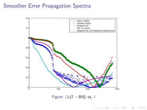
Smoother Error Propagation Spectra

0 500 1000 15000

0.2

0.4

0.6

0.8

1

1.2

1.4

Gauss−SeidelDamped JacobiDiagonal SAISAI, A’s stencilDiagonal SAI, 1st Chebyshev Improvement

Figure: |λi (I − BA)| vs. i

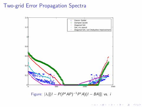
Two-grid Error Propagation Spectra

0 500 1000 15000

0.2

0.4

0.6

0.8

1

1.2

1.4

Gauss−SeidelDamped JacobiDiagonal SAISAI, A’s stencilDiagonal SAI, 1st Chebyshev Improvement

Figure: |λi [(I − P(P tAP)−1P tA)(I − BA)]| vs. i

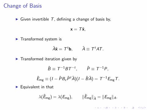
Change of Basis

I Given invertible T , defining a change of basis by,

x = T x,

I Transformed system is

Ax = T tb, A ≡ T tAT .

I Transformed iteration given by

B ≡ T−1BT−t , P ≡ T−1P,

Emg ≡ (I − PBc PtA)(I − BA) = T−1EmgT .

I Equivalent in that

λ(Emg) = λ(Emg), ‖Emg‖A = ‖Emg‖A.

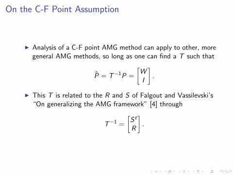
On the C-F Point Assumption

I Analysis of a C-F point AMG method can apply to other, moregeneral AMG methods, so long as one can find a T such that

P = T−1P =

[WI

].

I This T is related to the R and S of Falgout and Vassilevski’s“On generalizing the AMG framework” [4] through

T−1 =

[S t

R

].

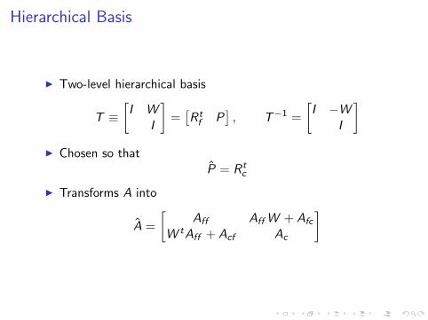
Hierarchical Basis

I Two-level hierarchical basis

T ≡[I W

I

]=

[Rt

f P], T−1 =

[I −W

I

]I Chosen so that

P = Rtc

I Transforms A into

A =

[Aff Aff W + Afc

W tAff + Acf Ac

]

Discrete Fundamental Solutions

I The transformed A,

A =

[Aff Aff W + Afc

W tAff + Acf Ac

],

is block-diagonal when the coarse basis functions are thediscrete fundamental solutions

W? = −A−1ff Afc .

I But W? is not sparse, hence not a viable choice. Introduce

F ≡ W −W?.

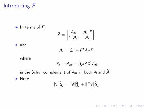
Introducing F

I In terms of F ,

A =

[Aff Aff F

F tAff Ac

],

I andAc = Sc + F tAff F ,

whereSc ≡ Acc − Acf A

−1ff Afc

is the Schur complement of Aff in both A and A.

I Note‖v‖2

Ac= ‖v‖2

Sc+ ‖Fv‖2

Aff.

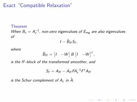
Exact “Compatible Relaxation”

TheoremWhen Bc = A−1

c , non-zero eigenvalues of Emg are also eigenvaluesof

I − Bff Sf ,

whereBff =

[I −W

]B

[I −W

]t,

is the ff -block of the transformed smoother, and

Sf = Aff − Aff FA−1c F tAff

is the Schur complement of Ac in A.

Two-grid Error Propagation Spectra

0 500 1000 15000

0.2

0.4

0.6

0.8

1

1.2

1.4

Gauss−SeidelDamped JacobiDiagonal SAISAI, A’s stencilDiagonal SAI, 1st Chebyshev Improvement

Figure: |λi [(I − P(P tAP)−1P tA)(I − BA)]| vs. i

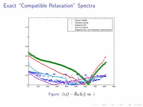
Exact “Compatible Relaxation” Spectra

0 100 200 300 400 500 600 700 800 9000

0.2

0.4

0.6

0.8

1

1.2

Gauss−SeidelDamped JacobiDiagonal SAISAI, A’s stencilDiagonal SAI, 1st Chebyshev Improvement

Figure: |λi (I − Bff Sf )| vs. i

Equivalent F-relaxation

Corollary

With an exact coarse grid correction, the spectrum of Emg is leftunchanged when the smoother B is replaced by the F-relaxation

BF-r = Rtf Bff Rf ,

where again,Bff =

[I −W

]B

[I −W

]t.

Coarse- and Smoother-space Energies

I Coarse-space operator Ac = Sc + F tAff F .

I Smoother-space operator Sf = Aff − Aff FA−1c F tAff .

I Coarse-space and smoother-space energies

‖v‖2Ac

= ‖v‖2Sc

+ ‖Fv‖2Aff

,

‖w‖2Sf

= ‖w‖2Aff

− ‖F tAff w‖2A−1

c,

are minimal and maximal for any vectors when F = O.

I Sf is close to Aff when F is “small”.

Exact “Compatible Relaxation” Spectra

0 100 200 300 400 500 600 700 800 9000

0.2

0.4

0.6

0.8

1

1.2

Gauss−SeidelDamped JacobiDiagonal SAISAI, A’s stencilDiagonal SAI, 1st Chebyshev Improvement

Figure: |λi (I − Bff Sf )| vs. i

Inexact Compatible Relaxation Spectra

0 100 200 300 400 500 600 700 800 9000

0.2

0.4

0.6

0.8

1

1.2

Gauss−SeidelDamped JacobiDiagonal SAISAI, A’s stencilDiagonal SAI, 1st Chebyshev Improvement

Figure: |λi (I − Bff Aff )| vs. i

Measuring F

I Define γ as an energy norm of F ,

γ ≡ supv 6=0

‖Fv‖Aff

‖v‖Ac

.

I This quantity appears in, e.g., Falgout, Vassilevski, andZikatanov [5] in the form

γ2 = supv 6=0

‖v‖2Ac− ‖v‖2

Sc

‖v‖2Ac

< 1

as the square of the cosine of the abstract angle between thehierarchical component subspaces.

How Closely Aff Approximates Sf

LemmaThe eigenvalues of A−1

ff Sf are real and bounded by

0 < 1− γ2 ≤ λ(A−1ff Sf ) ≤ 1.

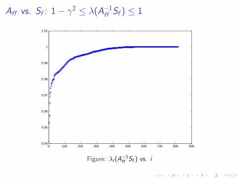
Aff vs. Sf : 1− γ2 ≤ λ(A−1ff Sf ) ≤ 1

0 100 200 300 400 500 600 700 800 9000.94

0.95

0.96

0.97

0.98

0.99

1

1.01

Figure: λi (A−1ff Sf ) vs. i

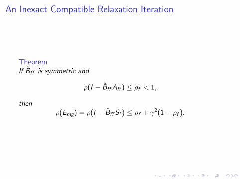
An Inexact Compatible Relaxation Iteration

TheoremIf Bff is symmetric and

ρ(I − Bff Aff ) ≤ ρf < 1,

thenρ(Emg) = ρ(I − Bff Sf ) ≤ ρf + γ2(1− ρf ).

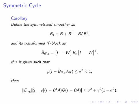
Symmetric Cycle

Corollary

Define the symmetrized smoother as

Bs ≡ B + Bt − BABt ,

and its transformed ff -block as

Bff ,s ≡[I −W

]Bs

[I −W

]t.

If σ is given such that

ρ(I − Bff ,sAff ) ≤ σ2 < 1,

then

‖Emg‖2A = ρ[(I − BtA)Q(I − BA)] ≤ σ2 + γ2(1− σ2).

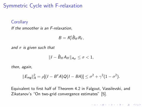
Symmetric Cycle with F-relaxation

Corollary

If the smoother is an F-relaxation,

B = Rtf Bff Rf ,

and σ is given such that

‖I − Bff Aff ‖Aff≤ σ < 1,

then, again,

‖Emg‖2A = ρ[(I − BtA)Q(I − BA)] ≤ σ2 + γ2(1− σ2).

Equivalent to first half of Theorem 4.2 in Falgout, Vassilevski, andZikatanov’s “On two-grid convergence estimates” [5].

AMG Iteration Design

I Central goal: make γ small

I Coarsening heursistic: make the columns of A−1ff decay quickly

I Prolongation: choose sparsity by cutting off −A−1ff Afc

according to some tolerance

I Smoother: simple F-relaxation of Aff

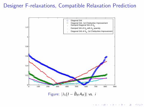
Designer F-relaxations, Compatible Relaxation Prediction

0 100 200 300 400 500 600 700 800 9000

0.2

0.4

0.6

0.8

1

1.2

Diagonal SAIDiagonal SAI, 1st Chebyshev ImprovementDamped Diagonal SAI of A

ffDamped SAI of A

ff with A

ff sparsity

Diagonal SAI of Aff, 1st Chebyshev Improvement

Figure: |λi (I − Bff Aff )| vs. i

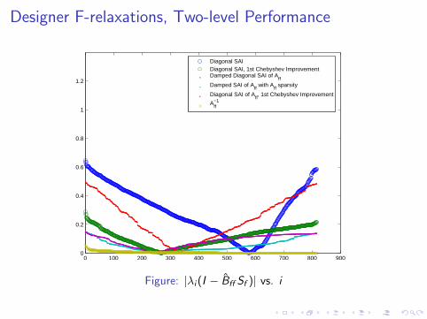
Designer F-relaxations, Two-level Performance

0 100 200 300 400 500 600 700 800 9000

0.2

0.4

0.6

0.8

1

1.2

Diagonal SAIDiagonal SAI, 1st Chebyshev ImprovementDamped Diagonal SAI of A

ff

Damped SAI of Aff with A

ff sparsity

Diagonal SAI of Aff, 1st Chebyshev Improvement

Aff−1

Figure: |λi (I − Bff Sf )| vs. i

M. Adams, M. Brezina, J. Hu, and R. Tuminaro.Parallel multigrid smoothing: polynomial versus Gauss-Seidel.Journal of Computational Physics, 188(2):593–610, 2003.

J. Brannick and L. Zikatanov.Domain Decomposition Methods in Science and EngineeringXVI, volume 55 of Lecture Notes in Computational Scienceand Engineering, chapter Algebraic multigrid methods basedon compatible relaxation and energy minimization, pages15–26.Springer Berlin Heidelberg, 2007.

O. Broker and M. J. Grote.Sparse approximate inverse smoothers for geometric andalgebraic multigrid.Applied Numerical Mathematics, 41(1):61–80, 2002.

R. D. Falgout and P. S. Vassilevski.On generalizing the algebraic multigrid framework.SIAM Journal on Numerical Analysis, 42(4):1669–1693, 2004.

R. D. Falgout, P. S. Vassilevski, and L. T. Zikatanov.On two-grid convergence estimates.Numerical Linear Algebra with Applications, 12(5–6):471–494,2005.

W.-P. Tang and W. L. Wan.Sparse approximate inverse smoother for multigrid.SIAM Journal on Matrix Analysis and Applications,21(4):1236–1252, 2000.

H. M. Tufo and P. F. Fischer.Fast parallel direct solvers for coarse grid problems.J. Par. & Dist. Comput., 61:151–177, 2001.

W. L. Wan, T. F. Chan, and B. Smith.An energy-minimizing interpolation for robust multigridmethods.SIAM Journal on Scientific Computing, 21(4):1632–1649,1999.

J. Xu and L. Zikatanov.

On an energy minimizing basis for algebraic multigridmethods.Computing and Visualization in Science, 7(3–4):121–127,2004.

Two-level Analysis

I Assume the coarse grid correction is exact,

Bc ≡ A−1c .

I The coarse grid correction

Q ≡ I − PA−1c PtA,

Q ≡ I − PA−1c PtA = I − Rt

cA−1c Rc A,

is a projection.

I The error propagation matrix spectrum is

λ(Emg) = λ[Q(I − BA)] = λ[(I − BA)Q].

Proof of First Theorem

I One may calculate

Q =

[I O

−A−1c F tAff O

],

AQ =

[Aff − Aff FA

−1c F tAff

O

]≡

[Sf

O

],

B ≡[Bff Bfc

Bcf Bcc

],

(I − BA)Q =

[I − Bff Sf O

−A−1c F tAff − Bcf Sf O

]I Sf is the Schur complement of Ac in A.

More on γ

I One may alternatively define

β ≡ supv 6=0

‖Fv‖Aff

‖v‖Sc

= ‖Rtf FRc‖A.

I The two quantities are related through

γ2 = supv 6=0

‖Fv‖2Aff

‖v‖2Sc

+ ‖Fv‖2Aff

= supv 6=0

‖Fv‖2Aff

/‖v‖2Sc

1 + ‖Fv‖2Aff

/‖v‖2Sc

=β2

1 + β2.

How Closely Aff Approximates Sf

LemmaThe eigenvalues of A−1

ff Sf are real and bounded by

0 < 1− γ2 ≤ λ(A−1ff Sf ) ≤ 1.

Proof.

A−1ff Sf = I − FA−1

c F tAff .

λ(A−1ff Sf ) = 1− λ(FA−1

c F tAff ) = 1− [{0} ∪ λ(A−1c F tAff F )].

0 ≤ infv 6=0

‖Fv‖2Aff

‖v‖2Ac

≤ λ(A−1c F tAff F ) ≤ sup

v 6=0

‖Fv‖2Aff

‖v‖2Ac

= γ2.