An active set solver for input-constrained robust recedinghorizon control
Johannes Buerger, Mark Cannon 1, Basil KouvaritakisDepartment of Engineering Science, University of Oxford, OX1 3PJ, UK
a r t i c l e i n f o
Article history:Received 7 August 2012Received in revised form28 May 2013Accepted 9 September 2013Available online 30 October 2013
Keywords:Robust controlControl of constrained systemsDynamic programmingMin–max optimal control
a b s t r a c t
An efficient optimization procedure is proposed for computing a receding horizon control law for linearsystems with linearly constrained control inputs and additive disturbances. The procedure uses an activeset approach to solve the dynamic programmingproblemassociatedwith themin–maxoptimization of anH∞ performance index. The active constraint set is determined at each sampling instant using first-ordernecessary conditions for optimality. The computational complexity of each iteration of the algorithmdepends linearly on the prediction horizon length. We discuss convergence, closed loop stability andbounds on the disturbance l2-gain in closed loop operation.
The aim of robust control is to provide guarantees of stabilityand of performance with respect to a suitable measure, despiteuncertainty in the model of the controlled system. Model Predic-tive Control (MPC) uses a receding horizon strategy to derive ro-bust control laws by repeatedly solving a constrained optimizationproblem online, and consequently the approach is effective for sys-tems with constraints and bounded disturbances.
Robust receding horizon control based on a worst-case opti-mizationwas proposed inWitsenhausen (1968). The approach em-ployed amin–max optimization, which was subsequently adoptedin Campo and Morari (1987) to derive an MPC law for linear sys-tems with uncertain impulse response coefficients. In this strat-egy, and in the related work (Allwright & Papavasiliou, 1992), anopen loop predicted future input sequence was used to minimizethe worst-case predicted performance. It was argued in Lee andYu (1997) that by optimizing instead over closed loop predictedinput sequences, control laws with improved performance andlarger regions of attraction could be obtained. However, unless a
The material in this paper was partially presented at the 50th IEEE Conferenceon Decision and Control (CDC), December 12–15, 2011, Orlando, Florida, USA. Thispaper was recommended for publication in revised form by Associate Editor MartinGuay under the direction of Editor Frank Allgöwer.
degree of optimality is sacrificed through the use of suboptimalcontroller parameterizations (such as, for example, those proposedin Goulart, Kerrigan, and Maciejowski (2006), Kothare, Balakrish-nan, andMorari (1996) and Löfberg (2003)), strategies that involvea receding horizon optimization over predicted feedback policiesgenerally require impractically large computational loads. For ex-ample Kerrigan and Maciejowski (2003) and Scokaert and Mayne(1998) apply a scenario-based approach to constrained linearsystems with bounded additive uncertainty, which leads to an op-timization problem in a number of variables which grows expo-nentially with the prediction horizon length.
Parametric solution methods aim to avoid the explosion incomputational complexity of robust dynamic programming withhorizon length by characterizing the solution of the recedinghorizon optimization problem offline, typically as a feedback lawthat is a piecewise affine function of themodel state. In (Bemporad,Borrelli, & Morari, 2003; Diehl & Björnberg, 2004) this methodwasapplied to linear systems with polytopic parametric uncertainty.However, whereas MPC typically solves an optimization problemfor a single initial condition at each instant, this approach requiresthe solution at all points in state space, and moreover necessitatesdetermining online which of a large number of polytopic regionscontains the current state.
This paper extends themethodology developed in Cannon, Liao,and Kouvaritakis (2008), Ferreau, Bock, and Diehl (2008) and Best(1996) to the case of linear systems with bounded additive uncer-tainty and input constraints in order to derive a robust dynamicprogramming solver. An online active set method is describedwhich avoids the need to compute the solution over the entire
156 J. Buerger et al. / Automatica 50 (2014) 155–161
state space, and which forms the basis of an efficient line-search-based point location technique. The control law is optimal for aconvex–concave min–max H∞ performance index, which ensuresclosed loop stability and a specified l2-disturbance gain bound. Thealgorithm’s computational complexity per iteration grows only lin-early with horizon length. We consider the case, which was pre-sented in Buerger, Cannon, and Kouvaritakis (2011), of systemssubject to constraints on control inputs alone; this paper providesfurther theoretical and numerical results and gives comparisonswithmax–min and open loop strategies, as well as numerical com-parison with the suboptimal min–max strategy of Goulart, Kerri-gan, and Alamo (2009).
2. Problem statement and notation
We consider linear discrete time systems with modelxt+1 = Axt + But + Dwt , t = 0, 1, . . . (1)with state xt ∈ Rnx , control input ut ∈ Rnu and disturbance inputwt ∈ Rnw at time t . Here ut and wt are subject to constraints:ut ∈ U,wt ∈ W , andU andW are assumed to be convex polytopicsets defined byU ,
u ∈ Rnu : Fu ≤ 1
W ,
w ∈ Rnw : Gw ≤ 1
for F ∈ RnF×nu , G ∈ RnG×nw , where 1 = [1 · · · 1]T denotes a vectorof conformal dimensions.
We define the feedback law u∗
N(x) as the solution to the follow-ing closed loop robust optimal control problem (Bemporad et al.,2003; Mayne, Raković, Vinter, & Kerrigan, 2006) over a finite hori-zon of N time-steps:u∗
m(x), w∗
m(x, u)
, argminu∈U
maxw∈W
Jm(x, u, w) (2a)
with Jm defined form = 1, 2, . . . ,N by
Jm(x, u, w) ,12(∥x∥2
Q + ∥u∥2R − γ 2
∥w∥2) + J∗m−1(x
+) (2b)
J∗m(x) , Jmx, u∗
m(x), w∗
m(x, u∗
m(x))
(2c)
where x+= Ax + Bu + Dw, with the terminal cost:
J∗0 (x) ,12∥x∥2
P . (2d)
Here R is a positive-definite matrix (denoted as R ≻ 0), Q is apositive-semidefinite matrix (Q ≽ 0), ∥x∥2
Q denotes xTQx, andthe scalar γ is chosen (as discussed in Section 3.1) to be suffi-ciently large that (2a) defines a strictly convex–concave min–maxproblem. We make the assumption that P is chosen so that∥x0∥2
P =
∞
t=0(∥xt∥2Q + ∥ut∥
2R − γ 2
∥wt∥2) with ut = uf
∞(xt) andwt = w
f∞(xt , ut), where uf
∞(·), wf∞(·) are the optimal solutions of
(2a)–(2c) in the limit as N → ∞ and in the absence of constraintsu ∈ U, w ∈ W . In order to guarantee the existence of this solu-tionwe assume that (A, B) is controllable and (Q 1/2, A) observable.Note that uf
∞(·), wf∞(·) can be computed by solving a semidefinite
programming problem (see e.g. Boyd, El Ghaoui, Feron, & Balakr-ishnan, 1994, for details).
The problem defined in (2a)–(2d) is formulated under the as-sumption that the disturbance wt is unknown when the controlinput ut is chosen at time t . Since the solutions u∗
m(·) andw∗m(·) de-
pend on x and on (x, u) respectively, (2a)–(2d) defines a closed loopoptimal control problem (see e.g. Lee & Yu, 1997). The sequentialnature of this min–max problem and the fact that the optimizationis performed over arbitrary feedback laws u∗
m(x), w∗m(x, u), m =
1, . . . ,N imply that, unlike open-loop formulations of robustMPC (e.g. Campo & Morari, 1987), (2a)–(2d) cannot be solved ex-actly by a single quadratic program.
For given x0, we denote the optimal state, input and distur-bance sequences as x(x0) = x0, . . . , xN, u(x0) = u0, . . . , uN−1,
w(x0) = w0, . . . , wN−1, where, for t = 0, . . . ,N − 1 we defineut = u∗
N−t(xt), wt = w∗
N−t(xt , ut) and xt+1 = Axt + But + Dwt .As discussed in Section 4, a receding horizon control law is
obtained by setting ut = u∗
N(xt) at each time t .
3. Active set solution via Riccati recursion
This section describes a method of solving (2a)–(2d) in orderto determine u∗
N(x) for a given plant state, x = xp. Thereforewe aim at determining a local solution to the closed-loop for-mulation of problem (2). For a given active set, we use a Riccatirecursion to solve the Karush–Kuhn–Tucker (KKT) conditions (No-cedal & Wright, 2006) providing first-order necessary optimalityconditions for problem (2). The optimal control and disturbanceinputs for the corresponding equality constrained problem are ob-tained as a sequence of affine state feedback functions. We givenecessary and sufficient conditions for optimality of these policieswith respect to problem (2). For the given active constraint set, ourapproach then determines state, control, disturbance and multi-plier sequences as functions of the initial state x0 using the systemmodel (1). As in Cannon et al. (2008), we use a line-search throughx0-space to update the active set, and the process is repeated un-til x0 = xp. This line-search is based on homotopy of solutions toproblem (2) and the solution can either be initialized using the un-constrained optimal control law with x0 = 0 or warm started us-ing the optimal solution for the plant state at the preceding timeinstant. Finally we discuss how the computation required by thisapproach depends on the problem size.
3.1. First order optimality conditions
Let λt and λt denote the Lagrange multipliers associated withthe constraints xt+1 = xt+1 +Dwt and xt+1 = Axt +But , and letµtand ηt denote the Lagrange multipliers for the constraints ut ∈ Uand wt ∈ W respectively.
Define Lagrangian functions for the stage-wise maximizationand minimization subproblems recursively as follows:
for the minimization subproblem, with terminal condition HN(xN)= J∗0 (xN) =
12∥xN∥
2P .
Lemma 1. The solution of problem (2) at time-step t satisfies
J∗N−t(xt) = min12∥xt∥2
Q +12∥ut∥
2R
+ Ht(xt+1, wt , ηt , λt , xt+1, . . . , xN)
(3)
where the minimization is over variables ut , xt+1, and wj, ηj, λj, xj+1
for j = t, . . . ,N − 1 and uj, µj, λj, xj+1 for j = t + 1, . . . ,N − 1and subject to the constraints: xt+1 = Axt + But , Fut ≤ 1, and∇wj Hj = 0, ∇xj+1 Hj = 0 for j = t, . . . ,N − 1, and ∇ujHj = 0,∇xj+1Hj = 0 for j = t + 1, . . . ,N − 1. Furthermore the objectiveof the maximization in (2) at time-step t, defined by J∗N−t(xt+1)
J. Buerger et al. / Automatica 50 (2014) 155–161 157
, −12γ
2∥w∗
N−t∥2+ J∗N−t−1(xt+1), satisfies
J∗N−t(xt+1) = max−
12γ 2
∥wt∥2
+Ht+1(xt+1, ut+1, µt+1, λk+1, xt+2, . . . , xN)
(4)
where themaximization is over variableswt , xt+1, and uj, µj, λj, xj+1,wj, ηj, λj, xj+1 for j = t+1, . . . ,N−1, and subject to the constraints:xt+1 = xt+1 + Dwt , Gwt ≤ 1, and µj ≥ 0, ηj ≥ 0, ∇wj Hj = 0,∇xj+1 Hj = 0, ∇ujHj = 0, ∇xj+1Hj = 0 for j = t + 1, . . . ,N − 1.
Theorem 2. The KKT conditions defining first order necessaryconditions for the optimal solution of problem (2) can be expressedas follows:
xt+1 = Axt + But + Dwt , t = 0, . . . ,N − 1 (5)
λt−1 = ATλt + Qxt , t = 1, . . . ,N − 1 (6)
and, for t = 0, . . . ,N − 1:
Rut = −BTλt − F Tµt (7a)
µt ≥ 0, µTt (1 − Fut) = 0, 1 − Fut ≥ 0 (7b)
γ 2wt = DTλt − GTηt (8a)
ηt ≥ 0, ηTt (1 − Gwt) = 0, 1 − Gwt ≥ 0 (8b)
with the terminal and initial conditions:
λN−1 = PxN (9)
x0 = xp. (10)
3.2. Riccati recursion
An active set approach solves the optimization problem (2) bysolving a sequence of problems involving only equality constraints.Let s = (su, sw) define a set of active constraints in (2), namely aset of constraints that are satisfied with equality at a solution of (2)for some initial state x0. Specifically, let su , su0,i, . . . , s
uN−1,i, i =
1, . . . , nF and sw , sw0,i, . . . , swN−1,i, i = 1, . . . , nG, where sut,i, s
wt,i
can take values of 0 or 1, and rewrite (7b) and (8b) as
eTi Fut = 1
eTi µt ≥ 0
if sut,i = 1, eTi Fut ≤ 1
eTi µt = 0
if sut,i = 0 (11)
eTi Gwt = 1eTi ηt ≥ 0
if swt,i = 1, eTi Gwt ≤ 1
eTi ηt = 0
if swt,i = 0 (12)
where ei denotes the ith column of an identity matrix of conformaldimensions. Also let Ft , Gt denote the matrices that consist of therows of F , G corresponding to the active sets indicated by sut,i = 1,i = 1, . . . , nF , and swt,i = 1, i = 1, . . . , nG, respectively, and denotethemultipliers of these active constraints asµa,t and ηa,t . Then theequality constraints in (7a), (11) and (8a), (12) are equivalent to
Rut = −BTλt − F Tt µa,t and Ftut = 1, (13)
γ 2wt = DTλt − GTt ηa,t and Gtwt = 1. (14)
Let Σ denote the set of all s such that (5), (6), (13), (14) are feasiblefor some x0. Then, for given s ∈ Σ , these constraints and (9), (10)define a two-point boundary value problem. To solve this equalityconstrained problemusing a Riccati recursion, we first assume that
λt may be expressed
λt = Ptxt+1 + qt . (15)
Then, using (5), (14) givesγ 2I − DTPtD GT
tGt 0
wtηa,t
=
DTPt(Axt + But) + DTqt
1
. (16)
Therefore, if (16) has the unique solution:wtηa,t
=
Mw
tMη
t
(Axt + But) +
mw
t
mηt
, (17)
then (15) gives λt = Pt(Axt + But) + qt with Pt , qt defined:
Pt = Pt + PtDMwt (18a)
qt = qt + PtDmwt (18b)
and hence (13) givesR + BT PtB F T
tFt 0
ut
µa,t
=
−BT PtAxt − BT qt
1
. (19)
Furthermore, assuming that (19) has a unique solution:ut
µa,t
=
LutLµt
xt +
lutlµt
, (20)
Eq. (6) yields λt−1 = Pt−1xt + qt−1, where
Pt−1 = Q + AT Pt(A + BLut ) (21a)
qt−1 = qt + AT PtBlut . (21b)
Finally, from (9) we have PN−1 = P and qN−1 = 0, and it followsby induction that (15) holds for t = N − 1, . . . , 0.
The necessary and sufficient conditions for optimality of theRiccati recursion in (17), (18) and (20), (21) are as follows.
Proposition 3. The optimal solution of (2a)–(2d) is given by
(where the columns of Ft,⊥ and Gt,⊥ form bases for the kernels of Ftand Gt respectively), and
GMw
t (Axt + But) + mwt
≤ 1, F(Lut xt + lut ) ≤ 1 (24a)
Mηt (Axt + But) + mη
t ≥ 0, Lµt xt + lµt ≥ 0. (24b)
Remark 4. Condition (23b) is necessarily satisfied since R ≻ 0 byassumption andQ ≽ 0 implies Pt , Pt ≻ 0 for all t . However (23a) isvery difficult to verify in practice, since thiswould require checkingall active sets s ∈ Σ . In this paper we therefore assume that γ
is sufficiently large to satisfy (23a) for all active sets likely to beencountered. We note that the terms Pt and qt define the optimalDP cost at stage N − t in the solution to problem (2) (omitting theconstant term for simplicity, since it has no effect on the solution).
158 J. Buerger et al. / Automatica 50 (2014) 155–161
3.3. Active set method
Using the feedback law (22) in conjunction with (5) to simulateforward over the N-step horizon, we obtain
xt = Φtx0 + φt for t = 1, . . . ,N (25)
where Φt ∈ Rn×n and φt ∈ Rn are given by
Φt+1 = (I + DMwt )(A + BLut )Φt (26a)
φt+1 = (I + DMwt )
(A + BLut )φt + Blut
+ Dmw
t (26b)
with initial conditions Φ0 = I and φ0 = 0. Therefore the in-put, disturbance and costate sequences u(x0), w(x0) and λ(x0) =
λ0, . . . , λN−1, as well as the corresponding multiplier sequencesµ(x0) = µ0, . . . , µN−1 and η(x0) = η0, . . . , ηN−1 can be de-termined as affine functions of x0 by substituting (25) into (17), (15)and (20). Hence, for a given active set s, we can define a region ofstate space X(s) ⊂ Rnx in which the KKT conditions hold:
X(s) ,x0 : x(x0) satisfies (24a,b)
. (27)
Lemma 5. The sets X(s) defined by (27) are convex polytopes, andthe collection X(s) : s ∈ Σ is a complex with the properties (seee.g. Grunbaum, 2000):
for any s1, s2 ∈ Σ (where ∂X(s) denotes the boundary of X). Fur-thermore the union ∪s∈Σ X(s) of all admissible active sets covers theset of feasible initial conditions for (2).
The algorithm we propose solves (2) based on a line-searchtechnique based on the homotopy of optimal solutions. Themethod is initialized by solving the equality constrained problemfor an optimal active set at some plant state x(0)
0 , and then updatesthis active set at successive iterations to find the optimal activeset at the current measured plant state xp. At each iteration j thealgorithm determines s(j+1) from s(j) by performing a line searchover x0 ∈ X(s(j)) in the direction of the current plant state xp. Con-straints are added to the active set by setting sut,i or s
wt,i to 1 when-
ever the corresponding inequality in (24a) (and hence (11), (12))becomes satisfied with equality. Constraints are dropped from theactive set by setting sut,i or s
wt,i to 0 if the corresponding multiplier
in (24b) (and (11), (12)) becomes equal to zero. This results in a se-quence of dual-feasible iterates x(i) that generate trajectories sat-isfying (24a,b) but not necessarily (10).
Algorithm 1. Initialize with x(0)0 and an active set s(0) such that
x(0)0 ∈ X(s(0)), and set j = 0. At iteration j = 0, 1, . . .:
(i) Compute Pt , qt for t = N − 1, . . . , 0, and Φt , φt for t =
0, . . . ,N − 1, and hence X(s(j)).(ii) Perform the line search:
α(j)= maxα∈(0,1]α : x(j)
0 + α(xp − x(j)0 ) ∈ X(s(j)).
(iii) If α(j) < 1, then set x(j+1)0 := x(j)
0 + α(j)(xp − x(j)0 ), j := j + 1,
and update s(j) on the basis of the new set of active constraints.Return to step (i).
(iv) Otherwise set s∗ := s(j), compute u∗
N(xp) and stop.
Theorem 6. Algorithm 1 converges after a finite number of iterationsto s∗ such that the trajectories for x, u and w generated by (1) and(22) with s = s∗ are optimal for (2).
Remark 7. If (2) is strictly convex–concave in the absence ofconstraints (i.e. if (23a,b) hold with Ft,⊥ = I and Gt,⊥ = I fort = 1, . . . ,N), then u∗
t (0) = 0 and w∗t (0, 0) = 0 for t = 1, . . . ,N ,
and hence a possible initialization of Algorithm 1 is x(0)0 = 0 and
s(0) = 0, . . . , 0.
Remark 8. In the context of MPC, the computation required byAlgorithm 1 may be reduced through warm-starting. For example,Algorithm 1 can be initialized at time t + 1 using the time-shiftedoptimal sequence computed at time t by setting x(0)
0 := Axt +
Bu∗
N(xt)+Dw∗
N(xt , u∗
N(xt)) and s(0) := s∗1(t), . . . , s∗
N(t), 0 at t+1,where s∗(t) is the optimal sequence of active sets at time t . Thechoice s∗N+1(t) = 0 corresponds to the assumption (discussed inSection 4) that the state of (5) enters a terminal set after N time-steps within which the unconstrained optimal control law andworst-case disturbances satisfy the constraints u ∈ U and w ∈ W .
3.4. Computation
In order to estimate how the computational complexity of Al-gorithm 1 depends on the problem size, we make the assumptionthat (16) and (19) are solved using the null space method com-monly employed by QP active set solvers (see e.g. Fletcher, 2000).This approach, applied to (16), involves computing the QR decom-position of Ft , which requires O(n2
w) floating point operations (as-suming that incremental rank-1 updates are employed), as well ascalculating the inverse of the matrix on the LHS of (23a), whichrequires O
(nw − nF )
3operations (assuming that Cholesky de-
composition is used), where nF ≤ nw is the number of rows of Ft .Applying the same approach to the solution of (19) requires O(n2
u)
operations for the QR decomposition of Gt plus O(nu − nG)
3op-
erations for the Cholesky decomposition of the LHS of (23b), wherenG ≤ nu is the number of rows of Gt . The other significant compu-tation in (17)–(21) is from the matrix multiplications in (18) and(21), which require O
(2n3
x + (3nu + 2nw)n2x + n2
unx)operations.
Combining these estimates, and noting that the computationrequired for the forward simulation is O(n2
xN) (since only the pro-jection, Φt(xp − x(i)
0 ), of Φt in (26a,b) is needed), and also that thecomputation involved in the line search in step (ii) is comparativelyinsignificant, we estimate the computation per iteration of Algo-rithm 1 to grow as
O
2n3x + n2
x(3nu + 2nw) + c1(n3w + n3
u) + c2(n2w + n2
u)N
.
Here c1, c2 are constants that depend on the implementation ofCholesky and QR decompositions, and we have used conservativeapproximations: nu − nG ≈ nu, nw − nF ≈ nw .
Thus the dependence of computation per iteration on thehorizon length N is linear. The required number of iterationsis problem-dependent and, in common with active solvers forquadratic programming, its upper bound is in general exponential,but empirical evidence (see the examples of Section 5) suggeststhat this also grows approximately linearly with N . Furthermorethe number of iterations can be minimized using warm-starting,as described in Remark 8. This is in stark contrast to existingschemes formin–max receding horizon control, which, for the caseof optimal approaches that are based on dynamic programming,have computational loads that necessarily depend exponentiallyon N (see e.g. Kerrigan & Maciejowski, 2003; Scokaert & Mayne,1998). Likewise, approaches such as Löfberg (2003), Goulart et al.(2006), Goulart et al. (2009) based on suboptimal controllerparameterizations require the solution of a convex optimization ina number of variables that grows quadratically with the horizonlength, which (as demonstrated in Section 5) leads to much highercomputational loads than Algorithm 1.
J. Buerger et al. / Automatica 50 (2014) 155–161 159
4. Closed loop stability and l2-gain bound
This section discusses the stability and disturbance attenuationproperties of the receding horizon controller defined by thesolution of problem (2). The problem description (2a)–(2d) doesnot include inequality state constraints, and hence it does notallow terminal state constraints to be included in the definition ofthe receding horizon policy. Nevertheless, the associated recedinghorizon control law u∗
N(·) ensures robust stability and induces aspecified disturbance l2-gain bound for a particular set of initialconditions. To show this we define a robust, controlled, positivelyinvariant set Xf under the infinite horizon unconstrained optimalsolutions, uf
∞(·), wf∞(·), of problem (2). The control law u∗
N(·)
ensures that the specified l2-gain bound holds for x0 ∈ XN , whereXN is a set of initial conditions fromwhichXf is reached inN stepsunder u = u∗
N(x). This section concludes with a discussion of theconnections betweenmin–max, max–min and open-loop problemformulations.
Definition 9. A set Xf ⊆ Rnx is robust positively invariant for(1) under ut = uf
∞(xt) and feasible for wt = wf∞(xt , u
f∞(xt)) if:
(i) uf∞(x) ∈ U for all x ∈ Xf ; (ii) Ax + Buf
∞(x) + Dw ∈ Xf for allx ∈ Xf , w ∈ W ; and (iii) w
f∞(x, uf
∞(x)) ∈ W for all x ∈ Xf .
Definition 10. For t = 1, . . . ,N , the set Xt is the preimage ofXt−1 for (1) under ut = u∗
N(xt) if X0= Xf and Xt
= x ∈ Rnx :
Ax + Bu∗
N(x) + Dw ∈ Xt−1, ∀w ∈ W.
Lemma 11. (i) Xf⊆ X1
⊆ · · · ⊆ XN ; (ii) XN is invariant anda region of attraction of Xf under u = u∗
N(x); (iii) for any k ≤ N,u∗
N(x) = u∗
k(x) ∀x ∈ Xk.
The main result of this section, concerning the stability of thedynamics xt+1 = Axt + But + Dwt , ut ∈ U, wt ∈ W , under thereceding horizon control law u = u∗
N(x), is stated next.
Proposition 12. If x0 ∈ XN , then, for any admissible disturbancesequence wt ∈ W, t = 0, 1 . . .: (i) the state of (1) with ut =
u∗
N(xt) satisfies xt ∈ Xf for all t ≥ N; (ii) the following l2-gain boundholds
∞t=0
(∥xt∥2Q + ∥ut∥
2R) ≤ γ 2
∞t=0
∥wt∥2+ 2J∗N(x0). (29)
4.1. Min–max, max–min and open loop problems
The formulation of problem (2) assumes that wt is unknownwhen ut is determined. If, on the other hand, ut is allowed to de-pend explicitly on wt , then it is straightforward to adapt Algo-rithm 1 to solve the max–min problem defined byw∗
m(x), u∗
m(x, w)
, argmaxw∈W
minu∈U
Jm(x, u, w), (30)
Jm(x, u, w) , 12 (∥x∥
2Q + ∥u∥2
R − γ 2∥w∥
2) + J∗m−1(x+), and J∗m(x) ,
Jmx, u∗
m(x, w∗m(x)), w∗
m(x), with terminal cost [b]J∗0 (x) , 1
2∥x∥2P .
It is easy to show that the receding horizon max–min control lawut = u∗
N(xt , wt) ensures the performance bound (29) with J∗N(x0)replaced by J∗N(x0). The additional information (i.e. knowledge ofwt ) needed to compute u∗
N(xt , wt) is expected to allow a smallerl2-gain bound; indeed this is demonstrated by the following result.
Theorem 13. For each active set s ∈ Σ , there exist scalars γ (s)and γ (s) such that for all x ∈ X(s) problem (2) is strictly convex–concave for γ ≥ γ (s) and problem (30) is strictly concave–convexfor γ ≥ γ (s), where γ (s) ≤ γ (s).
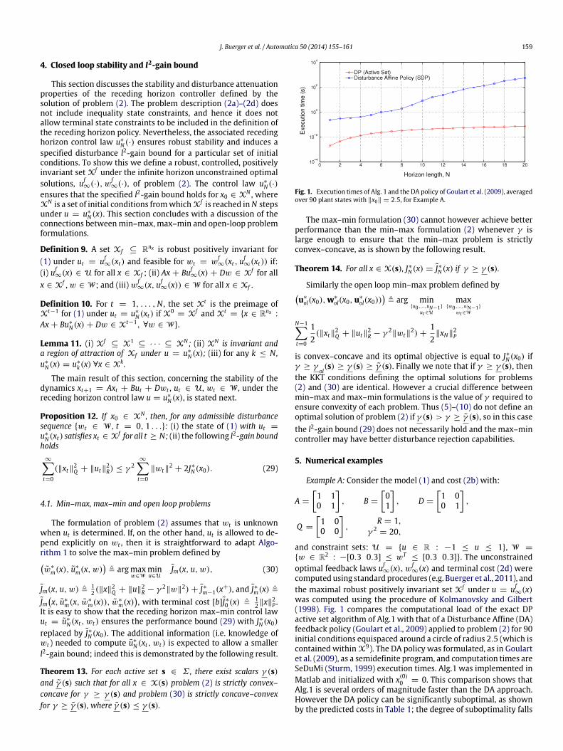
Fig. 1. Execution times of Alg. 1 and the DA policy of Goulart et al. (2009), averagedover 90 plant states with ∥x0∥ = 2.5, for Example A.
The max–min formulation (30) cannot however achieve betterperformance than the min–max formulation (2) whenever γ islarge enough to ensure that the min–max problem is strictlyconvex–concave, as is shown by the following result.
Theorem 14. For all x ∈ X(s), J∗N(x) = J∗N(x) if γ ≥ γ (s).
Similarly the open loop min–max problem defined byu∗
ol(x0),w∗
ol(x0,u∗
ol(x0))
, arg minu0,...,uN−1
ut∈U
maxw0,...,wN−1
wt∈W
N−1t=0
12(∥xt∥2
Q + ∥ut∥2R − γ 2
∥wt∥2) +
12∥xN∥
2P
is convex–concave and its optimal objective is equal to J∗N(x0) ifγ ≥ γ
ol(s) ≥ γ (s) ≥ γ (s). Finally we note that if γ ≥ γ (s), then
the KKT conditions defining the optimal solutions for problems(2) and (30) are identical. However a crucial difference betweenmin–max and max–min formulations is the value of γ required toensure convexity of each problem. Thus (5)–(10) do not define anoptimal solution of problem (2) if γ (s) > γ ≥ γ (s), so in this casethe l2-gain bound (29) does not necessarily hold and the max–mincontroller may have better disturbance rejection capabilities.
5. Numerical examples
Example A: Consider the model (1) and cost (2b) with:
A =
1 10 1
, B =
01
, D =
1 00 1
,
Q =
1 00 0
,
R = 1,γ 2
= 20,
and constraint sets: U = u ∈ R : −1 ≤ u ≤ 1, W =
w ∈ R2: −[0.3 0.3] ≤ wT
≤ [0.3 0.3]. The unconstrainedoptimal feedback laws uf
∞(x), wf∞(x) and terminal cost (2d) were
computedusing standard procedures (e.g. Buerger et al., 2011), andthe maximal robust positively invariant set Xf under u = uf
∞(x)was computed using the procedure of Kolmanovsky and Gilbert(1998). Fig. 1 compares the computational load of the exact DPactive set algorithm of Alg.1 with that of a Disturbance Affine (DA)feedback policy (Goulart et al., 2009) applied to problem (2) for 90initial conditions equispaced around a circle of radius 2.5 (which iscontained within X9). The DA policy was formulated, as in Goulartet al. (2009), as a semidefinite program, and computation times areSeDuMi (Sturm, 1999) execution times. Alg.1 was implemented inMatlab and initialized with x(0)
0 = 0. This comparison shows thatAlg.1 is several orders of magnitude faster than the DA approach.However the DA policy can be significantly suboptimal, as shownby the predicted costs in Table 1; the degree of suboptimality falls
160 J. Buerger et al. / Automatica 50 (2014) 155–161
Table 1Table 1. Comparison of initial predicted cost, closed loop cost for worst-case disturbances, and CPU time (s), for Example A with N = 12, for 25 initial conditions on theboundary of X12 .
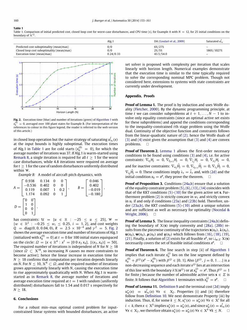
Fig. 2. Execution time (blue) and number of iterations (green) of Algorithm 1 withx(0)0 = 0, averaged over 100 plant states for Example B. (For interpretation of thereferences to colour in this figure legend, the reader is referred to the web versionof this article.)
in closed loop operation but the naive strategy of saturating uf∞(x)
at the input bounds is highly suboptimal. The execution timesof Alg.1 in Table 1 are for cold starts (x(0)
0 = 0), for which theaverage number of iterationswas 37. If Alg.1 is warm-started usingRemark 8, a single iteration is required for all t ≥ 1 for the worstcase disturbances, while 4.8 iterations were required on averagefor t ≥ 1 for the case of randomdisturbances uniformly distributedwithin W .
Example B: A model of aircraft pitch dynamics, with
w ∈ R2: −0.25 ≤ wi ≤ 0.25, i = 1, 2, and cost weights
Q = diag(0, 0, 0.04, 0), R = 2.5 × 10⁻⁴ and γ 2= 5. Fig. 2
shows the average execution time andnumber of iterations of Alg.1(initialized with x(0)
0 = 0) at t = 0 for 100 initial states equispacedon the circle: Ω = x ∈ R4
: xT = [0 0 x3 x4], ∥(x3, x4)∥ = 50.The required number of iterations is independent of N for N ≥ 18(since Ω ⊂ X18, so increasing N causes no more constraints tobecome active); hence the linear increase in execution time forN ≥ 18 confirms that computation per iteration depends linearlyon N . For N ≤ 10, XN
⊂ Ω , and the required number of iterationsgrows approximately linearly with N , causing the execution timeto rise approximately quadratically with N . When Alg.1 is warm-started as in Remark 8, the average number of iterations andaverage execution time required at t = 1 with random (uniformlydistributed) disturbances fall to 1.54 and 0.017 s respectively forN ≥ 18.
6. Conclusions
For a robust min–max optimal control problem for input-constrained linear systems with bounded disturbances, an active
set solver is proposed with complexity per iteration that scaleslinearly with horizon length. Numerical examples demonstratethat the execution time is similar to the time typically requiredto solve the corresponding nominal MPC problem. Though notconsidered here, extensions to systems with state constraints arecurrently under development.
Appendix. Proofs
Proof of Lemma 1. The proof is by induction and uses Wolfe du-ality (Fletcher, 2000). By the dynamic programming principle, attime t we can consider subproblems at t + 1, . . . ,N − 1 to in-volve only equality constraints (since an optimal active set existsfor these subproblems) and append the conditions correspondingto the inequality-constrained tth stage problem using the Wolfedual. Continuity of the objective function and constraints followsfrom the linear-quadratic nature of (2); hence the Wolfe duals of(3) and (4) exist given the assumption that (3) and (4) are convexproblems.
Proof of Theorem 2. Lemma 1 allows the first-order necessaryconditions to be found using conditions (3) and (4), i.e. for activeconstraints: ∇ujHj = 0, ∇xj+1Hj = 0, ∇λj
Hj = 0, ∇µjHj = 0,
and for inactive constraints: ∇wj Hj = 0, ∇xj+1 Hj = 0, ∇λj Hj = 0,∇ηj Hj = 0. These conditions imply λt = λt and, with (2d) and theinitial condition x0 = xp, they prove the theorem.
Proof of Proposition 3. Conditions (24a,b) ensure that a solutionof the equality constraint problem (5), (6), (13), (14) coincideswiththat of the KKT conditions (5)–(10) for the given active set s. Fur-thermore problem (2) is strictly concave in wt and strictly convexin ut if and only if conditions (23a) and (23b) hold. Therefore, un-der (23a,b), the KKT conditions (5)–(10) admit a unique solutionand are sufficient as well as necessary for optimality (Nocedal &Wright, 2006).
Proof of Lemma 5. The linear inequality constraints (24a,b) defin-ing the boundary of X(s) imply convexity and (28a). (28b) re-sults from the piecewise continuity of the trajectories x(x0), λ(x0),u(x0), w(x0), µ(x0) and η(x0) which follows from (16), (18), (19),(21). Finally, a solution of (2) exists for all feasible xp, so ∪s∈Σ X(s)necessarily covers the set of feasible initial conditions xp.
Proof of Theorem 6. The line search in step (ii) of Algorithm 1implies that each iterate x(j)
0 lies on the line segment defined byx(0)0 + β(j)(xp − x(0)
0 ) with β(j)∈ [0, 1]. Also β(j), j = 0, 1 . . . is a
non-decreasing sequence and each iterate x(j) lies at an intersectionof this linewith the boundary ∂X(s(j)) or at x(j)
0 = xp. Thus β(j)= 1
for finite j because the number of admissible active sets s ∈ Σ isfinite. It follows that Algorithm 1 terminates with x(j)
0 = xp.
Proof of Lemma 11. Definition 9 and the terminal cost (2d) implyu∗
N(x) = uf∞(x) ∀x ∈ Xf . Properties (i) and (ii) therefore
follow from Definition 10. We next demonstrate Property (iii) byinduction. Thus, if, for some k ≤ N , u∗
i (x) = u∗
N(x) ∀x ∈ Xi for alli < k, then x ∈ Xk implies u∗
k(x) = u∗
N(x), and since u∗
N(x) = uf∞(x)
∀x ∈ Xf , we therefore obtain u∗
k(x) = u∗
N(x) ∀x ∈ Xk∀k ≤ N .
J. Buerger et al. / Automatica 50 (2014) 155–161 161
Proof of Proposition 12. For x0 ∈ XN , Definitions 9, 10 andLemma 11 imply xt ∈ Xf for all t ≥ N and J∗N(xt) ≥ J∗N(xt+1) +12 (∥xt∥
2Q + ∥ut∥
2R − γ 2
∥wt∥2) for all t ≥ 0; the bound (29) follows
from this inequality (see e.g. Mayne et al., 2006).
Proof of Theorem 13. Problem (30) is strictly concave–convex fora given active set s if and only if:
F Tt,⊥(R + BT PtB)Ft,⊥ ≻ 0 (31a)
GTt,⊥(γ 2I − DT ˆP tD)Gt,⊥ ≻ 0 (31b)
where ˆP t = Pt − PtBLut , Pt−1 = Q + AT ˆP t(A + DMwt ) and
u∗
N−t(x, w) = Lut (Ax + Dw) + lwt , w∗
N−t(x) = Mwt x + mw
t fort = 0, . . . ,N − 1, with PN−1 = P . Since PN−1 = P and since u∗
m(x)and w∗
m(x) are suboptimal solutions for u∗m(x, w) and w∗
m(x, u)respectively, it follows by induction that Pt ≼ Pt for t = 0, . . . ,N−
1. Therefore λ(DT ˆP tD) ≤ λ(DTPtD) (λ(·) denotes minimumeigenvalue) and hence, for all t = 0, . . . ,N − 1, the lower boundon γ imposed by (23a) exceeds that imposed by (31b).
Proof of Theorem 14. If γ ≥ γ (s), then problem (2) is strictlyconvex–concave and the Wolfe dual permits reformulation as asingleminimization. The order inwhich u∗
m andw∗m are determined
can then be interchanged, and subsequent re-application of theWolfe dual, which is applicable since γ ≥ γ (s) by Theorem 13,yields problem (30).
References
Allwright, J. C., & Papavasiliou, G. C. (1992). On linear programming and robustmodel-predictive control using impulse-responses. Systems & Control Letters,18(2), 159–163.
Bemporad, A., Borrelli, F., & Morari, M. (2003). Min-max control of constraineduncertain discrete-time linear systems. IEEE Transactions on Automatic Control,48(9), 1600–1606.
Best, M. J. (1996). An algorithm for the solution of the parametric quadratic pro-gramming problem. In Applied mathematics and parallel computing (pp. 57–76).Heidelberg: Physica-Verlag.
Boyd, S., El Ghaoui, L., Feron, E., & Balakrishnan, V. (1994). Linear matrix inequalitiesin systemand control theory:Vol. 15. Studies in appliedmathematics. Philadelphia,PA: SIAM.
Buerger, J., Cannon, M., & Kouvaritakis, B. (2011). An active set solver for input-constrained robust receding horizon control. In 50th IEEE Conference on Decisionand Control, pp. 7931–7936.
Campo, P. J., & Morari, M. (1987). Robust model predictive control. Proc. AmericanControl Conference, pp. 1021–1026.
Cannon, M., Liao, W., & Kouvaritakis, B. (2008). Efficient MPC optimization usingPontryagin’s minimum principle. International Journal of Robust and NonlinearControl, 18(8), 831–844.
Diehl, M., & Björnberg, J. (2004). Robust dynamic programming for min-maxmodel predictive control of constrained uncertain systems. IEEE Transactionson Automatic Control, 49(12), 2253–2257.
Ferreau, H. J., Bock, H. G., & Diehl, M. (2008). An online active set strategy toovercome the limitations of explicit MPC. International Journal of Robust andNonlinear Control, 18, 816–830.
Fletcher, R. (2000). Practical methods of optimization. Wiley.
Goulart, P. J., Kerrigan, E. C., & Alamo, T. (2009). Control of constrained discrete-timesystems with bounded l2 gain. IEEE Transactions on Automatic Control, 54(5),1105–1111.
Goulart, P. J., Kerrigan, E. C., & Maciejowski, J. M. (2006). Optimization overstate feedback policies for robust control with constraints. Automatica, 42(4),523–533.
Grunbaum, B. (2000). Convex polytopes (2nd ed.). Springer.Kerrigan, E. C., &Maciejowski, J.M. (2003). Robustly stable feedbackmin-maxmodel
predictive control. In Proc. ACC, Denver, CO.Kolmanovsky, I., & Gilbert, E. (1998). Theory and computation of disturbance
invariant sets for discrete-time linear systems. Mathematical Problems inEngineering , 4, 317–367.
Kothare, M. V., Balakrishnan, V., & Morari, M. (1996). Robust constrainedmodel predictive control using linear matrix inequalities. Automatica, 32(10),1361–1379.
Lee, J. H., & Yu, Z. (1997). Worst-case formulations of model predictive control forsystems with bounded parameters. Automatica, 33.
Löfberg, J. (2003). Minimax approaches to robust model predictive control. Ph.D.thesis, Linköping University, Sweden.
Mayne, D. Q., Raković, S. V., Vinter, R. B., & Kerrigan, E. C. (2006). Characterizationof the solution to a constrained H∞ optimal control problem. Automatica, 42,371–382.
Nocedal, J., & Wright, S. (2006). Numerical optimization. Springer.Scokaert, P. O. M., & Mayne, D. Q. (1998). Min-max feedback model predictive
control for constrained linear systems. IEEE Trans. Automatic Control, 43(8),1136–1142.
Sturm, J. F. (1999). Using SeDuMi 1.02, a Matlab toolbox for optimization oversymmetric cones. Optimization Methods and Software, 11–12, 625–653.
Witsenhausen, H. (1968). A minimax control problem for sampled linear systems.IEEE Transactions on Automatic Control, 13, 5–21.
Johannes Buergerwas awarded an M.Eng. by the Univer-sity of Oxford in Engineering, Economics andManagementin 2008. In 2013 he obtained a D.Phil. in Engineering Sci-ence, also from the University of Oxford, for his work onefficient optimization techniques for Model PredictiveControl. He currently works as a control engineer for hy-brid powertrains at BMW, Munich.
Mark Cannon received the degrees of M.Eng. in Engineer-ing Science in 1993 and D.Phil. in Control Engineering in1998, both from the University of Oxford, and received theMS inMechanical Engineering in 1995 fromMassachusettsInstitute of Technology. He is anOfficial Fellow of St. John’sCollege and a University Lecturer in Engineering Science,Oxford University.
Basil Kouvaritakis was awarded a B.Sc. in Electrical Engi-neering from the University of Manchester Institute of Sci-ence and Technology, where he also received his Mastersand Doctorate. He is currently a Professor of Engineeringat the Department of Engineering Science and a TutorialFellow at St. Edmund Hall, Oxford University.