An Adaptive Flagellar Photoresponse Determines the Dynamics of Accurate Phototactic Steering in Chlamydomonas An Adaptive Flagellar Photoresponse 1 Determines the Dynamics of 2 Accurate Phototactic Steering in 3 Chlamydomonas 4 Kyriacos C Leptos 1†* , Maurizio Chioccioli 1†§ , Silvano Furlan 1¶ , Adriana I Pesci 1 , 5 Raymond E Goldstein 1* 6 *For correspondence: [email protected](KCL); [email protected](REG) † These authors contributed equally to this work Present address: § Department of Physics, University of Cambridge, JJ Thomson Avenue, Cambridge, CB3 0HE, UK; ¶ Sensing Electromagnetic Plus Corp., 2450 Embarcadero Way, Palo Alto, CA-94303, USA 1 Department of Applied Mathematics and Theoretical Physics, University of Cambridge, 7 Wilberforce Road, Cambridge, CB3 0WA, UK 8 9 Abstract Our understanding of phototaxis of biagellates stems almost exclusively from the 10 model alga Chlamydomonas reinhardtii, via studies of its agella, light-sensor and steering. However, 11 no comprehensive model linking all these aspects of its physiology and behavior has been 12 constructed and tested experimentally. Here, we develop such a mathematical model by coupling 13 an adaptive agellar photoresponse to rigid-body dynamics tailored to details of agellar beating, 14 and corroborate it with experimental data – at the agellar and tactic levels – to explain the 15 accurate phototactic steering of this alga. We experimentally validate the hypothesized adaptive 16 agellar photoresponse using high spatio-temporal resolution methodology on immobilized cells, 17 and corroborate the predicted reorientation dynamics of phototactic swimmers using 3D-tracking 18 of free-swimming cells. Finally, we reconrm, both theoretically and experimentally, that the 19 adaptive nature of the response has peak delity at a frequency of about 1.6 Hz, corresponding to 20 the rotation frequency of the cell body. 21 22 Introduction 23 Directional non-image-based phototaxis – the ability to change direction of motion in order to 24 reorient with a light stimulus – abounds in motile eukaryotic microorganisms, unicellular and multi- 25 cellular alike. From photosynthetic algae (Bendix, 1960) to early-stage larvae of marine zooplankton 26 (Thorson, 1964), phototaxis is such a crucial behavioral response for the survival of these organisms 27 that one is led to hypothesize that organisms must have evolved navigational strategies to reach 28 their goal in a very ecient manner. Photosynthetic algae need to harvest light energy to support 29 their metabolic activities, whereas animal larvae perform phototaxis so that their upward motion 30 can enhance their dispersal. 31 One of the most intriguing features of non-image-based phototaxis is the ability to navigate 32 towards (or away from) light without the presence of a central nervous system. One of the essential 33 sensory components for directional phototaxis (also known as vectorial phototaxis), is a specialized 34 sensor. This is possible in zooplanktonic larvae via a single rhabdomeric photoreceptor cell (Jékely 35 et al., 2008) or in the case of motile photosynthetic micro-organisms such as volvocalean algae, 36 a "light antenna" (Foster and Smyth, 1980), which was generally thought to co-localize with the 37 cellular structure called the eyespot, a carotenoid-rich orange stigma. Foster and Smyth (1980) 38 theorized that in order for vectorial phototaxis to work, the light antenna has to have directional 39 1 of 19 . CC-BY 4.0 International license peer-reviewed) is the author/funder. It is made available under a The copyright holder for this preprint (which was not . http://dx.doi.org/10.1101/254714 doi: bioRxiv preprint first posted online Jan. 27, 2018;
Transcript
An Adaptive Flagellar Photoresponse Determines the Dynamics of Accurate Phototactic Steering in Chlamydomonas
An Adaptive Flagellar Photoresponse1
Determines the Dynamics of2
Accurate Phototactic Steering in3
Chlamydomonas4
Kyriacos C Leptos1†*, Maurizio Chioccioli1†§, Silvano Furlan1¶, Adriana I Pesci1,5
Present address: §Department ofPhysics, University of Cambridge, JJThomson Avenue, Cambridge, CB30HE, UK; ¶Sensing ElectromagneticPlus Corp., 2450 Embarcadero Way,Palo Alto, CA-94303, USA
1Department of Applied Mathematics and Theoretical Physics, University of Cambridge,7
Wilberforce Road, Cambridge, CB3 0WA, UK8
9
Abstract Our understanding of phototaxis of bi�agellates stems almost exclusively from the10
model alga Chlamydomonas reinhardtii, via studies of its �agella, light-sensor and steering. However,11
no comprehensive model linking all these aspects of its physiology and behavior has been12
constructed and tested experimentally. Here, we develop such a mathematical model by coupling13
an adaptive �agellar photoresponse to rigid-body dynamics tailored to details of �agellar beating,14
and corroborate it with experimental data – at the �agellar and tactic levels – to explain the15
accurate phototactic steering of this alga. We experimentally validate the hypothesized adaptive16
�agellar photoresponse using high spatio-temporal resolution methodology on immobilized cells,17
and corroborate the predicted reorientation dynamics of phototactic swimmers using 3D-tracking18
of free-swimming cells. Finally, we recon�rm, both theoretically and experimentally, that the19
adaptive nature of the response has peak �delity at a frequency of about 1.6 Hz, corresponding to20
the rotation frequency of the cell body.21
22
Introduction23
Directional non-image-based phototaxis – the ability to change direction of motion in order to24
reorient with a light stimulus – abounds in motile eukaryotic microorganisms, unicellular and multi-25
cellular alike. From photosynthetic algae (Bendix, 1960) to early-stage larvae of marine zooplankton26
(Thorson, 1964), phototaxis is such a crucial behavioral response for the survival of these organisms27
that one is led to hypothesize that organisms must have evolved navigational strategies to reach28
their goal in a very e�cient manner. Photosynthetic algae need to harvest light energy to support29
their metabolic activities, whereas animal larvae perform phototaxis so that their upward motion30
can enhance their dispersal.31
One of the most intriguing features of non-image-based phototaxis is the ability to navigate32
towards (or away from) light without the presence of a central nervous system. One of the essential33
sensory components for directional phototaxis (also known as vectorial phototaxis), is a specialized34
sensor. This is possible in zooplanktonic larvae via a single rhabdomeric photoreceptor cell (Jékely35
et al., 2008) or in the case of motile photosynthetic micro-organisms such as volvocalean algae,36
a "light antenna" (Foster and Smyth, 1980), which was generally thought to co-localize with the37
cellular structure called the eyespot, a carotenoid-rich orange stigma. Foster and Smyth (1980)38
theorized that in order for vectorial phototaxis to work, the light antenna has to have directional39
1 of 19
.CC-BY 4.0 International licensepeer-reviewed) is the author/funder. It is made available under aThe copyright holder for this preprint (which was not. http://dx.doi.org/10.1101/254714doi: bioRxiv preprint first posted online Jan. 27, 2018;
An Adaptive Flagellar Photoresponse Determines the Dynamics of Accurate Phototactic Steering in Chlamydomonas
detection, i.e. detect light only on one side, and that the layers of carotenoid vesicles would act as40
an interference re�ector. This hypothesis was later veri�ed in algae by experiments of eyespot-less41
mutants that lacked the carotenoid vesicles, but could nevertheless do only negative phototaxis42
(Ueki et al., 2016). Their experiments concomitantly showed that the algal cell bodies can function43
as convex lenses with refractive indices greater than that of water. For the sake of completeness,44
it should be noted that in zooplankton the "shading" role of the carotenoid vesicles is �lled by a45
single shading pigment cell (Jékely et al., 2008).46
(a) (b)
c
c
t
t
t
c
Figure 1. Illustrations of the geometric model of a Chlamydomonas cell and of the two-phase model ofphototactic activity leading to steering. (a) The axes of the moving frame of the phototactic swimmer isshown, along with the position of the eyespot vector Ço, shown in red, and found at 45˝ away from the �agellarbeating plane spanned by Çe2 Çe3. The angular velocities !1 and !3 are also shown with p being the photoresponse,⇣ a hydrodynamic constant and fr the frequency of rotation of the cell body. (b) The two phases of photacticactivity responsinble for the persistence of phototactic reorientation. t represents the trans (in blue) and c thecis �agellum (in red).
Among photosynthetic algae the bi�agellate species Chlamydomonas reinhardtii has been the47
most studied organism: it exhibits, along with its breast-stroke mode of propagation (Rü�er and48
Nultsch, 1985) and left-handed helix rotation about its axis (Foster and Smyth, 1980), both positive49
(towards light) and negative (away from light) phototactic responses (Witman et al., 1993), as well as50
a photoshock/avoidance response. The eyespot in this alga is found on the equator of the cell and51
at 45˝ away from the plane of �agellar beating (Rü�er and Nultsch, 1985). It was in Chlamydomonas52
that the molecular players mediating phototaxis, the two eyespot-localized photoreceptors, chan-53
nelrhodopsins A and B, were discovered (Sineshchekov et al., 2002). The discovery that these54
proteins function as light-gated ion channels (Nagel et al., 2002), constituted the initial unraveling55
of Ariadne’s thread regarding the signal transduction pathway of the photoresponse. Starting56
instead in the center of this Minoan maze, Rü�er and Nultsch used high-speed cinematography to57
study the �agellar photoresponse (1990, 1991), including the photoshock response (1995). With58
their pioneering work on immobilized Chlamydomonas cells they showed, though using a negatively-59
phototactic strain, that the front amplitude of the cells was likely to be responsible for the steering of60
Chlamydomonas towards the light, and that phototaxis is a result of periodic irradiation and shading.61
This result led to the �rst model for phototaxis (Schaller et al., 1997) which divides the turning of62
the cell into two phases (Figure 1b): phase I, in which the rotating eyespot moves from shade to63
light, causing the �agellum farthest from the eyespot (the trans �agellum) to increase its amplitude64
relative to the �agellum next to the eyespot (the cis �agellum), and phase II, in which the eyespot65
moves from light to shade, leading to the two �agella acting in the opposite manner.66
Signi�cant contributions to the accuratemeasuring of �agellar photoresponse at a high temporal67
resolution weremade by Josef et al. (2005), who introduced a quadrature photodiode array, a device68
whose analog signal could be digitized at up to 4000 samples per second. Moreover, this automated69
2 of 19
.CC-BY 4.0 International licensepeer-reviewed) is the author/funder. It is made available under aThe copyright holder for this preprint (which was not. http://dx.doi.org/10.1101/254714doi: bioRxiv preprint first posted online Jan. 27, 2018;
An Adaptive Flagellar Photoresponse Determines the Dynamics of Accurate Phototactic Steering in Chlamydomonas
method could capture longer time series than previous methods. Despite the limitations of this70
technology to capture the �agellar photoresponse at high spatial resolution, the authors were able71
to extract important information regarding �agellar beat-frequency and stroke-velocity.72
In recent years, two types of models have sought to describe phototaxis: (i) numerical and73
theoretical models based on hydrodynamics and heuristic ciliary or �agellar response functions74
for ciliated larvae (Jékely et al., 2008) and bi�agellate algae (Bennett and Golestanian, 2015); (ii)75
theoretical adaptation-based models for the green alga Volvox (Drescher et al., 2010), the multicell-76
lular "relative" of Chlamydomonas. In this study, we have developed a comprehensive mathematical77
adaptation-based model, in the spirit of Drescher et al. (2010) and incorporating information from78
Schaller et al. (1997) and Rü�er and Nultsch (1991), coupled to the dynamics of the yaw, pitch, and79
roll of a rigid body in order to describe the three-dimensional phototaxis of Chlamydomonas cells.80
Moreover, we have developed new experimental techniques for capturing the �agellar photore-81
sponse of immobilized cells at high spatio-temporal resolution and to 3D-track the trajectories82
of free-swimming phototactic cells. Using these techniques we have measured the time scales83
involved in photoresponse, adaptation and reorientation that theory dictates are necessary for84
accurate phototaxis.85
Results86
Capturing �agellar photoresponse and phototactic steering87
The �agellar photoresponse of Chlamydomonas reinhardtii was captured at high spatio-temporal88
resolution using the experimental setup shown in Figure 2a. This setup builds on previous studies89
(Polin et al., 2009; Drescher et al., 2010; Leptos et al., 2013) with the addition of a much smaller90
optical �ber (�50 µm-core) to accommodate for the smaller size of a Chlamydomonas cell relative to91
a Volvox spheroid.92
The experimental setup (Figure 2b) used for phototactic steering featured the following modi�ca-93
tions relative to its predecessor (Drescher et al., 2009) – either engineered in-house or purchased –94
for ease and reproducibility: First, the sample chamber could be assembled by the user by clamping95
two acrylic �anges on a square glass tube in a watertight fashion to prevent leaks. The chamber96
design allowed a more accurate and easy calibration of the �eld of view and a simpler and better97
loading system of the sample via two barbed �ttings. Furthermore, the new design of the chamber98
minimized sample contaminations during experiments. Second, the two 5-Megapixel cameras99
coupled to objectives with higher total magni�cation (ù16) and larger working distance at the same100
magni�cation (48 mm vs. 38 mm at ù2) were used to enhance the image performance.101
Flagellar photoresponse is adaptive102
We start by applying a step-up light stimulus. The ability to record the �agellar dynamics of103
Chlamydomonas cells, during light stimulation and at high spatio-temporal resolution, revealed104
many interesting and important features of the �agellar photoresponse upon a stimulus of this form.105
Firstly, it corrobrated the fact that change in the waveform of the two �agella was in agreement with106
previous studies of high-speed cinematography (Rü�er and Nultsch, 1991), i.e. during a step-up107
response the front amplitude of the trans �agellum increases whereas the one of the cis �agellum108
decreases (Figure 3a-b). Secondly, it showed that the �agellar photoresponse is adaptive in nature109
(Figure 3c and Figure 3–Figure Supplement 2). For that reason we have employed a mathematical110
model, previously used to describe adaptive photoresponse in Volvox (Drescher et al., 2010), that111
relates the adaptive photoresponse p to a hidden slow-decaying variable h by means of the ordinary112
di�erential equations (ODEs):113
⌧r Üp = ⌘ s(t) * h * p (1a)
⌧a Üh = ⌘ s(t) * h (1b)
where s(t) is the photostimulus function and ⌘ is a factor with units reciprocal to s(t). The hidden114
variable h re�ects the internal biochemistry of the cell and is associated with a slower time scale ⌧a115
3 of 19
.CC-BY 4.0 International licensepeer-reviewed) is the author/funder. It is made available under aThe copyright holder for this preprint (which was not. http://dx.doi.org/10.1101/254714doi: bioRxiv preprint first posted online Jan. 27, 2018;
An Adaptive Flagellar Photoresponse Determines the Dynamics of Accurate Phototactic Steering in Chlamydomonas
(a)
(b)
filling aperture
1 mm ø capillary
x63 LWDwater-immersion lens
PDMS chamber
coverslipchamberaccess point
non-phototacticred light
optical fibercoupled to blue LED
CCD-camera #2
LWD-microscope #2
LWD-microscope #1
CCD-camera #1
red-light LED ring
red-light LED ring
outer tanksample chamber
optical fibercoupled to blue LED
Figure 2. Experimental setups. (a) Experimental setup for measuring the �agellar photoresponse on im-mobilized cells, inside a PDMS chamber, using a micropipette pulled to a �5-µm tip. In order to visualizethe cell’s beating �agella far from the coverslip, a ù63 LWD objective lens was used. The blue LED used forlight stimulation was coupled to a �50-µm optical �ber. (b) Experimental setup for 3D-tracking phototacticfree-swimming cells in a sample chamber immersed into an outer water tank for minimizing thermal convection.Imaging was performed using two aligned LWD microscopes, attached to two CCD cameras.
4 of 19
.CC-BY 4.0 International licensepeer-reviewed) is the author/funder. It is made available under aThe copyright holder for this preprint (which was not. http://dx.doi.org/10.1101/254714doi: bioRxiv preprint first posted online Jan. 27, 2018;
An Adaptive Flagellar Photoresponse Determines the Dynamics of Accurate Phototactic Steering in Chlamydomonas
1
0.5
0
-0.5
01
-1 0 1 2
PFD (μE.s -1.m
-2)
Time (s)
(c)1.5
2
(a) (b)
2
1
0
(d)
(s)
(s)0 0.05 0.1
Figure 3. Flagellar photoresponse of immobilized cells upon step-up light stimulation. The raw frontamplitudes Fcis and Ftrans (shaded areas in red for cis and blue for trans) as de�ned in the text for each �agellumare shown (a) before and (b) right after the beginning of the photostimulus. The 60˝ reference lines are alsoshown. Direction of light is from the left (blue arrow). Scale bar is 5 µm. (c) The mean (dark blue line) andstandard deviation (light-blue area) of photoresponse ( ÇFtrans * ÇFcis) during a step-up stimulus for one cell (ntech =4) �tted to Equation 2 (red line). (d) Inset showing the mean (red markers) and standard deviation (black errorbars) of �tted (⌧r, ⌧a) pairs for ncells = 4 upon step-up stimulation. The (⌧r, ⌧a) pair indicated with a black marker isderived from �tting the gain of the frequency response shown in Figure 4a. The hyperbolas for f opt
r = 1 Hz (red)and f opt
r = 2 Hz (green) are also shown.Figure 3–Figure supplement 1. Angle used to de�ne the beginning and the end of a beat. A chord isdrawn from the base of each �agellum to a point of �xed length on the �agellum. The angles ⇥cis and ⇥trans
between each of the chords (red for cis and blue for trans respectively) and the axis of symmetry of the cell(green), were used to de�ne the duration of the �agellar beats. Scale bar is 5�m.Figure 3–Figure supplement 2. Video showing �agellar photoresponse of immobilized cells upon step-up light stimulation. The optical �ber is illustrated as a grey square that turns blue when stimulus light isturned on. The curves �tted to the cis and trans �agella are shown in red and blue respectively.Figure 3–Figure supplement 3. Beat frequency �agellar photoresponse. The beat frequency response forthe same cell as shown in Figure 3c averaged over ntech = 4 movies. The instantaneous beat frequency wascalculated for each beat, ignoring beats that were out of synchrony. The mean and standard deviations of theinstantaneous frequencies of the cis and trans �agella are shown in red and blue respectively.
5 of 19
.CC-BY 4.0 International licensepeer-reviewed) is the author/funder. It is made available under aThe copyright holder for this preprint (which was not. http://dx.doi.org/10.1101/254714doi: bioRxiv preprint first posted online Jan. 27, 2018;
An Adaptive Flagellar Photoresponse Determines the Dynamics of Accurate Phototactic Steering in Chlamydomonas
(Equation 1b) than the fast response time scale ⌧r (Equation 1a). For a step-up stimulus s(t) = soH(t),116
where H(t) is the Heaviside function and so is the intensity (�ux density) of the light stimulus,117
these equations can be solved in closed form. Furthermore the data revealed a time-delay of118
photoresponse upon light stimulation, we therefore add a time delay td to this solution to obtain:119
pstep(t) =⌘ so
1 * ⌧r⌧a
0e*
(t*td )⌧a * e*
(t*td )⌧r
1H(t * td) (2)
We �t the photoresponse data to Equation 2 to the dimensionless observable p = ÇFtrans * ÇFcis, the120
di�erence of the normalized front amplitudes. The average front amplitude ÑF corresponding to121
each unstimulated cell – used for normalization – was found to be in the range of 35-45 µm2. The122
result of the �ttings allowed us to extract values for (⌧r, ⌧a) pairs, as shown in Figure 3d, with high123
accuracy. In order to quantify how these values can a�ect the e�ciency of the photoresponse of a124
free swimming cell rotating around its central axis, we derived a mathematical relationship relating125
⌧r and ⌧a to the frequency of an oscillating light stimulus fs (see next section):126
f opts = 1
2⇡˘⌧a⌧r
(3)
Mathematically this corresponds to the value of fs(= !s_2⇡), where the gain of rotational127
frequency responseR(!s) (described in Equation 5) is at its maximum. The relation in Equation 3128
describes a curve (a hyperbola) of optimal (⌧r, ⌧a) pairs for a given stimulus frequency fs for an129
immobilized cell, which can be considered equivalent to a rotational frequency fr of a free-swimming130
cell. As we see from Figure 3d, the mean values of �tted (⌧r, ⌧a) pairs along with their standard131
deviations, for the four cells analyzed, lie within the hyperbolas for f optr = 1 Hz (red) and f opt
r = 2 Hz132
(green).133
Another important feature of the step-up �agellar photoresponse is the time delay between134
stimulus and response. As shown in Figure 1a the eyespot (represented by a red square on the135
green sphere) is located at an angle ' = 45˝ away from the plane of �agellar beating (located in the136
Çe2 Çe3 plane). This means that upon light stimulus the �agella of the cell need to be pointing to the137
same direction as the eyespot for phototaxis to take place in an e�cient manner. For that reason138
we hypothesize that the �agellar response of the cell has been �ne-tuned by natural selection to139
have a delay such that the maximum photoresponse (pmax) will occur after the cell has rotated by an140
angle of ˘ 45˝ during its left-handed helix motion. According to Equation 2 the time tmax at which141
pmax occurs is:142
tmax = ln⌧a⌧r
0⌧a⌧r⌧a * ⌧r
1+ td (4)
Based on our data we compute tmax to be 94 ± 24 ms (n = 4), which corresponds to an fr = 1.1-1.8143
Hz, assuming a constant ' = 45˝, or to ' = 38 * 64˝, assuming a constant f optr = 1.5 Hz. The range of144
values for f optr are consistent with the locations of (⌧r, ⌧a) pairs in Figure 3d.145
Flagellar photoresponse is �ne-tuned with the frequency of rotation of cell body146
Cells were stimulated with oscillating light intensity for �ve di�erent frequencies. If the adaptive147
photoresponse model holds true, then there should be a maximum response at a resonant fre-148
quency corresponding to the frequency of rotation of the cell fr. This was shown in the past with149
di�erent techniques, both at the population level (Yoshimura and Kamiya, 2001) by measuring the150
bulk photoreceptor current, and at the single cell-level by Josef et al. (2006), for negative phototaxis151
and at low spatial resolution. Here we show that this is true at the single cell level, for positive152
phototaxis and at high spatial resolution, by directly measuring the �agellar photoresponse p as153
de�ned in the previous section. The results from individual experiments (Figure 4b-d) immediately154
revealed two major �ndings: (a) The �agellar photoresponse oscillates with the same frequency as155
the frequency of the amplitude of the light-stimulus. This means that the response is linear and can156
6 of 19
.CC-BY 4.0 International licensepeer-reviewed) is the author/funder. It is made available under aThe copyright holder for this preprint (which was not. http://dx.doi.org/10.1101/254714doi: bioRxiv preprint first posted online Jan. 27, 2018;
An Adaptive Flagellar Photoresponse Determines the Dynamics of Accurate Phototactic Steering in Chlamydomonas
be described by the solution poscill (Equation 12 inMaterials and Methods) of the governing equa-157
tions (Equation 1a and Equation 1b), for an oscillating light stimulus s(t) (green line in Figure 4b-d).158
(b) The amplitude of the observed p (blue line in Figure 4b-d) is higher at certain frequencies than159
others.160
PFD (μE.s -1.m
-2)
2 4 6 8 10Time (s)
1
1
1
(b)1
0
-11
0
-11
0
-1
(c)
(d)
0
0.08
0.12
0.2
0.04
0.16
0 2 4 6 8Stimulus frequency (Hz)
(a)
Gai
n of
Fre
quen
cy R
espo
nse
Figure 4. Frequency response of immobilized cells stimulated with oscillating-amplitude light. (a) Thecalculated gain of the frequency response (for positive phototaxis) for �ve stimulus frequencies (0.5, 1, 2, 4 and8 Hz) for ncells = 3 (blue) �tted to Equation 5 (red line). The photoresponse ( ÇFtrans - ÇFcis) shown (in blue) for threedi�erent stimulus frequencies (in green): 1 Hz (b), 2 Hz (c) and 4 Hz (d). The values of p for �agellar beats duringinstantaneous asynchronies were replaced by interpolated values based on neighbouring synchronous beats.The percentage of asynchronous beats during the time intervals shown were 7.6%, 10.6% and 35.3 % for (b), (c)and (d) respectively.
In order to investigate which of the �ve stimulus frequencies (fs) gives the most prominent161
�agellar photoreponse p we �rst derived a relationship (R) between fs (= !s_2⇡) and the magnitude162
of the Fourier transform of poscill. This is de�ned in Equation 13 of theMaterials and Methods. The163
result of the computation, which we refer to as the gain of the frequency response, is a function of !s:164
165
R(!s) =!s⌧at�
!2s⌧2a + 1
� �!2s⌧2r + 1
� (5)
At the experimental level, we calculated the observed gain of the frequency response (blue in166
Figure 4a), using a Discrete Fourier Transform on the observed p. The mean observed gain peaks167
at 2 Hz. The data were �tted to Equation 5 giving ⌧r ˘ ⌧a = 0.1 s, which peaks at ˘1.6 Hz (red in168
Figure 4a).169
Model of phototactic swimmers in three dimensions170
Naturally, the information gained from measuring the photoresponse of immobilized cells can be171
used, initially at least, to get an estimate of the angular velocity !1 of the cell (Figure 1a) during172
a phototactic turn. In particular, we would like to estimate the angle by which a free-swimming173
cell – starting at a direction of 90˝ to the light source – would turn during the �rst half turn of174
the rotation of the cell body about Çe3 (Figure 1a). For pedagogical reasons we provide a more175
detailed calculation of this estimate in Appendix 1 as motivation for the full mathematical model176
that follows.177
For this estimate we a consider a simpli�ed swimmer in Stokes �ow. The swimmer is composed178
of a spherical body of radius R, and two “�agella" in the shape of thin rods of length L. We compute179
the total torque (Equation 18 in Appendix 1) generated by each of the two �agella – during the180
7 of 19
.CC-BY 4.0 International licensepeer-reviewed) is the author/funder. It is made available under aThe copyright holder for this preprint (which was not. http://dx.doi.org/10.1101/254714doi: bioRxiv preprint first posted online Jan. 27, 2018;
An Adaptive Flagellar Photoresponse Determines the Dynamics of Accurate Phototactic Steering in Chlamydomonas
e�ective stroke of the beat – to be181
⌧1,2 =23⇣Úfba1,2L2 = 4
3⇣ÚfbA1,2L, (6)
where fb is the frequency of �agellar beating, ⇣Ú is the perpendicular viscous drag coe�cient, a1,2 is182
the amplitude of each �agellum, and A1,2 is the area swept by each �agellum (Appendix 1-Figure 1).183
The physical quantity that causes the cell to turn with angular velocity !1 about Çe1 is the di�erence184
in the torques (�⌧) generated by the two �agella, divided by the rotational drag coe�cient ⇣r.185
Assuming that during a photoresponse the amplitude of �agellum 1 (a1) is equal to a + b and of186
�agellum 2 (a2) is equal to a * b, where b is the amplitude di�erence from the unstimulated state a,187
then !1 becomes188
!1 = *�⌧⇣r
= *⌧1 * ⌧2⇣r
= * ⌧⇣r
2ba
(7)
We know that the �agellar amplitude oscillates if it experiences an oscillating stimulus (Figure 4c)189
so Equation 7 can be rewritten as190
!1(t) = * ⌧⇣r
2ab(t) = * ⌧
⇣r2abo sin (2⇡frt) (8)
where bo is the maximum �agellar amplitude di�erence and fr is the frequency of rotation of the191
body of the cell. If we integrate Equation 8 for the �rst half turn (HT) we will get the angle of192
phototactic turning (�HT) for that period of time during which bo is assumed to be constant. The193
result of the integration (Appendix 1) is194
�HT = 43⇡
⇣Ú⇣r
fbfrL2bo. (9)
If we substitute L = 10µm, bo = 1µm, a = 5µm, ⇣Ú = 2.6 ù 10*3 Pa.s (Appendix 1), ⇣r = 3pN.µm.s195
(Appendix 1), fb = 50Hz and fr = 2Hz into Equation 9 we get a �HT ˘ 0.9 rad ˘ 52˝. This means196
that even with this oversimpli�ed model of rod-shaped �agella, where the torque generated is197
overestimated, it is possible for the phototactic swimmer to reorient with the light source (i.e. turn198
52˝ about Çe1) within half turn of cell-body rotation (i.e. a turn of 180˝ about Çe3). Even though we do199
not formally de�ne the dimensionless variable p – used previously to describe the photoresponse –200
in terms of the torques (⌧1,2) generated by the two �agella, we nevertheless proceed to utilize this201
convenient variable to model the reorientation of the phototactic swimmers in three dimensions,202
by de�ning !1 to be proportional to p.203
The reorientation of phototactic swimmers – in three dimensions – can be described as a system204
of �ve nonlinear ODEs expressing, in addition to that of p and h (Equation 1a and Equation 1b),205
the time evolution of the three Euler angles of precession (�), nutation (✓) and rotation ( ) (Symon,206
1971). This is achieved by coupling the light stimulus s(t) with the amount of light received by the207
eyespot as the cell turns and rotates. Moreover, the coupling of the Euler angle dynamics to the208
photoresponse is achieved with the relation !1 = *(1_⇣ )p, where ⇣ is an e�ective viscosity, as shown209
in Figure 1a. We postponed the detailed derivation to Appendix 2.210
Using the assumption that the swimmer’s U-turn lies in a plane (Appendix 2), we reduce the211
problem to a system of three ODEs in which � describes the angle between the direction of the212
swimmer and the direction of the light stimulus. Moreover, we non-dimensionalize the equations213
by introducing the variables ↵ = ⌧a!r, � = ⌧r!r and � = so⌘, where !r, ⌧r, ⌧a, so, and ⌘ represent the214
physical quantities de�ned previously. By integrating for every ⇡ (i.e. half a turn of rotation) we215
compute a map for the integral of �, i.e. �n for every integer half-turn n. Then as shown in Appendix216
2:217
�n+1 =� cos�n
!r⇣
4A(*1)n 1 * q
n+1
1 * q(q + 1) + B(*1)n 1 * r
n+1
1 * r(r + 1) +H(cos n⇡)C ⇡
2
5+�n (10)
wherein
A = ↵�3
(1 + �2)2(↵ * �), B = ↵4
(1 + ↵2)2(� * ↵), C = ↵(↵ + �)
(1 + �2)(1 + ↵2),
8 of 19
.CC-BY 4.0 International licensepeer-reviewed) is the author/funder. It is made available under aThe copyright holder for this preprint (which was not. http://dx.doi.org/10.1101/254714doi: bioRxiv preprint first posted online Jan. 27, 2018;
An Adaptive Flagellar Photoresponse Determines the Dynamics of Accurate Phototactic Steering in Chlamydomonas
0 0.2 0.4 0.6 0.8 1.0 1.2 1.4 1.6 1.8 2.00.4
0.5
0.6
0.7
0.8
0.9
1.0
Time (s)
Ang
le (
rad/
)
(a)
(b)
0 0.05 0.1 0.150
0.1
0.2
0.3
0.4 (c)
0
50
100
0
100
200
050
100
S
T
(μm)(μm)
(μm
)(μ
m)
Figure 5. Phototactic swimmers tracked in three-dimensions. (a) The U-turn of a phototactic swimmershown as acquired in the 3D-tracking apparatus. Trajectory in black indicates the time before light stimulation,whereas trajectory in green indicates after. Blue arrows indicate the direction of the light. The cropped trajectoryused for �tting the reorientation dynamics (c) is bounded by the points from S to T. (b) The dynamics of thereorientation angle ⌦ (in blue) for the cropped trajectory satisfying ⇡_2 Õ ⌦ Õ ⇡ (shown in (a) from S to T) �ttedby a set of curves (mean and standard deviation in red) described by the iterated map in Equation 10, for aconvergent range of parameters. (c) Inset showing the means (black markers) of �tted ⌧r, ⌧a pairs (standarddeviations in red), plotted along the hyperbolas for f opt
r = 1 Hz (red line), 1.5 Hz (blue line) and 2 Hz (green line).Figure 5–Figure supplement 1. Video of a phototactic swimmer with angle of reorientation. The U-turnof a phototactic swimmer shown in a video with the angle of reorientation plotted below in real time. The colorsof the points on the trajectory of the cell before (black) and after (green) the light is on (t = 0) are re�ected in thecolor of the markers on the plot below.Figure 5–Figure supplement 2. Fitting parameter statistics. (a) Distribution of the �tted rotational frequencywith median = 1.78 Hz (n = 21). (b) Distribution of the optimal rotational frequency, as de�ned by Equation 3 andusing the �tted ⌧r and ⌧a pairs as shown in Figure 5c, withmedian = 1.61 Hz (n = 21). (c) Linear correlation between�tted fr (from (a)) and optimal fr (from (b)), shown as a �tted straight line (blue) of the form f opt
r = 0.62f f itr + 0.52.
(d) Distribution of the �tted reorientation constant � with median = 8.98 s*1 (n = 21).
9 of 19
.CC-BY 4.0 International licensepeer-reviewed) is the author/funder. It is made available under aThe copyright holder for this preprint (which was not. http://dx.doi.org/10.1101/254714doi: bioRxiv preprint first posted online Jan. 27, 2018;
Within the M = 6 pairs of recorded movies, we tracked 283 trajectories with durations greater222
than 10 s and which included the trigger frame. From those, 44 showed both positive phototaxis223
and included a full turn to ⌦ = ⇡ as shown in Figure 5a and Figure 5–Figure Supplement 1. These224
three-dimensional trajectories were cropped to any points for which ⇡_2 Õ ⌦ Õ ⇡ and which could225
then be �tted to Equation 10, using the relation ⌦ = � + ⇡, as shown in Figure 5b. Out of these, 21226
trajectories had good �ts (see Methods section for criterion) and the estimated four parameters227
(⌧r, ⌧a, fr = !r_2⇡ and � = �_⇣ ) of Equation 10 converged to a su�ciently narrow range of values.228
More speci�cally, pairs of the means of �tted ⌧r and ⌧a (Figure 5c) fall within the values of optimal229
response and adaptation time scales as described by Equation 3, mostly between the hyperbolas230
f optr = 1.5 Hz (blue line) and f opt
r = 2 Hz (green line). The distributions of the means of �tted values231
for the other two parameters fr and � are shown in Figure 5–Figure Supplement 2a and Figure 5–232
Figure Supplement 2d respectively. The median value for the �tted rotational frequency of the cell233
(fr) was found to be 1.61 Hz, in strong agreement with the maximum value of the �tted gain of234
frequency response in Figure 4a. Parameter � had a median value of 8.98 s*1 and it was found to235
be independent for the two di�erent light intensities used.236
Discussion237
This study has achieved three major goals: the development of modern methods to capture �agellar238
photoresponse at high spatio-temporal resolution, the measurement of important biochemical239
time scales for the understanding of phototaxis and lastly the integration of the above information240
through the development of a biochemistry-based model to accurately describe the phototactic241
behavior of Chlamydomonas in terms of the dynamics of reorientation to the light source in three242
dimensions.243
In addition, this study has addressed issues relating to past observations: With respect to the244
lag time td of the photoresponse, we have measured a value of 32 ± 9 ms (n = 4), very similar to the245
value 30-40 ms observed by Rü�er and Nultsch (1991). In addition, we argue that the maximum246
�agellar response would take place at tmax as shown in Equation 4, which adds a correction factor247
to td . This is important when assessing the e�ciency of the response with respect to the frequency248
of rotation of the cell body.249
Regarding the amount of light necessary for a �agellar photoresponse with a positive sign,250
we have converged, through trial and error, to ˘1 µE.s*1.m*2 at a wavelength of 470 nm. This251
value is much lower than in other photoresponse experiments (Josef et al., 2005) where ˘60252
µE.s*1.m*2 were used at a longer wavelength (543 nm). This is consistent with the sensitivity253
pro�le of channelrhodopsin-2 (Sineshchekov et al., 2002). More detailed studies on the wavelength254
sensitivity of the �agellar photoresponse should be carried out in order to reveal any possible255
wavelength dependencies on ⌧r, ⌧a or ⌘.256
Our experimental results – coming from di�erent methodologies – show either directly, from257
the gain of �agellar photoresponse under stimuli of di�erent oscillatory frequencies (Figure 4a)258
or indirectly, from the estimated values of ⌧r and ⌧a (Figure 3d, Figure 5c and Figure 5–Figure259
Supplement 2ab), that cells with rotational frequency in the range of ˘1-2 Hz would have the most260
optimal response.261
The optimality of the sensitivity of the photoresponse was �rst addressed by Yoshimura and262
Kamiya (2001), using a paralyzed-�agella mutant strain (pf14) and an electrophysiological approach263
on a bulk sample. In their experiments, a suspension of immotile cells was exposed to an oscillating264
light stimulus (500 nm) and the resulting photoreceptor current was measured in a cuvette attached265
10 of 19
.CC-BY 4.0 International licensepeer-reviewed) is the author/funder. It is made available under aThe copyright holder for this preprint (which was not. http://dx.doi.org/10.1101/254714doi: bioRxiv preprint first posted online Jan. 27, 2018;
An Adaptive Flagellar Photoresponse Determines the Dynamics of Accurate Phototactic Steering in Chlamydomonas
to two platinum electrodes. The experiment using relatively high light intensities observed a266
frequency response peak of 1.6 Hz when stimulated with ˘160 µE.s*1.m*2 and a frequency response267
peak of 3.1 Hz when stimulated with ˘40 µE.s*1.m*2. The former observation is in perfect agreement268
with our results in Figure 4a and in Figure 5–Figure Supplement 2ab even though we used light269
stimulus intensities of ˘1 µE.s*1.m*2 and ˘5-10 µE.s*1.m*2 respectively. We have not seen any270
evidence of cells having �agellar photoresponse dynamics that would corroborate the latter result271
of 3.1 Hz and this is a matter open to further investigation.272
Further studies on the optimality of the sensitivity of the photoresponse at the �agellar level273
were �rst carried out by Josef et al. (2006) on single cells of a negatively phototactic strain. The274
usage of the quadrature photodiode to measure stroke velocity was vital to the automation of the275
methodology, nevertheless it gave the magnitude of the velocity component parallel to the body276
axis only and at a particular position. In this study, it is the �rst time that the optimality of the277
photoresponse’s sensitivity is shown in a wild-type strain performing positive phototaxis, both at278
the �agellar level and at high spatio-temporal resolution, digitally capturing the full waveform of279
the response.280
Moreover, this study addressed the relationship of stimulus s to the photoresponse of Chlamy-281
domonas p using di�erential equations and a handful of parameters such as ⌧r and ⌧a corresponding282
to physical processes. Attempts to derive similar relationships between stimulus and photore-283
sponse (Josef et al., 2006) used linear system analysis. The result of such a signal-processing284
oriented method, usually includes a much larger number of estimated parameters necessary for285
the description of the system –without necessarily corresponding to any obvious physical quantities286
that can be easily measured.287
With respect to the range of values observed for ⌧a and ⌧r, they lie in the low-⌧r/high-⌧a region288
for step-up, mid-⌧r/mid-⌧a region for 3D-tracking and high-⌧r/low-⌧a region for rotational frequency289
response experiment. Possible explanations for these observations have to do with the dependence290
on the intensity of the stimulus (blue) light as well as the interference from the intensity of the291
background (red) light. It is worthy of commenting that the amount of background light in the292
immobilized high-resolution experiments is many orders of magnitude higher than the 3D-tracking293
experiments, and it could very well play a role to the above observations.294
The development of a comprehensive mathematical model linking physiology to behavior295
presents a platform begging for future perturbation-based experiments in order to dissect the296
mechanism of phototaxis and extend our biological knowledge of the system. The implementation297
of such a detailed model will require the discovery of many more currently unknown relations298
between variables, not just for the sake of completeness, but for exploring emerging mechanisms299
of physiological importance. One such an example is the physiological importance of the parameter300
of proportionality (⌘) between p and s (Equation 1a) as a measure of phototactic e�ciency and301
phototactic sign, and its dependence on the intensity of the light stimulus.302
Flagellar photoresponse – and by extension phototaxis – appears to be a very complex biological303
process encompassing many variables, as mentioned above. This is evident from the fact that304
experiments exhibited a high level of di�culty regarding multiple measurements on the same cells305
of elicited positive photoresponse. This has to do with our lack of understanding of long-term306
adaptation to darkness or phototactic light for that matter, topics that only recently have begun to307
be addressed (Arrieta et al., 2017).308
It is noteworthy to remark that a biochemistry-based model can explain the experimentally309
observed dynamics of phototactic reorientation in three-dimensions, in the absence of an explicit310
hydrodynamic model, and with !1 = *(1_⇣ )p being su�cient. Although it is evident that the torque311
generated by each �agellum is connected to the total swept area (A) as in Equation 6 or to the312
front amplitudes (F ) as in the experiments, and that successive di�erences in the corresponding313
�agellar torques are responsible for !1, a more detailed model where biochemistry is coupled to314
mechanical forces would be the subject of a further study. One example of improving the model315
could be the investigation of the dependence of �agellar torque to the �agellar beat frequency316
11 of 19
.CC-BY 4.0 International licensepeer-reviewed) is the author/funder. It is made available under aThe copyright holder for this preprint (which was not. http://dx.doi.org/10.1101/254714doi: bioRxiv preprint first posted online Jan. 27, 2018;
An Adaptive Flagellar Photoresponse Determines the Dynamics of Accurate Phototactic Steering in Chlamydomonas
(fb) as shown in Equation 6. We know from experiments that the frequency of �agellar beat does317
not change signi�cantly during the photoresponse experiments on immobilized cells (Figure 3–318
Figure Supplement 3 showing the cell with the most change to be ’10%), but not necessarily for319
free-swimming cells. Another example of including more detailed hydrodynamics, would be the320
formal de�nition of 1_⇣ , the proportionality constant between !1 and p. Interestingly from the �tted321
parameter � (= �_⇣ in Equation 10), we know that the product between � and 1_⇣ is of order 10322
(median value 8.98 s*1) and although we do not know the exact value of � (= so⌘), we can estimate323
it to be in the range of 4 < � < 7 based on the light intensities used. This allows us to place an324
estimate on 1_⇣ in the range of 1.3 < 1_⇣ < 2.3, and if we compare it to Equation 7 we can further325
relate it to the �uid mechanics via 1_⇣ = ⌧_⇣r ù F_A = 5.7 s*1, where F_A is empirically found to326
be ˘1/3.5. In this study, we declare this level of proximity, i.e. same order of magnitude, between327
observed and expected values of 1_⇣ , a success, and we leave a more accurate estimate of this328
variable to future, more detailed hydrodynamic models that similarly link physiology to behavior.329
Methods and Materials330
This is a detailed description of the materials and methods used for both types of experiments with331
immobilized and free-swimming cells and their corresponding analyses.332
Culture conditions333
Chlamydomonas wild-type cells (strain CC125 (Harris, 2009)) were grown axenically under pho-334
toautotrophic conditions in minimal media (Rochaix et al., 1988), at 23˝C under a 100 µE.s*1.m*2335
illumination in a 14:10 h light-dark cycle.336
Flagellar photoresponse of immobilized cells337
Cells were prepared as described previously (Leptos et al., 2013) – centrifuged, washed and gently-338
pipetted into a custom-made observation chamber made of polydimethylsiloxane (PDMS) as shown339
in Figure 2a. Chambers were mounted on a Nikon TE2000-U inverted microscope with a ù63 Plan-340
Apochromat water-immersion long-working-distance (LWD) objective lens (441470-9900; Carl Zeiss341
AG, Germany). Cells were immobilized via aspiration using a micropipette (B100-75-15; Sutter, USA)342
that was pulled to a �5-µm tip, and the �agellar beating plane was aligned with the focal plane of343
the objective lens via a rotation-stage. Video microscopy of immobilized cells was performed using344
a high-speed camera (Phantom v341; Vision Research, USA) by acquiring 15 s-movies at 2000 fps.345
Cells were stimulated at exactly frame 2896 (˘1.45 s into the recording) using a �50 µm-core optical346
�ber (FG050LGA; Thorlabs, USA) that was coupled to a 470 nm Light Emitting Diode (LED) (M470L3;347
Thorlabs, USA) and was controlled via an LED driver (LEDD1B; Thorlabs, USA). The LED driver and348
the high-speed camera were triggered through a data-acquisition card (NI PCIe-6343; National349
Instruments, USA) using in-house programs written in LabVIEW 2013 (National Instruments, USA),350
for both step- and frequency-response experiments. Calibration of the optical �ber was performed351
as follows: A photodiode (DET110; Thorlabs, USA) was used to measure the total radiant powerW352
emerging from the end of the optical �ber for a range of voltage output values (0-5 V) of the LED353
driver. Subsequently, the two quantities were plotted and �tted to a power-law model which was354
close to linear.355
A stimulus of ˘1 µE.s*1.m*2 (at 470 nm) was empirically found to give the best results in terms356
of reproducibility, sign, i.e. positive phototaxis, and quality of response, since we conjecture that the357
cells could recover in time for the next round of stimulation. For the step response experiments,358
biological replicates were ncells = 4 with corresponding technical replicates ntech = {4, 3, 2, 2}. For the359
frequency response experiments, biological replicates were ncells = 3 with each cell stimulated to360
the following amplitude-varying frequencies: 0.5 Hz, 1 Hz, 2 Hz, 4 Hz and 8 Hz. Only the cells that361
showed a positive sign of response for all 5 frequencies are presented here. This was hence the362
most challenging aspect of the experimental process.363
12 of 19
.CC-BY 4.0 International licensepeer-reviewed) is the author/funder. It is made available under aThe copyright holder for this preprint (which was not. http://dx.doi.org/10.1101/254714doi: bioRxiv preprint first posted online Jan. 27, 2018;
with two In�niProbeTM TS-160 (In�nity, USA) with Micro HM objectives at a total magni�cation of ù16.391
The source of phototactic stimulus was a 470 nm blue-light LED (M470F1; Thorlabs, USA) coupled to392
a solarization-resistant optical �ber (M22L01; Thorlabs, USA) attached to an in-house assembled393
�ber collimator that included a �12.7 mm plano-convex lens (LA1074-A; Thorlabs, USA). Calibration394
of the collimated optical �ber was performed similarly to the experiments with immobilized cells. In395
addition, the thickness of the walls of the outer water tank, the walls of the inner sample chamber396
and the water in between, were taken into account for the calibration.397
The two CCD cameras and the blue-light LED used for the stimulus light were controlled using398
LabVIEW 2013 (National Instruments, USA) including the image acquisition driver NI-IMAQ (National399
Instruments, USA). The cameras were triggered and synchronized at a frame rate of 10 Hz via a data-400
acquisition device (NI USB 6212-BNC; National Instruments, USA). For every tracking experiment401
(M = 6), two 300-frame movies were acquired (side and top) with the phototactic light triggered at402
frame 50 (5 s into the recording). The intensity of the blue-light stimulus was chosen to be 5 or 10403
µE.s*1.m*2.404
13 of 19
.CC-BY 4.0 International licensepeer-reviewed) is the author/funder. It is made available under aThe copyright holder for this preprint (which was not. http://dx.doi.org/10.1101/254714doi: bioRxiv preprint first posted online Jan. 27, 2018;
.CC-BY 4.0 International licensepeer-reviewed) is the author/funder. It is made available under aThe copyright holder for this preprint (which was not. http://dx.doi.org/10.1101/254714doi: bioRxiv preprint first posted online Jan. 27, 2018;
Yoshimura K, Kamiya R. The sensitivity of Chlamydomonas photoreceptor is optimized for the frequency of cell483
body rotation. Plant and Cell Physiology. 2001 jun; 42(6):665–672. doi: 10.1093/pcp/pce084.484
15 of 19
.CC-BY 4.0 International licensepeer-reviewed) is the author/funder. It is made available under aThe copyright holder for this preprint (which was not. http://dx.doi.org/10.1101/254714doi: bioRxiv preprint first posted online Jan. 27, 2018;
An Adaptive Flagellar Photoresponse Determines the Dynamics of Accurate Phototactic Steering in Chlamydomonas
Appendix 1485
Calculations used in estimating the angle of phototactic turning486
Derivation of time-averaged total torque generated by rod-shaped �agella487
488
489
Appendix 1 Figure 1. Model of the e�ectivestroke of a simpli�ed swimmer. The total an-gle spanned by the rod-shaped �agella duringan e�ective stroke is equal to �b = a_L and thecorresponding swept area (shaded) is A = aL
2 .
490
491
492
493
494495
496
In order to derive the amount of phototacticturning per half turn of cell rotation, we con-sider a swimmer in Stokes �ow with a spher-ical body of radius R, bearing two rod-shaped�agella of length L attached at the anterior ofthe cell body, as shown in Appendix 1-Figure1. The swimmer is immersed in a �uid with vis-cosity ⌘. Furthermore, the swimmer �aps itsrod-shaped �agella with a maximum velocityat the tip equal to
utip =atb
(14)
where a is the amplitude of the beat and tbis the duration of the e�ective stroke of thebeat. We can thus assign each �agellum aforce-density function depending on the posi-tion � along the �agellum:
f (�) = ⇣Úu(�) = ⇣Ú�Lutip = ⇣Ú
�Latb, (15)
497
498
499
500
501
502
503
504
505
506
507
508
509
510
511
512
513
514
515
516
517
(a) (b)
518
519
Appendix 1 Figure 2. Geometric proof of the torque generated by a point on the rod-shaped�agellum. The proof is broken down in two parts: (a) for angles of � above the tangent AM to the cellbody (front amplitude) and (b) for angles of � below the same line (back amplitude).
520
521
522523
The corresponding torque density, according to the geometric proof shown in Appendix1-Figure 2a, for the front amplitude is
⌧F (�) = f (�) cos ↵ l =⇣ÚaLtb
�(� + R sin�)
where OA = R, AC = AM = L, AB = �, OB = l and l cos ↵ = BA® = AB + AA® = � + R sin�.
524
525
526
527
528
529
16 of 19
.CC-BY 4.0 International licensepeer-reviewed) is the author/funder. It is made available under aThe copyright holder for this preprint (which was not. http://dx.doi.org/10.1101/254714doi: bioRxiv preprint first posted online Jan. 27, 2018;
We would like to estimate the angle by which the cell turns – about its Çe1 axis – for theduration of half a turn about its Çe3 axis, while its angular velocity !1 oscillates as shown inEquation 8. It is reasonable to assume that the di�erence in �agellar amplitude betweenthe two �agella (2b), on which !1 depends, oscillates with constant amplitude (2bo) during theperiod of half a turn. Then we can compute the angle turned about Çe1 during the time thecell turns by an angle ⇡ about Çe3, by integrating Equation 8 over time from 0 to 1
2fr:
�HT = 1
2fr
0!1(t)dt = * ⌧
⇣r
2boa
12fr
0sin (2⇡frt)dt = * ⌧
⇣r
2boa
4*cos (2⇡frt)
2⇡fr
5 12fr
0
= ⌧⇣r
2boa
4* 12⇡fr
(*1 * (1))5= ⌧⇣r
2boa
22⇡fr
= ⌧⇣r
2boa
1⇡fr
If we substitute for ⌧ then we have
�HT = 23⇣ÚfbaL2 1
⇣r
2boa
1⇡fr
= 43⇡
⇣Ú⇣r
fbfrL2bo (19)
567
568
569
570
571
572
573
574
575
576
577
578
579
580
581
582
17 of 19
.CC-BY 4.0 International licensepeer-reviewed) is the author/funder. It is made available under aThe copyright holder for this preprint (which was not. http://dx.doi.org/10.1101/254714doi: bioRxiv preprint first posted online Jan. 27, 2018;
An Adaptive Flagellar Photoresponse Determines the Dynamics of Accurate Phototactic Steering in Chlamydomonas
Appendix 2583
Derivation of mathematical model584
The mathematical model is derived from a system of �ve nonlinear ordinary di�erentialequations (ODEs) following a series of simpli�cations and approximations. The �rst simpli�-cation is regarding the photoresponse time delay td , as mentioned in the main text. We knowfrom solving the equations numerically that including the time delay into the mathematicalmodel is equivalent to omitting it, but with the eyespot vector Ço lying on the ( Çe2 Çe3) plane,i.e. Ço = Çe2 (Figure 1a).
585
586
587
588
589
590
More speci�cally, the dynamics of the photoresponse (described by Equation 1a andEquation 1b) are coupled to the Euler angle dynamics via the light intensity relation *Çl � Ço =*so (sin cos� + cos ✓ sin� cos ), where Çl = * Çe
x
(Figure 5a), and the equations describingthe Euler angle dynamics (Symon, 1971) are coupled to the photoresponse via the relation!1 = *(1_⇣ )p, where ⇣ is a time scale constant equal to an e�ective viscosity. This gives thefollowing system of ODEs:
Ü� = *(1_⇣ )p sin sin ✓
, (20a)
Ü✓ = *(1_⇣ )p cos , (20b)
Ü = *2⇡fr + (1_⇣ )p sin sin ✓
cos ✓, (20c)
Üp = (1_⌧r)�*so⌘ (sin cos� + cos ✓ sin� cos )H(sin cos� + cos ✓ sin� cos ) * h * p
�, (20d)
Üh = (1_⌧a)�*so⌘ (sin cos� + cos ✓ sin� cos )H(sin cos� + cos ✓ sin� cos ) * h
�. (20e)
591
592
593
594
595
596
597
598
599
Using the test case where the initial direction of the cell is * Çe
y
, i.e. Euler angle initialconditions ✓ = ⇡_2 and � = 0, we conclude from the solution of the reorientation dynamicsthat the cell maintains a trajectory on the ( Çe
x
Çe
y
) plane with ✓ being almost constant. With✓ being constant and = *2⇡frt (Figure 1) we can reduce the number of equations in thesystem from �ve to three:
Ü� = (1_⇣ )p sin(2⇡frt), (21a)
Üp = (1_⌧r)�so⌘
�sin(2⇡frt) cos�
�H
�sin(2⇡frt) cos�
�* h * p
�, (21b)
Üh = (1_⌧a)�so⌘
�sin(2⇡frt) cos�
�H
�sin(2⇡frt) cos�
�* h
�. (21c)
600
601
602
603
604
605
606
607
The nondimensionalization of time Ét = !rt, where !r = 2⇡fr transforms the equations to
�Ét = (1_!r⇣ )p sin Ét, (22a)
pÉt = (1_⌧r!r)�so⌘
�sin Ét cos�
�H
�sin Ét cos�
�* h * p
�, (22b)
hÉt = (1_⌧a!r)�so⌘
�sin Ét cos�
�H
�sin Ét cos�
�* h
�. (22c)
608
609
610
611
To be able to decouple � from h and p, we assume that it does not change signi�cantlyduring a full (or half) cell rotation, and thus we solve the equations for h and p for a givenvalue of �.
612
613
614
If we let ↵ = ⌧a!r, � = ⌧r!r, � = so⌘ and dropping tildes, we can rewrite the equations asfollows:
615
616
↵ht + h = � sin t cos�H (sin t) , (23a)
�pt + p = � sin t cos�H (sin t) * h. (23b)
617
618
619
620
18 of 19
.CC-BY 4.0 International licensepeer-reviewed) is the author/funder. It is made available under aThe copyright holder for this preprint (which was not. http://dx.doi.org/10.1101/254714doi: bioRxiv preprint first posted online Jan. 27, 2018;
An Adaptive Flagellar Photoresponse Determines the Dynamics of Accurate Phototactic Steering in Chlamydomonas
Equation 23a can be rewritten as,
↵ht + h =
T� sin t cos� for n⇡ Õ t Õ (n + 1)⇡, where n Œ 0 is even0 for n⇡ Õ t Õ (n + 1)⇡, where n Œ 1 is odd
621
622
623
624
and it can be solved in a piecewise fashion to yield,
hn =hnlnj
K⇠
1*rn+1
1*re*
t*n⇡↵ + 1
↵sin t * cos t
⇡for n⇡ Õ t Õ (n + 1)⇡, where n Œ 0 is even
K⇠
1*rn+1
1*re*
t*n⇡↵
⇡for n⇡ Õ t Õ (n + 1)⇡, where n Œ 0 is odd
625
626
627
628
where
K = ↵� cos�1 + ↵2
andr = e*
⇡↵ .
629
630
631
632
633
634
635
636
Likewise, Equation 23b can be rewritten more analytically as637
�pt + p =
T� sin t cos� * hn for n⇡ Õ t Õ (n + 1)⇡, where n Œ 0 is even*hn for n⇡ Õ t Õ (n + 1)⇡, where n Œ 1 is odd
638
639
640
641
and it can be solved in a piecewise fashion as to yield,
pn =hnlnj
⇤11*qn+1
1*qe*
t*n⇡� + ⇤2 sin t + ⇤3 cos t + ⇤4
1*rn+1
1*re*
t*n⇡↵ for n⇡ Õ t Õ (n + 1)⇡, where n Œ 0 is even
⇤11*qn+1
1*qe*
t*n⇡� + ⇤4
1*rn+1
1*re*
t*n⇡↵ for n⇡ Õ t Õ (n + 1)⇡, where n Œ 0 is odd
642
643
644
645
where
⇤1 =↵�� cos�
(1 + �2)(↵ * �), ⇤2 =
↵(↵ + �)� cos�(1 + �2)(1 + ↵2)
, ⇤3 =↵(1 * ↵�)� cos�(1 + �2)(1 + ↵2)
, ⇤4 =↵2� cos�
(1 + ↵2)(� * ↵)
andq = e*
⇡� .
646
647
648
649
650
651
652
653
Since n represents the number of half-turns, where for even values it corresponds to thetimes where the cell’s eyespot is receiving light and for odd values to the times where thecell is in the "darkness", we integrate Equation 22a for every value of n Œ 0
654
655
656
�n+1 * �n = 1!r⇣
(n+1)⇡
n⇡pn sin tdt
657
658
659
660
which when computed can be written in its �nal form as stated in the text (See Equa-tion 10)
661
662
�n+1 =� cos�n
!r⇣
4A(*1)n 1 * q
n+1
1 * q(q + 1) + B(*1)n 1 * r
n+1
1 * r(r + 1) +H(cos n⇡)C ⇡
2
5+�n (24)
A = ↵�3
(1 + �2)2(↵ * �)
B = ↵4(1 + ↵2)2(� * ↵)
C = ↵(↵ + �)(1 + �2)(1 + ↵2)
663
664
665
666
667
668
669
19 of 19
.CC-BY 4.0 International licensepeer-reviewed) is the author/funder. It is made available under aThe copyright holder for this preprint (which was not. http://dx.doi.org/10.1101/254714doi: bioRxiv preprint first posted online Jan. 27, 2018;
An Adaptive Flagellar Photoresponse Determines the Dynamics of Accurate Phototactic Steering in Chlamydomonas
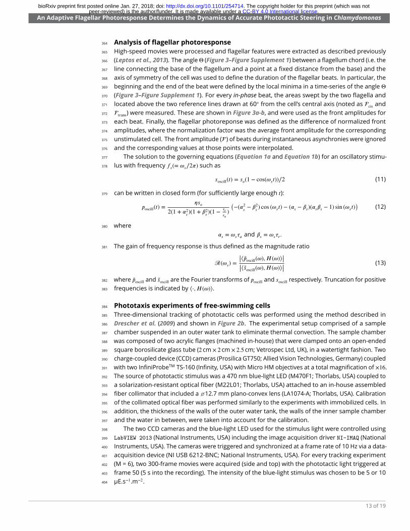
Figure 3–Figure supplement 1. Angle used to de�ne the beginning and the end of a beat. Achord is drawn from the base of each �agellum to a point of �xed length on the �agellum. Theangles ⇥cis and ⇥trans between each of the chords (red for cis and blue for trans respectively) and theaxis of symmetry of the cell (green), were used to de�ne the duration of the �agellar beats. Scalebar is 5�m.
670
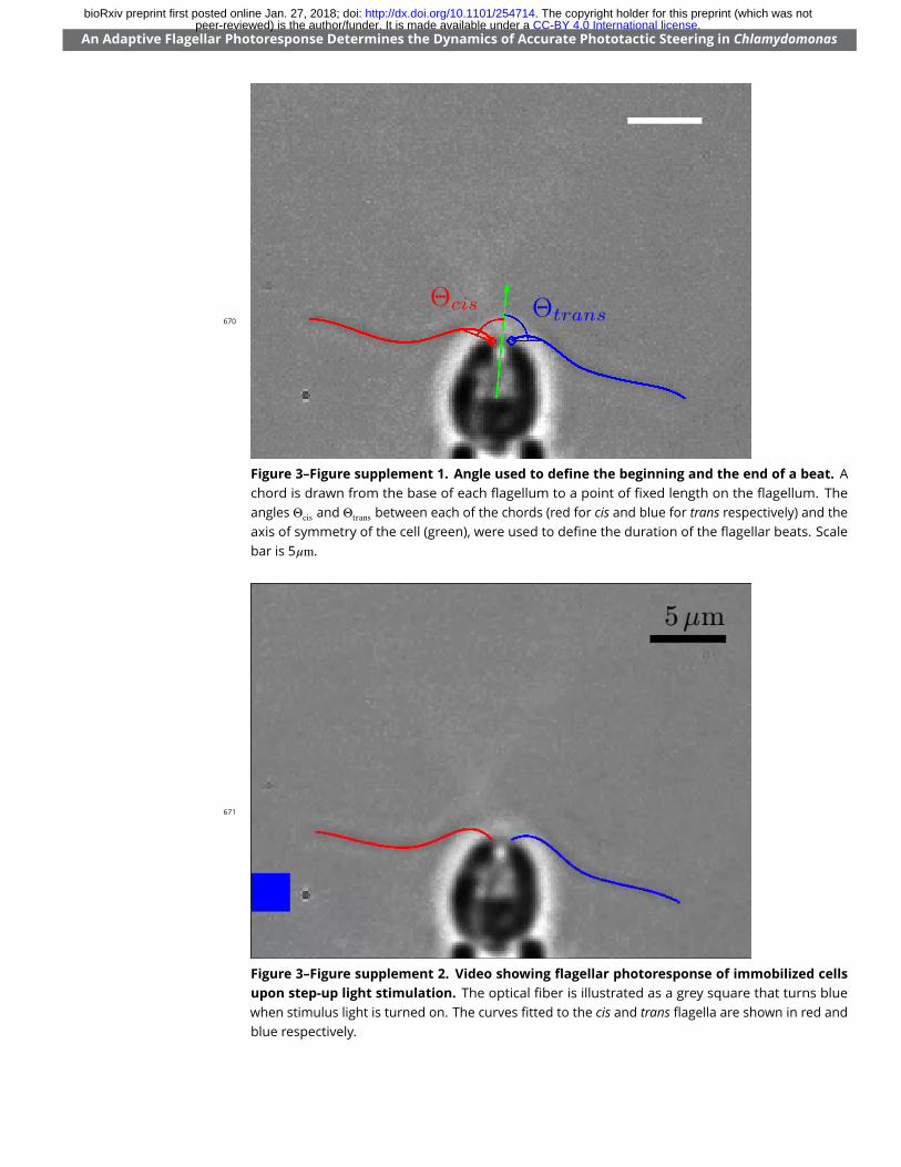
Figure 3–Figure supplement 2. Video showing �agellar photoresponse of immobilized cellsupon step-up light stimulation. The optical �ber is illustrated as a grey square that turns bluewhen stimulus light is turned on. The curves �tted to the cis and trans �agella are shown in red andblue respectively.
671
.CC-BY 4.0 International licensepeer-reviewed) is the author/funder. It is made available under aThe copyright holder for this preprint (which was not. http://dx.doi.org/10.1101/254714doi: bioRxiv preprint first posted online Jan. 27, 2018;
An Adaptive Flagellar Photoresponse Determines the Dynamics of Accurate Phototactic Steering in Chlamydomonas
-1 0 1 2Time (s)
01
PFD (μE.s -1.m
-2)
30
40
50
60
70
Inst
anta
neou
s be
atfr
eque
ncy
(Hz)
Figure 3–Figure supplement 3. Beat frequency �agellar photoresponse. The beat frequencyresponse for the same cell as shown in Figure 3c averaged over ntech = 4 movies. The instantaneousbeat frequency was calculated for each beat, ignoring beats that were out of synchrony. The meanand standard deviations of the instantaneous frequencies of the cis and trans �agella are shown inred and blue respectively.
672
.CC-BY 4.0 International licensepeer-reviewed) is the author/funder. It is made available under aThe copyright holder for this preprint (which was not. http://dx.doi.org/10.1101/254714doi: bioRxiv preprint first posted online Jan. 27, 2018;
An Adaptive Flagellar Photoresponse Determines the Dynamics of Accurate Phototactic Steering in Chlamydomonas
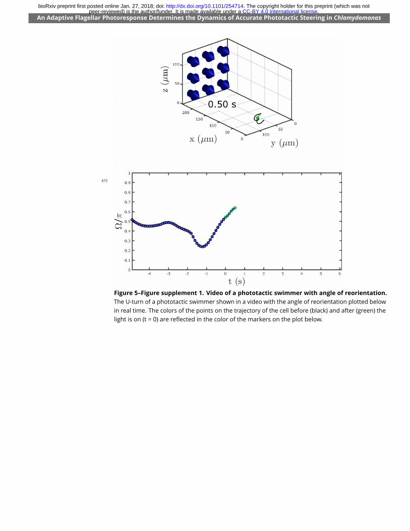
Figure 5–Figure supplement 1. Video of a phototactic swimmer with angle of reorientation.The U-turn of a phototactic swimmer shown in a video with the angle of reorientation plotted belowin real time. The colors of the points on the trajectory of the cell before (black) and after (green) thelight is on (t = 0) are re�ected in the color of the markers on the plot below.
673
.CC-BY 4.0 International licensepeer-reviewed) is the author/funder. It is made available under aThe copyright holder for this preprint (which was not. http://dx.doi.org/10.1101/254714doi: bioRxiv preprint first posted online Jan. 27, 2018;
An Adaptive Flagellar Photoresponse Determines the Dynamics of Accurate Phototactic Steering in Chlamydomonas
0(fitted)
1
2
3
0
1
2
3
(optimal)Freq
uenc
y (H
z)
Freq
uenc
y (H
z)
(fitted)(fitted) (Hz)
(opt
imal
) (H
z)
Reo
rien
t. (
s-1)
(a) (b)
(c) (d)
0
5
10
15
0
1
2
3
0 1 2 3
Figure 5–Figure supplement 2. Fitting parameter statistics. (a) Distribution of the �tted rota-tional frequency with median = 1.78 Hz (n = 21). (b) Distribution of the optimal rotational frequency,as de�ned by Equation 3 and using the �tted ⌧r and ⌧a pairs as shown in Figure 5c, with median =1.61 Hz (n = 21). (c) Linear correlation between �tted fr (from (a)) and optimal fr (from (b)), shown asa �tted straight line (blue) of the form f opt
r = 0.62f f itr +0.52. (d) Distribution of the �tted reorientation
constant � with median = 8.98 s*1 (n = 21).
674
.CC-BY 4.0 International licensepeer-reviewed) is the author/funder. It is made available under aThe copyright holder for this preprint (which was not. http://dx.doi.org/10.1101/254714doi: bioRxiv preprint first posted online Jan. 27, 2018;


![Torque Generated by Flagellar Motorof Escherichia - DAMTP · TorqueGenerated bythe Flagellar Motorof Escherichiacoil ... TES,N-tris[hydroxymethyl]methyl-2-aminoethanesulfonic acid.](https://static.documents.pub/doc/80x56/5c90c4f509d3f2c8148bd888/torque-generated-by-flagellar-motorof-escherichia-torquegenerated-bythe-flagellar.jpg)
