An Adaptive Landscape Classification Procedure Using ...

An Adaptive Landscape Classification Procedure Using Geoinformatics and Artificial Neural Networks

DISSERTATION

André Michael Coleman

Submitted in part fulfillment of the requirements for the degree of Master of Science in Geographical Information Systems

Faculty of Earth and Life Sciences

Vrije Universiteit, Amsterdam The Netherlands

June, 2008

ii

iii

Abstract The Adaptive Landscape Classification Procedure (ALCP), which links the advanced

geospatial analysis capabilities of Geographic Information Systems (GISs) and

Artificial Neural Networks (ANNs) and particularly Self-Organizing Maps (SOMs), is

proposed as a method for establishing and reducing complex data relationships. Its

adaptive and evolutionary capability is evaluated for situations where varying types of

data can be combined to address different prediction and/or management needs

such as hydrologic response, water quality, aquatic habitat, groundwater recharge,

land use, instrumentation placement, and forecast scenarios. The research

presented here documents and presents favorable results of a procedure that aims to

be a powerful and flexible spatial data classifier that fuses the strengths of

geoinformatics and the intelligence of SOMs to provide data patterns and spatial

information for environmental managers and researchers.

This research shows how evaluation and analysis of spatial and/or temporal patterns

in the landscape can provide insight into complex ecological, hydrological, climatic,

and other natural and anthropogenic-influenced processes. Certainly, environmental

management and research within heterogeneous watersheds provide challenges for

consistent evaluation and understanding of system functions. For instance,

watersheds over a range of scales are likely to exhibit varying levels of diversity in

their characteristics of climate, hydrology, physiography, ecology, and anthropogenic

influence. Furthermore, it has become evident that understanding and analyzing

these diverse systems can be difficult not only because of varying natural

characteristics, but also because of the availability, quality, and variability of spatial

and temporal data. Developments in geospatial technologies, however, are providing

a wide range of relevant data, and in many cases, at a high temporal and spatial

resolution. Such data resources can take the form of high-dimensional data arrays,

which can difficult to fully use. Establishing relationships among high-dimensional

datasets through neurocomputing based patterning methods can help 1) resolve

large volumes of data into a meaningful form; 2) provide an approach for inferring

landscape processes in areas that have limited data available but that exhibit similar

landscape characteristics; and 3) discover the value of individual variables or groups

of variables that contribute to specific processes in the landscape.

Table of Contents 1.0 Introduction........................................................................................................1

1.1 Problem Description ......................................................................................2 1.2 Research Objectives.......................................................................................4 1.3 The Adaptive Landscape Classification Procedure .......................................4 1.4 Report Contents and Organization.................................................................6

2.0 Landscape Classification and Modeling ............................................................8 2.1 Purpose of Landscape Classification .............................................................8 2.2 Current Methods of Landscape Classification.............................................11

2.2.1 Non-Statistical Approaches .................................................................11 2.2.2 Statistical Models.................................................................................13 2.2.3 Maximum Likelihood Classifier ..........................................................15 2.2.4 Multivariate Regression.......................................................................16 2.2.5 k-means ................................................................................................17 2.2.6 Ward’s Hierarchical Clustering ...........................................................20 2.2.7 Artificial Neural Networks ..................................................................22

3.0 Artificial Neural Networks ..............................................................................24 3.1 Pattern Recognition......................................................................................24 3.2 Soft Computing............................................................................................26 3.3 Fundamental Basis of Artificial Neural Networks.......................................26 3.4 Common Types of Artificial Neural Networks ...........................................32

3.4.1 Supervised Artificial Neural Networks................................................32 3.4.2 Unsupervised Artificial Neural Networks ...........................................35

4.0 The Adaptive Landscape Classification Procedure .........................................46 4.1 Purpose and Background .............................................................................46 4.2 The Components and Structure of the ALCP ..............................................48 4.3 Source Data Elements ..................................................................................50

4.3.1 Continuous Data...................................................................................50 4.3.2 Categorical Data...................................................................................54 4.3.3 Discrete Data........................................................................................55 4.3.4 Spatio-Temporal Data..........................................................................56

4.4 Geospatial Processing ..................................................................................58 4.4.1 Spatial Container..................................................................................58 4.4.2 SOM Pre-Processor..............................................................................62

4.5 SOM Model and Post-Processor..................................................................63 4.6 Visualization and Analysis ..........................................................................66

5.0 Application of the ALCP .................................................................................68 5.1 Multi-Spectral Classification .......................................................................68 5.2 30-Year Annual Mean Climatology.............................................................72 5.3 Hydrologic Properties and Landscape Characteristics ................................78

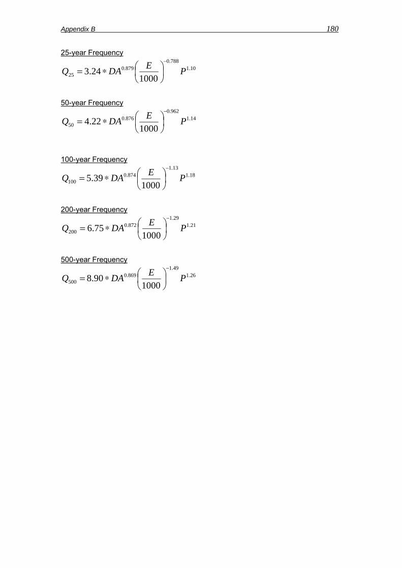
5.3.1 Flow Exceedence Analysis ..................................................................80 5.3.2 Flood Frequency Analysis ...................................................................85 5.3.3 Landscape Characteristics Analysis to Determine Hydrologic Properties .............................................................................................................91

6.0 Conclusions......................................................................................................98 6.1 Conclusion of Research Objectives .............................................................98 6.2 Limitations of the ALCP............................................................................100 6.3 Future Development Considerations..........................................................103

7.0 References......................................................................................................107

iv

8.0 Appendix A....................................................................................................120 9.0 Appendix B ....................................................................................................178

v

List of Figures

Figure 2.1. The basic process of classification groups univariate or multivariate input data similar or near-similar data into groupings based on a set of rules......................9

Figure 2.2. An example of an observationally interpreted landscape classification using variables of geology, physiography, vegetation, climate, soils, land use, wildlife distributions, and hydrology (Thorson et al., 2003). ...................................................12

Figure 2.3. Hierarchical approach to landscape classification where elements operating at broad temporal and spatial scale have more dominance over system processes (adapted from Snelder and Biggs 2002)...................................................13

Figure 2.4. A sample of 8000 points in the initial phase of k-means processing with random starting “seeds” placed in the input data space (a) and the final convergence stage (b). The cluster center, , is indicated by the large colored dot and parameter k=5 resulting in five distinctive cluster areas (Pelleg, 2004). .....................................18

jc

Figure 2.5. The ISOCluster model incorporates k-means, ISODATA, and the Maximum Likelihood Classifier, to organize and classify multivariate data................19

Figure 2.6. An example of the agglomerative hierarchical clustering for dominance of tree species in Wisconsin, USA (Bolliger et al., 2004). ..............................................22

Figure 3.1. This illustration exemplifies an anomaly (far right) in a regular pattern space. The mind immediately picks up on the abnormality, which thus becomes a point of interest (SFCC, 2007). ..................................................................................25

Figure 3.2. This set of objects relates the brains’ natural ability to recognize patterns and fill in missing information. Note the only objects that actually exist in this illustration are four incomplete circles with varying amounts of missing information. Through pattern-recognition, four complete circles and a square are comprehensible (SFCC, 2007). ............................................................................................................25

Figure 3.3. This illustration exemplifies the concept of proximity where the pattern on the left is viewed as a series of separate objects, the one in the middle is viewed as a single object (although it consists of separate objects), and the one on the right is viewed holistically as a single complex object composed of similar objects with different orientations (SFCC, 2007). ..........................................................................25

Figure 3.4. A simplified graphic representation of a neuron cell processing and transmitting information from cell to cell (adapted from Lingireddy and Brion, 2005)....................................................................................................................................27

Figure 3.5. A common and simple ANN schematic that represents the flow of information from the input data, to the receipt of the input neurons, to weighting and

vi

evaluating of data, to signal adjustments in the hidden layer, and finally the resulting output data (adapted from Principe et al., 2000)........................................................28

Figure 3.6. Result of a simple multi-layer perceptron ANN evaluating the MSE over model iterations. Once a sufficient MSE is reached, the optimal solution is obtained, meaning ANN output values closely match the training values and an underlying relationship has been established between input data vectors and resulting output. 31

Figure 3.7. A representation of the single-layer Self-Organizing Map process as it presents data to the network, competes, and maps organized data clusters to a defined 1-D, 2-D, or 3-D topology. .............................................................................38

Figure 3.8. A representation of the random weight initialization that occurs in the first phase of the SOM learning process. Input codebook vectors are presented to the randomly weighted neurons and the organization and learning process begins. ......39

Figure 3.9. A Gaussian function is often applied to a time-decaying kernel neighborhood to update the “winning” neuron and those in the effective area. This process makes the SOM learning efficient and stable. The kernel is defined by the center point and the kernel neighborhood is represented by the red rings, which become smaller with each time-step..........................................................................40

Figure 3.10. The SOM process captured at multiple iterations reveals the competition, learning, and projection of neurons over the input data space. Note that with an increase in iterations, the decaying kernel neighborhood function has less influence on the overall network structure and focuses on the learning and competition with individual neurons and their immediate neighbors. .........................42

Figure 3.11. A randomly generated 450x300 RGB image with 135,000 values used as input to a SOM training process. ...........................................................................43

Figure 3.12. The random initialization of neuron weights in a 2-D grid is presented. Each pixel in the grid is representative of a single neuron.........................................43

Figure 3.13. The final result of the SOM training from a 450x300 dataset reduced and organized into a 64x64 grid........................................................................................44

Figure 3.14. A 32x32 2-D trained SOM using the randomly generated source data presented in Figure 3.11. ...........................................................................................45

Figure 4.1. Four variables for 10 sub-basin areas are presented to illustrate different data patterns in the landscape. ..................................................................................47

Figure 4.2. An overview of the structure and flow of the ALCP.................................49

Figure 4.3. Two examples of continuous datasets that are raster-based and characterized by smooth transitions between the attributes. .....................................51

vii

Figure 4.4. Categorical data comprise a dataset classified by pre-defined groupings as presented in the two examples..............................................................................55

Figure 4.5. Spatio-temporal data representing a 1-day maximum temperature forecast condition from the National Digital Forecast Database (NDFD) meteorology model (NWS, 2007)....................................................................................................57

Figure 4.6. A spatio-temporal dataset representing snow-water equivalent conditions for a given day. New data results are produced daily from the United States National Oceanic and Atmospheric Administration’s Snow Data Assimilation Model (SNODAS) (NOHRSC, 2007). ......................................................................................................57

Figure 4.7. The sub-watersheds presented in this figure serve as a spatial container for data harvesting and compilation of data exhibiting multiple-scales and data types....................................................................................................................................60

Figure 4.8. The basic process flow and function of the spatial container (as represented by sub-watersheds) within the ALCP. The input neurons are representative of the vector codebook patterns containing the multiple datasets that are used in the classification. .....................................................................................61

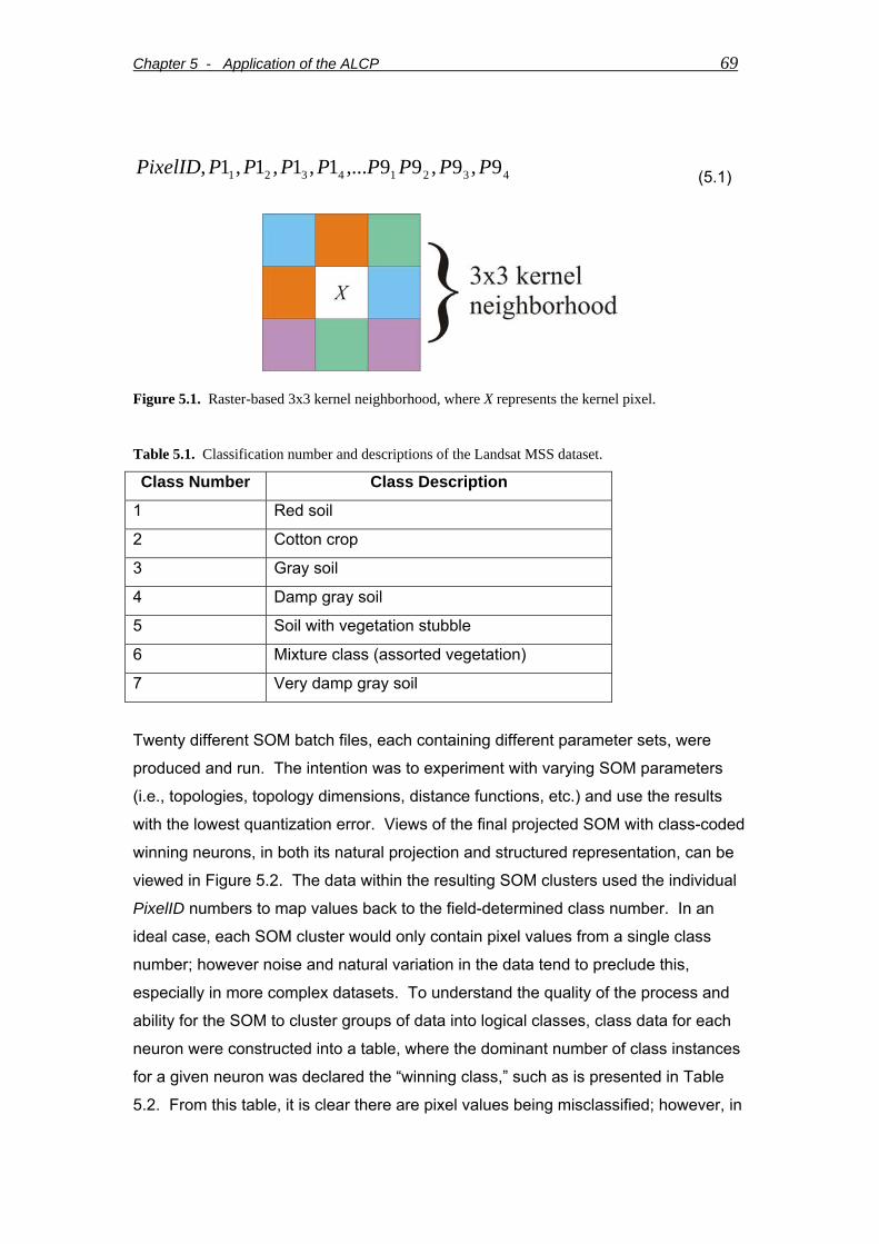
Figure 5.1. Raster-based 3x3 kernel neighborhood, where X represents the kernel pixel............................................................................................................................69

Figure 5.2. The upper four figures display the Landsat MSS input data space (represented by class-colored cubes) and the final projected SOM neurons (represented by class-colored spheres). The bottom two figures display the final projected SOM in structured space............................................................................71

Figure 5.3. An overview of the 3075 ALCP spatial containers used for analysis on the North Fork of the Clearwater River watershed.....................................................72

Figure 5.4. The input data space (colored cubes) and random-weighted neurons (spheres) for the North Fork Clearwater three-parameter climate data are represented in (a). The final projected SOM, a three-dimensional 2x2x2 cubic topology network, is presented in (b). ........................................................................74

Figure 5.5. The ALCP analysis/spatial classification of 30-year annual mean climate data in the North Fork of the Clearwater watershed. Existing meteorology stations are noted with the red triangles..................................................................................74

Figure 5.6. Linear regression analysis evaluating the relationship of elevation to precipitation, maximum temperature, and minimum temperature..............................76

Figure 5.7. Box-and-whisker plots for precipitation minimum temperature and maximum temperature for each SOM-determined cluster. ........................................77

Figure 5.8. Bar graph representing the total area occupied by each SOM-clustered class as represented in Figure 5.5. Note that existing meteorology collection stations exist in Class 2, Class 6, and Class 8. .......................................................................78

viii

Figure 5.9. A total of 160 headwater catchments were derived for hydrologic and landscape analysis. The selected basins represent approximately 63% of the total watershed area. .........................................................................................................79

Figure 5.10. Area distribution of the 160 sub-basins sampled for analysis...............80

Figure 5.11. Monthly values of 80% flow exceedence for all 160 test sub-basins. Flow units are in cubic feet per second (cfs)..............................................................82

Figure 5.12. Monthly values of 20% flow exceedence for all 160 test sub-basins. Flow units are in cubic feet per second (cfs)..............................................................82

Figure 5.13. Final SOM projection for (a) Q80 and (b) Q20......................................83

Figure 5.14. Mean values of each SOM cluster per month for (a) Q80 and (b) Q20....................................................................................................................................84

Figure 5.15. Spatial mapping of the Q80 and Q20 SOM cluster results. The classes are sorted based on flow with Class 1 being the lowest and Class 8 the highest......85

Figure 5.16. Flood frequency values representing both flood magnitude and return period for each of the test basins. ..............................................................................87

Figure 5.17. Mean cluster values per return period for flood frequency analysis......88

Figure 5.18. SOM classification of flood frequency data for three return intervals over 160 sub-basins...........................................................................................................89

Figure 5.19. Linear regression plots testing the relationship of sub-basin area to flow magnitude for 2-, 10-, 100-, and 500-year return periods. .........................................89

Figure 5.20. 100-year flood frequency regression plot with point members symbolized by their assigned SOM cluster. ...............................................................90

Figure 5.21. Spatial mapping of the nine-period flood-frequency SOM cluster results. The classes are sorted based on mean flow values within each cluster, where Class 1 represents the lowest flows and Class 8 the highest. .............................................91

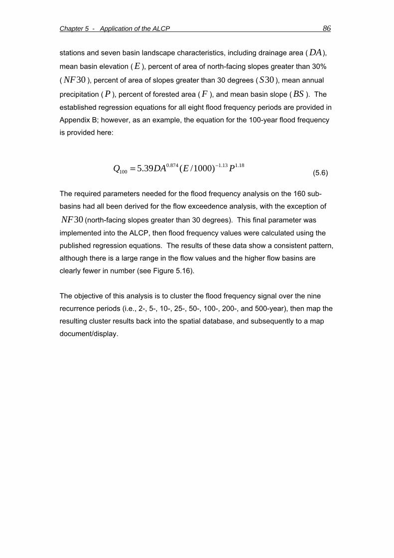
Figure 5.22. The input data space (colored cubes) and final projected neurons (spheres) in (a) natural projection space and (b) structured representation. The final SOM structures represent the clustering of 10 landscape metrics. Note that one neuron, best viewed in (b), was not used, indicating a sufficient number of neurons used. ..........................................................................................................................93

Figure 5.23. Bar graphs indicating (a) the overall similarity in the landscape and Q20 class boundaries, and (b) the degree of class change for those basins that were identified as being dissimilar. .....................................................................................94

ix

Figure 5.24. Similarity index map showing likeness and difference between two independent cluster analyses, using 1) spatial landscape metrics, and 2) Q20 regression equations and landscape metric data to feed the regression equations. .95

Figure 6.1. A design concept for a hybrid ANN model combining the unsupervised SOM classification with a supervised ANN such as the Multi-Layer Perceptron, resulting in a supervised classification of spatial data..............................................102

Figure 6.2. The concept of SOM Attribute Weighting is presented as a potential method for assigning data theme weights is the classification process. ..................105

x

List of Tables Table 3.1. Common activation functions used in ANN models (StatSoft, 2003). ......30

Table 3.2. A small sample of Fisher's multivariate Iris flower dataset (Fisher, 1936)....................................................................................................................................33

Table 4.1. Terrain-based data processed and extracted within the ALCP................51

Table 5.1. Classification number and descriptions of the Landsat MSS dataset. .....69

Table 5.2. Class-assigned pixel counts for each SOM neuron are presented. The dominant count value, marked in bold-italic typeface, is declared the “class winner” for the neuron.............................................................................................................70

Table 5.3. A confusion matrix showing classified and misclassified data by class. Values indicated by bold-italic typeface indicate correctly classified values. All data are presented as percentages. ..................................................................................70

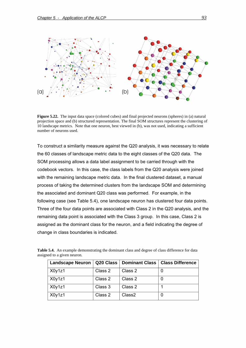
Table 5.4. An example demonstrating the dominant class and degree of class difference for data assigned to a given neuron. .........................................................93

Table 5.5. Source spatial data the USGS used to support and develop multivariate regression equations (left), and the data source used in the landscape analysis test (right)..........................................................................................................................96

xi

Disclaimer The results presented in this thesis are based on my own research at the Faculty of Earth and Life Sciences of the Vrije Universiteit Amsterdam. All assistance received from other individuals and organizations has been acknowledged and full reference is made to all published and unpublished sources. This thesis has not been submitted previously for a degree at any institution. Signed: ___________________________________ Date: ___________________________________

xii

Acknowledgements First and foremost, my gratitude and love are expressed to my wife, Laurie, and my

children, Isabella and Sophia, for the countless hours I have spent fulfilling a desire

to increase my knowledge in the sciences of geography, geographic information, and

hydrology. My ultimate purpose in this effort is for no other reason than to help gain

a better understanding of the beauties and complexities that lie in our natural world.

I would also like to express my appreciation for the love and support given to me by

my greater family. Your words and actions throughout my studies have given me

much needed strength.

None of this research would have been possible without my friend and mentor Lance

W. Vail, whom repeatedly planted the seed sprouting the growth of this research.

While it took some three years just to conceptualize what this seed was and its

potential fruits, I’m grateful for the introduction to the crazy and amazing world of

machine learning and neural networks.

My appreciation and gratitude are extended to my advisor, Professor Andrea Fabbri,

whom graciously accepted the offer to supervise me through this process. Despite

my trepidation after our first meeting (the questions you posed to me at this time left

me thinking for two months!), I am indebted to you for your knowledge, thought-

provoking insights, and prompting me to seek real meaning behind words commonly

misused.

Lastly, I wish to acknowledge and thank the UNIGIS program director, Professor

Henk Scholten, and the rest of the quality instructors and staff involved in the UNIGIS

Amsterdam program. With this year being the 15th anniversary of the program, this is

a significant occasion and speaks very favorably to all the people who contribute to

the success of the program. This has truly been an uplifting and rewarding

experience providing a unique international perspective into the field of Geographic

Information Sciences.

I am indebted to and humbled by all of you. With my deepest regards, André M. Coleman May, 2008

xiii

Acronyms AI Artificial Intelligence ALCP Adaptive Landscape Classification Procedure AML Arc Macro Language ANN Artificial Neural Network ART Adaptive Resonance Theory (network) CVS Concurrent Versions System DEM Digital Elevation Model DNA deoxyribonucleic acid GIS Geographic Information System GISc Geographic Information Science GLCP Global Land Cover Characterization Program JDEVS Java Discrete Events System LVQ Learning Vector Quantization MLC Maximum Likelihood Classifier MLP Multi-Layer Perceptron MSE Mean Square Error MSS Multi-Spectral Scanner NASA National Aeronautics and Space Administration NDFD National Digital Forecast Database NDVI Normalized Difference Vegetation Index NED-H National Elevation Dataset Hydrologic Derivatives NLCD National Land Cover Database PCA Principal Component Analysis pdf Probability Distribution Function PNN Probabilistic Neural Network PRISM Parameter-elevation Regressions on Independent Slopes Model Q20 20% Flow Exceedence Q80 80% Flow Exceedence RBF Radial Basis Function (network) RGB Red Green Blue (color scheme) RNN Recurrent Neural Network SAGA System for an Automated Geographical Analysis SDM Spatial Data Modeler SOM Self-Organizing Map SRTM Shuttle Radar Topography Mission SVM Support Vector Machine USACE United States Army Corps of Engineers USGS United States Geological Survey

xiv

xv

Chapter 1 - Introduction 1

1.0 Introduction Environmental management and research across a heterogeneous landscape

provides challenges for consistent evaluation and understanding of natural

processes. A heterogeneous landscape can exist in a wide variety of forms ranging

from differences in specific hydrologic processes such as streamflow, groundwater

recharge, rates of erosion or different ecological phenomena including biotic

diversity, patch densities, and community dynamics. The magnitude of heterogeneity

is variable and subject to the domain of study. For instance, an evaluation of stream

temperatures for the purpose of understanding water quality and fish survival issues

may present a limited domain of stream temperatures that are possible within the

area of study. The classification of heterogeneous landscapes offers the ability to

better understand individual or collective variables that contribute to natural

processes and responses in the landscape.

The classification of landscapes over large spatial domains can present unique

challenges due to the availability and diversity of data. With the exception of

designated and protected research areas throughout the world, such as experimental

watersheds and forests, detailed data collections are often limited to small areas with

a specific research focus, largely due to the expense of carrying out large-scale

research studies. While advances in automated data collection methods including

space-based sensor platforms and field instrumentation have dramatically increased

in their availability and reliability in the past three decades, there still remains a

fundamental issue of retrieving sufficient information on the ground to develop a

relationship between sensor and ground conditions; this step is vital to effectively

make use of data across the entire landscape. For example, a meteorology

instrument station collects weather information for one specific location in space and

thus knowledge in between this station and others have a large degree of

uncertainty. Similarly for space-based sensors, without an on-the-ground study,

there is no way to relate spectral signatures to real elements in the landscape.

The research presented here identifies a procedure, showing positive results, that

provides a powerful and adaptive procedure capable of processing large volumes of

complex data, discovering relationships and patterns in the data, and reducing the

data complexity to a more meaningful form by classifying common data patterns.

The developed procedures can be used to propagate detailed information learned

from a given spatial domain to other areas in the landscape without the same level of


detailed information. This notion, among other things, allows for the intelligent and

efficient pre-planning of research and monitoring studies to effectively capture the

unique aspects in the landscape, and then apply the learned information to the “data

gaps” or areas in between the specific study sites. The procedure is well suited for

use in adaptive environmental modeling, research, monitoring, and management, as

well as predictive and solution capabilities for a wide range of topic areas (i.e.,

determine probable locations of groundwater recharge zones, ideal restoration and/or

protection areas, field sampling and instrument location sites, land use assessment,

“what-if” scenarios for various environmental impacts, etc.) and is specifically

intended to be adaptive in the types of data that can be used and the problem sets it

can be used for (i.e., not necessarily limited to addressing landscape-based

questions).

1.1 Problem Description

The fundamental problem this research attempts to address is whether or not it is

possible to have rich knowledge in a given domain of space and time in the

landscape and convey this knowledge to other areas in the landscape that exhibit

limited knowledge, yet possess some similar properties. The implications of finding

an answer to this question can be significant in terms of understanding landscape

processes at a finer scale, which enhances our ability to monitor and manage these

landscapes. For example, the United States Geological Survey (USGS) currently

maintains a nationwide network of approximately 8,900 gages to monitor streamflow.

Each year, because of budget constraints, many of these gages are permanently

taken out of service. The impact of using known and measured streamflow

information along with other metrics defining the landscape, and propagating this

information to other areas without stream gages could lead to efficient use of

available funds by prioritizing the value of a gage in terms of the uniqueness of the

watershed it represents, and thus making informed decisions when removing gages.

Additionally, the USGS currently relies on multivariate regression formulas built from

20+ years of measured data to estimate streamflow characteristics in watersheds

without instrument data. With anticipated changes in climate, particularly in mountain

environments, regression formulas may be of less value since past data records may

not be indicative of future conditions. The same concept as described for USGS

stream gage data can be brought forth to assist in propagating knowledge across the


landscape for various in situ data collection such as stream temperature, rates of

erosion, groundwater recharge, and wildland fire potential.

Evaluation and analysis of spatial and temporal patterns in the landscape can

provide knowledge and understanding of complex ecological and hydrological

processes. Landscape patterns are not random, rather a structure underlies their

variability. The patterns are driven and developed by a complex array of abiotic and

biotic factors such as topography, climate, macroclimate, soils, ecosystem function,

and anthropogenic influence (Turner et al., 2003). The spatial patterns of various

elements in the landscape have a direct relationship with the processes in the

landscape. The use of geoinformatics and Artificial Neural Networks (ANNs),

particularly Self-Organizing Maps (SOMs), is proposed as a method to discover

patterns in the landscape and system functions between areas in the landscape that

are not only spatially disjointed, but dissimilar in their available data.

The use of ANNs is well-established in many sciences including genomics, risk

analysis, forecasting, artificial intelligence, medicine/biomedicines, and more.

Although a review of literature indicates both successes and failures using ANNs, the

reviews of the successful applications show what is possible. As stated by

Govindaraju and Rao (2000), “Researchers claim to be drawn to artificial neural

networks because they possess desirable attributes of universal approximation,

ability to learn from examples without the need for explicit physics, and the capability

of processing large volumes of data at high speeds.” The use of ANNs appears to be

effective for understanding complex datasets and in the field of remote-sensing,

these methods have proved themselves in the realm of research and are now

emerging into commercial applications. From a review of the literature, it is clear the

use of ANNs in Geographic Information Science (GISc) is still quite limited, even in

the research domain.

The specific problems being addressed in this research are to:

• resolve and provide meaning to large amounts of spatial data that exist at

different scales and come from different sources.

• explore the value of ANN models within the realm of GISc to discover

similarities in complex data patterns and infer landscape processes in areas

that have limited data available but exhibit similar landscape characteristics.


• discover the value of individual variables or groups of variables that contribute

to specific processes in the landscape.

1.2 Research Objectives

The goal of the study reported here is to research and integrate geospatial

processing methodologies using ANNs, particularly SOMs, to develop an adaptive

procedure for landscape classification that can be used in a heterogeneous

environment of data, data availability, standards, quality, resolution, management,

ecology, physiography, and climate to gain a higher-level understanding of landscape

processes, so that existing knowledge can be propagated to other domains. The

strengths of ANNs, in general, is that they allow for the development of complex,

high-dimensional datasets that are distribution free and can handle nonlinear data

structures. The procedures developed in and for this research attempt to overcome

the problem of using diverse and complex datasets. The Adaptive Landscape

Classification Procedure aims to identify nonlinear landscape patterns from a set of

high-dimensional spatial data, including terrain morphometry, hydrology, vegetation,

land use, soils, and climate, at a variety of spatial and temporal scales.

The specific objectives of this research are as follows:

1) Demonstrate the capability to transfer knowledge from one area or aspect

of the landscape to another where knowledge is limited.

2) Improve understanding and linkages between ANNs and geoinformatics.

3) Develop a method for handling diverse and complex data in a spatial

environment and provide an alternative method to traditionally used

classification methods.

1.3 The Adaptive Landscape Classification Procedure Automated data collection methods have dramatically increased with advances in

technology over the past three decades. Despite these advances, it remains difficult

and expensive to monitor and understand all aspects of a natural system. Outside of

designated research areas such as the H.J. Andrews experimental forest in Oregon,

USA or the Dragonja River experimental watershed in Slovania (Sraj et al., 2006),

intensive data collection and research are typically focused on small geographical


areas with a specific focus, such as stream habitat restoration or evaluation of plant

community succession. A procedure developed in this research, the Adaptive

Landscape Classification Procedure (ALCP), uses available and known spatial and

temporal information within a given landscape to establish data patterns and clusters

where there are similarities in the data characteristics. The type of data and the

magnitude at which the ALCP is used, depends on the area of focus. For instance,

clusters of data can be established within a watershed to strictly determine where

similar geomorphic characteristics exist. Using a wide array of terrain-based metrics,

the ALCP can produce a complex high-dimensional dataset, reduce it to a low-

dimension, and determine data similarities using Self-Organizing Maps (SOMs)

clustering. The results are useful for understanding hydrologic processes related to

terrain, determining the potential for mass-wasting (i.e., landslides), or understanding

the sediment transport potential within a watershed. The ALCP also can help

determine where to focus site monitoring and/or instrumentation and restoration

activities, evaluate the spatio-temporal effects found in inter-annual seasonal

variations or long-term climate change, and provide a predictive capability for biotic

variables in the landscape. The results of several case studies conducted during this

research are reported.

The use of ANNs provides the core capability in the ALCP. The literature suggest

that the use of ANNs in the natural sciences has been steadily applied in the past

decade, including a number of studies that also integrate Geographic Information

System (GIS) capabilities to strengthen the overall process and provide meaningful

results (Bacao et al., 2005a; Bryan, 2006; Catani et al., 2005; Dai et al., 2005; Ermini

et al., 2005; Hilbert and Ostendorf, 2001; Hsieh and Jourdan, 2006; Joy and Death,

2004; Wang and Sassa, 2006). ANNs are powerful tools that are well suited for

solving complex nonlinear classification problems because they enable the discovery

and development of previously unknown data inter-relationships and patterns. In

addition, ANNs offer “…an alternative to traditional statistical approaches for

predictive modeling when nonlinear patterns exist” (Joy and Death, 2004). The input

data for an ANN model can be nonlinear, categorically independent, multi-scaled,

incomplete, and have mixed-type parameters such as those that might be found in

soils, vegetation, hydrology, and terrain-based data (Catani et al., 2005; Dixon, 2005;

Hilbert and Ostendorf, 2001). When an ANN model is established using a wide array

of input data, it is well suited to being adapted to different scenarios that might be

found in different landscape environments. As is demonstrated by the research

documented in this report, the ALCP specifically deals with issues of multiple scales


by using a “spatial container” that captures input data within a defined boundary,

derives statistically descriptive metrics of the data, normalizes the data using

principal components analysis, and then delivers the results to the SOM for pattern

clustering.

1.4 Report Contents and Organization

The results of the research study are reported in the ensuing section of this report, as

follows:

• Chapter 2.0 describes the background and relevancy of landscape

classification and its importance across many disciplines. It discusses

various landscape classification approaches and models and reviews

commonly used statistical methods such as multivariate regression and k-

means.

• Chapter 3.0 provides information about ANNs, including some of their

capabilities, capacities, and varying model structures and their requirements.

Because many types of ANNs exist, each serving different purposes, gaining

a broad understanding of their characteristics provides perspective of the core

processor of the ALCP chosen for use in this research—the SOM.

• Chapter 4.0 gives a detailed account of the methodology, framework, and

mechanics of the ALCP including data requirements, data production

supporting multi-scaled, heterogeneous inputs, and software written to

support this research.

• Chapter 5.0 demonstrates and analyzes the ALCP on several test- and real-

world applications.

• Chapter 6.0 discusses research findings and conclusions and provides

recommendations for future research and development.

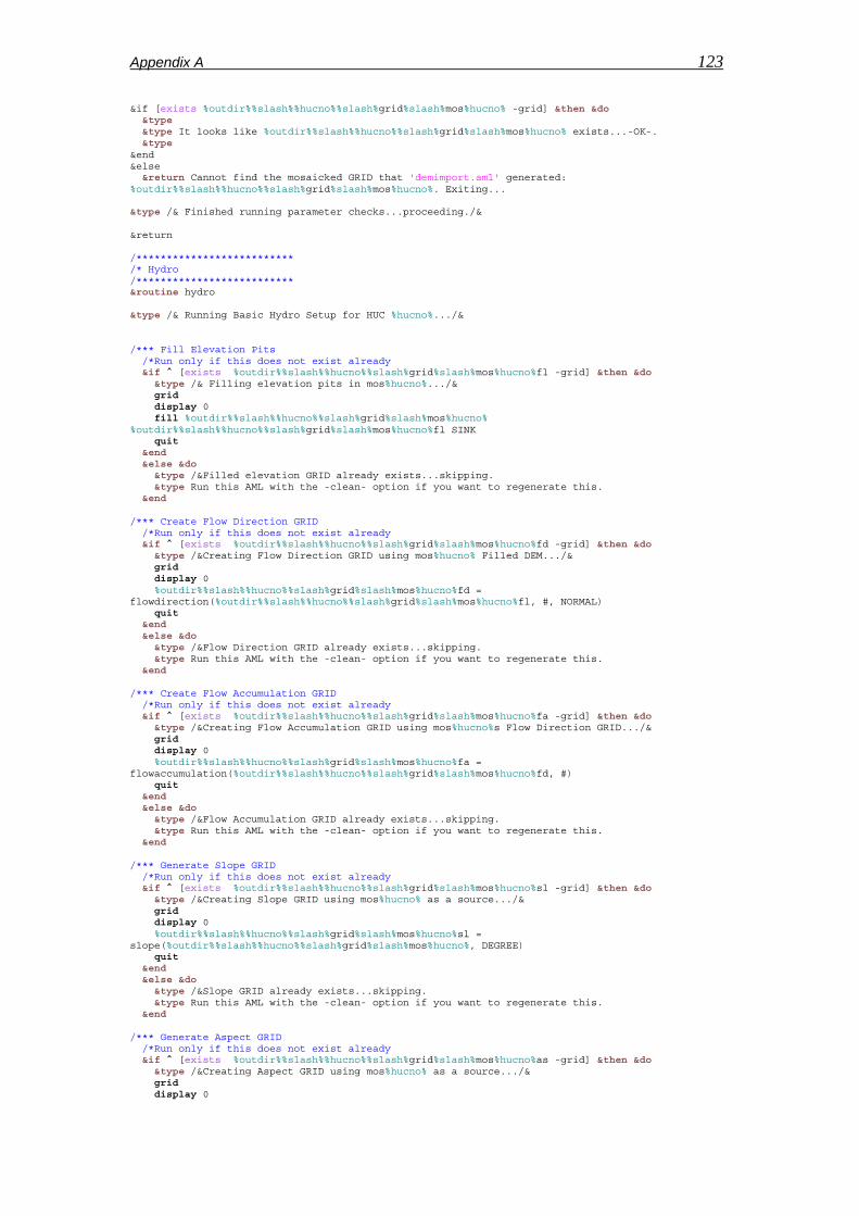
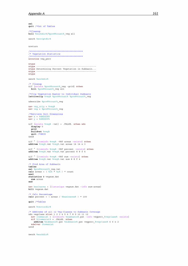
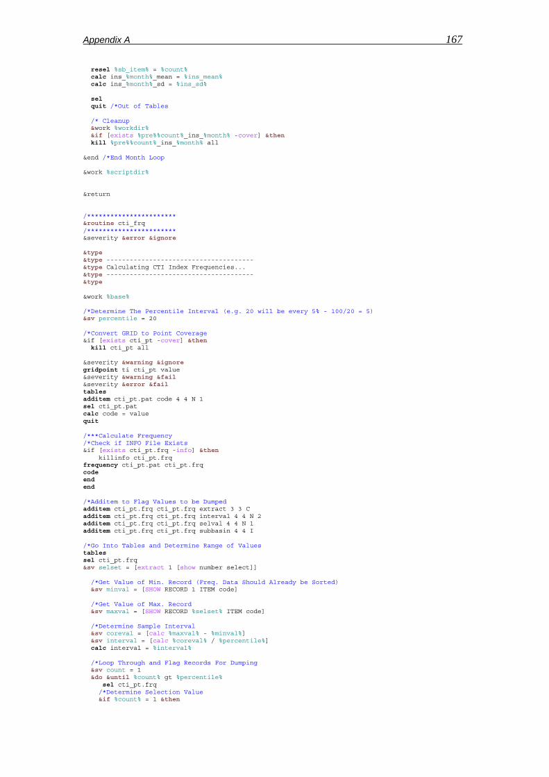
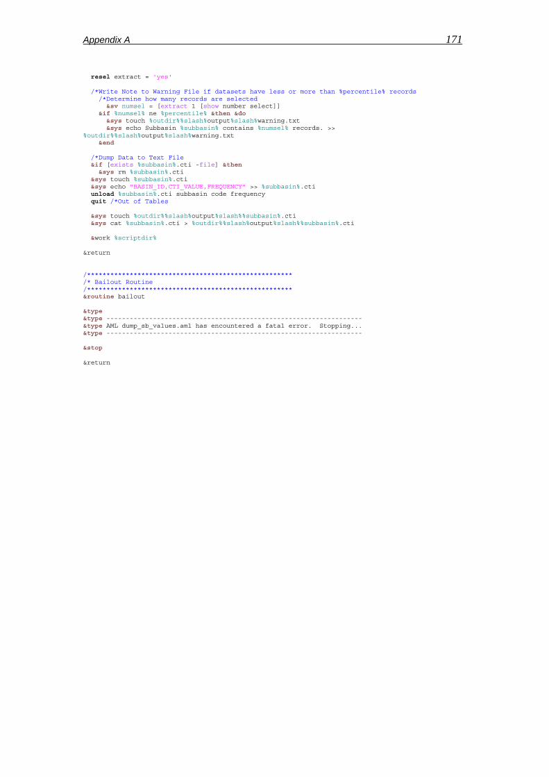
• Appendix A documents the primary software codes written to support the

ALCP.


• Appendix B provides a detailed listing of multivariate regression equations

used to develop streamflow patterns as analyzed in Chapter 5.0

Chapter 2 - Landscape Classification and Modeling 8

2.0 Landscape Classification and Modeling This chapter describes the purpose and current methods of landscape classification

including non-statistical methods, statistical models and Artificial Neural Networks.

The classification methods provided here are intended to give context to what is

commonly used and noted in current literature. This research does not attempt to

compare the various classification methods largely because these studies can be

found elsewhere (see Bacao et al., 2005b; Bryan, 2006; Gomes, 2007; Lin and Chen,

2006; Rao and Srinivas, 2008; Schmidt and Hewitt, 2004).

2.1 Purpose of Landscape Classification

Spatial and temporal processes have an explicit cause-and-effect relationship to

landscape patterns. These patterns can be detected by observation of biotic or

abiotic factors that have the power to influence ecological relationships, hydrological

functions, or other natural or anthropogenic-induced processes. A “landscape” is

fundamentally composed of a patchwork of possibly recognizable spatial units, which

could vary in extension and character depending on the variables used to identify

homogeneous areas; typically, these variables involve elevation, morphometry,

climate, vegetation, and soils (Bailey, 1995; Bailey, 2004; Turner, 1989). The notion

of landscape classification and the determination of homogeneous areas have been

important research issues for many disciplines including geography, ecology,

hydrology, watershed and water resource management, land-use planning and

policy, and environmental management. The multi-disciplinary need for regionalizing

the landscape, or dividing it into different domains, resulted in a variety of

classification methods and variables as different views were applied and consequent

requirements had to be met. Overall, conducting landscape classification is a difficult

task largely because of the fuzzy nature of natural-process boundaries and functions

and the multiple scales at which these boundaries and/or processes are observed.

In addition, it is difficult to capture or recognize hidden and/or unknown process

interactions. Clearly, the elements that are brought into a classification scheme can

range from very basic to highly complex, depending on the purpose and question(s)

being addressed. Regardless of the classification purpose, (e.g., landscape units,

species distribution, or demographics), the objective of classification is to reduce the

complexity and facilitate the interpretation of the real world by grouping similar

elements together and constructing a convenient abstraction from the original


observations. As depicted in Figure 2.1, a classification process, no matter which

method is used, sorts and organizes the input data space into a feature space with

some kind of logical ordering and grouping.

Figure 2.1. The basic process of classification groups univariate or multivariate input data similar or near-similar data into groupings based on a set of rules.

As humans, we have a natural tendency, through normal brain functions, to establish

patterns and associations in our environment. It is this ability of pattern recognition

that allows us to distinguish objects from one another, to interpret speech, and to

read—for instance, to provide meaning to the compilation of letters on this page.

Through casual observation, it appears to be relatively effortless to recognize and

define basic and homogeneous landscape patterns in our environment such as

forest, desert, alpine, grassland, etc. (Watts, 1971). These definitions of broad

landscape types introduce an association of further attributes that enhance and

unfold the characterization of the environment. For example, through personal

experience or knowledge obtained in some other capacity, one might conceive that a

desert landscape possesses certain basic characteristics, such as limited water

resources, large fluxes in temperature, a limited amount of flora and fauna, etc.

These broadly described attributes of the desert landscape have the capacity to

reveal new insights and develop relationships between elements within the

environment. For instance, because of the large temperature fluxes and limited

amount of water, the flora and fauna are dormant in the day and active at night to

conserve energy and water; there is a limited amount of vegetation due to a limited

amount of precipitation; the hardy structure and composition of desert flora are the

result of their protecting themselves in a landscape that has many environmental


extremes. While the previously described characterization of the desert environment

is a relatively simple task for the human mind to process, it is difficult to mimic this

type of pattern recognition in a computational context. In other words, how do you

get a computer to recognize the difference between a desert and a forest? The

importance and purpose of researching a computationally based pattern-recognition

and classification system drive the need for a consistent mechanism that is capable

of reducing observational data complexity (e.g., multi-spectral sensors; in situ

measurements of streamflow, soil moisture, evapotranspiration, and meteorology).

This complexity increases dramatically when considering the horizontal and vertical

dimensions of space, the time dimension, and a suite of varying observational data.

Forman (1986) describes structure, function, and change as three fundamental

characteristics of the landscape. Structure defines the spatial distribution of energy

and matter across the landscape, while function describes the interactions and

relationships of the spatially distributed energy and matter. Change is defined by any

alteration to the structure and/or function over time. The properties of temporal and

spatial dimensions in the landscape will have profound effects on understanding and

determining patterns and processes in the landscape. Consider, for example, how

the potential effects of climate change in the landscape may be evaluated at a time

resolution of ~5-30 years. They would most typically have an effect over a large

area, although how the various effects are revealed in the landscape could be

defined as a fine-scale problem (i.e., fine detail changes to plant communities and

successive change to the landscape ecology). Conversely, for a localized mass-

wasting event that is caused by a short-duration, high-magnitude precipitation event

and results in an immediate disturbance, landscape elements should be evaluated on

a fine temporal and spatial scale. However, the long-term effects of the mass-

wasting process can have implications over long temporal scales and large areas

depending on the sediment transport mechanisms in the landscape and where in the

landscape the process is distributed. Human perception of biotic and abiotic

processes in the landscape will affect our notion of scale and these perceptions will

contribute to the effects of collecting appropriate types and amounts of data to

interpret the landscape. These fundamental properties of the landscape provide a

basis for understanding the process complexities that exist within it. While it is

unlikely that the landscape and its dynamic interactions and processes will ever be

fully understood, the use of models to simulate natural processes can assist in

bringing complexities to a comprehensible level.


To evaluate process relationships in the landscape, elements need to be classified

over a range of observations, from the micro-scale to the regional-scale and beyond.

This type of approach allows for “neighborhood relationships and landscape position

in a higher-scale context” (Schmidt and Hewitt, 2004). For example, evaluating many

small individual areas for micro-topography elements may miss the bigger picture;

e.g., that what you are actually evaluating is an entire mountain. Multi-scaled

classification, through space and time, is an important step to reveal different

patterns.

2.2 Current Methods of Landscape Classification

The methods for classifying landscape currently include non-statistical approaches

and statistical models.

2.2.1 Non-Statistical Approaches

Traditionally, common and accepted practices in landscape classification have

involved direct observations and interpretations of landscape patterns (see Figure

2.2), which were frequently based upon biotic factors (Bailey, 2004; Bryan, 2006;

Lioubimtseva and Defourny, 1999; Osinski, 2003). While some approaches were

rather simple, abstracting the landscape for broad-area regionalization, other

approaches managed the complexity of the natural environment by using a

hierarchical approach in which patterns at multiple scales are assumed as controllers

of ecosystem functions (Bailey, 1995; Snelder and Biggs, 2002). For example, broad

elements of time and space, such as climate, will have the largest control over the

landscape having the power to affect water resources, soil composition, land cover,

etc. The hierarchical approach ranges from broad macro-processes to micro-

processes where each successive element has less control over the environmental

condition than the preceding element (Bailey, 2004; Snelder and Biggs, 2002) (see

Figure 2.3).

The advent of digital spatial data and GIS technology brought forth the gathering of a

multiple datasets where simple or complex integrating and weighting schemes were

established, thus revealing information in entirely new ways. For example, long-term

mean values of meteorology, vegetation, and soil types could all be assigned a


unique code based on their attributes. Then, using a raster data model, or a cell-

based matrix where each cell contains an attribute value and a position in space, the

various data could be combined to create a set of classifications based on the

arithmetic sum of the unique codes. These GIS-derived landscape patterns revealed

a more complex spatial representation than manually delineated classifications.

These new approaches were the beginning of using computational methods to reveal

complexities found in the natural environment. With increases of data availability and

spatial resolution came the potential for data errors. This was exemplified with data

produced using automated and/or semi-automated collection procedures such as

those used in the development of Digital Elevation Models (DEMs) (Russell, 1997). In

many cases, GIS approaches had to be supplemented with manual interpretation

and delineation of similar landscape types, integrating information from other

sources, such as field notes, existing classifications, or other types of information and

yielded hybrid approaches in the classification process.

Figure 2.2. An example of an observationally interpreted landscape classification using variables of geology, physiography, vegetation, climate, soils, land use, wildlife distributions, and hydrology (Thorson et al., 2003).


Figure 2.3. Hierarchical approach to landscape classification where elements operating at broad temporal and spatial scale have more dominance over system processes (adapted from Snelder and Biggs 2002).

2.2.2 Statistical Models

Statistical techniques have been a common theme in the arena of landscape

classification and particularly in the last two decades where they could be applied

more easily within a digital geospatial context. The advantages of using various

statistical methods helped to provide classifications with stronger bases and

quantitative significance with respect to manual interpretations, hierarchical classing,

and aggregation and/or weighting techniques. From a statistical point of view,

classification problems can be further broken down into three classes (Michie et al.,

1994): 1) classic statistical approaches such as linear discrimination and explicit

probabilities; 2) machine learning, which employs logic-based automated processing

that uses large amounts of data to train into interpretable classes; and 3) ANNs,

which mimic the unconscious side of brain function-solving relationships and are

incorporating statistical and machine learning methods. A common theme of any

classification is the need to apply an objective method for determining the class

boundaries. Statistical models such as multivariate regression, k-means, linear and


quadratic discriminate analysis, decision trees, and Bayesian networks are viewed in

current literature as being significant for obtaining or generating the classification of

data.

A basic clarification needs to be made here, to explain the difference between

“classification” and “clustering.” The terms are often seen throughout the landscape

classification and statistics literature as they will be in this text. A formal classification

procedure involves placing processed objects into known or recognized classes. A

classic and simple example of classification involves sorting mail into delivery groups

based on the mailing address; this is a situation for which there is a clear and defined

class boundary. More difficult examples of classification might involve analyzing the

spectral signatures of multispectral remote sensing data to determine vegetation

classes. This kind of task requires data patterns for training so that the remainder of

the dataset can fall into the “appropriate” or “predefined” class boundary.

Classification procedures also are commonly found under the terms “pattern

recognition,” “discrimination,” and “supervised learning” (Michie et al., 1994).

Common methods for classification include the use of Maximum Likelihood

Classifiers, k-nearest neighbor, Ward’s method, logistic regression, Support Vector

Machine, decision trees, and Bayesian networks (Bathgate and Duram, 2003; Caratti

et al., 2004; Fritzke and Loos, 1997; Michie et al., 1994; Wardrop et al., 2005).

Clustering methods are often referred to as “unsupervised learning” and involve

establishing a structure in the input data providing a basis for groupings or classes of

objects. These are cases in which no known or pre-defined classes are in place.

Rohwer et al. (1994) state that unsupervised learning “offers the possibility of

exploring the structure of data without guidance in the form of class information, and

can often reveal features not previously expected or known about.” Some methods

of clustering data are measured through the computing of dissimilarity between

multivariate objects. As a result, objects that have a low dissimilarity are grouped

together in the same cluster. These types of clustering scenarios are typically

constructed with a matrix of standardized or normalized values and a distance

measure (e.g., the Euclidean distance or the city-block/Manhattan distance) is

applied to formulate the measure of dissimilarity. Common clustering methods

include k-means, ISODATA, SOMs, Ward’s method, and Principal Component

Analysis (Bacao et al., 2005b; Ball and Hall, 1965; Bryan, 2003; Bryan, 2006; Lin,

2006; Mangiameli et al., 1996; Osinski, 2003; Pelleg, 2004).


A brief review of some of the common statistical classification approaches used in

landscape classifications follows. This review is not intended to be exhaustive of all

classifiers available, but rather to guide a discussion of the methods in common use

with respect to the methods that will be used in this research.

2.2.3 Maximum Likelihood Classifier

The Maximum Likelihood Classifier (MLC) is a popular parametric statistical decision

rule for classifying multivariate data, often used on remotely sensed multispectral

data. Part of the popularity of MLC is due to “its robustness and simplicity” (Yuras,

1996). The MLC is a supervised classification, so it uses a training dataset that

contains a relationship between multivariate object properties and known classes.

The classes are defined by

Mii ,...1, =ω (2.1)

where M is the defined number of classes for the data. Three processing steps take

place in the MLC: 1) the training dataset is used to calculate a mean vector, , of

the determined classes and is defined by

m

∑=

=M

iix

Mm

1

1

(2.2)

where is the multivariate object. Similarly, a covariance matrix, ix C , is calculated

for the training data and is defined by

∑=

−−−

=M

i

Tii mxmx

MC

1))((

)1(1

; (2.3)

2) a distance to the training class mean, , is determined for each multivariate

object in the dataset; and 3) a probability of membership, using the probability

distribution function

m

2)()(

],[

1

)det()2(1 mxCmx

nCm

T

eC

g−−− −

= , (2.4)


is assigned and each object goes to the class with the highest probability of

containing it which is defined by the decision rule

,ix ω∈ if )|()|( xpxp ji ωω > for all ij ≠ , (2.5)

where )|( xp iω is the probability of a given object belonging to a given class

(Evans, 1998; Richards and Xiuping, 2006).

Results from the MLC appear to be reasonable in many applications (Bathgate and

Duram, 2003; Shanmugam et al., 2006; Short, 2006; Stow et al., 2007; Vrieling et al.,

2007); however, the MLC has some general limitations as follows. First, the training

data must a have a Gaussian, or normal, distribution that signifies a certain degree of

homogeneity in the data. Second, because the MLC is a supervised classifier,

training sets are required to classify the objects, thus a priori knowledge is required.

As is generally the case with statistical sampling, the more training sets that can

determined, the greater likelihood of a higher accuracy classification.

2.2.4 Multivariate Regression

Multivariate regression is a commonly used statistical model for classification and

prediction tasks. Its basic function combines multiple independent variables to

determine a single dependent variable, taking the form:

Ε+Χ++Χ+Χ+= nnAY βββ ...2211 (2.6)

where Y is the predicted value, A is the Y intercept, nΧ are the independent

variables, nβ are the coefficients of the independent variables, and Ε is an

assigned error term.

The model has advantages in being straightforward to use, working to develop a

relationship between the variables, and providing a goodness-of-fit estimate for easily

evaluating results (i.e., chi-square test, coefficient of determination/correlation

coefficient). With the simplicity of the model, Wetherill (1986) emphasizes caution

related to the easy misuse of the regression procedure. Some known issues with

multivariate regression include known relationships in the data often not being


detected, noisy data yielding incorrect results, and the general approach of

multivariate regression being a better fit for linear data, which are not typical in the

natural environment (Caratti et al. 2004).

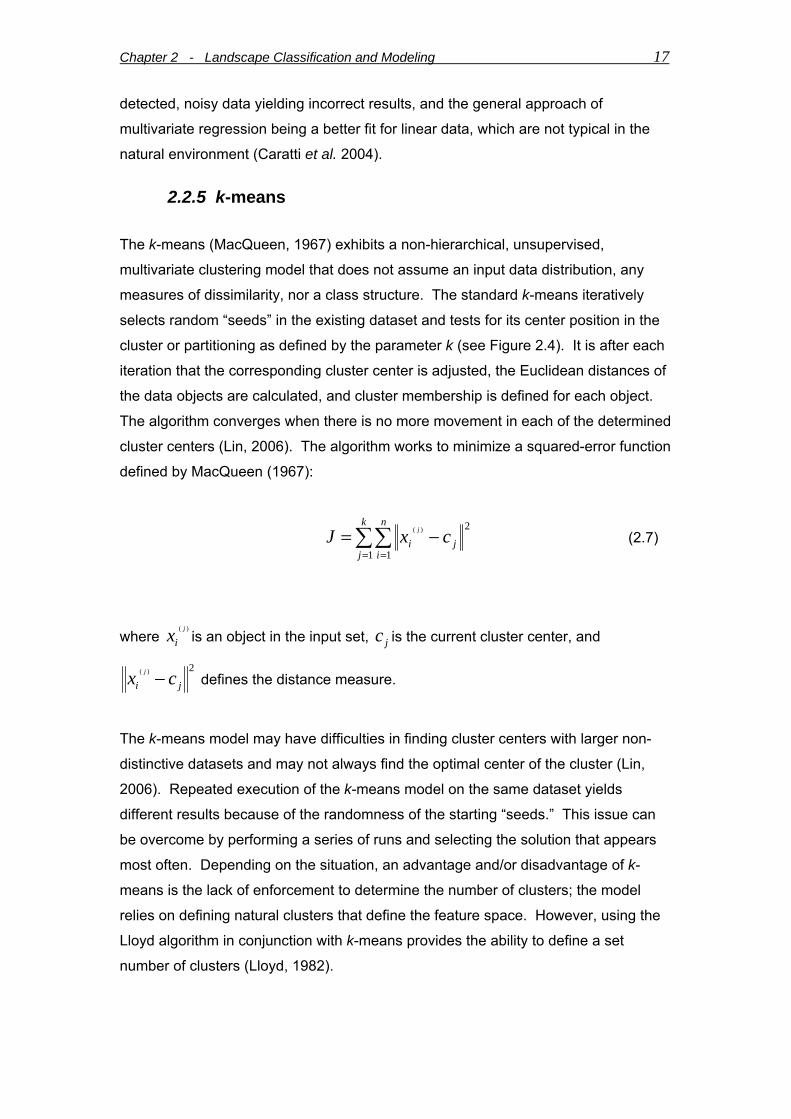
2.2.5 k-means

The k-means (MacQueen, 1967) exhibits a non-hierarchical, unsupervised,

multivariate clustering model that does not assume an input data distribution, any

measures of dissimilarity, nor a class structure. The standard k-means iteratively

selects random “seeds” in the existing dataset and tests for its center position in the

cluster or partitioning as defined by the parameter k (see Figure 2.4). It is after each

iteration that the corresponding cluster center is adjusted, the Euclidean distances of

the data objects are calculated, and cluster membership is defined for each object.

The algorithm converges when there is no more movement in each of the determined

cluster centers (Lin, 2006). The algorithm works to minimize a squared-error function

defined by MacQueen (1967):

∑∑= =

−=k

j

n

iji cxJ j

1 1

2)( (2.7)

where is an object in the input set, is the current cluster center, and )( j

ix jc2

jc−)(

ix j defines the distance measure.

The k-means model may have difficulties in finding cluster centers with larger non-

distinctive datasets and may not always find the optimal center of the cluster (Lin,

2006). Repeated execution of the k-means model on the same dataset yields

different results because of the randomness of the starting “seeds.” This issue can

be overcome by performing a series of runs and selecting the solution that appears

most often. Depending on the situation, an advantage and/or disadvantage of k-

means is the lack of enforcement to determine the number of clusters; the model

relies on defining natural clusters that define the feature space. However, using the

Lloyd algorithm in conjunction with k-means provides the ability to define a set

number of clusters (Lloyd, 1982).


Figure 2.4. A sample of 8000 points in the initial phase of k-means processing with random starting “seeds” placed in the input data space (a) and the final convergence stage (b). The cluster center, ,

is indicated by the large colored dot and parameter k=5 resulting in five distinctive cluster areas (Pelleg, 2004).

jc

Other variants of the k-means model that are used in multi-dimensional classification

include ISOCluster and fuzzy k-means. The ISOCluster model (Richards, 1986), or

Iterative Self-Organizing Clustering, uses the central idea of k-means, updating

cluster centroids until minimal distances are reached (i.e., convergence), with the

well-known ISODATA model (Ball and Hall, 1965) and the MLC (see Figure 2.5).

ISOCluster requires the number of clusters to be defined; however, if a more free-

form, natural clustering approach is needed, it is possible to set a high cluster

number (i.e., the parameter k) and then “aggregate clusters after interpretation”

(Eastman, 2006).


Figure 2.5. The ISOCluster model incorporates k-means, ISODATA, and the Maximum Likelihood Classifier, to organize and classify multivariate data.

ISOCluster is an unsupervised multivariate model that is commonly found in the

literature and is readily available in most image-processing and GIS software. As is

the assumption with the MLC, ISOCluster also assumes that the input data follow a

normal distribution. In some cases, data can be transformed into a normal

distribution by running a log-transformation (Ziadat, 2005).

Fuzzy k-means (DeGruijter and McBratney, 1988) is very similar to the standard k-

means model; the major difference is the application of the fuzzy-set theory allowing

a degree of membership in multiple cluster sets. This model has been used in

various research and appears to be gaining momentum in its application (Bolliger,

2005; Burrough et al., 2001; McBratney and DeGruijter, 1992; Minasny and

McBratney, 2002; Schmidt and Hewitt, 2004). Fuzzy k-means uses a similar iterative

minimization of the sum of square errors as standard k-means, but uses a term for

fuzzy membership, or the idea that a data object can belong, with varying degrees, to


more than one defined class. The model is defined by Minasny and McBratney

(2002), as follows:

(2.8)

∑∑= =

=n

i

c

kkiik cxdmJ

1 1

2 ),(φ

where n is the number of input data, c indicates the number of classes (equivalent to

k in k-means), the exponent φ is the fuzzy membership parameter that can range

from 1 - ∞, is the individual input data, is the centroid of k=n, and finally,

is the squared Euclidean distance between the data object and the class

centroid. The fuzzy membership parameter,

ix kc

),(2ki cxd

φ , produces a hard and discrete cluster

boundary at a minimum value of 1 and increases the degree of fuzziness as the

parameter approaches infinity, and it ultimately leads to the data object set to being

assigned to a single class.

In general, fuzzy-set based models for landscape classification offer an improvement

in terms of understanding the non-discrete boundaries that exist in natural processes.

However, difficulty arises in determining ideal fuzzy parameter values that 1) don’t

over-simplify the landscape with large fuzzy classes resulting in minimal class

distinction, and 2) provide enough realism and balance such that class membership

is not forced by strict boundaries or defined purely by the data objects. Bolliger and

Mladenoff (2005) provide a recommend that φ to range from 1.2 – 1.5 for landscape

classifications. An advantage to using a fuzzy k-means approach is gaining an

assessment of the uncertainty found in the data classes (Burrough et al., 2001;

Schmidt and Hewitt, 2004).

2.2.6 Ward’s Hierarchical Clustering

A statistical model commonly used in landscape classification is Ward’s (1963)

agglomerative hierarchical clustering (Bolliger, 2005; Bolliger and Mladenoff, 2005;

Lin, 2006; Osinski, 2003; Wardrop et al., 2005). The model groups the input data in

an iterative bottom-up (i.e., agglomerative) style, where in the first processing step all

data points, j , make up their own individual clusters, i , such that j = i . In a

hierarchical form, two data points that are most similar are grouped and the process

is iterated until there is only a single cluster remaining. Ward’s clustering differs from


other clustering models in that it does not use a distance metric such as Euclidean or

city-block, but rather a measure of minimum variance. All data, j , are evaluated for

their error sum of squares, which is a measure of information loss, and is defined by

, (2.9) 2

_

|| kixXESS ijkkji

⋅−= ∑∑∑

where represents the value for variable ijkX k in data j within a given cluster,

(Wiesner, 2008). A pair of data with the minimal error sum of squares creates the

first clusters in the hierarchy. The evaluation of the minimal error sum of squares is

repeated in the second processing step, but instead of evaluating individual data

point clusters, the cluster means that contain a larger data membership are used until

the final cluster is formed containing all data points. The result is something

resembling a tree, formerly known as a dendogram (see

i

Figure 2.6).

While agglomerative hierarchical clustering (i.e., Ward’s clustering) is a popular

choice for many applications, including landscape classification, it has clear

limitations. First, it is not possible to determine the number of natural clusters in the

data; instead, these must be defined with a priori knowledge, if available.

Additionally, Mangiameli et al. (1996) state that “to obtain the best cluster results, the

investigator must have considerable knowledge about the empirical data including

the number of natural clusters, the statistical distribution of observations within the

natural clusters, the presence of outliers, and the density of observations among the

natural clusters. The information required for an intelligent choice of cluster heuristic

is usually not available.” Lin and Chen (2006) also address biasing: “Ward’s method

tends to join clusters that contain a small number of sites, and it is strongly biased

when the clusters have roughly the same number of sites.” Ward’s clustering,

however, is well suited to handle large multivariate datasets and stands out among

other hierarchical clustering models because it uses a minimum variance rather than

a distance metric.


Figure 2.6. An example of the agglomerative hierarchical clustering for dominance of tree species in Wisconsin, USA (Bolliger et al., 2004).

2.2.7 Artificial Neural Networks

Artificial Neural Networks have been used in landscape classification analyses

(Bacao et al., 2005a; Bryan, 2006; Ehsani, 2007; Hilbert and Ostendorf, 2001; Hsieh

and Jourdan, 2006; Joy and Death, 2004; Lenz and Peters, 2006; Park et al., 2001),

but they are not as commonly used as the other models previously discussed.

Potential reasons for this may be the complexity of the process, the number of

parameters that need to be tuned, the many different types of ANNs, and the mixed

results that have been published (i.e., about ANNS being found to be useful or not

useful). ANNs show their strength and agility in handling complex, nonlinear,

distribution-free, high-dimensional datasets. The great variety of ANNs developed to

date includes the popular Multi-Layer Perceptron (MLP) network, the Radial Basis

Function (RBF) network, the Recurrent Neural Network (RNN), and the Adaptive

Resonance Theory (ART) network. ANNs have been used in the remote-sensing

field for many years in a research mode (Atkinson and Tatnall, 1997; Civco, 1993;

Richards and Jia, 1999; Tso and Mather, 2001), and they are beginning to find a

place in commercial remote-sensing software (Eastman, 2006). Additionally, ANNs

are used in some GIS analyses, but the processing steps are loosely coupled. To


the author’s knowledge, the only coupled commercial or open-source GIS/ANN

implementations are 1) ArcSDM (Spatial Data Modeler) (Sawatzky et al., 2004),

which focuses on mineral exploration but can be used for other applications in which

a spatial prediction is required, and 2) the JDEVS (Java Discrete Events System)

(Filippi and Bisgambiglia, 2004), which provides an environmental modeling

framework that links GIS and ANNs. The study reported here focused on the use

and application of the unsupervised ANN, SOMs. Further detail on ANNs and

specifically, SOMs, is provided in the following chapters.

Chapter 3 - Artificial Neural Networks 24

3.0 Artificial Neural Networks Because the objectives of this research are focused mainly on the pattern recognition

capabilities of ANNs, it is necessary to 1) understand their varying capability and

benefit for pattern recognition, and 2) understand the benefits and limitations of their

use in classifying the landscape. This chapter provides a basic understanding of

pattern recognition, soft computing, ANN models used in classification, and a more

detailed description of SOMs, which are the core ANN model used in this research.

A hierarchical approach is used to explain and define how SOMs fit into the bigger

realm of soft computing and how patterns can be used to classify data. Under the

broad umbrella of soft computing, ANNs offer a large array of resources to apply to

an even larger number of possible application areas. In general, ANNs capable of

solving classification problems can be categorized into “supervised” and

“unsupervised” ANNs. SOMs offer a well-recognized ability to handle unsupervised

classifications on large complex datasets. The concepts, procedures, algorithm, and

some of the mathematics of the SOM are presented. Finally, a simple demonstration

of the SOM using a red-green-blue (RGB) colorset illustrates how a complex and

randomized dataset can be organized and reduced in its dimensionality. While the

colors used in the demonstration make it easy to see and understand the strength of

the classification, the use of and potential for a SOM to reduce and classify nonlinear

multivariate data from the landscape must also be considered.

3.1 Pattern Recognition

As discussed by Bishop (1996), “pattern recognition encompasses a wide range of

information processing problems of great and practical significance.” Chapter 2.0 of

this report introduced some of the basic concepts of landscape classification and

further concepts will be considered here to emphasize the importance of pattern

recognition and the role it plays in ANN processing.

Brain functions can, seemingly with relatively little effort, distinguish objects in the

surrounding environment. The characteristics of the objects include color, shape,

texture, smell, etc., all of which help us to distinguish and capture, at varying levels of

detail, their function and state. The task of performing pattern recognitions in a

computational setting is one that has represented a scientific challenge for decades

and has become the focus of Artificial Intelligence. To grasp the simple pattern


recognition capabilities of the brain, consider the pattern examples shown in Figure

3.1 through Figure 3.3 (SFCC, 2007).

Figure 3.1. This illustration exemplifies an anomaly (far right) in a regular pattern space. The mind immediately picks up on the abnormality, which thus becomes a point of interest (SFCC, 2007).

Figure 3.2. This set of objects relates the brains’ natural ability to recognize patterns and fill in missing information. Note the only objects that actually exist in this illustration are four incomplete circles with varying amounts of missing information. Through pattern-recognition, four complete circles and a square are comprehensible (SFCC, 2007).

Figure 3.3. This illustration exemplifies the concept of proximity where the pattern on the left is viewed as a series of separate objects, the one in the middle is viewed as a single object (although it consists of separate objects), and the one on the right is viewed holistically as a single complex object composed of similar objects with different orientations (SFCC, 2007).

The examples illustrated can be related back to actual multivariate patterns and to

the challenges related to incorporating pattern recognition in a machine-learning

context. In the case of processing imagery for pattern recognition, the data are

processed as a multi-dimensional matrix. Interestingly, the three sets of patterns


shown in Figure 3.1 through Figure 3.3 are rooted in the early 20th century work by a

group of German psychologists who identified the ability of the human brain to

pattern in various modes, and established “mental laws” referred to as the Gestalt

Principles. Consider for a moment, the capability of the human brain to process a

single day’s worth of information and logistics as well as its adaptive nature for

survival. The brain has the ability to “process millions of visual, acoustic, olfactory,

tactile, and motor data, and it shows astonishing ability to learn from experience,

generalize from learned rules, recognize patterns, and make decisions.” (Kecman,

2001). The science of Artificial Intelligence (AI) works to mimic the brain’s massive

capability.

3.2 Soft Computing

Artificial Neural Networks are part of a larger field of study under the overarching

topic of “soft computing.” Support Vector Machines, evolutionary and genetic

algorithms, swarm intelligence, and fuzzy logic models also can be included in soft

computing. These computational models were largely developed to deal with the

complexities and unknown boundaries of large multivariate datasets. Kecman (2001)

refers to soft computing methods as “universal approximators of any multivariate

function…of particular interest for modeling highly nonlinear, unknown, or partially

known complex systems, plants, or processes.” The complexities observed in the

landscape exhibit characteristics for which soft computing is well suited. The notion

of soft computing is contrary to “hard computing” methods where strict logic is used

to achieve a definitive and precise answer. The paradigm of soft computing

addresses several characteristics of uncertainty in the landscape, including 1)

observations and data representations; 2) understanding of physical and biological

processes; and 3) our model representations of landscape processes. The

acknowledgement of these uncertainties, in addition to the fuzzy nature of the

landscape provides an argument for using soft computing methods to better

understand and represent the landscape. The following sections focus on ANNs to

further the conceptual understanding of these computational models for application to

landscapes.

3.3 Fundamental Basis of Artificial Neural Networks

The initial concept of ANNs as dealt with by McCulloch and Pitts (1943), who

formalized the concept of an artificial neuron. Work on ANNs was relatively non-


existent until the early 1980s, when Hopfield (1982) set the stage for using ANNs in a

wide array of multi-disciplinary fields.

A formal definition of an ANN model is provided by Aleksander and Morton (1990):

“A neural network is a massively parallel distributed processor that has a natural propensity for storing experimental knowledge and making it available for use. It resembles the brain in two respects: 1) Knowledge is acquired by the network through a learning process. 2) Interneuron connection strengths known as synaptic weights are used to

store the knowledge.”

ANN models work to mimic the functions of neuron cells in the brain. A basic

representation of the neuron and its interaction with other neurons is presented in

Figure 3.4. Communication of information among the brain’s neurons is conducted

through electrical pulses of various frequencies and magnitudes. These electrical

pulses are produced as a response to the input of information into and within the

body and allow communication not only within the brain but with all body functions

(i.e., muscle response, organ function, etc.). The primary components of the neuron

are the nucleus, dendrite, axon, and synapse. In general, dendrites are responsible

for receiving information from other neurons, the axon sends an electrical signal (i.e.,

information) to neighboring cells, and the synapse is the connection point between an

axon on one cell and a dendrite from a neighboring cell.

Figure 3.4. A simplified graphic representation of a neuron cell processing and transmitting information from cell to cell (adapted from Lingireddy and Brion, 2005).


Neurons function in a massively parallel manner as signal communications occur

across many cells, and each cell can have as many as 10,000 dendrites that are

continually being fed electrical signals (Smith, 1996). The many sources of signals

being fed into an individual cell are resolved into a single signal, which is output

through the axon and delivered to associated dendrite receptors. A schematic

representation of the neuron cell communication via an ANN is presented in Figure

3.5. ANN models retain some of the neurological vocabulary to describe the

components of the system. As represented in Figure 3.5, the spheres are “neurons”

and the lines connecting the neurons are “synapses.” In real neuron cells, the

synapses inflate and contract to control the sequence of the signals in terms of their

magnitude and frequency. The synapses in an ANN model function similarly where

“connection weights” along the individual synapses are adjusted and optionally,

imposed delays are applied to assist in the learning process. The hidden layer

shown in Figure 3.5 provides an “activation function,” which transforms the sum of

the input data into a data signal using one of many possible functions, including

logistic (sigmoid), hyperbolic, exponential, sine, and square root. Table 3.1 is a

comprehensive list of activation functions. Increasing the number of hidden layers

allows the neural network to handle even more complex problems; however, caution

must be exercised so as to not over-commit the input data, thereby causing

generalizations (Lingireddy and Brion, 2005; Rohwer et al., 1994).

Figure 3.5. A common and simple ANN schematic that represents the flow of information from the input data, to the receipt of the input neurons, to weighting and evaluating of data, to signal adjustments in the hidden layer, and finally the resulting output data (adapted from Principe et al., 2000).


In a supervised ANN classification, the input data are compared to a set of training

data that defines “truth” in the data relationships. The error of the solution is obtained

with each iteration, and the connection weights are adjusted (increased or

decreased) according to how the output data compare with the training data. The

ultimate goal is to determine the combination of connection weights that provide the

minimum error between output and training data. The weighting process is used as a

probability measure where weights are increased to represent higher probabilities

and are decreased for weaker probabilities. Therefore, as input data signals are

presented to the ANN, the strongest probability and most frequent occurrence of the

signal can be grouped with others. This process is repeated until the optimal solution

with the various combinations of connection weights is determined. The optimal

solution, often referred to as a “trained ANN” or “trained net,” can then be used to

classify future input data where the class isn’t known. A common approach used to

assess a trained net is to use two-thirds of the existing training data for establishing

the neural network, then run the remaining one-third of the training data through the

model to evaluate how capable the model is at making the predictions.


Table 3.1. Common activation functions used in ANN models (StatSoft, 2003).

Function Name Function )(xf Data Range

Identity x +∞∞− ,

Logistic

(Sigmoid) 111

−− e

)1,0( +

Hyperbolic

xx

xx

eeee

−

−

+−

)1,1( +−

Exponential xe− ),0( +∞

Softmax

∑i

i

x

xe

)1,0( +

Unit Sum

∑i

ixx

)1,0( +

Square Root x ),0( +∞

Sine )sin(x )1,1( +−

Ramp

⎪⎭

⎪⎬

⎫

⎪⎩

⎪⎨

⎧

≥++<<−

−≤−

0111

11

xxx

x )1,0( +

ANNs are considered semi-parametric classifiers because they use both parametric

discriminate functions and nonparametric shape discriminators. The combination

provides a unique and dynamic approach to traditional statistical classifiers (Principe

et al., 2000). A common use of ANN models seeks to solve regression, classification

or pattern recognition, prediction, and signal processing problems, all of which

routinely are used as components of decision support systems. While ANNs have

their foundations in conventional statistical models, they differ in that 1) Gaussian, or

normal, distributions of data are not required; 2) linear or nonlinear data are

acceptable for inputs; 3) adaptive learning is an integral part of the model; and 4)

there is a high degree of error tolerance that can throw off results in common

statistical methods, provided a reasonable signal-to-noise ratio exists in the data.

ANN models make no assumptions about the input data, other than they expect

numbers, not alphanumeric characters, and will adjust the weights of the internal


network directly from the input data. As stated by Perus and Krajinc (1996), “the

most important thing is that ANNs allow a different view of problems which cannot be

solved by [exact] statistical methods due to their theoretical limitations.” In addition,

natural data cannot always be described with low-order statistical parameters,

because these elements and relationships between elements can exhibit nonlinear

associations. For this reason, the adaptive characteristics of ANNs are more

effective and allows for an automatic determination of parameters through an

evaluation and repeated weighting adjustment of the input data space (Kohonen,

2001). In the most commonly used ANNs, the use of “feedback loops” provides an

adaptive capability and enables ANNs to evaluate their own performance, which is

often a measure of mean square error of model prediction value and the targeted or

trained value (see Figure 3.6). The performance values are used to continually

adjust the parameters of the ANN to match some known condition, allowing for

learning and training to improve upon the output results. The idea of performing

continual adjustments introduces the notion of “adaptive learning” and is especially

effective for data that continually evolve in time and space, such as meteorology,

vehicle traffic, disease spread, and landscape processes.

Figure 3.6. Result of a simple multi-layer perceptron ANN evaluating the MSE over model iterations. Once a sufficient MSE is reached, the optimal solution is obtained, meaning ANN output values closely match the training values and an underlying relationship has been established between input data vectors and resulting output.

The adaptive learning concept found in ANNs provides a significant advantage over

traditional statistical techniques; however, ANNs do have some known

disadvantages. First, it is possible to present too much training data to an ANN (too

much of a good thing), in which case the model is “over-trained” and crosses a

threshold that causes a degradation in model performance by increasing mean

square errors. Next, ANNs can have some difficulty in classifying a given data


pattern where no appropriate class exists. In such cases, the “out-of-class” data are

lumped with the category of data that is closest or most similar. While ANNs have

proven themselves in a wide array of applications, including hydrologic forecasting, a

common criticism is that they are often used as a “black box model,” for which input

is presented and output is generated, and no understanding of the internal

mechanics are required. As is commonly the case with hydrologic modeling, for

instance, a physically based model is constructed to transport and explain the

movement of water through each component of the hydrologic cycle. The

governance of strict mathematical bounds is used to mimic the process of water

transport through its various routes (e.g., overland flow, groundwater,

evapotranspiration, precipitation, etc.). With an ANN, the detailed physically based

processes are effectively lumped into the “black box” and the determined driving

input parameters to water transport (e.g., precipitation, temperature, relative

humidity, soil moisture, vegetation, and soil type, etc.) are presented along with

known outputs (e.g., stream outflow), and thus the ANN determines the data

relationships between the input and output without needing knowledge of the flow

transport physics.

3.4 Common Types of Artificial Neural Networks

Numerous types of network structures are found in ANNs, each possessing a unique

behavior and purpose. In some cases, multiple network structures are used together

to take advantage of their respective strengths. The topology of the ANN dictates the

type of network and the number and shape of the activation functions. This section

briefly discusses supervised and unsupervised ANNs used for classification, that are

distinguished by the use or no use of training data, respectively.

3.4.1 Supervised Artificial Neural Networks

Most ANNs fall under the supervised category. A supervised ANN, by definition,

uses a training dataset for which both the input data and resulting output data are

known. The supervision process defines relationships between input and output data

by iteratively adjusting connection weights and reducing model errors. This

adjustment occurs both at the individual neuron scale and globally through the

model, attempting to reduce the model error over time.


A classical example to explain the ANN training process is Fisher’s iris dataset

(Fisher, 1936). This dataset captures multivariate information for three known

species of the iris flower: 1) setosa, 2) virginica, and 3) versicolor. The measured

variables of the iris flowers, as shown in Table 3.2, include 1) petal width, 2) petal

length, 3) sepal width, and 4) sepal length. For each species, 50 samples were

measured. While Fisher used this dataset to develop a linear discriminant model that

helped to identify the flower species based on the physical measurements, it also is a

good representation and sample dataset to use to explain what is required for a

training dataset in a supervised ANN model. Additional and more comprehensive

datasets can be found on the website of the University of California’s Irvine Machine-

Learning Repository: http://archive.ics.uci.edu/ml/.

Table 3.2. A small sample of Fisher's multivariate Iris flower dataset (Fisher, 1936).

Sepal Length Sepal Width Petal Length Petal Width Species 5.1 3.5 1.4 0.2 setosa 4.9 3.0 1.4 0.2 setosa 7.0 3.2 4.7 1.4 versicolor 6.4 3.2 4.5 1.5 versicolor 6.3 3.3 6.0 2.5 virginica 5.8 2.7 5.1 1.9 virginica

The requirements for a supervised neural network can be substantial in terms of

generating a large enough training dataset to capture the variability of the input data.

The ANN learns to recognize the variable conditions and adapts itself to respond

appropriately. It is ideal to have a large enough cross section of input data to capture

the data variability so, while the ANN model is training, it can establish an effective

solution of network weights and allow intelligent output if the system encounters data

conditions not previously known. Establishing a supervised ANN model

throughought the training phase can be time consuming and require tuning of

parameters in the model. Parameters such as learning rate, step size, weight decay,

momentum rate, synapse delays, beta/gamma conscience, memory, and more are

used to assist in the model learning.

3.4.1.1 Multi-Layer Perceptron The most commonly used supervised ANN model is the feed-forward Multi-Layer

Perceptron (MLP). The MLP is linked with the back-propagation learning algorithm,

which allows for the iterative adjustment of weights to correct errors in the model

(Rumelhart et al., 1986). This neural network is general in nature, allowing for its use

in a wide variety of applications including pattern recognition (Ermini et al., 2005;


Freeman and Skapura, 1991). The feed-forward component of the MLP states that

the output vectors produced by the ANN are a function of the input vectors and some

weighting process; this is an important distinction to make because variability exists

between networks (e.g., Recurrent Neural Networks). MLPs are best suited for

pattern recognition and/or classification type problems.

The basic structure of the MLP, shown in Figure 3.5, includes the input layer, one or

more hidden layers, and an output layer. The input layer is fed with vectors of data,

also termed “codebook vectors,” and, in the training phase, a related output value for

each codebook vector is offered. The hidden layer is variable in the number of

neurons available; thus, depending on the complexity of the problem, more neurons

may provide a better solution. However, excessive placement of neurons in the

hidden layer can also over-fit the model, thereby creating degraded results.

The MLP exhibits three important characteristics. First, the network is massively

parallel and massively interconnected where each neuron in each layer connects to

every other neuron in the next layer. Second, the neurons process data in a

nonlinear state and pass codebook vectors through a hyperbolic or logistic (sigmoid)

type of activation function (see Table 3.1). Third, the final classification of data is

resolved by dividing the pattern space using hyperplanes (StatSoft, 2003). As stated

by Ermini et al. (2005) the role of the MLP “is not to fit the observed data but to model

a process by generalizing the learned experience to other cases not represented in

the training database.”

3.4.1.2 Radial Basis Function Neural Networks Radial Basis Function (RBF) neural networks are based on nonlinear regression and

classification networks, which differ from the MLP network on several fronts. The

classification in the pattern space is defined by spheres, such that data is classified

by the radius of each data point from the center of the data distribution. These

networks exhibit a single hidden layer and are typically composed of a very large

number of neurons. These neurons apply a nonlinear Gaussian surface activation

function that is then fed to output linear weights (Govindaraju and Zhang, 2000). The

overall design of the RBF network is simpler than the MLP network, leaving less to

experiment with in terms of determining the numbers of hidden layers and total

neurons within each hidden layer. In addition, the training of the RBF network is

reported to be much faster than the MLP and can handle noisy input data very well.


However, the network also has limitations in that it typically doesn’t behave well in

data space that hasn’t been included in the training data (Govindaraju and Zhang,

2000). The RBF network has been successfully used for hydrological applications on

landscapes (Govindaraju and Zhang, 2000; Lin and Chen, 2005; Moradkhani et al.,

2004).

3.4.1.3 Probabilistic Neural Networks The Probabilistic Neural Network (PNN) is a supervised ANN model that has its roots

in Bayes classifiers and is a subset in a group of neural networks called radial basis

networks. PNN relies on the RBF and probability distribution function (pdf) to classify

data (Nikolaev, 2008). Through the training process, the PNN learns to approximate

the pdf of the training sets, which ultimately assigns a degree of membership to the

defined classes. The PNN is structured using four layers consisting of the input,

radial basis layer, competitive layer, and output (Demuth and Beale, 2007; Ermini et

al., 2005). The basic process brings the input data in, computes the distance

between the input and trained data vectors based on the RBF, sums the vectors, and

presents a vector of probabilities to the competitive transfer function where the vector

with the maximum probability is chosen as the winner (Demuth and Beale, 2007).

While PNNs aren’t as commonly used as other supervised ANNs, the literature

suggests their use in classifying the landscape has fair and promising results.

Figueiredo and Gloster (1998) state that the PNN classifier “presented good

accuracy, very small training time, robustness to weight changes, and negligible

retraining time.” A landslide hazard assessment conducted by Ermini et al. (2005)

evaluated PNN models and found only results to be a fair predictor when compared

to field data. Finally, in the ArcSDM application (Sawatzky, 2004), PNN is integrated

as a part of the standard tool set for predicting mineral occurrence. One reported

disadvantage of PNN is the large memory and computational power required to run it

(Demuth and Beale, 2007).

3.4.2 Unsupervised Artificial Neural Networks

Unsupervised ANNs offer a large research area and show considerable promise for

use in many fields. Their use is not widespread like that of supervised ANNs, yet

unsupervised ANNs seem to have a future potential for providing a more


autonomous capability in decision-making processes. Unsupervised ANNs have the

ability to discover structure and natural clusters within a set of data for which no

classes have been defined. Unsupervised neural networks can be beneficial in at

least three basic conditions. First, in a supervised ANN, it is possible to force input

data into defined classes, while an unsupervised ANN might reveal a distinction in

the natural data. Second, there are situations for which no class information is

available because a given situation has never occurred, has only occurred in limited

space, or the data are entirely unknown. Finally, unsupervised ANNs are capable of

discovering and clustering complex data relationships that can lead to determining

class definitions or revealing previously unknown data relationships that weren’t

readily obvious.

The unsupervised ANN works to extract knowledge by exploring redundancy in the

dataset, thus finding and grouping similar data patterns. This type of processing is

especially effective for dealing with complex multivariate data where it may be difficult

to determine data relationships and patterns. Unsupervised neural networks rely on

varying network topologies and adjustment parameters such as initial neighborhoods,

decay functions, and step size to control the internal learning. The most commonly

used unsupervised ANN is the SOM, also referred to as a Kohonen Network,

Kohonen Map, or Self-Organizing Feature Map (SOFM). The premise of this

research is based upon the understanding, integration, and use of the SOM in GISc.

The following section provides additional detail on SOM neural networks.

3.4.2.1 Self-Organizing Maps The SOM is an unsupervised ANN that projects and maps high-dimensional,

complex, nonlinear data to iteratively organized clusters, in a topology-preserving

manner, for the creation of a low-dimensional discrete data space. The space can be

used for a wide variety of purposes including speech recognition, industrial process

control, image analysis, data mining, DNA sequencing, data visualization, and more

(Bryan, 2006; Chon et al., 1996; Kohonen, 1982; Kohonen, 2001; Schmuker et al.,

2007). In broad terms, the SOM model takes input data, establishes the nonlinear

statistical relationships in a high-dimensional dataset, and transforms the data into a

topology-preserving geometric structure in low-dimensional form. The SOM “…can

be characterized as a two-dimensional, finite-element ‘elastic surface’ or network that

is fitted to the distribution of the input samples” (Kohonen, 2001). The added value of

the SOM is its ability to discover hidden data patterns, structures, and relationships in


multivariate datasets. It also can conceptualize and map data in one-dimensional (1-

D), two-dimensional (2-D), or three-dimensional (3-D) output space using a variety of

topological structures (e.g., linear, rectangular, toroidal, spherical, cubic, etc.).

The concepts of the SOM were originally proposed by Willshaw and von der

Malsburg (1976), but it was Kohonen (1982) who developed the algorithms and has

actively fostered their growth and capability. Because the SOM classifies data in an

unsupervised form, no training data are presented to the network; thus, there is no a

priori knowledge about the data distributions or the placement of data into discrete

output space. In addition, no hidden layers are established in this type of network;

instead, the input data and neurons are applied to a single combined input-hidden

layer of weighted connections (see Figure 3.7). As mentioned previously, the SOM

network establishes the topologic structure of the data. This structure is obtained by

repeatedly presenting the input data signals to the network and adjusting the network

weights to create “meaningful order, as if some feature coordinate system were

defined over the network” (Kohonen, 2001). With SOMs, there are no assumptions

about the number of classes that need to be created; in fact, some researchers

suggest the use of a neuron for every attribute in the input space just to ensure a full

representation of the data (Bryan, 2006; Chen, 1995). Using a high number of

neurons (i.e., classes) can provide a meaningful way to initially understand

relationships and patterns in the data. This approach can be followed by

experimentation with a specific number of classes to identify a balance between the

number of classes and proper data representation. It should be made clear that in

SOMs each neuron introduced into the network attempts to establish and compete

for its ownership over sets of similar data. However, this practice does not mean that

every neuron has to be used. The SOM only uses the number of neurons necessary

to represent the data.


Figure 3.7. A representation of the single-layer Self-Organizing Map process as it presents data to the network, competes, and maps organized data clusters to a defined 1-D, 2-D, or 3-D topology.

An Overview of the SOM Algorithm Self-Organizing Maps fall under the heading of “competitive soft-learning algorithms,”

which means that the neurons in the network compete against each other to match

input data that are randomly presented to the neurons. The algorithm defined herein

is summarized from the works of Kohonen (2001), Fritzke and Loos (1997), and

Schmuker et al. (2007). When the SOM network is first initialized, a random set of

network weights ( ) is generated (see ijw Figure 3.8), after which the competition and

learning process begins with the random presentation of the input data signal or

codebook vector, (ξ ) from matrix ( ), which takes the following structure: X

(3.1) ⎪⎪⎪

⎭

⎪⎪⎪

⎬

⎫

⎪⎪⎪

⎩

⎪⎪⎪

⎨

⎧

=

nninnn

ni

ni

xxxx

xxxxxxxx

X

,,2,1,

,2,22,21,2

,1,12,11,1

,...,...,......

,...,...,,...,...,


The “winning” neuron, ( ξwn ) is then determined by evaluating the random codebook

vector that was presented to the network, (i.e., a single entry of multivariate data from

input data matrix) against all network neurons in the model. A graph-based distance

measure such as the L1-norm (i.e., the Manhattan distance or the city-block metric) or

Euclidean distance is calculated to determine the absolute minimum value between

the input vector (ξ ) and the training neuron vector (η ), after which the “winning”

neuron is identified and defined by ),( ξηd .

Figure 3.8. A representation of the random weight initialization that occurs in the first phase of the SOM learning process. Input codebook vectors are presented to the randomly weighted neurons and the organization and learning process begins.

Once the “winning” neuron is selected, similar neighboring neurons are pulled toward

the winner to update the overall topology and network weights, thus furthering the

organizational process. This process is repeated for the set number of time-steps or

until an overall measure of network structure and global minimum error is obtained.

At each time-step, the training neurons are updated by the following term:

η )(),,()(λ ν η ξ η−⋅⋅=Δ tnt w (3.2)

where ( t ) is time, (λ ) is a learning rate with indices ( i ) and ( f ), which state the

initial time-step and maximum time-step, respectively, and are defined by


.)(

maxtt

i

fit ⎟⎟

⎠

⎞⎜⎜⎝

⎛=

λλ

λλ (3.3)

In a standard SOM, there is a time-decaying kernel neighborhood function (ν ),

where the neurons surrounded by the winner learn together, thus causing a pulling

and stretching effect on the winning neuron and its neighbors. A Gaussian function

is often used for the kernel neighborhood (see Figure 3.9) and is expressed as

⎟⎟⎠

⎞⎜⎜⎝

⎛−= 2

2

)(2),(

exp),,(t

nndtn wtopo

w σην

, with (3.4)

.)(

maxtt

i

fit ⎟⎟

⎠

⎞⎜⎜⎝

⎛=

σσ

σσ (3.5)

where ( ) defines the shortest path in graph space. topod

Figure 3.9. A Gaussian function is often applied to a time-decaying kernel neighborhood to update the “winning” neuron and those in the effective area. This process makes the SOM learning efficient and stable. The kernel is defined by the center point and the kernel neighborhood is represented by the red rings, which become smaller with each time-step.


In the early learning stages, the kernel neighborhood is large. As the learning

progresses, the effective neighborhood becomes smaller, more refined, and less

influential—eventually maintaining a minimum neighborhood distance as the

competitive learning process continues. The projection of the SOM network over the

data is directly influenced by the time-decaying kernel neighborhood where the major

establishment of the network occurs early in the process. Snapshots of the SOM

projection over time are presented in Figure 3.10, where T=0 are the randomly

initialized neuron locations and T=5000 is the final result. Note that in T=1000, the

neurons appear to be heavily grouped in one area and in general appear to be

swarming in a specific direction. This is a specific example of the effect of a time-

decaying kernel neighborhood where many neurons, rather than just one, are

learning at the same time-step. In the case where a minimum neighborhood distance

of 0 is specified, only the winning neuron is impacted. However, a minimum

neighborhood of 0.05 – 0.5 is common. The time-decaying kernel function has a

distinct benefit of making the model come to solution more efficiently while running in

a stable and safe manner (Kohonen, 2001).

The details of the SOM algorithm can be summarized as follows:

1. Initialize the weights of the training neurons (η ) to small random values.

2. Randomly select a codebook vector (ξ ) from data matrix ( X ) for

presentation to the network.

3. Calculate the distances (Euclidean or Manhattan) between the codebook

vector (ξ ) and the weights ( ijw ) of all neurons.

4. Select the “winning” neuron ( ξwn ) from the set with the minimum distance

),( ξηd .

5. Update the weights of the winner (Eq. 3.2 and Eq. 3.3)

6. Update the weights of the neighbors according to the distance from the

“winning” neuron using a Gaussian function (Eq. 3.4)

7. Increase the time-step and repeat all steps in the algorithm until the maximum

time or minimum error tolerance is reached.


Figure 3.10. The SOM process captured at multiple iterations reveals the competition, learning, and projection of neurons over the input data space. Note that with an increase in iterations, the decaying kernel neighborhood function has less influence on the overall network structure and focuses on the learning and competition with individual neurons and their immediate neighbors.

Demonstration of a Self-Organizing Map This section presents a simple demonstration to help understand the SOM and its

applicability to organizing and reducing the dimensionality of complex data. The

demonstration takes a complex 3-D image dataset and reduces the dimensionality

while generating topological relationships. This type of demonstration is easier to

understand because we are clustering colors and the result can be understood

visually, thus, no further classification process is needed after the SOM training is

complete.

A complex image is generated using a small script to randomly produce three

values— red, green, blue (RGB)—each with a possible range of 0 – 255. The result

is an image of the size 450x300 pixels composed of 135,000 total values (Figure

3.11). The objective of using the SOM for this demonstration is to classify the


complex 3-D data (i.e., red, green, and blue) and reduce the dimensionality of the

original image to a size of 64x64 pixels, and then to 32x32 pixels. Within the

randomly generated pixel values for the original image, there is a total of 16,777,216

possible color values, which the SOM reduces and classifies to a possible 4,096

values (i.e., 64x64), then again to a possible 1,024 values (i.e., 32x32).

Figure 3.11. A randomly generated 450x300 RGB image with 135,000 values used as input to a SOM training process.

To begin, the 2-D SOM array is initialized with random weights (see Figure 3.8 and

Figure 3.12), after which the competitive learning process begins to structure and

project the data in a way that is similar to what is presented in Figure 3.10.

Figure 3.12. The random initialization of neuron weights in a 2-D grid is presented. Each pixel in the grid is representative of a single neuron.

The final grid structure of the SOM training is presented in Figure 3.13. For

comparison, a 32x32 2-D SOM also was trained with the same input data as the


64x64 SOM and these results are presented in Figure 3.14. Keep in mind that

because the SOMs are initialized with random weights at the beginning of each

training, the topological order and projection of the data vary in their location (i.e., the

clusters of red-like colors currently show up in the lower-middle portion of the 64x64

grid and on the next run, these may show up in the upper left-hand corner).

However, the underlying assignment and clustering of data remain nearly or exactly

the same.

Figure 3.13. The final result of the SOM training from a 450x300 dataset reduced and organized into a 64x64 grid.


Figure 3.14. A 32x32 2-D trained SOM using the randomly generated source data presented in Figure 3.11.

Chapter 4 - The Adaptive Landscape Classification Procedure 46

4.0 The Adaptive Landscape Classification Procedure This chapter explores a procedure (i.e., the ALCP) developed to harvest large

amounts of landscape-based data, both spatial and spatio-temporal, into discrete and

homogeneous classes by using the powerful capabilities of GIS and SOMs. A

discussion ensues on the purpose and background for developing the ALCP and

further discusses the specific components and operating mechanics including the

data types that can be used, currently supported data themes, the GIS/SOM software

linkage, and visualization and analysis of the classification results.

4.1 Purpose and Background

It is well recognized that landscapes evolve over time through a process called

“ecological succession” (Cowles, 1911; Gleason, 1927). This evolution is spawned

by an array of complex interrelations of spatially distributed variables, including

geology, soils, precipitation, temperature, solar radiation, terrain, fluvial processes,

crustal movement, mass-wasting events, chemical and physical weathering, fire

events, meteorological extreme events, climate change, and varying anthropogenic

influences. Because of this understanding of landscape evolution and its many

possible variables, it is necessary to consider adaptability in producing discrete and

homogeneous measures of the landscape and in providing a method that is adaptive

to a wide range of different landscape, process, and variable types. For example, the

ALCP can be used to gain an overall perspective of the landscape, incorporating all

variables that are defined to take a part in the landscape, or evaluate specific

phenomena in the landscape such as probable sites of mass-wasting, measures of

habitat quality, hydrologic response, groundwater recharge zones, snow

accumulation properties, etc. The newly introduced ALCP is designed to be generic

enough to mix the variables of interest, develop a pattern of these variables, and then

evaluate the patterns for similarity across the landscape. Figure 4.1 provides an

example of four single-variable data patterns found in 10 separate sub-watershed

catchment areas. These individual patterns are captured and combined to create a

single pattern of multiple variables that is then used for the similarity analysis. As

stated by Bathgate and Duram (2003), “Although the landscape is a continuum, it can

be classified into discrete categories….” The process of using multiple metrics on

the landscape can be likened to the idea of multi-spectral analysis in remote sensing

(Brown, 1998).


Figure 4.1. Four variables for 10 sub-basin areas are presented to illustrate different data patterns in the landscape.


A core component of the ALCP is based on using pattern-recognition technologies

developed in the machine learning and evolutionary computing sciences. The

computational algorithms available to perform pattern recognition have been

dramatically enhanced by rapid developments in evolutionary computing over the

past few decades. Evolutionary computing methods, such as ANNs, SVMs, genetic

algorithms, swarm intelligence, simulated annealing, and fuzzy logic, have made

voice recognition, character recognition, data mining and/or search engines, medical

diagnosis, stock market analysis, and computer gaming and/or simulators common

features in modern society, and perhaps even without our recognition of what is

driving these processes. These new capabilities significantly augment the statistical

pattern recognition algorithms that were the basis of earlier pattern recognition

methods. It should be noted that while the focus of the study reported here is on the broader

landscape scale, there is nothing about this procedure (as long as the required data

are available) that would limit the ability to conduct similarity analysis on a fine scale.

For example, a 500-m reach of river could be evaluated for its aquatic habitat, which

might include variables such as river bathymetry and terrain-based derivatives, water

flow, flow velocities, current directions, substrate, nutrient availability, riparian

vegetation, aquatic vegetation, woody debris, etc. Similarly, the procedure can be

used for broader-scale analysis on a regional, continental, or global basis.

4.2 The Components and Structure of the ALCP

The ALCP relies on a hybrid mixture of basic and advanced geospatial processing

and analysis; a spatially enabled database for data input, storage, and queries; a

statistical processor; a Self-Organizing Map (SOM) model to analyze and cluster

input signals; and an external wrapper module to tie the components together. An

overview of the components and procedural flow of the ALCP is provided in Figure

4.2. The following four major components of the ALCP are discussed in the ensuing

sections:

• Source Data Elements

• Geospatial Processing

• SOM Model and Post-Processor

• Visualization and Analysis.


Figure 4.2. An overview of the structure and flow of the ALCP.


4.3 Source Data Elements

Much of the ALCP revolves around the source data used to conduct the classification

process. Figure 4.2 shows most of the datasets collected and derived for use and

testing in the study. While these data cover most of what would typically be needed

for landscape-level analysis, the choice of data required for analysis fundamentally

depends on the problem being addressed. For example, a multivariate ecoregion

study by Hargrove and Luxmoore (1998) considered detailed soils data including the

nitrogen content, soil-water capacity, and organic content of the soil as well as other

climate-related variables. An early design of the ALCP established a need to

incorporate a range of data types, thereby providing adaptability in the data inputs.

As such, the data elements for this study can be categorized into four primary

categories: 1) continuous, 2) categorical, 3) discrete, and 4) spatio-temporal, all of

which are described in the ensuing sections. The data and methods implemented in

the ALCP for possible use in landscape classification are summarized in Table 4.1.

4.3.1 Continuous Data

According to Worboys and Duckham (2004) continuous “if small changes in location

lead to small changes in the corresponding attribute value…” for a dataset.

Continuous data are commonly found in the form of raster, or pixel-based, data such

as elevation, temperature, soil moisture, and imagery and/or remote-sensing data.

The data plotted in Figure 4.1 and Figure 4.3 are representative of continuous data of

elevation and elevation data derivatives that are characterized by a smooth and

continuous transition from one point to the next. This type of data is by far the most

commonly used in the ALCP, largely due to the strong basis of primary and

secondary terrain-based data and remote sensing derived datasets. The ALCP

evaluates each continuous dataset and derives descriptive statistical measures for

each “spatial container” (discussed in Section 4.4.1) for presentation to the SOM

model.


Figure 4.3. Two examples of continuous datasets that are raster-based and characterized by smooth transitions between the attributes.

Table 4.1. Terrain-based data processed and extracted within the ALCP.

Data Reference Method

Continuous Data

Pit-Filled DEM (Planchon and Darboux, 2001)

Slope Fit 2-Degree Polynomial

(Zevenbergen and Thorne, 1987)

Aspect Fit 2-Degree Polynomial


Curvature Fit 2-Degree Polynomial


Plan Curvature Fit 2-Degree Polynomial


Profile Curvature Fit 2-Degree Polynomial


Convergence Index (Koethe and Lehmeier, 1996)

Solar Radiation (Wilson and Gallant, 2000)

Flow Direction & Accumulation (Tarboton, 1997)

Flow Sinuosity (Olaya, 2004)

Overland Flow Distance to Channel (Conrad and Ringeler, 2007)

Vertical Distance to Channel (Conrad and Ringeler, 2007)

Topographic Wetness Index (Moore et al., 1991)

Stream Power Index (Moore et al., 1991)

Length-Slope Factor (Moore et al., 1991)

Topographic Roughness Index (Riley et al., 1999)

Soil Depth Multi-Layer Soil Characteristic Database


(Miller and White, 1998)

Soil pH Multi-Layer Soil Characteristic Database


Soil Water Capacity Multi-Layer Soil Characteristic Database


Soil K-factor (particle transport) Multi-Layer Soil Characteristic Database


Categorical Data

Landform Class (Peucker and Douglas, 1975)

Land Cover

Multi-Resolution National Land Cover

Database (NLCD) (Homer et al., 2004)

&

Global Land Cover Characterization Program

(GLCP) (Loveland and Belward, 1997)

Discrete Data

Contributing Area (Tarboton, 1997)

Channel Network (Tarboton, 1997)

Channel Gradient ALCP-Generated

Channel Aspect ALCP-Generated

Catchment Area ALCP-Generated

Catchment Perimeter ALCP-Generated

Catchment Elongation Ratio ALCP-Generated

Channel Density ALCP-Generated

Longest Channel Length ALCP-Generated

Mean Catchment Slope / Aspect ALCP-Generated

Spatio-Temporal

Soil Moisture Remotely-Sensed Microwave Radiometer

(Njoku, 2007)

Normalized Difference Vegetation Index Normalized Difference Vegetation Index

(Carroll et al., 2004)

Albedo Filled Land Surface Albedo

(NASA, 2007)

Distributed Meteorology

Parameter-elevation Regressions on

Independent Slopes Model (PRISM)

(Daly et al., 1994)

Snow Water Equivalent Snow Data Assimilation Model

(NOHRSC, 2007)

Meteorology Forecast U.S. National Weather Service, National

Digital Forecast Database (NDFD)


(NWS, 2007)

Solar Radiation (Wilson and Gallant, 2000)

Early and significant research for this study was conducted on extracting primary and

secondary topographic data to realize and produce important elements in landscape

processes. The landscape terrain is a fundamental element that has a direct effect

on a variety of processes ranging from solar irradiance to soil moisture to slope

stability. The Digital Elevation Model (DEM) provides a significant and rich resource

for landscape classification and is a significant source of data made available in the

ALCP.

Terrain data (i.e., DEMs) are available throughout the world making this a valuable

base resource for which to conduct landscape classification. The Shuttle Radar

Topography Mission (SRTM) data is available near globally (+/- 60° latitude) at a

reasonably high resolution (i.e., 1 arc-second; 3 arc-second) and are free of cost.

Additionally, higher spatial resolution of the SRTM data are also available for certain

areas of the world or can be made available by special request. Other terrain data is

available through many individual government and private sources produced using

varying methods (e.g., photogrammetric extraction, Light Detection and Ranging

[LiDAR], land survey, etc.). Many studies have connected terrain-based attributes to

elements such as soil depth, soil moisture, surface and sub-surface hydrologic

response, sediment transport, landslide probabilities, vegetation distribution,

ecological response, and more (Burt and Butcher, 1985; Catani et al., 2005; Dubayah

and Rich, 1995; Matthes-Sears et al., 1988; Moore et al., 1991; Nellemann and Fry,

1995; Shaver et al., 1990; Tarboton, 1997; Wilson and Gallant, 2000).

Terrain analysis is heavily used in the ALCP to determine numerous hydrological,

geomorphological, and ecological parameters that help to define and describe

complex landscape processes and phenomena. Much of this analysis involves

evaluating spatial patterns in the terrain to derive elements such as landform

characteristics, stream channel sinuosity, incoming solar radiation, soil moisture, and

more. Terrain-based data derivatives can be classified into primary and secondary

attributes. Primary attributes are those that can be evaluated directly from the DEM

data, such as slope, aspect, and plan and profile curvature. Secondary attributes

typically take a primary topographic dataset along with one or more additional

datasets and sometimes a simplified model to produce additional datasets (Wilson


and Gallant, 2000). Examples of secondary topographic attributes include incoming

solar radiation, soil moisture, erosion indices, topographic wetness index, and

overland flow distance to a channel.

An important driver in landscape characterization is rooted in hydrologic processes

including the patterns and behaviors of precipitation, streamflow, and groundwater

recharge. For this research study, considerable effort has been put forth to develop

routines within the ALCP that are capable of extracting hydrologic parameters which

can then be used in the classification process. The methods by which hydrologic

parameters are derived may differ from the commonly used D8 algorithm found in

most GIS software packages (Costa-Cabral and Burges, 1994). Using the DEMON

(digital elevation model network extraction) algorithm (Costa-Cabral and Burges,

1994) or the D∞ (deterministic infinity) (Tarboton, 1997) algorithm, better quality and

more realistic hydrological parameters can be estimated. Terrain-extracted data also

can be used with other raster- and vector-based data to derive critical landscape

characteristics such as road and/or stream crossing densities, length of roads in

close proximity to streams, road densities, streams adjacent to various land use

and/or land cover types, upslope and downslope population densities, riparian and

wetland areas, climate, soil types and properties, existence of dams, and more.

It should be noted that for this discussion, a general distinction exists between “static”

types of continuous data, which would include elements with longer-term fixed

properties such as terrain, and “spatio-temporal” data, which are continuous data

with temporally frequent changes (i.e., daily to monthly time-scale) such as

meteorology and soil moisture.

4.3.2 Categorical Data

Data that have already been lumped into a classification field are commonly referred

to as categorical data. This type of data is typically continuous over space and data

attributes are presented as alphanumeric descriptions or numerical values. In the

case of numerical attributes used to describe categorical data, these are in fact data

abstractions, as opposed to a real measured value, used to represent a descriptive

attribute such as a land use or soil type. The ALCP evaluates the total number of

unique categories in the area of interest and establishes global fields in the data

presented to the SOM model. When each spatial container is evaluated, either an


area percentage or actual area value typically is calculated and inserted into the

global fields. For example, if a study area exhibits 10 classes of vegetation, a global

numeric field is established for each class. Then when a single spatial container is

evaluated and only 3 of the 10 classes exist in this area, the SOM input file is

populated with the values for these three classes and the remaining seven fields are

set to zero. An example of two categorical datasets is shown in Figure 4.4 and

datasets that can be used in the ALCP are presented in Table 4.1. Note that

although vegetation and land-use characteristics are dynamic and have the potential

to change over time, these data are not included in the spatio-temporal data category

(discussed in the following sections) because they need to be distinguished by their

thematic type attributes.

Figure 4.4. Categorical data comprise a dataset classified by pre-defined groupings as presented in the two examples.

4.3.3 Discrete Data

In a geographical context, a discrete data type can be defined as data that represent

a distinct phenomenon, characteristic, or attribute, and are contained within an

established boundary. Examples of this type of data include sub-basin area and

perimeter; density measurements such as population, streams, or roads; longest

channel length; mean channel slope and aspect; basin shape index; or other

boundary-encompassing index values. The building blocks for the landscape

classification is a spatial container, so anything that can describe this area with a

single value can be used. Discrete data generated by the ALCP are provided in

Table 4.1.


4.3.4 Spatio-Temporal Data

Spatial variations that occur within a fixed position in space at a defined time-interval

can be described as spatio-temporal. The notion of spatio-temporal information

systems has been coming into reality as technology has adapted to collect and

distribute data in real-time or near real-time, especially in a spatial construct such as

is being developed in the Sensor Web protocols (OGC, 2007). As discussed in the

introduction to this chapter, we understand landscapes to evolve over time (natural

and anthropogenically influenced) and there is a need to learn and adapt to a flow of

data that has the potential to change over time at varying rates and perhaps even in

a cyclic form. With such a flow of data constituting large quantities of information,

establishing the presence or absence of spatio-temporal patterns becomes more

difficult. It is conceivable that in situ measurements can be used more effectively and

distributed to a wider area as relationships between ground-based observational data

and remotely sensed spatio-temporal data are established. In the context of

hydrological modeling and characterization, an understanding of spatially distributed

meteorology conditions, snowpack conditions (where and when appropriate), and soil

moisture over a regular interval of time can provide a capability for increased

forecasting methods to evaluate water supplies, energy management, flood

warnings, and environmental regulation. The spatio-temporal component of the

ALCP is an important factor for bringing classification methods to a real-time, near

real-time, or historically reconstructed basis. Examples of spatio-temporal datasets

are presented in Figure 4.5 and Figure 4.6 and data processed and extracted by the

ALCP are listed in Table 4.1.


Figure 4.5. Spatio-temporal data representing a 1-day maximum temperature forecast condition from the National Digital Forecast Database (NDFD) meteorology model (NWS, 2007).

Figure 4.6. A spatio-temporal dataset representing snow-water equivalent conditions for a given day. New data results are produced daily from the United States National Oceanic and Atmospheric Administration’s Snow Data Assimilation Model (SNODAS) (NOHRSC, 2007).


4.4 Geospatial Processing

Much of the ALCP involves the feeding and geo-processing of the source datasets,

and in the case of the terrain data, derivative datasets are generated and made

available for the classification process. A series of scripts were developed (see

Appendix A), using the Arc Macro Language (AML) to interface with functions in the

Arc/INFO GIS software and Python programming language to interface with the

ArcGIS and the open-source System for Automated Geoscientific Analysis (SAGA)

GIS software (Conrad and Ringeler, 2007; ESRI, 2007). These scripts provide a

number of functions relating to storage on and retrieval from the spatial data base;

performing coordinate projections; clipping and buffering data; extracting terrain-

based derivative data; determining discrete data attributes such as stream lengths,

stream gradients, watershed areas, etc.; processing and controlling the spatial

containers; deriving statistics of container data; and preparing data for the SOM

processing. Three fundamental processing elements occur in the geospatial

processing stage of the ALCP. The first was largely addressed in Section 4.3 as it

relates to source data and the methods of generation used for these datasets. It

should be made clear that during the first stage of gathering and producing data, a

master database for the area of interest is populated and made ready for the

remaining two processes, which prepare information for the SOM model. These two

processing elements are discussed here.

4.4.1 Spatial Container

Issues of spatial scale and resolution are common topic and research areas in the

field of geography and many other disciplines that use this type of data. While there

are many facets of the issues surrounding scale, the basic concept relates to the

level of generalization applied as an interpretation of reality. It is clear from the vast

amount of literature written on the topic of scale over the past three decades that this

is a complex issue. This study did not attempt to solve these complex scaling issues;

rather it provided a path for bringing various data types and scales into a common

entity, so that they can be presented to the SOM model for pattern analysis. Scale

issues must be considered when presenting data into the ALCP. For example, a 25-

km pixel-resolution remote-sensing dataset would not be appropriate for a small

watershed measuring 500 km2 in area (i.e., would only include a single pixel), but

rather more suitable for regional, continental, and global scales. The open structure


of the ALCP is intended to be used at varying scales from the small local watershed

to a continental or global scale if desired.

The “spatial container” is a method for which multiple datasets of varying scales and

data types can be gathered together under a specific polygon, point, or line domain,

and information about the data can be harvested and organized in a common way

using a common spatial database. An example of a spatial container dataset is

presented in Figure 4.7, where small sub-watershed boundaries were generated to

classify the landscape at a fine level of detail. Spatial containers can be used to

represent any kind of spatial domain that is suitable for investigating the data and

area of concern. For example, a spatial container can be defined by vegetation, land

use, or population density boundaries; random point samples; in situ observation

points; or linear transects representing migratory routes or other meaningful linear

entities. The only requirement for the spatial containers as a whole is that enough

containers with variability in their attributes are provided so that spatial patterns can

become meaningful after the SOM model returns the results to the GIS. The basic

process for using spatial containers is to 1) use a single container to harvest and

organize information from the required datasets, 2) store the data into a spatial

database using a unique spatial container identifier, 3) repeat steps 1 and 2 for all

containers, 4) dump the results of all containers for input to the SOM model, 5) run

the SOM model, 6) process results back to the GIS, and 7) view and analyze the

classified spatial container. A simple representation of this process is shown in

Figure 4.8 and the overall process is shown in Figure 4.2.


Figure 4.7. The sub-watersheds presented in this figure serve as a spatial container for data harvesting and compilation of data exhibiting multiple-scales and data types.


Figure 4.8. The basic process flow and function of the spatial container (as represented by sub-watersheds) within the ALCP. The input neurons are representative of the vector codebook patterns containing the multiple datasets that are used in the classification.


4.4.2 SOM Pre-Processor

While many versions of the SOM exist, the basic construct is the same, although the

implementations may vary. For example, some models are capable of projecting

data to 2-D space, while others support 2-D and 3-D topologies of varying forms

(e.g., cubic, torroidal, spherical). Another difference is found in the way that data are

formatted for input into the SOM model. The way Kohonen’s original SOM_PAK

(Kohonen et al., 1996) software reads data, differs from the SOM implementation in

the ALCP, which is discussed in Section 4.5.

The SOM pre-processor functions within the GIS system, accessing the spatial

database records created for each spatial container, then dumps these records into a

simple ASCII table format that takes on the following tab-delimited form:

ID A1 A2 … An ATTR

where, ID is a unique numeric identifier of each spatial container, An are the

numerically descriptive parameters of the individual datasets included for

classification, and ATTR is an optional alphanumeric attribute field if any tags are

needed to help identify a characteristic of the spatial container. If we were to take a

look at a simple example of classifying a —cyan, magenta, yellow, and black—

(CMYK) color table, where four parameters represent the magnitude of each color,

the SOM input file would look like this:

1 0 0 51 0 A

2 0 0 79 0 A

3 0 1 95 0 A

4 0 3 100 18 A

5 0 3 100 30 A

6 0 3 100 50 A

7 0 2 69 0 A

8 0 4 79 0 A

9 0 6 95 0 A

The source CMYK table contains 1200 unique CMYK combinations that can be

presented to the SOM and the expected results would contain a mapping of CMYK

colors into logical color groupings, similar to what was demonstrated in Chapter 3.


4.5 SOM Model and Post-Processor

In providing the core strength of the ALCP, the SOM model relies on the strengths of

neurocomputing, dimensionality reduction, and competitive learning to enable

pattern-matching capability to learn similarities in the data. Details of the SOM

algorithm can be found in Section 3.4.2.1. After experimentation and evaluation with

several SOM implementations, including SOM_PAK (Kohonen et al., 1996), SOM

Toolbox for MatLab (Vesanto et al., 2000), MatLab’s Neural Network Toolbox

(Demuth and Beale, 2007), JOONE (Marrone, 2007), Geo-SOM (Bacao et al., 2004)

and NeuroSolutions (Principe and Lefebvre, 2007), an open-source software project,

SOMMER, from The Molecular Design Laboratory at Johann Wolfgang Goethe-

University in Frankfurt, Germany, was selected for its usability, functionality,

visualization, and feasibility for modifying the Java source code to meet the needs for

the GIS interaction (Schmuker et al., 2007). The algorithm base for SOMMER stems

from the DemoGNG work of Loos and Fritzke (1998). The Databionic ESOM

(Emergent SOM) software, from the University of Marburg, Germany, was not

evaluated because it was discovered after the development of a working solution with

SOMMER; however the software appears to have the required capabilities, and could

offer potential for future research as there are extended and unique capabilities

offered.

SOMMER is an application written in the Java programming language, so it has the

capability to run on multiple platforms, including Windows, Linux, UNIX, and Mac OS

X. Four topologies are available for SOM training, each with it own adjustable

parameters:

• rectangular (2-D)/XY grid

• cubic (3-D)/XYZ grid

• toroidal (2-D)/rectangular topology with wrapped edges

• spherical (3-D)/tessellated sphere.

In addition, other SOM training parameters such as Euclidean/Manhattan distance

function, initial/final neighborhood size, initial/final learning rate, epochs, and training

method are specified. While SOMMER is most typically run in a graphical mode,

personal communications with the author of SOMMER uncovered an undocumented

feature for specifying command-line execution of SOMMER on a previously trained


SOM model; however, there was no capability to train a SOM by command-line

execution, which would be required for seamless interaction with the GIS system.

Because SOMMER is open-source software and discussions with the author of

SOMMER supported the idea of SOM training by command-line, or batch mode,

modifications were made to the original Java source code and to develop the concept

for a parameter file specification to be passed to SOMMER for training. The updated

code has been checked in to the Concurrent Versions System (CVS) software

versioning system on the project home page

(http://sourceforge.net/projects/sommer/) and is available for use by others.

The following specifies the updated command-line execution of SOMMER for SOM

training:

java -jar sommer.jar --training-param-file input.dat

where --training-param-file is a file with the following specifications:

###Required Parameters [options]: #INPUT_FILENAME string #NORMALIZER string [autoscale,minmax-scaling,none] ############## ## TOPOLOGY ############## #TOPOLOGY string [Cubic,Toroidal,Rectangular,Spheroid] ## (the following applies to Cubic,Toroidal,Rectangular topologies) #TOPOLOGY_WIDTH integer ## (the following applies to Cubic,Toroidal,Rectangular topologies) #TOPOLOGY_HEIGHT integer #TOPOLOGY_DEPTH integer (applies only to Cubic topology) #TOPOLOGY_FREQUENCY integer (applies only to Spheroid topology) ############# ## TRAINING ############# #TRAINING_DISTANCE_FUNCTION string [Manhattan,Euclidian] #TRAINING_MAX_TIME integer #TRAINING_INITIAL_NEIGHBORHOOD double #TRAINING_FINAL_NEIGHBORHOOD double #TRAINING_INITIAL_LEARNING_RATE double #TRAINING_FINAL_LEARNING_RATE double #TRAINING_TYPE string [Train by vector,Train by random vector] ############# ## OUTPUT ############# #SOM_FILENAME string #REPORT_FILENAME string

http://sourceforge.net/projects/sommer/


Normalization of the input data structure is a procedure that is recommended to

increase the accuracy of the resulting clustering (Kohonen, 2001). If there are large

values in the input data and the data aren’t normalized, the clustering will tend to be

biased toward these large values and won’t reflect the true relationships in the data.

The normalization process is a preliminary step before the SOM training convenes.

There are two methods within SOMMER for normalizing data. The first method is a

simple Minimum / Maximum scaling, and the second is “Autoscaling,” which scales

the input data to unit variance then computes a Principal Component Analysis (PCA)

on the first three principal components. The final result is a normalized dataset

written to a new file.

Once the data normalization is completed, the SOM training begins. The parameters

used in the SOM will likely require some experimentation to understand how the

organized data are represented in the final output. SOMMER provides a final report,

in ASCII format, detailing the neuron/input vector memberships as well as a solution

performance measure, indicated by the quantization error. This measure of error is a

standard metric in SOM and fundamentally presents the mean distance between the

input vector data and the neuron placement. The lower the quantization error value,

the stronger the SOM solution is. An example of the SOMMER output report is

provided below. #QuantizationError: 1.28183282863258 Occupancy: per-neuron class count #neuron CLUST1 CLUST2 CLUST3 Rectangular_x0_y0 7 0 0 Rectangular_x1_y0 3 0 0 Rectangular_x2_y0 2 0 0 Rectangular_x3_y0 4 0 0 . . . Detailed per-neuron statistics: Neuron Rectangular_x0_y0: 7 CLUST1 -0.074 -1.503 13 CLUST1 0.143 -1.581 18 CLUST1 0.096 -1.569 27 CLUST1 0.213 -1.664 28 CLUST1 0.088 -1.479 37 CLUST1 0.174 -1.592 45 CLUST1 0.177 -1.499 Neuron Rectangular_x1_y0: 19 CLUST1 0.044 -1.33 39 CLUST1 -0.033 -1.204 43 CLUST1 0.003 -1.206 . . .


The output report is broken into two sections; the first lists a frequency count for each

neuron and class (if defined), and the second section gives detailed information

about the data vector membership to each neuron. This membership is related by

the neuron ID, x0_y0, x1_y0, etc., and the vectors are referenced by the unique

identification numbers (IDs) assigned to the spatial containers. Using the sample

output provided above, relating spatial container IDs 7, 13, 18, 27, 28, 37, and 45 to

neuron x0_y0 provides the GIS the information required to group these particular

spatial containers together as one class. To clarify this point, every neuron

represents a data cluster, with the exception of those neurons that were not used in

the process. A Python script, executed at the closing of the SOM training process,

parses and formats the output SOM file into a simple ASCII table, which contains the

spatial container ID and the neuron assignment. The resulting GIS-ready table is

joined back into the spatial database, allowing for visualization and analysis of the

resulting process.

4.6 Visualization and Analysis

The final step in the ALCP is to evaluate the SOM classified data in the GIS

environment where numerous tools are available for visualizing and analyzing the

data. The GIS environment provides an enhanced visualization capability where the

SOM classified data can be viewed in a spatial environment along with other relevant

datasets to help interpret and understand the results. Additionally, statistical analysis

and other numerous geoprocessing tasks can be applied to the SOM data. It is

important to keep in mind that the SOM will define boundaries within the data

presented to it; however, it will not assign a classification label to each of these

groupings. This is, in effect, an unsupervised classification, so the interpretation of

the different classes is left to the analyst working with the data, and class definitions

will vary depending on the intent of the classification and the data used to conduct

the classification. For some applications, simply knowing where the changes in the

landscape occur may be enough. For example, this process can be used as a

computational efficiency tool in the case of developing calibration parameters for a

model that uses spatial information. In this case, model calibration parameters can

be estimated for each SOM-determined class, rather than for each spatial container.

Another example may be to use the SOM class boundaries to implement ground-

level instrumentation or monitoring such that the changes in the landscape, and thus

the underlying process, are being captured in an efficient and effective manner.


It may be advantageous to run the SOM portion of the ALCP multiple times to ensure

that the data classes are produced repeatedly. The fact that SOMs start their

initialization process with a set of randomly generated weights (see Figure 3.8) may

cause some slight variation in the class boundaries, and it is certainly worth evaluating

any boundary changes within each SOM run. The use of different variables to be

included in the SOM processing also will help to gain a perspective of what data types

have effects on the classification process; this process is also known as “data sensitivity

analysis.” For example, if the removal of a data variable from the SOM processing does

not change the overall result, with additional validation, one may be able to suggest that

this variable is not an important factor in the problem set being evaluated. Chapter 5.0

will demonstrate the application of the ALCP with different datasets and different

scenarios enabling the reader to gain an understanding of possibilities that exist within

this process.

Chapter 5 - Application of the ALCP 68

5.0 Application of the ALCP

This chapter represents a significant effort to test, exercise, and demonstrate the

concepts and theories of the ALCP as discussed in Chapter 4.0. Its objective is to

exhibit the adaptability of the ALCP for addressing and handling various types of data

and problem sets. Through the example problems presented, an effort is made to

validate the results of the ALCP by comparing outcomes to other data or by using

other forms of analysis. This chapter describes three overall problem sets: 1) multi-

spectral classification, 2) 30-year annual mean climatology, and 3) hydrologic

properties and landscape characteristics, which are further broken into flow

exceedence, flood frequency, and landscape analysis for predicting hydrologic

properties. Each problem set includes its own discussion concerning source data,

data parameters, methodology, results, and analysis of the results.

5.1 Multi-Spectral Classification

An application test was conducted using data from the Landsat Multi-Spectral

Scanner (MSS) satellite sensor operated by the United States National Aeronautics

and Space Administration (NASA). In this initial case, the full procedure of the ALCP

was not used, but is included here to demonstrate the core SOM capability of the

ALCP in a spatial context. The data were acquired from the University of California

Irvine Machine Learning Repository (UCI, 2007) and the purpose of this dataset is to

use the four MSS spectral bands in a 3x3 kernel neighborhood to predict the source

or kernel pixel, X (see Figure 5.1). Each 80-m pixel in the dataset was determined

by field observation and classified into one of seven categories (see Table 5.1). A

total of 6435 individual pixels was used in the analysis and input data were structured

such that each input codebook vector contained 36 values (4 spectral bands x 9

neighborhood pixels). It should be noted that the field-determined classification value

for each pixel was withheld from the input data, thus no a priori knowledge is

included in the source data. The 36x6435 data matrix presented to the SOM is

structured as follows, where is an arbitrary index

number,

PixelID1P … 9P represent each of the nine neighborhood pixels, and the subscript

numbers 1 – 4 represent the four spectral-bands for each of the nine pixels.


43214321 9,9,99,...1,1,1,1, PPPPPPPPPixelID (5.1)

Figure 5.1. Raster-based 3x3 kernel neighborhood, where X represents the kernel pixel.

Table 5.1. Classification number and descriptions of the Landsat MSS dataset.

Class Number Class Description

1 Red soil

2 Cotton crop

3 Gray soil

4 Damp gray soil

5 Soil with vegetation stubble

6 Mixture class (assorted vegetation)

7 Very damp gray soil

Twenty different SOM batch files, each containing different parameter sets, were

produced and run. The intention was to experiment with varying SOM parameters

(i.e., topologies, topology dimensions, distance functions, etc.) and use the results

with the lowest quantization error. Views of the final projected SOM with class-coded

winning neurons, in both its natural projection and structured representation, can be

viewed in Figure 5.2. The data within the resulting SOM clusters used the individual

PixelID numbers to map values back to the field-determined class number. In an

ideal case, each SOM cluster would only contain pixel values from a single class

number; however noise and natural variation in the data tend to preclude this,

especially in more complex datasets. To understand the quality of the process and

ability for the SOM to cluster groups of data into logical classes, class data for each

neuron were constructed into a table, where the dominant number of class instances

for a given neuron was declared the “winning class,” such as is presented in Table

5.2. From this table, it is clear there are pixel values being misclassified; however, in


general these cases seem to be low in number. To determine the total fitness of the

classification process, the count of the winning class neurons was compared to the

total number of pixels in the analysis, yielding 87.3% of the pixels that were properly

classified. To gain further understanding of the misclassified data, primarily to

evaluate possible class overlaps, classes that exhibit some similar characteristics, or

resulting in data noise, a confusion matrix (Provost and Kohavi, 1998) was built (see

Table 5.3).

Table 5.2. Class-assigned pixel counts for each SOM neuron are presented. The dominant count value, marked in bold-italic typeface, is declared the “class winner” for the neuron.

Class Number Neuron 1 2 3 4 5 7 x0y0z0 49 0 0 0 2 0 x1y0z0 45 0 0 0 7 0 x2y0z0 0 11 4 2 8 1 x3y0z0 0 0 20 3 0 2 x4y0z0 1 0 35 6 0 5 x0y1z0 79 0 0 0 0 0 x1y1z0 70 0 0 0 0 0 x2y1z0 11 0 0 1 1 0 x3y1z0 0 0 2 14 0 27 x4y1z0 0 0 10 12 0 15

Table 5.3. A confusion matrix showing classified and misclassified data by class. Values indicated by bold-italic typeface indicate correctly classified values. All data are presented as percentages.

1 2 3 4 5 7 1 96.19 0.29 1.09 0.00 2.07 0.00 2 0.00 95.85 0.00 0.46 2.81 0.39 3 1.42 0.57 86.68 6.02 0.15 1.95 4 0.06 1.00 9.11 69.21 2.22 10.29 5 2.33 2.15 0.27 0.46 83.70 3.58 7 0.00 0.14 2.86 23.84 9.04 83.78

The confusion matrix reveals very good classification results for classes 1 (red soil)

and 2 (cotton crop), both yielding a 96% correct classification. Classes 3 (gray soil),

5 (soil with vegetable stubble), and 7 (very damp gray soil), were also well grouped,

ranging from 83-86% correct results. Class 4 (damp gray soil) yielded a 69% correct

classification and 24% of the pixel data lumped under Class 4 actually belonged to

Class 7 (very damp gray soil). If we evaluate the results from Class 7 (very damp

gray soil), it is evident that 10% of the Class 4 (damp gray soil) pixels were

incorrectly classified. It is clear that some cases of uncertainty exist between Class 4

(damp gray soil) and Class 7 (very damp gray soil), either in the source data or

perhaps in the interpretation of the field data. It is also possible that this is a case of

class overlap, where within the 3x3 kernel neighborhood both “damp” and “very


damp” conditions in the gray soils were present. Also notable is the fact that 9% of

Class 4 (damp gray soils) values were misclassified under Class 3 (gray soils), 6% of

Class 3 (gray soil) values were misclassified under Class 4 (damp gray soils), and

9% of Class 7 (very damp gray soil) values were misclassified under Class 5 (soil

with vegetation stubble).

Figure 5.2. The upper four figures display the Landsat MSS input data space (represented by class-colored cubes) and the final projected SOM neurons (represented by class-colored spheres). The bottom two figures display the final projected SOM in structured space.


5.2 30-Year Annual Mean Climatology

To test the ALCP in its full procedural capacity, a reasonably simple dataset with

limited parameters of 30-year annual mean maximum temperature, minimum

temperature, and precipitation was tested. The test watershed for this exercise was

the North Fork of the Clearwater River. This watershed is a ~3,300-km2 area located

within the greater Snake and Columbia River watersheds and is characterized by

mountainous and rugged terrain with elevations ranging from 500 – 2400-m. This

area exhibits a dominant land cover of coniferous forest and the hydrography is

generally an east-to-west flowing system with high-gradient streams. The watershed

is influenced by orographic precipitation events sourced from Pacific Ocean based

moisture where the long-term mean annual precipitation ranges from 700-mm in the

lower elevations to 1,650-mm in the upper reaches of the basin (NRCS, 2007;

WRCC, 2007). The spatial containers for this exercise are terrain-modeled sub-

basins that were extracted using a 10-m resolution DEM and the D∞ method

(Tarboton, 1997) to extract the sub-basin watershed boundaries (see Figure 5.3).

Figure 5.3. An overview of the 3075 ALCP spatial containers used for analysis on the North Fork of the Clearwater River watershed.


The 30-year annual climate data were derived from the Parameter-elevation

Regressions on Independent Slopes Model (PRISM) dataset available from Oregon

State University (Daly et al., 1994). The PRISM dataset provides a distributed grid of

data at a resolution of 800-m and covers an analysis period from 1971-2000. PRISM

data are sourced from in situ weather station data and several meteorological

influencing phenomena such as off-shore oceanic conditions and topography. The

ALCP process sampled each source dataset (i.e., minimum/maximum temperature,

precipitation) for each of the 3075 spatial containers present in the test dataset. A

SOM input file was then built with the following structure resulting in an input data

matrix of 4x3075:

(5.2) meanPTTID ,,, maxmin

A 3-D cubic topology (2x2x2) neuron structure, which clusters the data into one of a

possible eight categories, was chosen for this SOM analysis. The low neuron count

(i.e., clusters) was chosen for two reasons. First, a smaller level of classification

would allow an easier understanding of how the ALCP would spatially distribute the

classified climate data, thereby deriving the simple benefit of spatially evaluating

whether or not the process appears to make sense. The second reason is to answer

a question concerning the best placement of new meteorology collection stations to

supplement three existing stations. The United States Army Corps of Engineers,

operator of a hydroelectric dam below the analysis watershed, recently posed a

question about where to best locate new stations to gain a better representation of

the meteorology, which allows for better characterization and planning of water

supply, water quality issues, flood events, environmental constraints, and

hydropower operations.

The ALCP process results can be found in Figure 5.4 and Figure 5.5, which show the

projected SOM and the input data space, and the resulting data clusters mapped

back to the GIS environment, respectively. Broadly evaluating the spatial results, it is

apparent that the ALCP process determined patterns in the meteorology that

subsequently reveal patterns in the underlying elevation in the watershed (see the

underlying topography in Figure 5.5 for comparison). Keep in mind, the ALCP had

no knowledge of the topographic structure or elevation in the watershed, only three

elements of meteorological data. It is possible that the climate/elevation relationship

is revealing one the major parameters used in the PRISM model, which is the source


of the distributed climate data used in this analysis. Consider as well, elevation is a

major driver in weather events, leading to orographic precipitation effects and

typically a decrease in temperature with an increase in elevation.

Figure 5.4. The input data space (colored cubes) and random-weighted neurons (spheres) for the North Fork Clearwater three-parameter climate data are represented in (a). The final projected SOM, a three-dimensional 2x2x2 cubic topology network, is presented in (b).

Figure 5.5. The ALCP analysis/spatial classification of 30-year annual mean climate data in the North Fork of the Clearwater watershed. Existing meteorology stations are noted with the red triangles.

A regression analysis (see Figure 5.6) was completed to help understand the

relationship of elevation to each of the three climate elements presented to the

ALCP, and thus attempt to explain the elevation-related patterns visible in Figure 5.5.

Strong correlation coefficients were found for precipitation and elevation (R2 = 0.76),

and for maximum temperature and elevation (R2=0.96). The correlation coefficient


for minimum temperature and elevation resulted in a lower relationship value at

R2=0.36. Thus, two of the three elements used for this application have strong ties to

elevation, which appears to influence the SOM cluster process; however, the weaker

relationship with elevation and minimum temperature reveals that other factors come

into play and further study of the PRISM model would likely help to understand them.

Statistical analysis was conducted on the individual data elements by the eight class

divisions determined by the ALCP process. Basic data properties such as minimum

value, 25th percentile, median value, 75th percentile, maximum value, standard

deviation, and mean value were derived for three elements for each of the eight

classes. The resulting data were plotted into three box-and-whisker plots presented

in Figure 5.7. Upon examination of the box-and-whisker plots, on an individual

element basis, there are cases where it appears some classes could be merged

because of a similarity between data values, or in some cases, values in a certain

class could easily fit within the bounds of another class. However, further

examination of the other elements reveals differences in these same classes, thus

the overall class separation becomes apparent and justified.

Finally, to address the question posed concerning the placement of new meteorology

collection stations, using the assumption that a larger representative land area would

better characterize conditions in the watershed, class boundaries were plotted based

on area and are presented in Figure 5.8. The four dominant class zones are

represented by Classes 2, 6, 7, and 8, making up approximately 70% of the total

watershed area. Within three of these dominant classes (Classes 2, 6, and 8), which

collectively represent 53% of the total watershed area, meteorology stations already

exist. Adding an additional station within the boundaries of Class 7 can increase the

representative area by 17% and has an added benefit of representing a lower

elevation zone (the existing stations are positioned along the watershed boundary at

the highest elevation zones). While this analysis is presented to apply and

demonstrate the ALCP, a more detailed analysis of this same process was

completed (Coleman and Vail, 2007) at monthly mean time scale to refine station

placement, considering monthly meteorological variations and identifying and

isolating those periods of the year where extreme meteorological events occur.


400 600 800 1000 1200 1400 1600 1800 2000 2200 24000

20

40

60

80

100

120

140

160

180

200f(x) = 0.06x + 35.9R² = 0.76

Regression Analysis of Precipitation and Elevation

Elevation (m)

Mea

n A

nnua

l Pre

cipi

tatio

n (m

m)

400 600 800 1000 1200 1400 1600 1800 2000 2200 24000

2

4

6

8

10

12

14

16

18f(x) = -0.01x + 19.39R² = 0.96

Regression Analysis of Maximum Temperature and Elevation

Elevation (m)

Mea

n A

nnua

l Max

imum

Tem

pera

ture

(C)

400 600 800 1000 1200 1400 1600 1800 2000 2200 2400-4

-3

-2

-1

0

1

2

f(x) = 0x + 2.3R² = 0.36

Regression Analysis of Minimum Temperature and Elevation

Elevation (m)

Mea

n A

nnua

l Min

imum

Tem

pera

ture

(C)

Figure 5.6. Linear regression analysis evaluating the relationship of elevation to precipitation, maximum temperature, and minimum temperature.


Mean Annual Precipitation by SOM Cluster

0

20

40

60

80

100

120

140

160

180

200

CLASS1 CLASS2 CLASS3 CLASS4 CLASS5 CLASS6 CLASS7 CLASS8

Pre

cipi

tatio

n (m

m)

Mean Annual Minimum Temperature by SOM Cluster

-4

-3

-2

-1

0

1

2


Tem

pera

ture

(C)

Mean Annual Maximum Temperature by SOM Cluster

0

2

4

6

8

10

12

14

16

18


Tem

pera

ture

(C)

Figure 5.7. Box-and-whisker plots for precipitation minimum temperature and maximum temperature for each SOM-determined cluster.


Class 1

Class 2

Class 3

Class 4

Class 5

Class 6

Class 7

Class 8

0 100 200 300 400 500 600 700 800

Area of SOM-Clustered Meteorologic Means

North Fork of the Clearwater River

Area (km^2)

Figure 5.8. Bar graph representing the total area occupied by each SOM-clustered class as represented in Figure 5.5. Note that existing meteorology collection stations exist in Class 2, Class 6, and Class 8.

5.3 Hydrologic Properties and Landscape Characteristics

The hydrologic properties of a watershed are good indicators of the intrinsic

landscape characteristics. For instance, watersheds that have high peak flows may

be an indicator of a watershed with steep terrain, low vegetation canopy, and less

permeable soils such as clay-loams. In this demonstration of the ALCP, established

multivariate regression equations were used to calculate peak flood return periods,

also known as flood frequencies, and flow exceedence for ungaged basins. The

results of the hydrologic analysis are presented, then clustered and mapped using

the ALCP. Finally, in an attempt to strictly use spatially derived landscape data, the

ALCP is used to estimate its fitness for estimating hydrologic properties. This

analysis not only exercises the use of non-traditional spatially derived data, but also

exhibits the flexibility of the ALCP to process data sources from diverse scales and

varying spatial container sizes.

A total of 160 sub-basins, covering approximately 63% of the total area in the North

Fork of the Clearwater watershed, were interactively selected and derived for


analysis (see Figure 5.9). The selected basins have an area range from 4–32 km2

suggesting the possibility for a somewhat diverse range in hydrologic properties. As

recommended by the USGS, publisher of the streamflow regression equations used

in this analysis (Hortness and Berenbrock, 2001), the effective minimum basin area

to use in this analysis is 4 km2. The distribution of basin areas can be viewed in

Figure 5.10, where the median basin area is 11 km2. It should be noted that all

basins used in this analysis are headwater catchments, meaning no other channels

flow into these basins; rather, they initiate stream channels and provide flow to

downstream catchments.

Figure 5.9. A total of 160 headwater catchments were derived for hydrologic and landscape analysis. The selected basins represent approximately 63% of the total watershed area.


4 6 8 10 12 14 16 18 20 22 24 26 28 30 320

5

10

15

20

25

30

35

Histogram of Sampled Catchment Areas

Area (km^2)

Freq

uenc

y

Figure 5.10. Area distribution of the 160 sub-basins sampled for analysis.

5.3.1 Flow Exceedence Analysis

The work of Hortness and Berenbrock (2001) aims to determine streamflow

characteristics for watersheds without flow recording instrumentation (i.e., ungaged

basins). The streamflow characteristics of interest are 1) exceedence values, where

daily mean stream discharge is evaluated for flows that occur 20%, 50%, and 80% of

the time (i.e., 80% exceedence values are lower flows that occur more frequently and

20% exceedence values represent high flow periods that only occur 20% of the time)

and 2) mean annual discharge. Building on the work of others (Horn, 1988;

Kjelstrom, 1998; Lipscomb, 1998; Quillian and Harenberg, 1982), Hortness and

Brenbrock (2001) used the notion of relating data from approximately 200 stream

gages with at least 10 years of records to a series of basin characteristics including

drainage area ( A ), mean basin elevation ( *E ), basin relief ( BR ), percent of area

of slopes greater than 30% ( 30S ), mean annual precipitation ( P ), percent of

forested area ( *F ), mean basin slope ( BS ), and mean value of the main channel

slope ( MCS ). Separate regression equations were developed for eight broadly

defined regions throughout the state of Idaho to achieve “hydrologically

homogeneous” zones. Hortness and Berenbrock (2001) state that “In general, the

equations are more reliable (lower standard errors of estimate) for estimating the

high streamflow statistics (20-percent exceedence) than for estimating the low

streamflow statistics (80-percent exceedence) in any given month.” Given this

statement, the final analysis of using landscape characteristics to estimate hydrologic


properties is conducted only for the 20% flow exceedence (see Section 5.3.3). A full

list of the regression equations used for the estimation of monthly flow exceedence

values can be found in Appendix B; however, as an example, the equation for 20%

flow exceedence in April is provided here:

(5.3) 10.287.1480.0978.06 **1026.120. PFEAQ −−×=

The required spatially derived landscape parameters for the monthly flow

exceedence analysis were incorporated into the ALCP to provide a similar capability

for future analysis on other watersheds. Once the required landscape characteristics

for all 160 test sub-basins were determined, the published multi-regression equations

were used to calculate monthly 80% (Q80) and 20% (Q20) flow exceedence. The

results of this effort are shown in Figure 5.11 and Figure 5.12. The peak runoff

season is clearly visible from the months of March through July where the

accumulated snowpack is released to streamflow, typically hitting its peak in late April

and early May. Also notable is the observation that, while the majority of the basins

seem to follow a consistent trend, and it almost appears that values are scaled to a

variable such as area, there are basins here that have a dampened and delayed

peak flow period, suggesting the influence of other basin characteristics.


Long-Term Mean Monthly 80% Flow Exceedence Values

0.00

50.00

100.00

150.00

200.00

250.00

300.00

1 2 3 4 5 6 7 8 9 10 11 12

Month

Flow

(cfs

)

Figure 5.11. Monthly values of 80% flow exceedence for all 160 test sub-basins. Flow units are in cubic feet per second (cfs).

Long-Term Mean Monthly 20% Flow Exceedence Values

0.00

100.00

200.00

300.00

400.00

500.00

600.00

1 2 3 4 5 6 7 8 9 10 11 12

Month

Flow

(cfs

)

Figure 5.12. Monthly values of 20% flow exceedence for all 160 test sub-basins. Flow units are in cubic feet per second (cfs).


The objective of this analysis is to separate and classify the different flow structures

for both the Q20 and Q80 flows and map these structures back to the ALCP spatial

containers. This process also demonstrates the ability of the ALCP to process and

handle temporal-based signal data. A spatial similarity comparison is made between

the Q20 and Q80 flows to understand what flow exceedence values were relationally

similar among the test sub-basins. Because the majority of the activity in the

streamflow occurs between March and July, data for this time period were isolated

and used for this analysis. Two separate 6x160 matrix files were constructed (i.e.,

one for each flow exceedence group) taking on the following form:

(5.4) JulJunMayAprMar QQQQQID 80,80,80,80,80,

JulJunMayAprMar QQQQQID 20,20,20,20,20, (5.5)

A 3-D cubic topology SOM with dimensions 2x2x2 was used to generate eight class

boundaries. The final projected SOM boundaries and input data are presented in

Figure 5.13.

Figure 5.13. Final SOM projection for (a) Q80 and (b) Q20.

To gain a sense of the ability of the SOM process to separate the Q80 and Q20 flow

structures for the peak runoff season, mean cluster values for each month from each

SOM-determined class were plotted then color-coded according to overall flow

values; these results are presented in Figure 5.14 From these plots, the Q20 flow

structures are distinct and, as expected, scale over a larger variety of flows. For the

Q80, there are distinct classes, but it is also evident that Classes 3 and 4 are nearly

identical in their structures.


Figure 5.14. Mean values of each SOM cluster per month for (a) Q80 and (b) Q20.

The results of the flow exceedence SOM clustering were mapped back to the 160

spatial containers and a simple similarity comparison was completed between the

Q80 and Q20 runs (see Figure 5.15). Again, the classes were sorted such that Class

1 values represent lower flows and Class 8 values represent the highest flows.

Where a change occurred between Q80 class values and Q20 class values, it was

attributed into the spatial database and is indicated by a diagonal hatching on the

map figure. A total of 15 out of the 160 basins, or 8.5% of the total area, were

dissimilar in their class relationships between Q80 and Q20. Upon further inspection,

two of the basins shifted by two classes, from Q80 – Class 6 to Q20 – Class 4, the

remainder of the values were shifted +/- one class boundary.


Figure 5.15. Spatial mapping of the Q80 and Q20 SOM cluster results. The classes are sorted based on flow with Class 1 being the lowest and Class 8 the highest.

5.3.2 Flood Frequency Analysis

Similar in objective to the work of Hortness and Berenbrock (2001) for flow

exceedence values, Berenbrock (2002) provides regression estimations for flood

frequencies in both gaged and ungaged basins. For our purpose in this analysis, the

“regional regression equations” for ungaged basins are used. Flood frequencies

refer to the magnitude and frequency of periods of peak flow and are typically stated

in intervals of 2-, 5-, 10-, 25-, 50-, 100-, 200-, and 500-year flood. In other words,

these values state the probability of a flood flow of a given magnitude to occur, once

in 5 years (5-year flood), once in 100 years (100-year flood), and so on. To

determine the flood frequency regression equations, the study area (the state of

Idaho) was broken into seven hydrologically similar regions to fine tune the resulting

equations. As was the case for the development of regression equations for flow

exceedence values, the flood frequency work was built upon the work of others

(Kjelstrom and Moffatt, 1981; Quillian and Harenberg, 1982; Thomas et al., 1994;

Thomas et al., 1973). A relationship was established between 333 stream gage


stations and seven basin landscape characteristics, including drainage area ( ),

mean basin elevation (

DAE ), percent of area of north-facing slopes greater than 30%

( 30NF ), percent of area of slopes greater than 30 degrees ( 30S ), mean annual

precipitation ( P ), percent of forested area ( F ), and mean basin slope ( BS ). The

established regression equations for all eight flood frequency periods are provided in

Appendix B; however, as an example, the equation for the 100-year flood frequency

is provided here:

(5.6) 18.113.1874.0

100 )1000/(39.5 PEDAQ −=

The required parameters needed for the flood frequency analysis on the 160 sub-

basins had all been derived for the flow exceedence analysis, with the exception of

30NF (north-facing slopes greater than 30 degrees). This final parameter was

implemented into the ALCP, then flood frequency values were calculated using the

published regression equations. The results of these data show a consistent pattern,

although there is a large range in the flow values and the higher flow basins are

clearly fewer in number (see Figure 5.16).

The objective of this analysis is to cluster the flood frequency signal over the nine

recurrence periods (i.e., 2-, 5-, 10-, 25-, 50-, 100-, 200-, and 500-year), then map the

resulting cluster results back into the spatial database, and subsequently to a map

document/display.


2 5 10 25 50 100 200 5000

200

400

600

800

1000

1200

1400

Flood Frequency and Magnitude per Sub-Basin

Return Period (years)

Flow

(cfs

)

Figure 5.16. Flood frequency values representing both flood magnitude and return period for each of the test basins.

A 10x160 matrix file was constructed taking on the following form:

(5.7) 50020010050251052 ,,,,,,,, QQQQQQQQID

A 3-D cubic topology SOM with dimensions 2x2x2 was used to generate eight class

boundaries for the flood frequency data. The projected SOM boundaries and output

class data were processed to determine mean values for each cluster group. The

data were then sorted, and class labels relating to flow values were assigned where

Class 1 values are lower flow basins and Class 8 are high flow basins. The mean

cluster results, presented in Figure 5.17 reveal a clear distinction between most

classes; however Classes 3, 5, and 6 appear to be closely related up to the 50-year

return period then begin to modestly separate. For this analysis, it is probable that

fewer classes could be used, but it is also important to consider that a 50-75-cfs

increase in flow for a small headwater catchment can lead to a significant hydrologic

event for that basin.


2 5 10 25 50 100 200 5000

200

400

600

800

1,000

1,200

Clustered Flood Frequency ClassesMean Value of Cluster per Period

CLASS1CLASS2CLASS3CLASS4CLASS5CLASS6CLASS7CLASS8

Return Period (years)

Flow

(cfs

)

Figure 5.17. Mean cluster values per return period for flood frequency analysis.

Revealing some of the raw data patterns produced from the SOM can help gain a

better understanding of the complex signals it processes and groups into classes. In

Figure 5.18, the clustered data values for the 5-, 50-, and 500-year flood recurrence

intervals are plotted by their cluster groupings, represented by the arbitrarily assigned

neuron label (i.e., x0y0z1) on the x-axis and a more easily identifiable line color.

Each point along the x-axis represents regression-derived flood frequency data for a

single sub-basin. While in Figure 5.16 the data appear to take on a very uniform

pattern, the results in Figure 5.18 reveal some of the more subtle differences in the

regression results. The results, as presented in Figure 5.18, also show the random

cluster assignments (i.e., the clusters are not ordered from lowest to highest or by

some other mechanism). From the viewpoint of the SOM, its purpose is to find and

group common data signals and leave the assignment and processing of those

clusters to another method, which after all is the underlying function of any

unsupervised classification method.

Further investigation of the flood-frequency data led to the presumption that the sub-

basin area was the major factor driving the flow magnitude for each recurrence

interval. As a test, a linear regression was completed for four of the nine return

periods, 2-, 10-, 100-, and 500-year (see Figure 5.19). The flow magnitude values


Figure 5.18. SOM classification of flood frequency data for three return intervals over 160 sub-basins.

Figure 5.19. Linear regression plots testing the relationship of sub-basin area to flow magnitude for 2-, 10-, 100-, and 500-year return periods.

were tested against sub-basin area and high correlation values, R2=0.88 – 0.92, were

found for each recurrence interval. With such a strong correlation, it is perhaps


unnecessary to perform a SOM analysis on these data, but instead use a simpler

method to define the class boundaries. Taking the area and flow magnitude

regression data for the 100-year recurrence, the ordered SOM classes, as defined in

Figure 5.17, are symbolized on the regression plot to reveal the structure of the class

boundaries (see Figure 5.20). Reviewing the plot, it is evident that the class

boundaries appear to be reasonably well defined; however, there are some overlaps

in the class boundaries. Consider that the SOM analysis was performed using nine

periods of flood-frequency data and the representation on Figure 5.20 represents one

of the nine periods. Thus, the significance of using the SOM in this example is to

give definition to the data signal over the nine periods of time, rather than for a single

recurrence interval, which would perhaps be better suited to a different and simpler

method of classification. The cluster results of the flood-frequency analysis were

mapped back to the 160 spatial containers in the ALCP and are displayed in Figure

5.21.

Figure 5.20. 100-year flood frequency regression plot with point members symbolized by their assigned SOM cluster.


Figure 5.21. Spatial mapping of the nine-period flood-frequency SOM cluster results. The classes are sorted based on mean flow values within each cluster, where Class 1 represents the lowest flows and Class 8 the highest.

5.3.3 Landscape Characteristics Analysis to Determine Hydrologic Properties

The primary motive behind the work to develop the ALCP was to derive a method

that would allow the classification of complex data representing the natural

landscape. Previous sections in this chapter have described and demonstrated

promising results from the ALCP, however there is still a fundamental problem in that

the classification results can not be validated without a detailed field study to provide

truth in the landscape. After much contemplation and research into this issue, the

use of published hydrologic multivariate regression equations provides some means

of validation and gives definition to the unsupervised landscape classifications.

While the previous two sections (Section 5.3.1 and Section 5.3.2) went into detail

concerning the use of the multivariate regression equations used to calculate flow

exceedence and flood frequencies, this section focuses on the use of the Q20 as a

validation metric for using the ALCP to classify the 160 test sub-basins based purely

upon spatially derived landscape data. As was done for the original Q20 analysis,


the analysis described here focuses on the high streamflow season extending from

March through July. The Q20 data were selected over the Q80 and flood-frequency

data because of the higher level of statistical confidence reported by Hortness and

Berenbrock (2001).

Using the established ALCP spatial database for the North Fork of the Clearwater

River, the following 10 landscape metrics for each of the 160 test sub-basins were

calculated and used in the classification process: sub-basin area ( A ), mean

elevation ( E ), maximum elevation ( MaxE ), minimum elevation ( MinE ), elevati

relief (

on

BR mean slope (), BS ), percent of area with slope greate n 30 degree

( 30r tha s

S ) rcent of areas o rth-facing slopes greater than 30 degrees ( 30N, pe f no F ),

percent of area with forest cover ( F ), and mean annual precipitation ( P ). Th e

values were decided upon after repeated SOM tests with additional valu s. It shou

be noted that the source data behind the above-listed landscape metrics comes from

a variety of spatial resolutions and their statistical properties within the spatial

container are calculated through the ALCP. This helps to demonstrate the ALC

adaptability in using multiple source datasets.

es

e ld

P

o remain consistent with the previous Q20 analysis, a 2x2x2 cubic topology SOM

PFNFSBSBREEEAID MinMax ,,30,30,,,,,,, (5.8)

he SOM quantization errors for this analysis initially gave poor results. Repeated

to a

ding the

T

was initiated using the following 11x160 input data matrix:

T

iterations of the cluster process were made by adjusting various aspects of the SOM

parameters, such as training time, initial neighborhood size, initial learning rate, etc.

Upon inspecting the SOM projections overlain in the input data space, it became

apparent there was a problem reducing the dimensions of this complex dataset in

small 2x2x2 SOM structure. Experiments on the SOM dimensions were performed to

find the smallest structure to best represent the data. A 5x4x3 structure,

representing a total of 60 classes, was determined to meet this need by fin

balance point between lowest quantization errors and number of classes. The final

projected SOM structure and data space are presented in Figure 5.22.


Figure 5.22. The input data space (colored cubes) and final projected neurons (spheres) in (a) natural projection space and (b) structured representation. The final SOM structures represent the clustering of 10 landscape metrics. Note that one neuron, best viewed in (b), was not used, indicating a sufficient number of neurons used.

To construct a similarity measure against the Q20 analysis, it was necessary to relate

the 60 classes of landscape metric data to the eight classes of the Q20 data. The

SOM processing allows a data label assignment to be carried through with the

codebook vectors. In this case, the class labels from the Q20 analysis were joined

with the remaining landscape metric data. In the final clustered dataset, a manual

process of taking the determined clusters from the landscape SOM and determining

the associated and dominant Q20 class was performed. For example, in the

following case (see Table 5.4), one landscape neuron has clustered four data points.

Three of the four data points are associated with Class 2 in the Q20 analysis, and the

remaining data point is associated with the Class 3 group. In this case, Class 2 is

assigned as the dominant class for the neuron, and a field indicating the degree of

change in class boundaries is indicated.

Table 5.4. An example demonstrating the dominant class and degree of class difference for data assigned to a given neuron.

Landscape Neuron Q20 Class Dominant Class Class Difference

X0y1z1 Class 2 Class 2 0



X0y1z1 Class 2 Class2 0


In many cases, this was a straightforward process where one data point in the group

was different. Other cases included mapping a one-to-one relationship, because

there was only one neuron assigned to a given data point (i.e., sub-basin). In cases

where there was a tie in determining the dominant class (i.e., two values indicated

Class 3, and two values indicated Class 1), the existing Q20 class value was passed

through as the dominant class, and a class difference was reported as the difference

between all classes involved in the tie (i.e., the difference between Class 3 and Class

1 is 2, thus all values involved in the tie are assigned a class difference of 2). Once

this process was completed, a review of the results, in terms of the percent of

similarity between the landscape class value and the Q20 class value was

performed. Further, for classes that weren’t similar, an additional analysis of the

degree of difference was performed. The results, shown in Figure 5.23, indicate a

similarity measure of 69.8%, or 112 of the 160 basins, between the landscape

classes and the Q20 classes. Of the 30.2% of the basins that had a measure of

dissimilarity, 39.6%, or 19 basins, had a difference of 1 class boundary, and 22.9%,

or 11 basins had a difference of 2 class boundaries. The final results were mapped

back into the spatial database and are presented in Figure 5.24. Commonly shared

basins between the Q20 and landscape clusters are mapped with successive colors

(Classes 1-8), which are indicative of the amount of streamflow, similar to what has

been presented previously. The basins evaluated as being dissimilar are color-

coded with an overlain hatch marking to indicate the divergence between the two

cluster operations in addition to the degree to which they are dissimilar.

Figure 5.23. Bar graphs indicating (a) the overall similarity in the landscape and Q20 class boundaries, and (b) the degree of class change for those basins that were identified as being dissimilar.


Figure 5.24. Similarity index map showing likeness and difference between two independent cluster analyses, using 1) spatial landscape metrics, and 2) Q20 regression equations and landscape metric data to feed the regression equations.

While the reported results show a reasonable degree of success, a number of factors

may be contributing to the reported outcome. First, the reduction of the 60

landscape-determined classes to the eight Q20 classes, as discussed previously,

involved a procedure for determining dominant classes and a method for dealing with

cases where there were ties. For this analysis, there were 38 ties, for which a

conservative approach was taken where each member of the tie group was counted

as dissimilar. Another approach would have been to randomly select one of the

cluster groups to break the tie, consider this the dominant class, then only count the

remaining cluster members as being dissimilar. Using this method would have

increased the number of similar basins by 19 (11.88%), bringing the overall

percentage of similar basins to 81.7%.


Upon further research into the establishment of the USGS multivariate regression

equations for Q20 and Q80, it was determined that the spatial datasets used to

develop these equations are somewhat different than what was used in this analysis

(see Table 5.5). This difference may have contributed to the dissimilar nature of

some of the test basins. The dataset difference that is likely to have the largest

impact is the source data for the mean annual precipitation. The difference in spatial

resolution (i.e., 4 km vs. 800 m) is likely to have some impact, especially considering

the size of the sub-basins being used in the analysis. There also have been many

PRISM model updates and dataset fixes in the time period spanning the release of

each of the datasets.

Table 5.5. Source spatial data the USGS used to support and develop multivariate regression equations (left), and the data source used in the landscape analysis test (right).

USGS Source Data ALCP Source Data

USGS 30 m DEM USGS 10 m DEM

National Elevation Dataset Hydrologic

Derivatives (NED-H)

Hydrologic data derivatives calculated by

ALCP using 10 m DEM data as a source.

1998 National Land Cover Dataset

(NLCD)

2001 National Land Cover Dataset

(NLCD)

Annual precipitation for the western

United States (1961-1990), 4 km

resolution (PRISM).

Annual precipitation for the western

United States (1971-2000), 800 m

resolution (PRISM).

The Q20 and Q80 regression equations also incorporated 33 years of local stream

gage data; however, because this analysis was conducted solely on small ungaged

basins, it was not possible or of benefit to incorporate these data into the SOM

analysis.

As discussed earlier in this document, it is recognized that SOMs can have some

difficulty with outlier data, particularly when the neuron structure isn’t large enough to

represent the data point extremes. The SOM will try to incorporate these outliers,

assigning them to the closest neuron when the SOM completes its data projection.

As a result, these outlier data can be lumped into a cluster group that is not

necessarily appropriate.

Finally, it is possible that a better classification of the Q20 data may be obtained by

experimenting with different combinations of the available ALCP data elements by


increasing and decreasing the number of elements and determining the sensitivity or

influence of each dataset. Additionally, experiments with regards to weighting the

input data where a higher weight is assigned to those data elements which tend to

have a stronger correlation to the Q20 values (i.e., basin area) and a lower weighting

value to those data elements with a weaker correlation could lead to improved

results. Ideally, a future validation process may be able to use instrument data, a

calibrated hydrological model, or a scenario such as that which was discussed in

Section 5.1 (Multi-Spectral Classification) where detailed on-the-ground field data

were collected.

Chapter 6 - Conclusions 98

6.0 Conclusions

This research has documented the development of a procedure that addresses and

demonstrates three research objectives defined in the introductory chapter of this

thesis. This concluding chapter will specifically address each of the research

objectives in terms of design and the demonstrated application of the ALCP. Further,

a discussion on the limitations of the ALCP and future development considerations

are presented.

6.1 Conclusion of Research Objectives

The foremost problem being addressed in this research is whether or not it is

possible or feasible to convey the knowledge in one landscape domain to other

domain areas that exhibit similar characteristics, but do not have the same level of

detail in the data. This research question is rooted in the idea of heterogeneity which

can be viewed in many different ways. It is well recognized that the natural

landscape possesses a complex interaction of biotic and abiotic processes which

define the form and function of the landscape. Depending upon the research

question posed to address a certain problem, or better understand a process, and

further, depending upon the discipline working to answer the question, the idea of

heterogeneity will be different. For example, the hydrologist may only wish to

evaluate the diversity in flow patterns or variations in water quality, whereas the

ecologist may look at differences in biotic diversity or connectivity and patch

densities. The development and application of the ALCP addresses heterogeneity,

including not only the variations found in the natural landscape, but also with data

collected and used to represent and define the landscape. Heterogeneity in data is

found in many forms including diverse scales and resolution of source data,

differences in data collection methods and/or standards, and changes in political or

administrative boundaries. A combination of the variations in the natural landscape

attributes and diversity in source data leads to complex heterogeneity in the

landscape for which the ALCP has been demonstrated as a promising procedure

capable of reducing this complexity into manageable homogenous units. As was

demonstrated in application of the 30-year annual mean climatology, flow

exceedence, flood frequency, and most especially in the use of landscape

characteristics to determine hydrologic properties, the ALCP’s spatial container

works to bring various data sources together under a common spatial unit which can


then be used for pattern evaluation and data reduction of the combined data

attributes for the purpose of generating a manageable and useful data classification.

While not a perfect demonstration of conveying knowledge from one domain to

another, the landscape characteristics analysis to determine hydrologic properties

(see Section 5.3.3) was used to demonstrate the possibility of using various spatial

data attributes to predict Q20 flow exceedence values in the landscape and revealed

promising results for inferring and propagating knowledge across the landscape.

This type of analysis would be further benefited by having in situ data or physical

model simulations for a select number of the analysis basins, ultimately providing a

level of confidence in the classification capabilities and furthering the applicability of

conducting an unsupervised classification to find similarities in the landscape and

using these results to propagate knowledge to other areas in the spatial domain.

These types of support data would ideally demonstrate real-world conditions where

typically it is only feasible to collect data in a limited number of locations. Provided

the data collection locations are unique, as was demonstrated with the 30-year mean

annual climatology analysis (see Section 5.2), it is then conceivable to propagate this

data throughout the landscape. In the future, it is desirable that the ALCP can be

further tested using spatial data patterns to define monitoring sites, collect field data

in the uniquely classified areas, and running tests, including blind tests, to gain

further confidence in the procedure.

Improving the understanding and linkages between ANNs and geoinformatics

presented a fundamental research question which is encompassed in the whole body

of this research. It is well-recognized from the work of others referenced throughout

this thesis, as well as through the presented research, that ANNs provide a unique

capability to evaluate data in ways not possible with other classification methods,

particularly when the datasets are large, complex, and non-linear. Literature reviews

conducted at the beginning of this research seeking the use of ANNs in GISc

revealed work had been done in this area, but was rather limited, and in most cases,

the GIS and the ANN were loosely coupled, making the process flow difficult and

inefficient. While there are many different types of ANNs, as discussed in Chapter 3,

only the SOM was chosen for this research, however the framework of the ALCP

provides the fundamental building blocks for incorporating other ANNs into the

procedure. The spatial container provides an important GIS / ANN link as it provides

the means for carrying various spatial data into the ANN for processing then bringing

the results back into the GIS for visualization and further analysis. While it is clear

more work is needed to further refine and automate the process flow in the ALCP,


nonetheless, this research and particularly the demonstration applications presented

in Chapter 5, have illustrated the reality of linking the powerful capabilities of both

GIS and ANNs. The coupling of geoinformatics and SOM technologies for reducing

large amounts of diverse, complex, non-linear, and high-dimensional data into a

simpler classified form provide a capability where resulting unsupervised classified

data are available for query and exploration within a visual GIS environment and can

further be used to infer and/or predict landscape processes by discovering spatial

patterns in the data.

The design and development of the ALCP was specifically intended handle diverse

and complex data in a spatial environment and provides an alternative to traditionally

used classification methods in GIS. The review of currently and commonly used

landscape classification procedures in Chapter 2 led to the understanding of their

capabilities and limitations, furthering the need to investigate a more powerful and

adaptable classification procedure. This process involved gaining a perspective of

the power and advantages of using ANNs for classification, the capabilities and

limitations of SOMs, the development of the ALCP, and the testing of the ALCP on

several problem sets. The final analysis (see Section 5.3.3) demonstrated the ability

to use spatial characteristics in the landscapes to determine and convey specific

hydrologic properties in the landscape. While a comparison study using different

classification methods was not included in this research largely because this has

been done elsewhere (see Chapter 2 Introduction), the use of the SOM as the core

classifier in the ALCP has shown favorable results in all of the demonstration

applications. It is clear that the diverse and adaptable capabilities of the ALCP

allows an intelligent use of available data for purposes of gaining a holistic

perspective of many landscape aspects, understanding differences and similarities in

the landscape by evaluating single or multiple elements, and relating known

information to other areas within the study domain that exhibit similar qualities. The

ALCP can be used for applications requiring prediction, planning, monitoring, what-if

scenarios, and understanding the impacts of various elements in the landscape.

6.2 Limitations of the ALCP

While the procedures developed in this research appear promising for many

application areas, there are limitations that need to be considered. First, the number

of neurons selected for the SOM will have an impact in several ways. First, in the


case where a “small SOM structure”, or a small number of total neurons, is used,

caution must be exercised to ensure the data is being properly represented and the

neurons are effectively being projected across the data space. Of particular interest

are outliers in the data which can represent extreme events, and thus important to

identify as these commonly shape landscape processes. If using a small SOM

structure, the outlier data will likely be associated with the nearest neuron

representing a larger group of data, and the characteristics of the outlier information

will be lost. Some literature suggests using one neuron for every input record, so

conceivably, if every data vector being presented to the SOM has a large difference

from one another, then every neuron will be assigned uniquely. This suggestion

basically allows the natural data clusters to be found, which will more than likely

leave a significant number of neurons unassigned to any data because there will be

similarities found within the data record. From the perspective of unsupervised

classification, this can lead to some issues because instead of having 25 classes to

provide definitions for, you may have 125 natural data clusters which, depending

upon the scope of the study, may not be reasonable and perhaps provides too much

detail. Nonetheless, it is recommended to start the SOM process with a large

number of neurons so the natural data clusters can be evaluated. Unfortunately,

there are no hard logic rules for determining the correct number of neurons to use,

and finding the ideal balance between the number of neurons required to represent

and properly project the data with reasonable SOM quantization errors, and the

appropriate number of class divisions for the study, is a trial-and-error process.

A second limitation is that in order to best use the ALCP for the propagation of

information across the landscape, a large number of diverse samples is required.

Fundamentally, this concept is reasonable in that the system needs to see and

understand different data in order to classify it as a unique class. In other words, if all

the data you have presented to the ALCP represents mountainous and forested

landscapes, it has no concept of what a desert is, and thus if desert data is presented

to a trained SOM, the SOM will assign the desert data to the closest pattern match

according to what it knows. This idea leads into another limitation of the ALCP,

which is “free form analysis”. In other words, the ALCP in its current form contains

no error checking or rules to define what is appropriate and inappropriate use of data.

Thus, the burden is placed upon the user to understand what variables are important

to present to the ALCP and what the classification results mean. It is always

recommended to evaluate the results against an independent means (i.e., field data,

supervised classification, physical model, etc.) which provides a level of confidence


in the classification. An independent classification of data can be completed for a

small but representative area to initially setup up a new application and allows for the

determination of the right combination of data variables and number of neurons to

use in the process.

Another potential limitation of the ALCP is the implicit use of an unsupervised

classification, i.e., the input data patterns are classified, but it is up to the user to

define the significance of those patterns. This requires analysis and post-processing

(i.e., attributing) of the resulting data. Early design concepts of the ALCP considered

using a hybrid ANN approach where the SOM was used to classify the data patterns,

then these patterns are passed onto a supervised ANN model, such as a Multi-Layer

Perceptron, to provide the attribute definition of the data cluster (see Figure 6.1).

The development of this procedure is still viable, however, it appears outside of the

scope of the current research.

Figure 6.1. A design concept for a hybrid ANN model combining the unsupervised SOM classification with a supervised ANN such as the Multi-Layer Perceptron, resulting in a supervised classification of spatial data.


Lastly, the majority of the program code written for the ALCP was completed using

Arc/INFO AML, which still remains a supported language, but along with Arc/INFO

Workstation software, has not been further developed since the release of the newer

ArcGIS platform. This potential limitation is acknowledged, however it was

determined early in the research process that ArcGIS would not be able to complete

all the required tasks without a massive programming effort to recreate functions that

already existed in Arc/INFO workstation. Ideally, in the future, the ALCP will be

migrated to an open-source GIS framework that is capable of functioning on multiple

platforms (i.e., Linux, UNIX, MacOS X, Windows) and will match the flexible

capability of the underlying Java-based SOMMER code which can also run on

multiple platforms.

6.3 Future Development Considerations

Future development work on the ALCP is noted here to help define new possibilities

and to acknowledge the thought process for this research, but to also recognize the

need to keep defined boundaries on the current research. Two future development

considerations were already brought forth in the previous section involving the use of

a hybrid ANN for the purpose of developing supervised, rather than unsupervised

classifications, and the future need to bring the ALCP into an open-source GIS

framework. The remaining sections provide additional considerations for future

development.

Optimization Parameters

As was discussed in Section 6.2, a current limitation of the ALCP is the trial-and-error

process required to determine the ideal number of neurons to use in a classification

process. The number of neurons to use not only depends on data space and needs

of the research scope, but also many parameter values used to drive the actual SOM

process. Additional work in this area should be conducted to develop automated

calibration routines which utilize the available datasets with a range of possible SOM

parameter values. The automated procedure would work to optimize the SOM

parameter values in order to find the delicate balance point between number of

neurons to properly represent the data space and the ideal number of class

boundaries for the problem set.


Data Sensitivity Analysis

To further the concept of developing automated optimization parameters, another

future capability is the automated evaluation of data sensitivity. By evaluating the

impact, or sensitivity, of any given data variable used in the ALCP, the user can gain

a sense for what elements in the landscape appear to have a significant effect on the

overall classification process. This automated process would entail a complex

process of mixing, dropping, and recombining different data variables along with

automated adjustments to the SOM parameter values as discussed in the previous

section. Such a process may require an outside evolutionary computing processor

such as Particle Swarm Optimization to efficiently determine ideal parameters, rather

than using a computationally-heavy trial-and-error process.

SOM Attribute Weighting

A hypothesis is presented for future consideration which involves the testing of “SOM

Attribute Weighting”. The basic hypothesis investigates the possibility of expanding

or contracting a data signal with more or less data surrounding a particular data

theme for the purpose of adjusting its weight in the overall classification. For

example, as presented in Figure 6.2, the vegetation theme is determined to be an

important factor, and thus needs to be weighted heavier, in the classification process

and as a result includes 17 different variables creating a larger portion of the data

signal. Conversely, the aspect theme is determined less important and thus

occupies a smaller space in the data signal with just two variables. As it currently

exists, the data elements presented to the SOM all have equal weight and this future

capability development, provided the hypothesis stands true, would allow the

specification of weights to indicate the importance of different data themes.


Figure 6.2. The concept of SOM Attribute Weighting is presented as a potential method for assigning data theme weights is the classification process.

SOM Trajectories

Additional future work for the ALCP could involve the development of trajectories on

the SOM-classified data for the specific purpose of better analyzing spatial data

patterns over time. The trajectories would keep track of where and how classified

data are moving over space. This type of capability would facilitate the

understanding of diurnal, seasonal, inter-annual, inter-decadal cycles of change and

may become important for studying climate change responses of specific elements in

the landscape. The process would require additional database elements to keep

track of the classification history and a processor to interpret and visually convey the

direction of movement.

Comparison Tests

Prior to any of the aforementioned capabilities development, the ALCP needs further

testing against independently-derived classification results which may involve the use

of field-collected data, supervised classifications, or various physically based model


results that simulate various land and surface components of the landscape. These

tests are necessary to gain a level of confidence for various applications areas and to

further the understanding of the capabilities and adaptability of the ALCP. A real-

world exercise of using field-collected or other detailed data for limited areas and

propagating this knowledge across the landscape is essential for moving the ALCP

from a theoretical state to a state of applied and exercised for the benefit of helping

to solve problems or to discover new patterns and relationships in existing data.

References 107

7.0 References Aleksander, I and H Morton. 1990. An Introduction to Neural Computing. Chapman

and Hall, London.

Atkinson, PM and ARL Tatnall. 1997. Neural networks in remote sensing - Introduction. International Journal of Remote Sensing. 18(4):699-709.

Bacao, F, V Lobo and M Painho. 2004. Geo-self-organizing map (Geo-SOM) for building and exploring homogeneous regions, Geographic Information Science, Proceedings. Lecture Notes in Computer Science, pp. 22-37.

Bacao, F, V Lobo and M Painho. 2005a. The self-organizing map, the Geo-SOM, and relevant variants for geosciences. Computers & Geosciences, 31(2):155-163.

Bacao, F, V Lobo, M Painho. 2005b. Self-organizing maps as substitutes for k-means clustering, Computational Science - ICCS 2005, Pt 3. Lecture Notes in Computer Science, pp. 476-483.

Bailey, RG 1995. Ecoregions of the United States. United States Department of Agriculture, Forest Service. Accessed April 11, 2006 at http://www.fs.fed.us/land/ecosysmgmt/ecoreg1_home.html (last updated 17 August 2001).

Bailey, RG. 2004. Identifying ecoregion boundaries. Environmental Management, 34 (Suppl 1):S14-S26.

Ball, GH and DJ Hall. 1965. ISODATA, A Novel Method of Data Analysis and Pattern Classification. Stanford Research Institute, Menlo Park, California., pp. 79.

Bathgate, JD and LA Durham. 2003. A geographic information systems based landscape classification model to enhance soil survey: A southern Illinois case study. Journal of Soil and Water Conservation, 58(3):119-127.

Berenbrock, C. 2002. Estimating the Magnitude of Peak Flows at Selected Recurrence Intervals for Streams in Idaho. U.S. Geological Survey Water Resources-Investigations Report 02-4170, United States Geological Survey, Boise, Idaho.

Bishop, CM. 1996. Neural Networks for Pattern Recognition. Oxford University Press, New York, pp. 504.

Bolliger, J. 2005. Simulating complex landscapes with a generic model: Sensitivity to qualitative and quantitative classifications. Ecological Complexity, 2(2):131-149.

Bolliger, J, and DJ Mladenoff. 2005. Quantifying spatial classification uncertainties of the historical Wisconsin landscape (USA). Ecography (28):141–156.

http://www.fs.fed.us/land/ecosysmgmt/ecoreg1_home.html

References 108

Bolliger, J, LA Schulte, SN Burrows, TA Sickley, and DJ Mladenoff. 2004. Assessing Ecological Restoration Potentials of Wisconsin (U.S.A.) Using Historical Landscape Reconstructions. Restoration Ecology 12(1):124-142.

Brown, DG, DP Lusch, KA Duda. 1998. Supervised Classification of Types of Glaciated Landscapes Using Digital Elevation Data. Geomorphology 21(3-5): 233-250.

Bryan, BA. 2003. Physical Environmental Modeling, Visualization and Query for Supporting Landscape Planning Decisions. Landscape and Urban Planning 65: 237–59.

Bryan, BA. 2006. Synergistic techniques for better understanding and classifying the environmental structure of landscapes. Environmental Management 37(1): 126-140.

Burrough, PA, JP Wilson, PFM van Gaans, and AJ Hansen. 2001. Fuzzy k-means classification of topo-climate data as an aid to forest mapping in the greater Yellowstone area, USA. Landscape Ecology 16(6):523–546.

Burt, TP and DP Butcher. 1986. Topographic Controls of Soil Moisture Distributions. European Journal of Soil Science 36(3):469-486.

Caratti, JF, JA Nesser, and CL Maynard. 2004. Watershed classification using canonical correspondence analysis and clustering techniques: A cautionary note. Journal of the American Water Resources Association, 40(5):1257-1268.

Carroll, ML, CM DiMiceli, RA Sohlberg, and JRG Townshend. 2004. 250m MODIS Normalized Difference Vegetation Index, 2001-2006. University of Maryland, College Park, Maryland. Accessed April 11, 2006 at http://glcf.umiacs.umd.edu/data/ndvi/ (undated webpage).

Catani, F N Casagli, L Ermini, G Righini, and G Menduni. 2005. Landslide hazard and risk mapping at catchment scale 2005 Arno River basin. Landslides 2(4): 329-342.

Chen, SK, P Mangiameli, and D West. 1995. The Comparative Ability of Self-organizing Neural Networks to Define Cluster Structure. Omega, International Journal of Management Science, 23(3):271-279.

Chon, TS, YS Park, KH Moon, and EY Cha. 1996. Patternizing communities by using an artificial neural network. Ecological Modelling 90(1):69-78.

Civco, DL, 1993. Artificial Neural Networks for Land Cover Classification and Mapping. International Journal of Geographical Information Systems 7(2): 173-186.

Coleman, AM and LW Vail. 2007. An Adaptive Multi-Scale Watershed Characterization Approach Utilizing Geoinformatics and Self-Organizing

http://glcf.umiacs.umd.edu/data/ndvi/

References 109

Maps. In Proceedings of the American Geophysical Union, Fall Meeting. American Geophysical Union, San Francisco, California, December 10-15, 2007.

Conrad, O and A Ringeler. 2007. System for Automated Geoscientific Analysis (SAGA), Release Candidate 2 Göttingen University, Göttingen, Germany. Accessed online August 12, 2006 at http://www.saga-gis.uni-goettingen.de/html/index.php (undated webpage).

Costa-Cabral, M and SJ Burges. 1994. Digital Elevation Model Networks (DEMON): A Model of Flow Over Hillslopes for Computation of Contributing and Dispersal Areas. Water Resources Research 30(6):1681-1692.

Cowles, HC. 1911. The Causes of Vegetational Cycles. Annals of the Association of American Geographers 1(1):3-20.

Dai, E, SH Wu, SZ Shi, CK Cheung, and A Shaker. 2005. Modeling change-pattern-value dynamics on land use: An integrated GIS and artificial neural networks approach. Environmental Management 36(4):576-591.

Daly, C, RP Neilson, and DL Phillips. 1994. A Statistical-Topographic Model for Mapping Climatological Precipitation over Mountanious Terrain. Journal of Appplied Meteorology 33(2):140-158.

DeGruijter, JJ and AB McBratney. 1988. A modified fuzzy k means for predictive classification. In: HH Bock (ed.), Classification and Related Methods of Data Analysis Classification and Related Methods of Data Analysis. Elsevier Science, Amsterdam.

Demuth, H and M Beale. 2007. Neural Network Toolbox. Mathworks, Inc., Natick, Massachusetts.

Dixon, B. 2005. Applicability of neuro-fuzzy techniques in predicting ground-water vulnerability: a GIS-based sensitivity analysis. Journal of Hydrology 309(1-4): 17-38.

Dubayah, R and PM Rich. 1995. Topographic Solar Radiation Models for GIS. International Journal of Geographical Information Systems 9(4):405-419.

Eastman, JR. 2006. IDRISI Andes (Version 15). Clark Labs, Clark University, Worcester, Maryland.

Ehsani, AH. 2007. Artificial Neural Networks: Application in Morphometric and Landscape Features Analysis, KTH, Royal Institute of Technology, Stockholm, pp. 53.

Ermini, L, F Catani, and N Casagli. 2005. Artificial Neural Networks applied to landslide susceptibility assessment. Geomorphology 66(1-4):327-343.

http://www.saga-gis.uni-goettingen.de/html/index.php

http://www.saga-gis.uni-goettingen.de/html/index.php

References 110

ESRI, 2007. ArcGIS Desktop and Arc/INFO Workstation (Version 9.2). Environmental Systems Research Institute, Inc., Redlands, California.

Evans, F. 1998. An Investigation into the Use of Maximum Likelihood Classifiers, Decision Trees, Neural Networks and Conditional Probabilistic Networks for Mapping and Predicting Salinity. MSc thesis. Curtin University of Technology, Perth, pp. 99.

Figueiredo, M and C Gloster. 1998. Implementation of a Probabilistic Neural Network for Multi-spectral Image Classification on an FPGA based Custom Computing Machine. In Proceedings of the Vth Brazilian Symposium on Neural Networks. IEEE Computer Society, Washington, District of Columbia.

Filippi, JB and P Bisgambiglia. 2004. JDEVS: an implementation of a DEVS based formal framework for environmental modelling. Environmental Modelling & Software 19(3):261-274.

Fisher, RA. 1936. The Use of Multiple Measurements in Taxonomic Problems. Annals of Eugenics 7(Part II):179-188.

Forman, RTT and M Godron. 1986. Landscape Ecology. Wiley, New York, pp. 640.

Freeman, JA and DM Skapura. 1991. Neural Networks: Algorithms, Applications, and Programming Techniques. Computation and Neural Systems Series. Addison-Wesley Longman Publishing, Redwood City, California, pp. 401.

Fritzke, B and HS Loos. 1997. Some Competitive Learning Methods, Institute for Neural Computation, Ruhr-Universitat, Bochum, Germany.

Gleason, HA. 1927. Further Views on the Succession-Concept. Ecology 3(2):299-326.

Gomes, H, AB Ribeiro, and V Lobo. 2007. Location model for CCA-treated wood waste remediation units using GIS and clustering methods. Environmental Modelling and Software 22(2007):1788-1795.

Govindaraju, RS and AR Rao. 2000. Artificial Neural Networks in Hydrology. Water Science and Technology Library, 36. Kluwer Academic Publishers, Dordrecht, Germany, pp. 329.

Govindaraju, RS and B Zhang. 2000. Radial-Basis Function Networks. In: Artificial Neural Networks in Hydrology. R.S. Govindaraju and A.R. Rao (eds.), Kluwer Academic Publishers, Dordrecht, Germany, pp. 329.

Hargrove, WW and RJ Luxmoore. 1998. A New High-Resolution National Map of Vegetation Ecoregions Produced Empirically Using Multivariate Spatial Clustering. In Proceedings Environmental Systems Research Institute User Conference. Environmental Systems Research Institute, Palm Springs, California. Accessed January 6, 2007 at

References 111

http://gis.esri.com/library/userconf/proc98/proceed/TO350/PAP333/P333.HTM (last updated April 1, 1998).

Hilbert, DW and B Ostendorf. 2001. The utility of artificial neural networks for modelling the distribution of vegetation in past, present and future climates. Ecological Modelling 146(1-3):311-327.

Homer, C, C Huang, L Yang, B Wylie and M Coan. 2004. Development of a 2001 National Landcover Database for the United States. Photogrammetric Engineering and Remote Sensing 70(7):829-840.

Hopfield, JJ. 1982. Neural Networks and Physical Systems with Emergent Collective Computational Abilities. Proceedings of the National Academy of Scientists(79):2554-2558.

Horn, DR. 1988. Annual flow statistics for ungaged streams in Idaho. American Society of Civil Engineers, Journal of Irrigation and Drainage Engineering, 114(3):463-474.

Hortness, JE and C Berenbrock. 2001. Estimating Monthly and Annual Streamflow Statistics at Ungaged Sites in Idaho. Water-Resources Investigations Report 01-4093, United States Geological Survey, Boise, Idaho.

Hsieh, BB and MR Jourdan. 2006. Watershed Similarity Analysis for Military Applications Using Supervised-Unsupervised Artificial Neural Networks. In Proceedings of the 25th Army Science Conference, Orlando, Florida.

Joy, MK and RG Death. 2004. Predictive modelling and spatial mapping of freshwater fish and decapod assemblages using GIS and neural networks. Freshwater Biology 49(8):1036-1052.

Kecman, V. 2001. Learning and Soft Computing. MIT Press, Cambridge, Massachusetts, pp. 541.

Kjelstrom, LC. 1998. Methods for Estimating Selected Flow-duration and Flood-Frequency Characteristics at Ungaged Sites in Central Idaho. U.S. Geological Survey Water-Resources Investigations Report 94-4120, United States Geological Survey, Boise, Idaho.

Kjelstrom, LC and RL Moffatt. 1981. A Method of Estimating Flood-frequency Parameters for Streams in Idaho: U.S. Geological Survey Open-File Report 81–909, United States Geological Survey, Boise, Idaho.

Köthe, R and F Lehmeier. 1996. SARA - System zur Automatischen Relief-Analyse, Benutzerhandbuch, Geogr. Inst., University of Göttingen, Göttingen, Germany.

Kohonen, T. 1982. Self-organized formation of topologically correct feature maps. Biological Cybernetics, 43(1):59-69.

http://gis.esri.com/library/userconf/proc98/proceed/TO350/PAP333/P333.HTM

http://gis.esri.com/library/userconf/proc98/proceed/TO350/PAP333/P333.HTM

References 112

Kohonen, T. 2001. Self-Organizing Maps. Springer-Verlag, Berlin, Germany, pp. 501.

Kohonen, T, J Hynninen, J Kangas and J Laaksonen, J. 1996. SOM_PAK: The Self-Organizing Map Program Package. Technical Report A31, FIN-02150, Helsinki University of Technology, Espoo, Finland.

Lenz, R and D Peters. 2006. From data to decisions - Steps to an application-oriented landscape research. Ecological Indicators 6(1):250-263.

Lin, GF and LH Chen. 2005. Time series forecasting by combining the radial basis function network and the self-organizing map. Hydrological Processes 19(10):1925-1937.

Lin, GF and LH Chen. 2006. Identification of Homogeneous Regions for Regional Frequency Analysis using the Self-Organizing Map. Journal of Hydrology 324(1-4):1-9.

Lingireddy, S and GM Brion (eds.). 2005. Artificial Neural Networks in Water Supply Engineering. American Society of Civil Engineers, Reston, Virginia, pp. 173.

Lioubimtseva, E and P Defourny. 1999. GIS-based landscape classification and mapping of European Russia. Landscape and Urban Planning 44(2-3):63-75.

Lipscomb, SW. 1998. Hydrologic Classification and Estimation of Basin and Hydrologic Characteristics of Subbasin in Central Idaho, U.S. Geological Survey Professional Paper 1604. United States Geological Survey, Boise, Idaho, pp. 49.

Lloyd, SP. 1982. Least Squares Quantization in PCM. IEEE Transactions on Information Theory 28(2):129-137.

Loos, HS and B Fritzke. 1998. DemoGNG (Version 1.5). Institute for Neural Computation, Ruhr-Universität Bochum, Bochum, Germany.

http://www.neuroinformatik.ruhr-uni bochum.de/ini/VDM/research/gsn/DemoGNG/tex/DemoGNG/DemoGNG.html Accessed August 18, 2007 (last updated October 19, 1998).

Loveland, TR and AS Belward. 1997. The IGBP-DIS Global 1 km Land Cover Data Set, DISCover First Results. International Journal of Remote Sensing 18(5):3,289-3,295.

MacQueen, JB. 1967. Some Methods for Classification and Analysis of Multivariate Observations. In Proceedings of the 5th Berkeley Symposium on Mathematical Statistics and Probability. University of California Press, Berkeley, pp. 281-297.

Mangiameli, P, SK Chen and D West. 1996. A comparison of SOM neural network and hierarchical clustering methods. European Journal of Operational Research, 93(2):402-417.

References 113

Marrone, P. 2007. Java Object Oriented Neural Engine (JOONE). Accessed March 13, 2007 at http://www.jooneworld.com (last updated January 21, 2008).

Matthes-Sears, U, WC Matthes-Sears, SJ Hastings and WC Oechel. 1988. The Effects of Topography and Nutrient Status on the Biomass, Vegetative Characteristics, and Gas Exchange of Two Deciduous Shrubs on an Arctic Tundra Slope. Arctic and Alpine Research, 20(3):342-351.

McBratney, AB and JJ DeGruijter. 1992. Spatial predictions and mapping of continuous soil classes. Geoderma 54(1992):39-64.

McCulloch, WS and W Pitts. 1943. A Logic Calculus of the Ideas Immanent in Nervous Activity. Bulletin of Mathematical Biophysics 5:115-113.

Michie, D, DJ Spiegelhalter and CC Taylor (eds.). 1994. Machine Learning, Neural and Statistical Classification. Ellis Horwood, London, England, pp. 289.

Miller, DA and RA White. 1998. A Conterminous United States Multi-Layer Soil Characteristics Data Set for Regional Climate and Hydrology Modeling. Earth Interactions 2(2):1-26.

Minasny, B and AB McBratney. 2002. FuzME (Version 3.5). The University of Sydney, Australian Centre for Precision Agriculture, Sydney, Australia. Accessed December 5, 2006 at http://www.usyd.edu.au/su/agric/acpa/fkme/program.html (last updated December, 2003).

Moore, ID, RB Grayson and AR Ladson. 1991. Digital Terrain Modeling: A Review of Hydrological, Geomorphological, and Biological Applications. Hydrological Processes 5(1):3-30.

Moradkhani, H, KI Hsu, HV Gupta, and S Sorooshian. 2004. Improved streamflow forecasting using self-organizing radial basis function artificial neural networks. Journal of Hydrology 295(1-4):246-262.

NASA, 2007. MODIS Atmosphere, Filled Land Surface Albedo Product, MOD43B3. National Aeronautics and Space Administration, Goddard Space Flight Center, Greenbelt, Maryland.

Nellemann, C and G Fry. 1995. Quantitative Analysis of Terrain Ruggedness in Reindeer Winter Grounds. Arctic 48(2):172-176.

Nikolaev, N. 2008. Neural Networks, Probabilistic Neural Networks. University of London, London. Accessed April 12, 2008 at http://homepages.gold.ac.uk/nikolaev/311pnn.htm (undated webpage).

Njoku, E. 2007. AMSR-E/Aqua L2B Surface Soil Moisture, Ancillary Parms, & QC EASE-Grids V002. National Snow and Ice Data Center, Boulder, Colorado. Accessed February 16, 2007 at

http://www.jooneworld.com/

http://www.usyd.edu.au/su/agric/acpa/fkme/program.html

http://homepages.gold.ac.uk/nikolaev/311pnn.htm

References 114

http://nsidc.org/data/docs/daac/ae_land_l2b_soil_moisture.gd.html (last updated October, 2007).

NOHRSC, 2007. Snow Data Assimilation System (SNODAS), National Snow and Ice Data Center, Boulder, Colorado. National Operational Hydrologic Remote Sensing Center, Chanhassen, Minnesota. Accessed December 5, 2007 at http://nsidc.org/data/g02158.html (undated webpage).

NRCS, 2007. SNOTEL Site Information and Reports for Hoodoo Basin, Natural Resources Conservation Service, National Weather and Climate Center, Portland, Oregon. Accessed September 3, 2007 at http://www.wcc.nrcs.usda.gov/snotel/snotel.pl?sitenum=530&state=mt (undated webpage).

NWS, 2007. National Digital Forecast Database. United States National Oceanic and Atmopheric Administration, National Weather Service, Office of Climate, Weather, and Water Services, Silver Spring, Maryland. Accessed February 1, 2007 at http://www.weather.gov/ndfd/index.htm (last updated May 9, 2007).

OGC, 2007. Sensor Web Enablement, Open Geospatial Consortium Standards. Accessed December 5, 2007 at http://www.opengeospatial.org/ogc/markets-technologies/swe (last updated May 1, 2008).

Olaya, V. 2004. A Gentle Introduction to SAGA GIS. University of Göttingen, Germany, Göttingen. Accessed July 15, 2006 at http://www.saga-gis.uni-goettingen.de/html/modules.php?op=modload&name=Sections&file=index&req=viewarticle&artid=4&page=1 (undated webpage).

Osinski, E. 2003. Operationalisation of a landscape-oriented indicator. Agriculture Ecosystems & Environment 98(1-3):371-386.

Park, YS, IS Kwak, TS Chon, JK Kim and SE Jorgensen. 2001. Implementation of artificial neural networks in patterning and prediction of exergy in response to temporal dynamics of benthic macroinvertebrate communities in streams. Ecological Modelling. 146(1-3):143-157.

Pelleg, D. 2004. K-means and KD-trees Resources. Carnegie Mellon University, School of Computer Science, Pittsburgh, Pennsylvania. Accessed November 20, 2007 at http://www.cs.cmu.edu/~dpelleg/kmeans.html (last updated August 13, 2004).

Perus, I and A Krajinc. 1996. AiNet: A Neural Network Application for 32-bit Windows Environment (Version 1.25), User's Manual. Celje, Solvenia. Accessed February 6, 2007 at http://www.winsite.com/bin/Info?500000014622 (undated webpage).

Peucker, TK and DH Douglas. 1975. Detection of Surface-Specific Points by Local Parallel Processing of Discrete Terrain Elevation Data. Computer Graphics and Image Processing 4(4):375-387.

http://nsidc.org/data/docs/daac/ae_land_l2b_soil_moisture.gd.html

http://nsidc.org/data/g02158.html

http://www.wcc.nrcs.usda.gov/snotel/snotel.pl?sitenum=530&state=mt

http://www.weather.gov/ndfd/index.htm

http://www.opengeospatial.org/ogc/markets-technologies/swe

http://www.opengeospatial.org/ogc/markets-technologies/swe

http://www.saga-gis.uni-goettingen.de/html/modules.php?op=modload&name=Sections&file=index&req=viewarticle&artid=4&page=1



http://www.cs.cmu.edu/%7Edpelleg/kmeans.html

http://www.winsite.com/bin/Info?500000014622

References 115

Planchon, O and F Darboux. 2001. A Fast, Simple, and Versatile Algorithm to Fill the Depressions of Digital Elevation Models. Catena 46(2):159-176.

Principe, JC, NR Euliano, and WC Lefebvre. 2000. Neural and Adaptive Systems: Fundamentals Through Simulations. Wiley, New York.

Principe, JC and WC Lefebvre. 2007. NeuroSolutions (Version 5). NeuroDimension, Inc., Gainesville, Florida.

Provost, F and R Kohavi. 1998. On Applied Research in Machine Learning. Machine Learning 30(2-3):127-132.

Quillian, EW and WA Harenberg. 1982. An Evaluation of Idaho Stream-gaging Networks. U.S. Geological Survey Open File Report 82-865, United States Geological Survey, Boise, Idaho.

Rao, AR and VV Srinivas (eds.). 2008. Regionalization of Watersheds: An Approach Based on Cluster Analysis. Water Science and Technology Library, Volume 58, Springer Science+Business Media B.V., New York.

Richards, JA. 1986. Remote Sensing Digital Image Analysis: An Introduction. Springer-Verlag, New York, pp. 281.

Richards, JA and X Jia. 1999. Remote Sensing and Digital Image Analysis. Springer, New York, pp. 340.

Richards, JA and J Xiuping. 2006. Remote Sensing Digital Image Analysis, 4th Edition, Springer-Verlag, New York, pp. 439.

Riley, SJ, SD DeGloria and R Elliot, R. 1999. A Terrain Ruggedness Index that Quantifies Topographic Heterogeneity. Intermountain Journal of Sciences, 5(1-4):23-27.

Rohwer, R, M Wynne-Jones and F Wysotzki. (eds.), 1994. Neural Networks. Machine Learning, Neural, and Statistical Classification. Ellis Horwood, London, England, pp. 289.

Rumelhart, DE, GE Hinton and RJ Williams. 1986. Learning Internal Representations by Error Propagation. In: Parallel Distributed Processing: Explorations in the Microstructure of Cognition. DE Rumelhart and JL McCelland (eds.), Massachusetts Institute of Technology, Cambridge, Massachusetts, pp. 318-362.

Russell, E and H Ochis. 1997. Mitigation Methods for Systematic Errors in USGS DEMs. Computer Terrain Mapping, Inc., Boulder, Colorado. Accessed November 19, 2007 at http://www.ctmap.com/assets/pdfprojects/filtering_wp.pdf (undated webpage).

http://www.ctmap.com/assets/pdfprojects/filtering_wp.pdf

References 116

Sawatzky, DL, GL Raines, GF Bonham-Carter and CG Looney. 2004. ARCSDM3.1: ArcMAP Extension for Spatial Data Modelling Using Weights of Evidence, Logistic Regression, Fuzzy Logic and Neural Network Analysis. Natural Resources Canada, Geological Survey of Canada, Ottawa, Canada. Accessed August 16, 2006 at http://www.ige.unicamp.br/sdm/ArcSDM31/ (last updated September 27, 2006).

Schmidt, J and A Hewitt. 2004. Fuzzy land element classification from DTMs based on geometry and terrain position. Geoderma 121(3-4):243-256.

Schmuker, M, F Schwarte, A Brück, E Proschak, Y Tanrikulu, A Givehchi, K Scheiffele, G Schneider. 2007. SOMMER: Self-Organizing Maps for Education and Research. Journal of Molecular Modeling. 13(1):225-228.

SFCC, 2007. The Gestalt Principles. Department of Graphic Design, Spokane Falls Community College, Spokane, Washington.

Shanmugam, P, YH Ahn, and S Sanjeevi. 2006. A comparison of the classification of wetland characteristics by linear spectral mixture modelling and traditional hard classifiers on multispectral remotely sensed imagery in southern India. Ecological Modelling 194(4):379-394.

Shaver, GR, KJ Nadelhoffer and AE Giblin. 1990. Biogeochemical Diversity and Element Transport in a Heterogeneous Landscape, the North Slope Alaska. In: Qualitative Methods in Landscape Ecology, MG Turner and RH Gardner (eds.), Springer-Verlag, New York, pp. 105-125.

Short, NM. 2006. Image Processing and Interpretation - Morro Bay, California. Remote Sensing Tutorial, National Aeronautics and Space Administration, Goddard Space Flight Center, Greenbelt, Maryland. Accessed November 19, 2007 at http://rst.gsfc.nasa.gov/Sect1/Sect1_19.html (undated webpage).

Smith, L. 1996. An Introduction to Neural Networks. University of Stirling, Department of Computing and Mathematics, Centre for Cognitive and Computational Neuroscience, Stirling, Scotland. Accessed October 13, 2007 at http://www.cs.stir.ac.uk/~lss/NNIntro/InvSlides.html (webpage last updated October 25, 1996).

Snelder, TH and BJF Biggs. 2002. Multiscale River Environment Classification for

Water Resources Management. Journal of the American Water Resources Association 38(5):1225-1239.

Sraj, M, M Brilly, L Globevnik, M Padeznik and M Mikos. 2006. The Dragonja River Experimental Watershed. In Proceedings of the European Geosciences Union, General Assembly 2006, Geophysical Research Abstracts, Vienna, Austria, April 2-7, 2006. Accessed March 11, 2008 at http://www.cosis.net/abstracts/EGU06/02653/EGU06-J-02653.pdf (undated webpage).

http://www.ige.unicamp.br/sdm/ArcSDM31/

http://rst.gsfc.nasa.gov/Sect1/Sect1_19.html

http://www.cs.stir.ac.uk/%7Elss/NNIntro/InvSlides.html

http://www.cosis.net/abstracts/EGU06/02653/EGU06-J-02653.pdf

References 117

StatSoft, 2003. Neural Networks. Stat Soft, Inc., Tulsa, Oklahoma. Accessed on October 12, 2007 at http://www.statsoft.com/textbook/glosa.html (undated webpage).

Stow, D, A Petersen, J Rogan, and J Franklin. 2007. Mapping burn severity of Mediterranean-type vegetation using satellite multispectral data. GIS Science & Remote Sensing, 44(1):1-23.

Tarboton, DG. 1997. A New Method for the Determination of Flow Directions and Upslope Areas in Grid Digital Elevation Models. Water Resources Research 33(2):309-319.

Thomas, BE, HW Hjalmarson and SD Waltemeyer. 1994. Methods for Estimating Magnitude and Frequency of Floods in the Southwestern United States, United States Geological Survey Open-File Report 93–419. United States Geological Survey, Reston, Virginia.

Thomas, CA, WA Harenberg and JM Anderson. 1973. Magnitude and Frequency of Floods in Small Drainage Basins in Idaho, United States Geological Survey Water-Resources Investigations 7–73, United States Geological Survey, Boise, Idaho.

Thorson, TD, SA Bryce, DA Lammers, AJ Woods, JM Omernik, J Kagan, DE Pater and JA Comstock. 2003. Ecoregions of Oregon. United States Geological Survey, Reston, Virginia. Accessed on September 9, 2006 at http://www.epa.gov/wed/pages/ecoregions/or_eco.htm (last updated October 2, 2007).

Tso, B and PM Mather. 2001. Classification Methods for Remotely Sensed Data. Taylor and Francis, New York, pp. 352.

Turner, MG. 1989. Landscape ecology: the effect of pattern on process. Annual Review of Ecological Systems 20(1989):171-87.

Turner, MG, RH Gardner and RV O'Neill. 2003. Landscape Ecology in Theory and Practice: Pattern and Process. Springer-Verlag, New York, pp. 404.

UCI, 2007. Machine Learning Repository, Statlog - Landsat Satellite Data Set. University of California Irvine. Accessed on December 8, 2007 at http://archive.ics.uci.edu/ml/datasets/Statlog+%28Landsat+Satellite%29 (undated webpage).

Vesanto, J, J Himberg, E Alhoniemi, and J Parhankangas. 2000. SOM Toolbox for Matlab 5. Helsinki University of Technology, Laboratory of Computer and Information Science, Espoo, Finland.

Vrieling, A, SC Rodrigues, H Bartholomeus and G Sterk. 2007. Automatic identification of erosion gullies with ASTER imagery in the Brazilian Cerrados. International Journal of Remote Sensing 28(12):2723-2738.

http://www.statsoft.com/textbook/glosa.html

http://www.epa.gov/wed/pages/ecoregions/or_eco.htm

http://archive.ics.uci.edu/ml/datasets/Statlog+%28Landsat+Satellite%29

References 118

Wang, HB and K Sassa. 2006. Rainfall-induced landslide hazard assessment using artificial neural networks. Earth Surface Processes and Landforms, 31(2):235-247.

Ward, JH. 1963. Hierarchical grouping to optimize an objective function. Journal of American Statistical Association 58(301):263-244.

Wardrop, DH, JA Bishop, M Easterlin, K Hychka, W Myers, GP Patil, C Taillie. 2005. Use of landscape and land use parameters for classification and characterization of watersheds in the mid-Atlantic across five physiographic provinces. Environmental and Ecological Statistics 12(2):209-223.

Watts, D. 1971. Principles of Biogeography. McGraw-Hill, New York, pp. 401.

Wetherill, G. 1986. Regression Analysis with Applications. Chapman and Hall, New York, pp. 311.

Wiesner, A. 2008. Applied Multivariate Statistical Analysis. Department of Statistics, Penn State University, State College, Pennsylvania. Accessed April 7, 2008 at http://www.stat.psu.edu/~jglenn/stat505/index.html (undated webpage).

Willshaw, DJ and C von der Malsburg. 1976. How patterned neural connections can be setup by self-organization. Proceedings of the Royal Society London, Vol. B194, pp. 431-445.

Wilson, JP and JC Gallant (eds.). 2000. Terrain Analysis: Principles and Applications. Wiley, Hoboken, New Jersey, pp. 479.

Worboys, MF and M Duckham. 2004. GIS: A Computing Perspective. CRC Press, Boca Raton, Florida, pp. 426.

WRCC, 2007. Idaho Annual Precipitation Summary, Western Regional Climate Center, Desert Research Institute, Reno, Nevada. Accessed September 3, 2007 at http://www.wrcc.dri.edu/htmlfiles/id/id.ppt.ext.html (undated webpage).

Yuras, G. 1996. Remote Sensing. Center for Oceanographic Research in the Eastern South Pacific, University of Concepción. Accessed November 19, 2007 at http://copas.udec.cl/~gabriel/tutoriales/rsnote/contents.htm (undated webpage).

Zevenbergen, LW and CR Thorne. 1987. Quantitative Analysis of Land Surface

Topography. Earth Surface Processes and Landforms, 12(1):47-56.

Ziadat, FM. 2005. Analyzing Digital Terrain Attributes to Predict Soil Attributes for a Relatively Large Area. Soil Science Society of America Journal 69(2005):1590–1599.

http://www.stat.psu.edu/%7Ejglenn/stat505/index.html

http://www.wrcc.dri.edu/htmlfiles/id/id.ppt.ext.html

http://copas.udec.cl/%7Egabriel/tutoriales/rsnote/contents.htm

References 119

Appendix A 120

8.0 Appendix A Several programs were written which comprise the overall function of the ALCP. Some of these programs are specific to generating data for use in the ALCP. The following provides a description of each program and the sequence in which they are run. watershed_setup.aml Produces the following datasets using input DEM data: Filled-Sink DEM, Flow-Direction, Flow-Accumulation, Slope, Aspect, Hillshade, Hypsometric GRID, Upslope Surface Contributing Area, Compound Topographic Index, Modified Compound Topographic Index, Solar Radiation Index, and Topographic Roughness Index watershed_saga.csh UNIX C-shell script to launch the SAGA GIS processor which calculates primary and secondary terrain attributes including subbasins, channel networks, curvatures, wetness index, and more. strm_slp.aml Calculates average stream slope for a basin based on generated channel networks and catchment boundaries. solarcalc.csh UNIX C-shell script to launch the SAGA GIS processor for calculating daily solar radiation and insolation values. dump_sb_values.aml ALCP process which extracts descriptive statistical values and full data vectors for each subbasin including static data (i.e. topo, slope, aspect, etc.) and dynamic or temporal data. This data is extracted and prepares input vector files for unsupervised classification with Self-Organizing Maps (SOM). runsom.sh UNIX shell script batch file processor to execute SOMMER code for unsupervised classication. sompostproc.sh UNIX Shell script to post-process SOMMER output data for purpose of rejoining to GIS database. joinsom.aml Joins SOM class data back into the GIS by using the spatial container unique-id as the index (join) value. This script relies upon an external AML called ‘ascii2info.aml’ which is also included herein.

Appendix A 121

[ - watershed_setup.aml - ] /********************************************* /* --> watershed_setup.aml <-- * /* * /* AML will take a mosaicked DEM GRID and * /* perform the following *base* watershed * /* functions: * /* * /* Once these have been run on a given HUC, * /* it isn't necessary to run these again * /* unless underlying DEM data has changed or * /* you want to change some of the parameters.* /* Basin delineations will be performed with * /* the 'delineate.aml'. * /* * /* Arc/Info 9.1 * /* * /* Andre Coleman * /* August 21, 2006 * /* * /* * /* Required Variables: * /* * /* outdir -> Root output directory. Same * /* directory can be used for * /* multiple runs - creates sub- * /* directories based on 'hucno'. * /* * /* hucno -> HUC number to process * /* * /* * /* * /************************************************************************** /* * /* Compound Topgraphic Index References: * /* Gessler, P.E., I.D. Moore, N.J. McKenzie, and P.J. Ryan. 1995. * /* Soil-landscape modeling and spatial prediction of soil attributes. * /* International Journal of GIS. Vol 9, No 4, 421-432. * /* * /* Moore, ID., Gessler, P.E., Nielsen, G.A., and Petersen, G.A. 1993 * /* Terrain attributes: estimation methods and scale effects. * /* In Modeling Change in Environmental Systems, edited by A.J. Jakeman * /* M.B. Beck and M. McAleer (London: Wiley), pp. 189 - 214. * /* * /* Tarboton, D. G., (1997), A New Method for the Determination of Flow * /* Directions and Contributing Areas in Grid Digital Elevation Models, * /* Water Resources Research, 33(2): 309-319. * /* * /* * /* Solar Radiation Index References: * /* Roberts. D. W., and Cooper, S. V., 1989. Concepts and techniques of * /* vegetation mapping. In Land Classifications Based on Vegetation: * /* Applications for Resource Management. USDA Forest Service * /* GTR INT-257, Ogden, UT, pp 90-96 * /* * /* Topographic Roughness Index: * /* Riley, S. J., S. D. DeGloria and R. Elliot (1999). A terrain * /* ruggedness index that quantifies topographic heterogeneity, * /* that quantifies topographic heterogeneity, Intermountain Journal * /* of Sciences, vol. 5, No. 1-4, 1999. * /* * /* Blaszczynski, Jacek S., 1997. Landform characterization with * /* Geographic Information Systems, Photogrammetric Enginnering and * /* Remote Sensing, vol. 63, no. 2, February 1997, pp. 183-191. * /* 1997, pp. 183-191. * /* * /* Topographic Roughness Classification Values * /* 0-80 m is considered to represent a level terrain surface (1) * /* 81-116 m represents nearly level surface (2) * /* 117-161 m a slightly rugged surface (3) * /* 162-239 m an intermediately rugged surface (4) * /* 240-497 m a moderately rugged (5) * /* 498-958 m a highly rugged (6) * /* 959-5000 m an extremely rugged surface. (7) * /************************************************************************** &args outdir hucno clean &if [null %hucno%] &then &do &type /& Usage: WATERSHED_SETUP <ROOT OUTPUT DIRECTORY> <HUC NUMBER> {CLEAN} &type &type NOTE:

Appendix A 122

&type The usage option "clean" allows you to delete any &type or all GRIDs generated with this AML. Generally, &type it is assumed that once these GRIDs are generated &type for a HUC, you do not want to re-run them unless &type something did not complete properly. &type &return &end /** Set things up to run in UNIX or Windows by Modifying slashes &if [substr [extract 1 [show &os]] 1 10] = 'Windows_NT' &then &sv slash = \ &else &sv slash = / /************************** /* Routine Callouts /************************** /*** Run clean routine if asked to do so &if ^ [null %clean%] &then &do &if [locase %clean%] = clean &then &do &call wsgridclean &return &end &end /*** Perform Parameter Checks &call check /*** Run Basic Hydro Processes &call hydro &return /************************** /* Check /************************** &routine check &type /& /& Performing parameter checks... /& /** Verify specified root output workspace exists. &if [exists %outdir% -directory] &then &do &type &type It looks like %outdir% exists...-OK-. &type &end &else &return Cannot find the root output directory: %outdir%. Exiting... /** Verify specified HUC output workspace exists. &if [exists %outdir%%slash%%hucno% -directory] &then &do &type &type It looks like %outdir%%slash%%hucno% exists...-OK-. &type &end &else &return Cannot find the specified HUC output directory: %outdir%%slash%%hucno%. Exiting... /** Verify HUC output grid workspace exists. &if [exists %outdir%%slash%%hucno%%slash%grid -workspace] &then &do &type &type It looks like %outdir%%slash%%hucno%%slash%grid exists...-OK-. &type &end &else &return Cannot find the specified HUC output grid directory: %outdir%%slash%%hucno%%slash%grid. Exiting... /** Verify HUC output data workspace exists. &if [exists %outdir%%slash%%hucno%%slash%data -workspace] &then &do &type &type It looks like %outdir%%slash%%hucno%%slash%data exists...-OK-. &type &end &else &return Cannot find the specified HUC output data directory: %outdir%%slash%%hucno%%slash%data. Exiting... /** Verify HUC mosaic grid exists.

Appendix A 123

&if [exists %outdir%%slash%%hucno%%slash%grid%slash%mos%hucno% -grid] &then &do &type &type It looks like %outdir%%slash%%hucno%%slash%grid%slash%mos%hucno% exists...-OK-. &type &end &else &return Cannot find the mosaicked GRID that 'demimport.aml' generated: %outdir%%slash%%hucno%%slash%grid%slash%mos%hucno%. Exiting... &type /& Finished running parameter checks...proceeding./& &return /************************** /* Hydro /************************** &routine hydro &type /& Running Basic Hydro Setup for HUC %hucno%.../& /*** Fill Elevation Pits /*Run only if this does not exist already &if ^ [exists %outdir%%slash%%hucno%%slash%grid%slash%mos%hucno%fl -grid] &then &do &type /& Filling elevation pits in mos%hucno%.../& grid display 0 fill %outdir%%slash%%hucno%%slash%grid%slash%mos%hucno% %outdir%%slash%%hucno%%slash%grid%slash%mos%hucno%fl SINK quit &end &else &do &type /&Filled elevation GRID already exists...skipping. &type Run this AML with the -clean- option if you want to regenerate this. &end /*** Create Flow Direction GRID /*Run only if this does not exist already &if ^ [exists %outdir%%slash%%hucno%%slash%grid%slash%mos%hucno%fd -grid] &then &do &type /&Creating Flow Direction GRID using mos%hucno% Filled DEM.../& grid display 0 %outdir%%slash%%hucno%%slash%grid%slash%mos%hucno%fd = flowdirection(%outdir%%slash%%hucno%%slash%grid%slash%mos%hucno%fl, #, NORMAL) quit &end &else &do &type /&Flow Direction GRID already exists...skipping. &type Run this AML with the -clean- option if you want to regenerate this. &end /*** Create Flow Accumulation GRID /*Run only if this does not exist already &if ^ [exists %outdir%%slash%%hucno%%slash%grid%slash%mos%hucno%fa -grid] &then &do &type /&Creating Flow Accumulation GRID using mos%hucno%s Flow Direction GRID.../& grid display 0 %outdir%%slash%%hucno%%slash%grid%slash%mos%hucno%fa = flowaccumulation(%outdir%%slash%%hucno%%slash%grid%slash%mos%hucno%fd, #) quit &end &else &do &type /&Flow Accumulation GRID already exists...skipping. &type Run this AML with the -clean- option if you want to regenerate this. &end /*** Generate Slope GRID /*Run only if this does not exist already &if ^ [exists %outdir%%slash%%hucno%%slash%grid%slash%mos%hucno%sl -grid] &then &do &type /&Creating Slope GRID using mos%hucno% as a source.../& grid display 0 %outdir%%slash%%hucno%%slash%grid%slash%mos%hucno%sl = slope(%outdir%%slash%%hucno%%slash%grid%slash%mos%hucno%, DEGREE) quit &end &else &do &type /&Slope GRID already exists...skipping. &type Run this AML with the -clean- option if you want to regenerate this. &end /*** Generate Aspect GRID /*Run only if this does not exist already &if ^ [exists %outdir%%slash%%hucno%%slash%grid%slash%mos%hucno%as -grid] &then &do &type /&Creating Aspect GRID using mos%hucno% as a source.../& grid display 0

Appendix A 124

%outdir%%slash%%hucno%%slash%grid%slash%mos%hucno%as = aspect(%outdir%%slash%%hucno%%slash%grid%slash%mos%hucno%) quit &end &else &do &type /&Aspect GRID already exists...skipping. &type Run this AML with the -clean- option if you want to regenerate this. &end /*** Generate Hillshade GRID for visibility purposes /*Run only if this does not exist already &if ^ [exists %outdir%%slash%%hucno%%slash%grid%slash%mos%hucno%hs -grid] &then &do &type /&Creating hillshade GRID using mos%hucno% as a source.../& hillshade %outdir%%slash%%hucno%%slash%grid%slash%mos%hucno% %outdir%%slash%%hucno%%slash%grid%slash%mos%hucno%hs # # # 2.5 /*135 # ALL 2.5 &end &else &do &type /&Hillshade GRID already exists...skipping. &type Run this AML with the -clean- option if you want to regenerate this. &end /*** Generate Compound Topographic Index GRID /*Run only if this does not exist already &if ^ [exists %outdir%%slash%%hucno%%slash%grid%slash%mos%hucno%ti -grid] &then &do &type /&Creating Compound Topographic Index GRID using mos%hucno% as a source.../& /*Run Cleanup Check First &do cover &list mos%hucno%s1 mos%hucno%st mos%hucno%sc mos%hucno%ua &if [exists %outdir%%slash%%hucno%%slash%grid%slash%%cover% -grid] &then &do &type \Removing %outdir%%slash%%hucno%%slash%grid%slash%%cover%...\ kill %outdir%%slash%%hucno%%slash%grid%slash%%cover% all &end &end /*End of Do List routine to remove temporary GRIDs /**Determine Cell-Size of DEM &describe %outdir%%slash%%hucno%%slash%grid%slash%mos%hucno% &sv cellsize = %GRD$DX% grid display 0 &type /& Converting Slope Degrees to Radians Using: slope * (pi / 2) / 90 /& &if [exists %outdir%%slash%%hucno%%slash%grid%slash%mos%hucno%s1 -grid] &then kill %outdir%%slash%%hucno%%slash%grid%slash%mos%hucno%s1 all %outdir%%slash%%hucno%%slash%grid%slash%mos%hucno%s1 = (%outdir%%slash%%hucno%%slash%grid%slash%mos%hucno%sl * 1.570796) / 90 &type /& Calculating Tangent of Slope(radians)... /& &if [exists %outdir%%slash%%hucno%%slash%grid%slash%mos%hucno%st -grid] &then kill %outdir%%slash%%hucno%%slash%grid%slash%mos%hucno%st all %outdir%%slash%%hucno%%slash%grid%slash%mos%hucno%st = tan(%outdir%%slash%%hucno%%slash%grid%slash%mos%hucno%s1) &type /& Reclassing 0 Slope Values to .001... /& &if [exists %outdir%%slash%%hucno%%slash%grid%slash%mos%hucno%sc -grid] &then kill %outdir%%slash%%hucno%%slash%grid%slash%mos%hucno%sc all %outdir%%slash%%hucno%%slash%grid%slash%mos%hucno%sc = con(%outdir%%slash%%hucno%%slash%grid%slash%mos%hucno%st == 0, .001, %outdir%%slash%%hucno%%slash%grid%slash%mos%hucno%st) &type /& Calculating Upslope Surface Contributing Area... /& &if [exists %outdir%%slash%%hucno%%slash%grid%slash%mos%hucno%ua -grid] &then kill %outdir%%slash%%hucno%%slash%grid%slash%mos%hucno%ua all %outdir%%slash%%hucno%%slash%grid%slash%mos%hucno%ua = (%outdir%%slash%%hucno%%slash%grid%slash%mos%hucno%fa + 1) * %cellsize% &type /& Calculating Compound Topographic Index ln(a/tan (beta))... /& %outdir%%slash%%hucno%%slash%grid%slash%mos%hucno%ti = ln((%outdir%%slash%%hucno%%slash%grid%slash%mos%hucno%ua / %outdir%%slash%%hucno%%slash%grid%slash%mos%hucno%sc)) &type /& Calculating Modified Compound Topographic Index (a/tan (beta))... /& &if [exists %outdir%%slash%%hucno%%slash%grid%slash%mos%hucno%mt -grid] &then kill %outdir%%slash%%hucno%%slash%grid%slash%mos%hucno%mt all %outdir%%slash%%hucno%%slash%grid%slash%mos%hucno%mt = (%outdir%%slash%%hucno%%slash%grid%slash%mos%hucno%ua / %outdir%%slash%%hucno%%slash%grid%slash%mos%hucno%sc) quit /*Out of GRID /*Cleanup Temporary GRIDs kill %outdir%%slash%%hucno%%slash%grid%slash%mos%hucno%s1 all kill %outdir%%slash%%hucno%%slash%grid%slash%mos%hucno%st all kill %outdir%%slash%%hucno%%slash%grid%slash%mos%hucno%sc all kill %outdir%%slash%%hucno%%slash%grid%slash%mos%hucno%ua all &end &else &do &type /&Compound Topographic Index GRID already exists...skipping.

Appendix A 125

&type Run this AML with the -clean- option if you want to regenerate this. &end /*** Generate Solar Radiation Index GRID /*Run only if this does not exist already &if ^ [exists %outdir%%slash%%hucno%%slash%grid%slash%mos%hucno%sr -grid] &then &do &type /&Creating Solar Radiation Index GRID using mos%hucno% as a source.../& grid display 0 /*At this point we have to assume the Aspect GRID has been created. /*Set non-aspects to null %outdir%%slash%%hucno%%slash%grid%slash%mos%hucno%s1 = setnull(%outdir%%slash%%hucno%%slash%grid%slash%mos%hucno%as < 0, %outdir%%slash%%hucno%%slash%grid%slash%mos%hucno%as) /*Calculate Solar Radiation Index %outdir%%slash%%hucno%%slash%grid%slash%mos%hucno%s2 = 1 - cos([calc 3.142 / 180] * (%outdir%%slash%%hucno%%slash%grid%slash%mos%hucno%s1 - 30)) %outdir%%slash%%hucno%%slash%grid%slash%mos%hucno%sr = %outdir%%slash%%hucno%%slash%grid%slash%mos%hucno%s2 / 2 quit /*Out of GRID /*Kill Intermediate GRIDs kill %outdir%%slash%%hucno%%slash%grid%slash%mos%hucno%s1 all kill %outdir%%slash%%hucno%%slash%grid%slash%mos%hucno%s2 all &end &else &do &type /&Solar Radiation Index GRID already exists...skipping. &type Run this AML with the -clean- option if you want to regenerate this. &end /*** Generate Topographic Roughness Index GRID /*Run only if this does not exist already &if ^ [exists %outdir%%slash%%hucno%%slash%grid%slash%mos%hucno%tr -grid] &then &do &type /&Creating Topographic Roughness Index GRID using mos%hucno% as a source.../& /*Change Directory &work %outdir%%slash%%hucno%%slash%grid grid display 0 &sv dem = mos%hucno% setwindow %dem% %dem% setcell %dem% /*Calculate Standard Elevation Differences DOCELL mos%hucno%t1 = ( ( sqrt ( %dem%(0,0) - %dem%(-1,-1) ) ) ~ + ( sqrt ( %dem%(0,0) - %dem%(0,-1) ) ) ~ + ( sqrt ( %dem%(0,0) - %dem%(1,-1) ) ) ~ + ( sqrt ( %dem%(0,0) - %dem%(1,0) ) ) ~ + ( sqrt ( %dem%(0,0) - %dem%(1,1) ) ) ~ + ( sqrt ( %dem%(0,0) - %dem%(0,1) ) ) ~ + ( sqrt ( %dem%(0,0) - %dem%(-1,1) ) ) ~ + ( sqrt ( %dem%(0,0) - %dem%(-1,0) ) ) ) END /*Calculate the roughness index mos%hucno%tr = sqrt(mos%hucno%t1) quit /*Out of GRID /*Kill Intermediate GRID kill mos%hucno%t1 all /*Return to Scripts Directory &work %outdir% &work ..%slash%scripts &end &else &do &type /&Topographic Roughness Index GRID already exists...skipping. &type Run this AML with the -clean- option if you want to regenerate this. &end /*** Generate Hypsometric GRID for visibility purposes /*Run only if this does not exist already &if ^ [exists %outdir%%slash%%hucno%%slash%grid%slash%mos%hucno%h -stack] &then &do &type /&Creating Hypsometric GRID using mos%hucno% as a source.../&

Appendix A 126

&sv outgrid = %outdir%%slash%%hucno%%slash%grid /*Pre-Cleanup &if [exists %outgrid%%slash%xxhill -grid] &then kill %outgrid%%slash%xxhill all &if [exists %outgrid%%slash%xxslice -grid] &then kill %outgrid%%slash%xxslice all &if [exists %outgrid%%slash%xxillum -grid] &then kill %outgrid%%slash%xxillum all /***Routines Here Adapted from 'relief.aml' by D.W. Lamphear @ Redwood Sciences Laboratory, Arcata, CA grid display 9999 1 mape image %outgrid%%slash%mos%hucno% &describe %outgrid%%slash%mos%hucno% &sv tmp1_grd = [scratchname -directory] &if [exists %outgrid%%slash%%tmp1_grd% -grid] &then kill %outgrid%%slash%%tmp1_grd% all &sv value_grid = %outgrid%%slash%mos%hucno% &sv elev_grid = %outgrid%%slash%mos%hucno% /*Normalize GRID &if %GRD$ZMIN% gt 0 &then &do %outgrid%%slash%%tmp1_grd% = %value_grid% - %GRD$ZMIN% &describe %outgrid%%slash%%tmp1_grd% /*Calculate Factor &sv factor = 10000 / %GRD$ZMAX% &type &type The calculated factor is: %factor% &type &sv tmp2_grd = [scratchname -directory] %outgrid%%slash%%tmp2_grd% = %outgrid%%slash%%tmp1_grd% * %factor% &end &else &sv factor = 10000 / %GRD$ZMAX% &sv tmp2_grd = [scratchname -directory] &if [exists %outgrid%%slash%%tmp2_grd% -grid] &then kill %outgrid%%slash%%tmp2_grd% all %outgrid%%slash%%tmp2_grd% = %value_grid% * %factor% /**Generate LUT's /*Color.lut &if [exists %outgrid%%slash%color.lut -file] &then &sv delstat [delete %outgrid%%slash%color.lut -file] /*Open file for writing &sv file = %outgrid%%slash%color.lut &sv fileunit = [open %file% openstatus -write] &if %openstatus% <> 0 &then &return &warning Error opening %file% for writing. /*Write to file &sv line = '1 8 129 242' &sv linewrite = [write %fileunit% %line%] &sv line = '2 113 153 89' &sv linewrite = [write %fileunit% %line%] &sv line = '3 117 170 101' &sv linewrite = [write %fileunit% %line%] &sv line = '4 149 190 113' &sv linewrite = [write %fileunit% %line%] &sv line = '5 178 214 117' &sv linewrite = [write %fileunit% %line%] &sv line = '6 202 226 149' &sv linewrite = [write %fileunit% %line%] &sv line = '7 222 238 161' &sv linewrite = [write %fileunit% %line%] &sv line = '8 242 238 161' &sv linewrite = [write %fileunit% %line%] &sv line = '9 238 222 153' &sv linewrite = [write %fileunit% %line%] &sv line = '10 242 206 133' &sv linewrite = [write %fileunit% %line%] &sv line = '11 234 182 129' &sv linewrite = [write %fileunit% %line%]

Appendix A 127

&sv line = '12 218 157 121' &sv linewrite = [write %fileunit% %line%] &sv line = '13 194 141 125' &sv linewrite = [write %fileunit% %line%] &sv line = '14 214 157 145' &sv linewrite = [write %fileunit% %line%] &sv line = '15 226 174 165' &sv linewrite = [write %fileunit% %line%] &sv line = '16 222 186 182' &sv linewrite = [write %fileunit% %line%] &sv line = '17 238 198 210' &sv linewrite = [write %fileunit% %line%] &sv line = '18 255 206 226' &sv linewrite = [write %fileunit% %line%] &sv line = '19 250 218 234' &sv linewrite = [write %fileunit% %line%] &sv line = '20 255 222 230' &sv linewrite = [write %fileunit% %line%] &sv line = '21 255 230 242' &sv linewrite = [write %fileunit% %line%] &sv line = '22 255 242 255' &sv linewrite = [write %fileunit% %line%] &sv line = '23 255 255 255' &sv linewrite = [write %fileunit% %line%] /*Close file. &if [close %fileunit%] <> 0 &then &return &warning Unable to close %file%. /*-*-* /*Value.lut &if [exists %outgrid%%slash%value.lut -file] &then &sv delstat [delete %outgrid%%slash%value.lut -file] /*Open file for writing &sv file = %outgrid%%slash%value.lut &sv fileunit = [open %file% openstatus -write] &if %openstatus% <> 0 &then &return &warning Error opening %file% for writing. /*Write to file &sv line = '-10000 0000: 1' &sv linewrite = [write %fileunit% %line%] &sv line = '0000 0250:2' &sv linewrite = [write %fileunit% %line%] &sv line = '0250 0500:3' &sv linewrite = [write %fileunit% %line%] &sv line = '0500 1000:4' &sv linewrite = [write %fileunit% %line%] &sv line = '1000 1500:5' &sv linewrite = [write %fileunit% %line%] &sv line = '1500 2000:6' &sv linewrite = [write %fileunit% %line%] &sv line = '2000 2500:7' &sv linewrite = [write %fileunit% %line%] &sv line = '2500 3000:8' &sv linewrite = [write %fileunit% %line%] &sv line = '3000 3500:9' &sv linewrite = [write %fileunit% %line%] &sv line = '3500 4000:10' &sv linewrite = [write %fileunit% %line%] &sv line = '4000 4500:11' &sv linewrite = [write %fileunit% %line%] &sv line = '4500 5000:12' &sv linewrite = [write %fileunit% %line%] &sv line = '5000 5500:13' &sv linewrite = [write %fileunit% %line%] &sv line = '5500 6000:14' &sv linewrite = [write %fileunit% %line%] &sv line = '6000 6500:15' &sv linewrite = [write %fileunit% %line%] &sv line = '6500 7000:16' &sv linewrite = [write %fileunit% %line%] &sv line = '7000 7500:17' &sv linewrite = [write %fileunit% %line%] &sv line = '7500 8000:18' &sv linewrite = [write %fileunit% %line%] &sv line = '8000 8500:19' &sv linewrite = [write %fileunit% %line%] &sv line = '8500 9000:20' &sv linewrite = [write %fileunit% %line%] &sv line = '9000 9500:21'

Appendix A 128

&sv linewrite = [write %fileunit% %line%] &sv line = '9500 10000:22' &sv linewrite = [write %fileunit% %line%] &sv line = '10000 20000:23' &sv linewrite = [write %fileunit% %line%] /*Close file. &if [close %fileunit%] <> 0 &then &return &warning Unable to close %file%. /**Generate RGB %outgrid%%slash%xxslice = reclass(%outgrid%%slash%%tmp2_grd%, %outgrid%%slash%value.lut) %outgrid%%slash%xxhill = hillshade(%elev_grid%, 345,45,#, 3) %outgrid%%slash%xxillum = float(%outgrid%%slash%xxhill) / 255 %outgrid%%slash%mos%hucno%h1 = int(con(isnull(color2red(%outgrid%%slash%xxslice,%outgrid%%slash%color.lut,nowrap) * %outgrid%%slash%xxillum),255,(color2red(%outgrid%%slash%xxslice,%outgrid%%slash%color.lut,nowrap) * %outgrid%%slash%xxillum))) %outgrid%%slash%mos%hucno%h2 = int(con(isnull(color2green(%outgrid%%slash%xxslice,%outgrid%%slash%color.lut,nowrap) * %outgrid%%slash%xxillum),255,(color2green(%outgrid%%slash%xxslice,%outgrid%%slash%color.lut,nowrap) * %outgrid%%slash%xxillum))) %outgrid%%slash%mos%hucno%h3 = int(con(isnull(color2blue(%outgrid%%slash%xxslice,%outgrid%%slash%color.lut,nowrap) * %outgrid%%slash%xxillum),255,(color2blue(%outgrid%%slash%xxslice,%outgrid%%slash%color.lut,nowrap) * %outgrid%%slash%xxillum))) /*Create GRID Stack makestack %outgrid%%slash%m%hucno%h LIST %outgrid%%slash%mos%hucno%h1 %outgrid%%slash%mos%hucno%h2 %outgrid%%slash%mos%hucno%h3 /*Display Resulting Hypso mapextent %elev_grid% gridcomposite rgb %outgrid%%slash%mos%hucno%h1 %outgrid%%slash%mos%hucno%h2 %outgrid%%slash%mos%hucno%h3 identity &pause &seconds 3 /*Cleanup kill %outgrid%%slash%xxhill all kill %outgrid%%slash%xxslice all kill %outgrid%%slash%xxillum all &if [exists %outgrid%%slash%%tmp1_grd% -grid] &then kill %outgrid%%slash%%tmp1_grd% all &if [exists %outgrid%%slash%%tmp2_grd% -grid] &then kill %outgrid%%slash%%tmp2_grd% all quit /*Out of GRID /*Convert GRID to Image &if [exists %outgrid%%slash%mos%hucno%h.tif -file] &then &do &sv delstat [delete %outgrid%%slash%mos%hucno%h.tif -file] &sv delstat [delete %outgrid%%slash%mos%hucno%h.tfw -file] &end gridimage %outgrid%%slash%m%hucno%h # %outgrid%%slash%mos%hucno%h.tif TIFF &end &else &do &type /&Hypsometric GRID already exists...skipping. &type Run this AML with the -clean- option if you want to regenerate this. &end /*** User Information Message &type /& /& ==================================================== &type The Following GRIDS Were Generated and Are Available: &type Directory: %outdir%%slash%%hucno%%slash%grid &type 1)mos%hucno%fl --> Filled-Sink DEM &type 2)mos%hucno%fd --> Flow-Direction GRID &type 3)mos%hucno%fa --> Flow-Accumulation GRID &type 4)mos%hucno%sl --> Slope GRID (units in degrees) &type 5)mos%hucno%as --> Aspect GRID &type 6)mos%hucno%hs --> Hillshade GRID &type 7)mos%hucno%h --> Hypsometric GRID &type 8)mos%hucno%ua --> Upslope Surface Contributing Area

Appendix A 129

&type 9)mos%hucno%ti --> Compound Topographic Index &type 10)mos%hucno%mt --> Modified Compound Topographic Index &type 11)mos%hucno%sr --> Solar Radiation Index &type 12)mos%hucno%tr --> Topographic Roughness Index &type ======================================================= /& &return /******************************** /* Forced Watershed GRID Removal /******************************** &routine wsgridclean &type /& /& &type ************************************************ &type The following routine will provide you with &type an interactive way to clean out all or specific &type GRIDs that have been generated with this AML. &type ************************************************ &type /& /& &sv continue [query 'Do you wish to continue [y|n]' .FALSE.] &if %continue% = .TRUE. &then &do /*Verify that the provided HUC NO really exists &call check /*Check if user wants to flush everything or pick and choose &sv all [query 'Do you want to flush out all GRIDs that were generated with watershed.aml [y|n]' .FALSE] &if %all% = .FALSE. &then &do &type /& Cleaning out specific GRIDs.../& /*Check Filled GRID &if [exists %outdir%%slash%%hucno%%slash%grid%slash%mos%hucno%fl -grid] &then &do &sv rmfl [query 'The Filled DEM exists, do you want to remove [y|n] ' .FALSE] &if %rmfl% = .TRUE. &then &do &type /&Removing Filled GRID: %outdir%%slash%%hucno%%slash%grid%slash%mos%hucno%fl.../& kill %outdir%%slash%%hucno%%slash%grid%slash%mos%hucno%fl all &end &end /*End checking Filled GRID /*Check Flow Direction GRID &if [exists %outdir%%slash%%hucno%%slash%grid%slash%mos%hucno%fd -grid] &then &do &sv rmfd [query 'The Flow Direction GRID exists, do you want to remove [y|n] ' .FALSE] &if %rmfd% = .TRUE. &then &do &type /&Removing Flow Direction GRID: %outdir%%slash%%hucno%%slash%grid%slash%mos%hucno%fd.../& kill %outdir%%slash%%hucno%%slash%grid%slash%mos%hucno%fd all &end &end /*End checking Flow Direction GRID /*Check Flow Accumulation GRID &if [exists %outdir%%slash%%hucno%%slash%grid%slash%mos%hucno%fa -grid] &then &do &sv rmfa [query 'The Flow Accumulation GRID exists, do you want to remove [y|n] ' .FALSE] &if %rmfa% = .TRUE. &then &do &type /&Removing Flow Accumulation GRID: %outdir%%slash%%hucno%%slash%grid%slash%mos%hucno%fa.../& kill %outdir%%slash%%hucno%%slash%grid%slash%mos%hucno%fa all &end &end /*End checking Flow Accumulation GRID /*Check Slope GRID &if [exists %outdir%%slash%%hucno%%slash%grid%slash%mos%hucno%sl -grid] &then &do &sv rmsl [query 'The Slope GRID exists, do you want to remove [y|n] ' .FALSE] &if %rmsl% = .TRUE. &then &do &type /&Removing Slope GRID: %outdir%%slash%%hucno%%slash%grid%slash%mos%hucno%sl.../& kill %outdir%%slash%%hucno%%slash%grid%slash%mos%hucno%sl all &end &end /*End checking Slope GRID /*Check Aspect GRID &if [exists %outdir%%slash%%hucno%%slash%grid%slash%mos%hucno%as -grid] &then &do &sv rmas [query 'The Aspect GRID exists, do you want to remove [y|n] ' .FALSE]

Appendix A 130

&if %rmas% = .TRUE. &then &do &type /&Removing Aspect GRID: %outdir%%slash%%hucno%%slash%grid%slash%mos%hucno%as.../& kill %outdir%%slash%%hucno%%slash%grid%slash%mos%hucno%as all &end &end /*End checking Aspect GRID /*Check Hillshade GRID &if [exists %outdir%%slash%%hucno%%slash%grid%slash%mos%hucno%hs -grid] &then &do &sv rmhs [query 'The Hillshade GRID exists, do you want to remove [y|n] ' .FALSE] &if %rmhs% = .TRUE. &then &do &type /&Removing Hillshade GRID: %outdir%%slash%%hucno%%slash%grid%slash%mos%hucno%hs.../& kill %outdir%%slash%%hucno%%slash%grid%slash%mos%hucno%hs all &end &end /*End checking Hillshade GRID /*Check Compound Topographic Index &if [exists %outdir%%slash%%hucno%%slash%grid%slash%mos%hucno%ct -grid] &then &do &sv rmct [query 'The Compound Topographic Index GRID exists, do you want to remove [y|n] ' .FALSE] &if %rmct% = .TRUE. &then &do &type /&Removing Compound Topographic Index GRID: %outdir%%slash%%hucno%%slash%grid%slash%mos%hucno%ct.../& kill %outdir%%slash%%hucno%%slash%grid%slash%mos%hucno%ct all &end &end /*End checking Compound Topographic Index GRID /*Check Solar Radiation Index &if [exists %outdir%%slash%%hucno%%slash%grid%slash%mos%hucno%sr -grid] &then &do &sv rmct [query 'The Solar Radiation Index GRID exists, do you want to remove [y|n] ' .FALSE] &if %rmct% = .TRUE. &then &do &type /&Removing Solar Radiation Index GRID: %outdir%%slash%%hucno%%slash%grid%slash%mos%hucno%sr.../& kill %outdir%%slash%%hucno%%slash%grid%slash%mos%hucno%sr all &end &end /*End checking Solar Radiation Index GRID /*Check Topographic Roughness Index &if [exists %outdir%%slash%%hucno%%slash%grid%slash%mos%hucno%tr -grid] &then &do &sv rmct [query 'The Topographic Roughness Index GRID exists, do you want to remove [y|n] ' .FALSE] &if %rmct% = .TRUE. &then &do &type /&Removing Topographic Roughness Index GRID: %outdir%%slash%%hucno%%slash%grid%slash%mos%hucno%tr.../& kill %outdir%%slash%%hucno%%slash%grid%slash%mos%hucno%tr all &end &end /*End checking Topographic Roughness Index GRID &end /*End Cleaning out specific GRIDs &else &do &type /&Cleaning all GRIDs generated with watershed.aml.../& &do cover &list mos%hucno%fl mos%hucno%fd mos%hucno%fa mos%hucno%sl mos%hucno%as mos%hucno%hs mos%hucno%ct mos%hucno%ti mos%hucno%mt mos%hucno%sr mos%hucno%tr &if [exists %outdir%%slash%%hucno%%slash%grid%slash%%cover% -grid] &then &do &type \Removing %outdir%%slash%%hucno%%slash%grid%slash%%cover%...\ kill %outdir%%slash%%hucno%%slash%grid%slash%%cover% all &end &else &type /&%outdir%%slash%%hucno%%slash%grid%slash%%cover% does not exist...skipping. &end /*End of Do List routine to kill GRIDs &end /*End Else Do cleaning out all GRIDs &end /*End If %continue% is TRUE. &else &return &return

Appendix A 131

[ - watershed_saga.csh - ] #!/bin/csh ## SAGA Batch Script to Assemble Primary and Secondary Terrain Data ## Batch File Assembled: Andre Coleman - 1 September 2006 setenv SAGA_MLB /usr/saga/modules set path = ( $path /usr/saga /usr/saga/modules) echo _____________________________________________ echo CALCULATING STANDARD TERRAIN ANALYSIS saga_cmd ta_compound.so 0 -ELEVATION ./dem_fill.dgm -SHADE ./hillshade.dgm -SHADE_AZIM 160 -SHADE_DECL 45 -SHADE_EXAG 2.5 -SLOPE ./slope.dgm -ASPECT ./aspect.dgm -CURV ./curvature.dgm -HCURV ./hcurv.dgm -VCURV ./vcurv.dgm -CONVERGENCE ./convergence.dgm -CURVCLASS ./curv_class.dgm -CAREA ./catch_area.dgm -WETNESS ./wetness.dgm -STREAMPOW ./strm_powr.dgm -LSFACTOR ./ls_factor.dgm -CHNL_GRID ./chanl_grd.dgm -CHNL_SHAPES ./chnl_shp.dgm -CHNL_INIT 5 -CHNL_ALTI ./chnl_alt.dgm -CHNL_BASE ./chnl_base.dgm -BASINS ./subbasins.dgm saga_cmd ta_morphometry.so 3 -ELEVATION ./dem.sgrd -SLOPE ./slope.sgrd -ASPECT ./aspect.sgrd -HCURV ./hcurv.sgrd -VCURV ./vcurv.sgrd saga_cmd ta_channels.so 0 -ELEVATION ./dem.sgrd -CAREA ./carea.sgrd saga_cmd ta_indices.so 1 -SLOPE ./slope.sgrd -AREA ./carea.sgrd -WETNESS ./wetness.sgrd -STREAMPOW ./streampow.sgrd -LSFACTOR ./lsfactor.sgrd saga_cmd ta_lighting 0 -ELEVATION ./dem.sgrd -SHADE ./shade.sgrd -METHOD 0 -AZIMUTH -45 -DECLINATION 45 exit 0

Appendix A 132

[ - strm_slp.aml - ] /** AML to Clip Stream Layers to Individual Subbasins and Extract Avg. Slope /** Coding: Andre Coleman /* &run strm_clp /projects/clearwater/ws_output strms10m 1 /projects/clearwater/ws_output &args source basin number output &if [null %output%] &then &return Usage: STRM_SLP <DATA SOURCE DIRECTORY> <STREAM COVER> <BASIN NUMBER> <OUTPUT DIRECTORY> /** Set things up to run in UNIX or Windows by Modifying slashes &if [substr [extract 1 [show &os]] 1 10] = 'Windows_NT' &then &sv slash = \ &else &sv slash = / &sv dem_base = /projects/clearwater/grid/ &call theme_clip &return /********************* &routine theme_clip /********************* &sv out = %output%%slash%sb_%number% /***Process Stream Data (vector data should be in data source directory) *** /*Cleanup &if [exists %out%%slash%strm -cover] &then kill %out%%slash%strm all &if [exists %out%%slash%xxstrm -cover] &then kill %out%%slash%xxstrm all /*Clip Stream Vectors to Basin Boundary clip %source%%slash%strms10m %out%%slash%basin %out%%slash%strm line /*Determine Number of Stream Segments &work %out% display 0 arcedit display 0 ec strm ef line sel all &sv strmsel = [extract 1 [show number select]] /*If there is only one stream segment &if %strmsel% = 1 &then &do put xxstrm quit /*Out of ArcEdit &end /*If there are multiple stream segments &if %strmsel% gt 1 &then &do quit /*Out of ArcEdit copy strm xxstrm build xxstrm line tables sel xxstrm.aat sort length (D) &sv strmid = [SHOW RECORD 1 ITEM XXSTRM-ID] quit /*Tables kill xxstrm all display 0 arcedit display 0 ec strm ef line sel strm-id = %strmid% put xxstrm quit /*Out of ArcEdit build xxstrm line &end /*If there are no stream segments &if %strmsel% = 0 &then &do quit /*Out of ArcEdit

Appendix A 133

additem basin.pat basin.pat strm_slope 7 7 N 3 tables sel basin.pat calc strm_slope = -1 quit /*Out of Tables &work ../../scripts &return &end /*Convert stream segment end-nodes into points nodepoint xxstrm xxstrm_pt build xxstrm_pt point /*Extract Elevation Values latticespot %dem_base%%slash%mostul xxstrm_pt elev /*Sort and Record Min/Max Elevation Values tables sel xxstrm_pt.pat sort elev &sv minelev = [SHOW RECORD 1 ITEM ELEV] &sv maxelev = [SHOW RECORD 2 ITEM ELEV] /*Determine Stream Segment Length sel xxstrm.aat &sv strmlength = [SHOW RECORD 1 ITEM LENGTH] /*Calculate Average Stream Gradient &sv delta_elev = [calc %maxelev% - %minelev%] /*Rise &sv slope_dec = [calc %delta_elev% / %strmlength%] &sv slope_perc = [calc %slope_dec% * 100] /*Percent Slope quit /*Out of Tables /*Additem to Basin Coverage &sv itemexist = [iteminfo basin -poly STRM_SLOPE -exists] &if %itemexist% = .FALSE. &then additem basin.pat basin.pat strm_slope 7 7 N 3 tables sel basin.pat calc strm_slope = %slope_perc% quit /*Out of Tables /*Cleanup kill xxstrm all kill xxstrm_pt all /*Return to Scripts Directory w ../../scripts &return

Appendix A 134

[ - solarcalc.csh - ] #!/bin/csh ## SAGA Batch Script to Assemble Daily Solar and Insolation Properties ## Batch File Assembled: Andre Coleman 16 August 2006 ## setenv SAGA_MLB /usr/saga/modules set path = ( $path /usr/saga /usr/saga/modules) #Setup Variables setenv elev dem10m_dg.dgm setenv solconst 1367 setenv transmitt 70 setenv pressure 1013 setenv water 1.68 setenv dust 100 setenv latitude 47.89 echo _______________________________________________________ echo Calculating Solar Radiation and Insolation for January foreach d in (0 1 2 3 4 5 6 7 8 9 10 11 12 13 14 15 16 17 18 19 20 21 22 23 24 25 26 27 28 29 30) saga_cmd ta_lighting.so 2 -ELEVATION ./$elev -INSOLAT ./jan/inso_d.dgm -DURATION ./jan/durat_d.dgm -UNIT 0 -SOLCONST $solconst -METHOD 0 -TRANSMITT $transmitt -PRESSURE $pressure -WATER $water -DUST $dust -LATITUDE $latitude -HOUR_RANGE_MIN 4 -HOUR_RANGE_MAX 23 -HOUR_STEP 1 -TIMESPAN 0 -SINGLE_DAY_DAY d -SINGLE_DAY_MONTH 0 end echo _______________________________________________________ echo Calculating Solar Radiation and Insolation for February foreach d in (0 1 2 3 4 5 6 7 8 9 10 11 12 13 14 15 16 17 18 19 20 21 22 23 24 25 26 27) saga_cmd ta_lighting.so 2 -ELEVATION ./$elev -INSOLAT ./feb/inso_d.dgm -DURATION ./feb/durat_d.dgm -UNIT 0 -SOLCONST $solconst -METHOD 0 -TRANSMITT $transmitt -PRESSURE $pressure -WATER $water -DUST $dust -LATITUDE $latitude -HOUR_RANGE_MIN 4 -HOUR_RANGE_MAX 23 -HOUR_STEP 1 -TIMESPAN 0 -SINGLE_DAY_DAY d -SINGLE_DAY_MONTH 1 end echo _______________________________________________________ echo Calculating Solar Radiation and Insolation for March foreach d in (0 1 2 3 4 5 6 7 8 9 10 11 12 13 14 15 16 17 18 19 20 21 22 23 24 25 26 27 28 29 30) saga_cmd ta_lighting.so 2 -ELEVATION ./$elev -INSOLAT ./mar/inso_d.dgm -DURATION ./mar/durat_d.dgm -UNIT 0 -SOLCONST $solconst -METHOD 0 -TRANSMITT $transmitt -PRESSURE $pressure -WATER $water -DUST $dust -LATITUDE $latitude -HOUR_RANGE_MIN 4 -HOUR_RANGE_MAX 23 -HOUR_STEP 1 -TIMESPAN 0 -SINGLE_DAY_DAY d -SINGLE_DAY_MONTH 2 end echo _______________________________________________________ echo Calculating Solar Radiation and Insolation for April foreach d in (0 1 2 3 4 5 6 7 8 9 10 11 12 13 14 15 16 17 18 19 20 21 22 23 24 25 26 27 28 29) saga_cmd ta_lighting.so 2 -ELEVATION ./$elev -INSOLAT ./apr/inso_d.dgm -DURATION ./apr/durat_d.dgm -UNIT 0 -SOLCONST $solconst -METHOD 0 -TRANSMITT $transmitt -PRESSURE $pressure -WATER $water -DUST $dust -LATITUDE $latitude -HOUR_RANGE_MIN 4 -HOUR_RANGE_MAX 23 -HOUR_STEP 1 -TIMESPAN 0 -SINGLE_DAY_DAY d -SINGLE_DAY_MONTH 3 end echo _______________________________________________________ echo Calculating Solar Radiation and Insolation for May foreach d in (0 1 2 3 4 5 6 7 8 9 10 11 12 13 14 15 16 17 18 19 20 21 22 23 24 25 26 27 28 29 30) saga_cmd ta_lighting.so 2 -ELEVATION ./$elev -INSOLAT ./may/inso_d.dgm -DURATION ./may/durat_d.dgm -UNIT 0 -SOLCONST $solconst -METHOD 0 -TRANSMITT $transmitt -PRESSURE $pressure -WATER $water -DUST $dust -LATITUDE $latitude -HOUR_RANGE_MIN 4 -HOUR_RANGE_MAX 23 -HOUR_STEP 1 -TIMESPAN 0 -SINGLE_DAY_DAY d -SINGLE_DAY_MONTH 4 end echo _______________________________________________________ echo Calculating Solar Radiation and Insolation for June foreach d in (0 1 2 3 4 5 6 7 8 9 10 11 12 13 14 15 16 17 18 19 20 21 22 23 24 25 26 27 28 29) saga_cmd ta_lighting.so 2 -ELEVATION ./$elev -INSOLAT ./jun/inso_d.dgm -DURATION ./jun/durat_d.dgm -UNIT 0 -SOLCONST $solconst -METHOD 0 -TRANSMITT $transmitt -PRESSURE $pressure -WATER $water -DUST $dust -LATITUDE $latitude -HOUR_RANGE_MIN 4 -HOUR_RANGE_MAX 23 -HOUR_STEP 1 -TIMESPAN 0 -SINGLE_DAY_DAY d -SINGLE_DAY_MONTH 5 end echo _______________________________________________________ echo Calculating Solar Radiation and Insolation for July foreach d in (0 1 2 3 4 5 6 7 8 9 10 11 12 13 14 15 16 17 18 19 20 21 22 23 24 25 26 27 28 29 30) saga_cmd ta_lighting.so 2 -ELEVATION ./$elev -INSOLAT ./jul/inso_d.dgm -DURATION ./jul/durat_d.dgm -UNIT 0 -SOLCONST $solconst -METHOD 0 -TRANSMITT $transmitt -PRESSURE $pressure -WATER $water -DUST $dust -LATITUDE $latitude -HOUR_RANGE_MIN 4 -HOUR_RANGE_MAX 23 -HOUR_STEP 1 -TIMESPAN 0 -SINGLE_DAY_DAY d -SINGLE_DAY_MONTH 6 end echo _______________________________________________________ echo Calculating Solar Radiation and Insolation for August

Appendix A 135

foreach d in (0 1 2 3 4 5 6 7 8 9 10 11 12 13 14 15 16 17 18 19 20 21 22 23 24 25 26 27 28 29 30) saga_cmd ta_lighting.so 2 -ELEVATION ./$elev -INSOLAT ./aug/inso_d.dgm -DURATION ./aug/durat_d.dgm -UNIT 0 -SOLCONST $solconst -METHOD 0 -TRANSMITT $transmitt -PRESSURE $pressure -WATER $water -DUST $dust -LATITUDE $latitude -HOUR_RANGE_MIN 4 -HOUR_RANGE_MAX 23 -HOUR_STEP 1 -TIMESPAN 0 -SINGLE_DAY_DAY d -SINGLE_DAY_MONTH 7 end echo ________________________________________________________ echo Calculating Solar Radiation and Insolation for September foreach d in (0 1 2 3 4 5 6 7 8 9 10 11 12 13 14 15 16 17 18 19 20 21 22 23 24 25 26 27 28 29) saga_cmd ta_lighting.so 2 -ELEVATION ./$elev -INSOLAT ./sep/inso_d.dgm -DURATION ./sep/durat_d.dgm -UNIT 0 -SOLCONST $solconst -METHOD 0 -TRANSMITT $transmitt -PRESSURE $pressure -WATER $water -DUST $dust -LATITUDE $latitude -HOUR_RANGE_MIN 4 -HOUR_RANGE_MAX 23 -HOUR_STEP 1 -TIMESPAN 0 -SINGLE_DAY_DAY d -SINGLE_DAY_MONTH 8 end echo ________________________________________________________ echo Calculating Solar Radiation and Insolation for October foreach d in (0 1 2 3 4 5 6 7 8 9 10 11 12 13 14 15 16 17 18 19 20 21 22 23 24 25 26 27 28 29 30) saga_cmd ta_lighting.so 2 -ELEVATION ./$elev -INSOLAT ./oct/inso_d.dgm -DURATION ./oct/durat_d.dgm -UNIT 0 -SOLCONST $solconst -METHOD 0 -TRANSMITT $transmitt -PRESSURE $pressure -WATER $water -DUST $dust -LATITUDE $latitude -HOUR_RANGE_MIN 4 -HOUR_RANGE_MAX 23 -HOUR_STEP 1 -TIMESPAN 0 -SINGLE_DAY_DAY d -SINGLE_DAY_MONTH 9 end echo ________________________________________________________ echo Calculating Solar Radiation and Insolation for November foreach d in (0 1 2 3 4 5 6 7 8 9 10 11 12 13 14 15 16 17 18 19 20 21 22 23 24 25 26 27 28 29) saga_cmd ta_lighting.so 2 -ELEVATION ./$elev -INSOLAT ./nov/inso_d.dgm -DURATION ./nov/durat_d.dgm -UNIT 0 -SOLCONST $solconst -METHOD 0 -TRANSMITT $transmitt -PRESSURE $pressure -WATER $water -DUST $dust -LATITUDE $latitude -HOUR_RANGE_MIN 4 -HOUR_RANGE_MAX 23 -HOUR_STEP 1 -TIMESPAN 0 -SINGLE_DAY_DAY d -SINGLE_DAY_MONTH 10 end echo ________________________________________________________ echo Calculating Solar Radiation and Insolation for December foreach d in (0 1 2 3 4 5 6 7 8 9 10 11 12 13 14 15 16 17 18 19 20 21 22 23 24 25 26 27 28 29 30) saga_cmd ta_lighting.so 2 -ELEVATION ./$elev -INSOLAT ./dec/inso_d.dgm -DURATION ./dec/durat_d.dgm -UNIT 0 -SOLCONST $solconst -METHOD 0 -TRANSMITT $transmitt -PRESSURE $pressure -WATER $water -DUST $dust -LATITUDE $latitude -HOUR_RANGE_MIN 4 -HOUR_RANGE_MAX 23 -HOUR_STEP 1 -TIMESPAN 0 -SINGLE_DAY_DAY d -SINGLE_DAY_MONTH 11 end exit 0

Appendix A 136

[ - dump_sb_values.aml - ] /************************************************************************************** /* Arc/INFO AML to extract descriptive statistical values and full data vectors /* (for each subbasin)for static data (i.e. topo, slope, aspect, etc.) on a sub-basin /* domain. This data is extracted in preparation for unsupervised classification with /* Self-Organizing Maps (SOM) /* /* Code Written by: Andre Coleman /* Date: February 24 - March 12, 2007 /* Updated: September 29, 2007 (added more variables and fixed some bugs) /* Updated: December 6, 2007 (added capability for long-term normals on PRISM data) /* Updated: March 31, 2008 (included additional variables, cleaned code) /************************************************************************************** /* &r dump_sb_values sb_strmst basinnum &args subbasin sb_item /*&sys rm -f dump.log /*&echo &on /*&watch dump.log &severity &warning &ignore &severity &error &ignore &if [null %sb_item%] &then &return Usage: DUMP_SB_VALUES <SUB-BASIN COVERAGE> <SUB-BASIN ITEM> /** Setup Directory Variables &sv base = /files0/projects/clearwater &sv outdir = %base%/ANN_Tables &sv scriptdir = %base%/scripts &sv vectordir = %base%/data &sv griddir = %base%/grid/static &sv tgriddir = %base%/grid/temporal &sv solardir = %base%/grid/temporal/monthly/solar_rad /*Mean Monthly Solar Radiation &sv insodir = %base%/grid/temporal/monthly/insolation /*Mean Monthly Solar Insolation &sv prismdir = %base%/prism/normals/prism_dwor &sv workdir = %base%/work /**Setup Data Variables &sv aspect = %griddir%/aspect /*Aspect * &sv channel = %vectordir%/chnl_net /*Channel Network * &sv canopy = %griddir%/canopy_2001 /*Percent Canopy * &sv cti = %griddir%/topo_wetness /*Compound Topographic Index (wetness index) * &sv curv_class = %griddir%/curv_class /*Curvature Classification * &sv curv_plan = %griddir%/curv_plan /*Plan Curvature * &sv curv_prof = %griddir%/curv_prof /*Profile Curvature * &sv dem = %griddir%/dem30m_f /*Elevation * &sv flwpath = %griddir%/flw_path_lng /*Flow Path Length * &sv insolation = %insodir%/insol_ /*Solar Insolation (base name) * &sv imperv = %griddir%/imperv_2001 /*Impervious Areas * &sv ls_factor = %griddir%/ls_factor /*Length-Slope Factor * &sv olfd = %griddir%/ovrlnd_flow /*Overland Flow Distance * &sv sinuosity = %griddir%/flow_sinuos /*Flow Sinuosity * &sv slope = %griddir%/slope /*Slope * &sv soils = %griddir%/soilsgrd /*Soil Type * &sv soil_depth = %griddir%/soildp_grd /*Soil Depth * &sv solar = %solardir%/slrrd_ /*Solar Radiation (base name) * &sv strmpower = %griddir%/strmpwr_idx /*Stream Power Index * &sv tci = %griddir%/topo_cvg_idx /*Topographic Convergence Index * &sv topofeat = %griddir%/topo_feature /*Topographic Feature Index (thematic data) * &sv topof = %griddir%/topof_cls /*Classified Topographic Features * &sv tri = %griddir%/tri_class /*Classified Topographic Roughness Index * &sv vdc = %griddir%/vrt_dst_chnl /*Vertical Distance to Channel * &sv veg = %tgriddir%/annual/veg_1996 /*Merged GAP Vegetation * &sv vegfile = veg.dat /*File with list of unique veg codes &sv soilfile = soil.dat /*File with list of unique soil codes &sv rand_sel = 20 /*Number of Random Selection Points to Generate for Sampling /********************************************* /**Ensure Stats Output Directory Exists &if ^ [exists %outdir%/output -directory] &then &sys mkdir %outdir%/output /**Ensure Working Directory Exists and is Clean &if [exists %base%/work -workspace] &then &do deleteworkspace %base%/work y &end &if ^ [exists %base%/work -workspace] &then createworkspace %base%/work /** Print Start Time

Appendix A 137

&type &type &type ================================ &type BASIN_STATS.AML Started: &type [date -FULL] &type ================================ &type &type &type ******************************** &type Calculating Global Variables &type ******************************** &type /***Run the Global Data Extracts &call basin_area &call subbasin_area &call subbasin_perim &call basin_centroid /**** Establish Controller for Looping ****/ /*Determine Number of Subbasins to Process &describe %vectordir%/%subbasin% &sv num_inst = %DSC$POLYGONS% &sv count = 1 &do &until %count% gt %num_inst% /*Prep BasinNum If Less than 1000 (need to prefix zeros) &if %count% ge 1000 &then &sv pre = s &if %count% lt 1000 &then &sv pre = s0 &if %count% lt 100 &then &sv pre = s00 &if %count% lt 10 &then &sv pre = s000 &type &type ******************************** &type ******************************** &type Running Subbasin %count% &type ******************************** &type ******************************** &type &call basin_extract &call basin_shape &call basin_sinuosity &call elevation &call slope &call chnl_slope &call aspect &call cti &call overland_flow &call flow_path &call vdc &call tci &call ls_factor &call stream_power &call topofeature &call veg_dom &call veg_perc &call tri &call soils &call soil_depth &call curv_plan &call curv_prof &call curv_class &call prism &call solar &call insolation /*Need to include /*Cleanup kill %workdir%/%pre%%count% all kill %workdir%/%pre%%count%_pt all &sv count = [calc %count% + 1] &end /****************************************** &return /**************************************** /* Total Basin Area (combined sub-basins) /**************************************** &routine basin_area

Appendix A 138

&type &type ------------------------------------ &type Determining Total Basin Area... &type ------------------------------------ &type &work %vectordir% /*Fire up tables if need be &if %:program% ne TABLES &then tables /*Additem if Needed &sv itemexist = [iteminfo %subbasin%.pat -info ws_area -exists] &if %itemexist% = .FALSE. &then additem %subbasin%.pat ws_area 16 16 N 3 &delvar itemexist sel %subbasin%.pat &sv ws_area = [SHOW RECORD 1 ITEM area] &sv ws_area = [calc %ws_area% * -1] sel /*Out of Current INFO File quit /*Out of Tables /*Write Results Out to Subbasin INFO File /*Fire up tables if need be &if %:program% ne TABLES &then tables sel %subbasin%.pat calc ws_area = %ws_area% sel quit &work %scriptdir% &return /********************** /* Total SubBasin Area /********************** &routine subbasin_area &type &type ------------------------------------ &type Determining Total SubBasin Area... &type ------------------------------------ &type /* Do a little error checking &if [exists %vectordir% -workspace] &then &work %vectordir% &else &return &error Workspace %vectordir% does not exist. &if [exists %vectordir%/%subbasin% -coverage] &then &type %subbasin% exists as a coverage. Continuing.../& &else &return &error Coverage %vectordir%/%subbasin% does not exist. /*Fire up tables if need be &if %:program% ne TABLES &then tables &sv itemexist = [iteminfo %subbasin%.pat -info subws_area -exists] &if %itemexist% = .FALSE. &then additem %subbasin%.pat subws_area 12 12 N 3 &delvar itemexist sel %subbasin%.pat resel area gt 0 calc subws_area = area sel quit /*Out of Tables &work %scriptdir% &return /****************************

Appendix A 139

/* Total SubBasin Perimeter /**************************** &routine subbasin_perim &type &type ---------------------------------------- &type Determining Total Subbasin Perimeter... &type ---------------------------------------- &type &work %vectordir% /*Fire up tables if need be &if %:program% ne TABLES &then tables &sv itemexist = [iteminfo %subbasin%.pat -info subws_perim -exists] &if %itemexist% = .FALSE. &then additem %subbasin%.pat subws_perim 12 12 N 3 &delvar itemexist sel %subbasin%.pat calc subws_perim = perimeter sel quit /*Out of Tables &work %scriptdir% &return /**************************************** /* Subbasin Centroid /**************************************** &routine basin_centroid &type &type ------------------------------------ &type Determining Basin Centroid... &type ------------------------------------ &type &work %vectordir% /*Cleanup &if [exists basin_ctr -cover] &then kill basin_ctr all /*Fire up arcedit if need be &if %:program% ne ARCEDIT &then arcedit ec basin ef point sel all put basin_ctr quit /*ArcEdit addxy basin_ctr tables &sv itemexist = [iteminfo %subbasin%.pat -info UTMX -exists] &if %itemexist% = .FALSE. &then additem %subbasin%.pat UTMX 12 12 N 3 &delvar itemexist &sv itemexist = [iteminfo %subbasin%.pat -info UTMY -exists] &if %itemexist% = .FALSE. &then additem %subbasin%.pat UTMY 12 12 N 3 &delvar itemexist sel basin_ctr.pat /*Extract UTM Coords to Variables &sv utmx = [SHOW RECORD 1 ITEM x-coord] &sv utmy = [SHOW RECORD 1 ITEM y-coord] /*Write Variables to Basin Coverage sel %subbasin%.pat calc utmx = %utmx% calc utmy = %utmy% sel

Appendix A 140

quit /*Out of Tables /*Project Basin Centroid to a Geographic Coordinate &if [exists basin_ctrl -cover] &then kill basin_ctrl all project cover basin_ctr basin_ctrl %base%/prj/utm11nad83_dd83.prj dropitem basin_ctrl.pat basin_ctrl.pat x-coord y-coord additem basin_ctrl.pat basin_ctrl.pat x-coord 8 12 F 6 additem basin_ctrl.pat basin_ctrl.pat y-coord 8 12 F 6 addxy basin_ctrl tables &sv itemexist = [iteminfo %subbasin%.pat -info LAT -exists] &if %itemexist% = .FALSE. &then additem %subbasin%.pat LAT 12 12 N 6 &delvar itemexist &sv itemexist = [iteminfo %subbasin%.pat -info LONG -exists] &if %itemexist% = .FALSE. &then additem %subbasin%.pat LONG 12 12 N 6 &delvar itemexist sel basin_ctrl.pat /*Extract Geographic Coords to Variables &sv lat = [SHOW RECORD 1 ITEM y-coord] &sv long = [SHOW RECORD 1 ITEM x-coord] /*Write Variables to Basin Coverage sel %subbasin%.pat calc lat = %lat% calc long = %long% sel quit /*Out of Tables /* Cleanup &if [exists %vectordir%/basin_ctr -cover] &then kill %vectordir%/basin_ctr all &work %scriptdir% &return /************************************************** /* Basin Extract (pull out individual sub-basin) /************************************************** &routine basin_extract &type &type ------------------------------------ &type Pulling Out Individual Sub-Basin... &type ------------------------------------ &type &work %vectordir% /*Check for Existing Files First &if [exists %workdir%/%pre%%count% -cover] &then kill %workdir%/%pre%%count% all /*Start ArcEdit and Pull Out Polygon display 0 arcedit display 0 ec %subbasin% ef poly sel %sb_item% = %count% put %workdir%/%pre%%count% ef point sel %sb_item% = %count% put %workdir%/%pre%%count%_pt quit build %workdir%/%pre%%count% &work %scriptdir%

Appendix A 141

&return /*********************************************************** /* Basin Shape Factor (drainage area / main channel length) /*********************************************************** &routine basin_shape &work %workdir% /* Cleanup &if [exists %pre%%count%_chl -cover] &then kill %pre%%count%_chl all /* Clip Stream Channel to Subbasin clip %channel% %pre%%count% %pre%%count%_chl line /* Find Length of Channel tables sel %pre%%count%_chl.aat &sv selset = [extract 1 [show number total]] &if %selset% ne 0 &then &do sort length (D) &sv strmlength = [SHOW RECORD 1 ITEM LENGTH] sort %pre%%count%_chl# &end &else &sv strmlength = 5 /*Set default value of 5 if no stream segments are found quit &work %vectordir% tables /* Additem if Necessary &sv itemexist = [iteminfo %subbasin%.pat -info basin_shape -exists] &if %itemexist% = .FALSE. &then additem %subbasin%.pat basin_shape 12 12 N 3 &delvar itemexist /* Additem if Necessary &sv itemexist = [iteminfo %subbasin%.pat -info strm_leng -exists] &if %itemexist% = .FALSE. &then additem %subbasin%.pat strm_leng 12 12 N 3 &delvar itemexist /*Calculate Basin Shape Factor sel %subbasin%.pat resel %sb_item% = %count% calc strm_leng = %strmlength% calc basin_shape = subws_area / strm_leng quit /* Cleanup &if [exists %workdir%/%pre%%count%_chl -cover] &then kill %workdir%/%pre%%count%_chl all &work %scriptdir% &return /************************* /* Basin Sinuosity Factor /************************* &routine basin_sinuosity &type &type ------------------------------------ &type Calculating Basin Sinuosity Stats... &type ------------------------------------ &type &work %workdir% /* Cleanup &if [exists %workdir%/%pre%%count%_sin -cover] &then kill %workdir%/%pre%%count%_sin all /*Clip Sinuosity Data to Subbasin latticeclip %sinuosity% %pre%%count% %pre%%count%_sin &describe %pre%%count%_sin &sv sinu_min = %GRD$ZMIN% &sv sinu_max = %GRD$ZMAX% &sv sinu_mean = %GRD$MEAN%

Appendix A 142

&sv sinu_sd = %GRD$STDV% /*Remove Data kill %pre%%count%_sin all /*Additems to Basin Coverage &work %vectordir% tables &sv itemexist = [iteminfo %subbasin%.pat -info sinu_min -exists] &if %itemexist% = .FALSE. &then additem %subbasin%.pat sinu_min 8 8 N 3 &delvar itemexist &sv itemexist = [iteminfo %subbasin%.pat -info sinu_max -exists] &if %itemexist% = .FALSE. &then additem %subbasin%.pat sinu_max 8 8 N 3 &delvar itemexist &sv itemexist = [iteminfo %subbasin%.pat -info sinu_mean -exists] &if %itemexist% = .FALSE. &then additem %subbasin%.pat sinu_mean 8 8 N 3 &delvar itemexist &sv itemexist = [iteminfo %subbasin%.pat -info sinu_sd -exists] &if %itemexist% = .FALSE. &then additem %subbasin%.pat sinu_sd 8 8 N 3 &delvar itemexist sel %subbasin%.pat sel %subbasin%.pat resel %sb_item% = %count% calc sinu_min = %sinu_min% calc sinu_max = %sinu_max% calc sinu_mean = %sinu_mean% calc sinu_sd = %sinu_sd% sel quit /*Out of Tables &work %scriptdir% &return /******************** &routine elevation /******************** &type &type ------------------------------ &type Calculating Elevation Stats... &type ------------------------------ &type &work %workdir% /*Cleanup &if [exists %workdir%/%pre%%count%_dem -grid] &then kill %workdir%/%pre%%count%_dem all &if [exists %workdir%/%pre%%count%_dem_p -cover] &then kill %workdir%/%pre%%count%_dem_p all /*Clip Elevation Data to Subbasin latticeclip %dem% %workdir%/%pre%%count% %workdir%/%pre%%count%_dem /**** Calculate Summary Statistics to Apply Back to Master Subbasin Coverage **** &describe %workdir%/%pre%%count%_dem &sv elev_min = %GRD$ZMIN% &sv elev_max = %GRD$ZMAX% &sv elev_mean = %GRD$MEAN% &sv elev_sd = %GRD$STDV% &sv elev_delta = [calc %elev_max% - %elev_min%] /*Additems to Basin Coverage &work %vectordir% tables

Appendix A 143

&sv itemexist = [iteminfo %subbasin%.pat -info elev_min -exists] &if %itemexist% = .FALSE. &then additem %subbasin%.pat elev_min 8 8 N 3 &delvar itemexist &sv itemexist = [iteminfo %subbasin%.pat -info elev_max -exists] &if %itemexist% = .FALSE. &then additem %subbasin%.pat elev_max 8 8 N 3 &delvar itemexist &sv itemexist = [iteminfo %subbasin%.pat -info elev_mean -exists] &if %itemexist% = .FALSE. &then additem %subbasin%.pat elev_mean 8 8 N 3 &delvar itemexist &sv itemexist = [iteminfo %subbasin%.pat -info elev_sd -exists] &if %itemexist% = .FALSE. &then additem %subbasin%.pat elev_sd 8 8 N 3 &delvar itemexist &sv itemexist = [iteminfo %subbasin%.pat -info elev_delta -exists] &if %itemexist% = .FALSE. &then additem %subbasin%.pat elev_delta 8 8 N 3 &delvar itemexist sel %subbasin%.pat resel %sb_item% = %count% calc elev_min = %elev_min% calc elev_max = %elev_max% calc elev_mean = %elev_mean% calc elev_sd = %elev_sd% calc elev_delta = %elev_delta% &dv elev_min &dv elev_max &dv elev_mean &dv elev_sd &dv elev_delta sel quit /*Out of Tables /*Remove Temporary Data kill %workdir%/%pre%%count%_dem all /*kill %workdir%/%pre%%count%_dem_p all &work %scriptdir% &return /**************** &routine slope /**************** &type Calculating Sub-Basin Slope Stats... &work %workdir% /*Cleanup &if [exists %workdir%/%pre%%count%_slp -grid] &then kill %workdir%/%pre%%count%_slp all &if [exists %workdir%/%pre%%count%_slp_p -cover] &then kill %workdir%/%pre%%count%_slp_p all /*Clip Slope Data to Subbasin latticeclip %slope% %workdir%/%pre%%count% %workdir%/%pre%%count%_slp /**** Calculate Summary Statistics to Apply Back to Master Subbasin Coverage **** &describe %workdir%/%pre%%count%_slp &sv slope_min = %GRD$ZMIN% &sv slope_max = %GRD$ZMAX% &sv slope_mean = %GRD$MEAN% &sv slope_sd = %GRD$STDV% /*** Calculate Percentage of Cells with Slope > 30 /*Convert to Points gridpoint %workdir%/%pre%%count%_slp %workdir%/%pre%%count%_slp_pt slope /*How Many Points? &describe %workdir%/%pre%%count%_slp_pt &sv npoints = %DSC$POINTS%

Appendix A 144

&work %workdir% tables sel %pre%%count%_slp_pt.pat resel slope gt 30 &sv selset = [extract 1 [show number select]] quit &sv slope30_perc = [calc %selset% / %npoints%] &sv slope30_perc = [calc %slope30_perc% * 100] /*** &work %vectordir% /*Additems to Basin Coverage tables sel %subbasin%.pat &sv itemexist = [iteminfo %subbasin%.pat -info slope_min -exists] &if %itemexist% = .FALSE. &then additem %subbasin%.pat slope_min 8 8 N 3 &delvar itemexist &sv itemexist = [iteminfo %subbasin%.pat -info slope_max -exists] &if %itemexist% = .FALSE. &then additem %subbasin%.pat slope_max 8 8 N 3 &delvar itemexist &sv itemexist = [iteminfo %subbasin%.pat -info slope_mean -exists] &if %itemexist% = .FALSE. &then additem %subbasin%.pat slope_mean 8 8 N 3 &delvar itemexist &sv itemexist = [iteminfo %subbasin%.pat -info slope_sd -exists] &if %itemexist% = .FALSE. &then additem %subbasin%.pat slope_sd 8 8 N 3 &delvar itemexist &sv itemexist = [iteminfo %subbasin%.pat -info slope30_perc -exists] &if %itemexist% = .FALSE. &then additem %subbasin%.pat slope30_perc 8 8 N 3 &delvar itemexist sel %subbasin%.pat resel %sb_item% = %count% calc slope_min = %slope_min% calc slope_max = %slope_max% calc slope_mean = %slope_mean% calc slope_sd = %slope_sd% calc slope30_perc = %slope30_perc% sel quit /*Out of Tables /*Remove Temporary Data kill %workdir%/%pre%%count%_slp all kill %workdir%/%pre%%count%_slp_pt all /*kill %workdir%/%pre%%count%_slp_p all &work %scriptdir% &return /************************************* /*** Determine Mean Channel Slope /************************************* &routine chnl_slope &type --------------------------------------------- &type Calculating Mean Sub-Basin Channel Slope... &type --------------------------------------------- &work %workdir% /* Cleanup &if [exists %pre%%count%_chl -cover] &then kill %pre%%count%_chl all /* Clip Stream Channel to Subbasin clip %channel% %pre%%count% %pre%%count%_chl line &work %vectordir% &sv itemexist = [iteminfo %subbasin%.pat -info strm_slope -exists] &if %itemexist% = .FALSE. &then additem %subbasin%.pat %subbasin%.pat strm_slope 8 8 N 3

Appendix A 145

&delvar itemexist &work %workdir% /*Determine Number of Stream Segments display 0 arcedit display 0 ec %pre%%count%_chl ef line sel all &sv strmsel = [extract 1 [show number select]] /*If there is only one stream segment &if %strmsel% = 1 &then &do put xxstrm quit /*Out of ArcEdit &end /*If there are multiple stream segments &if %strmsel% gt 1 &then &do quit /*Out of ArcEdit copy %pre%%count%_chl xxstrm build xxstrm line tables sel xxstrm.aat sort length (D) &sv strmid = [SHOW RECORD 1 ITEM XXSTRM-ID] quit /*Tables kill xxstrm all display 0 arcedit display 0 ec %pre%%count%_chl ef line sel %pre%%count%_chl-id = %strmid% put xxstrm quit /*Out of ArcEdit build xxstrm line &end /*If there are no stream segments &if %strmsel% = 0 &then &do quit /*Out of ArcEdit &work %vectordir% &sv itemexist = [iteminfo %subbasin%.pat -info strm_slope -exists] &if %itemexist% = .FALSE. &then additem %subbasin%.pat strm_slope 8 8 N 3 &delvar itemexist tables sel %subbasin%.pat calc strm_slope = 0 quit /*Out of Tables /*Remove Data &work %workdir% kill %pre%%count%_chl all &work %scriptdir% &return &end /*Convert stream segment end-nodes into points nodepoint xxstrm xxstrm_pt build xxstrm_pt point /*Extract Elevation Values latticespot %dem% xxstrm_pt elev /*Sort and Record Min/Max Elevation Values tables sel xxstrm_pt.pat sort elev &sv minelev = [SHOW RECORD 1 ITEM ELEV] &sv maxelev = [SHOW RECORD 2 ITEM ELEV] /*Determine Stream Segment Length sel xxstrm.aat &sv strmlength = [SHOW RECORD 1 ITEM LENGTH] /*Calculate Average Stream Gradient &sv delta_elev = [calc %maxelev% - %minelev%] /*Rise &sv slope_dec = [calc %delta_elev% / %strmlength%] &sv slope_perc = [calc %slope_dec% * 100] /*Percent Slope

Appendix A 146

quit /*Out of Tables &work %vectordir% &sv itemexist = [iteminfo %subbasin%.pat -info strm_slope -exists] &if %itemexist% = .FALSE. &then additem %subbasin%.pat %subbasin%.pat strm_slope 8 8 N 3 &delvar itemexist tables sel %subbasin%.pat resel %sb_item% = %count% calc strm_slope = %slope_perc% quit /*Out of Tables /*Remove Data &work %workdir% kill xxstrm all kill xxstrm_pt all kill %pre%%count%_chl all &work %scriptdir% &return /**************** &routine aspect /**************** &type Calculating Sub-Basin Aspect Stats... &work %workdir% /*Cleanup &if [exists %workdir%/%pre%%count%_asp -grid] &then kill %workdir%/%pre%%count%_asp all &if [exists %workdir%/%pre%%count%_asp_p -cover] &then kill %workdir%/%pre%%count%_asp_p all /*Clip Elevation Data to Subbasin latticeclip %aspect% %workdir%/%pre%%count% %workdir%/%pre%%count%_asp &describe %pre%%count%_asp &sv aspect_min = %GRD$ZMIN% &sv aspect_max = %GRD$ZMAX% &sv aspect_mean = %GRD$MEAN% &sv aspect_sd = %GRD$STDV% /*** Calculate Percentage of Cells with North and South Facing Slopes /*Convert to Points gridpoint %workdir%/%pre%%count%_asp %workdir%/%pre%%count%_asp_pt aspect /*How Many Points? &describe %workdir%/%pre%%count%_asp_pt &sv npoints = %DSC$POINTS% &work %workdir% tables sel %pre%%count%_asp_pt.pat /*North Slopes resel aspect le 45 asel aspect ge 315 &sv northsel = [extract 1 [show number select]] asel /*South Slopes resel aspect ge 135 AND aspect le 225 &sv southsel = [extract 1 [show number select]] quit &sv northslp_perc = [calc [calc %northsel% / %npoints%] * 100] &sv southslp_perc = [calc [calc %southsel% / %npoints%] * 100] /*** &work %vectordir% /*Additems to Basin Coverage tables sel %subbasin%.pat &sv itemexist = [iteminfo %subbasin%.pat -info aspect_min -exists]

Appendix A 147

&if %itemexist% = .FALSE. &then additem %subbasin%.pat aspect_min 8 8 N 3 &delvar itemexist &sv itemexist = [iteminfo %subbasin%.pat -info aspect_max -exists] &if %itemexist% = .FALSE. &then additem %subbasin%.pat aspect_max 8 8 N 3 &delvar itemexist &sv itemexist = [iteminfo %subbasin%.pat -info aspect_mean -exists] &if %itemexist% = .FALSE. &then additem %subbasin%.pat aspect_mean 8 8 N 3 &delvar itemexist &sv itemexist = [iteminfo %subbasin%.pat -info aspect_sd -exists] &if %itemexist% = .FALSE. &then additem %subbasin%.pat aspect_sd 8 8 N 3 &delvar itemexist &sv itemexist = [iteminfo %subbasin%.pat -info north_perc -exists] &if %itemexist% = .FALSE. &then additem %subbasin%.pat north_perc 8 8 N 3 &delvar itemexist &sv itemexist = [iteminfo %subbasin%.pat -info south_perc -exists] &if %itemexist% = .FALSE. &then additem %subbasin%.pat south_perc 8 8 N 3 &delvar itemexist sel %subbasin%.pat resel %sb_item% = %count% calc aspect_min = %aspect_min% calc aspect_max = %aspect_max% calc aspect_mean = %aspect_mean% calc aspect_sd = %aspect_sd% calc north_perc = %northslp_perc% calc south_perc = %southslp_perc% sel quit /*Out of Tables /*Remove Temporary Data kill %workdir%/%pre%%count%_asp all kill %workdir%/%pre%%count%_asp_pt all &work %scriptdir% &return /******************** &routine cti /******************** &type &type ------------------------------------------------ &type Calculating Compound Topographic Index Stats... &type ------------------------------------------------ &type &work %workdir% /*Cleanup &if [exists %workdir%/%pre%%count%_cti -grid] &then kill %workdir%/%pre%%count%_cti all &if [exists %workdir%/%pre%%count%_cti_p -cover] &then kill %workdir%/%pre%%count%_cti_p all /*Clip Elevation Data to Subbasin latticeclip %cti% %workdir%/%pre%%count% %workdir%/%pre%%count%_cti /**** Calculate Summary Statistics to Apply Back to Master Subbasin Coverage **** &describe %workdir%/%pre%%count%_cti &sv cti_min = %GRD$ZMIN% &sv cti_max = %GRD$ZMAX% &sv cti_mean = %GRD$MEAN% &sv cti_sd = %GRD$STDV% /*Additems to Basin Coverage &work %vectordir% tables sel %subbasin%.pat &sv itemexist = [iteminfo %subbasin%.pat -info cti_min -exists]

Appendix A 148

&if %itemexist% = .FALSE. &then additem %subbasin%.pat cti_min 8 8 N 3 &delvar itemexist &sv itemexist = [iteminfo %subbasin%.pat -info cti_max -exists] &if %itemexist% = .FALSE. &then additem %subbasin%.pat cti_max 8 8 N 3 &delvar itemexist &sv itemexist = [iteminfo %subbasin%.pat -info cti_mean -exists] &if %itemexist% = .FALSE. &then additem %subbasin%.pat cti_mean 8 8 N 3 &delvar itemexist &sv itemexist = [iteminfo %subbasin%.pat -info cti_sd -exists] &if %itemexist% = .FALSE. &then additem %subbasin%.pat cti_sd 8 8 N 3 &delvar itemexist sel %subbasin%.pat resel %sb_item% = %count% calc cti_min = %cti_min% calc cti_max = %cti_max% calc cti_mean = %cti_mean% calc cti_sd = %cti_sd% sel quit /*Out of Tables /*Remove Temporary Data kill %workdir%/%pre%%count%_cti all /*kill %workdir%/%pre%%count%_cti_p all &work %scriptdir% &return /***************************** /* Overland Flow Distance /***************************** &routine overland_flow &type &type ------------------------------------------------ &type Calculating Overland Flow Distance Stats... &type ------------------------------------------------ &type &work %workdir% /* Cleanup &if [exists %pre%%count%_olf -grid] &then kill %pre%%count%_olf all /*Clip Elevation Data to Subbasin latticeclip %olfd% %pre%%count% %pre%%count%_olf &describe %pre%%count%_olf &sv olfd_min = %GRD$ZMIN% &sv olfd_max = %GRD$ZMAX% &sv olfd_mean = %GRD$MEAN% &sv olfd_sd = %GRD$STDV% /*Remove Data kill %pre%%count%_olf all /*Additems to Basin Coverage &work %vectordir% tables &sv itemexist = [iteminfo %subbasin%.pat -info olfd_min -exists] &if %itemexist% = .FALSE. &then additem %subbasin%.pat olfd_min 8 8 N 3 &delvar itemexist &sv itemexist = [iteminfo %subbasin%.pat -info olfd_max -exists] &if %itemexist% = .FALSE. &then additem %subbasin%.pat olfd_max 8 8 N 3 &delvar itemexist &sv itemexist = [iteminfo %subbasin%.pat -info olfd_mean -exists]

Appendix A 149

&if %itemexist% = .FALSE. &then additem %subbasin%.pat olfd_mean 8 8 N 3 &delvar itemexist &sv itemexist = [iteminfo %subbasin%.pat -info olfd_sd -exists] &if %itemexist% = .FALSE. &then additem %subbasin%.pat olfd_sd 8 8 N 3 &delvar itemexist sel %subbasin%.pat sel %subbasin%.pat resel %sb_item% = %count% calc olfd_min = %olfd_min% calc olfd_max = %olfd_max% calc olfd_mean = %olfd_mean% calc olfd_sd = %olfd_sd% sel quit /*Out of Tables /* Cleanup &work %workdir% &if [exists %pre%%count%_olf -cover] &then kill %pre%%count%_olf all &work %scriptdir% &return /******************** &routine vdc /******************** &type &type -------------------------------------------------- &type Calculating Vertical Distance to Channel Stats... &type -------------------------------------------------- &type &work %workdir% /*Cleanup &if [exists %workdir%/%pre%%count%_vdc -grid] &then kill %workdir%/%pre%%count%_vdc all &if [exists %workdir%/%pre%%count%_vdc_p -cover] &then kill %workdir%/%pre%%count%_vdc_p all /*Clip Elevation Data to Subbasin latticeclip %vdc% %workdir%/%pre%%count% %workdir%/%pre%%count%_vdc /**** Calculate Summary Statistics to Apply Back to Master Subbasin Coverage **** &describe %workdir%/%pre%%count%_vdc &sv vdc_min = %GRD$ZMIN% &sv vdc_max = %GRD$ZMAX% &sv vdc_mean = %GRD$MEAN% &sv vdc_sd = %GRD$STDV% /*Additems to Basin Coverage &work %vectordir% tables sel %subbasin%.pat &sv itemexist = [iteminfo %subbasin%.pat -info vdc_min -exists] &if %itemexist% = .FALSE. &then additem %subbasin%.pat vdc_min 8 8 N 3 &delvar itemexist &sv itemexist = [iteminfo %subbasin%.pat -info vdc_max -exists] &if %itemexist% = .FALSE. &then additem %subbasin%.pat vdc_max 8 8 N 3 &delvar itemexist &sv itemexist = [iteminfo %subbasin%.pat -info vdc_mean -exists] &if %itemexist% = .FALSE. &then additem %subbasin%.pat vdc_mean 8 8 N 3 &delvar itemexist &sv itemexist = [iteminfo %subbasin%.pat -info vdc_sd -exists] &if %itemexist% = .FALSE. &then additem %subbasin%.pat vdc_sd 8 8 N 3 &delvar itemexist

Appendix A 150

sel %subbasin%.pat resel %sb_item% = %count% calc vdc_min = %vdc_min% calc vdc_max = %vdc_max% calc vdc_mean = %vdc_mean% calc vdc_sd = %vdc_sd% sel quit /*Out of Tables /*Remove Temporary Data kill %workdir%/%pre%%count%_vdc all /*kill %workdir%/%pre%%count%_vdc_p all &work %scriptdir% &return /***************************** /* Plan Curvature /***************************** &routine curv_plan &type &type ------------------------------------------------ &type Calculating Plan Curvature Stats... &type ------------------------------------------------ &type &work %workdir% /* Cleanup &if [exists %pre%%count%_pcv -grid] &then kill %pre%%count%_pcv all /*Clip Elevation Data to Subbasin latticeclip %curv_plan% %pre%%count% %pre%%count%_pcv &describe %pre%%count%_pcv &sv pcv_min = %GRD$ZMIN% &sv pcv_max = %GRD$ZMAX% &sv pcv_mean = %GRD$MEAN% &sv pcv_sd = %GRD$STDV% /*Remove Data kill %pre%%count%_pcv all /*Additems to Basin Coverage &work %vectordir% tables &sv itemexist = [iteminfo %subbasin%.pat -info plncrv_min -exists] &if %itemexist% = .FALSE. &then additem %subbasin%.pat plncrv_min 8 8 N 3 &delvar itemexist &sv itemexist = [iteminfo %subbasin%.pat -info plncrv_max -exists] &if %itemexist% = .FALSE. &then additem %subbasin%.pat plncrv_max 8 8 N 3 &delvar itemexist &sv itemexist = [iteminfo %subbasin%.pat -info plncrv_mean -exists] &if %itemexist% = .FALSE. &then additem %subbasin%.pat plncrv_mean 8 8 N 3 &delvar itemexist &sv itemexist = [iteminfo %subbasin%.pat -info plncrv_sd -exists] &if %itemexist% = .FALSE. &then additem %subbasin%.pat plncrv_sd 8 8 N 3 &delvar itemexist sel %subbasin%.pat sel %subbasin%.pat resel %sb_item% = %count% calc plncrv_min = %pcv_min% calc plncrv_max = %pcv_max% calc plncrv_mean = %pcv_mean% calc plncrv_sd = %pcv_sd%

Appendix A 151

&dv %pcv_min% &dv %pcv_max% &dv %pcv_mean% &dv %pcv_sd% sel quit /*Out of Tables /* Cleanup &work %workdir% &if [exists %pre%%count%_pcv -cover] &then kill %pre%%count%_pcv all &work %scriptdir% &return /***************************** /* Profile Curvature /***************************** &routine curv_prof &type &type ------------------------------------------------ &type Calculating Profile Curvature Stats... &type ------------------------------------------------ &type &work %workdir% /* Cleanup &if [exists %pre%%count%_pcv -grid] &then kill %pre%%count%_pcv all /*Clip Elevation Data to Subbasin latticeclip %curv_prof% %pre%%count% %pre%%count%_pcv &describe %pre%%count%_pcv &sv pcv_min = %GRD$ZMIN% &sv pcv_max = %GRD$ZMAX% &sv pcv_mean = %GRD$MEAN% &sv pcv_sd = %GRD$STDV% /*Remove Data kill %pre%%count%_pcv all /*Additems to Basin Coverage &work %vectordir% tables &sv itemexist = [iteminfo %subbasin%.pat -info prfcrv_min -exists] &if %itemexist% = .FALSE. &then additem %subbasin%.pat prfcrv_min 8 8 N 3 &delvar itemexist &sv itemexist = [iteminfo %subbasin%.pat -info prfcrv_max -exists] &if %itemexist% = .FALSE. &then additem %subbasin%.pat prfcrv_max 8 8 N 3 &delvar itemexist &sv itemexist = [iteminfo %subbasin%.pat -info prfcrv_mean -exists] &if %itemexist% = .FALSE. &then additem %subbasin%.pat prfcrv_mean 8 8 N 3 &delvar itemexist &sv itemexist = [iteminfo %subbasin%.pat -info prfcrv_sd -exists] &if %itemexist% = .FALSE. &then additem %subbasin%.pat prfcrv_sd 8 8 N 3 &delvar itemexist sel %subbasin%.pat sel %subbasin%.pat resel %sb_item% = %count% calc prfcrv_min = %pcv_min% calc prfcrv_max = %pcv_max% calc prfcrv_mean = %pcv_mean% calc prfcrv_sd = %pcv_sd% &dv %pcv_min% &dv %pcv_max% &dv %pcv_mean%

Appendix A 152

&dv %pcv_sd% sel quit /*Out of Tables /* Cleanup &work %workdir% &if [exists %pre%%count%_pcv -cover] &then kill %pre%%count%_pcv all &work %scriptdir% &return /***************************** /* Length-Slope Factor /***************************** &routine ls_factor &type &type ------------------------------------------------ &type Calculating Length-Slope Factor Stats... &type ------------------------------------------------ &type &work %workdir% /* Cleanup &if [exists %pre%%count%_lsf -grid] &then kill %pre%%count%_lsf all /*Clip Elevation Data to Subbasin latticeclip %ls_factor% %pre%%count% %pre%%count%_lsf &describe %pre%%count%_lsf &sv lsf_min = %GRD$ZMIN% &sv lsf_max = %GRD$ZMAX% &sv lsf_mean = %GRD$MEAN% &sv lsf_sd = %GRD$STDV% /*Remove Data kill %pre%%count%_lsf all /*Additems to Basin Coverage &work %vectordir% tables &sv itemexist = [iteminfo %subbasin%.pat -info lsfact_min -exists] &if %itemexist% = .FALSE. &then additem %subbasin%.pat lsfact_min 8 8 N 3 &delvar itemexist &sv itemexist = [iteminfo %subbasin%.pat -info lsfact_max -exists] &if %itemexist% = .FALSE. &then additem %subbasin%.pat lsfact_max 8 8 N 3 &delvar itemexist &sv itemexist = [iteminfo %subbasin%.pat -info lsfact_mean -exists] &if %itemexist% = .FALSE. &then additem %subbasin%.pat lsfact_mean 8 8 N 3 &delvar itemexist &sv itemexist = [iteminfo %subbasin%.pat -info lsfact_sd -exists] &if %itemexist% = .FALSE. &then additem %subbasin%.pat lsfact_sd 8 8 N 3 &delvar itemexist sel %subbasin%.pat sel %subbasin%.pat resel %sb_item% = %count% calc lsfact_min = %lsf_min% calc lsfact_max = %lsf_max% calc lsfact_mean = %lsf_mean% calc lsfact_sd = %lsf_sd% sel quit /*Out of Tables /* Cleanup &work %workdir% &if [exists %pre%%count%_lsf -cover] &then kill %pre%%count%_lsf all

Appendix A 153

&work %scriptdir% &return /***************************** /* Stream Power Index /***************************** &routine stream_power &type &type ------------------------------------------------ &type Calculating Stream Power Stats... &type ------------------------------------------------ &type &work %workdir% /* Cleanup &if [exists %pre%%count%_lsf -grid] &then kill %pre%%count%_lsf all /*Clip Elevation Data to Subbasin latticeclip %strmpower% %pre%%count% %pre%%count%_pwr &describe %pre%%count%_pwr &sv pwr_min = %GRD$ZMIN% &sv pwr_max = %GRD$ZMAX% &sv pwr_mean = %GRD$MEAN% &sv pwr_sd = %GRD$STDV% /*Remove Data kill %pre%%count%_pwr all /*Additems to Basin Coverage &work %vectordir% tables &sv itemexist = [iteminfo %subbasin%.pat -info strpwr_min -exists] &if %itemexist% = .FALSE. &then additem %subbasin%.pat strpwr_min 8 8 N 3 &delvar itemexist &sv itemexist = [iteminfo %subbasin%.pat -info strpwr_max -exists] &if %itemexist% = .FALSE. &then additem %subbasin%.pat strpwr_max 8 8 N 3 &delvar itemexist &sv itemexist = [iteminfo %subbasin%.pat -info strpwr_mean -exists] &if %itemexist% = .FALSE. &then additem %subbasin%.pat strpwr_mean 8 8 N 3 &delvar itemexist &sv itemexist = [iteminfo %subbasin%.pat -info strpwr_sd -exists] &if %itemexist% = .FALSE. &then additem %subbasin%.pat strpwr_sd 8 8 N 3 &delvar itemexist sel %subbasin%.pat sel %subbasin%.pat resel %sb_item% = %count% calc strpwr_min = %pwr_min% calc strpwr_max = %pwr_max% calc strpwr_mean = %pwr_mean% calc strpwr_sd = %pwr_sd% sel quit /*Out of Tables /* Cleanup &work %workdir% &if [exists %pre%%count%_pwr -cover] &then kill %pre%%count%_pwr all &work %scriptdir% &return /***************************** /* Stream Flow Path Length /*****************************

Appendix A 154

&routine flow_path &type &type ------------------------------------------------ &type Calculating Stream Flow Path Length Stats... &type ------------------------------------------------ &type &work %workdir% /* Cleanup &if [exists %pre%%count%_fpl -grid] &then kill %pre%%count%_fpl all /*Clip Elevation Data to Subbasin latticeclip %flwpath% %pre%%count% %pre%%count%_fpl &describe %pre%%count%_pwr &sv fpl_min = %GRD$ZMIN% &sv fpl_max = %GRD$ZMAX% &sv fpl_mean = %GRD$MEAN% &sv fpl_sd = %GRD$STDV% /*Remove Data kill %pre%%count%_fpl all /*Additems to Basin Coverage &work %vectordir% tables &sv itemexist = [iteminfo %subbasin%.pat -info flwlng_min -exists] &if %itemexist% = .FALSE. &then additem %subbasin%.pat flwlng_min 8 8 N 3 &delvar itemexist &sv itemexist = [iteminfo %subbasin%.pat -info flwlng_max -exists] &if %itemexist% = .FALSE. &then additem %subbasin%.pat flwlng_max 8 8 N 3 &delvar itemexist &sv itemexist = [iteminfo %subbasin%.pat -info flwlng_mean -exists] &if %itemexist% = .FALSE. &then additem %subbasin%.pat flwlng_mean 8 8 N 3 &delvar itemexist &sv itemexist = [iteminfo %subbasin%.pat -info flwlng_sd -exists] &if %itemexist% = .FALSE. &then additem %subbasin%.pat flwlng_sd 8 8 N 3 &delvar itemexist sel %subbasin%.pat sel %subbasin%.pat resel %sb_item% = %count% calc flwlng_min = %fpl_min% calc flwlng_max = %fpl_max% calc flwlng_mean = %fpl_mean% calc flwlng_sd = %fpl_sd% sel quit /*Out of Tables /* Cleanup &work %workdir% &if [exists %pre%%count%_fpl -cover] &then kill %pre%%count%_fpl all &work %scriptdir% &return /******************** &routine tci /******************** &type &type --------------------------------------------------- &type Calculating Topographic Convergence Index Stats... &type --------------------------------------------------- &type &work %workdir%

Appendix A 155

/*Cleanup &if [exists %workdir%/%pre%%count%_tci -grid] &then kill %workdir%/%pre%%count%_tci all &if [exists %workdir%/%pre%%count%_tci_p -cover] &then kill %workdir%/%pre%%count%_tci_p all /*Clip Elevation Data to Subbasin latticeclip %tci% %workdir%/%pre%%count% %workdir%/%pre%%count%_tci /**** Calculate Summary Statistics to Apply Back to Master Subbasin Coverage **** &describe %workdir%/%pre%%count%_tci &sv tci_min = %GRD$ZMIN% &sv tci_max = %GRD$ZMAX% &sv tci_mean = %GRD$MEAN% &sv tci_sd = %GRD$STDV% /*Additems to Basin Coverage &work %vectordir% tables sel %subbasin%.pat &sv itemexist = [iteminfo %subbasin%.pat -info tci_min -exists] &if %itemexist% = .FALSE. &then additem %subbasin%.pat tci_min 8 8 N 3 &delvar itemexist &sv itemexist = [iteminfo %subbasin%.pat -info tci_max -exists] &if %itemexist% = .FALSE. &then additem %subbasin%.pat tci_max 8 8 N 3 &delvar itemexist &sv itemexist = [iteminfo %subbasin%.pat -info tci_mean -exists] &if %itemexist% = .FALSE. &then additem %subbasin%.pat tci_mean 8 8 N 3 &delvar itemexist &sv itemexist = [iteminfo %subbasin%.pat -info tci_sd -exists] &if %itemexist% = .FALSE. &then additem %subbasin%.pat tci_sd 8 8 N 3 &delvar itemexist sel %subbasin%.pat resel %sb_item% = %count% calc tci_min = %tci_min% calc tci_max = %tci_max% calc tci_mean = %tci_mean% calc tci_sd = %tci_sd% sel quit /*Out of Tables /*Remove Temporary Data kill %workdir%/%pre%%count%_tci all /*kill %workdir%/%pre%%count%_tci_p all &work %scriptdir% &return /******************** &routine topofeature /******************** &type &type ----------------------------------------------------------------- &type Determining Percent Area of each Topographic Feature Class... &type ----------------------------------------------------------------- &type &work %workdir% /* Cleanup &if [exists %pre%%count%_tpf -grid] &then kill %pre%%count%_tpf all /*Clip Topographic Feature GRID to Individual Subbasin latticeclip %topof% %pre%%count% %pre%%count%_tpf &describe %pre%%count%_tpf

Appendix A 156

/* Preserve Variables &sv tpf_orig = %topof% &sv tpf = %pre%%count%_tpf /*Retrieve Cell Dimensions &sv x = %GRD$DX% &sv y = %GRD$DY% &if [exists %tpf% -vat] = .FALSE. &then &do rename %tpf% xx%tpf% display 0 grid %tpf% = int(xx%tpf%) /*Ensure GRID is Integer buildvat %tpf% quit /*GRID kill xx%tpf% all &end &if ^ [iteminfo %tpf% -VAT areas -exists] &then additem %tpf%.vat %tpf%.vat areas 8 8 f 4 &if ^ [iteminfo %tpf% -VAT percent -exists] &then additem %tpf%.vat %tpf%.vat percent 8 8 f 4 &if ^ [iteminfo %tpf% -VAT sum -exists] &then additem %tpf%.vat %tpf%.vat sum 8 8 f 4 /* Find Area of Subbasin tables sel %tpf%.vat /*Calc Class Area calc areas = ( %x% * %y% ) * count asel statistics # tpfsum.dat sum areas end &sv basinarea = [listunique tpfsum.dat -info sum-areas] kill tpfsum.dat /* Calc Percentage calc percent = ( areas / %basinarea% ) * 100 quit /*Tables &work %vectordir% /* Additems of all 19 Topographic Feature Classes to Subbasin Coverage &do tpfclass &list 1 2 3 4 5 6 7 8 9 10 11 12 13 14 15 16 17 18 19 &sv itemexist = [iteminfo %subbasin%.pat -info tpfperc_%tpfclass% -exists] &if %itemexist% = .FALSE. &then additem %subbasin%.pat %subbasin%.pat tpfperc_%tpfclass% 6 6 n 2 &delvar itemexist &end &work %workdir% /** Assign Percentages to Variables (19 topographic feature classes) **/ &do tpfclass &list 1 2 3 4 5 6 7 8 9 10 11 12 13 14 15 16 17 18 19 /*Fire up tables if need be &if %:program% ne TABLES &then tables sel %tpf%.vat asel resel value = %tpfclass% &sv selset = [extract 1 [show number select]] /*If this tpf value exists for this basin then... &if %selset% ne 0 &then &do /*Copy Selected Record to Temporary INFO File &if [exists tpf.tmp -info] &then kill tpf.tmp copy %tpf%.vat tpf.tmp DATA /*Gather the Percent Value sel tpf.tmp &sv tpfperc = [SHOW RECORD 1 ITEM percent] sel %tpf%.vat kill tpf.tmp quit /*Tables

Appendix A 157

/**Apply value to the Subbasin Coverage &work %vectordir% tables sel %subbasin%.pat resel %sb_item% = %count% calc tpfperc_%tpfclass% = %tpfperc% quit /*Tables &work %workdir% &end &end /*End Do List &if %:program% eq TABLES &then quit /* Cleanup &work %workdir% &if [exists %pre%%count%_tpf -grid] &then kill %pre%%count%_tpf all /*Reset Variable &sv tpf = %tpf_orig% &work %scriptdir% &return /**************************************** /* Soil Type /**************************************** &routine soils &type &type --------------------------------------------- &type Determining Major Soil Type in Subbasin... &type --------------------------------------------- &type /*Clip Soils Data to Subbasin latticeclip %soils% %workdir%/%pre%%count% %workdir%/%pre%%count%_sol /*Determine Number of Classes in Clipped Soils GRID &describe %workdir%/%pre%%count%_sol &sv soil_units = %GRD$NCLASS% /*Change to Work Directory &work %workdir% /*Fire up tables if need be &if %:program% ne TABLES &then tables /*Pull Values from VAT sel %pre%%count%_sol.vat &sv gcount = 1 &sv val1 = 0 &sv cellnum = 0 &do &until %gcount% gt %soil_units% &sv val = [SHOW RECORD %gcount% ITEM count] &sv val1 = %val1% %val% &sv cellnum = [calc %cellnum% + %val%] /*Sum the total number of cells &sv gcount = [calc %gcount% + 1] &end &sv val1 = %val1% &sv domsoil = [extract 1 [sort %val1% -DESCEND -NUMERIC]] resel count = %domsoil% /*Calc Percent Area of Dominant Soil &sv dsol_area = [calc [calc %domsoil% / %cellnum%] * 100] &if [exists domsoil.tmp -info] &then kill domsoil.tmp copy %pre%%count%_sol.vat domsoil.tmp DATA sel domsoil.tmp &sv domsoil_val1 = [SHOW RECORD 1 ITEM value] sel kill domsoil.tmp &dv val quit /*Out of Tables /*Write Variables to Sub-Basin Coverage

Appendix A 158

&work %vectordir% /*Additems to SubBasin Coverage tables sel %subbasin%.pat &sv itemexist = [iteminfo %subbasin%.pat -info dsoil_type -exists] &if %itemexist% = .FALSE. &then additem %subbasin%.pat dsoil_type 3 3 I &delvar itemexist &sv itemexist = [iteminfo %subbasin%.pat -info dsoil_perc -exists] &if %itemexist% = .FALSE. &then additem %subbasin%.pat dsoil_perc 6 6 N 3 &delvar itemexist sel %subbasin%.pat calc dsoil_type = %domsoil_val1% calc dsoil_perc = %dsol_area% sel quit /*Out of Tables /*Cleanup kill %workdir%/%pre%%count%_sol all &work %scriptdir% &return /**************************************** /* Soil Depth /**************************************** &routine soil_depth &type &type ----------------------------------------------- &type Determining Dominant Soil Depth in Subbasin... &type ----------------------------------------------- &type /*Clip Soil Depth Data to Subbasin latticeclip %soil_depth% %workdir%/%pre%%count% %workdir%/%pre%%count%_sld /*Determine Number of Classes in Clipped Soils GRID &describe %workdir%/%pre%%count%_sld &sv soil_units = %GRD$NCLASS% /*Change to Work Directory &work %workdir% /*Fire up tables if need be &if %:program% ne TABLES &then tables /*Pull Values from VAT sel %pre%%count%_sld.vat &sv gcount = 1 &sv val1 = 0 &do &until %gcount% gt %soil_units% &sv val = [SHOW RECORD %gcount% ITEM count] &sv val1 = %val1% %val% &sv gcount = [calc %gcount% + 1] &end &sv val1 = %val1% &sv domsoild = [extract 1 [sort %val1% -DESCEND -NUMERIC]] resel count = %domsoild% &if [exists domsoild.tmp -info] &then kill domsoild.tmp copy %pre%%count%_sld.vat domsoild.tmp DATA sel domsoild.tmp &sv domsoild_val1 = [SHOW RECORD 1 ITEM value] sel kill domsoild.tmp &dv val quit /*Out of Tables /*Write Variables to Sub-Basin Coverage &work %vectordir% /*Additems to SubBasin Coverage tables

Appendix A 159

sel %subbasin%.pat &sv itemexist = [iteminfo %subbasin%.pat -info soil_depth -exists] &if %itemexist% = .FALSE. &then additem %subbasin%.pat soil_depth 6 6 N 3 &delvar itemexist sel %subbasin%.pat calc soil_depth = %domsoild_val1% sel quit /*Out of Tables /*Cleanup kill %workdir%/%pre%%count%_sld all &work %scriptdir% &return /*************************** /* Curvature Classification /*************************** &routine curv_class &type &type ------------------------------------ &type Calculating Basin Sinuosity Stats... &type ------------------------------------ &type /**************May Need to Do this as percent area************** &work %workdir% /* Cleanup &if [exists %pre%%count%_sin -grid] &then kill %pre%%count%_sin all /*Clip Sinuosity Data to Subbasin latticeclip %sinuosity% %pre%%count% %pre%%count%_sin &describe %pre%%count%_sin &sv sinu_min = %GRD$ZMIN% &sv sinu_max = %GRD$ZMAX% &sv sinu_mean = %GRD$MEAN% &sv sinu_sd = %GRD$STDV% /*Remove Data kill %pre%%count%_sin all /*Additems to Basin Coverage &work %vectordir% tables &sv itemexist = [iteminfo %subbasin%.pat -info sinu_min -exists] &if %itemexist% = .FALSE. &then additem %subbasin%.pat sinu_min 8 8 N 3 &delvar itemexist &sv itemexist = [iteminfo %subbasin%.pat -info sinu_max -exists] &if %itemexist% = .FALSE. &then additem %subbasin%.pat sinu_max 8 8 N 3 &delvar itemexist &sv itemexist = [iteminfo %subbasin%.pat -info sinu_mean -exists] &if %itemexist% = .FALSE. &then additem %subbasin%.pat sinu_mean 8 8 N 3 &delvar itemexist &sv itemexist = [iteminfo %subbasin%.pat -info sinu_sd -exists] &if %itemexist% = .FALSE. &then additem %subbasin%.pat sinu_sd 8 8 N 3 &delvar itemexist sel %subbasin%.pat resel %sb_item% = %count% calc sinu_min = %sinu_min% calc sinu_max = %sinu_max% calc sinu_mean = %sinu_mean% calc sinu_sd = %sinu_sd%

Appendix A 160

sel quit /*Out of Tables /*Cleanup kill %workdir%/%pre%%count%_sin all &work %scriptdir% &return /**************************************** /* Dominant Vegetation Type /**************************************** &routine veg_dom &type &type --------------------------------------------------- &type Determining Dominant Vegetation Type in Subbasin... &type --------------------------------------------------- &type /*Clip Veg Data to Subbasin latticeclip %veg% %workdir%/%pre%%count% %workdir%/%pre%%count%_veg /*Determine Number of Classes in Clipped Soils GRID &describe %workdir%/%pre%%count%_veg &sv veg_units = %GRD$NCLASS% /*Change to Work Directory &work %workdir% /*Fire up tables if need be &if %:program% ne TABLES &then tables /*Pull Values from VAT sel %pre%%count%_veg.vat &sv gcount = 1 &sv val1 = 0 &sv cellnum = 0 &do &until %gcount% gt %veg_units% &sv val = [SHOW RECORD %gcount% ITEM count] &sv val1 = %val1% %val% &sv cellnum = [calc %cellnum% + %val%] /*Sum the total number of cells &sv gcount = [calc %gcount% + 1] &end &sv val1 = %val1% &sv domveg = [extract 1 [sort %val1% -DESCEND -NUMERIC]] resel count = %domveg% /*Calc Percent Area of Dominant Vegetation &sv dveg_area = [calc [calc %domveg% / %cellnum%] * 100] &if [exists domveg.tmp -info] &then kill domveg.tmp copy %pre%%count%_veg.vat domveg.tmp DATA sel domveg.tmp &sv domveg_val1 = [SHOW RECORD 1 ITEM value] sel kill domveg.tmp &dv val quit /*Tables /*Write Variables to Sub-Basin Coverage &work %vectordir% /*Additems to SubBasin Coverage tables sel %subbasin%.pat &sv itemexist = [iteminfo %subbasin%.pat -info domveg_type -exists] &if %itemexist% = .FALSE. &then additem %subbasin%.pat domveg_type 3 3 I &delvar itemexist &sv itemexist = [iteminfo %subbasin%.pat -info domveg_perc -exists] &if %itemexist% = .FALSE. &then additem %subbasin%.pat domveg_perc 6 6 N 2 &delvar itemexist sel %subbasin%.pat calc domveg_type = %domveg_val1% calc domveg_perc = %dveg_area%

Appendix A 161

sel quit /*Out of Tables /*Cleanup kill %workdir%/%pre%%count%_veg all &work %scriptdir% &return /**************************************** /* Vegetation Statistics /**************************************** &routine veg_perc &type &type --------------------------------------------- &type Determining Percent Vegetation in Subbasin... &type --------------------------------------------- &type &work %workdir% /* Cleanup &if [exists %pre%%count%_veg -grid] &then kill %pre%%count%_veg all /*Clip Vegetation Raster to Individual Subbasin latticeclip %veg% %pre%%count% %pre%%count%_veg &describe %pre%%count%_veg &sv veg_orig = %veg% &sv veg = %pre%%count%_veg /*Retrieve Cell Dimensions &sv x = %GRD$DX% &sv y = %GRD$DY% &if [exists %veg% -vat] = .FALSE. &then &do display 0 grid buildvat %veg% quit /*GRID &end &if ^ [iteminfo %veg% -VAT areas -exists] &then additem %veg%.vat %veg%.vat areas 14 14 n 3 &if ^ [iteminfo %veg% -VAT percent -exists] &then additem %veg%.vat %veg%.vat percent 8 8 f 4 &if ^ [iteminfo %veg% -VAT sum -exists] &then additem %veg%.vat %veg%.vat sum 8 8 f 4 /* Find Area of Subbasin tables sel %pre%%count%_veg.vat calc areas = ( %x% * %y% ) * count asel statistics # vegsum.dat sum areas end &sv basinarea = [listunique vegsum.dat -info sum-areas] kill vegsum.dat /* Calc Percentage calc percent = ( areas / %basinarea% ) * 100 quit /*Tables &work %vectordir% /* Additems of all 12 Veg-Classes to Subbasin Coverage &do vegclass &list 1 2 3 4 5 6 7 8 9 10 11 12 &sv itemexist = [iteminfo %subbasin%.pat -info vegperc_%vegclass% -exists] &if %itemexist% = .FALSE. &then additem %subbasin%.pat %subbasin%.pat vegperc_%vegclass% 6 6 n 2 &delvar itemexist &end &work %workdir%

Appendix A 162

/** Assign Percentages to Variables (12 veg classes) **/ &do vegclass &list 1 2 3 4 5 6 7 8 9 10 11 12 /*Fire up tables if need be &if %:program% ne TABLES &then tables sel %veg%.vat asel resel value = %vegclass% &sv selset = [extract 1 [show number select]] /*If this veg value exists for this basin then... &if %selset% ne 0 &then &do /*Copy Selected Record to Temporary INFO File &if [exists veg.tmp -info] &then kill veg.tmp copy %pre%%count%_veg.vat veg.tmp DATA /*Gather the Percent Value sel veg.tmp &sv vegperc = [SHOW RECORD 1 ITEM percent] sel %pre%%count%_veg.vat kill veg.tmp quit /*Tables /**Apply value to the Subbasin Coverage &work %vectordir% tables sel %subbasin%.pat resel %sb_item% = %count% calc vegperc_%vegclass% = %vegperc% quit /*Tables &work %workdir% &end &end /*End Do List /*Quit tables if need be &if %:program% eq TABLES &then quit /* Cleanup &work %workdir% kill %pre%%count%_veg all /* Reset Variable &sv veg = %veg_orig% &work %scriptdir% &return /**************************************** /* Topographic Roughness Index /**************************************** &routine tri &type &type ----------------------------------------------------------------- &type Determining Percent Area of Each Topographic Roughness Class... &type ----------------------------------------------------------------- &type &work %workdir% /* Cleanup &if [exists %pre%%count%_tri -grid] &then kill %pre%%count%_tri all /*Clip Topographic Roughness GRID to Individual Subbasin latticeclip %tri% %pre%%count% %pre%%count%_tri &sv tri_orig = %tri% &sv tri = %pre%%count%_tri /*Retrieve Cell Dimensions &describe %pre%%count%_tri &sv x = %GRD$DX% &sv y = %GRD$DY% &if [exists %tri% -vat] = .FALSE. &then &do rename %tri% xx%tri%

Appendix A 163

display 0 grid %tri% = int(xx%tri%) /*Ensure GRID is Integer buildvat %tri% quit /* GRID kill xx%tri% all &end &if ^ [iteminfo %tri% -VAT areas -exists] &then additem %tri%.vat %tri%.vat areas 14 14 n 3 &if ^ [iteminfo %tri% -VAT percent -exists] &then additem %tri%.vat %tri%.vat percent 8 8 f 4 &if ^ [iteminfo %tri% -VAT sum -exists] &then additem %tri%.vat %tri%.vat sum 8 8 f 4 /* Find Area of Subbasin tables sel %tri%.vat /*Calc Class Area calc areas = ( %x% * %y% ) * count asel statistics # trisum.dat sum areas end &sv basinarea = [listunique trisum.dat -info sum-areas] kill trisum.dat /* Calc Percentage calc percent = ( areas / %basinarea% ) * 100 quit /*Tables &work %vectordir% /* Additems of all 7 Topographic Roughness Index Classes to Subbasin Coverage &do triclass &list 1 2 3 4 5 6 7 &sv itemexist = [iteminfo %subbasin%.pat -info triperc_%triclass% -exists] &if %itemexist% = .FALSE. &then additem %subbasin%.pat %subbasin%.pat triperc_%triclass% 6 6 n 2 &delvar itemexist &end &work %workdir% /** Assign Percentages to Variables (7 topographic roughness index classes) **/ &do triclass &list 1 2 3 4 5 6 7 /*Fire up tables if need be &if %:program% ne TABLES &then tables sel %tri%.vat asel resel value = %triclass% &sv selset = [extract 1 [show number select]] /*If this tri value exists for this basin then... &if %selset% ne 0 &then &do /*Copy Selected Record to Temporary INFO File &if [exists tri.tmp -info] &then kill tri.tmp copy %tri%.vat tri.tmp DATA /*Gather the Percent Value sel tri.tmp &sv triperc = [SHOW RECORD 1 ITEM percent] sel %tri%.vat kill tri.tmp quit /*Tables /**Apply value to the Subbasin Coverage &work %vectordir% tables sel %subbasin%.pat resel %sb_item% = %count% calc triperc_%triclass% = %triperc% quit /*Tables &work %workdir% &end &end /*End Do List

Appendix A 164

&if %:program% eq TABLES &then quit /* Cleanup &work %workdir% /*Cleanup &work %workdir% &if [exists %pre%%count%_tri -grid] &then kill %pre%%count%_tri all /*Reset Variable &sv tri = %tri_orig% &work %scriptdir% &return /***************************************************** /* PRISM (Long-Term Normals on Precip, TMax, and TMin /***************************************************** &routine prism &type &type ********************************************* &type Calculating Long-Term Normals for PRISM Data &type ********************************************* &type /** Need to Generate Random Points within Basin Polygon &work %workdir% /*Convert Poly to GRID &if [exists %pre%%count%_grd -grid] &then kill %pre%%count%_grd all polygrid %pre%%count% %pre%%count%_grd %sb_item% 5 y /*Convert GRID to Points &if [exists %pre%%count%_pta -cover] &then kill %pre%%count%_pta all gridpoint %pre%%count%_grd %pre%%count%_pta %sb_item% /*Determine Number of Points &describe %pre%%count%_pta &set begin = 1 &set end = %DSC$POINTS% /*Randomly Select Points (according to %rand_sel% variable) &if [exists %pre%%count%_ptr -cover] &then kill %pre%%count%_ptr all create %pre%%count%_ptr %pre%%count% display 0 arcedit display 0 ec %pre%%count%_pta ef point &sv rcount = 1 &do &until %rcount% gt %rand_sel% &sv rdm = [random %begin% %end%] sel %pre%%count%_pta-id = %rdm% put %pre%%count%_ptr y &sv rcount = [calc %rcount% + 1] &end quit /*Out of ArcEdit /*Cleanup kill %pre%%count%_grd all kill %pre%%count%_pta all &do month &list 01 02 03 04 05 06 07 08 09 10 11 12 &do type &list ppt tmin tmax

Appendix A 165

&type *************************************** &type Running PRISM %type% for month %month%. &type *************************************** &work %workdir% /*Cleanup &if [exists %pre%%count%_%type%_%month% -grid] &then kill %pre%%count%_%type%_%month% all &if [exists %pre%%count%_grdm -grid] &then kill %pre%%count%_grdm all &if [exists %pre%%count%_%type%_%month%_p -cover] &then kill %pre%%count%_%type%_%month%_p all /*Gather Spot Values for Randomly Generated Points latticespot %prismdir%/%type%_%month% %pre%%count%_ptr %type%_%month%_mean /*Convert Sample Points to a GRID pointgrid %pre%%count%_ptr %pre%%count%_grdm %type%_%month%_mean 1 y NODATA /**** Calculate Summary Statistics to Apply Back to Master Subbasin Coverage **** &describe %pre%%count%_grdm &sv prism_mean = %GRD$MEAN% &work %vectordir% /*Additems to Basin Coverage tables &sv itemexist = [iteminfo %subbasin%.pat -info %type%_%month%_mean -exists] &if %itemexist% = .FALSE. &then additem %subbasin%.pat %type%_%month%_mean 8 8 N 3 &delvar itemexist sel %subbasin%.pat resel %sb_item% = %count% calc %type%_%month%_mean = %prism_mean% sel quit /*Out of Tables /*Remove Temporary Data &if [exists %workdir%/%pre%%count%_%type%_%month% -cover] &then kill %workdir%/%pre%%count%_%type%_%month% all &if [exists %workdir%/%pre%%count%_grdm -grid] &then kill %workdir%/%pre%%count%_grdm all &end /*End Met Type Do List &end /*End Month Do List &work %scriptdir% &return /**************************************** /*** Determine Sub-Basin Solar Radiation /**************************************** &routine solar &type ********************************************** &type Calculating Sub-Basin Solar Radiation Stats... &type ********************************************** &work %workdir% &do month &list 01 02 03 04 05 06 07 08 09 10 11 12 /* Cleanup &if [exists %pre%%count%_slr_%month% -grid] &then kill %pre%%count%_slr_%month% all /*Clip Solar Data to Subbasin latticeclip %solar%%month% %pre%%count% %pre%%count%_slr_%month% &describe %pre%%count%_slr_%month% &sv slr_mean = %GRD$MEAN% &sv slr_sd = %GRD$STDV% /*Remove Data kill %pre%%count%_slr_%month% all

Appendix A 166

/*Additems to Basin Coverage &work %vectordir% tables &sv itemexist = [iteminfo %subbasin%.pat -info slr_%month%_mean -exists] &if %itemexist% = .FALSE. &then additem %subbasin%.pat slr_%month%_mean 8 8 N 3 &delvar itemexist &sv itemexist = [iteminfo %subbasin%.pat -info slr_%month%_sd -exists] &if %itemexist% = .FALSE. &then additem %subbasin%.pat slr_%month%_sd 8 8 N 3 &delvar itemexist sel %subbasin%.pat sel %subbasin%.pat resel %sb_item% = %count% calc slr_%month%_mean = %slr_mean% calc slr_%month%_sd = %slr_sd% sel quit /*Out of Tables /* Cleanup &work %workdir% &if [exists %pre%%count%_slr_%month% -cover] &then kill %pre%%count%_slr_%month% all &end /*End Month Loop &work %scriptdir% &return /**************************************** /*** Determine Sub-Basin Solar Insolation /**************************************** &routine insolation &type ********************************************** &type Calculating Sub-Basin Solar Insolation Stats... &type ********************************************** &work %workdir% &do month &list 01 02 03 04 05 06 07 08 09 10 11 12 /* Cleanup &if [exists %pre%%count%_ins_%month% -grid] &then kill %pre%%count%_ins_%month% all /*Clip Solar Data to Subbasin latticeclip %insolation%%month% %pre%%count% %pre%%count%_ins_%month% &describe %pre%%count%_ins_%month% &sv ins_mean = %GRD$MEAN% &sv ins_sd = %GRD$STDV% /*Remove Data kill %pre%%count%_ins_%month% all /*Additems to Basin Coverage &work %vectordir% tables &sv itemexist = [iteminfo %subbasin%.pat -info ins_%month%_mean -exists] &if %itemexist% = .FALSE. &then additem %subbasin%.pat ins_%month%_mean 8 8 N 3 &delvar itemexist &sv itemexist = [iteminfo %subbasin%.pat -info ins_%month%_sd -exists] &if %itemexist% = .FALSE. &then additem %subbasin%.pat ins_%month%_sd 8 8 N 3 &delvar itemexist sel %subbasin%.pat sel %subbasin%.pat

Appendix A 167

resel %sb_item% = %count% calc ins_%month%_mean = %ins_mean% calc ins_%month%_sd = %ins_sd% sel quit /*Out of Tables /* Cleanup &work %workdir% &if [exists %pre%%count%_ins_%month% -cover] &then kill %pre%%count%_ins_%month% all &end /*End Month Loop &work %scriptdir% &return /*********************** &routine cti_frq /*********************** &severity &error &ignore &type &type -------------------------------------- &type Calculating CTI Index Frequencies... &type -------------------------------------- &type &work %base% /*Determine The Percentile Interval (e.g. 20 will be every 5% - 100/20 = 5) &sv percentile = 20 /*Convert GRID to Point Coverage &if [exists cti_pt -cover] &then kill cti_pt all &severity &warning &ignore gridpoint ti cti_pt value &severity &warning &fail &severity &error &fail tables additem cti_pt.pat code 4 4 N 1 sel cti_pt.pat calc code = value quit /***Calculate Frequency /*Check if INFO File Exists &if [exists cti_pt.frq -info] &then killinfo cti_pt.frq frequency cti_pt.pat cti_pt.frq code end end /*Additem to Flag Values to be Dumped additem cti_pt.frq cti_pt.frq extract 3 3 C additem cti_pt.frq cti_pt.frq interval 4 4 N 2 additem cti_pt.frq cti_pt.frq selval 4 4 N 1 additem cti_pt.frq cti_pt.frq subbasin 4 4 I /*Go Into Tables and Determine Range of Values tables sel cti_pt.frq &sv selset = [extract 1 [show number select]] /*Get Value of Min. Record (Freq. Data Should Already be Sorted) &sv minval = [SHOW RECORD 1 ITEM code] /*Get Value of Max. Record &sv maxval = [SHOW RECORD %selset% ITEM code] /*Determine Sample Interval &sv coreval = [calc %maxval% - %minval%] &sv interval = [calc %coreval% / %percentile%] calc interval = %interval% /*Loop Through and Flag Records For Dumping &sv count = 1 &do &until %count% gt %percentile% sel cti_pt.frq /*Determine Selection Value &if %count% = 1 &then

Appendix A 168

&sv selval = %minval% &else &sv selval = [calc %selval% + %interval%] /*Adjust Selection Value to 1 decimal place calc selval = %selval% &sv selval = [SHOW RECORD 1 ITEM selval] /*Select Value resel code = %selval% &sv selset = [extract 1 [show number select]] /*Unload Values For To Set a Previous Value Record (should next value turn up 0's) &if %selset% = 1 &then &do &if [exists cti_pt.prv -file] &then &sys rm cti_pt.prv unload cti_pt.prv CASE# FREQUENCY CODE EXTRACT INTERVAL SELVAL SUBBASIN &end /*End unload of selected data record /****Action to Take if Selected Set is 0 (will need to interpolate and insert records) &sv selzerocount = 1 &sv nomore = .FALSE. &if %selset% = 0 &then &do &sv icount = 0 /*If Value Has Just 1 Less Value Than Required, Use Last Record &sv percentile1 = [calc %percentile% - 1] asel resel extract = 'yes' &sv persel = [extract 1 [show number select]] &if %persel% eq %percentile1% &then &do /*Find out total number of records in table &sv totrec = [extract 1 [show number total]] /*Reselect Last Record resel CASE# = %totrec% &sv selset = 1 &sv nomore = .TRUE. &end /*End if Percentile Values are Just One Below &do &until %selset% gt 0 &sv icount = [calc %icount% + 1] asel &sv selval = [calc %selval% + 0.1] resel code = %selval% &sv selset = [extract 1 [show number select]] /*Don't Allow This to Infinitely Continue /*Extract Value of Highest Record &sv totrec = [extract 1 [show number total]] &sv hival = [SHOW RECORD %totrec% ITEM code] /*Set Variables to Stop Looping if Counting Has Exceeded High Value &if %selval% gt %hival% &then &do &sv selset = 1 &sv nomore = .TRUE. &end /*End SelZeroCount &end /*End Search for Next Available Data Record /************************************* /***Begin the Interpolation Process*** /************************************* &if %nomore% = .FALSE. &then &do &type &type ------------------------------------------------ &type Interpolation Process Beginning &type ------------------------------------------------ &type /*Once the New Record Is Found Find Out The Value. &if [exists cti_pt.sav -file] &then &sys rm cti_pt.sav unload cti_pt.sav CASE# FREQUENCY CODE EXTRACT INTERVAL SELVAL SUBBASIN sel &if [exists cti_pt.tmp -info] &then kill cti_pt.tmp copy cti_pt.frq cti_pt.tmp NODATA /*Check to see if the ITEM "NEW" Exists - Drop it if it does &sv itemexist = [iteminfo cti_pt.tmp -info new -exists] &if %itemexist% = .TRUE. &then dropitem cti_pt.tmp new sel cti_pt.tmp add FROM cti_pt.sav &sv crec = [SHOW RECORD 1 ITEM CASE#] /*Use for a Record Number &sv cval = [SHOW RECORD 1 ITEM CODE] /*Actual Index Code &sv cfrq = [SHOW RECORD 1 ITEM FREQUENCY] /*Frequency Value

Appendix A 169

&sv itvl = [SHOW RECORD 1 ITEM INTERVAL] /*Established Interval sel kill cti_pt.tmp &sys rm cti_pt.sav /*Find Out the Previous Known Value &if [exists cti_pt.tmp -info] &then kill cti_pt.tmp copy cti_pt.frq cti_pt.tmp NODATA /*Check to see if the ITEM "NEW" Exists - Drop it if it does &sv itemexist = [iteminfo cti_pt.tmp -info new -exists] &if %itemexist% = .TRUE. &then dropitem cti_pt.tmp new sel cti_pt.tmp add FROM cti_pt.prv &sv prec = [SHOW RECORD 1 ITEM CASE#] &sv pval = [SHOW RECORD 1 ITEM CODE] &sv pfrq = [SHOW RECORD 1 ITEM FREQUENCY] &sv oval = %pval% /*Preserve Original Starting Value sel kill cti_pt.tmp /*&sys rm cti_pt.prv /*Determine Index Value Range &sv vrange = [calc %cval% - %pval%] /*Determine Number of Required Steps for Interpolation &sv steps = [round [calc %vrange% / %itvl%]] /*Determine Frequency Value Range &sv frange = [calc %cfrq% - %pfrq%] /*Determine Direction of Interpolation &if %frange% ge 0 &then /*If current frequency is higher than previous &sv opr = + &else &do /*If Previous frequency is higher than current &sv opr = - &sv frange = [calc %frange% * -1] &end /*Take Care of Special Cases That Don't Need Interpolation of Frequencies &if %frange% = 0 &then &sv frqitvl = 1 &if %frange% = 1 &then &sv frqitvl = 1 /*Determine Frequency Interval &if %frange% ne 1 AND %frange% ne 0 &then &do &sv frqitvl = [round [calc %frange% / %steps%]] &end /*End Frequency Interval /*Select Frequency INFO File &sv itemexist = [iteminfo cti_pt.frq -info new -exists] &if %itemexist% = .FALSE. &then additem cti_pt.frq new 3 3 c &sv iflag = .TRUE. sel cti_pt.frq /*Begin Loop To Add New Records &sv newcount = 1 &sv totrec = [extract 1 [show number total]] &do &until %newcount% gt %steps% /*Calculate Interpolated Index Value &sv ival = [calc %pval% + %interval%] &sv pval = %ival% /*Calculate Interpolated Frequency Valye &sv fval = [calc %pfrq% %opr% %frqitvl%] /*Add Record &sv case = [calc %totrec% + %newcount%] /*Ensure Record Doesn't Already Exist resel code = %ival% &sv reccheck = [extract 1 [show number select]] asel &if %reccheck% = 0 &then &do add %case% /*CASE# %fval% /*FREQUENCY %ival% /*CODE yes /*EXTRACT %interval% /*INTERVAL %selval% /*SELVAL

Appendix A 170

%subbasin% /*SUBBASIN yes /*NEW ~ &end /*End Adding of New Record /*Unload Values For To Set a Previous Value Record (should next value turn up 0's) resel CASE# = %case% /*If Reselect Comes Up Empty - Don't Remove and Dump the Record &sv uset = [extract 1 [show number select]] &if %uset% ne 0 &then &do &if [exists cti_pt.prv -file] &then &sys rm cti_pt.prv unload cti_pt.prv CASE# FREQUENCY CODE EXTRACT INTERVAL SELVAL SUBBASIN &end /*End Previous Record Dump asel /*Update the Counter &sv newcount = [calc %newcount% + 1] &end /*End Adding New Records /*Sort the Records sort code /*Recalibrate The SelVal Variable (sometimes get out of count with interpolation process) &if [exists cti_pt.rcl -info] &then kill cti_pt.rcl copy cti_pt.frq cti_pt.rcl NODATA &sv itemexist = [iteminfo cti_pt.rcl -info new -exists] &if %itemexist% = .TRUE. &then dropitem cti_pt.rcl new sel cti_pt.rcl add FROM cti_pt.prv asel &sv selval = [SHOW RECORD 1 ITEM CODE] sel cti_pt.frq &type &type --------------------------------- &type Selection Value is Now: %selval% &type --------------------------------- &type &type &type ------------------------------------------------ &type Interpolation Segment Finished: %oval% - %cval% &type ------------------------------------------------ &type &pause &seconds 2 /*Prep the Appropriate Records for Coding resel new = 'yes' &sv nomore = .TRUE. &sv selset = 1 &end /*End of Interpolation Routine &end /****If Selset is 0 /********************** /*Flag the Selected Values &if %selset% ge 1 &then /*Was nomore = .false. calc extract = "yes" asel /*Bump Up the Counter &sv count = [calc %count% + 1] &end /*End Counting Loop /*If Value Has Just 1 Less Value Than Required, Use Last Record &sv percentile1 = [calc %percentile% - 1] asel resel extract = 'yes' &sv persel = [extract 1 [show number select]] &if %persel% eq %percentile1% &then &do /*Find out total number of records in table &sv totrec = [extract 1 [show number total]] /*Reselect Last Record resel CASE# = %totrec% calc extract = "yes" &end /*End if Percentile Values are Just One Below /*Unload the Data sel cti_pt.frq /*Add Subbasin Code calc subbasin = %subbasin%

Appendix A 171

resel extract = 'yes' /*Write Note to Warning File if datasets have less or more than %percentile% records /*Determine how many records are selected &sv numsel = [extract 1 [show number select]] &if %numsel% ne %percentile% &then &do &sys touch %outdir%%slash%output%slash%warning.txt &sys echo Subbasin %subbasin% contains %numsel% records. >> %outdir%%slash%output%slash%warning.txt &end /*Dump Data to Text File &if [exists %subbasin%.cti -file] &then &sys rm %subbasin%.cti &sys touch %subbasin%.cti &sys echo "BASIN_ID,CTI_VALUE,FREQUENCY" >> %subbasin%.cti unload %subbasin%.cti subbasin code frequency quit /*Out of Tables &sys touch %outdir%%slash%output%slash%%subbasin%.cti &sys cat %subbasin%.cti > %outdir%%slash%output%slash%%subbasin%.cti &work %scriptdir% &return /***************************************************** /* Bailout Routine /***************************************************** &routine bailout &type &type ------------------------------------------------------------------ &type AML dump_sb_values.aml has encountered a fatal error. Stopping... &type ------------------------------------------------------------------ &stop &return

Appendix A 172

[ - runsom.sh - ] #!/bin/sh ##Run SOM Processor ##Execute SOM java -jar ./sommer.jar --training-param-file batch1.dat #java -jar ./sommer.jar --training-param-file batch2.dat #java -jar ./sommer.jar --training-param-file batch3.dat #java -jar ./sommer.jar --training-param-file batch4.dat #java -jar ./sommer.jar --training-param-file batch5.dat #java -jar ./sommer.jar --training-param-file batch6.dat ##Run Post-Process ./postproc pkflow.rpt exit 0

Appendix A 173

[ - batch1.dat - ] ################################## ## --> SOMMER PARAMETER FILE <-- # ################################## # ############## # INPUT DATA # ############## #INPUT_FILENAME filename INPUT_FILENAME streamstat_peakflows.txt #NORMALIZER [autoscale,minmax-scaling,none] NORMALIZER autoscale # ############## # TOPOLOGY # ############## #TOPOLOGY [Cubic,Toroidal,Rectangular,Spheroid] TOPOLOGY Cubic #TOPOLOGY_WIDTH integer (Cubic,Toroidal,Rectangular) TOPOLOGY_WIDTH 2 #TOPOLOGY_HEIGHT integer (Cubic,Toroidal,Rectangular) TOPOLOGY_HEIGHT 2 #TOPOLOGY_DEPTH integer (Cubic) TOPOLOGY_DEPTH 2 #TOPOLOGY_FREQUENCY integer (Spheroid) # ############## # TRAINING # ############## #TRAINING_DISTANCE_FUNCTION [Manhattan,Euclidian] TRAINING_DISTANCE_FUNCTION Manhattan #TRAINIG_MAX_TIME integer TRAINING_MAX_TIME 60000 #TRAINING_INITIAL_NEIGHBORHOOD double TRAINING_INITIAL_NEIGHBORHOOD 10.0 #TRAINING_FINAL_NEIGHBORHOOD double TRAINING_FINAL_NEIGHBORHOOD 0.3 #TRAINING_INITIAL_LEARNING_RATE double TRAINING_INITIAL_LEARNING_RATE 1.0 #TRAINING_FINAL_LEARNING_RATE double TRAINING_FINAL_LEARNING_RATE 0.01 #TRAINING_TYPE string TRAINING_TYPE Train by vector # ############## # OUTPUTS # ############## #SOM_FILENAME string SOM_FILENAME pkflow.som #REPORT_FILENAME string REPORT_FILENAME pkflow.rpt

Appendix A 174

[ - sompostproc.sh - ] #!/bin/sh ## SOM Output Post-Processor ## Coding: Andre Coleman ### Error Checking if [ -z "$1" ]; then echo 'Usage: postproc <SOM Report File>' exit 1 fi FILE=$1 #Cleanup rm -f ${FILE}.proc # User define Function (UDF) processLine(){ line="$@" # get all args echo $line } ###Isolate Necessary Data## #Read File PROCEED=0 exec 3<&0 exec 0<$FILE while read line do if [ "$line" = "Neuron membership per vector:" ] then PROCEED=1 count=0 fi #End Flag to Check for Header if [ $PROCEED = 1 ] then #Cycle Read Loop Twice So We Ignore Header Info count=`expr $count + 1` if [ $count -gt 2 ] then echo $line >> ${FILE}.proc fi fi #End Write Cycle done exec 0<&3 #Remove middle column of data and write out GIS ready file cat ${FILE}.proc | awk -F " " '{print $1 "," $3}' > ${FILE}.gis echo "Finished." echo " " echo "Post-Processing of SOM report file complete, please run JOINSOM.AML" echo " " exit 0

Appendix A 175

[ - joinsom.aml - ] /** AML to join SOM class data back into the GIS by using the spatial container /** unique id as the index (join) value. /** Coding: Andre Coleman &args somrpt joincover jitem new_item &if [null %new_item%] &then &do &type Usage: JOINSOM <SOM REPORT GIS FILE> <JOIN COVERAGE> <JOIN ITEM> <NEW ITEM> &type -SOM Report File needs to be two column comma-delimited &type taking form of: ID, SOM CLS (1,x0y1z0). Look at &type postproc.sh to process this for you. &type &type -A file named 'ascii2info.def' file needs to exist in &type current run directory. This defines the attribute space. &return &end &sv itemexist = [iteminfo %joincover% -poly %new_item% -exists] &if %itemexist% = .TRUE. &then dropitem %joincover%.pat %joincover%.pat %new_item% /*Convert SOM Report File to INFO File ascii2info %somrpt% ascii2info.def %joincover%.dat ',' /*Join INFO file to Coverage joinitem %joincover%.pat %joincover%.dat %joincover%.pat %jitem% /*Cleanup killinfo %joincover%.dat &return

Appendix A 176

[ - ascii2info.def - ] BASINNUM 4 4 I PKFLOW_CLS 6 6 C

[ - ascii2info.aml - ] /* ascii2info.aml /*------------------------------------------------------------------------------ /* Creates an INFO data file from ascii data and structure files. /* /* Written: 05/24/93 Randy Deardorff. USEPA Seattle. 206-553-8183. /* [email protected] /* /* History: (All changes are by the author unless otherwise noted) /* /* 08/26/94 Rewrote as simple driver for the C program, which now does all /* the work. See the C code for details. Special args used here are for /* calling from AML only. /* /* 12/28/94 Added in-line help. /* /* ---------------------------------------------------------------------------- &args regularargs:rest &s utilpath /usr/unsupported/bin/ &s msgstatus [show &messages] &s progname ASCII2INFO &s progver 5.6 June 9, 1997 &s failed .false. /* /* /* Check if help requested. /* &s x [translate [extract 1 %regularargs%]] &if %x% eq -HELP &then &do /* /* Help requested. /* &sys %utilpath%ascii2info %x% &end &else &do /* /* Not help. Normal operation. /* /* Set silent or verbose mode. /* &if [translate [extract 1 %msgstatus%]] eq &OFF &then &s vopt -s &else &s vopt -v /* /* /* Set error flag file name and create it. /* &s errfile xx[date -ftag] &if [exists %errfile% -file] &then &if [delete %errfile% -file] ne 0 &then &s failed .true. &if %failed% &then &return &warning %progname%: Could not delete temporary file %errfile%. &s ioerr [open %errfile% iostat -write] &if %iostat% ne 0 &then &return &warning %progname%: Could not open temporary file %errfile%. &if [close %ioerr%] ne 0 &then &return &warning %progname%: Could not close temporary file %errfile%. /* /* /* Call the C program to do the job. /* &sys %utilpath%ascii2info %vopt% %errfile% [unquote %regularargs%] /* /* /* Check success of C program. /* &if [exists %errfile% -file] &then &do &s dummy [delete %errfile% -file] &s failed .true. &end &end /*

Appendix A 177

/* /* Return appropriate severity to calling program. /* &if %failed% &then &return &warning &else &return

Appendix B 178

9.0 Appendix B Regression equations used for the estimation of monthly flow exceedence and flood

frequency values in the North Fork of the Clearwater River watershed where

discharge values and refers to the daily mean discharge (cubic feet per

second) exceeded 80 and 20 percent of the time, respectively, during the course of

the specified month,

80.Q 20.Q

A is drainage area in square miles, *BR is basin relief in

thousands of feet, p is mean annual precipitation in inches, *F is forested area in

percent, and *E is mean basin elevation in thousands of feet, (Hortness and

Berenbrock, 2001).

Monthly Flow Exceedence Equations October

892.0656.0916.031035.680. pBRAQ ∗×= − 97.109.1822.041086.120. pBRAQ ∗×= −

November

21.1552.0925.031053.280. pBRAQ ∗×= − 01.2416.0945.041023.420. pBRAQ ∗×= −

December

26.243.1990.071052.180. pFAQ ∗×= − 36.205.2983.081034.220. pFAQ ∗×= −

January 05.276.1997.081062.780. pFAQ ∗×= −

71.194.2953.091062.620. pFAQ ∗×= −

February

04.211.2292.0988.08 *1023.380. pFEAQ −− ∗×= 17.256.119.2957.051073.120. pFEAQ ∗∗×= −−

March

74.115.200.1996.07 *1003.480. pFEAQ −− ∗×= 87.122.200.1981.061051.220. pFEAQ ∗∗×= −−

Appendix B 179

April

46.245.2783.0999.08 *1021.180. pFEAQ −− ∗×= 10.287.1480.0978.061026.120. pFEAQ ∗∗×= −−

May

36.235.318.303.112 *1007.180. pFEAQ ∗×= −

08.251.239.2984.091038.120. pFEAQ ∗∗×= −

June

95.178.160.139.2800.09 *1087.280. pFBREAQ ∗∗×= −

86.156.274.134.2791.0101050.320. pFBREAQ ∗∗∗×= −

July

62.188.144.147.1793.08 *1026.180. pFBREAQ ∗∗×= −

54.140.173.182.1755.071061.120. pFBREAQ ∗∗∗×= −

August

43.192.258.2963.010 *1003.180. pFEAQ ∗×= −

26.110.278.2947.081007.120. pFEAQ ∗∗×= −

September

43.128.306.2962.011 *1075.380. pFEAQ ∗×= −

30.176.110.2937.081062.920. pFEAQ ∗∗×= −

Mean Annual

33.242.9986.06 *1014.5 pFAQa −×= Flood Frequency Equations 2-year Frequency

935.0897.02 742.0 PDAQ ∗=

5-year Frequency

992.0330.0

888.05 1000

50.1 PEDAQ−

⎟⎠⎞

⎜⎝⎛∗=

10-year Frequency

04.1538.0

884.010 1000

17.2 PEDAQ−

⎟⎠⎞

⎜⎝⎛∗=

Appendix B 180

25-year Frequency

10.1788.0

879.025 1000

24.3 PEDAQ−

⎟⎠⎞

⎜⎝⎛∗=

50-year Frequency

14.1962.0

876.050 1000

22.4 PEDAQ−

⎟⎠⎞

⎜⎝⎛∗=

100-year Frequency

18.113.1

874.0100 1000

39.5 PEDAQ−

⎟⎠⎞

⎜⎝⎛∗=

200-year Frequency

21.129.1

872.0200 1000

75.6 PEDAQ−

⎟⎠⎞

⎜⎝⎛∗=

500-year Frequency

26.149.1

869.0500 1000

90.8 PEDAQ−

⎟⎠⎞

⎜⎝⎛∗=

Date post:	30-Nov-2021
Category:	Documents
Upload:	others
View:	3 times
Download:	0 times

An Adaptive Landscape Classification Procedure Using ...

Documents