An Adversarial Optimization Approach to Efficient Outlier Removal

Jin Yu Anders Eriksson Tat-Jun Chin David SuterThe Australian Centre for Visual TechnologiesThe University of Adelaide, South Australia

{jin.yu, anders.eriksson, tjchin, dsuter}@cs.adelaide.edu.au

Abstract

This paper proposes a novel adversarial optimizationapproach to efficient outlier removal in computer vision.We characterize the outlier removal problem as a game thatinvolves two players of conflicting interests, namely, opti-mizer and outlier. Such an adversarial view not only bringsnew insights into various existing methods, but also givesrise to a general optimization framework that provably uni-fies them. Under the proposed framework, we develop anew outlier removal approach that is able to offer a muchneeded control over the trade-off between reliability andspeed, which is otherwise not available in previous meth-ods. The proposed approach is driven by a mixed-integerminmax (convex-concave) optimization process. Althougha minmax problem is generally not amenable to efficientoptimization, we show that for some commonly used visionobjective functions, an equivalent Linear Program reformu-lation exists. We demonstrate our method on two represen-tative multiview geometry problems. Experiments on realimage data illustrate superior practical performance of ourmethod over recent techniques.

1. IntroductionModel fitting as a fundamental problem in computer vi-

sion underlies numerous applications. It is typically posedas minimization of an objective function on some input data.For instance, a particularly successful line of research inmultiview geometry [5, 7] casts various multiview recon-struction problems as minimizing the maximal reprojec-tion error (i.e. the L∞ norm of the error vector) across allmeasurements. Such methods have demonstrated excellentperformance on a variety of applications. However, theyare also known [19] to be extremely vulnerable to outliers,which unfortunately are often unavoidable, due to imperfec-tions in data acquisition and preprocessing. This paper aimsto provide a principled and unified framework for outlier re-moval by viewing it as a zero-sum two-player game. Thisnot only brings new insights into various existing outlier

removal schemes, but also gives rise to a general problemformulation that unifies them.

RANSAC [1] is probably the most commonly usedmethod to cope with outliers. The hope is that a “clean”data sample would be drawn such that a model that is rep-resentative of the genuine structure in the data can be es-timated purely from the noise-free sample. RANSAC hasmet with great success in computer vision, though its effi-ciency largely relies on fast computation of candidate mod-els. Where it is not possible, RANSAC has to resort to“cheap” but less accurate alternatives. For instance, whenapplied to multiview geometry problems, RANSAC (or itsaccelerated variants, e.g. [13]) can only afford to computecandidate models from 2 or 3 views, instead of the full trackof images, thus resulting in some outliers being undetectedin long tracks. Even though the undetected outliers oftenonly constitute a small portion of the data (< 15%), they canstill cause disastrous results, especially when L∞-norm-based methods are used. Such a limitation of RANSACmotivates the development of various alternative outlier re-moval techniques [8, 9, 14, 18, 19].

Among them, the work of [8, 9] focuses on the optimiza-tion of robust objective functions tailored for multiview ge-ometry problems. Similar to the Least-Median-of-Squaresmethod [16], the method proposed in [8] approximatelyminimizes the mth smallest reprojection error, m being lessthan the overall number of the data. Unfortunately, since theresulting optimization problem has multiple local minima,the obtained solution is most likely to be sub-optimal. Li[9] later proposed a search-based method that seeks to iden-tify a pre-specified number of data that produce the smallestcost, but it is done at considerable computational expense.

Another branch of recent work casts outlier removal asidentifying a subset I of the input data such that a model w(e.g. a homography matrix) exists with

fi(w) ≤ ε, ∀i ∈ I ⊆ {1, · · · , N}, (1)

where the cost function fi(w) evaluates the discrepancy be-tween datum i and w, and ε ≥ 0 is a given error tolerance.Ideally, one would aim for the largest I , and there exists

1

work [3, 10] that targets this goal. However, these methodsare either computationally intractable for high dimensionalw (with a worst-case exponential complexity), or only tai-lored for a very specific class of applications. Sim and Hart-ley [19] relaxed the goal to finding an I of sufficient size thatis representative of the underlying structure in the data. Ex-ploiting the special properties of strictly quasi-convex ob-jective functions, as commonly used in multiview geome-try, they proposed to iteratively exclude data that generatethe largest residual. This intuitive approach guarantees thatat least one outlier is among the removed data. Althoughquite effective, it is computationally expensive, due to theneed of solving a quasi-convex problem at each iteration.

More recent research [14, 18] introduces slack variablesinto the objective function, and devises outlier removalschemes by analysing slack values. Take the following 1-slack objective function as an example:

mins,w

s s.t. fi(w) ≤ ε+ s, ∀i, (2)

where s ∈ R is a slack variable. Under such a problemformulation, data that generate the largest positive resid-ual are guaranteed to contain at least one outlier. Based onthis, an iterative outlier removal scheme was developed andshown to be equivalent to the strategy of [19], yet signifi-cantly faster. However, since each time the 1-slack methodcan only remove a very limited number of outliers, it oftenrequires many iterations to entirely clean the data, thus isstill too expensive to be widely applicable for practical use.In an attempt to accelerate the process, Olsson et al. [14]examined a variant of (2) that uses N slack variables:

minsi,w

∑i

si s.t. fi(w) ≤ ε+ si, si ≥ 0, ∀i. (3)

Essentially, (3) computes the L1 norm of the vector of the“slacks” (or sum of infeasibilities). Using this problem for-mulation, data associated with positive si can be removedas outliers in one shot. The L1 method is therefore fastand shown to work well in practice. Its limitation, however,is that the removed data may not include genuine outliers.This can lead to arbitrarily bad models (see e.g. Fig.1 in[14]). Also observed in some of our experiments is that asit removes outliers, the L1 method tends to remove manyinliers as well (Fig. 1, right), which renders it unreliable.

Noting that the 1-slack and L1 methods represent twoends of the spectrum of reliability versus speed, we aim fora general problem formulation that is able to strike a balancebetween these two performance factors. Our method is in-spired by the classical minimax formulation of a zero-sumtwo-player game [17] in which one player makes moves tomaximize his payoff, while the other player tries to min-imize the payoff of his opponent. In the context of out-lier removal, the optimizer can be seen as a player who

0 0.2 0.4 0.6 0.8 1

0

0.2

0.4

0.6

0.8

11−slack approach

0 0.2 0.4 0.6 0.8 1

0

0.2

0.4

0.6

0.8

1Our approach

0 0.2 0.4 0.6 0.8 1

0

0.2

0.4

0.6

0.8

1L1 approach

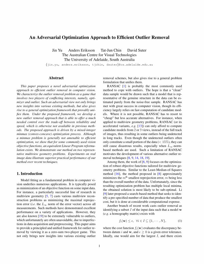
Figure 1. Behaviour of three outlier removal schemes on sample2D line-fitting data (dots). Left: the 1-slack method (2) removesonly 3 data points (circles), hence many runs are needed to cleanthe data, whereas the overly “aggressive” L1 method (3) (right)mistakenly removes many inliers. The proposed approach (center)offers a more balanced result: it is clearly more productive thanthe 1-slack method, yet not sacrificing too many inliers.

tries to minimize the objective function, whereas the inter-est of outliers is to make the minimal objective as worstas possible. Such an adversarial view can be translated toa convex-concave optimization problem. Solving it allowsus to effectively identify a set of “offending” data that areresponsible for a “bad” objective value. To identify all out-liers, one can remove this set of data, and repeat the processuntil the remaining data are clean. Fig. 1 depicts one runof the three outlier removal schemes on sample line-fittingdata with 35% of outliers. It shows that our method (cen-ter) identifies noticeably more outliers than the 1-slack ap-proach (left), yet achieving so in a less “aggressive” mannerthan the L1 approach (right). Later, we prove that the twoexisting methods are special cases of our approach.

The paper proceeds as follows: We first provide a generaldescription of our problem formulation. Sec. 3 shows howto optimally solve the resulting optimization problem. InSec. 4 we discuss related work. Experiments on real multi-view geometry data are reported in Sec. 5. Sec. 6 concludesthe paper with an outlook and discussion.

2. Problem FormulationWe introduce an adversarial problem formulation for

outlier removal, and relate our method to recent techniques.

2.1. Outlier Removal as a Minmax Problem

We view the outlier removal problem as a zero-sum gamethat involves two competing players: optimizer and outlier.The optimizer aims to find a model that achieves the min-imal objective value, whereas outliers’ strategy is to makethe minimal objective value as worse as possible. To mathe-matically formulate such a game, we first introduce a binaryvariable π ∈ {0, 1}N (All vectors are by default columnvectors.); each of its entries, denoted by πi, corresponds toa datum; πi = 1 indicates that datum i is an outlier; other-wise πi = 0. Taking into account the fact that outliers onlyconstitute part of the data, we enforce π>1 = K, where1 is a vector of all ones and K ∈ [1, N ]. We use the sum

0 0.2 0.4 0.6 0.8 1

0

0.2

0.4

0.6

0.8

1K−slack approach (K = 5)

0 0.2 0.4 0.6 0.8 1

0

0.2

0.4

0.6

0.8

1K−slack approach (K = 5)

0 0.2 0.4 0.6 0.8 1

0

0.2

0.4

0.6

0.8

1K−slack approach (K = 5)

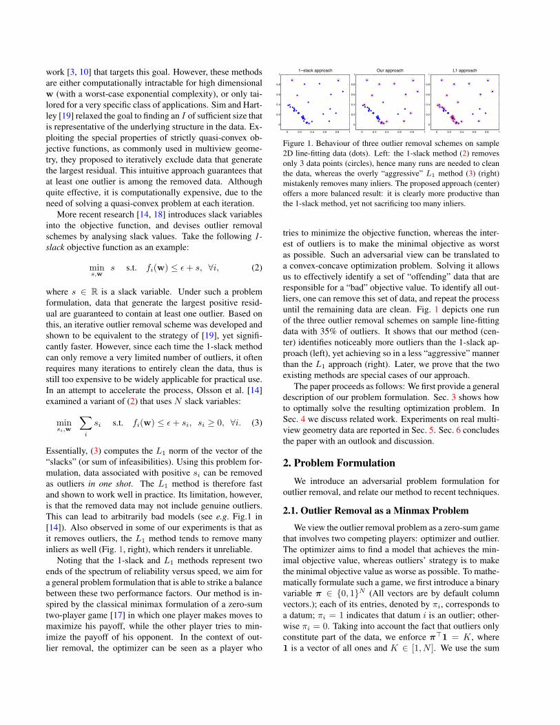
Figure 2. The model (line) and the potential outliers (circles) foundby solving (5) on various 2D line-fitting data (dots). The potentialoutliers produce larger residuals (w.r.t. the found model) than otherdata, and clearly contain genuine outliers.

of non-negative slacks to measure model fitting error. Theresulting adversarial problem takes the following form:

mins,w

maxπ

π> s (4a)

s.t. fi(w) ≤ ε+ si, si ≥ 0, ∀i (4b)

π ∈ {0, 1}N , π>1 = K, (4c)

where s ∈ RN+ collects N slacks si. The outer mins,w andinner maxπ operations characterize the strategies of the op-timizer and outliers, respectively. Denote the objective of(4) by J(s,w,π). Then, for a joint action (s,w,π), thepayoffs of the optimizer and outliers are −J(s,w,π) andrespectively, J(π, s,w). In the game equilibrium, the op-timizer minimizes the sum of the K-largest slacks, whichcan be identified by the K positive entries of π.

2.2. A Relaxed Minmax Formulation

The problem (4) seems difficult to optimize due to thepresence of the discrete constraint on π. Fortunately, thelinearity of (4) in π allows us to relax the constraint π ∈{0, 1}N to π ∈ [0, 1]N without changing the optimal ob-jective value. To see this, for the moment, let us relax thediscrete constraint to obtain the following relaxation:

mins,w

maxπ

π> s (5a)

s.t. fi(w) ≤ ε+ si, si ≥ 0, ∀i (5b)

π ∈ [0, 1]N , π>1 = K. (5c)

The inner maximization problem of (5) is simply a LinearProgram (LP). This ensures that the optimal π can be at-tained at vertices of the linear constraints on π (5c). Sincethe vertices of these constraints are integral, the optimal πis integral. The relaxation (5) is therefore an equivalent re-formulation of its mixed-integer counterpart (4).

We can see that for a given s, the optimal solution tothe inner maxπ problem can be achieved by choosing theK-largest entries of s as outliers. Denote the optimal solu-tion to (5) by (s∗,w∗,π∗). Then, for the purpose of outlierremoval, one can simply remove the data in the following

0 0.2 0.4 0.6 0.8 1

0

0.2

0.4

0.6

0.8

1K−slack approach (K = 1)

0 0.2 0.4 0.6 0.8 1

0

0.2

0.4

0.6

0.8

1K−slack approach (K = 15)

0 0.2 0.4 0.6 0.8 1

0

0.2

0.4

0.6

0.8

1K−slack approach (K = 38)

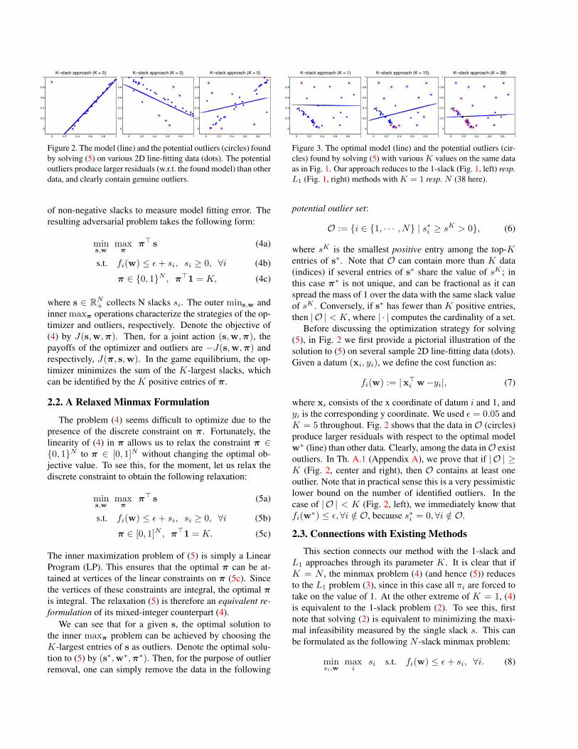
Figure 3. The optimal model (line) and the potential outliers (cir-cles) found by solving (5) with various K values on the same dataas in Fig. 1. Our approach reduces to the 1-slack (Fig. 1, left) resp.L1 (Fig. 1, right) methods with K = 1 resp. N (38 here).

potential outlier set:

O := {i ∈ {1, · · · , N} | s∗i ≥ sK > 0}, (6)

where sK is the smallest positive entry among the top-Kentries of s∗. Note that O can contain more than K data(indices) if several entries of s∗ share the value of sK ; inthis case π∗ is not unique, and can be fractional as it canspread the mass of 1 over the data with the same slack valueof sK . Conversely, if s∗ has fewer than K positive entries,then | O | < K, where | · | computes the cardinality of a set.

Before discussing the optimization strategy for solving(5), in Fig. 2 we first provide a pictorial illustration of thesolution to (5) on several sample 2D line-fitting data (dots).Given a datum (xi, yi), we define the cost function as:

fi(w) := |x>i w−yi|, (7)

where xi consists of the x coordinate of datum i and 1, andyi is the corresponding y coordinate. We used ε = 0.05 andK = 5 throughout. Fig. 2 shows that the data in O (circles)produce larger residuals with respect to the optimal modelw∗ (line) than other data. Clearly, among the data inO existoutliers. In Th. A.1 (Appendix A), we prove that if | O | ≥K (Fig. 2, center and right), then O contains at least oneoutlier. Note that in practical sense this is a very pessimisticlower bound on the number of identified outliers. In thecase of | O | < K (Fig. 2, left), we immediately know thatfi(w∗) ≤ ε,∀i /∈ O, because s∗i = 0,∀i /∈ O.

2.3. Connections with Existing Methods

This section connects our method with the 1-slack andL1 approaches through its parameter K. It is clear that ifK = N , the minmax problem (4) (and hence (5)) reducesto the L1 problem (3), since in this case all πi are forced totake on the value of 1. At the other extreme of K = 1, (4)is equivalent to the 1-slack problem (2). To see this, firstnote that solving (2) is equivalent to minimizing the maxi-mal infeasibility measured by the single slack s. This canbe formulated as the following N -slack minmax problem:

minsi,w

maxi

si s.t. fi(w) ≤ ε+ si, ∀i. (8)

If there exist outliers in the data, the maximal si for (8) mustbe positive, hence we can add the constraints: si ≥ 0,∀i to(8) without changing its optimal objective value. It is theneasy to recognize that (8) is simply (4) with K = 1.

Fig. 3 illustrates the influence of K on the solution to(5). The data in Fig. 1 were again used here. By compar-ing to Fig. 1 (left and right), we can see that our methodreduces to the 1-slack and L1 methods with K = 1 andrespectively, N . As can be seen, with different K values,models (lines) returned by solving (5) are different. The 1-slack model (left) is determined by the worst residual (i.e.the largest slack), while the L1 model (right) is influencedby the residuals of all data. These two settings overlook thefact that the size of outlier population is almost always be-tween 1 andN and it is the joint effort of this subpopulationof the data that degrades the model quality. To capture thisphenomenon, the introduction of the K parameter as in ourproblem formulation is therefore necessary. Fig. 3 (center)also shows that with an intermediate K, more “offending”data are identified than setting K = 1, while unlike theK = N case, the majority of them are indeed outliers.

Note that the three methods share one limitation, thatis, they can mistakenly remove inliers. Therefore, they arenot recommended for use on severely contaminated data,that may require many runs to clean, hence increasing thechance of removing many inliers. For this reason, all threemethods are best used at a refinement stage after a crudeRANSAC-like outlier filtering. Nevertheless, our experi-ments suggest that 1-slack and our method with an interme-diateK can still handle 15%-35% of outliers, while the per-formance of the L1 method is unstable and data-dependent.

3. An Equivalent LP Reformulation

One potential technical difficulty with the minmax for-mulation (5) is that it is generally not amenable to efficientconvex optimization. However, if the constraints in (5b) arelinear in w, we can derive an equivalent LP reformulation.This significantly simplifies the optimization.

Since the objective function (5a) is bilinear in s and π,our first step is to decouple these two terms so as to avoidintroducing non-convexity into the optimization. We do soby analysing the dual of the inner maxπ problem. Introduc-ing Lagrange multipliers α ∈ R and β ∈ RN+ , we can writethe dual of the inner maxπ problem as:

minα,β

αK + β>1 s.t. α1 + β ≥ s, β ≥ 0, (9)

where 0 denotes a column vector of all zeros. Replacingthe inner maxπ problem in (5) with (9) gives the following

Algorithm 1 Outlier Removal by Minmax Optimization1: input data and the choice of K2: output a subset I of the data such that

∃w ∈ Rd : fi(w) ≤ ε, ∀i ∈ I3: repeat4: solve (10) on the current data to obtain the optimal

solution (α∗,β∗,w∗, s∗)5: if α∗K + β∗>1 > 0 then6: construct the potential outlier set O via (6)7: remove the data collected in O8: end if9: until α∗K + β∗>1 = 0

10: optional: restore inliers from the removed data

equivalent minimization problem:

minα,β,s,w

αK + β>1 (10a)

s.t. fi(w) ≤ ε+ si, ∀i (10b)α1 + β ≥ s, β ≥ 0, s ≥ 0. (10c)

It is a convex problem if fi(w) is convex; all cost functionsconsidered in this paper are convex. Furthermore, if fi(w)is linear, then (10) is simply an LP. In this case we can rep-resent (10b) in compact matrix form as

Aj w ≤ bj + s, ∀j, (11)

where the matrix Aj ∈ RN×d and the vector bj ∈ RN con-tain the coefficients of linear constraints enforced by (10b).The values of the coefficients and the range of j are deter-mined by the exact form of the cost function fi(w). Take(7) for instance, it can be realized by two linear constraints:

x>i w ≤ yi + ε and − x>i w ≤ −yi + ε.

Expressing these constraints for all i in the matrix formof (11), we obtain two coefficient matrices: A1 :=[x>1 ; · · · ; x>N ] and A2 := −A1, with their correspondingcoefficient vectors given by b1 := [y1; · · · ; yN ] + ε1 andb2 := −[y1; · · · ; yN ] + ε1, respectively. Having solvedthe LP, one can simply sort the entries of the optimal s innon-ascending order to form the potential outlier set O (6),remove all the data in O, and repeat the process on the re-maining data until the optimal objective value of (10) re-duces to 0. Alg. 1 details our approach (named K-slack).

4. Related Work

Perhaps the closest in spirit to our paper is the work ofNguyen and Welsch [12], who tailored a maxmin formula-tion for outlier removal in least squares regression. Their

objective function takes the following form:

maxπ

minw∈Rd

∑i

πi fi(w)2 (12a)

s.t. π ∈ [0, 1]N , π>1 = K, (12b)

where fi(w) is defined as (7). To optimize (12), they firstsubstitute the inner minw problem with its closed-form so-lution so as to convert (12) to a maximization problem in πonly, which is then further reformulated as a semi-definiteprogram (SDP) for convex optimization. The resulting SDPhas (N + 1) variables and (N + 1) corresponding real sym-metric matrices of size (d+1)× (d+1) in the linear matrixinequality constraints of the SDP.

Compared to our approach, this SDP-based method isclearly less general since it restricts the cost function to be inthe least-squares form, which may not be desirable for somecomputer vision problems [4]. Moreover, the computationalcomplexity of solving the SDP reformulation of (12) via anSDP solver such as SeDuMi [20] is in the order of (N +1)2(d+ 1)2.5. This can be prohibitively expensive for highdimensional problems such as the Structure from Motionproblems considered in Sec. 5.2, where we need to estimate3D coordinates of all the observed 2D image points as wellas translation parameters of a set of cameras.

One possible remedy for the computational issue of theSDP-based method is to use our minmax formulation (5)to rewrite (12) as an equivalent but less expensive Second-Order Cone Program (SOCP). The equivalence of (5) and(12) is derived from the fact that the mins,w and maxπ op-erations in (5) are interchangeable if fi(w) is continuousand convex. With such an fi(w), the feasible region of w,as specified by (5b), is convex and closed. It is also clearthat the feasible region of s is convex and closed; and thatofπ is convex and bounded. Invoking the minimax theorem[15, Corollary 37.3.2] allows us to swap mins,w and maxπ

in (5) without changing the optimal object value. Settingε = 0 and replacing fi(w) in (5b) with the convex and con-tinuous squared cost as used in (12), we obtain an equiva-lent reformulation of (12). Squaring fi(w) in (5b) producesa set of quadratic constraints, which can be easily convertedto Second Order Cone constraints. This leads to a compu-tationally cheaper SOCP than the SDP. If further speedup ispreferred, then a linear cost function is probably more ap-propriate, as in that case one only need to solve an LP (10).

5. ExperimentsWe tested our method (K-slack, Alg. 1) on two multiview

geometry problems: Homography estimation and Structurefrom Motion (SfM) estimation with known camera rotation.We implemented our method in MATLAB with MOSEKLP solver.1 All experiments were run on a machine with

1Available from http://www.mosek.com.

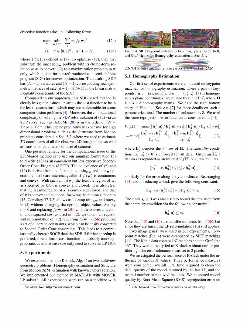
Figure 4. SIFT keypoint matches on two image pairs: Keble (left)and Graf (right), for Homography estimation in Sec. 5.1.

2.67GHz Intel quad core processors and 4 GB of RAM.

5.1. Homography Estimation

Our first set of experiments were conducted on keypointmatches for homography estimation, where a pair of key-points: u := (xi, yi, 1) and u′ := (x′i, y

′i, 1) (in homoge-

neous plane coordinates) are related by u ' Hu′, where His a 3 × 3 homography matrix. We fixed the right bottomentry of H to 1. (See e.g. [7] for more details on such aparameterization.) The number of unknowns is 8. We usedthe same reprojection error function as considered in [14]:

Vi(H) := max(|h>1 u′i /h>3 u′i−xi|, |h>2 u′i /h>3 u′i−yi|)

= max(| (h>1 −xi h

>3 ) u′i

h>3 u′i|, | (h

>2 −yi h

>3 ) u′i

h>3 u′i|), (13)

where h>j denotes the jth row of H. The cheirality condi-tion: h>3 u′i > 0 is enforced for all data. Given an H, adatum i is regarded as an inlier if Vi(H) ≤ ε, this requires

|(h>1 −xi h>3 ) u′i | ≤ εh

>3 u′i, (14)

similarly for the error along the y coordinate. Rearranging(14) and introducing a slack give the following constraint:

|(h>1 −xi h>3 ) u′i | − εh

>3 u′i ≤ si. (15)

The slack si ≥ 0 was also used to bound the deviation fromthe cheirality condition via the following constraint:

−h>3 u′i ≤ si. (16)

Note that (15) and (16) are in different forms from (5b), butsince they are linear, the LP reformulation (10) still applies.

Two image pairs2 were used in our experiments. Key-point matches (Fig. 4) were established by SIFT matching[11]. The Keble data contain 167 matches and the Graf data437. They were directly fed to K-slack without outlier pre-filtering. The error tolerance ε was set to 2 pixels.

We investigated the performance of K-slack under the in-fluence of various K values. Three performance measureswere considered: overall CPU time required to clean thedata, quality of the model returned by the last LP, and theoverall number of removed matches. We measured modelquality by Root Mean Square (RMS) reprojection error on

2Both obtained from http://www.robots.ox.ac.uk/∼vgg.

0 20 40 60 80 1000

0.5

1

1.5

K (%)

CPU

Sec

onds

KebleGraf

0 20 40 60 80 1000.5

1

1.5

2

K (%)R

MS

Erro

r

KebleGraf

0 20 40 60 80 10020

40

60

80

100

K (%)

Rem

oved

Mat

ches

(%)

KebleGraf

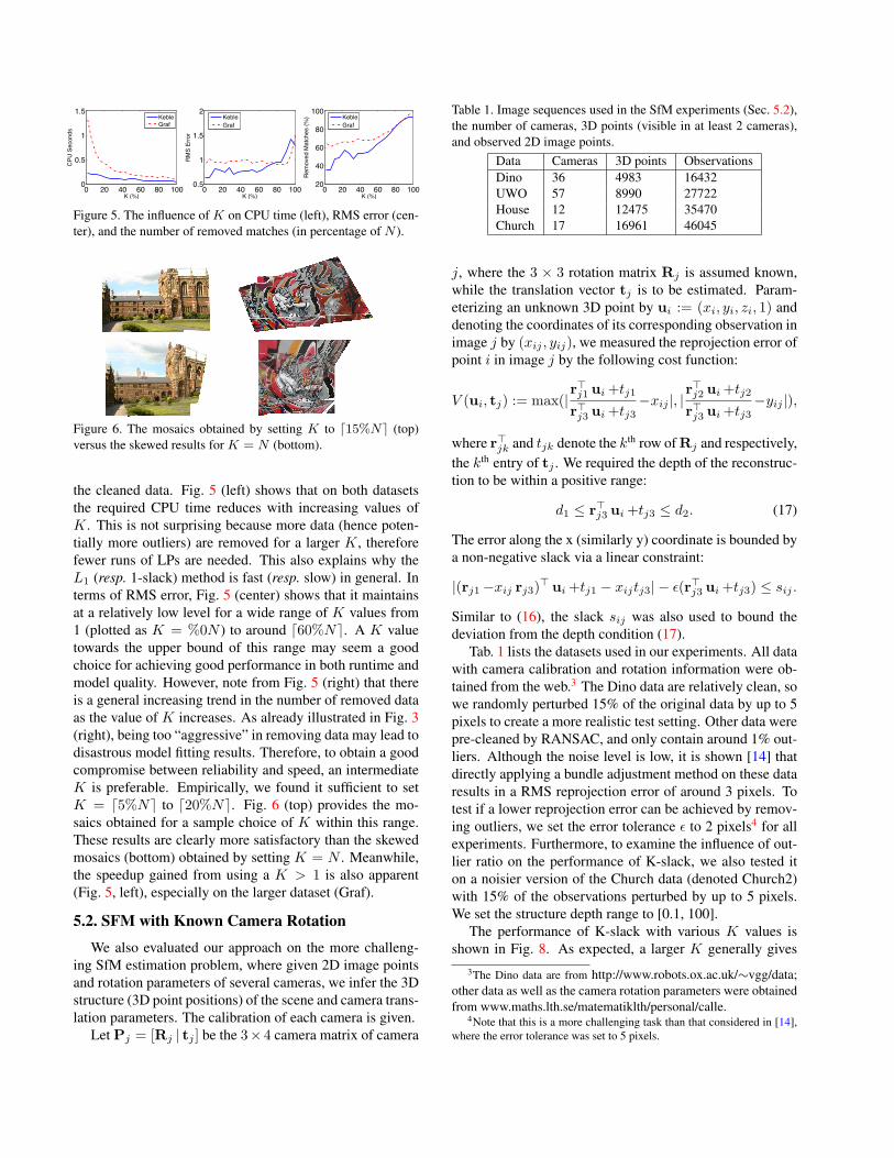
Figure 5. The influence of K on CPU time (left), RMS error (cen-ter), and the number of removed matches (in percentage of N ).

Figure 6. The mosaics obtained by setting K to d15%Ne (top)versus the skewed results for K = N (bottom).

the cleaned data. Fig. 5 (left) shows that on both datasetsthe required CPU time reduces with increasing values ofK. This is not surprising because more data (hence poten-tially more outliers) are removed for a larger K, thereforefewer runs of LPs are needed. This also explains why theL1 (resp. 1-slack) method is fast (resp. slow) in general. Interms of RMS error, Fig. 5 (center) shows that it maintainsat a relatively low level for a wide range of K values from1 (plotted as K = %0N ) to around d60%Ne. A K valuetowards the upper bound of this range may seem a goodchoice for achieving good performance in both runtime andmodel quality. However, note from Fig. 5 (right) that thereis a general increasing trend in the number of removed dataas the value of K increases. As already illustrated in Fig. 3(right), being too “aggressive” in removing data may lead todisastrous model fitting results. Therefore, to obtain a goodcompromise between reliability and speed, an intermediateK is preferable. Empirically, we found it sufficient to setK = d5%Ne to d20%Ne. Fig. 6 (top) provides the mo-saics obtained for a sample choice of K within this range.These results are clearly more satisfactory than the skewedmosaics (bottom) obtained by setting K = N . Meanwhile,the speedup gained from using a K > 1 is also apparent(Fig. 5, left), especially on the larger dataset (Graf).

5.2. SFM with Known Camera Rotation

We also evaluated our approach on the more challeng-ing SfM estimation problem, where given 2D image pointsand rotation parameters of several cameras, we infer the 3Dstructure (3D point positions) of the scene and camera trans-lation parameters. The calibration of each camera is given.

Let Pj = [Rj | tj ] be the 3× 4 camera matrix of camera

Table 1. Image sequences used in the SfM experiments (Sec. 5.2),the number of cameras, 3D points (visible in at least 2 cameras),and observed 2D image points.

Data Cameras 3D points ObservationsDino 36 4983 16432UWO 57 8990 27722House 12 12475 35470Church 17 16961 46045

j, where the 3 × 3 rotation matrix Rj is assumed known,while the translation vector tj is to be estimated. Param-eterizing an unknown 3D point by ui := (xi, yi, zi, 1) anddenoting the coordinates of its corresponding observation inimage j by (xij , yij), we measured the reprojection error ofpoint i in image j by the following cost function:

V (ui, tj) := max(|r>j1 ui +tj1r>j3 ui +tj3

−xij |, |r>j2 ui +tj2r>j3 ui +tj3

−yij |),

where r>jk and tjk denote the kth row of Rj and respectively,the kth entry of tj . We required the depth of the reconstruc-tion to be within a positive range:

d1 ≤ r>j3 ui +tj3 ≤ d2. (17)

The error along the x (similarly y) coordinate is bounded bya non-negative slack via a linear constraint:

|(rj1−xij rj3)> ui +tj1 − xijtj3| − ε(r>j3 ui +tj3) ≤ sij .

Similar to (16), the slack sij was also used to bound thedeviation from the depth condition (17).

Tab. 1 lists the datasets used in our experiments. All datawith camera calibration and rotation information were ob-tained from the web.3 The Dino data are relatively clean, sowe randomly perturbed 15% of the original data by up to 5pixels to create a more realistic test setting. Other data werepre-cleaned by RANSAC, and only contain around 1% out-liers. Although the noise level is low, it is shown [14] thatdirectly applying a bundle adjustment method on these dataresults in a RMS reprojection error of around 3 pixels. Totest if a lower reprojection error can be achieved by remov-ing outliers, we set the error tolerance ε to 2 pixels4 for allexperiments. Furthermore, to examine the influence of out-lier ratio on the performance of K-slack, we also tested iton a noisier version of the Church data (denoted Church2)with 15% of the observations perturbed by up to 5 pixels.We set the structure depth range to [0.1, 100].

The performance of K-slack with various K values isshown in Fig. 8. As expected, a larger K generally gives

3The Dino data are from http://www.robots.ox.ac.uk/∼vgg/data;other data as well as the camera rotation parameters were obtainedfrom www.maths.lth.se/matematiklth/personal/calle.

4Note that this is a more challenging task than that considered in [14],where the error tolerance was set to 5 pixels.

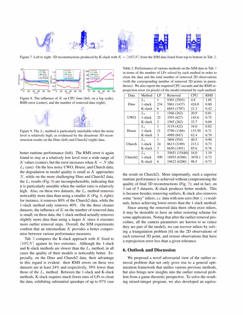
Figure 7. Left to right: 3D reconstructions produced by K-slack with K = d10%Ne from the SfM data listed from top to bottom in Tab. 2.

0 20 40 60 80 100100

102

104

K (%)

CPU

Sec

onds

DinoUWOHouseChurchChurch2

0 20 40 60 80 1000.20.40.60.8

11.2

K (%)

RM

S Er

ror

DinoUWOHouseChurchChurch2

0 20 40 60 80 100020406080

100

K (%)

Rem

oved

Obs

erva

tions

(%)

DinoUWOHouseChurchChurch2

Figure 8. The influence of K on CPU time (left, on a log scale),RMS error (center), and the number of removed data (right).

Figure 9. The L1 method is particularly unreliable when the noiselevel is relatively high, as evidenced by the disastrous 3D recon-struction results on the Dino (left) and Church2 (right) data.

better runtime performance (left). The RMS error is againfound to stay at a relatively low level over a wide range ofK values (center), but the error increases whenK = N (theL1 case). On the less noisy UWO, House, and Church data,the degradation in model quality is small as K approachesN , while on the more challenging Dino and Church2 data,the L1 results (Fig. 9) are incomprehensible, indicating thatit is particularly unstable when the outlier ratio is relativelyhigh. Also, on these two datasets, the L1 method removesnoticeably more data than using a smaller K (Fig. 8, right);for instance, it removes 80% of the Church2 data, while the1-slack method only removes 40%. On the three cleanerdatasets, the influence of K on the number of removed datais small; on these data, the 1-slack method actually removesslightly more data than using a larger K since it executesmore outlier removal steps. Overall, the SfM experimentsconfirm that an intermediate K provides a better compro-mise between various performance measures.

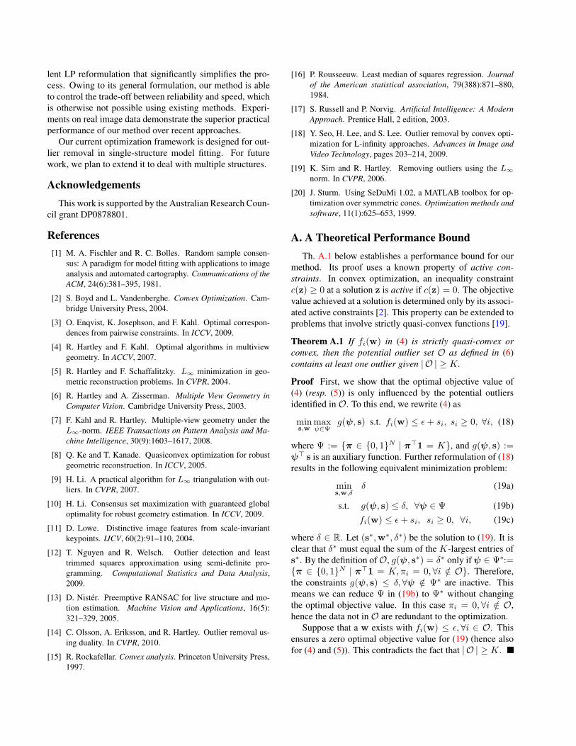
Tab. 2 compares the K-slack approach with K fixed tod10%Ne against its two extremes. Although the 1-slackand K-slack methods are slower than the L1 method, in allcases the quality of their models is noticeably better. Es-pecially, on the Dino and Church2 data, their advantagein this regard is evident: their RMS errors on these twodatasets are at least 24% and respectively, 39% lower thanthose of the L1 method. Between the 1-slack and K-slackmethods, K-slack requires much fewer runs of LPs to cleanthe data, exhibiting substantial speedups of up to 97% (see

Table 2. Performance of various methods on the SfM data in Tab. 1in terms of the number of LPs solved by each method in order toclean the data and the total number of removed 2D observations(with the corresponding number of removed 3D points in paren-theses). We also report the required CPU seconds and the RMS re-projection error (in pixels) of the model returned by each method.

Data Method LP Removed CPU RMS

DinoL1 1 9301 (2503) 4.8 1.051-slack 234 5861 (1437) 424.0 0.80K-slack 6 6843 (1707) 21.3 0.42

UWOL1 1 1566 (262) 20.9 0.811-slack 25 3593 (627) 145.6 0.75K-slack 2 1565 (262) 33.7 0.69

HouseL1 1 3119 (422) 34.0 0.821-slack 21 5790 (1166) 133.50 0.71K-slack 3 4989 (847) 62.4 0.70

ChurchL1 1 3804 (554) 40.5 0.901-slack 24 8613 (2189) 213.1 0.73K-slack 3 6650 (1491) 85.6 0.76

Church2L1 1 35651 (15440) 16.0 1.191-slack 590 18955 (6380) 3078.1 0.72K-slack 6 19622 (6200) 98.5 0.73

the result on Church2). More importantly, such a superiorruntime performance is achieved without compromising thequality of final 3D reconstructions (Fig. 7); and in fact, on3 out of 5 datasets, K-slack produces better models. Thisis because besides removing outliers, K-slack also removessome “noisy” inliers, i.e. data with non-zero (but≤ ε) resid-uals, hence achieving lower errors than the 1-slack method.

Since among the removed data there often exist inliers,it may be desirable to have an inlier restoring scheme forsome applications. Noting that after the outlier removal pro-cedure, all the camera parameters are known to us (sincethey are part of the model), we can recover inliers by solv-ing a triangulation problem [6] on the 2D observations ofeach removed 3D point, and restore observations that havea reprojection error less than a given tolerance.

6. Outlook and DiscussionWe proposed a novel adversarial view of the outlier re-

moval problem that not only gives rise to a general opti-mization framework that unifies various previous methods,but also brings new insights into the outlier removal prob-lem from a game-theoretic perspective. To solve the result-ing mixed-integer program, we also developed an equiva-

lent LP reformulation that significantly simplifies the pro-cess. Owing to its general formulation, our method is ableto control the trade-off between reliability and speed, whichis otherwise not possible using existing methods. Experi-ments on real image data demonstrate the superior practicalperformance of our method over recent approaches.

Our current optimization framework is designed for out-lier removal in single-structure model fitting. For futurework, we plan to extend it to deal with multiple structures.

AcknowledgementsThis work is supported by the Australian Research Coun-

cil grant DP0878801.

References[1] M. A. Fischler and R. C. Bolles. Random sample consen-

sus: A paradigm for model fitting with applications to imageanalysis and automated cartography. Communications of theACM, 24(6):381–395, 1981.

[2] S. Boyd and L. Vandenberghe. Convex Optimization. Cam-bridge University Press, 2004.

[3] O. Enqvist, K. Josephson, and F. Kahl. Optimal correspon-dences from pairwise constraints. In ICCV, 2009.

[4] R. Hartley and F. Kahl. Optimal algorithms in multiviewgeometry. In ACCV, 2007.

[5] R. Hartley and F. Schaffalitzky. L∞ minimization in geo-metric reconstruction problems. In CVPR, 2004.

[6] R. Hartley and A. Zisserman. Multiple View Geometry inComputer Vision. Cambridge University Press, 2003.

[7] F. Kahl and R. Hartley. Multiple-view geometry under theL∞-norm. IEEE Transactions on Pattern Analysis and Ma-chine Intelligence, 30(9):1603–1617, 2008.

[8] Q. Ke and T. Kanade. Quasiconvex optimization for robustgeometric reconstruction. In ICCV, 2005.

[9] H. Li. A practical algorithm for L∞ triangulation with out-liers. In CVPR, 2007.

[10] H. Li. Consensus set maximization with guaranteed globaloptimality for robust geometry estimation. In ICCV, 2009.

[11] D. Lowe. Distinctive image features from scale-invariantkeypoints. IJCV, 60(2):91–110, 2004.

[12] T. Nguyen and R. Welsch. Outlier detection and leasttrimmed squares approximation using semi-definite pro-gramming. Computational Statistics and Data Analysis,2009.

[13] D. Nister. Preemptive RANSAC for live structure and mo-tion estimation. Machine Vision and Applications, 16(5):321–329, 2005.

[14] C. Olsson, A. Eriksson, and R. Hartley. Outlier removal us-ing duality. In CVPR, 2010.

[15] R. Rockafellar. Convex analysis. Princeton University Press,1997.

[16] P. Rousseeuw. Least median of squares regression. Journalof the American statistical association, 79(388):871–880,1984.

[17] S. Russell and P. Norvig. Artificial Intelligence: A ModernApproach. Prentice Hall, 2 edition, 2003.

[18] Y. Seo, H. Lee, and S. Lee. Outlier removal by convex opti-mization for L-infinity approaches. Advances in Image andVideo Technology, pages 203–214, 2009.

[19] K. Sim and R. Hartley. Removing outliers using the L∞norm. In CVPR, 2006.

[20] J. Sturm. Using SeDuMi 1.02, a MATLAB toolbox for op-timization over symmetric cones. Optimization methods andsoftware, 11(1):625–653, 1999.

A. A Theoretical Performance BoundTh. A.1 below establishes a performance bound for our

method. Its proof uses a known property of active con-straints. In convex optimization, an inequality constraintc(z) ≥ 0 at a solution z is active if c(z) = 0. The objectivevalue achieved at a solution is determined only by its associ-ated active constraints [2]. This property can be extended toproblems that involve strictly quasi-convex functions [19].

Theorem A.1 If fi(w) in (4) is strictly quasi-convex orconvex, then the potential outlier set O as defined in (6)contains at least one outlier given | O | ≥ K.

Proof First, we show that the optimal objective value of(4) (resp. (5)) is only influenced by the potential outliersidentified in O. To this end, we rewrite (4) as

mins,w

maxψ∈Ψ

g(ψ, s) s.t. fi(w) ≤ ε+ si, si ≥ 0, ∀i, (18)

where Ψ := {π ∈ {0, 1}N | π>1 = K}, and g(ψ, s) :=ψ> s is an auxiliary function. Further reformulation of (18)results in the following equivalent minimization problem:

mins,w,δ

δ (19a)

s.t. g(ψ, s) ≤ δ, ∀ψ ∈ Ψ (19b)fi(w) ≤ ε+ si, si ≥ 0, ∀i, (19c)

where δ ∈ R. Let (s∗,w∗, δ∗) be the solution to (19). It isclear that δ∗ must equal the sum of the K-largest entries ofs∗. By the definition ofO, g(ψ, s∗) = δ∗ only ifψ ∈ Ψ∗:={π ∈ {0, 1}N | π>1 = K,πi = 0,∀i /∈ O}. Therefore,the constraints g(ψ, s) ≤ δ, ∀ψ /∈ Ψ∗ are inactive. Thismeans we can reduce Ψ in (19b) to Ψ∗ without changingthe optimal objective value. In this case πi = 0,∀i /∈ O,hence the data not in O are redundant to the optimization.

Suppose that a w exists with fi(w) ≤ ε, ∀i ∈ O. Thisensures a zero optimal objective value for (19) (hence alsofor (4) and (5)). This contradicts the fact that | O | ≥ K.