An Affine Invariant k-Nearest Neighbor

Regression Estimate

Gerard Biau1

Universite Pierre et Marie Curie2 & Ecole Normale Superieure3, France

gerard.biau@upmc.fr

Luc DevroyeMcGill University, Canada4

lucdevroye@gmail.com

Vida DujmovicCarleton University, Canada5

vida@scs.carleton.ca

Adam KrzyzakConcordia University, Canada6

krzyzak@cs.concordia.ca

Abstract

We design a data-dependent metric in Rd and use it to define the k-

nearest neighbors of a given point. Our metric is invariant under all

affine transformations. We show that, with this metric, the standard

k-nearest neighbor regression estimate is asymptotically consistent un-

der the usual conditions on k, and minimal requirements on the input

data.

Index Terms — Nonparametric estimation, Regression function esti-

mation, Affine invariance, Nearest neighbor methods, Mathematical

statistics.

2010 Mathematics Subject Classification: 62G08, 62G05, 62G20.

1Corresponding author.2Research partially supported by the French National Research Agency under grant

ANR-09-BLAN-0051-02 “CLARA”.3Research carried out within the INRIA project “CLASSIC” hosted by Ecole Normale

Superieure and CNRS.4Research sponsored by NSERC Grant A3456 and FQRNT Grant 90-ER-0291.5Research sponsored by NSERC Grant RGPIN 402438-2011.6Research sponsored by NSERC Grant N00118.

1

1 Introduction

The prediction error of standard nonparametric regression methods may becritically affected by a linear transformation of the coordinate axes. It istypically the case for the popular k-nearest neighbor (k-NN) predictor (Fixand Hodges [11, 12], Cover and Hart [7], Cover [5, 6]), where a mere rescal-ing of the coordinate axes has a serious impact on the capabilities of thisestimate. This is clearly an undesirable feature, especially in applicationswhere the data measurements represent physically different quantities, suchas temperature, blood pressure, cholesterol level, and the age of the patient.In this example, a simple change in, say, the unit measure of the tempera-ture parameter will lead to totally different results, and will thus force thestatistician to use a somewhat arbitrary preprocessing step prior to the k-NNestimation process. Furthermore, in several practical implementations, onewould like, for physical or economical reasons, to supply the freshly collecteddata to some machine without preprocessing.

In this paper, we discuss a variation of the k-NN regression estimate whosedefinition is not affected by affine transformations of the coordinate axes.Such a modification could save the user a subjective preprocessing step andwould save the manufacturer the trouble of adding input specifications.

The data set we have collected can be regarded as a collection of inde-pendent and identically distributed R

d × R-valued random variables Dn ={(X1, Y1), . . . , (Xn, Yn)}, independent of and with the same distribution as ageneric pair (X, Y ) satisfying E|Y | < ∞. The space Rd is equipped with thestandard Euclidean norm ‖.‖. For fixed x ∈ R

d, our goal is to estimate theregression function r(x) = E[Y |X = x] using the data Dn. In this context,the usual k-NN regression estimate takes the form

rn(x;Dn) =1

kn

kn∑

i=1

Y(i)(x),

where (X(1)(x), Y(1)(x)), . . . , (X(n)(x), Y(n)(x)) is a reordering of the data ac-cording to increasing distances ‖Xi − x‖ of the Xi’s to x. (If distance tiesoccur, a tie-breaking strategy must be defined. For example, if ‖Xi − x‖ =‖Xj − x‖, Xi may be declared “closer” if i < j, i.e., the tie-breaking isdone by indices.) For simplicity, we will suppress Dn in the notation andwrite rn(x) instead of rn(x;Dn). Stone [37] showed that, for all p ≥ 1,E|rn(X)−r(X)|p → 0 for all possible distributions of (X, Y ) with E|Y |p < ∞,whenever kn → ∞ and kn/n → 0 as n → ∞. Thus, the k-NN estimate be-haves asymptotically well, without exceptions. This property is called Lp

universal consistency.

2

Clearly, any affine transformation of the coordinate axes influences the k-NN estimate through the norm ‖.‖, thereby illuminating an unpleasant faceof the procedure. To illustrate this remark, assume that a nontrivial affinetransformation T : z 7→ Az+b (that is, a nonsingular linear transformation Afollowed by a translation b) is applied to both x and X1, . . . ,Xn. Examplesinclude any number of combinations of rotations, translations, and linearrescalings. Denote by D′

n = (T (X1), Y1), . . . , (T (Xn), Yn) the transformedsample. Then, for such a function T , one has rn(x;Dn) 6= rn(T (x);D

′n) in

general, whereas r(X) = E[Y |T (X)] since T is bijective. Thus, to continueour discussion, we are looking in essence for a regression estimate rn withthe following property:

rn(x;Dn) = rn(T (x);D′n). (1.1)

We call rn affine invariant. Affine invariance is indeed a very strong buthighly desirable property. In R

d, in the context of k-NN estimates, it sufficesto be able to define an affine invariant distance measure, which is necessarilydata-dependent. With this objective in mind, we develop in the next sectionan estimation procedure featuring (1.1) which in form coincides with the k-NN estimate, and establish its consistency in Section 3. Proofs of the mosttechnical results are gathered in Section 4.

It should be stressed that what we are after in this article is an estimate of rwhich is invariant by an affine transformation of both the query point x andthe original regressors X1, . . . ,Xn. When the sole regressors are subject tosuch a transformation, it is then more natural to talk of “affine equivariant”regression estimates rather than of “affine invariant” ones; this is more in linewith the terminology used, for example, in Ollila, Hettmansperger, and Oja[28] and Ollila, Oja, and Koivunen [29]. These affine invariance and affineequivariance requirements, however, are strictly equivalent.

There have been many attempts in the nonparametric literature to achieveaffine invariance. One of the most natural ones relates to the so-calledtransformation-retransformation proposed by Chakraborty, Chaudhuri, andOja [3]. That method and many variants have been discussed in texts such as[9] and [17] for pattern recognition and regression, respectively, but they havealso been used in kernel density estimation (see, e.g., Samanta [36]). It isworth noting that, computational issues aside, the transformation step (i.e.,premultiplication of the regressors by M−1

n , where Mn is an affine equivariantscatter estimate) may be based on a statistic Mn that does not require finite-ness of any moment. A typical example is the scatter estimate proposed inTyler [38] or Hettmansperger and Randles [20]. Rather, our procedure takes

3

ideas from the classical nonparametric literature using concepts such as mul-tivariate ranks. It is close in spirit to the approach of Paindaveine and VanBever [31], who introduce a class of depth-based classification proceduresthat are of a nearest neighbor nature.

There are also attempts at getting invariance to other transformations. Themost important concept here is that of invariance under monotone transfor-mations of the coordinate axes. In particular, any strategy that uses only thecoordinatewise ranks of the Xi’s achieves this. The onus, then, is to showconsistency of the methods under the most general conditions possible. Forexample, using an Lp norm on the d-vectors of differences between ranks,one can show that the classical k-NN regression function estimate is univer-sally consistent in the sense of Stone [37]. This was observed by Olshen [30],and shown by Devroye [8] (see also Gordon and Olshen [15, 16], Devroyeand Krzyzak [10], and Biau and Devroye [2] for related works). Rules basedupon statistically equivalent blocks (see, e.g., Anderson [1], Quesenberry andGessaman [34], Gessaman [13], Gessaman and Gessaman [14], and Devroye,Gyorfi, and Lugosi [9, Section 21.4]) are other important examples of re-gression methods invariant with respect to monotone transformations of thecoordinate axes. These methods and their generalizations partition the spacewith sets that contain a fixed number of data points each.

It would be interesting to consider in a future paper the possibility of morph-ing the input space in more general ways than those suggested in the previousfew paragraphs of the present article. It should be possible, in principle, todefine appropriate metrics to obtain invariance for interesting large classesof nonlinear transformations, and show consistent asymptotic behaviors.

2 An affine invariant k-NN estimate

The k-NN estimate we are discussing is based upon the notion of empiricaldistance. Throughout, we assume that the distribution of X is absolutelycontinuous with respect to the Lebesgue measure on R

d and that n ≥ d.Because of this density assumption, any collection Xi1, . . . ,Xid (1 ≤ i1 <i2 < . . . < id ≤ n) of d points among X1, . . . ,Xn are in general positionwith probability 1. Consequently, there exists with probability 1 a uniquehyperplane in R

d containing these d random points, and we denote it byH(Xi1 , . . . ,Xid).

With this notation, the empirical distance between d-vectors x and x′ is

4

defined as

ρn(x,x′) =

∑

1≤i1<...<id≤n

1{segment (x,x′) intersects the hyperplane H(Xi1,...,Xid

)}.

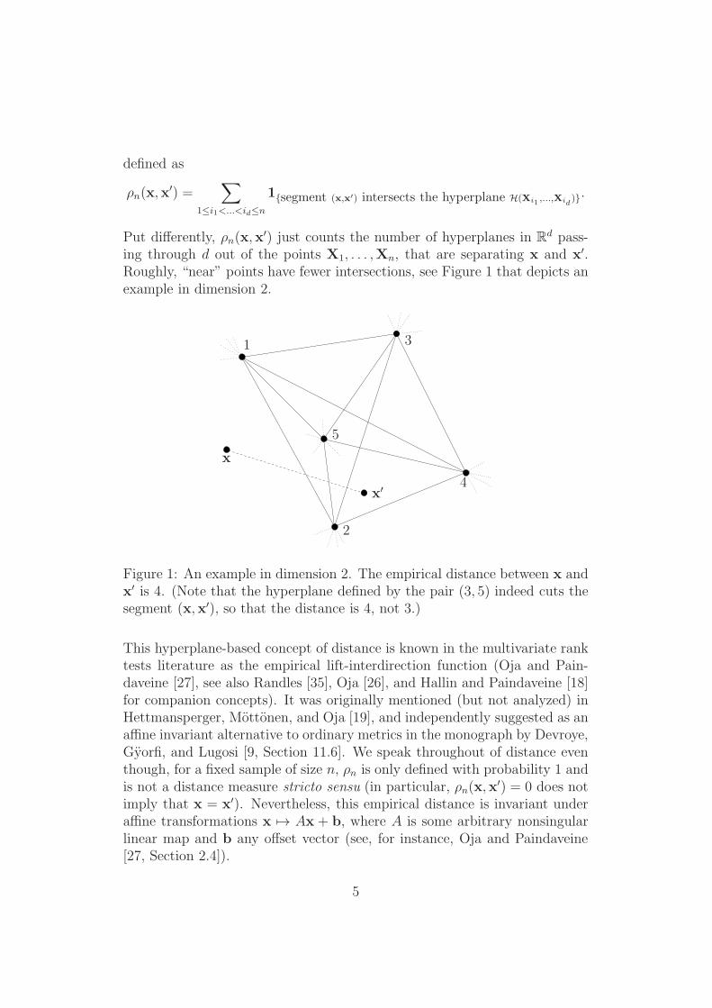
Put differently, ρn(x,x′) just counts the number of hyperplanes in R

d pass-ing through d out of the points X1, . . . ,Xn, that are separating x and x′.Roughly, “near” points have fewer intersections, see Figure 1 that depicts anexample in dimension 2.

1

2

3

4

5

x′

x

Figure 1: An example in dimension 2. The empirical distance between x andx′ is 4. (Note that the hyperplane defined by the pair (3, 5) indeed cuts thesegment (x,x′), so that the distance is 4, not 3.)

This hyperplane-based concept of distance is known in the multivariate ranktests literature as the empirical lift-interdirection function (Oja and Pain-daveine [27], see also Randles [35], Oja [26], and Hallin and Paindaveine [18]for companion concepts). It was originally mentioned (but not analyzed) inHettmansperger, Mottonen, and Oja [19], and independently suggested as anaffine invariant alternative to ordinary metrics in the monograph by Devroye,Gyorfi, and Lugosi [9, Section 11.6]. We speak throughout of distance eventhough, for a fixed sample of size n, ρn is only defined with probability 1 andis not a distance measure stricto sensu (in particular, ρn(x,x

′) = 0 does notimply that x = x′). Nevertheless, this empirical distance is invariant underaffine transformations x 7→ Ax + b, where A is some arbitrary nonsingularlinear map and b any offset vector (see, for instance, Oja and Paindaveine[27, Section 2.4]).

5

Now, fix x ∈ Rd and let ρn(x,Xi) be the empirical distance between x and

some observation Xi in the sample X1, . . . ,Xn. (That is, the number ofhyperplanes in R

d passing through d out of the observations X1, . . . ,Xn,that are cutting the segment (x,Xi)). In this context, the k-NN estimate weare considering still takes the familiar form

rn(x) =1

kn

kn∑

i=1

Y(i)(x),

with the important difference that now the data set (X1, Y1), . . . , (Xn, Yn) isreordered according to increasing values of the empirical distances ρn(x,Xi),not the original Euclidean metric. By construction, the estimate rn hasthe desired affine invariance property and, moreover, it coincides with thestandard (Euclidean) estimate in dimension d = 1. In the next section, weprove the following theorem. The distribution of the random variable X isdenoted by µ.

Theorem 2.1 (Pointwise Lp consistency) Assume that X has a proba-

bility density, that Y is bounded, and that the regression function r is µ-almost surely continuous. Then, for µ-almost all x ∈ R

d and all p ≥ 1, ifkn → ∞ and kn/n → 0,

E |rn(x)− r(x)|p → 0 as n → ∞.

The following corollary is a consequence of Theorem 2.1 and the Lebesgue’sdominated convergence theorem.

Corollary 2.1 (Global Lp consistency) Assume that X has a probability

density, that Y is bounded, and that the regression function r is µ-almost

surely continuous. Then, for all p ≥ 1, if kn → ∞ and kn/n → 0,

E |rn(X)− r(X)|p → 0 as n → ∞.

The conditions of Stone’s universal consistency theorem given in [37] are notfulfilled for our estimate. For the standard nearest neighbor estimate, a keyresult used in the consistency proof by Stone is that a given data point cannotbe the nearest neighbor of more than a constant number (say, 3d) of otherpoints. Such a universal constant does not exist after our transformation isapplied. That means that a single data point can have a large influence onthe regression function estimate. While this by itself does not imply thatthe estimate is not universally consistent, it certainly indicates that any suchproof will require new insights. The addition of two smoothness constraints,

6

namely that X has a density (without, however, imposing any continuityconditions on the density itself) and that r is µ-almost surely continuous, issufficient.

The complexity of our procedure in terms of sample size n and dimension dis quite high. There are

(

nd

)

possible choices of hyperplanes through d points.This collection of hyperplanes defines an arrangement, or partition of R

d

into polytopal regions, also called cells or chambers. Within each region, thedistance to each data point is constant, and thus, a preprocessing step mightconsist of setting up a data structure for determining to which cell a givenpoint x ∈ R

d belongs: This is called the point location problem. Meiser [24]showed that such a data structure exists with the following properties: (i)it takes space O(nd+ε) for any fixed ε > 0, and (ii) point location can beperformed in O(log n) time. Chazelle’s cuttings [4] improve (i) to O(nd).Chazelle’s processing time for setting up the data structure is O(nd). Still inthe preprocessing step, one can determine for each cell in the arrangement thedistances to all n data points: This can be done by walking across the graphof cells or by brute force. When done naively, the overall set-up complexity isO(n2d+1). For each cell, one might keep a pointer to the k nearest neighbors.Therefore, once set up, the computation of the regression function estimatetakes merely O(log n) time for point location, and O(k) time for retrievingthe k nearest neighbors.

One could envisage a reduction in the complexity by defining the distancesnot in terms of all hyperplanes that cut a line segment, but in terms ofthe number of randomly drawn hyperplanes that make such a cut, wherethe number of random draws is now a carefully selected number. By theconcentration of binomial random variables, such random estimates of thedistances are expected to work well, while keeping the complexity reasonable.This idea will be explored elsewhere.

3 Proof of the theorem

Recall, since X has a probability density with respect to the Lebesgue mea-sure on R

d, that any collection Xi1 , . . . ,Xid (1 ≤ i1 < i2 < . . . < id ≤ n) ofd points among X1, . . . ,Xn defines with probability 1 a unique hyperplaneH(Xi1 , . . . ,Xid) in R

d. Thus, in the sequel, since no confusion is possible, wewill freely refer to “the hyperplane H(Xi1, . . . ,Xid) defined by Xi1, . . . ,Xid”without further explicit mention of the probability 1 event.

Let us first fix some useful notation. The distribution of the random variableX is denoted by µ and its density with respect to the Lebesgue measure is

7

denoted by f . For every ε > 0, we let Bx,ε = {y ∈ Rd : ‖y − x‖ ≤ ε} be

the closed Euclidean ball with center at x and radius ε. We write Ac for thecomplement of a subset A of Rd. For two random variables Z1 and Z2, thenotation

Z1 ≤st Z2

means that Z1 is stochastically dominated by Z2, that is, for all t ∈ R,

P{Z1 > t} ≤ P{Z2 > t}.

Our first goal is to show that for µ-almost all x, as kn/n → 0, the quantitymaxi=1,...,kn ‖X(i)(x)− x‖ converges to 0 in probability, i.e., for every ε > 0,

limn→∞

P

{

maxi=1,...,kn

‖X(i)(x)− x‖ > ε

}

= 0. (3.1)

So, fix such a positive ε. Let δ be a real number in (0, ε) and γn be a positivereal number (eventually function of x and ε) to be determined later. Toprove identity (3.1), we use the following decomposition, which is valid forall x ∈ R

d:

P

{

maxi=1,...,kn

‖X(i)(x)− x‖ > ε

}

≤ P

mini=1,...,nXi∈Bc

x,ε

ρn(x,Xi) < γn

+ P

maxi=1,...,nXi∈B

x,δ

ρn(x,Xi) ≥ γn

+ P {Card {i = 1, . . . , n : ‖Xi − x‖ ≤ δ} < kn}

:= A+B+C. (3.2)

The convergence to 0 of each of the three terms above—from which identity(3.1) immediately follows—are separately analyzed in the next three para-graphs.

Analysis of A. As for now, taking an affine geometry point of view, wekeep x fixed and see it as the origin of the space. Recall that each point inthe Euclidean space R

d (with the origin at x) may be described by its hy-perspherical coordinates (see, e.g., Miller [25, Chapter 1]), which consist ofa nonnegative radial coordinate r and d− 1 angular coordinates θ1, . . . , θd−1,

8

where θd−1 ranges over [0, 2π) and the other angles range over [0, π] (adap-tation of this definition to the cases d = 1 and d = 2 is clear). For a(d−1)-dimensional vector Θ = (θ1, . . . , θd−1) of hyperspherical angles, we letBx,ε(Θ) be the unique closed ball anchored at x in the direction Θ and withdiameter ε (see Figure 2 which depicts an illustration in dimension 2). Wealso let Lx(Θ) be the axis defined by x and the direction Θ, and let as wellSx,ε(Θ) be the open segment obtained as the intersection of Lx(Θ) and theinterior of Bx,ε(Θ).

x

Θ

ε2N2

x,ε(Θ)

N1x,ε(Θ)

R2x,ε(Θ)

R1x,ε(Θ)

Sx,ε(Θ)

Lx(Θ)

Figure 2: The ball Bx,ε(Θ) and related notation. Illustration in dimension 2.

Next, for fixed x, ε and Θ, we split the ball Bx,ε(Θ) into 2d−1 disjoint regions

R1x,ε(Θ), . . . ,R2d−1

x,ε (Θ) as follows. First, the Euclidean space Rd is sequen-

tially divided into 2d−1 symmetric quadrants rotating around the axis Lx(Θ)(boundary equalities are broken arbitrarily). Next, each region Rj

x,ε(Θ) isobtained as the intersection of one of the 2d−1 quadrants and the ball Bx,ε(Θ).

The numbers of sample points falling in each of these regions are denotedhereafter by N1

x,ε(Θ), . . . , N2d−1

x,ε (Θ) (see Figure 2). Letting finally Vd be thevolume of the unit d-dimensional Euclidean ball, we are now in a position tocontrol the first term of inequality (3.2).

Proposition 3.1 For µ-almost all x ∈ Rd and all ε > 0 small enough,

P

mini=1,...,nXi∈Bc

x,ε

ρn(x,Xi) < γn

→ 0 as n → ∞,

9

provided

γn = nd

(

Vd

22d+1εdf(x)

)2d−1

.

Proof of Proposition 3.1 Set

px,ε = minj=1,...,2d−1

infΘ

µ{

Rjx,ε(Θ)

}

,

where the infimum is taken over all possible hyperspherical angles Θ. Weknow, according to technical Lemma 4.1, that for µ-almost all x and allε > 0 small enough,

px,ε ≥Vd

22dεdf(x) > 0. (3.3)

Thus, in the rest of the proof, we fix such an x and assume that ε is smallenough so that the inequalities above are satisfied.

Let X⋆ be defined as the intersection of the line (x,X) with Bx,ε, and let Θ⋆

be the (random) hyperspherical angle corresponding to X⋆ (see Figure 3 foran example in dimension 2).

x

X

X⋆

ε

N2x,ε(Θ

⋆)

N1x,ε(Θ

⋆)Θ⋆

Figure 3: The ball Bx,ε(Θ⋆) in dimension 2.

Denote by Nx,ε(Θ⋆) the number of hyperplanes passing through d out of the

10

observations X1, . . . ,Xn and cutting the segment Sx,ε(Θ⋆). We have

P

mini=1,...,nXi∈Bc

x,ε

ρn(x,Xi) < γn

≤ nP {ρn(x,X⋆) < γn}

= nP {Nx,ε(Θ⋆) < γn}

≤ nP

{

N1x,ε(Θ

⋆) . . .N2d−1

x,ε (Θ⋆)

n2d−1−d< γn

}

,

where the last inequality follows from technical Lemma 4.2. Thus,

P

mini=1,...,nXi∈Bc

x,ε

ρn(x,Xi) < γn

≤ n

2d−1∑

j=1

P

{

N jx,ε(Θ

⋆) <(

γnn2d−1−d

)1/2d−1}

= n

2d−1∑

j=1

P

{

N jx,ε(Θ

⋆) < γ1/2d−1

n n1−d/2d−1}

.

Clearly, conditionally on Θ⋆, each N jx,ε(Θ

⋆) satisfies

Binomial (n, px,ε) ≤st Njx,ε(Θ

⋆)

and consequently, by inequality (3.3),

Binomial

(

n,Vd

22dεdf(x)

)

≤st Njx,ε(Θ

⋆).

Thus, for each j = 1, . . . , 2d−1, by Hoeffding’s inequality for binomial randomvariables (Hoeffding [21]), we are led to

P

{

N jx,ε(Θ

⋆) < γ1/2d−1

n n1−d/2d−1}

= E

[

P

{

N jx,ε(Θ

⋆) < γ1/2d−1

n n1−d/2d−1

|Θ⋆}]

≤ exp

[

−2

(

γ1/2d−1

n n1−d/2d−1

− nVd

22dεdf(x)

)2

/n

]

as soon as γ1/2d−1

n n1−d/2d−1< n Vd

22dεdf(x). Therefore, taking

γn = nd

(

Vd

22d+1εdf(x)

)2d−1

,

11

we obtain

P

mini=1,...,nXi∈Bc

x,ε

ρn(x,Xi) < γn

≤ 2d−1n exp

[

−n

(

Vd

22dεdf(x)

)2

/2

]

.

The upper bound goes to 0 as n → ∞. �

Analysis of B. Consistency of the second term in inequality (3.2) is es-tablished in the following proposition.

Proposition 3.2 For µ-almost all x ∈ Rd, all ε > 0 and all δ > 0 small

enough,

P

maxi=1,...,nXi∈B

x,δ

ρn(x,Xi) ≥ γn

→ 0 as n → ∞,

provided

γn = nd

(

Vd

22d+1εdf(x)

)2d−1

. (3.4)

Proof of Proposition 3.2 Fix x in a set of µ-measure 1 such that f(x) > 0and denote by Nx,δ the number of hyperplanes that cut the ball Bx,δ. Clearly,

P

maxi=1,...,nXi∈B

x,δ

ρn(x,Xi) ≥ γn

≤ P {Nx,δ ≥ γn} .

Observe that, with probability 1,

Nx,δ =∑

1≤i1<...<id≤n

1{H(Xi1,...,Xid

)∩Bx,δ 6=∅},

whence, since X1, . . . ,Xn are identically distributed,

E[Nx,δ] =

(

n

d

)

P {H(X1, . . . ,Xd) ∩ Bx,δ 6= ∅}

≤nd

d!P {H(X1, . . . ,Xd) ∩ Bx,δ 6= ∅} .

Consequently, given the choice (3.4) for γn and the result of technical Lemma4.3, it follows that

E[Nx,δ] < γn/2

12

for all δ small enough, independently of n. Thus, using the bounded differenceinequality (McDiarmid [23]), we obtain, still with the choice

γn = nd

(

Vd

22d+1εdf(x)

)2d−1

,

P {Nx,δ ≥ γn} ≤ P {Nx,δ − E[Nx,δ] ≥ γn/2}

≤ exp

(

−2(γn/2)

2

n2d−1

)

= exp

[

−

(

Vd

22d+1εdf(x)

)2d

n/2

]

.

This upper bound goes to zero as n tends to infinity, and this concludes theproof of the proposition. �

Analysis of C. To achieve the proof of identity (3.1), it remains to showthat the third and last term of (3.2) converges to 0. This is done in thefollowing proposition.

Proposition 3.3 Assume that kn/n → 0 as n → ∞. Then, for µ-almost all

x ∈ Rd and all δ > 0,

P {Card {i = 1, . . . , n : ‖Xi − x‖ ≤ δ} < kn} → 0 as n → ∞.

Proof of Proposition 3.3 Recall that the collection of all x with µ(Bx,τ ) >0 for all τ > 0 is called the support of µ, and note that it may alternativelybe defined as the smallest closed subset of Rd of µ-measure 1 (Parthasarathy[32, Chapter 2]). Thus, fix x in the support of µ and set

px,δ = P{X ∈ Bx,δ},

so that px,δ > 0. Then the following chain of inequalities is valid:

P {Card {i = 1, . . . , n : ‖Xi − x‖ ≤ δ} < kn}

= P {Binomial (n, px,δ) < kn}

≤ P {Binomial (n, px,δ) ≤ npx,δ/2}

(for all n large enough, since kn/n tends to 0)

≤ exp(−np2x,δ/2),

where the last inequality follows from Hoeffding’s inequality (Hoeffding [21]).This terminates the proof of Proposition 3.3. �

13

We have proved so far that, for µ-almost all x, as kn/n → 0, the quantitymaxi=1,...,kn ‖X(i)(x) − x‖ converges to 0 in probability. By the elementaryinequality

E

[

1

kn

kn∑

i=1

1{‖X(i)(x)−x‖>ε}

]

≤ P

{

maxi=1,...,kn

‖X(i)(x)− x‖ > ε

}

,

it immediately follows that, for such an x,

E

[

1

kn

kn∑

i=1

1{‖X(i)(x)−x‖>ε}

]

→ 0 (3.5)

provided kn/n → 0. We are now ready to complete the proof of Theorem2.1.

Fix x in a set of µ-measure 1 such that consistency (3.5) holds and r iscontinuous at x (this is possible by the assumption on r). Because |a+ b|p ≤2p−1(|a|p + |b|p) for p ≥ 1, we see that

E |rn(x)− r(x)|p ≤ 2p−1E

∣

∣

∣

∣

∣

1

kn

kn∑

i=1

[

Y(i)(x)− r(

X(i)(x))]

∣

∣

∣

∣

∣

p

+ 2p−1E

∣

∣

∣

∣

∣

1

kn

kn∑

i=1

[

r(

X(i)(x))

− r(x)]

∣

∣

∣

∣

∣

p

.

Thus, by Jensen’s inequality,

E |rn(x)− r(x)|p ≤ 2p−1E

∣

∣

∣

∣

∣

1

kn

kn∑

i=1

[

Y(i)(x)− r(

X(i)(x))]

∣

∣

∣

∣

∣

p

+ 2p−1E

[

1

kn

kn∑

i=1

∣

∣r(

X(i)(x))

− r(x)∣

∣

p

]

:= 2p−1In + 2p−1Jn.

Firstly, for arbitrary ε > 0, we have

Jn = E

[

1

kn

kn∑

i=1

∣

∣r(

X(i)(x))

− r(x)∣

∣

p1{‖X(i)(x)−x‖>ε}

]

+ E

[

1

kn

kn∑

i=1

∣

∣r(

X(i)(x))

− r(x)∣

∣

p1{‖X(i)(x)−x‖≤ε}

]

,

14

whence

Jn ≤ 2pζp E

[

1

kn

kn∑

i=1

1{‖X(i)(x)−x‖>ε}

]

+

[

supy∈Rd:‖y−x‖≤ε

|r(y)− r(x)|

]p

(since |Y | ≤ ζ).

The first term on the right-hand side of the latter inequality tends to 0 by(3.5) as kn/n → 0, whereas the rightmost one can be made arbitrarily smallas ε → 0 since r is continuous at x. This proves that Jn → 0 as n → ∞.

Next, by successive applications of inequalities of Marcinkiewicz and Zyg-mund [22] (see also Petrov [33, pages 59-60]), we have for some positiveconstant Cp depending only on p,

In ≤ Cp E

[

1

k2n

kn∑

i=1

∣

∣Y(i)(x)− r(

X(i)(x))∣

∣

2

]p/2

≤(2ζ)pCp

kp/2n

(since |Y | ≤ ζ).

Consequently, In → 0 as kn → ∞, and this concludes the proof of thetheorem.

4 Some technical lemmas

The notation of this section is identical to that of Section 3. In particular,it is assumed throughout that X has a probability density f with respect tothe Lebesgue measure λ on R

d. This requirement implies that any collectionXi1 , . . . ,Xid (1 ≤ i1 < i2 < . . . < id ≤ n) of d points among X1, . . . ,Xn

define with probability 1 a unique hyperplane H(Xi1, . . . ,Xid) in Rd. Recall

finally that, for x ∈ Rd and ε > 0, we set

px,ε = minj=1,...,2d−1

infΘ

µ{

Rjx,ε(Θ)

}

,

where the infimum is taken over all possible hyperspherical angles Θ, and theregions Rj

x,ε(Θ), j = 1, . . . , 2d−1, define a partition of the ball Bx,ε(Θ). Recallalso that the numbers of sample points falling in each of these regions aredenoted by N1

x,ε(Θ), . . . , N2d−1

x,ε (Θ). For a better understanding of the nextlemmas, the reader should refer to Figure 2 and Figure 3.

15

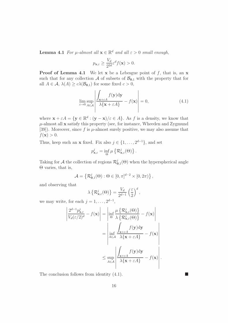
Lemma 4.1 For µ-almost all x ∈ Rd and all ε > 0 small enough,

px,ε ≥Vd

22dεdf(x) > 0.

Proof of Lemma 4.1 We let x be a Lebesgue point of f , that is, an xsuch that for any collection A of subsets of B0,1 with the property that forall A ∈ A, λ(A) ≥ cλ(B0,1) for some fixed c > 0,

limε→0

supA∈A

∣

∣

∣

∣

∣

∣

∣

∣

∫

x+εA

f(y)dy

λ{x+ εA}− f(x)

∣

∣

∣

∣

∣

∣

∣

∣

= 0, (4.1)

where x + εA = {y ∈ Rd : (y − x)/ε ∈ A}. As f is a density, we know that

µ-almost all x satisfy this property (see, for instance, Wheeden and Zygmund[39]). Moreover, since f is µ-almost surely positive, we may also assume thatf(x) > 0.

Thus, keep such an x fixed. Fix also j ∈ {1, . . . , 2d−1}, and set

pjx,ε = infΘ

µ{

Rjx,ε(Θ)

}

.

Taking for A the collection of regions Rj0,1(Θ) when the hyperspherical angle

Θ varies, that is,

A ={

Rj0,1(Θ) : Θ ∈ [0, π]d−2 × [0, 2π)

}

,

and observing that

λ{

Rjx,ε(Θ)

}

=Vd

2d−1

(ε

2

)d

,

we may write, for each j = 1, . . . , 2d−1,∣

∣

∣

∣

∣

2d−1pjx,εVd(ε/2)d

− f(x)

∣

∣

∣

∣

∣

=

∣

∣

∣

∣

∣

infΘ

µ{

Rjx,ε(Θ)

}

λ{

Rjx,ε(Θ)

} − f(x)

∣

∣

∣

∣

∣

=

∣

∣

∣

∣

∣

∣

∣

∣

infA∈A

∫

x+εA

f(y)dy

λ{x+ εA}− f(x)

∣

∣

∣

∣

∣

∣

∣

∣

≤ supA∈A

∣

∣

∣

∣

∣

∣

∣

∣

∫

x+εA

f(y)dy

λ{x+ εA}− f(x)

∣

∣

∣

∣

∣

∣

∣

∣

.

The conclusion follows from identity (4.1). �

16

Lemma 4.2 Fix x ∈ Rd, ε > 0 and Θ ∈ [0, π]d−2×[0, 2π). Let Nx,ε(Θ) be the

number of hyperplanes passing through d out of the observations X1, . . . ,Xn

and cutting the segment Sx,ε(Θ). Then, with probability 1,

Nx,ε(Θ) ≥N1

x,ε(Θ) . . .N2d−1

x,ε (Θ)

n2d−1−d.

Proof of Lemma 4.2 If one of the N jx,ε(Θ) (j = 1, . . . , 2d−1) is zero, then

the result is trivial. Thus, in the rest of the proof, we suppose that eachN j

x,ε(Θ) is positive and note that this implies n ≥ 2d−1.

Pick sequentially 2d−1 observations, say Xi1, . . . ,Xi2d−1

, in the 2d−1 regions

R1x,ε(Θ), . . . ,R2d−1

x,ε (Θ). By construction, the polytope defined by these 2d−1

points cuts the axis Lx,ε(Θ). Consequently, with probability 1, any hyper-plane drawn according to d out of these 2d−1 points cuts the segment Sx,ε(Θ).

The result follows by observing that there are exactly N1x,ε(Θ) . . .N2d−1

x,ε (Θ)such polytopes. �

Lemma 4.3 For 1 ≤ i1 < . . . < id ≤ n, let H(Xi1, . . . ,Xid) be the hyper-

plane passing through d out of the observations X1, . . . ,Xn. Then, for all

x ∈ Rd,

P {H(Xi1 , . . . ,Xid) ∩ Bx,δ 6= ∅} → 0 as δ ↓ 0.

Proof of Lemma 4.3 Given two hyperplanes H and H′ in Rd, we denote

by Φ(H,H′) the (dihedral) angle between H and H′. Recall that Φ(H,H′) ∈[0, π] and that it is defined as the angle between the corresponding normalvectors.

Fix 1 ≤ i1 < . . . < id ≤ n. Let Eδ be the event

Eδ ={

‖Xij − x‖ > δ : j = 1, . . . , d− 1}

,

and let H(x,Xi1 , . . . ,Xid−1) be the hyperplane passing through x and the

d−1 pointsXi1, . . . ,Xid−1. Clearly, on Eδ, the event {H(Xi1 , . . . ,Xid)∩Bx,δ 6=

∅} is the same as{

Φ(

H(x,Xi1, . . . ,Xid−1),H(Xi1, . . . ,Xid)

)

≤ Φδ

}

,

where Φδ is the angle formed by H(x,Xi1, . . . ,Xid−1) and the hyperplane

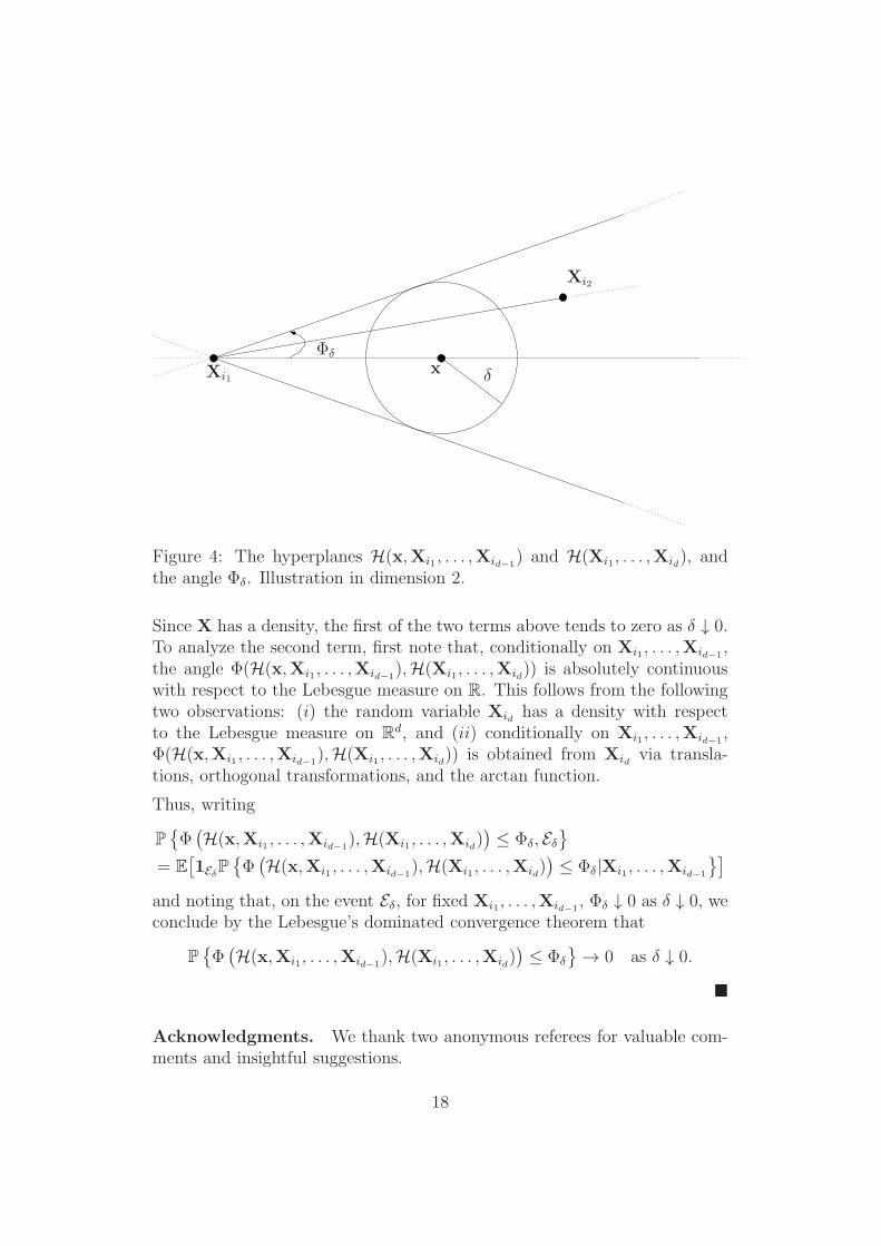
going trough Xi1, . . . ,Xid−1and tangent to Bx,δ (see Figure 4 for an example

in dimension 2).

Thus, with this notation, we may write

P {H(Xi1 , . . . ,Xid) ∩ Bx,δ 6= ∅}

≤ P{E cδ}+ P {H(Xi1 , . . . ,Xid) ∩ Bx,δ 6= ∅, Eδ}

≤ P{E cδ}+ P

{

Φ(

H(x,Xi1 , . . . ,Xid−1),H(Xi1, . . . ,Xid)

)

≤ Φδ, Eδ}

.

17

Xi1

Xi2

δxΦδ

Figure 4: The hyperplanes H(x,Xi1 , . . . ,Xid−1) and H(Xi1, . . . ,Xid), and

the angle Φδ. Illustration in dimension 2.

Since X has a density, the first of the two terms above tends to zero as δ ↓ 0.To analyze the second term, first note that, conditionally on Xi1, . . . ,Xid−1

,the angle Φ(H(x,Xi1 , . . . ,Xid−1

),H(Xi1, . . . ,Xid)) is absolutely continuouswith respect to the Lebesgue measure on R. This follows from the followingtwo observations: (i) the random variable Xid has a density with respectto the Lebesgue measure on R

d, and (ii) conditionally on Xi1, . . . ,Xid−1,

Φ(H(x,Xi1 , . . . ,Xid−1),H(Xi1, . . . ,Xid)) is obtained from Xid via transla-

tions, orthogonal transformations, and the arctan function.

Thus, writing

P{

Φ(

H(x,Xi1 , . . . ,Xid−1),H(Xi1, . . . ,Xid)

)

≤ Φδ, Eδ}

= E[

1EδP{

Φ(

H(x,Xi1 , . . . ,Xid−1),H(Xi1, . . . ,Xid)

)

≤ Φδ|Xi1, . . . ,Xid−1

}]

and noting that, on the event Eδ, for fixed Xi1, . . . ,Xid−1, Φδ ↓ 0 as δ ↓ 0, we

conclude by the Lebesgue’s dominated convergence theorem that

P{

Φ(

H(x,Xi1, . . . ,Xid−1),H(Xi1, . . . ,Xid)

)

≤ Φδ

}

→ 0 as δ ↓ 0.

�

Acknowledgments. We thank two anonymous referees for valuable com-ments and insightful suggestions.

18

References

[1] T. Anderson. Some nonparametric multivariate procedures based onstatistically equivalent blocks. In P. Krishnaiah, editor, Multivariate

Analysis, pages 5–27, New York, 1966. Academic Press.

[2] G. Biau and L. Devroye. On the layered nearest neighbour estimate,the bagged nearest neighbour estimate and the random forest method inregression and classification. Journal of Multivariate Analysis, 101:2499–2518, 2010.

[3] B. Chakraborty, P. Chaudhuri, and H. Oja. Operating transformationretransformation on spatial median and angle test. Statistica Sinica,8:767–784, 1998.

[4] B. Chazelle. Cutting hyperplanes for divide-and-conquer. Discrete Com-

putational Geometry, 9:145–158, 1993.

[5] T.M. Cover. Estimation by the nearest neighbor rule. IEEE Transac-

tions on Information Theory, 14:50–55, 1968.

[6] T.M. Cover. Rates of convergence for nearest neighbor procedures.In Proceedings of the Hawaii International Conference on Systems Sci-

ences, pages 413–415, Honolulu, 1968.

[7] T.M. Cover and P.E. Hart. Nearest neighbor pattern classification. IEEETransactions on Information Theory, 13:21–27, 1967.

[8] L. Devroye. A universal k-nearest neighbor procedure in discrimina-tion. In B.V. Dasarathy, editor, Nearest Neighbor Pattern Classification

Techniques, pages 101–106, Los Alamos, 1991. IEEE Computer SocietyPress.

[9] L. Devroye, L. Gyorfi, and G. Lugosi. A Probabilistic Theory of Pattern

Recognition. Springer-Verlag, New York, 1996.

[10] L. Devroye and A. Krzyzak. New multivariate product density estima-tors. Journal of Multivariate Analysis, 82:88–110, 2002.

[11] E. Fix and J.L. Hodges. Discriminatory analysis. Nonparametric dis-

crimination: Consistency properties. Technical Report 4, Project Num-ber 21-49-004, USAF School of Aviation Medicine, Randolph Field,Texas, 1951.

19

[12] E. Fix and J.L. Hodges. Discriminatory analysis: Small sample perfor-

mance. Technical Report 11, Project Number 21-49-004, USAF Schoolof Aviation Medicine, Randolph Field, Texas, 1952.

[13] M. Gessaman. A consistent nonparametric multivariate density estima-tor based on statistically equivalent blocks. The Annals of Mathematical

Statistics, 41:1344–1346, 1970.

[14] M. Gessaman and P. Gessaman. A comparison of some multivariate dis-crimination procedures. Journal of the American Statistical Association,67:468–472, 1972.

[15] L. Gordon and R.A. Olshen. Asymptotically efficient solutions to theclassification problem. The Annals of Statistics, 6:515–533, 1978.

[16] L. Gordon and R.A. Olshen. Consistent nonparametric regressionfrom recursive partitioning schemes. Journal of Multivariate Analysis,10:611–627, 1980.

[17] L. Gyorfi, M. Kohler, A. Krzyzak, and H. Walk. A Distribution-Free

Theory of Nonparametric Regression. Springer-Verlag, New York, 2002.

[18] M. Hallin and D. Paindaveine. Optimal tests for multivariate locationbased on interdirections and pseudo-Mahalanobis ranks. The Annals of

Statistics, 30:1103–1133, 2002.

[19] T.P. Hettmansperger, J. Mottonen, and H. Oja. The geometry of theaffine invariant multivariate sign and rank methods. Journal of Non-

parametric Statistics, 11:271–285, 1998.

[20] T.P. Hettmansperger and R.H. Randles. A practical affine equivariantmultivariate median. Biometrika, 89:851–860, 2002.

[21] W. Hoeffding. Probability inequalities for sums of bounded randomvariables. Journal of the American Statistical Association, 58:13–30,1963.

[22] J. Marcinkiewicz and A. Zygmund. Sur les fonctions independantes.Fundamenta Mathematicae, 29:60–90, 1937.

[23] C. McDiarmid. On the method of bounded differences. In J. Siemons,editor, Surveys in Combinatorics, 1989, London Mathematical SocietyLecture Note Series 141, pages 148–188. Cambridge University Press,1989.

20

[24] S. Meiser. Point location in arrangements of hyperplanes. Information

and Computation, 106:286–303, 1993.

[25] K.S. Miller. Multidimensional Gaussian Distributions. Wiley, New York,1964.

[26] H. Oja. Affine invariant multivariate sign and rank tests and correspond-ing estimates: A review. Scandinavian Journal of Statistics, 26:319–343,1999.

[27] H. Oja and D. Paindaveine. Optimal signed-rank tests based on hy-perplanes. Journal of Statistical Planning and Inference, 135:300–323,2005.

[28] E. Ollila, T.P. Hettmansperger, and H. Oja. Estimates of regressioncoefficients based on sign covariance matrix. Journal of the Royal Sta-

tistical Society Series B, 64:447–466, 2002.

[29] E. Ollila, H. Oja, and V. Koivunen. Estimates of regression coefficientsbased on lift rank covariance matrix. Journal of the American Statistical

Association, 98:90–98, 2003.

[30] R. Olshen. Comments on a paper by C.J. Stone. The Annals of Statis-

tics, 5:632–633, 1977.

[31] D. Paindaveine and G. Van Bever. Nonparametric consistent depth-based

classifiers. ECARES working paper 2012-014, Brussels, 2012.

[32] K.R. Parthasarathy. Probability Measures on Metric Spaces. AMSChelsea Publishing, Providence, 2005.

[33] V.V. Petrov. Sums of Independent Random Variables. Springer-Verlag,Berlin, 1975.

[34] C. Quesenberry and M. Gessaman. Nonparametric discrimination usingtolerance regions. The Annals of Mathematical Statistics, 39:664–673,1968.

[35] R.H. Randles. A distribution-free multivariate sign test based on interdi-rections. Journal of the American Statistical Association, 84:1045–1050,1989.

[36] M. Samanta. A note on uniform strong convergence of bivariate den-sity estimates. Zeitschrift fur Wahrscheinlichkeitstheorie und verwandte

Gebiete, 28:85–88, 1974.

21

[37] C.J. Stone. Consistent nonparametric regression. The Annals of Statis-

tics, 5:595–645, 1977.

[38] D.E. Tyler. A distribution-free M-estimator of multivariate scatter. TheAnnals of Statistics, 15:234–251, 1987.

[39] R.L. Wheeden and A. Zygmund. Measure and Integral. An Introduction

to Real Analysis. Marcel Dekker, New York, 1977.

22