An air quality balance index estimating the total amountof air pollutants at ground level

Paolo Trivero & Walter Biamino & Maria Borasi &Marco Cavagnero & Maya Musa &

Caterina Rinaudo & Veronica Sesia

Received: 12 January 2011 /Accepted: 27 July 2011 /Published online: 10 August 2011# Springer Science+Business Media B.V. 2011

Abstract A new index named Air Quality BalanceIndex (AQBI), which is able to characterise the amount ofpollution level in a selected area, is proposed. This indexis a function of the ratios between pollutant concentrationvalues and their standards; it aims at identifying allsituations in which there is a possible environmental riskeven when several pollutants are below their limit valuesbut air quality is reduced. AQBI is evaluated by using ahigh-resolution three-dimensional dispersion model: theair concentration for each substance is computed startingfrom detailed emissions sources: point, line and areaemissions hourly modulated. This model is driven withaccurate meteorological data from ground stations andremote sensing systems providing vertical profiles oftemperature andwind; these data are integrated with windand temperature profiles at higher altitudes obtained by aLocal Area Model. The outputs of the dispersion modelare compared with pollutant concentrations provided bymeasuring stations, in order to recalibrate emission data.A three-dimensional high resolution grid of AQBI data isevaluated for an industrial area close to Alessandria(Northern Italy), assessing air quality and environmentalconditions. Performance of AQBI is compared with the

Air Quality Index (AQI) developed by the U.S. Environ-mental Protection Agency. AQBI, computed taking intoaccount all pollutants, is able to point out situations notevidenced by AQI, based on a preset limited number ofsubstances; therefore, AQBI is a good tool for evaluatingthe air quality either in urban and in industrial areas. TheAQBI values at ground level, in selected points, are inagreement with in situ observations.

Keywords Air quality index . Air pollution . Pollutiondispersion model . Environmental monitoring

Introduction

At present, public opinion is often concerned about“quality of life”, which is strictly related to environ-mental issues. However, environmental decision-makers often rely on general observations and expertsuggestions; in some cases, especially after disasters,decisions are driven by public opinion or evenemotions (Esty 2002). Sometimes, a quantitativeevaluation is available but limited to specified casestudies (Esty et al. 2005). In order to provide aquantitative assessment, several indices have beendefined, based on direct observations of naturalphenomena; frequently, a number of parameters, notonly pollutants, can be taken into account in order todefine indices that are more comprehensive andtailored for specific situations (Singh and Hiremath2010; Žujić et al. 2009).

Environ Monit Assess (2012) 184:4461–4472DOI 10.1007/s10661-011-2278-1

P. Trivero (*) :W. Biamino :M. Borasi :M. Cavagnero :M. Musa :C. Rinaudo :V. SesiaDipartimento di Scienze dell’Ambiente e della Vita,Università del Piemonte Orientale “Amedeo Avogadro”,Viale Teresa Michel 11,15121 Alessandria, Italye-mail: paolo.trivero@mfn.unipmn.it

Dealing with air quality, a wide range of pollutantsshould be considered, produced by a huge range ofdifferent sources; however, a simplified approachcould be comprehensive and easier to manage.

In 1976, the United States Environment ProtectionAgency (USEPA) developed the Pollutant StandardsIndex (PSI), taking into account the concentrations offive pollutant substances (ozone, PM10, NO2, CO,SO2) (USEPA 1976). In 2000, this index was renamedthe Air Quality Index (AQI) after minor revisions,such as new standard values and the adding of PM2.5as reference pollutant.

For every pollutant, a set of reference levels(breakpoints, listed in Table 1) is defined and foreach pollutant P the following index IP is computed:

IP ¼ IHi � ILoBPHi � BPLo

ðCP � BPLoÞ þ ILo ð1Þ

where CP is the rounded concentration of pollutant P,BPHi is the breakpoint that is greater than or equal toCP, BPLo is the breakpoint that is less than or equal toCP, IHi is the AQI value corresponding to BPHi andILo is the AQI value corresponding to BPLo.

Among the six calculated indexes, the highestrepresents the AQI, reported as a value between zeroand 500, associated to a descriptive word (e.g.,"unhealthy") (USEPA 2006).

The AQI is officially used for air quality reports inUSA. Similar approaches are followed in othercountries with different names: RAQI (Revised AirQuality Index) in Taiwan (Cheng et al. 2004), ATMOindex in France, API index in the United Kingdom.

These approaches suffer from the followingshortcomings:

– A limited preset number of pollutants is considered.– Among the pollutants, only one is used to

compute AQI.– The index, based on in situ measures, is unable to

describe the situation of the areas far frommeasuring points.

In order to overcome these limitations, we suggest anew index named AQBI, which characterises theamount of pollution level in an area. The AQBI iscomputed as a function of ratios between concentrationvalues of all emitted pollutants and their standards. Ouraim is to characterize an area by starting from a detailedknowledge of pollutants sources and meteorological

conditions, using the most up-to-date models to com-pute pollutant dispersion and evaluate a synthetic indexfor every point of a regular spatial grid (resolution:250 m) in a defined area; the final result is a map of “airquality” values.

In different areas, emissions can be produced bydifferent types of sources. In industrial areas pollu-tants are mainly emitted from chimneys considered as“point sources”.

In urban areas, traffic can be considered the mainsource of air pollution (Kim and Guldmann 2011); inmany towns the high concentration of traffic airpollution is strictly correlated to the sanitary risk forurban population (Peng et al. 2009; Rioux et al.2010). Roads are considered as “line sources” andanalyzed with the support of a specially designedsoftware, able to process traffic data, to evaluatequality and amount of pollutants emitted by everyroad section.

There are situations with a great number ofwidespread sources in a well defined area; this is thecase of domestic heating or urban traffic, where it isalmost impossible to have precise data of every singlechimney or secondary road section. In this case, thewhole area is considered as an “area source” andemission figures are taken from statistically archiveddata, usually from inventories.

In the following paragraphs, AQBI is describedand the rationale behind the formula is explained.After a description of the utilized models, a case studyis presented and the results are discussed.

AQBI definition

Air pollution is a complex phenomenon involving anumber of related causes each one contributing withdifferent substances. Epidemiological studies on largepopulations have been unable to identify a thresholdconcentration below which ambient pollutants haveno effect on health. It is likely that within any largehuman population, there is such a wide range insusceptibility that some subjects are at risk even at thelowest end of the concentration range (World HealthOrganization 2003).

Emissions of many different types of pollutantscan lead to air and soil contamination producingstress for vegetation and animals, as well as to aworse quality of life with consequences on human

4462 Environ Monit Assess (2012) 184:4461–4472

health. A comprehensive air quality evaluation musttherefore be based on all emitted pollutants and not onlyon some reference substances. The concentrations ofvarious pollutants, in some cases below and in othercases above the limits imposed by law, contributed onthe whole to reduce the air quality.

With the aim of taking into account theprevious considerations we define an index, AQBI,which considers every substance compared with itslimit value:

AQBI ¼Y

i

e13

xix0i

� �2

ð2Þ

where xi represents the concentration values ofdifferent pollutants and x0i denotes the limit values.

The index varies between 0 and 1, where 1 meansno pollution and lower values correspond to a worseair quality. The use of a product function ofexponential terms let AQBI able to take into accountall pollutants influencing the air quality; everyexponential term, representing a specific pollutant,reduces the index value as a function of concentrationand can be considered as the coefficient of the nextterm. In this way, AQBI is suitable to describe everyenvironmental situation and it is possible to comparethe pollution level in different areas.

AQBI index is computed using the output of athree-dimensional model chain ending with theSPRAY Lagrangian model; the model has to beinitialized with pollutant concentrations emitted byeach source modulated in time and properly calibratedwith the data from air pollution control stations. Adiagnostic meteorological model, able to assimilatesurface measurements and vertical profiles of windand temperature, is applied in order to elaborate themeteorological three-dimensional fields of atmosphericparameters.

Dispersion model

In order to evaluate pollutant concentrations in lowertroposphere, we used the three-dimensional dispersionmodel SPRAY 3.0, a Lagrangian model that simulatesthe transport, dispersion and deposition of pollutantsemitted by sources of different kinds over complexterrain (Tinarelli et al. 2000; Gariazzo et al. 2007).The model can take into account complex situations,such as the presence of breeze cycles, strongmeteorological anomalies, low wind calm conditionsand recirculation zones (Gariazzo et al. 2004).Simulations can cover an area ranging from verylocal (less than one kilometre) to regional (hundreds

Table 1 List of breakpoints used for AQI evaluation

This Breakpoint Equal this AQI And this category

O3 (ppm) 8 h O3 (ppm) 1 ha PM10

(μg/m3)PM2.5

(μg/m3)CO (ppm) SO2 (ppm) NO2 (ppm) AQI

0.000–0.059 – 0–54 0.0–15.4 0.0–4.4 0.000–0.034 b 0–50 Good

0.060–0.075 – 55–154 15.5–40.4 4.5–9.4 0.035–0.144 b 51–100 Moderate

0.076–0.095 0.125–0.164 155–254 40.5–65.4 9.5–12.4 0.145–0.224 b 101–150 Unhealthy forsensitive groups

0.096–0.115 0.165–0.204 255–354 65.5–150.4 12.5–15.4 0.225–0.304 b 151–200 Unhealthy

0.116–0.374(0.155–0.404)c

0.205–0.404 355–425 150.5–250.4 15.5–30.4 0.305–0.604 0.65–1.24 201–300 Very unhealthy

d 0.405–0.504 425–504 250.5–350.4 30.5–40.4 0.605–0.804 1.25–1.64 301–400 Hazardousd 0.505–0.604 505–604 350.5–500.4 40.5–50.4 0.805–1.004 1.65–2.04 401–500 Hazardous

a Areas are required to report the AQI based on 8-h ozone values. However, there are areas where an AQI based on 1-h ozone valueswould be more protective. In these cases, the index for both the 8-h and 1-h ozone values may be calculated and the maximum AQIreportedb NO2 has no short-term standard and can generate an AQI only above a value of 200c The numbers in parentheses are associated 1-h values to be used in this overlapping category only (http://www.epa.gov/airnow)d Eight-hour O3 values do not define higher AQI values (≥301). AQI values of 301 or higher are calculated with 1-h O3 concentrations

Environ Monit Assess (2012) 184:4461–4472 4463

of kilometres) scales. The model has been validated inurban areas (Trini Castelli et al. 2003; Calori et al.2006); we used a high resolution grid in order toimprove the model performances for the traffic.

SPRAY outputs include, for each point of thecalculation grid, the spatial coordinates and the valuesof the predicted concentration for each pollutantconsidered during the simulation period.

In order to produce reliable results, SPRAYrequires a detailed description of pollutant sources,together with orography of the considered area andthree-dimensional fields of meteorological parame-ters. Some of these data are directly ingested by themodel, while other information needs to be pre-processed by ancillary software codes.

Traffic data pre-processing

Available data are expressed as traffic volumes:number of vehicles per kilometre, divided in differentspeed classes and vehicle classification; a procedure istherefore needed in order to evaluate emissions and toobtain a suitable input for SPRAY. TREFIC (TrafficEmission Factor Improved Calculation) 4.7 is thesoftware we used to estimate air pollution emissionsrelated to road traffic.

TREFIC is based on the COPERT III Europeanofficial methodology (Ntziachristos and Samaras2000), integrated and updated; it needs, as input data,the road net layout (from a GIS) and associated datafor each traffic situation (road type, number of lanes,steepness, average speed, number of vehicles for eachmacro class). Time modulations (traffic volumes,vehicle speed, and air temperature) can also bemanaged on an hourly, daily and monthly scale. Thevehicle fleet composition, for each type of road, isalso required since different vehicle categories areresponsible for different kinds of pollution.

TREFIC outputs the pollutant emissions for eachroad leg: CO, NOx, SO2, hydrocarbons (e.g., benzene),particulates (TSP, PM10, PM2.5), heavy metals (Pb,Cd, Fe, etc.), PAH (e.g., benzo-a-pyrene) on an hourlybasis or aggregated (yearly). Weighted average emis-sion factors for local vehicle fleets are also available.

Meteorological data

Lagrangian models require a three dimensional descrip-tion of meteorological fields in order to evaluate a three-

dimensional grid of the pollution concentrations.Ground level measurements need to be integrated withvertical profiles, acquired in different ways, for examplewith radiosondes or tethered balloons; there are howevera number of cost and air safety issues, limiting thepossibility of frequent and spatially closemeasurements.A significant contribution comes from ground-basedremote sensing: instruments such as RASS (RadioAcoustic Sounding System) and SODAR (SoundDetection and Ranging) are able to measure profiles,within the first hundreds of meters, with precision ofsome tenth of a degree for the temperature, 1.5° for winddirection, 0.3 m/s for wind intensity and about 10 m foraltitude.

RASS measures air vertical temperature profile inreal time with continuity, operating with acoustic andelectromagnetic waves. A Doppler radar measures thespeed, which depends on the local air temperature, ofan acoustic wave train sent towards the zenith.

SODAR measures wind profiles by emitting soundpulses and evaluating the frequency and amplitude ofthe atmospheric echoes during the time, beingacoustic waves backscattered by temperature inhomo-geneities in the air. Hourly temperature and windvalues, coming from ground measurement stations,and profiles obtained with RASS and SODAR as wellas the outputs of a meteorological LAM (LimitedArea Model) are assimilated by means of thediagnostic model MINERVE to be used into SPRAY.

The case study

The proposed methodology has been tested on theFraschetta area located inside the Municipality ofAlessandria (North-Western Italy), with a populationof about 16,000 and a surface area of about 90 km2

(Fig. 1). This area is characterized by the typicalconditions of Po Valley: atmospheric stability (thermalinversion at night) and low wind speed, which tendsto increase the pollution concentrations.

Since 1900, diversified industrial activities hadbegun to develop in this area. In particular there is anindustrial complex of around 1 km2 which includesproductive activities almost integrally tied up tofluorinated products, chemistry and organic perox-ides. During the past few decades, these activitieshave brought about contamination of the grounds. Atclose distance, another industrial area hosts a tyre

4464 Environ Monit Assess (2012) 184:4461–4472

factory and other numerous manufacturing industries.There is also a waste treatment plant, with a nowclosed landfill which has caused problems of ground-water contamination, biogas leaks in the adjacentsubsoil and emission of bad smelling odours (Zorzi etal. 2005). A motorway crosses the area, together withtwo national roads with a heavy traffic level, due bothto freight transport and commuters.

SPRAY model has been used to simulate thedispersion of pollutants emitted by all kinds of sources(point, area and line) located within the Fraschetta area.

In Fig. 1, the emission sources are represented:emission points with indication of pollutants emitted,motorway, national roads, main industrial areas andvillages.

The calculation domain is a square area of 144 km2

extending from 471,250 to 483,250 m UTM X andfrom 4,966,000 to 4,978,000 m UTMY (zone 32 N).The grid resolution is 250 m.

In order to describe the situation with high detail, wesimulated pollutant dispersion on a single uninterruptedepisode lasting 96 h, with 1-h time resolution. The

Fig. 1 Image of the study area. Point emissions (capital whiteletters): PM10 (A), CO (B), SOx (C), VOC (D), NOx (E), HF(F) and HCl (G). Motorway (orange line), national roads (red

lines), main industrial areas (blue) and villages (green). Weatherand remote sensing stations (yellow). Measurement stationsMS1 and MS2 managed by ARPA (white)

Environ Monit Assess (2012) 184:4461–4472 4465

simulation period has been selected in coincidence witha monitoring campaign carried out from 19 to 22September 2005 in Fraschetta area, in the frameworkof the EU funded LINFA Project (Life INtervention forFraschetta Area). During this campaign a great deal ofchemical and biological data were collected.

Point emissions

Point emissions, due to individual stacks, are distin-guished based on the characteristics of the stack (height,diameter), the plume (volume, temperature, exit velocity),the type and concentration of pollutant emitted.

Data are extracted from authorizations for airemission inventory of the municipality of Alessandria.The model input consists of 66 point sources, emittingthe following pollutants (indicated by capital letters):PM10 (A), CO (B), SO2 (C),VOC (D), NOx (E), HF (F)and HCl (G). Table 2 summarizes the total emission(expressed in kg/h) of each pollutant in the area ofsimulation due to the point sources taken into account.

In order to minimize SPRAY computation time,some minor point sources with negligible effect havebeen discarded (e.g., a pollutant emitted by a singlesource, for a limited time during the day).

Line emissions

Line emissions are due to the main roads crossing thearea of interest: the motorway (orange line in Fig. 1)and the national roads (red lines in Fig. 1).

The emission contribution due to traffic is deter-mined by means of TREFIC software that takes intoaccount the different kind of road (motorway, ruraland urban roads), the volume and the traffic speed.

Motorway traffic data come from the AISCAT(Italian association of motorways managers) database.National road network data were collected by theProvincial Council of Alessandria during a monitoringcampaign of the vehicle flow. During the monitoring

period, the road network was provided with inductionloop detectors for sensing, on an hourly basis, thepresence, speed and length of vehicles in both directionsof travel. The average composition of vehicle fleet forthe Province of Alessandria has been obtained by theItalian Automobile Association and used to define thepercentage of motorcycles compared with the vehicles.The collected information was used to create a databasecontaining the hourly transits for four macro categories:passenger cars, light duty vehicles, heavy duty vehicles,and motorcycles. The vehicle fleet has been also dividedinto the different COPERT categories, from “Pre Euro”to the most recent “Euro 4”.

The road graph was defined by identifying four mainaxes: the three legs of national roads and one leg ofmotorway. Every leg is described as a polyline with notraffic variations along space. Hourly modulation showsstrong variations among rush hours (high trafficvolumes) and nighttime, where the number of vehiclesis near to zero.

Area emissions

Since the simulation has been performed in autumnseason, during which domestic heating systems are stilloff, the main source of pollution in urban centres istraffic: in this case traffic is considered as an area source.Urban traffic emission is obtained by the regionalinventory INEMAR 2001; emission data have beenspatially disaggregated to a 250-m grid and temporallyextrapolated on an hourly modulation over the simula-tion period. Space disaggregation is necessary to allocateurban traffic emissions according to the distribution ofresidential areas within the municipality territory takinginto account the percentage of residential area containedin each cell of the grid; as regards time disaggregation,daily, weekly and annual time profiles were used, asobtained from observations of urban traffic.

The emission contribution due to the main roads,quoted in Section 4.2, has been excluded from thearea emissions.

AQBI evaluation

The SPRAY dispersion model has been used to evaluatethe contribution of each typology of source to theoverall air pollution, performing a separate simulation ofdispersion of pollutants emitted into the air.

Table 2 Total emission of each pollutant in the area by thepoint sources considered in the simulation area (kg/h) and theircode

Pollutant PM10 CO SO2 VOC NOx HF HCl

Emission (kg/h) 22.6 21.2 43.9 2.3 54.4 0.02 0.002

Code A B C D E F G

4466 Environ Monit Assess (2012) 184:4461–4472

Meteorological measurements facilities are availablein Fraschetta area. In Castelceriolo landfill, we have aremote sensing stationwith a RASS (Bonino and Trivero1985; Biamino et al. 2002) and a SODAR continuouslyacquiring vertical profiles of temperature and windvector, respectively. A weather station is located inLobbi, close to the remote sensing station (Fig. 1).

RASS and SODAR profiles are available startingfrom a minimum height, according to instrumentfeatures, 80 m for the RASS and 66 m for the SODAR.Temperature at ground level is supplied by a sensorlocated at the basis of the RASS and by the Lobbistation; while the anemometer in Lobbi measures windat the ground level.

Our RASS produces vertical thermal profilesreliable within an altitude of about 400–600 m. Inorder to have a comprehensive description of meteo-rological fields up to higher altitudes, an additionalinput is considered: temperature profiles taken fromdaily runs of CALMET-SMR meteorological model,managed by Regional Meteorological Service ofARPA (Regional Agency for Prevention and Envi-ronment) Emilia Romagna. This service, starting froma number of available data, produces meteorologicalprofiles over the whole of northern Italy within 5-kmhorizontal grids (Deserti et al. 2001).

The temperatures at ground level, acquired withsensors installed at the basis of the RASS and in Lobbistation, are averaged; this value of temperature and thefirst values measured by the RASS starting at thealtitude of 80 m are interpolated to fit a parabolicfunction. Conversely, the higher part of the thermalprofile is given by CALMET model; the upper value ofevery RASS sounding is linearly interpolated toCALMET value at 2,500 m. Fig. 2 shows an exampleof temperature RASS profile compared with theCALMET model profile: RASS data is reliable atlower levels but limited to the first hundreds of meters,although model data cannot accurately describe theground based thermal inversion, they offer a reliableevaluation at higher altitudes. The use of the abovedescribed interpolation procedure, instead of applyinga standard parameterization, allows a better evaluationof the thermodynamic atmospheric structure.

These profiles, together with the pollutant emissionvalues, are the input of the SPRAY model.

SPRAY model gives as output the hourly three-dimensional grids of pollutant concentrations. In orderto calculate the AQBI for each grid point at ground

level, according to Eq. 2, we added to these concen-trations a background, due to the sources of pollutionoutside the calculation domain. The background valuewas evaluated by a comparison between the officialmeasurements by the ARPA measuring stations (pointsMS1, MS2 in Fig. 1) and those evaluated by the modelin the same points. For typical emissions related toindustrial activities, we have compared the in situmeasured concentrations with those calculated by themodel and we have verified that they have differentvalues but the same concentration ratio; thereforeemission values have been calibrated on the basis ofmeasured concentration data. PM10, CO, SO2,VOC,NOx, NO2 HF and HCl concentrations values, togetherwith ozone as measured by ground stations, have beenincluded in AQBI evaluation.

In Eq. 2, we use the standards introduced by theEuropean directives (Table 3) (EU 1999; 2000; 2002).

AQBI map

AQBI values (ranging from 0 to 1) have been linearlydivided into seven intervals, with the same names andcolours of AQI scale: good (green), moderate (yellow),

0

500

1000

1500

2000

2500

0 5 10 15 20

Temperature (°C)A

ltit

ud

e (m

)

T model T RASS

Fig. 2 Example of RASS temperature profile connected toprofile from model. The purple line is an interpolation ofCALMET data (crosses)

Environ Monit Assess (2012) 184:4461–4472 4467

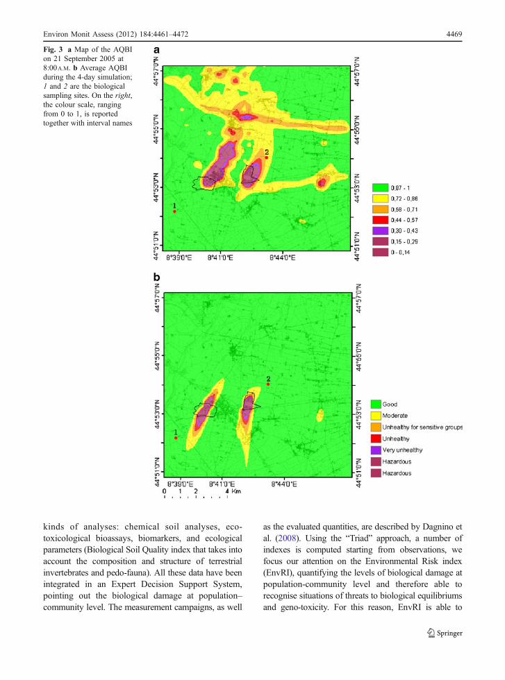
unhealthy for sensitive groups (orange), unhealthy (red),very unhealthy (purple), and hazardous (maroon—thelast two intervals), in order to visually compare AQBIand AQI. This scale is shown in Fig. 3.

The AQBI values have been calculated in a grid at250 m spatial resolution. Figure 3 shows the rastermaps obtained by interpolating AQBI values in thegrid points.

Figure 3a shows the AQBI calculated with theoutput of the model on 21 September 2005 at 8:00A.M. (the dominant wind direction was South-West),taken as a typical example of high level of pollution.

The maps show that the areas with the highest airpollution levels are in proximity of the two largerindustries, of the motorway and the national roads.

The time variability of AQBI values is strongly relatedto emissions time modulation, as well as to differentmeteorological conditions during the simulation period.Figure 3b shows the AQBI map index calculated withthe average concentration values during the 4-daysimulation; it is interesting to note that the roads appear“less hazardous” than factories; this is because majorpoint emissions are continuous during simulation time,while traffic pollution is concentrated in a few hours(typically in the morning and in the afternoon).

By computing AQBI with average values, it ispossible to evaluate the “mean situation”, that is, theexposition to pollutants of people living in the area; inthis case, the situation can be described as good–moderate almost everywhere, except for the area closeto factories.

The minimum, maximum, mean and standarddeviation values for each substance, measured in theMS2 point (Fig. 1) during the whole simulation, andtheir standards as defined by EU legislation, arereported in Table 3.

AQI and AQBI comparison

We have compared our index with the well-established AQI in order to assess the performanceof the two indices in the same situation on 21September 2005 at 8:00A.M. The AQI has beencalculated according to Eq. 1 with U.S. standardsand is represented in the map in Fig. 4a, to becompared with the map of our index (Fig. 3a).

AQBI, taking into account all kind of emissionincluding industrial ones like HF and HCl, anddepending on all pollutants, is able to highlight theoverall situation, in particular close to the industrialareas and along a stretch of motorway and thenational roads. The AQI value instead, being calcu-lated using less restrictive standards and only thehighest value among the five pollutants considered,reports two limited areas as polluted.

In order to carry out a better comparison, the AQBIhas been calculated for the same situation using USAstandards and taking into account only the five AQIpollutants. The resulting map is represented inFig. 4b. Even under these conditions AQBI is ableto highlight the presence of the motorway and thenational roads, but is unable to show the presence ofall industrial plants.

AQBI and EnvRi comparison

In the framework of LINFA project in 2006, biologicaland ecological state of Fraschetta area was subject to athorough survey: samples of soil, collected duringseasonal measurements campaigns in different sitesindicated with 1 and 2 in Figs. 3 and 4, were analysed.

A bio-monitoring programme has been carried out:the samples were characterized employing different

Min Max Mean SD Air concentration standards (μg/m³)

PM10 20 56 24 8 50

CO 700 1,000 832 71 10,000

SO2 2 9 4 1 350

VOC 4 69 15 17 200

NO 1 66 12 14 200

NO2 11 63 32 13 200

HF 0 154 13 30 20

HCl 0 526 44 103 50

O3 7 85 31 24 120

Table 3 Minimum,maximum, mean andstandard deviationconcentration values(μg/m3), over the 72 h in theMS2 point, and their EUstandards

4468 Environ Monit Assess (2012) 184:4461–4472

kinds of analyses: chemical soil analyses, eco-toxicological bioassays, biomarkers, and ecologicalparameters (Biological Soil Quality index that takes intoaccount the composition and structure of terrestrialinvertebrates and pedo-fauna). All these data have beenintegrated in an Expert Decision Support System,pointing out the biological damage at population–community level. The measurement campaigns, as well

as the evaluated quantities, are described by Dagnino etal. (2008). Using the “Triad” approach, a number ofindexes is computed starting from observations, wefocus our attention on the Environmental Risk index(EnvRI), quantifying the levels of biological damage atpopulation-community level and therefore able torecognise situations of threats to biological equilibriumsand geno-toxicity. For this reason, EnvRI is able to

Fig. 3 a Map of the AQBIon 21 September 2005 at8:00A.M. b Average AQBIduring the 4-day simulation;1 and 2 are the biologicalsampling sites. On the right,the colour scale, rangingfrom 0 to 1, is reportedtogether with interval names

Environ Monit Assess (2012) 184:4461–4472 4469

describe the effect of pollutants on animal and vegetallife

For comparison purposes, EnvRI index valueshave been taken into account, utilising the averagevalues between “Summer 2005” and “Fall 2005”obtained during measurement campaigns, because ourAQBI is evaluated based on data acquired across theseasonal change. EnvRI reached the value 0.32 at

point 1 and 0.38 at point 2, indicating a fairly goodsituation in both measurement points because thisindex may vary from 0 (no environmental risk at all)to 1 (heavy risk). The AQBI values, computed onmean pollutant concentrations, are 0.93 at point 1 and0.90 at point 2, confirming the fairly good situationand both indexes show that the point 1 is less pollutedthan the point 2.

Fig. 4 a Map of the AQIcalculated on 21 September2005 at 8:00A.M. b Map ofthe AQBI calculated on 21September 2005 at 8:00A.M.considering only PM10,CO, SO2, NO2 and O3 withU.S. standards

4470 Environ Monit Assess (2012) 184:4461–4472

Conclusions

A high-resolution three-dimensional dispersion modelhas been employed to determine the air concentrations ofpollutants at ground level considering emission sourcesin an industrial area. Afterwards, the global amount ofpollution has been summarized by introducing AQBI,which is function of the ratios between concentrationvalue of each pollutant and its limit value. The AQBImap, calculated on a polluted industrial area, represents amap of air quality.

The comparison between AQBI and AQI valuesproves the efficiency of our index in assessing thelevel of air pollution in industrial districts as well as inthe surrounding areas; situations, where many pollu-tants are present, even at low levels, are betterdescribed by AQBI than by AQI.

AQBI is able to describe the mean situation over amonitored area by averaging hourly AQBI maps overlong periods, and therefore can be also used as a toolto evaluate the anthropogenic activity effects or, forexample, to estimate the contribution of new roads orindustrial estates.

The pollutant dispersion is currently evaluated byusing wind and temperature fields measured orobtained by meteorological models. By integrating ameteorological forecasting model into the modelchain, AQBI could acquire forecasting abilities andoperate as an instrument for air quality management.Moreover, this kind of approach can potentially beutilised as a management tool for factories, with theaim to reduce emissions in critical situations such asstrong thermal inversions in order to mitigate theeffects of pollution emissions.

The main features of this approach are thepossibility to take into account all the pollutantspresent in the study area as well as the outputpresented as a map with very high spatial resolution,instead of values from single, uncorrelated, measure-ment points.

Acknowledgements This work was supported by “FondazioneCassa di Risparmio di Alessandria” in the framework of “Ricerca einnovazione per Alessandria” financing scheme—year 2008 andby European Commission in the framework of the EU-funded“LINFA” project (“LIFE—Environment Intervention for FraschettaArea”—Ref. LIFE04 ENV/IT/000442). Traffic data of provincialroad network have been supplied by the Provincial Council ofAlessandria.

References

Biamino, W., Bonino, G., Marcacci, P., Menegazzo, L.,Rossello, R., Trivero, P. (2002). An integrated RASS—SODAR system for PBL monitoring and pollutionforecast. Proc. of the 11th International Symposium onAcoustic Remote Sensing and Associate Techniques of theAtmosphere and Oceans, 24–28 June 2002, Rome, Italy,197–200.

Bonino, G., & Trivero, P. (1985). Automatic tuning of Braggcondition in a Radio-Acoustic System for PBL tempera-ture profile measurement. Atmospheric Environment, 19(6), 973–978.

Calori, G., Clemente, M., De Maria, R., Finardi, S., Lollobrigida,F., & Tinarelli, G. (2006). Air quality integrated modelling inTurin urban area. Environmental Modelling and Software, 21(4), 468–476.

Cheng, W. L., Kuo, Y. C., Lin, P. L., Chang, K. H., Chen, Y. S.,Lin, T. M., et al. (2004). Revised air quality index derivedfrom an entropy function. Atmospheric Environment, 38(3), 383–391.

Dagnino, A., Sforzini, S., Dondero, F., Fenoglio, S., Bona, E.,Jensen, J., et al. (2008). A “weight-of-evidence” approachfor the integration of environmental “triad” data to assessecological risk and biological vulnerability. IntegratedEnvironmental Assessment and Management, 4(3), 314–326.

Deserti, M., Savoia, E., Cacciamani, C., Golinelli, M.,Kerschbaumer, A., Leoncini, G., et al. (2001). Operationalmeteorological pre-processing at Emilia-Romagna ARPAMeteorological Service as a part of a decision supportsystem for Air Quality Management. International Journalof Environmental and Pollution, 16, 571–582.

Esty, D. C. (2002). Why measurement matters. I. In D. C. Esty& P. Cornelius (Eds.), Environmental performance mea-surement: The global 2001–2002 report. New York:Oxford University Press.

Esty, D. C., Levy, M., Srebotnjak, T., & de Sherbinin, A.(2005). Environmental sustainability index: Benchmarkingnational environmental stewardship. New Haven, CT: YaleCenter for Environmental Law & Policy.

European Union (1999). Council Directive 1999/30/EC of 22April 1999 relating to limit values for sulphur dioxide,nitrogen dioxide and oxides of nitrogen, particulate matterand lead in ambient air. http://eur-lex.europa.eu/LexUriServ/LexUriServ.do?uri=OJ:L:1999:163:0041:0060:EN:PDF.Accessed 11 November 2010.

European Union (2000). Directive 2000/69/EC of the EuropeanParliament and of the Council of 16November 2000 relating tolimit values for benzene and carbon monoxide in ambient air.http://eur-lex.europa.eu/LexUriServ/LexUriServ.do?uri=OJ:L:2000:313:0012:0021:EN:PDF. Accessed 11 November2010.

European Union (2002). Directive 2002/3/EC of the EuropeanParliament and of the Council of 12 February 2002 relating toozone in ambient air. http://eur-lex.europa.eu/LexUriServ/LexUriServ.do?uri=OJ:L:2002:067:0014:0030:EN:PDF.Accessed 11 November 2010.

Gariazzo, C., Pelliccioni, A., Bogliolo, M., & Scalisi, G.(2004). Evaluation of a Lagrangian Particle Model

Environ Monit Assess (2012) 184:4461–4472 4471

(SPRAY) to assess environmental impact of an industrialfacility in complex terrain.Water, Air, & Soil Pollution, 155(1), 137–158.

Gariazzo, C., Papaleo, V., Pelliccioni, A., Calori, G., Radice, P.,& Tinarelli, G. (2007). Application of a Lagrangianparticle model to assess the impact of harbour, industrialand urban activities on air quality in the Taranto area, Italy.Atmospheric Environment, 41(30), 6432–6444.

Kim, Y., & Guldmann, J. M. (2011). Impact of traffic flows andwind directions on air pollution concentrations in Seoul,Korea. Atmospheric Environment, 45, 2803–2810.

Ntziachristos, L., & Samaras, Z. (2000). COPERT III computerprogramme to calculate emissions from road transport—Methodology and Emission Factors (version 2.1). Techni-cal Report No 49. European Environmental Agency.

Peng, R. D., Dominici, F., & Welty, L. J. (2009). A Bayesianhierarchical distributed lag model for estimating the timecourse of risk of hospitalization associated with particulatematter air pollution. Journal of the Royal StatisticalSociety: Series C (Applied Statistics), 58(1), 3–24.

Rioux, C. L., Gute, D. M., Brugge, D., Peterson, S., &Parmenter, B. (2010). Characterizing urban traffic expo-sures using transportation planning tools: an illustratedmethodology for health researchers. Journal of UrbanHealth: Bulletin of the New York Academy of Medicine, 87(2). doi:10.1007/s11524-009-9419-7.

Singh, P. K., & Hiremath, B. N. (2010). Sustainable livelihoodsecurity index in a developing country: A tool fordevelopment planning. Ecological Indicators, 10, 442–451.

Tinarelli, G., Anfossi, D., Bider, M., Ferrero, E., & TriniCastelli, S. (2000). A new high performance version of theLagrangian particle dispersion model SPRAY, some casestudies. In S. E. Gryning & E. Batchvarova (Eds.), Airpollution modelling and its applications XIII (pp. 499–507). New York: Plenum Press.

Trini Castelli, S., Anfossi, D., & Ferrero, E. (2003). Evaluationof the environmental impact of two different heatingscenarios in urban area. International Journal of Environ-ment and Pollution, 20, 207–217.

[USEPA] US Environmental Protection Agency (1976). Guide-line for public reporting of daily air quality—PollutantStandards Index (PSI). Report no. EPA-450/2-76-013.

[USEPA] US Environmental Protection Agency (2006). Guide-lines for the Reporting of Daily Air Quality—the AirQuality Index (AQI). Report no. EPA-454/B-06-001.

World Health Organization (WHO) (2003). Health Aspects ofAir Pollution with Particulate Matter, Ozone and NitrogenDioxide.

Zorzi, M., Dagnino, A., Delucchi, F., Dondero, F., Borasi, M.,Cossa, G., Ariati, L., et al. (2005). Monitoring and riskassessment activities of exhausted rubbish dump character-ized by a release of leachate in the superficial groundwateraquifer. Proc. of the 10th International Waste Managementand Landfill Symposium. CISA, Environmental SanitaryEngineering Centre: S. Margherita di Pula, Cagliari, Italy.

Žujić, A. M., Radak, B. B., Filipović, A. J., & Marković, D. A.(2009). Extending the use of air quality indices to reflecteffective population exposure. Environmental Monitoringand Assessment, 156, 539–549.

4472 Environ Monit Assess (2012) 184:4461–4472