An Algorithm for Clustered Data Generalized Additive

JSS Journal of Statistical SoftwareAugust 2005, Volume 14, Issue 8. http://www.jstatsoft.org/

An Algorithm for Clustered Data Generalized

Additive Modelling with S-PLUS

Lin Yee HinPrivate Medical Practitioner

Vincent CareyHarvard Medical School

Abstract

We present a set of functions in S-PLUS to implement the clustered data generalizedadditive marginal modelling (CDGAM) strategy proposed by Berhane and Tibshirani(1998). A variety of working correlation structures are supported, and the regressionbasis may include components from the family of smoothing splines.

Keywords: generalized estimating equations, clustered data analysis.

1. Introduction – Notations and theoretical background

The CDGAM algorithm for the semi-parametric setting presented in this paper implementsfitting methods for a class of generalized additive models for clustered data with observations(yit,xit). Here t = 1, · · ·,mi indexes observation times within the ith cluster, i = 1, · · ·, n; yit

is the response with expected value µit and xit is a (p+ q)× 1 vector of covariates. There arep parameters to be estimated under a standard generalized linear modeling framework, andq smooth functional parameters to be estimated non-parametrically. The marginal mean ofthe response is related to the parameters and covariates by

g(µit) = ηit = β0 + β1Xit1 + · · ·+ βpXitp + f1(Xit(p+1)) + · · ·+ fq(Xit(p+q)) (1)

The marginal variance of the response,VAR(yit), depends functionally on the marginal meanthrough the function v(µ)it. Hence

ηit = ηtotal,it = ηparametric,it + ηnonparametric,it (2)

We refer to the 1 to (p+ 1) components of (1) as the parametric component and components(p+ 2) to (p+ q) as the nonparametric component of the model.Estimation proceeds by forming the adjusted dependent variable McCullagh and Nelder (1989)

z = η + D−1(y − µ) (3)

http://www.jstatsoft.org/

2 An Algorithm for Clustered Data Generalized Additive Modelling with S-PLUS

where D = D1 ⊕ D2 ⊕ · · · ⊕ Dn and using iterative reweighted least squares with weightsW = W1⊕W2⊕· · ·⊕Wn and Wi = DiV−1

i Di. Di is ami×mi diagonal matrix with diagonalelements being ∂µit/∂ηit. Vi is defined as Vi = (A1/2

i Ri(α)A1/2i )/φ, with Ai being the

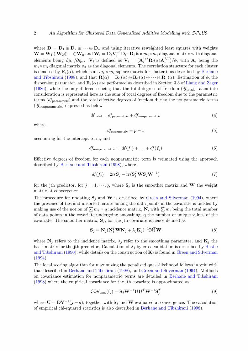
mi×mi diagonal matrix vit as the diagonal elements. The correlation structure for each clusteris denoted by Ri(α), which is an mi×mi square matrix for cluster i, as described by Berhaneand Tibshirani (1998), and that R(α) = R1(α)⊕R2(α)⊕ · · · ⊕Rn(α). Estimation of φ, thedispersion parameter, and Ri(α) are performed as described in Section 3.3 of Liang and Zeger(1986), while the only difference being that the total degrees of freedom (dftotal) taken intoconsideration is represented here as the sum of total degrees of freedom due to the parametricterms (dfparametric) and the total effective degrees of freedom due to the nonparametric terms(dfnonparametric) expressed as below

dftotal = dfparametric + dfnonparametric (4)

wheredfparametric = p+ 1 (5)

accounting for the intercept term, and

dfnonparametric = df(f1) + · · ·+ df(fq) (6)

Effective degrees of freedom for each nonparametric term is estimated using the approachdescribed by Berhane and Tibshirani (1998), where

df(fj) = 2trSj − tr(STj WSjW−1) (7)

for the jth predictor, for j = 1, · · · , q, where Sj is the smoother matrix and W the weightmatrix at convergence.

The procedure for updating Sj and W is described by Green and Silverman (1994), wherethe presence of ties and unsorted nature among the data points in the covariate is tackled bymaking use of the notion of

∑mi × q incidence matrix, N, with

∑mi being the total number

of data points in the covariate undergoing smoothing, q the number of unique values of thecovariate. The smoother matrix, Sj , for the jth covariate is hence defined as

Sj = Nj(NTj WNj + λjKj)−1NT

j W (8)

where Nj refers to the incidence matrix, λj refer to the smoothing parameter, and Kj thebasis matrix for the jth predictor. Calculation of λj by cross-validation is described by Hastieand Tibshirani (1990), while details on the construction of Kj is found in Green and Silverman(1994).

The local scoring algorithm for maximizing the penalized quasi-likelihood follows in vein withthat described in Berhane and Tibshirani (1998), and Green and Silverman (1994). Methodson covariance estimation for nonparametric terms are detailed in Berhane and Tibshirani(1998) where the empirical covariance for the jth covariate is approximated as

COVemp(fj) = SjW−1UUTW−1STj (9)

where U = DV−1(y−µ), together with Sj and W evaluated at convergence. The calculationof empirical chi-squared statistics is also described in Berhane and Tibshirani (1998).

Journal of Statistical Software 3

2. Implementation of CDGAM

The code discussed in this paper has been developed under S-PLUS 2000 Professional Release 1for Windows.

In addition to some auxiliary scripts, the library contains the following main functions:cdgam function to fit the CDGAMcdgam.par script called from cdgam to fit the parametric part

of the modelcdgam.nonpar script called from cdgam to fit the nonparametric part

of the modelsummary.cdgam function to display the summary results of model fitting

performed by cdgamplot.cdgam function to plot the estimated functional form against

the respective covariates

2.1. General schematics

The present cdgam implementation involves three major steps:

1. estimation of starting values for iterations in cdgam by fitting a generalized additivemodel under independent correlation structure as described by Hastie and Tibshirani(1990),

2. estimation of the correlation matrix for each cluster and fitting the parametric portionof cdgam using the framework of GEE,

3. estimation of the non-parametric portion of the cdgam.

In Step 1, a generalized additive model is being fitted under the independence (R(α)) frame-work, but not using the GEE sandwich method, in order to obtain fitted values for theparametric and nonparametric covariates to be used in Step 2. The script in S for performingStep 1 is gam(), an algorithm in S-PLUS that fits the generalized additive model when thedata points are not correlated. See Chambers and Hastie (1993) for operation details.

Calculations for Step 2 and Step 3 are coordinated by a script called cdgam(). Step 2 isexecuted by cdgam.par(). Step 3 is executed by cdgam.nonpar(). cdgam() separates thecovariates into two groups. Covariates requiring parametric estimation are passed, withincdgam(), to cdgam.par() where conventional GEE fitting is performed until local conver-gence is reached. Then, the results from cdgam.par() is passed into cdgam.nonpar() toperform the nonparametric estimation until local convergence criteria is reached. Finally,global convergence of the parametric and nonparametric covariates is checked.

The presence of local and global covergence arise from the nature of the iteration architecture.The outer loop is a local scoring procedure. In the inner loop, the Fisher scoring iteration isperformed in cdgam.par() while the Gauss-Seidel iteration is performed in cdgam.nonpar().Local convergence criteria refers to the convergence criteria used within either cdgam.par() orcdgam.nonpar(), while global convergence criteria refers to the criteria used within cdgam().

Local convergence within cdgam.par() is checked by measuring the values of absolute dif-ference between each of the estimated coefficients from the present Fisher scoring interation


(βnew) and the immediately preceeding iteration (βold), defined as ∆(βnew, βold). Parametriclocal convergence is considered reached when all values are smaller than a predeterminedvalue, called the local tolerance. In cdgam.par(), the local tolerance is set at 5× 10−4, andit can be adjusted by the user within cdgam.par(). Hence the parametric local convergencefor cdgam.par() is expressed as

∆(βnew, βold) = max(‖βnew − βold‖) (10)

Local convergence within cdgam.nonpar() is checked by measuring the fraction of absolutechange in the values of the estimated nonparametric functions between those estimated fromone Gauss-Seidel iteration (fnew) and the immediately preceeding iteration (fold), definedas ∆(fnew, fold). Nonparametric local convergence is considered reached when all values aresmaller than a predetermined value, called the local tolerance. In cdgam.nonpar(), the localtolerance is set at 0.02, and it can be adjusted by the user within this script. Hence thenonparametric local convergence is:

∆(fnew, fold) = max

{(‖fnew − fold‖

‖fold‖

}(11)

where, in the spirit of Equation (1), we can define fnew = f1,new + · · · + fq,new and fold =f1,old + · · ·+ fq,old respectively.

Global covergence within cdgam() is checked by measuring the fraction of absolute changein the values of the estimated nonparametric functions between those estimated from onelocal-scoring iteration (Fnew) and the immediately preceeding local-scoring iteration (Fold),defined as ∆(Fnew,Fold). Nonparametric global convergence is considered reached when allvalues are smaller than a predetermined value, called the global tolerance. Similar to thenonparametric local convergence criteria, the global tolerance in cdgam() is set at 5 × 10−5,and it can be adjusted by the user within cdgam(). It follows that

∆(Fnew,Fold) = max

{(‖Fnew − Fold‖

‖Fold‖

}(12)

where, we define Fnew = F1,new + · · ·+ Fq,new and Fold = F1,old + · · ·+ Fq,old respectively.

The cdgam() script makes use of the results of calculation performed by gam(· · ·,x=T) in orderto retrieve three entities: (1) data matrix for the nonparametric terms, (2) effective degree offreedom for each nonparametric term, and (3) estimated values for the nonparametric terms.

The data matrix for the nonparametric terms is used for calculation of the incidence matricesfor the jth nonparametric term, Nj . This, together with the estimation of smoothing pa-rameter λj and basis matrix Kj , are used to construct the smoother matrix Sj for the jthnonparametric covariate later on. For fast calculation, the calculation of λj is made based-on the S-PLUS built-in function called smooth.spline(). For a domain of unique x valuesx1, x2, · · · , xt on some interval [x1, xt], satisfying x1 < x2 < · · · < xt over which smoothing iscarried out, where x1 < x2 < · · · < xt, the spar value of the object fitted by smooth.spline()returns a value, denoted as ξ, that is connected to λj as below:

λj = ξ(xt − x1)3 (13)


The effective degrees of freedom and the estimated values for the nonparametric terms arethen passed, within cdgam(), into cdgam.par() where the correlation structure R(α),and thedispersion scale parameter φ are estimated. Then, using these two entities, the Fisher scoringiterations for estimating the parametric covariates is performed. At local convergence, testsfor significance as described in Liang and Zeger (1986) is carried out.The results of estimated values for the parametric covariates, R(α), and φ at convergence incdgam.par() are then used by cdgam.nonpar() to perform Gauss-Seidel iterations in orderto fit the nonparametric terms. At local convergence, the chi-squared test of significance asdescribed in Berhane and Tibshirani (1998) is carried out. Then, the updated effective degreeof freedom and estimated values for the nonparametric terms are passed into cdgam.par()again for the second local scoring iteration until global convergence is reached.

2.2. Handling of intracluster correlation structure

The calculation of within cluster correlation matrices Ri(α) is performed in the script calledcdgam.par() where the Pearson’s residual calculated using the most update ηparametric,it,ηnonparametric,it, dfparametric and dfnonparametric for each cluster. The options of correlationstructures currently supported are:

1. exchangeable correlation, otherwise known as uniform correlation model, where thereis a positive correlation coefficient, α, between any two measurements within the samecluster and that α is the same across all clusters;

2. stratified exchangeable correlation, where there is a positive correlation coefficient, αi,between any two measurements within the same cluster, and variation of αi acrossclusters is allowed;

3. first order autoregressive model for evenly spaced time scale; and

4. first order autoregressive model for unevenly spaced time scale. The methods appliedin this algorithm follows directly from that described in Liang and Zeger (1986).

Since R(α) = R1(α) ⊕ R2(α) ⊕ · · · ⊕ Rn(α) is a blocked-diagonal matrix, calculation ofR−1(α) required in the calculation of weights W makes use of the identity R−1(α) =R−1

1 (α) ⊕ R−12 (α) ⊕ · · · ⊕ R−1

n (α) in order to save computing memory and time. There-fore, two subroutines options need to be specified in cdgam(), where the one assigned tothe option called alpfun specifies one of the four options of correlation structures describedabove, and one to the option called wcorigen calculates R−1

i (α) for clusters i = 1, · · · n.In addition, there is an input option, called cor.met, in cdgam() that needs to be specifiedfor calculation of certain types of correlation structure specification. For uniform correlationstructure, it need not be specified. For stratified uniform correlation structure, the variableassigned to cor.met is the pointer variable identifying the cluster origin of the data points. Forfirst order autoregressive model for evenly spaced time scale, assignment to cor.met constitutesa matrix with two columns, the first is the pointer variable identifying the cluster origin ofthe data points, while the second is the recording of the times at which the correspondingdata points were observed.This arrangement leaves room for extensions by users where, by simply writing the scriptsfor alpfun and wcorigen, one can deploy the present cdgam to cater for other types ofintracluster correlation structures.


2.3. Choice of smoothing parameter

Leave-one-out generalized cross-validation is computationally intensive in the setting of gen-eralized semiparametric modelling, requiring re-computation of the entire iterative fit for eachvalue of λ on a grid in order to carry out the necessary minimization over λ (Green and Silver-man 1994), and its performance in practice is sometimes questionable (Hastie and Tibshirani1990).The use of empirical-bias bandwith selector (EBBS) (Ruppert 1997) is an alternative approachwhen applied to clustered data using profile likelihood-kernel regression GEEs. However, Linand Carroll (2001b) and Lin and Carroll (2001a) noted that the profile likelihood-kernelregression is not semiparametric efficient when correlation at the observation-level is takeninto account, and, in order to achieve consistency, arbitrary undersmoothing or assumingcorrelation structure at observation-level to be independent becomes necessary.In the light of this situation, the present approach is to obtain λ using smooth.spline(), asmoothing function generic to S-PLUS, based on cross-validation as a starting point. Then,by graphical inspection, and model refit by adjusting the value of λ, a reasonable degreeof smoothing is achieved (See demonstration in later section dealing with Infectious DiseaseData). Changing the value of λ in multiples of 10 in the initial phase of modelling process,and reduce magnitude of change in λ later on for fine tuning once a reasonable fit is obtainedis a useful strategy to speed up the modelling process.

2.4. Choice of smoothing technique

Lin and Carroll (2001b) reported that conventional kernel method, when used in semi-parametric form of PA-GEE, does not produce n1/2 consistent estiamtes of coefficients for theparametric covariates. Subsequent work reported in Lin, Wang, Welsh, and Carroll (2004)justified the use of smoothing splines for clustered data in this setting because splines arenon-local, and are able to account for intra-cluster correlation, as opposed to conventionalkernel methods. Therefore, we have chosen to employ smoothing splines for nonparametriccovariates handling as described in Berhane and Tibshirani (1998).

2.5. Choice of platform

The initial conception of this project evolves from codes written in S-PLUS. In S-PLUS, thecalculation of Equation (3) involves extending the existing canonical link for the exponen-tial family to provide ∂µ/∂η. For convenience, we modified glm.links in the S-PLUS intoyags.links used in cdgam. However, there is no exact equivalence of glm.links in the Renvironment. Hence, a major portion of the program needs to be re-written to enable migra-tion from S-PLUS to R, which is currently under way. Once the R version of cdgam becomesavailable, it will be submitted to CRAN for public access.

2.6. Limitations

1. For the case ofηit = β0 + f1(Xit(p+1)) + · · ·+ fp(Xit(p+q)) (14)

the formula in cdgam() is set to be formula = y ~ 1, where β0 is taken as the centeringvalue for the model fit.


However, cdgam() does not cater for

ηit = β0 + β1Xit(p+1) + · · ·+ βqXit(p+q) (15)

because it reduces to the special case described by Liang and Zeger (1986), and thereare already available libraries such as gee and (yags) that can handle this situation.

2. Due to the transparent nature of the present implementation of cdgam, all codes arewritten in S, and admittedly, the computation is slow compared to compiled languagessuch as C and FORTRAN. This is made worse by the heavy demand of inverting largematrices. We trade speed for ease of maintainance, and leaves room for further refine-ment. It will also allow users to modify the codes according to their specific needs,including writing scripts to handle correlation structures not included here, and adjust-ing presentation of the output.

3. Example with simulated data

In this section, we illustrate the use of our routines on a simulated example (similar to thesimulation example in Section 4.3 of Berhane and Tibshirani (1998).

We consider three predictors given by

f1(x1) = x1.51 , f2(x2) = cos

(2.5πx2

1 + 3x22

), f3(x3) = x3. (16)

for a model given bylogit(yij) = f1(x1) + f2(x2) + f3(x3) (17)

where x1,x2, and x3 are generated from U(0,1) in the framework of Lee (1993), following asimilar strategy described by Berhane and Tibshirani (1998). In that setting, the intra-clustercorrelation is expressed in terms of ψ with (0 < ψ < 1), where a low value of ψ signifies ahigh correlation, and vice versa. We generated 150 clusters, with each cluster containing 3observations, with a high exchangeable intra-cluster correlation (ψ = 0.3). We have enclosedthe dataset, denoted as cdgam.data. The dataset contains the followings variables:individual Cluster pointer where observations of the same cluster

share the same number.x1 Random number used to generate f(x1).fx1 Values for x1.5

1 as defined abovex2 Random number used to generate f(x2)fx2 Values for cos((2.5πx2)/(1 + 3x2

2)) as defined above.x3 Random number used to generate f(x3).fx3 Values for x3 as defined above.y Binary variables generated as the response variable

We first fit the generalized additive model under independent correlation structure as de-scribed by Hastie and Tibshirani (1990).

> step1 <- gam(y ~ s(x1) + s(x2) + x3, family = binomial, x = T,

+ data = cdgam.data)


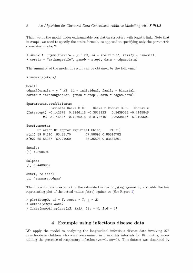
Then, we fit the model under exchangeable correlation structure with logistic link. Note thatin step1, we need to specify the entire formula, as opposed to specifying only the parametriccovariates in step2.

> step2 <- cdgam(formula = y ~ x3, id = individual, family = binomial,

+ corstr = "exchangeable", gamob = step1, data = cdgam.data)

The summary of the model fit result can be obtained by the following:

> summary(step2)

$call:cdgam(formula = y ~ x3, id = individual, family = binomial,corstr = "exchangeable", gamob = step1, data = cdgam.data)

$parametric.coefficients:Estimate Naive S.E. Naive z Robust S.E. Robust z

(Intercept) -0.142578 0.3946116 -0.3613122 0.3439056 -0.4145846x3 3.746447 0.7466218 5.0178646 0.6338137 5.9109591

$coef.smooth:Df exact Df approx empirical Chisq P(Chi)

s(x1) 59.84610 63.38170 47.58698 0.85314782s(x2) 65.55037 69.21069 86.35508 0.03634361

$scale:[1] 1.390494

$alpha:[1] 0.4480969

attr(, "class"):[1] "summary.cdgam"

The following produces a plot of the estimated values of f2(x2) against x2 and adds the linerepresenting plot of the actual values f2(x2) against x2 (See Figure 1):

> plot(step2, ci = T, resid = T, j = 2)

> attach(cdgam.data)

> lines(smooth.spline(x2, fx2), lty = 4, lwd = 4)

4. Example using infectious disease data

We apply the model to analysing the longitudinal infectious disease data involving 275preschool-age children who were re-examined in 3 monthly intervals for 18 months, ascer-taining the presence of respiratory infection (yes=1, no=0). This dataset was described by


0.0 0.2 0.4 0.6 0.8 1.0

original x-values for s(x2)

-4-2

02

eta

valu

e du

e to

s(x

2)

Figure 1: The plot of f̂2(x2) against x2 where f̂ is the estimation of f2(x2) where f2(x2) =cos(2.5πx2)/(1+3x2

2) with the dots representing the residuals, the solid dashed line representsf2(x2), the fine continuous line represents f̂2(x2), and the two fine dotted lines bounding f2(x2)and f̂2(x2) on either side represent the 95interval.

Zeger and Karim (1991) and has been used in Lin and Carroll (2001b) and Lin and Carroll(2001a) to perform generalized additive marginal modelling analyses. We have enclosed thisdataset, and called it indon. The description of each variable is as follows:

id Cluster identifier, where observations from thesame cluster share a common number.

res.infect Binary variable with presence of respiratoryinfecton=1, otherwise=0.

xeroph Presence of Vitamin A deficiency = 1,otherwise = 0.

cos.visit Seasonal cosine.sin.visit Seasonal sine.

sex Gender of the subject.height Height for age.stunt Presence of stunting.visit The number of visit when the observation was made.season 1=Spring, 2=Summer, 3=Autumn, 4=Winter.

age Age in years at the time of observation.baseline.age Age in years at the time of recruitment into study.

4.1. Initial phase of data modelling using GAM

Select part of the data for calculation:

> indon.sub <- indon[c(1:300),]


> length(unique(indon.sub[,1]))

[1] 71

There are 71 clusters in this subset.

Formulate the first step of modelling process using gam:

> step1 <- gam(formula = res.infect ~ s(age) + xeroph + cos.visit +

+ sin.visit + sex + height + stunt, family = binomial, x = T, data = indon.sub)

> summary(step1)

Call: gam(formula = res.infect ~ s(age) + xeroph + cos.visit +sin.visit + sex + height + stunt, family = binomial, data = indon.sub, x = T)Deviance Residuals:

Min 1Q Median 3Q Max-0.9851055 -0.6414985 -0.4321241 -0.2996751 2.709284

(Dispersion Parameter for Binomial family taken to be 1 )

Null Deviance: 253.6255 on 299 degrees of freedom

Residual Deviance: 228.4742 on 289.1412 degrees of freedom

Number of Local Scoring Iterations: 4

DF for Terms and Chi-squares for Nonparametric Effects

Df Npar Df Npar Chisq P(Chi)(Intercept) 1

s(age) 1 2.9 8.242089 0.03678064xeroph 1

cos.visit 1sin.visit 1

sex 1height 1stunt 1

Since the approximate nonparametric degree of freedoms for s(age) is 2.9, the step1 is re-fitted with s(age, df=3) so that it provides a better set of starting values of age for cdgam()formulation. step1 provides the starting values for model fitting in subsequent sections:

> step1 <- gam(formula = res.infect ~ s(age,df=3) + xeroph + cos.visit +

+ sin.visit + sex + height + stunt, family = binomial, x = T,data = indon.sub)

The degree of freedom for a nonparametric covariate is related to the smoothing parameterλ used in smooth.spline() called from gam(). When the nonparametric covariate is speci-fied as s(age), the smooth.spline() algorithm optimize the value of λ used in smoothing,


and it is reflected as the nonparametric degree of freedom. Hence, refitting the model byspecifying the nonparametric covariate as above using the specification s(age, df=3), thedegree of smoothing is controlled so that the value of λ used in gam() is that optimizedby smooth.spline(). We should refrain from using the nonparametric degree of freedomproduced with s(age, df=3) to refit using gam() because the aim is to obtain the optimalsmoothing for the nonparametric covariate age, as opposed to obtain the optimal smoothingfor the smoothed for of the nonparametric covariate with 3 degrees of freedom s(age, df=3).

4.2. Modelling under exchangeable correlation structure

We first fit the model assuming exchangeable correlation structure:

> step2.ex.1 <- cdgam(formula = res.infect~xeroph + cos.visit + sin.visit +

+ sex + height + stunt, id = id, family = binomial, corstr = "exchangeable",

+ gamob = step1, data = indon.sub)

> summary(step2.ex.1)

$call:cdgam(formula = res.infect ~ xeroph + cos.visit + sin.visit + sex + height +stunt, id = id, family = binomial, corstr = "exchangeable", gamob = step1,data = indon.sub)


(Intercept) -2.59349718 0.3184684 -8.14365674 0.26718656 -9.70669032xeroph 0.28062820 1.2883989 0.21781158 0.80096584 0.35036225

cos.visit -0.48070271 0.3361932 -1.42984087 0.28653001 -1.67766966sin.visit -0.23239116 0.3201893 -0.72579301 0.22724533 -1.02264439

sex -0.01935372 0.3939345 -0.04912928 0.31438041 -0.06156147height -0.05338726 0.0532786 -1.00203941 0.04880356 -1.09392144stunt -0.18177428 0.8179407 -0.22223407 0.67382854 -0.26976340


s(age, df = 3) 57.34003 62.75955 20.52969 0.9999969

$scale:[1] 1.473711

$alpha:[1] -0.03638948


Plotting the fitted function of age against age shows that the risk of respiratory infection isseen to increase until the age of 2, and then decrease after that. (See Figure 2)


> plot(step2.ex.1, ci = T, resid = T)

2 4 6

original x-values for s(age, df = 3)

-4-2

02

4

eta

valu

e du

e to

s(a

ge, d

f = 3

)

Figure 2: The plot of f̂age against age where the dots represent residuals from the indon datasubset estimated assuming exchangeable intracluster correlation structure, the fine continuousline represents estimated contribution to the risk of respiratory infection over age, and thetwo dotted fine lines its 95% confidence interval bound.

4.3. Modelling under AR(1) correlation structure

Fitting the model assuming an AR(1) correlation structure as it involves time factor, andspecifying the parameter visit as the correlation metameter:

> step2.ar1.1 <- cdgam(formula = res.infect~xeroph + cos.visit + sin.visit +

+ sex + height + stunt, id = id, cor.met = visit, family = binomial,

+ corstr = "ar1", gamob = step1, data = indon.sub)

> summary(step2.ar1.1)

$call:cdgam(formula = res.infect ~ xeroph + cos.visit + sin.visit + sex + height +stunt, id = id, cor.met = visit, family = binomial, corstr = "ar1",gamob = step1, data = indon.sub)





sex -0.09426448 0.37910997 -0.2486468 0.31784530 -0.2965735height -0.05628223 0.05030511 -1.1188174 0.04832306 -1.1647075stunt -0.19887753 0.77582578 -0.2563430 0.66140927 -0.3006875


s(age, df = 3) 55.90675 60.93737 15.06681 1

$scale:[1] 1.267612

$alpha:[1] -0.05534506


Plotting the fitted function of age against age shows there is over fitting due to a small valueof λ, retrievable from step2.ar1.1. (See Figure 3)

> plot(step2.ar1.1, ci = T, resid = T)

2 4 6


-6-4

-20

24

6

eta

valu

e du

e to

s(a

ge, d

f = 3

)

Figure 3: The plot of f̂age against age where the dots represent residuals from the indon datasubset estimated assuming AR(1) intracluster correlation structure with λ = 4.478831×10−6,the fine continuous line represents estimated contribution to the risk of respiratory infectionover age, and the two dotted fine lines its 95% confidence interval bound.

Therefore, a new value for λ is specified, arbitrarily set as 10 times that in step2.ar1.1 anda new model is fitted. (See Section 5 for the rationale of such choice of factor of expansionfor λ)


> step2.ar1.1$lambda

[[1]]:[1] 4.478831e-006

> lambda.new <- 10*unlist(step2.ar1.1$lambda)

> step2.ar1.2 <- cdgam(formula = res.infect~xeroph + cos.visit + sin.visit +

+ sex + height + stunt, id = id, lambda=lambda.new, cor.met = visit,

+ family =binomial, corstr = "ar1", gamob = step1, data = indon.sub)

The summary results of model fit with the new smoothing parameter λ’ is as follows:

> summary(step2.ar1.2)

$call:cdgam(formula = res.infect ~ xeroph + cos.visit + sin.visit + sex + height +stunt, id = id, lambda = lambda.new, cor.met = visit, family = binomial,corstr = "ar1", gamob = step1, data = indon.sub)




sex -0.07251887 0.3741501 -0.1938229 0.3198790 -0.2267072height -0.05315972 0.0495429 -1.0730039 0.0470079 -1.1308678stunt -0.32053131 0.7654951 -0.4187242 0.6768653 -0.4735526


s(age, df = 3) 40.20359 41.77025 54.38034 0.05418916

$scale:[1] 1.242216

$alpha:[1] -0.04773346


Plotting the fitted function of age against age shows a reasonable degree of roughness penalty.(See Figure 4)

> plot(step2.ar1.2, ci = T, resid = T)


2 4 6


-6-4

-20

24

eta

valu

e du

e to

s(a

ge, d

f = 3

)

Figure 4: The plot of f̂age against age where the dots represent residuals from the indondata subset estimated assuming AR(1) intracluster correlation structure with λ′ = 10× λ =4.478831 × 10−5, the fine continuous line represents estimated contribution to the risk ofrespiratory infection over age, and the two dotted fine lines its 95% confidence interval bound.

2 4 6


-10

12

eta

valu

e du

e to

s(a

ge, d

f = 3

)

Figure 5: The plot of f̂age against age where the dots represent residuals from the indondata subset estimated assuming AR(1) intracluster correlation structure with λ′ = 10× λ =4.478831 × 10−5, the fine continuous line represents estimated contribution to the risk ofrespiratory infection over age, and the two dotted fine lines its 95% confidence interval bound.


Plotting the fitted function of age against age without standard error bands and residualsallows a closer inspection of the trend of respiratory infection risk against age. (See Figure 5)The risk of respiratory infection is noted to increase since birth to 2 years old, and thendecreases thereafter. Similar observation is reported in Figures 3 and 4 of Lin and Carroll(2001b).

> plot(step2.ar1.2)

Due to the slow convergence rate, modelling for step2.ex.1, step2.ar1.1, and step2.ar1.2,require up to 6 back-fitting loops, and up to 200 Gauss-Seidel interations within each loop.

References

Berhane K, Tibshirani RJ (1998). “Generalized Additive Models for Longitudinal Data.” TheCanadian Journal of Statistics, 26, 517–535.

Chambers JM, Hastie TJ (1993). Statistical Models in S. Chapman and Hall, London.

Green PJ, Silverman BW (1994). Nonparametric Regression and Generalized Linear Models.Chapman and Hall, London.

Hastie TJ, Tibshirani RJ (1990). Generalized Additive Models. Chapman and Hall, London.

Lee AJ (1993). “Generating Random Binary Deviates Having Fixed Marginal Distributionand Specified Degrees of Association.” The American Statistician, 47, 209–215.

Liang KY, Zeger SL (1986). “Longitudinal Data Analysis Using Generalized Linear Models.”Biometrika, 73, 13–22.

Lin X, Carroll RJ (2001a). “Semiparametric Regression for Clustered Data.” Biometrika, 88,1179–1185.

Lin X, Carroll RJ (2001b). “Semiparametric Regression for Clustered Data Using GeneralizedEstimating Equations.” Journal of American Statistical Association, 96, 1045–1056.

Lin X, Wang N, Welsh AH, Carroll RJ (2004). “Equivalent Kernels of Smoothing Splines inNonparametric Regression for Clustered/Longitudinal Data.” Biometrika, 91, 177–193.

McCullagh P, Nelder JA (1989). Generalized Linear Models. Chapman and Hall, London.

Ruppert D (1997). “Empirical-Bias Bandwith for Local Polynomial Nonparametric Regressionand Density Estimation.” Journal of American Statistical Association, 92, 1049–1062.

Zeger SL, Karim MR (1991). “Generalized Linear Models with Random Effects: A Gibb’sSampling Approach.” Journal of American Statistical Association, 86, 79–86.


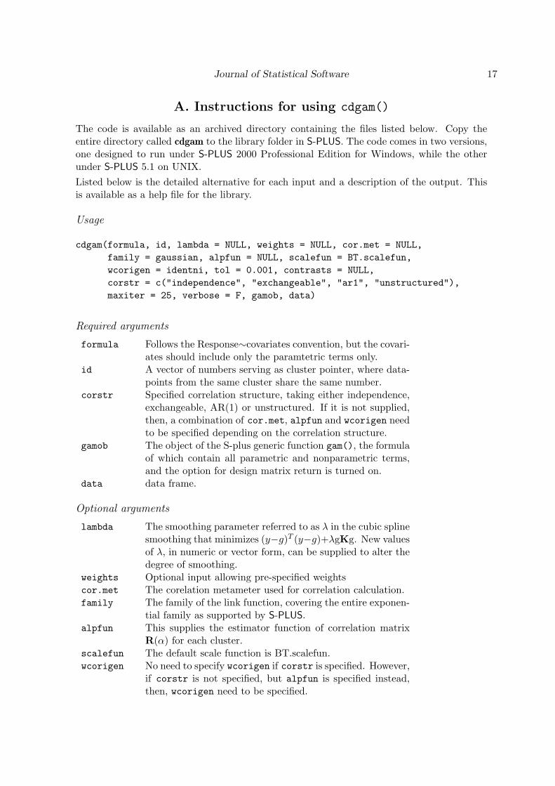
A. Instructions for using cdgam()

The code is available as an archived directory containing the files listed below. Copy theentire directory called cdgam to the library folder in S-PLUS. The code comes in two versions,one designed to run under S-PLUS 2000 Professional Edition for Windows, while the otherunder S-PLUS 5.1 on UNIX.Listed below is the detailed alternative for each input and a description of the output. Thisis available as a help file for the library.

Usage

cdgam(formula, id, lambda = NULL, weights = NULL, cor.met = NULL,family = gaussian, alpfun = NULL, scalefun = BT.scalefun,wcorigen = identni, tol = 0.001, contrasts = NULL,corstr = c("independence", "exchangeable", "ar1", "unstructured"),maxiter = 25, verbose = F, gamob, data)

Required arguments

formula Follows the Response∼covariates convention, but the covari-ates should include only the paramtetric terms only.

id A vector of numbers serving as cluster pointer, where data-points from the same cluster share the same number.

corstr Specified correlation structure, taking either independence,exchangeable, AR(1) or unstructured. If it is not supplied,then, a combination of cor.met, alpfun and wcorigen needto be specified depending on the correlation structure.

gamob The object of the S-plus generic function gam(), the formulaof which contain all parametric and nonparametric terms,and the option for design matrix return is turned on.

data data frame.

Optional arguments

lambda The smoothing parameter referred to as λ in the cubic splinesmoothing that minimizes (y−g)T (y−g)+λgKg. New valuesof λ, in numeric or vector form, can be supplied to alter thedegree of smoothing.

weights Optional input allowing pre-specified weightscor.met The corelation metameter used for correlation calculation.family The family of the link function, covering the entire exponen-

tial family as supported by S-PLUS.alpfun This supplies the estimator function of correlation matrix

R(α) for each cluster.scalefun The default scale function is BT.scalefun.wcorigen No need to specify wcorigen if corstr is specified. However,

if corstr is not specified, but alpfun is specified instead,then, wcorigen need to be specified.


tol The tolerance limit defining convergence of the local scoringprocedure.

contrasts Optional entry for constrast can be supplied here.maxiter The maximum local scoring iterations allowed by default is

25.verbose logical.

Details

Corresponding cor.met for each correlation structure is as below:

Correlation structure cor.metexchangeable need not specifystratified exchangeable a vector of numbers serving as

cluster pointer, identical to theentry for input id.

AR(1)-evenly spaced time scale a vector the times at which thecorresponding data points wererecorded.

AR(1)-unevenly spaced time scale a matrix with two columns; thefirst being the cluster pointer,the second the times at which thecorresponding data points wererecorded.

unstructured a vector providing the meansfor selecting appropriateelements for incomplete clustersfrom the time-saturatedcorrelation matrix.

Corresponding alpfun for each correlation structure is as below:

Correlation structure alpfunexchangeable BT.exchalpstratified exchangeable BT.strat.exchalpAR(1)- evenly spaced time scale BT.prop.ar1alpAR(1)- unevenly spaced time scale LZ.ar1alpunstructured BT.prop.unstruc.alpindependence (no need to specify)

Corresponding wcorigen for each alpfun is as below:

alpfun wcorigenBT.exchalp excoriput or excoriBT.strat.exchalp strat.excoriputBT.prop.ar1alp ar1.coriputLZ.ar1alp LZ.ar1.coriputBT.prop.unstruc.alp unstr.coriputindependence (no alpfun needed) identni


Output

The output is a list containing the following elements:

para output from cdgam.par()pertaining to the parametric portion of themodelling process

nonparametric output from cdgam.nonpar()pertaining to the nonparametric portion ofthe modelling process

lambdaK the product of the smoothing parameterand the cubic spline basis matrices (Green &Silverman pp 13)

lambda the value(s) of the smoothing parameterused in smoothing

x.smooth the covariates requiring smoothing. Whenmore than one, it is ordered by column fromleft to right as appeared in the formulasupplied in gam(..., x = T).

incidence.matrix the list of incidence matrices used byeach nonparametric term that allow for ties(Green & Silverman pp 65)

final.eta the smoothed values of the nonparametricterms. When more than one, it is ordered bycolumn from left to right as appears in theformula supplied in gam(..., x = T).

call the call that produce the results

The para portion of the output contain the followings:

coefficients Values of the coefficients for theparametric terms at local convergence

naive.parmvar the product of the scale parameter andthe variance matrix

robust.parmvar the sandwich estimate of variancealpha correlation parameter(s)phi scale parameterlinear.predictors eta values for the parametric portionfitted.values mu values for the parametric portion,

i.e., g(µ) = η.pearson.resid Pearson’s residualsiter number of Fisher’s scoring loop for the

last local scoring iteration at convergence.family the family of the link function


rank the number of parametric parameters inthe cdgam.par() fitting

errorcode the error messages generated duringcalculation of cdgam.par()

Rinv.i the list containing inverse of theworking correlation matrix for each clusterto be used in cdgam.nonpar()

MX the matrix containing all covariatesinformation, by column, as ordered in theformula of gam(..., x = T).

b0 fitted values of beta, the coefficientsfor the parametric terms

The nonparametric portion of the output contain the followings:

T.s.emp Empirical calculation of chi-squaredvalues for nonparametric terms (Berhane &Tibshirani Section 4.2)

T.s.mb Model-based calculation of chi-squaredvalues for nonparametric terms (Berhane &Tibshirani Section 4.2)

T.s.chisq p-value for chi-squared based onapproximate degrees of freedom (Berhane &Tibshirani Section 4.2)

df.nl Degree of freedom according to Berhane &Tibshirani Equation 8.

df.approx Degree of freedom approximated by1.25trace(S)-0.5.

eta.nonpar Sum of eta values for smoothing term(s)for each observation point.

se.emp Empirical calculation of standard error(Berhane & Tibshirani Equation 26)

se.mb Model-based calculation of standard error(Berhane & Tibshirani Equation 25)

smooth.terms Matrix containing individual eta for eachsmoothed term, the addition of which by row-wise produces eta.nonpar

smoother Smoother matrix for each smoothing termat convergence

weight Weight matrices at convergenceA.nonpar Variance matrix (q × q)V.nonpar sandwich estimate of variance

(non-parametric form of Berhane & TibshiraniEquation 4)

V.inv inverse of V.nonpar


B. Instructions for using plot.cdgam()

Usage

plot(x, ci.option = c("mb", "emp"), j = NULL, ci = F, resid = F)

Required arguments

x The fitted object from class cdgam

Optional arguments

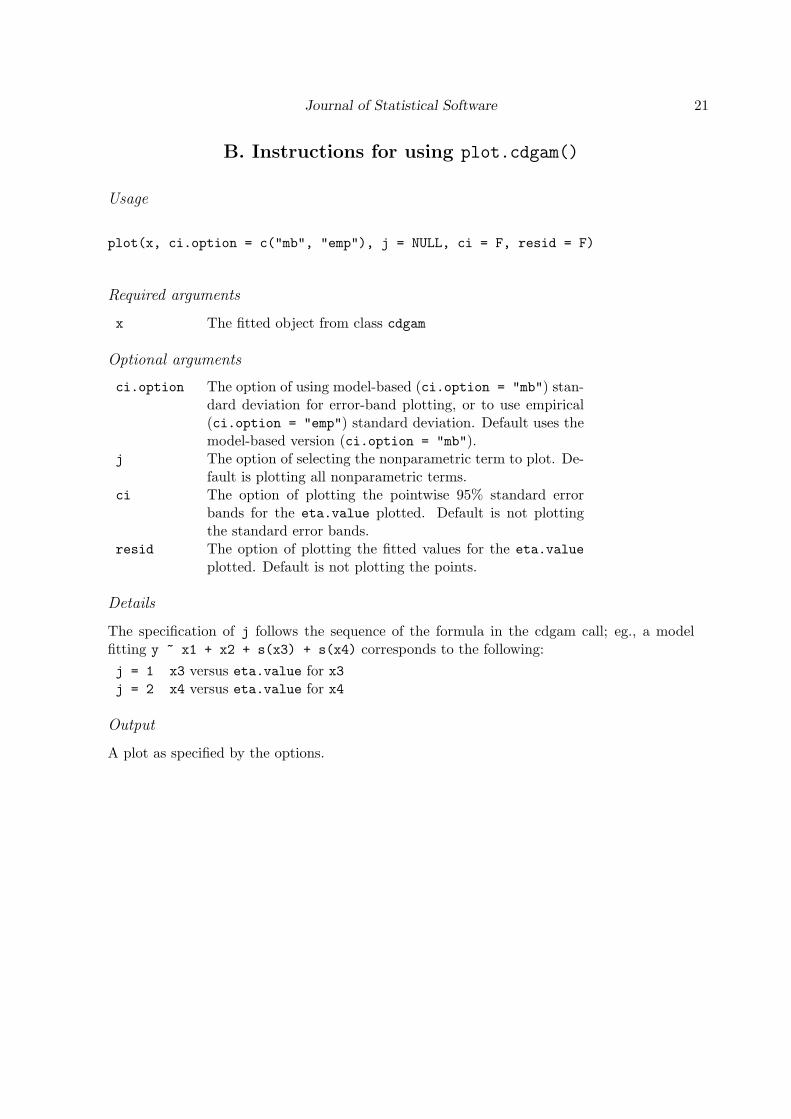
ci.option The option of using model-based (ci.option = "mb") stan-dard deviation for error-band plotting, or to use empirical(ci.option = "emp") standard deviation. Default uses themodel-based version (ci.option = "mb").

j The option of selecting the nonparametric term to plot. De-fault is plotting all nonparametric terms.

ci The option of plotting the pointwise 95% standard errorbands for the eta.value plotted. Default is not plottingthe standard error bands.

resid The option of plotting the fitted values for the eta.valueplotted. Default is not plotting the points.

Details

The specification of j follows the sequence of the formula in the cdgam call; eg., a modelfitting y ~ x1 + x2 + s(x3) + s(x4) corresponds to the following:j = 1 x3 versus eta.value for x3j = 2 x4 versus eta.value for x4

Output

A plot as specified by the options.


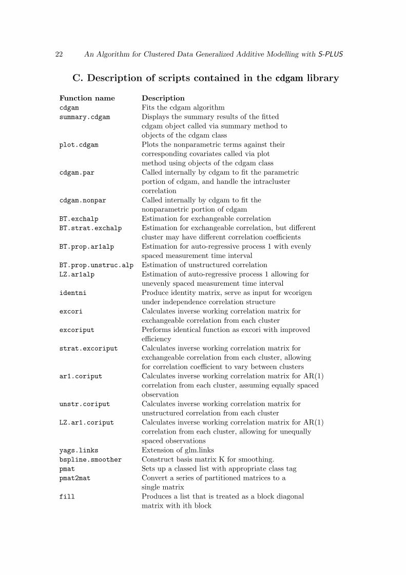
C. Description of scripts contained in the cdgam library

Function name Descriptioncdgam Fits the cdgam algorithmsummary.cdgam Displays the summary results of the fitted

cdgam object called via summary method toobjects of the cdgam class

plot.cdgam Plots the nonparametric terms against theircorresponding covariates called via plotmethod using objects of the cdgam class

cdgam.par Called internally by cdgam to fit the parametricportion of cdgam, and handle the intraclustercorrelation

cdgam.nonpar Called internally by cdgam to fit thenonparametric portion of cdgam

BT.exchalp Estimation for exchangeable correlationBT.strat.exchalp Estimation for exchangeable correlation, but different

cluster may have different correlation coefficientsBT.prop.ar1alp Estimation for auto-regressive process 1 with evenly

spaced measurement time intervalBT.prop.unstruc.alp Estimation of unstructured correlationLZ.ar1alp Estimation of auto-regressive process 1 allowing for

unevenly spaced measurement time intervalidentni Produce identity matrix, serve as input for wcorigen

under independence correlation structureexcori Calculates inverse working correlation matrix for

exchangeable correlation from each clusterexcoriput Performs identical function as excori with improved

efficiencystrat.excoriput Calculates inverse working correlation matrix for

exchangeable correlation from each cluster, allowingfor correlation coefficient to vary between clusters

ar1.coriput Calculates inverse working correlation matrix for AR(1)correlation from each cluster, assuming equally spacedobservation

unstr.coriput Calculates inverse working correlation matrix forunstructured correlation from each cluster

LZ.ar1.coriput Calculates inverse working correlation matrix for AR(1)correlation from each cluster, allowing for unequallyspaced observations

yags.links Extension of glm.linksbspline.smoother Construct basis matrix K for smoothing.pmat Sets up a classed list with appropriate class tagpmat2mat Convert a series of partitioned matrices to a

single matrixfill Produces a list that is treated as a block diagonal

matrix with ith block


sum.pmat Sum over structuresum.pmat.block Sum over structuresolve.pmat Inverse the structuresolve.pmat.block Inverse the structuresolve.pmat.block.default Inverse the structuresolve.pmat.block.diag Inverse the structuret.pmat Transpose the structuret.pmat.block Transpose the structuredet Calculate determinant of structuredet.default Calculate determinant of structuredet.pmat Calculate determinant of structuredet.pmat.block Calculate determinant of structuredet.pmat.block.default Calculate determinant of structuredet.pmat.block.diag Calculate determinant of structurecdim Assignment of attribute to object in support of pmat2matrdim Assignment of attribute to object in support of pmat2matmsplit Convert a matrix to a partitioned matrixdist2full Matrix manipulation for lower trianglefull2tri & tri2full Matrix manipulation for lower trianglesplit.preserveord Create pointer for partitioningload.clustered.design Partition the design matrixload.clustered.outcome Partition the response variableload.bd.weight Partition the weight vectorvsplit General function for matrix partitiontransfer.matfun Support load.clustered.design and

load.clustered.outcome for matrix partitioncdgam.data Data set for Section 9indon Actual dataset for Section 10ngau.m2ll Evaluates 2 times the Gaussian log likelihood of

the residualsgau.hetex.alp Script asssignment for alp optional argument in

cdgam to model Gaussian estimation for correlationparameters

nexinv Analytic form of inverse of compound symmetry matrixmake.exch.cor.genarg Script to support calculation of inverse working

correlation matrix for Gaussian estimation forcorrelation parameters

exch.cor Function in conjunction with make.exch.cor.genargexch.gaussian.loglik Function in conjunction with make.exch.cor.genarg


Affiliation:

Lin Yee HinPrivate Medical PractitionerHong KongE-mail: [email protected]

Vincent CareyAssociate Professor of Medicine (Biostatistics)Harvard Medical SchoolChanning Laboratory181 Longwood Ave Boston MA02115 USAE-mail: [email protected]

Journal of Statistical Software Submitted: 2005-01-27August 2005, Volume 14, Issue 8. Accepted: 2005-08-31http://www.jstatsoft.org/

mailto:[email protected]

mailto:[email protected]

http://www.jstatsoft.org/

Date post:	25-Feb-2022
Category:	Documents
Upload:	others
View:	6 times
Download:	0 times

An Algorithm for Clustered Data Generalized Additive

Documents