An analysis of bidding strategies in the Danish wind power market En analyse av strategisk budgivning i det danske vindkraftmarkedet Norwegian University of Life Sciences Faculty of Social Sciences School of Economics and Busines Master Thesis 2014 30 credits Nabeela Qureshi brought to you by CORE View metadata, citation and similar papers at core.ac.uk provided by NORA - Norwegian Open Research Archives
Transcript
An analysis of bidding strategies in the Danish wind power market En analyse av strategisk budgivning i det danske vindkraftmarkedet
Norwegian University of Life Sciences Faculty of Social Sciences School of Economics and Busines
Master Thesis 2014 30 credits
Nabeela Qureshi
brought to you by COREView metadata, citation and similar papers at core.ac.uk
provided by NORA - Norwegian Open Research Archives
3.1.1 Model 1 ......................................................................................................................... 16
3.1.1.1 Modification of Model 1 .......................................................................................... 18
3.1.2 Model 2 ......................................................................................................................... 19
3.1.3 Hypotheses and model summary .................................................................................. 22
4 Data .............................................................................................................................................. 25
4.1 The variables ........................................................................................................................ 25
Appendix 1 ............................................................................................................................................. A
Appendix 2 ............................................................................................................................................. C
Appendix 3 ............................................................................................................................................. E
X
List of Figures Figure 1: Wind power capacity and wind-power’s share of domestic supply (Jensen & Sørensen 20014). .......... 9 Figure 2: Price of regulating power (Skytte 1999). .............................................................................................. 17 Figure 3: Daily up and down regulation. .............................................................................................................. 34 Figure 4: Distribution of the variable total regulation. ......................................................................................... 35
List of Figures Table 1: Descriptive statistics of the variables. .................................................................................................... 27 Table 2: Estimated parameters model 1. ............................................................................................................... 31 Table 3: Estimated parameters OLS, OLS_Proxy, 2SLS ..................................................................................... 36
XI
XII
1 Introduction
An analysis of bidding strategies in the Danish power market “This asymmetric cost may encourage bidders with fluctuating production to be more
strategic in their way of bidding on the spot market. By using such strategies the extra costs for e.g. wind power needed to counter unpredictable fluctuations may be limited”
(Skytte 1999)
How does deviation between predicted production and actual production of wind-power in West-Denmark affect the bidding in the spot market?
1.1 Background
This thesis is inspired by the quote presented above, taken from Klaus Skytte's article “The
regulating power market on the Nordic power exchange, Nord Pool” published in 1999. His
research and findings suggest that the cost of using the regulation power market is dependent
on the spot price level at the Nordic power exchange. He discovered that the regulation cost
was more correlated to the spot price in an event of down-regulation, compared an event of
up-regulation. With expected fluctuation of supply and demand, the actor in the market is
able to jointly optimize his total bids at the spot market and in the regulation market (Skytte
1999). His research targeted Norwegian hydropower producers.
Skytte's article was written before Denmark joined the Nordic power exchange, Nord Pool, in
year 2000 (NordPool 2013). Today Denmark's wind power production covers 30 % of the
country´s energy production. An analysis of the current effects of the wind power supply bids
submitted in Nord Pool may provide insights that can determine the hidden cost or as Skytte
described, strategic bidding behaviour related to fluctuating power supply. Within year 2020
wind energy production is planned to increase, and will account for 50 % of the total energy
production in Denmark (Danish Wind Industry Association 2014). According to these plans
the amount of wind power in the system will increase. A research on wind power production
in West-Denmark and up- regulation was published in 2007, the article concluded the
1
relation as significant (Forbes et al. 2007). By using updated data from 2012-2013 and
modified version of the model discussed in Skytte's article the goal of this thesis is to detect
any indication of strategic behaviour in the Danish wind power market, by analysing the
bidding strategies related to wind power supply. The bidding area of interest is West-
Denmark, and their use of regulation services.
It seems like that the suspicion of strategic behaviour lies in the bidding behaviour of the
wind power producers. The suspicion is that they systematically bid less wind power supply
than the predicted amount, and then use the regulation market to down regulate the excess
supply. If asymmetries are found in the regulation market, further analysis of this thesis will
test the regression model for systematic measurement error. Whether systematic behaviour is
an economic burden or has any spillover effects on other actors in the market will depend on
the magnitude of the problem, and is not discussed in this thesis. This thesis will focus on
indirect evidence of strategic behaviour in the bidding area of West-Denmark.
1.2 Problem for discussion
How does deviation between predicted production and actual production of wind-power in West-Denmark affect the bidding in the spot market?
The interest here is to use the regulation market and the wind prognosis to find the deviations
between supply bids made at the spot market, and actual delivery. There is no official data on
the bids submitted into Nord Pool, as the data is confidential. Therefore problem stated will
be answered without using this data, and the problem for discussion will be answered based
on these hypotheses:
Hypothesis one: There is no systematic relationship between regulation price, and up or
down- regulation.
The alternative hypothesis is that there is a systematic relationship between regulation price
and up or down-regulation.
Hypothesis two: Wind power production is an exogenous predictor of total regulation
2
The alternative hypothesis will reject hypothesis two and state that wind power production is
endogenous and measured with error.
1.3 Structure
The first chapter of this thesis reveals the problem for discussion and the related hypotheses
to be tested. The second chapter provide an overview of Nord Pool, earlier research on
strategic behaviour in the power market, and the Danish bidding areas. In the third chapter,
the two models behind the analysis are introduced with the relevant indication of the theory
behind them. The data and variables used in the analysis of the models are given in chapter
four. In chapter five the estimation, strategy and the analysis structure are given. The results
are specified and discussed in chapter six before concluding remarks in the final chapter.
3
This page intentionally left blank.
4
2 Nord Pool and strategic behaviour
This chapter is divided into four sections. Firstly the conceptual framework behind the
Nordic electricity market is presented. Secondly the Danish power market, bidding areas and
their future investment plans is discussed in the second part. In the third part of this chapter,
the earlier research on strategic behaviour is discussed before a brief chapter summary is
provided.
2.1 The Nordic electricity exchange
Nord Pool is the Nordic electricity exchange with member countries Denmark, Norway
Sweden, Finland, Estonia, and Lithuania. Electricity Producers, retailers, traders, and large
end users meet in the Nord Pool spot exchange to trade electricity. The producers need to pay
a fee to the grid owner for each kWh they pour into the grid, and the consumers need to pay a
fee for each kWh they draw from the grid. This is known as the point tariff system. This
system is relevant for understanding the key balance between production and consumption in
the system every hour (Nord Pool 2014a).
Each hour somewhere in the system the producer has to produce a certain amount of
electricity to the grid, and that same amount has to be consumed by the retailer´s customers.
Electricity grids transport the power, and for each local grid, there is a local grid operator
who handles the local low voltage grid. The TSO owns and operates the high voltage grid for
the respective country. Because the TSO own and operates the grid, it is solely responsible
for the assurance of supply in the country they are operating. The Danish TSO is
Energinet.dk, and it is a state-owned grid-company for both gas and electricity (Nord Pool
Here, 𝑃𝑅𝑡 is the regulation price for balancing regulation and V is the actual volume of
regulation. Subscripts up and do stand for up and down- regulation. More information about
the variables is provided in chapter four.
Finally, equation (9) is studied through creating a graph. Here the change in price of
balancing regulation is given as the difference in price of up and down-regulation in the
relevant time period.
Δ𝑃𝑡𝑟 = 𝑃𝑡𝑢𝑝 − 𝑃𝑡𝑑𝑜 (9)
This modified version of Skytte's model is regarded as model 1 hereafter, because this
version of the model is relevant for the analysis.
3.1.2 Model 2
Model 2 is based on econometric theory of measurement error in the model. The estimation
method is used because there is a suspicion of endogeneity in the model. The use of proxy
variable and the use of an instrumental variable are methods used to correct for endogeneity,
given that the OLS1 estimation may not produce good results. In this case there is a
suspicion of endogeneity in the model, related to the variable of wind power production. The
objective is to check the model for endogeneity and signs of systematic measurement error
that can be linked to strategic behaviour. In Model 2, the dependent variable in the regression
1 The method of ordinary least squares
19
is total regulation, and the independent variables are net exports, wind power production and
total power production. The failure of meeting total demand at the time of actual delivery is
reflected in total regulation. The goal is to extract the effect of planned wind power
production on total regulation.
When there is endogeneity in the independent variables, the results will be produced with
bias estimates. Endogeneity can be caused by omitted variables, measurement error or
simultaneity. Possible ways to correct for unobserved endogeneity is to find a suitable proxy
for the unobserved variable. The instrumental variables regression approach can also be
applied. The use of OLS in presence of endogeneity will lead to a correlation between the
explanatory variables and the error term, and results will be biased. In this case, the
unobserved part of the model is the strategic element added to the planned wind power
production. The assumption is that this strategic element will be detected through the
endogeneity in the independent variable and this can be classified as systematic measurement
error (Reichstein 2011).
The assumption in the classical linear regression model is that the model is being measured
with an error term 𝜀. The problem of measurement error distinguishes from the error term 𝜀,
because the assumption here is that in addition to the error term of the model, the
independent variable is being measured with an error. The models with measurement errors
follow, the key assumption that the response variable and the predictor variables are subject
to additive measurement errors. The regression model in this case is subject to an unknown
constant, which classify the model to become a functional measurement error model (Young
2014).
In presence of a measurement error the estimation method of 2SLS2 can be applied to correct
for the error. In the model X is an independent variable, Y is dependent variable and Z is the
instrumental variable. The instrumental variable Z affects the dependent variable Y, only
through its effect on the independent variable X. (Young 2014). Two properties must be
satisfied in order to for the instrumental variable to be consistent. The instrumental variable
must be relevant and strong. In order to be relevant, there must be a strong correlation
2 Two-stage least-squares
20
between the IV and the independent variable it is instrumenting for. The IV must be
uncorrelated with the error term, and by that, the IV is exogenous (Young 2014).
The Hausman test is a specification test for measurement error with the null hypothesis of no
measurement error. Under this hypothesis, both the OLS estimator and the instrumental
variable estimators are consistent estimators in the model. The OLS will be efficient, and the
instrumental variable estimator will be inefficient if the null hypothesis is valid. On the other
hand, if the null hypothesis is rejected, the instrumental variable estimator will be consistent,
and not the OLS estimator. In brief, the Hausman test is used to compare the result from the
OLS and the 2SLS (Green 1990).
To improve OLS results, the OLS can be estimated using a proxy variable. There is
difficulties related to the measure corresponding to the variable 𝑊𝑡𝑃, but still this variable is
defined in the regression. There are observable indicators for this variable, and in this context
the variable wind prognosis, 𝑊𝑡𝑃𝑟𝑜𝑔, will be regarded as an indirect measure of 𝑊𝑡
𝑃.
Theoretically, it is highly unlikely that an improvement in the measurement will bring the
proxy closer to the variable, which it is a proxy for (Green 1990).
In context of the theory given above, Model 2 is designed. The objective of Model 2 is to
find the effect of 𝑊𝑡𝑃 on the total regulation amount. The unobservable variable 𝑊𝑡
𝑃 from
equation (1) will be measured indirectly as this information is missing. What is known is that
wind power production is solely dependent on the amount of wind that enters the system. To
analyse what happens when the supply bid is planned, wind fluctuations are considered. The
effect of planned wind power production on total regulation is the basis for the regression
estimation in Model 2.
Without the strategic element in the model, the assumption is as following:
𝑊𝑡𝑃 = 𝑊𝑡
𝐴𝐶 = 𝑊𝑡 (10)
Ideally, total regulation should be regressed against all the independent variables from
equation (4) to obtain the effect of planned wind power production on total regulation:
𝑅𝑡 = 𝛽0 + 𝛽1𝑄𝑡 + 𝛽2𝑋𝑡 + 𝛽3𝑊𝑡 + 𝜀𝑡 (11)
21
The introduction of an instrumental variable will attempt to solve the missing variable
problem, and the variable wind power prognosis is used as an instrument in the 2SLS:
𝑅𝑡 = 𝛼𝑡 + 𝑄𝑡 + 𝑋𝑡 + 𝑊𝑡𝑃𝑟𝑜𝑔 + 𝜀𝑡 (12)
To be able to compare the OLS estimation with planned wind power production included,
wind prognosis is tested as a proxy variable for actual wind power production, and equation
(13) becomes the following:
𝑤𝑡𝐴𝐶 = 𝛼 + 𝑤𝑡
𝑝𝑟𝑜𝑔 + 𝜀𝑡 (13)
The OLS estimation with a proxy variable is as showed in equation (14):
𝑅𝑡 = 𝛽0 + 𝛽1𝑄𝑡 + 𝛽2𝑋𝑡 + 𝛽3𝑊𝑡𝑃 + 𝛽4𝑊𝑡
𝑃𝑟𝑜𝑔𝑡 + 𝜀𝑡 (14)
Lastly, the Wu-Hausman test for endogeneity is applied to compare OLS and 2SLS results.
The OLS estimation and the OLS estimation with a proxy are compared using the Likelihood
ratio test. This test shows the improvements in the estimation by using a proxy variable.
3.1.3 Hypotheses and model summary
Hypothesis one: There is not a systematic relationship between regulation price, and up or down regulation
Hypothesis two: Wind power production is exogenous predictor of total regulation
Model 1 and Model 2 is applied in order to answer the problem of discussion. Model 1 is
estimated first, and if the results suggest that asymmetries are found, Model 2 continues the
research by specifically testing the relationship between total regulation and wind power
production, because the suspicion is that the asymmetries in the regulation market is caused
by the deviations between planned and actual wind power production. Hypothesis one is
tested in Model 1, and after the results are conducted from Model 1, hypothesis two is tested
in Model 2. To sum up, to state the problem for discussion the deviations between actual and
22
planned wind power production will be tested by the effect of wind power prognosis on total
regulation. Further, the direct effect on the bidding strategy cannot be obtained, as the data
on the actual bid is confidential. The way of analysing the bidding structure in this research
will be done by examining if there are any incentives for wind power producers to
systematically use the regulation market to preserve their interests in the spot market.
Significant measurement error may be indirect evidence on systematic action and therefore
Model 2 is tested for endogeneity.
23
This page left intentionally blank.
24
4 Data
The data used in the model 1 and model 2 is downloaded from energinet.dk, except the data
on wind prognosis which is downloaded from Nord Pool´s website. Energinet.dk updates the
homepage twice each day, and uses the latest data in update. The measurement unit and
currency unit for price is Euro per MWh. The data downloaded is from 01.01.2012 to
31.12.2013. Which is a total amount of 24 months and 17544 observations on an hourly
basis.
In general, the dataset the observations regard for 24 hours per day, but there is one particular
day in March reported with 23 hours. This happens because the time changes from
wintertime to summertime (Nielsen 2010). In the time period from 01.01.2012 to 31.12.2013,
these dates occur at 25th march 2012, and 31st March 2013, which lead to that the 3rd hour
was blank on these dates. The blank area in the data set is corrected for by filling in the data
from hour four. The mean value of hour 2 and 4 could also have been used, but the values of
these hours were very similar, so the mean value was not used to fill in for the missing hour.
When summertime changes to wintertime, in general one day will be calculated as 25 hours,
because the 3rd hour will be calculated twice (Nielsen 2010). In the dataset all of the
observations fit the time series setting from 1 to 24, therefore no 25th hour was observed.
4.1 The variables
All the observable variables used in Model 1 and 2 are in the dataset. The Elspot price for
DK-West (West-Denmark) is used as the price variable for DK-West bidding area. DK-West
primary and local production generates the variable of total production in DK-West. DK-
West wind production is treated as one variable, and not as a part of total production.
Upward and downward regulation for DK-West, both amount and price are important and
included in the dataset. In addition there is a price for balancing power consumption, which
in the analysis is shortened to price for balancing regulation, and this is regarded as the
25
regulation price. Down regulation values are given with a negative sign, and up regulation
values are given with positive signs. DK-West trades power with Norway, Sweden and
Germany, and data on trade with all the three countries is included to create one net export
variable in the analysis. The trade with East-Denmark is not considered in this variable.
Observations have either positive or negative values to distinguish between import and
export. A detailed description of how these variables are generated is given in chapter five.
4.2 Descriptive statistics
Descriptive statistics of all variables is presented in table 1. The standard deviation of total
regulation, net exports, wind prognosis and wind production is high compared to the other
variables. There are huge differences between the minimum and maximum values for all
variables. Up and down regulation have fewer observations than the other variables, because
the observation is done only for those hours when up and down -regulation takes place. Total
production has the highest mean value, and the mean value of the wind power production and
wind prognosis is very similar. The coefficient of variance is equal for wind power
production and wind prognosis. Total regulation has the highest value of the coefficient of
variance. The mean value of price for up-regulation is higher compared to down- regulation.
DK-West area price has a mean value between the mean values of up and down regulation
price.
26
Table 1: Descriptive statistics of the variables.
Variable N Mean Std-dev Median Min Skewness CV Max
Total regulation 17544 1.51 93.09 0.00 -704.70 0.21 61.58 714.90 Total production 17544 1498.32 662.59 1397.70 355.80 0.61 0.44 4062.40 Net exports 17544 135.83 660.31 174.80 -2226.30 -0.31 4.86 1896.30 Wind prognosis 17544 919.09 739.63 709.00 11.00 0.92 0.80 3323.00 Price of balancing 17544 37.21 23.90 34.36 -217.01 3.73 0.64 499.93 Wind production 17544 929.37 744.33 738.50 0.60 0.84 0.80 3871.10 Down regulation 5230 -82.51 80.51 -55.00 -704.70 -2.12 -0.98 -0.50 Up regulation 4492 101.97 89.48 81.10 0.40 1.57 0.88 714.90 Price for down regulation 17544 32.78 14.99 32.95 -217.01 -1.74 0.46 183.39 Price for up regulation 17544 42.08 39.31 37.67 -199.99 33.00 0.93 1999.89 Spot price DK-West 17544 37.66 35.24 36.15 -200.00 44.92 0.94 2000.00
27
This page intentionally left blank.
28
5 Estimation and analysis
All statistical analysis was conducted using the STATA3 software version 13. The data
described in chapter four was divided into two datasets, one for each model. Some variables
are repeated and appear in both datasets. For model 1 data is analysed in STATA as hourly
time series with time variable hour running from 1 to 17544. The results are established on
based on these 17544 hours only. Time series variable are tested for stationarity using the
Augmented Dickey- Fuller (ADF) unit root test are found to be stationary, see appendix 1 for
details
Model 1 is estimated first. Two dummy variables are generated one for up- regulation and the
other for down- regulation. The dummy variables are multiplied with the area price of DK-
West to generate two new variables as required in the model. The dummy variable for up-
regulation is multiplied with up-regulation volume, and similarly the down-regulation
dummy is multiplied with down-regulation volume. Model 1 requires all of these variables
for the regression analysis.
At first Model 1 is estimated using ordinary least square (OLS). Specification tests conducted
on OLS results indicate the need to control for autocorrelation and heteroscdasticity. To
control for autocorrelation and heteroscedasticy, the model was re-estimated twice following
the Newey-West procedure with HAC4 standard errors –first with 24 lags and later with 48
lags.
The difference between up-regulation and down-regulation prices is computed to determine
the spread in these prices. The distribution of these prices and their spread are graphed to
show the asymmetries in their distribution. The graph is showed in chapter 6.1
The analysis for Model 2 requires the variables total production, wind power production, net
exports, and total regulation, all of which are generated except wind power production. Total
regulation is generated as an aggregated value of up and down regulation. The variable net
export is generated as an aggregated value of imports and exports of DK-West with Sweden,
3 Data analysis and statistical software version 13 4 Heteroscedasticity and Autocorrelation consistent Standard Errors.
29
Norway and Germany. To generate the total power production primary production and local
production added together.
Total regulation is regressed against wind power production, total production and net exports.
Specification tests the Ramsey-Reset, the Linktest, White´s test and the Breusch-Pegan test
are applied to estimated OLS models one excluding and the other including wind power
prognosis. All specification test results indicate that OLS estimation without wind prognosis
misspecified. A second OLS model is estimated with wind power prognosis as proxy to
correct the potential missing variable problem suspected to be causing the detected
misspecification. The same four tests are applied on the OLS estimation with a proxy and
misspecification is detected to persist
Model 2 is further estimated using instrumental variable two stage least squares approach
using wind prognosis as an instrument for wind production, which suspect to be measured
with error. Tests for a good instrument F-tests and correlation are conducted on wind
prognosis assuming total production and net exports to be exogenous. Results from the
Durbin and Wu-Hausman tests in the first stage of the 2SLS approach indicate that the
instruments used are strong and relevant.
In the 2SLS total regulation is regressed against net exports, total production as exogenous
variable and wind power prognosis as an instrument for wind production as discussed in the
first stage. To compare the results of the OLS and the OLS with the proxy the likelihood ratio
test is applied. Likewise OLS results are compared with 2SLS results to detect a difference,
which points the possibility of measurement error by applying the Wu-Hausman test.
30
6 Results and discussion
This chapter provides detailed results obtained from estimation and analysis described in
chapter five. Results from Model 1 are presented first, and results from Model 2 second.
Results from both models are discussed at the end of this chapter.
6.1 Results Model 1
Table 2 provides the overview of the estimated parameters on Model 1.
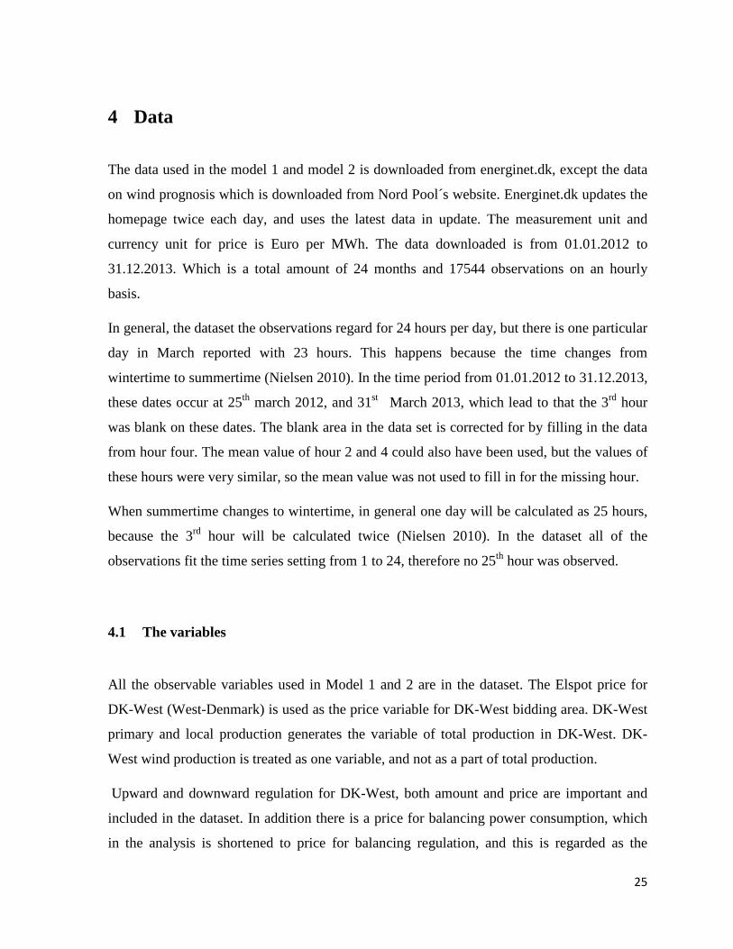
Table 2: Estimated parameters model 1.
OLS NEWEY: 24 lags NEWEY: 48 lags Dependent variable: Price of balancing regulation b/se b/se b/se Area price West Denmark 0.933*** 0.933*** 0.933*** (0.009) (0.011) (0.011) Up regulation dummy -15.295*** -15.295* -15.295* (5.042) (8.061) (8.316) Up regulation price 0.468*** 0.468** 0.468** (0.115) (0.181) (0.185) Volume traded on up regulation 0.148*** 0.148*** 0.148*** (0.009) (0.017) (0.017) Down regulation dummy 26.844*** 26.844*** 26.844*** (0.782) (1.569) (1.588) Down regulation price -0.885*** -0.885*** -0.885*** (0.020) (0.040) (0.041) Volume traded on down regulation
0.048*** 0.048*** 0.048***
(0.004) (0.006) (0.007) Constant 0.981*** 0.981*** 0.981*** (0.283) (0.367) (0.373) Number of observations N = 17544 N = 17544 N = 17544 F –Statistics R-Squared
3165.81 (0.000) 0.5990
1467.90 (0.000)
1438.33 (0.000)
***, ** and * implies significant at 1%, 5% and 10% critical levels respectively
31
The OLS, Newey (24) and Newey (48) are significant at 1 %, 5% and 10 % critical level.
The R-squared value indicate that the variation in the independent variables used to estimate
Model 1, explains approximately 60 % of the variation in the balancing price of regulation.
The two-tail p-values confirm the hypothesis that each coefficient is significantly different
from 0, at 1 %, 5 % and 10 % critical levels. The estimated coefficient spot price DK-West is
significant and with a positive sign. This indicates that the balancing market follows the
signals of the spot market. The price of balancing regulation is positively related to the spot
price, if the spot price increases the balancing price increase. This is a clear indication that
the balancing price of regulation is not independent from the spot price of DK-West. In the
table this variable is called Area price West Denmark.
The estimated dummy variable for up-regulation, which in Model 1 is given by the
coefficient 𝛽0, has a negative sign. Therefore the price of balancing regulation and the
estimated dummy variable move in the opposite direction. The results are opposite for the
down-regulation dummy variable, given by the coefficient 𝛾0, which in Model 1, which has a
positive sign. This could possibly imply stabilizing effects of the up and down regulation.
When there is up regulation power supply increases in the market, and when supply increases
the demand is closer to being satisfied, and price will eventually decrease. The same
interpretation applies for down-regulation, because when down-regulation occurs, power
supply is either withdrawn from the system or at least there is no increase in supply in the
system, which will eventually lead to a price increase. The interpreted chain of events is not
reflected as a result in one single hour of delivery, but for the interval from 12 to 36 hours of
actual delivery of power.
The estimated dummy variable for up-regulation multiplied with the area price DK-West has
a positive sign. The price of balancing regulation and this estimated variable are positively
correlated, which means that, during up-regulation an increase the area price DK- West will
imply an increase in price of balancing regulation. They are both positive and move in the
same direction when a unit change occurs. A possible explanation can be that the area price
is positively correlated with the price of balancing regulation, therefore the spot price
multiplied with the dummy variable has a positive net impact. When the down regulation
dummy is equal to 1, the dummy variable is multiplied with the spot price, and this relation
32
has a positive sign. If regulation does not occur at all, zero multiplied with the spot price, will
have no effect. The estimated dummy variable for down-regulation multiplied with the area
price of DK-West is negatively correlated to the price of balancing regulation. The estimated
coefficient is significant, but the price of balancing regulation and the coefficient move in the
opposite direction. When there is a unit decrease in the estimated coefficient, there will be an
increase in the price of balancing regulation.
The coefficient 𝛽2, which represents the dummy variable for up-regulation multiplied with
the volume of up regulation, is significant with a positive sign. This is in agreement with the
economic theory, which means that there is an increased cost. When the regulating power
volume increases, the price of balancing regulation increases, and this represents the
increased cost reflected in the increased price of balancing regulation. When regulation
volumes increase, the price for balancing regulation increases. The dummy variable picks up
the frequency of up regulation, and the volume times the frequency affects the price for
regulation. The result is almost the same for the estimated coefficient 𝛾2 , which represents
the same relation in the case of down regulation. The volume of down regulation times the
frequency of down regulation also share a positive and significant relationship with the
balancing price. The use of regulation services is regarded as an additional cost, so the
question is if it is more beneficial to use this market to minimize this cost. In the next section
the difference in average price of up-regulation and down-regulation is graphed in order to
compare the skewness and over all difference in average prices.
6.1.1 The average price of up-regulation and down-regulation
The variable price of down-regulation has a left skewed distribution, which means that the
values are mostly on the right side of the mean. The opposite is valid for the price of up-
regulation, where the distribution is right skewed. There are asymmetries in the distribution
of both variables. Figure 3 below shows average price difference of up and down regulation.
The graph representing hourly averages of up and down regulation prices is the result of eq.
(9) given in Model 1. The top graph shows the hourly average, while the graph below
33
represents the difference in hourly averages for both prices. Mean value of the up regulation
price is higher than the price for down regulation.
6.2 Results Model 2
Results from Model 2 are here represented in a similar order as was done in the analysis of
chapter five.
6.2.1 Total regulation
First, the dependable variable total regulation was generated and its distribution is shown in
the graph below. Total regulation is on the X-axis and the timeframe of 17544 hours is given
on the Y-axis. This graph represents the volume of total regulation and not price. To
510
1520
0 5 10 15 20 25Hour
(mean) price_up (mean) price_do
Daily average Up and Down regulation price
-6-4
-20
2(m
ean)
cha
nge_
pric
e
0 5 10 15 20 25Hour
Daily average price difference, Up vs Down regulation
Figure 3: Daily up and down regulation.
34
distinguish between up and down-regulation, a positive sign is given to the amount of up
regulation, and a negative sign is given to the down-regulation amount in the data set. The
bell shaped curve indicates a normal distribution, but most of the observations are around a
value of zero. The minimum value of total regulation is -704.7 and the maximum value is
714.9. The median value is zero and the mean value is 1,51 and there is a right skewed
distribution with a value of 61.58, (see Table 1). Based on the descriptive statistics most of
the values are to the right of the mean. This would imply that up-regulation dominates the
distribution, because up-regulation regard for all the positive values. However, by looking at
the graph, the most frequent value is just below zero. This value is negative and all negative
values imply that there is down-regulation. This implies a contradiction in the results. A
possible explanation can be that down-regulation happens frequently but in smaller
quantities, and the volume of up-regulation is higher each time. That in turn causes the mean
value of total regulation to become positive.
Figure 4: Distribution of the variable total regulation.
35
6.2.2 Estimated parameters Model 2
The table below provides the results of all the estimated parameters in Model 2. The
comparison of the OLS, OLS estimation with a proxy variable, and the 2SLS is done based
Findings indicate that price of using up-regulation services is higher than the price of using
down-regulation services. A higher price of up-regulation means a higher cost for producers
frequently use up-regulation services. The effects of up and down -regulation are not the
same. The possibilities of joint optimisation as discussed in chapter two and three are present.
If the price and effects of up and down regulation were the same, such possibilities would be
limited. Assume that wind power producers have a marginal cost of production close to zero
and when the market price is positive, they bid the entire amount above or equal to their
marginal cost. Then supply is bid based on the planned wind power production, which is
most likely based on the wind prognosis. The deviation between planned and actual
production can have very different consequences in the regulation market. In periods with
excessive amounts of wind, the use of the regulation market will be cheaper compared to
40
periods with little wind. This is a very clear incentive to systematically bid less supply than
the wind power prognosis on the spot market. In this manner they will need to buy down-
regulation services. These results are in line with Skytte's findings (Skytte 1999). With this
analysis it can only be stated that there is an incentive present to systematically bid on the
spot market because of the asymmetric price relation. The daily difference in average prices
of up and down-regulation are asymmetrically distributed and therefore the price difference
is of significance. The deviation between predicted and actual production of wind power
could work as an incentive to strategically place the supply bid on the spot market, and
optimize the use of regulation services. There might be a strategic incentive to systematically
bid less power supply at the spot market to obtain a reduced regulation price.
The total regulation variable has a positive mean value, and a median valued zero. However
the most frequent value was below zero according to the graph. This strengthens the
argument that a frequent use of down-regulation occurs. The amount must have been small
every time that it did not affect the mean value to become negative, and possibly every time
they up-regulate the volume has higher compared to when they down-regulate. Contradiction
between the graph and the statistics indicate that there is systematic and frequent use of
down-regulation services. To state if they strategically bid less as systematic action is
difficult to state without the additional information of the actual supply bid into Nord Pool.
The results indicate that the incentive of strategic behaviour on the spot market is present,
and therefore WtS is not equal to zero in equation (2) and planned wind power production is
determined by wind power production supply bids and the strategic element related to wind
power.
Ideally, planned wind power production and actual wind power production would be the
same, and there would not be any systematic use of the regulation market. Thus wind power
prognosis would have been 100 % accurate and no deviations would have taken place. In
reality this is very challenging to obtain.
When Model 2 was estimated the assumption was that actual wind power production is an
exogenous independent variable in predicting total regulation. As seen from specification
tests results, wind power production variable included in the OLS produced biased results
due to possible missing variables or measurement error problem. Then planned wind power
41
production, wind power prognosis is used as a proxy variable alongside actual wind power
production when the OLS was estimated again. Now results were noticeably different
compared to the OLS without a proxy but the specification tests did not improve
substantially. The results from instrument variable 2SLS estimation indicate wind power
production to be endogenous in predicting total regulation. There is a very strong indication
of measurement error in the model. Significant measurement error could be indirect evidence
on systematic action of strategic behaviour. The findings imply that the incentive to act
strategically is present, and in addition to that finding there is an unforeseen measurement
error in the model.
On the basis of the results from Model 2, one may significant systematic unforeseen
behaviour. The regulation market and the spot market are supposed to be treated as two
separate markets. Systematic use of the regulation market may encourage gaming strategies,
and collusion among the wind power producers.
However, there are several limitations in the provided analysis. No cross validation has been
done and hence these findings are only valid for these 24 months. The models are not
validated outside the sample. The analysis for the long -run may produce completely
different results. Another limitation is that this analysis is based on indirect evidence. If there
was data available on the actual bidding amount submitted to Nord Pool, this analysis may
possibly show different results. An analysis done directly using actual bidding data may lead
to different results, as there would be direct evidence for the findings. The chain of events in
the energy market are very strongly linked to each other, meaning that there may be factors
present which have not been considered in the analyssi, such as consumer aspect, seasonal
variation in demand, and the retailers role all together. This research focused only on the
production side of the market, which may not be a complete picture. One important thing in
this respect is that the regulation market is not only used by wind power producers, while the
in the analysis there is an assumption that conventional power producers can control their
production. In reality, wind power producers in often struggle with anticipating their actual
production amount.
In the event that Denmark decides to pursue its plans of increasing its wind power
production, several aspects of this analysis may be relevant. The cost structure of wind power
42
producers must be taken into consideration when more actors will enter the market. The
interests of Nord Pool, the regulation market and the wind power producers must be taken
into consideration when dealing with increased wind power in the system. In addition large
investments are required to expand the wind power sector. The investment plans bring
forward higher uncertainty and in addition to that if the strategic use of the regulation market
adds up as a factor of economic inefficiency the plans must be evaluated very carefully.
To sum up, the findings in Model 1 rejected the first hypothesis, because there is a difference
in price for up-and down regulation, and the use of the regulation market is asymmetric. The
findings in Model 2 rejected the second hypothesis, and wind power production is an
endogenous variable when predicting the total regulation amount. The deviation between
planned and actual production of wind power can be used as an incentive to place the supply
bids strategically on the spot market, to obtain a better price in the regulation market. This
behaviour distinguishes from mark-up and capital-withdrawal strategies as discussed in
chapter 2.3.1. The effect using the regulation market strategically may not have a direct
effect on the demand and thus may not affect consumers at all. Whether this type of incentive
leads to economic inefficiency or not, cannot be stated without collecting substantial
evidence and data for the long run.
43
This page intentionally left blank.
44
7 Conclusions
The objective of this study was to test for systematic relationship between up and down-
regulation and price for regulating power. Results imply that the deviation between predicted
production and actual production of wind power could work as an incentive to strategically
submit supply bid at the spot market, and optimize the use of regulation services because of
the higher cost of up-regulation compared to down-regulation. This incentive can lead the
producers to place a bid lower than the actual production, to avoid the use of up-regulation
services. In addition the results also implied that there was a frequent use of down-regulation
services even if the mean value of the observations was positive, and related to up-regulation.
Since the spot price effect the total regulation price, the cost of regulation can be anticipated
before the actual delivery of power. The second analysis concluded that wind power
production was endogenous in predicting total regulation and the instrument of wind
prognosis did not correct for endogeneity. Actual wind power production should be equal to
planned wind power production and therefore be exogenous in predicting total regulation. An
unobservable strategic element may have been added to the supply bid and comes up in the
model as a systematic measurement error.
For further research it is recommended to analyse whether strategic bidding behaviour will
lead to externalities associated with wind power production in the future. If it turns out that
strategic use of the regulation market is revealed in the long run, then some improved bidding
structure should be suggested for producers of wind power that will decrease the
opportunities to use the regulation market strategically.
45
References
Danish Wind Industry Association. (2014). WIND ENERGY: Denmark DK. Available at: http://denmark.dk/en/green-living/wind-energy/ (accessed: April 20).
Dr. Petrov, D. K., Dr. Scarsi, G. C. & van der Veem, W. (2003). Modelling Strategic Bidding Behavior In Power Markets. Eropean Electricity Markets (September 2003).
Energinett.DK. (2014). Available at: https://www.energinet.dk/EN/Sider/default.aspx. Forbes, K. F., Stampini, M. & Zampelli, E. M. (2007). Wind Power and the Electricity Market for
Upward Regulation: Evidence for Western Denmark. USAEE. Green, H. W. (1990). Econometric Analysis. Second ed.: Macmillan Publishing Company. Jensen, T. K. & Sørensen, R. Z. (2014). Facts and numbers: Danish Energy Agency. Available at:
Kanter, J. (2012, January 22, 2012). Obstacles to Danish Wind Power. The New York Times. Lentz, A. H. & Strandmark, L. (2014). Danish Climate and Energy Policy: Danish Energy Agency.
Available at: http://www.ens.dk/en/policy/danish-climate-energy-policy (accessed: April 10).
Nielsen, B. (2010). Introduktion til udtræk af markedsdata: Energinet.DK. Nord Pool. (2014a). The Nordic Electricity Exchange and The Nordic Model for a Liberalized
Electricity Market. 19 (accessed: 20.01.2014). Nord Pool. (2014b). Price Formation in Nord Pool Spot: Nord Pool. Available at:
NordPool. (2013). History: Nord Pool Spot. Available at: http://www.nordpoolspot.com/About-us/History/ (accessed: April 15).
Reichstein, T. (2011). Econometrics Endogeneity: Department of Innovation and Organizational Economics Copenhagen Business School. 45 pp.
Skytte, K. (1999). The regulating power market on the Nordic power exchange Nord Pool: an econometric analysis. Energy Economics, 21: 14.
Young, D. (2014). Chapter 13: Measurement Errors and Instrumental Variables Regression: Pennsylvania State University Available at: https://onlinecourses.science.psu.edu/stat501/node/200 (accessed: March 2014).
Area price Denmark West -22.877*** 0.000 24 Up regulation price -33.833*** 0.000 7 Volume traded up regulation -31.081*** 0.000 5 Down regulation price -32.623*** 0.000 10 Volume traded on down regulation -38.495*** 5
Chi-square/p-value Chi-square/p-value White´s test 327.22*** 511.56*** (0.000) (0.000) Breusch-Pagan 144.18*** 0.89 (0.000) (0.347) Link test T-statistic /P-value T-statistic /P-value Predicted hat 20.52*** 37.24*** (0.000) (0.000) Predicted hat squared -7.39*** -4.16*** (0.000) (0.000) Likelihood ratio test comparing OLS and OLS with proxy LR Chi-square/p-value 1002.19*** (0.000) Conclusion There is a significant difference
Test for endogneity Durbin Chi-square (1)/p-value 974.098*** (0.000) Wu-Hausman F-statistic(1,17539)/P-value 1031.07 (0.000) Conclusion Wind production is endogenous
C
Test for suitability of wind prognosis, net exports and total production as good instruments for wind production


![Danish Wind Power Academy 2016 - Vestas training / Siemens ... Presentation 2016 GB.pdf · [Module index END] Page Technical training for the wind turbine industry DWPA Presentation](https://static.documents.pub/doc/80x56/5dd09866d6be591ccb61c111/danish-wind-power-academy-2016-vestas-training-siemens-presentation-2016.jpg)

