AN ANALYSIS OF BLASIUS BOUNDARY LAYER SOLUTION WITH DIFFERENT NUMERICAL METHODS MUSTAFA SAIFUDEEN BIN ABDUL WALID Report submitted in partial fulfillment of the requirement for the award of Bachelor of Mechanical Engineering Faculty of Mechanical Engineering UNIVERSITI MALAYSIA PAHANG JUNE 2012
Transcript
AN ANALYSIS OF BLASIUS BOUNDARY LAYER SOLUTION
WITH DIFFERENT NUMERICAL METHODS
MUSTAFA SAIFUDEEN BIN ABDUL WALID
Report submitted in partial fulfillment of the requirement
for the award of Bachelor of Mechanical Engineering
Faculty of Mechanical Engineering
UNIVERSITI MALAYSIA PAHANG
JUNE 2012
vii
ABSTRACT
The nonlinear equation from Prandtl has been solved by Blasius using Fourth order
Runge-Kutta methods. The thesis aims to study the effect of solving the nonlinear
equation using different numerical methods. Upon the study of the different numerical
methods be use to solve the nonlinear equation, the Predictor-Corrector methods, the
Shooting method and the Modified Predictor-Corrector method were used. The
differences of the methods with the existing Blasius solution method were analyzed.
The Modified Predictor-Corrector method was developed from the Predictor-Corrector
method by adjusting the pattern of the equation. It shows the graphs of the , and against the eta. All the methods have the same shape of graph. The Shooting method is
closely to the Blasius method but not stable at certain value. The Variational Iteration
method that has been used cannot be proceeding because the method only valid for the
earlier flows and lost the pattern at the higher value of eta. It can be comprehend that the
Predictor-Corrector methods, the Shooting method and the Modified Predictor-
Corrector method achieve the conditions and can be applied to solve the nonlinear
equation with minimal differences. The methods are highly recommended to solve the
Sakiadis problem instead of the stationary flat plate problem.
viii
ABSTRAK
Persamaan tidak linear daripada Prandtl telah diselesaikan oleh Blasius dengan
menggunakan kaedah penyelesaian Runge-Kutta keempat. Kaedah penyelesaian
persamaan tidak linear tersebut dikaji melalui penggunaan kaedah penyelesaian
berangka yang berbeza di dalam tesis ini. Kaedah Peramal-Pembetul, Kaedah
Tembakan dan juga Kaedah Ubahan Peramal-Pembetul telah digunakan. Perbezaan
kaedah-kaedah ini dengan kaedah yang sedia ada Blasius di analisis. Kaedah Ubahan
Peramal-Pembetul telah dikeluarkan daripada kaedah asal Peramal-Pembetul dengan
melaraskan corak persamaannya. Ia menunjukkan graf , dan terhadap eta. Semua
kaedah mempunyai bentuk graf yang sama dengan kaedah penyelesaian Blasius.
Kaedah Tembakan adalah paling hampir dengan kaedah penyelesaian Blasius namun
terdapat sedikit ketidakstabilan pada titik-titik tertentu. Kaedah Lelaran Perubahan pula
telah digunakan namun tidak dapat diteruskan kerana kaedah ini hanya sah pada aliran
permulaan sahaja dan hilang corak pada nilai eta yang lebih tinggi. Kaedah Peramal-
Pembetul, Kaedah Tembakan dan juga Kaedah Ubahan Peramal-Pembetul mencapai
syarat-syarat dan boleh digunakan untuk menyelesaikan persamaan tidak linear dengan
perbezaan yang kecil. Kaedah-kaedah ini amat disyorkan untuk menyelesaikan masalah
Sakiadis iaitu plat rata yang tidak statik.
ix
TABLE OF CONTENTS
Page
EXAMINER’S DECLARATION ii
SUPERVISOR’S DECLARATION iii
STUDENT’S DECLARATION iv
DEDICATION v
ACKNOWLEDGEMENTS vi
ABSTRACT vii
ABSTRAK viii
TABLE OF CONTENTS ix
LIST OF TABLES xi
LIST OF FIGURES xii
CHAPTER 1 INTRODUCTION
1.1 Project Background 1
1.2 Problem Statement 1
1.3 Objective 1
1.4 Scope 2
1.5 Flow Chart 2
CHAPTER 2 LITERATURE REVIEW
2.1 Introduction 4
2.2 History
2.2.1 Sir Ludwig Prandtl 4
2.2.2 Blasius 6
2.2.3 Navier-Stokes Equation 7
2.3 Boundary Layer 8
2.4 Continuity Equation 9
2.5 Momentum Equation 10
2.6 Numerical Methods 10
2.7 Derivation of Boundary Layer Equation 11
x
CHAPTER 3 METHODOLOGY
3.1 Introduction 14
3.2 Methodology Flow Chart 14
3.3 Literature Study 16
3.4 Blasius Solution’s Table (Controlled Data) 16
3.5 Predictor-Corrector Method 16
3.6 Shooting Method with Maple 18
3.6.1 Iteration of using Shooting Method 19
3.7 Predictor-Corrector Method with Central Difference 20
3.8 Variational Iteration Method 21
3.9 Usage of Microsoft Excel Software 24
CHAPTER 4 RESULT AND DISCUSSION
4.1 Shooting Methods with Maple 25
4.2 Comparison of the Graphs between Predictor-Corrector Method,
Shooting Method and Modified Predictor-Corrector Method 26
4.2.1 Calculating the Error Percentage 27
4.2.2 Error Percentage of with the Other Methods to the
Blasius Solution Method 28
4.2.3 Comparison between the Three Methods 29
4.2.4 Error Percentage of with the Other Methods to the
Blasius Solution Method 30
4.2.5 Error Percentage of With the Other Methods to the
Blasius Solution Method 31
4.3 Comparison of the Graph Obtain in Maple 32
4.4 Variational Iteration Method Result 33
CHAPTER 5 CONCLUSION AND RECOMMENDATIONS
5.1 Conclusion 34
5.2 Recommendations 35
REFERENCES 36
APPENDICES 38
xi
LIST OF TABLES
Table No. Page
2.1 Prandtl’s chronology 5
2.2 Blasius’s chronology 6
3.1 Result of Blasius solution using 4th
order Runge-Kutta methods 16
4.1 Iteration of Using Shooting Methods with Maple 25
4.2 Comparison Result of 27
xii
LIST OF FIGURES
Figure No. Page
1.1 Project flow chart 3
2.1 Ludwig Prandtl 5
2.2 Blasius 6
2.3 Laminar boundary layer along a flat plate 8
3.1 Methodology flow chart 15
3.2 Asymptotic graph comparison 20
4.1 Graph of , and VS eta (Predictor-Corrector) 26
4.2 Graph of , and VS eta (Shooting) 26
4.3 Graph of , and VS eta (Modified Predictor-Corrector) 26
4.4 Error Percentage of of Other Methods towards Blasius Solution 28
4.5 Error Percentage of of Other Methods towards Blasius Solution
(Maximum Value)
29
4.6 Error Percentage of with other methods to the Blasius Solution 30
4.7 Error Percentage of with other methods to the Blasius Solution 31
4.8 Comparison Graph of against 32
4.9 Graph of against eta using Variational Iteration Method 33
CHAPTER 1
INTRODUCTION
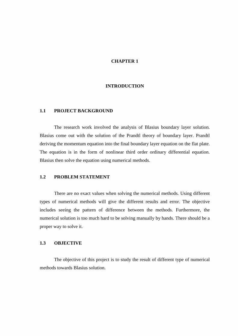
1.1 PROJECT BACKGROUND
The research work involved the analysis of Blasius boundary layer solution.
Blasius come out with the solution of the Prandtl theory of boundary layer. Prandtl
deriving the momentum equation into the final boundary layer equation on the flat plate.
The equation is in the form of nonlinear third order ordinary differential equation.
Blasius then solve the equation using numerical methods.
1.2 PROBLEM STATEMENT
There are no exact values when solving the numerical methods. Using different
types of numerical methods will give the different results and error. The objective
includes seeing the pattern of difference between the methods. Furthermore, the
numerical solution is too much hard to be solving manually by hands. There should be a
proper way to solve it.
1.3 OBJECTIVE
The objective of this project is to study the result of different type of numerical
methods towards Blasius solution.
2
1.4 SCOPE
The project scope is firstly to know briefly about the boundary layer theory and
how the boundary layer happened. The boundary layer that formed allowed us to
determine the values that related; as example temperature, pressure and etc. Hence, the
theory that comes out from Prandtl later being solved by the Blasius to be derived and
proved with numerical methods. Once the methods proven, there should be a proper
way proposed to solve the equation usually using software; as example Fortran, C++ or
MATLAB.
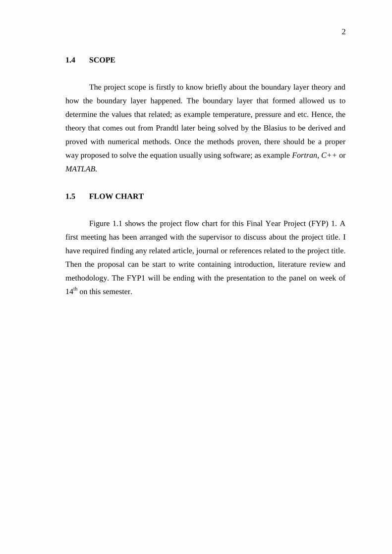
1.5 FLOW CHART
Figure 1.1 shows the project flow chart for this Final Year Project (FYP) 1. A
first meeting has been arranged with the supervisor to discuss about the project title. I
have required finding any related article, journal or references related to the project title.
Then the proposal can be start to write containing introduction, literature review and
methodology. The FYP1 will be ending with the presentation to the panel on week of
14th
on this semester.
3
Figure 1.1: Project Flow Chart
CHAPTER 2
LITERATURE REVIEW
2.1 INTRODUCTION
The literature review consists of the brief explanations of elements that related to
this project. The analysis of Blasius boundary layer solution is related to the boundary
layer theory and also boundary layer equation. The research of the boundary layer was
done by the German scientist, Ludwig Prandtl with his presented benchmark paper on
boundary layer in 1904 (Prandtl 1904). Later, solution of the boundary layer theory was
done by his student, Blasius. In solving the boundary layer theory, several
approximation that eliminate terms reducing the Navier-Stokes equation to a simplified
form that is more easily solvable.
The mathematical parts of this project include the numerical methods. There are
quite a number of numerical methods to solve the differential equation. As the boundary
layer equation is in third order ordinary differential equation, the numerical method
such as Runge-Kutta, Euler and also Predictor-Corrector methods are the available
method that solve the problem. These elements will be briefly discussed in the further
part of this chapter.
2.2 HISTORY
2.2.1 Sir Ludwig Prandtl
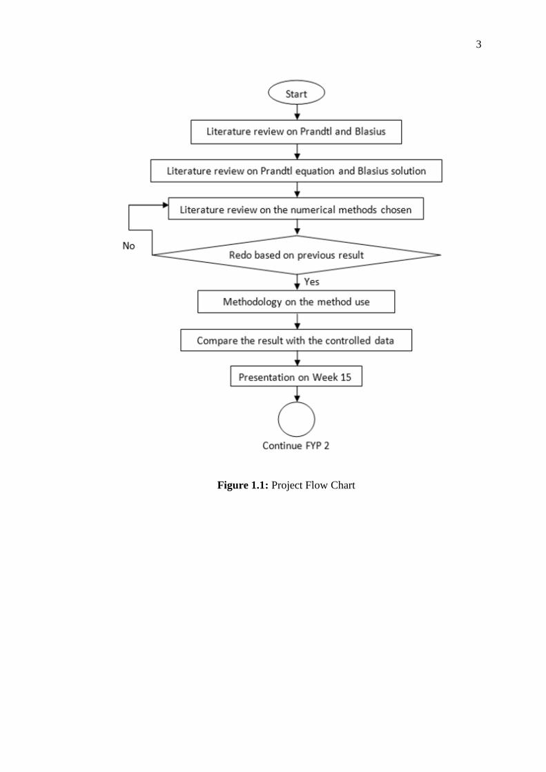
Sir Ludwig Prandtl was born in Freising, Bavaria (Beyond the Boundary Layer
Concept). His father, Alexander Prandtl, was a professor of surveying engineering at
5
The Agricultural College at Weihenstephen, near Freising. The Prandtls had three
children, but two died at birth and Ludwig grew up as an only child. His mother
suffered from a protracted illness, Ludwig became very close to his father. He became
interested in his father’s books on physics, machinery and instruments at an early age.
Figure 2.1: Ludwig Prandtl
(Source:Anderson, 2005)
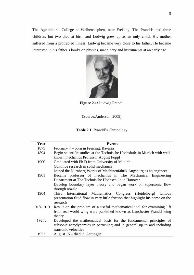
Table 2.1: Prandtl’s Chronology
Year Events
1875 February 4 – born in Freising, Bavaria
1894 Begin scientific studies at the Technische Hochshule in Munich with well-
known mechanics Professor August Foppl
1900 Graduated with Ph.D from University of Munich
Continue research in solid mechanics
Joined the Nurnberg Works of Machinenfabrik Augsburg as an engineer
1901 Became professor of mechanics in The Mechanical Engineering
Department at The Technische Hochschule in Hanover
Develop boundary layer theory and began work on supersonic flow
through nozzle
1904 Third International Mathematics Congress (Heidelberg) famous
presentation fluid flow in very little friction that highlight his name on the
research
1918-1919 Result on the problem of a useful mathematical tool for examining lift
from real world wing were published known as Lanchester-Prandtl wing
theory
1920s Developed the mathematical basis for the fundamental principles of
subsonic aerodynamics in particular; and in general up to and including
transonic velocities
1953 August 15 – died in Gottingen
6
He spent the remainder of his life to become director of the institute for technical
physics in the prestigious University of Gottingen and built his laboratory into the
greatest aerodynamics research center in early 20th
century.
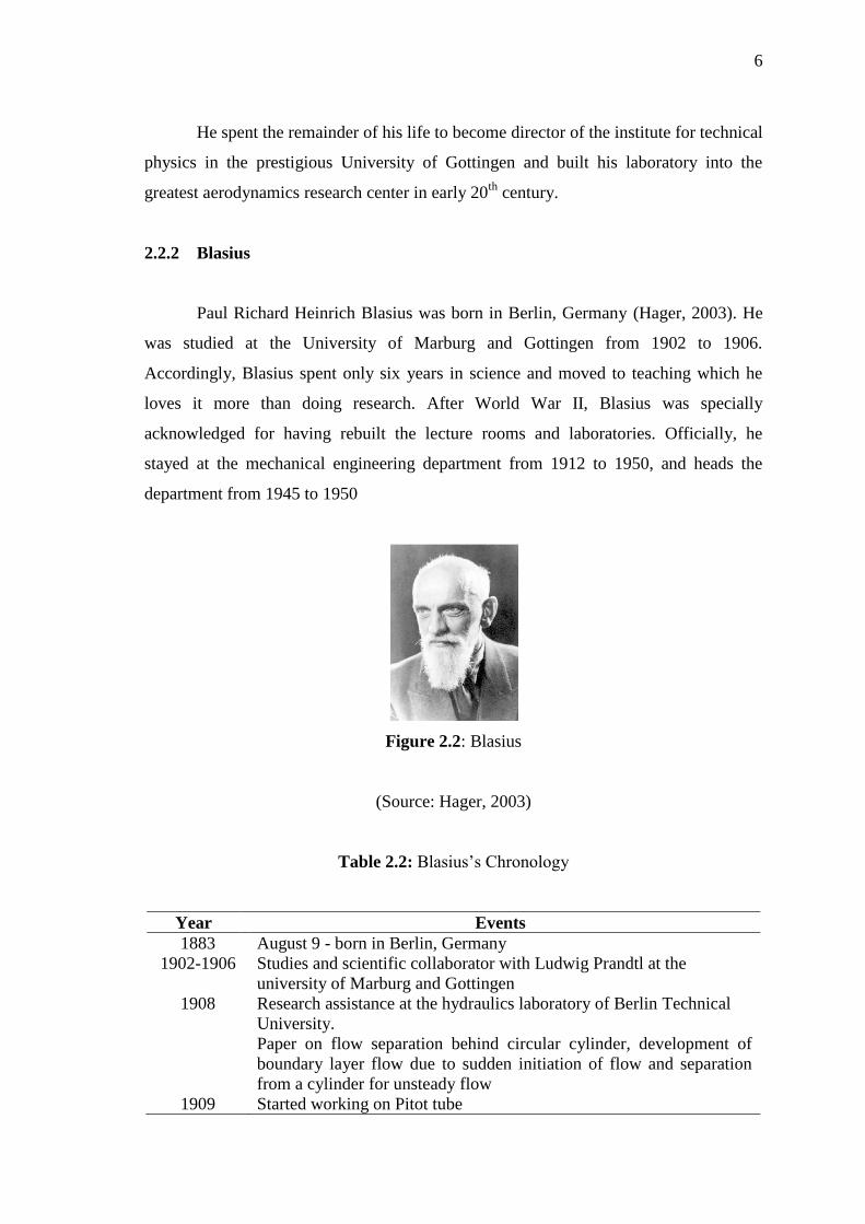
2.2.2 Blasius
Paul Richard Heinrich Blasius was born in Berlin, Germany (Hager, 2003). He
was studied at the University of Marburg and Gottingen from 1902 to 1906.
Accordingly, Blasius spent only six years in science and moved to teaching which he
loves it more than doing research. After World War II, Blasius was specially
acknowledged for having rebuilt the lecture rooms and laboratories. Officially, he
stayed at the mechanical engineering department from 1912 to 1950, and heads the
department from 1945 to 1950
Figure 2.2: Blasius
(Source: Hager, 2003)
Table 2.2: Blasius’s Chronology
Year Events
1883 August 9 - born in Berlin, Germany
1902-1906 Studies and scientific collaborator with Ludwig Prandtl at the
university of Marburg and Gottingen
1908 Research assistance at the hydraulics laboratory of Berlin Technical
University.
Paper on flow separation behind circular cylinder, development of
boundary layer flow due to sudden initiation of flow and separation
from a cylinder for unsteady flow
1909 Started working on Pitot tube
7
Table 2.2: Continue
Year Events
1910 Second key paper- classical potential theory applied; (i)force the
exerted body immersed in a fluid flow; (ii)potential flow over weirs
1911 Investigated the curve airfoil using the Kutta method.
Blasius reconsider mathematical methods applied to potential flow and
derived an expression for the force of an obstacle positioned in a
stream.
1912 Publish relating friction coefficient of turbulent smooth pipe flow.
First to derive a law relating to so-called turbulent smooth pipe flows.
Teacher at The Technical College Of Hamburg
1931 Undergraduate books on heat transfer
1934 Undergraduate book on mechanics
1912-1950 Continued lecturing in Hamburg
1970 April 24 – passed away in Hamburg
2.2.3 Navier-Stokes Equation
The traditional model of fluids used in physics is based on a set of partial
differential equations known as the Navier-Stokes equations. These equations were
originally derived in the 1840s on the basis of conservation laws and first-order
approximations. For very low Reynolds numbers and simple geometries, it is often
possible to find explicit formulas for solutions to the Navier-Stokes equations. But even
in the regime of flow where regular arrays of eddies are produced, analytical methods
have never yielded complete explicit solutions. In this regime, however, numerical
approximations are fairly easy to find.
The ability of computers has been capable enough to allow computations at least
nominally to be extended to acceptably higher Reynolds numbers since about the 1960s.
And indeed it has become increasingly common to see numerical results given far into
the turbulent region that leading sometimes to the assumption that turbulence has
somehow been derived from the Navier-Stokes equations. But just what such numerical
results actually have to do with detailed solutions to the Navier-Stokes equations is not
clear. For in particular it ends up being almost impossible to distinguish whatever
genuine instability and apparent randomness may be implied by the Navier-Stokes
equations from artifacts that get introduced through the discretization procedure used in
solving the equations on a computer. At a mathematical level analysis of the Navier-
8
Stokes has never established the formal uniqueness and existence of solutions. Indeed,
there is even some evidence that singularities might almost inevitably form, which
would imply a breakdown of the equations.
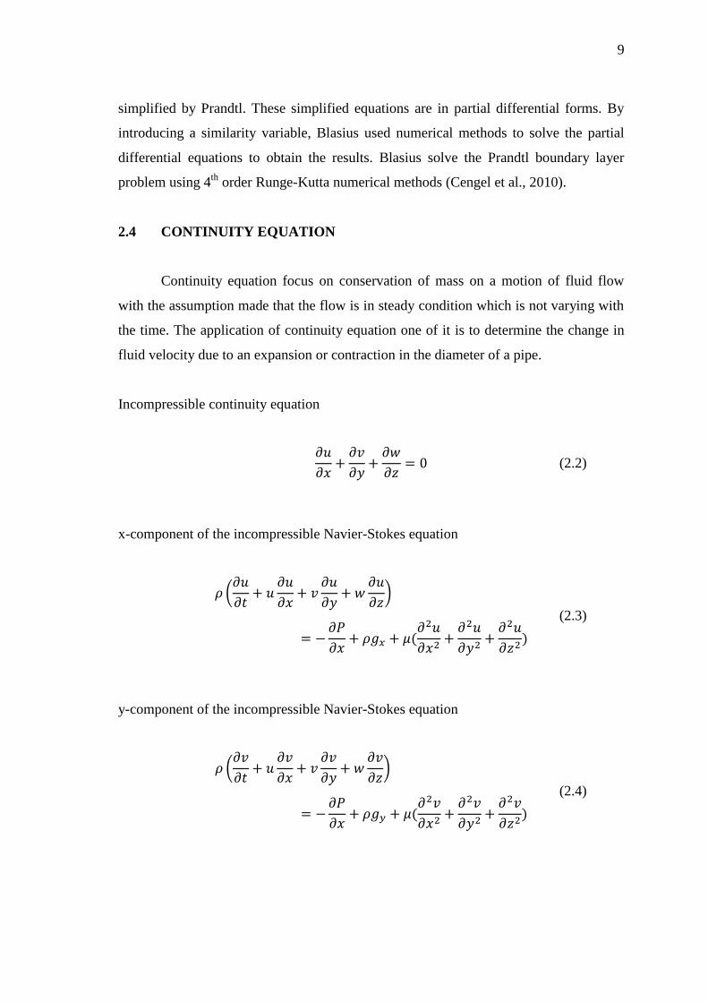
The Navier-Stokes equation of incompressible flow of Newtonian fluid with
constant properties
(2.1)
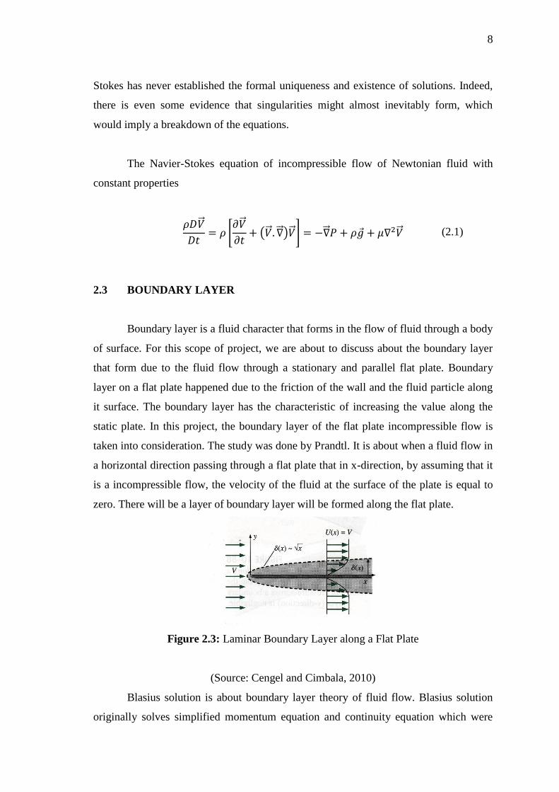
2.3 BOUNDARY LAYER
Boundary layer is a fluid character that forms in the flow of fluid through a body
of surface. For this scope of project, we are about to discuss about the boundary layer
that form due to the fluid flow through a stationary and parallel flat plate. Boundary
layer on a flat plate happened due to the friction of the wall and the fluid particle along
it surface. The boundary layer has the characteristic of increasing the value along the
static plate. In this project, the boundary layer of the flat plate incompressible flow is
taken into consideration. The study was done by Prandtl. It is about when a fluid flow in
a horizontal direction passing through a flat plate that in x-direction, by assuming that it
is a incompressible flow, the velocity of the fluid at the surface of the plate is equal to
zero. There will be a layer of boundary layer will be formed along the flat plate.
Figure 2.3: Laminar Boundary Layer along a Flat Plate
(Source: Cengel and Cimbala, 2010)
Blasius solution is about boundary layer theory of fluid flow. Blasius solution
originally solves simplified momentum equation and continuity equation which were
9
simplified by Prandtl. These simplified equations are in partial differential forms. By
introducing a similarity variable, Blasius used numerical methods to solve the partial
differential equations to obtain the results. Blasius solve the Prandtl boundary layer
problem using 4th
order Runge-Kutta numerical methods (Cengel et al., 2010).
2.4 CONTINUITY EQUATION
Continuity equation focus on conservation of mass on a motion of fluid flow
with the assumption made that the flow is in steady condition which is not varying with
the time. The application of continuity equation one of it is to determine the change in
fluid velocity due to an expansion or contraction in the diameter of a pipe.
Incompressible continuity equation
(2.2)
x-component of the incompressible Navier-Stokes equation
(2.3)
y-component of the incompressible Navier-Stokes equation
(2.4)
10
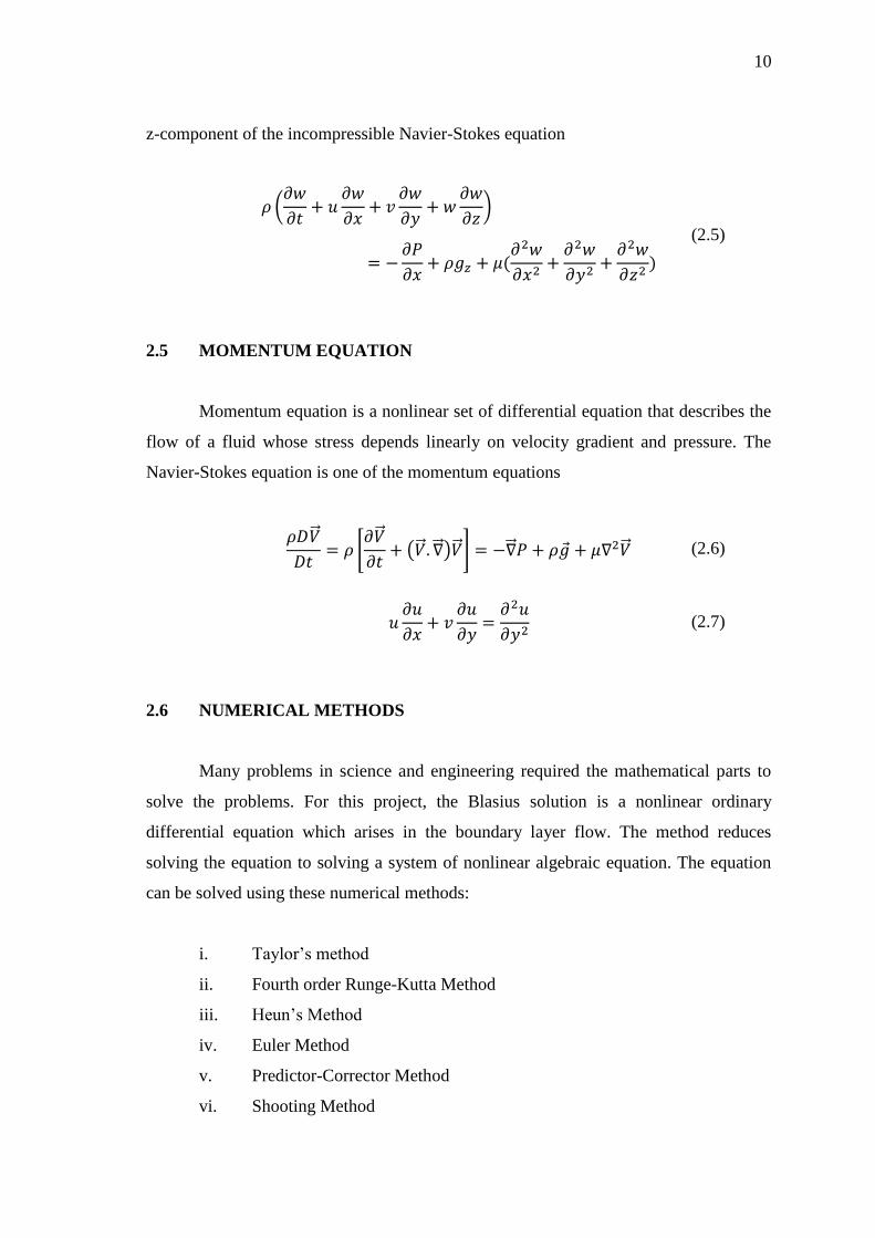
z-component of the incompressible Navier-Stokes equation
(2.5)
2.5 MOMENTUM EQUATION
Momentum equation is a nonlinear set of differential equation that describes the
flow of a fluid whose stress depends linearly on velocity gradient and pressure. The
Navier-Stokes equation is one of the momentum equations
(2.6)
(2.7)
2.6 NUMERICAL METHODS
Many problems in science and engineering required the mathematical parts to
solve the problems. For this project, the Blasius solution is a nonlinear ordinary
differential equation which arises in the boundary layer flow. The method reduces
solving the equation to solving a system of nonlinear algebraic equation. The equation
can be solved using these numerical methods:
i. Taylor’s method
ii. Fourth order Runge-Kutta Method
iii. Heun’s Method
iv. Euler Method
v. Predictor-Corrector Method
vi. Shooting Method
11
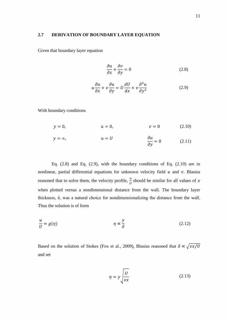
2.7 DERIVATION OF BOUNDARY LAYER EQUATION
Given that boundary layer equation
(2.8)
(2.9)
With boundary conditions
(2.10)
(2.11)
Eq. (2.8) and Eq. (2.9), with the boundary conditions of Eq. (2.10) are in
nonlinear, partial differential equations for unknown velocity field and . Blasius
reasoned that to solve them, the velocity profile,
should be similar for all values of
when plotted versus a nondimensional distance from the wall. The boundary layer
thickness, δ, was a natural choice for nondimensionalizing the distance from the wall.
Thus the solution is of form
(2.12)
Based on the solution of Stokes (Fox et al., 2009), Blasius reasoned that
and set
(2.13)
12
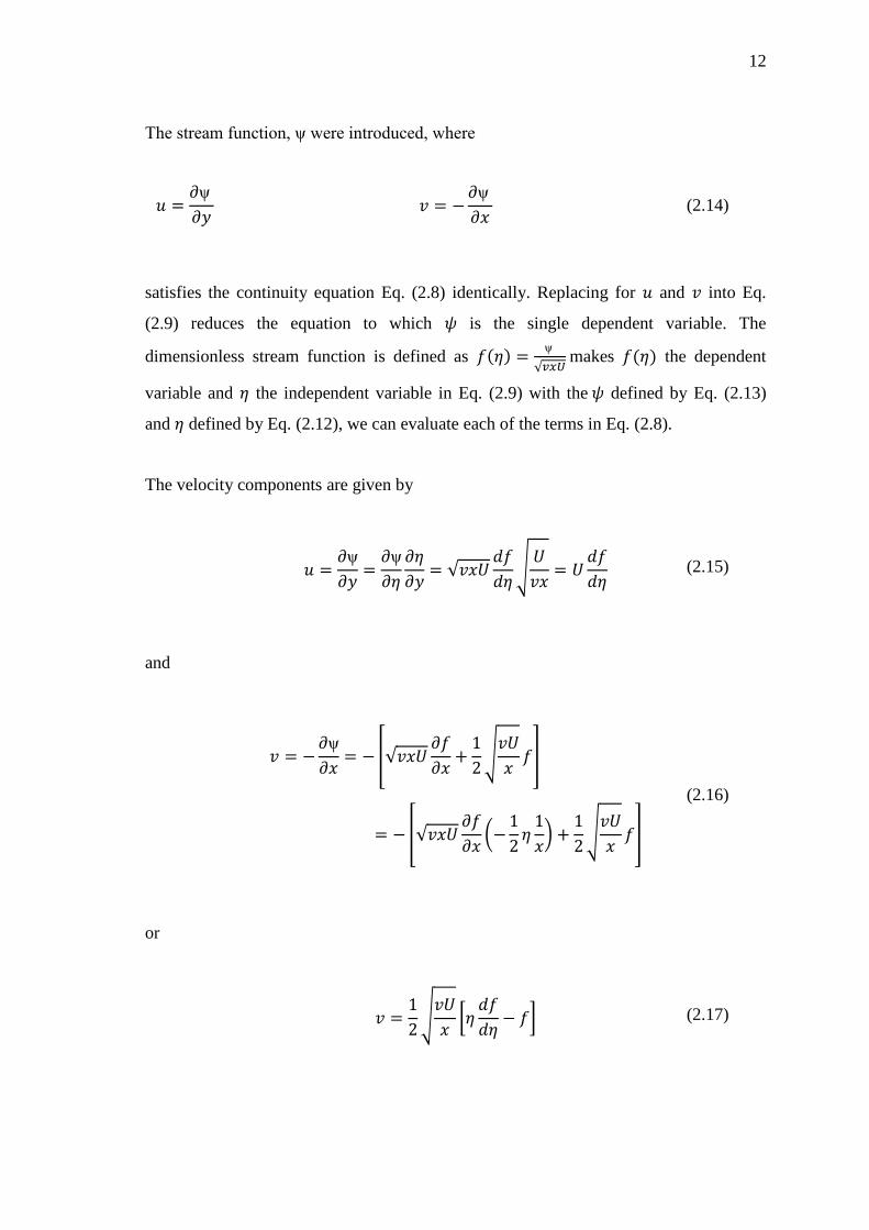
The stream function, ψ were introduced, where
ψ
ψ
(2.14)
satisfies the continuity equation Eq. (2.8) identically. Replacing for and into Eq.
(2.9) reduces the equation to which is the single dependent variable. The
dimensionless stream function is defined as ψ
makes the dependent
variable and the independent variable in Eq. (2.9) with the defined by Eq. (2.13)
and defined by Eq. (2.12), we can evaluate each of the terms in Eq. (2.8).
The velocity components are given by
ψ
ψ
(2.15)
and
or
(2.17)
ψ
(2.16)
13
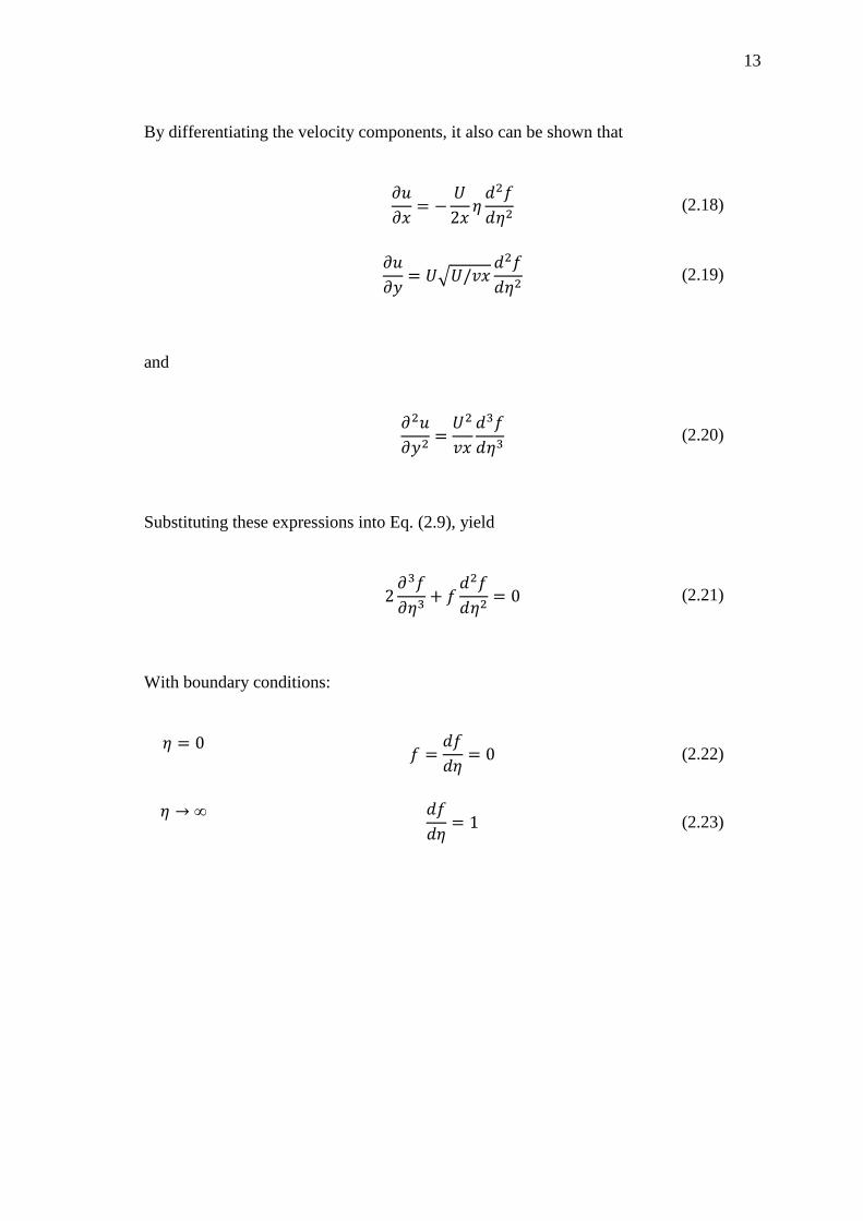
By differentiating the velocity components, it also can be shown that
(2.18)
(2.19)
and
(2.20)
Substituting these expressions into Eq. (2.9), yield
(2.21)
With boundary conditions:
(2.22)
(2.23)
CHAPTER 3
METHODOLOGY
3.1 INTRODUCTION
This chapter is focusing on explaining clearly the steps taken to complete the
project in order to obtain the result and discussion. The procedure must be done
systematically to make sure there is no mistake and conflict on the result obtain. A good
methodology can describe the project flow smoothly and the project framework that
contains the process element hence it becomes the guideline to find the objective
required.
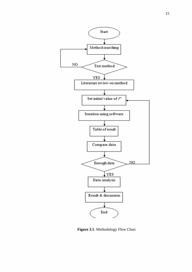
3.2 METHODOLOGY FLOW CHART
The planning is very important to give an illustration about the project flow
process to make sure the progress project is satisfied with the time required. The flow
chart can describes the project flow and process briefly. Hence the project will run
smoothly as scheduled. This methodology will show the sequence of the project flow
including in method choosing, literature review on related methods, and data analysis
and discussion on the result obtained.
15
Figure 3.1: Methodology Flow Chart
16
3.3 LITERATURE STUDY
In order to give a more understanding based on project title a research journal,
conference article, reference book and others are used as reference. The main term like
boundary layer and Blasius solution are the key to the related article found. Based on
the article found, it is important to know the process of method of solving equation used
until the data table was gathered.
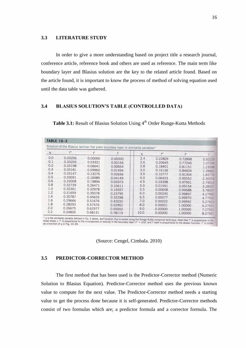
3.4 BLASIUS SOLUTION’S TABLE (CONTROLLED DATA)
Table 3.1: Result of Blasius Solution Using 4th
Order Runge-Kutta Methods
(Source: Cengel, Cimbala. 2010)
3.5 PREDICTOR-CORRECTOR METHOD
The first method that has been used is the Predictor-Corrector method (Numeric
Solution to Blasius Equation). Predictor-Corrector method uses the previous known
value to compute for the next value. The Predictor-Corrector method needs a starting
value to get the process done because it is self-generated. Predictor-Corrector methods
consist of two formulas which are; a predictor formula and a corrector formula. The
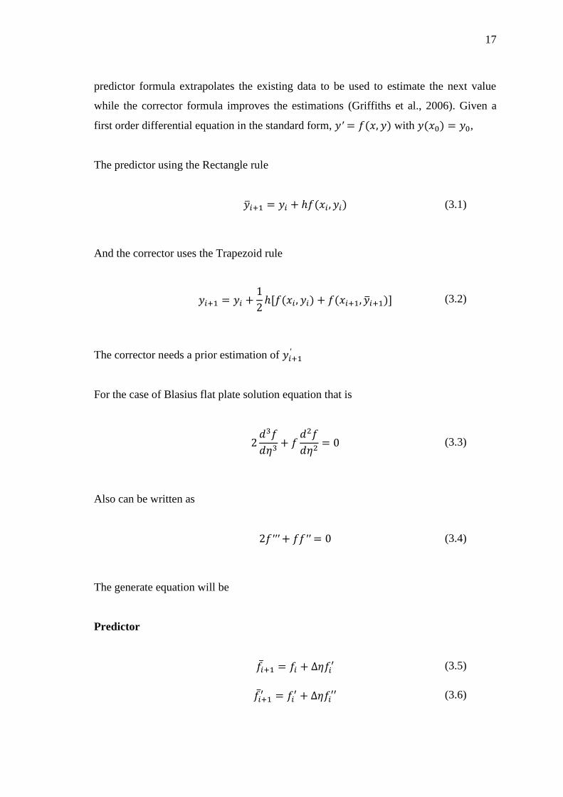
17
predictor formula extrapolates the existing data to be used to estimate the next value
while the corrector formula improves the estimations (Griffiths et al., 2006). Given a
first order differential equation in the standard form, with ,
The predictor using the Rectangle rule
(3.1)
And the corrector uses the Trapezoid rule
(3.2)
The corrector needs a prior estimation of
For the case of Blasius flat plate solution equation that is