Fichera, Eleonora (2010) An analysis of households' credit markets in Ethiopia and Malawi. PhD thesis, University of Nottingham. Access from the University of Nottingham repository: http://eprints.nottingham.ac.uk/11373/1/Thesis.pdf Copyright and reuse: The Nottingham ePrints service makes this work by researchers of the University of Nottingham available open access under the following conditions. This article is made available under the University of Nottingham End User licence and may be reused according to the conditions of the licence. For more details see: http://eprints.nottingham.ac.uk/end_user_agreement.pdf For more information, please contact [email protected]
Transcript
Fichera, Eleonora (2010) An analysis of households' credit markets in Ethiopia and Malawi. PhD thesis, University of Nottingham.
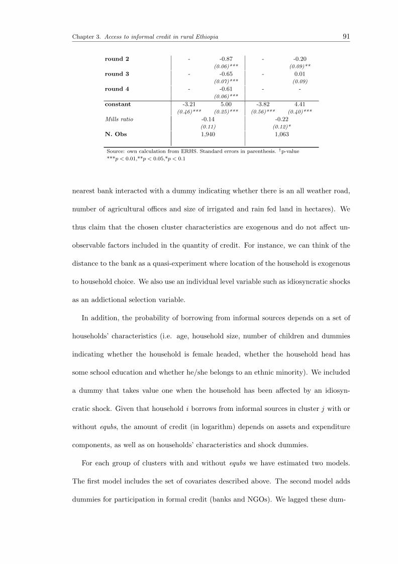
Access from the University of Nottingham repository: http://eprints.nottingham.ac.uk/11373/1/Thesis.pdf
Copyright and reuse:
The Nottingham ePrints service makes this work by researchers of the University of Nottingham available open access under the following conditions.
This article is made available under the University of Nottingham End User licence and may be reused according to the conditions of the licence. For more details see: http://eprints.nottingham.ac.uk/end_user_agreement.pdf
ATE Average Treatment EffectATT Average Treatment effect on TreatedCBM Commercial Bank of MalawiCIA Conditional Independence AssumptionCM Conditional MomentERHS Ethiopian Rural Household SurveyEUHS Ethiopian Urban Household SurveyFIML Full Information Maximum LikelihoodFMHFS Financial Markets and Household Food SecurityGTZ German agency for Technical CooperationHWS Huber White SandwichIFAD International Fund for Agricultural DevelopmentIFPRI International Food Policy Research InstituteIIA Independence of Irrelevant AlternativesIV Instrumental VariableLAD Least Absolute DeviationLC Life CycleMAR Missing At RandomMCAR Missing Completely At RandomMK Malawian KwachasMMF Malawi Mudzi FundMNP MultiNomial ProbitMPC Marginal Propensity to ConsumeMRFC Malawi Rural Finance CompanyMSCE Malawi School Certificate of EducationMUSCCO Malawi Union of Savings and Credit CooperativesNGOs Non Governmental OrganisationsOLS Ordinary Least SquarePAs Peasant AssociationsPC Principal ComponentPIH Permanent Income HypothesisPMERW Promotion of Micro Enterprises for Rural WomenPSID Panel Study of Income DynamicsRoSCAs Rotating Savings and Credit AssociationsSB Standardised BiasRUM Random Utility ModelSACCOs Savings and Credit Cooperatives
xi
To J. M. K.,
“God dwells within you, as you.”
xii
Chapter 1
Introduction
“A variety of institutions contribute to the process of development precisely through their
effects on enhancing and sustaining individual freedoms as well as substantive
opportunities”.
Amartya Sen (1999)
1.1 Motivation
Rural households in developing economies have volatile and low incomes. These
households suffer from income shocks due to fluctuations in weather and consumption
prices and from health shocks due to infectious diseases. As they try to smooth in-
come by adopting traditional production and employment choices and by diversifying
economic activities, they obtain low returns for low risk strategies. In the presence of
income shocks these households also try to smooth consumption by borrowing and sav-
ing from formal and informal credit arrangements.
In some way we can argue that borrowing is used by households as a saving strategy.
An example could be taken considering households who borrow to acquire a tractor.
The objective of the household is to create a self-commitment device to save for their
1
Chapter 1. Introduction 2
old days. A tractor is a good basis for a self-commitment device because people increase
their production and if they don’t repay they lose the tractor again. This mechanism
indirectly improves the welfare of households in two ways.
First, access to credit creates funds that alleviate households vulnerability to income
shocks by facilitating risk-coping strategies. Credit will be available to cushion consump-
tion against income shocks. Availability of credit can also avoid the adoption of low risk
and low return strategies by providing incentives to undertake riskier technologies.
The second channel through which access to credit affects household welfare is by
enhancing investments in human and physical capital [Binswanger and Khandker, 1995;
Heidhues 1995; Nwanna, 1995]. Access to credit can raise productivity and reduce
labour intensive technologies by decreasing the opportunity costs of capital intensive
assets compared to family labour.
For these reasons, financial institutions have been regarded as a contributing factor
to economic growth and development. Most of government interventions in rural credit
markets are based on this premise and they have been further justified on the basis of
improving the distribution of rural incomes. However, several interventions up to the
1990s have not really succeeded in fulfilling these objectives. Commercial, agricultural
banks and other formal institutions fail to cater for the credit needs of smallholders
due to a number of reasons: they lack appropriate informational sharing mechanisms
and methods for dealing with asymmetries in credit markets; environments are very
risky and markets are interlinked; there are few scale economies and weak legal systems
[Bardhan and Udry, 1999; Besley, 1994; Gosh et al., 1999; Ray, 1997].
It is generally the terms of the contracts set by standard formal financial institutions
that have created the myth that the poor are not bankable, and since they cannot af-
ford the required collateral, they are considered uncreditworthy [Adera, 1995]. Despite
Chapter 1. Introduction 3
efforts to overcome the widespread lack of financial services, especially among smallhold-
ers in developing countries, and the expansion of credit in the rural areas of developing
countries, the majority still have only limited access to bank services to support their
consumption and production decisions [Braverman and Guasch, 1986].
Thus, it is increasingly being recognised that formal institutions alone cannot achieve
welfare improvements especially in the poorest rural areas of developing countries. As
Rodrik et al. (2004) pointed out on the relation between formal institutions and develop-
ment, “desirable institutional arrangements have a large element of context specificity,
arising from differences in historical trajectories, geography and political economy or
their initial conditions...” Hence, whether or not formal institutions improve welfare and
encourage development is as much a question of the incentives and enforcement mecha-
nisms of the institutions themselves as the environment they operate in (often dominated
by the presence of informal credit arrangements) [e.g. Durlauf and Fafchamps, 2005;
Fafchamps, 2006].
Since the effectiveness of formal credit institutions depends on informal arrangements,
social norms, existing levels of social capital and markets linkages, analysing the factors
that affect the formation and the access to informal institutions is crucial to understand-
ing how the interaction between formal and informal credit institutions can be harnessed
to effect desirable policy objectives.
In recent years this has indeed been the premise of the so-called “microfinance rev-
olution” [Armendariz and Morduch, 2005]. By mimicking and exploiting the features
of informal lending, banks can design contracts that harness local information and give
borrowers incentives to use their own information on their peers to the advantage of the
bank.
Chapter 1. Introduction 4
1.2 Objectives of the thesis
Broadly speaking, the objective of this thesis is to analyse formal and informal credit
markets in Ethiopia and Malawi. More specifically, the thesis addresses the following
research questions: Why do households participate in informal credit institutions? Do
governments displace the informal loan market by introducing formal credit institutions?
Why do formal and informal credit markets coexist?
Each of these questions is the focus of three self-contained essays: one focusing on
Ethiopia and the other two on Malawi. As we recognise that Ethiopia and Malawi are
two different countries, we make no attempt to compare them.
The setting
Ethiopia has one of the largest concentrations of poor people on the planet. It ranks
170 out of 177 countries in the 2006 United Nations Human Development Report. 31
million people live on less than half a dollar a day and between 6 and 13 million people
are at risk of starvation each year. Poverty in Ethiopia affects the majority of the
population: 81 percent of the 71.3 million people live below a poverty line of two U.S.
dollars a day.
Livelihoods are predominantly based on agriculture, which accounts for 85 percent
of employment, 45 percent of national income and over 90 percent of export earnings.
Life expectancy is 48 years (UNICEF, 2004), under five mortality is 123 per 1,000 live
births, and an estimated 1.4 percent of the adult population are living with HIV/AIDS
(Demographic and Health Survey 2005). Food security is a major challenge. 15 million
people are at risk from food insecurity, and over 8 million people are classed as chronically
food insecure.
Malawi is one of the ten poorest countries in the world. It ranks 165 out of 177
Chapter 1. Introduction 5
countries according to the UN’s Human Development Index. Around 60 percent of the
population live below the poverty line. The population of around 13 million people (UN
Population Division, 2005) is fast growing and young: less than three percent is over 65
years.
Malawi’s economy is critically dependant on agriculture which accounts for 40 percent
of GDP and over 90 percent of exports. Tobacco is the principal export (accounting
for around 60 percent of export earnings), making Malawi vulnerable to tobacco price
shocks. Life expectancy at birth has fallen from around 45 years in 1990 to around 37
years today. Malawi suffers from one of the worst HIV/AIDS epidemics in the world
with around one million people infected. Food security does not exist, even during
good harvests. Agricultural development has been hampered by recurring droughts and
environmental degradation (deforestation, land degradation and water pollution).
The data
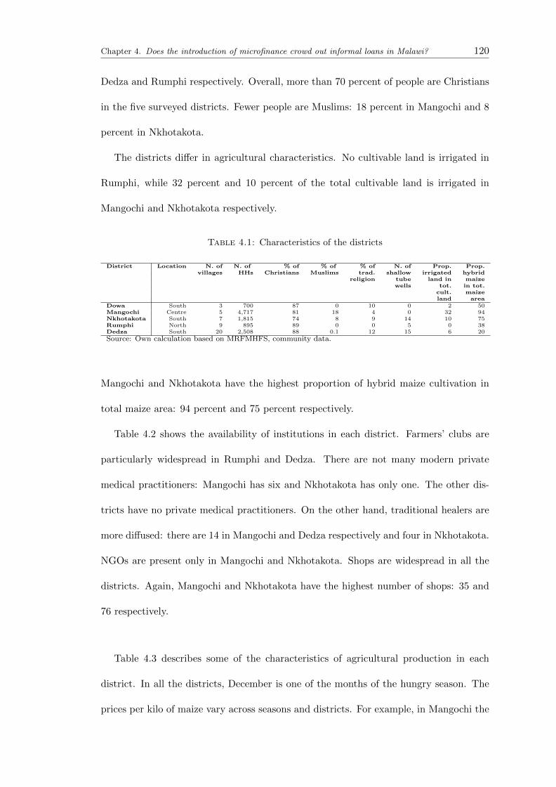
In spite of the diversities between these two countries, the widespread use of infor-
mal credit in Ethiopia and the government interventions in credit markets in Malawi
represent the ideal environment for answering the above mentioned research questions.
The two household surveys used in this thesis, the Ethiopian Rural Household Survey
and the Malawi Rural Financial Markets and Household Food Security, are very rich
data sets containing information about social and economic characteristics of the house-
holds as well as localities, and borrowing behaviour from formal and informal lenders.
As a consequence, they constitute an invaluable source of information to analyse the
characteristics and interaction of the formal and informal credit sectors.
Objectives
Chapter 1. Introduction 6
The specific objectives of each essay can be summarised as follows. The central idea
of the first essay is to develop an empirical model that can be of use in analysing the
determinants of participation in informal credit arrangements. We adopt an endogenous
switching regression model of access to informal credit where the availability of a partic-
ular type of informal arrangement varies across clusters in rural Ethiopia. This strategy
allows for taking into account substitutability between sources as well as household-
based and cluster-based socioeconomic characteristics.
The second essay exploits the idea that banks can acquire the local information they
lack (and that is readily available to informal lenders) in innovative ways. By creating
microfinance institutions, banks can crowd out informal borrowing. We adopt a policy
evaluation technique to test the effectiveness of this policy in Malawi.
Finally, the third essay uses information on the credit limit to explain the coexistence
of formal and informal credit sources in Malawi.
Although the essays are self-contained and focus on two different countries, a unified
story can be drawn from the thesis. If participation in informal arrangements depends
on the socioeconomic characteristics of households as well as clusters, one way for banks
to enter this market and exploit local information is to give borrowers incentives to use
their existing social linkages to the advantage of the banks. But information problems
are only part of the story, other market failures such as weak legal enforcement and the
low level of social capital may force the banks to ration credit and cause the persistence
of informal credit institutions. In addition, if the “social” motive1 for participation in
informal arrangements prevails over the “economic” motive, segmentation occurs despite
banks’ attempt to enter the market and complete crowding out will not be achieved.
The next section explains in detail the analysis and the contribution of each essay.
1See the next section for a summary of the sociological or cultural motive. A more detailed explanationof this approach is also contained in the second chapter.
Chapter 1. Introduction 7
1.3 Plan of the thesis
The three self-contained essays of this thesis focus on participation in informal credit
in rural Ethiopia, effect of microfinance institutions on informal borrowing and the
coexistence of formal and informal credit in Malawi. More specifically, the plan of the
thesis can be summarised as follows.
The second chapter reviews the theoretical and empirical literature on credit markets
comparing developed and developing countries. It provides a link between the three
essays of this thesis.
While credit markets in developed countries are dominated by the formal sector, in
developing economies - in particular sub-Saharan African countries - most of the loans
originate from informal sources. After highlighting risk and acquisition of durable goods
as motives for seeking credit (whether it be formal or informal), the literature review
focuses on two theories for the existence and diffusion of informal credit in developing
countries: the economic approach; and the cultural or sociological approach.
The economic approach maintains that informal finance arises as a response to credit
market failures. It is argued that market imperfections are more important in developing
economies at present for a variety of reasons. In developing economies such as in sub-
Saharan Africa informational sharing mechanisms tend to be small scale and localised,
markets are tightly interlinked, low levels of wealth limit the provision of collateral and
there are few scale economies [Bardhan and Udry, 1999; Besley, 1994; Gosh et al., 1999;
Ray, 1997]. In these circumstances, informal credit arrangements have an advantage as
they exploit low transaction costs [Kochar, 1997; Udry, 1990], screening is performed
through established relationships with borrowers [Aleem, 1990], and credit contracts are
flexible and customised with a chance to renegotiate repayments [Baydas et al., 1995].
Chapter 1. Introduction 8
The cultural or sociological approach, by contrast, sees informal institutions as far
less purposive than rational individuals engaged in maximising behaviour within some
constraints [Aryeetey and Udry, 1995; Azam et al., 2001; Fafchamps, 2002; Fafchamps
and Lund, 2003; Platteau, 2004; Udry, 1990]. According to this theory, norms of reci-
procity, intergenerational altruism and obligation involve households without having
been consciously devised [Granovetter, 1995].
Despite the numerous financial reforms aimed at facilitating the diffusion of formal
credit institutions in developing countires, we still observe the coexistence of formal and
informal credit arrangements. The literature typically focuses on two research areas, the
“spillover” or “residuality” theory and the markets segmentation theory.
This thesis specifically tests the “spillover” theory maintaining that the informal sec-
tor exists to satisfy the unmet demand for credit resulting from credit rationing in the
formal sector [for example, Banerjee and Duflo, 2001; Bell et al., 1997; Besley, 1994;
Bose and Cothrem, 1997; Eswaran and Kotwal, 1989].
On the other hand, according to the market segmentation theory the informal sector
may be the preferred source of credit for its unique characteristics, for the social prefer-
ences of the borrowers and for the specific purpose it is used [Barslund and Tarp, 2006;
Mohieldin and Wright, 2000].
The relative advantage of the informal sector over formal institutions may be an
object of concern as it can cause market inefficiency. This motivation together with dis-
tributional issues, vulnerability and poverty reduction call for government interventions
in credit markets. We look at two policies that could address these issues. The first
endeavours to create links between local moneylenders and banks. The second inter-
vention creates government-sponsored microfinance institutions. This thesis specifically
tests the effectiveness of the latter policy.
Chapter 1. Introduction 9
Chapter three is the first empirical essay and addresses the following research ques-
tion: “Why do households participate in informal credit institutions?” The chapter uses
as its primary source panel household data from the Ethiopian Rural Household Survey
(ERHS, 1994-1997). The contribution is to build a unified empirical model capable of
overcoming several limitations of the literature on this topic. We argue that the en-
dogenous switching regression model with principal components is able to identify the
following groups of factors that affect participation in informal credit.
The first group - household-based determinants such as wealth and demographic char-
acteristics - has been largely discussed in the literature [for example, Bose, 1998; Kochar,
1997; Pal, 2002; Ravi, 2003; Ray, 1997]. However, a limitation of these studies is that a
high degree of collinearity between household-specific variables limits the significance of
individual regressors. We overcome this problem by constructing principal components
of wealth variables.
The second group - idiosyncratic and aggregate shocks - has been analysed in the
literature as a motive for participation in credit markets [Bardhan and Udry, 1999;
Binswanger and Rosenzweig, 1993; Platteau and Abraham, 1987; Ruthenberg, 1971;
Townsend, 1994]. However, data availability limits the identification of different types
of shocks which may affect access to credit. The rich data in the ERHS allows for
the distinction between aggregate and idiosyncratic shocks, the former operating at the
cluster level and the latter at the household level.
The third group - cluster-based determinants such as demographic, infrastructural
and geographical characteristics - is often ignored in the literature due to limited data
and lack of appropriate models able to identify such characteristics. Knowledge of these
cluster-level determinants is as important as knowing why households utilise such insti-
tutions in clusters where they are available. With access to the village studies provided
Chapter 1. Introduction 10
by the ERHS, we have been able to identify dimensions of heterogeneity of access - most
notably social, geographic and economic characteristics - which may operate at a cluster
level, but are not identified at a household level [e.g. Fafchamps and Gubert, 2007].
The endogenous switching regression specification allows us to model the demand for a
particular type of informal credit as endogenously determined by household-based and
cluster-based determinants. Then, the access to informal credit is allowed to vary across
endogenously different clusters.
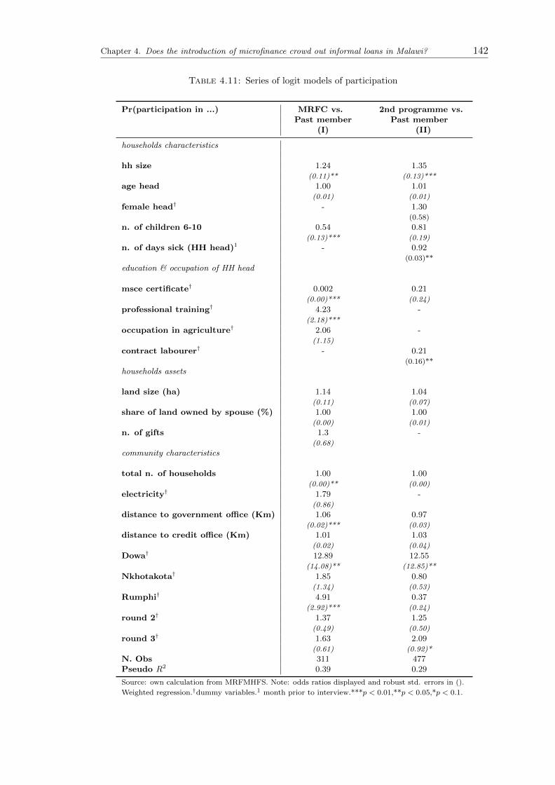
The fourth chapter is a policy-oriented empirical essay answering the following ques-
tion: “Do governments displace the informal loan market by introducing formal credit
institutions?” A policy that arises in response to market failures (one of the causes for
the diffusion of informal credit) aims at creating microfinance institutions that will ac-
quire information in innovative ways. By mimicking and exploting some of the features
of informal lending, banks can design credit contracts that harness local information and
give borrowers incentives to use their own information on their peers to the advantage
of the bank [Armendariz and Morduch, 2005; Ray, 1997].
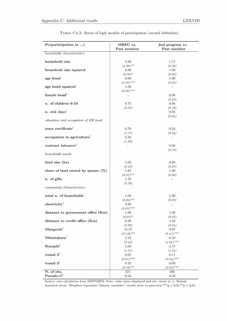
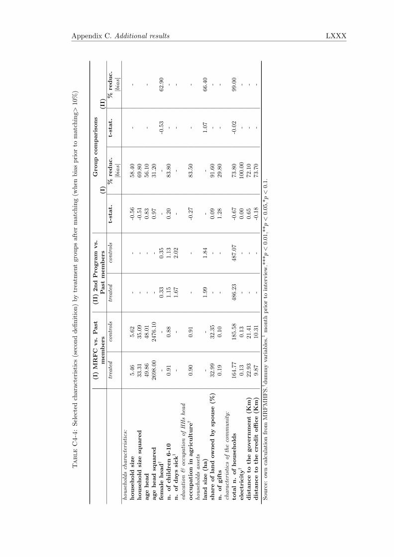
This essay evaluates the effectiveness of this policy by testing whether microfinance
institutions actually crowd out access to informal loans in Malawi. We adopt propen-
sity score matching to identify a causal relationship between access to formal credit
programmes and a reduction of informal borrowing. Propensity score matching is im-
plemented to match participants in microfinance programmes with households that have
similar observed characteristics (the so-called control group) and have been past partic-
ipants, but are not current members. We use the Malawi Rural Financial Markets and
Household Food Security (FMHFS, 1995), a rich survey containing information about
households’ borrowing behaviour.
The chapter introduces several innovations to the literature on crowding out. First,
Chapter 1. Introduction 11
few empirical studies have tested the crowding out hypothesis in the context of group-
lending institutions [for example, Mckernan et al., 2005].
Second, following the evaluation literature on training programmes [for example,
Brodaty et al., 2001; Frolich et al., 2004], we develop a model with multiple treatments
where households are classified as members of one, or more than one, group-lending pro-
gramme. This approach allows for a comparison between the effectiveness of different
credit programmes as well as between different groups of households. Does crowding out
differ with the economic status of the household? In particular, are relatively constrained
(unconstrained) households more (less) likely to reduce borrowing from informal lenders
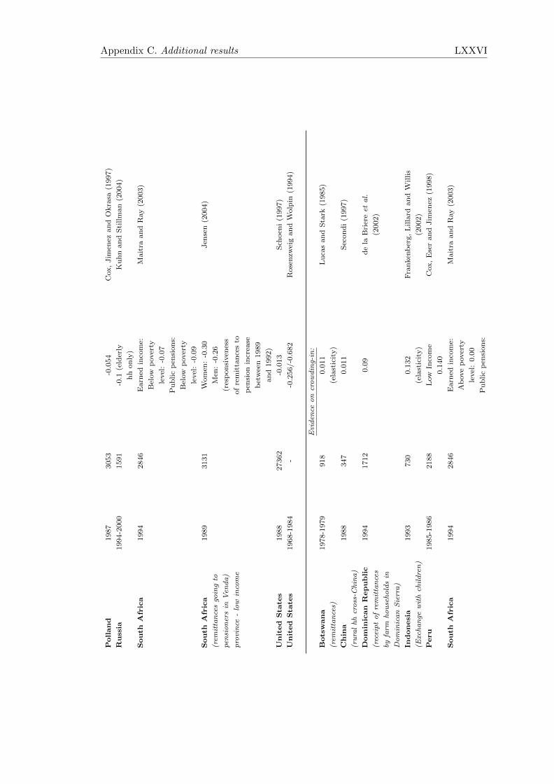
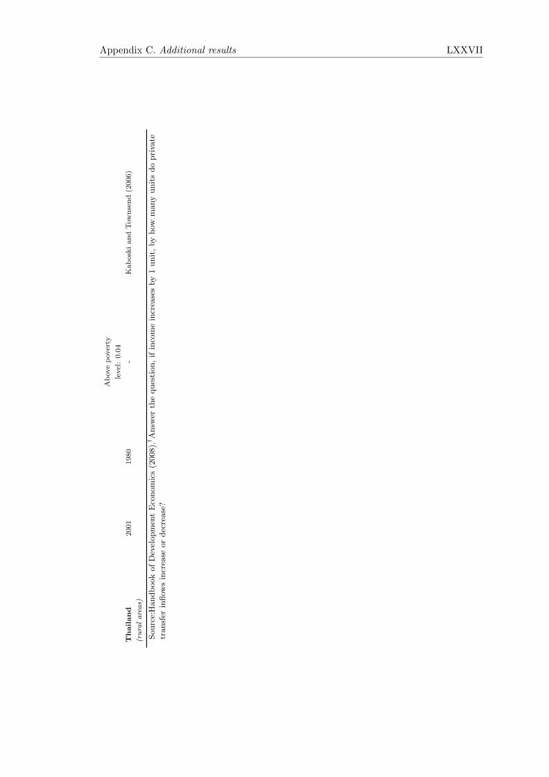
[Cox et al., 1998; Cox and Jimenez, 2005; Navajas et al. 2003]?
Third, nearly all the literature has focused on crowding out in the context of realised
transfers. Yet households’ demand for informal loans is also affected by the membership
in a microfinance programme not just by the actual borrowing [Cox and Fafchamps,
2008]. We evaluate the effects of both being a borrower and a member of microfinance
programmes.
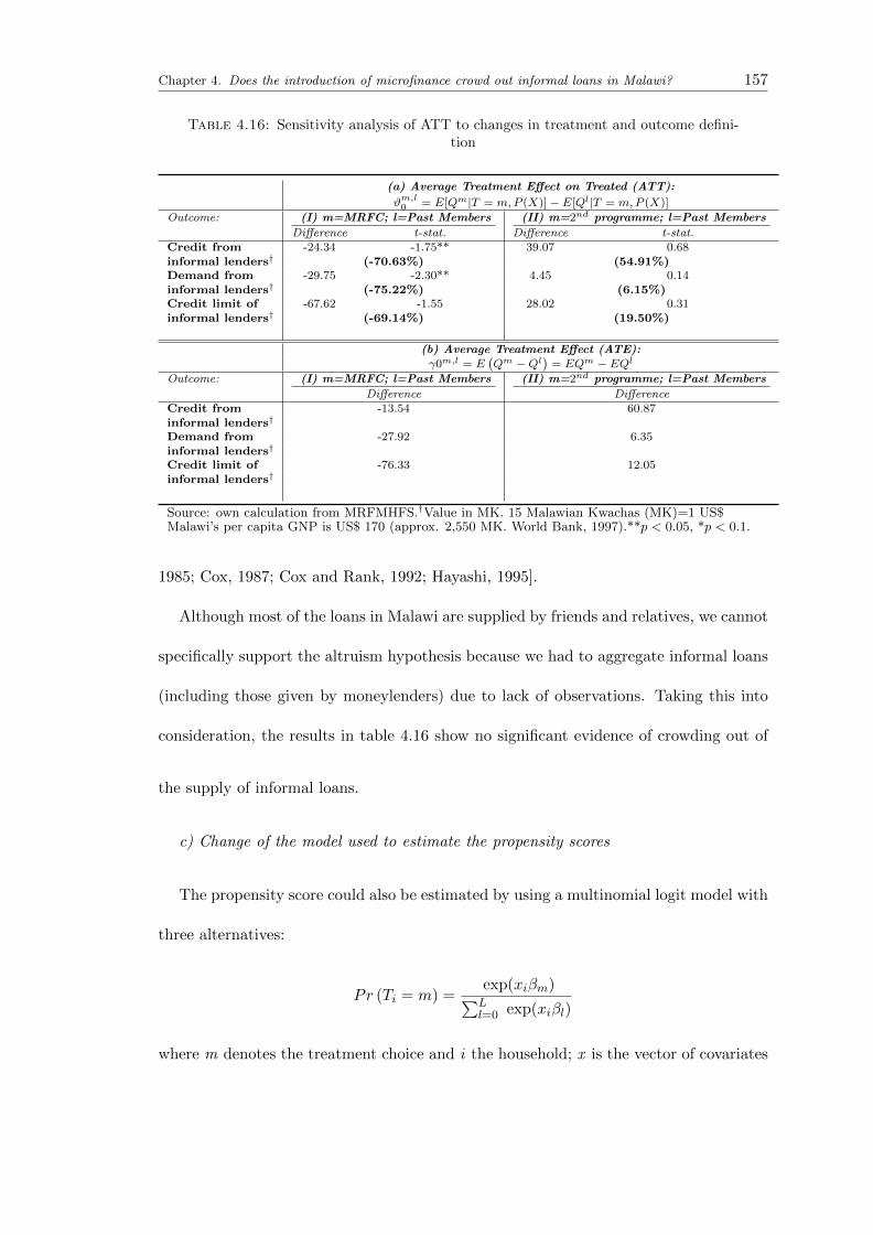
Fourth, most of the literature is only concerned with crowding out of the supply of
informal loans. This chapter disentangles demand and supply by employing outcome
variables such as demand and credit limit of informal loans2. Such detailed data is un-
common in many developed and developing countries.
Finally, we develop a rigorous sensitivity analysis by adopting a number of matching
algorithms and by testing for hidden biases arising from unobservable factors that affect
simultaneously the assignment into one of the programmes and the outcome variable.
Chapter five is the third empirical essay and addresses the question: “Why do formal
2The credit limit variable is extensively explained in chapter five. As it refers to the maximumamount the borrower thinks the lender is able to lend, it can be thought of as being the “supply” ofinformal loans.
Chapter 1. Introduction 12
and informal credit markets coexist?” In spite of recent financial liberalisation aimed
at broadening formal credit markets and in spite of interest rate differentials, in sub-
Saharan Africa formal and informal credit institutions persist in the same market. The
aim of this chapter is to motivate the partial crowding out effect found in the previous
essay. By using information on the credit limit provided in the Malawian survey we test
the spillover hypothesis, that is, the informal sector arises from a spillover demand from
the rationed formal sector.
This chapter also tests the liquidity constraints hypothesis, that is, an increase in the
credit limit should also affect the demand of liquidity constrained households. As the
spillover effect results from the existence of liquidity constraints, the spillover and the
liquidity constraints hypotheses are linked together.
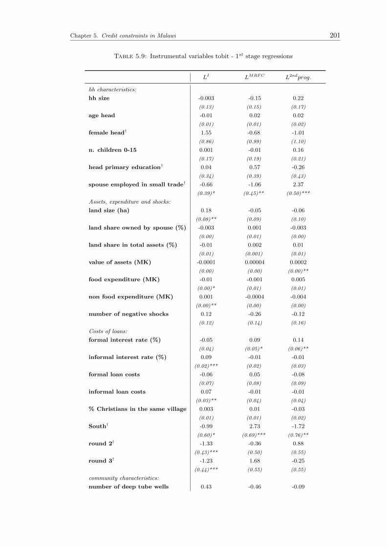
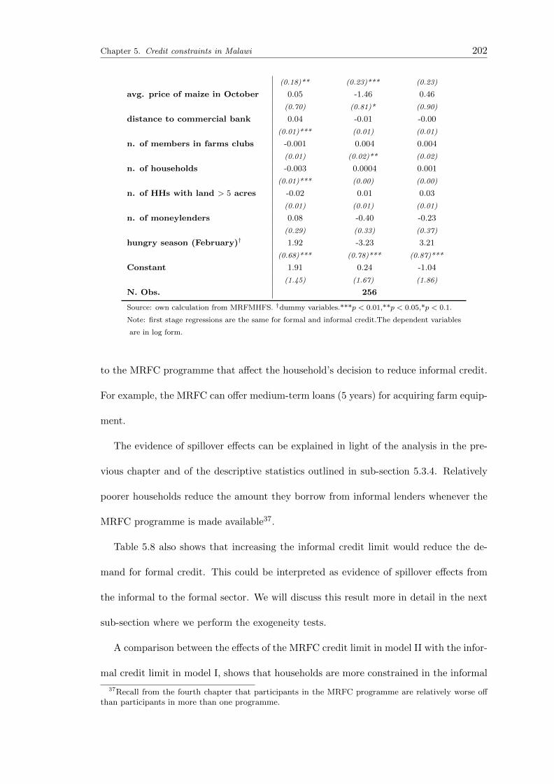
The chapter makes several contributions to the literature. First, it extends Diagne
(1999) and Diagne et al. (2000) approach by differentiating credit limits supplied by one
or more credit programmes.
Second, unlike previous studies that adopt a reduced form specification in which de-
mand and supply are collapsed into a single variable, we disentangle demand and supply
equations in two ways. The data set allows for the identification of the demand equa-
tion and the supply equation (which is the credit limit equation) for both applicants
and non-applicants to formal and informal lenders. In addition, following Diagne (1999)
and Grant (2007) we apply a number of exclusion restrictions to identify demand and
supply equations such as seasonal dummies and village characteristics.
Finally, we perform several robustness checks by addressing specification issues that
may seriously affect the results (for example, heteroskedasticity, non-normality and se-
lectivity).
Chapter six concludes the thesis with a brief summary of the findings. Limitations
Chapter 1. Introduction 13
of the approaches adopted in the thesis are also discussed. Finally, the chapter provides
some concluding remarks.
Chapter 2
Literature review
2.1 Introduction
In light of the research objectives outlined in the previous chapter, the literature
review is focused on the following issues. First, it gives an overview of credit market
institutions in Africa. Informal and formal credit arrangements are discussed in detail
with specific reference to Ethiopia and Malawi, the two countries on which this thesis is
focused.
Second, this chapter describes two motives for credit highlighted in the literature:
risk-coping and acquisition of durable goods.
Third, the literature review proceeds with an analysis of the motives for demanding
informal credit. It specifically focuses on the economic or market failure approach and
the sociological approach.
Finally, this chapter provides some motivations for government interventions in credit
markets arguing in favour of the creation of microfinance institutions.
14
Chapter 2. Literature review 15
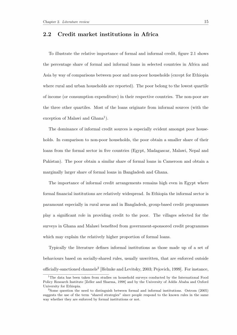
2.2 Credit market institutions in Africa
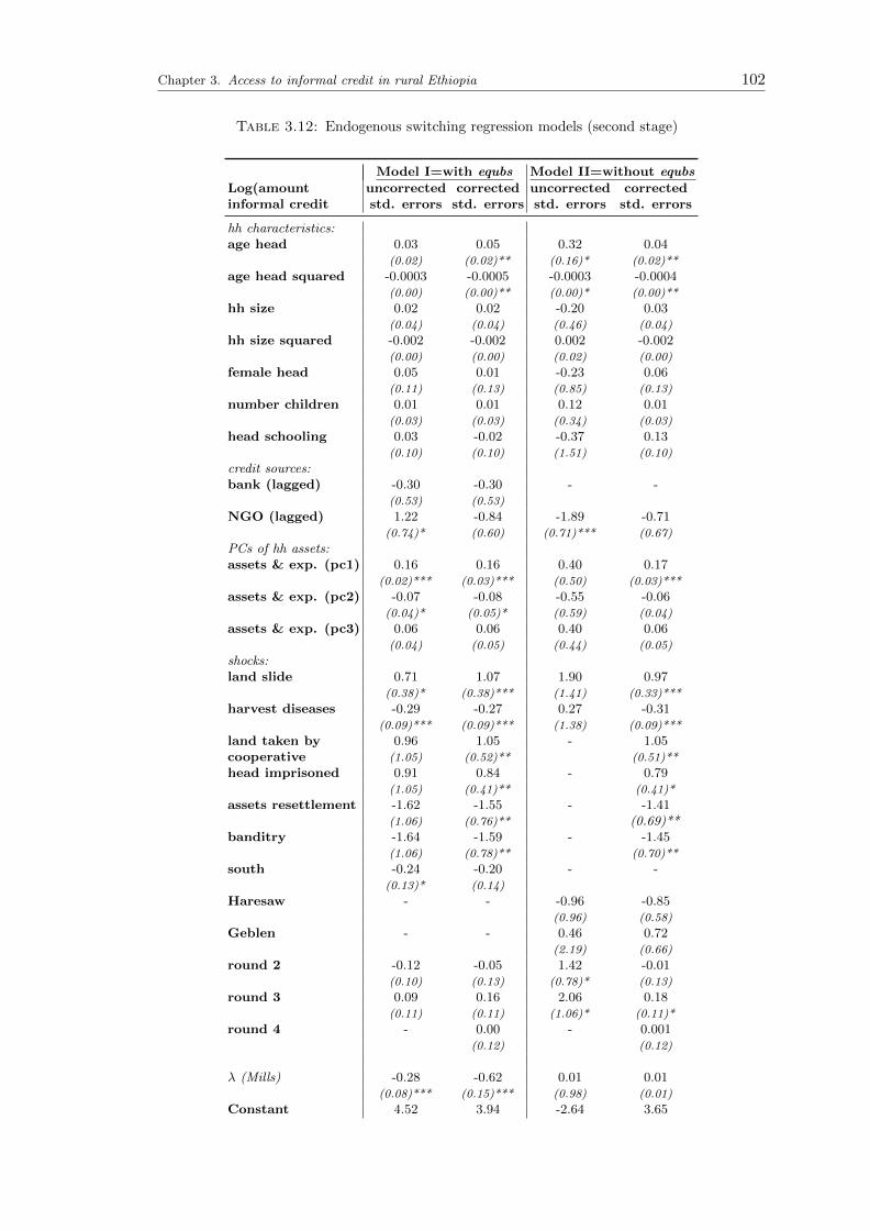
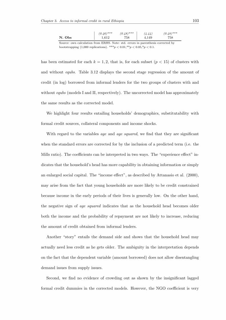
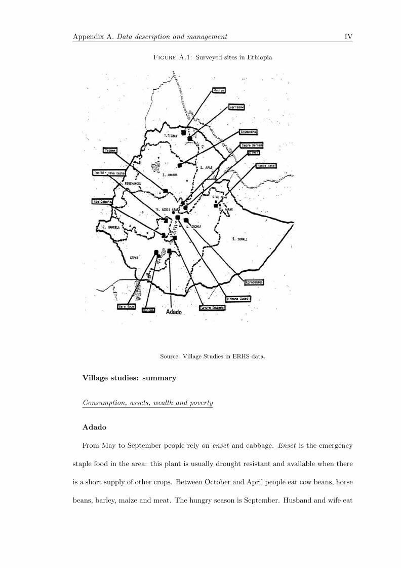
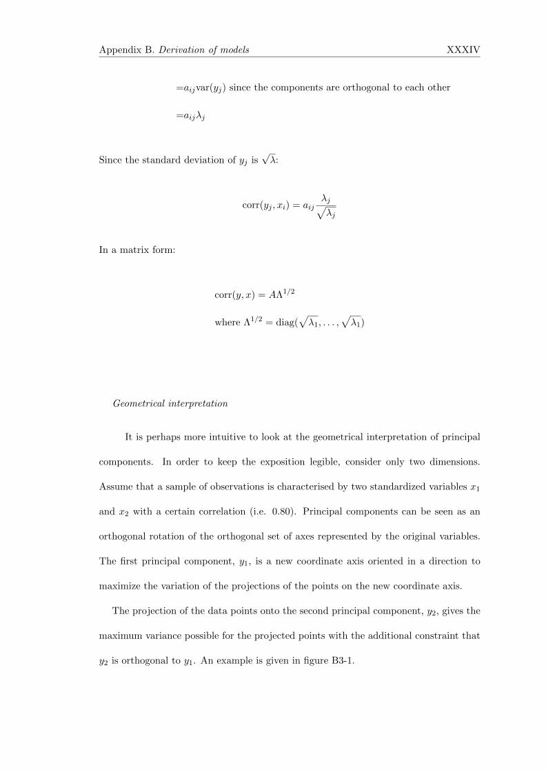
To illustrate the relative importance of formal and informal credit, figure 2.1 shows
the percentage share of formal and informal loans in selected countries in Africa and
Asia by way of comparisons between poor and non-poor households (except for Ethiopia
where rural and urban households are reported). The poor belong to the lowest quartile
of income (or consumption expenditure) in their respective countries. The non-poor are
the three other quartiles. Most of the loans originate from informal sources (with the
exception of Malawi and Ghana1).
The dominance of informal credit sources is especially evident amongst poor house-
holds. In comparison to non-poor households, the poor obtain a smaller share of their
loans from the formal sector in five countries (Egypt, Madagascar, Malawi, Nepal and
Pakistan). The poor obtain a similar share of formal loans in Cameroon and obtain a
marginally larger share of formal loans in Bangladesh and Ghana.
The importance of informal credit arrangements remains high even in Egypt where
formal financial institutions are relatively widespread. In Ethiopia the informal sector is
paramount especially in rural areas and in Bangladesh, group-based credit programmes
play a significant role in providing credit to the poor. The villages selected for the
surveys in Ghana and Malawi benefited from government-sponsored credit programmes
which may explain the relatively higher proportion of formal loans.
Typically the literature defines informal institutions as those made up of a set of
behaviours based on socially-shared rules, usually unwritten, that are enforced outside
officially-sanctioned channels2 [Helmke and Levitsky, 2003; Pejovich, 1999]. For instance,
1The data has been taken from studies on household surveys conducted by the International FoodPolicy Research Institute [Zeller and Sharma, 1998] and by the University of Addis Ababa and OxfordUniversity for Ethiopia.
2Some question the need to distinguish between formal and informal institutions. Ostrom (2005)suggests the use of the term “shared strategies” since people respond to the known rules in the sameway whether they are enforced by formal institutions or not.
Chapter 2. Literature review 16
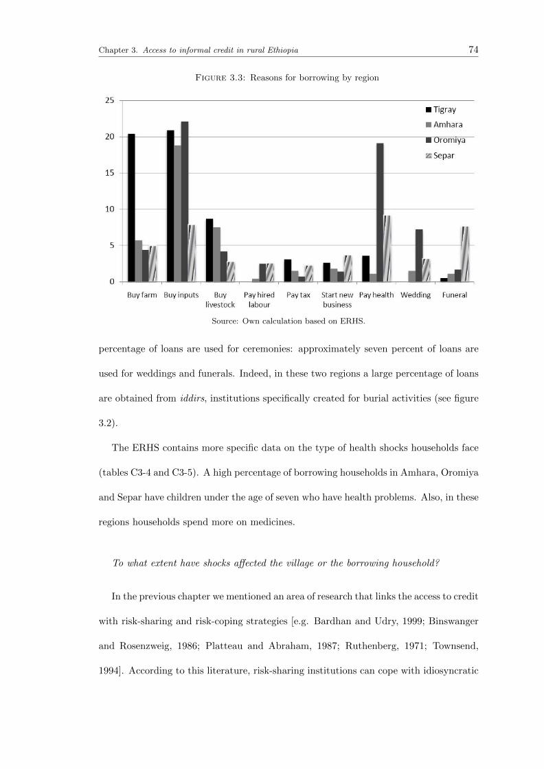
Figure 2.1: Share of formal and informal loans in selected countries in Africa andAsia
Note: ”P” and ”NP” refer to poor and non-poor households respectively. Source: Zeller and
Sharma (1998), Ibrahim, Kedir and Torres (2007) and our own calculations from the ERHS.
informal finance consists of often unrecorded lending activities that take place outside
formal financial institutions.
Informal financial institutions vary in their operational features: some are community
or group-based whilst others are individual. They vary in their scope - some are involved
in either savings or lending, whilst others are involved in both. They can involve cash,
payment in-kind transactions or both. Moneylenders, friends and relatives, rotating
savings and credit associations (RoSCAs) and self-help groups are examples of informal
credit institutions.
Numerous studies have shown that informal financial arrangements across Africa
exhibit diversity [Aryeetey and Hyuha, 1991; Chipeta and Mkandawire, 1991; Soyibo,
1996]. Each informal arrangement typically covers a limited geographical area and of-
ten takes place among people linked by contracts (i.e. landlord-tenant), among kins-
Chapter 2. Literature review 17
men or people in the same locality. On the other hand, formal finance comprises of
institutions regulated by the government and the Central Bank operating within the
regulatory framework of the financial system and generally provides services on a more
geographically dispersed basis. Examples include commercial banks, agricultural banks
and government-sponsored microfinance institutions.
The large spectrum of credit institutions can be stratified according to two criteria.
The first stratifies according to an increasing level of formality as referred to above. The
second criterion refers to the degree of social cohesion, ordered in a roughly decreasing
level of lender-borrower closeness and exogeneity of the lending methodology [Robinson
and Schmid, 1988; van Bastelaer, 2000; Woolcock and Narayan, 2000].
Figure 2.2: Segments of financial systems
Source: Own classification.
Figure 2.2 illustrates informal and formal credit institutions ordered in an increasing
degree of formality and decreasing level of social cohesion. In this context, informal
institutions appear at the top of the scale due to their low level of formality and high
degree of social cohesion. As formal institutions have a high level of formality and low
degree of social cohesion, they appear at the lower end of the scale of credit institutions.
Chapter 2. Literature review 18
2.3 Informal credit institutions
2.3.1 Friends and relatives
Friends and relatives provide sources of financial (and other) help through the high-
est degree of social cohesion. The fact that both lender and borrower know each other
dispenses with the key features of formal credit transactions such as ensuring credit
worthiness or demanding collateral and guarantees. Usually loans are supplied with-
out interest repayments or regular repayment schedules and transaction records are not
made. Such lenders provide loans on a need-based manner [Fafchamps, 2008]. Sanctions
often include denial of future loans or other social costs (such as “bad” reputation within
the community) in case of default.
A disadvantage of this source of lending is the limited and often irregular supply of
loans. That is, only when the individual has surplus funds is the loan made.
Credit given by friends and relatives often implies an obligation for future recipro-
cation. Thomas and Worrall (2000) note that if the costs of giving are covered by the
perceived benefits of future reciprocity, then often these forms of informal credit are
likely to be more effective than other informal or formal institutions.
The importance of these types of informal networks is now recognised especially in
small communities. For example, Sahlins (1972) reported a mechanism of “generalised
reciprocity” in which those with high income help those with low income. Similar mutual
help contracts have been described by Platteau and Abraham (1987) who found evidence
of reciprocal credit among a community of fishermen in an Indian village. Udry (1990)
found evidence of credit with repayments contingent on the realization of production in
Northern Nigeria. Reciprocity may be stronger among ethnically homogenous groups,
family, clan or religious affiliations because these groups can threaten to impose larger
Chapter 2. Literature review 19
punishments on individuals breaking the mutual insurance arrangements.
Gachter and Herrmann (2009) demonstrate with laboratory experiments in Russia
and Switzerland that many people are “strong reciprocators” who cooperate and punish
others even if there are no gains from future reciprocity or other reputational gains.
They show that patterns of strong reciprocity can be explained by cultural differences
across the two countries.
2.3.2 Mutual help associations
Further down the scale of credit institutions, there are a series of mutual, often local,
helping associations. For example, in Ethiopia there are a number of mutual assistance
associations called iddir and the RoSCA-type called equb [Aredo, 1993; Mauri, 1987].
i) RoSCAs
The nature of RoSCAs was originally analysed within the anthropological literature.
Geertz (1962) described RoSCAs as a “middle-rung” institution. He defined it as “a shift
from a traditionalistic agrarian society to an increasingly fluid commercial one”, and as
an “educational mechanism in terms of which peasants learn to be traders, not merely
in the narrow occupational sense, but in the broad cultural sense”. Regarding their
functionality, Geertz (1962) pointed out that RoSCAs are “... a lump sum fund composed
of fixed contributions from each member of the association which is distributed, at
fixed intervals and as a whole, to each member of the association in turn”. Ardener
(1964), however, argued that this definition is too restrictive and defined RoSCAs as “an
association formed upon a core of participants who agree to make regular contributions
to a fund which is given, in whole or in part, to each contributor in rotation”. The fund
or “pot” is allocated to one member by drawing or bidding. At the end of each round
Chapter 2. Literature review 20
past winners are excluded from receiving the pot.
Although little is known about their origin, RoSCAs are not restricted to any country.
Ardener (1964) had already reported a well-developed RoSCA in Asia at the end of the
nineteenth century. In Ghana, RoSCAs are found in larger towns but not in rural areas.
In Egypt, RoSCAs are known as gameya and have existed for more than fifty years.
Rural areas see membership confined to women, but in urban areas men, women and
children belong to them [Ardener, 1964].
The principal function of RoSCAs is to assist capital-formation, or more simply to
create savings. As some individuals feel that they would struggle to save if they were
not committed to such a group, contributions can be seen as a form of forced saving. In
addition, women may see it as a way to prevent their husbands using family savings for
personal consumption (for instance on alcohol or cigarettes).
In relatively recent years, RoSCAs have been subject to a more formal economic
analysis. For example, Besley et al. (1993) analyse the economic rationale of RoSCAs.
This paper compares the random and bidding RoSCAs. In the former “people commit
to putting fixed sum of money into a “pot” for each period of life of the RoSCA. The pot
is randomly allocated to one of the members. In the next period, the process repeats
itself, except that the previous winner is excluded from the draw of the pot. The process
continues until each member of the RoSCA has received the pot once”.
The bidding RoSCA is similar to the random RoSCA, except that the pot may be
obtained earlier if one member bids more than the others. “The bidding process merely
establishes the priority”.
Besley et al. (1993) show that both random and bidding RoSCAs improve members
welfare compared to the autarky level. However, in the bidding RoSCA each member has
a different rate of nondurable consumption during the accumulation period (i.e. those
Chapter 2. Literature review 21
who get the pot earlier, make higher contributions and consume less of the nondurable;
the last member getting the pot makes no contribution and must have greater nondurable
consumption during accumulation than under autarky). Moreover, Besley et al. (1993)
demonstrate that random RoSCAs are better than bidding RoSCAs because the random
allocation dominates ex ante the bidding one (ex post this may not be true for the last
“bidder”).
Besley et al. (1996) show that RoSCAs in Taiwan allow members to reduce the time
to acquire a durable good. This thesis pins down the factors affecting the formation of
RoSCAs in rural Ethiopia.
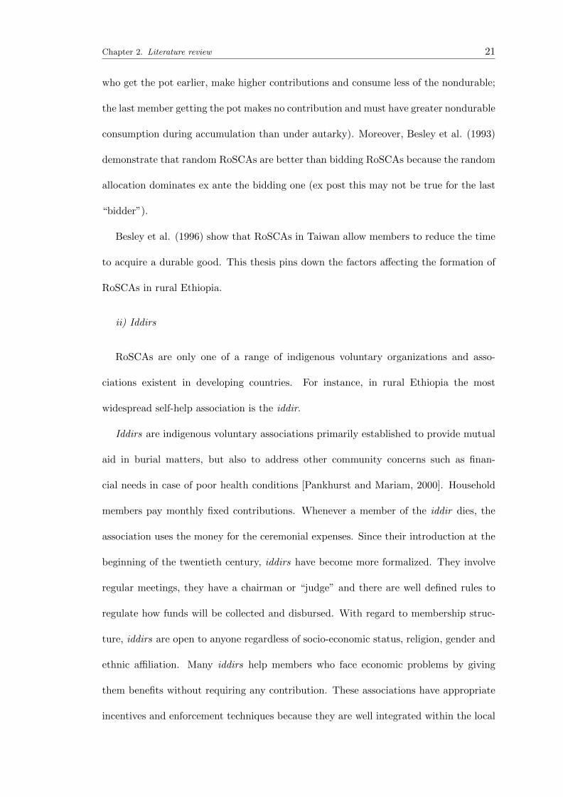
ii) Iddirs
RoSCAs are only one of a range of indigenous voluntary organizations and asso-
ciations existent in developing countries. For instance, in rural Ethiopia the most
widespread self-help association is the iddir.
Iddirs are indigenous voluntary associations primarily established to provide mutual
aid in burial matters, but also to address other community concerns such as finan-
cial needs in case of poor health conditions [Pankhurst and Mariam, 2000]. Household
members pay monthly fixed contributions. Whenever a member of the iddir dies, the
association uses the money for the ceremonial expenses. Since their introduction at the
beginning of the twentieth century, iddirs have become more formalized. They involve
regular meetings, they have a chairman or “judge” and there are well defined rules to
regulate how funds will be collected and disbursed. With regard to membership struc-
ture, iddirs are open to anyone regardless of socio-economic status, religion, gender and
ethnic affiliation. Many iddirs help members who face economic problems by giving
them benefits without requiring any contribution. These associations have appropriate
incentives and enforcement techniques because they are well integrated within the local
Chapter 2. Literature review 22
communities. For example, a person who does not belong to an iddir is considered a
disgrace to his or her family. In comparison to some formal sources, RoSCAs and iddirs
are less impersonal.
2.3.3 Moneylenders
Moneylending is characterised by a more exogenous lending methodology and often
by a lower level of social cohesion. Stiglitz (1990) noted that “the local moneylenders
have one important advantage over the formal [lending] institutions: they have more
detailed knowledge of the borrowers. They therefore can separate out high-risk and
low-risk borrowers and charge them appropriate interest rates”. Moneylenders provide
flexible contract terms and dispense with the need for collateral due to the information
they possess on borrowers. They usually charge high rates of interest in comparison to
formal lending institutions.
Moneylenders may borrow from banks during high demand for credit by using their
own funds as security, thus creating a channel where formal funds are injected into the
informal sector.
Mansuri (2007) reported that often moneylenders’ primary activity is not lending:
loans are means of obtaining a return on other transactions in which both lender and
borrower are involved. The interweaving of activities between borrowers and lenders
allows the lender to gather information about the borrowers’ ability to repay. The re-
lationship between moneylender and borrower is reminiscent of a patron-client vertical
interaction. It is intrinsically unequal as the moneylender has access to several methods
(such as lowering the wage if the moneylender is also the employer) to ensure repayment
[van Bastelaer, 2000]. Badhuri (1973) observed that perpetual indebtedness of the bor-
rower as a consequence of high interest rates is characteristic of a semi-feudal environ-
Chapter 2. Literature review 23
ment. The loan is used as a way to secure asset transfers or long-term relationships with
the borrowers.
2.4 Formal credit institutions
As stated above, formal or institutional lenders can be placed further down in the
scale of credit institutions when classified in this way due to their low degree of social
cohesion.
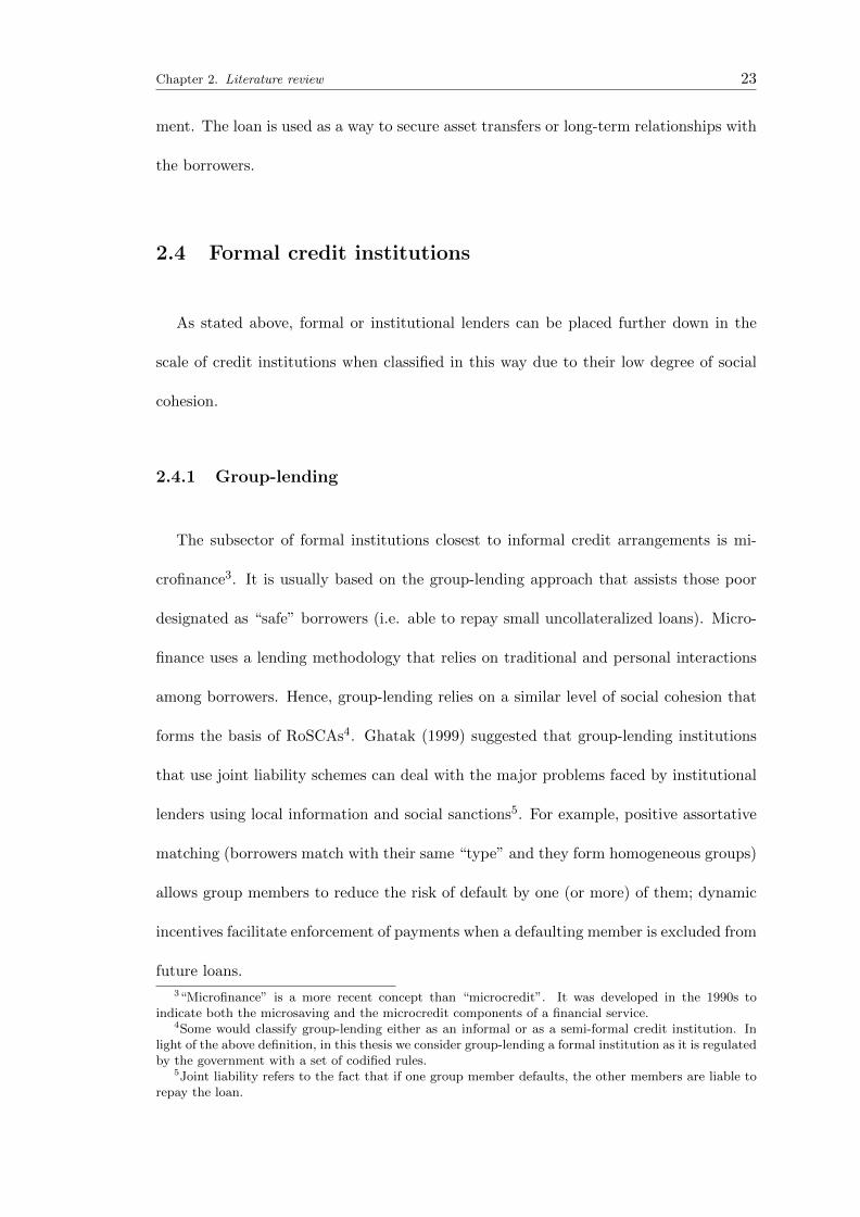
2.4.1 Group-lending
The subsector of formal institutions closest to informal credit arrangements is mi-
crofinance3. It is usually based on the group-lending approach that assists those poor
designated as “safe” borrowers (i.e. able to repay small uncollateralized loans). Micro-
finance uses a lending methodology that relies on traditional and personal interactions
among borrowers. Hence, group-lending relies on a similar level of social cohesion that
forms the basis of RoSCAs4. Ghatak (1999) suggested that group-lending institutions
that use joint liability schemes can deal with the major problems faced by institutional
lenders using local information and social sanctions5. For example, positive assortative
matching (borrowers match with their same “type” and they form homogeneous groups)
allows group members to reduce the risk of default by one (or more) of them; dynamic
incentives facilitate enforcement of payments when a defaulting member is excluded from
future loans.
3“Microfinance” is a more recent concept than “microcredit”. It was developed in the 1990s toindicate both the microsaving and the microcredit components of a financial service.
4Some would classify group-lending either as an informal or as a semi-formal credit institution. Inlight of the above definition, in this thesis we consider group-lending a formal institution as it is regulatedby the government with a set of codified rules.
5Joint liability refers to the fact that if one group member defaults, the other members are liable torepay the loan.
Chapter 2. Literature review 24
However, there are also some disadvantages to group-lending, for example group size
decreases once social sanctions are applied [Impavido, 1998]. Second, the degree to
which group members know each other and interact on a regular basis also affects the
performance of the group. Third, group repayments are negatively affected by aggregate
shocks (i.e. shocks that affect all members of a community).
Although the group-based approach has developed in the 1970s, the concept is a cen-
tury old. Ghatak and Guinnane (1998) and Woolcock and Narayan (2000) pointed out
the existence of a German credit cooperative in the mid-nineteenth century. Today the
most studied example of group-based lending is the Grameen Bank in Bangladesh. The
Grameen Bank was founded in 1976 by Mohammad Yunus, a professor at the University
of Chittagong, as a research project. By 1994, the Grameen Bank had served half of
all villages in Bangladesh, with a total membership of more than two million, of which
94 percent were women. It uses group-lending and joint liability schemes where small
uncollateralized loans are repaid in weekly instalments. If any member of the group
defaults, the whole group is denied future credit. Using this approach, the Grameen
Bank has consistently reported repayment rates in excess of 95 percent.
Since its foundation, the Grameen Bank model has been exported to many countries
throughout Africa, Latin America and Asia. It was replicated in Malawi (one of the
countries on which this thesis is focused) in 1987 when the World Bank and the Inter-
national Fund for Agricultural Development (IFAD) funded the Mudzi Fund. Another
replication of the model was founded in 1986 when Bolivian business leaders established
a non-profit microlending entity called PRODEM. In 1992, PRODEM became Bancosol
after a privatisation process. By 1997 Bancosol was the first microfinance institution to
issue dividends to shareholders.
Chapter 2. Literature review 25
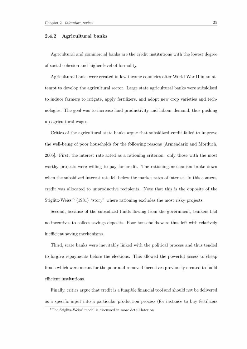
2.4.2 Agricultural banks
Agricultural and commercial banks are the credit institutions with the lowest degree
of social cohesion and higher level of formality.
Agricultural banks were created in low-income countries after World War II in an at-
tempt to develop the agricultural sector. Large state agricultural banks were subsidised
to induce farmers to irrigate, apply fertilizers, and adopt new crop varieties and tech-
nologies. The goal was to increase land productivity and labour demand, thus pushing
up agricultural wages.
Critics of the agricultural state banks argue that subsidized credit failed to improve
the well-being of poor households for the following reasons [Armendariz and Morduch,
2005]. First, the interest rate acted as a rationing criterion: only those with the most
worthy projects were willing to pay for credit. The rationing mechanism broke down
when the subsidized interest rate fell below the market rates of interest. In this context,
credit was allocated to unproductive recipients. Note that this is the opposite of the
Stiglitz-Weiss’6 (1981) “story” where rationing excludes the most risky projects.
Second, because of the subsidized funds flowing from the government, bankers had
no incentives to collect savings deposits. Poor households were thus left with relatively
inefficient saving mechanisms.
Third, state banks were inevitably linked with the political process and thus tended
to forgive repayments before the elections. This allowed the powerful access to cheap
funds which were meant for the poor and removed incentives previously created to build
efficient institutions.
Finally, critics argue that credit is a fungible financial tool and should not be delivered
as a specific input into a particular production process (for instance to buy fertilizers
6The Stiglitz-Weiss’ model is discussed in more detail later on.
Chapter 2. Literature review 26
for farm production).
On the other hand, recent empirical work by Burgess and Pande (2005) showed net
positive average impacts of India’s Integrated Rural Development Programme (IRDP)
on the poor. According to Burgess and Pande (2005), the expansion of access to informal
finance enabled people to increase non-agricultural production activities. As the eco-
nomic returns from these activities were higher than those from agricultural activities,
the IRDP was able to reduce rural poverty. Nevertheless, the programme was ended
in 1990 because the expansion of rural bank branches was too expensive. High default
rates and subsidised interest rates are testimony of the fact that rural branches were a
policy vehicle for costly redistribution of resources to rural areas.
Binswanger and Khandker (1995) found that between 1972-1973 and 1980-1981 state
agricultural banks in India had increased rural wages and employment. However, as
they found only modest impacts on agricultural output, they concluded that the costs
of such government programmes were much higher than the economic benefits.
In 1970 the Agricultural and Development Bank was established in Ethiopia. It is
government-owned and provides short term loans to the agricultural sector, medium and
long-term loans to individuals, cooperatives and agricultural projects as well as special
credit lines for microenterprises. Additionally, the Agricultural and Development Bank
offers banking services like current and saving accounts.
2.4.3 Commercial banks
Private, domestic commercial banks are a relatively recent phenomenon in many
developing countries, especially in Africa. From the 1950s to the 1970s, banks were
predominantly owned by the government or by other foreign commercial banks. The
Chapter 2. Literature review 27
existing local banks were typically relatively small and often served a closed set of busi-
ness groups.
In most developing countries, up to the 1980s, it was the highly regulated formal
financial markets that were responsible for the inadequate development of privately-
owned commercial banks due to their interest rate ceilings, high reserve requirements
and directed credit lines. Banks could not charge sufficiently high interest rates to cover
the costs and risks of lending to a large clientele.
In the 1980s the financial liberalization process allowed private domestic commercial
banking to expand rapidly. New private banks were used to obtain funds for businesses
and corporations.
At that time the government of Malawi, for example, implemented measures to lib-
eralize its financial sector. Reforms included the elimination of agricultural subsidies
and interest rate controls along with the removal of exchange control regulations and
restrictions on capital movements. This liberalization process has increased the number
of players in Malawi’s financial markets. It has eight commercial banks providing sav-
ings, lending and other investment products. Two major banks, the National Bank of
Malawi and Stanbic Bank, dominate the financial sector with 58 percent of the sector’s
assets and 59 percent of its deposits7. The National Bank of Malawi is predominantly
owned by companies with significant government shareholdings. The Standard Bank of
South Africa now holds a 60 percent shareholding in Stanbic Bank (formerly known as
the Commercial Bank of Malawi when it was controlled by the government).
In Ethiopia, the financial liberalization process initiated in 1992 was much less rad-
ical than elsewhere in Africa. The commitment to continued government ownership of
existing financial institutions was still strong and the government was reluctant to allow
foreign banks in Ethiopia.
7This data has been reported by the United Nations Capital Development Fund, 2006.
Chapter 2. Literature review 28
Since the financial reforms began, new financial institutions have been allowed to
operate in Ethiopia. Six private banks and eight insurance companies now operate
alongside public ones. Although the government-owned Commercial Bank of Ethiopia
(CBE) remains the country’s largest commercial bank, its dominance is declining as
private banks and competition from international banks grow.
From 1994 the CBE obtained greater autonomy in its lending decisions and acquired
its own Board of Directors. A few years ago, the government restructured the CBE and
signed a contract with the Royal Bank of Scotland for management consultancy services.
In January 2009, the Commercial Bank of Ethiopia received regulatory approval to open
a branch in Southern Sudan.
2.5 Why do households demand credit?
There are two primary motives for households seeking credit. First, households use
credit to cope with shocks that may appear in their lifetime (“the risk motive”). Sec-
ondly, credit may be required to purchase “lumpy” assets - typically, durable goods.
Whilst the empirical analysis carried out in this thesis explicitly focuses on the risk
motive for credit, the following sub-sections will analyse each of these motives in turn.
2.5.1 Risk
Risk pervades all of life’s activities. It causes fluctuations in income and health.
These fluctuations can be predictable or unpredictable. Risk can affect us individually
(so-called idiosyncratic shocks such as illness) or can affect the entire community (so-
called aggregate shocks such as natural disasters or fluctuations in prices that affect the
entire economy).
Chapter 2. Literature review 29
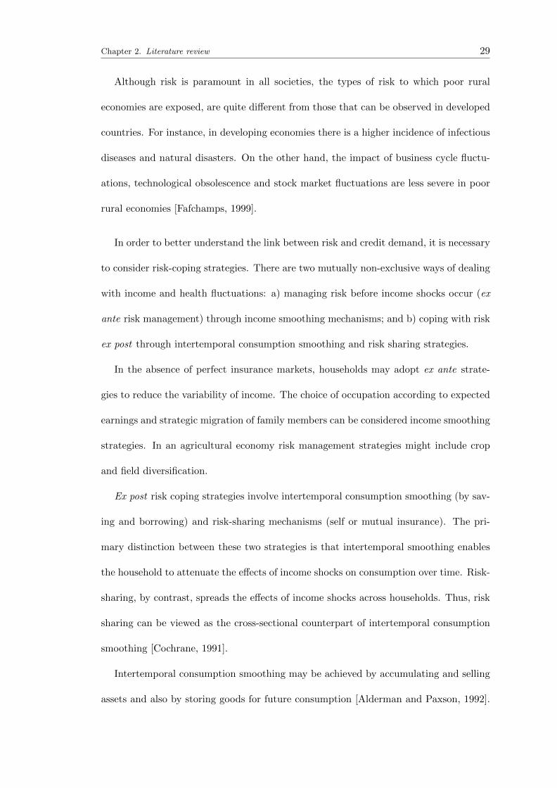
Although risk is paramount in all societies, the types of risk to which poor rural
economies are exposed, are quite different from those that can be observed in developed
countries. For instance, in developing economies there is a higher incidence of infectious
diseases and natural disasters. On the other hand, the impact of business cycle fluctu-
ations, technological obsolescence and stock market fluctuations are less severe in poor
rural economies [Fafchamps, 1999].
In order to better understand the link between risk and credit demand, it is necessary
to consider risk-coping strategies. There are two mutually non-exclusive ways of dealing
with income and health fluctuations: a) managing risk before income shocks occur (ex
ante risk management) through income smoothing mechanisms; and b) coping with risk
ex post through intertemporal consumption smoothing and risk sharing strategies.
In the absence of perfect insurance markets, households may adopt ex ante strate-
gies to reduce the variability of income. The choice of occupation according to expected
earnings and strategic migration of family members can be considered income smoothing
strategies. In an agricultural economy risk management strategies might include crop
and field diversification.
Ex post risk coping strategies involve intertemporal consumption smoothing (by sav-
ing and borrowing) and risk-sharing mechanisms (self or mutual insurance). The pri-
mary distinction between these two strategies is that intertemporal smoothing enables
the household to attenuate the effects of income shocks on consumption over time. Risk-
sharing, by contrast, spreads the effects of income shocks across households. Thus, risk
sharing can be viewed as the cross-sectional counterpart of intertemporal consumption
smoothing [Cochrane, 1991].
Intertemporal consumption smoothing may be achieved by accumulating and selling
assets and also by storing goods for future consumption [Alderman and Paxson, 1992].
Chapter 2. Literature review 30
Risk-sharing may be accomplished through formal institutions and informal arrange-
ments. Examples of the former include insurance and futures markets whilst examples
of the latter include state-contingent transfers and remittances between friends and rel-
atives.
2.5.1.1 Intertemporal consumption smoothing
Intertemporal smoothing allows consumption to be insulated from the effects of in-
come fluctuations by using saving and credit transactions. In Friedman’s permanent
income hypothesis (PIH) model, consumers try to smooth out spending based on their
estimates of permanent income [Friedman, 1957]. Only if there has been a change in
permanent income will there be a change in consumption. Indeed, the PIH states that
transitory changes in income do not affect consumer spending behaviour in the long run.
The permanent income hypothesis (PIH) is derived from a partial equilibrium model
which involves a representative household, taking prices as given. A representative
household maximises expected utility subject to a constraint where the household re-
ceives a random income y and decides how to allocate its resources between consumption
and net saving for the next period. The solution to the problem is given by the following
equation:
E
u′(ct+1)
u′(ct)
=
1
β(1 + rt)(2.1)
where r is the interest rate and β is the discount factor (bounded between zero and one).
Equation 2.1 shows that the intertemporal ratio of marginal utilities depends on the
discount factor and the interest rate. Whenever β(1 + r) = 1, the marginal utility of
consumption is a martingale process. Households save over time in order to create a
buffer stock for precautionary reasons. In addition or alternatively households borrow
Chapter 2. Literature review 31
from credit markets.
If households experienced an adverse shock, the average propensity to consume would
increase. In the light of the uncertainty surrounding the adverse shock, households would
be prepared to take loans, even with high interest rates, to get through the bad period.
As referred to above, households could also cope with risk by creating buffer stock
savings. Following Deaton (1992), suppose that the marginal utility of consumption is
convex. Note that the convexity of the marginal utility (third derivative of the utility)
tells us how prudent households are. This concept is different from the degree of risk
aversion (second derivative of the utility). Only in the special case of iso-elastic utility
are the two concepts equivalents. In addition, assume that the variability of consumption
increases, thus creating more uncertainty. The increase in (mean-preserving) spread will
increase the expected value and the marginal utility of consumption. As a consequence,
consumption decreases and savings increase. When households are more prudent, an
increase in uncertainty enhances precautionary savings [Banks et al., 2001].
The PIH has been criticised for the assumption of perfect capital markets [Maki,
1993]. When capital markets are imperfect, the optimal consumption path is different to
the one specified in the PIH because households cannot create a “cushion” of marketable
assets and do not have the capacity to borrow up to the value of prospective lifetime
wealth against future earnings [Ishikawa, 1974; Pissarides, 1978].
The deviation from the life cycle (LC) and permanent income hypothesis (PIH) has
been used to indirectly infer the presence of credit constraints. One of the testable
implications of the LC/PIH is that in the absence of liquidity and borrowing constraints,
transitory income shocks do not affect consumption [Deaton, 1992; Hall, 1978].
Empirical tests for the presence of credit constraints based on the LC/PIH use house-
hold consumption and income data to look for a significant dependence (or “excess
Chapter 2. Literature review 32
sensitivity”) of consumption on transitory income. Evidences of liquidity constraints
as a result of imperfect capital markets have been provided in both developed and
developing countries as shown below.
However, the LC/PIH approach to detect credit constraints may be inconclusive.
First, deviations from the LC/PIH can result from prudent or cautionary behaviour even
if the borrower is not credit constrained [Carroll, 1991; Kimball, 1990; Zeldes, 1989b].
Secondly, if conditions of uncertainty are negatively correlated with wealth, then current
income will be negatively correlated with consumption growth even without borrowing
constraints [Carroll, 1991]. Finally, Deaton (1990) pointed out that the effect of income
shocks on consumption also depends on the initial asset position of the borrower. Hence,
deviation from the LC/PIH is neither a sufficient nor a necessary condition for being
credit constrained.
A relatively voluminous literature on developed countries has linked the failure of the
PIH to the presence of liquidity constraints [Bernanke, 1984; Hall and Mishkin, 1982;
Hayashi, 1987; Jappelli and Pagano, 1989; King, 1986; Zeldes, 1989]. For instance, Jap-
pelli and Pagano (1989) found that countries characterised by high excess sensitivity of
consumption to current income are also those where consumers borrow less from capital
markets. Italy, Spain and Greece are examples of countries with high excess sensitivity
and Sweden and United States have a low excess sensitivity. They concluded that the
low levels of consumer debt observed in countries where the excess sensitivity of con-
sumption is high can be interpreted as evidence that liquidity constraints are at the root
of the empirical failures of the LC/PIH in time-series tests.
Several studies in developing countries have rejected the PIH [Morduch, 1992; Paxson
1992; Rosenzweig and Binswanger, 1993]. Paxson (1992) has shown that deviation in
average rainfall is reflective of transitory income shocks affecting Thai rice farmers. She
Chapter 2. Literature review 33
used the deviation from average rainfall to calculate the marginal propensity to save
transitory income. Households saved around three-quarters to four-fifths of transitory
income which is less than the marginal propensity to save predicted by the PIH (which
would be equal to one). Morduch (1992) has found in the International Crop Research
Institute for the Semi-Arid Tropics (ICRISAT) data that consumption smoothing is real
and significant for the comparatively better off households, while landless and small
farmers do not show the same pattern. Rosenzweig and Binswanger (1993) showed that
poor households are more constrained in their ability to insulate their consumption from
income risk. The literature provides several explanations for this.
First, the lack of collateral and the high transaction costs limit poor households’
access to credit markets. Credit market imperfections result in collateralised lending
which creates difficulties for asset-poor households [Eswaran and Kotwal, 1989]. In ad-
dition, the presence of fixed transaction costs per loan makes borrowing harder for poor
households [Morduch, 1995].
Secondly, the scarcity and indivisibility of assets, together with the fixed costs of stor-
age limit poor households’ ability to save. Access to relatively safe and profitable assets
is often limited. The lumpiness of assets causes intertemporal consumption smoothing
to be harder. For example, during the 1984-1985 famine in Ethiopia, prices collapsed be-
cause many households were selling assets. Whenever a common negative shock occurs,
incomes are low and returns on assets are also low. The covariance between asset values
and income due to common shocks makes consumption smoothing more problematic for
low income households [Dercon, 2002].
Chapter 2. Literature review 34
2.5.1.2 Risk-sharing
From the previous sub-section it has emerged that intertemporal consumption smooth-
ing is more problematic in many developing economies where collateralised lending limits
the access to credit markets, credit rationing is pervasive and where income shocks are
correlated with asset prices (such as livestock). The existence of liquidity constraints
affects the ability of households to transfer resources across time periods, as well as
across uncertain states of nature, relative to income. As a result, consumption (and
thus saving) tends to be highly correlated with current income, rather than permanent
income.
Intertemporal consumption smoothing, however, is not the only strategy that house-
holds can adopt to cope with risk ex post. Households can risk share with unknown
economic agents through private or government insurance schemes, or through partici-
pation in financial markets. Alternatively they can protect consumption against income
fluctuations by sharing risk with friends and kin.
The formal insurance schemes analysed within the literature in developed countries
typically take the form of bankruptcy laws [Fay et al., 2002], insurance within a firm
[Guiso et al., 2005], government public policy programmes such as unemployment insur-
ance [Engen and Gruber, 2001], Medicaid [Gruber and Yelowitz, 1999] and food stamps
[Blundell and Pistaferri, 2003]. However, there is now strong evidence against complete
consumption insurance provided by formal schemes [Attanasio and Davis, 1996; Attana-
sio and Weber, 1992; Cochrane, 1991].
In developing economies such as in sub-Saharan Africa where informational sharing
mechanisms tend to be small scale and localised and the legal systems are weak, enforce-
ment problems and information asymmetries severely limit the use of formal insurance
schemes.
Chapter 2. Literature review 35
However, consideration can be given to the informal insurance mechanisms between
kin groups, friends, relatives and members of a community and their ability to cope with
risk.
Most analyses of risk sharing in a developing country context stem from Townsend’s
(1994) model of insurance in India. Consider a model with N households that live in
the same village. There are T periods in which shocks may occur with a probability
of πs. Suppose that in each state of the nature, s, each household i receives an exoge-
nous income, yis, and consumes an amount cist. The utility function takes the following
functional form:
Ui =
T∑t=1
βtS∑s=1
πsui(cist) (2.2)
and displays the usual properties: twice continuously differentiable and intertemporally
separable. The Pareto efficient allocation can be thought of as a maximization problem
of a social planner that gives a weight λi to each household i with 0 < λi < 1 and∑λi = 1:
maxciht
N∑i=1
λiUi
s.t.
N∑i=1
cist =
N∑i=1
yist ∀ i, s, t
cist ≥ 0 ∀ s, t
The solution to the model gives:
u′i(cist)
u′i(cjst)
=λjλi
∀ j, i, s, t
Chapter 2. Literature review 36
This implies that in the village there exists a co-movement of households’ marginal
utilities and consumption levels. In a Pareto-efficient allocation of risk within a commu-
nity, households can achieve full (idiosyncratic) risk sharing and the only risk they face
is aggregate risk.
In developing countries the full insurance hypothesis has been largely rejected [Deaton,
1992; Grimard, 1997; Morduch, 1995; Townsend, 1994; Udry, 1994]. For example,
Deaton (1992) and Grimard (1997) analysed the patterns of consumption within vil-
lages in Cote d’Ivoire and found no evidence of full risk-sharing.
Grimard (1997) points out that the rejection of the full insurance hypothesis is due
to its strong theoretical implication - namely, the fact that the household’s entire con-
sumption is determined by the group’s aggregate resource constraint. According to the
full insurance hypothesis, a household which unexpectedly enjoys a rise in its individual
permanent income must share the entire rise with the community. But the full insur-
ance hypothesis ignores the fact that moral hazard and enforcement costs may affect the
outcome of the insurance scheme.
In the presence of non-competitive markets with information and enforcement ob-
stacles, a Pareto efficient allocation cannot be achieved. However, households within a
community, relatives or other social groups may share risk through informal arrange-
ments that approximate the Pareto-efficient allocation of risk. In these circumstances,
mutual insurance can be undertaken as the information amongst people is good, in-
come is difficult to hide and behaviour can be monitored. As mentioned earlier, there is
empirical evidence on the existence of these institutions in Thailand [Townsend, 1994],
among fishing communities in Southern India [Platteau and Abraham, 1987] and north-
ern Nigeria [Udry, 1990].
Chapter 2. Literature review 37
2.5.2 Durable goods
The second motive for credit is the purchase of durable goods [for example a car
as in Attanasio et al., 2008]. Not only does the ownership of these goods yield a flow
of consumption services over several periods, but also it improves households’ wealth.
The utility maximization problem in the presence of durable goods can be modified as
follows [Bertola et al., 2006]:
max Et
∞∑j=0
βju(ct+j , dt+j) (2.3)
where d represents the durable goods. An additional complication to the standard model
is that durables are endogenous to the household’s optimization problem. The budget
constraint is modified to include the purchase of durable goods (given by g):
At+1 = (1 + rt+1)(At + yt − ct − gt) (2.4)
where A is the level of assets, y is the income and r is the interest rate determined in the
credit markets. The stock of durables d can then be modelled as the amount of goods
at any point in time, plus new durable purchases, minus the depreciation.
The household’s optimal plan involves equating the marginal utilities of consumption
between periods and also equating the marginal utilities of durable and nondurable
consumption.
In agrarian societies where there is a delay between the start of production and the
realisation of output, credit transactions also serve to finance durables used for farm
production (for instance the purchase of fertilizers or farm equipment).
The financial institutions that provide credit for the purchase of durables are varied
Chapter 2. Literature review 38
and often complex8. There are the formal financial institutions mentioned above such as
agricultural and commercial banks, and government-sponsored microfinance institutions.
There are also specialist informal institutions such as moneylenders and mutual help
groups.
The mutual help groups RoSCAs are specifically formed for the purchase of durables
and have the advantage of reducing the time it takes to acquire a particular asset.
Besley et al. (1993) analysed the economic rationale of RoSCAs and showed that where
a group of individuals wish to gain access to an indivisible durable consumption good,
and have no access to external finance, a RoSCA provides a means of realising gains
from intertemporal trade. Besley et al. (1993) provided an example: “[. . . ] consider
10 individuals each of whom wishes to own a durable that costs $100. Left to their
own efforts, they can save $10 per week over 10 weeks. However, they can do better by
pooling their joint savings. One (lucky) individual can get the durable after one week
instead of waiting for 10 weeks. The same is true for the second individual etc. Only the
last person would get the good in 10 weeks. This is a Pareto improvement as nobody
will be worse off”.
2.6 Why do households demand informal credit?
From the previous sections it has emerged that in developing economies formal credit
markets and insurance are not as widespread as informal arrangements. The literature
provides two main theories for the existence and diffusion of informal credit in developing
countries, the economic approach and the cultural or sociological approach. The next
subsections will outline these approaches as they will be the object of the empirical
analyses of this thesis.
8See sections 2.2-2.4 for a more detailed description of the various financial institutions.
Chapter 2. Literature review 39
2.6.1 The economic approach: market failure
The economic approach maintains that informal finance arises as a response to credit
market failures. The literature typically points out that loan contracts may be affected
by adverse selection, moral hazard and enforcement problems.
First, the characteristics of a credit contract can select certain types of borrowers and,
hence, may influence the distribution of lender’s profit (“adverse selection” problem).
Second, the terms of the loan contract may also affect the performance of the bor-
rower and, in turn, the distribution of lender’s profits. The lender faces a “moral hazard”
problem. When unobservable actions or efforts are taken by borrowers after the loan has
been disbursed but before project returns are realised, the lender faces an ex ante moral
hazard; on the other hand, when unobservable actions or efforts are taken by borrowers
after the loan and projects are realised, the lender faces an ex post moral hazard or
enforcement problem [Armendariz and Morduch, 2005].
Moral hazard and adverse selection problems make it difficult for the formal credit
market to clear through prices. In an attempt to avoid default on lending funds, lenders
ration the supply of credit.
There are two forms of credit rationing [de Meza and Webb, 2005]. First, at a given
interest rate, applicants willing to take larger loans will be denied [Jaffee and Russell,
1976] and second at a given interest rate, amongst applicants who appear to be identical,
there are inconsistencies in that some will get the loan and others will not [Stiglitz and
Weiss, 1981].
Stiglitz and Weiss (1981) argued that the lender’s interest rate has a dual role of
sorting potential borrowers and affecting the actions of borrowers. As high interest
rates attract fewer borrowers of worse quality, it is advantageous for lenders to set the
interest rate as low as possible to be attractive to “good” borrowers. In this context,
Chapter 2. Literature review 40
credit rationing arises not as a market “disequilibrium” but because lenders set interest
rates to obtain the right “mix” of borrowers thus limiting the risk of default from “bad”
borrowers .
Bester (1985) used a hidden information model to show that in equilibrium there is
no credit rationing if banks compete by simultaneously choosing the rate of interest and
collateral requirements used to evaluate the risk of a potential borrower. Borrowers are
then sorted according to their riskiness through contracts that stimulate self-selection.
For example, borrowers with a low probability of default are more inclined to choose
a contract with a lower interest rate and higher collateral than borrowers with a high
probability of default.
Stiglitz and Weiss (1981) emphasised that credit rationing arises especially where
collateral is limited. However, de Meza and Webb (1987) take the view that even if
collateral is limited, credit rationing will not arise if borrowers differ in ability rather
than intrinsic risk. Furthermore, de Meza and Webb (2005) argued that credit rationing
breaks down because decisions about the loan size or about the time at which the project
starts are endogenous. For example, suppose that a borrower can reduce the loan amount
through self-finance and that the interest rate remains the same with the reduced loan.
The lower repayment will reduce moral hazard, making the borrower more attractive to
the bank. Lensink and Sterken (2001, 2002) have applied this rationale to the situation
in which a borrower can decide to delay the start of the project.
It is often argued that market imperfections and, consequently, credit rationing, are
less important in developed economies in recent years for a variety of reasons9. Devel-
oped economies have appropriate informational sharing mechanisms (for example credit
scoring) and methods for dealing with informational asymmetries in credit markets if
and when they arise. The provision of collateral-based contracts and the existence of
9See Bertola et al. (2006) for a detailed description of the topic.
Chapter 2. Literature review 41
other instruments like credit bureaus are examples of these methods [Cole and Mishler,
1998; Jappelli and Pagano, 2003; Padilla and Pagano, 1997, 2000; Pagano and Jappelli,
1993, 1999]. Also, formal institutions can develop in such markets because of scale
economies and the relative lack of vulnerability of credit markets to adverse economic
shocks [Carpenter and Jensen, 2002; Hoddinott et al., 2000].
In contrast, in developing economies such as in sub-Saharan Africa, informational
sharing mechanisms tend to be small scale and localised, markets are tightly interlinked,
low levels of wealth limit the provision of collateral and there are few scale economies
[Bardhan and Udry, 1999; Besley, 1994; Gosh et al., 1999; Ray, 1997]. In these circum-
stances, informal lending arrangements such as family and friends, and the development
of local arrangements such as rotating saving and credit associations (RoSCAs) have an
advantage. They exploit low transaction costs [Kochar, 1997; Udry, 1990], screening is
performed through established relationships with borrowers [Aleem, 1993], and credit
contracts are flexible and customised with a chance to renegotiate repayments [Baydas
et al., 1995].
Kochar (1997) argued that informal loans, in particular those from friends or rela-
tives, may be cheaper than formal loans and thus preferred by borrowers. Chung (1995)
and Mushinski (1999) pointed out that high transaction costs in the formal sector may
discourage households from taking formal loans. Barham et al. (1996) called these
households “transaction cost-rationed” in the formal sector. As a consequence of the
higher effective costs of formal loans, these households may take an informal loan despite
its higher interest rate.
Chapter 2. Literature review 42
2.6.2 The cultural or sociological approach: the role of social norms
The cultural or sociological approach sees informal institutions as less purposive than
rational individuals engaged in maximizing behaviour within some constraints.
The cultural view is that people engage within social milieus made up of associations
that often vary between geographical areas. Many established relationships and norms
are simply accepted as the “natural state” of affairs. Norms of reciprocity, intergen-
erational altruism and obligation involve households without having been consciously
devised [Granovetter, 1985].
According to this approach, markets are bound up with networks of personal rela-
tions, kinship and reciprocal norms that are more extensive than in formal contracts
[Aryeetey and Udry, 1995; Azam et al., 2001; Fafchamps and Lund, 2003; Platteau,
2004; Udry, 1990]. Understanding the characteristics of localities and how norms, obli-
gations and networks work is as important as pinning down the economic rationale for
their formation.
The issue on how social factors affect the expansion of informal credit arrangements
is not unique to developing countries. For instance, Guiso et al. (2004) showed that
informal institutions are more likely to develop in areas where there is less social capi-
tal10. In the Italian regions where social capital is lower, the risk of default is higher and
hence formal credit arrangements are less developed. In this context, informal credit
institutions compensate for the low social capital by relying on networks of personal and
kinship relations.
There is another explanation for the formation of informal groups that emphasizes
not standard economic arguments based on imperfect information, but rather behavioral
10The definition of “social capital” is taken from Bertola et al. (2006) and refers to the set of rules ofconduct that bind people to obey to legal norms. However, this concept has been previously discussedby others [for example, Coleman, 1988; Putnam, 1993; van Bastelaer, 2000].
Chapter 2. Literature review 43
explanations organized around self-commitment [Bertrand et al., 2004]. If people have
quasi-hyperbolic preferences, they find it difficult to save [Fafchamps and Lund, 2003].
In this case, groups like RoSCAs offer an incentive for members to commit to save in
order to contribute to the pot.
Several models of saving and credit under time-inconsistency highlight an agents
need for commitment and tendency to overborrow. For example, Laibson (1997) and
Harris and Laibson (2000) have extensively studied lifetime saving under hyperbolic
discounting. Krusell and Smith (2003) solve a Ramsey-style model when agents are
time-inconsistent. Ashraf et al. (2005) find, in a field experiment, that agents most
interested in commitment savings devices are those who face relatively greater time in-
consistency in their preferences and are aware of it. Among other papers, Thaler and
Bernartzi (2004) provide empirical evidence of the value of commitment in a range of
informal financial settings.
2.7 The coexistence of formal and informal credit institu-
tions
Despite the fact that several financial reforms have facilitated the diffusion of formal
credit institutions in developing countries, we still observe the persistence of both formal
and informal credit sectors in the same areas. This section aims to explain how the
coexistence of formal and informal credit institutions occurs. The literature typically
focuses on two research areas, the “spillover” or “residuality” theory and the market
segmentation theory. Whilst an overview of both theories will be given, this thesis
specifically tests the former theory.
Chapter 2. Literature review 44
2.7.1 The “residuality approach” or “spillover theory”
The so-called “residuality approach” or “spillover theory” maintains that the infor-
mal sector exists to satisfy the unmet demand for credit resulting from credit rationing
in the formal sector [for example, Banerjee and Duflo, 2001; Bell et al., 1997; Besley,
1994; Bose and Cothren, 1997; Eswaran and Kotwal, 1989].
The spillover theory is linked to the market failure view and compatible both with
the Stiglitz and Weiss (1981) and de Meza and Webb (1987) hypotheses outlined in
sub-section 2.6.1. Quantity-constraints on banks’ loans, as a result of the lack of col-
lateral and of information problems, induce borrowers to resort to the informal sector.
This view is based on the assumption that formal institutions are the cheapest available
source of credit. Therefore, there is a natural ordering of credit sources whereby a bor-
rower who uses secondary sources (informal credit) is assumed to be unable to satisfy
his/her financial needs from the primary source (formal credit). The borrower is said to
experience credit rationing with regard to the primary source11.
The spillover hypothesis implies that a test of credit rationing is necessary. A direct
test of credit rationing has been developed by Diagne (1999) and by Diagne et al. (2000)
by using data on the maximum credit limit that the lender is willing to offer. This credit
limit is used to detect whether formal credit markets are rationed.
Bell (1990) examined the interactions between institutional and informal credit sources
in India. The model shows that, if formal credit is rationed and the informal lender is
able to offer a contract which is preferred by the borrower, there is a spillover of demand
from the formal to the informal market. This implies that if institutional lenders do not
give as much credit as a borrower desires, the borrowers will turn to informal lenders.
By using data from the Punjab region in India, Bell (1990) supported the conclusion
11It might be possible, however, that he/she is also rationed on the use of the secondary source.
Chapter 2. Literature review 45
of the model. The informal interest rate in equilibrium may be higher than the formal
interest rate depending on the default rate, the cost of entry for new moneylenders and,
consequently, on the level of competition.
Banerjee and Duflo (2001) showed that an expansion in the availability of bank credit
leads to a fall in the firm’s borrowing from the market as long as the bank is the cheapest
credit source.
Boucher and Guirkinger (2007) demonstrated that the informal sector is the recipi-
ent of the spillover in demand for households with an intermediate level of wealth. The
informal sector has the effect of relaxing the formal sector’s quantity-rationing for these
households.
2.7.2 Market segmentation
Rather than assuming perfect fungibility of credit (whether it be formal or informal),
the second explanation for the coexistence of formal and informal credit sources main-
tains that markets are segmented. This means that no single type of credit can meet
the needs of potential borrowers, and no single type of credit is accessible to everyone
[Hoff and Stiglitz, 1990]. The reason for market segmentation, according to this theory,
is not formal quantity-constraints on credit supplies, but the unique characteristics of
the formal and informal sectors that inhibit the substituting of one credit source for the
other12.
The concept of segmented markets typically refers to the variation in preferences
among consumers in different economic strata, for example consumers will use a loan
in differing ways [Aryeetey and Udry, 1995; Barslund and Tarp, 2006; Mohieldin and
12Arguably, the spillover of formal credit demand to the informal sector leads to market segmentation.In this thesis, the author takes the view that market segmentation can itself be a cause, and nota consequence of the coexistence of formal and informal credit. As market segmentation can ariseindependently of spillover effects, it is separately treated as a theory for the coexistence of formal andinformal credit.
Chapter 2. Literature review 46
Wright, 2000].
Aryeetey and Udry (1995) in their study of Ghana pointed out that “the variation in
the types of informal financial units derives from the fact that such units are purpose-
oriented”. Mohieldin and Wright (2000) found that in Egypt the formal sector services
loans for investment purposes, while the informal sector provides loans to aid consump-
tion smoothing. Barslund and Tarp (2006) evidenced that in rural Vietnam formal loans
are used almost entirely for production and asset accumulation, while informal loans are
used for consumption smoothing.
Market segmentation may also arise as a result of asymmetric information between
lenders. Indeed, a lender may have better knowledge about a potential borrower’s cred-
itability, or have better access to this information. This kind of information asymmetry
may limit competition between lenders and may lead to a monopoly in particular seg-
ments of the market.
Social factors affecting the demand and supply of credit may also provoke market
segmentation. In line with the cultural or sociological approach previously described,
the importance of networks of personal relations and the degree of social capital in a
community are factors that contribute to the segmentation of formal and informal credit
sources.
2.8 Why intervene in credit markets?
The literature focuses on four motives for interventions in credit markets. The first
motive is market failure. As previously discussed, scarcity of collateral, weak legal in-
stitutions and covariant risk environments render market failures particularly severe in
Chapter 2. Literature review 47
developing countries [Udry, 1994]. In this context, the rationale for government interven-
tion is to achieve market efficiency. Udry (1994) points out that a Pareto improvement
must be sought taking into account enforcement problems and imperfections of infor-
mation. By this standard, governments should aim at achieving a constrained Pareto
efficiency. Applying this criterion, he argues, “narrows the field for market failure, but
it still leaves room for a fairly broad array of cases in which resources could end up being
inefficiently allocated”.
Due to imperfect information, lenders who have better access to information may ob-
tain market power. More specifically, village moneylenders are often seen as monopolists
for their ability to gain access to local knowledge. The informal financial transactions
offered by them have often been characterized as exploitative for the exceedingly high
interest rates.
Udry (1994) and Armendariz and Morduch (2005) explained that the presence of
high interest rates does not automatically imply inefficiency. However, an argument
for intervention can be made if the monopolist moneylender is not able or willing to
discriminate in the price charged to each borrower. Whenever the moneylender lends to
the point where the marginal value of credit to each borrower is the same we obtain a
“discriminating monopoly” outcome. In this case, loans are efficiently supplied even if
the lender is said to be exploitative [Basu, 1989].
Distribution issues may represent the second motivation for government interventions
in credit markets. To explain the importance of distributional issues and their link with
efficiency let us analyse a typical agency problem highlighted by Udry (1994). Suppose
there are two farmers: one has a high quality investment project and the other has some
financial capital. Without adequate information about the quality of the project, the
relatively wealthier farmer is unwilling to lend money to the other farmer. In this case,
Chapter 2. Literature review 48
only if the financial capital is redistributed from the wealthier to the other farmer will
the project be undertaken. In this simple example redistribution policies may reduce
information problems in the economy.
The third motive for intervention in credit markets is the mitigation of vulnerability.
Morduch (1999) and Dercon (2002) pointed out that public credit schemes can enhance
the safety net to include particularly vulnerable households. In order to avoid the
displacement of pre-existent local risk-sharing mechanisms, Dercon (2002) suggested en-
couraging the formation of group-based credit and savings schemes. In this way, groups
can cope with idiosyncratic shocks by building up resources in good years that can be
used in bad years. At the same time the government credit scheme can provide funds
even when several common shocks occur and members are unable to insure each other.
Poverty reduction represents another motivation for government interventions in
credit markets. Public credit schemes can displace informal transfers between equally
poor households. For instance, Cox and Jimenex (1997) and Morduch (1999) observed in
South Africa that intergenerational altruism from young to old equally poor households
often impedes poverty reduction. In this context, displacing informal transfers may help
keeping funds among younger households thus encouraging investment in human capital
accumulation and other productive activities.
2.8.1 Two examples of government interventions in credit markets
In this sub-section we consider two government interventions which attempt to solve
some of the problems outlined above. The first endeavours to create links between local
moneylenders and banks. The second intervention creates government-sponsored micro-
finance institutions and this thesis specifically tests the effectiveness of these institutions.
(i) Creating links between local moneylenders and banks
Chapter 2. Literature review 49
Agency theory highlights a trade-off between resources and information. Banks have
adequate resources to finance a large number of projects, but a lack of information about
lenders’ riskiness. Moneylenders, by contrast, have access to local information, but lack
adequate resources.
The banks could hire local moneylenders to disburse loans and collect payments. In
this way banks could circumvent their information problems by taking advantage of
moneylenders’ knowledge of the local market. The idea seems promising but it creates
another problem, one of agency. How do the banks ensure that the moneylenders hon-
estly and reliably carry out their principal’s objectives?
Alternatively banks could make more financial capital available to moneylenders with
the expectation that they would then lend the funds to local borrowers. At face value,
this “trickle-down” policy also seems promising, but the increase in financial capital may
push the interest rates up thus harming poor borrowers.
(ii) Government sponsored microfinance institutions
The second intervention aims at creating government-sponsored institutions (for ex-
ample microfinance institutions) that mimic some of the features of informal arrange-
ments [Armendariz and Morduch, 2005; Ray, 1997]. Banks could design contracts to
harness local information and give borrowers incentives to use the information they hold
on their peers to the advantage of the bank. For instance, group-lending institutions
adopt a joint-liability scheme that creates incentives for safe borrowers to form a group
with similarly safe borrowers (“positive assortative matching13”).
Evaluating the effectiveness of this policy partly involves establishing whether micro-
finance institutions can “displace” the use of informal loans. This is called the “crowding
out hypothesis”.
13See sub-section 2.4.1 for a description of this mechanism.
Chapter 2. Literature review 50
The empirical literature on crowding out in the last fifteen years is quite large [see
table C4.1 for a summary of the available literature]. Most of this literature tests the
crowding out hypothesis by means of simple probit or tobit regressions where the depen-
dent variables are private transfers of remittances and the independent variables include,
among other controls, some form of public transfers (i.e. public pensions). The main
problem faced by these simple models is endogeneity: the beneficiaries of public trans-
fers schemes are not randomly selected. It is therefore important to use instrumental
variables in the evaluation of the effects that public transfers have on private transfers.
We mention here some studies that do manage to establish a causal effect of pub-
lic transfers on private transfers by means of instrumental variables or randomisation.
Rosenzweig and Wolpin (1994) found a small trade-off between government aid provided
to young women and parental aid in the United States. Cox et al. (2004) showed that
in Philippines crowding out varies with the income of the targeted population. Jensen
(2003) found that government old age pensions in South Africa crowd out private trans-
fers. McKernan et al. (2005) showed that microcredit programmes in Bangladesh par-
tially crowd out informal arrangements.
The papers by Albarran and Attanasio (2002) and Attanasio and Rios-Rull (2000)
overcome the endogeneity problem by evaluating the effect of the randomised programme
PROGRESA in Mexico. For example, the results obtained in Albarran and Attanasio
(2002) indicate a substantial amount of crowding out of PROGRESA on local insur-
ance arrangements. However, a recent paper by Kaboski and Townsend (2006) used pre
and post programme data on the Thailand’s Million Baht Village Fund programme and
found no evidence of crowding out or of substitution away from other credit sources.
Given the above discussion on credit sources, it should be said that whether or not
microfinance institutions will work in “displacing” informal loans depends on several
Chapter 2. Literature review 51
factors including the design of the programmes, the target groups and on the communal
norms and characteristics of the localities where these programmes are adopted. The
extent to which the macro-level norms guide micro-level behaviour will depend on the
larger context of social and economic change. While appropriate reforms could improve
the economic context, the endowment of social capital evolves more slowly [Marchesi,
2002]. As argued by Williamson (2000), social capital is not the objective of a policy
reform but a constraint to it.
2.9 Conclusion
Credit markets in Africa are dominated by informal institutions especially amongst
poor households in Malawi and rural households in Ethiopia. Informal (formal) credit
institutions have been classified according to a high (low) level of social cohesion and
low (high) degree of formality. Examples of informal sources are friends and relatives,
RoSCAs, self-help groups and moneylenders. Microfinance institutions, commercial and
agricultural banks are examples of formal credit institutions.
The literature identifies two motives for credit: risk coping and acquisition of durable
goods. Intertemporal consumption smoothing and risk sharing are two risk coping strate-
gies discussed in detail.
According to Townsend’s (1984) model of insurance, in a Pareto-efficient allocation
of risk within a community, households achieve full (idiosyncratic) risk sharing and the
only risk they face is aggregate risk. Asymmetric information and enforcement problems
make risk-sharing contracts hard to implement. However, there is evidence that in small
communities where information cannot be hidden and behaviour can be monitored an
approximate Pareto efficient allocation of risk can be achieved.
Chapter 2. Literature review 52
Two theories for the existence and diffusion of credit are identified in the literature:
the economic approach and the cultural or sociological approach. Both theories are
specifically analysed in the thesis. The first one maintains that informal finance arises
as a response to credit market failures in the form of adverse selection, moral hazard
and enforcement problems. The sociological view is that people engage with milieus of
associations that vary between geographical areas.
Despite the financial liberalisation process facilitating the diffusion of formal credit
institutions, in developing economies formal and informal arrangements still coexist.
The literature review outlined two theories for the persistence of formal and informal
credit sectors. The first one, the “spillover” or “residuality” theory, maintains that the
informal sector exists to satisfy the unmet demand for credit resulting from credit ra-
tioning in the formal sector. Rather than assuming perfect fungibility of credit, the
second theory claims that markets are segmented. The unique characteristics of formal
and informal sectors are to be held responsible for the coexistence of the two credit
sources.
Finally, the literature of this thesis is motivated to intervene in credit markets due to
its implications for efficiency and distribution, mitigation of vulnerability, and poverty
reduction. There is a strong argument in favour of the creation of microfinance institu-
tions that can displace access to informal loans.
Chapter 3
Access to informal credit in rural
Ethiopia
“Destiny, I feel, is also a relationship - a play between divine grace and willful self-effort.
Half of it you have no control over; half of it is absolutely in your hands, and your
actions will show measurable consequence”.
Elizabeth Gilbert (2006)
3.1 Introduction
Why do households participate in informal credit institutions? The standard eco-
nomic argument is that informal finance arises as a response to credit market failures
[Bell et al., 1997; Besley, 1994; Eswaran and Kotwal, 1989; Kochar, 1997; Pal, 2002].
The sociological approach, by contrast, maintains that markets are bound up with net-
works of personal relations, kinship and reciprocal norms that are more extensive than
in formal contracts [Aryeetey and Udry, 1995; Azam et al., 2001; Fafchamps and Lund,
2003; Platteau, 2004; Udry, 1990].
It is often argued that market imperfections are less severe in developed economies at
53
Chapter 3. Access to informal credit in rural Ethiopia 54
present for a variety of reasons1. Developed economies have appropriate informational
sharing mechanisms (i.e. credit scoring) and methods for dealing with informational
asymmetries in credit markets if and when they arise, such as, provision of collateral-
based contracts and other instruments like credit bureaus [Cole and Mishler, 1998; Jap-
pelli and Pagano, 2003; Padilla and Pagano, 1997, 2000; Pagano and Jappelli, 1993,
1999]. Also, formal institutions can develop in such markets because of scale economies,
the relative lack of vulnerability of credit markets to adverse economic shocks and a
better endowment of legal enforcement and social capital [Carpenter and Jensen, 2002;
Guiso et al., 2004; Hoddinott et al., 2005].
In contrast, in developing economies such as in Africa, informational sharing mech-
anisms tend to be small scale and localised, markets are tightly interlinked and risky,
low levels of wealth limit the provision of collateral, there are few scale economies and
inefficient legal enforcement, and there is a smaller average endowment of social capital
[Bardhan and Udry, 1999; Besley, 1994; Gosh et al., 1999; Ray, 1997]. In these circum-
stances, informal lending arrangements such as family and friends, and the development
of local arrangements such as rotating saving and credit associations (RoSCAs) have an
advantage. Indeed, these informal institutions may persist in the market even when for-
mal institutions such as rural credit banks increase their market penetration [Carpenter
and Jensen, 2002; Conning, 2001; Dasgupta et al., 2007; Madestam, 2005].
There is a large recent literature on the determinants of participation in informal
credit arrangements in developing countries [e.g. Bose, 1998; Diagne, 1999, 2000;
Many studies adopt a reduced form specification in which variables that affect the
1See Bertola et al. (2006) for a detailed description of the topic.
Chapter 3. Access to informal credit in rural Ethiopia 55
demand for credit by different households and the supply of credit by various institu-
tions are collapsed into a single equation estimating the probability of participation.
A common characteristic of these studies is that a high degree of collinearity between
household-specific variables (such as components of wealth, income and other household
characteristics) limits the significance of individual regressors. Data availability impedes
the identification of idiosyncratic and aggregate shocks which affect access to and choice
of credit sources. Also, the effect that the existence of specific credit sources has on the
relative substitutability between loans is often ignored.
Another weakness of such studies is that the reduced form specification fails to iden-
tify other dimensions of heterogeneity of access - most notably social, economic and
geographic - which may operate at a cluster level, but which are not identified at a
household level (other than through crude proxies such as ethnicity and religion). For
example in rural Ethiopia, which is the location examined in the present chapter, the na-
ture of local credit markets varies widely across geographical areas. The use of RoSCAs,
known as equbs, is far more pervasive in the south than in the north of the country -
indeed in some northern localities there is no evidence of such informal institutions being
used at all. Non-participation may therefore not be an outcome of household choice but
of cluster characteristics. Knowledge of these cluster-level differences is as important as
knowing why households utilise such institutions in clusters where they are available.
The present chapter uses as its primary source panel household data from the Ethiopian
Rural Household Survey (ERHS, 1994-1997). In light of the previous discussion, it makes
several innovations to the now well-established literature on the use of informal institu-
tions. First, it presents a model where the demand for informal credit of a particular
type is only observed in clusters where such credit is supplied. Several empirical versions
of this model will be implemented.
Chapter 3. Access to informal credit in rural Ethiopia 56
Second, by using principal components analysis, primarily on household wealth-
holdings and expenditure, this chapter demonstrates how it is particular associations
between components of wealth and expenditure that have a highly significant impact
on the use of informal arrangements, when compared with standard regression models
which specify the determinants of household use of informal institutions as linear com-
binations of underlying assets.
Third, household-based and cluster-based determinants (such as shocks and socio-
economic characteristics) of the observed use of informal institutions will be explicitly
differentiated.
Finally, this chapter develops a model in which household and cluster determinants
affect the demand for a particular type of informal credit thus allowing the relative sub-
stitutability of informal credit sources to endogenously vary across clusters.
The structure of the chapter is as follows. Section 3.2 outlines the data management
strategy. Section 3.3 reports the descriptive statistics. Several empirical specifications
are identified in section 3.4. Section 3.5 concludes.
3.2 Data description and management
3.2.1 The Ethiopian Rural Household Survey
Ethiopia is divided into nine ethnically-based administrative regions and subdivided
into 68 zones and two chartered cities: Addis Ababa and Dire Dawa2. It is further
subdivided into 550 weredas and six special weredas. Weredas are divided into Peasant
Associations (PA) or Kebeles which were constituted after the 1974 revolution.
The Ethiopian Household Survey is composed of a rural and an urban part, separa-
2A map of Ethiopia is displayed in figure A.1 in appendix A.
Chapter 3. Access to informal credit in rural Ethiopia 57
tely undertaken by the Department of Economics at Addis Ababa University (AAU).
The urban surveys were done in collaboration with the Department of Economics of
Goteborg University and Michigan State University, while the rural surveys were done
in collaboration with the Centre for the Study of African Economies (CSAE), Oxford
University and the International Food Policy Research Institute (IFPRI).
The Ethiopian Rural Household Survey (ERHS)3 is a unique longitudinal household
data set taken in 15 villages. This thesis utilises four of the following five rounds: 1989,
1994 (which includes two rounds), 1995, 1997. The first round in 1989 involved six
farming Peasant Associations in Central and Southern Ethiopia. In this wave, Peasant
Associations (PAs) were selected among those afflicted by famine in 1984-1985 and by
other droughts between 1987 and 1989. Households were then randomly selected within
each Peasant Association. The second survey produced in 1994 includes 15 Peasant
Associations across four regions and the total sample comprises 1,477 households. The
1994 survey includes two rounds: the first round includes data from March to July, the
second round considers the period from September to January4. The sample constitut-
ing the six villages present in the 1989 round was re-randomised by including an exact
proportion of newly formed or arrived households and by replacing the lost households
with similar ones. The new nine villages were purposely selected to represent: the diver-
sity of farming systems in the country, a representative number of landless households
and an exact proportion of female headed households.
However, the sample does not include pastoral households or urban areas. Hence,
this data, which can be considered representative of non-pastoral households, cannot be
3Funding for data collection was provided by the Economic and Social Research Council (ESRC),the Swedish International Development Agency (SIDA) and the United States Agency for InternationalDevelopment (USAID); the preparation of the public release version of these data was supported, inpart, by the World Bank. AAU, CSAE, IFPRI, ESRC, SIDA, USAID and the World Bank are notresponsible for any errors in these data or for their use or interpretation.
4The Ethiopian year follows the Julian calendar: the year starts on the 11th of September. Hence,the second round covers the period 1994-1995.
Chapter 3. Access to informal credit in rural Ethiopia 58
fully representative of the country as a whole.
While it is relatively easy to compare and merge the two rounds in 1994, 1995 and
1997, the use of the first round is quite tricky. In fact, the 1989 survey addressed a
narrower range of topics because at the time when the survey was undertaken, there
was no intention of producing a panel data set. So, the present chapter focuses only on
the last four rounds.
3.2.2 Village Studies
The originality of the ERHS consists of the implementation of village studies for all
15 communities alongside survey data5. These studies are based on interviews by grad-
uate students and qualitative fieldwork. They describe the location, seasonal activities,
events, local organizations and institutions, values and beliefs of the villages.
The large variety of topics in the survey allows the data to be used by other disci-
plines in a variety of different ways. Complementary anthropological and sociological
techniques enable a wider range of comparisons to be made.
The first issue in the data management is the choice of the unit of analysis. Different
approaches focus on different entities: households, individuals or communities. While
anthropologists are more interested in communities and social networks defined in the
survey as Peasant Associations, economists focus on households or individuals.
Considering the household as the unit of analysis is quite restrictive (i.e. no intra-
household issues), but easy to interpret. However, one should be aware of the fact that
there are different definitions of “household” across different areas.
5A map of the surveyed sites is displayed in appendix A.
Chapter 3. Access to informal credit in rural Ethiopia 59
1. In northern Ethiopia the household is viewed as an economic unit of people living,
eating and working together rather than a unit based on kinship. New house-
holds are formed by separation from the original household and through marriage.
Usually older households are wealthier than newly formed ones that lack resources.
2. In southern Ethiopia household membership is related to kinship. Co-residence is
not a necessary criterion for household membership. A married son not entirely
economically independent is still considered a member of the household.
The second issue is spatial: choice and characteristics of the sampled villages. As
mentioned above, the survey sites were chosen by IFPRI in 1989 from more vulnerable
areas. From 1994 new sites were added to represent the diversity of the country. Ta-
ble C3-1 in appendix C summarises several characteristics of the Peasant Associations.
There are eight quite wealthy PAs and seven vulnerable ones; six PAs are adjacent to
all-weather roads and have relatively easy access to towns. Coffee and teff 6 are produced
in most of the richer PAs, cereals in the poorer ones.
The third issue is time intervals between rounds. It should be pointed out that the
rounds were not uniformly conducted at the same periods of the year (see table C3-2).
Hence, any comparison between rounds should be made with care.
Unit of analysis, spatial issue and time intervals are characterised in detail in the vil-
lage studies, taking into account seasonal activities and events, farm economy, off-farm
income activities, consumption, local institutions and organization, beliefs and values.
Appendix A contains a brief summary of each survey site.
6Teff is an annual grass, a species of lovegrass native to northern Ethiopia. It is an important foodgrain and used to make injera.
Chapter 3. Access to informal credit in rural Ethiopia 60
3.2.3 Missing Data
The problem of missing data affects most surveys, especially those from developing
countries. In panel data sets, households may drop out or may move away to another
location or may not be available at the time of interview. When data is collected by
questionnaires, households may be unwilling or unable to respond to some questions.
Moreover, data set responses may contain outliers and implausible values that, when set
equal to missing, may cause bias to the results.
Unfortunately, some information provided in the ERHS is either missing or implau-
sible7. Hence, it is important the way in which missing values are dealt with.
There are several methods of dealing with missing data8. We chose to replace miss-
ing data by hotdeck imputation because it has the advantage of taking into account the
uncertainty of imputed values and is computationally easier than multiple imputation
techniques as decribed in appendix A. Hotdeck imputation replaces missing values with
a single random draw from an imputation class. Within each imputation class a miss-
ing observation on X is replaced by randomly sampling a single observed value of X
(with replacement) from that class [Paul et al., 2003]. When the missing mechanism is
either completely at random (MCAR) or at random (MAR) and the model is correctly
specified, hotdeck imputation gives unbiased coefficient estimates9. A limitation of this
technique is that it is statistically inefficient because it uses a single draw. Also, stan-
dard errors are biased because the estimates are given by a re-sample of the data.
Imputation was only utilised when there were outliers or when there were other infor-
mation available. For example, the value of cows was imputed whenever the respondent
7In most cases the percentage of missing values does not exceed six percent. In the empirical analysiswe do not use variables such as ‘number of rooms in the house’ that has a percentage of missing valuesof around 70 percent.
8A short description of different mechanisms for coping with missing data is provided in appendix A.9MCAR refers to the fact that the probability that a case is missing is independent of households’
characteristics. When the probability that cases are missing is not independent of some subset ofhouseholds’ characteristics, then the missing process is called ‘missing at random’ (MAR).
Chapter 3. Access to informal credit in rural Ethiopia 61
provides the number of cows owned. An objection might be that the decision of non-
reporting the value is non-random, but, as outlined earlier, missing randomness is not
a testable assumption. We have used region, peasant association and education of the
household head as classes in the hotdeck imputation. There are two reasons for the
choice of such imputation classes. Firstly, we wanted to have proxies of the characteris-
tics of the villages (relatively similar villages can be given the same value of assets, for
example) and of the characteristics of the households (i.e. education might affect the
rate and quality of response). Secondly, these two classes were the ones with lower rate
of missings.
3.2.4 Price Indices
In order to adequately compare monetary values that differ across rounds and clus-
ters, price indices need to be used to deflate households’ expenditure.
While in developed countries the main source of price variation is time, in develop-
ing countries spatial price variation is more crucial [Deaton, 1997]. Poorly developed
infrastructures, high transport costs, and poor distribution systems are to blame. So,
for instance, in developing countries where often roads are not available and markets are
not integrated, there is little chance for arbitrage between geographical areas.
The ERHS indirectly provides some data on prices. Each household states the amount
of food consumed in a local unit of measure and the expenditure in local currency. The
ratio of these two variables (after having converted quantities in kilograms) is a mea-
surement of price or unit value10. Caution is needed in interpreting prices as unit values
for a number of reasons [Deaton, 1997]. Firstly, they are affected by quality as well as
by the actual price that the consumer faces in the market. Secondly, unit values are not
10The conversion factors for each local unit of measure is provided in the data.
Chapter 3. Access to informal credit in rural Ethiopia 62
available for those households who do not report their expenditure on each food item.
Finally, unit values might be affected by measurement error especially when they are
obtained by dividing expenditure by quantity. As quantity is not reported in standard
units, it may also be affected by measurement error [Capeau and Dercon, 1998; Kedir,
2005]. Nevertheless, looking at unit values provides some information about price vari-
Table 3.1: Log unit values of some food items by regions and peasant associations;rural Ethiopia, 1997
Source: Own calculation based on ERHS. Note: all values in local currency (1 birr=0.1143$), deflatedby using the Fisher Index (1997 base year). Expenditure deflated by the square root of households’size. aexpenditure in clothes, furniture and ceremonials;bexpenditure in health or education for anyoneoutside the household; c expenditure in health or education for household members. Food expenditurerefers to the week before the interview. All other expenditures refer to a four month period before theinterview. The value of assets in each round, subsequent to the first, corresponds to the value of theprevious round and the current purchases after subtracting amount sold.
3.3.2.2 Households’ borrowing behaviour
The Ethiopian Rural Household Survey contains information about households’ bor-
rowing behaviour. This section outlines the characteristics of both credit suppliers and
13Equipment includes hoe, plough, hammer, saddle, cart, weaving, mill, sickle, chopper, and spade.House assets include beds, tables, fanos, radio, leather sofa, iron, shelves, woven straw table, and leather.Other assets include jewerly, sword, hive, beehive and barrel.
Chapter 3. Access to informal credit in rural Ethiopia 70
borrowers. It describes the composition and distribution of credit sources, the motives
for borrowing and the extent to which shocks affect rural households. Finally, it de-
scribes the characteristics of borrowing households in terms of wealth and demographic
factors.
Who are the suppliers of credit?
There are two credit sources in the regions. Formal or institutional lenders include
banks and NGOs. Informal lenders include: friends and relatives, moneylenders, equbs,
iddirs. All these credit institutions were described in the previous chapter.
Figure 3.1 shows the distribution of formal and informal sources by region. Box plot
diagrams are interpreted as follows: for each box, 50 percent of cases have values within
the box and the dotted horizontal line is the median. The length of the box is the
inter-quartile range and the lower boundary (upper boundary) of the box is the 25th
(75th) percentile. The black line is the overall median. The circles are extreme values
(not outliers).
Across all rural areas the median amount of credit per loan (in logarithm) is 4.8
birr. Households can borrow only from the informal sector, only from the formal sector
or they can borrow from both informal and formal lenders. In Oromiya the box plots
are quite narrow, meaning that the distribution of formal, informal and formal and
informal loans is less spread than in the other regions. In this region, households borrow
more from formal and from both formal and informal sources than in other rural areas.
However, the distribution of formal loans is negatively skewed because most of the cases
inside the box fall below the median line. In Amhara and Tigray households borrow less
from formal sources than in other regions and there is a large spread in the distribution
of formal loans. In Separ, households borrow more from formal sources. The median
amount they
Chapter 3. Access to informal credit in rural Ethiopia 71
Figure 3.1: Distribution of formal and informal credit by region in rural Ethiopia
Source: Own calculation based on ERHS.
borrow is approximately the same (around 4.9 birr) across the three loan categories.
In sum, box plots have shown that access to credit sources varies across regions. In
the following descriptive statistics we pin down two reasons for this variation. First, the
availability of different lenders varies across regions thus affecting the substitutability
between sources. Second, as households’ wealth varies across regions so does the access
to credit markets.
So far, the informal sector has been considered as a homogeneous group. However,
informal lenders are of different types: some of them (i.e. friends and relatives) may not
require collateral or interest payments while some others (i.e. moneylenders) may do so.
Also, their availability varies across geographical areas.
Figure 3.2 displays the distribution of credit providers by region. Not all informal
Chapter 3. Access to informal credit in rural Ethiopia 72
sources are utilised by households in each region which explains the high variation in
access to credit observed in the box plots. For example, equbs14 are only used in southern
Ethiopia15 (i.e. Oromiya and Separ). In all the regions more than 50 percent of the loans
are supplied by friends and relatives. The second most used credit sources are NGOs (27
percent) in Tigray, followed by moneylenders in Amhara and Separ (approximately 16
percent); and iddirs (around 13 percent) in Separ. In southern Ethiopia (i.e. Oromiya
and Separ) borrowing from friends and relatives is more common than in northern
Ethiopia (i.e. Tigray and Amhara).
Any analysis of access to informal credit cannot neglect the social characteristics that
affect the availability of such sources in different clusters. For instance, according to
Bevan and Pankhurst (1996), in southern Ethiopia household membership is not related
to the economic status of the member but to kinship, establishing an “obligation” to
reciprocate. In rural Ethiopia formal sources are not as common as informal ones.
Approximately, one percent of loans are supplied by banks in Amhara, Oromiya and
Separ. In Tigray, where the NGO is the second largest credit provider, households do
not borrow from banks at all.
For what purposes do rural households borrow?
As mentioned in the previous chapter, agricultural households borrow for two reasons:
a) to finance the acquisition of farm equipment; and b) to cope with shocks. The ERHS
contains information about the reasons for which households borrow.
14By contrast, the other self-help group (i.e. iddir) is used in all regions.15Indeed, the village studies report that equbs are not available in Haresaw and Geblen (located in
Tigray) and Dinki (located in Amhara). Figure 3.2 shows that the surveyed households in Amhara donot borrow from equbs even though this source is available in all the PAs except Dinki.
Chapter 3. Access to informal credit in rural Ethiopia 73
Figure 3.2: Distribution of loan sources by region
Source: Own calculation based on ERHS.
By looking at figure 3.3, the most common reason for borrowing in Tigray, Amhara
and Oromiya is to buy farm inputs. In addition, rural households use credit to buy new
farms. While more than 20 percent of loans in Tigray are used to buy new farms, only
five percent of loans in Amhara and Separ are used for the same purpose. Approximately
nine percent of loans in Tigray and Amhara are used to buy livestock.
The second reason for borrowing is to cope with shocks. The ERHS has information
on health and income shocks (in terms of income needed for weddings and funerals).
While in Separ almost 10 percent of loans are used to pay for health expenses, in Oromiya
almost 20 percent of loans are used for the same purpose. In Oromiya and Separ a large
Chapter 3. Access to informal credit in rural Ethiopia 74
Figure 3.3: Reasons for borrowing by region
Source: Own calculation based on ERHS.
percentage of loans are used for ceremonies: approximately seven percent of loans are
used for weddings and funerals. Indeed, in these two regions a large percentage of loans
are obtained from iddirs, institutions specifically created for burial activities (see figure
3.2).
The ERHS contains more specific data on the type of health shocks households face
(tables C3-4 and C3-5). A high percentage of borrowing households in Amhara, Oromiya
and Separ have children under the age of seven who have health problems. Also, in these
regions households spend more on medicines.
To what extent have shocks affected the village or the borrowing household?
In the previous chapter we mentioned an area of research that links the access to credit
with risk-sharing and risk-coping strategies [e.g. Bardhan and Udry, 1999; Binswanger
and Rosenzweig, 1986; Platteau and Abraham, 1987; Ruthenberg, 1971; Townsend,
1994]. According to this literature, risk-sharing institutions can cope with idiosyncratic
Chapter 3. Access to informal credit in rural Ethiopia 75
Table 3.7: Extent of income and health shocks by region
affected. . . Tigray Amhara Oromiya Separ
formal
beyond wereda 44.4 57.7 28.6 75.0some in the wereda 15.9 23.1 14.3 21.4everyone in the PA 28.6 23.1 22.9 17.9some in the PA 23.8 11.5 20.0 35.7few in the PA 22.2 15.4 22.9 21.4household only 61.9 38.5 54.3 60.7
informal
beyond wereda 51.2 51.5 20.2 59.3some in the wereda 18.3 12.3 11.3 13.4everyone in the PA 22.1 25.5 32.3 24.5some in the PA 26.7 14.2 19.3 29.2few in the PA 21.4 12.0 14.4 20.5household only 61.1 62.7 58.2 72.9
Source: Own calculation based on ERHS. Note: % of borrowing households displayed.
shocks, but not with aggregate (undiversifiable) shocks.
The ERHS provides data on the extent to which income and health shocks have
affected the household over a period of 20 years. Each household is asked the extent to
which health or income shocks have affected the community. As displayed in table 3.7,
aggregate shocks affect everyone in the peasant association, idiosyncratic shocks affect
only the household. The top and bottom panels of table 3.7 report the extent of the
shocks for households borrowing from formal and informal credit sources respectively.
A high percentage of households borrow from either formal or informal credit sources
after they have been affected by an idiosyncratic shock in rural Ethiopia. Approximately
63 percent and 73 percent of households who have been affected by an idiosyncratic shock
borrow from informal lenders in Amhara and Separ respectively. Less than 33 percent
of households who have been affected by aggregate shocks borrow from either formal or
informal lenders in rural Ethiopia.
The ERHS specifically asks households the type of income shocks. Table 3.8 shows
Chapter 3. Access to informal credit in rural Ethiopia 76
Table 3.8: Shocks by region
loss of . . . Tigray Amhara Oromiya Separ
harvest 8.7 30.0 24.3 37.1oxen 14.7 27.7 26.0 31.6livestock 13.1 32.7 20.9 33.3land 14.7 24.7 33.7 26.8labour 7.9 19.0 26.0 47.1assets 5.5 28.4 33.2 33.0income from political 6.3 24.2 25.9 43.5eventincome from military 15.7 31.4 17.3 35.7event
Source: Own calculation from ERHS. Note: % of borrowing households displayed.
several income shocks that affected borrowing households. A large proportion of bor-
rowing households have been affected by income shocks in Amhara, Oromiya and Separ.
For example, 47 percent of borrowing households have been affected by a loss of labour
force in Separ16. About 33 percent of households who faced a loss of land and assets
had access to credit in Oromiya.
What are the characteristics of the borrowing households?
Dasgupta et al. (2007) showed that rich households borrow only from formal lenders
in urban Ethiopia. Households with an intermediate level of wealth borrow from both
formal and informal sources. Poor households borrow only from informal lenders.
In table 3.9 we display some characteristics of households who borrow only from
formal lenders, only from informal sources or from both formal and informal lenders
in rural Ethiopia. We find that larger and older households (in terms of age of the
household’s head) borrow only from formal lenders or from both formal and informal
sources.
In all regions except Separ, a large percentage of female headed households borrow
only from informal lenders. We also find that richer households who have more land,
more valuable assets and spend more on food and non-food items borrow only from
16A loss of labour force results from death or illness of a household’s member.
Chapter 3. Access to informal credit in rural Ethiopia 77
Table3.9:
Sel
ecte
dch
ara
cter
isti
csof
borr
owin
gh
ou
seh
old
s
Ch
ara
cter
isti
cs:
Tig
ray
Am
hara
Oro
miy
aSepar
On
lyfo
rma
l
House
hold
size
6.1
(3)
6.8
(2)
8.1
(2)
9.6
(4)
Fem
ale
head
(%)
27.1
(45)
12.5
(34)
42.9
(51)
0.0
Age
house
hold
head
52.7
(15)
41.8
(13)
53.4
(18)
48.4
(8)
Land
size
ow
ned
(ha)
0.5
(0.3
)4.4
(3)
2.6
(2)
1.1
(1)
Valu
eof
ass
ets†
306.1
(273)
600
(470)
504.7
(450)
926.6
(687)
Food
exp
endit
ure†
23.7
(18)
45.5
(29)
16.2
(9)
29.9
(16)
Non-f
ood
exp
endit
ure†
70.8
(94)
122
(92)
141
(134)
166.9
(93)
N.
of
obs
erva
tio
ns
59
16
14
7
On
lyin
form
al
House
hold
size
5.7
(3)
5.3
(2)
7.8
(4)
7.6
(3)
Fem
ale
head
(%)
39.8
(49)
24.6
(43)
20.5
(40)
11.9
(32)
Age
house
hold
head
47.1
(16)
46.2
(15)
48.1
(15)
46.1
(15)
Land
size
ow
ned
(ha)
0.4
(0.3
)2.3
(2)
1.8
(1)
0.8
(1)
Valu
eof
ass
ets†
298.9
(284)
415.5
(426)
491.3
(624)
441.5
(728)
Food
exp
endit
ure†
36.6
(43)
31.5
(32)
27.7
(34)
21.5
(23)
Non-f
ood
exp
endit
ure†
87.1
(116)
98
(102)
212.4
(225)
133.7
(154)
N.
of
obs
erva
tio
ns
13
36
90
73
38
82
Fo
rma
la
nd
info
rma
l
House
hold
size
8.8
(1)
6.3
(2)
10.7
(5)
8.0
(2)
Fem
ale
head
(%)
0.0
0.0
33.3
(48)
4.8
(21.8
)A
ge
house
hold
head
57.0
(12)
48.1
(11)
46.2
(12)
48.3
(16)
Land
size
ow
ned
(ha)
0.6
(1)
2.5
(2)
3.3
(2)
0.8
(1)
Valu
eof
ass
ets†
204.1
(88)
582.4
(528)
515.1
(429)
543.8
(327)
Food
exp
endit
ure†
33.1
(12)
35.5
(24)
17.9
(15)
27.9
(28)
Non-f
ood
exp
endit
ure†
43.5
(46)
89.8
(84)
181.5
(146)
122.9
(71)
N.
of
obs
erva
tio
ns
41
12
12
1
Sourc
e:O
wn
calc
ula
tion
base
don
ER
HS.
Note
:†
Valu
esin
loca
lcu
rren
cy(1
bir
r=0.1
143$),
defl
ate
dby
usi
ng
the
Fis
her
Index
(1997
base
yea
r).
Exp
endit
ure
als
odefl
ate
dby
the
square
root
of
house
hold
s’si
ze.
Sta
ndard
dev
iati
on
inbra
cket
s.
Chapter 3. Access to informal credit in rural Ethiopia 78
formal lenders in Amhara and Separ. On the other hand, in Tigrai and Oromiya house-
holds with more valuable assets and more land borrow only from formal lenders or from
both formal and informal sources. In these regions, however, households who borrow
only from informal lenders have higher food and non-food expenditure.
Table 3.9 has shown that average land size varies between different credit sources,
although this does not demonstrate a causation between the two variables. In order
to establish whether richer households have a higher probability to access collateralised
lending (i.e. formal credit), in figure 3.4 we plot the size of total landholdings at time
t-1 against the predicted probabilities of the access to different loans sources for each
loan “type” at time t.
Figure 3.4 can also establish whether the probability of having access to different
credit sources varies with the purpose for taking loans. As mentioned in the previous
chapter, there is some literature that claims that different credit institutions serve dif-
ferent purposes [Aryeetey and Udry, 1995; Barslund and Tarp, 2006; Mohieldin and
Wright, 2000]. For example, Mohieldin and Wright (2000) found that in Egypt the
formal sector services loans for investment purposes, while the informal sector provides
loans for consumption smoothing.
The predicted probabilities have been obtained from a series of multinomial regres-
sions with different credit sources as the dependent variable and total landholding as
the independent variable17.
We have chosen this specification as opposed to a bivariate probit model with the view
of looking at the determinants of borrowing from only formal or informal sources and of
borrowing from both sources as a way of comparison with Dasgupta et al. (2007). The
17We have run three multinomial regressions according to the “types” of loans. The results are shownin table C3-6 in appendix C. The reduced form regressions report significance of lagged land size in theaccess to formal credit (with the exception of the category “other loans”).
Chapter 3. Access to informal credit in rural Ethiopia 79
Figure 3.4: Predicted probabilities - different loan “types”
Source: Own calculation based on ERHS.
regressions have been confined to the subset of clusters where there are equbs in order
to avoid the bias that arises from aggregating all clusters regardless of the availability
of credit sources. Different loan “types” can be classified as follows: 1) production loans
are used to buy farm equipment, to buy livestock or a new farm, to start a new business
and to pay for hired labour; 2) “ceremonies” loans are used for weddings, funerals and
health expenses; and 3) other loans are used to pay for taxes and other goods. Because
loans used for weddings, funerals and health expenses are only supplied by informal
lenders, we could not plot them against different sources.
For all loans, when households’ landholding is greater than five hectares, the predicted
probability of borrowing from only formal sources sharply increases, while the predicted
probability of borrowing from only informal sources decreases. The predicted probability
of borrowing from only formal sources exceeds the predicted probability of borrowing
Chapter 3. Access to informal credit in rural Ethiopia 80
from only informal sources when land size is approximately fifteen hectares. However,
only eight percent of the households actually have more than five hectares of land and
less than one percent of respondents own more than fifteen hectares.
The second graph plots the predicted probabilities for production loans. Above four
hectares the probability of borrowing from only informal sources declines, while the
probability of borrowing from only formal sources increases. Whenever total landholding
is higher than ten hectares the probability of borrowing from formal sources exceeds the
probability of borrowing from informal lenders. The predicted probability of borrowing
from both formal and informal sources slightly decreases when households’ landholding
is greater than eight hectares.
In the last graph the predicted probability of borrowing from different sources is
less steep. Above ten hectares the probability of borrowing from only informal sources
slightly decreases and the probability of borrowing from only formal sources slightly
increases.
We find that the probability to borrow from formal lenders is higher when loans
are used for production than for other purposes. The probability to borrow from the
informal sector, by contrast, is higher for loans not used for farm investments.
What “story” can be told from these descriptive statistics?
In conclusion, the availability of credit varies across southern and northern regions
of rural Ethiopia. According to the economic and cultural approaches explained in the
previous chapter, there are indeed specific economic and social characteristics that af-
fect households’ participation in informal arrangements. Southern rural Ethiopia is the
most densely populated area. Households have more children and own more valuable
assets. Also, we observe a considerably higher food and non-food expenditure. The
most common sources of credit are friends, relatives and moneylenders. This can be
Chapter 3. Access to informal credit in rural Ethiopia 81
explained by the fact that in southern Ethiopia household membership is not related
to the economic status of the member, but to kinship which establishes an “obligation”
to reciprocate [Bevan and Pankhurst, 1996]. A self-help institution (i.e. equb) is only
available in southern rural Ethiopia.
Households’ participation in informal credit can be also related to the fact that bor-
rowing is purpose-oriented [Aryeetey and Udry, 1995; Barslund and Tarp, 2006; Mo-
hieldin and Wright, 2000]. In Ethiopia, rural households borrow to buy inputs, farms,
or to pay for health expenses, with some differences across regions. In the regions where
NGOs (i.e. in Tigray) or banks (i.e. in Separ) are available, rural households borrow
from them to buy farm inputs. Mostly, households prefer to borrow from friends and
relatives.
Informal loans are less likely to be used for farm investments. They are also less likely
to require land (larger land size does not increase the probability of borrowing). On the
other hand, the more land households own, the higher is the probability to borrow from
only formal lenders, especially when considering production loans. Above a threshold
of approximately ten hectares the probability of borrowing from formal lenders sharply
exceeds the probability of borrowing from informal credit institutions. We find that
richer households, who have more valuable assets and spend more on food and non-food
items, borrow only from formal lenders or from both formal and informal sources in
rural Ethiopia.
Finally, the data supports the hypothesis that either formal or informal credit is
used to cope with shocks especially when they are idiosyncratic. This result supports
the literature on risk-coping strategies mentioned in the previous chapter [e.g. Bard-
han and Udry, 1999; Binswanger and Rosenzweig, 1986; Platteau and Abraham, 1987;
Ruthenberg, 1971; Townsend, 1994].
Chapter 3. Access to informal credit in rural Ethiopia 82
3.4 Econometric Analysis
How can we model households’ decision to participate in informal credit?
There are several issues to be considered. First, there is selection bias arising from the
fact that, when modelling the amount of debt, those who demand some credit are not
representative of the full sample, but systematically differ from the full sample. Second,
the participation decision depends on the wealth characteristics of the household, but
individual regressors tend to be highly collinear. Third, participation in informal credit
depends on the relative substitutability of specific credit sources and their availability
in different clusters. Fourth, there are dimensions of heterogeneity of access to credit -
most notably social, economic and geographic - which may operate at the cluster level,
but are not identified at the household level. Finally, the extent to which shocks affect
the cluster and the household not only determines the access to credit but also the choice
of a specific credit source.
The aim of this chapter is to show the drawbacks of standard modelling approaches of
the participation in informal credit. We argue that an endogenous switching regression
model is a superior specification in addressing each of the above mentioned issues. We
lead to this empirical specification by using two models: the logit and the Heckman
selection model. This approach allows us to highlight the advantages of the endogenous
switching regression model compared to the reduced form logit specification and the
Heckman model whenever selection bias is not severe.
In sub-section 3.4.1 we show how some of the problems of standard approaches can
be overcome through two specifications. The first one addresses collinearity of wealth-
holding variables and expenditure by adopting principal components analysis. The sec-
ond specification shows that cluster differences are significant in explaining participation
in informal credit. The underlying assumption of the logit models is that the availability
Chapter 3. Access to informal credit in rural Ethiopia 83
of informal credit sources is exogenous to cluster level and household level characteris-
tics.
The Heckman selectivity model deals with the possible selection bias arising from the
fact that, when modelling the amount of informal credit, we only observe those who have
positive debt and not those who, despite having positive propensity to borrow, did not
get any credit. However, this model does not explain the factors that cause the access
to a specific credit source to differ across clusters (sub-section 3.4.2).
After having shown the drawbacks of the previous approached, we conclude the em-
pirical part with our main results shown by the endogenous switching regression model.
We claim that endogeneity in the availability of a particular type of informal finance
affects households’ participation in the informal credit sector. The endogenous switching
regression model is able to address this issue thus solving the identification problem of
the demand for specific informal credit sources (sub-section 3.4.3).
3.4.1 Standard approaches: logit models
This sub-section models the probability of taking out informal credit as a function
of shocks and of households demographic and collateral characteristics. The empirical
specification includes the following wealth and expenditure variables: equipment, house
assets (i.e. furniture) and valuables (i.e. jewels and gold), value of livestock, land
size, number of plots and quantity of harvested crops, food and non food expenditure.
We adopt principal components analysis to avoid collinearity between wealth variables.
Principal component analysis is a statistical technique that linearly transforms a set of
correlated variables into a smaller set of uncorrelated components. Appendix B describes
how we constructed principal components of wealth variables in the ERHS.
By comparing a model that specifies the determinants of households’ probability to
Chapter 3. Access to informal credit in rural Ethiopia 84
access informal sources with a model that creates components for a subset (i.e. wealth
and expenditure) of the same determinants, this sub-section shows that collinearity and
the number of variables in the model can be drastically reduced18. A similar approach
has been adopted in the Demographic Health Survey (2006) to create socioeconomic
indicators in Ethiopia19.
Suppose that households’ participation in informal arrangements depends on a set of
households’ characteristics. The standard random utility model (RUM) argues that a
household borrows from informal sources if the utility of borrowing is greater than the
utility of not borrowing [McFadden, 1984].
In table C3-7 we report a logit model. We chose the logit model as opposed to a
probit model because it allows an easier interpretation of the coefficients in terms of
odds ratios. The model can be written in the following form:
Pr (Ii,t = 1|Xi,t, Zi,t, Si,t) = F
(αi + βXi,t + γZi,t + ϑSi +
T−1∑s=1
ϕsτi,s + ξPi
)
∀ i = 1, . . . , N and t = 1994a,1994b,1995,1997 (3.1)
where subscript i indicates each household. The dependent variable, Ii, indicates
whether household i at time t borrows from informal sources. Household-specific char-
acteristics20 Xi,t, include age of household head and its squared value, household size
and its squared value, a dummy indicating whether the household is female headed,
number of children between 0 and 5, 6 and 10, 11 and 17 years old, a dummy indicating
whether the head of the household has attended school and whether the household head
belongs to an ethnic minority. Principal components of assets and expenditure variables
18Indeed, wealth variables are highly correlated with each other as shown in table B3-1 of appendixB.
19“Constructing socio-economic status indices: how to use principal components analysis” [Vyas andKumaranayake, 2006].
20Some of them (i.e. gender) do not depend on time.
Chapter 3. Access to informal credit in rural Ethiopia 85
are denoted by Zi,t.
The probability of borrowing from informal sources depends on a number of demand
shocks (for example, diseases that affect the harvest, land lost for disputes with relatives
and illness of the husband). Si is a vector indicating whether household i has been
affected by one of the above mentioned demand shocks in the last twenty years. Time
and cluster dummies are denoted by τ and P respectively.
The results are shown in table C3-7 of the appendix C because they represent an infe-
rior model that allows us to justify the model specification in the following sections. We
compare a standard regression (model I) with a principal component regression (model
II)21. Standard errors have been adjusted by using the robust and cluster option in
Stata, which is a generalization of the Huber/White/Sandwich (HWS) estimate of vari-
ance [Deaton, 1997; Rogers 1993; Williams 2000]22. It obtains robust variance estimates
that adjust for within-cluster correlation. The principal component regressions are also
adjusted for the inclusion of principal components.
In the first model, most of the assets and expenditure variables (except for land size
and harvested crops) are not significant. By including components’ scores, model II
produces a significant assets and expenditure indicator. In particular, the third com-
ponent places more weight on the quantity of harvested crops23. Its correlation24 with
the probability of borrowing from informal sources is negative and significant (the coef-
ficient is 0.70). The fact that the first component is not significant does not necessarily
mean that principal components analysis is not useful for several reasons. First, princi-
pal components have the advantage of reducing the number of variables in a model in
21Note that the number of observation is low because only 3,000 households answer the question of in-formal credit. Then missing observation on assets causes further reduction in the number of observations.As explained in the descriptive section, non-random missingness is not a testable assumption.
22Note we have not corrected the standard errors for the inclusion of three components rather thanthe full number of components that explain the entire variance of the regressors. However, we haveincluded the three components that explain most of the variance.
23Appendix B explains how to interpret each component score in the ERHS.24In the following sections we explain why we do not try to describe causality.
Chapter 3. Access to informal credit in rural Ethiopia 86
addition to solving collinearity problems. Second, although the first component explains
most of the variance of the regressors, according to the scree plot criterion illustrated
in Appendix B all the three components should be included and considered altogether
as reducing the variance of the individual regressors. Third, regardless of the propor-
tion of the variance explained, each component places different weights to the variables
explained. The fact that only the third component may indeed indicate that quantity
of harvested crops is the most important explanatory factor. Finally, an F-test of joint
significance shows that each of the weatlh variable is jointly significant. This means that
we cannot simply exclude insignificant regressors but we have to take into account that
they may be correlated between each other25.
Is the previous specification the most appropriate to identify access to informal credit?
It implies that the determinants of credit are common across all localities. But because
not all informal sources are available across rural Ethiopia, we proceed with a test of
differences between two groups of clusters: northern rural Ethiopia (where there are no
equbs) and southern rural Ethiopia (where there are equbs)26.
A standard Chow-type test can be used to test for differences in the slope parameters
across the two groups27.
The models in table C3-8 of Appendix C have been estimated by using a logit spec-
ification for consistency with the other models throughout the chapter. The probabil-
ity of borrowing from informal lenders in each group of clusters solely depends upon
households’ characteristics, components of wealth-holdings and shocks. The Chow-type
(likelihood-ratio) test reported in table C3-8 rejects the hypothesis that the estimated
coefficients (i.e. household characteristics, wealth components and shocks) are equal
25The test statistic is significant at the one percent level with a value of the statistics equal to 120.74.26Figure 3.2 shows that all informal credit sources except equbs are available in all clusters.27It can be shown that a Chow-test on the two groups is equivalent to an F -test of joint significance
of each additional coefficient in a regression that nests the restricted regression. The proof is providedin appendix B.
Chapter 3. Access to informal credit in rural Ethiopia 87
across clusters where equbs are either present or not. This shows that a model of the
participation in informal credit cannot aggregate different clusters. The next two sub-
sections suggest ways to overcome this problem.
3.4.2 Selectivity models
This section looks not only at the probability of taking out a loan but also at the
quantity of loan taken. There are three issues that arise in modelling the amount of
informal credit held by households. First, the amount of informal debt observed in
practice results from the interaction of demand and supply. Second, in models dealing
with the amount of informal credit, only those who actually applied for informal credit
are retained in the sample. When the dependent variable measures values, the standard
OLS regression is subject to possible sample selection bias. Finally, in light of the
results presented in the previous section, an analysis of the access to informal sources
that aggregates the data at the national level ignores clusters’ heterogeneity and leads
to biased results.
In this sub-section we address the above mentioned issues by modelling the amount
borrowed from the informal sector with a selection equation for access to credit in clusters
with and without equbs. We do not use a likelihood ratio test to compare this model
with the previous ones because selectivity models adopt a different approach adding to
the analysis of the probability to take a loan, the analysis of the quantity of credit. The
aim of this section is rather more general. Given that in the previous analysis we have
shown that clusters cannot be aggregated, we now use the selectivity model to analyse
the determinants of informal credit (both the probability of taking out credit and its
quantity) in each of the two groups of clusters with and without equbs.
Chapter 3. Access to informal credit in rural Ethiopia 88
Suppose that the amount household i borrows from informal sources can be repre-
sented by the following equation28:
ln QI∗i,t =α0i + βXi,t + δDFi,t−1 + γZi,t + ϑSi +
T−1∑s=1
ϕsτi,s + ξsouth+ ui,t
∀ i = 1, . . . , N and t = 1994a,1994b,1995,1997 (3.2a)
where the included regressors are the same as the ones in model 3.1. In model II of
tables 3.10 and C3-9 to C3-11 in appendix C, we partition the vector of lagged formal
credit dummies in DFi,t−1 = [Bankt−1,NGOt−1]. Also, we have included dummies for
the rounds (τ) and a dummy indicating whether household i lives in the South (south)
in clusters where equbs exist and dummies for specific peasant associations in clusters
where equbs do not exist. The selection equation can be defined as:
∀ i = 1, . . . , N and j(i) = 1, . . . , 15; t = 1994a,1994b,1995,1997 (3.3b)
where:
Iikj(i),t = 1.(I∗ij(i),t > 0)
I∗ikj(i),t indicates the latent demand for informal credit with k = 1 for southern Ethiopia
(where there are equbs) and k=2 for northern Ethiopia (where there are no equbs). In
other words, with this equation we determine who applied for informal credit by looking
at the probability that households borrow from informal sources in the two groups of
clusters with and without equbs.
This specification has two advantages. First, it allows for cluster-level variations in
28A full derivation of the general model is described in Appendix B.
Chapter 3. Access to informal credit in rural Ethiopia 89
borrowing strategies irrespective of the availability of a specific informal credit source.
Second, it also specifically identifies the fact that substitutability between credit sources
is different in clusters with and without equbs thus affecting the demand for informal
credit itself.
The error terms ui and vi have a bivariate normal distribution with covariance
cov (ui, vi) = σuv. The observability criterion for the selectivity model is:
QIi = QI∗i .1(I∗i > 0) (3.3)
that is, we only observe the amount of credit of those who borrow from informal sources.
We cannot observe those households who, despite having positive propensity to borrow,
could not have access to credit (i.e. rationed households). In other words, the sample
of households is affected by a selection problem [Heckman, 1979].
There are two ways in which this model can be estimated: a) by using a full-
information maximum likelihood (FIML) selectivity model; or b) by using a two-step
selection model. Table 3.10 reports the results of the two-step estimation in clusters with
equbs29. The following analysis focuses on the two-step model because the hypothesis
of independent equations could not be rejected30.
Identification requires that the selection equation 3.3b includes at least one regressor
that is not present in equation 3.2a. Indeed, cluster-specific characteristics, Cj(i), and
a dummy indicating idiosyncratic shocks are assumed to affect the probability of bor-
rowing from informal lenders. The vector Cj(i) represents characteristics that vary only
across clusters j, but not across households (i.e. number of villages, distance to the
29The two-step estimation for clusters without equbs is reported in table C3-11 in appendix C. It willnot be discussed here because the first-stage results are the same as the ones presented in the text,but with opposite sign. Tables C3-9 and C3-10 - namely, those reporting the FIML results - have beenplaced in appendix C because they are not much different from the two-step estimation.
30The likelihood ratio test of independent equations has been rejected only at the 10% level in ModelII when clusters with equbs have been selected (see table C3-9).
Chapter 3. Access to informal credit in rural Ethiopia 90
Source: own calculation from ERHS. Standard errors in parenthesis. †p-value
***p < 0.01,**p < 0.05,*p < 0.1
nearest bank interacted with a dummy indicating whether there is an all weather road,
number of agricultural offices and size of irrigated and rain fed land in hectares). We
thus claim that the chosen cluster characteristics are exogenous and do not affect un-
observable factors included in the quantity of credit. For instance, we can think of the
distance to the bank as a quasi-experiment where location of the household is exogenous
to household choice. We also use an individual level variable such as idiosyncratic shocks
as an addictional selection variable.
In addition, the probability of borrowing from informal sources depends on a set of
households’ characteristics (i.e. age, household size, number of children and dummies
indicating whether the household is female headed, whether the household head has
some school education and whether he/she belongs to an ethnic minority). We included
a dummy that takes value one when the household has been affected by an idiosyn-
cratic shock. Given that household i borrows from informal sources in cluster j with or
without equbs, the amount of credit (in logarithm) depends on assets and expenditure
components, as well as on households’ characteristics and shock dummies.
For each group of clusters with and without equbs we have estimated two models.
The first model includes the set of covariates described above. The second model adds
dummies for participation in formal credit (banks and NGOs). We lagged these dum-
Chapter 3. Access to informal credit in rural Ethiopia 92
mies by one period in order to avoid reversed causality with the dependent variable.
Theory leaves the sign of the relationship between informal and formal sectors indeter-
minate [McKernan et al., 2005]. Formal credit may substitute for informal arrangements,
but may also be complementary. Assets acquired through formal credit may improve
the credit-worthiness of households increasing their access to informal loans. On the
other hand, some literature found evidence of crowding out, that is, increases in access
to informal credit result in reductions of formal loans, or vice versa. In order to test
the crowding out hypothesis, McKernan et al. (2005) modelled informal transfers in
Bangladesh as a function of credit programs. They avoid endogeneity of formal credit
by using a quasi-experimental approach on the basis of the programs eligibility criteria
[following Pitt and Khandker, 1998]. Our approach is similar in that it also models
informal arrangements as a function of formal credit, but we deal with endogeneity by
lagging formal credit dummies.
In tables 3.10 and C3-11 in appendix C we report the two-step Heckman models
for clusters with and without equbs, respectively. As the coefficients of the first stage
regressions in the two groups of clusters have opposite signs, but the same value, we
hereby report the results for the clusters with equbs and comment on the reasons for
which the coefficients differ in sign.
Considering the latent demand for informal credit (first stage regression), we show
three sets of results entailing households’ characteristics, incidence of shocks and clus-
ters’ characteristics.
With regard to households characteristics, we find that the probability of borrowing
from informal sources increases when the household head belongs to an ethnic minori-
Chapter 3. Access to informal credit in rural Ethiopia 93
ty31 in clusters where there are equbs and decreases in clusters where there are no equbs.
This result can have several explanations32. Firstly, for borrowing households the exis-
tence of an additional credit source such as equbs changes the relative substitutability
between different informal sources. Secondly, the existence of equbs signals that different
socio-economic characteristics of the two groups of clusters might affect the borrowing
behaviour. As mentioned by Raturi and Swami (1999) credit markets may discriminate
in terms of ethnicity. Members of ethnic minorities perceived to be dishonest or unpro-
ductive may be discouraged to take loans. For example, Munnel et al. (1996) found
in U.S. that African-American applicants are less likely to receive loans ceteris paribus.
Fafchamps (1997) and Raturi and Swami (1999) found that in Zimbabwe, black-owned
firms, are substantially less likely to receive credit. According to La Ferrara (2003),
ethnic minorities may be excluded from other sources of informal credit and they may
rely on self-help groups.
Other households’ characteristics are significant. For example, household size in-
creases the probability of borrowing from informal sources in clusters where there are
equbs, but at a decreasing rate (i.e. the coefficient of the squared value is negative).
The fact that the household head has some school education has a positive and highly
significant (at one percent level) impact on the probability of borrowing from informal
lenders. Again, the coefficient in clusters with equbs displays an opposite sign to the one
in clusters with no equbs. It may be a result of unobservable cluster differences or it may
be explained by the fact that some education is required to participate in equbs where
usually one member is supposed to keep track of the other members’ contributions.
With regard to the incidence of shocks, we find that when household i has been
31That is, when his or her ethnicity is not prevalent in that cluster. This variable results from acombination of individual level data (ethnic group of household head) and cluster level data obtainedfom the village studies (prevalent ethnicities in the clusters).
32Because the availability of equbs is not random, we cannot attribute cluster differences only to theexistence of equbs. The fact that households endogenously choose to set up a RoSCA group could ratherindicate that cluster-specific socioeconomic characteristics affect this choice.
Chapter 3. Access to informal credit in rural Ethiopia 94
affected by an idiosyncratic shock, the probability of borrowing from informal sources
increases in clusters with equbs. This result confirms the well-established literature argu-
ing that aggregate shocks impede risk pooling strategies [Bardhan and Udry, 1999; Hod-
dinott et al., 2005; Ray, 1997]. However, the coefficient is negative when considering
clusters with no equbs. There could be three explanations for this result: a) the exis-
tence of equbs facilitates risk pooling strategies when shocks are idiosyncratic; b) equbs
exist in clusters that are more prone to idiosyncratic shocks; and c) the existence of
equbs signals a society where mechanisms of reciprocity are more common. According
to van Bastelaer (2000), RoSCAs can be seen as “a widespread way to crystallize social
relations in an informal - yet often formally run - system of internal credit delivery”.
Van Bastelaer (2000) pointed out that RoSCAs help its members to build up trust.
Finally, we find that all peasant associations’ (PA) characteristics significantly affect
the probability of borrowing from informal sources in clusters with and without equbs.
For example, the larger the distance to the bank, the higher is the probability of borrow-
ing from informal sources in clusters where there are equbs (the coefficient is positive and
highly significant). This variable has been interacted with a dummy indicating whether
there is an all-weather road because distance itself may not reveal the accessibility of
banks33. The same coefficient in table C3-11 is negative and significant.
Also, in clusters where there are equbs the size of irrigated and rain fed land has
a positive (negative in clusters with no equbs) effect on the probability of borrowing
from informal lenders. As mentioned earlier, this result might reflect the existence of a
more developed farming society which, in turn, affects access to informal credit and in
particular to equbs. The same explanation could be used for the positive coefficient on
the number of agricultural offices in model I of table 3.10.
33A mud road relatively close to the bank may be less accessible than a far all weather road.
Chapter 3. Access to informal credit in rural Ethiopia 95
From the second stage of the Heckman model we single out four main results regarding
households’ characteristics, collateral components, extent of shocks and substitutability
between formal and informal sources. For brevity purposes in the following discussion
we only comment on the results for clusters with equbs (table 3.10).
Model II of table 3.10 shows that the amount of credit households borrow from infor-
mal lenders increases when the age of the household head increases, but at a decreasing
rate (the squared value is negative).
With regard to collateral characteristics, we find that principal components are sig-
nificant. The first component indicates that an overall increase in assets and expenditure
is positively correlated34 with the amount of credit obtained from informal sources in
clusters with and without equbs. The second component indicates that the more farm
assets (i.e. land) the household has, the lower the amount of credit borrowed from in-
formal lenders. Wealthier households borrow less from informal sources and may have
access to formal loans. The third component is only weakly significant in model II of
table 3.10. It indicates that the quantity of harvested crops is positively related to the
amount of informal debt.
Most of the shocks are significant in model II of table 3.10. Shocks which are more
likely to affect the entire community such as harvest diseases, banditry and resettlement
of assets have a negative impact on the amount of informal debt. The opposite is true
for shocks that are more likely to be idiosyncratic (i.e. land slide).
Finally, we find no evidence of crowding out35. The lagged dummy indicating whether
household i borrowed from banks36 has no impact on the amount borrowed from infor-
mal lenders in clusters with and without equbs. This result can have two explanations.
34We do not talk about causation here, because there could be reversed causality between componentsof expenditure/wealth and credit.
35However, as we will show in the fourth chapter, a causal test of crowding-out should find appropriatecounterfactuals.
36The NGO dummy is positive but significant only at the 10% level in model II of table 3.10.
Chapter 3. Access to informal credit in rural Ethiopia 96
First, formal and informal loans may be independent of each other because they are
purpose-oriented (as explained in the previous chapter). Second, the result may indica-
te that there is no long-run effect of formal credit on access to informal loans, but there
might be short-run effects that are not captured by the lagged variable37.
3.4.3 Endogenous switching regression models
Two issues have emerged from the previous models. First, there are significant cluster
differences in the participation in informal credit arrangements. These differences reflect
socio-economic factors that are endogenous to the clusters themselves. Second, we find
that those who demand informal credit are representative of the full sample of borrowing
and non-borrowing households. In other words, the two-step Heckman models show no
evidence of selection bias38.
As there is no evidence of selection bias, we claim that the most appropriate model
of households’ participation in informal arrangements in rural Ethiopia is a switch-
ing regression with endogenous criterion [Lee, 1978; Maddala, 1983]. The endogenous
switching regression models for mixed continuous and discrete variables consist of joint
estimation of the probability that in cluster j equbs are available and the amount of
informal credit borrowed.
Following Duong and Izumida (2002), we estimate an endogenous switching regres-
sion by using a two-step Heckman model where the selection equation determines the
switching group39. In other words, this model allows to take clusters heterogeneity into
account by substituting the selection equation of the previously estimated Heckman
37Because the lagged dummy refers to the previous round which can be up to two years before time t.38That is, we can model the amount of credit from informal lenders without worrying about the
selection of households who have access to credit. The inverse Mills ratio is not significant in any of themodels except in model II of table 3.10 where its significance level is low (10 percent).
39In table C3-12 we also show the results for the one step Heckman model with lagged formal creditdummies in clusters with and without equbs. The results are not very different.
Chapter 3. Access to informal credit in rural Ethiopia 97
model (which we have shown that does not cause selection bias) with the availability of
a particular type of informal credit which is endogneously determined by the character-
istics of the clusters themselves. More formally40, let E∗ be the function of a vector of
the exogenous household socioeconomic situation and clusters characteristics:
E∗ = α0i + βXi + ϑIi + χCj(i) +
T−1∑s=1
ϕsτi,s + vij(i) (3.4a)
Define Ej(i) = 1 when cluster j has equbs iff E∗ > 0 and Ej(i) = 0 when cluster j
has no equbs iff E∗ ≤ 0, where j(i) indicates the j th cluster where household i lives.
Households’ characteristics are defined by X ; I is a dummy indicating whether household
i has been affected by an idiosyncratic shock and C is a vector of cluster characteristics.
The model can be postulated for any household i [Lee, 1978; Maddala, 1983]:
∀ i = 1, . . . , N and t = 1994a,1994b,1995,1997 (3.5b)
where X, Z, S and τ have been defined in sub-section 3.4.1. We include the partitioned
vector of lagged formal credit dummies DFi,t−1 = [Bankt−1,NGOt−1] in clusters where
equbs exist. Because households do not borrow from banks in northern Ethiopia we only
include a lagged dummy for access to NGOs in clusters where equbs do not exist. In
order to avoid collinearity, we include dummies of peasant associations instead of the
dummy “south” in clusters where equbs are not available. The inverse Mills ratio is
denoted by λ. QI∗1i and QI∗2i are the two possible values of the dependent variables -
amount borrowed from informal lenders - depending on the values of E∗.
By using Monte Carlo simulations, Kimhi41 (1999) pointed out that standard errors
40Omitting time subscripts.41The proof entailed endogenous switching regression models with discrete variables.
Chapter 3. Access to informal credit in rural Ethiopia 98
should be corrected when estimating a two-step endogenous switching regression. Table
3.12 displays models with and without the standard error correction obtained by using
bootstrapping methods42.
The first stage regression - namely, explaining whether the cluster has equbs - in table
3.11 also adopts a standard errors correction for intra-cluster correlation43. Equation
3.4a is used to estimate the first-stage regression (i.e. probability that there are equbs
in cluster j )44. The switching regression is a function of households’ characteristics (i.e.
age, gender, schooling and ethnicity of household head, household size and a dummy
indicating whether the household has been affected by an idiosyncratic shock) as well as
cluster-specific characteristics (number of villages and agricultural offices in the PA, size
of irrigated and rain fed land, distance to the nearest bank interacted with a dummy
indicating whether there are all-weather and dry roads). Hence, table 3.11 reports the
factors affecting the formation of equbs in southern Ethiopia.
As Carpenter and Jensen (2002) pointed out, the formation of RoSCAs is affected
by two factors. Firstly, there must be a sufficiently large number of people, living
in the same location (or in the vicinity), who are willing to form a group. However,
the likelihood that RoSCAs exist does not monotonically increase with the number of
people. There will be a turning point at which the increase of people will not allow social
enforcement and screening [Ghatak and Guinnane, 1999]. Secondly, additional factors
such as income sources and variability affect group formation. Indeed, variability of
income is strictly linked to the extent of shocks. Villages that are affected by aggregate
42Kimhi (1999) used the Murphi-Topel (1985) correction to take into account the fact that the secondstage regression included a predicted term from the first stage estimation. However, in sufficiently largesamples bootstrapping gives asymptotically equivalent results.
43The table does not show the marginal effects for comparability purposes with the STATA generatedtwo-step Heckman. Both sign and significance in the marginal effects do not differ from the standardcoefficients. The number of observations is very different because model I has been estimated in con-junction with the second stage of the two-step Heckman.
44We do not show the results for clusters without equbs because they are exactly the same as the onesin table 3.11, but with opposite sign.
Chapter 3. Access to informal credit in rural Ethiopia 99
conducted by IFPRI in cooperation with the Rural Development Department of Bunda
1See sub-section 2.8.1 in the second chapter for an overview of two public interventions in creditmarkets.
2In the second chapter we have discussed the following four motivations for public interventions aimedat displacing informal loans: enhancing efficiency, distributional motives, mitigation of vulnerability andpoverty reduction.
Chapter 4. Does the introduction of microfinance crowd out informal loans in Malawi? 111
College of Agriculture. The survey contains information about households’ borrowing
behaviour from both informal lenders and group-lending institutions3.
Prior to 1995, interventions in rural finance markets in Malawi had no structured pol-
icy basis4. In 1995 the Malawi Government published the Policy Framework for Poverty
Alleviation programme (PAP). Some of the strategies proposed in the PAP centred on
the provision of credit facilities and the promotion of micro and small enterprises. The
new credit facilities were created by the government of Malawi and some of them re-
ceived funds from the World Bank. Loans were delivered to small groups for farming
activities, such as the acquisition of agricultural inputs (i.e. fertilizers, seeds and farm
equipment), or for small-scale trading activities such as sale of products.
The relatively large literature on crowding out in the last fifteen years has found
no consensus on the effect of government sponsored programmes on pre-existent private
schemes [see table C4.1 for a summary of the available literature]. Most of this literature
tests the crowding out hypothesis by means of simple regressions where the dependent
variables are private transfers or remittances and the independent variables include,
among other controls, some form of public transfers (e.g. public pensions). Typically
either probit or tobit models are used, although recently there have been attempts in
using non-parametric specifications [Jensen, 2003]. The problem of these studies is the
endogeneity bias that arises from non-random selection of participants in the public
programme. Some other studies have resolved this issue by means of instrumental vari-
ables, randomised or pre and post programme participation data [e.g. Albarran and
Attanasio, 2002; Attanasio and Rios-Rull, 2000; Cox et al., 2004; Jensen, 2004; Kaboski
and Townsend, 2006; McKernan et al., 2005; Rosenzweig and Wolpin, 1994].
3The programmes are: the Malawi Rural Finance Company (MRFC), the Malawi Muzdi Fund(MMF), the Promotion of Micro-Enterprises for Rural Women (PMERW) and the Malawi Union ofSavings and Credit Cooperatives (MUSCCO). See sub-section 4.2.2 or appendix A for a full description.
4The Government of Malawi/UNICEF (1993) Report and many other studies have provided a basisfor the development of a policy framework for poverty alleviation [Bokosi and Khalil-Edriss, 2003].
Chapter 4. Does the introduction of microfinance crowd out informal loans in Malawi? 112
This chapter tests the hypothesis that the group-lending institutions created in Malawi
in 1995 reduce the use of informal credit. Like some of the above mentioned studies [for
example, Albarran and Attanasio, 2002; Attanasio and Rios-Rull, 2000; Kaboski and
Townsend, 2006] we adopt policy evaluation techniques in order to identify a causal re-
lationship between access to formal credit programmes and reduction in use of informal
loans. Indeed, the evaluation of the impact of group-lending institutions on the access
to informal loans requires the use of an untreated group similar to the group of treated
households who participate in group-lending. We choose past members of group-lending
institutions as the untreated group. The empirical analysis outlines the motives underly-
ing the choice of this untreated group. Then, propensity score matching is implemented
to match participants in group-lending institutions with households that have similar
observed characteristics (the so-called “control group”), but are not members of any
group-lending institutions.
The chapter introduces several innovations to the literature on crowding out. First,
few empirical studies have tested the crowding out hypothesis in the context of group-
lending institutions [for example, McKernan et al., 2005]. Although Morduch (2000) has
recognized the importance of analysing the role of group-lending institutions in markets
where there are a variety of other lenders, most of the economic literature on group-
lending institutions has been concerned with the impact of these institutions on clients
[e.g. Morduch, 1998; Pitt and Khandker, 1998; Wydick, 1999] and with the ability of
joint-liability schemes to overcome information problems affecting formal lenders [Besley
and Coate, 1995; Ghatak, 1999; Stiglitz, 1990].
Second, following the evaluation literature on training programmes [for example, Bro-
daty et al., 2001; Frolich et al., 2004], we develop a model with multiple treatments where
households are classified as members of one, or more than one, group-lending program-
Chapter 4. Does the introduction of microfinance crowd out informal loans in Malawi? 113
me. This approach allows a comparison between the effectiveness of different credit
programmes as well as between different groups of households. Does crowding out differ
with the economic status of the household? In particular, are relatively constrained
(unconstrained) households more (less) likely to reduce borrowing from informal lenders
[Cox et al., 1998; Cox and Jimenez, 2005; Navajas et al. 2003]? For instance, according
to Navajas et al. (2003) less wealthy households switch to group-lending institutions to
reduce borrowing costs.
Third, we evaluate the effects of both being a borrower and a member of group-lending
programmes. This allows us to test the crowding out hypothesis even in presence of ex-
pected transfers. Nearly all the literature has focused on crowding out in the context of
realised transfers. Yet households’ demand for informal loans is also affected by their
membership of a microfinance programme and not just by actual borrowing [Cox and
Fafchamps, 2008].
Fourth, most of the literature is only concerned with crowding out of the supply of
informal loans. This chapter disentangles demand and supply by employing outcome
variables such as demand and credit limit of informal loans5. Such detailed data is un-
common in many developed and developing countries.
Finally, we develop a rigorous sensitivity analysis by adopting a number of matching
algorithms and by testing for hidden biases arising from unobservable factors that affect
simultaneously the assignment into one of the programmes and the outcome variable.
To sum up, this chapter aims at testing whether the introduction of microfinance
institutions crowd out demand and supply of informal credit. We evaluate both the
effect of membership and borrowing from microfinance instutions by using propensity
score matching.
5The credit limit variable is extensively explained in chapter five. As it refers to the maximum amountthe borrower thinks the lender is able to lend, it can be thought of being the “supply” of informal loans.
Chapter 4. Does the introduction of microfinance crowd out informal loans in Malawi? 114
The structure of the chapter is as follows. In the next section we describe the data set.
Section three contains the descriptive statistics. The evaluation strategy is explained in
section four. The selectivity issue is addressed in section five. Section six concludes.
4.2 Data description and management
4.2.1 The Malawi Rural FMHFS survey
The Malawi Rural Financial Markets and Household Food Security survey (FMHFS)6
was conducted by IFPRI in cooperation with the Rural Development Department of
Bunda College of Agriculture as a part of a study on the determinants of access to and
participation in existing formal and informal credit and saving programmes and their
effects on agricultural productivity, income generation and food security. The Malawi
FMHFS was collected in 1995 involving three rounds: the first round took place between
February and April, the second one in July-August and the last round in November-
December. The survey includes detailed information on land tenure and agricultural
production, assets, food and non-food consumption, credit and savings, wage and self-
employment income.
The sample includes 404 households in 44 villages in five districts of Malawi7. The
data was collected using a stratified sampling procedure according to programme mem-
bership and then a random selection within each stratum. Half of the stratum-selected
sample participated in four credit groups: the Malawi Rural Finance Company (MRFC),
the Malawi Muzdi Fund (MMF), the Promotion of Micro-Enterprises for Rural Women
6Funding for this research has come from the Rockefeller Foundation, GTZ/Malawi through theMinistry of Women, Children Affairs, Community Services, Social Welfare (MOWCACDSW), UNICE-F/Malawi and USAID/Malawi.
7The five districts are: Dowa, Nkhotakota, Rumphi, Mangochi and Dedza. A map is displayed inappendix A.
Chapter 4. Does the introduction of microfinance crowd out informal loans in Malawi? 115
(PMERW) and the Malawi Union of Savings and Credit Cooperatives (MUSCCO). The
other half of the sample either has previously participated in one of the credit pro-
grammes or has never participated in a formal credit programme.
The credit and savings module was administered to every member of the household
who was over 17 years of age. Information about credit characteristics was collected
for the following loans: rejected loans, not demanded and granted loans for any credit
programme, formal or informal loan source.
4.2.2 The microfinance credit programmes
In 1995 the government of Malawi published the Policy Framework for Poverty Alle-
viation (PAP) which was centred on the provision of credit facilities and the promotion
of micro and small enterprises. The credit facilities were supported by the government
of Malawi on a policy basis and some of them received funds from the World Bank. This
thesis focuses on four microfinance programmes8.
The Malawi Rural Finance Company (MRFC) is funded by the World Bank. It
provides in-kind seasonal agricultural loans for fertilizers, seeds and pesticides for hy-
brid maize and tobacco. It also offers short-term (two years) and medium-term (five
years) loans for farm equipment. The targeted people are jointly liable groups of 5-10
smallholder farmers. Moreover, the MRFC offers two savings deposit services to its bor-
rowers: ordinary and contract savings accounts. With contract savings account, clients
can choose the amount and timing of deposits. For honouring commitments, they can
either get a bonus interest or earn a collateral-free loan limit.
The Malawi Mudzi Fund (MMF) most closely resembles micro-credit facilities as it
was designed as a replica of the Grameen Bank in Bangladesh. It is funded by the World
8A more extensive description of the credit programmes is provided in appendix A.
Chapter 4. Does the introduction of microfinance crowd out informal loans in Malawi? 116
Bank and by the International Fund for Agricultural Development (IFAD). The targets
of the MMF are poor households with less than one hectare of land. It provides loans
for non-farm income-generating activities. First-time Mudzi borrowers are not required
to provide collateral but are required to form groups, which are based on the Grameen
model of groups of five and “centres” of 20-25, and undergo a six-month training period,
to qualify for loans.
The Malawi Union of Savings and Credit Cooperatives (MUSCCO) is the apex orga-
nization for Savings and Credit Co-operatives (SACCOs) which offer a range of services
including credit, savings and insurance. It was created in 1980 and financially supported
by the United States Agency for International Development. The MUSCCO is the prin-
cipal Malawian financial institution actively promoting savings mobilization. It has not
experienced the default rates that have characterized other lending operations, primarily
because it is member-based and funds loaned represent members own savings.
The Promotion of Microenterprises for Rural Women (PMERW) is a credit pro-
gramme financially supported by the German Agency for Technical Cooperation (GTZ).
It was started in 1986 by the Ministry of Women and Children’s Affairs and Community
Services. The most recent version of the credit programme targets women groups of
5-10 who are skilled in business activities. The structure is similar to the saving and
credit clubs except that members can borrow up to MK 1,000 and they can receive loans
directly from the Central Bank of Malawi. Credit members are selected among those
who have excellent credit and business management skills.
4.2.3 Missing Data
As described in the second chapter, missing values have been replaced by using hot-
deck imputation. Because the Malawi FMHFS is a short “panel”, recall questions are
Chapter 4. Does the introduction of microfinance crowd out informal loans in Malawi? 117
less affected by missing values and there is a significant consistency of data over time.
Imputation has only been used to replace outliers which never exceeded three percent
of the data.
4.2.4 Price index and weights
Unlike the Ethiopian Rural Household survey described in the second chapter, the
Malawi Financial Markets and Household Food Security survey is a long cross-section
that covers three different seasons within the same year. In this context, the Fisher
index is inadequate to measure seasonal price variation because it ignores the effect of
seasonal variation in consumption [Rothwell, 1958]. In other words, the Fisher index
cannot measure correctly price changes between months (when items and weights of the
market basket are different). Conceptually, the problem is identical to that of measuring
differences in price levels between two countries having different market baskets. Hence,
in order to maintain a significant seasonal price variation that can potentially affect
households’ demand for credit, we have not deflated values with the Fisher index (or
indeed with any other index).
Despite the fact that there are numerous credit programmes in Malawi, credit pro-
gramme participation is still not high. Indeed, according to Diagne (1999) only 12
percent of the 4,699 households enumerated in the 44 villages covered in the village
census were current members of a credit programme. This figure cannot be representa-
tive of credit membership in Malawi because it includes villages that were specifically
hosting credit programmes. The fact that many villages in Malawi do not host credit
programmes and the low participation in hosting villages rules out the use of random
sampling. Since the purpose of the study was to evaluate these credit programmes, the
only feasible alternative to include enough credit programme participants was to stratify
Chapter 4. Does the introduction of microfinance crowd out informal loans in Malawi? 118
along the programme membership status variable.
The data was collected adopting a choice-based sampling procedure where households
were selected according to their participation in credit programmes. The information
about the villages in which the four credit programmes were operating was obtained from
the national headquarters and district offices of these credit institutions. This was then
followed by a village survey before a sample frame of villages hosting present members
from each credit programme was selected for the study. The selection of the area was
done according to the location of the credit programmes. The next step consisted of car-
rying out a village census where all households were listed and information on whether
a household was a present or past member of a credit programme was collected [Bokosi
and Khalil-Edriss, 2003]. Thus, the survey was stratified along programme membership
with random selection within each stratum [Diagne, 1999]. About half of the sample
households participated in the four credit programmes and the other half were equally
divided between past members and non-participants.
Manski and Lerman (1977) showed that choice-based sampling produces inconsis-
tent estimates. In order to correct for this inconsistency, we use choice based sampling
weights9. The weights are defined as follows:
ω =H(ji)
Q(ji)(4.1)
where Q (ji|β0) =Nj
Nis known and represents the decision-making population selecting
the j th alternative (i.e. programme membership). H(ji) =njn
is the choice-based
sampling ratio; Nj is the size of the population defined by programme j and nj is
the size of the sample stratum; n and N are the total sample and population sizes,
9Appendix B describes how these weights produce consistent estimators.
Chapter 4. Does the introduction of microfinance crowd out informal loans in Malawi? 119
respectively. This is the probability weight used in the survey where the population
frequencies have been obtained by the village census conducted prior to the survey.
4.3 Descriptive statistics
This section provides some descriptive statistics of the community and of the house-
hold characteristics. The statistics have been weighted to correct for endogenous sam-
pling. The subsection entailing community statistics describes the general characteristics
of the survey sites. The household subsection is divided in two parts. The first part
considers the composition of the household. The second part describes households’ bor-
rowing behaviour.
4.3.1 Community level
The community survey was undertaken in 1995 and includes information about the
demographic characteristics, infrastructures and agricultural production of the villages.
For brevity purposes, the statistics displayed in this section cover the five surveyed
districts10. As shown in table 4.1, one district is located in the North, one in the Centre,
and three districts are located in the South of Malawi11. While Dowa and Mangochi
include three and five villages respectively; Nkhotakota, Rumphi and Dedza include
seven, nine and twenty villages respectively. Over 1,000 households live in Mangochi,
Nkhotakota and Dedza. Taking into account both the number of villages and households,
Mangochi is the most populated district. Indeed, southern Malawi is the most populous
area.
The major religion is Christian: 88 percent and 89 percent of people are Christians in
10The districts are an aggregation of villages.11See map in appendix A for more details.
Chapter 4. Does the introduction of microfinance crowd out informal loans in Malawi? 120
Dedza and Rumphi respectively. Overall, more than 70 percent of people are Christians
in the five surveyed districts. Fewer people are Muslims: 18 percent in Mangochi and 8
percent in Nkhotakota.
The districts differ in agricultural characteristics. No cultivable land is irrigated in
Rumphi, while 32 percent and 10 percent of the total cultivable land is irrigated in
Mangochi and Nkhotakota respectively.
Table 4.1: Characteristics of the districts
District Location N. of N. of % of % of % of N. of Prop. Prop.villages HHs Christians Muslims trad. shallow irrigated hybrid
religion tube land in maizewells tot. in tot.
cult. maizeland area
Dowa South 3 700 87 0 10 0 2 50Mangochi Centre 5 4,717 81 18 4 0 32 94Nkhotakota South 7 1,815 74 8 9 14 10 75Rumphi North 9 895 89 0 0 5 0 38Dedza South 20 2,508 88 0.1 12 15 6 20
Source: Own calculation based on MRFMHFS, community data.
Mangochi and Nkhotakota have the highest proportion of hybrid maize cultivation in
total maize area: 94 percent and 75 percent respectively.
Table 4.2 shows the availability of institutions in each district. Farmers’ clubs are
particularly widespread in Rumphi and Dedza. There are not many modern private
medical practitioners: Mangochi has six and Nkhotakota has only one. The other dis-
tricts have no private medical practitioners. On the other hand, traditional healers are
more diffused: there are 14 in Mangochi and Dedza respectively and four in Nkhotakota.
NGOs are present only in Mangochi and Nkhotakota. Shops are widespread in all the
districts. Again, Mangochi and Nkhotakota have the highest number of shops: 35 and
76 respectively.
Table 4.3 describes some of the characteristics of agricultural production in each
district. In all the districts, December is one of the months of the hungry season. The
prices per kilo of maize vary across seasons and districts. For example, in Mangochi the
Chapter 4. Does the introduction of microfinance crowd out informal loans in Malawi? 121
Table 4.2: Institutions by district
District N. of N. of N. of N. of N. of N. of N. offarmers’ churches mosques modern traditional NGOs shops
Source: Own calculation based on MRFMHFS. Weighted results.
4.3.2.2 Households’ borrowing behaviour
The Malawi FMHFS contains information about households’ borrowing behaviour.
This section identifies the characteristics of both credit suppliers and borrowers.
Who are the suppliers of credit?
There are two credit sources in the districts. Formal or institutional lenders include
the four credit programmes described in sub-section 4.2.2, the Central Bank of Malawi
(CBM) and World Vision (i.e. a NGO). A more detailed description of the credit groups
is also provided in Appendix A. Informal sources include: friends and relatives and other
informal lenders (i.e. moneylenders and traders).
Figure 4.1 shows the box plots of formal and informal sources by district14. Across all
districts the median amount of credit per loan (in logarithm) is 4.41 MK. Households can
borrow only from the formal sector, only from the informal sector or they can borrow
from both informal and formal lenders. The median formal credit per loan in each
district is higher than the overall median. In Mangochi, Nkhotakota and Rumphi the
informal box plots are quite small, meaning that the distribution of informal loans is
less spread than the distribution of other loans.
14As already explained in the third chapter, the dotted horizontal line is the median and 50 percentof cases have values within the box plots. The length of the box is the inter-quartile range and the
upper boundary (lower boundary) of the box is the 75th (25th) percentile. The black line is the overallmedian. The circles are extreme values but not outliers.
Chapter 4. Does the introduction of microfinance crowd out informal loans in Malawi? 126
Figure 4.1: Distribution of formal and informal credit by district in rural Malawi
Source: Own calculation based on MRFMHFS. Note: all values in local currency, 15 Malawian
Kwachas (MK)=1 US$. Malawi’s per capita GNP is US$ 170 (approx. 2,550 MK. World Bank, 1997).
On the other hand, in Dowa the distribution of formal loans is very concentrated (the
logarithmic value of most loans is 5.8 MK). The distribution of formal and informal
loans, by contrast, is disperse and negatively skewed in Mangochi, Rumphi and Dedza.
In all the districts, households borrow more from formal lenders. The median amount
of formal and informal loans in all the districts is significantly lower than the median
across all credit sources. For instance, in Dowa the median formal and informal loans
(in logarithm) is around three MK (lower than the overall median of 4.41 MK).
Figure 4.2 displays the distribution of loans by source and district. Not all loans are
utilised in all districts. While friends and relatives, MRFC and other informal lenders
are used in all districts, households borrow from the other formal credit programmes in
Chapter 4. Does the introduction of microfinance crowd out informal loans in Malawi? 127
Figure 4.2: Distribution of loan source by district
Source: Own calculation based on MRFMHFS.
Mangochi, Nkhotakota and Rumphi. The MRFC programme is the most diffused among
formal credit sources. For instance, in Dedza approximately 48 percent of the loans are
provided by the MRFC. Despite the presence of formal credit programmes, friends and
relatives are the most widespread source of credit in all districts (supplying around 60
percent of the loans) except for Dedza. As already outlined in table 4.5, Dedza is the
Chapter 4. Does the introduction of microfinance crowd out informal loans in Malawi? 128
only district where only one formal credit programme (i.e. MRFC) is available.
What are the characteristics of those who ask for credit?
The dataset allows the researcher to identify different groups of households: those
who borrowed from at least one of the credit programmes; those rejected from formal
lenders; non-applicants (i.e. households who never participated in a formal credit pro-
gramme); and past members (i.e. households who once were members of one of the credit
programmes). Table 4.8 displays the characteristics of the four groups: as a result of
the sample design the majority of households are borrowers15, non-applicants and past
participants are approximately 311 and 159 respectively across all rounds, but there are
only 51 rejected applicants.
Among the four groups, non-applicants have the highest percentage of female headed
households (38 percent) while only 11 percent of past participant households have a
female head. Households who participate in credit programmes have, on average, the
highest number of members (around six).
From the composition of the household it is clear that both borrowers and past mem-
bers have a higher number of children between 0 and 15 years of age. Almost 87 percent
of past participants have a household head employed in agriculture. However, only 49
percent of participant households have a household head who is mainly employed in
agriculture. This can be explained by the fact that the household head of participant
households may be employed in small trade or in other activities.
Rejected applicants have the highest land size (2.4 hectares)16. The share of land in
total assets owned by borrowers is lower than rejected households and past participants
(approximately 58 percent versus 69 and 64 percent respectively). Also, participants
15The number of households within each group refers to respondents. As pointed out in sub-section4.2.4, in each round half of the surveyed households were interviewed among programme participantsand the other half was equally divided between past participants and non-participants.
16This is a result of the ceiling on land set by the programmes eligibility criteria.
Chapter 4. Does the introduction of microfinance crowd out informal loans in Malawi? 129
Table 4.8: Characteristics of households’ groups
Participants Rejected from Non-applicants Pastformal lenders participants
Source: Own calculation based on MRFMHFS. Note: household types are defined according toparticipation in the credit programmes. Weighted results. Number of observations in parentheses.Expenditure deflated by the square root of households’ size.
have a higher value of house compared to the other three groups of households.
These results may indicate that programme participants are relatively better off than
the other groups. They are not mainly employed in agriculture and their assets are not
primarily composed of land. However, it is only possible to determine a correlation (not
causation) between households’ level of wealth and their membership. Participants in
credit programmes have a considerably higher food expenditure compared to the other
groups. Also, they seem to have been affected by negative income or health shocks to a
greater extent than the other three groups17.
17Negative shocks include: natural disasters affecting crops, illness or death of a household’s member,death of livestock, environmental degradation (i.e. erosion or deforestation), unavailability of inputs andfewer members of working age.
Chapter 4. Does the introduction of microfinance crowd out informal loans in Malawi? 130
To summarise the households descriptive statistics, we find that households in south-
ern Malawi are larger. They are more educated and less likely to be employed in agri-
culture than in northern Malawi.
We also find that the distribution of formal and informal loans differs across districts.
In particular, some households borrow only from informal sources in Mangochi, Nkho-
takota and Rumphi. In these districts, the distribution of formal loans is generally less
concentrated than the distribution of other loans.
Despite the existence of formal credit programmes, households mostly borrow from
friends and relatives in Malawi. Those who borrow from the credit programmes are
relatively better off in terms of value of the house and food expenditure compared to
past participants, rejected applicants and non participants.
4.4 The evaluation problem
The standard model in the evaluation literature [Roy, 1951; Rubin, 1974] involves
the estimation of the effect of participation in a programme on a hypothetical outcome.
Lechner (1999a) and Imbens (2000) allow the model to include multiple treatments.
Several applications of this extended model have been used to evaluate the effects of
different training programmes [e.g. Brodaty et al., 2001; Dorsett, 2001; Frolich et al.,
2004; Larsson, 2000; Lechner, 2000 and 2001].
Suppose we want to evaluate the effect of different credit programmes on the amount
borrowed from informal lenders. Consider the outcomes of T mutually exclusive groups
to be denoted by Qm, Ql. We define two groups: T = m, l.
The first group, T = m, denotes two treatments: either membership only in the
MRFC18 or membership in the MRFC and in other formal credit programmes (i.e. par-
18A full description of credit programmes is contained in Appendix A.
Chapter 4. Does the introduction of microfinance crowd out informal loans in Malawi? 131
ticipation in at least two credit programmes). The main advantage of our choice of
treatments is that it allows us to keep many observations while evaluating the effect of
participation in one or more formal credit programmes on the access to informal sources.
On the other hand, by pooling together different credit programmes in the second treat-
ment we neglect heterogeneity of credit institutions.
The second group, T = l, denotes the case of no treatment. Our untreated group is
composed of past members of credit programmes. There are two reasons why we did
not use households who never participated in any credit programme as the untreated
group. First, we argue that past members are the appropriate untreated group because
they have the same (time-invariant) unobservable characteristics (i.e. entrepreneurship
ability) as the group of participants. Note that because all the credit programmes de-
liver loans for farming activities, unobservable factors like entrepreneurship may affect
selection into the programmes. Second, we are not able to identify the outcome for the
group of households who never participated in credit programmes because they do not
borrow from informal lenders19.
Following Lechner’s (1999a) approach we denote participation in a particular treat-
ment with the variable T ∈ m, l, with T = l for the no treatment option. The average
treatment effects for any pair-wise comparison between treatments m and l are given
by:
γm,l0 = E(Qm −Ql|X
)= EQm − EQl (4.2a)
ϑm,l0 = E(Qm −Ql|T = m,X
)= E (Qm|T = m,X)− E
(Ql|T = m,X
)(4.2b)
where equation 4.2a denotes the average effect (ATE) of treatment m relative to treat-
ment l for the population; and equation 4.2b is the average treatment effect on house-
19The reason for not borrowing from informal lenders may be either voluntary or not.
Chapter 4. Does the introduction of microfinance crowd out informal loans in Malawi? 132
holds treated by programme m (ATT).
An evaluator’s “classic problem” is to identify E(Ql|T = m
)since the difference be-
tween E (Qm|T = m) and E(Ql|T = m
)cannot be observed for the same household.
Rubin (1974) solves the identification problem by defining the conditional independence
assumption (CIA). The CIA states that, given a set of observable covariates X in a
particular attributes space χ, potential treatment outcomes are independent of the par-
ticipation status. Lechner (1999a) formalized the CIA for the multiple treatment case:
Qm, Ql∐
T |X = x, T ∈ m, l; ∀ x ∈ χ (4.3)
In order to overcome the “curse of dimensionality”20, Rosenbaum and Rubin (1983)
suggest using balancing scores b(X). In the multiple treatment case, the propensity
score21, Pm|ml(X), is a type of balancing score defined as the probability of participation
in programme m for household i conditional on the participation in m and l given a set
of observed covariates X such that the conditional distribution of X given the propensity
score is independent of the assignment into the treatment22.
The main drawback of this procedure is that the CIA only holds after controlling
for observable characteristics. Indeed, Heckman et al. (1997) show that even after
conditioning on a set of observables, outcomes of participants and non-participants may
still be significantly different for a variety of reasons. For example, selection in the
programmes may be conditioned on a series of unobserved characteristics and differences
in outcomes may arise when participants and non-participants live in different regions.
In order to check the robustness of our untreated group of past members, we deal with
the (possible) selection on unobservables at the end of this chapter.
20Conditioning on all relevant covariates is problematic when there is a high dimensional vector X.21The conditional probability Pm|ml(X) = Pm(X)
Pm(X)+P l(X).
22see appendix B for a more detailed description of the topic
Chapter 4. Does the introduction of microfinance crowd out informal loans in Malawi? 133
The approach taken in this evaluation consists of four stages. First, we estimate the
propensity scores of participation. These can be obtained either by using multinomial
models or by a series of binary choice models. In the second stage we perform the
Mahalanobis metric matching algorithm with propensity score. The third stage is to
estimate the average effects of participating in one or more credit programmes relative
to past membership. The outcome of interest is the amount households borrow from
informal sources. Hence, for those in option m, the mean effect of option m rather
than option l is estimated as the mean difference in the amount borrowed from informal
lenders between households in option m and the matched households in option l. The
final stage ensures that the results do not depend on the methodological assumptions of
our evaluation procedure. Indeed, the sensitivity analysis adopts several specifications:
a) it changes the regressors of the model and the matching algorithm; b) it changes the
definition of treatment and outcome; and c) it changes the model used to estimate the
propensity scores.
4.4.1 First stage: estimation of the propensity scores
In this stage we estimate the propensity scores of participation. Consider T mutually
exclusive treatments denoted by T = m = 1, 2 where T = 1 is membership only in the
MRFC23; and T = 2 is membership in the MRFC and in other formal credit programmes
(i.e. participation in at least two credit programmes). T = l denotes the case of no treat-
ment. Our untreated group is composed of past members of credit programmes24. The
propensity scores are the predicted values T kij(i) = P (T = k|T = m, l) where i indicates
the ith household, j(i) indicates the village where household i lives and k = m, l. In this
context, m is either participation in the MRFC only or participation in more than one
23A full description of credit programmes is contained in Appendix A.24See above for the reasons why we chose past members as untreated group.
Chapter 4. Does the introduction of microfinance crowd out informal loans in Malawi? 134
programme and l is past membership. More formally, the propensity scores are given
by:
Pm|ml(x) =Pm(x)
Pm(x) + P l(x)
In the case of multiple treatments, the first decision to make is whether the conditional
participation probabilities should be estimated for each combination of treatments as
binary choices or whether they should be modelled with a multinomial model including
all relevant choices. Both approaches have advantages and disadvantages and although
we decided to model the decision process with a series of logit models, we also checked
the robustness of our results in a multinomial context.
The use of the multinomial logit model can be ruled out because of the violation of
the Independence of Irrelevant Alternatives (IIA). According to the IIA, the inclusion
or exclusion of some programmes does not alter the relative probability of a choice pro-
gramme to another. However, as outlined by Larsson (2000), the IIA may not hold in
a multiple programmes context because the relative probabilities of one choice to an-
other may change whenever programmes are at least partly substitutes to each other25.
Hence, if we were to use a multiple choice model, the multinomial probit model (MNP)
would be the best one because it would overcome the IIA assumption. However, since
the MNP could not be fitted by our data we follow Lechner (2001) in using a series of
logit models.
Bryson et al. (2002) highlighted two shortcomings in using a series of binary choices.
Firstly, as the number of treatments increases the number of models increases as well
[i.e. for T choices we need1
2(T (T − 1)) models26]. Secondly, the choice in each model
is conditional on being in one of the selected treatment groups. On the other hand,
25See later for an example of change in relative probabilities.26T is the number of different options including the “no treatment” option.
Chapter 4. Does the introduction of microfinance crowd out informal loans in Malawi? 135
Lechner (2001) found little difference in the performance of the MNP model and the
series of binomial models. In particular, the matching quality (measured by the stan-
dardised bias27) achieved with the MNP is not much different from the series of binary
choices. The latter approach is more flexible because it allows modelling each of the
binary choices with a different set of covariates. Also, the binary models are more ro-
bust to errors since a mis-specification in the model of any pair of treatments will not
compromise the other choices [Dorsett, 2001].
After a decision about the model specification has been made, we need to choose the
variables to be included in the model. From a theoretical point of view, only those vari-
ables that affect both the participation decision and the outcome should be included.
We suspect that, in anticipation of participation, poor households decrease their ef-
fort to increase income (i.e. job search or effort to increase production). Ashenfelter
(1978) discovered a similar result evaluating the treatment effects on earnings (the so-
called Ahsenfelter’s Dip28). Later research found a rise in unemployment shortly before
participation in a labour market programme as a result of anticipation effects [see for
example Fitzenberger and Prey, 2000; Heckman et al., 1999; Heckman and Smith, 1999].
In order to avoid a reversed causality between the covariate X and the participation
decision, variables should be either fixed over time (i.e. gender) or should be measured
before participation. Because the data does not contain information about the starting
date of membership, the following relatively static variables were included: household
and community characteristics, and semi-fixed factors that affect eligibility such as land
size. As described in sub-section 4.2.2, most of the credit programmes set some eligibil-
ity criteria: credit is delivered to small farm holders and poor households. While we can
27See below for a definition of this statistic.28This effect can be ignored if the introduction of a new programme is unanticipated. Ideally, this
hypothesis could be tested by looking at households’ income before and after the creation of microfinanceinstitutions. However, because the data entails only one year (1995) and some of the programmes werecreated before 1995, we cannot test this hypothesis.
Chapter 4. Does the introduction of microfinance crowd out informal loans in Malawi? 136
include land size as a covariate in the estimation of the propensity score because it does
not change much over time, we cannot use agricultural income because it displays vari-
ability across seasons and it both affects and is affected by participation and outcome.
The final issue arising in this evaluation problem is that samples are choice-based
[Smith and Todd, 2005]. As mentioned above, choice-based sampling leads to an over-
sampling of participants relative to the eligible households in the population. In appen-
dix B we describe how the likelihood function should be changed. Also, in the previous
section we pointed out that sampling weights are required to consistently estimate the
probability of participation in the credit programmes. So, the propensity scores will be
defined as:
ωPm|ml(x) = ωPm(x)
Pm(x) + P l(x)
where:
ω =H(ji)
Q (ji|β0)
as described in sub-section 4.2.4. However, Heckman and Todd (2005) showed that
matching methods29 can be still applied even with the propensity scores without weights
since the ranking of the observations is just shifted by a scalar (where the scalar is defined
by the weight, ω) and the same observations will be matched. We check the robustness
of our results by dropping the weights in the sensitivity analysis. Frolich et al. (2004)
found that dropping the sampling weights does not change the results of their evaluation
of a Swedish rehabilitation policy. Diaz and Handa (2006) do not adjust for choice-based
sampling in the estimation of the propensity scores of participation in the PROGRESA
programme in Mexico.
We model the choice of participation with a series of logit models where the treatments
are: membership in one programme only (i.e. MRFC) and membership in more than
29They show it for nearest neighbour matching.
Chapter 4. Does the introduction of microfinance crowd out informal loans in Malawi? 137
Table4.9:
Sel
ecte
dch
ara
cter
isti
csby
trea
tmen
tgro
up
sp
rior
tom
atc
hin
g
(I)
MR
FC
vs.
Past
(II)
2nd
pro
gra
mm
evs.
Gro
up
com
pari
sons
mem
bers
Past
mem
bers
(I)
(II)
trea
ted
un
trea
ted
trea
ted
un
trea
ted
t-st
at.
%|bias|
t-st
at.
%|bias|
ho
use
ho
lds
cha
ract
eris
tics
:house
hold
size
5.7
35.8
06.4
45.6
9-0
.30
3.4
02.6
4***
31.9
0age
head
49.1
644.3
446.3
343.3
33.1
6***
35.8
02.2
5**
23.7
0
fem
ale
head†
--
0.3
10.1
9-
-2.3
0**
27.7
0n.
of
childre
n6-1
00.9
21.1
31.1
61.0
7-2
.09**
23.7
00.7
68.7
0n.
of
days
sick
(HH
head)1
--
1.7
22.5
5-
--1
.65
17.1
0ed
uca
tio
n&
occu
pati
on
of
HH
’sh
ead
:
msc
ecert
ificate†
0.0
10.0
30.0
30.0
5-1
.10
12.5
0-1
.02
10.8
0
pro
fess
ional
train
ing†
0.1
50.1
4-
-0.2
83.1
0-
-
occupati
on
inagri
cult
ure†
0.8
60.8
0-
-1.7
3*
19.7
0-
-
contr
act
lab
oure
r†-
-0.0
10.0
3-
--1
.55
14.9
0h
ou
seh
old
sa
sset
s:la
nd
size
(ha)
2.2
72.3
92.1
22.8
3-0
.44
5.0
0-2
.64***
24.0
0sh
are
of
land
ow
ned
by
spouse
(%)
32.7
321.9
214.0
910.6
52.3
2**
26.3
00.9
611.6
0n.
of
gif
ts0.1
00.0
9-
-0.4
14.6
0-
-ch
ara
cter
isti
cso
fth
eco
mm
un
ity:
tota
ln.
of
house
hold
s201.7
2246.1
9468.0
4299.9
9-1
.40
15.9
03.4
9***
43.5
0
ele
ctr
icit
y†
0.1
70.2
3-
--1
.28
14.5
0-
-dis
tance
toth
egovern
ment
(Km
)22.5
015.2
910.2
08.9
34.5
2***
51.2
01.4
716.8
0dis
tance
toth
ecre
dit
offi
ce
(Km
)10.9
56.4
03.0
13.5
32.8
7***
32.5
-0.9
411.1
0N
.o
fo
bser
vati
on
s153
158
383
94
Sourc
e:ow
nca
lcula
tion
from
MR
FM
HF
S.†
dum
my
vari
able
s.1
month
pri
or
toin
terv
iew
.***p<
0.0
1,*
*p<
0.0
5,*p<
0.1
.Tota
lnum
ber
of
obse
rvati
ons:
Model
I=311,
Model
II=
477.
Chapter 4. Does the introduction of microfinance crowd out informal loans in Malawi? 138
one programme. The untreated group is past membership. As mentioned above, the
choice of the second treatment (T = 2) allows keeping many observations, but it ne-
glects programmes heterogeneity. In order to (partially) overcome the latter problem,
we include covariates that affect the eligibility to all programmes. Also, because we
have observed in table 4.5 that only one credit programme (MRFC) is available in the
district of Dedza, we estimate the propensity scores conditional on the existence of the
programmes in the districts.
Table 4.9 contains the descriptive statistics of the covariates included in the logit
estimation of the propensity scores, separately for each treatment group. The first two
columns display the mean for each covariate in the two treatment groups. Although
most of the literature performs a pair-wise comparison of each of the T treatments,
we have only compared participation in the MRFC and in more than one programme
with past participation. Indeed, participation in more than one programme is not an
appropriate untreated group for the membership in the MRFC because eligibility varies
across credit programmes. Instead, past members are the proper untreated30 group of
potential members of a credit programme.
The last column of table 4.9 shows two statistics to compare treated and untreated
groups over the set of covariates used to estimate the propensity scores. These statis-
tics are the two-sample t-test and the percentage of absolute bias between treated and
untreated groups. This is a common approach in policy evaluation [e.g. Caliendo et
al. 2005; Lechner, 1999b; Sianesi, 2004]. We use the two-sample t-test to compare the
means of the covariates for treated and untreated households. Also, Rosenbaum and
Rubin (1985) used the standardised bias indicator to assess the distance in marginal
distributions of the X covariates. The standardised bias is given by:
30See above a full justification of the choice of untreated group.
Chapter 4. Does the introduction of microfinance crowd out informal loans in Malawi? 139
SB = 100 ∗(Xm − X l
)√1
2[Vm(X)− Vl(X)]
where Xm and Vm are the mean and variance of the group in treatment m before
matching and Xl and Vl are the analogue for the untreated group. Hence, the above
equation can be defined as the difference of sample means in the treated and untreated
groups as a percentage of the square root of the average of sample variances in both
groups [Caliendo and Kopeinig, 2005].
Based on these statistics, we see that there is a moderate to large difference between
the treatment and control groups. In particular, households participating in either the
MRFC only or in any other credit programme have a significantly older household’s
head compared to past members. The bias attached to the MRFC treatment and to
the second programme is approximately 36 percent and 24 percent, respectively, mean-
ing that there is a quite large difference in the means of treated and untreated groups.
Comparing households participating in the MRFC programme with the untreated group
of past members, we found that they have significantly less children - between 6 and 10;
they are more likely to have a household head employed in agriculture; the spouse owns
a higher share of land; and they live in villages that are more distant to government and
credit offices. On the other hand, by comparing participants in more than one credit
programme with past members we found that they have significantly larger families;
they are more likely to have a female head; they have less land; and they live in more
populated villages.
Hence, the aim of propensity score matching is to use an appropriate control group
that would attenuate the differences between treated and untreated households by re-
ducing the standardised bias and by eliminating the significance of the two sample t-test.
As mentioned above, the propensity scores of participation are obtained from a series
Chapter 4. Does the introduction of microfinance crowd out informal loans in Malawi? 140
of logit models defined as follows:
T ∗kij(i) = x′
ij(i)β0 + Cj(i)β1 + ui (4.6)
where the subscript i = 1, 2, . . . , N indicates the ith household; and j(i) indicates the
village where household i lives. Also, T ∗kij(i) is the unobserved propensity to participate
where T kij(i) = 1.(T ∗kij(i) > 0); k = m, l indicates each treatment group (i.e. m=MRFC
only or 2nd programme; and l=past members). The model includes a vector xij(i) of
households’ characteristics, education and occupation of household head and a vector
Cj(i) of community characteristics that vary only across villages but not across house-
holds. In addition, we include district dummies and round dummies (i.e. we pool across
different seasons).
The propensity scores are the predicted values, Pm|ml(x), estimated from equation
4.6 where in our case m is either participation in the MRFC only (model I) or par-
ticipation in more than one programme (model II) and l is past membership. Notice
that model II in table 4.11 has been estimated conditional on the existence of at least
one additional programme in the district (i.e. we have excluded the district of Dedza
where only the MRFC programme exists). Also, as mentioned above, the choice-based
corrected probabilities, ωPm|ml(x), are obtained by using the Manski-Lerman weights
(1977).
Before presenting the logit regression, we run a linear probability model (i.e. an OLS
on a binary choice variable). The results shown in table 4.10 are the same in significance
and sign as the ones using a logit model (displayed in table 4.11). Different regressors
have been used for the two models for two reasons. First, the two programmes had dif-
ferent eligibility as well as utilisation. So, for example whilst gender was not a selection
criterion in the MRFC, it was in one of the other credit programmes. Also, whilst
Chapter 4. Does the introduction of microfinance crowd out informal loans in Malawi? 141
Table 4.10: Linear probability models of participation
Pr(participation in ...) MRFC vs. 2nd programme vs.Past member Past member
(I) (II)
households characteristicshh size 0.03 0.05
(0.02)*** (0.01)***
age head 0.00 0.002(0.002) (0.00)
female head† - 0.05(0.07)
n. of children 6-10 -0.07 -0.04(0.03)*** (0.04)
n. of days sick (HH head)1 - -0.02(0.01)***
education & occupation of HH head
msce certificate† -0.080 0.21(0.31)** (0.24)
professional training† 0.23 -(0.10)***
occupation in agriculture† 0.06 -(0.06)
contract labourer† - 0.21(0.16)**
households assets
land size (ha) 0.02 0.01(0.01) (0.01)
share of land owned by spouse (%) 0.00 0.00(0.00) (0.00)
n. of gifts 0.05 -(0.07)
community characteristics
total n. of households 0.00 0.00(0.00)*** (0.00)
electricity† 0.09 -(0.07)
distance to government office (Km) 0.01 -0.01(0.00)*** (0.00)
distance to credit office (Km) 0.00 0.00(0.00) (0.01)
Dowa† 0.38 0.39(0.16)** (0.12)***
Nkhotakota† 0.02 -0.01(0.07) (0.12)
Rumphi† 0.18 -0.01(0.08)** (0.11)
round 2† 0.04 0.03(0.05) (0.07)
round 3† 0.05 0.11(0.05) (0.07)*
Constant -0.30 0.09(0.12)** (0.15)
N. Obs 312 477R2 0.44 0.41
Source: own calculation from MRFMHFS. Note: Robust std. errors in ().Weighted regression.†dummy variables.1 month prior to interview.***p < 0.01,**p < 0.05,*p < 0.1.
Chapter 4. Does the introduction of microfinance crowd out informal loans in Malawi? 142
Table 4.11: Series of logit models of participation
Pr(participation in ...) MRFC vs. 2nd programme vs.Past member Past member
(I) (II)
households characteristics
hh size 1.24 1.35(0.11)** (0.13)***
age head 1.00 1.01(0.01) (0.01)
female head† - 1.30(0.58)
n. of children 6-10 0.54 0.81(0.13)*** (0.19)
n. of days sick (HH head)1 - 0.92(0.03)**
education & occupation of HH head
msce certificate† 0.002 0.21(0.00)*** (0.24)
professional training† 4.23 -(2.18)***
occupation in agriculture† 2.06 -(1.15)
contract labourer† - 0.21(0.16)**
households assets
land size (ha) 1.14 1.04(0.11) (0.07)
share of land owned by spouse (%) 1.00 1.00(0.00) (0.01)
n. of gifts 1.3 -(0.68)
community characteristics
total n. of households 1.00 1.00(0.00)** (0.00)
electricity† 1.79 -(0.86)
distance to government office (Km) 1.06 0.97(0.02)*** (0.03)
distance to credit office (Km) 1.01 1.03(0.02) (0.04)
Dowa† 12.89 12.55(14.08)** (12.85)**
Nkhotakota† 1.85 0.80(1.34) (0.53)
Rumphi† 4.91 0.37(2.92)*** (0.24)
round 2† 1.37 1.25(0.49) (0.50)
round 3† 1.63 2.09(0.61) (0.92)*
N. Obs 311 477Pseudo R2 0.39 0.29
Source: own calculation from MRFMHFS. Note: odds ratios displayed and robust std. errors in ().
Chapter 4. Does the introduction of microfinance crowd out informal loans in Malawi? 143
the MRFC were delivered exclusively for agricultural reasons, the same is not true for
the other credit programmes. This is why, for example, occupation in agriculture was
excluded. Second, we tested for the significance of the regressors and we excluded only
insignificant regressors (the inclusion of which did not change the results of the other
regressors).
Table 4.11 displays the odds ratio, eβ, for each of the two logit models. As explained
in the third chapter, the coefficients should be interpreted as follows: for a unit change in
the regressor, the odds are expected to change by a factor eβ, holding all other variables
constant. The correspondent coefficient, β, can be found by taking the logarithm of the
odds ratio. The sign of the coefficient is positive when eβ > 1 and negative otherwise31.
We briefly comment on the sign of the coefficients because the regression is only used
to predict the propensity scores. The probability of participating only in the MRFC
programme increases for larger families, but with fewer children - between 6 and 10. The
household head with a MSCE certificate32 is less likely to be a member of the MRFC,
but he is more likely to participate in the programme if he has professional training33.
Members of the MRFC programme are more likely to live in villages that are larger and
more distant to government offices. An increase in household size significantly increases
the probability of participating in more than one programme. Moreover, the probability
of being a member of more than one programme decreases when the household head is
a contract labourer or has been frequently sick.
31For binary variables, going from 0 to 1, one can interpret the odds ratios directly without anytransformation. A transformation is needed to compare continuous variables (measured on differentscales) with each other. One way is to compare a one standard deviation change in two differentlymeasured variables.
32MSCE=Malawi School Certificate of Education corresponds to high school certificate at age 16-17.33As said earlier, we did not include income in order to avoid reversed causality. The inclusion of
education and professional training which are higly correlated with income partially controls for thisomitted variable.
Chapter 4. Does the introduction of microfinance crowd out informal loans in Malawi? 144
4.4.2 Second stage: matching algorithm
After having obtained the scores from the first stage, we perform matching. Matching
involves selecting a control group from a pool of untreated households in which the dis-
tribution of observed variables is as similar as possible to the distribution in the treated
group.
In the multiple treatment case, as noted by Vinha (2006), because matching is per-
formed on more than one conditional probability, a nearest neighbour algorithm is usu-
ally adopted. In general, the treatment impact in the common support region is given
by:
M(T ) =1
Nm
∑i∈Im∈C
Qmi −∑j∈Il
wijQlj
(4.7)
where Nm is the subset of households used for matching in treatment m, Im and Il are
the full set of households available in options m and l respectively, Qmi and Qlj indicate
the amount borrowed from informal sources by household i treated in programme m
and by control household j in option l, respectively. In equation 4.7 the weight function
wij determines a nonparametric regression that gives a higher weight to nonparticipant
households j the stronger the similarity to participants i in terms of observable charac-
teristics X. So, wij is the weight given to the control household j compared to household
i in the treatment group, such that∑
j∈Im wij = 1. That is, the weights of the con-
trol households sum to one for each treatment observation. Only treatment households
within the common support region are used.
Different matching algorithms employ different forms of the weighting function wij .
In this sub-section we use Mahalanobis metric matching with propensity scores. This
Chapter 4. Does the introduction of microfinance crowd out informal loans in Malawi? 145
algorithm is implemented by randomly ordering households and then calculating the dis-
tance between the first treated households and all the controls, where the Mahalanobis
distance between a treated household i and a control household j is defined by:
d(i, j) =(Pmi − P lj
)′V −1
(Pmi − P lj
)(4.8)
where Pmi and P lj are the propensity scores in options m and l for treated household i and
control household j. V is the sample covariance matrix from the full set of households34.
According to this matching algorithm, the control household j with the minimum
Mahalanobis distance is used as a match for treated household i and both households
are removed from the pool. The process goes on until matches are found for all treated
households.
How do we assess the quality of matching?
There are several ways to assess the quality of matching. Figure 4.3 shows the
distribution of the predicted propensity scores between treated and untreated groups
for the participation in only the MRFC (upper panel) and in more than one programme
(lower panel). Good matching is achieved whenever the distributions of treated and
untreated groups are similar. While there is good overlap between the distributions of
the propensity score in the two treatment groups, it can be seen that for values of the
propensity score higher than 0.5 the number of households who participate in the MRFC
only is larger than past members. An opposite trend can be seen in the lower panel,
that is, for values of the propensity score lower than 0.4 the number of households who
34Rubin (1980) showed the covariance matrix to be:
V =(Nm − 1)Vm + (Nl − 1)Vl
(Nm +Nl − 2)
where Nk is the number of observations in treatment k and Vk is the sample covariance of the relevantpropensity scores, P, in the treatment group k = m, l.
Chapter 4. Does the introduction of microfinance crowd out informal loans in Malawi? 146
Figure 4.3: Bar charts of propensity scores
Source: Own calculation based on MRFMHFS.
Chapter 4. Does the introduction of microfinance crowd out informal loans in Malawi? 147
participate in more than one programme is lower than past members.
Overall, the samples are well matched on the propensity scores with quite similar
distributions in the treated and untreated groups. In addition to the analysis of the
overlapping regions, we check that matching has reduced the bias between treatments
and controls for the set of covariates35 used to estimate the propensity scores.
Table 4.12 displays the reduction of bias and the two-sample t-test for the selected
characteristics that had a bias higher than 10 percent prior to matching. In the policy
evaluation literature [e.g. Austin and Mamdami, 2006; D’Agostino, 1998; Manca and
Austin, 2008] a standardised bias higher than 10 percent (and sometimes 20 percent)
is taken to denote high imbalance in a covariate between treatment and controls. If
matching has worked, the covariates should be balanced and no significant differences
should be found after matching.
The first two columns of table 4.12 show the mean of treated and control groups for
the two models: MRFC versus past members (model I) and 2nd programme versus past
members (model II). The last two columns display the group comparisons for each of the
models based on the t-test and on the absolute percentage reduction of bias obtained
by comparing the standardised bias (SB) of treated and control groups before and after
matching. The higher the reduction of bias the better balance has been achieved on
that covariate. In some cases36 there is an enormous reduction of bias showing that
the matching procedure is able to balance the observed characteristics of treatment and
control groups. However, even after matching some regressors are still significant (i.e.
age of the head in model I; and female head, share of land owned by spouse and total
number of households in model II). In the fourth stage, we perform a sensitivity analysis
by dropping these significant regressors to see whether our results change.
35The matching algorithm is conditional on the districts where control and treated households live.36Where we achieved a 100 percent reduction of bias in some regressors.
Chapter 4. Does the introduction of microfinance crowd out informal loans in Malawi? 148
Table4.12:
Sel
ecte
dch
arac
teri
stic
sby
trea
tmen
tgro
up
saft
erm
atc
hin
g(w
hen
bia
sp
rior
tom
atc
hin
g>
10%
)
(I)
MR
FC
vs.
Past
(II)
2nd
pro
gra
mm
evs.
Gro
up
com
pari
sons
mem
bers
Past
mem
bers
(I)
(II)
trea
ted
con
tro
lstr
eate
dco
ntr
ols
t-st
at.
%re
duc.
t-st
at.
%re
duc.
|bias|
|bias|
ho
use
ho
lds
cha
ract
eris
tics
:
house
hold
size
--
6.4
46.3
1-
-0.7
882.2
0
age
head
49.1
646.2
946.3
345.5
11.9
0*
40.4
0.9
572.6
fem
ale
head†
--
0.3
10.2
5-
-2.0
2**
45.2
0
n.
of
childre
n6-1
00.9
20.8
7-
-0.5
675.3
--
n.
of
days
sick
(HH
head)1
--
1.7
21.7
2-
--0
.00
100.0
0
edu
cati
on
of
ho
use
ho
lds
hea
d:
msc
ecert
ificate†
0.0
10.0
10.0
30.0
30.0
0100.0
00.2
1100.0
0
occupati
on
inagri
cult
ure†
0.8
60.8
8-
--0
.35
81.8
0-
-
contr
act
lab
oure
r†-
-0.0
10.0
1-
-0.0
0100.0
0
ho
use
ho
lds
ass
ets:
land
size
(ha)
--
2.1
22.0
0-
-0.9
883.6
0
share
of
land
ow
ned
by
spouse
(%)
32.7
335.0
514.0
99.7
9-0
.45
78.6
02.0
5**
24.8
0
cha
ract
eris
tics
of
the
com
mu
nit
y:
tota
ln.
of
house
hold
s201.7
2212.1
9468.0
4409.0
8-0
.34
76.5
01.9
3**
64.9
0
ele
ctr
icit
y†
0.1
70.1
6-
-0.3
177.4
--
dis
tance
toth
egovern
ment
(Km
)22.5
021.1
010.2
09.9
10.8
680.5
00.5
577.1
0
dis
tance
toth
ecre
dit
offi
ce
(Km
)10.9
510.9
13.0
13.2
60.0
299.2
0-0
.73
51.2
0
Sourc
e:ow
nca
lcula
tion
from
MR
FM
HF
S.†
dum
my
vari
able
s.1
month
pri
or
toin
terv
iew
.***p<
0.0
1,*
*p<
0.0
5,*p<
0.1
.
Chapter 4. Does the introduction of microfinance crowd out informal loans in Malawi? 149
4.4.3 Third stage: estimation of the average effects
In the third stage we estimate the average treatment effects on the amount households
borrow from informal lenders. It is important to highlight that our outcome variable
refers to a variety of lenders: friends, relatives and other informal lenders such as mon-
eylenders and traders. In sub-section 4.3.2.2, we showed that the majority of households
borrow from friends and relatives.
Table 4.13 reports the results for the average effects: the upper panel displays the es-
timated pair-wise average treatment effects on treated (ATT) and the lower panel shows
the pair-wise average effects for the population. Each estimated average treatment effect
on treated is reported in absolute and relative terms. As Larsson (2000) pointed out,
the absolute size of the effects allows for a comparison of the effects between treatment
and control households. In addition, the relative effects in percentage points indicate
how considerable is the size of the effect.
Table 4.13: Average effects from Mahalanobis matching
Outcome: (I) m=MRFC; l=Past Members (II) m=2nd programme; l=Past Members
Difference DifferenceCredit from -23.15 4.14informal lenders†
Source: own calculation from MRFMHFS.†Value in MK. 15 Malawian Kwachas (MK)=1 US$ Malawi’sper capita GNP is US$ 170 (approx. 2,550 MK. World Bank, 1997).**p < 0.05
First, let us describe the effect of participating only in the MRFC programme on the
amount households borrow from informal sources. Compared to past members, those
who participate only in the MRFC borrow significantly less from informal lenders. In
Chapter 4. Does the introduction of microfinance crowd out informal loans in Malawi? 150
other words, we found strong evidence of crowding out of informal loans as in some of
the above mentioned empirical studies [i.e. Attanasio and Rios-Rull, 2000; McKernan
et al., 2005]. In particular, membership in one microfinance programme reduces the
borrowing from informal sources by almost 2 U.S. dollars (approximately 25.5 MK).
In relative terms it reduces the amount members borrow from informal lenders by 284
percent. The average treatment effect on the population confirms the above results, but
with a slightly smaller impact of approximately 1.5 U.S. dollars (23.2 MK). On the other
hand, there is no evidence of crowding out when households participate in more than
one credit programme.
An explanation for the above result is the different nature of the two groups and is in
line with what was found by Navajas et al. (2003) and Cox and Jimenez (2005). Table
4.14 compares households participating only in the MRFC with households participating
in more than one credit programme. The latter group turns out to be relatively better
off in terms of having a more valuable house, larger plots of land and higher food
expenditure. So, we could interpret the participation in more than one credit programme
as an indicator of being a relatively less constrained household. As in Navajas et al.
(2003), we found that less capitalized borrowers switch from an informal credit contract
to a loan contract provided by a microfinance institution (i.e. the MRFC). We will
further discuss this issue in the conclusions. The insignificant effect for the group of
households participating in more than one microfinance programme may also be affected
by the fact that we pool different types of programmes in the treated group and past
members of several programmes in the control group. Unfortunately, we do not have
enough observations to disentangle the effect of each microfinance programme and hence
we cannot further investigate this issue.
Chapter 4. Does the introduction of microfinance crowd out informal loans in Malawi? 151
Table 4.14: Characteristics of groups of borrowers
Average land size (ha) 1.9 (150) 2.4 (367) 2.1 (153)
Share of land owned by spouse 23.3 (150) 11.7 (367) 24.5 (153)
Average value of house (MK) 1046 (150) 1061 (367) 846 (153)
Share of assets held as land (%) 56.1 (150) 57.9 (367) 63.7 (153)
Average food expenditure (MK) 10.7 (150) 15.5 (367) 9.5 (153)
Source: Own calculation based on MRFMHFS. Note: household types are defined according toparticipation in the credit programs. Weighted results. Number of observations in parentheses.Expenditure deflated by the square root of household’s size.
To conclude, it is worth highlighting again that the validity of our results rests on the
assumption that selection into the programme is based on observable characteristics.
We can offer two arguments in support of this. First, we have included a range of
factors such as age, household size, occupation, education, land size that is likely to
affect participation. Second, we have argued that the choice of past membership as
comparison group should take into account unobservable factors such entrepreneurial
ability which is assumed to be fixed over time.
4.4.4 Fourth stage: sensitivity analysis
The last stage of this evaluation method involves checking the robustness of our
results. We perform three types of sensitivity analysis: a) change in the model specifi-
cation and matching algorithm; b) change in treatment and outcome definition; and c)
Chapter 4. Does the introduction of microfinance crowd out informal loans in Malawi? 152
change of the model used to estimate the propensity scores. Let us analyse each of these
robustness checks.
a) Change in the model specification and matching algorithm
Table 4.15 shows the sensitivity checks for the two groups of treatments: MRFC
participants in the upper panel and participants in more than one programme in the
lower panel. The last two rows in each panel show the absolute and relative values of
the average treatment effects together with the t-statistic in parenthesis.
In model I, we drop the sampling weights. Heckman and Todd (2005) showed that
with nearest neighbour algorithms37 it does not matter whether matching has been
performed on the odds ratio without weights since the ranking of the observations is
identical and the same neighbour will be selected. As in Frolich et al. (2004), we found
that the most significant results remain largely unchanged. Indeed, the average treat-
ment effect on treated (ATT) households in the MRFC programme is still negative and
significant. Both the relative and absolute effects remain almost unchanged. Although
the ATT on households participating in more than one programme changed sign, it is
still insignificant.
In model II, we drop the variables that remained significant after matching in stage
two38 (see table 4.12). Again, the results remain unchanged: a negative and significant
ATT in panel (a) and a positive and insignificant effect in panel (b).
The last two columns of table 4.15 report the average treatment effects on treated
households obtained after performing two different matching algorithms. Nearest neigh-
bour matching involves finding for each treated household, the control household with
the most similar propensity score. We have implemented this procedure with replace-
37Mahalanobis metric matching is a type of nearest neighbour matching.38We dropped household head in the MRFC treatment and female head, share of land owned by spouse
and total number of households in the 2nd programme treatment.
Chapter 4. Does the introduction of microfinance crowd out informal loans in Malawi? 153
Table 4.15: Sensitivity analysis of ATT to changes in model and matching algorithm
(a) m=MRFC; l=Past MembersOutcome: Different model specifications: Different matching algorithms:Credit from Model (I): Model (II): Model (III): Model (IV):informal lenders† no weights drop sign. vars. Nearest Neighbour1 Kernel matchingATT -25.29 -27.86 -21.46 -20.14
(b) m=2ndprogramme; l=Past MembersOutcome: Different model specifications: Different matching algorithms:Credit from Model (I): Model (II): Model (III): Model (IV):informal lenders† no weights drop sign. vars. Nearest Neighbour1 Kernel matchingATT -4.19 9.02 31.23 31.00
Source: own calculation from MRFMHFS.1Nearest Neighbour has been performed with caliper andreplacement †Value in MK. 15 Malawian Kwachas (MK)=1 US$ Malawi’s per capita GNP is US$170 (approx. 2,550 MK. World Bank, 1997).**p < 0.05. t-stat. in parenthesis.
ment, that is, while each treated household has only one match, the control household
may be matched to more than one treated household. Dehejia and Wahba (2002) found
that nearest neighbour with replacement produces a better matching.
In order to improve the quality of the match, we have also selected control households
within a preset amount (or caliper) of the treated household’s estimated propensity score.
In other words, the nearest neighbour matching with replacement and caliper imposes
an a priori common support region. More formally, keeping the same notation as before,
for a pre-specified δ > 0, treated household i is matched to untreated household j such
that:
δ >∣∣∣Pmi − P lj ∣∣∣ = min
k∈C
∣∣∣Pmi − P lj ∣∣∣
where P k, with k = m, l are the propensity scores for the two options and C is the set
of neighbours of treatment households in the untreated group. Smith and Todd (2005)
pointed out that a drawback of this algorithm is that it is difficult to determine a priori
the size of caliper. We set our caliper δ = 0.02 as a result of a maximization in the bias
reduction and a minimization of loss of observations39. Again, model III in table 4.15
39We lose 4 observations in models III and IV of panel (a) and 45 observations in models III and IVof panel b.
Chapter 4. Does the introduction of microfinance crowd out informal loans in Malawi? 154
confirms the results obtained by Mahalanobis matching for both treatment groups.
To further check the robustness of our results we perform a non-parametric estimator,
the Kernel matching. As Smith and Todd (2005) pointed out, Kernel matching is like
a weighted regression where the counterfactual outcome is constructed with a weighted
average of all households in the control group. Unlike the nearest neighbour with re-
placement, the main advantage of this approach is that the variance is smaller as a
result of the use of more information. Heckman et al. (1997) derived the asymptotic
distribution of this estimator40.
In other words, we have associated to the outcome Qmi of treated household i in
treatment option m a matched outcome given by a kernel weighted average of the out-
come of all untreated households, where the weight given to the untreated group j is
proportional to the closeness between i and j. The application of the Kernel algorithm
involves the choice of the Kernel function K and of the bandwidth h.
DiNardo and Tobias (2001) showed that the choice of Kernel does not affect the re-
sults. We have used a standard Epanechnikov Kernel41. As shown by Silverman (1986)
and Pagan and Ullah (1999), the choice of bandwidth involves a trade-off between bias
and variability. A large bandwidth decreases the variance by providing a better fit with
a smoother density function. On the other hand, as the bandwidth increases the bias
increases as well. We set the bandwidth to be equal to the caliper size in model III.
40The Kernel matching can be written as follows:
Qmi =
∑j∈CK
(Pmi −P
lj
h
)Qlj∑
j∈CK
(Pmi −P
lj
h
)where the outcome of control household j in treatment option l is weighted by:
wij =
K
(Pmi −P
lj
h
)∑j∈CK
(Pmi −P
lj
h
)41The Epanechnikov Kernel is given by: K(u) ∝ (1− u2) if |u| < 1, zero otherwise.
Chapter 4. Does the introduction of microfinance crowd out informal loans in Malawi? 155
Once again, the average treatment effect on treated households in the MRFC pro-
gramme is negative and significant. The absolute effect is slightly smaller with a value
of 1.3 U.S. dollars (approximately 20 MK). The ATT in panel (b) is still positive but
not significant.
To sum up, our results remain unchanged even after modifying the specification of the
model or of the matching algorithm. Membership in the MRFC credit programme has
a crowding out effect on informal sources, the absolute size of the effect ranges between
1.3 and 2 U.S. dollars according to different specifications. In relative terms, it reduces
the amount members borrow from informal lenders by more than 70 percent in all the
above mentioned specifications.
b) Change in treatment and outcome definition
In this section we change the definition of treatment. Previously, we estimated the
effect of merely being a member of a microfinance programme on the amount households
borrow from informal lenders. Now, what happens if we apply a stricter definition of
treatments, that is, what happens if we define a treated household to be both a member
and borrower from the microfinance programmes?
In order to answer this question, we repeat the above mentioned three stages of the
evaluation procedure with the new definition of treatments. The logit models include
different regressors and the results are reported from tables C4-2 to C4-4 of appendix C
together with the indicators used to assess the quality of matching. Table 4.16 reports the
average effects for the two groups of newly defined treatments. Although the magnitude
of the ATT for the MRFC treatment is about the same as the ones described above (i.e.
the crowding out effect is approximately 1.6 U.S. dollars), the significance has decreased.
The above result can be explained by the fact that not all the covariates included in
the model achieved a good matching performance. As shown in table C4-4, for some
Chapter 4. Does the introduction of microfinance crowd out informal loans in Malawi? 156
variables such as “number of gifts” and “age head squared” the reduction of bias between
treatment and control groups is around 30 percent. However, the relative crowding out
effect is still quite large and above 70 percent.
In addition, we change the outcome variable. We now know that participation in the
MRFC programme reduces the amount borrowed from informal lenders. But does this
happen because households demand less or because informal lenders give them less credit
(or both)? This ambiguity arises from the fact that demand and supply issues cannot
be disentangled by simply looking at the amount borrowed from informal lenders.
The second row of table 4.16 looks at whether crowding out applies also to the
demand for credit to informal lenders. The logit models we used are the same as the
ones shown in table 4.11. We find a very large and significant reduction in the demand
for informal finance for households who participate in the MRFC (-75.22 percent). There
is no evidence of crowding out for households who participate in more than one credit
programme (panel (II)).
The third row of table 4.16 disentangles the supply from the demand of informal
loans by looking at the credit limit. As the credit limit variable is the maximum amount
that the borrower thinks the lender is willing (or able) to lend, it can be thought to be
the “supply” of informal loans42. This approach allows testing whether transfers from
informal lenders are crowded out by the introduction of microfinance programmes.
There is an abundant theoretical literature that stems from Becker’s (1974) and
Barro’s (1974) model of altruistic transfers. This literature suggests that public transfers
crowd out private transfers motivated by altruism. Whilst some studies supported the
altruism hypothesis [Lee et al., 1994; McGarry and Schoeni, 1995a, b; Secondi, 1997],
some others found evidence against pure altruism [Altonji et al., 1992; Bernhem et al.,
42However, caution should be used in interpreting it as a supply function because the lender is notprice taker in this market. Chapter five describes the credit limit variable in more detail.
Chapter 4. Does the introduction of microfinance crowd out informal loans in Malawi? 157
Table 4.16: Sensitivity analysis of ATT to changes in treatment and outcome defini-tion
(a) Average Treatment Effect on Treated (ATT):
ϑm,l0 = E[Qm|T = m,P (X)]− E[Ql|T = m,P (X)]
Outcome: (I) m=MRFC; l=Past Members (II) m=2nd programme; l=Past Members
Difference t-stat. Difference t-stat.Credit from -24.34 -1.75** 39.07 0.68informal lenders† (-70.63%) (54.91%)Demand from -29.75 -2.30** 4.45 0.14informal lenders† (-75.22%) (6.15%)Credit limit of -67.62 -1.55 28.02 0.31informal lenders† (-69.14%) (19.50%)
(b) Average Treatment Effect (ATE):γ0m,l = E
(Qm −Ql
)= EQm − EQl
Outcome: (I) m=MRFC; l=Past Members (II) m=2nd programme; l=Past Members
Difference DifferenceCredit from -13.54 60.87informal lenders†
Demand from -27.92 6.35informal lenders†
Credit limit of -76.33 12.05informal lenders†
Source: own calculation from MRFMHFS.†Value in MK. 15 Malawian Kwachas (MK)=1 US$Malawi’s per capita GNP is US$ 170 (approx. 2,550 MK. World Bank, 1997).**p < 0.05, *p < 0.1.
1985; Cox, 1987; Cox and Rank, 1992; Hayashi, 1995].
Although most of the loans in Malawi are supplied by friends and relatives, we cannot
specifically support the altruism hypothesis because we had to aggregate informal loans
(including those given by moneylenders) due to lack of observations. Taking this into
consideration, the results in table 4.16 show no significant evidence of crowding out of
the supply of informal loans.
c) Change of the model used to estimate the propensity scores
The propensity score could also be estimated by using a multinomial logit model with
three alternatives:
Pr (Ti = m) =exp(xiβm)∑Ll=0 exp(xiβl)
where m denotes the treatment choice and i the household; x is the vector of covariates
Chapter 4. Does the introduction of microfinance crowd out informal loans in Malawi? 158
including household characteristics and assets, education and occupation of the house-
hold head. The model in table 4.17 also includes some characteristics of the villages that
do not vary across households. Here we denote the choice alternatives as follows: past
members (T = 0), participation only in the MRFC programme (T = 1) and participa-
tion in more than one programme (T = 2). Thus, in the above equation L = 2.
The coefficients are expressed as odds ratios. In order to interpret them, we choose
past membership as the comparison base group (or outcome). We have not applied the
sampling weights because they would impede43 the estimation of the IIA test.
The results are more or less the same as the ones shown in the two logit models of
table 4.11. In particular, as the number of children increases, the probability of being
a member of the MRFC programme or member of more than one credit programme
descreases. The characteristics of the community are also significant. For instance, the
likelihood of participating in the MRFC programme increases with the distance to the
government office. This is not an unrealistic result since households are more willing to
form credit groups than incurring in often substantial transportation costs.
Unlike in the series of logit models, the conditional predicted scores cannot be ob-
tained directly, but need to be calculated from the unconditional predicted probabilities
as follows:
Pm|ml(x) =Pm(x)
Pm(x) + P l(x)
for each of the treatments where m is either participation in MRFC only or participation
in more than one programme and l is past membership44.
43The Hausman command generates a negative χ2-statistic, rendering the test infeasible. This happensbecause the variance of the difference of the coefficient vectors is not positive definite in finite samples.A solution could be to use suest, but we have shown that excluding the weights does not affect theresults. So, we choose to slightly change the specification by dropping the weights.
44It is just the same as the previous equation, but with different notation.
Chapter 4. Does the introduction of microfinance crowd out informal loans in Malawi? 159
Table 4.17: Multinomial logit model of participation - base outcome: past members
Pr(choice=. . .) MRFC 2nd programme
households characteristics
household size 1.09 1.17(0.08) (0.07)***
age head 1.02 1.01(0.01)** (0.01)
n. of children 6-10 0.73 0.70(0.12)* (0.10)**
education & occupation of HH head
msce certificate† 0.41 0.56(0.39) (0.37)
households assets
land size (ha) 1.04 0.95(0.06) (0.05)
share of land owned by spouse (%) 1.00 1.00(0.00) (0.00)
community characteristics
total n. of households 1.00 1.00(0.00)* (0.00)
distance to government office (Km) 1.07 1.00(0.02)*** (0.02)
distance to credit office (Km) 0.99 0.98(0.01) (0.01)
Mangochi† 8.12 18.66(5.67)*** (11.30)***
Nkhotakota† 2.08 3.74(1.05) (1.45)***
Rumphi† 2.93 4.34(1.34)** (1.62)***
round 2† 1.26 1.11(0.35) (0.30)
round 3† 1.47 1.75(0.45) (0.46)**
N. of obs. 700
Pseudo-R2 0.18
Source: own calculation from MRFMHFS. Note: odds ratios displayed and std. errors in ().
***p < 0.01,**p < 0.05.
Table 4.18: Test for Independence of Irrelevant Alternatives - IIA
Small-Hsiao test of IIA assumptionOutcome H0: Odds(outcome-j vs. outcome-k) are independent of other alternatives(N=700) lnL(full) lnL(omit): χ2: Degrees of Prob.> χ2 Evidence
freedomMRFC only -170.82 -146.69 48.26 15 0.00*** against H0
2nd programme -110.35 -89.01 42.67 15 0.00*** against H0
Source: own calculation from MRFMHFS.**p < 0.05.
Chapter 4. Does the introduction of microfinance crowd out informal loans in Malawi? 160
The multinomial logit model requires the Independence of Irrelevant Alternatives
(IIA)45 assumption to hold. For example [Larsson, 2000], suppose that a household has
three choices: no programme, programme 1 and programme 2, with respective proba-
bilities 3/10, 6/10 and 1/10. The IIA property states that if we drop programme 2,
the relative probability of programme 1 to no programme, 6/3 = 2, does not change so
that the new probabilities become 1/3 and 2/3 for no programme and programme 1,
respectively. However, if the programmes are at least partly substitutes to each other,
the new probabilities may be expected to be nearer to 3/10 and 7/10.
We could not apply the Hausman test because the variance-covariance matrix is not
positive and hence we used the Small-Hsiao test46. The test strongly rejects the Inde-
pendence of Irrelevant Alternatives’ hypothesis (table 4.18). This is why our preferred
specification is the series of logit models. Nevertheless, we want to check the robustness
of the previous results and hence we repeat the three stages of our evaluation method.
The indicators of matching quality are reported in Appendix C (see tables C4-5 and
C4-6). The average effects are reported in table 4.19.
Membership in the MRFC credit programme reduces the borrowing from informal
sources by 2 U.S. dollars (approximately 30 MK). In relative terms, it reduces the amount
members borrow from informal lenders by more than 75 percent. This effect is larger
than the one found previously. The average treatment effect on the population confirms
the above results, with an impact of around 1.6 U.S. dollars (approximately 24 MK).
The results for the participation in more than one programme (second column of table
4.19) are very similar to those obtained in the specification without sampling weights.
In particular, there is no significant effect of participating in more than one microfinance
programme on the amount households borrow from informal lenders.
45This test is explained in Appendix B.46See Appendix B for a description of this test.
Chapter 4. Does the introduction of microfinance crowd out informal loans in Malawi? 161
Table 4.19: Average effects from Mahalanobis matching
Outcome: (I) m=MRFC; l=Past Members (II) m=2nd programme; l=Past Members
Difference DifferenceCredit from -23.83 9.41informal lenders†
Source: own calculation from MRFMHFS.†Value in MK. 15 Malawian Kwachas (MK)=1 US$Malawi’s per capita GNP is US$ 170 (approx. 2,550 MK. World Bank, 1997).**p < 0.05
4.5 Polychotomous selection model
This section discusses whether the results obtained by matching on the propensity
scores are appropriate for this evaluation problem. Propensity score matching is no
panacea to all problems. There are a number of issues to be considered. Firstly, not
only is the conditional independence assumption impossible to test, but it also leaves
some uncertainty about the inclusion of all variables affecting selection in the various
credit programmes. If there are unobservable factors that affect simultaneously the
assignment in one of the programmes and the outcome variable, a hidden bias may
arise. Secondly, even assuming we have controlled for all variables affecting participation,
there are several issues concerning the choice of matching algorithm and of the discrete
choice model. Although the second issue has been extensively addressed by changing
the specifications of our evaluation method, the selection on unobservables issue has not
yet been discussed.
Following Lee (1983) we extend the Heckman selection model to a polychotomous
case with continuous dependent variable. The model we estimate consists of two steps.
The first step is the same as the one applied for estimating the propensity scores. In
Chapter 4. Does the introduction of microfinance crowd out informal loans in Malawi? 162
particular, we estimate a binary choice model for each of the treatments:
T ∗kij(i) = x′
ij(i)β0 + Cj(i)β1 + ui (4.10)
where k = m = 1, 2 denotes the following treatments: participation in the MRFC pro-
gramme only and participation in more than one credit programme; j(i) indicates the
cluster where household i lives. This is exactly the same model in equation 4.6.
The second step involves the estimation of the outcome equation adjusted for se-
lection47. To be precise, the amount households borrow from informal sources can be
estimated by using the following OLS model:
Yij = x′iβ0 + Tmi α1 + T ljα2 + λ1
iβ1 + λ2jβ2 + ui (4.11)
where in this case i and j indicate the two different treatment households. If the lambda
coefficients are significant then selection is based on unobservables. While Larsson (2000)
estimated the first step with a multinomial logit model, we have used a series of binary
models because of the rejection of the IIA. The first step estimation coincides with the
estimation of the propensity scores. The results of the second step are in table C4-7 of
appendix C. We have included all the variables affecting both the participation in the
MRFC and in more than one programme. Identification requires including one variable
in the first step that is not contained in the second step. Indeed, in equation 4.11 we
have not included the community characteristics.
The inverse of Mills ratio is not significant for both treatments. Hence, we can con-
clude that selection is not based on unobservables. A possible explanation of this result
47By using the Mills’ ratio obtained from the first stage. This can be written as:
λkij =ϕ(γ
′Wij)
Φ(γ′Wij)
where W = (x,C) and k is defined above. We then obtain as many Mills ratios as treatments.
Chapter 4. Does the introduction of microfinance crowd out informal loans in Malawi? 163
lies in our choice of untreated group. As mentioned above, because past members have
the same (fixed) entrepreneurship ability as participants we have been able to compare
two groups with the same observed as well as unobserved characteristics. However, this
model has some drawbacks: a) the number of observations is quite low; and b) we could
not include the programme dummies because of collinearity.
4.6 Conclusion
The role of microfinance institutions in markets where there are other informal
lenders is relevant at the policy level. A government that wants to reach small borrow-
ers could create new lending institutions that mimic the features of informal lending
arrangements. Indeed, it is recognized that informal lenders overcome moral hazard
and adverse selection problems by using localised informational arrangements and inter-
linkages. Microfinance institutions could also reach small borrowers by adopting joint
liability schemes that enable borrowers to select safe fellow group members so to avoid
the risk of default. So, would these institutions have any effect on households’ access
to informal sources? Or would they just serve a different segment of households leaving
the competition in the credit market unchanged?
This chapter has addressed the following question: “Is there evidence of crowding out
of group lending on informal credit?” Several empirical papers have been developed in
the last fifteen years. However, only some of them have been able to establish a causal
relation between introduction of microfinance programmes and reduction of informal
loans. In none of these studies an increase in the supply of formal credit completely
substitutes informal loans. For example, Attanasio and Rios-Rull (2000) showed that
Chapter 4. Does the introduction of microfinance crowd out informal loans in Malawi? 164
the introduction of Mexico’s PROGRESA programme partially crowded out local insur-
ance.
Nearly all the surveys have focused on the realised transfers rather than potential
transfers [Cox and Fafchamps, 2008]. Yet, households’ access to informal credit is af-
fected both by access and membership in microfinance programmes.
We focused on the 1995 credit policy in Malawi and its effects on the access to in-
formal loans. We used a rich financial survey: the Malawi Rural Financial Markets and
Household Food Security Survey (FMHFS, 1995) conducted by IFPRI in cooperation
with the Rural Development Department of Bunda College of Agriculture. The survey
contains information about households’ borrowing behaviour from both informal lenders
and from microfinance institutions. Like some of the above mentioned studies [e.g. At-
tanasio and Rios-Rull, 2000; Kaboski and Townsend, 2006] we adopted policy evaluation
techniques in order to identify a causal relationship between access to government spon-
sored credit programmes and informal loans. We used propensity score matching to
determine the existence and the extent of the impact of group lending institutions on
the access to informal loans.
The evaluation approach consisted of four stages. First, we obtained the propensity
scores from a series of logit models. In the second stage we performed matching with
the Mahalanobis metric algorithm. The third stage estimated the average treated effect
(ATE) and the average treatment effects on treated households (ATT) who participate
in one, or more than one, credit programme relative to past-membership. The outcome
of interest is the amount households borrow from informal sources. The final stage en-
sured that the results were not dependent on the methodological assumptions of the
evaluation procedure.
The chapter has developed a rigorous sensitivity analysis by performing the following
Chapter 4. Does the introduction of microfinance crowd out informal loans in Malawi? 165
robustness checks. It has changed the model specification and matching algorithm; the
definition of treatment and outcome; and the model used to estimate the propensity
scores.
We have found strong evidence of crowding out of group lending on informal sources.
The results show that participation in one microfinance programme (i.e. the MRFC) has
a negative and significant effect on the borrowing from informal sources. The absolute
size of the effect ranges between 1.3 and 2 U.S. dollars according to different specifica-
tions. In relative terms, it reduces the amount members borrow from informal lenders
by more than 70 percent in all the specifications.
Most of the literature focuses only on the crowding out effect of the supply of informal
loans. The rich data set allows the researcher to disentangle the demand and supply of
informal loans. The results show that the MRFC credit programme reduces the demand
for informal credit. This is evidence of the fact that the MRFC programme and informal
loans are, at least partly, substitutable.
This chapter has also innovatively applied the multiple treatments model of the labour
economics literature [for example, Brodaty et al., 2001; Frolich et al., 2004] to test the
crowding out hypothesis. This allows a comparison between the effectiveness of different
credit programmes as well as between households that differ in their economic status.
The results show no significant crowding out effect of membership in more than one
credit programme on the access to informal loans.
There are several explanations for the above results. As participants in more than
one credit programme turn out to be relatively better off, we interpret this result as evi-
dence that crowding out is affected by the credit constraints that arise from households’
wealth heterogeneity. This is in line with findings of Navajas et al. (2003) who showed
that less capitalized borrowers switch from an informal credit contract to a loan contract
Chapter 4. Does the introduction of microfinance crowd out informal loans in Malawi? 166
provided by microfinance institutions. Relatively wealthier households, by contrast, may
not substitute one source for the other but simply increase the overall demand for credit
once the supply of formal loans increases.
Secondly, the other credit programmes may not be substitute for informal loans as
they serve different purposes48. Because all the programmes deliver loans for investments
purposes, households keep on borrowing from informal sources to smooth consumption
and use microfinance to buy inputs for the farm. However, while this explains multiple-
borrowing, it does not explain why only poorer households reduce their borrowing from
informal sources.
Finally, the insignificant crowding out effect of households participating in more than
one credit programme may be affected by the fact that we pool different types of pro-
grammes. Unfortunately, we do not have enough observations to disentangle the effect
of each credit programme and hence we cannot further investigate this issue.
The first two explanations seem to be most plausible. In particular, households could
use multiple-borrowing because of market segmentation and because of credit rationing
from formal credit programmes. It is actually possible to test the rationing hypothesis
by using the information on credit limit provided by the survey. If a change in the credit
limit of participants in the MRFC programme has a significant effect on the demand to
informal sources, then we can interpret this result as evidence of the existence of credit
constraints [Diagne, 1999; Diagne et al., 2000; Gross and Souleles, 2002]. We will deal
with this issue in the next chapter.
In conclusion, formal credit, informal institutions and group lending programmes all
entail a mix of social, political and economic incentives that are contingent on the local
48We have highlighted the importance of market segmentation in the second chapter. But it couldalso be the case that the other credit programmes are more expensive and this impedes crowding out ofinformal finance. We will look at this issue in the next chapter.
Chapter 4. Does the introduction of microfinance crowd out informal loans in Malawi? 167
context. Only when microfinance programmes are designed in such a way as to meet
local needs will microfinance hold greater potential for displacing informal finance.
Chapter 5
Credit constraints in Malawi
“The more constraints one imposes, the more one frees one’s self. And the arbitrariness
of the constraint serves only to obtain precision of execution”.
I. Stravinsky (1882-1971)
5.1 Introduction
Why do formal and informal credit markets coexist? In spite of recent financial
liberalisation aimed at broadening formal credit markets and interest rate differentials,
in Africa, formal and informal credit sectors persist in the same market1. Two main
explanations are offered by the literature. First, the informal sector may be the recipient
of “spillover” demand from the rationed formal sector [Banerjee and Duflo, 2001; Bell et
al., 1997; Besley, 1994; Eswaran and Kotwal, 1989]. The theoretical assumption of the
spillover view is that informal credit is more expensive than formal loans. Therefore,
according to this view, there is a natural ordering of credit sources whereby a borrower
who uses secondary sources (i.e. informal credit) is assumed to be unable to satisfy his
financial needs from the primary sources (i.e. formal credit). The borrower is said to be
1See chapter two for a more detailed discussion of this issue.
168
Chapter 5. Credit constraints in Malawi 169
credit rationed with regard to the primary source2. Indeed in developing economies, such
as in Africa, formal credit rationing is extensive because of information asymmetries,
lack of collateral and legal enforcement [e.g. Ibrahim et al., 2007; Ghosh et al., 1999;
Zeller, 1994].
Several empirical studies have found evidence of “spillover” effects. Bell et al. (1997)
develop a model where a private and an institutional lender coexisted in a credit market
because of spillovers from the latter source to the former. This model is discussed in
more detail later. They used a cross-sectional switching regression model for demand
and supply functions of credit in rural Punjab and showed that the formal credit market
was responsible for most rationing. Banerjee and Duflo (2001) described a model of
credit rationing in the context of firms and showed that an expansion in the availability
of bank credit leads to a fall in the firm’s borrowing from the market as long as the bank
is the cheapest credit source.
An alternative explanation for the coexistence of formal and informal sectors is the
occurrence of market segmentation. According to this view, the unique characteristics
of the informal and formal credit sectors inhibit the substitution of one source for the
other. As a result, the informal sector need not be the sector of last resort, but instead
the preferred sector.
The chapter tests two hypotheses: 1) the spillover hypothesis; and 2) the liquidity
constraint hypothesis3. This technical chapter aims at explaining the result of the previ-
ous chapter which showes that an increase in the supply of credit within a village cause
a (partial) shift from informal sources to government-sponsored institutions. In this
context, the spillover hypothesis implies that there is a certain degree of substitutability
2It might be possible, however, that she is also rationed on the use of the secondary source.3See chapter two for a discussion of the literature on liquidity constraints in both developed and
developing countries.
Chapter 5. Credit constraints in Malawi 170
between the MRFC programme and informal credit and that a reduction of demand for
the latter can be achieved by increasing the ceiling on the MRFC programme4. We also
want to provide evidence for the existence of liquidity constraints in the credit provided
both by government-sponsored programmes and by informal lenders5. As the spillover
effect results from the existence of liquidity constraints, the two hypotheses are linked
together.
The chapter uses the Malawi Rural Financial Markets and Household Food Security
Survey (FMHFS, 1995), an original data set that contains information on credit limits
and on the credit demand for both rejected applicants and borrowers, for formal and
informal credit sources in Malawi6.
We use information on the credit limit to test the above specified hypotheses. This is
a direct approach to test for liquidity constraints rather than reduced form models using
qualitative indicators7 as developed by, amongst others, Jappelli (1990)8. Researchers
at the International Food Policy Research Institute (IFPRI) use the credit limit concept
to measure rationing [Diagne, 1999; Diagne et al., 2000; Zeller and Sharma, 1998]. The
idea is very similar to the qualitative approach insofar as the household is asked to re-
port the maximum amount that a lender is willing to lend, which is the credit limit of
the respondent with regard to that particular lender. Thus, the authors define a house-
hold being credit constrained if “the optimal amount borrowed when borrowing under
a credit constraint is strictly less than the optimal amount that would be borrowed if
the credit constraint did not exist” [Diagne et al., 2000]. In other words, the household
4Appendix A contains a description of the credit programmes.5According to Hayashi (1987), quantity constraints on the amount of borrowing (credit rationing)
are a type of liquidity constraints.6It is the same data set used in chapter four. Thus, the reader is invited to consult the previous
chapter for a description of the data set.7This indicator looks at whether households would have liked to borrow more.8As explained in the second chapter, other approaches look at: a) significant dependence of consump-
tion on transitory income [see for example, Jappelli and Pagano, 1989; Hayashi, 1987; Zeldes, 1989]; andb) qualitative questions on whether the borrower would have liked to borrow more [Feder et al., 1990;Jappelli, 1990].
Chapter 5. Credit constraints in Malawi 171
is credit constrained if the optimal loan size is strictly less than the credit limit.
Diagne (1999) used the credit limit in Malawi as the dependent variable in a reduced-
form recursive system of simultaneous equations aimed at capturing substitutability ef-
fects between formal and informal sources. A recent paper by Gross and Souleles (2002)
used U.S. credit card panel data to see whether changes in liquidity have real effects
(i.e. a direct test of liquidity constraints9). They included a very rich set of control
variables and instrumental variables to overcome the endogeneity problem caused by
the fact that banks might increase credit supply when credit demand is expected to rise.
They showed that increases in credit limits generate a significant rise in debt.
We provide evidence of spillover effects and liquidity constraints in the formal and
informal credit markets in Malawi by making the following contributions to the litera-
ture. First, whilst previous studies in Malawi [e.g. Nankumba, 1980; Reeser et al., 1989]
and in other developing economies [e.g. Bose, 1998; Pal, 2002; Ravi, 2003] adopted a
reduced form specification in which variables that affect the demand for credit by dif-
ferent households and the supply of credit by various institutions are collapsed into a
single equation, we have been able to identify both demand and supply equations. The
very rich data set we use allows for the identification of the demand equation for both
applicants and non-applicants; and the supply equation (the credit limit equation) of
formal and informal lenders. The demand and supply equations are identified by re-
strictions whereby the demand equation is set to depend on costs of loans, households’
demographics and assets; whereby the supply equation is a function of village charac-
teristics affecting all lenders, controls for competition and seasonality of loans.
Both the approach and the methodology adopted in this chapter differ from those of
9They answered the following question: “When someone’s credit limit (credit line) increases, whatfraction of that extra liquidity does she uses to borrow and spend?” According to the Permanent IncomeHypothesis the answer should be zero because there are no liquidity constraints.
Chapter 5. Credit constraints in Malawi 172
Diagne (1999) and Diagne et al. (2000) insofar as the credit limits supplied by one or
more credit programmes are explicitly differentiated10. The fact that households may
tailor their demand to the expected credit limit raises issues on the exogeneity of the
credit limit itself - an identification problem that we explicitly take into account. In
addition, several robustness checks are performed by addressing specification issues that
may seriously affect the results. Heteroskedasticity, non-normality and selection prob-
lems can affect credit demand making conventionally used censored regression models
inconsistent.
The outline of the chapter is as follows. Section two describes a model of spillover
in presence of a rationed institutional credit market. Section three defines the credit
limit variable in the Malawi survey. This variable is then used to identify constrained
households in the descriptive statistics. In section four we explain the empirical strategy.
Section five concludes.
5.2 A model of spillover
The aim of this section is to provide a theoretical model that guides the specification
of the econometric estimation. This model is an intuitive and graphical application of
Bell et al.’s (1997) model of spillovers in the credit market.
Suppose that a household produces farm output by using its endowments of land, A,
and labour, L, which it supplies inelastically. The prices for labour (L), inputs (N ) and
formal credit are given by (w, p, rf ), respectively. The household’s production function
is given by εF (L,N ; A). It displays the usual properties: increasing, strictly concave
and differentiable function. The output is affected by an i.i.d. (random) shock, ε, that
10The rationale of this approach lies in the justification of the results in the fourth chapter, whereparticipation in the MRFC programme crowded out informal loans. Instead, Diagne (1999) aggregatesall formal sources and separately provides control dummies for credit programmes.
Chapter 5. Credit constraints in Malawi 173
represents the state of nature and is revealed only after the allocation of inputs. In
addition to farm income, the household has a riskless income from other sources, Y . So,
the household’s endowment vector is Z ≡(A, L, Y
).
In the presence of a loan, Q, the liquidity constraint on the purchase of variable
inputs is given by:
wL+ pN = wL+Q ≡ K (5.1)
and the household consumes:
YD ≡ εF (L,N ; A) + Y (5.2)
Suppose that household’s preferences over lotteries are represented by a von Neumann-
Morgenstern utility function U(Y ), and suppose that the present discounted values of
the household’s expected utility at the optimum is given by VD. Because the household
takes the prices of inputs and labour as given, we can replace F in equation 5.2 with
G(K; A) ≡ maxL,N F subject to equation 5.1. Given K, the optimal amounts of L and
N are functions of K, w, p and A.
For simplicity, Bell et al. (1997) assumed that the only collateral demanded by formal
or informal lenders is the crop itself. While the informal lender can seize the entire crop
whenever the loan is not repaid, the formal lender cannot do the same. Only informal
lenders are assumed to exercise debt seniority. However, all lenders can deny future
loans should the household default. In other words, loans supplied by formal lenders are
riskier because these lenders cannot appropriate the crop.
If the household decides to repay the loan at the end of the season it remains eligible
for a new loan in the next period. Bell et al. (1997) pointed out that in a stationary
equilibrium, this requires choosing a minimum level of income under which default will
Chapter 5. Credit constraints in Malawi 174
occur. In other words, the household’s choice variable determines the state of nature,
εf ≥ 0. Thus, consumption can be written as follows:
Y = YD if ε ≤ εf ; Y = YD − (1 + rf )Qf otherwise (5.3)
The probability of default is given by:
∆f ≡ Pr (ε ≤ εf ) (5.4)
The value of the life-time expected utility can be written as follows:
Vf = EU(Y ) + ∆fδVD + (1−∆f ) δVf (5.5)
or
Vf =[EU(Y ) + ∆fδVD]
[1− (1−∆f ) δ]
where δ is the household’s discount factor.
The household’s problem involves the choice of a set (Qf , εf ) to maximize Vf subject
to equations 5.1 and 5.4. Bell et al. (1997) showed that Vf is concave and monotonically
increasing in Qf .
In order to avoid infinite borrowing and to mitigate informational problems, formal
lenders impose a ceiling on the supply of credit. Hence, the household will compare the
life-time expected utility from borrowing up to the limit and choosing the associated
value εf with the utility obtained from choosing an interior solution(Q0f , ε
0f
). In this
case, the associated demand for formal credit is given by:
D0f = D0
f
(w, p, rf ; Z
)≡ Q0
f
Chapter 5. Credit constraints in Malawi 175
As mentioned above, the informal lender, in addition to refusing the supply of any
future loan, can take the entire crop should the household be unable to repay with the
farm income. The household cannot default and it will certainly choose to repay if the
value of the crop is higher than the amount due to the lender. In this case, household’s
consumption can be written as:
Y = Y if εG(.) ≤ (1 + ri)Qi; and Y = YD − (1 + ri)Qi otherwise (5.3’)
The probability of default can be defined as follows:
∆i ≡ Pr (ε ≤ εi) (5.4’)
where εi ≡ (1+ri)QiG(wL+Qi;A)
. As noted by Bell et al. (1997), because of the different lenders’
policies regarding collateral it is evident from a comparison of equations 5.3 and 5.4
with equations 5.3’ and 5.4’ that even if (Qf , rf ) = (Qi, ri), the household will obtain
different levels of life-time expected utility. Also, Bell et al. (1997) showed that because
the maps of iso-Vf and iso-Vi contours are not the same, the household’s optimal choice
of credit at the same interest rate will be different (i.e. D0f (r; .) 6= D0
i (r; .)).
When the household borrows from both sources, there are three possible cases: both
loans are repaid; the formal loan is defaulted; and both loans are defaulted11. In this
case:
Yfi ≡ εG(wL+Qf +Qi; A
)− (1 + ri) (Qf +Qi) + (ri − rf )Qf + Y (5.6)
And household’s consumption is given by:
Y = Y if εi > ε; Y = Yfi + (1 + rf )Qf if εf > ε ≥ εi; Y = Yfi otherwise (5.3”)
11Households cannot default only on the informal sector because informal lenders are assumed to beable to seize the entire crop.
Chapter 5. Credit constraints in Malawi 176
Turning to the supply side, the formal lender can set a ceiling on the credit of-
fered to the household. As mentioned above, the credit limit reflects the availability of
funds, informational problems and the necessity to avoid unlimited borrowing from the
household. Let the credit limit set by the formal lenders be Rf , then the household’s
opportunity set is given by:
Sf ≡ (Qf , r) : 0 ≤ Qf ≤ Rf , r = rf (5.7)
Figure 5.1 shows two cases: in the first panel, the household realises its notional de-
mand for credit at the formal interest rate; in the second and third panel, the household
is rationed in the formal demand for credit.
It is assumed that informal lenders form a system of monopolies with exclusive con-
tracts with each household. However, the large number of informal lenders ensures a
relatively high degree of competition. Also, informal lenders are assumed to be risk-
neutral and their opportunity cost of funds is constant at r0 with r0 > rf . The informal
lender has debt seniority over the formal lender and its expected profit from a loan Qi
at the interest rate ri is:
Eπ =
∫ εi
0
[εG(K; A
)− (1 + ri)Qi
]h(ε)dε+ (ri − r0)Qi (5.8)
Free market entry implies that the expected profit is equal to zero. Let the zero
expected profit contour in (Qi, ri)-space be given by:
ri = g(Qi;x) (5.9)
where x denotes the household’s characteristics that the lender can observe and use to
design a credit contract.
Chapter 5. Credit constraints in Malawi 177
Figure 5.1: The borrower’s credit demand
Source: Bell, Srinivasan, Udry, 1997.
Chapter 5. Credit constraints in Malawi 178
As pointed out by Bell et al. (1997), since the integrand in equation 5.8 is negative
in the interval [0, εi], then ri > r0 for all Qi > 0. As Qi becomes very small, εi decreases
as well, so that the informal lender breaks even on a very small loan at a rate just above
its opportunity costs of funds, r0.
Equations 5.7 and 5.9 give the boundary of the household’s opportunity set in the
space of Q ≡ (Qf+Qi), the total amount borrowed from the formal and informal sectors,
respectively, and the interest rate, r. Bell et al. (1997) defined this schedule as a reverse
L-shaped offer curve from the formal sector and a zero-expected profit contour of the
informal lender. In figure 5.1, g(Qi;x) has origin in (Rf , 0) to denote the fact that the
household seeks credit from the formal lender first.
Turning to the demand side, Bell et al. (1997) pointed out two cases. Firstly, if the
formal credit sector imposes a credit limit (i.e. Rf > 0), then in the region bounded to
the left by the vertical line through (Rf , 0) and below by g(Qi;x), the life-time expected
utility contours will differ from the pure cases in which the household approaches one
of the two sectors. Secondly, if the optimal amount of credit from the informal sector
is Q0i > 0, then the upwardly sloped g(Qi;x) curve implies that Q0
i is less than the
household’s notional demand for informal credit at the rate ri = g(Qi;x). This is the
spillover case shown in panel 3 of figure 5.1.
The implications of Bell et al. (1997) model are as follows. First, the demand
equations for formal and informal credit will have different parameter values for the
same regressors. Second, the demand for formal (informal) credit should include the
credit limit for informal (formal) credit which can be interpreted as a supply function
of credit12. Third, if the spillover hypothesis is true, then any change in the informal
(formal) credit limit should have a significant impact on the demand for formal (informal)
12However, it is not a proper supply function because the lenders are not price-takers in their respectivesegments of the market.
Chapter 5. Credit constraints in Malawi 179
credit. Thus, we have testable implications for the econometric equations regarding the
demand for credit and the credit limits.
5.3 Descriptive statistics
5.3.1 The credit limit variable in the Malawi rural FMHFS
The Malawi Rural Financial Markets and Household Food Security survey13 (MRFMH
FS) contains information about the expected credit limit a borrower faces. The survey
asked:“How much do you think you could possibly borrow from this lender at a time?”
The maximum amount a credit applicant can borrow is a function of both borrower’s
and lender’s characteristics. For example, an informal lender with restricted availability
of funds could be able to lend less than a formal lender. However, the credit limit de-
pends also on factors outside the control of both borrower and lender. The occurrence
of aggregate negative shocks may reduce the availability of loans while increasing the
demand for credit. Hence, the credit limit is a random variable, the realised value of
which cannot be precisely known by either the borrower or the lender.
The applicant’s demand for credit depends on his expectation about the maximum
amount he or she can borrow. At the time of borrowing, only the lender knows the
actual value of the credit limit. For instance, if the demand exceeds the supply, the
borrower does not get the chance to know the actual credit limit set by the lender.
However, as argued by Diagne (1999), it does not matter whether the expected credit
limit coincides with its actual value because ultimately it is the expectation about the
maximum amount the applicant can borrow that affects his behaviour.
How then does the borrower form his expectations? In a repeated interactions envi-
13The data set is described in section 4.2.1 of chapter four.
Chapter 5. Credit constraints in Malawi 180
ronment where lenders and borrowers in the same village are likely to set up different
contracts, the borrower can form his expectation by learning about his realised credit
limit from previous loans obtained by that credit source at a particular time. Even if the
borrower does not ask for a loan, the expectation about the credit limit can be formed
by looking at other borrowers14. Also, some government and NGO supported credit
programmes set a fixed credit limit which is known to all applicants. Hence, in order
to justify an econometric analysis based on the expected credit limit we have to assume
that the borrower has accurate information to predict the maximum amount he is able
to borrow. Diagne (1999) showed that marginal effects can be obtained even when the
realized value of the credit limit is not observed15.
5.3.2 The characteristics of borrowers
In addition to the credit limit, households provide information about their demand
for credit. The question asked in the survey for each credit source (whether it be formal
or informal) is16: “How much (credit) did you ask for?” This function shows the amount
the borrower is willing to borrow, but not the amount she is able to borrow. Hence,
the extent of the credit constraint is determined by the difference between what the
borrower is willing and able to borrow.
The amount the borrower effectively borrows is a function of the credit limit, the
interest rate and the amount asked for.
Credit limit, credit demand and amount borrowed can be used to identify four types of
households as in table 5.1: households with no access; rejected; rationed; and borrowers.
We outline two credit sources for each type of household: credit programmes17 and
14It is very likely that in the same village information about credit is shared among borrowers.15Proof in Appendix B.16The questionnaire does not specify whether the demand is at any interest rate or not.17See appendix A for a description of the credit programmes in Malawi.
Chapter 5. Credit constraints in Malawi 181
informal lenders.
Households with no access to credit have a zero demand. This group may include
“discouraged borrowers” as defined by Feder et al. (1990), Jappelli (1990) and Zeller
(1994)18. The second type of households consists of rejected applicants. Note, while
rejected households have applied for a loan but have been turned down, households
with no access have not applied for a loan19. The third group of households has been
rationed by the lenders. Their demand for credit exceeds the credit limit. Finally,
successful applicants are those who actually received a loan.
Table 5.1: Constrained households by source of credit
Source: own calculation from MRFMHFS. Note: Percentage displayed and number of households in
parenthesis. Percentage of the sampled households over the three rounds (N=1,212).
Approximately 40 percent of households have not applied to at least one of the credit
programmes - the highest group of constrained households in table 5.1. Also, 21 percent
of households have not applied to informal lenders. A higher proportion of households
have been rationed by credit programmes compared to informal lenders (12.3 percent
against 4.6 percent). On the other hand, more applicants are rejected from informal
lenders. This can be explained by the fact that group-lending programmes target poorer
18Jappelli (1990) states “If there is a cost of apply, consumers with high probability of loan denialsmay not apply because they perceive that, if they do, they will be refused loans. We refer to theseconsumers as discouraged borrowers.” In our case households have zero demand because their expectedlimit was zero or because they had other reasons for not applying.
19Figure 5.2 displays the reasons for not applying to formal loans (including credit programmes andother formal sources).
Chapter 5. Credit constraints in Malawi 182
Table5.2:
Sel
ecte
dch
ara
cter
isti
csof
con
stra
ined
hou
seh
old
s
Cre
dit
pro
gra
mm
esIn
form
al
cred
it
Typ
eo
fh
ou
seh
old
s:N
oaccess
Reje
cte
dR
ati
oned
No
access
Reje
cte
dR
ati
oned
house
hold
shouse
hold
shouse
hold
shouse
hold
s
House
hold
size
5.7
(2.4
)6.0
(2.6
)6.0
(2.5
)5.8
(2.3
)6.0
(2.5
)6.1
(2.5
)
Fem
ale
head
(%)
27.4
(44.7
)15.7
(36.7
)20.1
(40.2
)25.1
(43.4
)28.0
(45.2
)26.8
(44.7
)
Age
house
hold
head
45.0
(13.0
)45.9
(13.0
)44.5
(11.3
)46.1
(12.8
)45.8
(13.5
)44.4
(13.9
)
Num
ber
of
childre
n0-1
53.0
(1.8
)2.9
(1.8
)3.1
(1.8
)3.1
(1.7
)3.2
(1.8
)3.2
(1.6
)
Head
wit
hpri
mary
school
(%)
78.0
(41.5
)80.4
(40.0
)75.2
(43.3
)76.1
(42.8
)68.0
(47.0
)75.0
(43.7
)
N.
of
obs
erva
tio
ns:
48
15
11
49
25
97
55
6
Land
size
(ha)
2.1
(2.1
)3.0
7(4
.0)
2.0
(2.1
)2.1
(1.3
)2.0
(1.6
)1.9
(1.1
)
Share
of
land
ow
ned
by
spouse
(%)
17.3
(35.2
)6.6
(19.4
)15.9
(33.0
)19.1
(36.5
)12.8
(29.8
)10.4
(27.0
)
Share
of
land
into
tal
ass
ets
(%)
61.8
(24.1
)57.0
(24.0
)59.0
(23.2
)58.8
(22.1
)61.5
(22.7
)60.2
(22.9
)
N.
of
obs
erva
tio
ns:
47
85
01
49
25
87
55
6
Food
exp
endit
ure†
13.5
(13.6
)15.0
(14.1
)13.4
(14.7
)13.6
(14.4
)11.4
(10.0
)12.6
(10.9
)N
.o
fo
bs.
44
04
81
43
25
37
25
2
Non-f
ood
exp
endit
ure†
105.7
(151.8
)144.7
(187.3
)126.9
(188.4
)97.7
(128.8
)116.5
(171.6
)90.3
(143.6
)N
.o
fo
bs.
45
15
11
49
25
97
55
6
Sou
rce:
Ow
nca
lcu
lati
on
base
don
MR
FM
HF
S.
Note
:†in
loca
lcu
rren
cy,
15
Mala
wia
nK
wach
as
(MK
)=1
US
$.
Mala
wi’s
per
cap
ita
GN
Pis
US
$170
(ap
pro
x.
2,5
50.
Worl
dB
an
k,
1997).
Sta
nd
ard
dev
iati
on
inb
rack
ets.
Exp
end
itu
red
eflate
dby
the
squ
are
root
of
hou
seh
old
s’si
ze.
Chapter 5. Credit constraints in Malawi 183
households who may not be considered safe borrowers by informal lenders. Almost 29
percent of sampled households borrowed from at least one of the credit programmes and
approximately 16 percent borrowed from informal lenders.
Table 5.2 displays the mean and standard deviation of some selected characteristics
of constrained households. The three groups of households with zero demand, rejected
and rationed households do not differ from each other in terms of demographic charac-
teristics. Households who have been rejected or have not applied to credit programmes
are more likely to have a household head holding primary school education. On the
other hand, the three groups differ in terms of wealth and especially with regard to as-
set holdings. As expected, households rejected by credit programmes own larger plots.
This is due to the fact that the government-sponsored programmes target small farmers.
Informal lenders reject or discourage households with a larger share of land owned by
the spouse. Households who have been rejected by credit programmes spend more on
food and non-food items.
Table 5.3: Credit limit by quintiles of land
Land quintiles: Credit programmes Informal N. of obs.1
poorest 5th 493 (770) 328 (1560) 82
2nd poorest 5th 491 (984) 101 (254) 100
middle 5th 586 (1008) 87 (201) 97 100
2nd richest 5th 682 (1065) 82 (193) 78 82
richest 5th 1005 (1785) 81 (177) 119 120
Source: Own calculation based on MRFMHFS. Note: all values in local currency, 15 Malawian Kwachas
(MK)=1 US$. Malawi’s per capita GNP is US$ 170 (approx. 2,550. World Bank, 1997).1The two columns
of observations correspond to the following groups: credit programmes and informal sources. Std.
deviation in parentheses.
Table 5.3 reports the average credit limit by quintiles of land. It is evident that the
formal credit limit is, on average, an increasing function of land size. That is, the credit
Chapter 5. Credit constraints in Malawi 184
limit of credit programmes is larger for the households highest quintiles of land20. On
the other hand, table 5.3 shows that the credit limit supplied by informal lenders does
not increase with the size of land. Probably other factors such as kinship or interlinkages
affect the size of the credit limit in the informal credit market.
5.3.3 The behaviour of borrowers
Table 5.4 displays the mean and standard deviation of the amount borrowed, of the
demand and the credit limit for each credit source in the five districts21. In the fourth
chapter we have described different sources of credit: formal lenders (i.e. group-lending
programmes, the Commercial Bank of Malawi and World Vision); and informal lenders
(i.e. friends and relatives and other informal lenders such as moneylenders and traders).
The average credit limit shown in table 5.4 can be exceeded by (or can exceed) the
average demand. This can happen either because the distributions are skewed differently
or because households are constrained. Indeed, table 5.1 has shown that some households
have been rationed by lenders.
Table 5.4 shows that, on average, households in Nkhotakota borrow more from formal
lenders (with the exception of the credit programmes MRFC and MUSCCO22). By
contrast, households in Dedza on average borrow more from the MRFC programme and
from friends and relatives. The demand for credit23 to the MRFC is higher in Mangochi,
but on average households in Nkhotakota demand more credit to the other formal credit
sources (excluding the demand to MUSCCO which is higher in Dowa). Moreover, the
credit limit is higher in Nkhotakota than in other districts with the exception of the
20Recall that the credit limit refers to the applicant’s expectation of the amount the lender will beable/willing to lend. It refers to borrowers and non successful applicants.
21Appendix A contains a map of the districts in Malawi.22Credit programmes are described in appendix A.23As explained is sub-section 5.3.2 the demand for credit determines the amount a household is willing
to borrow given its expectation on the credit limit.
Chapter 5. Credit constraints in Malawi 185
Table5.4:
Hou
seh
old
s’in
deb
ted
nes
sby
dis
tric
tan
dso
urc
eof
cred
it
Dis
tric
ts:
Dow
aM
angoch
iN
khota
kota
Rum
phi
Dedza
Borr
ow
Dem
and
Lim
itB
orr
ow
Dem
and
Lim
itB
orr
ow
Dem
and
Lim
itB
orr
ow
Dem
and
Lim
itB
orr
ow
Dem
and
Lim
it
MR
FC
161
229
161
146
670
224
471
521
549
31
29
35
701
137
1035
(37)
(86)
(37)
(53)
(425)
(102)
(94)
(143)
(122)
(26)
(30)
(29)
(171)
(95)
(384)
MM
F0
00
417
629
419
00
00
00
00
0(7
2)
(110)
(73)
MU
SC
CO
218
230
270
00
07
21
70
00
00
0(1
05)
(113)
(143)
(7)
(22)
(7)
PM
ER
W1
00
031
140
31
161
157
202
14
18
14
00
0(1
9)
(109)
(19)
(69)
(76)
(89)
(12)
(22)
(12)
PM
ER
W2
00
03
73
138
151
138
00
00
00
(3)
(7)
(3)
(76)
(155)
(76)
CB
M0
00
00
0769
576
961
00
00
00
(554)
(584)
(705)
Worl
d0
00
00
00
00
00
00
00
Vis
ion
Fri
ends
&re
lati
ves
15
424
57
5149
24
15
40
48
93
48
94
122
94
(10)
(4)
(14)
(38)
(5)
(112)
(13)
(11)
(18)
(7)
(7)
(7)
(26)
(35)
(26)
Oth
er
info
rmal
00
013
416
60
19
00
00
00
lenders
(9)
(4)
(10)
(5)
(16)
Sou
rce:
Ow
nca
lcu
lati
on
base
don
MR
FM
HF
S.
Note
:all
valu
esin
loca
lcu
rren
cy,
15
Mala
wia
nK
wach
as
(MK
)=1
US
$.
Mala
wi’s
per
cap
ita
GN
Pis
US
$170
(ap
pro
x.
2,5
50.
Worl
dB
an
k,
1997).
Loan
valu
esin
clu
de
cash
an
din
-kin
dam
ou
nt.
In-k
ind
valu
esh
ave
bee
np
rovid
edby
the
resp
on
den
t.S
tan
dard
dev
iati
on
inb
rack
ets.
CB
M=
Cen
tral
Bank
of
Mala
wi.
Chapter 5. Credit constraints in Malawi 186
Table5.5:
Rej
ecte
dap
pli
cants
’ch
ara
cter
isti
csby
dis
tric
tan
dso
urc
eof
cred
it
Dis
tric
ts:
Dow
aM
angoch
iN
khota
kota
Rum
phi
Dedza
Dem
and
Lim
itD
em
and
Lim
itD
em
and
Lim
itD
em
and
Lim
itD
em
and
Lim
it
MR
FC
40
0-
--
-270
069
20
(25)
(75)
(38)
(17)
MM
F-
-387
0-
--
--
-(2
31)
MU
SC
CO
204
7-
--
-0.3
0-
-(6
1)
(7)
(0.3
)
PM
ER
W1
--
--
25
07
0-
-(2
5)
(7)
PM
ER
W2
--
--
12
0-
--
-(1
3)
NA
BW
--
57
19
178
0-
--
-(5
5)
(18)
(182)
Worl
dV
isio
n-
-65
16
971
49
--
--
(64)
(16)
(778)
(53)
Oth
er
NG
O-
--
-191
01242
07
0(2
03)
(1303)
(8)
Oth
er
--
23
17
78
04969
083
0govern
ment
pro
g.
(25)
(19)
(84)
(5213)
(75)
Fri
ends
&104
32
60
21
118
25
28
113
1re
lati
ves
(40)
(22)
(43)
(16)
(41)
(11)
(15)
(1)
(7)
(1)
Oth
er
info
rmal
--
50.1
33
443
042
0.5
lenders
(5)
(0.2
)(2
5)
(4)
(37)
(35)
(0.5
)
Sou
rce:
Ow
nca
lcu
lati
on
base
don
MR
FM
HF
S.
Note
:all
valu
esin
loca
lcu
rren
cy,
15
Mala
wia
nK
wach
as
(MK
)=1
US
$.
Mala
wi’s
per
cap
ita
GN
Pis
US
$170
(ap
pro
x.
2,5
50.
Worl
dB
an
k,
1997).
Loan
valu
esin
clu
de
cash
an
din
-kin
dam
ou
nt.
In-k
ind
valu
esh
ave
bee
np
rovid
edby
the
resp
on
den
t.
Chapter 5. Credit constraints in Malawi 187
limit set by the MRFC, MUSCCO and by informal lenders.
Table 5.5 shows the demand and the credit limit of rejected applicants for each credit
source and district. Households who have been turned down by lenders provide the
amount of credit they asked for and the maximum credit (i.e. the credit limit) they
expected to face were they involved in a credit transaction. The questions asked in the
survey are: “What is the maximum amount you could possibly borrow from a lender if
you really wanted?” and “How much did you ask as loan amount?”
It is evident that there are two types of rejected applicants. There are households
who could not borrow because their demand had been completely rejected (i.e. lenders
would not offer them any amount of credit). For instance, the MRFC in Rumphi does not
provide credit despite the fact that on average rejected households asked for 270 MK.
In addition, there are cases in which the average demand is higher than the average
credit limit. As mentioned previously, this can be explained either by the fact that the
distributions may be differently skewed or by the fact that some households demand
more than the limit.
To sum up, demand, amount borrowed and credit limit vary across districts and
credit sources. In particular, Nkhotakota is the district where households on average
borrow more from most of the credit programmes and where the demand and credit
limit are higher on average than in other districts. There is also evidence that rejected
applicants are those who have zero credit limit (i.e. lenders would not supply any loan).
5.3.4 Borrowing costs
Table 5.6 reports two main types of borrowing costs: the monthly interest rate and
other costs such as travel costs and fees, low or no wage. As informal credit contracts are
usually interlinked with other contracts (i.e. landlord-tenant), the landlord/lender may
Chapter 5. Credit constraints in Malawi 188
not charge an interest rate but may decrease or cancel the wage of the borrower/tenant
for the delivery of the loan. Hence, the interest rate alone cannot truly reflect the cost
of the credit contract. However, because the data set only provides the above mentioned
aggregate variable “other costs” we cannot separately identify each non-interest charge.
Table 5.6: Costs of borrowing
Type of costs: Mean Min. Max. St. Dev.
Interest rates from:
MRFC programme 3.77 (77) 0.04 6.21 1.40
More than one programme 3.02 (196) 0.42 38.04 3.64
Informal lenders 19.61 (33) 1.79 55.02 17.68Loan costs for :
MRFC programme 0.21 (82) 0 10 1.3
More than one programme 0.10 (223) 0 20 1.4
Informal 0.33 (450) 0 64 1.3
Percentage of households 12.9 (50)with interest-free formalloansPercentage of households 98.1 (387)with interest-free informalloansPercentage of households 97.6 (439)with zero costs on formalloansPercentage of households 98.7 (444)with zero costs on informalloans
Source: own calculation from MRFMHFS. Loan costs include: travel, fees, no or low wage etc.% monthly
interest rate. Number of respondents in brackets. Note: all values in local currency, 15 Malawian Kwachas
(MK)=1 US$. Malawi’s per capita GNP is US$ 170 (approx.2,550 MK). World Bank, 1997.
As households are unwilling or unable to provide the interest rate for each credit
source, the Malawi FMHFS does not report the value of the interest rate. However,
the survey asks for the amount borrowed and the amount to be repaid together with
the date by which the loan has to be given back and the date of receipt. By using this
information we have calculated the monthly interest rate24.
24The interest rate i =(amount to be repaid-amount borrowed)
(amount borrowed). The timing is calculated as the
difference between due date and date of loan receipt converted into months (about 30.4375 days). Then,
Chapter 5. Credit constraints in Malawi 189
The informal interest rate is determined by friends, relatives and other informal
lenders. We also distinguish between the interest rate charged to participants in the
MRFC only and to participants in more than one credit programme. In table 5.6 we
report the interest charges for those who actually had to pay interest on the loan. We
find that informal lenders charge higher interest rates than either the MRFC programme
or the other formal credit programmes25.
It is also evident that 98.1 percent of households face interest-free informal loans
while only 13 percent of households have a zero interest rate on their formal loan.
As expected, friends and relatives, who dominate the credit sector, lend without re-
quiring any interest. Despite the large percentage of interest-free informal loans, interest
rates do vary from 0.04 to 38 percent in the credit programmes and from almost 2 to 55
percent in the informal sector (presumably due to the fact that not all informal loans are
provided by friends and relatives.). High variability in the interest rates is very common
in the credit markets of developing countries [Banerjee and Duflo, 2001; Fafchamps,
2000].
Loan costs show extreme variability as well. The majority of loans have virtually
zero costs. On average, informal loans carry higher additional costs compared to formal
loans (provided either by the MRFC only or by more than one programme). Partici-
pants in the MRFC only face slightly higher costs than participants in more than one
programme.
In addition to economic costs, informal loans carry social costs that are not shown
the interest rate for the formal (informal) sector is an average of the interest rates offered by each source:banks, credit programmes and NGOs for the formal sources; friends, relatives and other informal lendersfor the informal sources.
25However, whenever we do include the borrowers who obtained interest-free loans from informallenders as in table C5-1 in appendix C, we find that the interest rate charged by the MRFC is lowerthan the informal one, but the interest rate faced by participants in more than one credit programmeis higher than the informal interest rate. The interest rate differentials across sources is affected by thecharacteristics of the borrowers and by the design of the credit contracts. Note also that in the followingempirical analysis we aggregate interest rates and costs across different formal sources to keep a highernumber of observations.
Chapter 5. Credit constraints in Malawi 190
in the survey. The fact that informal networks create an “obligation” to reciprocate
is recognised both by economists [for instance, Platteau and Abraham, 1987; Sahlins,
1972; Udry, 1990] and by anthropologists [for example, Levi-Strauss, 1949; Mauss, 1925].
We can conclude that informal loans are the most expensive available credit source, but
they also display higher variability.
Table 5.7 correlates the interest rates to land quintiles. There is no evidence of any
particular relationship between the two variables especially for participants in more than
one programme and for borrowers from informal lenders. The interest rate charged to
participants in the MRFC only, by contrast, increases with land size and is larger for
the three highest households quintiles of land.
Table 5.7: Interest rate by quintiles of land
Land quintiles: MRFC only More prog. Informal N. of obs.
Source: Own calculation based on MRFMHFS. Note: the formal interest rate is disaggregated according to
participation in the MRFC or more than one credit programme. The first and second (third) column of
N. Obs. refers to the MRFC and more than one credit (informal) source. Std. deviation in parentheses.
In figure C5-1 in appendix C we plot credit limit (in logarithm) and interest rate
for the formal and informal credit sectors26. We find that the informal sector is mainly
characterised by interest free loans. Few cases show that a higher credit limit is correlated
with a lower interest rate. This relationship is more apparent in the formal sector where
a higher credit limit is associated with a lower interest rate. Indeed, both credit limit
26We have aggregated formal sources such as credit programmes, banks and NGOs to keep a highernumber of observations.
Chapter 5. Credit constraints in Malawi 191
and interest rate are linked with the riskiness of the borrower27.
5.3.5 Why don’t households borrow?
Despite the availability of formal credit, households borrow mainly from informal
sources and in particular from friends and relatives28. Figure 5.2 displays the reasons
why households do not borrow from formal lenders.
Figure 5.2: Reasons for not borrowing from formal sources by district
Source: Own calculation based on MRFMHFS.
In Nkhotakota and Rumphi households report that the major reason for not borrowing
is that they have no need to do so. On the other hand, in Dowa the most important
reason for not borrowing from formal sources is that the loans are too expensive.
There are several reasons for which households are discouraged from applying for
formal credit. Almost ten percent of borrowers in all districts do not apply because
of their age. Some households (from five to ten percent across all districts) report to
27Banks tend to apply a higher credit limit (i.e. less rationing) and a lower interest rate to allegedlysafer borrowers.
28This has been discussed in the fourth chapter.
Chapter 5. Credit constraints in Malawi 192
dislike borrowing. Less than ten percent of households across all districts do not apply
for health problems.
5.4 Econometric analysis
The aim of this section is to test whether borrowers are credit constrained (“the
liquidity constraints hypothesis”) and whether they respond to credit constraints by
substituting one form of credit for another (“the spillover hypothesis”). The Malawi
FMHFS data set gives an opportunity to discuss this issue because it introduced new
credit programmes which offer potential scope for substitution with informal sources.
As discussed in the descriptive analysis, we have several measures of “credit con-
straints”. First, households report the maximum amount they think the lender would
give them (i.e. the credit limit) and the credit demand for each source of credit (whether
it be formal or informal). Second, the Malawi FMHFS provides information on the credit
limit and credit demand of both borrowers and rejected applicants. Therefore, we can
possibly identify two types of people: a) those who were rejected and answered as to
what they asked for; and b) those who received what they asked for.
If households are liquidity constrained then an increase of the borrowing limit should
affect credit demand. In addition, if the spillover hypothesis explains multiple borrow-
ing, then any change in the credit limit of one sector should have an impact on the
demand for credit from the other sector. As a result, the informal sector arises as a
spillover from the rationed formal sector demand.
The central issue of the following econometric analysis is that households may have
tailored their credit demand to what they expected they could receive, making hard
the direct inference of who is “unconstrained”. We address this technical problem in
Chapter 5. Credit constraints in Malawi 193
sub-section 5.4.1. In sub-section 5.4.2 several specification tests are performed. Finally,
in subsections 5.4.3 and 5.4.4, we check the robustness of the results by adopting al-
ternative specifications that overcome the limitations of the censored regression model
adopted in sub-section 5.4.1.
5.4.1 Estimation strategy
In order to investigate the relation between credit limit and demand, in figure 5.3 we
plot one against the other for each credit source (i.e. informal and formal). As expected,
we observe a certain degree of correlation between the two variables. In particular, in
the first and second graph of the top panel there is a positive correlation between formal
credit demand and formal credit limit (from the MRFC programme and the other credit
programmes); in the last graph of the bottom panel there is also a positive correlation
between informal credit demand and credit limit. The other graphs show no evidence
of correlation between credit demand and credit limit. More important for our analysis
is the fact that there are several data points in which a higher demand for credit is
associated with a low credit limit, indicating that the latter might be exogenous. This
confirms the descriptives in tables 5.4 and 5.5 where, on average, the demand for credit
exceeded the credit limit.
Two issues should be pointed out. First, the scatter plots cannot give any information
on the direction of causality. In other words, saying that credit limit and credit demand
are correlated does not necessarily imply that the former exogenously causes the latter.
Second, measurement error may also affect the credit limit biasing any analysis of its
relation with the demand for credit.
In order to address these issues and, at the same time, test for the liquidity constraints
Chapter 5. Credit constraints in Malawi 194
Figure 5.3: Scatter plot of credit demand versus credit limit by source
Source: Own calculation based on MRFMHFS.
and spillover hypotheses, we use a two-step tobit model29 where the credit limit is
endogenous to the demand. Let the demand for credit30 of household i be denoted by
Dki,t with k=formal, informal and the household’s credit limit (or credit line) be given
by Li,t. The formal sector consists of all the government sponsored credit programmes,
the Commercial Bank of Malawi and World Vision; the informal sector includes friends
and relatives and other informal sources such as moneylenders and traders.
Unlike Gross and Souleles (2002), we do not have a large panel and so the model is
estimated by pooling across the rounds. More formally, let:
29It would have been more efficient to use a maximum likelihood estimation of the tobit, but the modelturned out to be computationally heavy.
30The “demand” variable has been constructed as follows. For those who borrow it is equivalent tothe amount of debt, whilst for those who have been rejected it is determined by their demand for credit.This approach aims at reducing sample selection bias. Later on, we check whether our main resultschange whenever debt is used as dependent variable.
Chapter 5. Credit constraints in Malawi 195
D∗i,t = α0 +X′i,tβ0 + Li,tβ1 + γ
′0timet + u1i,t with ui ∼ N(0, σ2) (5.10)
The above equation could be estimated by pooled instrumental variables (with the
endogenous credit limit) if all potential borrowers demanded credit.However, the demand
is censored31 to the left at zero32.
Despite the fact that we have included the demand from rejected applicants in place
of the missing values in Dki,t, the demand from discouraged borrowers is not observable
and hence the variable is censored. Including the expected demand of rejected applicants
in place of missing values has the advantage of increasing the number of observations,
but could cause biases. Tables C5-2 and C5-3 in appendix C report the second and first
stage regressions of the instrumental variable tobit model where the dependent variable
is the amount of debt. The results show that there is still significant evidence of spillover
effects and liquidity constraints.
Let the endogenous vector Li be modelled as follows:
Li,t = α1 + Z′i,tδ + u2i,t
where endogeneity arises because of the correlation between u1i and u2i. Decompose the
error term as follows [Wooldridge, 2002]:
u1i,t = ρu2i,t + εi,t (5.11)
Under the assumption that u1i and u2i are jointly normally distributed, u2i and εi
31However, note that we cannot observe Dk∗i,t but only:
Dki = max0, Dk∗
i
32The demand could also be censored to the right at the value of the limit. However, we have observedin figure 5.3 that the demand for credit exceeds the limit.
Chapter 5. Credit constraints in Malawi 196
are uncorrelated by definition and εi is also normally distributed33. Replacing it in the
model:
D∗i,t = α0 +X′i,tβ0 + Li,tβ1 + γ
′0timet + ρu2i,t + εi,t
Li,t = α1 + Z′i,tδ + u2i,t (5.12)
Smith and Blundell (1986) proposed a two-step procedure because u2i is unobservable.
This is the method we use to produce the results reported in tables 5.8 and 5.9. In the
first step, we estimate δ by OLS and predict u2i:
u2i,t = Li,t − Z′i,tδ (5.13)
In the second step, we use u2i,t in the model for Dk∗i,t above and estimate by tobit. The
condition for the identification of the above model is that factors affecting the demand
equation do not enter the credit limit equation or vice versa.
Which exclusion restrictions should be made? Ideally, we would want factors affecting
the supply of loans but not unobserved factors related to the demand. As we have no in-
formation on lenders (except for the number of moneylenders), we use the characteristics
of the villages. However, because the characteristics of the villages affect the demand
for loans too, we select variables that can be thought of as “natural experiments” such
as the number of tube wells in the village, or months for the hungry season that are
exogenous to unobserved factors affecting households’ demand for credit.
As in Diagne (1999), in the first regressions (table 5.9) we include the characteristics
of the villages that affect all lenders such as the number of deep tube wells, the number
of members in farm clubs, the distance of the village to the nearest commercial bank,
the average price of maize in one of the hungry seasons (i.e. February) and the number
33We will test the normality assumption in the context of a simple tobit model later.
Chapter 5. Credit constraints in Malawi 197
of households who own land greater than five acres.
Following Grant (2007), we have also included a seasonal dummy for the hungry
season of February, the number of households in the village, and the number of mon-
eylenders as measure of local competition.
Table 5.8 - namely, the second stage regressions - shows the results of two models
where the dependent variable is the logarithm of the credit demand for informal and
formal credit, respectively. As in Castronova and Hagstrom (2004) and Ibrahim et al.
(2007), we look at the response of demand to the following groups of variables: a) house-
holds characteristics that include education of the household head and the occupation
of the spouse in a small trade; b) proxies for current resources such as total value of
assets, food and non-food expenditure, size of land and share of land in total assets,
proportion of land owned by the spouse; and a proxy for vulnerability (i.e. number of
negative shocks); c) prices indicated by the interest rate and other costs of formal and
informal loans; d) a regional dummy indicating whether the household is located in the
South and the proportion of Christians in the village where household i lives. All these
groups are included in vector X.
In addition, we use a partition of the vector Li =[LIi , L
MRFCi , LPROG2
i
]which con-
tains the credit limit faced by the households who borrow from the informal sector, from
the MRFC only and from more than one credit programme34. Unlike Diagne (1999) we
disaggregate the credit limit of different credit programmes in order to test the hypoth-
esis outlined in chapter four, that is, households would decrease informal credit were
they not rationed by the MRFC programme.
The coefficient β1 could be interpreted as the fraction of a credit line that is borrowed
or the marginal propensity to consume (MPC) out of liquidity for each credit source35
34Appendix A contains a description of the credit programmes.35Of course this is only valid if we assume that the (self-reported) credit limit is truly exogenous. We
will question this assumption later in this chapter. The use of “demand” in the way defined earlier may
Chapter 5. Credit constraints in Malawi 198
[Campbell and Mankiw, 1990; Gross and Souleles, 2002]. As outlined in the introduc-
tion, a direct test of liquidity constraints looks at whether changes in liquidity (measured
by the credit limit) have any effect on the demand of household i (dDemand/dLimit).
According to the permanent income hypothesis, where there are no liquidity constraints,
the predicted coefficient on dDemand/dLimit is zero.
5.4.1.1 Results
Table 5.8 reports the results of the instrumental variable regressions.
The most important findings entail the liquidity constraints and spillover hypotheses.
Liquidity constraints occur whenever there is a significant impact of the credit limit on
the credit demand. Spillovers exist because there are negative terms on the limits across
loan sources.
There is strong evidence of the existence of liquidity constraints in the demand for
formal and informal credit. Table 5.8 shows that in model I the effect of the informal
credit limit is quite large and significant at one percent level. In particular, a ten percent
increase in the informal credit line would increase the demand for informal loans by more
than nine percent. This is evidence of a high degree of liquidity constraints.
Similarly, we find that even households who participate in credit programmes are
constrained in their demand for formal credit. More specifically, from table 5.8 it is
evident that an increase of ten percent in the MRFC credit line would increase the
demand for formal credit by almost four percent. Also, households who participate in
more than one credit programme are constrained. Indeed, a ten percent increase in the
credit limit of more than one credit programme increases the demand for formal
cast doubt on the interpretation of the coefficients β1 as evidence for liquidity constraints. However, wedo think that replacing unobserved debt of non-borrowers with their demand is appropriate in resolvingsample selection.
Source: own calculation from MRFMHFS. †dummy variables.***p < 0.01,**p < 0.05,*p < 0.1.Margi-
nal effects and standard errors displayed.
credit by 3.2 percent. The liquidity constraint effect in the formal credit programmes
is lower than the informal one, because we have partitioned the credit limit of different
credit programmes, whilst the dependent variable aggregates all formal sources to keep
a higher number of observations.
More importantly, even extra liquidity from the credit programmes has a significant
impact on the demand for informal and formal credit, signalling a certain degree of sub-
stitutability between sources. We find that an increase of the credit limit given by the
MRFC reduces the demand for informal credit (although there is weak significance only
at ten percent). In other words, ten percent extra liquidity from the MRFC programme
reduces the informal demand by approximately four percent. That is, households’ de-
mand for informal loans corresponds to almost half of any expected increase in the credit
line set by the MRFC programme. This is evidence of spillover effects and substitutabil-
ity between the MRFC programme and informal loans36.
However, there is no effect of the credit limit set by all the other programmes on the
demand for informal credit. This is in support of the results in the fourth chapter where
we found that introducing the MRFC programme would reduce the amount borrowed
from informal lenders. The impact of participation in the MRFC on the amount house-
holds borrow from informal sources depends on its credit limit. However, the effect is
not very significant. Perhaps there are factors other than the credit limit and specific
36Tables C5-2 and C5-3 in appendix C report the second and first stage regressions of the instrumentalvariable tobit model where the dependent variable is the amount of debt. The results show that thereis still significant evidence of spillover effects and liquidity constraints.
land share owned by spouse (%) -0.003 0.001 -0.003
(0.00) (0.01) (0.00)
land share in total assets (%) -0.01 0.002 0.01
(0.01) (0.001) (0.01)
value of assets (MK) -0.0001 0.00004 0.0002
(0.00) (0.00) (0.00)**
food expenditure (MK) -0.01 -0.001 0.005
(0.00)* (0.01) (0.01)
non food expenditure (MK) 0.001 -0.0004 -0.004
(0.00)** (0.00) (0.00)
number of negative shocks 0.12 -0.26 -0.12
(0.12) (0.14) (0.16)
Costs of loans:
formal interest rate (%) -0.05 0.09 0.14
(0.04) (0.05)* (0.06)**
informal interest rate (%) 0.09 -0.01 -0.01
(0.02)*** (0.02) (0.03)
formal loan costs -0.06 0.05 -0.08
(0.07) (0.08) (0.09)
informal loan costs 0.07 -0.01 -0.01
(0.03)** (0.04) (0.04)
% Christians in the same village 0.003 0.01 -0.03
(0.01) (0.01) (0.02)
South† -0.99 2.73 -1.72
(0.60)* (0.69)*** (0.76)**
round 2† -1.33 -0.36 0.88
(0.43)*** (0.50) (0.55)
round 3† -1.23 1.68 -0.25
(0.44)*** (0.55) (0.55)
community characteristics:
number of deep tube wells 0.43 -0.46 -0.09
Chapter 5. Credit constraints in Malawi 202
(0.18)** (0.23)*** (0.23)
avg. price of maize in October 0.05 -1.46 0.46
(0.70) (0.81)* (0.90)
distance to commercial bank 0.04 -0.01 -0.00
(0.01)*** (0.01) (0.01)
n. of members in farms clubs -0.001 0.004 0.004
(0.01) (0.02)** (0.02)
n. of households -0.003 0.0004 0.001
(0.01)*** (0.00) (0.00)
n. of HHs with land > 5 acres -0.02 0.01 0.03
(0.01) (0.01) (0.01)
n. of moneylenders 0.08 -0.40 -0.23
(0.29) (0.33) (0.37)
hungry season (February)† 1.92 -3.23 3.21
(0.68)*** (0.78)*** (0.87)***
Constant 1.91 0.24 -1.04
(1.45) (1.67) (1.86)
N. Obs. 256
Source: own calculation from MRFMHFS. †dummy variables.***p < 0.01,**p < 0.05,*p < 0.1.
Note: first stage regressions are the same for formal and informal credit.The dependent variables
are in log form.
to the MRFC programme that affect the household’s decision to reduce informal credit.
For example, the MRFC can offer medium-term loans (5 years) for acquiring farm equip-
ment.
The evidence of spillover effects can be explained in light of the analysis in the pre-
vious chapter and of the descriptive statistics outlined in sub-section 5.3.4. Relatively
poorer households reduce the amount they borrow from informal lenders whenever the
MRFC programme is made available37.
Table 5.8 also shows that increasing the informal credit limit would reduce the de-
mand for formal credit. This could be interpreted as evidence of spillover effects from
the informal to the formal sector. We will discuss this result more in detail in the next
sub-section where we perform the exogeneity tests.
A comparison between the effects of the MRFC credit limit in model II with the infor-
mal credit limit in model I, shows that households are more constrained in the informal
37Recall from the fourth chapter that participants in the MRFC programme are relatively worse offthan participants in more than one programme.
Chapter 5. Credit constraints in Malawi 203
credit sector. There are two interpretations of this result. As friends and relatives are
the largest informal credit source, it is possible that larger constraints arise because of
their limited availability of funds. Secondly, in model II the dependent variable includes
all formal credit sources whilst the credit limit refers only to the MRFC programme. As
a consequence, the small effect of the MRFC programme reflects the fact that we only
capture part of the demand to the formal sector.
Other additional results can be summarised as follows. We find that an increase in
non-food expenditure has a positive and significant relation with the demand for formal
credit. By contrast, households’ food expenditure is not correlated with the demand
for formal loans. This can be explained by the fact that credit programmes are usually
delivered for production investments. We also find that an increase in the percentage of
Christians in the village increases the demand for informal credit.
The first stage regressions in table 5.9 display each partition of the credit limit vector
Li =[LIi , L
MRFCi , LPROG2
i
]. We only briefly discuss this table because our main results
have been reported in the second stage regressions. It is important to point out that
almost all instruments are significant. For instance, the greater the distance to the com-
mercial bank, the higher is the informal credit limit. Informal lenders reduce their credit
supply as the number of households in the locality increases. This can be interpreted as
evidence of limited availability of funds from informal lenders.
There are two additional points that we should consider before questioning the spec-
ification of our model. Firstly, because we are essentially estimating a cross-section
regression, we could encounter an inverse causality problem between assets, food, non-
food expenditure and the demand for credit. For instance, does the demand for credit
influence food expenditure or vice versa? Secondly, assets, food and non-food expendi-
ture could be affected by measurement error. While the second problem can be solved
Chapter 5. Credit constraints in Malawi 204
by instrumental variables, the first problem cannot really be overcome without any time
variation38. So, in tables C5-6 and C5-7 of appendix C we check whether our results
depend on the inclusion of these (possibly) endogenous variables. It is evident that even
after dropping assets, food, and non-food expenditure the results do not change.
5.4.2 Specification tests
We now turn to questioning the models by performing three specification tests as
shown in table 5.10. First, we test the validity of our instruments by using an overiden-
tification test. Second, we test whether the vector Li is exogenous by performing the
Wald test and the Smith Blundell test. Finally, we challenge the normality assumption
on which the censored regression models are based39.
We use the Amemiya-Lee-Newey as an overidentification test. The chi -squared statis-
tics shown in table 5.10 are: 2.33 with a p-value of 0.94 and 5.28 with a p-value of 0.51
which means that the validity of the instruments is not rejected for models I and II
respectively.
The Smith-Blundell test of exogeneity is a simple t-test of the null hypothesis that:
H0 : ρ = 0
where ρ is the correlation between u1i and u2i as shown in equation 5.11. In addition, we
consider the Wald test value following the ivtobit estimation. Both the Smith-Blundell
test and the Wald test of exogeneity reject the hypothesis of endogeneity in the demand
for informal credit as shown in table 5.10. This is not surprising because, by definition,
38The survey has been collected in three different seasons. However, we could not solve the simultaneityproblem because our sample size was severely reduced by the inclusion of lagged assets and expenditurevariables.
39The rejection of normality makes the censored regression model inconsistent. The tobit model isderived in Appendix B. The marginal effects of the underlying regressions are displayed in tables C5-4and C5-5 of appendix C.
overidentification testWald test of exogeneity 3 0.61 0.89 accept H0
Smith-Blundell test of - 1.84 0.14 accept H0
exogeneityTest of normality - - 0.00*** reject H0
Model II: formal creditAmemiya-Lee-Newey 6 5.28 0.51 accept H0
overidentification testWald test of exogeneity 3 1.01 0.80 accept H0
Smith-Blundell test of - 3.02 0.03** reject H0
exogeneityTest of normality - - 0.00*** reject H0
Source: own calculation from MRFMHFS.***p < 0.01.
the credit limit variable in the survey indicates the maximum value that the borrower
expects to receive from the lender. The timing of the events is clear: the household’s
demand is determined by its expectation of the credit limit offered by the lender40. In
addition, most of the instruments are relevant as shown by their significance in the first
stage regressions in table 5.9.
However, the Smith-Blundell test shows evidence of endogeneity of the informal and
formal credit limits in the formal credit demand equation. There are several explanations
for the contrast between the Wald test and the Smith Blundell test. First, it could be
that this weak evidence results from only one of the regressors being endogenous (for
example, the informal credit limit). Second, it could be that aggregating different formal
sources in the dependent variable does not give a clear direction in the causality between
credit limit and demand. The test also suggests a weak evidence of exogenous causality
of informal credit on the formal credit demand in model II. This could be explained by
the fact that, because informal credit is not the cheapest source, it is not the preferred
credit sector and, hence, reverse causality may occur.
40Assuming that expectations are correct is not too restrictive because information asymmetries arenot severe in small villages. Also, credit programmes set an official credit limit.
Chapter 5. Credit constraints in Malawi 206
We also look for the relevance of instruments by using Shea partial R-squared [Shea,
1996] that is used whenever a regression includes more than one endogenous regressor41.
The Shea test rejects the weak instrument hypothesis for the informal and the more
than one programme credit limit (at the 10 percent level) and for informal credit limit
(at the five percent level).
The weak evidence of endogeneity of the credit limit could suggest the use of a simpler
tobit model. If we were to use the tobit model, however, the concern regarding the
normality assumption of the error term would become crucial. The standard censored
regression model is not consistent if the error term is not normally distributed. This
inconsistency arises because the density of Di given the covariates (which we call x for
simplicity) depends on the fact that D∗i given x is distributed as a normal [Wooldridge,
2002]. There are several ways to test for normality after a censored regression model
[Greene, 2003; Pagan and Vella, 1989]. In this context, we perform a conditional moment
(CM) test of normality. The approach taken in the literature is to see whether the third
and fourth moments are 0 and 3σ4 as it should be in a normal distribution42.
It is evident from table 5.10 that we strongly reject the null hypothesis of normality
in both models. Hence, the censored regression model is not appropriate with our data.
As pointed out by Deaton (1997), there are two approaches to take whenever the
censored regression model fails to be consistent. The first is to use an estimation strategy
that is not affected by the distribution of the error term. The second approach completely
41Note that as we could not perform the test in the case of the tobit model, we have performed the testin the case of a linear two stage instrumental variable model. The results of the credit limit coefficientsare not very different from the tobit (see Appendix C table C5-8).
42More formally, under the normality assumption we should have:
E[(Di − x′iβ)3] = 0 and E[(Di − x
′iβ)4 − 3σ4] = 0
The test statistic (See Greene (2003) for a derivation of the moment conditions) is given by:
C = i′M [M
′M −M
′G(G
′G)G
′M ]−1M
′i
where, as described by Greene (2003), the rows of G are the terms of the gradient of the log-likelihoodfunction and the rows of M contain the sample moment conditions.
Chapter 5. Credit constraints in Malawi 207
abandons censored regression models. In the next two sub-sections we will look at both
approaches to check the robustness of the results.
5.4.3 Quantile censored regression
Even when there is no violation of the normality assumption, the tobit model yields
biased estimates in the presence of heteroskedasticity. For instance, in the case of de-
mand for informal credit, there are non-applicants among the poor, but there are also
many relatively wealthier households who choose not to ask for credit. So, not demand-
ing credit is partly a matter of income and partly a matter of taste [Deaton, 1997].
A simple way to test for heteroskedasticity involves the Hausman test43. In this
case, the Hausman test can be used to test between two estimators where in the null
hypothesis of no heteroskedasticity, H0, the first estimator, βTOBIT , is both consistent
and efficient, but under H1 it becomes inconsistent. The second estimator, denoted by
βCQ and estimated through censored quantile regression44, is consistent under both H0
and H1, but inefficient under H0. Hence, the test statistic can be written as follows:
[√N(βCQ − βTOBIT
)]′ (V CQ − V TOBIT
)−1[√
N(βCQ − βTOBIT
)]∼ χ2
k
where k is the number of coefficients identified in both estimations.
Table 5.11 displays the results of the Hausman test for both models45 of formal and
43This test is discussed in appendix B. If heteroskedasticity fails for the tobit model, the censoredquantile regression model is more appropriate. We are aware of the fact that the endogenous censoredquantile regression should have been performed (although we found only weak evidence of endogeneity),but it turned out to be computationally heavy with our data. Moreover, we are only interested in lookingat the variation of the distribution of credit demand and not at the size of the coefficients.
44We discuss this estimator later on.45The regressors used in the estimation are the same as the ones used in tables C5-4 and C5-5 of
appendix C.
Chapter 5. Credit constraints in Malawi 208
Table 5.11: Hausman test of heteroskedasticity
Degrees of freedom χ2 Prob.> χ2 Evidence
Model I: informal creditH0: no heteroskedasticity 20 87.11 0.00*** reject H0
Model II: formal creditH0: no heteroskedasticity 20 121.89 0.00*** reject H0
Source: own calculation from MRFMHFS.***p < 0.01.Without bootstrapped std. errors.
informal credit. It is evident that we can strongly reject the assumption of no het-
eroskedasticity. Once again, the censored regression model is not appropriate for these
demand equations.
Since both normality and heteroskedasticity are rejected, censored quantile regres-
sions, although generating “reduced form” parameters represent a more suitable alter-
native46. There are several advantages in using the censored quantile regression, also
known as censored least absolute deviation estimator (LAD) implemented by Powell
(1984). Firstly, it is a non-parametric estimator where non-parametric refers to the dis-
tribution of the error term. In other words, it does not require normality of the residuals.
Secondly, it does not assume homoskedasticity47 or symmetry of the errors. Finally, in
the case of a particular quantile, the median regression, the estimates are less sensitive
to the presence of outliers in the dependent variable, a common occurrence in developing
country data.
Consider a simplified48 version of the latent variable model in equation 5.10, where
the median of u is zero:
Dk∗ = xiβ + ui Med(ui | xi) = 0 (5.14)
46Note, that given the weak evidence on the exogeneity of the credit limit we, hereby, abstract fromusing endogenous censored quantile models.
47As pointed out by Deaton (1997), when the errors are heteroskedastic the quantile regressions forpercentiles other than the median will not be parallel to the regression line, but will diverge for biggervalue of the regressors.
48We have omitted time dummies for simplicity.
Chapter 5. Credit constraints in Malawi 209
Table 5.12 shows the results of two models where the dependent variable is the log-
arithm of the credit demand to informal and formal lenders just as in table 5.8. The
models include the following variables49: a) households characteristics that include ed-
ucation of the household head, the occupation of the spouse in a small trade, household
size and number of children between 0 and 15; b) proxies for current resources such as
total value of equipment (i.e. tractors, threshers etc.), food and non-food expenditure,
size of land and share of land in total assets, proportion of land and livestock owned by
the spouse, and a proxy for vulnerability (i.e. number of negative shocks); c) a regional
dummy indicating whether the household is located in the South and the proportion of
Christians in the village where household i lives.
As shown in table 5.8, we use a partition of the vector Li =[LIi , L
MRFCi , LPROG2
i
]which contains the credit limit faced by the households who borrow from the informal
sector, from the MRFC only and from more than one credit programme. All these
groups of variables are included in vector xi = [Xi, Li] of equation 5.14.
The results of the ivtobit are also supported by this specification. We find again
evidence of liquidity constraints. An increase in the credit limit of informal lenders and
of credit programmes (either the MRFC only or the other programmes) would increase
the demand for informal and formal credit, respectively. Although some of the coeffi-
cients are slightly smaller than those shown in table 5.8 (i.e. the MRFC and other credit
programmes limits in model II), the statistical significance of the MRFC credit limit is
higher. Also, with regard to the substitutability of sources, we confirm the results in
table 5.8, that is, households in the median distribution of informal credit demand would
ask of informal lenders less credit if the MRFC programme increased its credit limit.
Additional results include a positive and significant relationship between food and
49We could not include exactly the same variables as in table 5.8 for a problem of convergence of themodels.
Chapter 5. Credit constraints in Malawi 210
Table 5.12: Quantile (median) censored regression
MODEL I: MODEL II:Log(informal credit) Log(formal credit)
hh characteristics:hh size -0.08 0.05
(0.07) (0.12)
age head 0.003 0.39(0.01) (0.67)
female head -0.17 0.01(0.37) (0.01)
n. children 0-15 0.14 0.02(0.08)* (0.15)
head primary education† 0.13 -0.28(0.16) (0.30)
spouse employed in small trade† 0.08 0.08(0.21) (0.38)
Assets, expenditure and shocks:land size (ha) 0.01 0.06
(0.04) (0.08)
land share owned by spouse (%) -0.002 0.002(0.00) (0.00)
livestock share owned by spouse (%) 0.002 -0.001(0.00) (0.00)
land share in total assets (%) -0.001 -0.005(0.00) (0.01)
value of equipment (MK) -0.00003 -0.0002(0.00) (0.00)
food expenditure (MK) 0.01 0.003(0.00)* (0.00)
non food expenditure (MK) -0.0001 0.001(0.00) (0.00)**
number of negative shocks 0.06 -0.03(0.05) (0.11)
% Christians in the same village 0.004 0.01(0.00) (0.01)
Source: own calculation from MRFMHFS. Coefficients displayed and bootstrapped std. errors (100
replications) in parenthesis.***p < 0.01,**p < 0.05,*p < 0.1.†dummy variables.
non-food expenditure with the demand for informal and formal credit respectively, but
the coefficient of non-food expenditure is less significant than in table 5.8.
Chapter 5. Credit constraints in Malawi 211
In sum, this sub-section shows that quantile censored regression models can be used
for testing the liquidity constraints and spillover hypotheses whenever the rejection of the
heteroskedasticy and normality assumptions renders standard censored regression mod-
els inconsistent. The results confirm the existence of liquidity constraints and spillover
effects.
5.4.4 Selectivity models
The second way to model the demand for credit abandons the censored model speci-
fications. Apart from the inconsistency caused by heteroskedasticity and non-normality
of the error terms, probably the main drawback of the censored regression models is
that they characterise censored observations as a corner solution. In other words, the
censored regression models do not explain the behaviour of those who do not apply for
credit50. The Heckman model overcomes this problem by accounting for selectivity in
the credit demand through a mixed continuous and discrete choice model. This approach
is exactly the same as the one we adopted in the third chapter where here we can model
a proper demand for credit.
Suppose that the demand for credit from household i can be modelled by the following
equation51:
Dk∗i,t = α0i +X
′i,tβ0 + Li,tβ1 + γ
′0timet + u1i,t (5.15a)
50They may not apply either because they are constrained or because they simply do not want toapply. Recall that the “demand” variable has reduced selection bias by replacing missing debt with theamount rejected households asked for. Despite this, we may still have selection problems because we donot observe households who did not apply at all.
51A full derivation of the general model is described in Appendix B.
Chapter 5. Credit constraints in Malawi 212
just like the ivtobit model in equation (5.10). We can now model the selection equation
∀ i = 1, . . . , N and j(i) = 1, . . . , 44 (5.15b)
The error terms ui and vi have a bivariate normal distribution with covariance
cov(ui, vi). The observability criterion for the selectivity model is:
Dki = Dk∗
i .1(Ik∗i > 0
)(5.16)
that is, we only observe the demand for credit of the applicants (whether rejected or
not). We cannot observe households who, despite having positive propensity to demand,
could not have access to credit. In other words, the sample of households is affected by
a selection problem [Heckman, 1979].
As described in the third chapter, there are two ways in which this model can be
estimated: a) by using a full-information maximum likelihood (FIML) selectivity model;
or b) by using a two-step selection model. Table 5.13 displays the results of selectivity
models for the informal and formal credit demand. We use a two-step estimation for
the informal credit demand because we cannot reject the hypothesis that equations
5.15a and 5.15b are independent of each other. On the other hand, the rejection52 of
the hypothesis of independent equations supports the estimation of the formal demand
through a full information maximum-likelihood model. We report the results of the
FIML for the informal demand and of the two-step estimation for the formal demand in
table C5-9 of appendix C.
52We can only reject it at the ten percent level. However, table C5-9 in appendix C shows that theresults do not change once the model is estimated with a two-step selectivity model.
Chapter 5. Credit constraints in Malawi 213
Table 5.13: Selectivity models
MODEL I: 2 step estimation MODEL II: FIMLPr(Informal) Log(informal Pr(formal) Log(formal
credit) credit)
hh characteristics:hh size 0.07 0.32 0.18 0.11
(0.06) (0.20) (0.05)*** (0.11)
hh size squared - -0.03 - -0.01(0.01)** (0.01)
age head -0.01 -0.07 0.004 0.02(0.01)* (0.04) (0.00) (0.02)
For comparability purposes, we include most of the regressors that we used in table 5.8:
a) households characteristics that include education of the household head, occupation
of the spouse within the household and occupation of the household head in agricul-
ture; b) proxies for current resources such as total value of assets, food and non-food
expenditure, size of land and share of land in total assets, proportion of land owned
by the spouse; and a proxy for vulnerability (i.e. number of negative shocks); c) prices
indicated by the interest rate and other loan terms; d) a regional dummy indicating
whether the household is located in the South and the proportion of people who follow
traditional religion in the village.
Identification requires that the selection equation 5.15b includes at least one regres-
sor that is not present in equation 5.15a. Indeed, village-specific characteristics, Cj(i),
and the number of negative shocks have been considered in equation 5.15b. Also, equa-
tion 5.15a includes households’ assets not included in equation 5.15b. The vector Cj(i)
represents characteristics that vary only across villages, but not across households (i.e.
Chapter 5. Credit constraints in Malawi 215
number of deep tube wells, dummies indicating whether the village has electricity, farm
clubs and traditional healers, price of maize in July, distance to the credit office and to the
commercial bank, number of households, of clubs’ members and number of households
with land between three and 4.99 acres, a dummy for the hungry season of February).
The probability of demanding credit depends on a set of households’ characteristics (i.e.
age, household size, number of children and dummies indicating whether the household
is female headed, whether the household head can read and write). We also include the
number of negative shocks in the last seven years. Given that household i has a posi-
tive demand, the amount of credit (in logarithm) asked of formal and informal lenders
depends on the value of assets and expenditure as well as on households’ characteristics.
The most important result is that the selectivity models in table 5.13 strongly support
the liquidity constraints and spillover hypotheses. Because the credit limit coefficients
are not included in the selection equation, we can interpret them as in a standard regres-
sion model. A ten percent increase in the informal credit limit would increase households
demand for informal credit by almost four percent. Similarly, increasing the credit limits
set by the MRFC and other credit programmes would have a positive and significant
impact on the demand for formal credit. We can also confirm spillover effects, that is,
a ten percent increase of the ceiling set by the MRFC programme would reduce house-
holds’ demand for informal credit by 1.2 percent.
Other important results entail households’ characteristics, shocks and village char-
acteristics. According to the selection equations in models I and II, a female headed
household has a negative probability of demanding credit from informal and formal
lenders, respectively. The more shocks the household has faced in the last seven years,
the higher is the probability of demanding credit of informal lenders (the coefficient is
highly significant at the 1 percent level). However, the same variable has a negative
Chapter 5. Credit constraints in Malawi 216
impact on the probability of asking for credit from informal sources, but it is only sig-
nificant at ten percent level. This result states that households rely on informal sources
to cope with shocks53 [see for example, Bardhan and Udry, 1999; Hoddinott et al., 2005;
Ray, 1997].
We also find that in the hungry season of February households are more likely to
ask for informal credit and less likely to ask for formal credit. An explanation of this
result could be that informal credit is used primarily for consumption that needs to be
supported particularly in the hungry season.
Most of the village characteristics have a significant impact on both the demand for
informal and formal credit. For example, the existence of farms’ clubs in the village has
a positive and significant effect at the five percent level of the demand for formal credit.
Farms’ clubs allow people to form group-lending institutions.
Networks created by the clubs help farmers to choose members of a jointly liable
group. Ghatak (1999) showed that in jointly liable groups, members match with their
same “type” and form homogeneous groups (positive assortative matching).
We also show that as the distance to the nearest commercial bank increases, the prob-
ability to ask for formal credit decreases (the coefficient is significant at the 5 percent
level). In other words, not only is the positive demand for credit affected by households’
characteristics, but also by the characteristics of the villages where households live as
we have already seen in the third chapter.
The second and fourth columns of table 5.13 report the results of the demand for
credit taking selectivity into account. As we have already found in chapter three, the
higher the value of assets, the higher the demand for formal credit. Relatively wealthier
households rely more on formal lenders. The selectivity models confirm the results of
the ivtobit model, that is, non-food expenditure has a positive relation with the demand
53Note, unlike the ERHS we do not know whether these shocks are idiosyncratic or not.
Chapter 5. Credit constraints in Malawi 217
for formal credit. These results may indicate that formal credit is used for farm invest-
ments.
It is evident that the demand for formal credit is heterogeneous across the country:
households who live in the South have a significantly higher demand for formal credit.
In sum, evidence on the liquidity constraints and spillover hypotheses in Malawi has
been confirmed even after taking selectivity of credit demand into consideration. The
similarity in the statistical significance between the results of different specifications
may be related to the fact that selectivity is not severe (i.e. the Mills’ ratio is not
significant) and this may be due to the way we have constructed our dependent variable
(i.e. “demand” for credit). However, the size of the liquidity constraints and the spillover
effects is smaller than in the previous specifications. A ten percent increase in the
informal credit limit would increase households demand for informal credit by almost
four percent. Similarly, increasing the credit limits set by the MRFC and other credit
programmes would have a positive and significant impact on the demand for formal
credit. We can also confirm spillover effects, that is, a ten percent increase of the ceiling
set by the MRFC programme would reduce households’ demand for informal credit by
1.2 percent.
5.5 Conclusion
Using the Malawi Rural Financial Markets and Household Food Security Survey
(FMHFS, 1995), an original data set that contains information on credit limit, credit
demand of both rejected applicants and borrowers for formal and informal credit sources,
we test the following two theories. First, the “liquidity constraints” theory, that is, an
increase in the credit limit should affect the demand of liquidity constrained households.
Chapter 5. Credit constraints in Malawi 218
Second, the “spillover” theory, that is, any change in the credit limit of one sector has
an impact on the demand for credit of the other sector. The theoretical assumption of
this view is that formal credit is the cheapest available source, but it is rationed. Hence,
the informal sector arises as a spillover from the rationed formal credit market [Banerjee
and Duflo, 2001; Bell et al., 1997; Besley, 1994; Eswaran and Kotwal, 1990].
As the spillover effect results from the existence of liquidity constraints, the two hy-
potheses are linked together. We use the credit limit to detect for liquidity constraints.
This approach has been developed by researchers at the International Food Policy Re-
search Institute (IFPRI) [Diagne, 1999; Diagne et al., 2000; Zeller and Sharma, 1998] in
an attempt to overcome the disadvantages of qualitative studies provided by, amongst
others, Jappelli (1990). Both applicants and non-applicants were asked the maximum
amount they expected a lender would be willing to lend, which is the credit limit of the
respondent with regard to that particular lender. So, whenever the demand exceeds the
credit limit the household is said to be credit rationed.
We make several contributions to the literature. First, our approach differs from those
of Diagne (1999) and Diagne et al. (2000) because we explicitly differentiate credit limits
supplied by one or more credit programmes. The rationale of this approach lies in the
explanation of the results of the fourth chapter where we found that the introduction
of the MRFC programme partially crowds out access to informal loans. In this chapter
we have shown that the partial crowding out can be explained to a certain extent by
the existence of spillover effects. A ten percent increase in liquidity from the MRFC
programme reduces the informal demand by approximately four percent. The spillover
effect can be explained by the fact that the MRFC programme is cheaper than informal
loans. This result supports the spillover theory, that is, households resort to the informal
sector only after having been rationed by the cheaper formal sector.
Chapter 5. Credit constraints in Malawi 219
Second, we provide evidence of liquidity constraints in both the formal and informal
sector. Following Gross and Souleles (2002), we look at the significance of the marginal
propensity to consume out of liquidity interpreted as dDemand/dLimit. In particular,
a ten percent increase in the informal credit line would increase the amount households
ask of informal lenders by more than nine percent. This is evidence of a high degree of
liquidity constraints. Households are also constrained in their demand for formal credit.
A ten percent increase in the MRFC credit limit increases the demand for formal credit
by almost four percent. In addition, an increase of ten percent in the credit line set by
more than one credit programme would increase the demand for formal credit by 3.2
percent.
Third, unlike previous studies that adopted a reduced form specification in which
demand and supply are collapsed into a single variable, we have been able to disentangle
demand and supply equations in two ways. The very rich data set allows the identifica-
tion of the demand equation and the supply equation (which is the credit limit equation)
for both applicants and non-applicants to formal and informal lenders. In addition, fol-
lowing Diagne (1999) and Grant (2007) we apply a number of exclusion restrictions to
identify demand and supply equations such as seasonal dummies and village character-
istics.
Finally, we perform several robustness checks by addressing specification issues that
may seriously affect the results (for example, heteroskedasticity, non-normality and se-
lectivity). Both the liquidity constraints and the spillover hypotheses hold even after
changing the estimation methods.
The identification and specification issues, as well as the complexity of the problem
we have attempted to analyse, requires a cautious interpretation of the results. We can
Chapter 5. Credit constraints in Malawi 220
pin down several drawbacks of our approach. First, we neglect the choice based sam-
pling54 of the survey. There are two reasons for this decision: a) Diagne (1999) showed
that the sampling correction is only necessary when the credit programme dummies are
included55; and b) it is not possible to apply the weights in a censored regression model.
Hence, our results should not be interpreted as representative of the country.
Second, although we use a very rich data set, the cross sectional analysis carries many
problems - the most severe one being simultaneity. In particular, we show that credit
limit and credit demand are correlated, but we find weak evidence of reversed causality
between the two variables. Nevertheless, a more correct approach to test for liquidity
constraints should have looked, as in Gross and Souleles (2002), at the effect of the credit
line variation over time on the credit demand.
Third, the lack of appropriate information on lenders’ characteristics casts doubt on
the relevance of the instruments. We only find weak evidence of their relevance and thus
caution should be used to interpret the results of causal effects.
Fourth, the replacement of unobserved debt for non-borrowers with their demand
for credit may introduce ambiguity in the interpretation of the coefficient of the credit
limit variables as evidence for liquidity constraints. We support the results in two ways.
The so-called “demand” variable used in the estimation allows for a sample selection
correction. In addition, we check whether the results are driven by the way we deal with
non-borrowers and we find that whenever debt holding is used as dependent variable
there is still evidence of liquidity constraints and spillover effects.
Finally, there are measurement errors that could affect assets and expenditure vari-
ables. We adopt a simple solution that drops these variables and we show that our main
54We have explained this concept in the fourth chapter.55He showed that the correction for choice-based sampling consists only of replacing the programme
dummies by the corresponding estimated choice-based corrected conditional probabilities.
Chapter 5. Credit constraints in Malawi 221
results remain unchanged: households in Malawi are constrained and would ask less of
informal lenders were they not rationed by the MRFC credit programme.
Chapter 6
Conclusions
6.1 Introduction
Access to credit can be an important instrument for improving the welfare of poor
households through at least two channels. The first channel is direct and allows coping
with risk by smoothing consumption against shocks. The second channel through which
access to credit improves welfare is by enhancing investments in physical and human
capital.
These objectives have been the premise for government interventions in credit mar-
kets. However, the creation of formal credit institutions such as commercial and agri-
cultural banks have failed to cater for the credit needs of smallholders. The success of
these institutions depends on their incentives and enforcement mechanisms as well as
the environment they operate in. As credit markets in developing economies are domi-
nated by informal credit institutions, the analysis of the interaction between formal and
informal credit institutions is crucial to understanding how policy objectives (such as
welfare improvement) can be achieved.
222
Chapter 6. Conclusions 223
The objective of this thesis is to contribute toward this debate by analysing the deter-
minants of access to informal credit institutions in rural Ethiopia, the effectiveness of the
Malawian government credit policy aimed at displacing informal borrowing by creating
microfinance institutions, and the reasons for the persistence of informal institutions in
Malawi where formal institutions are available.
The remainder of this chapter is organised as follows. Section two presents the main
findings, the contributions and the limitations of each empirical chapter. Section three
summarises some concluding remarks.
6.2 Main findings
This section summarises the main findings, the contributions and limitations of each
chapter. The following sub-sections correpond to the three empirical chapters each
entitled with the research question addressed by the relevant chapter.
6.2.1 Why do households participate in informal credit institutions?
The first empirical chapter analyses the determinants of households’ participation
in informal arrangements by using a panel data set of 15 peasant associations in rural
Ethiopia (ERHS, 1994-1997).
The literature highlights two motives for the existence and diffusion of informal credit
in developing economies. The economic approach maintains that informal finance has
an advantage over formal institutions as it can overcome informational and enforcement
problems arising from credit market failures [Bardhan and Udry, 1999; Besley, 1999;
Gosh et al., 1999; Ray, 1997]. The cultural or sociological approach, by contrast, sees
markets as bound up with networks of personal relations, kinship and reciprocal norms
Chapter 6. Conclusions 224
that are more extensive than in formal contracts [Aryeetey and Udry, 1995; Azam et al.,
2001; Fafchamps and Lund, 2003; Platteau, 2003; Udry, 1990].
This chapter identifies three groups of factors pertaining to the above mentioned
motives for the diffusion of informal arrangements. The first group - household-based
determinants such as wealth and demographic characteristics - has been well discussed
within the large literature on this topic [for example, Bose, 1998; Kochar, 1997; Pal,
2002; Ravi, 2003; Ray, 1997]. However, a limitation of these studies is that a high de-
gree of collinearity between household-specific variables (such as components of wealth,
income and other household characteristics) limits the significance of individual regres-
sors.
The second group - cluster-based determinants such as demographic, infrastructural
and geographical characteristics - is often ignored by the literature due to limited data
and lack of appropriate empirical models able to identify such characteristics. Knowl-
edge of these cluster-level differences is as important as knowing why households utilise
such institutions in clusters where they are available.
The third group - idiosyncratic and aggregate shocks - has been analysed by the lit-
erature as a motive for participation in credit markets [e.g. Bardhan and Udry, 1999;
Binswanger and Rosenzweig, 1993; Platteau and Abraham, 1987; Ruthenberg, 1971;
Townsend, 1994]. However, data availability limits the identification of cluster level and
household level shocks which may affect access to credit.
The contribution of this chapter is to address the above-mentioned limitations of the
literature. We address collinearity of wealth by using principal component analysis in
a logit regression. Sample selection is dealt with a Heckman selection model. Then,
we identify cluster-based and household-based determinants of participation in informal
credit by adopting an endogenous switching regression model with principal components.
Chapter 6. Conclusions 225
The logit specification shows that principal components can deal with collinearity be-
tween wealth variables. It also points out that significant differences between southern
and northern Ethiopia influence the existence of a particular informal credit arrange-
ment (i.e. the RoSCA-type institution called equb). These differences affect the access
to and the substitutability between credit sources.
After finding no evidence of sample selection bias in a Heckman model of informal
debt holding, we model households’ participation in informal credit adopting a switch-
ing regression with endogenous criterion [Lee, 1978; Maddala, 1983]. The endogenous
switching regression models for mixed continuous and discrete variables consist of joint
estimation of the probability that in cluster j equbs are available (the switching group)
and the amount of informal credit borrowed. This specification allows modelling the
demand for a particular type of informal credit (i.e. equbs) as endogenously determined
by household-based and cluster-based determinants. Then, the access to informal credit
is allowed to differ across endogenously different clusters.
We find that access to informal credit is significantly determined by both cluster-based
and household-based characteristics. Income diversification (proxied by the number of
villages), availability of formal institutions (proxied by the distance to the bank) and
incidence of aggregate shocks (proxied by the size of rain fed land) are all factors that
positively and significantly determine the demand for informal arrangements such as
equbs.
Conditional on the endogenously determined socio-economic characteristics, we then
model the amount of informal debt held by households. The results show that idiosyn-
cratic shocks significantly increase the access to informal finance. This confirms the lit-
erature stating that informal credit arrangements are mostly effective in settings where
incomes are not highly correlated [Binswanger and Rosenzweig, 1986; Ruthenberg, 1971;
Chapter 6. Conclusions 226
Townsend, 1994; Udry, 1999]. Wealth components are also positively correlated with
the access to informal credit.
To sum up, in rural Ethiopia the participation in informal credit arrangements is not
only determined by factors identifiable at the household level (such as wealth, demo-
graphic characteristics and idiosyncratic risk), but also by cluster-based characteristics
(such as income diversification, aggregate shocks and geographical factors). Knowledge
of these cluster-level differences is as important as knowing why households utilise such
institutions in clusters where they are available.
6.2.1.1 Limitations
There are several limitations in this chapter that are due to data availability. We
use a household panel data set that includes four rounds. In an attempt to generate an
improvement in efficiency, we increase the sample size by pooling the data. However,
this formulation does not distinguish in any way between two different households and
the same household at two points in time.
The same motivation (i.e. the attempt to maintain a large sample size) has influenced
the decision not to lag expenditure and wealth variables. Indeed, we make no attempt
to establish a causal relation between participation in informal credit and principal
components of wealth.
Another limitation of this chapter is the assumption that clusters’ characteristics are
fixed over time. Because the village studies were taken at one point in time, some of
the clusters’ characteristics such as distance to the bank and number of households in
the cluster are considered to be fixed. This is not a strong assumption for at least two
reasons. First, these particular characteristics should not significantly vary across time.
Second, the household survey covers rounds relatively close to each other (for example,
Chapter 6. Conclusions 227
the first and second round were undertaken in the same year).
There is scope for extending the analysis carried out in this chapter by including two
more recent rounds when they become publicly available. This will enable us to use
panel data techniques and resolve possible simultaneity problems.
6.2.2 Do governments displace the informal loan market by introduc-
ing formal credit institutions?
If the market failure view mentioned in the previous sub-section holds, then it is
the information on individual borrowers and localities required in developing economies
that precludes efficient market coverage from large formal credit institutions. Banks
have funds to lend, but lack adequate information and enforcement mechanisms to re-
cover the loans.
One of the policies that arises as a response to these market failures aims at creating
microfinance institutions that will acquire information in innovative ways. By mim-
icking and exploiting some of the features of informal lending, banks can design credit
contracts that harness local information and give borrowers incentives to use their own
information on their peers to the advantage of the bank [Armendariz and Morduch,
2005; Ray, 1997]. For instance, in group-lending programmes borrowers who cannot
offer any collateral are asked to form small groups. Group members are held jointly
liable for the debts of each other. Formally speaking, what joint liability does is to make
any single borrowers terms of repayment conditional on the repayment performance of
other borrowers in a pre-specified and self-selected group of borrowers.
The second empirical chapter evaluates the effectiveness of this policy by testing
whether the microfinance institutions created by the government of Malawi in 1995 un-
der the Policy Framework for Poverty Alleviation (PAP) crowd out access to informal
Chapter 6. Conclusions 228
credit. We use a rich financial survey: the Malawi Rural Financial Markets and House-
hold Food Security Survey (FMHFS, 1995) conducted by IFPRI in cooperation with the
Rural Development Department of Bunda College of Agriculture. The survey contains
information about households’ borrowing behaviour from both informal lenders and mi-
crofinance programmes1.
Like other studies on crowding out [e.g. Attanasio and Rios-Rull, 2000; Kaboski
and Townsend, 2006] we adopt policy evaluation techniques in order to identify a causal
relationship between access to government sponsored credit programmes and informal
loans. We use propensity score matching to determine the existence and the extent of
the impact of group lending institutions on the access to informal loans.
The evaluation approach consists of four stages. First, we obtain the propensity
scores from a series of logit models. In the second stage we perform matching with
the Mahalanobis metric algorithm. The third stage estimates the average treated effect
(ATE) and the average treatment effects on treated households (ATT) who participate
in one, or more than one, credit programme relative to past-membership. The outcome
of interest is the amount households borrow from informal sources. The final stage en-
sures that the results do not depend on the methodological assumptions of the evaluation
procedure.
One contribution of the chapter is to adopt a rigorous sensitivity analysis by perform-
ing the following robustness checks. It changes the model specification and matching
algorithm; the definition of treatment and outcome; and the model used to estimate the
propensity scores.
We find strong evidence of crowding out of group lending on informal sources. The
results show that participation in the MRFC microfinance programme significantly re-
duces borrowing from informal sources (by approximately two U.S. dollars). In relative
1A description of the credit programmes is contained in sub-section 4.2.2 of chapter four.
Chapter 6. Conclusions 229
terms, it reduces the amount members borrow from informal lenders by more than 70
percent in all the specifications.
Some of the existing literature adopts reduced form equations whereby the supply
function cannot be disentangled from demand shifts. Therefore, the coefficients cannot
be interpreted as pure substitutability between credit suppliers. In this empirical essay
we make an attempt to separate out demand and supply. The rich data set provides
information on the amount households asked of informal lenders and the maximum
amount they think they will be able to borrow (the credit limit variable2). The results
show that the MRFC credit programme reduces the demand for informal credit. This is
evidence of the fact that the MRFC programme and informal loans are, at least partly,
substitutable. On the supply side, we find no significant evidence on crowding out of
informal lenders.
Another contribution of this chapter is the test of crowding out in presence of ex-
pected transfers. Nearly all the literature has focused on crowding out in the context
of realised transfers. Yet households’ demand for informal loans is also affected by the
membership in a microfinance programme not just by the actual borrowing [Cox and
Fafchamps, 2008]. We find evidence of crowding out for both borrowers and members
of the MRFC credit programme.
Finally, this chapter innovatively applies the multiple treatments model found in the
labour economics literature [for example, Brodaty et al., 2001; Frolich et al., 2004] to
test the crowding out hypothesis. This allows a comparison between the effectiveness of
different credit programmes as well as between households that differ in their economic
status.
Whilst we find significant evidence of crowding out of one credit programme (i.e. the
2The credit limit can be interpreted as a supply function. However, caution is needed in interpretingthis variable as the lender is not price taker in this market.
Chapter 6. Conclusions 230
MRFC), there is no significant effect of membership in more than one credit programme
on the access to informal loans. We provide several explanations for this result.
As participants in more than one credit programme turn out to be relatively better
off, we interpret this result as evidence that crowding out is affected by the credit con-
straints that arise from households’ wealth heterogeneity. This is in line with findings
of Navajas et al. (2003) who showed that less capitalized borrowers switch from an
informal credit contract to a loan contract provided by microfinance institutions. Rela-
tively wealthier households, by contrast, may not substitute one source for the other but
simply increase the overall demand for credit once the supply of formal loans increases.
Secondly, the other credit programmes may not be substitute for informal loans as
they serve different purposes3 [Mohieldin and Wright, 2000] or are more expensive.
Finally, the insignificant crowding out effect of households participating in more than
one credit programme may be affected by the fact that we pool different types of pro-
grammes. Unfortunately, we do not have enough observations to disentangle the effect
of each credit programme and hence we cannot investigate this issue further.
The first two explanations seem to be most plausible. In particular, households could
use multiple-borrowing because of market segmentation and because of credit rationing
from formal credit programmes. It is actually possible to test the rationing hypothesis
by using the information on credit limit provided by the survey. If a change in the credit
limit of participants in the MRFC programme has a significant effect on the demand to
informal sources, then we can interpret this result as evidence of the existence of credit
constraints [Diagne, 1999; Diagne et al., 2000; Gross and Souleles, 2002]. We deal with
this issue in the last chapter.
In summary, the creation of the MRFC programme in Malawi displaces access to
3We have highlighted the importance of market segmentation in the second chapter.
Chapter 6. Conclusions 231
informal loans. This intervention in the credit markets is important to achieve market
efficiency (through the displacement of exploitative informal lenders); distributional ob-
jectives (through the provision of credit to poor but entrepreneurial farmers); mitigation
of vulnerability (through the provision of funds that are independent of common shocks
at the cluster level); and poverty reduction.
6.2.2.1 Limitations
Data availability also affects this chapter. First, the second treatment group (i.e.
participants in more than one credit programme) in the propensity score matching re-
sults from an aggregation of several credit programmes with different eligibility criteria.
Unfortunately, the lack of a sufficient number of observations for each programme im-
pedes the creation of a more “robust” treatment group.
Second, the control group of past members also aggregates different credit pro-
grammes. The fact that the majority (but not all) of past members participated in
a previous version of the MRFC programme makes the control group to be most appro-
priate for the first treatment (i.e. participants in the MRFC). However, we do not have
enough observations to separate out past members of different credit programmes.
Finally, in an attempt to avoid reversed causality between participation in credit
programmes and wealth we have not included any income variable. However, it could
be that the eligibility criteria between past members and current participants changed
over time. Unfortunately, because we have one cross section we cannot test this hypoth-
esis. Nevertheless, one could say that since we have included education, which is higly
correlated with income, we can partially control for the households’ economic status.
Another way to overcome this problem could be to construct a pseudo-panel by merg-
ing this cross section with other household surveys available in Malawi. Admittedly, it
Chapter 6. Conclusions 232
would be difficult to merge similar households given that this financial survey focuses
on specific villages.
6.2.3 Why do formal and informal credit markets coexist?
In spite of recent financial liberalisation aimed at broadening formal credit markets
and in spite of interest rate differentials, in Africa the formal and informal credit sec-
tors persist in the same market4. Two main explanations are offered by the literature.
First, the informal sector may be the recipient of “spillover” demand from the rationed
formal sector [Banerjee and Duflo, 2001; Bell et al., 1997; Besley, 1994; Eswaran and
Kotwal, 1989]. The theoretical assumption of the spillover view is that informal credit
sources are more expensive than formal loans. Therefore, according to this view, there
is a natural ordering of credit sources where a borrower who uses secondary sources (i.e.
informal credit) is assumed to be unable to satisfy his financial needs from the primary
sources (i.e. formal credit). The borrower is said to be credit rationed with regard to
the primary source5. Indeed in developing economies, such as in Africa, formal credit
rationing is extensive because of information asymmetries, lack of collateral and legal
enforcement.
An alternative explanation for the coexistence of formal and informal sectors is the
occurrence of market segmentation. According to this view, the unique characteristics
of the informal and formal credit sectors inhibit the substitution of one source for the
other. As a result, the informal sector need not be the sector of last resort, but instead
the preferred sector.
This last chapter tests two hypotheses: 1) the spillover hypothesis; and 2) the liquid-
ity constraints hypothesis. The goal of the chapter resides in an attempt to motivate the
4See chapter two for a more detailed discussion of this issue.5It might be possible, however, that she is also rationed on the use of the secondary source.
Chapter 6. Conclusions 233
result of the previous chapter where we found that an increase in the supply of credit
within a village causes a (partial) shift from informal sources to a government-sponsored
institution (i.e. the MRFC programme). In this context, the spillover hypothesis im-
plies that there is a certain degree of substitutability between the MRFC programme
and informal credit and that a reduction of demand for the latter can be achieved by
increasing the ceiling on the MRFC programme. We also want to provide evidence for
the existence of liquidity constraints in the credit provided by government-sponsored
programmes and by informal lenders. As the spillover effect results from the existence
of liquidity constraints, the two hypotheses are linked together.
The chapter adopts the Malawi Rural Financial Markets and Household Food Secu-
rity Survey (FMHFS, 1995) which contains information on credit limit, credit demand of
both rejected applicants and borrowers for formal and informal credit sources in Malawi.
We use the information on the credit limit as a direct test for liquidity constraints.
The contributions to the literature can be summarised as follows. First, our method-
ology differs from those of Diagne (1999) and Diagne et al. (2000) as we explicitly
differentiate between the credit limits supplied by one or more credit programmes. The
rationale of this approach lies in the explanation of the results of the previous chapter.
The results show that the partial crowding out can be explained to a certain extent
by the existence of spillover effects. A ten percent increase in liquidity from the MRFC
programme reduces the informal demand by approximately four percent. The relatively
small effect can be explained by the fact that the coexistence of formal and informal
credit sources can also be due, to a certain extent, to market segmentation.
Second, we provide evidence of liquidity constraints in both the formal and informal
sectors by adopting the credit limit method. A ten percent increase in the informal
credit line would increase the amount households ask of informal lenders by more than
Chapter 6. Conclusions 234
nine percent. Households are also constrained in their demand for formal credit. A ten
percent increase in the MRFC credit limit increases the demand for formal credit by
almost four percent. In addition, an increase of ten percent in the credit line set by
more than one credit programme would increase the demand for formal credit by 3.2
percent.
Third, unlike previous studies that adopted a reduced form specification in which
demand and supply are collapsed into a single variable, we are able to disentangle de-
mand and supply equations in two ways. The data set allows for the identification of the
demand equation and the supply equation (which is the credit limit equation) for both
applicants and non-applicants to formal and informal lenders. In addition, following
Diagne (1999) and Grant (2007) we apply a number of exclusion restrictions to identify
demand and supply equations such as seasonal dummies and village characteristics.
Finally, we perform several robustness checks by addressing specification issues that
may seriously affect the results (for example, heteroskedasticity, non-normality and se-
lectivity). Both the liquidity constraints and the spillover hypotheses hold even after
changing the estimation methods.
To conclude, this chapter explains the coexistence of formal and informal credit mar-
kets with the spillover hypothesis. It also provides evidence for the existence of liquidity
constraints. As the spillover effect results from the existence of liquidity constraints,
the two hypotheses are linked together. We find that a ten percent increase in liquidity
from the MRFC programme reduces the informal demand by approximately four per-
cent. We also find that households are constrained in their demand for formal credit.
A ten percent increase in the MRFC credit limit increases the demand for formal credit
by almost four percent. In addition, an increase of ten percent in the credit line set by
more than one credit programme would increase the demand for formal credit by 3.2
Chapter 6. Conclusions 235
percent.
6.2.3.1 Limitations
Several drawbacks of the approach taken in this last chapter can be highlighted.
First, we neglect the choice based sampling of the survey. There are two reasons for
this decision: a) Diagne (1999) showed that the sampling correction is only necessary
when the credit programme dummies are included6; and b) it is not possible to apply
the weights in a censored regression model. Hence, our results should not be interpreted
as representative of the country.
Second, although we use a very rich data set, the cross sectional analysis carries many
problems - the most severe one being simultaneity. In particular, we show that credit
limit and credit demand are correlated, but we find no evidence of reversed causality
between the two variables. Nevertheless, a more correct approach to test for liquidity
constraints should have looked, as in Gross and Souleles (2002), at the effect of the credit
line variation over time on the credit demand.
Third, the replacement of unobserved debt for non-borrowers with their demand for
credit may introduce ambiguity in the interpretation of the coefficient of the credit limit
variables as evidence for liquidity constraints. We support the results in two ways. The
so-called “demand” variable used in the estimation allows for a sample selection cor-
rection. In addition, we check whether the results are driven by the way we deal with
non-borrowers and we find that whenever debt holding is used as dependent variable
there is still evidence of liquidity constraints and spillover effects.
Finally, there are measurement errors that could affect assets and expenditure vari-
ables. We adopt a simple solution that drops these variables and we show that our main
6He showed that the correction for choice-based sampling consists only of replacing the programmedummies by the corresponding estimated choice-based corrected conditional probabilities.
Chapter 6. Conclusions
results remain unchanged: households in Malawi are constrained and would ask less of
informal lenders were they not rationed by the MRFC credit programme.
6.3 Concluding remarks
Despite the limitations outlined in the previous section and the fact that Ethiopia
and Malawi are different countries, a unified story can be drawn from this thesis.
As participation in informal arrangements depends on the socioeconomic character-
istics of households as well as clusters (third chapter), one way for banks to enter this
market and exploit local information is to give borrowers incentives to use their existing
social linkages to the advantage of the banks (fourth chapter). But information prob-
lems are only part of the story, other market failures such as weak legal enforcement
and the low level of social capital may force the banks to ration credit and cause the
persistence of informal credit institutions (fifth chapter). In addition, if the “social”
motive for participation in informal arrangements prevails over the “economic” motive,
segmentation occurs despite banks’ attempt to enter the market and complete crowding
out will not be achieved (third chapter).
In conclusion, whether microfinance programmes or, indeed, any formal credit insti-
tution will be able to enter a rural credit market and “displace” informal loans depends
on several factors including the design of the programmes, the target groups and on
the communal norms of the localities where these programmes are adopted. The extent
to which the macro-level norms guide micro-level behaviour will depend on the larger
context of social and economic change [Fafchamps, 2006; Durlauf and Fafchamps, 2005].
While appropriate reforms could improve the economic context, the endowment of social
Chapter 6. Conclusions I
capital evolves more slowly [Marchesi, 2002]. As argued by Williamson (2000), social
capital is not the objective of a policy reform but a constraint to it.
Appendix A
Data description and
management
II
Appendix A. Data description and management III
ETHIOPIA
Structure of the ERHS
Structure of the data set
The data set contains the following sections:
• Household Data: each survey round contains data entailing a large variety of topics;
• Questionnaires: describe the different topics corresponding to each survey round
in the household data and consider community level questions;
• Community Data: contain information on the 15 communities from Round 4;
• Village Studies: is a qualitative description of the 15 villages considered in the
survey;
• Aggregates: contain aggregate information on anthropometrics, land, consumption
and health;
• Conversions: contain information on conversion of local units of measure to stan-
dard units.
Appendix A. Data description and management IV
Figure A.1: Surveyed sites in Ethiopia
Source: Village Studies in ERHS data.
Village studies: summary
Consumption, assets, wealth and poverty
Adado
From May to September people rely on enset and cabbage. Enset is the emergency
staple food in the area: this plant is usually drought resistant and available when there
is a short supply of other crops. Between October and April people eat cow beans, horse
beans, barley, maize and meat. The hungry season is September. Husband and wife eat
Appendix A. Data description and management V
from the same plate, while children eat separately. In 1983, a major famine affected the
area and made even enset scarce.
Livestock consist of cattle and sheep and they constitute an important source of
income. Sheep can be easily sold in the local market for cash needs. The source of
wealth in the community is trade in agricultural products, farming and land. The rich
buy coffee and other crops to be sold when the price increases. Respondents have ranked
households according to their wealth in four categories. The wealthy are described as
having many plots of land; having sufficient coffee and enset ; saving in cash; having
galvanized iron roofs to their houses; having sufficient clothes; being able to borrow
from outside the household; possessing the surrounding crops; being able to produce
a wide range of products for consumption and sale and being able to employ daily
labourers in their farming land. The middle category have fewer plots than the rich;
they cannot overcome the problem caused by coffee disease; they employ less labourers
than the rich; have enough land to some extent; have a roof made from thatch and
occasionally galvanized iron; do not borrow from outside the household. The poor have
very small plots; or they have many children with not enough land; some are employed in
the surrounding service cooperative coffee mill; some work for individuals; have houses
whose walls are made from bamboo and the roof from enset leaves. The very poor are
those who have no land or crops for consumption; have no house or one made of twigs
and enset leaves; are employed in coffee milling or in local households and in the town;
are unable to borrow since they have no collateral.
Adele Kebe
Emergency food in the area is provided by sweet potatoes and wheat flour. The
fruit and berries of wild food such as cactus are also eaten during famine. Between
September and November people eat rice, spaghetti and macaroni since it is the wedding
Appendix A. Data description and management VI
season. Milk is drunk from September to December and eggs are eaten from October to
December and from February to June. People usually eat the same kind of food. The
husband eats before the others, then children eat and the wife eats only after she has fed
the family. They eat from different plates. Livestock are used as assets for saving and
investments. Epidemics have killed many animals, but now the Ministry of Agriculture
has a vaccination programme. Many people sold their livestock because of drought in
1994/1995. The wealthiest people in the community are those who have chat plantations,
who have a good number of livestock or those who trade beside farming. The source of
their wealth is the land which is planted with chat and crops like sorghum and maize.
In their home one could find: a wooden or iron bed, trays, cups, tape recorder, radio
set, bags, mattress, kerosene lamp, thermos flask etc. The poorest people are those who
do not have fertile land or only a very small amount of it. They are often widows, or
they have many children and/or they are old and sick. In their home one could find:
skin mats, wooden plates, cooking pans, kettle.
Aze Deboa
People eat a variety of crops like potato, tef, barley, maize, products of enset, wheat
and others. But in emergency situations such as drought and famine kocho, enset and
kolo (roasted cereal) predominate in the diet. The hungry season is between January
and May, when crops become expensive and there is only enset. Two serious famines
occurred in 1985 and 1994. Aze Deboa is average in terms of wealth when compared
to other villages in the area. The wealthiest people in the community are those who
have many and quality cattle, sheep and goats, coffee, other trees and enset. The major
sources of their wealth is the hard wok. Equipment in a wealthy house consists of:
table, chairs, clay pots, cup, wooden or metal bed, tape recorder, knife, bottles etc. The
poorest households are those with small and infertile land, demobilised soldiers, formerly
Appendix A. Data description and management VII
resettles residents, those with few animals and those who do not work hard. Equipment
is a poor house consists of: clay pot, glass, wooden bed, mattress and of other things.
Debre Berhan
The main staple is barley. In good years people mix barley with wheat, sorghum
and horse beans between December and June. The hungry season is between July and
November. Sometimes during holidays and some religious festivals people eat meat,
chicken and eggs. Married couples eat from the same plate, while children eat sepa-
rately. Investing in livestock (especially small ones) is the most common form of saving.
According to respondents, the wealthiest people are those who own from 3 to 4 pairs
of oxen, more than 5 cows, at least 2 horses and 2 mules, 10 sheep and those who are
ready to do any kind of work. In their home one could find: an iron bed, a hand gun, a
radio and kitchen utensils. Poorer households do not have oxen or land. They may be
widows, war victims, old, sick etc. In their home one could find a woken bed and some
kitchen utensils.
Dinki
When there is no drought people with sauce prepared from beans and chickpeas,
sometimes bananas, pepper or sugar mixed with pepper as a substitute for sauce. In
times of war or drought, wild food is eaten. They eat tef between November and May,
sorghum between Decembee and April and maize between December and July. The
hungry season is between July and September. In Muslims households, husbands eat
alone while their wives eat together with children. The village is poorer than surrounding
villages. There are no wealthy people in Dinki. This is due to the landscape, shortage
of rainfall, and successive failure of the belg rainfall and harvest. Poor households have
too many children, they cannot help others, they give land for fixed rent or they have
no land at all, they do not have oxen.
Appendix A. Data description and management VIII
Doma
Maize is the main cereal, but also sweet potato, enset and milk are eaten frequently.
They eat bananas, milk, butter, eggs, chicken and meat during all months except March
and April. The hungry season is from March to July. The difference in diet between
the richer and the poorer households lies in the variety. There are three meals per day
in most households, but the poorest ones. The parents and older children eat from the
same plate, while younger children eat separately. The level of cash saving is low, the
better off households accumulate savings in form of livestock. After 1990 when the price
of cattle went up due to epidemics, people are reluctant to save in livestock. Some have
begun to save in form of consumer goods such as radios or tape recorders. Only few
households save through Equbs and the amount is very low. The majority of people
are poor. The area suffered from successive droughts. The wealthiest people are those
who own more livestock and grain and have more access to irrigated land. They save
and they sell at the appropriate time when prices are higher. In their homes wealthy
households have table, bench, chests, chair, plates, pots, radio and wooden beds etc.
The poorest people in the community are those who have no oxen and no land, or no
irrigated land. In their houses one would find only some of the above mentioned items.
Gara Godo
People consume a range of crops such as cassava, yam, sweet potato, soya beans,
horse beans, chick peas, cow peas, bananas, meat etc. Root crops are the emergency
crops. The hungry season is between February and May. Everyone in the house eats
the same food at the same time. The wealthiest people in the community are those who
have 1 or 2 pairs of oxen, more than 2 hectares of land, 10 or more heads of cattle,
and some cash. The source of their wealth is usury, speculation (i.e. buying coffee at
a low price and selling it when the price rises) and cultivation of others’ land under
Appendix A. Data description and management IX
sharecropping arrangements. The middle wealth-category includes those with one ox or
a pair of oxen, 1 hectare of land, and a few head of cattle, sheep and goats. The poor
households are those with no farm stock, no cattle and very small amount of land. They
are not self-sufficient and they tend to have many children.
Geblen
People eat maize in September and October and barley between September and
January. For the rest of the year they eat wild food if there is no money to buy food.
The hungry season is between February and May. The area has been affected by all
the famines that affected Ethiopia. There are very few livestock: the common ones
being sheep and goats. People sell their livestock when in need of cash. There are no
wealthy households in the village. The village is the poorest in the woreda because: a)
of the forced evacuation to the South-West of Ethiopia during the 1984 drought; b) of
unpredictable weather conditions due to vicinity to the Red Sea; c) of the soil quality
(i.e. mainly stone). A self-sufficient household is one that has a pair of oxen, a medium
is one with one oxen and a poor household is one with no livestock.
Imdibir
There are no emergency crops as the area never experienced crop failure due to re-
liance on enset which is eaten with butter, vegetables or lentils. They eat maize between
July and September. In September they also eat butter and milk. All household’s mem-
bers eat the same kind of food. The hungry season is from April to August. Sheep are
raised for income. The wealthy households are those with more land and cattle and
those who grow cash crops. They work, but also they hire outside labourers. They
migrate for trade and receive remittances from their children. The poor people in the
community have a small amount of cattle and land.
Appendix A. Data description and management X
Harresaw
The area has suffered from successive famines. The emergency crop is a type of barley.
People also eat wild foods and roots of local plants. They eat barley and wheat (which
is received in the form of aid) in all months but September and April. All members
of the family eat from the same plate at the same time. People usually eat once per
day. People own sheep and some goats for cash purposes. Harresaw is poorer than
the surrounding villages. The very wealthy households own more than two oxen and
have relatives working in Saudi Arabia. Equipment in their houses include: radio, iron
beds, drinking vessels and glasses, carpets, high quality blankets, big pots and chairs.
Poor households do not own land or livestock. The assets of a poor family include a
traditional skin mat, low quality blankets and pottery cups.
Korodegaga
The most important crops are maize, barley and wheat. The most common food is
porridge with milk. Butter and milk are eaten except between March and May. Chicken
and eggs are eaten a little in April and between June and August. The size of the family
determines whether members eat all together or not. There are no emergency crops
and no wild food is eaten. Savings take the form of investing in livestock production.
Cattle, goats and sheep are raised for cash purposes. The main source of cash for food
is firewood, but people also sell their cattle to buy food. Wealth is determined by the
number of livestock owned. A household with 5 or 6 hectares of land and many goats,
sheep, cows, oxen etc. is very rich. Few households own a tape recorder or a radio. Poor
households are characterised by lack of food or of cattle, goats and sheep. The main
sources of wealth are via marriage, inheritance, hard work and economising.
Shumsheha
In this village food shortage is very common. Most people eat home-grown food
Appendix A. Data description and management XI
for six months. For the remaining 6 months they eat imported wheat. Traditionally
household’s members eat from the same plate. People are very poor and eat only once
or twice per day. The reasons of poverty are: not fertile land and not favourable weather
conditions. Saving in the form of cash is very uncommon: most people have nothing to
save and the relatively better off invest their money in livestock. The relatively wealthier
households own two pair of oxen, cows, goats, sheep and donkeys. Rich peasants usually
diversify crops, have fertile land and are young and strong. They have tin-roofed houses
and few of them own a radio. All kitchen utensils are locally produced. Poor households
do not own livestock or land at all. They are usually disabled or old.
Sirba and Godeti
Cereals and pulses are the most common crops. There are no emergency crops as
the area never suffered from famine. Since there are differences in economic standing,
villagers do not eat the same kind of food. Differences can be found in livestock products:
meat, eggs and milk are mainly consumed by the rich. Different households have different
habit: members may or may not eat from the same plate. Due to scarcity of grazing
land, cattle is declining. Oxen are fattened for sale, while sheep, goats and chickens are
sold only when there is need of cash. Wealth is based upon the possession of land and
oxen, the ability and the desire to work hard. Stratification is discernable in the village.
By village standards there are rich people and poor ones. The wealthy households own
a lot of land which may be leased, have enough oxen, work hard, rent oxen, inherit land,
practice trading and purchase land. In a wealthy house one would find: a radio and tape
recorders, chairs, stools, tables, iron or wooden bed and mattress, sheets and blankets,
vessels, bottles, glasses etc. Poor households have no land or oxen. They have a very
large family, they are old or sick. In a poor home one would find: a traditional bed, tin
cans for drinking, vessels.
Appendix A. Data description and management XII
Turufe Kecheme
People eat and produce a large range of foods: teff, millet, barley, maize, wheat,
horse beans, sorghum, potatoes, enset, etc. Almost everyone in the village eats the
same kind of food. Parents and older children eat from the same plate, while younger
children eat separately. People keep cattle, sheep and chickens and they do not sell them
even if it is profitable. Accumulation of wealth is mainly based on agriculture, but few
people accumulate wealth by trading. Assets in a wealthy home may include wooden
beds, table, chairs, bench, mattress, glasses, plates, a radio etc. Poor lack oxen and
agricultural implements. They cannot work on others’ land because they are old or sick.
Yetmen
There are no emergency crops. People eat meat, milk products and eggs in September
and October. They also eat eggs in January and meat in January, February and from
May to July. The hungry season is in August and September. Almost all the people
eat together. People rear cattle, mules, donkeys, horse, chickens, sheep and goats.
Livestock may be sold for cash needs. The wealthiest people in the community are the
owners, traders, moneylenders and the skilled ones. They own large amounts of livestock.
Equipments in their houses are: tables, chairs, dishes, glasses, trays and various baskets.
Poor people have small amounts of livestock and they may be landless. They are usually
hired to work for others for a daily wage. Poor include sick and old people, those who
are unable to work and widows. In a poor house one would find: dish made of clay and
other household goods made from reeds.
Savings, credit and investment
Adado
Strategies to survive crisis include saving cash, migration, marketing of enset and fruit
Appendix A. Data description and management XIII
and shifting cultivation between highlands and low lands. Social security is provided by
the help of neighbours or/and by the following local organizations: iddir, equb, mehber
and Peasant Association. The number of members in the iddir varies between 40 and
200. members in the different iddir pay between 0.5 to 1 birr a week, 1-2 birr for a
fortnight and 2 birr a month. On death the following sums are paid: son or daughter -
5-10 birr ; husband or wife - 100 birr ; a relative - 40 birr. The iddir also provides enset
for the funeral. There are equb among retail traders. They contribute between 2 and 5
birr a week. There is also a group called edigret (”development”) which is like equb, but
it is once per year.
Adele Kebe
As most people lead a subsistence life, savings and substantial investments are not
affordable. People invest in livestock. Another form of savings is represented by equb,
which are not very frequent. The main source of credit is richer neighbours who lend with
interest (i.e. for a loan of 50 birr, the repayment is given by a quintal of sorghum whose
value is 150 birr). While women borrow from shopkeepers and amongst themselves, men
do not lend to friends and relatives.
Aze Deboa
Savings and investments are closely tied in this village. A person can get help from
an iddir if he is a member. There are religious, village and clan iddir. They are useful for
funerals and house-building. Members usually vary from 30 to 40 and contributions are
only made in time of distress. The typical traditional women’s practice is a ”kembatigna
wijo” (a butter equb). Between 4 and 10 women join together, collect a certain amount
of butter (usually 1 Kg) weekly and give it to one member each week. This continues
until everybody has received a share. They sell this butter and buy goats, sheep or even
cattle so that the butter saved in the form of equb ends up in being invested. There
Appendix A. Data description and management XIV
are also equb which are money counterparts of women’s wijo. In an equb any number of
people join a group, collect some amount of money weekly or monthly and give it to one
member at a time. This continues until everybody receives his own share. Equb are often
differentiated according to wealth. A businessman’s group may contribute more than 100
birr a month, while small scale traders contribute 2-5 birr. Even government employees
such as teachers practice this form of credit. Men, women or children sometimes practice
local banking. They put money in a box and break it only when they want to use the
saved money. There are moneylenders in the village and they charge an interest rate of
about 10% a month. People borrow money from friends and relatives.
Debre Berhan
The most common way to save is by investing in livestock particularly in small stock.
Savings in the form of cash, jewellery and other form is rarely practised. In periods
of good harvest, farmers try to sell part of their production to buy livestock. People
have formed iddir, equb and mehber to help each other during crises. They serve as
life and property insurance. When there is a major accident, the victim will also be
assisted by people who do not belong to the same institution. The iddir and equb have
their own rules as to how much to give for what types of crisis. Iddir is a territorially
based voluntary association of peasants formed for mutual help and cooperation. The
primary function is to help household members in case of death of a member, loss of
property, accidents etc. For instance, the members of an iddir collect a fee of 25 cents
monthly and 20 Kg of beans annually from each household head. Widows and divorced
household heads pay half of this amount. The money and the grain is stored in the
house of the treasurer for later distribution to members who faced problems according
to the regulations of the iddir. Credit needs are seasonal: in May/June to buy seeds;
from August to October for consumption and some borrow between June and August.
Appendix A. Data description and management XV
Moneylenders charge 10% interest rate a month until they repay. if they take cash from
grain traders they repay a fixed amount of grain when they have their harvest.
Dinki
All the people in the village have a social obligation to help each other. When an
oxen dies the price will be levied on the people and everyone contributes. If a house
burns down people help to re-build it. There are no iddir or equb in Dinki.
Doma
The level of cash savings is low since most settlers are drought affected people. Some
of the wealthier households used to save in the form of livestock, but after a disease killed
most of them savings in this form have been discouraged. Some people have begun to
save in consumer durable such as tape recorders and radios. Only few households belong
to an equb. People borrow cash and grain from friends, relatives and moneylenders.
Interest rate varies from 0 to 100%. Also, there are various iddirs to support families of
the dead.
Gara Godo
There is a large variety of mutual support networks in Gara Godo. Virtually all
households belong to an iddir. On the surface it is a burial organisation which provides
support to households in times of death and funerals. However, at a closer look, the
iddir is a multipurpose organisation. Its principal function is the mutual exchange of
labour (i.e. house building). In addition, members of an iddir assist those who cannot
cultivate the land because ill or old. Members of the iddir will help for a share of the
harvest. Iddir also provides credit services: needy households have access to small loans
without interest rate. Equb is a traditional rotative credit scheme which involves cash or
production such as butter. the butter equb involves only women. This is because women
Appendix A. Data description and management XVI
are responsible for the management of livestock products. An equb acts as a local bank
without any interest rate. People borrow from moneylenders for production purposes:
interest rate is 100% and people need collateral. The Ministry of Agriculture provided
credit of 78 birr for 75% of households in 1993 for production.
Geblen
The Ministry of Agriculture has a credit programme to encourage investment in land
and trade. More than 10% of households have taken loans. Loans are provided for seed
and fertiliser for those who have land, oxen, donkeys and money for potential trader
chickens, sheep and goats for those who are old and ploughing tools. If a house burns
down relatives help to build a new roof. Beside relatives, also iddir help in times of
crisis. However, iddir are not common in the village. There are no local moneylenders.
Imdibir
In times of personal crisis people get help from relatives, neighbours, friends and
iddir. Most people belong to an iddir, the number of members may range from 100 to
300 and contributions may range between 2 and 3 birr a month. Depending on their
financial situation, iddir give about 1000 birr to people whose house burnt down. Most
people belong to more than one iddir on the basis of clanship or neighbourhood. The
contribution to an equb is usually between 3 and 5 birr a week and the number of
members may range between 70 and 80. Payments are made weekly and even people
from outside the PA may participate in an equb. The decision about which equb to join
depends on the amount of money collected in each respective equb as there are rich equb
and poor equb. People borrow much from moneylenders (up to 300 birr), friends ad
relatives and iddir. The iddir often charges an interest rate of 10% per annum.
Appendix A. Data description and management XVII
Harresaw
There is no equb and there are no moneylenders in the PA. People only borrow from
close friends and relatives. In times of crisis, people receive help form neighbour and
from iddirs.
Korodegaga
Most households in Korodegaga hold savings in the form of livestock. Equbs are
usually formed by women and do not play an important role in the community. There
are many iddirs to which people participate regardless of their socio-economic status.
There are no moneylenders and people mainly borrow from friends and relatives without
any interest payment. If a person loses the house all of the residents have an obligation
to contribute money and the members of the iddir are responsible for building it again.
Shumsheha
Livestock is used for saving. Recently, equbs have been introduced and all households
are member of a least one iddir. In times of crisis, people get help from friends and
relatives. In case of a serious crise, people get help from the government and NGO.
Sirba Godeti
There are some equbs. Equbs are operational in the periods after the harvest. There
are also iddirs for both males and females. Iddirs are based on assistance during times
of disaster or mourning. They provide assistance in burial matters, material help in case
of lost house. Members are usually from the same ethnic group.
Turufe Kecheme
There are people in the PA who store their savings in government banks. During the
rainy season, some lend money for profit. Few peasants also invest their money in the
Appendix A. Data description and management XVIII
trade of herd. There are a number of equbs and iddirs. Women’s iddir collect butter for
weddings.
Yetmen
Peasant in Yetmen invest money in buying agricultural inputs and other commodities.
Seasonal needs for credit are: September/October for food; April/May for weddings;
June for food, fertilisers and seeds; August for food. There are several equbs in the
village.
Managing missing data
The mechanisms for coping with missing data can be classified according to the
probability of response. Consider a simple bivariate model where Y denotes the response
variable some values of which can be missing, X denotes household income and Z denotes
any other set of characteristics other than Y and X. Define Rh as the probability that
the hth household either responds (Rh = 1) or does not respond (Rh = 0). There are
three mechanisms of missing:
1. The probability that Rh = 0 is independent of Y, Z and X. This is called missing
completely at random (MCAR) mechanism;
2. The probability that Rh = 0 is independent of X, but not of (some subset of) Y
and Z. This is called missing at random (MAR) mechanism;
3. The probability that Rh = 0 depends on X and (some subset of) Y and Z. This
is called missing not at random (MNAR) mechanism.
Often, the assumptions from the missing data mechanism are not statistically testable.
Most empirical works assume a MAR mechanism, whereas the MCAR is quite unrealis-
tic.
Appendix A. Data description and management XIX
Imputation techniques are a set of rules based on observed values for replacing miss-
ing values. These techniques can be evaluated for the extent to which they attenuate
coefficient [b] and standard error [SE(b)] bias, and for the extent to which they generate
accurate variances [Var(b)]. Note that the underlying assumption of these techniques is
the perfect specification of the relevant model.
Below, we will briefly summarise different techniques to deal with missing data. In
the ERHS we used hotdeck imputation as explained in the second chapter.
1. Casewise deletion
This is the simplest (and most common) method. It requires any case that contains
missing on one or more of its variables to be deleted. The assumptions of this
technique are: i) the missing mechanism is completely at random (MCAR) or ii)
the model is perfectly specified and the missing values in X are not correlated with
Y. Under either of the two assumptions this method leads to unbiased coefficient
estimates. Also, the coefficient standard errors will be valid for a reduced size
sample.
We have not used this method because it relies on restrictive assumptions. Firstly,
it is very unlikely that missing values are completely random. Secondly, deleting
cases can result in a very small sample of data remaining. This would be the
case with the ERHS as it is severely affected by missing values. Thirdly, the
general objection to imputation techniques (see later) is the assumption of perfect
specification of the model.
2. Mean imputation
This technique replaces each missing value for a given variable with the observed
mean for that variable. We have not used mean imputation because it produces: i)
Appendix A. Data description and management XX
biased coefficient estimates in linear regression models even when there is MCAR;
ii) small standard errors.
3. Mean imputation with a dummy
Mean imputation with a dummy is an extension of mean imputation. This tech-
nique replaces missing values with the observed mean, but it also includes a dummy
variable which takes on value 1 whenever the observation is missing and 0 other-
wise. On the one hand, this approach has the advantage of testing for the missing
mechanism: if the dummy variable is significant then missing is not completely
at random. On the other hand, it might be difficult to interpret the dummy in a
regression model. Moreover, the inclusion of dummies for each variable contain-
ing missing creates problems in terms of reduced degrees of freedom. We have
excluded this approach because the ERHS contains many variables with some
missing values.
4. Conditional mean imputation
This method replaces missing values for some variable X with means of X condi-
tional on other variables in the data set. These means are the predicted values
from a regression of X on other covariates. The resulting coefficient estimates from
a linear regression model are biased but consistent. In addition, standard errors
will be too small because they do not take into account the uncertainty of imputed
values. Hence, we have not used this technique.
5. Multiple imputation
The above described techniques do not take into account the uncertainty of im-
puted values. Techniques like hotdeck and multiple imputation introduce a random
component to imputation.
In 1987, Rubin proposed a new technique that takes into account the variability
Appendix A. Data description and management XXI
of the imputation process. This technique produces M data sets from M imputa-
tions of missing observations. The researcher then estimates the relevant model M
times using each of the imputed datasets. The estimate of the kth coefficient is the
average of that coefficient over M regressions [Rubin, 1987]. The resulting stan-
dard error consists of two parts: the average within- imputation (average across
M regressions) and the between-imputation (difference across the M regressions):
SE(b) =
√√√√ M∑m=1
SE2(bb)
M+M + 1
M
M∑m=1
bm − bM − 1
. ∀ m = 1, ...,M (A.1)
Rubin showed that MI can be efficient even with a small number of imputations
(m=3 or 5). Although multiple imputation (MI) is a very attractive technique, it places
heavy demands on computers, even when using quite advanced softwares available on
the internet1. Since the ERHS has many missing values on different variables, multiple
imputation could not be performed. Hence, we have used hotdeck imputation.
1For example, AMELIA II is a relatively easy program to perform multiple imputation. It is availableon Gary King’s website.
Appendix A. Data description and management XXII
MALAWI
Rural Microfinance Institutions in Malawi
In Malawi there are numerous rural credit programs developed both at the national
and district level. The FMHFS contains data on four credit programs: i) the Malawi
Rural Finance Company (MRFC), a state-owned and nationwide agricultural credit
program; ii) the Malawi Mudzi Fund (MMF), a credit system similar to the Grameen
Bank; iii) the Malawi Union of Savings and Credit Cooperatives (MUSCCO), a union
of savings and credit associations; and iv) the Promotion of Micro-Enterprises for Rural
Women (PMERW), a micro-credit program in support of income generating activities
and targeted at women. All these credit programs, except for MUSCCO, are based on
group lending. A more detailed analysis of the programs can be found in the IFPRI
report by Diagne and Zeller (2001) from which most of the following description has
been taken.
Malawi Rural Finance Company (MRFC)
The MRFC is a program funded by the World Bank. It was created after the failure
of the SACA, a department of the Ministry of Agriculture that used to provide seasonal
agricultural loans to smallholder farmers. Unlike the SACA, the MRFC is not depen-
dant on the Government of Malawi and it operates under commercial principles.
The MRFC provides in-kind seasonal agricultural loans for fertilizers, seeds and pes-
ticides for hybrid maize and tobacco. Also, it offers short-term (two-year) and medium-
term (five-year) loans for farm equipment. The targeted people are jointly liable groups
of 5-10 smallholder farmers.
The MRFC also offers two saving deposits to its borrowers: ordinary and contract
savings accounts. With contract savings account, clients can choose the amount and
Appendix A. Data description and management XXIII
timing of deposits. For honouring commitments, they can either get a bonus or earn a
collateral-free loan limit.
Malawi Mudzi Fund (MMF)
The MMF was created in 1987 as a pilot credit program and was funded by the
World Bank and by the International Fund for Agricultural Development (IFAD). It
was designed as a replica of the Grameen Bank in Bangladesh.
The targets of the MMF were poor rural households with less than one hectare of
land. It provided loans for non-farm income-generating activities in two districts of
Malawi (Chiradzulu and Mangochi) during a pilot phase of five years (1990-1995) after
which it was absorbed by the MRFC. Group members were individually and jointly
responsible for the repayment of all loans. Most of the MMF loans were given for the
sale of products (such as fish, maize, beans etc.) and other small-scale trading activities.
As a consequence of high default rate among male borrowers, after two years the MMF
concentrated its lending on women only.
Malawi Union of Savings and Credit Cooperatives (MUSCCO)
MUSCCO is a federation of locally based savings and credit cooperatives (SACCOs).
It was financially supported by the United States Agency for International Development
and created in 1980. It provides credit and saving options to low income people who do
not have access to commercial banks. After having failed its original attempt to target
the relatively better-off farmers in rural areas, in 1985 MUSCCO refocused its activities
in urban areas.
MUSCCO members in Dowa (selected in the household survey) are relatively poor
farmers who obtain loans for seasonal agricultural inputs such as fertilizers and seeds.
Promotion of Microenterprises for Rural Women (PMERW) Credit Program
Appendix A. Data description and management XXIV
The PMERW credit program was financially supported by the German Agency for
Technical Cooperation (GTZ). It was started in 1986 by the Ministry of Women and
Children’s Affairs and Community Services (MOWCACS). The original program used
to target rural poor women with less than half hectare of land in rural centres in Dedza,
Mangochi, Nkhotakota and Rumphi. However, it failed because of its poor structure,
management and operational problems. In 1991 with the help of a Kenyan NGO, the
Undugu Society, it was designed as a group-based credit program (PMERW1).
The PMERW1 is a revolving fund operated by MOWCACS that gives two-year loans
of approximately 70US$ to saving and credit clubs made of 10-15 poor entrepreneurial
women who have completed training courses. In order to be eligible for the loan, the
saving and credit club must have at least 60 percent of the loan deposited in a post office
saving account. The MK 1,000 loan is distributed in turn to half of the club’s members in
smaller loans of two months’ maturity not exceeding MK 300. The annual interest rate
is of 30 percent. Only after the first half of the members has repaid the loan, the other
half can receive their loan. This method elicits peer pressure within the group. Also,
each member must have two guarantors within the group and MK 20 of savings before
getting the loan. Individual loans are given for non-farm income-generating activities.
After a period of two years, the full loan of MK 1,000 should be reimbursed and it should
have generated enough funds to allow self-finance. Then the ministry can proceed to
finance other newly formed groups.
In 1993 it was started a new program, the PMERW2. This program was financed by
the MOWACACS/GTZ in cooperation with the Commercial Bank of Malawi (CBM).
The PMERW2 targets women groups of 5-10 who are skilled in business activities. The
structure is similar to the saving and credit clubs except that individual members can
borrow up to MK 1,000 and they can receive loans directly from the CBM. Credit
Appendix A. Data description and management XXV
Figure A.2: Surveyed sites in Malawi
members are selected among those who have excellent credit and business management
skills. The loans given to credit groups by CBM are guaranteed up to 70 percent by a
MOWCACS/GTZ fund maintained in an account at CBM.
Appendix B
Derivation of models
XXVI
Appendix B. Derivation of models XXVII
Chapter 3
Derivation of Principal components:
Principal components analysis was originally introduced by Pearson (1901) and
independently by Hotelling (1933). It is a statistical technique that reduces the dimen-
sionality of data by linearly transforming a set of correlated variables into a smaller set
of uncorrelated variables. Principal components analysis is used to describe the varia-
tion in multivariate data in terms of fewer dimensions. Also, it can be used in regression
analysis to address multicollinearity problems or to detect outliers.
The basic idea is quite simple: if p original variables are correlated then we can
linearly transform them into a smaller subset of j components derived in a decreasing
order of importance. The first principal component accounts for most of the variation in
the original data. The second component accounts for most of the remaining variation
subject to being uncorrelated to the first component and so on.
Algebraic derivation
This derivation has been extended from Cox (2005). Let x = (x1, x2, . . . , xp)′
be a
p dimensional random vector which can be linearly transformed by y = a1x1 + a2x2 +
. . . + apxp . The weights ap can be represented by the vector a = (a1, a2, . . . , ap)′
and
the derived set of variables yp are denoted by y = (y1, y2, . . . , yp). Principal components
child < 7 with a lot Tigray Amhara Oromiya Separof difficulty to . . .
stand up 5.4 18.3 51.5 24.9sweep the floor 3.8 20.6 54.1 21.5walk for 5 Km. 4.1 23.6 49.0 23.3carry 20 Lt. of 3.1 31.6 37.2 28.1water for 20 Mt.hoe a field for a 2.8 32.6 38.0 26.6morning
Source: Own calculation from ERHS. Note:% of borrowing households having at least one
child who is not healthy.
Table C3-5: Health of households’ members by region
N. of ill HH members N. of days of no work Expenditure inmedicines
Regions N. obs. Mean N. obs. Mean N. obs. Mean(std. dev.) (std. dev.) (std. dev.)
Source: own calculation from MRFMHFS. Coefficients displayed and standard errors in parenthesis.‡p-value.†dummy variable.***p < 0.01,**p < 0.05,*p < 0.1
Bibliography
[1] A. Adera. Instituting effective linkages between formal and informal financial sector in
Africa: A proposal. Savings and Development, 1:5–22, 1995.
[2] S. R. Aiyagari. Uninsured idiosyncratic risk and aggregate saving. The Quarterly Journal
of Economics, 109(3):659–684, 1994.
[3] P. Albarran and O. P. Attanasio. Do private transfers crowd out private transfers? Ev-
idence from a randomized experiment in Mexico. Technical report, Discussion Paper N.
2002-6. World Institute for Development Economics, Helsinki, Finland, 2002.
[4] A. Alderman and C. Paxson. Do the poor insure? A synthesis of the literature on risk shar-
ing institutions in developing countries. Technical report, Discussion Paper 164, Princeton
N.J., U.S.A.: Princeton University, Woodrow Wilson School of Public and International
Affairs., 1992.
[5] I. Aleem. The economics of rural organization; theory, practice, and policy, chapter Imper-
fect Information, Screening, and the Cost of informal Lending: A Study of a Rural Credit
Market in Pakistan, pages 131–154. Oxford University Press, Oxford, 1993.
[6] J. Altonji, F. Hayashi, and L. Kotlikoff. Is the extended family altruistically linked? Direct
tests using micro data. American Economic Review, 82 (5):11771198, 1992.
[7] S. Altug and R.A. Miller. Household choices in equilibrium. Econometrica, 58 (3):543–570,
1990.
[8] T. Amemiya. Advanced Econometrics. Cambridge, Mass., U.S.A, 1985.
XCVIII
Bibliography XCIX
[9] T. Amemiya and Q. H. Vuong. A comparison of two consistent estimators in the choice-
based sampling qualitative response model. Econometrica, 55 (3):699–702, 1987.
[10] S. Ardener. The comparative study of rotating credit associations. The Journal of Royal
Anthropological Institute of Great Britain and Ireland, 94(2):201–229, 1964.
[11] D. Aredo. The informal and semi-formal financial sectors in Ethiopia: A study of the iqqub,
iddir and savings and credit co-operatives,. Technical report, AERC Research Paper 21,
1993.
[12] B. Armendariz and J. Morduch. The Economics of Microfinance. The MIT Press Cam-
bridge, Massachusetts London, England, 2005.
[13] E. Aryeetey and M. Hyuha. Economic reform in Sub-Saharan Africa, chapter The Informal
Financial Sector and Markets in Africa: An Empirical study. A World Bank Symposium,
Washington D.C., 1991.
[14] E. Aryeetey and C. Udry. The characteristics of informal financial markets in Africa. In
Conference of African Economic Research Consortium, Kenya., 1995.
[15] O. Ashenfelter. Estimating the effect of training program on earning. Review of Economics
and Statistics, 60:47–57, 1978.
[16] N. ASHRAF, D. KARLAN, and W. YIN. Tying odysseus to the mast: Evidence from a
commitment savings product in the philippines. Technical report, Yale University CEN-
TER DISCUSSION PAPER NO. 917, 2005.
[17] O. Attanasio and S.J. Davis. Relative wage movements and the distribution of consump-
tion. The Journal of Political Economy, 104 (6):1227–1262, 1996.
[18] O. Attanasio, P. K. Goldberg, and E. Kyriazidou. Credit constraints in the market for
consumer durables: evidence from micro data on car loans. International Economic Review,
49 (2):401–436, 2008.
Bibliography C
[19] O. Attanasio and G. Weber. Consumption growth and excess sensitivity to income: ev-
idence from U.S. micro data. Technical report, University College London and Stanford
University, 1992.
[20] O. P. Attanasio and J. V. Rios-Rull. Consumption smoothing and extended families.
Technical report, University College London, mimeo, 2000.
[21] P.C. Austin and M. M. Mandami. A comparison of propensity score methods: a case-study
estimating the effectiveness of post-AMI statin use. Statistics in Medicine, 25 (12):2084–
2106, 2006.
[22] J. P. Azam, B. Biais, M. Dia, and C. Maurel. Informal and formal credit markets and
credit rationing in Cote dIvoire. Oxford Review of Economic Policy, 17 N. 4:520–534, 2001.
[23] A. Badhuri. A study in agricultural backwardness under semi-feudalism. Economic Jour-