AN ANALYSIS OF SAVING DETERMINANTS IN...

AN ANALYSIS OF SAVING DETERMINANTS IN MALAYSIA

HOO HEAP KGEEN

SUBMITTED TO THE FACULTY OF ECONOMICS AND ADMINISTRATION

UNIVERSITY OF MALAYA, IN PARTIAL FULFILMENT OF THE REQUIREMENT FOR THE

DEGREE OF MASTER OF ECONOMICS

2012

ii

UNIVERSITI MALAYA

ORIGINAL LITERARY WORK DECLARATION

Name of Candidate: Hoo Heap Kgeen (I.C. No.: 770603-14-6094) Registration/Matric No.: EGA 080044 Name of Degree: Master of Economics Title of Research Report (“this Work”): An Analysis of Saving Determinants in

Malaysia Field of Study: Macroeconomics

I do solemnly and sincerely declare that: (1) I am the sole author/writer of this Work; (2) This Work is original; (3) Any use of any work in which copyright exists was done by way of fair dealing

and for permitted purposes and any excerpt or extract from, or reference to or reproduction of any copyright work has been disclosed expressly and sufficiently and the title of the Work and its authorship have been acknowledged in this Work;

(4) I do not have any actual knowledge nor do I ought reasonably to know that the making of this Work constitutes an infringement of any copyright work;

(5) I hereby assign all and every rights in the copyright to this Work to the University of Malaya (“UM”), who henceforth shall be owner of the copyright in this Work and that any reproduction or use in any form or by any means whatsoever is prohibited without the written consent of UM having been first had and obtained;

(6) I am fully aware that if in the course of making this Work I have infringed any copyright whether intentionally or otherwise, I may be subject to legal action or any other action as may be determined by UM.

Candidate’s Signature Date: 18 September 2012 Subscribed and solemnly declared before,

Witness’s Signature Date: 18 September 2012

Name : Dr. Yong Sook Lu Designation: Lecturer

iii

ABSTRACT

The economic growth rates in Malaysia were relatively higher among Asian countries,

especially in the 1990s. Malaysia is also a high savings country in the world, with the

savings rates above 25 percent consistently from 1970s to 2000s. This study attempts to

examine the relationship and causality between savings and its determinants using

annual data from years 1970 to 2010 for Malaysia. The results of Johansen

Cointegration test show that savings and its determinants, namely real income,

dependency ratio, interest rates and foreign savings are cointegrated. There are two

long-run cointegrating relationships exist among the variables. Vector Error Correction

Model (VECM) approach is employed to estimate the savings equation. In the long run,

savings in Malaysia is negatively related to dependency ratio and foreign savings while

positively related to real income. On the other hand, short-run savings is negatively

related to dependency ratio and interest rates. Therefore, the phenomenon of declining

dependency ratio and high economic growth in Malaysia are said to be the main

determinants of high savings in Malaysia in the long run. The Granger causality test

results reveal that there is a bilateral causality between savings and economic growth,

and also between savings and dependency ratio. Nevertheless, interest rates and foreign

savings are found to Granger cause savings, and not vice versa. Thus, this study

supports both savings-led growth and growth-led savings hypotheses. Based on the

stronger causality found from economic growth to savings, Malaysian government

should implement more policies to accelerate economic growth rather than policies to

stimulate savings in the country.

iv

ABSTRAK

Kadar pertumbuhan ekonomi Malaysia adalah lebih tinggi secara bandingan di kalangan

negara Asia, terutamanya pada tahun 1990an. Malaysia juga merupakan negara dengan

tabungan yang tinggi di dunia, iaitu dengan kadar tabungan melebihi 25 peratus secara

berterusan dari tahun 1970an hingga 2000an. Kajian ini bertujuan untuk menyelidiki

hubungan dan pergantungan antara tabungan dan faktor penentunya dengan

menggunakan data tahunan dari tahun 1970 hingga 2010 di Malaysia. Keputusan ujian

Kointegrasi Johansen menunjukkan bahawa tabungan dan faktor-faktor penentunya,

iaitu pendapatan benar, nisbah tanggungan, kadar faedah dan tabungan asing adalah

bersepadu. Dua hubungan jangka panjang didapati wujud antara pembolehubah-

pembolehubah tersebut. Pendekatan Model Pembetulan Ralat Vektor (VECM)

digunakan untuk menganggar persamaan tabungan. Dalam jangka masa panjang,

tabungan di Malaysia berhubungan secara negatif dengan nisbah tanggungan dan

tabungan asing manakala ia berhubungan secara positif dengan pendapatan benar.

Sebaliknya, tabungan jangka pendek berhubungan secara negatif dengan nisbah

tanggungan dan kadar faedah. Oleh itu, fenomena di mana nisbah tanggungan yang

semakin menurun dan pertumbuhan ekonomi yang tinggi di Malaysia diperkatakan

sebagai penentu utama bagi tabungan yang tinggi di Malaysia dalam jangka masa

panjang. Keputusan ujian Kausaliti Granger memaklumkan bahawa terdapatnya

pergantungan secara dua hala antara tabungan dan pertumbuhan ekonomi, dan juga

antara tabungan dan nisbah tanggungan. Walaupun demikian, didapati bahawa kadar

faedah dan tabungan asing masing-masing mempengaruhi tabungan, dan bukan

sebaliknya. Oleh itu, kajian ini menyokong kedua-dua hipotesis pimpinan tabungan

terhadap pertumbuhan dan pimpinan pertumbuhan terhadap tabungan. Berdasarkan

v

pergantungan yang lebih kuat daripada pertumbuhan ekonomi kepada tabungan,

kerajaan Malaysia harus melaksanakan lebih banyak polisi yang mempercepatkan

pertumbuhan ekonomi berbanding dengan polisi yang merangsang tabungan di dalam

negara.

vi

ACKNOWLEDGEMENTS

This study would not have been completed successfully without the support and

guidance of others. Thus I would like to express my most sincere appreciation and

gratitude to the following individuals who have assisted me in completion of this

research paper.

First and foremost I wish to extend my heartfelt thanks to my supervisor, Dr. Yong

Sook Lu, who has supervised me from the very beginning to the end. Dr. Yong has been

the main source of guidance throughout my research, until the final write-up of my

research paper. Her guidance, comments and encouragement have made this research a

success. My heartfelt thanks to her again, who has undertaken the task of guiding and

correcting my research work. I am also thankful for her thoughtful responses to my

queries.

Special thanks and appreciation are extended to Professor Dr. Goh Kim Leng, who has

taught me the subject of Applied Financial Econometrics in Semester 2, Session

2010/2011. I have benefited greatly from his experience, expertise and knowledge,

especially in the area of econometric methodology of research.

I would like to take this opportunity to thank all of my UM lecturers who have taught

me in the past, especially Professor Dr. Idris bin Jajri, Associate Professor Dr. Yap Su

Fei, Associate Professor Dr. Kwek Kian Teng and Dr. Yong Chen Chen. I have learnt

much from their teaching before I can carry out this study successfully.

vii

Special thanks to my parents and family members, especially my husband, Mr. Chia

Nyeok Way, who have given me support, encouragement, love and being there for me.

Last but not least, I do thank God, my creator, for His great mercy, grace and power in

sustaining me throughout this study.

viii

TABLE OF CONTENTS

DECLARATION .…………………………………………….......…………………………. ii

ABSTRACT .................................................................................................................... iii

ABSTRAK ...................................................................................................................... iv

ACKNOWLEDGEMENTS ........................................................................................... vi

LIST OF FIGURES ........................................................................................................ x

LIST OF TABLES ......................................................................................................... xi

LIST OF ABBREVIATIONS ...................................................................................... xii

LIST OF APPENDICES ............................................................................................. xiv

CHAPTER 1 - INTRODUCTION ................................................................................. 1

1.1 Background of the Study ................................................................................... 1

1.2 Savings in Malaysia: An Overview from World Perspective ........................... 2

1.3 Savings in Malaysia: An Overview from Asian Region ................................... 5

1.4 Savings and Economic Growth Rates in Malaysia ........................................... 8

1.5 Statement of Research Problem ...................................................................... 11

1.6 Significance of the Study ................................................................................ 12

1.7 Objectives of the Study ................................................................................... 13

1.8 Research Organization .................................................................................... 14

CHAPTER 2 - LITERATURE REVIEW ................................................................... 15

2.1 Introduction ..................................................................................................... 15

2.2 Theoretical Framework ................................................................................... 15

2.2.1 Operational Definition of Variables .......................................................... 16

2.3 Determinants of Savings ................................................................................. 17

2.3.1 Economic Growth ..................................................................................... 17

2.3.2 Dependency Ratio ..................................................................................... 19

2.3.3 Interest Rates ............................................................................................. 24

2.3.4 Foreign Savings ......................................................................................... 27

2.4 Causality between Savings and Economic Growth ........................................ 30

2.4.1 Standard Growth Models .......................................................................... 31

2.4.2 Keynesian Savings Theory ........................................................................ 32

2.4.3 Bidirectional Causality .............................................................................. 35

2.4.4 No Causality .............................................................................................. 36

ix

2.5 Conclusion ...................................................................................................... 45

CHAPTER 3 - ECONOMETRIC METHODOLOGY ............... ............................... 46

3.1 Introduction ..................................................................................................... 46

3.2 Data Sources.................................................................................................... 46

3.3 Econometric Techniques ................................................................................. 51

3.3.1 Stationary Tests – Unit Root Tests ........................................................... 52

3.3.1.1 Augmented Dickey-Fuller (ADF) Test .............................................. 54

3.3.1.2 Phillips-Perron (PP) Test ................................................................... 55

3.3.1.3 Kwiatowski-Phillips-Schmidt and Shin (KPSS) Test ........................ 56

3.3.2 Cointegration Analysis .............................................................................. 58

3.3.2.1 Johansen Cointegration Test .............................................................. 59

3.3.2.1.1 Trace Statistic Test ........................................................................ 62

3.3.2.1.2 Maximum-Eigenvalue Statistic Test ............................................. 63

3.3.2.1.3 Vector Error Correction Model (VECM) ...................................... 64

3.3.3 Diagnostic Tests ........................................................................................ 66

3.3.3.1 Normality Test ................................................................................... 67

3.3.3.2 Lagrange Multiplier (LM) Test .......................................................... 68

3.3.3.3 Heteroscedasticity Test ...................................................................... 68

3.3.3.4 Autoregressive Conditional Heteroscedasticity (ARCH) Test .......... 69

3.3.4 Granger Causality Test .............................................................................. 70

3.4 Conclusion ...................................................................................................... 72

CHAPTER 4 - EMPIRICAL RESULTS AND ANALYSES ........ ............................ 73

4.1 Introduction ..................................................................................................... 73

4.2 Unit Root Test Results .................................................................................... 73

4.3 Cointegration Test Results .............................................................................. 77

4.4 Long-run Equilibrium Estimates of Savings Equation ................................... 80

4.5 Granger Causality Test Results ....................................................................... 88

4.6 Conclusion ...................................................................................................... 90

CHAPTER 5 - CONCLUSION .................................................................................... 92

5.1 Introduction ..................................................................................................... 92

5.2 Summary ......................................................................................................... 92

5.3 Policy Implications ......................................................................................... 95

5.4 Limitations of the Study .................................................................................. 97

BIBLIOGRAPHY ......................................................................................................... 99

APPENDICES ............................................................................................................. 106

x

LIST OF FIGURES

Figure 1.1: GDS as Percentage of GDP, and Real GDP Growth Rates in Malaysia, 1970 – 2009 ................................................................................................. 9

Figure 2.1: Theoretical Framework Describing the Relationship between All Variables Used in the Study ....................................................................................... 15

Figure 2.2: Keynes’ Simplified Savings Function ....................................................... 18

Figure 2.3: Income and Consumption Age Profiles Corresponding Savings over the Household Life Cycle ................................................................................ 20

Figure 2.4: Determination of Interest rates According to the Theory of Loanable Funds ................................................................................................................... 25

Figure 3.1: Flows of Testing Procedures Involved in this Empirical Study ................ 53

Figure 4.1: Time Series Properties ............................................................................... 76

xi

LIST OF TABLES

Table 1.1: High Savings Countries in the World, 1970s – 2000s ................................... 3

Table 1.2: Average GDS as Percentage of GDP by World Regions, 1970s – 2000s ...... 4

Table 1.3: Average GDS as Percentage of GDP by Country Income Groups, 1970s – 2000s ................................................................................................. 5

Table 1.4: Real GDP per Capita, Average Real GDP Growth Rates and Average GDS as Percentage of GDP for Selected Asian Countries, 1970s – 2000s ............ 7

Table 2.1: Summary of Selected Empirical Studies on Causality between Savings and Economic Growth ........................................................................................ 37

Table 2.2: Summary of Selected Empirical Studies on the Relationship and Causality between Savings and Economic Growth in Malaysia .................................. 43

Table 3.1: Notation of Variables Used .......................................................................... 48

Table 3.2: Summary of Data Used in Selected Empirical Studies on Savings and Economic Growth in Malaysia ..................................................................... 49

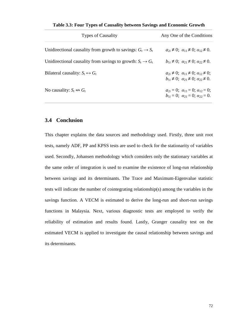
Table 3.3: Four Types of Causality between Savings and Economic Growth .............. 72

Table 4.1: Results of Unit Root Tests ........................................................................... 75

Table 4.2: Results of Johansen Cointegration Test ....................................................... 78

Table 4.3: Normalized Cointegrating Vectors............................................................... 80

Table 4.4: Estimated Long-run and Short-run Domestic Savings Equations Using the VECM Approach.......................................................................................... 84

Table 4.5: Granger Causality Test Results based on VECM ........................................ 89

xii

LIST OF ABBREVIATIONS

ADB Asian Development Bank

ADF Augmented Dickey-Fuller

ADR age dependency ratio

AIC Akaike Information Criterion

ARCH Autoregressive Conditional Heteroscedasticity

ARDL Autoregressive Distributed Lag

BG Breusch-Godfrey

BNM Bank Negara Malaysia

CAB Balance on Current Account

CNLRM Classical Normal Linear Regression Model

DF Dickey-Fuller

DOS Department of Statistics

ECM error correction model

ect error correction term

FCI foreign capital inflows

FDI Foreign Direct Investment

GDP Gross Domestic Product

GDPS Gross Domestic Private Savings

GDS Gross Domestic Savings

GNI Gross National Income

GNP Gross National Product

GNS Gross National Savings

Ha alternative hypothesis

xiii

H0 null hypothesis

I investment expenditure

i.i.d. independently and identically distributed

IMF International Monetary Fund

INT interest rates

JB Jarque-Bera

KPSS Kwiatkowski-Phillips-Schmidt-Shin

LCH Life Cycle Hypothesis

LM Lagrange Multiplier

MDR modified version of dependency ratio

MPS Marginal Propensity to Save

OADR old-age dependency ratio

OECD Organization for Economic Cooperation and Development

OLS Ordinary Least Squares

PDF probability density function

PIH Permanent Income Hypothesis

PP Phillips-Perron

RINT real interest rates

S savings

SBC Schwartz Bayesian Criterion

s.e. standard error

TYDL Toda & Yamamoto and Dolado & Lütkepohl

VAR Vector Autoregression

VECM Vector Error Correction Model

YADR young-age dependency ratio

YD disposable income

xiv

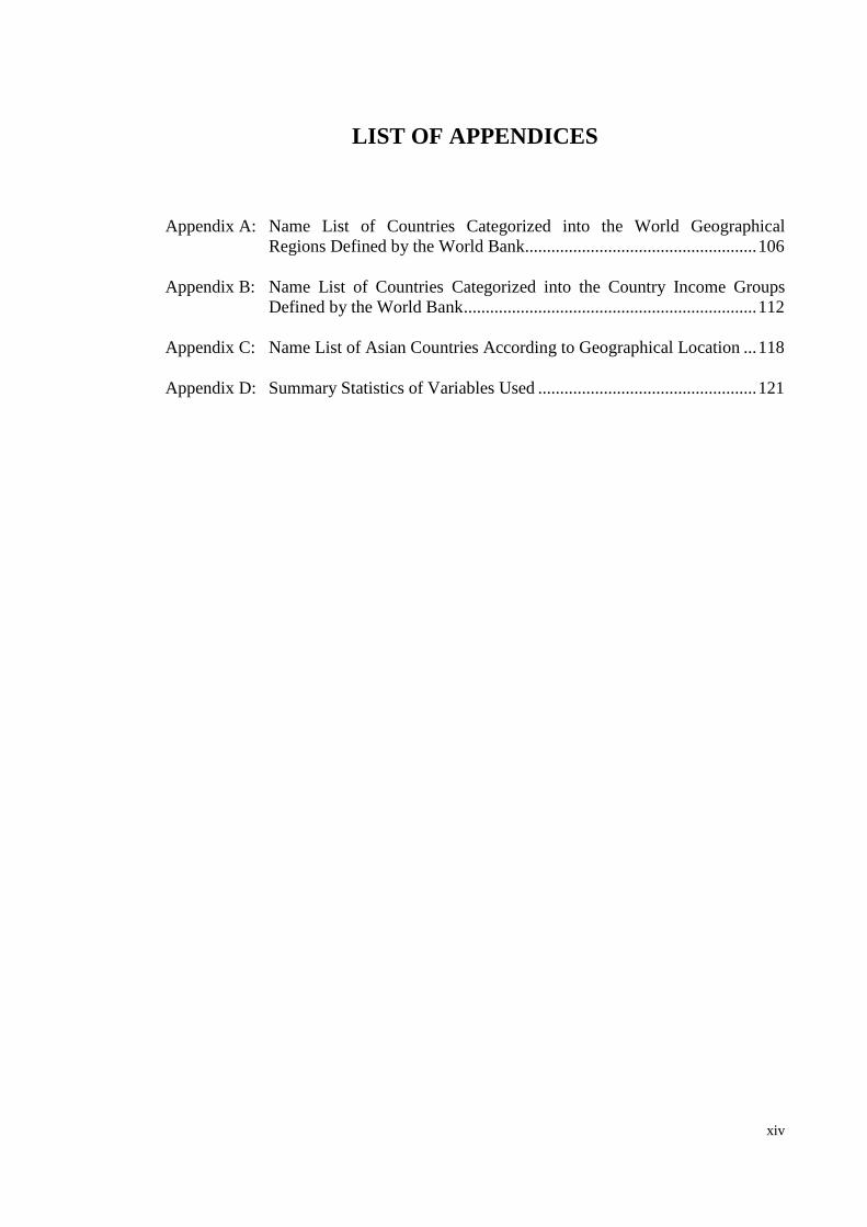
LIST OF APPENDICES

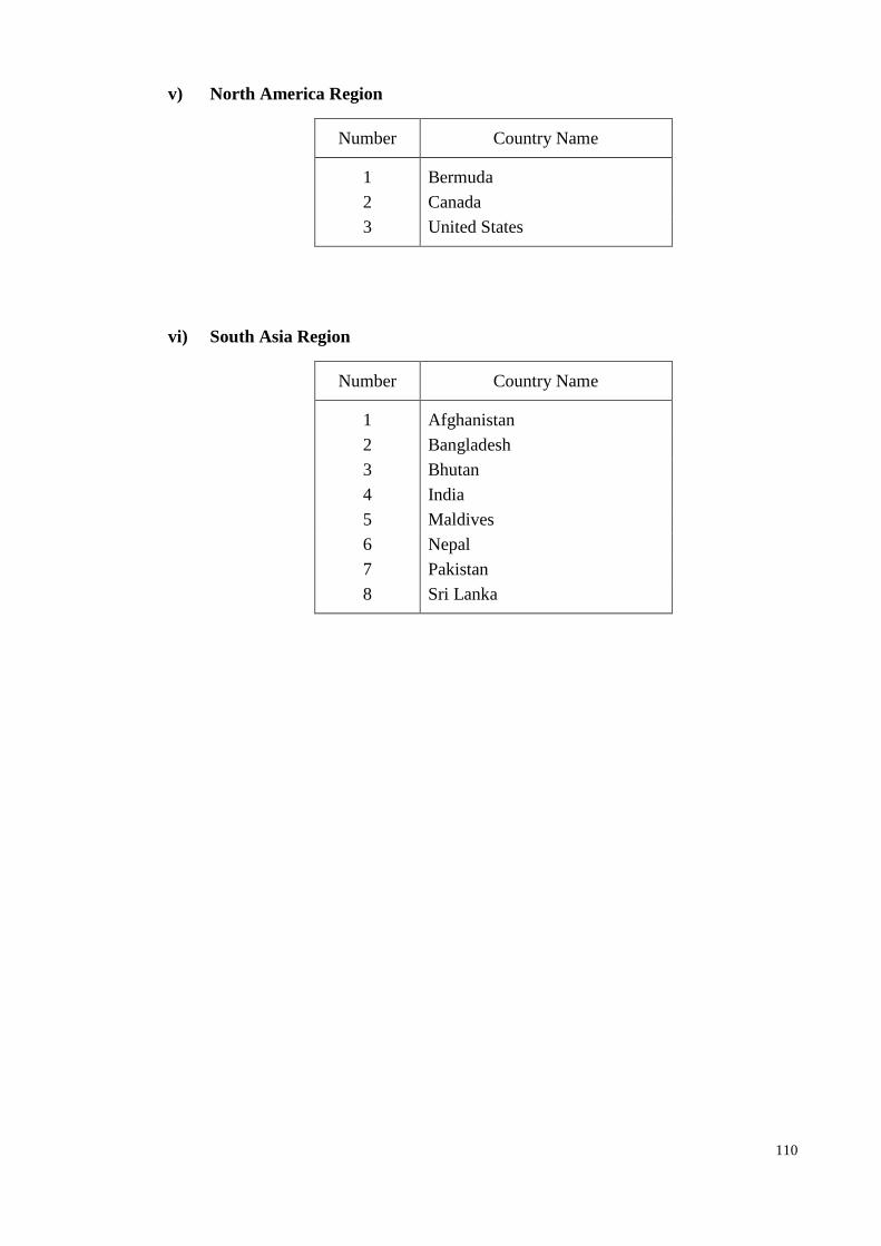
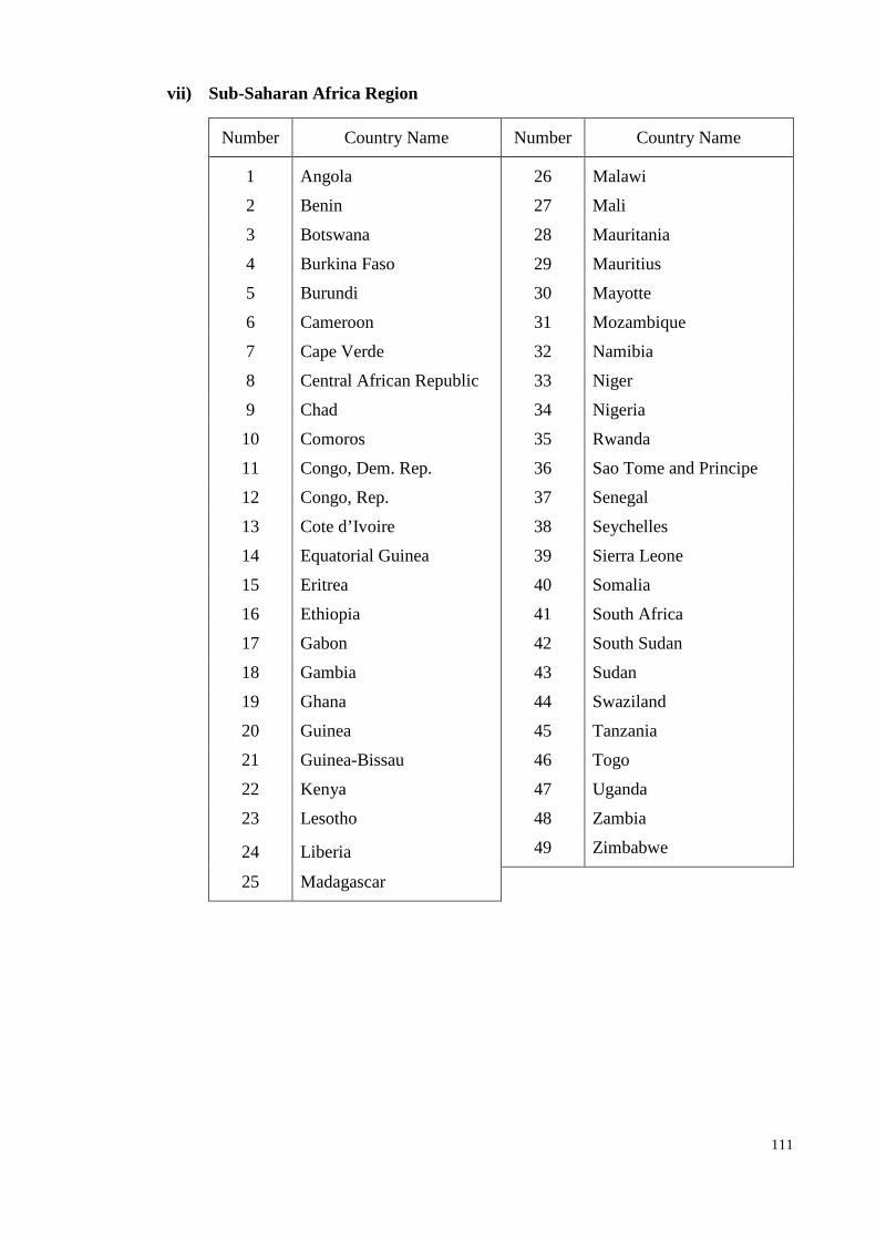
Appendix A: Name List of Countries Categorized into the World Geographical Regions Defined by the World Bank..................................................... 106

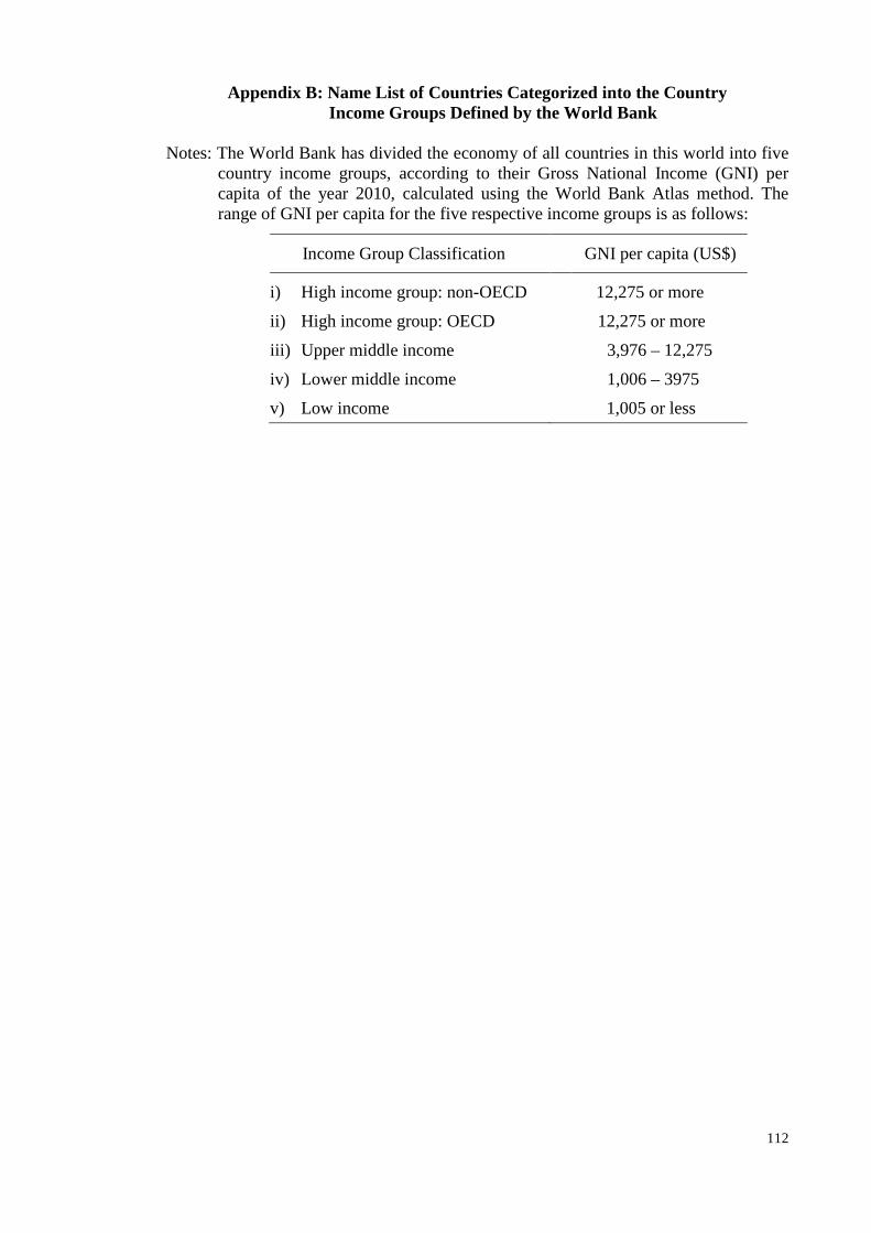
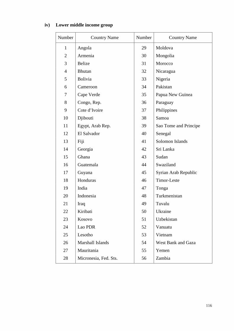
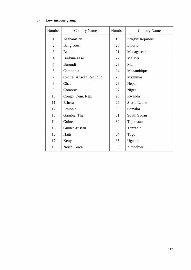
Appendix B: Name List of Countries Categorized into the Country Income Groups Defined by the World Bank ................................................................... 112

Appendix C: Name List of Asian Countries According to Geographical Location ... 118

Appendix D: Summary Statistics of Variables Used .................................................. 121

1

CHAPTER 1 - INTRODUCTION

1.1 Background of the Study

Rapid economic growth is always one of the crucial macroeconomic objectives to be

achieved by every country in this world. This is because of economic growth is one of

the most important determinants for standards of living and quality of life for the people

in a country. Therefore, in the past, there are many studies and research works have

been carried out to explore the factors leading to higher economic growth in a country.

In the process of economic development for a country, high savings rates and

investment rates are needed to ensure its sustained and high rates of economic growth.

This is according to the growth theories for example, proposed by Solow (1956) and

Romer (1986) who stated that higher economic growth in a country can be caused by

high savings rates through the impact on capital formation in the country. However, Lin

(1992) mentioned that economic growth can be sustained only if the resources such as

savings are mobilized efficiently and translated effectively into the productive activities

in the country [cited in Tang (2008)]. Thus, there is a possibility for higher savings rates

to lead to high economic growth provided that the condition of optimal mobilization of

resources is fulfilled.

Asian region had experienced rapid economic growth in the past three decades

especially in the early of 1990s. It has been a focus for many foreign investors by way

of attracting almost half of the capital flows from developed nations. However, the

Asian financial crisis that attacked Thailand in July 1997 and then spread to most of the

Asian countries had changed the scenario stated before this. As a result of the 1997

2

financial crisis, most of the Asian currencies had suffered from sharp depreciation and

thereafter, this triggered a massive outflow of capital from the Asian region. As the

foreign capital is highly mobile in the international markets, it is crucial for every

government to understand the close relationship between national savings and foreign

savings, and then make use of its national savings to develop the economy and not just

rely on foreign savings or capital in this matter.

Based on the World Bank data from 1980s onwards, most of the countries (including

Malaysia) in East Asian and Southeast Asian regions have shown higher savings rates

and economic growth rates compare with other countries in the world. Thus, Malaysia is

suitable to be studied for analysis of relationship between savings and growth in a

country. In fact, this analysis has gained much attention in the theoretical literature and

past empirical research. If high savings can be proven to Granger-cause to high growth

in Malaysia, this empirical finding can be used to explain the relatively higher growth

rates for the East Asian and Southeast Asian countries.

1.2 Savings in Malaysia: An Overview from World Perspective

Despite the declining world’s average savings rate in the past four decades since the

early 1970s throughout the late 2000s, there are few countries in this world which have

consistently achieved and managed to sustain their savings rates to be above 25 percent

of the country’s Gross Domestic Product (GDP) for at least three decades in the past.

By using the World Development Indicators from World Bank as a source, with the cut-

off of an average Gross Domestic Savings (GDS) rate of 25 percent to GDP of a

3

country, Table 1.1 summarizes the high savings countries in the world for the time

period of 1970s to 2000s.

Table 1.1: High Savings Countries in the World, 1970s – 2000s (with percentage of average GDS to GDP > 25%)

Country 1970s 1980s 1990s 2000s

Algeria 35.17 31.49 30.14 49.15 Botswana 21.12 35.27 38.83 36.48 Brunei Darussalam 45.19 35.86 49.90 China 30.42 35.45 41.15 45.82 Congo, Rep. 12.01 31.94 28.82 48.27 Finland 28.34 27.25 24.61 26.82 Gabon 54.29 44.27 43.63 53.28 Hong Kong 30.78 33.67 31.90 31.21 Indonesia 24.97 31.59 30.17 30.46 Iran, Islamic Rep. 33.90 16.80 35.92 39.27 Japan 35.40 31.61 30.57 24.61 South Korea 22.12 30.87 36.30 31.59 Kuwait 59.40 33.07 10.40 43.70 Luxembourg 35.22 30.63 39.81 47.40 Macao 45.99 52.10 60.46 Malaysia 27.10 30.25 40.66 42.23 Netherlands 26.09 24.63 26.89 27.16 Norway 30.50 31.31 28.63 36.31 Oman 50.52 39.70 24.98 43.22 Panama 28.57 27.72 27.15 Russian Federation 34.73 31.48 33.11 Saudi Arabia 59.34 26.46 27.53 43.81 Singapore 29.13 42.39 48.67 47.57 Switzerland 31.00 29.01 28.70 29.42 Thailand 22.26 26.47 35.26 31.64 Trinidad and Tobago 35.27 24.20 27.98 39.61 Turkmenistan 28.08 28.90 42.25 Venezuela 37.82 25.02 26.50 34.50

World as a whole 24.64 22.83 22.51 21.39

Source: Computed from annual data in World Development Indicators 2011, World Bank.

From the total of 216 countries in the World Bank’s 2011 database, 28 countries are

categorized as the consistent high savers, of which 12 of them had shown the average

GDS rate above 25 percent for all the four decades. From the 28 countries, there are ten

4

countries (including Malaysia) come from either East Asian or Southeast Asian region.

Besides, there are only five countries (including Malaysia) which able to achieve an

upward trend for its savings rates throughout the four decades. For instance, the average

GDS rate of Malaysia had increased from 27.10 percent in the 1970s, 30.25 percent in

the 1980s, 40.66 percent in the 1990s, to 42.23 percent of GDP in the 2000s.

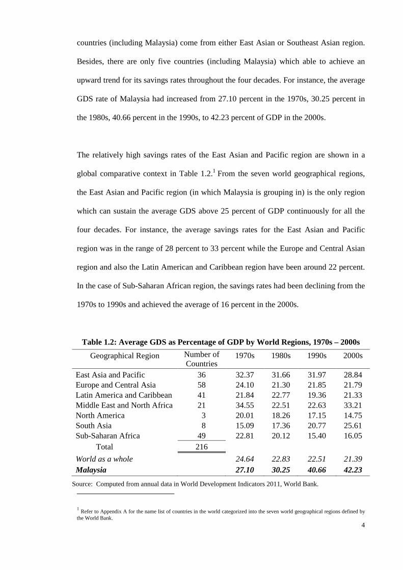
The relatively high savings rates of the East Asian and Pacific region are shown in a

global comparative context in Table 1.2.1 From the seven world geographical regions,

the East Asian and Pacific region (in which Malaysia is grouping in) is the only region

which can sustain the average GDS above 25 percent of GDP continuously for all the

four decades. For instance, the average savings rates for the East Asian and Pacific

region was in the range of 28 percent to 33 percent while the Europe and Central Asian

region and also the Latin American and Caribbean region have been around 22 percent.

In the case of Sub-Saharan African region, the savings rates had been declining from the

1970s to 1990s and achieved the average of 16 percent in the 2000s.

Table 1.2: Average GDS as Percentage of GDP by World Regions, 1970s – 2000s

Geographical Region Number of Countries

1970s 1980s 1990s 2000s

East Asia and Pacific 36 32.37 31.66 31.97 28.84 Europe and Central Asia 58 24.10 21.30 21.85 21.79 Latin America and Caribbean 41 21.84 22.77 19.36 21.33 Middle East and North Africa 21 34.55 22.51 22.63 33.21 North America 3 20.01 18.26 17.15 14.75 South Asia 8 15.09 17.36 20.77 25.61 Sub-Saharan Africa 49 22.81 20.12 15.40 16.05

Total 216

World as a whole 24.64 22.83 22.51 21.39 Malaysia 27.10 30.25 40.66 42.23


1 Refer to Appendix A for the name list of countries in the world categorized into the seven world geographical regions defined by the World Bank.

5

Table 1.3 summarizes the savings rates (share of average GDS in GDP) achieved by the

five country income groups.2 It can be seen that besides the high income: non-OECD

income group, the upper middle income group (in which Malaysia is grouping in) is the

only income group in which the average savings rate was above 25 percent of GDP for

all the four decades since 1970s. Furthermore, the upper middle income group is the

only group which showed an upward trend in the average savings rates for the four

decades (i.e. increased from 25.05 percent in the 1970s to 29.85 percent of GDP in the

2000s).

Table 1.3: Average GDS as Percentage of GDP by Country Income Groups, 1970s – 2000s

Income Group Number of Countries

1970s 1980s 1990s 2000s

High income: non-OECD 39 38.25 33.19 29.99 35.33 High income: OECD 31 24.45 22.07 21.66 19.52 Upper middle income 54 25.05 26.93 27.25 29.85 Lower middle income 56 17.50 18.86 19.76 23.22 Low income 36 7.27 8.26 9.64 10.12

Total 216

World as a whole 24.64 22.83 22.51 21.39

Malaysia 27.10 30.25 40.66 42.23


1.3 Savings in Malaysia: An Overview from Asian Region

The economy of Asian region is one of the most successful regional economies in the

world because this region consists of quite a number of large and prosperous economies

located either in East Asian, Southeast Asian or South Asian region. For examples,

there are China, Hong Kong, Japan, South Korea and Taiwan located in the East Asian

2 Refer to Appendix B for the name list of countries in the world categorized into the five country income groups defined by the World Bank.

6

region. Besides, there are Singapore, Indonesia, Malaysia, Thailand and the rest of eight

countries located in the Southeast Asia.3

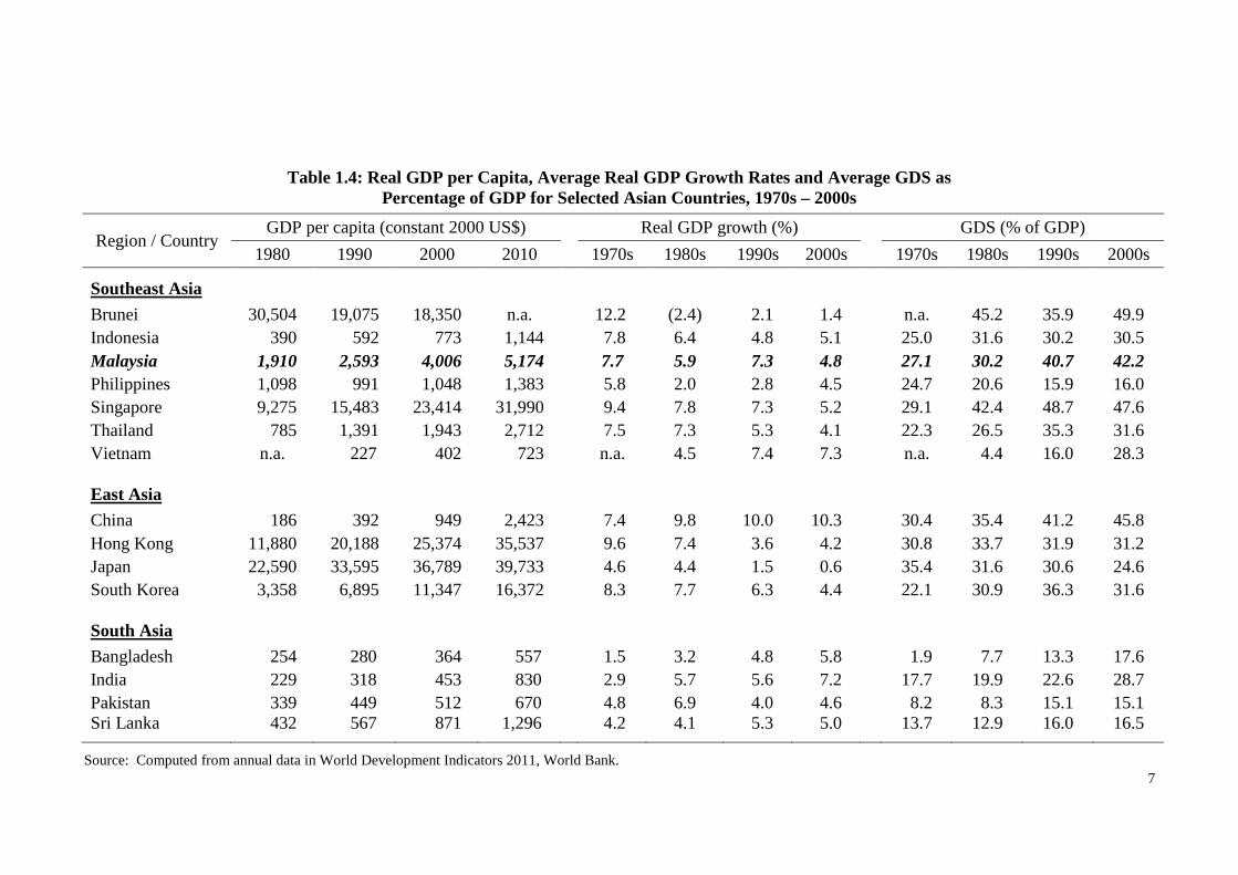
Table 1.4 shows a comparative picture of the Malaysian real GDP per capita (2000 =

100), real GDP growth rates and ratio of GDS to GDP with the corresponding data of

selected Asian countries from Southeast Asia, East Asia and South Asia. It is observed

that in 1980, Malaysia was one of the highest real GDP per capita countries, after

Brunei, Japan, Hong Kong, Singapore and South Korea. This ranking remained

unchanged over the next three decades until 2010.

Besides, real GDP growth rates of Malaysia were averaged at 7.7 percent in the 1970s,

5.9 percent in the 1980s and 7.3 percent in the 1990s, which were above the

performance of many Asian developing countries. Somehow, Malaysian growth rates of

real GDP had declined to average 4.8 percent in the 2000s prior to the global economic

crisis in 2008. Over the three decades from 1970s to 1990s, the average real GDP

growth rate of Malaysia was relatively higher than the Philippines, Japan, Bangladesh,

India and Sri Lanka, but lower than that of the rest of countries listed in the Table 1.4.

In contrast, besides Singapore and China, Malaysia is the only Asian country which has

shown not only high, but at an upward trend for the savings rates where the average

GDS rate was above 25 percent of GDP since the 1970s throughout the four decades.

The savings rate of Malaysia is relatively higher than many other Asian countries in the

world, especially all the South Asian countries and most of the Southeast Asian

countries.

3 Refer to Appendix C for the name list of Asian countries according to six geographical locations, i.e. East Asia, Southeast Asia, South Asia, West Asia, North Asia and Central Asia.

7

Table 1.4: Real GDP per Capita, Average Real GDP Growth Rates and Average GDS as Percentage of GDP for Selected Asian Countries, 1970s – 2000s

Region / Country GDP per capita (constant 2000 US$) Real GDP growth (%) GDS (% of GDP)

1980 1990 2000 2010 1970s 1980s 1990s 2000s 1970s 1980s 1990s 2000s

Southeast Asia

Brunei 30,504 19,075 18,350 n.a. 12.2 (2.4) 2.1 1.4 n.a. 45.2 35.9 49.9 Indonesia 390 592 773 1,144 7.8 6.4 4.8 5.1 25.0 31.6 30.2 30.5 Malaysia 1,910 2,593 4,006 5,174 7.7 5.9 7.3 4.8 27.1 30.2 40.7 42.2 Philippines 1,098 991 1,048 1,383 5.8 2.0 2.8 4.5 24.7 20.6 15.9 16.0 Singapore 9,275 15,483 23,414 31,990 9.4 7.8 7.3 5.2 29.1 42.4 48.7 47.6 Thailand 785 1,391 1,943 2,712 7.5 7.3 5.3 4.1 22.3 26.5 35.3 31.6 Vietnam n.a. 227 402 723 n.a. 4.5 7.4 7.3 n.a. 4.4 16.0 28.3

East Asia

China 186 392 949 2,423 7.4 9.8 10.0 10.3 30.4 35.4 41.2 45.8 Hong Kong 11,880 20,188 25,374 35,537 9.6 7.4 3.6 4.2 30.8 33.7 31.9 31.2 Japan 22,590 33,595 36,789 39,733 4.6 4.4 1.5 0.6 35.4 31.6 30.6 24.6 South Korea 3,358 6,895 11,347 16,372 8.3 7.7 6.3 4.4 22.1 30.9 36.3 31.6

South Asia

Bangladesh 254 280 364 557 1.5 3.2 4.8 5.8 1.9 7.7 13.3 17.6 India 229 318 453 830 2.9 5.7 5.6 7.2 17.7 19.9 22.6 28.7 Pakistan 339 449 512 670 4.8 6.9 4.0 4.6 8.2 8.3 15.1 15.1 Sri Lanka 432 567 871 1,296 4.2 4.1 5.3 5.0 13.7 12.9 16.0 16.5


8

1.4 Savings and Economic Growth Rates in Malaysia

Malaysia can be said as one of the fast-growing economies in the Southeast Asia due to

its high real GDP growth rates, especially from the 1970s to 1990s. Besides, real GDP

per capita of Malaysia is the third highest among the Southeast Asian countries,

followed after Singapore and Brunei (see Table 1.4).

The relatively high economic growth rates in Malaysia are always linked to the

intensive flows of Foreign Direct Investment (FDI) especially in the 1980s and 1990s.

Furthermore, with the rapid expansion of international trades at the same time, this

further aid to the achievement of high economic growth rates. Besides, the relatively

high savings rates could be one of the factors or determinants of high economic growth

in Malaysia since the Malaysian savings rate is the third highest among the Southeast

Asian countries, followed after Singapore and Brunei (see Table 1.4).

Figure 1.1 depicts the GDS rates (as a percentage of GDP) and the real GDP growth

rates in Malaysia from 1970 to 2009. In overall, the savings rate shows an upward trend

in which it had increased from 24.3 percent in 1970 to 36.0 percent in 2009. In 1998,

the savings rate achieved its highest rate in the history, i.e. 48.7 percent. However, it

started to fall dramatically from 1998 to 2002. This could be resulting from the Asian

financial (or currency) crisis which attacked some of the Asian countries (including

Malaysia) from mid of 1997 to end of 1998.

During 2001 to 2008, the savings rates seem to be constant and floated within the range

of 41 to 44 percent of GDP. However, there is a sharp fall again in 2009 where the

savings rate fell from 42.3 percent in 2008 to 36.0 percent in 2009. This could be due to

9

the global financial crisis which was started with the subprime mortgage crisis in the

United States. Despite the dwi-crisis in the 1990s and 2000s, Malaysia is still able to

sustain its high level of savings rate until nowadays.

Figure 1.1: GDS as Percentage of GDP, and Real GDP Growth Rates in Malaysia, 1970 – 2009

Source: World Development Indicators 2011, World Bank.

On the other hand, Malaysian real GDP growth rate shows a constant trend throughout

the period of this study but relatively high economic growth rates among the Southeast

Asian countries, especially from 1988 to 1996 where the growth rates were floated in

the range of 8.9 percent to 10.0 percent. There are four structural breaks in the trend due

to different causes.

In the 1970s, Malaysia had achieved an average annual rate of 7.7 percent for its

economic growth (see Table 1.4). Such a high growth rate was achieved from the result

of significant improvement in the performance of manufacturing sector where this

10

sector managed to grow by an average annual rate of 22.9 percent during 1971–1980

and furthermore contributed to 21.6 percent of Malaysian GDP in 1980 (Ang, 2009).

Besides, Yusof et al. (1994) highlighted that the high growth rates in the 1970s was also

due to the government efforts where the government had aggressively promoting its

export-oriented industries through the establishment of free trade zones since early of

the 1970s [cited in Ang (2009)]. As a result, Malaysia enjoys a success in export-

oriented and labor-intensive industries, for examples, textiles, electronics and wool

products.

However, there was the first time for the Malaysian growth rate to fall sharply from 8.3

percent in 1974 to only 0.8 percent in 1975 due to the oil crisis which had led to the

world recession in 1975. The Malaysian government had responded to the crisis by

increasing government spending largely on public investment projects (Ang, 2009). As

a result, the growth rate of real GDP started to increase and achieved 11.6 percent

(which was also the second highest growth rate in the past decades) in 1976.

In the 1980s, Malaysian average annual rate of growth was 5.9 percent (see Table 1.4),

slightly lower than the previous decade. According to Ang (2009), this relatively lower

growth rate was mainly caused by two reasons. Firstly, there was a prolonged global

economic recession in the early 1980s caused to a dramatic fall in commodity prices.

Secondly, the collapse of several main export commodity prices in 1985 had led to the

economic recession again. Figure 1.1 shows that the real GDP growth rate in 1985 was

–1.1 percent (the first time for Malaysian growth rate to be negative). However, the

economy started to recover and managed to achieve and sustain an annual growth of 9.0

to 10.0 percent from 1988 to 1996, as a result of external conditions which led to a

spectacular performance in the export sector during 1988–1990, active contribution of

11

private sector in developing the economy and furthermore, the massive increase of FDI

into Malaysia during 1991–1996 (Ang, 2009).

As shown in Figure 1.1, there was another and also the most serious breakpoint

occurred in 1998 as the outcome of the Asian financial crisis started in mid of 1997. In

1998, Malaysian real GDP growth rate had recorded the lowest rate in the four decades,

i.e. –7.4 percent. However, Malaysian economy had recovered from the crisis and

achieved the growth rate within the range of 5.3 to 8.9 percent for 1999–2007, with the

exception of year 2001. The growth rate was only 0.5 percent in 2001 due to the world

trade recession (Ang, 2009). Lastly, Malaysia recorded –1.7 percent for the growth rate

in 2009 due to the global economic crisis in 2008.

1.5 Statement of Research Problem

Since the 1980s, there are many research publications which discussed about the high

economic achievements among most of the Asian countries such as China, Hong Kong,

Singapore, Taiwan, South Korea, Malaysia, Indonesia and Thailand. The databank of

World Bank had revealed that the average annual growth rate of GDP for these

countries was two times higher as compared to other developing countries in the same

region.

The Malaysian economy is focused in this study because Malaysia exhibits among the

higher savings and growth rates in the Southeast Asian region. Thus, Malaysia is

particularly suitable to be used for an analysis of the relationship between savings and

economic growth in a country. Besides that, the direction of causation between savings

and growth will be investigated in this study as well.

12

The empirical findings and evidence found from the previous research works are still

unclear and ambiguous about the relationship between savings and its determinants, and

also the direction of causation between savings and growth in a country. Furthermore,

the empirical works have derived different results and conclusions subject to the

country and time period used in the study.

In this study, the determinants of savings in Malaysia will be examined and Granger

causality between savings and its determinants (especially economic growth) in

Malaysia will be analyzed.

1.6 Significance of the Study

From the previous studies and research, savings in a country is found to be significant

and closely related to its economic growth. This makes our study on savings behavior in

Malaysia and the causality between its savings and growth become crucial and

meaningful. However, there are not many studies being carried out in the past to study

about this matter for the case of Malaysia. Thus, the present study will be able to fill the

gap and to complement the previous studies.

In this study, a comprehensive set of data using domestic data statistics, together with

some other relevant explanatory variables which are expected to be the main

determinants of savings in Malaysia will be used. This study also provides an estimated

long-run domestic savings equation over a relatively longer time period than most of the

previous studies on Malaysia.

13

The study conducted is important to the policymakers of Malaysia because the results

obtained will be useful for macroeconomic analysis. Malaysian government has to

ensure that the economy can sustain high economic growth rates in the forthcoming

decades in order for Malaysia to become a developed and high-income nation, as

proposed by the seventh Prime Minister, Dato’ Sri Mohd Najib bin Tun Abdul Razak in

the year of 2010.

If savings is proved to be a factor Granger cause to high economic growth in the

country, one of the main goals and objectives of government policies set by the

government is to encourage savings. In contrast, if growth results less from savings but

more from other factors such as human capital, technological innovation and

advancement, and trade policy, the government can set these targets for the government

policies.

1.7 Objectives of the Study

In general, this study attempts to study empirically the relationship between savings and

economic growth in Malaysia using a relatively longer time period from 1970 to 2010.

Following from this, the specific objectives of the study are:

i) To examine the relationship between savings and its determinants in Malaysia in

both short run and long run.

ii) To investigate the direction of causality between savings and its determinants

(especially economic growth).

14

1.8 Research Organization

This study consists of five chapters. Chapter one provides an introduction and

illustration for the statement of research problem, significance and objectives of the

study. The savings and growth in various countries around the world and the relative

performance of Asian countries including Malaysia are discussed briefly.

Chapter two reviews the determinants of savings and provides certain definitions of

how these variables are measured. This chapter also reviews the extant empirical

literature on savings model across many dimensions and countries.

Chapter three highlights the sources of data used. In addition, the research methodology

about econometric procedures used to estimate the savings function in Malaysia and the

analysis for direction of causality between savings and growth will be explored.

Chapter four presents and discusses the empirical results obtained from the study.

Chapter five concludes the thesis with a review of the main findings of the study and

highlights some implications that arise from them. The chapter also discusses the

limitations of the study and identifies issues for future research.

15

CHAPTER 2 - LITERATURE REVIEW

2.1 Introduction

In the previous chapter, an overview about savings and economic growth rates in

Malaysia, statement of research problem, significance and objectives of the study have

been presented. In this chapter, Section 2.3 reviews the determinants of savings. Review

of the literature related to the causality between savings and economic growth will be

presented in Section 2.4.

2.2 Theoretical Framework

Based on the objectives of the study, a theoretical framework showing the relationship

among the variables used in this study was constructed and depicted by Figure 2.1. The

study attempts to identify the determinants of savings in Malaysia. Besides, direction of

causality between savings and its determinants will be examined too.

Figure 2.1: Theoretical Framework Describing the Relationship between All Variables Used in the Study

A multivariate model will be used to estimate the savings function as follows.

LRGDSt = α0 + β1LRGDPt + β2LADRt + β3INTt + β4CABt + εt ................ (2.1)

where L denotes natural logarithm (ln)

Gross Domestic Product (GDP) Interest Rates (INT)

Age Dependency Ratio (ADR)

)

Gross Domestic Savings (GDS) Balance on Current

Account (CAB)

16

RGDS is real Gross Domestic Savings

RGDP is real Gross Domestic Product

ADR is age dependency ratio

INT is interest rates

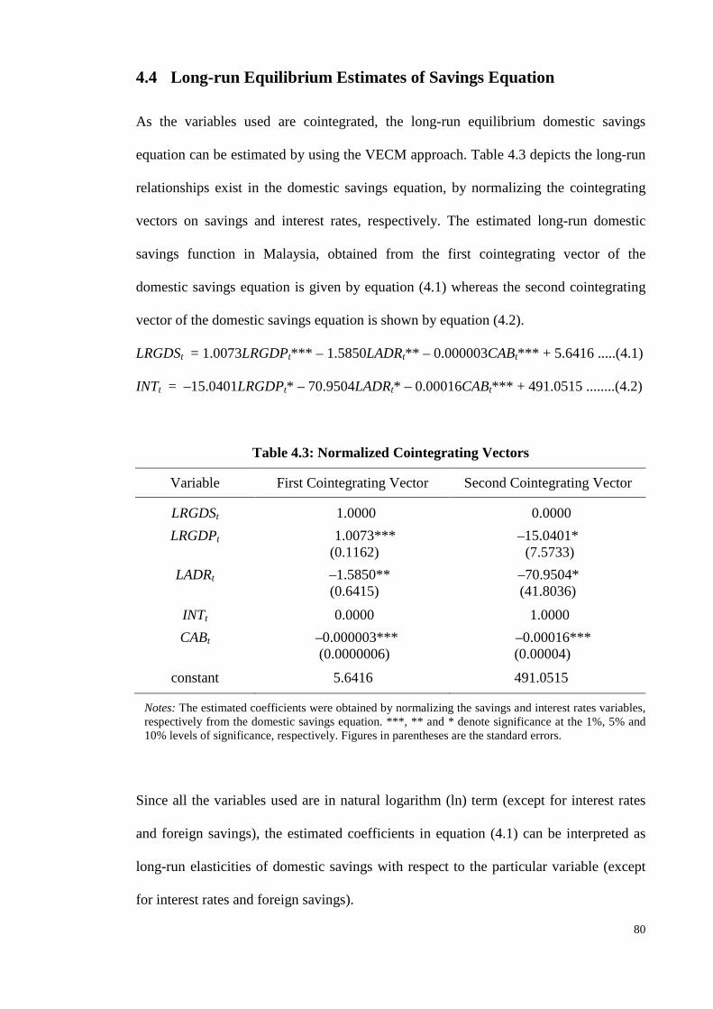
CAB is Balance on Current Account (as a proxy for foreign savings)

α0 is the intercept parameter

β1, β2, β3 and β4 are the slope coefficients

εt is the error term which is assumed to be white noise and in normal distribution

(with zero mean and constant variance)

2.2.1 Operational Definition of Variables

A set of definition and brief notes for the variables used is as follows. These definitions

are widely used and taken mostly from the source of Department of Statistics (DOS),

Malaysia, Bank Negara Malaysia (BNM) and International Monetary Fund (IMF).

Gross Domestic Savings (GDS) refer to the difference between GDP and total

consumption, where total consumption is the sum of private consumption and

government consumption. In this study, GDS is derived by subtracting final

consumption expenditure from GDP at purchasers’ value.

Gross Domestic Product (GDP) refer to the total value of producing all final goods and

services in a country within a calendar year, before deducting allowances for

consumption of fixed capital. GDP can be measured in three but equivalent ways, i.e.

the sum of value added, sum of final expenditures and sum of incomes. GDP based on

expenditure approach, i.e. the total final expenditure at purchasers’ values, subtract the

free on board (f.o.b.) value of imports of goods and services is used in this study.

17

Age Dependency Ratio (ADR) is the ratio of unproductive or non-working age

population (below 15 and above 65 years old) to the productive or working age

population (15 to 64 years old).

Interest rates (INT) used in this study is proxy by the fixed deposit interest rates which

refer to the average fixed deposit rates of commercial banks, finance companies and

merchant banks for maturities of 12 months.

Balance on Current Account (CAB) is the sum of the sub-components balance on

goods, services, income, and net current transfers. Current account (which is one of the

accounts in the Balance of Payments) records all transactions other than those in

financial and capital items. CAB is used as a proxy for foreign savings in this study.

2.3 Determinants of Savings

In general, the more significant and common determinants of savings found from the

literature review are economic growth, dependency ratio, interest rates and foreign

savings.

2.3.1 Economic Growth

The concept of a simple savings function was first explained by John Maynard Keynes

in the early of 1930s under his demand-determined model of output and employment.

(Begg, Fisher, & Dornbusch, 2003). According to Keynes, the simplified savings

function is given as

S = – a + (1 – b)YD ............................................. (2.2)

18

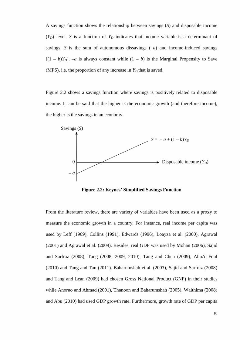
A savings function shows the relationship between savings (S) and disposable income

(YD) level. S is a function of YD indicates that income variable is a determinant of

savings. S is the sum of autonomous dissavings (–a) and income-induced savings

[(1 – b)YD]. –a is always constant while (1 – b) is the Marginal Propensity to Save

(MPS), i.e. the proportion of any increase in YD that is saved.

Figure 2.2 shows a savings function where savings is positively related to disposable

income. It can be said that the higher is the economic growth (and therefore income),

the higher is the savings in an economy.

Savings (S)

S = – a + (1 – b)YD

0 Disposable income (YD)

– a

Figure 2.2: Keynes’ Simplified Savings Function

From the literature review, there are variety of variables have been used as a proxy to

measure the economic growth in a country. For instance, real income per capita was

used by Leff (1969), Collins (1991), Edwards (1996), Loayza et al. (2000), Agrawal

(2001) and Agrawal et al. (2009). Besides, real GDP was used by Mohan (2006), Sajid

and Sarfraz (2008), Tang (2008, 2009, 2010), Tang and Chua (2009), AbuAl-Foul

(2010) and Tang and Tan (2011). Baharumshah et al. (2003), Sajid and Sarfraz (2008)

and Tang and Lean (2009) had chosen Gross National Product (GNP) in their studies

while Anoruo and Ahmad (2001), Thanoon and Baharumshah (2005), Waithima (2008)

and Abu (2010) had used GDP growth rate. Furthermore, growth rate of GDP per capita

19

was used by Edwards (1996), Attanasio et al. (2000) and Agrawal et al. (2009).

Similarly, growth rate of GNP per capita was used by Agrawal (2001) while growth rate

of income per capita was used by Deaton and Paxson (1997), Faruqee and Husain

(1998) and Ang (2008). From the empirical testing, there is a positive coefficient of

growth found in the savings function from almost all the studies done, irrespective of

which variable is used as the proxy for growth. In this study, real GDP is used to

measure the economic growth rate.

The relationship between savings and economic growth will be further discussed in

Section 2.4.

2.3.2 Dependency Ratio

Besides economic growth, dependency ratio is also an important explanatory variable in

influencing the savings. There were many researchers who have been tried to study the

relationship between savings and demographic factor of a country or region, such as

Leff (1969), Hamid and Kanbur (1993), Edwards (1996), Muradoglu and Taskin (1996),

Faruqee and Husain (1998), Loayza et al. (2000), Agrawal (2001), Baharumshah et al.

(2003), Thanoon and Baharumshah (2005), Ang (2008), Tang (2008), Agrawal et al.

(2009), Tang and Tan (2011) and many more. In understanding the relationship between

these two variables, the Life Cycle Hypothesis (LCH) proposed by Modigliani (1970)

plays an essential role here. The LCH is a theory explaining consumption (and therefore

savings) behavior according to an individual’s position in the life cycle.

The LCH states that besides affected by income growth and population growth, savings

in a country affected by the population age structure (or dependency ratio) as well.

Dependency ratio is defined as the ratio of non-working age population to the working

20

age population. It was noted that the non-productive population, which refers to the

young (i.e. below 15 years old) and elderly or retired group (i.e. 65 years old and above)

tend to have dissavings or negative savings, while there will be positive savings for

those who are during their productive or working years (i.e. 15 - 64 years old).

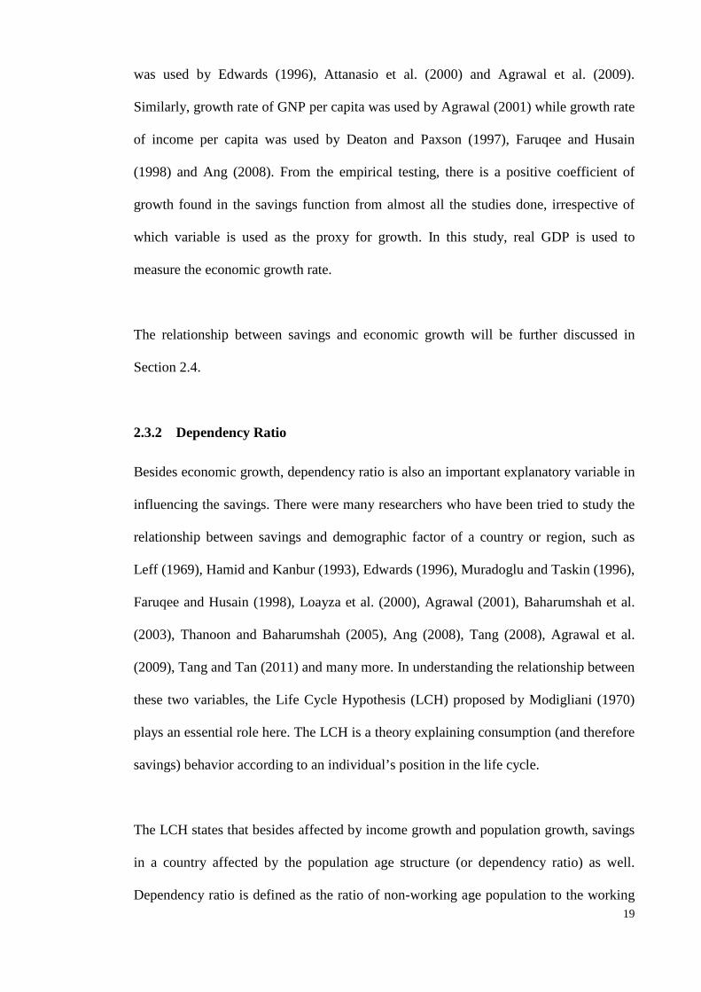
According to the LCH, individuals will have dissavings when they are young, have zero

or low income. During the productive or working years, they will manage to save as the

income earned is higher than the consumption spending. Thus, they will start to

accumulate savings. However, the savings will become negative again when they are

old or have retired. This results in a hump-shaped savings profile over the lifetime of an

individual, as shown by Figure 2.3.

Income, Consumption

savings

consumption

dissavings dissavings

income

0 Time (or stage of life cycle) young working years old or retired

Figure 2.3: Income and Consumption Age Profiles Corresponding Savings over the Household Life Cycle

Source: modified from Mason (1988).

21

It was noted that consumption and income vary in response to the changing

demographic characteristics of the household. However, the proportionate change in

consumption is always smaller than the proportionate change in income due to the

pension motive of households as they have to continue to spend (by using their savings

during the working years) after their retirement (Mason, 1988).

In conclusion, savings rate will be higher if the dependency ratio is lower (meaning a

larger working population relative to the non-working population). Furthermore,

declining fertility rate and smaller aging population will help to increase savings rate of

a country as well. Thus, according to Lahiri (1989), Loayza et al. (2000), Agrawal

(2001) and Agrawal et al. (2009), the sign of estimated coefficient of dependency ratio

in a savings equation is expected to be negative.

Mason (1988) was in opinion that in looking at the relationship between aggregate

savings and population growth rate of a country, it depends on the relative strength

between the dependency effect (which states that rapid population growth discourages

savings) and the rate of growth effect (i.e. rapid population growth encourages savings).

In the context of a household, savings by a household can be influenced by the number

of children in the household. It is logical to say that the higher is the number of children,

the higher is the household consumption spending and thus, the lower is the savings.

There is an inverse relationship between dependency ratio and savings in a household.

However, according to Fry (1994), household with more children may tend to have

higher savings due to the positive bequest motive. There is a possibility to have positive

relationship between savings and dependency ratio in this case. Thus, we can conclude

that the effect of dependency ratio on savings is ambiguous.

22

From the previous empirical studies, it was found that the influence of dependency ratio

on savings can be positive or negative and it varies according to country and time frame

used. However, most of the empirical studies found a negative effect of dependency

ratio on savings. For instance, Leff (1969), Hamid and Kanbur (1993), Agrawal (2001),

Thanoon and Baharumshah (2005) and Tang and Tan (2011) found a negative

coefficient of dependency ratio in the Malaysian savings equation. In other words, there

is an inverse relationship between dependency ratio and savings in Malaysia.

Besides, Rossi (1989) in her study on developing countries found a significant negative

effect of dependency ratio on savings rate. Similarly, Loayza et al. (2000) agreed that an

increase in the young-age dependency ratio (YADR) and old-age dependency ratio

(OADR) tend to reduce the private savings rate in which this is in line with the LCH.

They pointed out that private savings rates will fall about 1 percentage point as the

YADR rises by 3.5 percentage points. Furthermore, the negative impact on savings is

double-up if the OADR increases. In opposite, a country with declining YADR may

enjoy the increases in savings rate in the short run. However, this savings rate will start

to fall when the country faces increasing OADR in the next stage of demographic

maturity. China is an example to explain this scenario. It was noticed that the age

structure is likely to change as a country develops.

Edwards (1996) in his study on 36 Latin American countries for period 1970–1992 and

Agrawal et al. (2009) in their study on five South African countries also found

significant negative result for almost all countries involved in their respective studies.

Agrawal et al. commented that one of the factors for the increasing rates of savings in

South Asia is due to the declining dependency rates.

23

Conversely, the empirical studies which found a significant positive coefficient of

dependency ratio include Fry (1994), Faruqee and Husain (1998), Baharumshah et al.

(2003) and Tang (2008). Baharumshah et al. argued that the positive coefficient found

for ADR could be due to the desire to leave a larger bequest for the dependent as the

dependent ratio in a household become larger. Tang further commented that this

scenario may occur due to the existence of precautionary savings behavior in Malaysia.

Nevertheless, there are empirical studies which found that dependency ratio does not

play any significant role in explaining the savings behavior of a country, such as the

study on savings in the low income per capita countries by Gupta (1971) and the study

on growth, demographic structure and national savings in Taiwan by Deaton and

Paxson (2000b). Deaton and Paxson stated that there is no overall correlation between

age structure and savings rates in Taiwan and thus, the life cycle model cannot be used

to explain about the savings rate.

In conclusion, the effect of dependency ratio on savings is ambiguous and mixed. Thus,

empirical study on Malaysia can be done to re-examine this relation using longer span

of data set.

From the literature review done, instead of using ADR as one of the explanatory

variables, Tang (2008) and Tang and Chua (2012) had proposed and used a new self-

designed variable, i.e. modified version of dependency ratio (MDR). MDR is measured

as the ratio of total unemployed labor force and non-labor force to the total population

of a country. Tang argued that ADR has ignored the existence of unemployed labor

force who is also a dissavings population in a country.

24

ADR is the most appropriate proxy and commonly used as an explanatory variable in a

savings equation to capture the influence of demographic factor to the savings in a

country. In contrast, other proxy measures such as MDR is not a common proxy as it

had been used only by Tang (2008) and Tang and Chua (2012). Besides, Agrawal

(2001) pointed out that the share of labor force or number of employed in total

population is also not appropriate to be used as proxy due to the incomplete data

collection on those self-employed and also labor who are working in the informal

sectors and rural areas. Horioka (1997) mentioned that it is possible and necessary to

segregate the ADR into YADR and OADR since these two ratios may further explain

the savings behavior in a country [cited in Ang (2008)]. However, from the literature

review, YADR and OADR are not frequently to be used in a study. Thus, ADR will be

used in our study as one of the explanatory variables.

2.3.3 Interest Rates

In layman’s term, interest refers the reward to a person who saves money in a financial

institution. The higher is the interest rates, the higher will be the savings. Besides,

interest rates can be the cost of capital paid by a borrower for the use of money

borrowed from a lender as well. The higher is the interest rates, the higher is the cost of

borrowing money and thus, the lower the investment (I) firms will tend to make.

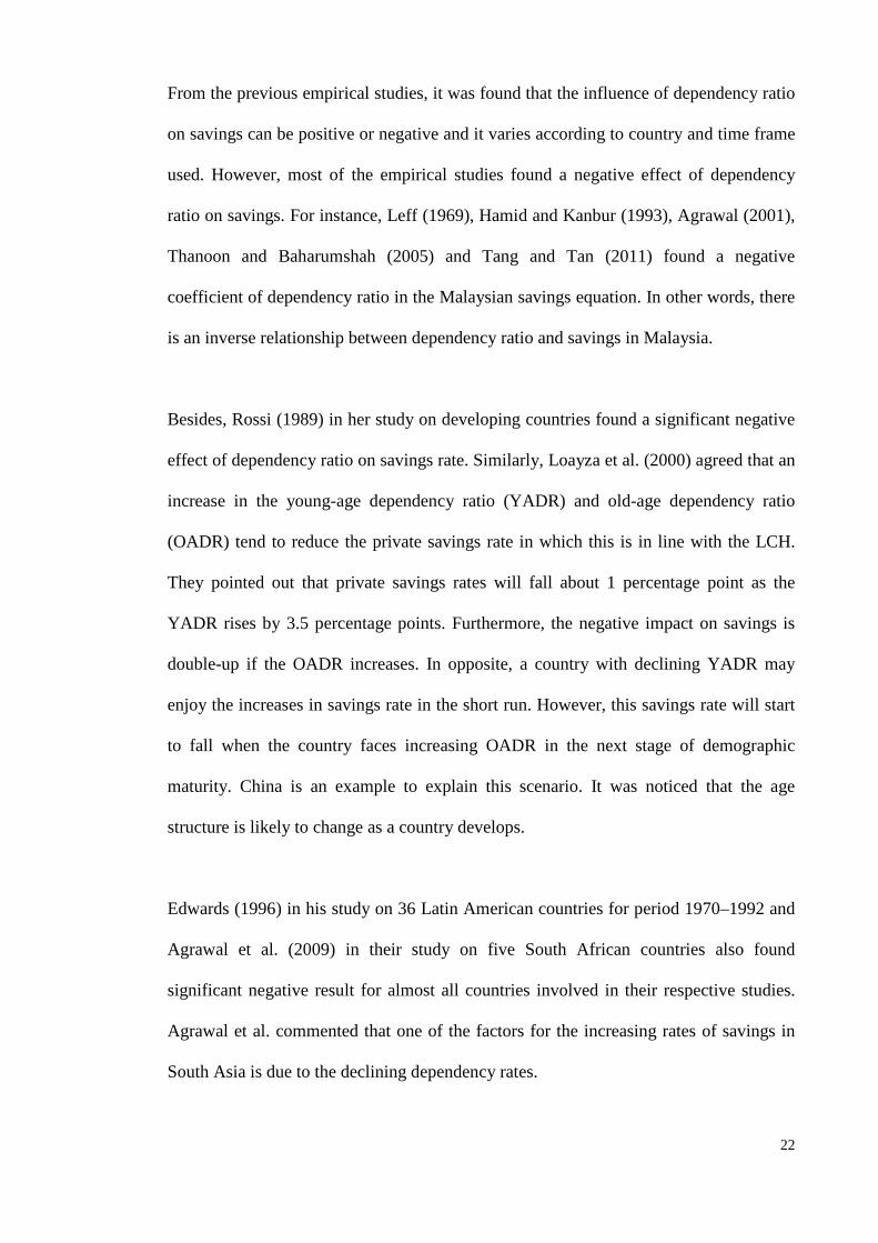
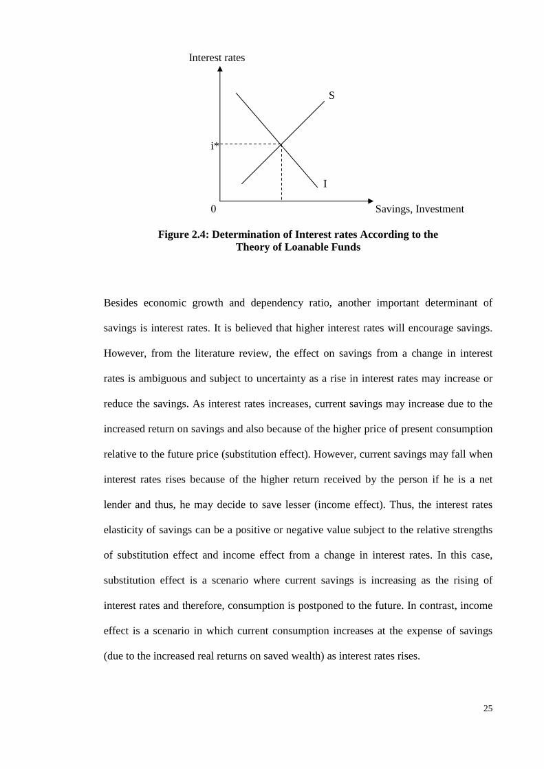
According to the theory of loanable funds supported by the monetarists, interest rate is

determined by demand for and supply of loanable funds, which are the funds available

to borrowers and are generally supplied by banks and other financial institutions. The

determination of interest rates according to this theory is shown by Figure 2.4.

25

Interest rates

S

i*

I

0 Savings, Investment

Figure 2.4: Determination of Interest rates According to the Theory of Loanable Funds

Besides economic growth and dependency ratio, another important determinant of

savings is interest rates. It is believed that higher interest rates will encourage savings.

However, from the literature review, the effect on savings from a change in interest

rates is ambiguous and subject to uncertainty as a rise in interest rates may increase or

reduce the savings. As interest rates increases, current savings may increase due to the

increased return on savings and also because of the higher price of present consumption

relative to the future price (substitution effect). However, current savings may fall when

interest rates rises because of the higher return received by the person if he is a net

lender and thus, he may decide to save lesser (income effect). Thus, the interest rates

elasticity of savings can be a positive or negative value subject to the relative strengths

of substitution effect and income effect from a change in interest rates. In this case,

substitution effect is a scenario where current savings is increasing as the rising of

interest rates and therefore, consumption is postponed to the future. In contrast, income

effect is a scenario in which current consumption increases at the expense of savings

(due to the increased real returns on saved wealth) as interest rates rises.

26

In conclusion, an increase in interest rates will increase the savings if the substitution

effect outweighs the income effect, and vice versa. The net effect of interest rates on

savings depends on the offset from the two effects.

Raut and Virmani (1989) had examined the determinants of consumption and savings

using data from 23 developing countries. They found that despite the real interest rates

has a positive effect on consumption (meaning a negative effect on savings), the

nominal interest rates and inflation rates have negative effects on consumption

(meaning positive effects on savings) where the effect of inflation is significantly

greater than the effect of the nominal interest rates because of the uncertainty arises

from higher inflation.

Empirical past studies had derived different results for the effect of interest rates on

savings in different countries. For examples, by using seven Asian countries, Agrawal

(2001) found a positive coefficient of real interest rates for Thailand and Malaysia, a

negative coefficient for Indonesia, and insignificant coefficient for Singapore, Korea,

Taiwan and India. Besides, Baharumshah et al. (2003) had studied on the savings

dynamics in five of the fast growing Asian countries. The interest coefficient was found

to be positive and significant for Singapore and Korea, negative but insignificant for

Thailand, and positive but insignificant for Malaysia. Thanoon and Baharumshah

(2005) in their study on five Asian countries (including Malaysia) realized that the real

interest rates has a small negative effect on savings, for both short run and long run.

Waithima (2008) found a positive but insignificant coefficient in the private savings

function for Kenya for the period of 1960–2005. From the studies on savings behavior

in five South Asian countries, Agrawal et al. (2009) found a positive and significant

27

coefficient for Bangladesh and Nepal, negative and significant coefficient for India and

Pakistan, but insignificant coefficient for Sri Lanka. The coefficients found are

relatively low for these South Asian countries except for Bangladesh.

The recent empirical studies on Malaysian savings behavior which include the re-

investigation on the influence of interest rates on savings in Malaysia were done by

Tang (2008) and Tang and Tan (2011). By using annual data from 1970 to 2004, Tang

found that the coefficient of real interest rates in real GDS function is negative and

significant in the short run, but is positive and insignificant in the long run. The effect of

real interest rates on Malaysian savings is small as the coefficients were only 0.006 and

0.011 for short run and long run respectively. Lastly, from the study by Tang and Tan

on seven East Asian countries, the long-run coefficient of real interest rates was

negative for China, Hong Kong and Japan while positive for Indonesia, Malaysia, South

Korea and Thailand using the quarterly data from 1970 to 2008.

In overall, it can be concluded that interest rates plays a significant role in affecting the

savings only in certain countries. Besides, the mathematical sign for the estimated

coefficient of interest rates remains ambiguous and it can be varied from country to

country. Nevertheless, from the previous studies, the interest rates was found to have

little impact on savings rate in Malaysia in the long run.

2.3.4 Foreign Savings

In the concept of national income accounting, by definition, the savings-investment

identity states that the amount saved in an economy will be the amount invested in that

economy as well. For an open economy, the total amount saved (i.e. the total of private

savings and foreign savings) must be equal to the total amount invested (i.e. the total of

28

private investment and government borrowing). Hence, investment in an economy will

be financed by private domestic savings, government savings (refer to budget surplus)

and foreign savings (or known as foreign capital inflows). In this scenario, domestic

savings and foreign savings (or capital) can be either complements or substitutes to each

other in financing the investment in an economy.

In the process of economic growth and development, external resources which include

foreign capital flows play a crucial role either as complement to or substitute for

domestic savings in the country, especially to the underdeveloped and developing

countries. Chenery and Elkington (1979) stated that national savings and foreign

savings are complements in the short run but substitutes in the long run [cited in Tan

(2004)]. Thus, these two forms of savings can be in positive or negative relationship.

In the past decades especially the 1990s, the rapid growing Asian countries rely heavily

on foreign capital flows in financing the investment in the country. In looking for the

determinants of savings in Malaysia, foreign savings should be taken into consideration

as one of the explanatory variables since it is a commonly used variable. Furthermore,

the study will be able to examine whether the foreign savings crowded out the savings

in Malaysia. The slope coefficient of foreign savings in the savings equation is the

measurement for the degree of substitutability between foreign savings and domestic

savings (Edwards, 1996; Thanoon & Baharumshah, 2005). Foreign savings will have

negative effect on domestic savings if the foreign savings crowd out domestic savings.

Hamid and Kanbur (1993), Agrawal (2001), Thanoon and Baharumshah (2005) and

Agrawal et al. (2009) stated that greater availability of foreign savings which will

increase the supply of resources in a country may increase consumption spending and

29

thus, lead to a lower national savings. In this case, foreign savings and national savings

are likely to be substitutes and a negative estimated coefficient of foreign savings

should be found in the savings equation.

In fact, in the study of Agrawal (2001) and Baharumshah et al. (2003) using Malaysian

data, foreign savings was found to have a significant negative impact on national

savings. Agrawal et al. (2009) again found that foreign savings rate has a significant

negative impact on domestic savings rate in South Asia (e.g. India, Sri Lanka and

Nepal).

By using annual data from 1970 to 1990, Hamid and Kanbur (1993) found a significant

positive relationship between national savings and foreign savings in Malaysia. They

explained that although there is an inflow of capital, foreign savings do not substitute

domestic savings since the level of national savings is still high in Malaysia. Thanoon

and Baharumshah (2005) also found a significant positive coefficient of foreign savings

in their domestic savings model when they studied the determinants of savings rate in

five Asian countries (including Malaysia) for the 1970–2000 period.

By using a trivariate causality model, Odhiambo (2009) conducted a study which

incorporate foreign capital inflows to examine the direction of causality between

savings and economic growth in South Africa for the period 1950–2005. He was in

opinion that with a low domestic savings rate, in order to sustain a 6 percent of GDP

growth, the country will need to sustain the level of foreign capital inflows. His study

found bidirectional causality between foreign capital inflow and savings in which the

economic growth Granger causes the foreign capital inflow.

30

In conclusion, the previous studies attempted to establish the relationship between

national savings (or domestic savings) and foreign savings failed to reach to an

agreement for the empirical findings whereby the sign for the coefficient of foreign

savings remains ambiguous. It is of interesting to re-examine the above stated relation

using longer span of Malaysian data. In this study, Current Account Balance (CAB) as

the broadest measure of foreign savings (or capital inflows) will be used.

2.4 Causality between Savings and Economic Growth

Besides determine the factors affecting savings in a country, the direction of causality

between savings and its determinants (especially economic growth) is also important to

be examined as the empirical findings may help the government in carrying out the

appropriate development policies.

Generally, there is existence of four types of causality between savings and economic

growth in which the first two types refer to the unidirectional causality either from

savings to growth, or vice versa due to the controversy among two leading schools of

thought. The causality from savings to growth is supported by the “growth theorists”

who assume that savings are invested and translated to growth through effect on capital

accumulation or investment (see Section 2.4.1 for details) whereas the “consumption

theorists” argued that the level and growth of income determine consumption (and

therefore, savings), thus growth leads to savings (see Section 2.4.2 for details).

According to the modern savings theory, there is bidirectional causality where growth

and savings Granger cause each other (see Section 2.4.3 for details). In contrast, there

are cases to certain countries where there is no significant relationship and causality

exists between the savings and growth (see Section 2.4.4 for details).

31

2.4.1 Standard Growth Models

In the past history, there were many economists and researchers attempted to look for

the reasons leading to high economic growth of a country. In general, savings in a

country is found to be one of the main factors leading to economic growth in the

country. In this case, these economists and researchers support the capital

fundamentalists’ point of view that capital formation and accumulation through savings

is the main driving force for high growth. They concluded that savings induces growth.

The earliest growth model was proposed by Roy Harrod in England and Evsey Domar

in the United States who explained the one-factor growth model. Harrod (1939) and

Domar (1946) implied that growth rate of output in a country would be proportional to

the investment and savings rate of the country. Savings is the main source of funds

available for investment purposes. Higher savings will automatically increase the

investment and thus, triggers the economy to grow.

Solow (1956) had further discussed about the growth model. In his neoclassical growth

model, Solow assumed that there are diminishing marginal returns to capital and

diminishing returns to scale. Besides, he assumed that technological progress is

exogenous. Savings is an important factor leading to economic growth through capital

formation. However, he explained that higher savings rates will manage to lead to

higher level of income (or output) per capita in the short run, but not the higher level of

growth of income (or output) per capita in the long run. This problem is mainly due to

the marginal returns to capital which will eventually become zero. In this case, the

equilibrium rate of growth will eventually stops and does not affected by the higher

savings rate anymore.

32

In contrast, the endogenous growth model which was supported by economists such as

Romer (1986) and Lucas (1988) has different point of views with the neoclassical

growth model. By assuming that there are constant returns to capital, technological

progress is determined endogenously, and the increasing returns to scale, higher savings

rates will lead to higher levels of growth of income (or output) per capita in the long

run, through the higher capital formation.

In conclusion, neoclassical growth model states that higher savings leads to higher

temporary growth whereas endogenous growth model argues that permanent higher

growth rates of output can be achieved through higher savings rates and hence, higher

capital formation.

2.4.2 Keynesian Savings Theory

In the past empirical studies, direction of causality from growth to savings was found in

certain countries. Keynesian consumption and savings theories, such as Life Cycle

Hypothesis (LCH) and Permanent Income Hypothesis (PIH, or also known as

permanent income model of consumption) play a crucial role here. The LCH was

initially proposed by Modigliani and Brumberg (1954) and then by Ando and

Modigliani (1963) while the PIH was proposed by Friedman (1957) [cited in Raut and

Virmani (1989)].

Based on the LCH, besides the demographic structure (or more specific, age structure of

population, as this has been discussed under Section 2.3.2), economic growth or income

growth (or more specific, growth rate of real income per capita) is also an important

determinant of savings rate in a country. When there is a higher economic growth rate

or a higher number of young population relative to the elderly population, the savings

33

rate in a country will increase. The consequence from these two causes will be almost

the same, i.e. the increase of the lifetime wealth (and savings) of the younger-age group

relative to the older-age group (Deaton & Paxson, 1997, 2000a). In conclusion, there is

causality from both population growth and income growth to savings rate in a country

and they are positively related to each other.

According to the LCH, consumption and savings are affected by the current and

expected future income levels. Modigliani (1970) in his simplified version of LCH

highlighted the positive relation between savings and income growth. Savings rate and

aggregate savings will increase if there is higher income growth because this increases

the savings of the young to be relatively greater than the dissavings of the old.

Carroll and Weil (1994) and Carroll et al. (2000) added that as income rises, if there is

habit formation in consumption, the consumption will respond slowly to the increase in

income and lead to a smaller proportionate increase in consumption. As a result, a larger

fraction of increased income can be saved. Thus, there is positive correlation between

income growth and savings in which income growth Granger causes savings.

However, there are certain circumstances for income growth to be negatively related to

savings. Carroll and Weil (1994) commented that households may feel wealthier as their

income growth increases. This may lead to higher consumption and thus, lower savings.

Besides, anticipated growth in earnings over the life cycle or in the future may also tend

to increase current consumption and reduces savings (Bosworth, 1993; Deaton &

Paxson, 1997).

34

On the other hand, if the borrowing constraint is less stringent causes the young has the

ability to borrow, this may increase current consumption and reduce the savings.

However, Modigliani (1986) argued that this scenario may not easily occur as the

younger group of population may find it difficult to get the borrowing in large amount

to support their current consumption.

In looking at the relation between savings and growth, the PIH focuses on permanent

income and expected future income. This hypothesis states that consumption is

proportional to permanent income. People will tend to consume more (and thus save

lesser) when their current income is relatively lower but they expected their future

income to rise. In contrast, people will tend to save more (and thus spend lesser) if they

rationally anticipate their permanent income or future income to fall. This scenario is

known as “savings for a rainy day” (Campbell, 1987). There is negative correlation

between income growth and savings in which growth Granger causes savings.

In conclusion, the PIH states that higher growth (or higher future income) leads to lower

current savings. However, the effect of growth on savings is ambiguous and uncertain

according to the LCH. Therefore, it is necessary to re-examine this issue for the case of

Malaysia using longer span of data in this study.

Carroll et al. (2000) concluded that savings and growth have strong positive correlation

across countries and high growth will lead to high savings, not vice versa. They had

used the concept of habit formation in consumption in their paper to prove that

increases in growth can cause to increases in savings. The evidence of growth-to-

savings causality is consistent with the findings presented by Carroll and Weil (1994)

and Edwards (1995). According to Carroll et al., habit formation in consumption can

35

lead to a positive short-run response of savings to a favorable shock. In other words, if

consumption is habit-based and changes in a smaller proportionate increase in response

to an increase in income, then savings rate will increase when income increases, due to

a larger fraction of increased income may be saved. As a result, this leads to a positive

correlation between savings and growth along transition path to the steady growth rate.

According to Rodrik (2000), savings transitions is defined as sustained increase in the

savings rate of 5 percentage points or more. He found that the countries which

experienced savings transitions do not necessarily experience sustained increases in

their Gross National Product (GNP) growth rates. However, the countries which have

enjoyed for growth transitions (due to some other reasons other than higher savings

rates) will lead to permanent increases in savings rates. In conclusion, increases in

savings tend to be one of the outcomes of economic growth, but not one of the

determinants of growth.

2.4.3 Bidirectional Causality

According to the Keynesian savings theory as was discussed in Section 2.4.2, economic

growth is an essential determinant of savings in a country. Rapid growth rate of real

income per capita may increase the savings rate in a country. From the traditional

growth models, high level of savings is needed to sustain the high economic growth

through the process of capital accumulation and savings-investment link. Thus, the

combination of these two schools of thought formed the modern savings theory which

explains the virtual cycle between economic growth and savings. Economic growth (G)

rate plays two important roles here. Firstly, it determines savings (S) and therefore links

savings to investment (I). Secondly, growth is partly determined by investment level in

the country.

36

In conclusion, there is a possibility to have bidirectional causality between savings and

economic growth in a country in which these two variables Granger cause each other.

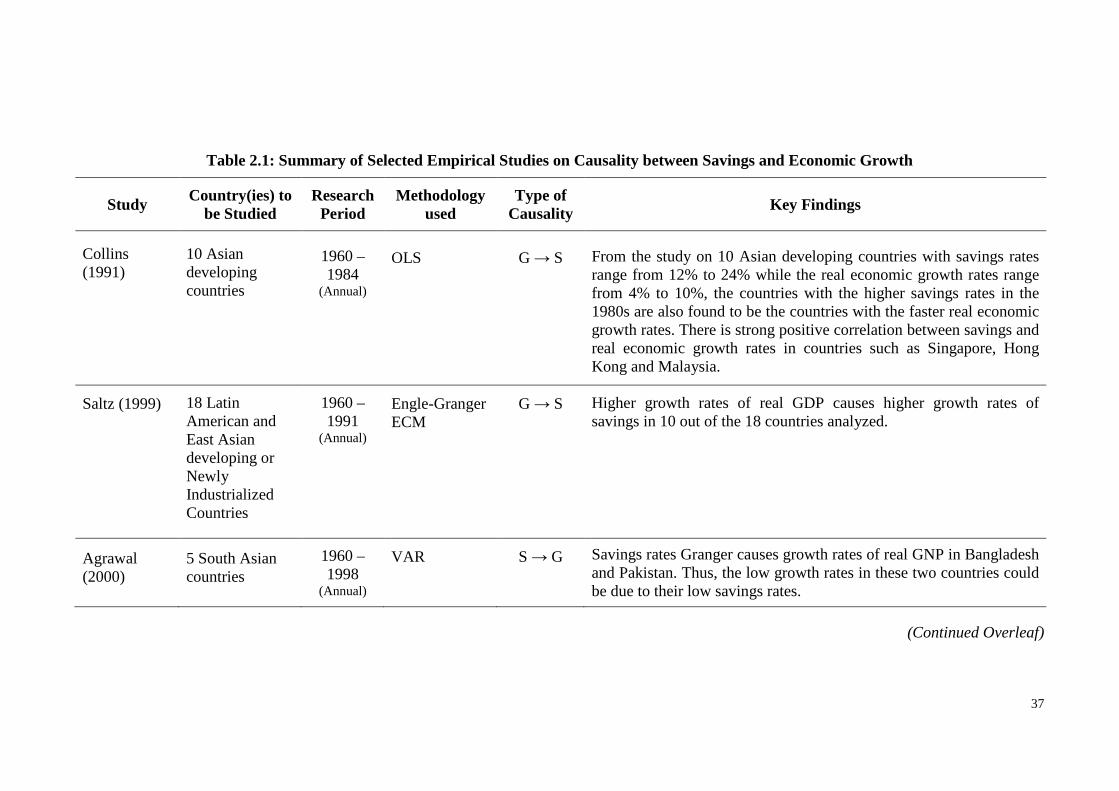
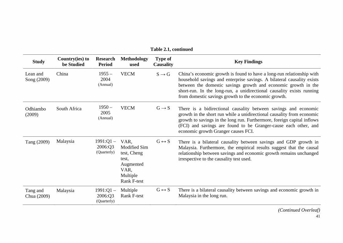
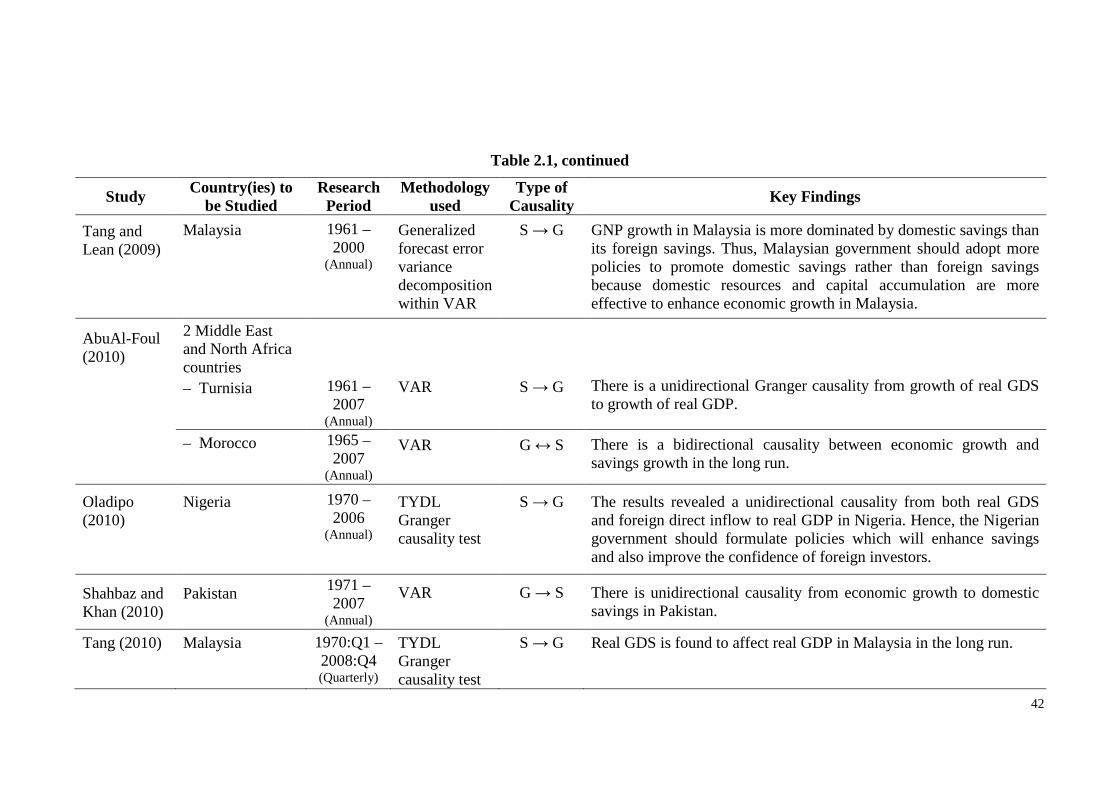
The key findings of selected empirical studies on causality between savings and

economic growth are summarized in Table 2.1. Most of the past empirical studies

showed that there is at least unidirectional causality between savings and growth. In

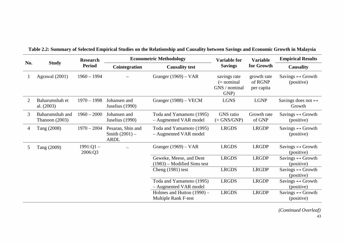
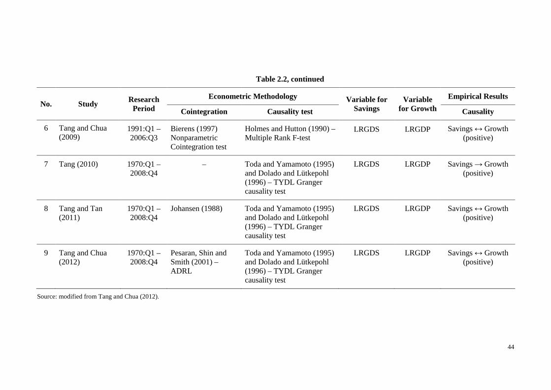
addition, the summary of selected empirical studies on the relationship and causality

between savings and economic growth in Malaysia is presented in Table 2.2. In

conclusion, a bidirectional causal relationship between savings and economic growth in

Malaysia was found by almost all researchers, irrespective of the research period and

econometric methodology used in their study.

2.4.4 No Causality

Although most of the past studies had found a direction of causality between savings

and economic growth in the country studied, there were few researchers did not get

evidence of causality between savings and growth in the country they studied. For

example, Baharumshah et al. (2003) had studied empirically the savings behavior in

five fast growth Asian economies, namely Singapore, South Korea, Malaysia, Thailand

and the Philippines using annual data of 1960–1997. They did not get any evidence of

causality between savings and economic growth in the short run for all the countries

examined, except for Singapore. It can be said that savings in the country may not an

important determinant of economic growth, and vice versa.

G ↑ ⇒ S ↑ ⇒ I ↑ ⇒ G ↑

37

Table 2.1: Summary of Selected Empirical Studies on Causality between Savings and Economic Growth

Study Country(ies) to

be Studied Research

Period Methodology

used Type of

Causality Key Findings

10 Asian developing countries

From the study on 10 Asian developing countries with savings rates range from 12% to 24% while the real economic growth rates range from 4% to 10%, the countries with the higher savings rates in the 1980s are also found to be the countries with the faster real economic growth rates. There is strong positive correlation between savings and real economic growth rates in countries such as Singapore, Hong Kong and Malaysia.

Collins (1991)

1960 – 1984

(Annual)

OLS

G → S

Saltz (1999)

18 Latin American and East Asian developing or Newly Industrialized Countries

1960 – 1991

(Annual)

Engle-Granger ECM

G → S

Higher growth rates of real GDP causes higher growth rates of savings in 10 out of the 18 countries analyzed.

Agrawal (2000)

5 South Asian countries

1960 – 1998

(Annual)

VAR

S → G

Savings rates Granger causes growth rates of real GNP in Bangladesh and Pakistan. Thus, the low growth rates in these two countries could be due to their low savings rates.

(Continued Overleaf)

38

Table 2.1, continued


be Studied Research Period

Methodology used

Type of Causality Key Findings

Deaton and Paxson (2000b)

Taiwan, Thailand

1976 – 1995

[Taiwan], 1976 – 1992

[Thailand] (Annual)

Method for estimating individual age-saving profiles using household data

G → S

By using individual age-savings profiles estimated from household data, increases in growth lead to large increases in savings rates in Taiwan, especially when there is low population growth rate. However, the empirical finding for Thailand was reverse whereby the relation is negative because of the increases in growth raise the wealth of the very young individuals who are dissavers. Thus, the aggregate savings rates is reduced.

Agrawal (2001)

7 Asian countries

1960 –1994

(Annual)

VAR, VECM

G → S

High savings rates in East Asian are mainly due to the high growth rates of income per capita and rapidly declining age dependency ratio. High real income per capita or high growth rate do Granger cause the savings rate to be high in six of the seven countries studied, except for Korea.

– Indonesia,

Malaysia, Taiwan

G ↔ S

There is evidence of simultaneous reverse causality from savings to growth for Indonesia, Malaysia and Taiwan. However, the causality from growth to savings is stronger than from savings to growth.

Anoruo and Ahmad (2001)

7 African countries

1960 – 1997

(Annual)

VECM

– Congo

S → G

Growth rate of domestic savings in Congo is found to Granger cause its growth rate of GDP.

– Ghana, Kenya, Nigeria,Zambia

G → S

Economic growth Granger causes growth rate of domestic savings in Ghana, Kenya, Nigeria, and Zambia.

– Cote d’Ivoire, South Africa

G ↔ S

There is a bidirectional causality between savings and growth. (Continued Overleaf)

39




Methodology used


Mavrotas and Kelly (2001)

India and Sri Lanka

1960 –1999

(Annual)

Toda and Yamamota Granger non-causality test

– India

G ↮ S

There is no causality between GDP growth and private savings in India.

– Sri Lanka

G ↔ S

There is a bidirectional causality between private savings and growth.

Baharumshah and Thanoon (2003)

Malaysia

1960 – 2000

(Annual)


G ↔ S

Bidirectional causality is detected between savings ratio and GNP growth in Malaysia. It can be concluded that economic growth plays an important role in explaining the high savings ratios in the past decades.

Alguacil et al. (2004)

Mexico

1970 – 2000

(Annual)


G ↔ S

There is a bidirectional causality between savings and economic growth provided that the influence of foreign capital inflows is taken into consideration in the study.


40




Methodology used


Mohan (2006)

25 countries with different income levels

1960 – 2000

(Annual)

VAR, VECM

G → S

The income class of a country is a crucial determinant of the direction of causality although there is no firm conclusion to be drawn for low-income countries. However, most of the low-middle income countries show that economic growth rate Granger causes growth rate of savings. Lastly, there is causality from economic growth to savings growth for all high-income countries except for Singapore and the United States.

Sajid and Sarfraz (2008)

Pakistan

1973:Q1 – 2003:Q4 (Quarterly)

VECM

G ↔ S

The findings suggest a bidirectional long-run relationship between savings and output level. However, there is a unidirectional causality from public savings to both GNP and GDP, and also from private savings to GNP in the long run.

Tang (2008)

Malaysia

1970 – 2004

(Annual)

Toda and Yamamota – Augmented VAR model

G ↔ S

There is a bilateral causal relationship between savings and income growth in Malaysia. This supports savings leads economic growth through the impact of capital formation. The savings is mobilized and financed into the productive activities.

Waithima (2008)

Kenya

1960 – 2005

(Annual)

VECM

G → S

GDP per capita Granger causes private savings in Kenya.


41




Methodology used


Lean and Song (2009)

China 1955 – 2004

(Annual)

VECM

S → G

China’s economic growth is found to have a long-run relationship with household savings and enterprise savings. A bilateral causality exists between the domestic savings growth and economic growth in the short-run. In the long-run, a unidirectional causality exists running from domestic savings growth to the economic growth.

Odhiambo (2009)

South Africa

1950 – 2005

(Annual)

VECM

G → S

There is a bidirectional causality between savings and economic growth in the short run while a unidirectional causality from economic growth to savings in the long run. Furthermore, foreign capital inflows (FCI) and savings are found to be Granger-cause each other, and economic growth Granger causes FCI.

Tang (2009)

Malaysia

1991:Q1 – 2006:Q3 (Quarterly)

VAR, Modified Sim test, Cheng test, Augmented VAR, Multiple Rank F-test

G ↔ S

There is a bilateral causality between savings and GDP growth in Malaysia. Furthermore, the empirical results suggest that the causal relationship between savings and economic growth remains unchanged irrespective to the causality test used.

Tang and Chua (2009)

Malaysia

1991:Q1 – 2006:Q3 (Quarterly)

Multiple Rank F-test

G ↔ S

There is a bilateral causality between savings and economic growth in Malaysia in the long run.


42




Methodology used


Tang and Lean (2009)

Malaysia

1961 – 2000

(Annual)

Generalized forecast error variance decomposition within VAR

S → G

GNP growth in Malaysia is more dominated by domestic savings than its foreign savings. Thus, Malaysian government should adopt more policies to promote domestic savings rather than foreign savings because domestic resources and capital accumulation are more effective to enhance economic growth in Malaysia.

AbuAl-Foul (2010)

2 Middle East and North Africa countries

– Turnisia 1961 –

2007 (Annual)

VAR S → G There is a unidirectional Granger causality from growth of real GDS to growth of real GDP.

– Morocco 1965 –

2007 (Annual)

VAR G ↔ S There is a bidirectional causality between economic growth and savings growth in the long run.

Oladipo (2010)

Nigeria

1970 – 2006

(Annual)

TYDL Granger causality test

S → G

The results revealed a unidirectional causality from both real GDS and foreign direct inflow to real GDP in Nigeria. Hence, the Nigerian government should formulate policies which will enhance savings and also improve the confidence of foreign investors.

Shahbaz and Khan (2010)

Pakistan

1971 – 2007

(Annual)

VAR

G → S

There is unidirectional causality from economic growth to domestic savings in Pakistan.

Tang (2010)

Malaysia

1970:Q1 – 2008:Q4 (Quarterly)

TYDL Granger causality test

S → G

Real GDS is found to affect real GDP in Malaysia in the long run.

43

Table 2.2: Summary of Selected Empirical Studies on the Relationship and Causality between Savings and Economic Growth in Malaysia

No. Study Research Period

Econometric Methodology Variable for Savings

Variable for Growth

Empirical Results

Cointegration Causality test Causality

1 Agrawal (2001) 1960 – 1994 – Granger (1969) – VAR savings rate growth rate Savings ↔ Growth

(= nominal GNS / nominal

GNP)

of RGNP per capita

(positive)

2

Baharumshah et al. (2003)

1970 – 1998

Johansen and Juselius (1990)

Granger (1988) – VECM

LGNS

LGNP

Savings does not ↔ Growth

3


1960 – 2000

Johansen and Juselius (1990)

Toda and Yamamoto (1995) – Augmented VAR model

GNS ratio (= GNS/GNP)

Growth rate of GNP

Savings ↔ Growth (positive)

4

Tang (2008)

1970 – 2004

Pesaran, Shin and Smith (2001) – ARDL


LRGDS

LRGDP


5 Tang (2009) 1991:Q1 – 2006:Q3

– Granger (1969) – VAR

LRGDS

LRGDP


Geweke, Meese, and Dent (1983) – Modified Sims test

LRGDS

LRGDP


Cheng (1981) test

LRGDS

LRGDP



LRGDS

LRGDP


Holmes and Hutton (1990) – Multiple Rank F-test

LRGDS

LRGDP



44


No. Study Research Period

Econometric Methodology Variable for Savings

Variable for Growth

Empirical Results

Cointegration Causality test Causality

6


1991:Q1 – 2006:Q3

Bierens (1997) Nonparametric Cointegration test

Holmes and Hutton (1990) – Multiple Rank F-test

LRGDS

LRGDP


7

Tang (2010)

1970:Q1 – 2008:Q4

–

Toda and Yamamoto (1995) and Dolado and Lütkepohl (1996) – TYDL Granger causality test

LRGDS

LRGDP

Savings → Growth (positive)

8

Tang and Tan (2011)

1970:Q1 – 2008:Q4

Johansen (1988)


LRGDS

LRGDP


9


1970:Q1 – 2008:Q4

Pesaran, Shin and Smith (2001) – ADRL


LRGDS

LRGDP


Source: modified from Tang and Chua (2012).

45

Sinha (1996) also did not get any causality between savings and growth in India using

annual data of 1950–1993 in his study. He found that there is no causality between the

growth rates of GDP and GDS, as well as between the growth rates of GDP and gross

domestic private savings (GDPS) in India. He commented that this could be due to the

savings not being channeled into productive investment in the country causing to the

insignificant relationship between savings and growth. These empirical results were

confirmed by Mavrotas and Kelly (2001) when they carried out a study on India.

The study on India was once again done by Sinha and Sinha (2007) when they carried

out a study to examine the relationship between per capita savings and per capita GDP

in India, which is one of the countries in the world with high savings rate, using data of

1950–2004. They distinguished the savings into three types, i.e. household savings,

corporate savings and public savings. By using Toda and Yamamota Granger causality

test which is seldom to be applied by researchers, they found that there is no evidence of

causality between per capita GDP and per capita corporate savings for India. The only

finding found from their study is that there is a bidirectional causality between per

capita household savings and per capita corporate savings.

2.5 Conclusion

This chapter has discussed the empirical works on the savings model and its derivatives

across many dimensions. The determinants of savings have been discussed. Empirical

works on causality between savings and economic growth has also been discussed. The

following chapter discusses the data sources, the variables and the econometric

techniques used in the empirical chapter.

46

CHAPTER 3 - ECONOMETRIC METHODOLOGY

3.1 Introduction

The previous chapter introduced the savings function by outlining its theoretical

background and empirical studies. In this chapter, Section 3.2 discusses the sample and

variables used while Section 3.3 explains the econometric techniques employed to test

the savings function in Malaysia.

3.2 Data Sources

The study examines the savings-led growth theory for Malaysia using multivariate

framework which consists of total five variables in estimating a savings equation. The

five variables are savings, income, age dependency ratio (ADR), interest rates (INT)

and Balance of Current Account (CAB) where CAB is as a proxy for foreign savings.

From the literature review, there are different measures used for savings and income (or

economic growth) in which the most common measures are either domestic data

statistics or national data statistics. For instance, Gross Domestic Savings (GDS) and

Gross Domestic Product (GDP) were used by Sinha (1996), Saltz (1999), Anoruo and

Ahmad (2001), Mohan (2006), Sajid and Sarfraz (2008), Tang (2008, 2009, 2010),

Tang and Chua (2009), AbuAl-Foul (2010), Oladipo (2010) and Tang and Tan (2011) to

estimate the savings equation in their studies.

On the other hand, Gross National Savings (GNS) and Gross National Product (GNP)

were used by Baharumshah et al. (2003) and Sajid and Sarfraz (2008). Despite domestic

savings is more common to be used, Agrawal (2001) stated that national savings is a

47

more appropriate measure of savings because it takes into consideration of the net factor

income from abroad, whereby the domestic savings does not. This net factor income

from abroad forms part of the savings in a country and is available to finance domestic

investment which will lead to higher growth of a country. In other words, national

savings reflects the total amount of resources available for domestic investment in a

country (Mason, 1988).

An annual data set consists of GDS, GDP, ADR, INT and CAB for the period from

1970 to 2010 is used in this study to estimate the GDS equation.4 Annual data is used

because of quarterly data is unavailable for certain variables such as ADR, INT and

CAB. The advantage of using annual data is it can avoid the seasonal bias problem

(Tang, 2008; Tang & Lean, 2008). Furthermore, Hakkio and Rush (1991) stated that

since cointegration is a long-run phenomenon, using longer span of data to give more

power to the cointegration test is better than merely increasing the data frequency but

shorter span of data [cited in Tang (2008)]. In conclusion, the span of data is more

important than the number of observations used in a study, as far as the ability of

cointegration is concerned [(Campbell & Perron, 1991; Hakkio & Rush, 1989; Hendry,

1987) cited in Thanoon and Baharumshah (2005)]. Arize and Shwiff (1998) argued that

data set containing fewer annual observations over a longer time period is preferable

than data set with more observations over a shorter time period for cointegration

analysis since increasing the sample size by time disaggregation may not likely to

reflect the long-run cointegrated relationship.

4 Instead of using GNS and GNP, GDS and GDP are used in this study because of domestic data statistics are commonly used in the previous studies for the causal relation between savings and economic growth in a country. In fact, Malaysian government adopts GDP in measuring the economic growth. Gross data rather than net data is used due to the availability of data and also because of the arbitrary nature of capital consumption allowances. However, Mason (1988) was in opinion that Net National Savings (NNS) is more ideal than GNS as NNS measures the total amount of resources from citizens of a country used for increasing the physical plant of that country whereas GNS may overestimate the actual increase in real wealth of a country.

48

In the past studies, real interest rates (RINT) is the variable which was more frequently

to be used for interest rates. However, from the unit root tests done in this study, RINT

was found to be stationary in level and cannot be used to proceed to cointegration

analysis. Thus, interest rates (INT) is used to substitute the RINT in this study.

The data of GDS, GDP, INT and CAB are extracted from Bank Negara Malaysia

publication, Monthly Statistical Bulletin while ADR is calculated using the data from

population statistics reports of Department of Statistics, Malaysia. The GDP deflator 5

(2000 = 100) is used to deflate GDS and GDP from nominal into real terms. To avoid

fluctuations in the data, all variables are transformed into natural logarithm (ln) terms

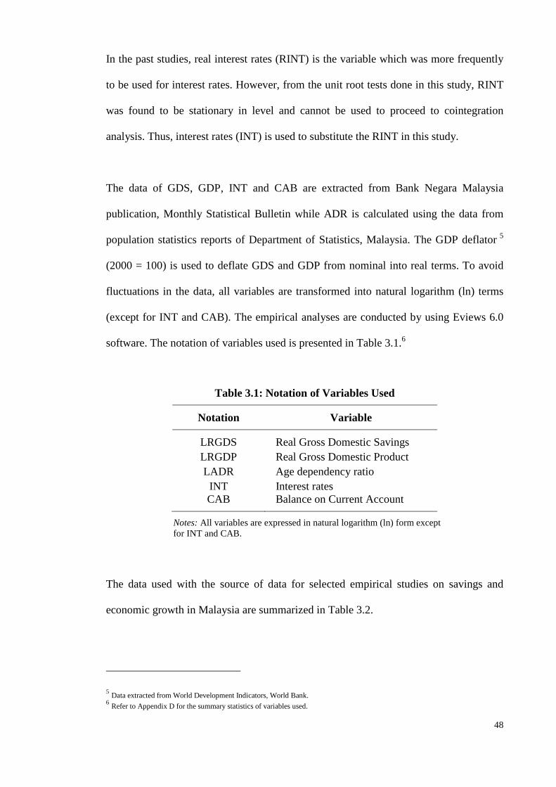
(except for INT and CAB). The empirical analyses are conducted by using Eviews 6.0

software. The notation of variables used is presented in Table 3.1.6

Table 3.1: Notation of Variables Used

Notation Variable

LRGDS Real Gross Domestic Savings LRGDP Real Gross Domestic Product LADR Age dependency ratio INT Interest rates CAB Balance on Current Account

Notes: All variables are expressed in natural logarithm (ln) form except for INT and CAB.

The data used with the source of data for selected empirical studies on savings and

economic growth in Malaysia are summarized in Table 3.2.

5 Data extracted from World Development Indicators, World Bank. 6 Refer to Appendix D for the summary statistics of variables used.

49

Table 3.2: Summary of Data Used in Selected Empirical Studies on Savings and Economic Growth in Malaysia

No. Study Data type Period Variables used Source of Data

1

Collins (1991)

Annual

1960 – 1985

ratio of GNS to GNP, real per capita income, real economic growth rate, young-age dependency ratio.

IMF; World Bank.

2

Hamid and Kanbur (1993)

Annual

1970 – 1990

real GNS, gross real disposable income, real interest rates, dependency ratio, inflation rate, Balance on Current Account (as a proxy for foreign savings).

BNM; World Bank.

3

Faruqee and Husain (1998)

Annual

1970 – 1992

ratio of private savings to private disposable income, working-age population ratio, growth in real private disposable income per capita, ratio of money plus quasi-money to private disposable income (as proxy to financial deepening), ratio of provident fund savings to private disposable income.

IMF; World Bank.

4

Agrawal (2001)

Annual

1960 – 1994

ratio of GNS to GNP, real GNP per capita, growth rate of GNP per capita, age dependency ratio, foreign savings (measured by Current Account Balance) as share of GNP, provident fund rate, real interest rates (on one year bank deposits).

World Bank; SEACEN Research & Training

Centre, Malaysia.

5


Annual

1960 – 2000

ratio of GNS to GNP, growth rate of GNP, interest rates, tax rate, exports rate, dependency ratio, Foreign Direct Investment.

ADB; World Bank; Key Indicators of Developing

Asian and Pacific Countries, 2001, Vol

XXXI, Oxford University Press, New York.


50


No. Study Data type Period Variables used Source of Data

6

Baharumshah et al. (2003)

Annual

1970 – 1998

GNS, GNP, interest rates, dependency ratio, current account.

IMF; BNM.

7

Thanoon and Baharumshah (2005)

Annual

1970 – 2000

ratio of GDS to GDP, age dependency ratio, rate of growth of GDP, per capita income, interest rates, ratio of Current Account Balance to GDP, export ratio to GDP, M2/GDP (as a proxy to degree of financial development.

Key Indicators of Developing Asian and Pacific Countries,

2002, Vol XXXI, Oxford University Press, New York.

8 Mohan (2006) Annual 1960 – 2001 GDS, GDP. World Bank

9

Tang (2008)

Annual

1970 – 2004

real GDS, real GDP, modified version of dependency ratio, real interest rates.

World Bank; IMF; BNM.

10 Tang (2009) Quarterly Jan 1991 – Sept 2006

real GDS, real GDP. IMF; BNM.

11 Tang and Chua (2009)

Quarterly Jan 1991 – Sept 2006

real GDS, real GDP. IMF; BNM.

12 Tang and Lean (2009)

Annual 1961 – 2000 real GNP, real disaggregate domestic & foreign savings. IMF; ADB; BNM; Malaysian Economic Report.

13

Tang (2010)

Quarterly

Jan 1970 – Dec 2008

real GDS, real GDP, real foreign capital inflow, real money supply M2 (as a proxy to financial development indicator).

World Bank; BNM.

14

Tang and Tan (2011)

Quarterly

Jan 1970 – Dec 2008

real GDS, real GDP, real interest rates, dependency ratio, current account (as a proxy for foreign savings).

World Bank; United Nations (UN), Statistical Yearbook for Asia and the Pacific.

15


Quarterly

Jan 1971 – Dec 2008

real GDS, real GDP, real interest rates, modified version of dependency ratio, real foreign savings.

World Bank; IMF; BNM.

51

3.3 Econometric Techniques

There are two main objectives for this empirical study. The first objective is to estimate

the savings function for Malaysia while the second objective is to examine the direction

of causality between savings and its determinants (see Section 1.7 for details). In

achieving these objectives, the econometric testing procedure involves four main steps.

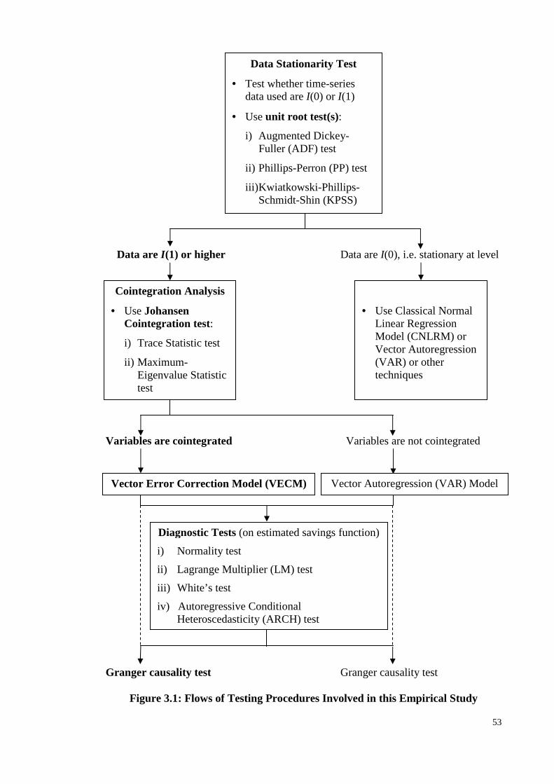
The first step is to check for the stationary properties of every variable using unit root

test(s). This step is crucial as it will examine the order of integration for the variables

and decide which appropriate procedure to be used in estimating the savings function.

The second step is to employ the cointegration analysis to examine whether there is

existence of long-run equilibrium relationship between savings and its determinants. If

cointegration is detected (meaning the variables are cointegrated and having a common

trend), it can be said that there is existence of Granger causality between variables at

least in one direction. However, the cointegration analysis did not manage to indicate

the direction of causality.

To investigate the direction of causality between savings and its determinants, the

following step is to obtain a long-run model using an unrestricted error correction model

(ECM). This model is namely Vector Error Correction Model (VECM) as it was

derived from the long-run cointegrating vector(s).

Various diagnostic tests on the estimated savings function are carried out to check on

the white noise property of residuals and to see whether the residuals are well-behaved.

52

Figure 3.1 depicts a flow chart as the summary for the flows of testing procedures

involved in this empirical study.

3.3.1 Stationary Tests – Unit Root Tests

In any empirical study or analysis using time series data, test of data stationarity (which

is a prerequisite for cointegration analysis) must be done first to check whether the time

series data used are individually stationary and also to avoid spurious regression. The

problem of spurious regression may occur when a time series variable is regressed on

another time series variable which does not have any logical relationship between them.

According to Granger and Newbold (1974), spurious or nonsense regression will exist

when there is presence of non-stationary variables [cited in Enders (2004)]. As a result,

spurious regression model tends to have a high R2, significant t-statistics, a high degree

of autocorrelation for its estimated residuals, and the assumption of the classical

regression model is violated (due to the variance found is heteroscedastic i.e. non-

constant and could be explosive). The results found from a spurious regression are

unreliable and without any economic meaning.

A stochastic process is said to be stationary if it fulfills the following requirements

simultaneously. The mean and variance are constant across time. Furthermore, the value

of the covariance between two time periods does not depend on the actual time at which

the covariance is computed, but depends only on the lag (or distance) between two time

periods (Gujarati, 2003).

53

Data are I(1) or higher Data are I(0), i.e. stationary at level

Variables are cointegrated Variables are not cointegrated

Granger causality test Granger causality test

Figure 3.1: Flows of Testing Procedures Involved in this Empirical Study

Data Stationarity Test

• Test whether time-series data used are I(0) or I(1)

• Use unit root test(s):

i) Augmented Dickey-Fuller (ADF) test

ii) Phillips-Perron (PP) test

iii) Kwiatkowski-Phillips-Schmidt-Shin (KPSS) test

Cointegration Analysis

• Use Johansen Cointegration test:

i) Trace Statistic test

ii) Maximum-Eigenvalue Statistic test

• Use Classical Normal Linear Regression Model (CNLRM) or Vector Autoregression (VAR) or other techniques

Vector Error Correction Model (VECM) Vector Autoregression (VAR) Model

Diagnostic Tests (on estimated savings function)

i) Normality test

ii) Lagrange Multiplier (LM) test

iii) White’s test

iv) Autoregressive Conditional Heteroscedasticity (ARCH) test

54

To determine the order of integration of all the variables used (or to test for the presence

of stochastic non-stationarity in the data used), three types of unit root tests, namely

Augmented Dickey-Fuller (ADF) test, Phillips-Perron (PP) test, and Kwiatkowski-

Phillips-Schmidt-Shin (KPSS) test will be employed. For these three unit root tests,

model with intercept and time trend will be chosen. The optimal lag length will be

decided by Akaike Info Criterion (AIC) for ADF test, while PP test and KPSS test will

be based on Newey-West Bandwidth with Barlett Kernel estimation method.

3.3.1.1 Augmented Dickey-Fuller (ADF) Test

Among the various unit root tests, ADF test is the most commonly used test. ADF test

was originated from the Dickey-Fuller (DF) test which can be employed if the error

terms (ut) are uncorrelated [i.e. independently and identically distributed (i.i.d.)].

However, DF test cannot be used if the error terms are correlated. In this case, the ADF

test should be used as this test is conducted by “augmenting” the equation of DF test by

adding the lagged difference terms of the dependent variable, so that the ut is serially

uncorrelated [(Dickey & Fuller, 1979, 1981) cited in Gujarati (2003)].

The regression (for a model with a drift and deterministic time trend) for ADF test is as

follows:

∆yt = µ + βt + δyt-1 +∑=

p

i 1

αi ∆yt-i + ut .................................. (3.1)

where ∆ is the difference operator, t is the time or trend variable. ut is a pure white noise

error term, �yt-1 = (yt-1 – yt-2), �yt-2 = (yt-2 – yt-3) and so on. The drift or intercept (refers

µ) and the deterministic time trend (refers βt) terms are retained if they are significantly

different from zero. The optimal lag length (p) will be determined by choosing the value

that minimizes the AIC.

55

The null hypothesis is that yt series is non-stationary (i.e. contains a unit root) which

implies that the δ in equation (3.1) equals zero whereas the alternative hypothesis states

that the series is stationary which implies δ is smaller than zero.

The test statistic used is the τ (tau) statistic computed using the following formula:

τ = ).(. δ

δ∧

∧

es .................................................... (3.2)

where s.e. is standard error. The test statistic is then compared with the critical values

tabulated by MacKinnon (1996). The null hypothesis of non-stationary is rejected if the

δ is negative and statistically significant (when the computed test-statistic value is

smaller than the critical value). Thus, there is evidence to conclude that yt series is a

stationary process. In contrast, if the null hypothesis is not rejected, this process is

repeated with the next higher order of differencing, until a rejection of null hypothesis is

found.

A variable or series without unit root is said to be stationary or integrated of order zero

[denoted by I(0)]. Thus, a series (for example, yt) which is stationary after being

differenced once is said to be integrated of order one [i.e. yt ~ I(1) and ∆yt ~ I(0)]. Most

of the time series data are found to be non-stationary in the level form but is stationary

in the first-difference form.

3.3.1.2 Phillips-Perron (PP) Test

The ADF test assumes and ensures that the error terms are uncorrelated in its regression.

However, the alternative unit root test, i.e. Phillips-Perron (1988) test can be used if the

56

residuals of a unit root process are weakly dependent or heterogeneous, since the PP test

allows for mildly correlated and heteroscedastic error terms (Enders, 2004).

The regression (for a model with a drift and deterministic time trend) for PP test is as

follows:

∆yt = µ + βt + δyt-1 + ut ........................................... (3.3)

where the only difference between the regression of ADF and PP tests is that PP test

does not consider the augmented term (i.e. the lagged difference terms of the dependent

variable).

The null hypothesis against alternative hypothesis, the critical values, and the procedure

used to reject a null hypothesis are the same as the ADF test.

A non-parametric correction to the t-test statistic is undertaken in the PP test to consider

for the possibility of the existence of serial correlation. Thus, the asymptotic distribution

of the test statistic will not be affected by the problem of serial correlation (Ang, 2009).

3.3.1.3 Kwiatowski-Phillips-Schmidt and Shin (KPSS) Test

For the ADF and PP tests, the null hypothesis is that a series is non-stationary (i.e. there

is existence of a unit root). Thus, rejection of the null hypothesis is necessary to support

stationarity of a series. However, according to Kwiatowski, Phillips, Schmidt and Shin

(1992), the tests designed on the basis of the null hypothesis that a series is non-

stationary (such as the ADF and PP tests) have low power to differentiate between unit

root and a near unit root stationary process and therefore, unable to reject the null

hypothesis. Thus, it is necessary to perform the KPSS test as well to confirm the order

of integration for all the variables used [cited in Ang (2009) and Tang (2009)].

57

The model with a drift and time trend for the KPSS test is based on a time series as

given in equation (3.4).

yt = µ + βt + ρyt-1 + ut ........................................... (3.4)

where µ is a drift or constant, βt is the deterministic time trend term, ρyt-1 refers to a

random walk process, and ut is an error term. Because of a random walk process can be

represented by the sum of all past errors, equation (3.4) can be written as follows:

yt = µ + βt + ϕ∑=

t

i 1

ut-i + εt ........................................ (3.5)

where ut is assumed to follow i.i.d. (0, 1), and εt is a stationary process.

As inverse to the ADF and PP tests, the null hypothesis of KPSS test states that the yt

series is trend stationary (i.e. stationary around a deterministic trend) which implies that

the ϕ in equation (3.5) equals zero while the alternative hypothesis states that the series

is not trend stationary which implies that ϕ does not equal to zero.

The test statistic used can be computed as follows:

LM = T -2 ∑=

T

t 1

2tS / σ2(p) ........................................... (3.6)

where T refers the number of observations, 2tS is the partial sum process of the residuals

from a regression of yt on an intercept and time, σ2(p) is a consistent estimate of the

error variance from the same regression, and p represents the lad truncation parameter

(Ang, 2009).

The LM-test statistic is then compared with the critical values provided by Kwiatkowski

et al. (1992) based on Monte Carlo simulation. The null hypothesis is rejected when the

58

LM-test statistic is larger than the critical value. In this case, there is evidence to say that

the yt series is a non-stationary time series.

3.3.2 Cointegration Analysis

Despite the regression of a non-stationary variable on another non-stationary variable

may produce the problem of spurious regression, according to Engle and Granger

(1987) who introduced the methodology of cointegration, a linear combination of two

non-stationary variables must be stationary if the error term (from the combination of

these two series) is stationary, i.e. ut ~ I(0). This is because of the underlying stochastic

trend in the two series will ‘cancel out’ one another when the cointegration takes place.

In this case, the two variables are said to be cointegrated and there will be existence of a

long-run equilibrium relationship among them. Granger (1986) stated that cointegration

test can be used to avoid spurious regression situations [cited in Gujarati (2003)].

Engle and Granger (1987) further highlighted that cointegration refer to a linear

combination, the variables which are cointegrated must be non-stationary variables with

the same order of integration, and there may be as many as (n – 1) linearly

independently cointegrating vectors for a vector yt which have n non-stationary

components (or variables). The number of cointegrating vectors is the cointegrating

rank of yt as well which tells us the number of linear relationship that exist in the model.

Engle and Granger (1987) mentioned that the existence of cointegrating relationship

between two variables also implies for the existence of a valid error-correction model

(ECM) between the two variables in which the data are generated according to a partial

adjustment or error-correction mechanism. After short-run deviations from the

equilibrium, the error term (which is known as equilibrium error) will ensure the system

59

to return to its long-run equilibrium. The linkage between concept of cointegration and

ECM is the essence of Granger Representation Theorem. In conclusion, besides short-

run dynamic relationship between the variables in a model, the error correction term

(ect) in the ECM incorporates the long-run information about the variables as well. The

ect tells us the speed for the model to return to its equilibrium following an exogenous

shock. A negative ect indicates a move back towards equilibrium, and vice versa.

All the non-stationary variables used must be first-differenced (in order to produce

stationary variables) because an ECM is derived based on I(0) variables only.

When the sample size of a study grows larger, or when there are more than two

variables used which may lead to multiple cointegrating vectors, Engle-Granger

methodology (which assumes that there is only one cointegrating vector) is not

appropriate to be used anymore. Methodology such as Johansen (1988) Cointegration

test can be employed as it is able to test for presence of multiple cointegrating vectors

by determining the cointegrating relationship among a set of integrated variables and

then incorporating then into an empirical model namely VECM.

3.3.2.1 Johansen Cointegration Test

The cointegration test which was developed by Johansen (1988) and then extended by

Johansen and Juselius (1990) will be used in this study to assess the existence of a long-

run relationship between savings and its determinants in Malaysia.

After examined the order of integration using unit root test(s), the next procedure is to

estimate a VAR model using the undifferenced data. As similar to the ADF test, a

multivariate model can also be generalized to allow for a higher-order autoregression

60

process (Enders, 2004). Assume that yt is a (n x 1) vector of I(1) variables, i.e. yt = (y1t ,

y2t , ........, ynt)’, and yt is non-stationary, i.e. yt ~ I(1), we can estimate the following

VAR(p) model for yt :

yt = A0 + A1yt-1 + A2yt-2 + …… + Apyt-p + ut .......................... (3.7)

where yt = (n x 1) vector of variables

A0 = (n x 1) matrix of intercept terms [i.e. (a01, a02, ........, a0n)’]

Ai = (n x n) matrices of coefficients (or parameters)

p = lag length

ut = an independently and identically distributed n-dimensional vector with zero

mean and variance matrix Ʃu

n = number of endogenous variables

Lag length (p) can be determined by using the multivariate generalizations of the AIC or

Schwartz Bayesian Criterion (SBC). Enders (2004, p. 358) stated that ‘most researchers

would begin with lag length of approximately T1/3’ where T refers the number of

observations used in a study.

Equation (3.7) can be re-written in the form of a VECM as follows: [See Enders (2004,

p. 352) for the mathematical manipulations]

∆yt = A0 + π yt-1 + ∑−

=

1

1

p

i

πi ∆yt-i + ut ................. (3.8)

Form of matrix: (n x 1) (n x 1) (n x n) (n x 1) (n x n) (n x 1) (n x 1)

where π = – ( I – ∑=

p

i 1

Ai) and πi = –∑+=

p

ij 1

Aj in which π = (n x n) matrix – ( I – Ai),

I = an (n x n) identity matrix, and πij denotes the element in row i and column j of π.

From equation (3.8), π refers to the rank of the matrix. The rank of π is equal to the

number of the independent cointegrating vectors (which is same number as the

61

cointegrating rank (r) of yt). The cointegrating rank will tell us whether the variables in

the model are cointegrated and also the number of long-run cointegrating relationship

which exist in the estimated model. The Granger Representation Theorem stated that the

rank (π) has a reduced rank where 0 < π < n. This is because if the rank (π) equals zero

(meaning no integration is found among the variables), the matrix will become null and

equation (3.8) will become ∆yt = A0 + ∑−

=

1

1

p

i

πi ∆yt-i + ut (which is actually a usual VAR

model in first differences). Thus, we have to use the approach of VAR instead of

VECM to estimate the regression.

In contrast, if π equals n (in other words, π has full rank), the model given by equation

(3.8) can be reduced to equation (3.7), showing that all variables are stationary and thus,

a VAR model in yt (levels) should be used. This is a trivial case of cointegration. In

intermediate case, if rank (π) equals one, there will be only one single cointergrating

vector and the expression πyt-1 in equation (3.8) is the ect of the model. In conclusion,

there will be multiple cointegrating vectors if the rank (π) is in between l and n, i.e.

1 < π < n.

In order to test other restrictions on the cointegrating vector, Johansen defines the two

matrices α and β, both of dimension (n x r) where r is the rank of π (Enders, 2004). The

properties of α and β are such that

π = α β’ ............................................. (3.9)

Form of matrix: (n x n) (n x r) (r x n)

in which α is the matrix of weights with which each cointegrating vector enters the n

equations of the VAR model while β is the matrix of cointegrating parameters. By

substituting equation (3.9) into equation (3.8), we get

62

∆yt = A0 + αβ’yt-1 + ∑−

=

1

1

p

i

πi ∆yt-i + ut ............................. (3.10)

where α = (n x r) matrix of the speed of adjustment parameters

β’ = (r x n) matrix of cointegrating vectors, in which r refers to the row, and n

refers to the column of the matrix

β’yt-1 = error correction term(s) which is (are) stationary

The vector α in the equation (3.10) measures how fast the deviations from equilibrium

move back into the system. A negative α indicates a move back towards equilibrium,

and vice versa. The larger the α, the faster for the convergence to take place towards the

long-run equilibrium when there are short-run deviations from its equilibrium (Ang,

2009). Besides, the β’ is actually the long-run coefficients in the VECM. The existence

of αβ’yt-1 leads to the main difference between a VAR model and VECM.

3.3.2.1.1 Trace Statistic Test

It is crucial to know how many cointegrating or long-term relationship (r) exist in a

model before we can estimate a VECM. Thus, Johansen proposes two likelihood ratio

statistic tests, namely the Trace Statistic test and the Maximum-Eigenvalue Statistic test

to test for the rank of the long-run information rank.

According to the Trace Statistic test, the null hypothesis (H0) which states that the

number of cointegrating relationship is less than or equal to r is tested against the

alternative hypothesis (Ha) which states that the number of cointegrating relationship is

greater than r. For example, H0: r = 0 is tested against Ha: r > 0; H0: r ≤ 1 against

Ha: r > 1; H0: r ≤ 2 against Ha: r > 2, and so on.

63

The test statistic used is as follows:

λtrace(r) = – T ∑+=

n

ri 1

ln (1 – ∧λ i ) ..................................... (3.11)

where T = the number of observations used in the study

∧λ i = the estimated values of the characteristic roots (also called eigenvalues)

obtained from the estimated π matrix [See Enders (2004, p. 386) for details]

The computed test statistic, λtrace is then compared with critical values tabulated by

Osterwald-Lenum (1992) using Monte Carlo approach. The null hypothesis will be

rejected if the test statistic is greater than the critical value. If so, this process is repeated

with the next higher number of cointergrating relationship (r) until there is no more

rejection of null hypothesis. At the end of the process, yt is said to be cointegrated with r

cointegrating relationship (and there will be r cointegrating vectors(s) for the VECM).

In this case, there will be (n – r) common stochastic trends for yt. In contrast, if H0: r = 0

is not rejected, there is evidence to say that there is no cointegrating relationship exists

in the model being tested.

3.3.2.1.2 Maximum-Eigenvalue Statistic Test

Maximum-Eigenvalue Statistic test can complement the Trace Statistic test in looking

for the number of cointergrating relationship (r) of a model, besides verifying the r

found using the Trace Statistic Test. In this statistic test, the null hypothesis (H0) which

states that the number of cointegrating relationship equals r is tested against the

alternative hypothesis (Ha) of r + 1. For example, H0: r = 0 is tested against Ha: r = 1;

H0: r = 1 against Ha: r = 2, and so on.

64

The test statistic is computed as follows:

λmax(r, r +1) = – T ln (1 – ∧λ r+1 ) .................................. (3.12)

where T = the number of observations used in the study

∧λ i = the estimated values of characteristic roots obtained from estimated π matrix

The computed test statistic, λmax is then compared with the critical values tabulated by

Osterwald-Lenum (1992) as well. The procedure used to reject a null hypothesis and the

implications of the result found are the same as the Trace Statistic test.

Maximum-Eigenvalue test has a specific or sharper alternative hypothesis, if compare

with the Trace Statistic test, An example used by Enders (2004) in his book had proven

that ‘Maximum-Eigenvalue test is usually preferred for trying to pin down the number

of cointegrating vectors’ (Ender, 2004, p. 354) meaning the Maximum-Eigenvalue test

will sometimes suggest for a smaller number of long-run relationship.

3.3.2.1.3 Vector Error Correction Model (VECM)

According to Engle and Granger (1987), a model with cointegrated variables must have

an error correction representation in which an ect is incorporated into the model. This

finding is then lead to the formation of VECM which incorporate the long-run

equilibrium as well as short-run dynamics in a model, so that the long-run information

is not lost during the differencing process.

Once the number of cointegrating relationship (r) is determined by using the Trace

and/or Maximum-Eigenvalue Statistic test(s), a VECM [refer to equation (3.10)] can be

estimated based on Ordinary Least Squares (OLS) method. Since the ect (i.e. β’yt-1) and

65

all values of ∆yt-i from equation (3.10) are stationary, we can inference on any variables

(except those appearing within the cointegrating vectors) using the usual test statistics.

In this study, to estimate a VECM for domestic savings in Malaysia, five variables are

used (n = 5), namely LRGDS, LRGDP, LADR, INT and CAB. Assuming there are two

cointegrating relationships (r = 2) exist in the domestic savings model, and two lags (p

= 2) are used in the VECM. Thus, yt = (y1t , y2t , y3t , y4t , y5t)’ becomes

yt = (LRGDSt , LRGDPt , LADRt , INTt , CABt)’ 7....................... (3.13)

In the Johansen test, all the variables used are treated as endogenous variable in a VAR

framework. From the VAR(2) model for yt, the respective VECM for domestic savings

and GDP can be written as follows:

∆LRGDSt = a0 + α11(β11LRGDSt-1 + β12LRGDPt-1 + β13LADRt-1 + β14INTt-1 + β15CABt-1) +

α12(β21LRGDSt-1 + β22LRGDPt-1 + β23LADRt-1 + β24INTt-1 + β25CABt-1) +

∑=

2

1i

a1i ∆LRGDSt-i + ∑=

2

1i

a2i ∆LRGDPt-i + ∑=

2

1i

a3i ∆LADRt-i + ∑=

2

1i

a4i ∆INTt-i

+ ∑=

2

1i

a5i ∆CABt-i + u1t ......................................................................... (3.14)

∆LRGDPt = b0 + α21(β11LRGDSt-1 + β12LRGDPt-1 + β13LADRt-1 + β14INTt-1 + β15CABt-1) +

α22(β21LRGDSt-1 + β22LRGDPt-1 + β23LADRt-1 + β24INTt-1 + β25CABt-1) +

∑=

2

1i

b1i ∆LRGDSt-i + ∑=

2

1i

b2i ∆LRGDPt-i + ∑=

2

1i

b3i ∆LADRt-i + ∑=

2

1i

b4i ∆INTt-i

+ ∑=

2

1i

b5i ∆CABt-i + u2t ......................................................................... (3.15)

7 The number of variables to be included in the yt vector is subject to the empirical results from unit root test(s). The yt vector will include only I(1) variables in estimating the VECM.

66

where the two error correction terms (ect) are:

ect1t-1 = β11LRGDSt-1 + β12LRGDPt-1 + β13LADRt-1 + β14INTt-1 + β15CABt-1 .............. (3.16)

ect2t-1 = β21LRGDSt-1 + β22LRGDPt-1 + β23LADRt-1 + β24INTt-1 + β25CABt-1 .............. (3.17)

The long-run relationship of a particular variable can be obtained by normalizing on that

particular variable by making its coefficient equal to one. By setting ect1t = 0 and ect2t =

0, we get:

β11LRGDSt + β12LRGDPt + β13LADRt + β14INTt + β15CABt = 0 or,

LRGDSt = – (β12 /β11)LRGDPt – (β13 /β11)LADRt – (β14 /β11)INTt – (β15 /β11)CABt ....(3.18)

β21LRGDSt + β22LRGDPt + β23LADRt + β24INTt + β25CABt = 0 or,

LRGDPt = – (β21 /β22)LRGDSt – (β23 /β22)LADRt – (β24 /β22)INTt – (β25 /β22)CABt ....(3.19)

Equation (3.18) shows the long-run domestic savings model when we normalize on

LRGDSt by setting the ect1t equal to zero. Similarly, we obtain the long-run GDP model

as shown by equation (3.19) when we normalize on LRGDPt by setting the ect2t equal to

zero.

From the equation (3.14), α11 and α12 are speed of adjustment coefficients which

measure how fast the ∆LRGDSt will adjust to return to its long-run equilibrium.

3.3.3 Diagnostic Tests

The residuals in the estimated savings equation of the study are assumed to be

independently and identically distributed (i.i.d.) and well-behaved. To verify this

assumption and to check on the reliability of estimation and results found, various

diagnostic tests should be carried out (see Section 3.3.3.1 to 3.3.3.4 for the details).

67

3.3.3.1 Normality Test

Normality test can be used to check for the normality of residuals of an estimated

regression. Among several tests of normality, the more common methods of testing for

normality of residuals are histogram of residuals, and Jarque-Bera (JB) test. A

histogram of residuals is a simple graphic device used to show the shape of probability

density function (PDF) of the estimated residuals from a regression. From a histogram,

we can see whether the residuals are symmetrically distributed (Gujarati, 2003).

In this study, Jarque-Bera (JB) test of normality will be used. It is an asymptotic or

larger-sample test based on the OLS residuals. The JB test will compute the skewness

and kurtosis measures of the residuals first and then computes the test statistic using the

formula as follows:

....................................... (3.20)

where n = sample size, S = skewness coefficient, and K = kurtosis coefficient. The

value of the JB test statistic is expected to be zero because for a normally distributed

variable, S should be equal to zero, and K should be three (Gujarati, 2003).

The null hypothesis of the JB test states that the residuals are normally distributed. We

will reject the null hypothesis if the value of JB test statistic is very different from zero,

and its computed p-value is sufficiently low. In contrast, if the value of test statistic is

close to zero, and a reasonably high p-value is found, we do not reject the null

hypothesis that the residuals are normally distributed.

68

3.3.3.2 Lagrange Multiplier (LM) Test

Breusch-Godfrey (BG) Lagrange Multiplier (LM) test is used to test the residuals of the

estimated savings equation for serial correlation. The advantage of this type of LM test

is that this test of autocorrelation allows for higher-order autoregressive schemes (i.e.

AR(1), AR(2), and so on), simple or higher moving averages of white noise error terms

(i.e. εt in ut = ρut-1 + εt where –1 < ρ < 1), and also non-stochastic regressors, such as the

lagged values of the dependent variables (Gujarati, 2003).

The test statistic used is (n – p)R2 where n is the sample size, p is the order of

autoregressive scheme, and R2 is R-square value obtained from the auxiliary regression

(of estimated residuals) follows the chi-square distribution with p degree of freedom.

The null hypothesis which states that there is no serial correlation of any order is tested.

If the computed test statistic value exceeds the critical chi-square value, in other words,

the p-value is statistically significant at a chosen level of significance, we will reject the

null hypothesis, and vice versa.

3.3.3.3 Heteroscedasticity Test

Heteroscedasticity refers a systematic pattern in the errors of a regression model where

the variances of the error are not constant. As the consequences of heteroscedasticity,

the OLS estimators are no longer best linear unbiased estimator (BLUE) and will be

inefficient. Thus, the forecasts will also be inefficient (Gujarati, 2003).

69

White’s general heteroscedasticity test will be used to detect the problem of

heteroscedasticity since this test is easy to be implemented and it does not rely on the

normality assumption.

The test statistic used is nR2 where n is the sample size, and R2 is the R-square value

obtained from the auxiliary regression asymptotically follows the chi-square distribution

with degree of freedom equals the number of regressors (excluding the constant term) in

the auxiliary regression.

The null hypothesis which states that there is no heteroscedasticity is rejected if the

computed test statistic value exceeds the critical chi-square value, or the p-value is

statistically significant at a chosen level of significance. In such a case, we have

evidence of heteroscedasticity.

3.3.3.4 Autoregressive Conditional Heteroscedasticity (ARCH) Test

For modeling conditional mean of a random variable, the variance of the process is

assumed to be constant. However, there are many time series data in which the volatility

is not constant overtime. Thus, ARCH-type models are useful to model volatility, to

obtain more efficient estimators by handling heteroscedasticity in errors properly, and to

obtain more accurate confidence intervals for forecast purpose.

Autoregressive Conditional Heteroscedasticity (ARCH) test developed by Engle is a

specification of heteroscedasticity where the variance of ut at period t depends on the

squared error term of the past periods. The null hypothesis, alternative hypothesis and

the formula used to compute the test statistic value in the ARCH test are the same as the

White’s heteroscedasticity test (in Section 3.3.3.3).

70

The null hypothesis of there is no autoregressive conditional heteroscedasticity is

rejected if the computed test statistic value exceeds the critical chi-square value, or the

p-value is statistically significance. Rejection of H0 is indicative of presence of ARCH.

Thus, the ARCH(q) model is suitable for modeling the conditional variance, where q

refers the order of first partial autocorrelation coefficient which is significant, found

from the Correlogram of Residuals Squared in Eviews.

3.3.4 Granger Causality Test

According to Granger (1969), an explanatory variable (X) is said to Granger cause a

dependent variable (Y) if and only if the past values of X can be used to explain Y more

accurately than just use the past values of Y (Abu, 2010). To investigate the causal

relationship between domestic savings and economic growth in Malaysia, Granger

(1988) Causality test is employed on the estimated VECM found for GDS [i.e. equation

(3.14)] and GDP [i.e. equation (3.15)] respectively. The causality from economic

growth to savings can occur in two ways, either through the impact of lagged changes in

economic growth, or through the lagged ect term(s) in the VECM of savings.8

The null hypothesis (H0) which states that an explanatory variable (X) does not Ganger

cause the dependent variable (Y) is tested against the alternative hypothesis (Ha) of the X

does Granger cause the Y. As an example, we use VECM of GDS, i.e. equation (3.14) to

test whether GDP Granger causes GDS in Malaysia. The H0: a21 = a22 = α11 = α12 = 0 is

tested against Ha: at least one of the restrictions is not true. From H0, although all the

coefficients of the lagged differences of the explanatory variable and the coefficient of

lagged ect term(s) have to be equals zero, VECM can reject H0 and allows for existence

8 In contrast, savings Granger causes economic growth can occur in two ways, either through the impact of lagged changes in savings, or through the lagged ect term(s) in the VECM of economic growth.

71

of causality even if the coefficients stated in H0 are not jointly significant. Another

advantage of Granger causality test is that the cause of causality can be identified either

due to short-run dynamics or disequilibrium adjustment (Agrawal, 2001).

From the unrestricted model, i.e. equation (3.14), the restricted model is given as:

∆LRGDSt = a0 + ∑=

2

1i

a1i ∆LRGDSt-i + ∑=

2

1i

a3i ∆LADRt-i + ∑=

2

1i

a4i ∆INTt-i + ∑=

2

1i

a5i ∆CABt-i

+ u1t .................................................................................................... (3.21)

By using Wald test, the F-test statistic can be computed as follows:

F = ( RSSR – RSSU ) / z RSSU / (n – mp – 1 – r) ................................... (3.22)

where RSS is residual sum of squares, R is restricted model, U is unrestricted model, z is

the number of restrictions under H0, n is number of observations used in the study, m is

number of variables used, p is number of lags, and r is number of ect. The H0 is rejected

if the F-test statistic exceeds the critical value, Fα; z, n-mp-1-r at α level of significance.

Thus, there is evidence to say that GDP Granger causes GDS.

By the way, in equation (3.14), the H0 that GDP does not Ganger cause GDS is rejected

if any of a2i or α11 or α12 is statistically and significantly different from zero but neither

the b1i or α21 or α22 from equation (3.15) is statistically significant. Similarly, in

equation (3.15), the H0 that GDS does not Ganger cause GDP is rejected on the

condition that any of b1i or α21 or α22 is statistically and significantly different from zero

but neither the a2i or α11 or α12 from equation (3.14) is statistically significant. Table 3.3

summarizes the possible causal relationships which can be derived between domestic

savings (S) and economic growth (G), based on equations (3.14) and (3.15).

72

Table 3.3: Four Types of Causality between Savings and Economic Growth _________________________________________________________________________________________________ __________________________________________

Types of Causality Any One of the Conditions ___________________________________________________________________________________________________________________________________________________________________________________________________________________________________________________________________________________________

Unidirectional causality from growth to savings: Gt → St a2i ≠ 0; α11 ≠ 0; α12 ≠ 0.

Unidirectional causality from savings to growth: St → Gt b1i ≠ 0; α21 ≠ 0; α22 ≠ 0.

Bilateral causality: St ↔ Gt a2i ≠ 0; α11 ≠ 0; α12 ≠ 0; b1i ≠ 0; α21 ≠ 0; α22 ≠ 0.

No causality: St ↮ Gt a2i = 0; α11 = 0; α12 = 0; b1i = 0; α21 = 0; α22 = 0.

_____________________________________________________________________________________________________________________________________________

3.4 Conclusion

This chapter explains the data sources and methodology used. Firstly, three unit root

tests, namely ADF, PP and KPSS tests are used to check for the stationarity of variables

used. Secondly, Johansen methodology which considers only the stationary variables at

the same order of integration is used to examine the existence of long-run relationship

between savings and its determinants. The Trace and Maximum-Eigenvalue statistic

tests will indicate the number of cointegrating relationship(s) among the variables in the

savings function. A VECM is estimated to derive the long-run and short-run savings

functions in Malaysia. Next, various diagnostic tests are employed to verify the

reliability of estimation and results found. Lastly, Granger causality test on the

estimated VECM is applied to investigate the causal relationship between savings and

its determinants.

73

CHAPTER 4 - EMPIRICAL RESULTS AND ANALYSES

4.1 Introduction

In the previous chapter, the data sources and econometric methodology used have been

discussed. This chapter reports and interprets the results obtained from the whole

econometric testing procedures involved. To avoid spurious regression, the results of

unit root tests in Section 4.2 are very crucial to determine which variables to be used for

the Johansen cointegration analysis. After decided for the lag length to be used, the

results of Trace and Maximum-Eigenvalue Statistic tests which examine the number of

long-run cointegrating relationship exists between the variables used are explained in

Section 4.3. Following this, an error correction model (ECM) will be formed for

domestic savings in Malaysia. Section 4.4 presents the estimated long-run domestic

savings model in Malaysia, together with its short-run dynamic model and the

diagnostic test results. Lastly, the results for Granger causality between savings and its

determinants in Malaysia are highlighted in Section 4.5. Section 4.6 concludes the

chapter.

4.2 Unit Root Test Results

To assess the order of integration for all the variables used, three unit root tests, namely

ADF test, PP test, and KPSS test are employed in this study. The ADF and PP tests are

used to test for the null hypothesis of a unit root against the alternative of stationarity. In

contrast, the KPSS test is used to test the null hypothesis of stationarity against the

alternative of a unit root. For all these three unit root tests, the model with a drift and

deterministic trend is chosen to test all the variables.

74

For a model with intercept and a trend with zero lag length, for both ADF and PP tests,

the critical values, in level, are –4.2050, –3.5267 and –3.1946 at the 1%, 5% and 10%

levels of significance, respectively while the critical values, in first difference, are

–4.2119, –3.5298 and –3.1964 at the 1%, 5% and 10% levels of significance,

respectively. In contrast, for the KPSS test, the critical values, for both in level and

first difference, are 0.2160, 0.1460 and 0.1190 at the 1%, 5% and 10% levels of

significance, respectively.

The results of the unit root tests are presented in Table 4.1.9 In the level data, since the

test statistics of the ADF and PP tests are higher than the critical values, the null

hypothesis that the respective series contains a unit root cannot be rejected. However,

there is no evidence to support the existence of a unit root in first difference of all the

variables tested. Thus, the null hypothesis of a unit root in first difference is rejected at

the 1% level of significance for all the variables (except for ADR), and at the 5% level

of significance for ADR. Besides, the results of the KPSS test indicate that the null

hypothesis that the respective series is a stationary process in the level is rejected, at

either 5% or 10% level of significance, but is not rejected in the first difference, for all

variables tested.

Figure 4.1 shows the annual time series plots for the five variables used in this study.

All the variables suggest a linear trend in their series (except for INT and CAB which

are unclear for their linear trend). The variables are said to be not stationary in level due

to their non-constant mean. However, from the plots of the first difference for the

variables, they show stationarity due to the constant mean.

9 The results based on a model with a drift but no deterministic trend are not shown in this paper due to the similar results found from the use of a model with a drift and a deterministic trend in this study.

75

Table 4.1: Results of Unit Root Tests

Variable

ADF PP KPSS

Level First Difference

Level First Difference

Level First Difference Conclusion

LRGDSt –2.6234 –8.1652*** –2.3607 –9.3745*** 0.1733** 0.0210 I(1)

LRGDPt –1.9381 –6.6809*** –1.7972 –6.7814*** 0.1693** 0.0475 I(1) LADRt –1.5223 –4.1254** –1.1718 –4.1254** 0.1210* 0.0951 I(1) INTt –1.6377 –4.7959*** –2.4933 –8.7715*** 0.1412* 0.0805 I(1) CABt –1.5706 –5.0887*** –1.6514 –4.8364*** 0.1842** 0.0787 I(1)

Notes: ***, ** and * denote rejection of the corresponding null hypothesis at the 1%, 5% and 10% levels of significance, respectively. The ADF test is conducted with the optimal lag length chosen using AIC while the PP test and KPSS test are conducted with the optimal bandwidth chosen using Newey-West bandwidth with Barlett kernel estimation method respectively. The critical values for ADF and PP tests are obtained from MacKinnon (1996) while the asymptotic critical values for KPSS test are obtained from Kwiatkowski et al. (1992). Both of the ADF and PP tests examine the null hypothesis of a unit root against the stationarity and the KPSS test examines the null hypothesis of stationarity against the alternative of a unit root.

76

Figure 4.1: Time Series Properties

Figure 4.1a: LRGDS Figure 4.1b: Change in LRGDS (∆LRGDS)

9.0

9.5

10.0

10.5

11.0

11.5

12.0

12.5

1970 1975 1980 1985 1990 1995 2000 2005 2010

-.3

-.2

-.1

.0

.1

.2

.3

.4

.5

.6

1975 1980 1985 1990 1995 2000 2005 2010

Figure 4.1c: LRGDP Figure 4.1d: Change in LRGDP (∆LRGDP)

10.5

11.0

11.5

12.0

12.5

13.0

13.5

1970 1975 1980 1985 1990 1995 2000 2005 2010

-.10

-.05

.00

.05

.10

.15

.20

.25

1975 1980 1985 1990 1995 2000 2005 2010

Figure 4.1e: LADR Figure 4.1f: Change in LADR (∆LADR)

3.8

3.9

4.0

4.1

4.2

4.3

4.4

4.5

4.6

1970 1975 1980 1985 1990 1995 2000 2005 2010

-.030

-.025

-.020

-.015

-.010

-.005

.000

1975 1980 1985 1990 1995 2000 2005 2010

Figure 4.1g: INT Figure 4.1h: Change in INT (∆INT)

2

3

4

5

6

7

8

9

10

11

1970 1975 1980 1985 1990 1995 2000 2005 2010

-4

-3

-2

-1

0

1

2

3

1975 1980 1985 1990 1995 2000 2005 2010

77

Figure 4.1i: CAB Figure 4.1j: Change in CAB (∆CAB)

-40,000

0

40,000

80,000

120,000

160,000

1970 1975 1980 1985 1990 1995 2000 2005 2010

-30,000

-20,000

-10,000

0

10,000

20,000

30,000

40,000

50,000

1975 1980 1985 1990 1995 2000 2005 2010

In conclusion, all the five variables used are not stationary in the level form of the

variable, but they are stationary after taking the first difference. They are said to be

integrated of order one I(1) process. This result is consistent with the findings of Nelson

and Plosser (1982) who stated that most of the macroeconomic series which are non-

stationary in level will become stationary after their first differencing. Since all these

seven series are individually integrated of order one (and furthermore, at the same order

of integration), it is necessary to proceed to the next step, i.e. cointegration analysis to

test whether the variables are cointegrated in the long run.

4.3 Cointegration Test Results

The cointegration test which was developed by Johansen (1988) and then extended by

Johansen and Juselius (1990) was used in this study to examine the existence of long-

run cointegrating relationship(s) between savings and its determinants in Malaysia.

The first step in the cointegrating test is to determine the lag length for the savings

model. For a study uses annual data and the variables become stationary after their first

differencing, Sinha (1996) was in opinion that lag length of one can be used. He also

claimed that the number of lags used by applied researchers is up to two if their studies

78

use annual data. Furthermore, Mohan (2006) highlighted that the optimal lag length

should be smaller than three for a study uses annual data because a larger lag length in a

small sample will waste the degree of freedom. Besides, Enders (2004) mentioned that

lag length up to four can be used if the sample size is small and quarterly data set is

used. Thus, a lag of one is chosen for this study since the sample size is small and

annual data set is used. After decided for the lag length, it is then followed by the Trace

and Maximum-Eigenvalue Statistic tests to examine whether the variables used are

cointegrated.

The results of cointegration test produced by the Trace and Maximum-Eigenvalue

Statistic tests are summarized in Table 4.2.

Table 4.2: Results of Johansen Cointegration Test

Variables: LRGDSt , LRGDPt , LADRt , INTt , CABt

Hypothesis Trace Statistic Test

H0 Ha Trace Statistic 5% Critical Value p-value

r = 0 r > 0 83.94423*** 69.81889 0.0025 r ≤ 1 r > 1 49.70706** 47.85613 0.0331 r ≤ 2 r > 2 19.15351 29.79707 0.4819 r ≤ 3 r > 3 8.11809 15.49471 0.4529 r ≤ 4 r > 4 0.90179 3.84147 0.3423

Hypothesis Maximum-Eigenvalue Statistic Test

H0 Ha Maximum-Eigenvalue Statistic 5% Critical Value p-value

r = 0 r = 1 34.23717** 33.87687 0.0453 r = 1 r = 2 30.55355** 27.58434 0.0202 r = 2 r = 3 11.03542 21.13162 0.6438 r = 3 r = 4 7.21631 14.26460 0.4639 r = 4 r = 5 0.90179 3.84147 0.3423

Notes: r denotes the number of cointegrating vectors. ***, ** and * denote rejection of the corresponding null hypothesis at the 1%, 5% and 10% levels of significance, respectively. The p-values are obtained from MacKinnon, Haug & Michellis (1999).

79

For the first round, if the computed values of the Trace statistic and Maximum-

Eigenvalue statistic are less than their corresponding critical values at the 5% level of

significance, then the null hypothesis of no cointegration (r = 0) cannot be rejected.

However, since the statistic values are greater than their critical values and show

significant results, we then proceed to the next higher cointegrating rank. This process is

continued until the null hypothesis cannot be rejected.

In the first round, the Trace and Maximum-Eigenvalue statistic values reveal that the

null hypothesis of no cointegrating relation (r = 0) can be rejected at the 1% and 5%

levels of significance by the Trace and Maximum-Eigenvalue Statistic tests,

respectively. It is possible to accept the alternative of one or more cointegrating

relations. In the second round, the null hypothesis of one cointegrating relation is

rejected at the 5% level of significance by both of the tests. However, the two tests fail

to reject the null hypothesis of two cointegrating relations in the next round. Thus, at the

5% level of significance, both of the Trace and Maximum-Eigenvalue Statistic tests

confirm that there are two cointegrating relations (and vectors) exist among the

domestic savings, GDP, dependency ratio, interest rates and foreign savings in

Malaysia.

In conclusion, the variables used in this study are cointegrated. There is existence of

two cointegrating relations (and vectors) in the five-dimentional vector [LRGDS,

LRGDP, LADR, INT, CAB] of I(1) variables. The long-run relationships found between

domestic savings and its explanatory variables indicate that there must be causality in at

least one direction among the variables. However, the direction of causality can only be

detected through the Vector Error Correction Model (VECM) which is derived from the

two cointegrating vectors in this study.

80

4.4 Long-run Equilibrium Estimates of Savings Equation

As the variables used are cointegrated, the long-run equilibrium domestic savings

equation can be estimated by using the VECM approach. Table 4.3 depicts the long-run

relationships exist in the domestic savings equation, by normalizing the cointegrating

vectors on savings and interest rates, respectively. The estimated long-run domestic

savings function in Malaysia, obtained from the first cointegrating vector of the

domestic savings equation is given by equation (4.1) whereas the second cointegrating

vector of the domestic savings equation is shown by equation (4.2).

LRGDSt = 1.0073LRGDPt*** – 1.5850LADRt** – 0.000003CABt*** + 5.6416 .....(4.1)

INTt = –15.0401LRGDPt* – 70.9504LADRt* – 0.00016CABt*** + 491.0515 ........(4.2)

Table 4.3: Normalized Cointegrating Vectors

Variable First Cointegrating Vector Second Cointegrating Vector

LRGDSt 1.0000 0.0000

LRGDPt 1.0073*** –15.0401* (0.1162) (7.5733)

LADRt –1.5850** –70.9504* (0.6415) (41.8036)

INTt 0.0000 1.0000

CABt –0.000003*** –0.00016*** (0.0000006) (0.00004)

constant 5.6416 491.0515

Notes: The estimated coefficients were obtained by normalizing the savings and interest rates variables, respectively from the domestic savings equation. ***, ** and * denote significance at the 1%, 5% and 10% levels of significance, respectively. Figures in parentheses are the standard errors.

Since all the variables used are in natural logarithm (ln) term (except for interest rates

and foreign savings), the estimated coefficients in equation (4.1) can be interpreted as

long-run elasticities of domestic savings with respect to the particular variable (except

for interest rates and foreign savings).

81

From the long-run domestic savings equation, the results show that savings in Malaysia

is positively related to income in the long run, with an estimated long-run elasticity of

savings with respect to GDP equals 1.0073 and it is statistically significant at the 1%

significance level. Empirically, a one percent increase in GDP leads to 1.0073 percent

increase in domestic savings. The finding of a positive and significant role of income

variable on savings in Malaysia is consistent with the results from past studies, such as

Baharumshah and Thanoon (2003), Baharumshah et al. (2003), Thanoon and

Baharumshah (2005), Tang (2008, 2009), Agrawal et al. (2009), and Tang and Chua

(2009, 2012). Besides, the empirical result found supports the Life Cycle Hypothesis

(LCH) as was discussed in Section 2.4.2 which states that higher economic growth or

income growth raises the savings in a country. In reality, high economic performance of

Malaysia is one of the main determinants of high savings rates in the country.

On the other hand, the coefficient of age dependency ratio (ADR) is found to be

negative and statistically significant at the 5% significance level in the savings equation,

with an estimated long-run elasticity of savings with respect to dependency ratio equals

–1.5850. With the highest magnitude (if compare with other variables) in the savings

equation, age dependency ratio (i.e. demographic or age structure of the population)

seems to be the most important determinant of savings in Malaysia in the long run. This

result implies that a one percent decline in dependency ratio in the long run increases

domestic savings in Malaysia by 1.5850 percent. The importance of demographic

variable supports the LCH (discussed in Section 2.3.2) proposed by Modigliani (1970)

and is consistent with the previous studies by Leff (1969), Edwards (1996), Loayza et

al. (2000), Agrawal (2001), Baharumshah and Thanoon (2003), Thanoon and

Baharumshah (2005), Agrawal et al. (2009), Tang and Tan (2011), and Tang and Chua

(2012).

82

Similarly, the coefficient of foreign savings (CAB) in the domestic savings equation is

statistically significant at the 1% significance level with a negative sign, indicates that

in the long run, foreign savings (or foreign capital inflows) tend to be a substitute to

domestic savings in Malaysia (see Section 2.3.4 for details). Singer (1950) claimed that

foreign savings may not enhance the savings in a country if the host country does not

enjoy much benefits from the foreign capital inflows, and furthermore, these capital

inflows may eventually reduce the growth rate of this host country due to the price

distortion and misallocation of resources [cited in Tang and Chua (2012)]. Although a

negative relationship between foreign savings and domestic savings is established, the

impact of foreign savings on savings in Malaysia is relatively small in the long run, as a

RM1 million increases in foreign savings will lead to a 0.0003 percent decrease in

domestic savings. The finding suggests that foreign savings do not appear to be

important in determining savings in Malaysia also found by Baharumshah and Thanoon

(2003) and Baharumshah et al. (2003). Furthermore, negative coefficient of foreign

savings was also found by Agrawal et al. (2009) in their study on five main South Asian

countries (India, Bangladesh, Pakistan, Sri Lanka and Nepal).

In the study of Baharumshah et al. (2003) and Tang (2008) on savings behavior in

Malaysia, they found that the interest rates coefficient is positive but carries a very

small value and it is not significant in the long-run savings equation. Furthermore, Ang

(2009) was in opinion that the low degree of responsiveness of savings in Malaysia with

respect to the interest rates implies that liberalizing the interest rates is only a

moderately effective tool to influence and stimulate the savings in Malaysia. Thus, in

this study, the coefficient of interest rates for the long-run domestic savings equation is

unable to be derived from its first cointegrating vector.

83

In conclusion, with regard to long-run equilibrium level, all determinants of savings

(except for interest rates) are statistically significant and have the correct coefficient

sign predicted by the theory. In the long run, the most important determinant of savings

in Malaysia is dependency ratio, followed by economic growth (or income variable) of

the country. Hence, Agrawal (2001) commented that the high savings rates in East

Asian countries (including Malaysia) are mainly due to the high economic growth rates

and a rapid decline in the age dependency ratio of the country.

The results of Vector Error Correction Model (VECM) for domestic savings with its

determinants, together with the diagnostic test results are reported in Table 4.4. The

result shown in panel A of Table 4.4 is the long-run equilibrium domestic savings

equation in Malaysia whereas the result shown in panel B of Table 4.4 is the short-run

dynamic model for domestic savings.

From the short-run domestic savings model, the estimated coefficient of constant term is

–0.1091 and it is significant at the 1% significance level. This negative coefficient sign

is consistent with the concept of simple savings function explained by Keynes (as was

presented in Section 2.3.1 and Figure 2.2). Keynes stated that the constant term in a

savings function should be negative as it is the autonomous dissavings (or autonomous

consumption) when disposable income equals zero.

The estimated coefficient of first error correction term (ect) in the short-run savings

equation appears to be negative i.e. –1.4982, and statistically significant at the 1%

significance level. With the significant lagged residual in the VECM, it validates the

significance of the cointegrating relation between variables used in this study (as

reported earlier in Section 4.3) and suggests for existence of an error-correction

84

Table 4.4: Estimated Long-run and Short-run Domestic Savings Equations Using the VECM Approach

A. The long-run equilibrium level relationship

Independent Variable

First Cointegrating Vector Second Cointegrating Vector (Dependent variable: LRGDSt) (Dependent variable: INTt)

Coefficient Standard

Error Coefficient Standard

Error

constant 5.6416 491.0515 LRGDPt 1.0073*** 0.1162 –15.0401* 7.5733 LADRt –1.5850** 0.6415 –70.9504* 41.8036 CABt –0.000003*** 0.0000006 –0.00016*** 0.00004

B. The short-run dynamic model

Independent Variable

Domestic Savings Equation (Dependent variable: LRGDSt)

Coefficient Standard

Error

constant –0.1091* 0.0594 ect1t-1 –1.4982*** 0.2640 ect2t-1 –0.0062 0.0044

LRGDSt-1 0.2875 0.2641 LRGDPt-1 –0.0653 0.7464 LADRt-1 –10.9582*** 3.1734 INTt-1 –0.0415*** 0.0144 CABt-1 0.000002 0.000002

Diagnostic Checks Test Statistic p-value

Χ2NORMAL 0.9846 0.6112

Χ2SERIAL(10) 18.0338* 0.0544 Χ

2WHITE 35.7758 0.4318

Χ2ARCH(2) 1.2450 0.5366

R2 0.6389 Adjusted R2 0.5574

Notes: ***, ** and * denote significance at the 1%, 5% and 10% levels of significance, respectively. Χ

2NORMAL refer to the Jarque-Bera statistic of the test for normal residuals. Χ2

SERIAL(10) refer to the Breusch-Godfrey LM test statistics for no tenth order serial correlation. Χ2

WHITE denotes the White’s test statistic to test for homoscedastic errors. Χ

2ARCH refer to the Engle’s test statistic for no autoregressive

conditional heteroscedasticity.

mechanism. The coefficient of ect carries the correct sign (i.e. negative) as it measures

the speed of adjustment for the domestic savings to restore back to its own long-run

equilibrium level. The result shows that the speed of adjustment towards equilibrium at

149.82 percent a year is considered quite high. Empirically, the domestic savings takes

85

approximately 0.667 year or 8.0 months to restore and achieve its long-run equilibrium

whenever there is a deviation or shock from its first long-run cointegrating relationship.

It is not surprising that the adjustment process is fast since this reflects the stage of

development of financial markets in Malaysia (Thanoon & Baharumshah, 2005).

Similarly, the estimated coefficient of second ect in the short-run savings equation

appears to be negative as well, i.e. –0.0062 but it is statistically insignificant. Besides,

the empirical results show that the past savings is also not significant in affecting the

current savings in Malaysia.

From the short-run savings model in Malaysia, economic growth (or income variable)

carries a negative coefficient sign indicates that income variable is inversely related to

short-run savings in Malaysia, but it is found to be statistically insignificant. This result

is similar to the finding of Ang (2009) who found that economic growth (or income

growth) has no impact on the evolution of short-run savings behavior in Malaysia.

Among the four determinants of savings in Malaysia, dependency ratio (ADR) is the

only determinant which carries the same coefficient sign and being statistically

significant, in both short-run and long-run domestic savings equations. Furthermore, the

coefficients are quite large, so changes in ADR are predicted to have a major impact on

savings. From the results found, in the short run, a one percent increase in dependency

ratio may lead to approximately ten percent fall in domestic savings, and vice versa.

This can be explained by looking at the context of a household where the savings of a

household may tend to fall in the short run when the ratio of dependent family members

relative to working family members increases. Similarly, the savings in the whole

economy may be lower if the dependent (or non-productive) population increases faster

86

relative to the increase in working population. This explanation is consistent with the

LCH and the same empirical result was found by Baharumshah and Thanoon (2003)

and Ang (2009) in their studies about short-run savings behavior in Malaysia.

In addition, interest rates is another important determinant of short-run savings in

Malaysia. Similar to the dependency ratio, interest rates bears a negative coefficient sign

and it is statistically significant at the 1% significance level in the short-run savings

equation. From the negative interest rates elasticity of savings i.e. –0.0415, it suggests

that income effect outweighs substitution effect (see Section 2.3.3 for details). As

interest rates rises, short-run savings may fall, and vice versa. The impact from a change

in interest rates on savings in Malaysia is small, i.e. a one percent increase in interest

rates may reduce savings by about 0.05 percent. Our results are consistent with

Baharumshah and Thanoon (2003) , Thanoon and Baharumshah (2005) and Tang

(2008) findings as these authors also found a significant, negative and small effect on

savings. Thus, Tang (2008) highlighted that tightening or contracting monetary policy

in Malaysia (such as increase of real interest rates) may bring an inverse effect on

savings in the short run. In reality, it is seldom for a government or central bank to

change the interest rates by more than one or two percent since the interest rates does

not significantly influence the savings in the country due to its low coefficient in the

savings model (Agrawal et al., 2009).

Lastly, a positive but statistically insignificant coefficient is found for foreign savings in

the short-run domestic savings equation. Although a positive relationship between

capital inflows and savings in Malaysia can be established (indicates that they are likely

to be complement in the short run), the impact of foreign capital inflows on our country

is small due to its low estimated coefficient in both short-run, and even long-run savings

87

equations. According to Lipsey (2000), this is true and may happen if the Foreign Direct

Investment (FDI) inflows are a minor part of the country’s capital formation. Thus, it is

not surprising that FDI brings a small effect on savings in Malaysia since the average

share of FDI in total gross domestic capital formation of Malaysia was only 13 percent

per year over the period of 1960–2005 (Ang, 2009). Our finding is consistent with

Chenery and Elkington (1979) who stated that national savings and foreign savings are

complements in the short run but substitutes in the long run. Besides, it also support the

statement made by Griffin and Enos (1970) where ‘not all foreign capital inflows are

helpful, and not all foreign aids actually assist’ [cited in Tang and Lean (2009), p8].

In conclusion, with regard to short-run dynamic, the regression results from the

conditional error correction model (ECM) of domestic savings in Table 4.4 show that

among the four determinants of savings, dependency ratio plays the most important and

significant role in influencing the savings behavior in Malaysia, followed by the interest

rates in the country.

There are four diagnostic tests being conducted on the full estimation of domestic

savings equation to check on the reliability of the estimation and results found in the

study. The results for the diagnostic tests are reported in Table 4.4. Specifically, the null

hypothesis of the Jarque-Bera normality test for the normality of residuals cannot be

rejected at the 1% level of significance indicates that the residuals are normally

distributed in the domestic savings equation.

On the other hand, the domestic savings equation does not pass the Breusch-Godfrey

Lagrange Multiplier (LM) test for serial correlation, implies that the estimated residuals

are serially correlated because the LM test rejects the null hypothesis of no tenth order

88

residual serial correlation at the 10% level of significance, shows evidence of serial

correlation up to order ten for the residuals in the savings equation.

The White’s heteroscedasticity test and Engle’s ARCH test fail to reject the null

hypothesis of no heteroscedasticity and ARCH in the residuals, due to their insignificant

chi-square test statistics in the respective test. Thus, the residuals are found to be

homoscedastic in the savings equation.

Despite the relative short lag length used in this study, in general, the diagnostic test

results support the estimated savings equation to be well specified as the conditions of

normal distributed, absence of autoregressive conditional heteroscedasticity, and

homoscedastic residuals are fulfilled by the savings equation. Thus, the estimated

savings model formed in this study can be adopted to explain the savings behavior in

Malaysia.

4.5 Granger Causality Test Results

The causal relationship between savings and its determinants (especially economic

growth) in Malaysia is examined using Granger causality test, based on the VECM of

domestic savings. The idea of testing the Granger causality for the long-run relations

between two variables is the same as for the short-run dynamics (under VAR), except

that we must test the significance of the ect(s) as well when we carry out a causality test.

The results of causality test on different null hypothesis are summarized in Table 4.5.

Both of the null hypotheses of GDP does not Granger cause domestic savings (GDS),

and GDS does not Granger cause GDP are rejected at the 1% level of significance since

89

their respective p-value is smaller than 0.01. Thus, there is evidence to say that domestic

savings and economic growth in Malaysia Granger cause each other in the long run. The

empirical finding of bilateral causality between domestic savings and economic growth

in this study is consistent with the studies by Tang (2008, 2009), Tang and Chua (2009,

2012) and Tang and Tan (2011). Furthermore, Tang (2009) highlighted that the

empirical finding of bilateral causality between domestic savings and GDP in Malaysia

remains unchanged regardless of the causality tests he employed (see Table 2.2). This

finding agrees with the capital fundamentalists’ views where capital formation and

accumulation through savings in the country is the main driving force for the higher

economic growth, as was discussed by the standard growth models (see Section 2.4.1).

Simultaneously, higher economic growth (or income growth) can induce higher savings

in a country, as explained by Keynesian savings theory (see Section 2.4.2).

Table 4.5: Granger Causality Test Results based on VECM

Null Hypothesis (H0) F-statistics p-value Result

GDP does not Granger cause GDS 12.9536*** 0.0000 Reject H0 GDS does not Granger cause GDP 5.5343*** 0.0037 Reject H0 ADR does not Granger cause GDS 12.9509*** 0.0000 Reject H0 GDS does not Granger cause ADR 8.6860*** 0.0002 Reject H0 INT does not Granger cause GDS 6.1736*** 0.0055 Reject H0 GDS does not Granger cause INT 0.8821 0.4241 Do not reject H0 CAB does not Granger cause GDS 14.0582*** 0.0000 Reject H0 GDS does not Granger cause CAB 1.2200 0.3189 Do not reject H0

Notes: Entries are F-test statistic for testing if the respective dependent variable is Granger caused by the respective independent variable, by taking both short-run and long-run relationships into consideration, i.e. tests the joint significance of the lagged value(s) of the independent variables and the error correction term(s). ***, ** and * denote rejection of the corresponding null hypothesis at the 1%, 5% and 10% levels of significance, respectively.

Similarly, both of the null hypotheses of age dependency ratio (ADR) does not Granger

cause GDS, and GDS does not Granger cause ADR are rejected at the 1% level of

significance indicate that domestic savings and dependency ratio in Malaysia also

90

Granger cause each other in the long run. The empirical finding of bilateral causality

between domestic savings and dependency ratio in this study is consistent with the

studies by Baharumshah et al. (2003) and Tang and Chua (2012).

On the other hand, about the other two determinants of savings [i.e. interest rates (INT)

and foreign savings (CAB)], only the null hypothesis of INT does not Granger cause

GDS, and CAB does not Granger cause GDS are rejected at the 1% level of

significance, but not the other two null hypotheses. Hence, it reveals that interest rates

and foreign savings Granger cause domestic savings in Malaysia in the long run, but not

the other way round. This finding is consistent with the notion that interest rates and

foreign capital inflows manage to influence savings in a country in which they are the

determinants of savings, and not determined by the savings.

In conclusion, in the long run, there are bilateral (or bidirectional) causality between

savings and economic growth, and also savings and dependency ratio while only

unidirectional causality from interest rates to savings, and also from foreign savings to

savings in Malaysia.

4.6 Conclusion

This chapter presents the empirical results and findings obtained from the various

econometric techniques used. From the results of unit root tests, all variables used in

this study are found to be stationary after taking their first difference and said to be

integrated of order one, I(1) process. Next, the results of Johansen Cointegration test

show that the variables are cointegrated and there are two cointegrating relationships

exist among the variables in the domestic savings equation.

91

From the VECM analysis, the findings suggest that in the long run, savings in Malaysia

is determined by dependency ratio, followed by income variable and then foreign

savings (or foreign capital inflows). Dependency ratio and foreign capital inflows are

inversely related to savings while economic growth (or income growth) influences

savings positively. Besides, interest rates does not play any role and is insignificant to

the long-run savings behavior in Malaysia.

Among the four determinants of savings, only dependency ratio can remain its

coefficient sign and significant role to the short-run savings behavior in Malaysia. The

results reveal that dependency ratio, followed by interest rates are the two most

important and significant determinants of savings in the short run where these two

variables are inversely related to savings. In contrast, income variable (which is

inversely related to savings) and foreign savings (which is positively related to savings)

play insignificant role to short-run savings behavior in Malaysia.

The estimated domestic savings equation passed three (out of the four) diagnostic tests

against non-normality, heteroscedasticity, and autoregressive conditional

heteroscedasticity. It fails only in the LM test for serial correlation.

Lastly, the Granger causality test results reveal that in the long run, there is bilateral

causality between domestic savings and GDP growth, and also between domestic

savings and dependency ratio, respectively. However, there is only unidirectional

causality from interest rates to domestic savings, and also from foreign savings to

domestic savings in Malaysia.

92

CHAPTER 5 - CONCLUSION

5.1 Introduction

This study explores the relationship and causality between savings and its determinants

in Malaysia using a cointegration framework. The results are estimated using a sample

of annual observations that covers the period from 1970 to 2010. Section 5.2

summarizes the main findings in empirical chapter. Section 5.3 highlights the policy

implications and makes recommendations in accordance to the findings that shed new

light on this study. Lastly, Section 5.4 gives the limitations of this study and

recommendations for future research.

5.2 Summary

Among the twelve Southeast Asian countries, Malaysia is one of the rapid growing

countries with relatively high economic growth rates. Furthermore, Malaysia is also one

of the twelve high savings countries in the world which had achieved savings rate above

25 percent consistently for all the four decades from 1970s to 2000s. From the previous

empirical studies, savings and economic growth in a country are found to be closely

related to each other. Thus, rapid growth in Malaysia in the past decades may due to the

high savings in the country and/or vice versa.

The unit root tests employed reveal that all the five variables (i.e. domestic savings,

GDP, dependency ratio, interest rates and foreign savings) used in this study are

integrated of order one. Besides, all the variables are found to be cointegrated, by using

the Johansen Cointegration test. There are two cointegrating relationships exist among

93

the variables in the long-run estimated domestic savings equation (which can be formed

by the use of Vector Error Correction Model (VECM) approach). Lastly, the Granger

causality test results suggest that there is bilateral causality between savings and

economic growth in Malaysia in the long run. This finding supports the traditional

growth models and the Keynesian savings theory. Thus, savings-led growth and growth-

led savings policies are appropriate to be implemented by the Malaysian government.

The empirical results of the study are crucial to the Malaysian government and future

researchers in understanding the determinants of savings in Malaysia. Malaysian

government should set the economic policies which will enhance savings in the country

if higher savings is proved to Granger cause to higher economic growth in Malaysia.

Among the four determinants of savings, dependency ratio remains its (negative)

coefficient sign and being statistically significant in both short-run and long-run savings

equations whereas the short-run parameter for the other three determinants of savings

(i.e. income, interest rates and foreign savings) is differ from the long-run parameter not

only in terms of their magnitude, but also their coefficient sign and level of significance

to savings in Malaysia (see Table 4.4).

The inverse and significant relationship between savings and dependency ratio in both

short run and long run implied that the smaller is the non-productive population

(relative to the productive population), the higher is the savings in Malaysia. This

finding supports the Life Cycle Hypothesis (LCH) proposed by Modigliani (1970).

Furthermore, dependency ratio is said to be the most important determinant of savings

in both short run and long run due to its large coefficient in the savings equations.

94

Income variable shows significant positive effect on long-run savings but insignificant

negative effect on short-run savings. The positive impact from economic growth (or

income growth) on long-run savings supports the prediction of LCH.

Interest rates enters only in the short-run savings equation but not in the long-run

equation. This implies that savings is more responsive to interest rates changes in the

short run than in the long run. With the negative and significant impact on short-run

savings, this suggests that income effect outweighs substitution effect. However, the

impact of interest rates changes on short-run savings is small due to the low or inelastic

interest rates elasticity of savings.

Foreign savings shows significant negative effect on long-run savings but insignificant

positive effect on short-run savings. This indicates that domestic savings and foreign

savings are complements in the short run but substitutes in the long run. The effect of

foreign savings on savings in Malaysia is very small due to its low estimated coefficient

in both short run and long run saving equations.

In conclusion, the empirical findings reveal that dependency ratio, followed by income

variable are the two main determinants of long-run savings. It is proven that the

declining dependency ratio and high economic growth (or income growth) in Malaysia

are the main factors leading to the high savings in the country. On the other hand,

dependency ratio followed by interest rates are the two most significant determinants of

short-run savings in Malaysia.

95

In the long run, there is bilateral causal relationship between savings and economic

growth (or income growth) in Malaysia. This supports the capital fundamentalists’

views where savings leads to higher economic growth through the capital formation and

accumulation in the country. Tang (2008) further commented that the savings in

Malaysia is mobilized and financed into the productive activities. Simultaneously,

higher economic growth leads to higher savings in the country, as explained by

Keynesian. The causality from growth to savings is stronger and larger if compare to the

causality from savings to growth (see Table 4.5). Besides, there is also bilateral

causality between savings and dependency ratio in the long run. In contrast, interest

rates and foreign savings Granger cause savings, but not the other way round.

5.3 Policy Implications

In view of policy implications, since there is bilateral causal relationship between

savings and economic growth in Malaysia, the policymakers should set high savings as

one of its target variables in order to sustain the high growth rates in the long run. Tang

and Chua (2009) highlighted that savings should be seen as an engine to boost an

economy, rather than ‘freezing’ the economy.

To achieve for higher savings in Malaysia, the government can implement growth-

enhancing policies, such as trade policy, tax concessions and subsidies to investors,

policies to encourage human capital investment and technological innovation.

Nevertheless, policies that encourage savings should be implemented as well to foster

the economic growth. For example, a well-developed financial sector and financial

system will enable the savings to mobilize and being transformed into capital formation

for the use in productive sectors, such as education sectors and export-orientated

industries (Tang & Lean, 2009).

96

On the other hand, the negative effect of dependency ratio in savings in Malaysia is

elastic and significant in both short run and long run. This implies a fall in dependency

ratio will lead to a larger proportionate increase in savings. Thus, the government can

extend the mandatory retirement age of the working population from 55 to 60 years old

(Baharumshah & Thanoon, 2003).

Although the empirical finding shows that interest rates Granger cause savings, the

negative and significant effect of interest rates on short-run savings is inelastic implied

that monetary policy may not playing an effective and essential role to influence the

savings in Malaysia.

Similarly, the negative and significant impact from foreign savings (or foreign capital

inflows) on long-run savings is very small. If the government would like to impose

capital control, Baharumshah and Thanoon (2003) suggested the last type of capital

control is to control Foreign Direct Investment (FDI) into Malaysia.

The policymakers should implement more policies which focus on accelerating growth

rates rather than policies promoting savings because of the stronger causality from

growth to savings compare to causality from savings to growth. Furthermore, policies to

stimulate economic growth will enhance the national savings as well. A country with

sustained high growth rates will able to increase the investors’ confidence, and also to

improve its international prestige and power. The best example is China’s rapid

economic growth since the 1990s.

97

5.4 Limitations of the Study

This study uses annual data for the time period from 1970 to 2010 due to the availability

of data. However, this may cause the sample size rather small. Thus, longer time period

or the use of quarterly data (subject to the variables used) can be considered for future

studies. Besides, this study focuses on the saving determinants in Malaysia only due to

the time constraint in carrying out the study. Future research could be conducted by

making comparison between few countries from the same or different regions in order

to obtain more empirical findings.

This study mainly focuses on the four determinants of savings, i.e. income, dependency

ratio, interest rates and foreign savings since they are the most commonly used variables

by the researchers in past studies. However, there are some other determinants of

savings which can be taken into consideration, such as inflation rate, financial

liberalization, pension savings [refer to Employees Provident Fund (EPF) in Malaysia]

to examine whether these variables are important in influencing the savings in Malaysia.

Horioka (1997) highlighted that age dependency ratio should be segregated into young-

age and old-age dependency ratios because these two ratios may cause different bearing

or effects on savings behavior in a country. Thus, future studies can consider this

suggestion in their study.

After investigated the causality between savings and its determinants, this study (and

also most of the past studies) did not assess the stability of the causal relationships

found. Tang and Tan (2011) and Tang and Chua (2012) highlighted that the causal

relationships between two variables may not be stable over time due to certain reasons

such as changing economic environment. To overcome this issue, they suggested the

98

use of rolling regression technique which is applied to the Toda & Yamamoto and

Dolado & Lütkepohl (TYDL) Granger causality test. However, this is subject to the

type of causality test employed in a study.

99

BIBLIOGRAPHY

Abu, N. (2010). Saving-economic growth nexus in Nigeria, 1970-2007: Granger causality and co-integration analyses. Review of Economic and Business Studies, 3(1), 93-104.

AbuAl-Foul, B. (2010). The causal relation between savings and economic growth: Some evidence from MENA countries. Paper presented at the 30th MEEA Meeting, Atlanda.

Agrawal, P. (2000). Savings, investment and growth in South Asia. Bombay, India: Indira Gandhi Institute of Development Research.

Agrawal, P. (2001). The relation between savings and growth: Cointegration and causality evidence from Asia. Applied Economics, 33(4), 499-513.

Agrawal, P., Sahoo, P., & Dash, R. K. (2009). Savings behaviour in South Asia. Journal of Policy Modeling, 31(2), 208-224.

Alguacil, M., Cuadros, A., & Orts, V. (2004). Does saving really matter for growth? Mexico (1970–2000). Journal of International Development, 16(2), 281-290.

Ando, A., & Modigliani, F. (1963). The life cycle hypothesis of saving: Aggregate implications and tests. The American Economic Review, 53(1), 55-84.

Ang, J. B. (2008). What are the mechanisms linking financial development and economic growth in Malaysia? Economic modelling, 25(1), 38-53.

Ang, J. B. (2009). Financial development and economic growth in Malaysia. New York: Routledge.

Anoruo, E., & Ahmad, Y. (2001). Causal relationship between domestic savings and economic growth: Evidence from seven African countries. African Development Review, 13(2), 238-249.

Arize, A. C., & Shwiff, S. S. (1998). The appropriate exchange-rate variable in the money demand of 25 countries: an empirical investigation. North American Journal of Economics and Finance, 9(2), 169-185.

Attanasio, O. P., Picci, L., & Scorcu, A. E. (2000). Saving, growth, and investment: A macroeconomic analysis using a panel of countries. The Review of Economics and Statistics, 82(2), 182-211.

Baharumshah, A. Z., & Thanoon, M. A. (2003). Determinants of gross national saving in Malaysia: A macroeconomic analysis 1960-2000. Savings and Development, 27(4), 421-440.

100

Baharumshah, A. Z., Thanoon, M. A., & Rashid, S. (2003). Saving dynamics in the Asian countries. Journal of Asian Economics, 13(6), 827-845.

Begg, D., Fisher, S., & Dornbusch, R. (2003). Economics (7th ed.). New York: McGraw-Hill.

Bierens, H. J. (1997). Nonparametric cointegration analysis. Journal of Econometrics, 77(2), 379-404.

Bosworth, B. P. (1993). Saving and investment in a global economy. Washington D. C.: The Brookings Institution.

Campbell, J. Y. (1987). Does saving anticipate declining labor income? An alternative test of the permanent income hypothesis. Econometrica, 55(6), 1249-1273.

Campbell, J. Y., & Perron, P. (1991). Pitfalls and opportunities: what macroeconomists should know about unit roots. In O. J. Blanchard & S. Fischer (Eds.), NBER Macroeconomics Annual 1991 (Vol. 6, pp. 141-220). Cambridge: MIT Press.

Carroll, C. D., Overland, J., & Weil, D. N. (2000). Saving and growth with habit formation. American Economic Review, 90(3), 341-355.

Carroll, C. D., & Weil, D. N. (1994). Saving and growth: a reinterpretation. Carnegie-Rochester Conference Series on Public Policy, 40, 133-192.

Chenery, H. B., & Elkington, H. (1979). Changement des structures et politique de développement. Economica, Chapter 10 (pp. 367-381).

Cheng, H. (1981). Autoregressive modelling and money-income causality detection. Journal of monetary economics, 7(1), 85-106.

Collins, S. M. (1991). Saving behavior in ten developing countries. In B. D. Bernheim & J. B. Shoven (Eds.), National saving and economic performance (pp. 349-375). Chicago: University of Chicago Press.

Deaton, A., & Paxson, C. (1997). The effects of economic and population growth on national saving and inequality. Demography, 34(1), 97-114.

Deaton, A., & Paxson, C. (2000a). Growth and saving among individuals and households. Review of Economics and Statistics, 82(2), 212-225.

Deaton, A., & Paxson, C. (2000b). Growth, demographic structure, and national saving in Taiwan. Population and Development Review, 26, 141-173.

Dickey, D. A., & Fuller, W. A. (1979). Distribution of the estimators for autoregressive time series with a unit root. Journal of the American Statistical Association, 74(366), 427-431.

Dickey, D. A., & Fuller, W. A. (1981). Likelihood ratio statistics for autoregressive time series with a unit root. Econometrica, 49(4), 1057-1072.

Dolado, J. J., & Lütkepohl, H. (1996). Making Wald tests work for cointegrated VAR systems. Econometric Reviews, 15(4), 369-386.

101

Domar, E. D. (1946). Capital expansion, rate of growth, and employment. Econometrica, 14(2), 137-147.

Edwards, S. (1995). Why are saving rates so different across countries?: An international comparative analysis. National Bureau of Economic Research (NBER) Working Paper no. 5097.

Edwards, S. (1996). Why are Latin America's savings rates so low? An international comparative analysis. Journal of Development Economics, 51(1), 5-44.

Enders, W. (2004). Applied econometric time series (second ed.). New Jersey: John Wiley & Sons, Inc.

Engle, R. F., & Granger, C. W. J. (1987). Co-integration and error correction: Representation, estimation, and testing. Econometrica, 55(2), 251-276.

Faruqee, H., & Husain, A. M. (1998). Saving trends in Southeast Asia: A cross-country analysis. Asian Economic Journal, 12(3), 195-217.

Friedman, M. (1957). A theory of the consumption function. Princeton, N. J: Princeton University Press.

Fry, M. J. (1994). Malaysia's inverse saving-investment correlation, the role of public and foreign direct investment. In Balasubramanyam (Ed.), The economic of international investment. Baltimore, MD: John Hopkins University Press.

Geweke, J., Meese, R., & Dent, W. (1983). Comparing alternative tests of causality in temporal systems: Analytic results and experimental evidence. Journal of Econometrics, 21(2), 161-194.

Granger, C. W. J. (1969). Investigating causal relations by econometric models and cross-spectral methods. Econometrica, 37(3), 424-438.

Granger, C. W. J. (1986). Developments in the study of cointegrated economic variables. Oxford Bulletin of Economics & Statistics, 48(3), 213-228.

Granger, C. W. J. (1988). Some recent development in a concept of causality. Journal of Econometrics, 39(1-2), 199-211.

Granger, C. W. J., & Newbold, P. (1974). Spurious regressions in econometrics. Journal of Econometrics, 2(2), 111-120.

Griffin, K. B., & Enos, J. L. (1970). Foreign assistance: Objectives and consequences. Economic Development and Cultural Change, 18(3), 313-327.

Gujarati, D. N. (2003). Basic econometrics (fourth ed.). New York: McGraw-Hill.

Gupta, K. L. (1971). Dependency rates and savings rates: Comment. The American Economic Review, 61(3), 469-471.

Hakkio, C. S., & Rush, M. (1989). Market efficiency and cointegration: An application to the Sterling and Deutschemark exchange markets. Journal of International Money and Finance, 8(1), 75-88.

102

Hakkio, C. S., & Rush, M. (1991). Cointegration: how short is the long run? Journal of International Money and Finance, 10(4), 571-581.

Hamid, N. A., & Kanbur, M. G. (1993). The determinants of saving behaviour in Malaysia. Paper presented at the 1st Malaysian Econometric Conference, Crown Princess, Kuala Lumpur.

Harrod, R. F. (1939). An essay in dynamic theory. The Economic Journal, 49(193), 14-33.

Hendry, D. F. (1987). Econometric methodology: A personal perspective. In T. F. Bewley (Ed.), Advances in econometrics (Vol. 2, pp. 29-48). New York: Cambridge University Press.

Holmes, J. M., & Hutton, P. A. (1990). On the casual relationship between government expenditures and national income. The Review of Economics and Statistics, 72(1), 87-95.

Horioka, C. Y. (1997). A cointegration analysis of the impact of the age structure of the population on the household saving rate in Japan. Review of Economics and Statistics, 79(3), 511-516.

Johansen, S. (1988). Statistical analysis of cointegration vectors. Journal of Economic Dynamics and Control, 12(2-3), 231-254.

Johansen, S., & Juselius, K. (1990). Maximum likelihood estimation and inference on cointegration - with applications to the demand for money. Oxford Bulletin of Economics and Statistics, 52(2), 169-210.

Kwiatkowski, D., Phillips, P. C. B., Schmidt, P., & Shin, Y. (1992). Testing the null hypothesis of stationarity against the alternative of a unit root: How sure are we that economic time series have a unit root? Journal of Econometrics, 54(1–3), 159-178.

Lahiri, A. K. (1989). Dynamics of Asian savings: The role of growth and age structure. Staff Papers - International Monetary Fund, 36(1), 228-261.

Lean, H. H., & Song, Y. (2009). The domestic savings and economic growth relationship in China. Journal of Chinese Economic and Foreign Trade Studies, 2(1), 5-17.

Leff, N. H. (1969). Dependency rates and savings rates. The American Economic Review, 59(5), 886-896.

Lin, S. Y. (1992). Malaysia: Saving-investment gap, financing needs and capital market development. Malaysia Management Review, 27(4), 26-53.

Lipsey, R. E. (2000). Interpreting developed countries' foreign direct investment. National Bureau of Economic Research (NBER) Working Paper no. 7810.

Loayza, N., Schmidt-Hebbel, K., & Servén, L. (2000). Saving in developing countries: An overview. The World Bank Economic Review, 14(3), 393-414.

103

Lucas, R. E. (1988). On the mechanics of economic development. Journal of Monetary Economics, 22(1), 3-42.

MacKinnon, J. G. (1996). Numerical distribution functions for unit root and cointegration tests. Journal of Applied Econometrics, 11(6), 601-618.

Mackinnon, J. G., Haug, A. A., & Michelis, L. (1999). Numerical distribution functions of likelihood ratio tests for Cointegration. Journal of Applied Econometrics, 14(5), 563-577.

Mason, A. (1988). Saving, economic growth, and demographic change. Population and Development Review, 14(1), 113-144.

Mavrotas, G., & Kelly, R. (2001). Old wine in new bottles: Testing causality between savings and growth. The Manchester School, 69, 97-105.

Modigliani, F. (1970). The life cycle hypothesis of saving and intercountry differences in the saving ratio. In W. A. Eltis, M. F. G. Scott & J. N. Wolfe (Eds.), Induction, Growth, and Trade (pp. 197-225). Oxford: Clarendon Press.

Modigliani, F. (1986). Life cycle, individual thrift, and the wealth of nations. The American Economic Review, 76(3), 297-313.

Modigliani, F., & Brumberg, R. (1954). Utility analysis and the consumption function: An interpretation of cross-section data. In Kenneth K. Kurihara (Ed.), Post-Keynesian Economics (pp. 128-197). New Brunswick, N. J.: Rutgers University Press.

Mohan, R. (2006). Causal relationship between savings and economic growth in countries with different income levels. Economic Bulletin, 5(3), 1-12.

Muradoglu, G., & Taskin, F. (1996). Differences in household savings behavior: Evidence from industrial and developing countries. The Developing Economies, 34(2), 138-153.

Nelson, C. R., & Plosser, C. R. (1982). Trends and random walks in macroeconmic time series: Some evidence and implications. Journal of Monetary Economics, 10(2), 139-162.

Odhiambo, N. M. (2009). Savings and economic growth in South Africa: A multivariate causality test. Journal of Policy Modeling, 31(5), 708-718.

Oladipo, O. S. (2010). Does saving really matter for growth in developing countries? The case of a small open economy. International Business & Economics Research Journal 9(4), 87-94.

Osterwald-Lenum, M. (1992). A note with quantiles of the asymptotic distribution of the maximum likelihood cointegration rank test statistics. Oxford Bulletin of Economics and Statistics, 54(3), 461-472.

Pesaran, M. H., Shin, Y., & Smith, R. J. (2001). Bounds testing approaches to the analysis of level relationships. Journal of Applied Econometrics, 16(3), 289-326.

104

Phillips, P. C. B., & Perron, P. (1988). Testing for a unit root in time series regression. Biometrika, 75(2), 335-346.

Raut, L. K., & Virmani, A. (1989). Determinants of consumption and savings behavior in developing countries. The World Bank Economic Review, 3(3), 379-393.

Rodrik, D. (2000). Saving transitions. The World Bank Economic Review, 14(3), 481-507.

Romer, P. M. (1986). Increasing returns and long-run growth. Journal of Political Economy, 94(5), 1002-1037.

Rossi, N. (1989). Dependency rates and private savings behaviour in developing countries. International Monetary Fund Staff Paper, 36, 166-181.

Sajid, G. M., & Sarfraz, M. (2008). Savings and economic growth in Pakistan: An issue of causality. Pakistan Economic and Social Review, 46(1), 17-36.

Saltz, I. S. (1999). An examination of the causal relationship between savings and growth in the third world. Journal of Economics and Finance, 23(1), 90-98.

Shahbaz, M., & Khan, R. E. A. (2010). Old wine in new bottles: Saving - growth nexus: Innovative accounting technique in Pakistan. Theoretical and Applied Economics, 7(7), 49-60.

Singer, H. W. (1950). The distribution of gains between investing and borrowing countries. American Economic Review, 40(2), 473-485.

Sinha, D. (1996). Saving and economic growth in India. Munich Personal RePEc Archieve paper no. 18283.

Sinha, D., & Sinha, T. (2007). Toda and Yamamoto causality tests between per capita saving and per capita GDP for India. Munich Personal RePEc Archive paper no. 2564.

Solow, R. M. (1956). A contribution to the theory of economic growth. The Quarterly Journal of Economics, 70(1), 65-94.

Tan, L. K. (2004). Determinants of Savings in Malaysia. Degree of Master of Economics. Research Paper, University of Malaya, Kuala Lumpur.

Tang, C. F. (2008). An empirical modelling on savings behaviour in Malaysia. Labuan Bulletin of International Business and Finance, 6, 57-76.

Tang, C. F. (2009). Does causality technique matter to savings-growth nexus in Malaysia? Malaysian Management Journal, 13(1 & 2), 1-10.

Tang, C. F. (2010). Savings-led growth theories: A time series analysis for Malaysia using the bootstrapping and time-varying causality techniques. Munich Personal RePEc Archive paper 27299. University Library of Munich, Germany.

105

Tang, C. F., & Chua, S. Y. (2009). The savings-growth nexus in Malaysia: Evidence from nonparametric analysis. The IUP Journal of Financial Economics, VII(3 & 4), 83-94.

Tang, C. F., & Chua, S. Y. (2012). The savings-growth nexus for the Malaysian economy: a view through rolling sub-samples. Applied Economics, 44(32), 4173-4185.

Tang, C. F., & Lean, H. H. (2009). The effects of disaggregated savings on economic growth in Malaysia: Generalised variance decomposition analysis. Asian Business and Economics Research Unit. Discussion Paper DEVDP 09-04. Business and Economics. Monash University.

Tang, C. F., & Tan, E. C. (2011). Savings-growth nexus in selected East Asian economies. Paper presented at the Singapore Economic Review Conference, 4 - 6 August 2011.

Thanoon, M. A. M., & Baharumshah, A. Z. (2005). What happened to savings during the financial crisis - a dynamic panel analysis of Asian-5 countries. Economic Change and Restructuring, 38(3), 257-275.

Toda, H. Y., & Yamamoto, T. (1995). Statistical inference in vector autoregressions with possibly integrated processes. Journal of Econometrics, 66, 225-250.

Waithima, A. K. (2008). The egg or the chick first; Saving or GDP growth: Case for Kenya. KCA Journal of Business Management, 1(1), 1-10. doi: http://www.kcajournals.com/article/viewArticle/2986

Yusof, Z. A., Hussin, A. A., Alowi, I., Lim, C.-S., & Singh, S. (1994). Financial reform in Malaysia. In G. Caprio, I. Atiyas & J. A. Hanson (Eds.), Financial reforms: Theory and experience. Cambridge: Cambridge University Press.

106

APPENDICES

Appendix A: Name List of Countries Categorized into the World Geographical Regions Defined by the World Bank

i) East Asia and Pacific Region

Number Country Name

1 American Samoa 2 Australia 3 Brunei Darussalam 4 Cambodia 5 China 6 Fiji 7 French Polynesia 8 Guam 9 Hong Kong 10 Indonesia 11 Japan 12 Kiribati 13 North Korea 14 South Korea 15 Laos 16 Macao 17 Malaysia 18 Marshall Islands 19 Micronesia, Fed. Sts. 20 Mongolia 21 Myanmar 22 New Caledonia 23 New Zealand 24 Northern Mariana Islands 25 Palau 26 Papua New Guinea 27 Philippines 28 Samoa 29 Singapore 30 Solomon Islands 31 Thailand 32 Timor-Leste 33 Tonga 34 Tuvalu 35 Vanuatu 36 Vietnam

107

ii) Europe and Central Asia Region

Number Country Name Number Country Name

1 Albania 30 Kosovo

2 Andorra 31 Kyrgyz Republic

3 Armenia 32 Latvia

4 Austria 33 Liechtenstein

5 Azerbaijan 34 Lithuania

6 Belarus 35 Luxembourg

7 Belgium 36 Macedonia

8 Bosnia and Herzegovina 37 Moldova

9 Bulgaria 38 Monaco

10 Channel Islands 39 Montenegro

11 Croatia 40 Netherlands

12 Cyprus 41 Norway

13 Czech Republic 42 Poland

14 Denmark 43 Portugal

15 Estonia 44 Romania

16 Faeroe Islands 45 Russian Federation

17 Finland 46 San Marino

18 France 47 Serbia

19 Georgia 48 Slovak Republic

20 Germany 49 Slovenia

21 Gibraltar 50 Spain

22 Greece 51 Sweden

23 Greenland 52 Switzerland

24 Hungary 53 Tajikistan

25 Iceland 54 Turkey

26 Ireland 55 Turkmenistan

27 Isle of Man 56 Ukraine

28 Italy 57 United Kingdom

29 Kazakhstan 58 Uzbekistan

108

iii) Latin America and Caribbean Region


1 Antigua and Barbuda 22 Haiti

2 Argentina 23 Honduras

3 Aruba 24 Jamaica

4 Bahamas 25 Mexico

5 Barbados 26 Nicaragua

6 Belize 27 Panama

7 Bolivia 28 Paraguay

8 Brazil 29 Peru

9 Cayman Islands 30 Puerto Rico

10 Chile 31 Sint Maarten (Dutch part)

11 Colombia 32 St. Kitts and Nevis

12 Costa Rica 33 St. Lucia

13 Cuba 34 St. Martin (French part)

14 Curacao 35 St. Vincent and the Grenadines

15 Dominica 36 Suriname

16 Dominican Republic 37 Trinidad and Tobago

17 Ecuador 38 Turks and Caicos Islands

18 El Salvador 39 Uruguay

19 Grenada 40 Venezuela

20 Guatemala 41 Virgin Islands (U.S.)

21 Guyana

109

iv) Middle East and North Africa Region

Number Country Name

1 Algeria

2 Bahrain

3 Djibouti

4 Egypt, Arab Rep.

5 Iran, Islamic Rep.

6 Iraq

7 Israel

8 Jordan

9 Kuwait

10 Lebanon

11 Libya

12 Malta

13 Morocco

14 Oman

15 Qatar

16 Saudi Arabia

17 Syrian Arab Republic

18 Tunisia

19 United Arab Emirates

20 West Bank and Gaza

21 Yemen

110

v) North America Region

Number Country Name

1 Bermuda

2 Canada

3 United States

vi) South Asia Region

Number Country Name

1 Afghanistan

2 Bangladesh

3 Bhutan

4 India

5 Maldives

6 Nepal

7 Pakistan

8 Sri Lanka

111

vii) Sub-Saharan Africa Region


1 Angola 26 Malawi

2 Benin 27 Mali

3 Botswana 28 Mauritania

4 Burkina Faso 29 Mauritius

5 Burundi 30 Mayotte

6 Cameroon 31 Mozambique

7 Cape Verde 32 Namibia

8 Central African Republic 33 Niger

9 Chad 34 Nigeria

10 Comoros 35 Rwanda

11 Congo, Dem. Rep. 36 Sao Tome and Principe

12 Congo, Rep. 37 Senegal

13 Cote d’Ivoire 38 Seychelles

14 Equatorial Guinea 39 Sierra Leone

15 Eritrea 40 Somalia

16 Ethiopia 41 South Africa

17 Gabon 42 South Sudan

18 Gambia 43 Sudan

19 Ghana 44 Swaziland

20 Guinea 45 Tanzania

21 Guinea-Bissau 46 Togo

22 Kenya 47 Uganda

23 Lesotho 48 Zambia

24 Liberia 49 Zimbabwe

25 Madagascar

112

Appendix B: Name List of Countries Categorized into the Country Income Groups Defined by the World Bank

Notes: The World Bank has divided the economy of all countries in this world into five

country income groups, according to their Gross National Income (GNI) per capita of the year 2010, calculated using the World Bank Atlas method. The range of GNI per capita for the five respective income groups is as follows:

Income Group Classification GNI per capita (US$)

i) High income group: non-OECD 12,275 or more

ii) High income group: OECD 12,275 or more

iii) Upper middle income 3,976 – 12,275

iv) Lower middle income 1,006 – 3975

v) Low income 1,005 or less

113

i) High income group: non-OECD


1 Andorra 21 Kuwait

2 Aruba 22 Liechtenstein

3 Bahamas 23 Macao

4 Bahrain 24 Malta

5 Barbados 25 Monaco

6 Bermuda 26 New Caledonia

7 Brunei Darussalam 27 Northern Mariana Islands

8 Cayman Islands 28 Oman

9 Channel Islands 29 Puerto Rico

10 Croatia 30 Qatar

11 Curacao 31 San Marino

12 Cyprus 32 Saudi Arabia

13 Equatorial Guinea 33 Singapore

14 Faeroe Islands 34 Sint Maarten (Dutch part)

15 French Polynesia 35 St. Martin (French part)

16 Gibraltar 36 Trinidad and Tobago

17 Greenland 37 Turks and Caicos Islands

18 Guam 38 United Arab Emirates

19 Hong Kong 39 Virgin Islands (U.S.)

20 Isle of Man

114

ii) High income group: OECD

Number Country Name

1 Australia

2 Austria

3 Belgium

4 Canada

5 Czech Republic

6 Denmark

7 Estonia

8 Finland

9 France

10 Germany

11 Greece

12 Hungary

13 Iceland

14 Ireland

15 Israel

16 Italy

17 Japan

18 Korea, Rep.

19 Luxembourg

20 Netherlands

21 New Zealand

22 Norway

23 Poland

24 Portugal

25 Slovak Republic

26 Slovenia

27 Spain

28 Sweden

29 Switzerland

30 United Kingdom

31 United States

115

iii) Upper middle income group


1 Albania 28 Libya

2 Algeria 29 Lithuania

3 American Samoa 30 Macedonia

4 Antigua and Barbuda 31 Malaysia

5 Argentina 32 Maldives

6 Azerbaijan 33 Mauritius

7 Belarus 34 Mayotte

8 Bosnia and Herzegovina 35 Mexico

9 Botswana 36 Montenegro

10 Brazil 37 Namibia

11 Bulgaria 38 Palau

12 Chile 39 Panama

13 China 40 Peru

14 Colombia 41 Romania

15 Costa Rica 42 Russian Federation

16 Cuba 43 Serbia

17 Dominica 44 Seychelles

18 Dominican Republic 45 South Africa

19 Ecuador 46 St. Kitts and Nevis

20 Gabon 47 St. Lucia

21 Grenada 48 St. Vincent and the Grenadines

22 Iran, Islamic Rep. 49 Suriname

23 Jamaica 50 Thailand

24 Jordan 51 Tunisia

25 Kazakhstan 52 Turkey

26 Latvia 53 Uruguay

27 Lebanon 54 Venezuela

116

iv) Lower middle income group


1 Angola 29 Moldova

2 Armenia 30 Mongolia

3 Belize 31 Morocco

4 Bhutan 32 Nicaragua

5 Bolivia 33 Nigeria

6 Cameroon 34 Pakistan

7 Cape Verde 35 Papua New Guinea

8 Congo, Rep. 36 Paraguay

9 Cote d’Ivoire 37 Philippines

10 Djibouti 38 Samoa

11 Egypt, Arab Rep. 39 Sao Tome and Principe

12 El Salvador 40 Senegal

13 Fiji 41 Solomon Islands

14 Georgia 42 Sri Lanka

15 Ghana 43 Sudan

16 Guatemala 44 Swaziland

17 Guyana 45 Syrian Arab Republic

18 Honduras 46 Timor-Leste

19 India 47 Tonga

20 Indonesia 48 Turkmenistan

21 Iraq 49 Tuvalu

22 Kiribati 50 Ukraine

23 Kosovo 51 Uzbekistan

24 Lao PDR 52 Vanuatu

25 Lesotho 53 Vietnam

26 Marshall Islands 54 West Bank and Gaza

27 Mauritania 55 Yemen

28 Micronesia, Fed. Sts. 56 Zambia

117

v) Low income group


1 Afghanistan 19 Kyrgyz Republic

2 Bangladesh 20 Liberia

3 Benin 21 Madagascar

4 Burkina Faso 22 Malawi

5 Burundi 23 Mali

6 Cambodia 24 Mozambique

7 Central African Republic 25 Myanmar

8 Chad 26 Nepal

9 Comoros 27 Niger

10 Congo, Dem. Rep. 28 Rwanda

11 Eritrea 29 Sierra Leone

12 Ethiopia 30 Somalia

13 Gambia, The 31 South Sudan

14 Guinea 32 Tajikistan

15 Guinea-Bissau 33 Tanzania

16 Haiti 34 Togo

17 Kenya 35 Uganda

18 North Korea 36 Zimbabwe

118

Appendix C: Name List of Asian Countries According to Geographical Location

i) East Asia

Number Country Name

1 China

2 Hong Kong

3 Japan

4 Macau

5 Mongolia

6 North Korea

7 South Korea

8 Taiwan

ii) Southeast Asia

Number Country Name

1 Brunei

2 Burma

3 Cambodia

4 East Timor

5 Indonesia

6 Laos

7 Malaysia

8 Papua New Guinea

9 Philippines

10 Singapore

11 Thailand

12 Vietnam

119

iii) South Asia

Number Country Name

1 Afghanistan

2 Bangladesh

3 Bhutan

4 India

5 Maldives

6 Nepal

7 Pakistan

8 Sri Lanka

iv) West Asia

Number Country Name

1 Armenia

2 Azerbaijan

3 Bahrain

4 Cyprus

5 Georgia

6 Iran

7 Iraq

8 Israel

9 Jordan

10 Kuwait

11 Lebanon

12 Oman

13 Qatar

14 Saudi Arabia

15 Syria

16 Turkey

17 United Arab Emirates

18 Yemen

120

v) North Asia

Number Country Name

1 Russia

vi) Central Asia

Number Country Name

1 Kazakhstan

2 Kyrgyzstan

3 Tajikistan

4 Turkmenistan

5 Uzbekistan

121

Appendix D: Summary Statistics of Variables Used

Variable Number of

Observations Mean Median

Standard Deviation

Min. Max.

LRGDS 41 11.0384 11.0318 0.9803 9.1212 12.3269

LRGDP 41 12.0780 12.0988 0.7888 10.6470 13.2572

LADR 41 4.2268 4.2438 0.1705 3.8480 4.5256

INT 41

6.2378

6.2900

2.1990

2.5600 10.7500

CAB 41

19,145.8049

246.0000

39,448.4540

(21,647.0000)

131,413.0000

Notes: All variables are expressed in natural logarithm (ln) form except for INT and CAB.

Date post:	12-Jun-2019
Category:	Documents
Upload:	ngodung
View:	214 times
Download:	0 times

AN ANALYSIS OF SAVING DETERMINANTS IN...

Documents