AN ANALYSIS OF THE FULL COSTS AND IMPACTS OF TRANSPORTATION IN SANTIAGO DE CHILE BY: CHRISTOPHER ZEGRAS IIEC-LA General Flores 150 Providencia Santiago de Chile Tel: 56 2 236 9232 Fax: 56 2 236 9233 [email protected]WITH: TODD LITMAN Victoria Transport Policy Institute 1250 Rudlin Street, Victoria, BC V8V 3R7 CANADA Ph/Fax: 250 360 1560 [email protected]Sponsored by: Climate Change Division, U.S. Environmental Protection Agency Tinker Foundation THE INTERNATIONAL INSTITUTE FOR ENERGY CONSERVATION WASHINGTON, DC LONDON BANGKOK SANTIAGO DE CHILE MARCH 1997
Transcript
AN ANALYSIS OF THE FULL COSTS AND IMPACTS OF TRANSPORTATION IN SANTIAGO DE CHILE
Preface and Acknowledgments Recent years have witnessed increasing emphasis on the “external” costs of transportation (congestion costs, air pollution costs, accident costs not borne by users, among others). Resulting in market distortions, particularly in urban areas, transportation’s external costs are frequently cited as a primary cause of the transportation woes facing many cities today as well as an important driver leading to continuous increases in transportation greenhouse gas emissions. As a consequence, a variety of international bodies -- ranging from the World Bank, to the Organization for Economic Cooperation and Development (OECD), to the Intergovernmental Panel on Climate Change (IPCC) -- have been calling for the “internalization” of costs, or “full-cost” pricing as an important policy tool for moving towards efficient transportation systems. While a number of studies have examined a range of transportation’s “external costs” in various OECD countries, little comprehensive work in this field has been conducted in the developing world. To help fill this gap, IIEC presents the following report. Generously supported by the Climate Change Division of the United States Environmental Protection Agency and the U.S.-based Tinker Foundation, this study analyzes personal costs (transportation expenditures and travel time), social costs (congestion and accidents), infrastructure costs (road, rail, parking, and land), environmental costs (air and noise pollution, energy resources), as well as issues such as urban outgrowth, water pollution, and equity. The study attempts to determine the level of externalities present in Santiago’s transportation market for 1994, and examines issues such as: where subsidies exist, how efficient current pricing mechanisms are, and what the policy measures might be used to improve actual market performance. For each cost category examined, international precedents are presented, and data and analysis for Santiago is then given. Each section then concludes with a discussion of Trends and Implications, which in some cases discusses policy and pricing implications of the results and often makes recommendations for additional and refined research. By providing a general baseline for transportation system costs in 1994, the study can be used as a benchmark from which to measure (or project) system improvements or deterioration in the future. In addition, we hope that our analysis and conclusions can be used to begin exploring the feasibility of different pricing, policy, and investment measures for improving the efficiency of Santiago’s transportation system. We also hope that our results can help guide additional research and efforts to improve specific data and cost categories in Santiago, while helping to spur and guide similar such initiatives in other cities. Beyond thanking our funders, we would like to thank the various individuals who helped in the research and writing of this report. Stephen Hall, Director of the Latin American Office of IIEC, initiated this project, helped in its conceptualization, and found funding for the work. Carmen Paz Salinas B., Office Manager for IIEC-LA, helped track down
ii
initial data sources and contacts. Peter Kelly-Detwiler, Pablo Espinoza, and Eduardo Sanhueza each helped flush out various technical concepts and Pablo contributed research and writing to Section 6.9. Beyond these very helpful contributions from IIEC staff, the authors also wish to thank Cristian Lopez Ugalde for research contributions, written commentary, and various conversations which helped refine several parts of the report. Anibal Uribe and Ramon Riquelme were particularly helpful in providing access to traffic accident data. In addition, for access to data and leads, useful comments, and other contributions, the authors thank: Henry Malbrán R., Hugo Romero A., Gabriela Caceres, Angélica Paredes, Antonio Marzano Rios, Ricardo Tuane, Luis Felipe Martin Cisternas, Jaime Guzman Mira, Renan Retamal, Irma Solis, Jaime Tellez, Oscar Figueroa, Capitán Luis Prieto Bustos, Marcelo Fernandez G., Enrique Suárez S., Jorge Arenas B., Ricardo Pesse, Loreto Madrid F., Jorge Gomez, Mark Smith, and Ian Thompson. Of course, none of these individuals are responsible for any of this report's final content or results. This report was edited and put into final format by Chris Zegras, who takes full responsibility for all errors and shortcomings within.
I. Introduction: Why Study Transportation Costs If you ask people to list transportation costs, those who own an automobile will probably cite their expenditures on gasoline, oil, and maintenance. These are vehicle operating costs. Some might also include a portion of their purchase, license and insurance expenditures. These are vehicle ownership costs. There are other automobile user costs associated with vehicle use such as directly paid parking and tolls. People who depend on rail, buses or taxis will probably include their fares when discussing their costs. These costs just described are all market costs because they involve a direct financial transaction. Other costs that people might mention include the value of their time, which can also have a certain market value, represented, in part, by their wages. Some people might also mention their non-market costs, such as the risk of accidents, and any discomfort that they experience while traveling. Non-market costs are not necessarily monetary costs, and there is often great subjectivity in their quantification. However, effective transportation planning requires an understanding of more than just transportation user costs. Accurately estimating these costs requires an understanding of the relatively unique characteristics of transport demand. Transport demand is characterized by its variability in time and space, and can be further differentiated according to trip purpose (work, shopping, school), mode (train, bicycle, bus), and type of passenger. These characteristics signify that transportation supply must take into account several points: a variety of products, a complex pricing structure, a broad range of service quality, and alternative forms of providing this service. The transportation market is further complicated by various additional impacts -- such as accidents and air and noise pollution. These are not transportation user costs. Rather, these are the external costs that the transportation system imposes on society. External costs can include a portion of the costs of providing roads and parking facilities, accident costs borne by somebody other than the vehicle user, the impacts of motor vehicle air pollution and noise, and land use impacts. Since these are indirect, and largely non-market costs, they are more difficult to measure, and are often ignored in transportation planning. That is a mistake, because they are very real and very significant costs, and often increase dramatically with motor vehicle use.
1.1 This Study This study summarizes research on full transportation costs to help in policy making and planning in Santiago. Each cost category is described and available cost estimates from Santiago and other comparable cities are described. This research is particularly important because Santiago is experiencing tremendous growth in automobile ownership and use. While this growth provides benefits to users, it also imposes costs on users and society. Santiago's citizens are concerned about transportation problems, particularly the impacts of increasing motor vehicle traffic. In a 1994 survey of regional environmental problems, four of the top six environmental
problems listed by City residents were transportation related, including air pollution (1), congestion (2), uncontrolled urban growth (5), and noise pollution (6).1
1.2 Transportation & Economic Impacts Until recently most transportation professionals and economists assumed that increasing motor vehicle travel was essential for economic development and would need to be accommodated within cities. New research and economic analysis indicates that this is not necessarily true. Strong economies have developed with relatively low levels of automobile use, and there are indications that over-reliance on automobile travel may burden developing economies by reducing overall economic efficiency and shifting financial resources from investments to consumption.2 This is especially true of countries that import vehicles and fuel. There is increasing realization among transportation professionals that motor vehicle traffic must be constrained under some circumstances, particularly in large urban areas, and that other travel modes, including public transit and bicycling, should be developed and encouraged as transportation alternatives. Many highly developed urban areas, including those in Europe, North America, and Asia are taking aggressive steps to limit and reverse the growth in motor vehicle traffic in order to reduce transportation costs, as indicated in Table 1-1.
Table 1-1 Transportation Management Activities in Selected Cities City Transportation Management Activities
Amsterdam, Holland
Is implementing plan to reduce automobile use by 50% by reducing parking supply and improving alternatives. Has extensive Traffic Calming measures.
Encourages rail and bus transit, bicycling and walking. Has reduced road space for private automobiles.
Curitiba, Brazil Has built extensive, high quality bus system as alternative to driving. Hong Kong Plans to implement road charges. London, UK
Extensive transit system, bicycle and pedestrian improvements. High priced parking discourages private automobile use.
Los Angeles, USA
Requires employers to promote alternative commute options. Is building extensive rail system rather than building more highway capacity.
Oslo, Norway Drivers must pay a toll to enter the city. Rome, Italy Restricts private automobile use. Singapore
Imposes high charges for private automobile ownership, and charges for driving into downtown during peak hours. Has extensive transit system.
Tokyo, Japan
Requires automobile owners to demonstrate that they own an off-street parking space.
Zurich, Germany
Encourages rail and bus transit, bicycling and walking. Has reduced road space for private automobiles and developed extensive walking districts.
1 “Estudio sobre actitudes y conductas relativas al medio ambiente,” for the Comisión Especial de Descontaminación de le Región Metropolitana y Acción Ciudadana por el Medio Ambiente, Santiago, 18 April, 1994. 2 Harry Dimitriou, Urban Transport Planning; A Developmental Approach, Routledge (London) 1992. Walter Hook, “Economic Importance of Nonmotorized Transportation,” Transportation Research Record, #1487, 1995, pp. 14-21.
These programs to reduce automobile use and encourage alternative travel modes are being implemented for a combination of economic and environmental reasons. An automobile dependent transportation system is expensive and inefficient in terms of user costs, road and parking facility construction and maintenance costs, congestion, accidents, land costs, energy consumption, and pollution. It can reduce the efficiency of public transit systems, and reduce travel choices for people who cannot afford an automobile. Recognizing all of these costs is the most cautious and rigorous approach to transportation decision making.
II. Santiago and its Transportation System Santiago, Chile's capital, is the nation's largest city, comprising nearly 35% of the national population and serving as the economic, administrative, cultural, and academic hub of the country. Santiago has served as a primary driver of the sustained economic growth that Chile has experienced since the second half of the 1980s (the Santiago Metropolitan Region accounts for nearly 40% of Chile’s Gross Domestic Product, estimated at $52 billion in 1994), and as a result has undergone significant urbanization. Today, the city includes approximately 5.5 million residents across an urbanized area of at least 500 square kilometers. Santiago's continued growth has brought ongoing challenges of providing urban services -- water, sanitation, electricity, transportation -- to an ever larger population across an ever larger urban area. The negative impacts of this growth -- including traffic congestion, pollution, accidents, and urban sprawl -- threaten the city's quality of life.
Authority At the national level in Chile, strategic transport investments are made by the Commission for Transport Infrastructure Investment Planning (Comisión de Planificación de Inversiones en Infraestructura de Transporte), a political commission presided over by the Minister of Transport and Telecommunications and including the Minister of Public Works, the Minister of Planning, Minister of Housing and Urban Development, Minister of Finance, and representatives from other Ministries. This political commission makes its transport investment decisions with assistance from the technical advice provided by an Executive Secretary (SECTRA). The Ministry of Transport and Telecommunications supervises transport operations (including public transport, ports, airports), the Ministry of Public Works (MOP) is in charge of the construction and maintenance of large inter-urban facilities (and urban facilities of "regional" or "national" importance), while the Ministry of Housing and Urban Development (MINVU) is in charge of most large urban transport facility construction and of developing regional land use development plans and regulations. While MINVU ultimately has spending authority for most urban projects, the Housing and Urbanization Service (SERVIU), is essentially the executor of these projects. Each of the Ministries has a Regional Ministry, specifically in charge of their respective sectors in the Metropolitan Region. For example, there is a Regional Secretary of the Ministry of Transport, which is ostensibly in charge of transportation operations in the Metropolitan Region. Each of these Regional Ministries falls under the authority of the Intendente of the Metropolitan Region, an executive appointed by the President of the Republic. In practice, the national-level Ministries play an important role in the sectoral management of the Metropolitan Region, given the Region's national importance. At a local level, Greater Santiago1 Metropolitan Region is comprised of 34 separate municipalities, or comunas. Each of the 34 Comunas is a relatively autonomous 1 For this study, Greater Santiago is an area smaller than the "Metropolitan Region," corresponding to the 34 Comunas considered in the 1991 Origin Destination Study for Santiago. This is a smaller area than that
government entity with a Mayor and its own departments like Public Works and Finance. Most Comunas fund local road maintenance, construction, and public transport facilities (i.e. bus stops) with financial support from central authorities (i.e., MINVU, SERVIU). While comunas have direct control over local land uses, pending approval by MINVU, all decisions regarding road investment decisions are the responsibility of SERVIU. In 1990, the newly-elected Aylwin government appointed a Special Commission for the Decontamination of Metropolitan Santiago (CEDRM), to address the Region's environmental problems. The CEDRM was superseded in 1994, with the creation of the Regional Direction of the National Environmental Commission (COREMA and CONAMA, respectively). Within the Ministry of Transportation there is an Department of Enforcement charged with, among other tasks, enforcing vehicle emission standards and vehicle operations, including service complaints.
The Transport System The city’s transport system consists of walking, bicycling, private automobiles, taxis, shared fixed-route taxis (“colectivos”), buses, an underground metro, suburban rail, and freight trucks. In recent years, automobile use has increased rapidly, Metro use has increased somewhat, while bus use has declined (see Figure 1). Of the 8.4 million trips per work day in Santiago in 1991, over 50% were public transport trips, 20% were walking trips, and 16% were automobile trips (see Figure 1).2
Figure 1: Mode Split in Santiago 1977 & 1991 (All Trips)3
Bus Auto Metro Walk Others0
10
20
30
40
50
60
70
Bus Auto Metro Walk Others
1977 1991
addressed in the 1994 Plan Regulador de Santiago, which included the comunas of Calera de Tango, Pirque, and San José de Maipo. 2 SECTRA, Encuesta Origen Destino de Viajes del Gran Santiago 1991, Comisión de Planificación de Inversiones en Infraestructura de Transporte, Santiago, 1991, pp. 26. The 1991 Origin-Destination study breaks public transport trips out accordingly: Bus, 48%; colectivo, 1.7%; Metro, 3.7%; Auto-Metro, 0.2%; Bus-Metro 1.6%; Colectivo-Metro, 0.7%; Otros-Metro, 0.2%. 3 SECTRA, op. cit., pp. 26, 47.
For work trips, the mode split shifts somewhat with public transport and auto use increasing to 65% and 19% of all trips, while walking trips decline to about 8%. Overall, in the city, trip-making has increased more rapidly than the urban population: between 1977 and 1991, the number of trips per household increased by 44%, outpacing population growth by more than 10%, and the number of motorized trips per person increased by 79%.4
Private Motor Vehicle Transport The major factor leading to increased auto use in the city has been income growth (average household income growth in the first half of this decade was nearly 5% per year) and the subsequent growth in private motor vehicle ownership. Between 1977 and 1991, the number of light vehicles per 1000 persons increased by nearly 50% from 60 vehicles per 1000 persons to 90 vehicles per 1000 persons, almost 70% higher than the national average.5 By 1994, the private motor vehicle fleet in Santiago -- including vans, pick ups, jeeps and motorcycles -- reached approximately 475,000 (see Figure 2).6 Figure 2: Vehicle Fleet Size in Santiago by Vehicle Type7
Autos
Pickups, Jeeps, Vans
Motorcycles
Taxis
Colectivos
Buses
Trucks
0 50 100 150 200 250 300 350
Thousands Vehicles
Autos
Pickups, Jeeps, Vans
Motorcycles
Taxis
Colectivos
Buses
Trucks
4 SECTRA, op. cit. p. 46-47. 5SECTRA, op. cit., p. 20, Table 7. 6 1977 numbers from SECTRA, SECTRA, op. cit., p. 46; 1994 numbers from Ministerio de Transportes y Telecomunicaciones, SEREMITT Informatica, Estadisticas: Vehiculos Particulares, Febuary 1995. Although the 1994 numbers are for the entire Metropolitan Region, we assume that they are an accurate representation of vehicles in Greater Santiago, since they are based on annual inspections and thus likely an underestimate of total number of vehicles. 7Ministerio de Transportes y Telecomunicaciones, op. cit. Autos includes station wagons, Taxis includes "Taxis Turismos." Trucks are authors’ estimates.
Figure 3: Age Distribution of Private Vehicle Fleet Pickups, Jeeps, Vans
3% 2%8%
13%
26%
48%
Autos4% 4%
17%
20%
20%
35%1955-1970
1970-1975
1975-1980
1980-1985
1985-1990
1990-1994
Motorcycles
2%1%19%
29%21%
28%
More than half of all automobiles and motorcycles are less than a decade old, while nearly three quarters of pickups and other sports vehicles are less than a decade old (see Figure 3). Almost 25 percent of all automobiles currently have catalytic converters, while an estimated 32 percent of sports utility vehicles have this technology.8 Compared to other countries, Chile's automobile ownership levels are still relatively low (see Figure 3), so future fleet growth, particularly in Santiago, is expected to be large. Currently, Santiago's light duty vehicle fleet (automobiles and pickup trucks) is growing at about 10% per year and by the end of the century is expected to reach one million. If historical impacts of vehicle fleet growth on trip-making provide any precedent, then the future impacts of this rapid motorization on travel behavior will be significant: the 50% increase in vehicle ownership rates recorded between 1977 and 1991 coincided with a 63% increase in the automobile's share of total urban trips.9 Although recent data is not available, automobile mode share has likely increased to at least 20% of total trips today. 8Assuming 25% of all vehicles from 1992 have catalysts (all vehicles sold after Sept. 1, 1992) and all vehicles thereafter. 9SECTRA, op. cit., p. 47.
Not only is automobile mode share growing, but the average length of motor vehicle trips is also growing, by an estimated 1.3% per year. 10 Figure 3: Vehicle Ownership Rates in Selected Countries, 1992 (per 1000 pop.)11
0 100 200 300 400 500 600
United StatesThe Netherlands
JapanPoland
AregentinaSouth Africa
BrazilVenezuela
South KoreaSANTIAGO
ChilePeru
ThailandEgyptKenyaChina
Public Transportation In 1994 there were approximately 10,000 intraurban buses -- 8,500 of which operated on “concessioned” routes -- in the metropolitan region, 2,000 interurban buses, 28,500 taxis, and 8,200 colectivos.12 There are approximately 315 concessioned bus lines and 150 shared taxi routes, all privately owned and operated. The number of buses running on a particular line are fixed, as part of the concession contract. Virtually all buses are diesel-powered and most taxis are gasoline powered. The average occupancy during peak periods is about 50 passengers per bus, while during off-peak occupancy averages about 20 passengers per bus.13 The Metro, an urban heavy rail system running primarily underground, is operated by a state-owned company, Metro, S.A. There are two Metro lines. Line 1, the main line, runs East-West. Line 2, runs North-South. The system totals 27 km, with 37 stops, 50 trains and 250 cars. A third line, Line 5, running from the city center to a middle class 10 Juan Escudero and Sandra Lerda, “Implicaciones Ambientales de los Cambios de los Patrones de Consumo en Chile,” prepared for the Seminar-Workshop Sustentabilidad Ambiental del Crecimiento Económico, organized by el Programa de Desarrollo Sustentable de la Universidad de Chile, 5-7 June 1995, p. 10. 11American Automobile Manufacturer's Association (AAMA), World Motor Vehicle Data, 1994 Edition, AAMA, Detroit, 1994, pp. 25-27. 12 Ministerio de Transportes y Telecomunicaciones, SEREMITT Informatica, December 28, 1994. 13 Ministerio de Transportes y Telecomunicaciones, “Imagen del Transporte Público de Santiago,” Santiago, 1991, p. 20.
neighborhood La Florida, southeast of downtown Santiago is under construction. It will be 10.3 kilometers long, with an estimated construction cost (including rolling stock) of $373 million. There are 611 Metrobuses which offer integrated "feeder" service with the Metro and run 22 different routes in the city. A suburban train service does operate from the nearby city of Rancagua to Santiago, with one link entirely within the Greater Metropolitan Area, between San Bernardo and the Central Station. Although official ridership statistics do not exist for the San Bernardo-downtown leg, the low number (14) of trains running this daily route suggest that it currently comprises a small total portion of trips. Suburban rail upgrades and extensions are being planned.
Walking and Non-Motorized Vehicles Walking is a common form of transportation in Santiago, as it is in most cities, although difficult to measure and often ignored or undercounted in transportation surveys. As is common practice, the 1991 travel survey for Santiago only considered trips greater than three blocks (approximately 400 meters), so total number of walking trips in the city are undercounted. As mentioned previously, walking accounts for approximately 20% of total trips and about 8% of work trips. Average walk trip times were about 18 minutes;14 assuming an average walking speed of 5 kilometers/hour, the average walk trip is approximately 1.5 kilometers. Walking also provides critical access to public transportation; for example, an estimated 63% of all Metro trips start as walk trips. Most of the cities streets have pedestrian facilities (except for the major intraruban highways), and a number of streets and plazas in the central business district have been pedestrianized. In the most heavily urbanized areas of the city, pedestrian signals exist and well-demarcated crosswalks are becoming increasingly common. Non-motorized vehicles -- especially bicycles for commuting and various forms of push carts, tricycles and four wheeled pedal carts for hauling light freight and for vending -- are commonly used by lower income workers. An increasing number of middle and upper-income residents use bicycles recreationally, with mountain bikes becoming especially popular. Unfortunately, no official statistics on bicycle ownership levels exist, and bicycle usage has not been accounted for in any travel surveys to-date in Santiago. Recently, however, SECTRA commissioned a bicycle demand study, which estimates that in 1991 approximately 1.6% of all trips were by bicycle.15 Using the average trip
14 Peak period walk time in 1991 was approximately 19.5 minutes, off peak was 17.9 (from Comisión de Planificacción de Inversiones en Infraestructura de Transporte, Encuesta Origen-Destino de Viajes del Gran Santiago 1991: Informe Final, Volumen III, MIDEPLAN, Santiago, August 1992, p. 15-97, Table 15.98 and p. 15-103, Table 15.114. It is important to note that these are reported travel times, not necessarily actual travel times. 15 Iacobelli, Ortúzar, y Valeze, “Estimación de Demanda para una Red de Ciclovias en la Ciudad de Santiago,” (Department of Transport Engineering, Catholic University of Chile, Santiago, Dec. 1996), p. 1.
time of 33.5 minutes for "other modes" in 199116 and an estimated bicycling speed of 15 km/hour, the estimated average distance of a bicycle trip was about 8 km. Except for a few unpaved paths running through various urban parks, little actual bicycle infrastructure exists, and it is common to see cyclists riding on the rough shoulder of high-speed suburban roadways and on the edges of lanes on tight urban roadways. A pilot bicycle path was included as a component in a World Bank urban road loan for Santiago in 1986, but the component was never implemented, reportedly because the only proponent of the project left the government and also because the bike path was considered to be poorly planned, without the appropriate demand survey. A bicycle lane and bicycle parking project, which was designed to facilitate bicycle access to the Metro in the lower income municipality of Estación Central, was not a success, although some signs and painted bike lanes exist on some neighborhood streets there. Still, the potential for non-motorized use in Santiago remains significant. According to the demand study commissioned by SECTRA, the implementation of a relatively dense bicycle network (3.2 Km of bike-ways per Km2), would result in more than a tripling of bicycle mode share by the year 2005 (nearly 6% of all trips).17
16The category “Other” trips represents those modes that are too small of a sample to be accurately measured statistically. Comisión de Planificacción de Inversiones en Infraestructura de Transporte, op. cit., p. 15-97, Table 15.99 and p. 15-103, Table 15.115. 17 Op. cit. 15, p. 21.
III. Costing Issues
Defining "Costs"1 This study uses the economists' broad definition of the term "cost," which includes any benefits foregone.2 A cost can be a financial expenditure, consumption of resources such as land or water, damages from an accident or ill health, or the loss of an opportunity to obtain some benefit. Costs and benefits have a mirror image relationship: benefits are often defined as reductions in costs, and costs are often defined as reduced benefits. This and other similar studies focus on costs since most transport improvement benefits are measured in terms of the marginal cost reductions (primarily in travel time, fuel savings and accidents) they provide. Various units can be used to measure costs, including person hours, deaths, days of illness or lost work, area of land, quantities of resources consumed and money. In some cases, such data may be meaningful by itself. But when different types of costs must be compared it is desirable to establish a common unit. It is possible to use arbitrary units (such as a scale of “badness”), but economists find that the best unit for valuing different costs is money, since it is nearly universal and many resources are already priced. Measuring resources in money units is called “monetization.” Monetizing non-market costs is sometimes confusing and controversial. This frequently results from misinterpretation and misunderstandings. For example, estimates of fatality risk, measured as pesos or dollars per statistical death, do not represent the value of a human life (which is virtually infinite and unmeasurable since almost nobody would be willing to die in exchange for a financial reward). Rather, such values represent willingness to pay for a marginal reduction in the risk of death, which frequently affects decisions by individuals and society, and is therefore measurable by observing what people are willing to pay for safety equipment and preventative health care, and the wage premium provided to workers in higher risk occupations.
Pricing Non-Market Goods3 In recent years, economists have developed techniques to quantify and monetize (measure in monetary units) non-market goods.4 There is nothing unusual or mysterious about valuing non-market goods. Individuals and public officials often make decisions
1Nick Hanley and Clive Spash, Cost-Benefit Analysis and the Environment, Edward Elgar (Brookfield), 1993; Todd Litman, Transportation Cost Analysis, Victoria Transport Policy Institute (Victoria), 1996. 2Douglass Lee, "Uses and Meanings of Full Social Costs Estimates," Draft, U.S. Department of Transportation, National Transportation Systems Center, Cambridge, MA, prepared for the Conference on the Full Social Costs and Benefits of Transportation, sponsored by the U.S. Department of Transportation, Bureau of Transportation Statistics, Irvine, CA, July 6-8 1995. 3 David Pearce, Economic Values and the Natural World, MIT Press (Cambridge), 1993; Ismail Seregeldin, Ed., Valuing the Environment, World Bank, Washington DC, 1994; David James, The Application of Economic Techniques in Environmental Impact Assessment, Kluwer (Boston), 1994. 4 For a summary of recent transportation costing literature see Todd Litman, Transportation Cost Analysis, Victoria Transport Policy Institute (Victoria), 1996, Chapter 2.
which trade non-market goods, such as clean air, quiet, and wilderness preservation, against money or market goods. For example:
• Home buyers must decide how much extra they will pay (in dollars or by giving up other amenities) for a residence that is subject to less noise or air pollution.
• Public agencies must decide how much society should spend (either in direct expenditures or by giving up other benefits) to achieve goals such as improved air quality, reduced accident risk, or increased speed and comfort for drivers.
• Individuals choose how much to spend to avoid a hazard (such as using a longer but safer travel route), obtaining safety (such as buying the latest automotive safety equipment), or how much compensation they require to work at a dangerous job.
When numerous transactions between market and non-market goods occur it is possible to identify patterns that indicate the price society pays for non-market goods. Monetization of non-market goods is increasingly common in a number of fields including energy planning, injury compensation, and environmental policy. There are five general techniques for monetizing non-market costs:5
1. Hedonic Methods (also called Revealed Preference) Hedonic pricing infers values for non-market goods from their effect on market prices. A common strategy is to analyze the effects of impacts on property values and wages. For example, if houses on streets with heavy traffic are valued lower than otherwise comparable houses on low traffic streets, the cost of traffic (or, conversely, the value of neighborhood quiet, clean air, safety, and privacy) can be calculated.
2. Control or Prevention Costs A cost can be estimated based on prevention, control or mitigation expenses. For example, if industry is required to spend $1,000 per ton to reduce an air pollutant, we can infer that society considers that emission to impose costs at least that high.
3. Contingent Valuation (also called Stated Preference)
Contingent valuation infers costs by surveying a representative sample of society concerning how much they value a particular non-market good. For example, residents may be asked how much they would be willing to pay for a certain improvement in air quality, or an acceptable minimal compensation for the loss of a recreational site. Such surveys must be carefully structured and interpreted to obtain accurate results.
4. Precedents. This uses policy and legal judgments as a reference for assessing non-market costs.
5. Travel Cost
5 Kenneth Button, “Overview of Internalising the Social Costs of Transport,” in Internalising the Social Costs of Transport, OECD (Paris), 1994, p. 17.
This method uses visitors’ travel costs (monetary expenses and time) to measure consumer surplus provided by a recreation site such as a park or other public lands.
Even when cost estimates are uncertain and imprecise, cost analysis can help judge the relative magnitudes of a problem, by providing a reference for tracking transportation system performance over time. Trends that increase or decrease key costs represent deterioration or progress in system performance. Cost ranges rather than point estimates can also be used to deal with the uncertainty in cost estimates, particularly with the use of sensitivity analysis.
IV. Previous Transportation Cost Studies The evaluation and comparison of transportation costs and benefits is not new. It is implicit in any public or private transportation decision and is critical to determining the most effective distribution of resources. Individual consumers would not purchase a new vehicle or use it for a particular trip unless benefits outweighed costs. A community’s transportation decisions are based on a similar assessment, although the decision making process may be more complex.
4.1 Costs and Planning For transportation planning purposes costs can be simplistically divided into those costs used for deriving demand -- i.e., those used in travel demand modeling -- and those used in project analysis, either financial or economic analysis. In some cases the costs used in demand analysis can be the same as those used in broader economic analysis, yet they need not be. For example, for determining demand for travel by a certain mode, it is necessary to know the direct costs -- and perceived costs -- that will determine a given traveler’s choices. An auto driver will choose to drive based on the fuel costs, parking costs, and travel time costs that that individual perceives. These costs are necessary for an analyst to know in order to predict travel behavior. Yet, it is also important to know what the broader social costs of travel behavior are -- in order to know how much society in general should value time savings, the cost of parking, or the cost of fuel. These costs do not need to necessarily converge. Due to their importance in planning and policy decisions, transportation planners, economists, and engineers have historically placed considerable emphasis on developing estimates of operating costs and travel time costs, with the goal of designing strategies to reduce these. Nonetheless, in more recent years, recognition and understanding of a broader range of transportation costs and impacts (air pollution, accidents, noise) has shown that economic analysis, as often applied in the past, has been inconsistent and/or has ignored important factors.1 To rectify this situation, increasing emphasis has been placed on expanding the consideration of transportation costs. Some of the research projects and reports in this field are summarized in Appendix 4.1. These studies show the increasing worldwide concern about the overall impacts of transportation activities, particularly the costs of increased motor vehicle use. They also indicate that there is a growing body of literature to draw on for quantifying and monetizing these impacts. Most of these studies have been performed in industrialized countries with high levels of automobile use. Few studies have evaluated transportation costs in regions that are still in the early stages of motorization.
4.2 Cost Attributes Transportation costs have different attributes that determine how they affect decisions. Three important attributes are described below: 1 Edward Beimborn and Alan Horwitz, Measurement of Transit Benefits, Urban Mass Transportation Administration, USDOT (Washington DC), DOT-T-93-33, June 1993.
1. Internal or External Costs can be internal (also called user) and external (also called social), depending on how they are distributed. Internal costs are borne by the good's consumer. External costs are borne by others, either individuals or society as a whole. Whether costs are considered internal or external is often a matter of degree and perspective. Costs such as traffic congestion and accident risk are external to individual users but largely borne by the sector (group) as a whole. For example, accident costs that are compensated by liability insurance are external to the individual who has the accident, but internal to all drivers who buy insurance. Which standard should be used to define externalities in a particular analysis depends on the type of problem being addressed. If the concern is equity (“One group shouldn't have to pay for another group's benefits”) then costs need only be internalized at the sector level. If the concern is economic efficiency (“People tend to squander resources that they get for free”), then costs must be internalized at the individual level in order to give users correct economic incentives. Since economic efficiency is usually a consideration in transportation decision making, transportation externalities should usually be defined at the individual level. In some cases -- such as congestion -- external costs represent the primary source of transportation market distortion. Whether some costs, such as road planning and construction, are internal or external depends on whether road sector revenues cover expenditures. 2. Variable or Fixed Costs Variable costs vary directly with consumption. Fuel, travel time and accident risk are variable automobile costs. Fixed costs such as depreciation, insurance, and registration do not vary with use. The distinction between fixed and variable often depends on the perspective and time horizon. For example, depreciation is often considered a fixed cost because car owners make the same payments no matter how many miles a year they drive; but a car's operating life and resale value are affected by how much it is driven, so depreciation is partly variable. 3. Market or Non-Market Costs Costs can also be divided between market and non-market. Market costs involve goods that are regularly traded in a competitive market, such as land, cars, and gasoline. Non-market costs involve goods that are not regularly traded in markets such as clean air, accident risk, and quiet. Although many non-market goods have significant value, they are often ignored or underestimated compared with market costs.
Table 4-1 shows attributes of various transportation costs.
Road construction (depends) “Free” or subsidized parking Traffic planning (depends) Street lighting Land use impacts Social inequity
How a cost is distributed and perceived determines how it affects private and public decisions. Consumers are most affected by costs that are internal, variable, direct and short-term. Public agencies tend to focus on direct market costs since they are easiest to measure. External, fixed, long term, non-market and indirect costs tend to be undervalued. Many costs of transportation have these features, which skews users' and society's transportation decisions, resulting in economic inefficiency and inequity.
4.1 Transportation Costs and Modeling in Santiago In Chile, over the past two decades, considerable resources have been invested in developing local capacity for transportation system analysis, particularly travel demand forecasting. A locally developed travel forecasting model, ESTRAUS, has been used extensively by the transportation planning agency -- SECTRA -- in the last five years to study a variety of transportation projects, including new Metro Lines and extensions, road network expansions, and bus lane projects. ESTRAUS is a travel forecasting model developed specifically for the city of Santiago, with the objective of simulating transport system equilibrium within specific time-frames. Like most travel forecasting models, ESTRAUS predicts travel demand based largely on travel time costs, and vehicle operating costs (including fuel costs, depreciation, maintenance, etc.).2 The model was initially developed with travel information from a survey done in 1977 and was validated with survey data from 1991. Recently, ESTRAUS was used to evaluate a strategic transport development plan for the city, comprised of segregated busways, metro and suburban train expansion, and urban roadway expansion (in part via private sector concessions). According to available documentation, the transport plan had an internal rate of return of 26%, with a net present value of US$900 million (considering the costs
2Unlike conventional "four-step" travel forecasting models, ESTRAUS utilizes a simultaneous supply-demand equilibrium equation, which combines the stages of travel demand (trib distribution and modal split) and supply (network assignment) into one step. In this way, the model attempts to ensure that the costs used to estimate travel demand are the same used in assigning that demand to the network, thereby providing internal consistency. The model considers, for each analysis period (a.m. peak and off-peak): 11 transport modes, 12 classes of users, three trip purposes, and 270 traffic analysis zones (TAZs) in the city. For more information see: Henry Malbran R., "Urban Transport Planning and Models in Latin America: Perspectives from the Chilean Experience," Working Paper, International Institute for Energy Conservation, Washington, D.C., October 1994.
of infrastructure provision and the subsequent transport system benefits in terms of reduced travel times and fuel savings).3 Similar to other travel demand models, land use is treated as an exogenous input to the process -- various potential land use scenarios are laid out, with subsequent trip generation and attraction, and the transportation system performance is evaluated according to those land uses. Although enabling the evaluation of transportation system performance under different scenarios, this approach does not allow the effects of transportation infrastructure on land use changes to be predicted. Recently, a land use model has been developed in Santiago, intended to predict the land markets' responses to transportation system performance (as well as other factors). The model, MUSSA,4 is reportedly being currently calibrated for operation with ESTRAUS in Santiago, although no official results exist. Finally, the Metropolitan Region's Environment Commission (COREMA) has been running a version of the Swedish air pollutant dispersion model, AIRVIRO, which includes representation of the transportation network. AIRVIRO is designed to predict the eventual concentration of air pollutants, and thus ambient air quality levels, for given meteorological and topographical situations. The transport component of this model contains the same transport network (4000 network links) and vehicular flows represented in ESTRAUS and uses tailpipe emissions factors (emissions per kilometer traveled) for eight different types of vehicles.5 Road dust emissions estimates are based on estimated traffic flows for high, medium and low transited paved streets and unpaved streets, considering an average 220 dry days per year.6 Although AIRVIRO uses transportation system performance measures from ESTRAUS, there has reportedly been only occasional cooperation between SECTRA (running ESTRAUS) and COREMA.
3SECTRA, Plan de Desarrollo del Sistema de Transporte Urbano: Gran Santiago 1995 - 2010, Comisión de Planificación de Inversiones en Infraestructura de Transporte, Santiago, 1995. 4Modelo Uso de Suelos para Santiago (Land use model for Santiago). The model was originally called 5-LUT (5-Stage Land Use-Transport Model). 5The emissions factors are estimates based on emissions factors developed for countries with similar vehicle types, see: S. Turner, C. Weaver, M. Reale, “Cost and Emissions Benefits of Selected Air Pollution Control Measures for Santiago, Chile: Final Report,” Engine, Fuel, and Emissions Engineering, Inc., Sacramento, CA, Dec. 1993. 6 Comisión Nacional del Medio Ambiente, Dirección Region Metropolitana, “Metodología Utilizada para Generar Base de Datos de Emisiones,” Santiago, undated.
V. Transportation Costing Framework The transportation cost analysis framework used in this report includes analyses for nine travel modes (see Table 5-1, where they are broken down into sub-categories based on motor vehicle technologies).1
Table 5-1 Modes Considered in this Study Mode Description Walk A complete pedestrian trip Bicycle Use of a medium priced bicycle for transportation Pre-EPA87 Auto A typical, 2000 cc intermediate automobile, purchased before enacting
of the U.S. EPA 1987 emissions standard for light vehicles.2 Post-EPA87 Auto A typical, 2000 cc intermediate automobile, purchased after
implementation of the U.S. EPA 1987 emissions standard. Pre-EPA87 Light Truck
A typical pick-up or sports utility vehicle purchased before implementation of the U.S. EPA 1987 emissions standard.
Post-EPA87 Light Truck
A typical pick-up or sports utility vehicle purchased after implementation of the U.S. EPA 1987 emissions standard.
Pre-EPA91 Bus Public transport buses running on non-concessioned, peripheral urban routes, which are considered to not meet U.S. EPA 1991 standards.3
Post-EPA91 Bus Public transport buses, running on concessioned urban routes, which are considered to meet EPA 1991 standards.
Pre-EPA87 Taxi A typical private taxi that can seat up to 4 passengers, not meeting EPA87 standards.
Post-EPA87 Taxi A typical private taxi that can seat up to 4 passengers, meeting EPA 1987 standards.
Pre-EPA87 Colectivo Shared taxis which ply regular routes, offering rides for up to 4 passengers, not meeting EPA87 standards.
Post-EPA87 Colectivo Shared taxis which ply regular routes, offering rides for up to 4 passengers, meeting EPA87 standards.
2 Stroke Motorcycle A typical two-wheeled 2-stroke vehicle. 4 Stroke Motorcycle A typical two-wheeled 4-stroke vehicle. Pre-EPA91 Trucks A diesel freight vehicle, not meeting EPA91 standards.4 Post-EPA91 Trucks A diesel freight vehicle, meeting EPA91 standards. Metro Urban heavy rail service The cost categories are defined and discussed in the next chapter, and estimates are provided, where possible, for each mode. The cost categories are intended to be
1 For the most part our emphasis is on passenger transport, and we only consider freight transportation costs, when they are an important component of overall transport system costs (i.e., air & noise pollution, and road infrastructure costs). 2 All light vehicles purchased in Santiago after September 1, 1992 must comply with emissions standards based on those established by the United States Environmental Protection Agency (EPA) for 1987. 3 As of September 1993, all new buses in Santiago must comply with emissions standards for heavy diesel vehicles similar to those for EURO1 or the United States EPA for 1991. 4 As of September 1994, all heavy duty diesel vehicles in Santiago must comply with emissions standards for heavy diesel vehicles similar to those for EURO1 or the United States EPA for 1991.
comprehensive, including internal and external, market and non-market costs. Unless otherwise noted, all monetary costs are in 1994 U.S. dollars. There exists considerable uncertainty about some of the costs estimated in this report, particularly some of the non-market costs which have only recently begun to receive serious study. However, inclusion of such costs in transportation planning is critical to moving transportation systems towards improved efficiency and equity. Including estimates of these costs, even if they are uncertain, is ultimately more realistic and ethical than assigning them a zero value.5 Various additional analysis techniques, such as sensitivity analysis, targeted research, preference surveys, and consultation with experts in appropriate fields (economics, environmental and social sciences, urban design, etc.) can be used to improve this study's preliminary results. Some of the costs described in this report vary significantly depending on time and location. For example, traffic congestion costs occur primarily during peak periods. Traveling during an off-peak period imposes little congestion cost. Parking costs vary depending on location, since parking facility costs are based on land costs, which itself varies. Ideally, individual cost estimates would be provided that reflect these differences. For example, the report could provide different estimates of costs for peak and off-peak travel in city center, urban area and suburban conditions. This is done in a few cases in this report, but in most cases overall average values were used. It is important to emphasize that in most cases the costs presented here, in vehicle and passenger-kilometers traveled, are average costs, based on estimated transportation system performance in 1994. In this sense, they can be used to help establish a baseline from which future transport system performance can be measured. They cannot be used, however, to predict how costs might change in the future and do not, typically, include marginal cost estimates -- the extra cost resulting from an additional unit of travel. For example, in the case of underutilized transit or automobile capacity, the marginal cost of adding an additional passenger is relatively small. An additional passenger kilometer-traveled would not impose costs at the average level determined in this report. Adding an additional passenger to a highly utilized system, operating at maximum capacity -- such as a metro during rush hour -- would signify, on the other hand, large marginal costs. In this case, adding a single passenger would require additional capacity, implying a marginal cost much greater than these average costs. Additional research will be needed to develop accurate working estimates of the marginal costs of particular trips that take into account time and location factors.
5 Economists often assume incorrectly that using a low estimates of uncertain costs provides “conservative” analysis. Low cost estimates result in undervaluing damages and risks, thereby overvaluing relative benefits and assets, which is less cautious.
VI. Costs Descriptions and Estimates This chapter includes definitions, descriptions and estimates of each of the identified transportation costs. It summarizes cost estimates from Santiago and comparable cities, modified to fit the costing framework used in this study. Because of the historically high inflation rates of the Chilean Peso (CH$), cost values are presented in U.S. dollars.1 This study uses an average wage value in Santiago of $2.50 per hour for analysis.2
6.1 Vehicle Ownership and Usage Costs In this category, costs are defined as personal financial costs incurred from using a travel mode, including depreciation, finance, registration, fuel, maintenance, insurance, tire costs, and parking costs. Personal travel time is treated in the following section. For private vehicle users (automobile and bicycle) user costs include vehicle ownership costs, but for public modes (taxis, buses, metros, and colectivos) user costs are fares paid. Although public transit use is directly subsidized in some cities, this is not the case in Chile, since private bus operators recieve no direct government payment and the Metro's revenues pay for its full operating costs (including depreciation). As such, we consider that overall average fares cover vehicle operating costs, including drivers salaries. If this was not the case, service providers would go out of business. User costs can be categorized accordingly:
Fixed Costs Variable Costs Depreciation Fuel
Financing Maintenance Insurance Tire Wear
Registration Tolls Leased Parking Hourly or Daily paid parking
This distinction between users’ fixed and variable costs is important because fixed costs, although internal, can encourage overuse and because only variable costs tend to affect individual trip decisions. Once a vehicle owner has paid fixed costs s/he has an incentive to maximize his/her driving in order to get his/her money's worth. Although total motor vehicle expenditures increase over time as vehicles and insurance become more expensive, variable costs per kilometer have declined due to increased fuel efficiency and reduced real fuel prices. At the same time, these distinctions between fixed and variable costs are actually imperfect. A portion of depreciation is distance related and therefore variable (a used car with low mileage is worth more than if it had high mileage, and a portion of vehicle maintenance costs are time related). But vehicle users tend to overlook these factors, 1Based on the 1994 average annual exchange rate of CH$ 420 per U.S. dollar, and $US 46.50 per UTM (a Chilean financial unit used for dealing with inflation). 2Based on average monthly wage in February 1994 of CH$190,289 and a working week of 45 hours, from Jorge Gomez, Asociación Chilena de Seguridad, personal communication, 14 April 1996.
treating depreciation and repairs as fixed costs, and thereby underestimating their full marginal costs of driving.3 In the end, only the shortest term variable costs, such as fuel, out-of-pocket parking and tolls tend to affect individual trip decisions. Vehicle owners seldom say, "I'll take the bus today rather than drive in order to reduce my long term depreciation costs." For our analysis we treat vehicle ownership (capital) cost as a fixed cost.
Cost Estimates In Santiago, transportation expenditures vary depending on household income levels. Estimates suggest that private automobile transport ranges from less than 0.5% of household expenditures for the poorest fifth of the population to nearly 15% for the wealthiest fifth, with an overall average of almost 9%. An average of 6.8% of household spending goes to public transport, ranging from 13.5% in the poorest households to 3.6% in the wealthiest.4 For public transportation modes, fares are the costs perceived by users, therefore making that the relative cost when it comes to trip decision-making (i.e., will I travel by car or bus?). Nonetheless, it is important to establish estimated operating costs, to determine where, within the respective public transportation markets, cross-subsidies might occur. For example, since students travel at a reduced fare for Metro and bus travel, these trips are cross-subsidized by other users (see Table 6.1-7). At the same time, since both Metro and bus fares are flat (i.e., they do not vary according to distance traveled), short distance trips cross-subsidize longer distance trips. To get an idea of this cross-subsidy level, we must look at estimated operating costs per passenger kilometer-traveled and compare that to average payment per passenger-kilometer traveled (which we will do in the following section). This level of subsidy is likely less distortionary in the case of Colectivos (which partially charge according to distance), and practically non-existent for taxis (which charge according to distance after the initial first kilometer flat charge) (see, again, Table 6.1-5).
Table 6.1-5 Santiago Transport Fares (May 1994, US$)5 Type of Fare Metro Metrobus Bus Colectivos Taxi6
General
Peak 0.36 Off-Peak 0.31
0.29
0.26
$0.50-2.00
$0.36 first 400m $0.50 additional Kms
Student 0.10 0.10 Variable Costs In this section we consider the following variable costs: repairs (and labor), lubricants, tires, fuel, and parking costs that result directly from travel. 3 Cy Ulberg, Psychological Aspects of Mode Choice, Washington State Department of Transportation, Olympia, 1989, p. 20. This is particularly the case in Chile, where used cars have very high resale value. 4 Juan Escudero and Sandra Lerda, “Implicaciones Ambientales de los Cambios de los Patrones de Consumo en Chile,” in Sustentabilidad Ambiental del Creciemiento Económic Chilen, (O. Sunkel, Ed.), Program de Desarrollo Sustentable de la Universidad de Chile, Santiago, 1995, p. 126, Table 1. 5 Metro, S.A., Informe Anual, p. 55. 6 Taxis are metered and fares vary according to time and distance, with an initial fee for entering a taxi.
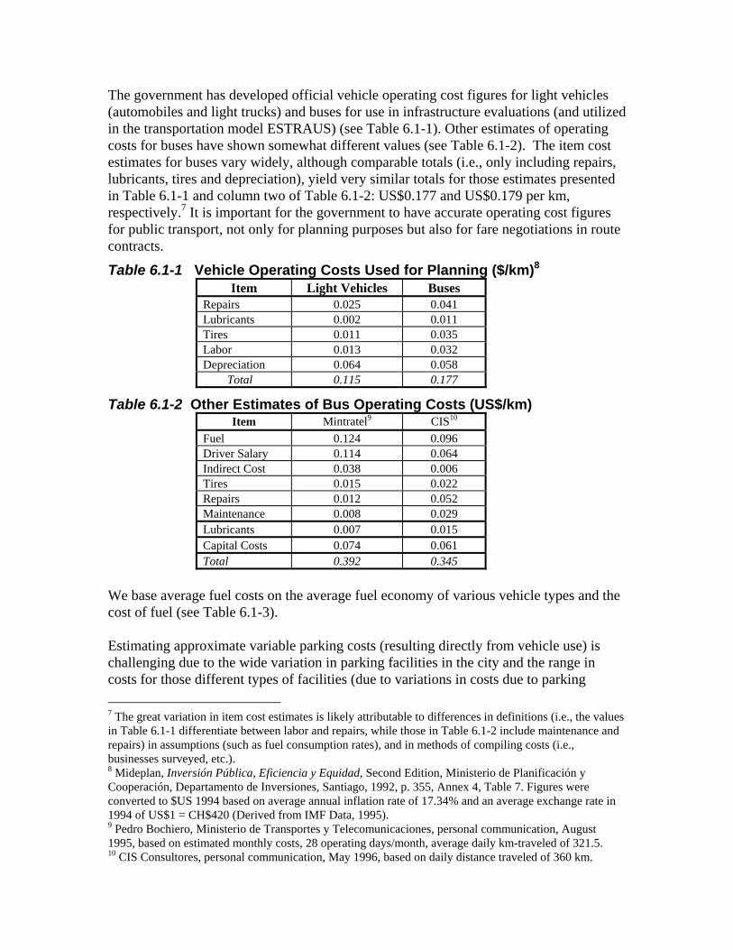
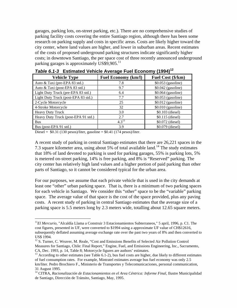
The government has developed official vehicle operating cost figures for light vehicles (automobiles and light trucks) and buses for use in infrastructure evaluations (and utilized in the transportation model ESTRAUS) (see Table 6.1-1). Other estimates of operating costs for buses have shown somewhat different values (see Table 6.1-2). The item cost estimates for buses vary widely, although comparable totals (i.e., only including repairs, lubricants, tires and depreciation), yield very similar totals for those estimates presented in Table 6.1-1 and column two of Table 6.1-2: US$0.177 and US$0.179 per km, respectively.7 It is important for the government to have accurate operating cost figures for public transport, not only for planning purposes but also for fare negotiations in route contracts.
Table 6.1-2 Other Estimates of Bus Operating Costs (US$/km) Item Mintratel9 CIS10 Fuel 0.124 0.096 Driver Salary 0.114 0.064 Indirect Cost 0.038 0.006 Tires 0.015 0.022 Repairs 0.012 0.052 Maintenance 0.008 0.029 Lubricants 0.007 0.015 Capital Costs 0.074 0.061 Total 0.392 0.345 We base average fuel costs on the average fuel economy of various vehicle types and the cost of fuel (see Table 6.1-3). Estimating approximate variable parking costs (resulting directly from vehicle use) is challenging due to the wide variation in parking facilities in the city and the range in costs for those different types of facilities (due to variations in costs due to parking 7 The great variation in item cost estimates is likely attributable to differences in definitions (i.e., the values in Table 6.1-1 differentiate between labor and repairs, while those in Table 6.1-2 include maintenance and repairs) in assumptions (such as fuel consumption rates), and in methods of compiling costs (i.e., businesses surveyed, etc.). 8 Mideplan, Inversión Pública, Eficiencia y Equidad, Second Edition, Ministerio de Planificación y Cooperación, Departamento de Inversiones, Santiago, 1992, p. 355, Annex 4, Table 7. Figures were converted to $US 1994 based on average annual inflation rate of 17.34% and an average exchange rate in 1994 of US$1 = CH$420 (Derived from IMF Data, 1995). 9 Pedro Bochiero, Ministerio de Transportes y Telecomunicaciones, personal communication, August 1995, based on estimated monthly costs, 28 operating days/month, average daily km-traveled of 321.5. 10 CIS Consultores, personal communication, May 1996, based on daily distance traveled of 360 km.
garages, parking lots, on-street parking, etc.). There are no comprehensive studies of parking facility costs covering the entire Santiago region, although there has been some research on parking supply and costs in specific areas. Costs are likely higher toward the city center, where land values are higher, and lower in suburban areas. Recent estimates of the costs of proposed underground parking structures indicate significantly higher costs; in downtown Santiago, the per space cost of three recently announced underground parking garages is approximately US$9,905.11
Table 6.1-3 Estimated Vehicle Average Fuel Economy (1994)12 Vehicle Type Fuel Economy (km/l) Fuel Cost ($/km)
Auto & Taxi (pre-EPA 83 std.) 7.8 $0.053 (gasoline) Auto & Taxi (post-EPA 83 std.) 9.7 $0.042 (gasoline) Light Duty Truck (pre-EPA 83 std.) 6.4 $0.064 (gasoline) Light Duty Truck (post-EPA 83 std.) 7.7 $0.053 (gasoline) 2-Cycle Motorcycle 25 $0.012 (gasoline) 4-Stroke Motorcycle 32 $0.010 (gasoline) Heavy Duty Truck 3.0 $0.103 (diesel) Heavy Duty Truck (post-EPA 91 std.) 2.7 $0.115 (diesel) Bus 4.313 $0.072 (diesel) Bus (post-EPA 91 std.) 3.9 $0.079 (diesel) Diesel = $0.31 (130 pesos)/liter, gasoline = $0.41 (174 pesos)/liter. A recent study of parking in central Santiago estimates that there are 26,221 spaces in the 7.3 square kilometer area, using about 5% of total available land.14 The study estimates that 18% of land devoted to parking is used for parking garages, 55% is parking lots, 5% is metered on-street parking, 14% is free parking, and 8% is “Reserved” parking. The city center has relatively high land values and a higher portion of paid parking than other parts of Santiago, so it cannot be considered typical for the urban area. For our purposes, we assume that each private vehicle that is used in the city demands at least one “other” urban parking space. That is, there is a minimum of two parking spaces for each vehicle in Santiago. We consider this “other” space to be the “variable” parking space. The average value of that space is the cost of the space provided, plus any paving costs. A recent study of parking in central Santiago estimates that the average size of a parking space is 5.5 meters long by 2.3 meters wide, totalling about 12.65 square meters.
11El Mercurio, "Alcaldía Llama a Construir 3 Estacionamientos Subterraneos," 5 april, 1996, p. C1. The cost figures, presented in UF, were converted to $1994 using a approximate UF value of CH$12616, subsequently deflated assuming average exchange rate over the past two years of 8% and then converted to US$ 1994. 12 S. Turner, C. Weaver, M. Reale, “Cost and Emissions Benefits of Selected Air Pollution Control Measures for Santiago, Chile: Final Report,” Engine, Fuel, and Emissions Engineering, Inc., Sacramento, CA, Dec. 1993, p. 14, Table 8; Motorcycle figures are authors’ estimates. 13 According to other estimates (see Table 6.1-2), bus fuel costs are higher, due likely to different estimates of fuel consumption rates. For example, Mintratel estimates average bus fuel economy was only 2.5 km/liter. Pedro Brochiero F., Ministerio de Transportes y Telecomunicaciones, personal communication, 31 August 1995. 14 CITRA, Racionalización de Estacionamientos en el Area Céntrica: Informe Final, Ilustre Municipalidad de Santiago, Dirección de Tránsito, Santiago, May, 1995.
For parking lots and garages, the space for access lanes and internal circulation increases the total land area by 1.5,15 which means a typical off-street parking space occupies approximately 19 square meters. Assuming that Metropolitan Region land prices average about $100 per square meter16 and paving costs average approximately $8.50 per square meter,17 we calculate the overall average cost of an off-street parking space to be approximately $2,000 with an annualized value of about $270 (see Appendix 1B). While the above approach significantly undervalues the cost of providing underground parking, it overvalues the cost of informal parking or parking in low land value neighborhoods. As such, we consider the average city-wide cost of a lot parking space to be a reasonable average proxy value. Not all parking is paid parking, so variable parking costs cannot be considered as a fully paid user cost (indeed, if 14% of parking in the downtown is unpaid, it is fair to assume that -- at a minimum -- the inverse is true in non-central areas, i.e. 14% or less is paid). In the case that variable parking costs are unpaid, this cost is not perceived by users (thus does not affect travel decisions18), instead it remains an external user cost (paid by society). This external cost can take various forms, such as higher prices for goods sold at places where free parking is provided (i.e., shopping malls) or disruption of social-spaces such as sidewalks, greenspaces, etc. occupied by parked vehicles.19 We estimate that, city-wide, approximately 60% of variable parking costs (workplace, shopping, other) are unpaid and that about 20% of variable parking occurs on existing roadspace/alleyspace (an estimated 55,500 spaces).20 To avoid double counting, we subtract the cost of these spaces from the facility costs estimated in Sections 6.5 and 6.6 (see Appendix 1B). For the metro, we consider variable costs to be energy, maintenance, depreciation, personnel, and other general expenditures; for motorcycles we consider variable costs to be 40% of automobile operating costs (according to Table 6.1-1), 1/4 automobile parking
15CITRA, Racionalización de Estacionamientos en el Area Céntrica: Informe Final, Ilustre Municipalidad de Santiago, Dirección de Tránsito, Santiago, May, 1995, p. 17. 16Derived from Associacion Gremial de Corredores de Propiedades (ACOP), "Informe Estadistico Trimestral: Analysis de la Oferta de Sitios y Relacion Precio Oferta v/s Precio Venta Real en 34 Comunas de Santiago." Four Volumes: Jan-March 1994, pp. 74-75; April-June 1994, pp. 78-79; July-Sept. 1994, pp. 75-76; October-Dec. 1994, pp. 72-73. See also, Appendix 2. 17CITRA, Racionalización de la Problemática de Estacionamiento en la Principales Ciudades del Pais: Informe Final, Ministerio de Transportes y Telecomunicaciones, Departamento de Transporte Urbano, June 1995, p. 4-5. 18 Although the anticipated hassle (non-market cost) of having to try to find a parking place in a saturated zone definitely does affect travel decisions. 19 Parking on sidewalk facilities, beyond occupying public spaces imposes additional externalities of travel time delay for pedestrians, increased rate of pedestrian facility degradation, and increased accident risk for pedestrians that have to step into the street to avoid parked vehicles. 20 In the case of on-road, un-paid parking, the cost of providing this parking space is paid by transport system users at large (assuming user charges completely cover facility costs, which we discuss in Chapters 6.6 and 6.7). In this case, on-road parking is subsidized by other transport system users. This results in a sub-optimal use of roadspace (decrease in design capacity) and over-design of parking facility (roads are designed with more demanding specifications than that needed for parking).
costs, with fuel costs as listed in Table 6.1-3. For bicycles we consider variable costs to be $20 per year for maintenance, and 1/7th of the variable parking costs for automobiles without paving costs (see Appendices 1A and 1B). For pedestrians, we consider that walking wears out shoes at the rate of $0.005 per kilometer. Fixed Costs The cost of an automobile varies widely, depending on make, model, accessories, and government imposed fees. For estimating approximate vehicle ownership costs, we use the average cost of a 2000 cc automobile, as summarized in Table 6.1-4.
Table 6.1-4 Typical Automobile Purchase Costs (U.S. Dollars) Engine Capacity: 1500 cc 2000 cc 5000 cc
Total 8,513 13,403 91,808 Annualized Capital Cost21 $1,433 $2,257 15,462 We use the same vehicle purchase cost for light trucks and assume the average motorcycle costs one tenth the cost of a car. We assume a bicycle costs $200 and that an average bus costs about $144,000. Taxis and colectivos are assumed to have the same purchase costs as an automobile. For all vehicles, we translate purchase costs into annualized cost, assuming straight line depreciation, life time of 11 years, and an interest rate of 12%. Motor vehicle owners incur the following additional annual costs: 1. Annual registration fees (permiso de circulación). The permiso de circulación is an
annual fee collected by the individual Municipalities which essentially serves as a general revenue generator and as an income redistribution mechanism. The Municipalities dedicate 50% of the revenues from permisos de circulación to the Municipal Common Fund (FCM).22 This fee ranges from 1% of assessed value for vehicles worth less than $2,700 up to 4.5% of assessed value for vehicles worth more than $18,000, and averages about $121 annually. Taxis, buses and colectivos pay approximately $50, trucks pay according to weight. Registration fees are an important source of Municipal revenues. Even after the portion dedicated to the FCM, permisos
21 Assuming straight line depreciation at 12% interest over estimated vehicle lifespan of 11 years. 22The Chilean Government created the Municipal Common Fund (Fondo Común Municipal or FCM) in 1991 as a mechanism to redistribute income between Municipalities in the country. Originally, the FCM was distributed accordingly: 10% in equal part to all Municipalities; 20% according to the number of residents; 30% according to the amount of tax-exempt land; and 40% according to the per capita municipal revenue. In 1995, the distribution of the FCM was changed accordingly: 10% in equal parts, 15% according to population, 10% according to relative poverty, 30% according to tax-exempt land, and 35% according to per capita municipal revenue; the other 10% is disributed in part according to municipal efficiency and the rest for emergencies (from: Ecomuna, "Pobreza, municipio, y medio ambiente," CIPMA, Santiago, Dec 1995, p. 1. created by the 20% for Providencia, 13% for San Bernardo, 6% for San Joaquin,
de circulación provided 20% of total revenues for Providencia, 13% for San Bernardo, and 6% for San Joaquin.
2. Insurance. Vehicle owners are required to purchase liability insurance costing
approximately $20 per year. Approximately 80% of drivers carry only this insurance. Vehicle owners who do purchase comprehensive liability and collision insurance typically pay about $1,200 per year. Buses pay approximately $200 per year.
3. Safety and Emission Equipment Inspections. Inspections at government authorized
centers ensure the effective operation of vehicle emission control and safety equipment, including lights, brakes, and safety belts. Automobiles are inspected annually, buses and trucks are inspected every six months. This service costs $5 to $7 per inspection for automobiles and for buses approximately $12. Buses must have emissions inspections every three months, at a cost of $7. Starting in 1996 automobiles with catalytic converters will only require inspections every other year.
4. Parking Costs. The annual parking cost that is paid as a fixed cost by users is
essentially the cost of vehicle storage (i.e., parking at home for private vehicle owners, and parking facilities for buses, taxis, colectivos, and metro). The cost of this parking space is estimated in the same way as that for variable costs described above. Again, this cost varies according to type of parking facility: some people have personal parking spaces in underground garages, some in driveways, while many end up parking on streets or informally on sidewalks and front lawns. In apartment buildings, the cost of a parking space is typically included in rent charges, while in private homes, driveway parking space cost is the opportunity cost of the occupied land. In either case the cost is internalized (although the homeowner rarely considers the annual cost of maintaining his/her parking space). We assume that 8% of all fixed parking costs are informal (on streets, alleys, or sidewalks), which is a non-user paid cost, picked up by society at large. Again, to avoid double counting, this on-road fixed parking cost is subtracted from road facility costs in Sections 6 and 7 (see Appendix 1B).23
Cost Summary Based on the cost estimates described above, we estimate average automobile fixed costs (annual capital costs, registration, insurance, parking and inspections) to average approximately $2,400 per year. For a vehicle driven 15,000 kilometers a year, this averages about $0.16 per kilometer (see Table 6.1-5). Variable automobile costs average about $0.115 per kilometer, or about another $1,725 per year. Variable costs for an average light truck are slightly higher (due essentially to higher fuel costs). The fixed costs for a motorcycle are about $308 per year ($0.02 per km) and the variable costs average about $0.04 per km. We estimate the fixed cost of an average bicycle at $58 per year, or about $0.01 per km and the variable costs at about $0.008 per km or about $47
23 While vehicle parking on pedestrian facilities is a common phenomena in many parts of the city, we do not attempt to estimate what number of vehicles park in these facilities and do not subtract out those costs from pedestrian facility cost estimates in Sections 6 and 7.
per year. Our pedestrian costs are based simply on increased rate of wear on shoes and are completely variable (assuming people would have shoes whether they travelled or not). For bicycle and walking we do not consider the potentially increased food costs needed to fuel these modes.24 Variable costs will be slightly higher under peak period conditions due to increased wear and tear from stop-and-go travel.
Table 6.1-5 Ownership and Operating Costs per Vehicle Kilometer Variable Costs
Figure 6.1-1 Composition of Private Vehicle Ownership and Usage Costs25
0%
10%
20%
30%
40%
50%
60%
70%
80%
90%
100%
Avg. Auto Avg. LightTruck
Avg.M otorycle
Variable Parking
Tires, M aintenance, etc.
Fuel Costs
Capital Costs
Fixed Parking
Registration, Insurance,Inspection
24 Most people now seem to perceive a benefit from burning off calories through exercise. 25 For derivation of these percentage breakdowns see Appendix 1A.
Table 6.1-6 Ownership and Operating Costs per Passenger Kilometer Variable Cost
(US$ per PKT) Fixed Cost (US$ per PKT)
Total Cost (US$ per PKT)
Walk 0.005 0.000 0.005 Bicycle 0.008 0.01 0.018 Pre-EPA Auto 0.081 0.107 0.188 Post-EPA Auto 0.074 0.107 0.181 Pre-EPA Light Truck 0.089 0.107 0.196 Post-EPA Light Truck
0.082 0.107 0.189
Pre-EPA Bus 0.005 0.011 0.016 Post-EPA Bus 0.005 0.011 0.017 Pre-EPA Taxi 0.069 0.130 0.199 Post-EPA Taxi 0.062 0.130 0.192 Pre-EPA Colectivo 0.035 0.081 0.116 Post-EPA Colectivo 0.031 0.081 0.112 2 Stroke MC 0.041 0.021 0.062 4 Stroke MC 0.038 0.021 0.058 Metro 0.054 0.000 0.054 For private vehicles (automobiles and light trucks), about 50% of ownership and usage costs are annualized capital costs of vehicle ownership; six percent are estimated fixed parking costs; other fixed ownership costs (insurance, registration, inspections) combined make up about three percent of costs. For a vehicle driven an average 15,000 km per year, fuel costs comprise about 17% of total costs and operating and maintenance costs comprise another 17% of costs. The remaining 6% of costs are estimated variable parking costs (see Figure 6.1-1). In summary, about 60% of user costs are fixed costs, the remaining 40% are operating costs. When examined on cost per passenger kilometer travelled, based on average vehicle occupancy rates, we can see that the operating costs for automobiles, taxis and light trucks are in the same cost range, nearly $0.20 per passenger kilometer travelled (pkt). An average bicycle costs less than $0.03 per pkt, a motorcycle trip about $0.055 per pkt and a walk trip less than one U.S. cent. It is important to note that these cost estimates include parking costs, whether they are actually paid or not. Based on our admittedly crude estimates of total parking costs and estimated portion of paid fixed and variable parking costs, approximately 60% of variable parking costs go unpaid by users and approximately 8% of total fixed parking costs go unpaid by users.26 According to these estimates, unpaid parking in the city is valued at some US$88 million per year (see Appendix 1B). In other words, the owner of an average automobile owner who never pays for variable parking (i.e. at work or shopping) receives a parking subsidy of approximately $270 per year. For this unpaid
26 Much fixed parking costs are not recognizred as “paid” by users who maintain parking spaces on their property. All subsidized, or unpaid, fixed parking costs occur as on street parking.
variable parking costs, the question of who provides the subsidy depends on where the parking occurs. For example, in the case of on-street parking, the parking is paid by other system users or taxpayers in general (depending on whether road user charges fully cover infrastructure costs, which is examined later in this report). In the case of free retail parking, for example, this cost is subsidized by all retail shoppers (through higher goods prices).27
Trends and Implications These cost estimates have interesting implications for current and future transport system performance and pricing policy. For example, according to the cost per passenger kilometer ($0.017) for bus operation (assuming average vehicle occupancy rate of 30 passengers), a bus trip of approximately 15 to 16 kilometers covers the full operating cost related to the trip. Shorter trips subsidize longer trips, with the size of the subsidy proportional to the distance traveled (see Figure 6.1-2). Additional subsidies are provided by regular bus users to student users (who pay approximately 1/3 the regular fare). It is not clear why -- if the government determines that students’s fares should be subsidized -- that subsidy should be payed by public transport users. Furthermore, considering that student trips account for a large portion of peak period trips (for example, between 7:30 and 8:00 a.m. during the morning peak school trips account for over 60% of all trips and the majority of motorized school trips occur on bus28), it seems likely that this pricing policy overburdens the already saturated peak-period capacity of the bus system.
27 These external costs of parking do not include air pollution, traffic congestion caused by the reduced road capacity due to on-street parking, and the contribution of parking to urban sprawl. A study of parking in downtown Santiago estimates that the daily external cost of a parking space in the central city is about $0.26 for a space in a parking garage, $0.70 for a space in a parking lot, and an average $0.50 per on street parking space (Derived from CITRA, Racionalización de Estacionamientos en el Area Céntrica: Informe Final, Ilustre Municipalidad de Santiago, Dirección de Tránsito, Santiago, May, 1995, pp. 19-20, Tables 3.3-2, 3.3-3, and 3.3-4.) 28 In 1991. From SECTRA, Encuesta Origen Destino de Viajes del Gran Santiago 1991, Santiago, 1991, pp. 23, 30.
Figure 6.1-2 Bus Passenger Payments and Costs as Function of Distance
0
0.05
0.1
0.15
0.2
0.25
0.3
Distance (KM)
US$
Shorter TripSubsidy to
LongerTrips
Size of Subsidy toLonger Trips
Increases with TripLength
Approximate Break-Even Point (Fare
Paid equals Cost ofProviding Trip)
Curve Represents Cost per kilometer, paid byregular bus passenger in 1994
Line Represents AverageCost per pkt, experienced by
For bus system pricing, these cost estimates suggest that distance-based pricing should be introduced, so that users pay the full marginal cost of their travel decisions (thereby eliminating or reducing the cross-subsidies shown in Figure 6.1-2). This will likely carry important equity impacts, since the majority of the longer trip-makers are likely low-income users. To mitigate this adverse impact on low-income users, the government should introduce another, more targetted, subsidy mechanism -- such as a travel stipend for certain income groups. This would ensure that low-income users, forced to live in distant suburbs (due to the historical policy of building public housing on the cheapest possible land) would still be guaranteed a minimal level of mobility. In addition, since the cost of bus operation likely increases during peak periods, due to increased operating costs of stop-and-go traffic, peak period pricing should also be introduced into the bus system (similar to that introduced in the Metro system). Based on the estimates presented here, passenger transportation ownership and usage costs in Santiago amounted to nearly $3.4 billion in 1994,29 or approximately 17% of Gross Regional Product (see Appendix 1C).30 Approximately, $88 million of those costs are external, unpaid parking costs. As elsewhere throughout the world, the average cost of owning an automobile is high, but operating costs are relatively low and declining, due to declining international
29 Includes bus, taxi, colectivo, Metro, walking, autos, bicycles, pickups (see Appendix 1C). Also this includes parking costs, even those costs not necessarily financially transzcted (i.e., the opportunity cost of land homeowners dedicate to vehicle storage). 30 This estimate is consistent with other estimates in Chile of transport as a share of total household spending on goods and services, estimated at 17% in 1988 (see Escudero & Lerda, op. cit. 1).
petroleum costs and increased fuel efficiency among newer vehicles. Nonetheless, based on the variable operating costs (fuel costs and additional operating and maintenance costs) estimated here an automobile trip in Santiago is significantly more expensive than a bus trip. Consider, for example, a 15 kilometer commute, without any parking charges at the end. For a post-EPA vehicle (with a fuel efficiency estimated at about 10 km/liter), this trip costs nearly US$ 1.40, one way. The same trip on a bus in 1994 would cost about US $0.26, or about five times less. Add an additional $1.50 for parking,31 and an auto commute trip to the downtown costs almost 11 times as much as a bus trip. This cost difference does not include any ownership or depreciation costs for the automobile user. An automobile trip becomes more financially competitive with a bus trip once auto occupany rates increase (assuming operating costs are shared among all occupants). For example, if the same commute trip considered in the preceding paragraph carried four occupants, then the cost per occupant decreases to about $0.35 per passenger, not including parking. Despite the straight financial advantage that public transport offers, trends in Santiago indicate that, at first opportunity, most travellers in the city switch to private motor vehicles for most of their trips. This is due primarily to the real and perceived time advantage that private motorized travel offers, as well as other important influencing factors such as comfort, status, flexibility, and security. Some of these factors will be discussed and quantified in the following section. The continued growth in automobile use is likely to increase the total amount of money spent by all users on transportation. Increased automobile use can also lead to increased transit fares, due to greater congestion delays and lost economies of scale for transit. In addition, if urban outgrowth occurs in the auto-dependent form it is currently taking, then the bus system will face a series of difficult choices: • increase the level of cross-subsidy from short distance passengers to long distance
passengers, thereby running the risk of losing short distance passengers to competing modes;
• abandon suburban bus service or severely cut-back suburban routes (currently impossible given current route structuring, where routes run from one extreme of the city to the other);
• directly subsidize bus service (which is virtually impossible in the current political climate and will likely result in the service inefficiencies prevalent in many highly subsidized bus systems);
• work to promote more bus-friendly urban development patterns (incorporating so-called neo-traditional development or new-urbanism design principles).
• work to specifically increase the speed of bus service (exclusive facilities), the status of riding the bus (information campaigns), the reliability of bus service, the comfort and convenience, and the productivity of time spent in bus travel.
• introduce variable, distance-based pricing mechanisms. 31 Estimated all day parking in paid parking space is approximately $3.00, attribute evenly to both sides of the work trip.
This last option seems the most rational from an economic perspective and may even help contribute to more transportation efficient land development in the medium-term. Without moving towards some form of marginal cost pricing for the bus system it seems likely that the general fare convergence and consistency achieved in recent years (see Figure 6.3-3)32 will either be lost (as bus fares are forced upwards to account for increasing operating costs) or system subsidies will become necessary.
Figure 6.1-3 Evolution of Public Transport Fares (US$ 1994)
0
0.05
0.1
0.15
0.2
0.25
0.3
0.35
0.4
1985 1986 1987 1988 1989 1990 1991 1992 1993 1994
Metro Line 1 Metro Line 2 Bus
The continuous growth in automobile ownership also has important implications for the user cost of parking provision and relevant policies in Santiago. With approximately 500,000 private automobiles currently registered in the city, an additional 1,000,000 parking spaces will be needed over the next decade to meet the increased demand created by a 10% annual growth rate, assuming that each vehicle requires an average of two spaces. Some of these additional parking spaces will be provided voluntarily by vehicle owners at their residences and by businesses happy to satisfy the needs of their customers and employees. But there are sure to be problems, particularly over access to publicly owned parking spaces (both on- and off-street) and informal parcels of land suitable for parking a motor vehicle. In addition, the provision of free or underpriced parking represents a subsidy of driving that imposes unfair costs on taxpayers, business customers and employees who don’t drive (because they pay a share toward the cost without receiving direct benefits). The existing supply of parking spaces (including informal parking spaces such as curbs and vacant lots) is already heavily used. Providing sufficient parking capacity will require many more parking spaces and increasingly expensive facilities as the available supply of land is exploited. At least in part due to these pressures, some municipalities in the city have announced plans for construction of a series of underground parking facilities, especially in downtown Santiago as well as in some of the more highly motorized municipalities like Las Condes and Providencia. In general, these underground 32Derived from Metro, S.A. Informe Anual,"Caracteristicas de la Red," p. 55. The fares were adjusted for CH$1994 according to inflation rates for the years 1985-1994 from IMF. For years when the fare varied, the median was used. For 1994, when differentiated fares for the Metro were introduced, the normal fare was used. The variation in Line 2 fares is due to changes in policy regarding fare integration with Line 1; in 1989, the transfer charge was eliminated, in 1991 it was re-instated, and in 1992 it was eliminated again.
facilities will help internalize a large portion of total parking costs, not only because users will be expected to pay the full construction and operating costs (since the structures will be privately built and operated), but also because by being completely underground, these structures will reduce the total surface area of the city dedicated to transportation (thereby minimizing parking's sprawl effects). Nonetheless, there is a need to move towards more rational motor vehicle use (and ownership) through direct marginal cost parking charges for all parking spaces. While the most recent Master Plan for Santiago (1994), established minimum parking requirements for various types of land uses (ranging from apartment buildings to hospitals, to schools), there is no consideration in the Plan for parking charges.33 Without effectively charging for parking provision, owners do not absorb the full costs of their decision to purchase a vehicle (for example, if they can then park it for free on the street), and users do not pay the full costs of their decision to travel. The result is approximately $88 million in un-paid parking costs in the city. To improve this situation and send proper pricing signals to users, all parking provision should be charged. For on-street residential parking, this could be achieved through annual parking permits sold by municipalities, based on annualized facility costs. Illegal parking on medians and sidewalks should be tightly enforced and penalized. Authorities might consider the policy adopted in Japan, whereby new vehicle purchasers must show evidence of having parking facilities. For variable parking at malls, retail sites, work-places, etc., parking charges should also be mandated, not simply offered free with the cost absorbed by all other consumers. Establishing such charging mechanisms could also open the door to use parking charges as a proxy congestion charging tool -- variable parking charges could be higher for vehicles that arrive during peak travel periods.
33For example, large homes (over 150 square meters) must provide a minimum of two parking spaces. Parking requirements for office building range from 1 for every 30 square meters of parking space in highly motorized areas to 1 for every 100 square meters in less motorized parts of the city (MINVU, Plan Regulador Metropolitano de Santiago, Santiago, October 1994, pp. 125-130.).
6.2 Travel Time Costs The value of travel time includes the cost to travelers of unpaid time or the cost to employers for work time spent in travel, the cost to society in general for potential productive time spent traveling and the cost to commercial interests for shipping times for goods (or services) delivery. Travel time costs are typically measured as a function of wage rates and can vary according to trip purpose,1 trip-maker (i.e., student, retiree, worker), and travel mode. Of transportation costs, travel time costs have been perhaps the most widely studied and measured; travel time savings, after all, are one of the primary rationales for transportation project enhancements. Of the traditionally quantified benefits and costs of transportation analysis, travel time remains as perhaps the most controversial, because of debates over both how travel time should be valued and how travel time should be measured (i.e., as reported by users, predicted in models, or actually measured on the network).2 In the planning, evaluation, and actual performance of transportation systems, travel time values can actually be differentiated along at least two lines -- private travel time costs that individual users experience and social costs of travel time (the value of that time to society). Private travel time costs are often referred to as perceived, or subjective measures of travel time. They do not necessarily represent the actual amount of time one spends traveling, rather they reflect the individual's subjective interpretation of that time. Behind these measures is a long evolved application of micro-economic theory, treating individuals' travel decisions as a rational allocation of time resources to maximize benefit (utility) given certain constraints.3 By placing a value on time, we are simply trying to develop a common denominator to help understand and explain individuals' time allocation choices. For example, if an individual chooses to work one less hour per week to share that hour with a friend, we can say that that individual values that hour with a friend at, at least, his/her individual hourly wage. Transportation planners trying to predict transportation system performance are most concerned with perceived, or subjective, measures of travel time. In this sense, travel time values are used to establish a level playing field, from which trip times in various modes, under different conditions can be measured. For example, although a complete bus trip and a complete automobile trip might have the same actual time, the bus trip may be viewed by the traveler as costlier than an auto trip, due to waiting time, crowded
1 For example, the value of time spent for a work trip is typically valued higher by individuals and society than the value of time for a shopping or recreational trip. 2 David Hensher, "Value of Travel Time Savings in Personal and Commercial Automobile Travel," Draft paper prepared for a Conference on Social Cost-Benefit Analysis, sponsored by U.S. Bureau of Transportation Statistics, held at University of California-Irvine, July 1995, p. 2. 3 A good overview of the theory of valuing travel time and a summary of empirical studies is contained in K. Small, Urban Transportation Economics, Harwood Academic Publishers, (Chur), 1992, pp. 36-45.
conditions, etc.4 In this sense the user's travel time cost by bus is higher than that by car.5 This perceived travel time cost helps explain, for example, why travelers opt for traveling by automobile even when it is financially costlier than bus travel (as shown in the previous Section 6.1). While in some cases the auto trip might offer real travel time savings, some of those time savings might actually be perceived -- waiting for the bus seems longer than it actually is, standing in uncomfortable conditions makes a trip seem longer than it is. Variations in subjective travel times are multiple: walking or bicycling trips may have a low travel cost if the conditions are favorable (safe, quite, non-polluted), but might increase sharply after certain "threshold" distances. Further differentiation can occur according to income level, trip purpose (travel time costs for recreational purposes might be lower than for work trips), gender, etc. It is even possible that some trips have negative travel time cost (i.e., trips made exclusively for pleasure, such as recreational bicycle trips). This perception of travel time is important for modelers to predict how travelers will respond to various travel conditions or newly introduced travel options. For example, making wait time for transit less un-predictable by providing schedule information or real-time travel time updates (now possible through advanced vehicle tracking systems) could reduce the perceived travel time for transit and increase its attractiveness. Perception of travel time is also important for decision-makers and politicians. Since individual travel time values increase substantially with congested driving conditions (not just the additional time lost in traffic, but the increasing value of that time to the increasingly frustrated traveler), politicians consider reducing this perceived cost to users as critical to keeping voters (users) happy. The main problem with using private travel time values in transportation analysis and decision-making comes from their wage-based derivation and potential subsequent social equity impacts. While individual values of travel time can show us how much a specific individual is willing to pay (in time) to take a certain trip (on a certain mode, for a certain purpose), they will not necessarily show us how much society should be willing to pay (for that time). For example, a wealthy worker might personally value a five minute reduction in a congested morning auto commute greater than a poor worker might value the same reduction in bus travel time. If these time values dictate public investment decisions, then the result may emphasize travel time savings for wealthier travelers. Because of the equity implications of this situation, as well as the fact that individual value of travel time savings might not equal socially-optimal travel time values, planners most often use a single average wage rate to value travel time savings. Social travel time values are, thus, based on time value functions derived from private time savings values, but adjusted for equity considerations based on average earnings. This remains as the 4 Other factors, such as perceived status among peers, might also increase travel time costs for one mode versus another. 5 Of course, the opposite might also hold true: a bus trip might have lower time costs for travelers who appreciate the time on a bus as free time.
most credible approach to socially valuing travel time savings, since time allocation is an extremely individual decision-making process. Consequently, time savings are indicated as a percentage of average wages, varying according to type of travel, type of traveler, and, sometimes, travel conditions, mode, and level of congestion. An example of a travel time schedule is shown in Table 6.2-1.
Table 6.2-1 Example of Travel Time Values6 Travel Time Values Commercial vehicle driver Wage rate plus fringe benefits Personal vehicle driver 50% of current average wage Adult car or bus passenger 35% of current average wage Child passenger under 16 years 25% of current average wage Congestion increases travel time costs for drivers by the following amounts according to Level of Service (LOS) ratings:
LOS D: multiply by 1.33 LOS E: multiply by 1.67 LOS F: multiply by 2.0
Cost Estimates In Chile, much research over the past decade has focused on developing appropriate travel time values for use in inter-city and urban transportation planning. Particular emphasis has been placed on the relatively unique labor and travel characteristics of a developing country (such as Chile), especially: wide differences in individual's socio-economic characteristics, the traits of the Chilean labor market, and in travel conditions of various modes. In recent years, as part of a nationally funded effort, a combination of revealed and declared preference surveys have been used to develop a more accurate range of time values to be used, stratified according to income levels, trip type, occupation, etc.7 Unfortunately, the results from this research, to-date, have shown a high degree of uncertainty and show that much work remains to better define working values.8 As such, travel time values that continue to be utilized for planning in Chile are derived from values used in industrialized countries and are measured as a fixed portion of average hourly salary (see Table 6.2-2). It is typical practice in Chile to value wait time 1.5 times greater than in-vehicle time and walk and bicycle time at 2 times greater than in-vehicle time.9
6 The Value of Time Savings for The Economic Evaluation of Highway Investments in British Columbia, Dr. W. Waters, British Columbia Ministry of Transportation and Highways (Victoria, B.C.), March 1992. 7For a review of this work see MacroIngenieros, "Analisis Metodologia de Vector de Precios Sociales en Estudios Viales: Informe Final," Ministerio de Planificación y Cooperación, December 1994 (Santiago), December 1994, pp. 3-16 - 3-20. 8MacroIngenieros, "Analisis Metodologia de Vector de Precios Sociales en Estudios Viales: Informe Final," Ministerio de Planificación y Cooperación, December 1994 (Santiago), December 1994, p. 3-20. 9 Mideplan, Inversión Pública, Eficiencia y Equidad, Second Edition, Ministerio de Planificación y Cooperación, Departamento de Inversiones, Santiago, 1992, p. 338.
Table 6.2-2 Value of Travel Time Used in Planning in Chile10 Type of Traveler Percent Average Wage Cost Per Hour11
Employed Adult 50.0% $1.25 Other Adults 48.5% $1.21 Retired People 33.5% $0.84 Students (under 18) 12.5% $0.31
Table 6.2-3 Estimated Trip Characteristics in Santiago (1991)12 Mode Reported Trip
Times in Minutes Estimated Off Peak
Travel Speeds (KM/h)
Estimated Peak Travel Speeds
(KM/h)
Total Trip Distance
(KM) Auto 25.7 40.9 22.5 13.38 Pickups 25.7 40.9 22.5 13.38 Bus 45.2 30.7 16.9 13.33 Taxi 22.6 40.9 22.5 10.58 Colectivo 28.6 36.8 20.2 11.35 Motorcycle 25.7 40.9 22.3 11.26 Metro 29.3 32 32 9.71 Walk 18.3 5 5 1.44 Bicycle 33.2 15 15 8.05 To determine cost of travel by different modes in Santiago, we use travel times for the various travel modes as reported in the 1991 origin destination survey.13 It is important to note that these travel times are based on user reported travel times (people’s response to travel survey questions) and may not reflect actual travel times as measured directly in the system. In this sense, the reported measures might already reflect the higher travel time costs associated with waiting, walking, congestion, etc.14 According to the survey results, average trip times estimated for Santiago on all modes, over the entire day range from 32.5 minutes in the northern part of the city to nearly 39 minutes in the center of the
10 Ibid., p. 355, Annex 4, Table 8. 11 Based on US$ 2.50 per hour average wages. 12 Reported trip times from Comisión de Planificacción de Inversiones en Infraestructura de Transporte, op., cit. pp. 15-81 - 15-86. Again, note that these are survey results based on travelers' reported trip times. Pickup trip and motorcycle time is assumed same as auto, bicycle trip time is taken as that of "other". We do not include the wide range of inter-modal combinations (i.e., bus-metro, taxi-metro) reported in the survey. For derivation of estimated peak and off-peak travel speeds see Appendices 3-3A. Travel speeds for private vehicles, including taxis, are reportedly derived from ESTRAUS as cited in Departamento de Estudios Económicos, " Memorandum: Costo Social por Congestión de Tránsito en el Gran Santiago," Camara Chilena de la Construcción, Santiago, Sept., 1993, Table 6. Travel speeds for buses are estimated at 75% of private vehicles and colectivos 90% and each is estimated to suffer the same congestion penalty as private transport (i.e., peak travel speed is 55% of off-peak speed). Metro average vehicle speeds are those reported by Metro (see Appendix 7C), bicycle and walk speeds are authors' estimates. Total Trip Distance includes access and egress to public transport (including taxis and colectivos). See, also, Appendice 3-3A. 13 Due to lack of data, we do not consider freight or other commercial traffic in this analysis. 14 As such, adding travel cost "penalty" to these modes or travel conditions might constitute double counting.
city.15 The average time for an automobile trip was nearly 26 minutes, for a bus trip 45 minutes, a taxi trip nearly 23 minutes, colectivo and metro 29, and walk about 19 minutes (see Table 6.2-3). Using the average daily travel times reported in Table 6.2-3, average network speeds, and estimated access/egress and wait times for various travel modes, we estimate travel costs per passenger kilometer traveled as reported in Table 6.2-4. The methodology used to derive these costs are detailed in Appendices 3 and 3A. These costs may be underestimates, since travel times may well have increased over the period 1991 to 1994.
Table 6.2-4 Estimated Travel Time Cost by Mode in Santiago16
Mode $/Trip $/PKM Auto 0.58 0.05Pickups 0.58 0.05Bus 1.00 0.09Taxi 0.49 0.05Colectivo 0.63 0.06Motorcycle 0.48 0.05Metro 0.64 0.07Walk 0.76 0.53Bicycle 1.38 0.17 According to these estimates, private personal vehicles offer (autos, pickups, and motorcycles) the least costly travel option, followed by taxi, colectivo, metro and bus (see Table 6.2-4). A bicycle trip is over three times as costly as a auto trip and a walking trip is nearly 11 times as expensive (in terms of $ per passenger kilometer). It is necessary to highlight that these cost estimates are for a typical employed adult's work trip. For student trips, trips by non-employed working age adults, or retirees, the costs would be proportionally less.17
Trends and Implications Some important points should be noted when comparing these numbers. First, these cost estimates assume that people in Santiago find walking and bicycling to be extremely unpleasant (twice as costly as travel in motorized vehicles). While this may well be the case for very long trips by these modes, this is unlikely the case for shorter trips, which many travelers might view as pleasant (i.e., low cost). These costs could be significantly lowered by improving the environment within which these modes are used as well as by shortening total trip distances. 15 Comisión de Planificacción de Inversiones en Infraestructura de Transporte, Encuesta Origen-Destino de Viajes del Gran Santiago 1991: Informe Final, Volumen III, MIDEPLAN, Santiago, August 1992, p. 15-81, Table 15.52. 16 For Derivation of these costs, see Appendices 3-3A. 17 The proportion should, in theory, be the same as those presented in Table 6.2-2, although trip characteristics for non-work trips might be different (i.e., shopping trips might be longer or shorter according to various modes).
For existing non-motorized trips, this signifies that the government should take measures to improve safety through traffic calming on local streets and secure and dedicated facilities on more dense travel corridors. Additional environmental improvements, such as reductions in air and noise pollution, bring synergistic benefits here, by making these non-polluting modes more attractive, increasing their use, and further reducing pollution (a so-called "virtuous cycle"). To promote increased use of these non-motorized modes for future trips (generated by new urban development), these costs signify that development should occur at density levels that allow reasonable walk/bike distances, within environments that make travel by these modes pleasant. With respect to public transport trips, these are twice as costly as private vehicle trips (in terms of $ per passenger kilometer). This is due in part to slower travel speeds, longer access and egress times, and wait times (which receive a cost penalty, 1.5 times greater than travel time cost).18 However, in spite of the higher travel time costs of a public transport trip, the overall user-experienced cost of a public transport trip -- considering the financial costs derived in Section 6.1 -- still does not approach that of a private vehicle trip. As estimated in the previous section, a typical automobile commute has direct financial costs nearly five times higher than a bus trip (not including auto parking costs): US$ 1.40, one way versus US $0.26 for a bus trip. Incorporating the travel time costs derived here makes the balance nearly $2.00 for an auto trip and $1.26 for a bus trip. If an automobile trip remains more costly than a bus trip -- even when taking into account travel time costs -- there must be other factors, not included in these cost accounts, that are influencing the rapid ascension to private vehicle trips when the economic opportunity presents itself. Some of these factors were presented in a study done for the Chilean Ministry of Transport in 1995. Based on focus groups with middle income automobile users, the study found particular qualitative characteristics that made individuals prefer auto use instead of public transport use, including: door-to-door availability, assured seating, space to carry personal items, music of choice, privacy (or at least selection of travel companions), and air conditioning.19 Participants in the survey went further to delineate particular characteristics of public transport use that were considered to be "reductions in personal liberty," including having to accept decisions of the driver in terms of speed and route and having to endure the presence of odors, sounds, and other factors (in particular, singers and vendors which are typical on buses in Santiago). These "reductions in personal liberty" were contrasted with the "expansion in personal liberty" that participants associated with the auto.20 These qualitative characteristics clearly translate into economic value that sways individual trip-making decisions. To get a general idea of the value of these qualitative 18 These cost estimates do not give in-vehicle public transport travel time a higher value than private vehicle travel time. 19 "Actitudes y Motivaciones Ligadas al Uso de Automóvil Particular v/s Transporte Público: Estudio Cualitativo," prepared for the Ministry of Transport, February 1995, p. 8. 20 Ibid., p. 14.
characteristics, we can return to the example used in the previous Section 6.1. A fifteen kilometer commute trip combined with parking charges costs approximately $2.90 in direct user variable costs, with an additional $0.75 in travel time costs, or approximately $3.65. The same bus trip incurs financial and time costs of about $1.60, less than half of the auto trip. One interpretation of this difference could be that a typical automobile commuter values the "increases in personal liberty" that an automobile brings at at least $2.05, or nearly $0.14 per kilometer. Recognizing the qualitative value that an auto trip brings to users is important if policy-makers consider prioritization of public transport as a key transport policy goal, as they ostensibly do in Chile. If prioritizing public transport means making it competitive with auto-based alternatives, then the estimates here have two implications for public transport development. One is to improve public transport system performance to make its actual time costs more competitive with those of private modes. This can be achieved by reducing walking distances to bus stops (transit-oriented development); reducing the wait time and/or perceived wait time for bus and Metro (which can be accomplished through improved waiting facilities, clear and accurate bus-scheduling, and real-time transit information); and reducing the actual in-vehicle travel time (by dedicated bus facilities and bus prioritization at intersections and increased Metro frequency and train size). A second implication of these estimates for public transport policy is the need to develop road-based public transport that can compete with the qualitative benefits that users associate with the auto. If public transport could begin to offer the same qualities that auto users currently enjoy, then perhaps public transport service can recapture some of its lost market share and prevent further market erosion. Our preliminary estimates here suggest that if public transport could offer some of the key "qualitative" characteristics that auto users appreciate, these auto users would be willing to pay, perhaps up to as much as $2.00 above the current public transport fare of $0.26. This is a strong argument for testing the Executive Bus Service that Chilean officials have been contemplating for Santiago since at least 1994. While bus service can never fully compete with auto use, there are certain bus characteristics with which auto use also cannot compete. Particularly, if a comfortable Executive Service is offered where travel time "cost" could actually be converted into travel time "benefit" (productive time for working, reading, sleeping), then public transport could increase its competitiveness. Such an initiative would likely need to be combined with a strong information campaign, making users aware of the full financial costs associated with each mode, and the travel time benefits that are possible. Without efforts to prioritize public transport by making its current travel time costs more competitive with auto travel (by reducing walk, wait, and in-vehicle time), combined with initiatives to help public transport compete with some of the qualitative characteristics that auto users currently enjoy, then public transport trips will continue to slip in their travel time competitiveness. Revenues will decrease from falling passengers, frequencies will decline to cut costs, service will degrade, travel time costs will increase
and the "vicious circle" will continue its spiral downward until public transport becomes nothing more than an option for those that have no other option.
6.3 Accident Costs Accident costs comprise the total costs of traffic accidents including deaths, injuries, pain, disabilities, lost productivity, grief, material damage, and accident prevention. These costs can be defined as society’s willingness to pay for a marginal reduction in the risk of accidents. Accident costs are divided into internal costs (accident costs borne by the traveler or vehicle user) and external costs (accident costs borne by the rest of society).
Valuing Traffic Accidents Costs Although nobody considers human life a commodity, many individual and social decisions are made that trade risk of injury and death against market goods. For example, when car buyers decide whether or not to pay a price premium for air bags they are effectively placing a price on a unit increase in safety from the users’ perspective. Similarly, when government officials impose laws mandating safety equipment, such as seat belts, they are placing a price on an increase in safety (a certain anticipated reduction in statistical deaths), from society’s perspective. Recent research assigns monetary values for risk and risk reduction by tracking such tradeoffs.1 These values can provide a reference for public decisions related to health and safety, since it would be inequitable and inefficient for society to spend significantly different amounts to reduce one type of risk instead of another. There are two general approaches to monetizing personal injury costs.2 The Human Capital method measures only market costs, including property damage, emergency services, medical treatment, lost productivity, and accident prevention expenditures. This approach indicates how much a market would be prepared to pay to avoid a death, in terms of financial losses such as medical expenses and loss of economic productivity. Of course, people’s lives are worth much more than simply their market output. The Comprehensive approach adds non-market costs, including pain, grief, and reduced quality of life, as reflected in people's willingness-to-pay to avoid injuries and death. This approach typically places the value of preventing a human death 5-10 times higher than the human capital approach, with comparably higher values for injuries. Recent research3 on motor vehicle accident costs and cost distributions in several European countries yields a relatively low value, averaging approximately $1.1 million per statistical death. This value indicates costs ranging from about U.S. $0.008 to $0.017 per km of automobile travel, about two thirds of which are external. Motorcycle costs ranged from about $0.026 to $0.106 per km, trucks from $0.026 to $0.053 per km, and buses from $0.033 to $0.063 per km. In most of the countries studied, over 90% of truck
1 Frank Haight, “Problems in Estimating Comparative Costs of Safety and Mobility,” Journal of Transport Economics and Policy, January 1994, p. 14-17, gives an excellent summary of this field. 2 Ted Miller, The Costs of Highway Crashes, FHWA (Washington DC), publ. No. FHWA-RD-055, 1991. 3 Ulf Persson and Knut Ödegaard, “External Cost Estimates of Road Traffic Accidents; An International Comparison,” Journal of Transport Economics and Policy, September 1995, pp. 291-304.
and bus accident costs are external, while motorcycle accidents imposed external costs ranging from about 25% to 60%.
A survey of accident studies in various European countries showed wide ranging costs per passenger kilometer traveled; in all cases automobile costs were higher than transit costs (see Table 6.3-1). A study in the United States in 1988 estimated the cost of 14.8 million highway accidents to be $358 billion (in 1988 dollars), a major component of which was pain, suffering, and lost quality of life.4
Table 6.3-1 Accident Costs by Travel Mode in Some European Countries (U.S.$)5
Study Location Passengers (passenger-km) Car Bus Rail
Accident Cost Distribution For accident costs, an important and challenging problem is determining the social distribution of the costs. The existence of external accident costs can be determined by asking, “Should society care if motor vehicle accidents occur?” If all costs where internal, (including compensated damages) accidents would simply be a concern for individuals, not for society as a whole. That society considers motor vehicle accidents to impose uncompensated external costs is demonstrated simply by public efforts to reduce accidents and their damages. Even single vehicle accidents impose external costs from emergency and medical expenses, lost productivity, and grief to family and friends. Accident costs imposed on non-users are internalized to the degree that these non-users receive compensation. Accident costs that are compensated by liability insurance are external at the level of individual drivers but internal at the sector level (insured drivers).6 Many accident costs (especially non-market costs such as pain and suffering) remain uncompensated, and are thus external. Table 6.3-2 summarizes accident cost categories and how they are allocated.
Table 6.3-2 Allocation of Accident Costs Allocation Market Non-Market
Internal Vehicle damage deductible. Uncompensated injuries. Insurance Damages and lost income compensation. Pain and grief compensation. External Uncompensated damages and lost income. Uncompensated pain and grief.
4 Ted Miller, The Costs of Highway Crashes, FHWA (Washington DC), pub. No. FHWA-RD-055, 1991. 5 Émile Quinet, "The Social Costs of Transport: Evaluation and Links With Internalization Policies," in Internalising the Social Costs of Transport, OECD (Paris), 1994, p.38. 6 As discussed in section 1.4, individual level analysis is necessary for addressing economic efficiency.
At least three types of accident externalities exist:7
• system externalities -- costs that any injury or death imposes on society, including emergency and medical services, disability payments, lost productivity, grief, etc.
• physical injury externalities -- accident costs that larger vehicles impose on smaller vehicles.
• traffic volume externalities -- the marginal change in accident risk resulting from increased traffic congestion, which may be either positive or negative.8
Determining the distribution of external and internal costs of traffic accidents depends, in part, on the method used for cost valuation. According to one estimate in the United States, with the comprehensive approach to cost estimation, over one half of all costs are external, due particularly to pain, grief and suffering. With the human capital approach, approximately one-third of the costs are external (see Figure 6.3-1).
Figure 6.3-1 Accident Cost Distribution9
0
100
200
300
400
Comprehensive Human Capital
Bill
ions
of D
olla
rs
InsuranceExternalInternal
An estimate of traffic accident costs in Norway concludes that 29% of accident costs are external due to system externalities and that 15-24% of accident costs are external due to physical externalities (depending on the assumptions used), indicating that between 37 and 44% of total accident costs are external (see Table 6.3-3).
7 Rune Elvik, “The External Costs of Traffic Injury: Definition, Estimation, and Possibilities for Internalization,” Accident Analysis and Prevention, Vol. 26, No. 6, 1994, pp. 719-732. 8 Elvik postulates that congestion increases accident rates but fatality rates decline due to reduced speeds. Other recent research seems to confirm this. M. Zhou and V. Sisiopiku (“On the Relationship Between Volume Volume to Capacity Ratios and Accident Rates,” paper #970114 presented at TRB Annual Meeting, Washington, D.C. Jan. 1997) demonstrate that a higher number of accidents occur at both very low and very high levels of congestion, with a minimum number of accidents at V/C ratio of 0.6. Nonetheless, injuries and fatalities continue to decline with congestion, which likely results in lower total accident costs. 9 Ted Miller, personal communication, July 30, 1994, based on cost estimates in his Cost of Highway Crashes study published by the Urban Institute. This is considered a conservative estimate because a relatively low value of human life was used.
Table 6.3-3 Cost Per Norwegian Traffic Injury Type (1994 U.S. Dollars)10 Injury Severity Internal Cost External Cost Total Cost
Fatal $1,574,000 $345,000 $1,919,000 Very severe 447,000 266,000 713,000 Severe 132,000 102,000 234,000 Slight 18,000 5,400 23,400 Mean $45,600 $18,900 $64,500 Attempts have been made to model marginal external accident costs, with emphasis on the risks imposed by motor vehicles on “unprotected road users” (pedestrians, bicyclists and motorcyclists) and on the direct costs to society such as emergency services and medical expenses.11 It remains more difficult to resolve whether accident risk between automobiles imposes external costs. International studies indicate that walking and bicycling incur a higher injury rate per unit of travel than driving, although the exact value is difficult to determine because total pedestrian and bicycle travel and accidents are not measured.12 Since bicyclists tend to travel shorter distances than drivers,13 the relative accident risk per trip is lower than per mile. If accident risk is defined in terms of total health risk, the aerobic benefits of walking and bicycling compensate for accidents.14 One estimate concludes that the aerobic exercise of bicycling outweighs incremental accident risk by 20 to 1 in average life expectancy.15
Accidents in Chile Chile has one of the higher traffic accident rates in the world, nearly 6 times higher (in terms of deaths per 1000 vehicles) than the UK in 1990.16 In recent years the national accident rate has been climbing steadily; from 1987 to 1992, the number of reported accidents increased by about 6% per year, while the number of reported injuries due to accidents has been increasing even more rapidly -- 10% per year.17 In 1994, 1,762 people were reported killed, 41,646 injured, and 55,419 vehicles were damaged in motor
10 Rune Elvik, "The External Costs of Traffic Injury: Definition, Estimation, and Possibilities for Internalization," Accident Analysis and Prevention, Vol. 26, No. 6, 1994, pp. 719-732. Elvik cites estimates by Larsen that traffic accidents average $0.54-0.61 per automobile mile (0.24-0.27 kroner per kilometer) in Norway. 11 “Accident Externality Charges,” Journal of Transport Economics and Policy, January 1994, p. 31-42. 12 Charles Komanoff and Cora Roelofs, The Environmental Benefits of Bicycling and Walking, FHWA National Bicycling and Walking Study Case Study #15 (Washington DC), January 1993. 13 For example, drivers frequently travel several miles to regional shopping centers while pedestrians and bicyclists use local shops and services. 14 Benefits of Bicycling and Walking to Health, National Bicycling and Walking Study #14, USDOT, FHWA (Washington DC), 1992. 15 Dr. Mayer Hillman, "Reconciling Transport and Environmental Policy," Public Administration, Vol. 70, Summer 1992, pp. 225-234. 16 Comisión Inter-Ministerial para la Seguridad de Tránsito, Política Nacional de Seguridad de Tránsito, Santiago, 1994, p. 8-9. This estimate is calculated based on the number of accidents per registered vehicle. Since vehicle use averages approximately 15,000 kilometers in Chile and other countries we can also assume that the accident rate per unit of travel is proportionally higher. 17 Ibid., pp. 35-36.
vehicle accidents in Chile.18 Nearly one half of all reported accident victims are pedestrians, 30% drivers, and 24% passengers.19 According to the Inter-Ministerial Commission for Traffic Safety (a national body designated to study traffic accidents in the country), the actual number of traffic accidents and resultant deaths nation-wide is likely higher than that indicated in official statistics, since these only include accidents that are reported to authorities and because recorded death rates only include deaths that occur at the accident site.20 The overwhelming majority (at least 90%) of accidents occur in Chile's urban areas. 21 In 1994, Santiago accounted for approximately 22% of Chilean traffic fatalities, 38% of traffic injuries, and 45% of vehicles damaged (see Table 6.3-5).22 Regional officials estimate that only 40% of accidents are reported, although those that are unreported tend to be minor, likely involving property damage only.23
Table 6.3-5 Consequences of Accidents in Greater Santiago (1994)24 Consequence of Accident Number of Incidences
Killed 394 Serious Injuries 3,130 Medium Injuries 3,124 Minor Injuries 9,752 Total Injuries 16,006 Vehicles Damaged 24,581
Cost Estimates The Inter-Ministerial Commission for Traffic Safety estimated the economic cost of Chilean traffic accidents in 1993 at approximately $320 million (Table 6.3-4), nearly 1% of GDP. These costs were based on the capital costs of material and vehicle damages, treatment for injuries, administrative costs, loss of vehicle use, and funeral costs.25 These cost estimates do not include some direct costs, such as the congestion costs caused by accidents and damage to public or private property nor do they include the costs of pain
18 Carabineros de Chile, Jefatura de Zona Metropolitana, Departamento Servicios de Transito, personal communication, 1995. 19 In 1992. Comisión Inter-Ministerial para la Seguridad de Tránsito, op. cit., p. 30. 20 Comisión Inter-Ministerial para la Seguridad de Tránsito, op. cit., p. 8. 21 Comisión Inter-Ministerial para la Seguridad de Tránsito, op. cit., p. 35. 22National data from the Carabineros de Chile, Jefatura de Zona Metropolitana, Departamento Servicios de Tránsito; Santiago data from Departamento Servicios de Tránsito, Sección Ingeniería y Normas, Carabineros de Chile. 23 Captain Luis Prieto Bustos, Departamento Servicios de Tránsito, Sección Ingeniería y Normas, Carabineros de Chile, Department Database, personal communication, August 7, 1995. 24 Comisión Inter-Ministerial para la Seguridad de Tránsito, Internal database provided to IIEC, December 1996. 25 Comisión Inter-Ministerial para la Seguridad de Tránsito, op. cit, p. 10. The Commission based its cost estimates on costs originally developed in S. Gonzalez and L. Tapia, “Costos de Accidentes en el Tránsito,” in Actas del Tercer Congreso Chileno de Ingeniería de Transporte (J. Gibson, J. de Dios Ortúzar, Eds.), Sociedad Chilena de Ingeniería de Transporte, Concepción, 18-20 November 1987, pp. 182-186.
and suffering, the value of psychological and social deterioration, nor the value of life based on willingness to pay.26
Table 6.3-4 Human Capital Estimate of Chilean Traffic Accident Costs (US$ 1993)27
Number of Incidents
Total External Cost
(millions)
Total Internal Cost
(millions) Vehicle Damage 57,392 $87 $109 Injured 41,783 $134 $165 Killed 1,760 $100 - Total $321 $274 The cost estimates outlined in Table 6.3-4 were based on a study done in 1987; in more recent years, Chilean officials have been working on refining estimates of the public and private costs of traffic accidents with the aim of developing improved decision-making capabilities in the area of traffic safety in the country. A recent study estimates both public and private sector costs for various accident types and gravity of injuries sustained.28 Based on the human capital approach, the study develops death and injury costs (see Table 6.3-6). Private costs of injuries and deaths are based on the costs of treatment for injuries (hospitalization, treatments, etc.), administration, and the costs of injury rehabilitation. For deaths the private costs are administrative and funeral costs. The social costs of injuries are based primarily on the loss of daily productivity due to injury, administrative costs (police, courts, etc.), and human resource allocation for rehabilitation, administration, etc. For deaths the primary social cost is the loss of future productivity due to premature death.
Table 6.3-6 Accident Death and Injury Costs in Chile29 Private Costs (US$ 1994) Social Costs (US$ 1994)
Death $1,938 $47,531 Grave Injury $17,034 $24,247 Medium Injury $4,172 $6,035 Light Injury $930 $1,409 The study also estimates material damage costs due to accidents, including damage to vehicles (including complete vehicle loss), public and private property damage (such as damage to infrastructure, buildings, shops, and trees), loss of vehicle use, and administrative costs.
26S. Gonzalez and L. Tapia, op. cit., pp. 186-187. 27 Comisión Inter-Ministerial para la Seguridad de Tránsito, p. 10. The number of incidents come from the Carabineros de Chile, Jefatura de Zona Metropolitana, Departamento Servicios de Transito, personal communication, 1995. 28 Consultores en Ingeniería de Transporte, Ltda. (CITRA), Investigación Diseño de Programa de Seguirdad Vial Nacional: Informe Final, prepared for the Ministerio de Transportes y Telecomunicaciones and the Ministerio de Obras Públicas, April 1996. The precedents and methodologies utilized are outlined in Chapter three of the study. 29 Ibid., p 3-73, Tables 3.5-3 and 3.5-4. Based on conversion of 1 UF = to US$26.30.
Table 6.3-7 Material Damage Costs Based on Accident Type in Chile30 Average Private Costs
per Vehicle Damaged(US$ 1994)
Average Social Costs per Vehicle Damaged
(US$ 1994) Run Over $1,107 $929 Fall (from vehicle) $4,895 $4,111 Multiple Vehicle Collision
$2,398 $2,014
Single Vehicle Crashes $2,938 $2,467 Roll Over $6,748 $5,667 Others $1,244 $1,045 These estimates are based on the human capital approach to accident costing, which does not reflect the true cost of motor vehicle accidents as measured through society's and peoples’ actual willingness to pay for accident reductions. Although no studies of the Comprehensive costs of motor vehicle accidents in Chile exist, it is possible to use figures from other countries to at least generate estimates for illustrative purposes. This can be done by taking cost estimates from other countries, which indicate what people would be willing to pay (in terms of working hours) for a given increase in safety, and scaling them to Chile based on average wage rates. Such scaling does not indicate that a resident of a low wage-rate country has a lower valued life than a resident of a higher wage-rate country; it simply means that a given increase in safety is worth approximately the same number of working hours, no matter what the wage rate. Based on North American and European estimates which place the comprehensive cost of a human death in the $2-4 million range, the comprehensive cost of an accident death in Chile would fall in the $400,000 to $800,000 range.31 Adding this cost to the social portion of accident costs in Chile would raise total costs of accidents by an order of magnitude, or 10 to 20 times. Despite the fact that they likely represent an underestimate of accident costs in Chile, the human capital cost estimates described in Tables 6.3-6 and 6.3-7 are used in the following analysis to develop public and private accident cost estimates for Santiago. To develop accident cost estimates per vehicle type in Greater Santiago, we obtained data from the 19,378 reported accidents in each of the 34 municipalities.32 The data provided was disaggregated according to Municipality and -- for each incident-- according to type of accident (i.e., single vehicle collision), number of vehicles damaged, number and
30 CITRA, op. cit., p. 3-74, Table 3.5-7. 31American and Northern European wages average approximately 6 times higher than Santiago wages (approximately $12.00 per hour compared to Santiago’s $2.50 average). 32 The authors thank Anibal Uribe and Ramon Riquelme of the Comisión Inter-Ministerial para la Seguridad de Tránsito for their gracious cooperation in providing the data necessary (in a workable format) for this analysis.
gravity of injuries, and number of vehicles involved by vehicle type (17 different vehicle types were considered).33 An example of the data provided is shown in Appendix 2. Based on this data and the cost figures from Tables 6.3-6 and 6.3-7 above, we develop cost estimates per vehicle type using the calculation presented in Appendix 2.34 Basically, this calculation attributes the public and private costs of injuries and/or deaths and the public and private costs of vehicles damaged to each vehicle involved in a given accident. Our estimates do not attribute costs according to fault; instead costs are attributed evenly across participating vehicle types in each particular incident. For example, for a collision involving a bus, a taxi, and an automobile, with one death, one medium injury, and two vehicles damaged we attribute the sum of the costs of the death, the injury, and vehicles damaged to each participating vehicle. In the case of accidents involving pedestrians (termed “Run Over” in Table 6.3-7), we treat the pedestrian as a vehicle (in the sense that it shares a relative portion of the costs incurred).
Table 6.3-8 Total Accident Costs According to Type of Accident (US$ 1994) Type of
Accident Number of Incidents
Total Private Costs
Total Public Costs
Total Costs
Priv. Cost/ Incident
Public Cost/Incident
Run Over 4,736 $33,650,222 $57,770,774 $91,420,995 $7,105 $12,198 Fall 1,089 $6,320,727 $8,843,740 $15,164,467 $5,804 $8,121 One Vehicle Crash
Other 154 $757,591 $1,158,161 $1,915,753 $4,919 $7,521 Roll Over 197 $3,495,452 $4,554,986 $8,050,438 $17,743 $23,122 Totals 19,378 $156,826,288 $194,509,146 $351,335,433 According to our calculations the nearly 20,000 reported incidents in Santiago in 1994 resulted in total costs of over $350 million. Of these costs, over half ($194 million) were social costs (see Table 6.3-8). Multi-vehicle collisions were the most frequent type of accident, followed by single vehicle crashes and then run overs. In terms of costs per incident, vehicle “roll overs” incurred the highest costs, for both public and private costs. This is likely due to extensive vehicle damage and relatively high death and injury rates for this accident type -- an accident involving a vehicle roll had a nearly 5% chance of resulting in a death, 50% chance of resulting in a grave injury, and produced nearly 2 total injuries per incident (see Table 6.3-9). The relatively high social costs associated with pedestrian involvement in accidents is due in part to the greater risk of death and/or grave injury associated with run overs (over 5% and 30% risk respectively). 33 The original data provided to IIEC also contained detailed information on location, climate, state of road surface, hour, date, consequence, etc. which, while useful for many types of analysis, was beyond what was necessary for our limited purposes. 34 The authors thank Geoff Cleaves for his help in developing the initial spreadsheet used for these calculations.
One curious accident type in the city, comprising approximately 6% of all accidents reported is the “Fall,” when a passenger falls from a moving vehicle. As can be expected, buses make up the largest portion of vehicles involved in these accidents (nearly 90%); trucks and motorcycles each make up about 1.5% of falls, and cars about 3.6%. In relative terms, based on total number of vehicle kilometers traveled (VKT) in the city, a bus incurred a fall rate per VKT about 8 times higher than motorcycles, 25 times higher than trucks, 58 times higher than shared fixed route taxis ("colectivos"), and 127 times higher than automobiles.
Table 6.3-9 Frequency of Death and Injury per Accident Type in Santiago Type of Accident Deaths per 100
Incidents Grave Injury per 100
Incidents Total Injuries per
Incident Run Over 5.15 30.70 0.96 Fall 1.29 17.26 0.99 One Vehicle Crash
0.60 7.18 0.58
Multi-Vehicle Collision
1.18 12.62 0.87
Other 1.95 16.23 1.03 Roll Over 4.57 48.22 1.89
Table 6.3-9 Accident Cost Distribution According to Vehicle Type35 # Vehicles
Involved Private Costs Public Costs Total Costs
Bus 5,795 $26,358,368 $34,236,366 $60,594,735 Colectivo 472 $1,828,962 $2,189,348 $4,018,310 Taxi 2,732 $9,101,982 $10,185,854 $19,287,836 Auto 14,310 $66,887,919 $73,316,903 $140,204,823 Pickup 3,541 $13,341,613 $15,964,950 $29,306,563 Truck 3,040 $11,530,319 $14,085,022 $25,615,341 Motorcycle 744 $4,058,346 $5,407,634 $9,465,980 Bicycle 707 $3,334,401 $4,386,648 $7,721,049 Pedestrian 4,796 $17,879,438 $31,242,970 $49,122,408 Others 522 $2,521,974 $3,493,450 $6,015,424 When total accident costs are examined from the perspective of vehicles involved, we see that automobiles, buses and pedestrians were responsible for the largest portions of accident costs, at $140 million, $61 million, and $49 million respectively (see Table 6.3-9). In percentage terms, automobiles and pickups account for nearly half of all accident costs in the city, buses for about 17%, pedestrians 14%, and trucks 7% (see Figure 6.3-2). Bicycle costs and motorcycle costs comprise a small percentage of total costs. How
35 Bus includes minibus, and trolleybus; Truck includes service vans; and Others includes government vehicles, school buses, animal carts, trains, tractors & others.
these costs are distributed proportional to total vehicle travel in the city and according to passenger kilometers traveled is discussed in the following section.
Figure 6.3-2 Total Accident Cost Distribution by Vehicle Type in Santiago36
Buses17%
Autos and Pickups48%
Taxis and Colecivos7%
Motorcycles3%
Trucks7%
Bicycles2%
Pedestrians14%
Others2%
Examining accidents on a municipality-by-municipality basis offers two interesting insights. First, it provides a simple picture of which municipalities have the highest accident rates and highest total accident costs. In addition, it provides the opportunity to explore potential influencing factors in accident occurrence and cost in the city. In terms of total accidents and total costs, the Municipality of Santiago had the greatest total number of accidents and the highest total accident costs, accounting for 20% and 17% of each respectively (see Appendices 2.1 and 2.2). No other municipality approaches the Municipality of Santiago in terms of number of accident incidents and total costs; the next highest Municipality accounted for 8% of accidents and 7% of costs with the remaining making up relatively small individual shares (see Appendices 2.1 and 2.2). The Municipality of Santiago’s heavy share of accident incidents and costs is likely due in large part to the fact that the city center still attracts a large portion of urban trips. As of 1991, the Municipality of Santiago was the final origin of nearly 17% of all trips in Greater Santiago.37 This percentage happens to exactly match the municipality’s share of Greater Santiago’s total accident costs. Additional factors which likely contribute to Santiago’s relatively large share of accident costs are the layout and operations of the metropolitan area’s transportation system -- which forces a large portion of total trips in
36 See preceding note for specific vehicle types in each category. 37 SECTRA, Encuesta Origen-Destino de Viajes del Gran Santiago: 1991, Comisión de Planificación de Inversiones en Infraestructura de Transporte, Santiago 1991, derived from Table 16, p. 33.
Greater Santiago to pass through the city center, regardless of whether or not the center is the final destination. In the end, a variety of factors contribute to road safety performance in Greater Santiago’s various municipalities: simple linear correlations show a strong link (75%) between the total number of trips originating in a comuna and that comuna’s accident costs (see Appendix 2.3). Based on our analysis, per capita automobile ownership per comuna is not highly correlated with total accident costs (see Appendix 2.3).
Cost Summary To determine accident costs per vehicle kilometer traveled we take the cost estimates described above (as summarized in Table 6.3-9) and allocate them according to overall vehicle kilometers traveled (VKT) by vehicle type.38 According to these estimates, motorcycles incur the highest total costs per VKT (over $0.06), buses incur the second highest, followed by trucks, cars, and pedestrians (see Table 6.3-10). Taxis, colectivos and light trucks recorded the lowest total costs per VKT, about $0.01.
Table 6.3-10 Accident Costs per Vehicle Kilometer Traveled Private $/VKT Public $/VKT Total Cost $/VKT Auto $0.013 $0.014 $0.027Light Truck $0.005 $0.006 $0.010Bus $0.026 $0.033 $0.059Taxi $0.004 $0.005 $0.009Colectivo $0.004 $0.005 $0.009MC $0.027 $0.036 $0.063Trucks $0.019 $0.023 $0.043Bicycle $0.006 $0.008 $0.013Pedestrian $0.009 $0.016 $0.025 The costs per vehicle kilometer traveled offer a glimpse at the relative contribution of each vehicle type to total traffic accident costs in Santiago, which could be roughly interpreted as a relative frequency. In other words, in 1994 a bus was twice as likely to be involved in an accident than an automobile. While in some cases, such as motorcycles, it is basically clear why the costs are so high, in other cases it is not entirely obvious -- for example why light trucks incurred costs per kilometer almost one third lower than automobiles. One potential explanation for lower relative cost for light trucks could be that fewer people are injured in light truck accidents (since the vehicles are sturdier) or that relatively fewer light trucks are involved in accidents (this could be explained, perhaps, by better driving perspective in light vehicles due to higher seats). The low relative costs attributable to taxis and colectivos may be due to the fact that the experience of these professional drivers makes them less accident prone. Buses relatively high costs are likely due to the driving conditions facing buses (lack of dedicated infrastructure, frequent stops and starts, the still somewhat competitive nature 38 In this analysis we leave out the $2 million in accident costs incurred by vehicles in the category “others”.
of the private sector operators, the fact that drivers must still collect fares and hand out change while driving). Some analyses suggest that bus accident costs could be lowered through provision of dedicated bus lanes, improved driver training, and improved public transport scheduling.39 Examining accident costs per passenger kilometer traveled offers a better glimpse of how costly the various passenger transport modes are in terms of performing their work (i.e., moving people). Assuming average occupancy rates, accident costs per passenger kilometer (PKT) traveled range from over $0.06 per PKT for a motorcycle to $0.002 for a bus (see Table 6.3-11 and Figure 6.3-3). As a representation of accident costs per passenger moved, an average automobile trip imposed costs nine times higher than an average bus trip. A bus trip was roughly equivalent to a trip by colectivo, while a taxi trip was roughly equal to a trip by light truck. After motorcycles, the most costly trip (in terms of PKT) is a pedestrian trip, nearly $0.03.
Table 6.3-11 Accident Costs per Passenger Kilometer Traveled Private $/PKT Public $/PKT Total Cost $/PKTAuto $0.009 $0.009 $0.018Light Truck $0.003 $0.004 $0.007Bus $0.001 $0.001 $0.002Taxi $0.003 $0.003 $0.006Colectivo $0.001 $0.002 $0.003MC $0.027 $0.036 $0.063Bicycle $0.006 $0.008 $0.013Pedestrian $0.009 $0.016 $0.025 The high relative cost of an average bicycle and pedestrian trip indicates a traffic system that discriminates against these relatively benign modes. Without motorized traffic, the accident costs for these two modes would be considerably less: pedestrian trips on their own incur no costs, bicycle trips on their own incur some costs, a combined bicycle-pedestrian system produces inter-modal collisions (80 bicycles in Santiago were involved in “Run Overs,” about 1.7% percent of all vehicles involved in this accident type).
39 D.R. Ragland, et al., “Traffic Volume and Collisions Involving Transit and Non-Transit Vehicles,” Accident Analysis and Prevention, Vol. 24, No. 5, Oct. 1992, p. 556.
Figure 6.3-3 Accident Costs per Passenger Kilometer Traveled
$0.000
$0.010
$0.020
$0.030
$0.040
$0.050
$0.060
$0.070
Aut
o
Ligh
t Tru
ck
Bus
Taxi
Col
ectiv
o
MC
Bic
ycle
Ped
estri
an
Public $/PKT
Private $/PKT
The high accident costs for both of these non-motorized modes represents an externality within the accident “market,” these modes suffer higher costs due to the presence of motorized modes. The presence of this externality suggests that motorized modes should pay for the development of traffic management measures which reduce non-motorized and motorized transport conflicts. Not only would such investments reduce the risks and costs associated with NMT travel, but it would also likely increase the use of these modes. For example, at least one study has shown that an increase in the safety conditions for cyclists produces a more than proportional increase in bicycle use.40 Such measures might also help achieve other transport policy goals, such as reducing air pollution.41 Overall, although more accidents occur during congested, peak periods, fatal accidents tend to be less common because of the slower speeds. In this analysis, accident costs are considered to be the same for peak and off-peak travel.
Trends and Implications Chile's relatively high motor vehicle accident rate is typical of other countries experiencing rapid motorization that have not developed the full range of engineering (better vehicle safety features, road design, traffic controls, etc.), institutional (strict
40 R. Noland, “Perceived Risk and Modal Choice: Risk Compensation in Transportation Systems,” Accident Analysis and Prevention, Vol. 27, No. 4, August 1995, pp. 503-521. This article shows an aggregate elasticity of the perceived risk of cycling greater than one (i.e., a 10% increase in safety will produce a greater than 10% increase in bicycle mode share. 41 While slower traffic speeds, particularly stop and go conditions, are associated with increased emissions of CO and VOCs, studies have shown that traffic calming can result in no net emissions increases due to the overall reduction in traffic volume (Transportation Research Board, Expanding Metropolitan Highways: Implications for Air Quality and Energy Use, Special Report 245, National Research Council, Washington, D.C., 1995, p. 133, note 17.
traffic law enforcement, seat belt and motorcycle helmet laws, emergency medical services, etc.), and social (popular opposition to drunk and careless driving) measures that appear to develop after automobile use becomes common. Recent years have, however, seen advances on all these fronts and there are indications that accident rates -- at least in Santiago -- are leveling off to a degree. Nonetheless, while the rate of accident occurrence will likely decline over time with increased motor vehicle use as society takes preventative measures, total motor vehicle accident costs are likely to increase with increased motor vehicle use and the monetary cost per accident will increase with wages. Comprehensive liability insurance requirements would internalize a greater portion of accident costs, but even under the best conditions a third to a half of accident costs are likely remain external.
6.4 Congestion Congestion costs are defined as the external interference costs imposed by each road user on the rest of society, including travel delay, increased vehicle operating costs, pollution, and driver stress. As opposed to internal travel time costs (discussed in Section 6.2), congestion costs are external at the individual level. That is, the individual trip-maker does not face the full costs (the travel time penalty imposed on all other travelers in the network) of his/her decision to travel during the peak period. Congestion costs increase more than proportionally, particularly when facilities are highly saturated. There are three factors that influence traffic congestion costs. First is the traffic volume to road capacity ratio (V/C) on each link of road. As this ratio increases so does traffic congestion, and the cost of each additional vehicle. The second factor is the specific cost that congestion imposes on each vehicle. Since the greatest costs of traffic congestion are reduced traffic speeds and increased stress, these costs tend to be proportional to wages. The third factor is the elasticity of vehicle travel with respect to congestion. If sufficient alternative travel options exists, users will shift away from congested roads and congestion will maintain a relatively low equilibrium. If there are few travel alternatives, congestion can increase to extreme levels. In mixed traffic conditions, congestion costs imposed by each additional vehicle are especially high due to the delays imposed on dozens of people in each bus. This cost is greatly reduced through exclusive bus routes and bus priority traffic signal systems. There are various ways to quantify congestion externalities.1 The analytically most correct but most difficult approach is to calculate marginal costs resulting from an additional vehicle in the traffic stream, taking into account the speed-flow relationship for each road segment.2 Another approach is to determine the price drivers must be charged to reduce demand to roadway design capacity. A third approach is based on estimating the incremental cost of increasing road capacity to maintain free-flowing traffic at the existing level of demand. In theory the cost values produced by these three methods should converge, but in practice they often provide different results.3 A common but less precise method for calculating congestion costs is to sum the additional travel time over free-flowing conditions. A number of studies have used these costing methods to calculate traffic congestion costs under specific conditions. A recent study in the United States calculated marginal peak period congestion costs for urban freeways based on Highway Capacity Manual speed-flow curves. This study found congestion costs to average US$0.037 to 0.056 per km when traffic flows faster than 80 km/hr, and $0.23 per km when traffic flows at less than
1 Miller and Li, An Investigation of the Costs of Roadway Traffic Congestion, California PATH, UCB, Berkeley, 1994; Small, Urban Transportation Economics, Harwood (Chur), 1992, pp. 85-94; Michael Cameron, Transportation Efficiency, Environmental Defense Fund (Oakland), 1991, p. 19. 2 For an overview see Anthony Downs, Stuck in Traffic, Brookings Institute (Washington DC), 1992. 3 Terry Moore and Paul Thorsnes, The Transportation/Land Use Connection: A Framework for Practical Policy, American Planning Association (Chicago), Report # 448/449, 1993.
64 km/hr.4 Another recent study, in the Minneapolis-St. Paul (MN) metro area, attempts to estimate an appropriate congestion charge based on the marginal cost that an additional vehicle imposes on all other vehicles in the system.5 This study estimates that the marginal cost per kilometer traveled is almost $0.18 over the entire network, ranging from $0.016 on the least congested roads to $0.31 on the most congested.6 One of the most comprehensive studies of marginal congestion costs, using the marginal congestion delay imposed by an additional vehicle based on speed-flow relationships, was conducted for San Francisco (CA) area highways in 1975. According to this study, the costs of peak period traffic congestion in San Francisco ranged from $0.062 to 0.498 (in US$1994), depending on the location in the city and interest rate assumptions used (see Table 6.4-1).
Table 6.4-1 Marginal Highway Congestion Costs ($/km)7 (Travel time = $13.50) Interest Peak Near Peak Day Avg. Night Avg. Weekend
Cost Estimates By most accounts, Santiago’s traffic congestion is moderate by international standards, due to the city’s relatively low vehicle ownership rates and its diverse transportation system. In 1991, peak period traffic speeds were an estimated average 22.3 km/hour,8 which is considerably higher than some of the world's most notoriously congested cities, such as Bangkok, where extended peak period speeds average less than 10 km/hr. Nonetheless, over the last five years, qualitative observations suggest that congestion has likely worsened considerably with the high motor vehicle growth rates registered in the city. Indeed, in recent years congestion has become such a public issue that many public officials have seemingly staked their future careers on projects to "solve" the congestion problem. Some officials have even called for an extension of the vehicle restriction program to include more days in the year and/or all vehicle types, due to its potential for reducing congestion.9
4 Herbert Levinson, “Freeway Congestion Pricing: Another Look,” Transportation Research Record #1450, 1995, pp. 8-12. 5The marginal travel time minus the average travel time multiplied by the average travel time is the cost that an additional traveler imposes on all other travelers by adding congestion to each link in the network. 6David Anderson and Herbert Mohring, "Congestion Costs and Congestion Pricing," paper prepared for the Conference on the Full Social Costs and Benefits of Transportation, sponsored by U.S. Department of Transportation, Bureau of Transportation Statistics, Irvine California, 3 July 1995, pp. 11-12. 7 Theodore Keeler, et al., The Full Costs of Urban Transport: Part III Automobile Costs and Final Intermodal Cost Comparisons, Institute of Urban and Regional Development (Berkeley), 1975, p. 47. 8Derived from ESTRAUS, as cited in Departamento de Estudios Económicos, " Memorandum: Costo Social por Congestión de Tránsito en el Gran Santiago," Camara Chilena de la Construcción, Santiago, Sept., 1993, Table 6. 9"La Restricción" in Santiago was originally enabled by constitutional law as a measure to protect public health, i.e., reduce vehicular pollution. For this reason it was only implemented during the high pollution season and vehicles with catalytic converters were excepted from the restriction. Recently, public health officials have attempted to push for extension of "la restricción," for congestion reduction purposes, citing congestion's health impacts (stress, high blood pressure, etc.).
The Chilean Chamber of Construction estimated approximate “social costs” of congestion in Santiago in 1991 based on the average trip time by different travel modes in peak- and off-peak periods.10 The study estimated that, in 1991, almost 3.9 million hours per day were spent traveling in road-based motorized modes. Assuming that there were almost eight and one half hours of congested driving conditions per day, spread over three peak periods,11 the study goes on to estimate that approximately 990 thousand hours (about 25% of the total) are lost in congested conditions, representing an annual time loss of 235 million hours, worth approximately $US 212 million. The study also estimates approximate fuel losses for automobiles (cars and taxis) due to congested driving conditions, assuming that residents of the city travel more than 9 million km/day by these modes. The reduced vehicle speeds in congestion result in an estimated loss of 40 million liters of gasoline, or approximately 17 million dollars.12 Assuming historical growth rates in motorized trip-making,13 our estimate builds on the Chilean Chamber of Construction's estimates for time lost during peak period travel. We base our estimates on: a total number of 4.8 million motorized peak trips per day, 25% of which occur in private vehicles and 75% in public transport vehicles; a 15 minute congestion delay per public transport trip and an 11.9 minute delay per private transport trip.14 Based on these assumptions, the estimated cost of time lost in congestion on a typical work/school day is $1,050,000, at an annual cost of approximately $259 million (see Appendix 3). This estimate does not include the marginal increase in fuel consumption caused by congestion, nor does it include other congestion costs such as increases in air pollution. Assuming that 50% of auto, pickup, motorcycle and bicycle travel occurs under congested conditions, 60% of bus, taxi, and colectivo travel occurs under congested conditions, and 30% of truck travel occurs under congested conditions, we develop average city-wide congestion costs per vehicle kilometer traveled and passenger kilometer traveled, as reported in Table 6.4-2.15 According to these estimates, automobiles impose congestion costs of approximately US$0.04 per kilometer, buses and 10The study draws from the 1991 Origin-Destination Study conducted to calibrate ESTRAUS (the metropolitan transportation planning model) and social values for project evaluations as published by the Ministry of Planning. 11Almost three hours in the morning (7:00-9:44 am), two hours at midday (12:30-2:44 pm), and three and one half hours in the evening (5:30-9:00). 12Departmento de Estudios Económicos, " Memorandum: Costo Social por Congestión de Tránsito en el Gran Santiago," Camara Chilena de la Construcción, Santiago, Sept., 1993, Table 6. 13An annual 5.6% growth in in number of motorized trips between 1977 and 1991, from SECTRA, Encuesta Origen Destino de Viajes del Gran Santiago 1991, Comisión de Planificación de Inversiones en Infraestructura de Transporte, Santiago, 1991, p. 46-47 14Derived from Departamento de Estudios Económicos, " Memorandum: Costo Social por Congestión de Tránsito en el Gran Santiago," Camara Chilena de la Construcción, Santiago, Sept., 1993, Table 4. Note that this is likely an underestimate of time loss, since travel delay has likely increased since 1991 (we assume an increased number of total trips, but do not include the impact this increase in trips has on system performance). 15 We develop weighted congested VMT estimates for various vehicle types based on Passenger Car Equivalents (PCEs) (see Appendix 3A for derivation and assumptions).
trucks nearly US$0.07 per kilometer, taxis and colectivos US$0.05, motorcycles one US cent, and bicycles less than one US cent. We consider that walking and Metro trips impose no congestion costs. While these are rough estimates, they appear relatively consistent with congestion cost estimates from other major cities. For example, the cost estimates (at 12% discount rate) presented for San Francisco in Table 6.4-1 above range from three to ten times higher (depending on urban or suburban location) than our estimates for Santiago; considering a travel time value nine times greater than that used for our estimates, our estimates seem reasonable.
Table 6.4-2 Estimated Congestion Costs per Vehicle Type Mode $/VKT $/PKT Auto 0.042 0.028Pickups 0.047 0.031Bus 0.068 0.002Taxi 0.051 0.034Colectivo 0.051 0.017Motorcycle 0.013 0.013Truck 0.068 Bicycle 0.008 0.008 It is important to note that this estimate is derived with a far from perfect methodology16 and that a much more rigorous methodology is necessary for more precise working estimates. True marginal congestion cost estimates (based on the marginal time cost an additional vehicle in the traffic stream imposes on all other vehicles in the network) should be developed, for different zones (i.e., center city, suburb) and/or travel corridors in the city for different times of day.
Trends and Implications Historically, authorities in Santiago have taken a strong transport system management approach to addressing congestion problems in the city, including: implementation of reversible one way traffic flow lanes during peak periods on high demand corridors; a vehicle restriction program, based on the last digit of automobile license plates, which attempts to reduce the total number of motor vehicles on city streets during the pollution season;17 bus priority measures such as painted bus lanes on some major thoroughfares and differentiated bus stops; traffic signal coordination; among others.
16 For example, the travel delay estimates are based on reported differences (as reported in the 1991 Origin-Destination Survey) in travel time between peak and off-peak periods. These reported differences do not necessarily reflect actual trip delay from congestion since reported travel times do not reflect travel distances (in other words, part of the increase in reported travel time might be due to longer distances traveled). 17 The vehicle restriction program is officially designed as an anti-pollution measure -- not an anti-congestion measure. Its periods of implementation have gradually expanded over time and the Restriction program is now typically in place for nearly 9 months out of the year. Nonetheless, since automobiles with catalytic converters are exempted from the restriction program and all new cars sold in Santiago since Sept. 1992 have catalysts, the actual effectiveness of the Restriction program has diminished significantly over
Despite these initiatives, the rapid growth in automobile ownership levels (the motor vehicle fleet in Santiago is doubling every six years) is overwhelming the current road network and creating a growing political base of users clamoring for expansion of road infrastructure. Recently, plans for road expansion and new highway construction have been moving forward to meet this demand, including through large road widening projects (of the ring road Vespucio, and suburban radial roads like Av. La Florida), new underpasses at congested intersections, and the planning of concessioned urban tollroads. While these infrastructure expansion initiatives can help manage traffic volumes and reduce congestion on the facilities themselves, they may likely increase, rather than reduce, traffic congestion on the city’s surface streets by increasing total vehicle travel. This is essentially due to the fact that trip-makers tend to "re-invest" travel time savings into additional travel. Anecdotally, this phenomena is manifest through the congestion-plagued cities of much of the industrialized world, where no level of infrastructure expansion has successfully achieved real long-term reductions in peak period delays. Empirically, this travel time "re-investment" has been measured; a summary of evidence compiled by experts in the United Kingdom shows that in the short term about one-half of all time savings are spent on additional travel, while in the longer-term almost all time saved is spent on additional travel.18 These findings are consistent with the theory of constant travel time budgets and suggest that road expansions in Santiago, without accurate congestion pricing mechanisms, will have little long term effect on travel delay. This is not to say that road expansions should not take place in Santiago. They are a necessary component to an overall urban transport strategy. But, significant supply expansions must occur in a rational market, where consumers face the true marginal costs of their travel decisions -- in other words some form of congestion pricing. Historically, the vehicle restriction in Santiago served as a very primitive and blunt congestion pricing proxy, but its insensitivity to time and place and its diminishing coverage due to catalyzed vehicle exemptions limit its effectiveness. Although the planned urban toll-road construction will introduce direct charges into facility use, the limited number of tolled facilities and the fact that the road charges will be designed to allow the private sector to recover its investment -- not necessarily charge directly for congestion -- will limit congestion effects of these facilities. Chilean transportation officials have been pushing for actual congestion charges on existing road facilities in Santiago since at least 1990 and legislation has been pending in the National Congress on the issue since 1991. The originally proposed scheme would have encompassed the central downtown business district, with some cordon-type charging mechanism utilized. Unfortunately, logistical challenges -- such as how to effectively cover all potential travel routes -- as well as political challenges -- citizens time. By 1996, the Restriction was only reducing by approximately 6% the number of vehicles on the city streets on a given day. 18 A short term travel time elasticity of -0.5 is given and a long-term travel time elasticity of -1.0. The Standing Advisory Committee on Trunk Road Assessment, Trunk Roads and the Generation of Traffic, UK Department of Transportation and HMSO (London), 1994, pp. 47-48.
and politicians can only conceive of congestion charges as additional charges for road use that they consider to have already paid for -- have prevented the advancement of this initiative. If, eventually, congestion pricing is to advance in Santiago, the rough average estimates presented here suggest that the cost per average peak-period one-way automobile commute trip would be approximately $0.60.19 This charge would increase for trips directly to the city center and would also be higher during the highest peak period. This charge represents an approximate 43% increase over the estimated average one-way cost of a commute trip (not including parking charges), as estimated in Section 6.1. For bus travel, a peak period charge of $0.07 per kilometer, would result in an estimated fare increase of nearly $0.02,20 an almost 7% increase in 1994 public transport fares. An average taxi trip would increase by about $0.40. It is not clear how a congestion charge might be recovered from bicycle users. Nonetheless, the short-term to medium-term possibility of implementing real congestion pricing charges -- varying by time of day, mode and area of the city -- seems somewhat remote. In the face of this reality, it is critical that authorities search for other effective substitutes within existing pricing mechanisms. In this case, parking charges might serve as a good proxy. Congestion charges could be incorporated into parking fees, which would have to vary according to area of the city and when vehicles arrive (and/or leave). An average city-wide congestion charge for a parking space would be approximately $1.20,21 adding an additional 75% to the current average cost of parking. Even this would be far from perfect, since such a charge would not affect route choice and would still pose complications in terms of recovering the funds from parking facilities operators. Room for corruption would be great. Other, more blunt mechanisms, such as expansion of the vehicle restriction program to include all vehicles, might also serve somewhat effectively, although such programs often create perverse incentives to acquire additional vehicles or increase travel distances. Successful implementation of some form of congestion charge would eventually lead to an increase in vehicle occupancy levels, a shift in the time-of-day of travel as well as the reduction of some trip distances and the elimination of some trips altogether. In addition, by sending true marginal cost pricing signals to system users, congestion pricing would help establish an economically efficient level of transportation demand, which could assure that future transport system development plans are rational.
19 Based on 15 kilometer commute. 20 Based on 192 km peak period kilometers/day, average peak occupancy of 38.5 passengers/bus, and estimated 10 km in-vehicle peak period bus trip. 21 Assuming 15 mile commute both ways and travel during peak period.
6.5 Transportation Facility Costs Transportation facility costs include the costs of road and rail construction and maintenance, land acquisition, financing expenses, and related planning and support programs. Road costs and their allocation have been widely studied, and standard analysis techniques developed.1 For analysis purposes these are divided into two categories, capital and operating costs. Capital costs include land, facilities (roads), and equipment (signals, signs, etc.). The allocation of costs among vehicle classes is based primarily on the road space that each vehicle requires and, for heavy vehicles, the extra road surface thickness required to accommodate extra weight. Operating costs consist primarily of resurfacing and maintenance expenditures.2 Most road maintenance costs, including resurfacing, bridge replacement and other repairs are attributed to motor vehicle impacts and needs. Road wear increases by approximately the third power of vehicle axle weight (i.e., w3), so a heavy truck or bus imposes maintenance costs hundreds of times greater than an automobile. Facility costs on urban surface roads tend to be higher than interurban roads because of the higher land values and congestion impacts. At least one study estimates that the marginal maintenance costs of road use in urban areas are 2-9 times higher than those costs in non-urban areas (see Table 6.5-1).3
Table 6.5-1 Roadway Maintenance Cost Estimates
Road Class Urban Car
$/VKT Urban Truck
$/ESAL Rural Car
$/VKT Rural Truck
$/ESAL Interstate 0.009 0.29 0.003 0.10 Arterial 0.024 0.76 0.007 0.24 Collector 0.023 0.74 0.01 0.32 Local 0.029 0.92 0.018 0.58 Average 0.021 0.677 0.09 0.31 ESAL = Equivalent Standard Axle Load of 18,000 lbs
Cost Estimates In Santiago, there are approximately 4,065 kilometers of paved streets in the city, 555 kilometers of unpaved streets, 2218 kilometers of paved alleys and 588 kilometers of unpaved alleys.4 While street widths vary widely depending on road type, we estimate the average width of a street at 10 meters and the average width of an alleyway at 3 meters. Roadway facility expenditures and related expenses (planning, traffic
1 Cost Allocation Study, U.S. Federal Highway Administration (Washington DC) 1982; Joseph Jones and Fred Nix, Survey of the Use of Highway Cost Allocation in Road Pricing Decisions, Transportation Association of Canada (Ottawa), August 1995. 2 Kenneth Small, Clifford Winston and Carol Evans, Road Work, Brookings Institute, 1989, p. 11. 3 The Price of Mobility, National Resource Defense Council (Washington DC), Oct. 1993, p. 10. 4 See Appendix 4. These numbers are higher than those reported in Ministerio de Vivienda y Urbanismo, (Plan Regulador Metropolitano de Santiago, Santiago, October 1994, p. 29), which reports 3,152 km of paved streets, 661 km of unpaved streets, 1,217 km of paved alleys and 649 km of unpaved alleys.
management, etc.) in the region are made by several national government ministries as well as by individual local municipalities. Because there are several actors involved in the facility expenditures in the Metropolitan Region, it is difficult to develop an accurate estimate of total road facility expenditures in a given year. For example, in the Municipality of San Bernardo, road facility expenditures included $423,414 from the municipality, $682,133 from MINVU ($428,150 direct from MINVU, $253,983 through Sectoral MINVU investments; an additional $104,761 came from other local sources), $76,000 from the Ministry of Public Works for a pedestrian overpass related to Metro construction, and $476,190 from the Intendencia of the Metropolitan Region for computerized traffic signalization.5 Based on a limited survey of Municipalities, as well as reviews of several published municipal budgets, we estimate that Municipalities alone spent an estimated $41 million on transportation related infrastructure, traffic management, personnel and other services in 1994.6 Costs per square meter of road-related work ranged widely, varying by municipality and type of work done (see Table 6.5-2). In addition to Municipal expenditures, the Ministry of Public Works directly spent an estimated $23 million on road improvements, widening, and construction in Greater Santiago;7 and the Ministry of Housing and Urban Development spent approximately $31 million on road improvements, repairs, maintenance and paving.8 Additional transportation expenditures are made by the Governor of the Metropolitan Region (Intendencia) and the Ministry of Transportation and Telecommunications (MINTRATEL), although specific budgets for both were not available.9 Based on available figures, at least $100 million was spent on road transportation in Santiago in 1994.
5 Municipalidad de San Bernardo, Memoria Gestion 1994, p. 11. 6 Based on the detailed budgets and survey results obtained, we attempted to draw relative proportions of total municipal spending directed at transportation and then used those proportions to derive estimated transportation expenditures from other municipalities, based on the total municipal spending numbers as reported by the Ministry of Finance. This approach incorporates a number of uncertainties, including: transportation investments vary considerably from one year to the next; some municipal budgets examined actually did break out transport costs relatively clearly, while others did not; estimating costs for personnel related to transport (planning, etc.) was based on a survey to all municipalities to which only nine responded; in some cases (i.e., La Pintana), discrepencies seemed to appear within the actual reported budget on transportation infrastructure expenditures. In addition, in the case of La Pintana, the total municipal budget reported in the Memoria Gestion was one-half that reported by the Ministry of Finance. See Appendix 5 A, for sources, methodology and detailed assumptions. 7 See Appendix 5 B, for sources and Methodology. 8 The MINVU estimates are for 1993. See Appendix 5 C for source, methodology, and specific breakdown by Municipality. 9 MINTRATEL conducts studies and implements policies for urban transportation management in Santiago. During 1994 these projects included the auctioning of routes for Metrobuses, studying possibilities of urban express bus service, finishing the study of and beginning work on an exclusive bus lane on Avenida Grecia, studying the expansion of the differentiated bus stop scheme on several corridors, developing and implementing a computerized traffic control system, continuing work on the development of an urban road pricing project, designing a public transport fare-structuring methodology, rationalizing freight traffic circulation, creating norms for bus terminals, and auctioning airport taxi service. Mensaje Presidencial: 21 de Mayo de 1994, 21 de Mayo de 1995, pp. 425-427.
Table 6.5-2 Examples of Annual Roadway Expenditures in Various Municipalities10 Comuna Type of Work Cost US$/m2 Santiago Street re-paving $60 Santiago Street maintenance $24 San Joaquin Street re-paving $12 San Joaquin Street maintenance $23 La Pintana Street paving $12 San Bernardo Street paving $16 One method to estimate the capital value of roadways is to estimate the annual cost of capital based on its replacement cost.11 We assume that the existing paved and unpaved roads and alleys in Santiago can be restored by resurfacing approximately every 20 years. This can be converted to an annual capital cost, by using a capital recovery factor (CRF), which spreads the cost of the facility in constant annual payments over its useful lifetime. With an estimated 20 year lifetime and an interest rate of 12%, the annual capital costs of roadways in Metropolitan Santiago are approximately US$224.4 million (see Appendix 6). Due to the lack of clarity in the budgets of the various agencies involved in transportation in Santiago, it is difficult to estimate how much of roadway spending can be considered current capital expenditures. If national expenditure percentage breakdowns are used,12 then we can assume that approximately 40% of total expenditures go towards capital construction or $40 million, which would signify a capital expenditure deficit of nearly $180 million. Other roadway costs include maintenance, management, planning and other costs, which we assume to be the other 60% of the total spending in the Metropolitan region, or approximately $60 million. Although we use these reported expenditures as the measure of costs, the actual maintenance occuring is likely not enough to preserve the existing stock.13 The total annual roadway facility costs, capital and maintenance, therefore equal roughly $284 million per year. Based on total vehicle miles travelled in the metro region, the average cost of a vehicle kilometer travelled in the city ranges from $0.023 for auto travel to $0.036 for bus
10 Municipalidad de Santiago, Memoria Gestión 1994, Santiago, p. 22, Table 14; Municipalidad de San Joaquin, Cuenta Administrativa y Presupuestaria 1994, p. 38; Municipalidad de La Pintana, Balance Gestión Municipal 1994, p. 3; Municipalidad de San Bernardo, Memoria Gestion 1994, p. 11. 11See Douglass Lee, "Full Cost Pricing of Transportation," (paper prepared for the meetings of the Eastern Economic Association), U.S. DOT, Volpe National Transportation Systems Center, March 1995, pp. 16-17. Lee offers two alternative methods for valuing the capital restoration cost: based on resurfacing every 10-25 years or based on pavement reconstruction every 20-50 years. 12 Based on expenditures reported by the Ministry of Public Works (MOP): $427 million total expenditures (net debt service), $158 in investment, $239 in maintenane, and $30 in administration. 13Lee, op. cit., p. 17.
travel.14 In comparison, a study of marginal highway costs in Chile (aimed at determining an "economically efficient" price to charge per vehicle-kilometer travelled) for various vehicle types found costs per vehicle kilometer travelled to be $0.007/vkt per light vehicle and $0.012 for buses (see Table 6.5-3). Our estimates, which are three times higher than these highway costs, seem reasonable, since urban roadway costs are typically at least double those of interurban roadway costs (see Table 6.5-1, above).
Table 6.5-3 Highway Use Costs in Santiago Region15 Vehicle Class Cost per Vehicle Kilometer
Pesos US$ Light vehicles 2.75 0.007 Light trucks 4.96 0.012 Heavy trucks 8.57 0.02 Buses 4.95 0.012 To estimate average annual capital costs of bicycle travel, we estimate there were approximately 58 million bicycle trips per year (158,000/day) and that the average trip length was 8 kilometers.16 Assuming that bicycles only use roadway facilities (not sidewalks) and incur about one-tenth the capital costs of automobiles, bicycling in the city signifies an average annual capital cost of approximately $0.002 per passenger kilometer. For pedestrian travel, we estimate that all paved roads in the city have one meter of sidewalk on each side, with an estimated construction cost of $10 per square meter.17 The annualized value of these sidewalk facilities is nearly $11 million. We assume that in 1994 there were approximately 712 million pedestrian trips of an average 1.6 kilometers18 and estimate that the cost per passenger kilometer travelled is approximately $0.004 (see Appendix 7 A).19 The other major transportation facility costs are those of the 27 kilometer Metro system. The estimated value of the Metro's existing capital stock in 1994 -- including
14 Total bus vehicle kilometers travelled were given the relative weight of 1.6 passenger car equivalents, A Policy on Geometric Design of Highways and Streets, AASHTO (Washington DC), 1990, p. 261. See Appendix 7A. 15 These cost estimates included land costs, pavement, planning and maintenance costs for highways in the flat-central region of Chile, more or less Santiago. Sergio Jara-Díaz and Marcela Munizaga, “Costos Marginales de Largo Plazo por Tipo de Vehiculo en Carreteras,” en Actas del VI Congreso Chileno de Ingeniería de Transporte (J. de Cea and H. Malbrán, eds.), Universidad de Chile, Santiago, October 1993, pp. 67-77. It is important to note that Jara-Díaz and Munizaga's estimates are based on incremental (marginal cost), while ours are average marginal costs. The two can converge, but only under certain conditions (Jara-Díaz y Munizaga, p. 70). 16As discussed in Section II, we estimate that 1.6% of all trips in Santiago are by bicycle; Similar to the methodology used in Section 6.4, we assume growth in bicycle trips between 1991 (date of origin-destination study) and 1994 to be 5.6%/year. 17This is, clearly, a rough estimate, since some roads have no sidewalks, many have sidewalks of more than one meter on each side, and some streets (particularly downtown) have been completely pedestrianized. We assume that unpaved roads and alleys have no sidewalks. This estiamate also does not include roadspace (such as crosswalks) used by pedestrians. 18Again, we assume that the number of pedestrian trips has grown by 5.6%/year since 1991. 19 To assign pedestrian facility costs to pedestrian trips, we net out the estimated walking portion of bus, metro, taxi, and colectivo trips (see Appendices 7A and 1C).
infrastructure, machinery, and rolling stock -- was approximately US$ 574.76 million.20 Similar to the methodology used above to determine the annualized capital cost for roadways, we use a capital recovery factor to spread the value of the system over its useful lifetime. Our estimates assume estimated useful life of Metro infrastructure (rail, tunnels, stations) to be 60 years, rolling stock 40 years, and other equipment (vehicles, tools, etc.) 12 years and again use an interest rate of 12% (see Appendix 7 B).21 The annual capital cost for the Metro, therefore, is approximately $88.7 million, or $0.08 per passenger-km travelled (see Appendix 7C).22 Gross and net transportation facility costs are summarized in Table 6.5-4.
Walk 0.004 0.000 (0.004) Bicycle 0.002 0.002 0.000 (0.002) Auto 0.023 0.015 0.028 0.005 Light Truck 0.025 0.017 0.031 0.006 Bus 0.036 0.001 0.018 (0.018) Taxi 0.023 0.015 0.020 (0.003) Colectivo 0.023 0.008 0.021 (0.001) Motorcycle 0.007 0.007 0.008 0.001 Truck 0.036 0.027 (0.009) Metro 0.08 0.000 (0.080) The numbers in Table 6.5-4 roughly attribute the estimated annual capital costs of various transportation modes in Santiago, based on relative infrastructure usage rates. To draw a rough estimate as to whether these vehicles actually "pay-their-way," we estimate road user payments for Santiago, based on average registration costs and fuel tax revenues dedicated to infrastructure (see Appendix 7D).23 According to these revenue estimates, vehicle owners paid about $323 million in user-related fees in 1994, nearly $60 million more than infrastructure capital, maintenance, and related costs (as estimated above).
20Metro, S.A., Informe Anual, p. 73. This is the value of the net fixed assets currently in use (minus the depreciation costs of nearly $89 million). The figure does not include the nearly $70 million in capital costs in 1994 dedicated to construction of Line 5 nor does it include the value of land. Rolling stock is included here because it is treated as a capital cost of the system and is not included in Metro's operating costs. 21We take the value of the "fixed asset" as listed in Metro's General Balance to be its current value and spread this value over its remaining lifetime. This is, of course, less than perfect, since various components of the system came on line at various times throughout the first years of system operation. For example, the system first went into operation in 1975, but infrastructure and rolling stock was continuously added (and is continuously upgraded) until about 1981. We use an estimated system "birthdate" of 1978. 22It is interesting to note that this value is almost identical to the cost of depreciation of the Metro's fixed assets in 1994. Depreciation could be interpreted as what would be needed to pay to avoid the annual loss in value of the Metro's assets, or the assets annual value. 23 We do not consider import tariffs, sales taxes, or luxury charges to be transportation user charges since these are government tax policies applicable to a variety of consumer items.
Based on weighted average kilometers traveled by vehicle type in each class, we estimate average payment per kilometer traveled (column four in Table 6.5-4) and subsequent deficit or surplus (last column in Table 6.5-4). Since pedestrians and bicyclists face no user charges, all related facility costs are subsidized, amounting to less than one half cent per kilometer travelled. According to annual usage rates, pedestrians receive an annual subsidy of about $4.60 and bicyclists over $13.00. The average auto and light truck pays in excess of about one half cent per kilometer, resulting in average annual overpayment of between $80 and $90 per vehicle. Motorcycles, pay in excess of $15 per year. Public transport vehicles, on the other hand, apparently pay almost $0.02 per km less than the capital costs they impose, resulting in an annual subsidy (based on 108,000 km/year) of almost $2,000. Trucks, taxis, and colectivos also apparently underpay the capital costs associated with their usage. Finally, none of the Metro's capital costs are paid for by user charges.
Trends and Implications According to our estimates here, general road transportation user revenues more than cover current capital costs, although there are apparent cross-subsidies within the market, most notably subsidies to public transport vehicles. Since both fuel tax revenues and registration fees will likely continue to grow proportionally with vehicle ownership and use, it is easy to understand the pressures for infrastructure expansion and subsequent acquiescence by authorities to these demands. Still, ensuring the long-term financial sustainability of the road system will require that officials accurately project long-term maintenance requirements -- and revenue sources -- of a continously expanding road network. In addition, there is a pressing need to rationalize the charging mechanisms for roadway facility use. Registration fees for private vehicles, for example, are based essentially on vehicle value (newer, more expensive cars pay more), and are used in large part as a general revenue raiser24 and an income redistribution tool. Not only does this mechanism create perverse incentives to own older, more polluting cars, but it also does little to send direct and clear pricing signals to users. Instead, users pay one large fixed annual cost, and then claim the right to facility use throughout the rest of the year, irregardless of how much they drive or the real cost of their facility use (as determined by weight, for example). Fuel taxes offer a better charging mechanism, both since they are much more closely distance-related and -- to a certain degree -- also weight based (heavier vehicles are typically less fuel efficient). Nonetheless, the use of fuel taxes introduces a potential revenue problem if vehicles become more fuel efficient and also makes it challenging to recover road user charges from alternative-fueled vehicles (i.e., electric vehicles). This suggests that in the medium term, another form of roadway user charge, such as a charge per vehicle kilometer traveled will have to be introduced.
24 During the season for private vehicle registrations, Municipalities undertake competitive campaigns to lure vehicle owners to register vehicles.
The planned urban concessions, particularly through road tolling will further refine current road user charging mechanisms. The Ministry of Public Works (MOP) has 16 major privately funded roadway projects planned in the Santiago region (Appendix 8). Three new major toll funded highways are planned from the upper income suburb of Lo Barnechea, one running along the foothills of the Andes to access the Route 5 South (Pie Andino Sur), one running to Route 5 North (Pie Andino Norte), and one running directly through the city center (Costanera Norte) to the airport. These three highways are projected to carry a total of 180,000 trips per day. The cost per passenger-kilometer travelled of these various proposals varies significantly. For example, the Costanera Norte is a proposed 34 kilometer highway projected to carry 120,000 trips per day, with an estimated construction cost of between $130 and $233 million dollars.25 Assuming a 12% interest rate and a useful life of 30 years, the annualized value of this new highway will range from $16.5 to $28.9 million, with a cost per trip ranging from $0.38 to $0.66 and cost per passenger kilometer ranging from $0.02 to $0.033 (Appendix 9). In the case of current urban rail service, the Metro's infrastructure is highly subsidized by general government revenues (although revenues completely cover operating costs). The new 10.28 km Metro Line 5 will cost approximately $373 million to build, at an annualized cost of about $45.4 million, with an estimated cost per trip of $0.83 and estimated cost per passenger kilometer of $0.132 (see Appendix 9). Since nearly all of the technology for Metro infrastructure is imported (with financing from French and Mexican financial institutions), Metro capital costs are payable in hard currency -- with important balance-of-payment implications. For this reason, authorities remain cautious with Metro expansion plans.
25Officially available documents from the Ministry of Public works estimated the cost to be $130 million, but more recent newspaper articles have upped the estimate to at least $233 million, and the higher estimate seems much more likely (if not still low) given the increased public pressure to tunnel most of the downtown portions of the highway.
6.6 Land Value Transportation land value costs include the value of land used for road and rail rights-of-way and other public facilities dedicated to transportation, not including the infrastructure facility costs discussed in the previous section. Although land devoted to transportation facilities is usually treated as a “sunk” cost, virtually all land has what economists call an “opportunity cost.” Land devoted to transport infrastructure is a valuable resource that is unavailable for other beneficial uses, such as commercial and residential real estate in urban areas or agricultural uses in rural areas. This cost can also be defined as the rent that users would pay for roadway land or, at a minimum, the taxes that would be paid if road rights-of-way were taxed at market rates. Alternatively, the opportunity cost of land can be estimated as what its total worth (land value in dollars) would produce if it were invested somewhere else in the economy: the land's market value times the current interest rate equals the real interest lost by not selling the land now.1 Using actual real estate prices to value land dedicated to transport infrastructure, however, will most likely distort the valuation because real estate prices reflect, in part, the presence of transport infrastructure. Property values may increase or decrease depending on the type and quantity of adjacent infrastructure; so, the value of one cannot be accurately estimated in isolation of the other. Despite these difficulties, it is still important to establish an estimate for roadspace value because failing to do so ignores the long-term economic cost of this land to the private and public sectors. In addition, failing to charge transportation users for land skews transportation toward those modes that require more space (see Figure 6.7-1), particularly private motor vehicles, and encourages urban sprawl (because as more urban land is devoted to roads, the urban area must expand to accommodate other urban uses). Figure 6.7-1 Roadway Space Requirements Per Passenger2
0
20
40
60
80
100
120
Car Bus Rail Bicycle Pedestrian Air
Squa
re M
eter
s Pe
r Pas
seng
er K
m
1 Douglass Lee, "Full Cost Pricing of Transportation," (paper prepared for the meetings of the Eastern Economic Association), U.S. DOT, Volpe National Transportation Systems Center, March 1995, p. 8. 2 D. Teufel, Die Zuykunft des Autoverkehrs (The Future of Motorized Transport), Umwelt- und Prognose Institut, Heidelberg, 1989, in Transportation, The Environment and Sustainable Development, p. 184.
The challenge here, however, rests in determining how much of this land consumption cost can actually be charged to transportation users. After all, some level of accessibility must be considered a basic public good or a basic human right and should therefore be provided to all. The problem is defining what that level of guaranteed accessibility is. For example, according to the Chilean Constitution, all Chileans have the right to freely move from one place to another, as long as all relevant laws are obeyed and third parties are not unduly harmed.3 How can this constitutional right to movement, however, be translated into a minimal basic level of "public" accessibility? Does this mean each individual has the right to enough space to freely walk, bicycle, or drive a automobile? Other studies have attempted to calculate roadway land value by subtracting out a "basic" level of accessibility. For example, a study prepared for Greater Vancouver Metropolitan Area (British Columbia, Canada) considers a minimum basic road right of way to be 7 meters wide; any infrastructure provision beyond that width is thus considered a "subsidy" to transportation users.4 Other studies estimate that between 20% and 50% of all roadspace area should be considered necessary for "basic access."5
Cost Estimates Our survey indicates that there are 46,210,010 square meters of streets and 6,654,663 square meters of alleyways, or a total of 5,300 hectares (see Appendix 10).6 This is approximately 12% of Greater Santiago’s 44,336 hectare urbanized area. The value of land in the Metropolitan Region in 1994 ranged from $5 per square meter in La Pintana to $529 per square meter in Providencia at a city-wide average of nearly $100 per square meter (see Appendix 10). Based on Municipal land values and estimated total municipal areas dedicated to roadspace in 1994, we estimate the total value of roadway land in Greater Santiago to be nearly $5.4 billion (see Appendix 10). Using the concept of opportunity cost of this land (as described above, the market value times the interest rate), we estimate the annual cost of this land consumption to be approximately $634.4 million. Including the estimated amount of space dedicated to pedestrian facilities increases this cost to $752 million. We estimate that approximately one-half of dedicated roadspace area is necessary for "basic access." This is enough space for a single automobile, truck, or emergency vehicle to transit. We consider alleyways (3 meters wide) to be part of basic access provision and that pedestrian and bicycle trips do not require any more space than that provided as 3 Constitución Política de la Republica de Chile, D.L. 3464 de 1980, last updated by Law 19.448, 20 February 1996, Article 19, No. 7. 4 KPMG Peat Marwick Stevenson & Kellogg, The Cost of Transporting People in the British Columbia Lower Mainland, Transport 2021 Technical Report 11 (a Joint project of the Greater Vancouver Regional District and the Province of British Columbia, Canada), March 1993, p. 27. The study actually states that "the value of land dedicated to roads in excess of this area [seven meters] may be considered a subsidy to automobile drivers." 5 Todd Litman, Transportation Cost Analysis: Techniques, Estimates, and Implications, Victoria Transport Policy Institute, 7 February 1995, p. 3.7-1. 6 Note that this assumes the low average street width of 10 meters, but does not consider median strips and road-sides that might be dedicated as right-of-way but not directly in use as roadspace.
basic access.7 Netting out sidewalks, alleyways and one-half land consumption from our original calculation yields an estimated value of "excess" roadspace of $308.2 million (see Appendix 10). Allocated according to total vehicle miles traveled in the region, this cost equals nearly $0.022 per vehicle mile traveled for cars and $0.052 for buses (see Table 6.6-1). According to the Metro's financial statements, the system has approximately $14 million worth of land as fixed assets.8 We assume that this is the market value of all surface land occupied by the Metro network and related facilities.9 Not including Metro land use as "basic access" and using the same methodology as above for estimating the opportunity cost of roadway land, we estimate that the annual cost of this land is $1.68 million, with an average cost per passenger kilometer of $0.0016 (see Table 6.6-1).
Table 6.6-1 Urban Land Costs Mode $/VKT $/PKT Walk 0Bicycle 0 0Auto 0.022 0.015Light Truck 0.027 0.018Bus 0.052 0.002Taxi 0.022 0.015Colectivo 0.022 0.007Motorcycle 0.007 0.007Trucks 0.052Metro 0.0016 On a per passenger kilometer traveled basis, the Metro is the least costly passenger transport mode in terms of land consumption, followed by buses, motorcycles and colectivos, taxis and colectivos, and finally light trucks (see Table 6.6-1). Trends and Implications The amount of urban land dedicated to transportation infrastructure has a real economic cost, although this cost is rarely accounted for by public officials (after initial expropriation), much less by users. Nonetheless, sound economic policy would suggest that the value of this land, or at a minimum its opportunity cost to the public sector should be accounted for and, ultimately, charged to system users. Netting out legally provided transport space for "basic access" needs, we find that all the major motorized transport modes receive general subsidies for urban land consumption ranging from $0.007 to $0.052 per kilometer traveled.
7 At current usage rates, bicycle travel and pedestrian travel (except, perhaps on "congested" downtown pedestrian facilities) do not approach flow densities that require more than that provided for by "basic access." 8Metro, S.A., Informe Anual, p. 73. 9 This does not include the ground level and above ground portion of the new Line 5.
Adding these costs to the transportation facility cost estimates from the previous section, we find that those modes that seemingly paid more than their way (such as automobiles, light trucks and motorcycles) actually end up receiving a subsidy, ranging from about $0.006 to $0.016. Of those modes that we estimate to have underpaid their facility costs (buses, colectivos, trucks, and taxis), the overall level of subsidy increases to $0.07 for buses, $0.06 for trucks, and about $0.025 for taxis and colectivos. On a passenger kilometer traveled basis, assuming average occupancy rates, a typical automobile trip receives a subsidy of about $0.01 per passenger kilometer in total facility and land use costs, and an average bus trip is subsidized by about $0.0023 per passenger kilometer. If this subsidy were to be recovered through increased road charges and passed on to public transport users, the result would be a $0.02 increase in bus fares (in 1994), or a nearly 8% fare hike. It is not clear, however, whether land use costs could be feasibly incorporated into actual road user charges, since most citizens and politicians likely feel that they have already paid for the land that this infrastructure occupies. Still, the value of this land cannot be ignored, particularly as increasing motor vehicle ownership and use will ultimately lead to increasing land space dedicated to roadways. Explicitly considering land values into transport infrastructure planning and usage should eventually lead to investments favoring modes that use urban space most efficiently -- pedestrians, bicycles, buses, and rail (including surface-level light rail). In terms of new urban development, private sector developers are typically responsible for provision of road infrastructure (and land), so these costs are eventually passed on to consumers (although not directly according to usage of roadspace). Typically, the developments incorporate minimum facility requirements for road infrastructure, so that land dedicated to roadways is mandated. The resulting form of most new development in Santiago has been typical suburban subdivision-style. If the government is interested in reducing automobile dependency, it should promote design norms that minimize roadspace requirements for new developments, thereby promoting usage of alternative modes, reducing valuable land dedicated to road infrastructure (which could be profitably turned into increased available real estate and/or increased amenities such as parks), and reducing consumer costs (less development costs passed on to consumers). Another important implication of these costs relates to government plans for concessioning new urban road infrastructure. If the construction and operation of these facilities are to be handled by the private sector, there is no reason why the private sector beneficiaries of these projects should not have to pay the related land-use costs, in the form of rent. In the case of the planned urban tollway, Costanera Norte, for example, which will cut through current open-space and park-land (as well as several neighborhoods), the value of this land should be charged to the ultimate concessionaire and eventually passed on to users. Including annualized average land costs into the costs of the Costanera Norte, would increase the overall facility costs of the highway by
between 60% and 100%, translating into a cost per trip of $0.78 and $1.06.10 If current demand projections make the feasibility of the Costanera Norte uncertain, incorporating these real economic costs into overall project costs only further raise doubts concerning the viability of the project. A final important consideration of these land use cost estimates concerns inter-Municipal equity, particularly between inner-city Municipalities, which bear a large burden of urban through traffic, and outer-lying Municipalities, which generate a large share of this traffic. It can be reasonably argued that Municipalities which have a large share of land dedicated to through traffic facilities should be able to charge a "rent" for usage of those facilities. Such a rent should be equal to the opportunity cost of that land (i.e., value as parkland or increase residential or commercial use).
10 See Appendix 9 for derivation. We do not net out any "basic access" land cost in this calculation since all access to this tolled facility will be charged. Since estimated construction costs for this highway continue to escalate, our estimates are likely low estimates of construction and operation costs.
6.7 Air Pollution Air pollution is one of the most oft-cited external costs of motor vehicle use. Motor vehicles produce numerous air pollutants, including carbon monoxide (CO), particulate matter (PM, often described by particulate size, such as PM10 to denote particles of 10 microns or smaller), nitrogen oxides (NOx), volatile organic compounds (VOCs, also called hydrocarbons [HC]), sulfur oxides (SOx), carbon dioxide (CO2), methane (CH4), road dust, and toxic gases such as benzene. In addition, NOx and VOC combine in the presence of sunlight to form ground level ozone, or photochemical smog. These pollutants cause a variety of negative effects including human illness and death, crop and material damage, climate change, stratospheric ozone depletion, acid rain, reduced visibility, and cleaning costs. Estimating the cost of air pollution requires information about the relationships between transportation, emissions, distribution, and impacts. Pricing this cost requires placing dollar values on human mortality, morbidity, discomfort, restricted physical activity, aesthetic degradation, damages to crops, wildlife, and building materials, and increased cleaning. Most studies focus on human health impacts, but research indicates that other air pollution costs, including climate change, crop damage, and aesthetic damage may also be significant. Actually estimating the true effects of various air pollutants on human health poses challenges because of difficulty in isolating the many influencing factors that can play a role in human illnesses. Air pollution can cause increased illnesses (morbidity) -- such as acute respiratory problems, eye irritation, increased chronic respiratory problems -- and increased mortality. In addition, and even more difficult to measure, air pollution can cause long term, cumulative problems such as cancer, reduced lung capacity, etc. Motor vehicles produce both exhaust emissions -- of NOx, CO, PM, VOCs, and SOx -- as well as evaporative emissions -- emissions of VOC which evaporate from gasoline-powered vehicles' engines, fuel lines, and fuel tanks. Exhaust emissions are typically highest when a vehicle is started with a cold engine ("cold start"). During a cold start the engine emits high levels of VOC and CO. In addition, vehicles with catalytic converters (which must be warmed for optimal operation) emit higher than normal levels of NOx during the cold start phase. "Evaporative emissions" of VOC occur from ambient heat while a vehicle is parked (diurnal), from the heat of the engine itself ("hot soak") and during vehicle refueling. Typically, gasoline vehicles emit higher levels of CO, VOC, and NOx, while diesel vehicles emit higher levels of PM and SOx. Beyond these fuel-related emissions, vehicles also are responsible for PM emissions from tire and brake lining wear as well as from dust kicked up from paved and unpaved streets ("fugitive dust"). Emissions due to tire and brake wear have been estimated to produce about the same quantity of small particulates as tail pipe emissions from gasoline-powered vehicles, while road dust is estimated to produce considerably more.1
1 Based on EPA PART5 vehicle emission model.
Health and Other Impacts Transportation air pollution imposes a number of human health impacts. Carbon monoxide (CO) slows the absorption of oxygen into the bloodstream. Nitrogen Oxides (NOx) can increase the susceptibility of the lungs to allergies as well as viral and bacterial infections. Sulfur Dioxide (SOx) is a lung irritant that exacerbates asthma, bronchitis and emphysema. Hydrocarbons (HC) and other volatile organic compounds (VOCs) are irritants to the mucous membranes (eyes, nose, mouth) and can reduce resistance to viral infections. Lead, added to some gasoline sold in Santiago, effects many parts of the body including the circulatory, reproductive, nervous and kidney systems and has also been shown to cause mental retardation in young children.2 Ozone has been linked with asthma attacks, eye irritation and upper and lower respiratory system problems and has also been linked with mortality.3 Emissions of PM, which have come under increasing study in recent years, have a wide range of impacts, from minor respiratory problems to chronic respiratory diseases, lung cancer, and death.4 Many of these pollutants also have important impacts on vegetation, water supplies, ecosystems, and buildings. One recent estimate of human health impacts of motor vehicle air pollution in the Los Angeles, California metro region found costs ranging $0.019 to $0.183 per vehicle kilometer traveled, depending on vehicle type (see Table 6.7-1). These estimates are based on a valuation of the human health damages (days of illness, death, etc.) and may overstate costs by assuming that road dust (a major component of their costs) is as harmful per gram as other types of particulates. These costs do not include property damage, climate change impacts or agricultural and aesthetic costs of pollution.
Table 6.7-1 Air Pollution Health Costs by Motor Vehicle Class ($1991/ VKT)5 Vehicle Class U.S. Average Los Angeles
Low Estimate Los Angeles High Estimate
Light Gasoline Vehicle 0.025 0.019 0.092 Light Gasoline Truck 0.032 0.045 0.212 Heavy Gasoline Vehicle 0.081 0.078 0.381 Light Diesel Vehicle 0.023 0.020 0.082 Light Diesel Truck 0.027 0.039 0.166 Heavy Diesel Truck 0.206 0.205 0.829 Another study of Southern California motor vehicle exhaust emissions of particulates and ozone precursors estimates the average cost for gasoline vehicles of $0.019 per VKT and for heavy diesel trucks of about $0.312 per VKT. Road dust may increase these costs by about $0.025 per VKT. The study estimates that gasoline vehicle pollution costs will decline by 50% by the year 2000 due to improved emission controls. The study mentions
2Asif Faiz, et al., Automotive Air Pollution: Issues and Options for Developing Countries, World Bank, Washington, D.C., 1990. 3Donald McCubbin and Mark Delucchi, Health Effects of Motor Vehicle Air Pollution, Paper presented at Measuring the Full Social Costs and Benefits of Transportation, June 6-8, 1995, Irvine, p. 7. 4McCubbin and Delucchi, op. cit., p. 9. 5 McCubbin and Delucchi, op cit.
that global warming costs may be significant, but excludes these due to uncertainty.6 A study of pollution costs at a national level in the United States, drawing on a variety of previously published reports, estimates the per passenger kilometer cost of various travel modes to range from $0.023 to $0.049 (see Table 6.7-2). These estimates include CO2 emissions, with an approximate value ranging from $0.06-0.13 per kilogram.7
Table 6.7-2 Estimated Pollution Costs by Mode in US ($ per passenger kilometer) Low HighCar 0.022 0.042Light Truck 0.026 0.0499-person Vanpool 0.006 0.011Bus 0.009 0.026Heavy Rail (electric) 0.007 0.022
Air Pollution in Santiago Much of Santiago’s pollution problem stems from the city's climate and topography. A thermal inversion acts as a cap over the city during the fall and winter, inhibiting the dispersion and diffusion of pollutants. Pollutant dispersion is further obstructed due to the city's location in a valley surrounded on nearly all sides by mountain ranges or foothills. Pollution concentrations are exacerbated by the fact that wind speeds tend to be lowest during the morning and afternoon, coinciding with peak traffic periods.8 Chile has established air quality norms, based on U.S. Environmental Protection Agency recommendations, for most criteria pollutants, including: total suspended particulates (TSP), sulfur dioxide (SO2), carbon monoxide (CO), ozone (O3), nitrogen dioxide (NO2), and respirable particulates (PM10) (see Table 6.7-3). The government declares pre-emergency or emergency days when ambient levels of particulates reach unhealthy levels. Trends indicate relative improvements in concentration levels for PM10. The number of days where PM10 levels were twice as high as established norms (considered pre-emergency conditions) declined from over 30 in 1989 to 10 in 1995; the number of days when PM10 levels were three times as high as established norms (considered emergency conditions) declined from 10 in 1989 to zero in 1995.9 Carbon monoxide levels have also been declining in recent years, with the number of days in violation declining from 109 in 1992 to 56 in 1995. Ozone levels, on the other hand, have generally been increasing -- norms were exceeded 136 days in 1992,
6 Ken Small and Camilla Kazimi, “On the Costs of Air Pollution from Motor Vehicles,” Journal of Transport Economics and Policy, January 1995, pp. 7-32. 7 Peter Miller and John Moffet, The Price of Mobility, Natural Resources Defense Council (Washington DC), Oct. 1993, p.48. 8 Hugo Romero, Andres Rivera, Mónica Ihl, “Land Use Changes, Local Wind Systems and Air Pollution in Santiago, Chile,” paper prepared for the International Geographical Union, Regional Conference of Caribbean and Latin American Countries, Havana Cuba, July 31 - August 5 1995, p. 10-11. 9 Escudero, op. cit., Figure 2.3.
148 days in 1993, and 154 days in 1994. In 1995, the number of days in exceedance declined slightly to 142.10
Table 6.7-3 Chilean Air Quality Standards11 Pollutant Standard Time Period
Total Suspended Particulates (TSP) 75 µg/m3
260 µg/m3 Annual Geometric Mean 24 hour arithmetic average
Respirable Particulates (PM10) 150 µg/m3 Daily arithmetic mean Sulfur Dioxide (SO2) 75 µg/m3 Annual arithmetic mean Ozone (O3) 365 µg/m3
160 µg/m3 Daily arithmetic mean Hourly arithmetic mean
Carbon monoxide (CO) 40,000 µg/m3 10,000 µg/m3
Hourly arithmetic mean 8-hour arithmetic average
Nitrogen Dioxide (NO2) 10,000 µg/m3 100 µg/m3
8-hour arithmetic average Annual arithmetic average
Measured concentration levels for pollutants in violation are typically 2 to 3 times as high as the accepted standard.12 Although levels of NO2 typically do not exceed established norms, trends in recent years have shown sharp increases in this pollutant, with peak concentration levels in 1995 nearly twice as high as those recorded in 1992.13 These NO2 increases indicate that the challenges in addressing future ozone levels will likely be great. The ongoing air pollution problems facing Santiago have recently forced officials to declare Santiago as a “Saturated Zone” for four criteria air pollutants: PM10, total suspended particulates, ozone, and CO.14 Pollution concentrations vary depending on location and time of day and/or year. Levels of SOx are typically highest in industrial areas, NOx and CO in the city center and along roads, and ozone in the eastern parts of the city (the wealthier neighborhoods of Las Condes, Lo Barnechea).15 For example, during the day ozone concentrations in Las Condes are almost twice as high as in the center of town. This ozone formation is due to VOC and NOx emissions from the large number of cars in Las Condes as well as winds bringing additional NOx from industries in the southern and central parts of the city.16 Ozone concentrations in Las Condes violated national standards for 598 hours in 1992 and 557 hours in 1993.17 Heavy traffic levels in wealthier neighborhoods also contribute
10Escudero, op. cit., Figure 2.7. 11Juan Escudero O., "Situación Global Calidad de Aire en la Region Metropolitana," paper presented at the Seminar Calidad del Aire: Ozono y Material Particulado, hosted by the Catholic University of Chile, 25-26 June, 1996, Table 1.1. 12Escudero, op. cit., p. 1. 13Escudero, op. cit., Figure 2.10. 14 Under the 1994 Chilean Environmental Law, the National Environment Commission can declare an environmentally contaminated area as a "saturated zone." Due to this declaration, the government is currently in the process of developing a decontamination plan for the Metropolitan Region. 15 Romero, et al., op. cit., p. 4. 16 Romero, et al., op. cit., p. 11. 17 Romero, et al., op. cit., p. 11.
to high measured levels of CO.18 In general, PM and CO violate air quality standards during the winter and ozone violates standards in the summer. The overall decline in pollution emergency days (particularly due to improvements in concentrations of PM) in Santiago has resulted from a variety of important government initiatives since 1990, including: the phasing out of 2500 of the city's oldest buses; introducing the bus route auctioning scheme and differentiated bus stops; a continuation and expansion of the vehicle restriction program; an ambitious road paving program (to reduce fugitive dust); the establishment of vehicle emissions standards -- EPA 1987 exhaust emission standards (which require catalytic converters and unleaded fuel) for gasoline powered vehicles (auto, taxi, and light duty truck) sold after Sept. 1 1992 and USEPA 1991 exhaust emissions standards for diesel vehicles; as well as a series of measures addressing fixed point emission sources (industries, open fires, etc.).
Health Impacts in Santiago All geographic locations and social classes are exposed to air pollution in Santiago, although people who work along streets with heavy traffic (sidewalk vendors, bus/taxi drivers, traffic police, etc.) are exposed to particularly intense levels.19 As is typical, the most adversely affected populations are the very young and old. For example, an air pollution impact study comparing Santiago with Los Andes, another Chilean city, found that children in Santiago suffer from a 25% higher incidence of coughing fits, a 12% greater incidence of hoarseness in the throat, and an 8.6% greater incidence of nocturnal respiratory symptoms. The study showed that asthma was 1.47 times more common and pneumonia 2.77 more common in Santiago than in Los Andes.20 In 1994, an estimated 8 percent of 1 year olds in Santiago had blood lead levels higher than the recommended level of 10 micrograms per deciliter.21 Of course, air pollution affects the entire population of the city; during the months of high pollution the daily death rate is an estimated 68% higher than average.22 In an attempt to quantify more accurately the affects of pollution on human health in the city, the World Bank sponsored a study, published in 1994, which attempted to estimate the morbidity and mortality impacts of pollution in Santiago. Using time series studies of deaths and illnesses, the World Bank study attempted to develop a relationship between contaminant levels and rates of death and illness (dose response function), isolating other potential influencing variables such as weather.23 18 Romero, et al., op. cit., p. 12. 19 Roberto Belmar, “Efectos de la Contaminación Atmosférica sobre la Salud de las Personas,” Contaminación Atmosférica de Santiago: Estado Actual y Soluciones (H. Sandoval, M. Prendez, P. Ulriksen, Eds.), Banco Santander, Universidad de Chile, Comisión de Contaminación Metropolitana, Santiago, 1993, p. 194. 20 Belmar, op. cit., p. 204. 21 World Bank, Chile Managing Environmental Problems: Economic Analysis of Selected Issues, Report No. 13061-CH, Environment and Urban Development Division, LAC I, Washington, DC, December 1994, p. 108. 22 Belmar, op. cit., p. 207. 23 The methodologies utilized in studies are detailed in C. Aranda, J.M. Sanchez, J. Angulo, B. Ostro, G. Eskeland, “Air Pollution and Health Effects: A Study of Respiratory Illness Among Children in Santiago,
The Bank study estimated the reduction in morbidity and mortality as a result of reductions in PM10, Ozone, NO2, and SO2 in locations in the city that exceed the established standard.24 The study did not estimate the reduction in morbidity and mortality based on a lowering of ambient pollution levels to the standard for each pollutant; rather it estimated a reduction in pollutant concentrations based on the implementation of a proposed air pollution “control scenario.” The estimated reductions in number of health incidences resulting from pollutant reductions are summarized in Table 6.7-4. As the table shows, PM10 has the greatest health impacts, which makes sense since PM10 concentrations are high throughout the city for much of the year.
Table 6.7-4 Human Health Benefits of Pollution Reductions in Santiago25
Type of Health Incident Estimated Annual Incidents Avoided by Reduced
Ambient Pollution Levels of Four Pollutants (Level of Reduction in Parentheses) PM10
(8.43 ug/m3) Ozone
(0.365 ppm) NO2
(0.013 ppm) SO2
(0.16 ug/m3) Premature Mortality 186 1 3 Hospital Admissions 477 1,300 Emergency Room Visits 9,351 Restricted Activity Days 1,376,000 Lower Respiratory Illness, Children 24,400 Asthma Attacks 65,600 588,000 Respiratory Symptoms 5,669,000 2,975,000 672,000 Chronic Bronchitis 1,116 Minor Restraint in Activity 5,840,000 Cough, Chest, Discomfort 4,900 Eye Irritations 4,951,000 Note: ug/m3 = micrograms per cubed meter; ppm = parts per million
Cost Estimates The Bank study uses lost “productive” days and the cost of treatment for illness as the most understandable way of monetizing human health costs.26 Table 6.7-5 shows the estimated benefits (given in terms of workdays) of reducing pollutants by the amount indicated.
Chile,” September 1994 and B. Ostro, J.M. Sanchez, C. Aranda, G. Eskeland, “Air Pollution and Mortality: Results from Santiago, Chile,” Policy Research Working Paper 1453, World Bank Policy Research Department, May 1995. The studies are summarized in Chile Managing Environmental Problems: Economic Analysis of Selected Issues, Report No. 13061-CH, Environment and Urban Development Division, LAC I, Washington, DC, December 1994. 24 The Bank study does not examine effects of lead or CO and estimated dose response functions based on the conservative assumption that health improvements only accrue for air quality improvements “over and above ambient air quality standards.” From World Bank, op. cit., p. 108. Other studies (McCubbin and Delucchi, op. cit.) attempt to estimate the cost per pollutant down to a threshold point where pollutant concentrations no longer have a cost or, where no such thresholds exist they estimate pollutant effects down to "background" or naturally occurring levels. 25 World Bank, op. cit., p. 110. 26 World Bank, op. cit., p. 110-111.
Cost Reductions Associated with Reducing Ambient Pollution Levels
(Level of Reduction in Parentheses)
PM10 (8.43 ug/m3)
Ozone (0.365 ppm)
NO2 (0.013 ppm)
SO2 (0.16 ug/m3)
Premature Mortality 876 5 13 Hospital Admissions 25 69 Emergency Room Visits 33 Restricted Activity Days 820 Lower Respiratory Illness, Children 489 Asthma Attacks 52 470 Respiratory Symptoms 683 358 76 Chronic Bronchitis 4321 Minor Restraint in Activity 1987 Cough, Chest, Discomfort 1 Eye Irritations 550 Total 7299 3440 76 14 Note: Based on 5% real discount rate, using sex and age-specific wage schedules, and normalizing with one average wage to apply one value to all deaths. The Bank study used an average value of $9.55 for an average work day in Chile to translate work day equivalents into dollar amounts (see Table 6.7-6). The study recognizes that this “human capital” and “cost-of-illness” approach underestimates full cost (as discussed previously in Section 6.3), so total air pollution costs are likely to be several times higher.28 We consider that the Bank's use of an average nation-wide wage estimate undervalues the higher average wage value for Santiago and translate the Bank's estimates to reflect the reported average wage rate in Santiago for 1994 (see Table 6.7-6).29 For comparison, the Catholic University of Chile conducted a study in 1993, which estimated pollution costs per gram, which are also reported in Table 6.7-6. The Bank study estimates for PM make reduction of this contaminant particularly beneficial; this relatively high cost is likely due to the high current levels of PM in Santiago (although it is not clear why they are so much higher than the Catholic University estimates).
27 World Bank, op. cit., p. 114. 28 World Bank, op. cit., p. 111. 29Based on average monthly wage in February 1994 of CH$190,289 and a working week of 45 hours, from Jorge Gomez, Asociación Chilena de Seguridad, personal communication, 14 April 1996. The Bank study uses an average annual wage rate of $3,482 for 365 days (or $9.55/day). Although derivations of this wage rate are used (according to age- and wage-specific schedules) to determine work day equivalents, our use of a higher value daily workday will not affect the overall work-day equivalents (12.9 work years) that the Bank uses to determine work-days lost (the average salary in this case is simply used as a medium for equalizing among ages and genders and will produce the same overall number of days regardless of the ultimate day-value used). The only place where our use of higher day-value estimates might skew the Bank's base estimates is in the Bank's valuation of treatment costs. Treatment costs are also reported by the Bank in work-day equivalents, which means the Bank took the average cost of treatment and translated it to a work day equivalent based on $9.55; our higher work-day value, would skew downward the work-day equivalent of treatment costs. Since treatment costs are a relatively small portion of overall pollution costs according to the Bank study, we ignore this potential skew.
Table 6.7-6 Estimated Value of Pollutants30 Emitted Pollutant Benefit ($) per Ton Benefit ($) per Gram Work day =
$9.55 Work day =
$22.65 Work day =
$9.55 Work day =
22.65 Catholic
University Average
PM-10 18195.11 43153.84 0.018195 0.043154 0.001198 0.020849 Ozone (VOC)* 495.2513 1174.601 0.000495 0.001175 0.00071 0.000793 Ozone (NOx)* 1331.55 3158.074 0.001332 0.003158 0.002245 NOx 58.83593 139.5428 0.000059 0.00014 0.000099 NOx Total 1390.386 3297.617 0.001390 0.003298 0.003264 0.002651 SOx 81.57413 193.4716 0.000082 0.000193 n.a. 0.000138 CO n.a. n.a. n.a. n.a. 0.000049 0.000049 *The Bank study assumes equal contribution of VOC and NOx to ozone formation.
Transportation Contribution Transportation is a major contributor to Santiago’s air pollution. In 1990, transportation accounted for an estimated 8% of PM, 13% of SOx, 90% of NOx, 50% of VOCs,31 and 80% of CO.32 In 1992, transportation's relative share of overall pollution was somewhat similar: accounting for approximately 10% PM10,33 almost 24% of SOx, almost 94% of CO, 85% of NOx and 83% of VOC, as described in Tables 6.7-7 and 6.7-8. (1) VOC includes evaporative losses from cars, estimated by the World Bank as a Group Source at 6592 tons and distributed here proportionally to cars and taxis. Of these emissions, automobiles emit the overwhelming majority of CO and VOC and the largest share of NOx, while buses emit the most PM10 and SOx. The percentage of emissions due to motor vehicles may underestimate actual exposure to the city’s residents, since many are highly exposed to mobile sources. In addition, in the case of particulates, emissions from vehicles and other combustion sources have a larger impact on ambient air quality than that caused by street dust.34 Transportation particulates also likely have a greater unaccounted impact on long-term health problems because their carcinogenic nature likely leads to longer term health problems that cannot easily be captured.35 A review of recent studies suggests that PM2.5 and sulfates are particularly dangerous and that soil based particulates have less health effects.36 Although there is
30From World Bank, op. cit., p. 115, Table 3.15; the columns with Work day = $22.65, are based on estimated average wage rates in Santiago in Feb., 1994; the column with the Catholic University estimates are from Pontificia Universidad Catolica de Chile, Instituto de Estudios Económicos, "Estimación de los Beneficios de Descongestión y Descontaminación Debida a la Operación del Metro," para Metro S.A., Santiago, 1993, p. 47. (Catholic University values were originally reported in CH$ de junio 1993 and converted to US$ using the 1993 average exchange rate of CH$404 = 1US$.). 31Not including evaporative VOC emissions. 32Intec-Universidad de Chile, "Sistema de Derechos de Emision de Contaminantes Atmosféricos: Informe Final," Intendencia Region Metropolitana, Nov. 1990, p. 64. 33 Transport PM-10 estimates here do not include road dust. If road dust is also attributed to transportation, total transport emissions of PM-10 increases to nearly 80%. 34 World Bank, op. cit., pp. 96-97. The Bank document notes that street dust likely has a shorter “flying time” relative to combustion emissions of PM-10 and that it typically tends to be more intense on the urban periphery where population density and thus exposure is less. 35 World Bank, op. cit., p. 116. 36 McCubbin and Delucchi, op. cit., p. 23.
currently great uncertainty regarding the reliability of particulate emission estimates and the relative human health threat of these particulates, most estimates indicate that particulates from tires, brakes and road dust probably impose human health costs equal to or greater than tail pipe emissions in dry climates such as the Santiago region.
Table 6.7-7 Transportation Emissions (in tons) in Santiago (1992)37 PM10 SOx NOx VOC (1) CO Cars 412 1,194 11,662 34,257 242,845 Taxis 32 93 909 2,653 18,925 Buses 1,861 2,391 5,047 1,395 5,819 Trucks 394 1,176 3,849 1,413 5,788 Subtotal 2,699 4,854 21,467 39,718 273,377 Street Dust 17,356 61 Total Transport 20,055 4854 21,528 39,718 273,377 Total All Sources 25,422 20,336 25,140 47,917 291,440
Table 6.7-8 Transportation Share of Total Air Pollutant Emissions38 Mobile Source PM10 SOx NOx VOC CO
Cost Summary To determine the cost of transportation air pollution in Santiago, we take average fleet emissions factors (in grams per kilometer) for the various transport modes in the city and multiply them by the estimated average costs per gram of pollutant from the last column in Table 6.7-6 above (see Appendix 11a). According to this approach, emissions cost per vehicle kilometer traveled range from $0.01 (pre-EPA standard car) to $0.003 (post-EPA standard) for automobiles and from $0.06 (pre-EPA standard bus) to nearly $0.03 (post-EPA standard) for buses (see Table 6.7-9). Buses' relatively high contribution to air pollution, stems from their relatively high PM emissions and the Bank study's high cost estimates' for particulate concentrations in the city. Unfortunately, no vehicle emissions factors were available for SOx, so this pollutant is not included in our analysis which will result in an underestimate of total costs. When considered on a passenger kilometer traveled basis, an average occupancy automobile or taxi trip costs between 1.7 and 3.5 times as much as an average bus trip, depending on the emissions characteristic of the vehicle (see Table 6.7-9). We consider that the Metro, which runs on electricity, emits no pollutants in the metropolitan area and therefore imposes no air pollution costs in the city.39
37 World Bank, op. cit., p. 96, Table 3.3. 38 Derived from Table 6.8-6 and World Bank, op. cit., p. 96. It is important to note that this does not include PM10 due to road dust, which accounts for 68% of total airborne particulates in Santiago. 39In 1994, only one auxiliary power plant, Renca, operated in the metropolitan region. Renca is a peak period plant which only operated for a total of 14 days in 1994. We do not consider the air pollution
Table 6.7-9 Estimated Transport Emissions Costs40 Vehicle Type US$/VMT US$/PKT
Pre-EPA Auto 0.012 0.008Post-EPA Auto 0.003 0.002Pre-EPA Light Truck 0.013 0.009Post-EPA Light Truck 0.004 0.002Pre-EPA Bus 0.060 0.002Post-EPA Bus 0.029 0.001Pre-EPA Taxi 0.012 0.008Post-EPA Taxi 0.003 0.002Pre-EPA Colectivo 0.012 0.004Post-EPA Colectivo 0.003 0.0012 Stroke MC 0.133 0.1334 Stroke MC 0.028 0.028Pre-EPA Trucks 0.064Post-EPA Trucks 0.031 In terms of total transportation air pollution costs in the city, we estimate that motor vehicle tailpipe emissions imposed nearly $165 million in costs in Santiago in 1994 (see Appendix 11b). Light duty passenger vehicles account for over forty percent of the total transport pollution costs, buses for 20%, trucks for 17%, taxis and colectivos account for about 14 percent, and motorcycles for about seven (see Figure 6.7-1 and Appendix 11b). These estimates are based on the assumption that one quarter of model year 1992 gasoline-powered vehicles are equipped with catalytic converters (all sold after Sept. 1992) and all model years thereafter have catalytic converters (approximately 120,000 vehicles in 1994). They also assume that all buses running on concessioned routes meet the EPA-91 standards. It is important to consider that these costs only include tailpipe and evaporative pollutant emissions. These cost estimates do not consider fugitive road dust, the impacts of which should also be allocated to transportation, since road dust accounts for nearly 70% of respirable particulates (PM10) concentrations in the city.41 In general, road dust may account for lower relative health costs in comparison to tailpipe emissions of PM, because natural dust is typically less respirable than tailpipe emissions and perhaps less carcinogenic. On the other hand, road dust likely accounts for relatively higher "non.-health" costs due to its impacts on reduced visibility and increased cleaning costs. Accurately attributing road dust costs to various passenger transportation modes requires
impacts of electricity generated in other parts of the country. As of 1997, Metro maintains an electricity purchasing agreement with a hydro-electric facility. 40 Based on Average Cost Figures. See Appendix 11a. 41 While the emissions inventory from the World Bank estimated 17,000 annual tons of PM10 emissions from road dust, another estimate from 1994 is even higher: nearly 23,000 tons per year from paved and unpaved roads (INTEC-Chile, “Metodologias para Estimacion y Reduccion de Emisiones de Polvo de Calles (Medicion y Determinacion de Factores de Emision Provenientes de Calles): Resumen de Resultados,” Comision Especial de Descontaminacion de la Region Metropolitana, May 1994, p. 11).
data on fugitive dust production (per vehicle kilometer) by each vehicle and road type, as well as vehicular flows per road type. Increased precision would also require separate health cost calculations for road dust.
Figure 6.7-1 Contribution to Total Transportation Pollution Costs by Mode
Autos & Pickups
42%
Motorcycles7%
Buses20%
Taxis & Colectivos
14%
Trucks17%
We calculate the potential cost of road dust, assuming that road dust emissions per vehicle kilometer traveled are similar for all vehicle types (independent of weight, speed, road type). With this assumption, we allocated the total tons of respirable road dust (PM10) (from Table 6.7-7) according to total vehicle kilometers traveled by passenger vehicle type. Based on this approach, and using the same average cost per gram of PM10 from Table 6.8-6, we calculate that including road dust costs would increase transportation's share of total air pollution costs in Santiago by three times, to nearly $540 million (see Table 6.7-10 and Appendix 11b). It is also important to consider that these costs are only based human capital costs for human morbidity and mortality, not on comprehensive cost values derived from willingness to pay, which typically produces higher cost estimates. In addition, these estimates omit SOx and lead costs. Lead costs may be significantly high, particularly due to its deleterious effects on growing children, effecting the development of intelligence and the nervous system and contributing to behavioral disorders. In adults, particularly males, lead concentrations in the body can lead to hypertension, nervous system disorders, among others. Unfortunately, information on lead concentrations in humans in Santiago is scarce. We estimate that the transport system emits between approximately 280 to 360 tons of lead into the air annually.42 42 See Appendix 11c. The variation depends on whether vehicle emissions factors from Weaver et. al (1993) for lead are used or whether total emissions are based on total leaded gasoline consumption and lead concentrations in gasoline of 0.31 g Pb/l.
Table 6.7-10 Transport Pollution Costs Including Road Dust Vehicle Type US$/VMT US$/PKT
Pre-EPA Auto 0.045 0.030Post-EPA Auto 0.036 0.024Pre-EPA Light Truck 0.046 0.031Post-EPA Light Truck 0.037 0.024Pre-EPA Bus 0.093 0.003Post-EPA Bus 0.062 0.002Pre-EPA Taxi 0.045 0.030Post-EPA Taxi 0.036 0.024Pre-EPA Colectivo 0.045 0.030Post-EPA Colectivo 0.036 0.0242 Stroke MC 0.166 0.1664 Stroke MC 0.061 0.061Pre-EPA Trucks 0.097Post-EPA Trucks 0.064 Our cost estimates also do not include additional particulate costs from break and tire wear and they ignore the potentially significant costs of crop damage, building damage and cleaning costs, and aesthetic costs (i.e., loss of view of the Andes and potential lost tourism revenues). In addition, these costs only include the acute mortality (i.e., increased death rates due to pollution at a “point-in-time”) impacts of air pollution, not the cumulative health effects, such as increased rates of lung cancer. Analysis of particulate matter in Santiago have shown high levels of carcinogenic and mutagenic content, particularly at sites near traffic intersections.43 Including these costs in our pollution cost estimates could perhaps increase total costs by a factor of two. Finally, these costs do not include the potential costs of climate change due to emissions of carbon dioxide (CO2). Although Chile is a relatively small contributor of global CO2 emissions, it stands to suffer significant consequences from climate change, particularly increased desertification in the North, loss of tourism revenues from reduced winter sports, loss of agricultural and winery productivity, and potential flooding of coastal areas and the island of Chiloe.44 Since over one-half of electricity in the country comes from hydropower, it is likely that Chile's transportation sector accounts for a large relative portion of national CO2 emissions and Santiago, with a high concentration of the national vehicle fleet, likely accounts for a large portion of transport CO2 emissions. Quantifying the costs of CO2 emissions can be done by estimating the costs of controlling CO2 (i.e., through fuel efficiency programs) or by estimating the costs of 43 Gil, L. and M. Adonis, “Carcinogenic Pollutants and Mutagenic Activity of Airborne Particles in Santiago de Chile,” presented at the World Congress on Air Pollution, San Jose Costa Rica, October 1996. 44Since Chile has not yet completed its National Communication on Climate Change, as agreed to under the Framework Convention on Climate Change of 1992, there is no officially published data on the country's vulnerability to climate change, potential adaptation measures, greenhouse gas inventories or mitigation plans.
sequestration (emissions “capturing, i.e., through forestation projects). For example, CO2 emissions costs could theoretically based on the cost of capturing enough atmospheric CO2 emissions to achieve 1990 levels (as agreed to in the Framework Convention on Climate Change, but not completely reversing the threat of climate change). Neither of these methods accurately captures the real potential economic cost of climate change in Chile. We do not attempt to develop such costs here, instead we simply provide estimates of overall CO2 emissions by passenger transport mode in city and recommend that cost estimates in Chile should be developed.
Table 6.7-11 Estimated CO2 Emissions of Transport Vehicle Type Tons CO2 gr CO2/Km gr CO2/PKT Pre-EPA Auto 1,258,674 316 211 Post-EPA Auto 313,781 254 169 Pre-EPA Light Truck 447,911 385 257 Post-EPA Light Truck 184,022 320 213 Pre-EPA Bus 64,679 568 19 Post-EPA Bus 582,685 635 21 Pre-EPA Taxi 429,793 316 211 Post-EPA Taxi 189,457 254 169 Pre-EPA Colectivo 125,428 316 105 Post-EPA Colectivo 7,553 254 85 2 Stroke MC 7,418 99 99 4 Stroke MC 5,795 77 77 Trucks pre EPA 246,541 822 Trucks Post EPA 273,934 913 Metro 36,637 35 Total 4,174,306 According to our estimates, Santiago's passenger transportation system emitted nearly 4.2 million tonnes of CO2 in 1994. In terms of average CO2 emissions per passenger kilometer traveled, autos and taxis emit between 169 and 211 g/pkt, colectivos 85 to 105 g/pkt, buses 20, the Metro 35, and motorcycles 77 to 99 (see Table 6.7-11).45 Light duty private vehicles (autos and pickups) accounted for 53% of all CO2 emissions, taxis and colectivos for 18%, buses for 16%, and trucks for 12% (see Figure 6.7-2). The Metro's total contribution to CO2 emissions was negligible.46
45It is important to note that CO2 emissions are only one of the many transportation emissions -- such as methane and NOx -- that may be involved in climate change. 46 In 1994, the Metro drew its power from the central electricty grid; our CO2 estimates are based on national grid composite supply in 1994: 53% hydropower, 35% coal, and 12% petroleum. See Appendix 12. We do not consider emissions of greenhouse gases -- such as methane -- which may result from hydro-power. As of 1997, Metro entered into contract with the state-owned hydro-electric generating facility, Colbun Machicura.
Figure 6.7-2 Relative Contribution of Total Transport CO2 Emissions
Autos & Pickups
53%
Taxis & Colectivos
18%
Motorcycles0%
Buses16%
Trucks12%
Metro1%
Trends and Implications In recent years Santiago has experienced a marked improvement in its grave air quality problems, at least when measured according to emergency and pre-emergency days declared by the government. Much of this progress can be attributed to the strong campaign to reduce particulate emissions, both from the road transport sector as well as from industrial and other fixed point sources. Despite these positive trends, pollution continues to persist and continues to be a major concern voiced by citizens in public opinion polls and professional medical associations. Future air pollution problems may well worsen and will likely shift (if they have not already) from being primarily particulate-related towards being more gaseous-based, particularly ozone. While fixed source emitters are stabilizing or even declining, mobile source emissions continue to increase. Indeed as early as 1990, a study of Santiago warned that reducing ozone levels by 59% would require a 77% reduction in NO2 and 70% reduction in VOCs. The study concluded that the only feasible way of achieving such reductions was through a significant reduction in vehicle kilometers traveled.47 More recent analysis paints a similar picture, suggesting that current advances in vehicle technology in Chile may help stabilize carbon monoxide emission levels in Santiago at present vehicle use growth rates; maintaining NOx emissions, however, would require a halving of growth rates in vehicle usage.48 Continued increases in motor vehicle fleets and fleet usage will likely make it continuously difficult to achieve air quality goals. Long-term compliance with established air quality norms will require either abrupt changes in vehicle usage trends or 47Intec-Universidad de Chile, op. cit., pp. 21-23. 48 Juan Escudero and Sandra Lerda, “Implicaciones Ambientales de los Cambios de los Patrones de Consumo en Chile,” prepared for the Seminar-Workshop Sustentabilidad Ambiental del Crecimiento Económico, organized by el Programa de Desarrollo Sustentable de la Universidad de Chile, 5-7 June 1995, p. 13.
in vehicle technologies. Traditional attempts to reduce vehicle emissions by increasing average traffic speeds, will likely have little long term ozone air quality effects since free-flowing traffic conditions tend to increase NOx emissions and do little to affect the high VOC emissions resulting from evaporation and cold starts.49 In addition, increased traffic speeds will likely result in higher rates of dust emissions from road use. The rise in emissions of NOx, and likely concurrent rise in emissions of VOC, will have significant air quality impacts in Santiago, which has recently been declared an "Ozone Saturation Zone" by the National Environmental Commission (the city has also been declared “saturated” by PM10, total suspended particulates, and CO). Since VOC and NOx are ozone precursors -- and Santiago's climate is very conducive to ozone formation (warm, sunny spring and summer) -- ground level ozone levels will likely continue to increase throughout the city in the future. As the Bank study identified ozone levels in 1994 as the second largest contributor to pollution-related health problems, a rise in ozone concentration in the city will imply rising health costs as well as increased crop and plant damage and continued visibility problems. The quantification of air quality costs of passenger transportation can assist in the definition of appropriate measures and policies for future transportation choices in the city of Santiago. For example, these cost estimates could be used for developing transportation pricing mechanisms. According to the tailpipe pollution cost (not including CO2 costs) estimates developed here and based on weighted average fuel economies of gasoline and diesel fleets in Santiago, we estimate an appropriate air pollution tax assessed to fuel would be nearly $0.09 per liter for gasoline and $0.15 per liter for diesel. These tax levels would imply a 21% increase in the average 1994 pump price of gasoline in Santiago and a 50% increase in the average pump price for diesel. Nonetheless, it does not seem clear that fuel prices are the most effective (although they may be the most practical) means of charging for local transportation pollution. While fuel taxes are an effective way of charging for the external costs of CO2 (emissions of which are directly related to fuel use), fuel taxes can not accurately differentiate between more polluting vehicles and less polluting vehicles (more fuel-efficient vehicles are not necessarily less polluting, as seen in the case of motorcycles here). Another potential method for charging for air pollution externalities could be through the use of charges based on annual distance traveled and on estimated emissions characteristics of individual vehicles. Such a charge could theoretically be levied during annual vehicle inspections, based on odometer readings and emissions performance in grams/km (which could be estimated at the annual inspection). This approach would bring the pollution charge closer to accurate levels and base it on actual externalities produced by each vehicle, while giving owners the incentive to clean up their vehicles. A VMT charge would also likely be the most effective method for charging for non-tailpipe particulate emissions (fugitive road dust). Official inventories attribute almost
49 Transportation Research Board, Expanding Metropolitan Highways: Implications for Air Quality and Energy Use, Special Report 245, National Research Council, Washington, D.C., 1995, p. 128.
70% of all airborne respirable particulates to road dust. Since respirable particulates still pose major health concerns in Santiago, it is important to recover this external cost as well. Our rough estimates suggest road dust pollution costs in the range of $0.033 per vehicle kilometer. For an automobile averaging 15,000 kilometers per year, this would imply an annual user charge of $450. If authorities eventually consider the idea of pollution fees for transportation it is critical that the fees are well explained to the public and that the process is transparent -- users must know where the revenues generated are going. These fees cannot be used simply as another source of income for the government. Instead they should go directly towards mitigation of the externality they are aimed at. For example, these funds could be used to alleviate the air pollution health costs for the general public and/or be used to subsidize the purchase of clean vehicle technology. Similarly, revenues collected from road dust charges could be used to fund road cleaning. The cost estimates presented here represent a first step toward more fully incorporating environmental externalities into transportation decision-making in Santiago. These cost estimates are, however, admittedly rough and it must be remembered that they are average cost estimates, based on estimated transport system performance in Santiago in 1994. To be more useful planning and policy guidance tools, these cost estimates should be refined, to become more time- and location-specific, representing impacts of pollution levels in various parts of the city, and different times of day, during different seasons. Perhaps eventually technology will permit more accurate pricing for externalities, if not through road pricing then through fuel prices that could vary according to fuel type, time-of-day, or season. In the case of Santiago, this would imply higher charges for gross PM emitters during the winter months and higher charges for VOC and NOx emitters during the ozone season.
6.8 Noise Pollution Motor vehicles cause a variety of noises and vibrations. Traffic noise includes engine acceleration, tire/road contact, braking, and horns. Vibration and infrasound (low frequency noise) are produced by heavy vehicles. Additional motor vehicle noise includes car alarms and radios. Measuring Noise1 Noise is measured in decibels (dB), a logarithmic scale. A 10 dB increase is perceived as a doubling of the loudness of the sound. Decibels A-weighted, “dB(A)” units emphasize the frequency sensitivities of human hearing, and correlate well with subjective impressions of loudness. Common noise levels range from 30 to 90 dB(A). Decibels are an instantaneous measurement, so various indexes are used to measure noise over a period of time: • Leq represents the equivalent continuous sound level in dB(A) or a period over which the
measurement is taken. Leq (8 hours) is used in many traffic noise standards established by OECD and WHO.
• L10 represents the dB(A) level that is exceeded 10 percent of the time over a one hour
period. Analogous measurements, L01, L05, L50, refer to noise levels exceeded 1, 5 and 50% of the time over the period. L10 (18 hours) is the mean of the hourly values taken over an 18 hour period, which, is typically from 6 a.m. to midnight. L10 is often used to define traffic noise in the U.S. and other countries.
• MNL (Maximum Noise Level) is the loudest noise during a certain period. This index is
considered by some researches to correlate with noise annoyance better than Leq and L10, but does not address the number of noise events, and is not widely used.
Transportation noise imposes costs in terms of impacts on quality of life. At high levels, noise can produce various mental and physical reactions in humans, including hearing damage, activity disruptions (sleep, recreation, communication), and psychosomatic affects (aggravating stress-related health problems such as headache, nausea, fatigue).2 The primary factors contributing to traffic noise levels include: • vehicle characteristics - number of vehicles, proportion of heavy vehicles and
motorcycles, vehicle speed; • traffic characteristics - type of traffic flow (interrupted or free-flowing); • road characteristics - road surface, precipitation, gradient; • land use and topography - distances from sources, barriers.3 There are various approaches which can be used to quantify the costs of transport noise. Estimates based on mitigation costs, for example, can be derived based on the costs of 1 BTCE & EPA, “The Costing and Costs of Transport Externalities: A Review,” Victorian Transport Externalities Study, Vol. 1, Environment Protection Authority (Melbourne, Australia), 1994. 2 Paul Watkiss, Environmental Assessment Modelling Framework for HDM-4, ETSU Working Paper, ETSU, AEA Technology (Oxfordshire, UK), February 1997, p. A26. 3 New Zealand Ministry of Transport, Land Transport Pricing Study: Environmental Externalities, Discussion Paper, (New Zealand), March 1996, p. 28.
investments necessary to reduce noise levels to a given level (through house insulation, barriers or walls, etc.). International estimates of costs of noise mitigation range from 0.02% to 0.5% of GDP.4 Another commonly used approach attempts to measure the effects of noise on property values, through "hedonic pricing" (see also Section 3).5 Several “hedonic pricing” studies show residential property value reductions averaging about 0.5% for each unit change in Leq (see Box above), as indicated in Table 6.8-1.6 The Organization for Economic Cooperation and Development (OECD) recommends a noise depreciation index of 0.5% of property value per decibel increase if noise levels are above 50 dB(A) Leq (24 hours).7 Some researchers point out that hedonic pricing studies, such as those used to derive the cost estimates in Table 6.8-1, only measure a portion of total noise costs, capturing only residential noise impacts and ignoring residual noise below a set standard, such as 50 dB. Some have estimated that hedonic estimates of traffic noise represent only between 1/6th and 1/8th of total traffic noise cost.8 It is important to note that hedonic pricing studies must be structured to isolate noise impacts from the effects that other traffic impacts -- such as accident risk, air pollution, and lack of privacy -- have on property values.9
Table 6.8-1 Noise Depreciation Estimates10
Country Percent House Price Reduction Per
dB(A) Above 50 to 65 dB (A) Threshold France 0.4 Netherlands 0.5 Norway 0.4 Switzerland, Basle 1.26 Canada, Toronto 1.05 United States 0.15- 0.88 OECD 0.5 In New Zealand, authorities have developed a noise depreciation index for housing prices, based on hedonic pricing methods (see Table 6.8-2). These estimates show relatively consistent levels of depreciation for property values after a certain threshold noise level is reached. Other studies have shown property value depreciation due to
4 Ibid., p. 31. 5Hedonic pricing places a value on non-market good based on market prices. In the case of traffic noise, if houses on streets with heavy traffic noise have consistently lower property values than otherwise comparable houses, the difference in the property values can be considered the cost of traffic. 6 From Pearce and Markandya, Environmental Policy Benefits: Monetary Valuation, OECD (Paris), 1989. 7 M. Modra, Cost-Benefit Analysis of the Application of Traffic Noise Insulation Measures to Existing Houses, EPA (Melbourne), 1984, cited in Poldy, 1993. 8 Erik Verhoef, “External Effects and Social Costs of Road Transport,” Transportation Research, Vol. 28A, 1994, p. 286; Barnet Hastings Benefit Cost Analysis, BC Ministry of Transportation and Highways (Victoria), 1994. 9Bein, Litman, Johnson, "Unit Costs of Environmental Impacts Report," for British Columbia Ministry of Transportation and Highways, November 1994, p. 23. The authors point out that hedonic pricing methods also assume that home buyers have complete information on property's noise exposure. 10 Based on Weatherall 1988; Quinet 1990; and Steeting 1990 as cited in BTCE & EPA, op. cit.
noise to be non-linear: for each dB(A) increase between 50 to 60 dB(A), property values decline by 0.5%; above 65 dB(A), property values decline by 0.8 percent per dB(A).11
Table 6.8-2 Noise Depreciation Index Recommended for New Zealand12 Noise Level
dBA Leq (24h) Noise Depreciation Index
(low and medium assume 55 dBA threshold, high assumes 45 dBA threshold) Low Medium High
> 70 0.4 0.5 1.0 Transportation has been shown to impose significant costs in OECD countries, with cost estimates ranging anywhere from 0.06% to 0.5% of Gross Domestic Product (see Table 6.8-3).
Table 6.8-3 Total Transportation Noise Costs as a Share of GDP13 Country Percent of GDP
Finland 0.3 France 0.24 Germany 0.20 Norway 0.23 United Kingdom 0.50 United States, 0.06 - 0.21 Japan 0.20 OECD, Average 0.15 Traffic noise contribution depends on vehicle fleet composition and speed. Trucks, buses, and motorcycles are major contributors to traffic noise.14 These modes, despite their relatively small overall number in urban areas compared to automobiles, likely contribute to disproportionate share of noise pollution. A heavy truck, for example can emit between 26 and 113 times as much noise as an automobile, depending on traffic flow speeds (see Table 6.8-4).
11 BTCE & EPA, op. cit., Table 3.4, based on Weatherall, 1988. 12 New Zealand Ministry of Transport, op. cit., p. 36. 13 Based on Bouladon 1991 and Quinet 1990, as cited in BTCE & EPA, op. cit. 14 MacKenzie, Dower & Chen, The Going Rate, World Resources Institute (Washington DC), 1992, p. 21. 15 Barry Hokanson and Martin Minkoff; Measures of Noise Damage Costs Attributable to Motor Vehicle Travel, Urban and Regional Research, University of Iowa (Iowa City), Technical Report #135, Dec. 1981.
A number of studies have calculated monetized values of noise for vehicle travel under various conditions. A study in Norway estimates that annual traffic noise costs range from about $0.006 to $0.033 per VKT.16 The U.S. National Highway Institute published estimates of noise costs per kilometer in urban areas ranging from 0 to $0.0032, depending on vehicle speed and type of urban area (see Table 6.8-5). Noise cost estimates in Boston, MA and Portland, ME range from $0.0006 to $0.008 per passenger km, depending on mode, travel period, and urban density (see Table 6.8-6).
Table 6.8-5 Costs Per Noise Passenger Car Equivalent (1993 cents per KM)17
Portland High 0.124 0.311 n/a n/a n/a n/a 0.684 0.622 Medium 0.062 0.062 n/a n/a n/a n/a 0.124 0.124 Low <0.062 <0.062 n/a n/a n/a n/a 0.062 0.062 These studies indicate that urban traffic noise imposes moderate costs, particularly in densely developed areas and when vehicles travel at relatively high speeds. Few studies capture all noise costs, particularly non-residential and residual impacts (negative impacts from noise below a given standard). Most traffic noise measurements are made along arterials, but many automobile trips begin on a quiet residential street that is highly sensitive to noise impacts.
Cost Estimates In 1989, a study of noise pollution in Santiago measured noise levels at 180 intersections throughout the metropolitan region and included factors such as vehicular traffic flow, average speed, and percentage of heavy vehicles.19 According to this study, 57% of the
16 Kjartan Saelensminde, Environmental Costs Caused by Road Traffic In Urban Areas - Results From Previous Studies, Institute for Transport Economics (Oslo), 1992. 17 Estimating The Impacts of Urban Transportation Alternatives, Participant’s Notebook, National Highway Institute, Federal Highway Admin. (Washington DC), Course #15257, Dec. 1995, VII-35. 18 Apogee Research, The Costs of Transportation, Conservation Law Foundation (Boston), 1994, p. 161. 19 Intendencia de la Región Metropolitana, Estudio Base de Generación de Niveles de Ruido en Santiago: Resumen, Santiago, Chile, August 1989.
city's residents are at a slight risk of hearing loss, 21% are exposed to a moderate risk, and approximately 1% of the population is subjected to high risk of hearing loss (see Table 6.8-7). Extrapolating from the 1989 study, another study estimated that an estimated 1.5 million people suffer from more or less severe health problems from noise levels, signifying a daily loss of 1 million working hours.20
Table 6.8-7 Percentage of Santiago's Population Exposed to Noise Risks21 Percentage of
Table 6.8-8 Noise Levels at Selected Intersections in Santiago22 Location dB(A)
Av. Alameda 79 Av. Providencia 78.5 Amunátegui 77.5 Bandera 78.9 Av. Alameda 75 According to results from the 1989 study, sixty seven percent of the districts where land use is either exclusively residential or mixed residential-commercial is considered inadequate for residential use -- due to noise -- according to U.S. Housing and Urban Development criteria.23 In areas with noise levels exceeding 75 dB, road transport is responsible for about 60% of noise, while in areas where noise levels exceed 80 dB(A), transport accounts for nearly 62% of noise.24 All districts studied have noise levels above permitted standards close to main roads. Noise measurements taken at intersections with mixed traffic flows in downtown Santiago ranged from between 75 to 79 dB(A) (see Table 6.8-8). Unfortunately, the data collected during the 1989 study does not contain enough specific information on traffic flow and vehicle type characteristics to develop clear correlations between transportation activity and noise levels. Some limited university research has attempted to model and quantify noise contribution from traffic in Santiago. One study estimated the Leq for light vehicles at about 70.66 dBA and for heavy vehicles at 76.8
20BKH Consulting and Universidad de Chile, Environmental Management Plan for the Metropolitan Region of Santiago, for the Netherlands Ministry of Foreign Affairs and the Government of Chile, Nov. 1992, p. 16. This report does not specify how the loss of 1 million working hours was derived. 21 Intendencia, op. cit, p. 57. 22 Roberto Santana M., “Evaluación de las Emisiones de Ruido del Sistema de Escape de Vehiculos Diesel en la Region Metropolitana,” presented at the VII Congreso Chileno de Ingenieria de Transporte, Santiago, 18-20 October 1995, p. 1. 23 Intendencia, op. cit., pp. 59-61. 24 Intendencia, op. cit., p. 69.
dBA and determined that a heavy vehicle equaled approximately 4 light vehicles.25 Recent research conducted in the southern Chilean city of Valdivia estimates that a heavy vehicle contributes noise equivalent to 9.2 automobiles, and a bus contributes noise equal to six automobiles.26 Given the lack of specific data for Santiago, it is difficult to develop sound working estimates of transportation noise costs for the city. For illustrative purposes, we use a simplistic approach based on the estimated percentage costs (as share of GDP) of noise pollution reported for OECD countries in Table 6.8-3. If we assume that transport noise costs in Santiago are approximately 0.15% of Gross Regional Product (the OECD average as reported in Table 6.8-3), then transport in the city imposed total costs in 1994 of approximately $31 million.27
Table 6.8-9 Estimated Noise Pollution Costs by Mode in Santiago Mode $/VKT $/PKT
Auto 0.0014 0.001Light Truck 0.0014 0.001Bus 0.0086 0.0003Taxi 0.0014 0.001Colectivo 0.0014 0.0005Motorcycle 0.0069 0.0069Truck 0.0131Metro 0.0000 We attribute this estimated noise cost to various transportation modes according to weighted total vehicle kilometers traveled (see Appendix 13). Vehicle kilometers are weighted according to the automobile noise equivalents developed for the city of Valdivia, mentioned above: a heavy truck equals 9.2 automobiles and a bus equals 6. We assume motorcycles are equivalent to about 80% of a bus. According to these rough estimates, trucks impose relatively high noise pollution costs of $0.0131 per km, followed by buses, motorcycles and automobiles (see Table 6.8-9). On a per passenger km traveled basis, buses impose the least noise cost, followed by colectivos, autos and motorcycles. We assume that the Metro, a rubber wheel based system running primarily underground, imposes no noise costs in the city, although this may not be the case for the above ground segments of the new Line 5.28
25 Ricardo Loren Contando & Manuel Acuña Guerrero, "Verificación de aplicabilidad de modelo matemático para descripción del ruido urbano," Memoria para optar al titulo de tecnologo en Sonido, U. Chile Facultad de Artes, Tec. de Sonido, 1989. Measured during a work day at 14:00 hrs, asssuming average speed greater than 30 km/hr and not considering accelerations. 26 J.I. Sánchez Rivera, J. González Suárez, J. Arenas Bermúdez, V. Poblete, "Modelo matemático para la medida del Leq en zonas urbanas de Chile," paper presented at Conference TecniAcustica, Barcelona, Spain, 1996. 27 It is reasonable to assume that this is a low estimate, since the OECD percentages are national averages; urban noise estimates are likely higher. 28 The surface level segments of Line Two, which runs primarily in the right of way of the national highway Route 5, likely contributes relatively little noise.
Overall, our estimates show roughly similar contribution by trucks, buses, and private autos and pickups to overall noise costs in the city (see Figure 6.8-1).
Figure 6.8-1 Relative Contribution to Transport Noise Costs29
Auto & Pickup32%
Bus28%
Taxi & Colectivo
12%
Motorcycle3%
Truck25%
Trends and Implications Our preliminary estimates suggest that transportation noise imposes relatively moderate costs in Santiago. For example, an automobile driven an average 15,000 km per year imposes annual external noise costs of about $21. These costs will actually vary significantly according to time-of-day, location, and traffic flow characteristics. In the future, transportation noise costs will likely increase somewhat, as motor vehicle fleets continue to grow, although the noise increases may be offset by technological advances such as quieter engines and better noise control systems. While at a city-wide level transport noise costs may be moderate, at specific local levels --such as the city center and particularly dense travel corridors -- impacts may be intense, resulting in severe external costs. It is important that further research on this issue is conducted for Santiago, with the ultimate aim of mitigating this externality. Various approaches could be taken to better measure transport noise contribution (according to vehicle type, etc.) and estimate actual noise costs. What is first required is accurate noise profiles by transportation facility type, according to types of vehicles present, speeds, stops and starts, etc. This information could then be applied to road network inventories in the city to estimate noise levels on various travel corridors during different times of day, with relative responsibility attributed to different vehicle types. At the same time, cost estimates per noise levels could be estimated for both residential and commercial sites, based on stated preference surveys (i.e., how much would you be willing to pay to achieve a certain noise level), mitigation costs (i.e., cost of insulating a home), or hedonic
29 See Appendix 13.
6.9 Resource Consumption Externalities: Fuel and Vehicles The production and use of transportation vehicles consume significant resources that result in a variety of environmental and economic costs. Resource consumption imposes externalities to the degree that consumer prices do not cover all costs. A number of specific costs are frequently cited, including the environmental damages resulting from extracting, transporting and processing raw materials; the inequity of depleting stocks of non-renewable resources to future generations;1 balance of trade impacts that reduce domestic economic development, and national security risks associated with dependency on imported resources. These various concerns are the reason that many governments, including Chile, implement policies and programs to reduce dependency on imported energy, increase energy efficiency, and reduce trade imbalances. Transportation energy use can be broken down into direct energy consumption -- that used directly in travel -- and indirect energy use -- that energy used primarily in producing fuels, building and maintaining infrastructure and manufacturing and maintaining vehicles.2 Indirect energy has been estimated to account for 40% of all energy consumed for transportation.3 While direct fuel costs are paid by transport system users and indirect fuel costs are part of capital and maintenance costs, additional costs related to fuel use and production typically go unpaid by users. These include: destruction of natural habitat, water pollution, air pollution, ground pollution, the costs of oil spill clean ups and subsequent habitat loss that are not paid by oil companies, oil exploration subsidies, and government expenditures on national defense to protect fuel production sites.4 These costs apply both to liquid fuels and electricity. A number of studies attempt to identify external resource costs of transportation, particularly the cost of energy dependency. In the U.S., the Congressional Office of Technology Assessment estimates external costs of national transportation petroleum use accordingly: Low Cost High Cost Monopsony cost of importing oil $7.5 $21.6 Military costs related to oil use 5.0 20.0 Strategic Petroleum Reserve 0.2 0.2 Tax subsidies 0.0 3.0 Oil refineries environmental impacts
1.0 6.0
Gasoline distribution environmental impacts
0.0 5.0
Totals $13.7 $55.8 Based on average vehicle usage rates, the above estimated external costs of transportation fuel consumption in the U.S. translate roughly into about $0.0037 to $0.016 per vehicle
1 Assigning Economic Value to Natural Resources, National Academy Press 1994. 2 Peter Miller and John Moffet, The Price of Mobility: Uncovering the Hidden Costs of Transportation, Natural Resources Defense Council, (New York, NY), October 1993, p. 16. 3 Ibid. 4 Miller and Moffet, op. cit., pp. 16-18.
kilometer ($0.006 to $0.025 per vehicle mile).5 Another estimate in the United States places the cost of oil dependency -- including costs of U.S. energy security, unemployment, and tax subsidies for petroleum -- in the range of $85 to $141 billion.6 Assuming motor vehicles account for 52% of national petroleum consumption and based on 2,300 billion annual vehicle miles traveled, this equals $0.012 to $0.019 per vehicle kilometer ($0.02 to $0.03 per vehicle mile).
Petroleum Supply and Demand in Chile Chile has minimal oil reserves. Since the economic crisis of the early 1980s, domestic production as a share of total consumption has declined from nearly 60% to less than 10% in 1994 (see Figure 6.9-1).7 By the end of the decade, all petroleum consumed in Chile will be imported.8 Petroleum currently accounts for 40% of the nation's total energy consumption, and transportation accounts for 52% of petroleum consumption.9 In 1994, the value of petroleum imports was over US$ 765 million, approximately 6.5 percent of the value of all imports.10 The Chilean government imposes an 11% tariff on all imported products, including fuel, vehicles and vehicle parts. Fuel prices and quality (including sulfur content) are determined by international markets with minimal government intervention or regulation. Like other goods, petroleum is subject to an 18% aggregated value tax (IVA). Petroleum fuel sales are also charged an excise tax to fund roadway facilities. In 1994, gasoline had a tax of 3.48893 Monthly Tributary Units (Unidades Tributarias Mensuales, UTM) per cubic meter, which equals $.162 per liter, and diesel oil 1.5 UTM per cubic meter, which equals $0.070 per liter. If other fuels, such as natural gas, are used for transportation, they will be charged a similar tax. An additional special tax of 10% is imposed on gasoline to finance social policies. In comparison to other Latin American countries, Chile's gasoline costs fall roughly in the middle (see Figure 6.9-2).
5 Saving Energy in U.S. Transportation, U.S. Office of Technology Assessment, 1994, p. 104-108. Also see pages 123-128 for discussion of energy security threat. 6 Harold Hubbard, “The Real Cost Of Energy,” Scientific American, Vol. 264 No. 4, April 1991. 7Comisión Nacional de Energía, Balance de Energía 1975 - 1994, 1996. 8 Comisión Nacional de Energía, El Sector Energía en Chile, Santiago, Dec. 1993, p. 33. 9 Comisión Nacional de Energía, El Sector Energía en Chile, Santiago, Dec. 1993, p. 113. 10 Banco Central de Chile, Boletin Mensual, No. 804, February 1995, p. 430.
Figure 6.9-2 Comparative Gasoline Prices in Latin American Countries (US$/Liter)11
0 0.1 0.2 0.3 0.4 0.5 0.6 0.7 0.8 0.9
Uruguay
Argentina
Nicaragua
Peru
Bolivia
El Salvador
Paraguay
Chile
Panama
Honduras
Guatemala
Ecuador
Costa Rica
Colombia
11World Bank, Sustainable Transport: Priorities for Policy Reform, Washington, DC, 1996, p. 52.
Chile accounts for just 0.2 percent of global oil consumption and 2.6% of Latin American oil consumption.12 As a result, Chile can have little direct impact on international markets and must be prepared to respond to future external market conditions. To help offset the potential risks of this market vulnerability, Chilean Federal Law requires that each petroleum fuel producer or importer maintains a minimum reserve in order to ensure some level of domestic supplies during an international energy crises.13 Chile also maintains a Petroleum Price Stabilization Fund (FEPP) to help moderate global petroleum market price fluctuations.14 This fund was initiated in 1991 with $200 million from the government (the $200 million came on loan from the Copper price stabilization fund). The fund cross-subsidizes oil purchases during periods of high international oil prices through a stabilization tax levied during periods of low international oil prices. The National Energy Commission (CNE) manages the operation of this fund using near-term reference prices for oil, based on the price on the international market. When the price of oil is lower than the lower reference price, the government levies a tax on oil imports of 60% of the difference between the market price and the lower reference price. When the market price exceeds the higher reference price, the mechanism operates in reverse, the government grants importers a credit of 60% of the difference between the market price and the higher reference price. Since this fund is paid for directly by oil product users, it works as something of an internal insurance policy, helping to insulate the market from price shocks. In this sense the fund helps internalize the potential external macro-economic costs -- at least in the short- to medium-term -- due to foreign oil dependency. Longer term impacts of sustained oil price increases would likely incur large shifts in consumption patterns and/or fuels used. It is unlikely that Chile incurs any significant defense costs related to protection of energy resources (for example, Chile maintains a minimal Persian Gulf presence). Other external costs of fuel use in Chile relate to pollution due to refining and transporting fuels, storing these fuels (and leakage), as well as the environmental degradation that results from exploration (even that which occurs outside of Chile). Other potential external economic costs of transport may stem from the overall impacts of importing fuel, vehicles and spare parts on the Chilean economy, although it is difficult to determine these. Not only are motor vehicles and fuels largely imported, but most materials and rolling stock for the Metro are also, essentially financed by grants and loans from foreign governments. If these resources improve production efficiency or attract external investments they can strengthen the economy by generating jobs and
12 Chilean oil consumption from SEC, Estadística del petróleo y derivados 1993, Santiago, 1994; global and Latin American oil consumption from British Petroleum, BP Statistical Review of World Energy, June 1993. London, 1993, p. 8. Conversion from cubed meters (m3) to barrels based on 1 m3 = 6.289 barrels (from Energy Information and Analysis, Office of Energy Systems Data, Energy Interrelationaships: A Handbook of Tables and Conversion Factors for Combining and Comparing International Energy Data, Federal Energy Administration’s National Energy Information Center, Washington, D.C., June 1977, p. 4, Table 2. 13 The reserve to be maintained must equal 25 days worth of each product, based on average sales or imports over the last six months. 14 Comisión Nacional de Energía, El Sector Energía en Chile, Santiago, Dec. 1993, p. 125.
income. However, to the degree that imported resources substitute for domestic production they tend to reduce domestic jobs and income compared with alternative expenditures. In general, the majority of expenditures on fuel, new vehicles and vehicle parts leaves Chile. Only the labor associated with selling and maintaining vehicles represents local economic activity. The majority of expenditures on public transit and taxi travel are local wages that contribute directly to the local economy.
Transport Resource Consumption in Santiago The entire Metropolitan Region of Santiago accounted for nearly 22% of national petroleum consumption in 1993: approximately 5% of low octane gasoline consumption, 42% of national high octane gasoline consumption; and 26% of diesel consumption (see Table 6.9-1). We estimate that in the 34 municipalities comprising Greater Santiago, fuel consumption in 1994 was approximately 1.8 billion liters (1.8 million cubed meters), which at average 1994 pump prices had a market value of about US$ 700 million (see Table 6.9-2).
Table 6.9-1 Santiago's Fuel Consumption as a Share of National Consumption, 199315
Fuel Portion of Total Chilean Consumption
81 Octane gasoline 5% 93 Octane gasoline* 42% Diesel oil 26% Total 22% * Includes both leaded and unleaded.
Table 6.9-2 Estimated Transportation Fuel Consumption in Greater Santiago, 199416 Vehicle Type and Fuel Used Fuel Consumption (liters) Cost (US$1994) Auto & Pickup (gasoline) 1,045,131,986 $428,504,114 Bus (diesel) 262,578,662 $81,399,385 Taxi & Colectivo (gasoline) 305,113,734 $125,096,631 Motorcycle (gasoline) 5,359,247 $2,197,291 Truck (diesel) 211,111,111 $65,444,444 Total 1,829,294,740 $702,641,866 In the metropolitan region, all transport modes consume energy for motive power. Most road-based motorized modes use petroleum products, although there are a few electric delivery vehicles used in the downtown and a few vehicles operating with natural gas as pilot projects. For 1994, the Metro drew its power from the Central Electricity Grid; we assume power is delivered in the same proportion as the Central Grid for that year: 53%
15 SEC. Estadística del petróleo y derivados. 1993, Santiago, 1994. 16See Appendix 14. Our estimates are based on vehicle fleet numbers, average annual usage rates, and average fuel consumption factors that we have used throughout this report. Our estimates match relatively closely those reported in SEC, Estadística del petróleo y derivados. 1993, Santiago, 1994. That reference reports Metropolitan Region fuel consumption in 1993 of 1,793,094 liters, which extrapolated based on average 1990-1993 growth rates would imply 1994 consumption of 1.9 million liters.
hydropower, 35% coal and 12% petroleum. As of 1997, Metro entered into an exclusive contract with a Hydro-electric generation facility, the state-owned Colbun Machicura. For non-motorized transport modes, we assume energy usage rates equivalent to those estimated for the United States. After converting energy use to comparable units (BTUs) and comparing modes on a passenger kilometer traveled basis, we see that bicycles are the most energy efficient means of transport in Santiago, followed by walking, bus, the metro, motorcycle, colectivo, auto and light truck (see Figure 6.9-3). The most efficient mode, the bicycle, is thirty two times more efficient than the least efficient mode, the light truck.
Figure 6.9-3 Transport Energy Use in Santiago (BTUs Per Passenger Kilometer)17
0 500 1000 1500 2000 2500 3000
Bicycle
Pedestrian
Bus
Metro
Motorcycle
Colectivo
Auto
Taxi
Light Truck
In terms of the potential external energy costs of the various transport modes in Santiago, it is likely that human-powered modes carry little external costs (although that depends on the energy use characteristics of Chilean food production as well as on individual diets). For the Metro, external costs include unpaid environmental costs of coal and oil production and energy generation as well as those related to hydropower development and exploitation. The petroleum-powered road based modes incur costs (roughly in proportion to the energy consumption depicted in Figure 6.9-3) related to using this fossil fuel (as discussed earlier). We do not attempt to quantify these costs at this point.
17 Based on average occupancy rates (auto, taxi, light truck: 1.5; colectivo: 3; bus: 30) and average of pre-EPA and post-EPA vehicle fuel consumption factors. For gasoline and diesel these estimates only include motive energy (i.e. does not include energy used in extracting, refining, or transporting liquid fuels); Metro energy includes energy for system lighting but does not include energy losses in generation, transmission, and distribution. See Appendix 14.
Trends and Implications Reliance on imported consumer goods is a problem in Chile since its export economy is so largely based on exploitation of natural resources. The growing reliance on motorized transportation modes may therefore reduce economic efficiency if the value of Chile’s peso or total national exports decline significantly in the future. It also reduces economic development to the degree that expenditures on imported consumer goods increase the price of capital and reduces capital investments within Chile. Although Chile can currently afford to pay for imported vehicles and fuel with exports, increased dependency on imported goods makes the nation more economically vulnerable to changes in international markets. For example, a significant reduction in copper prices or an increase in petroleum prices may make fuel, and therefore current transportation patterns, unaffordable in the future. An increasingly automobile-dependent transportation system makes the nation more vulnerable to this risk. Current transportation policy assumes that international prices will remain stable for the long term. This may be a reasonable assumption. Even during the Persian Gulf War Chile’s economy was largely unaffected. However, a longer lasting conflict or other changes in international markets could have a larger impact. If oil prices increase (not just fluctuate) Chile will be forced to increase exports or reduce imports of other goods. For example, a 20% oil price increase with no reduction in consumption would result in petroleum import costs increasing from 8.9% to 10.6% of total import value at current rates of consumption. The vulnerability of Chile's economy to the international oil market could be reduced by a diversification of the energy sources used by the transportation system. This may be made possible, in part, by the introduction of natural gas to the Santiago Metropolitan Region in 1997. Natural gas also likely imposes fewer external environmental costs in its production and distribution. Nonetheless, even this resource will be imported from Argentina, which will not liberate Chile from its dependence on fuel imports for its transportation system. The one transport fuel that would help lead Chile to relative self-sufficiency is electricity, most of which is generated from local sources. Unfortunately, other than for the Metro, this energy source has limited current application in Chile; electric trolleybuses were re-introduced in the city in 1994, but were discontinued. Pure electric vehicles could play a role, although current technology limits their application to niche markets. Whether electricity can fill a large portion of Santiago's future transport needs will depend on advances in vehicle technologies as well as on the future development of Chile's Electricity market. Current drought situations limit hydro generation and environmental battles over the damming of Chile's rivers and the displacing of indigenous settlements also raise this energy resource's external costs.
6.10 Land Use Impacts Transportation and land use patterns are highly interrelated.1 In the short term, land use patterns define transportation activities. Over the long term, transportation and access help determine land use development patterns, by providing access to previously un-developed or less-developed areas. Demand for land is directly affected by changes in local access; land demand grows with growth in income and auto ownership.2 Automobile-oriented land use patterns tend to devote a large portion of land to transportation facilities (roads and parking), and tend to develop at low densities that expand extensively outside urban areas. This development pattern often occurs at the expense of existing neighborhoods. Although low density development patterns offer benefits, these are almost entirely internal (captured by the property owner), while their costs tend to be almost entirely external. Transportation’s land use externalities include: 1. Loss of environmental benefits. The expansion of transportation facilities and subsequent urban sprawl contribute to a variety environmental problems.3 Biologically active lands such as wetlands, forests, farms, rangelands, and parks (collectively called greenspace) provide environmental and social benefits, including wildlife habitat, air and water regeneration, biological diversity and social benefits of agricultural production. These external benefits exist in addition to benefits to the land owner, and are not reflected in the land's market value because they are enjoyed by society as a whole.4 These benefits are reflected in many ways, for example by the increased value of adjacent real estate, improved community water quality, recreation and tourism, and in existence, option, and bequest values.5 Prime farm land is often located near growing urban areas, making it highly susceptible to sprawl. Urban development of farmland is considered semi-irreversible. 2. Social Impacts.
1 Terry Moore and Paul Thorsnes, The Transportation/Land Use Connection, American Planning Association, #448/449, Jan. 1994; Eric Damian Kelly, “The Transportation Land-Use Link,” Journal of Planning Literature, Vol. 9, No. 2, Nov. 1994. 2 Francisco Martínez, “Transporte y su Interacción con el Suelo Urbano: un Modelo para Santiago,” Actas del V Congreso Chileno de Ingeniería de Transporte (J.E. Fernandez y T.E. Galvez, eds.) University of Chile, Santiago, 1991, p. 289. 3 See for example, Works Consultancy, Land Transportation Externalities, Transit New Zealand (Wellington), 1993; Environmental Externalities and Social Costs of Transportation Systems, Federal Railroad Administration (Washington DC) Aug. 1993; H.D. van Bohemen, Habitat Fragmentation and Roads, TRB Annual Meeting, Paper 950694, January 1995; Donald Jones and Robert O'Neill, "Endogenous Environmental Degradation and Land Conservation: Agricultural Land Use in a Large Region," Ecological Economics, Vol. 6, 1992, pp. 79-101. 4 Knaap and Nelson, The Regulated Landscape, Lincoln Institute (Washington DC), 1992, p. 126. 5 Kopp and Smith, Valuing Natural Assets, Resources for the Future (Washington DC), 1993, pp. 10-19; Mohan Munasinghe and Jeffrey McNeely, "Key Concepts and Terminology of Sustainable Development," Defining and Measuring Sustainability, World Bank (Washington DC), 1995.
The sprawl from excessively auto-oriented land development has been criticized as having negative impacts on society, including: degradation of the public realm (public spaces where people naturally interact) and residential environments; dispersal of activities that support neighborhood interaction (local schools, stores and parks); reductions in the possibilities for pedestrian and bicycle travel; and reduced community cohesion. Some analysts have reported a negative correlation between traffic volumes and various measures of neighborly interactions and activities, including number of friends and acquaintances residents had on their street. Women and children, and others that do not have access to motor vehicles, are often particularly isolated, aggravating social and economic polarization.6 In Great Britain, community interruption, or "severance," has been identified as one of transportation's primary negative impacts.7 Beyond reducing local community vigor,8 excessively auto-dominated urban design and subsequent sprawl exacerbates the plight of the poor, since job growth often occurs in low density areas with poor transit access. 9 Exaggerated urban outgrowth also further increases the physical separation between the realms of work and living, leading to reduced sensitivity concerning impacts of commercial and industrial activities on nearby communities. The farther an owner or manager lives from his/her business site the less familiar and concerned he or she is likely to be about local social and environmental issues. These differences are especially dramatic when dirty or dangerous industries in lower income urban areas are owned and operated by residents of distant wealthy suburbs, which is sometimes called "environmental racism." 3. Increased municipal service costs Low density land development requires significantly higher per capita capital costs for most public services, such as utilities, roads, schools, and emergency services (see Figure 6.10-1). Although rural residents traditionally accepted lower levels of public services, newer residents to these "suburbanized" areas typically bring higher service expectations, so municipal governments face pressure to provide urban services to low density sites despite high unit costs.10 Some communities use impact fees to internalize a portion of these costs, but in practice these seldom reflect full marginal costs.11 Since these are fixed costs, they provide no incentive to use resources efficiently once development costs are paid.
6 Robert Wright, "The Evolution of Despair," Time Magazine, August 28, 1995, p. 36; Daniel Carlson, Lisa Wormser, and Cy Ulberg, At Road's End; Transportation and Land Use Choices for Communities, Island Press (Washington DC), 1995, p. 15. 7 Donald Appleyard, Livable Streets, University of California Press, 1981. 8 Steven Cochrun, "Understanding and Enhancing Neighborhood Sense of Community," Journal of Planning Literature, Vol. 9, No. 1, August 1994, p. 92-99. 9 "Restructuring our Car-Crazy Society," Land Lines 6/2, Lincoln Institute, March 1994, p. 2. 10 Judy Davis, Arthur C. Nelson, and Kenneth Dueker, "The New 'Burbs," Journal of the American Planning Association, Vo. 60, No. 1, Winter 1994. 11 City of Lancaster (California), Urban Structure Program, 1994.
4. Higher future transportation costs Numerous studies show a negative correlation between land use density and automobile use;13 lower densities increase automobile use and mileage, resulting in higher travel costs. One recent study found that suburban households take 20% more total trips and 40% more automobile trips than households in traditional neighborhoods.14 Another study found that households in low density suburbs generate almost two-thirds more vehicle hours of travel per person than comparable households in traditional cities, implying increased user, congestion, facility and environmental costs.15 A study of costs associated with different land use patterns in New Jersey concluded that a development plan which centralizes a greater portion of future growth would require 83% fewer new lane miles than continued sprawl that results in a greater amount of generated traffic.16
Transportation as a Cause of Land Use Changes An important consideration in this discussion is the degree to which roads and vehicle use contribute to land use changes such as sprawl. The conceptual measure of such impacts is the with and without test: the difference in development that would occur with
12 James Frank, The Costs of Alternative Development Patterns, Urban Land Institute (Washington DC), 1989, summarized from p. 40. 13 John Holtzclaw, Explaining Urban Density and Transit Impacts of Auto Use, Sierra Club (San Francisco), 1994; Lawrence Frank, Relationships Between Land Use and Travel Behavior in the Puget Sound Region, WSDOT (Olympia), Report #WA-RD 351.1, 1994; Robert Dunphy and Kimberly Fisher, Transportation, Congestion and Density: New Insights, Urban Land Institute (Washington DC), 1993. 14 Bruce Friedman, Stephen Gordon, and John Peers, "Effect of Neotradtional Neighborhood Design on Travel Characteristics," Transportation Research Record #1466, 1995, pp. 63-70. 15 Ewing, Haliyur and Page, "Getting Around a Traditional City, a Suburban Planned Unit Development, and Everything in Between," Transportation Research Record #1466, 1995, pp. 53-62. 16 Rutgers University Center for Urban Policy Research, Impact Assessment of the New Jersey Interim State Development and Redevelopment Plan: Research Finding, Office of State Planning, 1992, p.179.
and without a certain road project or traffic volume.17 Automobile use encourages sprawl by degrading the urban environment (thereby pushing people to live further out), by demanding large amounts of urban land for roads and parking, and by accommodating urban fringe development. As the automobile allows sprawl and low density land development, these new urban forms increase motor vehicle use by reducing the viability of other travel modes, such as walking or mass transit.18 This self-reinforcing driving/sprawl cycle continues until other forces, such as travel time, vehicle costs, and congestion become limiting factors.
Low density development undoubtedly offers benefits to residents -- such as larger residential parcels and more private living conditions -- yet these benefits are almost entirely private (internal). Some research has explored the possibility that low density land use reduces social problems such as crime, poverty, and depression, but most studies have found no association between density and social problems when normalized for factors such as income and class.19 Although other factors play a role in urban sprawl, the automobile is typically cited as the most influential.20 Major studies in both the United States and the United Kingdom concur on transport infrastructure's influences on increasing traffic and increased urban development.21 Unfortunately, there are no standard methods for quantifying land use impact costs, much less for determining how these costs can be attributed across various transport modes.
Transportation Land Use Impacts in the Santiago Region Historically, the Metropolitan Region has lacked any effective policies or plans to manage urban growth and preserve greenspace around the city.22 Santiago has, particularly in recent years, manifested strong urban outgrowth trends, fueled by: the government adding, in 1979, 60,000 hectares to the amount of allowed developable land in the metropolitan area; low density suburban development; distant public housing
17 C. van Kooten, Land Resource Economics and Sustainable Dev., UBC Press (Vancouver), 1993, p. 86. 18 Susan Handy, How Land Use Patterns Affect Travel Patterns, CPL Bibliography #279, 1992; Eric D. Kelley, “The Transportation Land-Use Link,” Journal of Planning Literature, 9/2, Nov. 1994, p. 128-145; Homberger, Kell and Perkings, Fundamentals of Traffic Engineering, 13 Edition, Institute of Transportation Studies, UCB (Berkeley), 1982 p. 2-8. 19 Andrew Baum and Yakof Epstein, Human Response to Crowding, Hillsdale, 1978.; Newman and Kenworthy, Cities and Automobile Dependency, Gower, pp. 89-92. 20 John Edwards, Transportation and Traffic Engineering Handbook, Institute of Transportation Engineers/Prentice Hall (Englewood Cliffs), 1982, p. 401. 21Transportation Research Board, Expanding Metropolitan Highways: Implications for Air Quality and Energy Use, National Research Council (Washington), 1995; The Standing Advisory Committee on Trunk Road Assessment, Trunk Roads and the Generation of Traffic, The UK Department of Transportation (London), 1994. 22 Fernando Gutiérrez, “Disminución de la Superficie Agrícola en el Gran Santiago,” Ambiente y Desarrollo, Centro de Investigación y Planificación del Medio Ambiente, 1(2), 1985, pp. 137-142; as cited in Cesar Ormazábal, “Conversión del Uso de Suelos en Chile desde la Perspectiva Ambiental,” Antecedentes Para Una Legislación Sobre Uso del Suelo, Working Paper Series No. 214, Comisión de Medio Ambiente de Centro de Estudios Públicos, April 1994, p. 49.
projects; and illegal squatter settlements at the urban fringe.23 An increasing number of industries have also located on the outskirts of the city, particularly in southeastern, northeastern and northern sections.24 As a result, between 1982 and 1992, the total urbanized area of the city grew by 20%.25 Santiago's sprawling growth trends carry serious implications for agricultural production in the Metropolitan Region, which still accounts for an important share of Chilean agricultural production. Much of the city's horizontal growth has occurred on the highly productive agricultural land of the Maipo and Mapocho river valleys and, of the remaining unbuilt designated urban area, approximately 52% is considered quality or high quality agricultural land.26 As this quality farm land is displaced by urban growth, agricultural uses are pushed to less productive lands often requiring more irrigation27 and more intensive fertilizer use with subsequent water run-off and pollution effects. In a country that depends on agricultural production for nearly 7% of its export earnings, yet has only 7% of its total land area suitable for agriculture,28 this land loss has important potential consequences for foreign currency earnings and domestic food security. Concerned with the impacts on agricultural production of continued urban expansion in Santiago and other cities in the country, the Agriculture and Cattle Service (SAG) within the Ministry of Agriculture published a study in 1991, estimating the rate of loss of agricultural land in the peripheral municipalities of Santiago between 1975 and 1990. According to the study, the total land area within the city’s urban growth limit is 115,918 hectares. At the time of the study, 62% of the metropolitan region remained unbuilt (71,582 hectares), while 38% was urbanized (44,336 hectares).29 Over the last decade, urbanization consumed about 1,000 hectares per year and resulted in a reduction of over 60% in quality agricultural land in the Metropolitan Region.30 By 1994, the urbanized land area was estimated at over 46,000 hectares, at an average density of 101 persons per
23 John Browder, James Bohland, Joseph Scarpaci, “Patterns of Development on the Metropolitan Fringe: Urban Fringe Expansion in Bangkok, Jakarta, and Santiago,” APA Journal, Summer 1995, p. 316; Juan Escudero and Sandra Lerda, “Implicaciones Ambientales de los Cambios de los Patrones de Consumo en Chile,” prepared for the Seminar-Workshop Sustentabilidad Ambiental del Crecimiento Económico, organized by el Programa de Desarrollo Sustentable de la Universidad de Chile, 5-7 June 1995, p. 10; Charles R. Rivasplata, "THE PLAN REGULADOR METROPOLITANO DE SANTIAGO :AN INTEGRATED APPROACH TO URBAN TRANSPORT PLANNING?" Presented at The 7th Conference on Urban Transport in Developing Countries (CODATU) (New Delhi, India), February 1996, pp. 5-6. 24 Cesar Ormazábal, op. cit., p. 48. 25 Ministerio de Vivienda y Urbanismo, Plan Regulador Metropolitano de Santiago, Santiago, October 1994, p. 23; Mario Lagos Subiabre, “Impacto del Crecimiento Urbano Sobre Suelos Arables y Proposiciones para una Política de Ordenamiento,” Boletín de Protección. Recursos Naturales Renovables. 1(3), June-December, Division de Protección de los Recursos Naturales Renovables, Santiago 1992, p. 15. 26 Mario Lagos Subiabre, op. cit., p. 15. 27 Juan Escudero and Sandra Lerda, op. cit., p. 16. 28 Cesar Ormazábal, op. cit., p. 40. 29 Mario Lagos Subiabre, op. cit., p. 15. 30 Ibid., , p. 15; Maria Bertrand, Hugo Romero, "La Ciudad," en Contaminación Atmosférica de Santiago: Estado Actual y Soluciones, Santiago, 1993, p. 67.
hectare.31 Current data suggests that the city is growing outward at a rate twice as fast as the last decade, consuming 2,000 hectares of land per year.32 Beyond consuming agricultural land, the sprawling pattern of Santiago's urban development has other environmental and quality of life impacts. Santiago's sprawl increases transportation air pollution, not only because of increased motorized trip distances, but also because trips in outlying areas typically occur on unpaved roads, increasing fugitive dust particles.33 The loss of vegetation due to urban outgrowth also contributes to increasing levels of airborne dust particulates. Additional, more complicated, environmental impacts of ongoing urbanization, include potential changes in the Metropolitan Region's climate. Recent research at the University of Chile identified likely impacts of development in the eastern part of the city along the Andean foothills. Threatening much of the last remaining forest areas in the metropolitan region, land development in this eastern part of the city may result in changes in urban temperatures: night-time easterly winds coming across this forest tend to help cool the city in the summertime.34 Threats to this forested area also increase flood risks in the city: loss of vegetation, and its water absorption capabilities, in these foothills raises the chances of flash flooding, such as the tragic flooding during May 1993, which killed dozens of residents and destroyed many homes.35
Potential for Developing Cost Estimates There have been no known attempts to quantify the full cost of urban sprawl in Santiago, although one study estimated the cost of providing new urban services (related to urban outgrowth) for a lot of approximately 220 sq. m. The study estimates the cost of provision of water, sewage, electricity, pavement, drainage, sidewalks, and loss of greenspace to be approximately US$ 3000/lot or US$15/m2.36 Another recent study by the Catholic University attempts to derive differential costs of locating public housing in various areas of the city -- peripheral communities versus more central communities versus the downtown -- with the goal of helping to identify the location of least total cost housing projects. The study examines potential cost differences in providing drinking water and sewage infrastructure; wastewater treatment plants; drainage systems; garbage collection; street lighting; electricity, gas, and telecommunications infrastructure; road infrastructure; public transport infrastructure; travel times; health services facilities;
31Ministerio de Vivienda y Urbanismo, Plan Regulador Metropolitano de Santiago, Santiago, October 1994, p. 23. 32Juan Escudero, "5 Años en la Descontaminación de Santiago," presented at the Conference Santiago ¿Cómo Vamos?, sponsored by Acción Ciudadana por el Medioambiente, 5 June 1996. 33Ibid., Esudero also points out that bus terminals tend to move outward with the city, resulting in overall increased bus distances travelled. 34 Hugo Romero, Andres Rivera, Mónica Ihl, “Land Use Changes, Local Wind Systems and Air Pollution in Santiago, Chile,” paper prepared for the International Geographical Union, Regional Conference of Carribean and Latin American Countries, Havana Cuba, July 31 - August 5 1995, p. 8. 35Ibid., p. 2. Escudero (op. cit.) also notes that the residual dirt from these floods increased particulate emissions in the city over the next few years. 36CITRA, Racionalización de Estacionamientos en el Area Céntrica: Informe Final, Ilustre Municipalidad de Santiago, Dirección de Tránsito, Santiago, May, 1995, p. 20. Reported as 118 UF/lot and adjusted to 1994 prices at approximately CH$ 1,262,600/lot or CH$6313/sq. m.
education facilities; parkspace and other urban recreational facilities; and, police and fire services.37 According to the Catholic University study drinking water and sewage, household electricity facilities, parkspace and other facilities and telephone infrastructure, are internal costs, eventually paid by the consumer (home buyer or renter) through direct housing costs or through direct payments (i.e., phone bills). Urban outgrowth does not result in increased public costs for these categories.38 For garbage collection, public lighting, roads, health and education facilities, police and fire services, urban outgrowth can result in increased public costs. The operating costs for garbage collection increase with new outgrowth; the increased electricity costs of new public lighting also increase (although the urban developer must pay for the actual infrastructure, the municipality must pay for the electricity); increased maintenance costs for roadways are also paid for by the public (again, the urban developer actually provides the physical infrastructure, but municipalities pay for maintenance); providing police and fire services, education and health facilities may also increase with urban outgrowth depending on the existing level in the newly developed area. In the end, how public costs identified in the Catholic University study are affected by new outgrowth depends on the specifics of where the outgrowth occurs, its size, and the current state of the location developed. The government has made some attempts to ameliorate continued urban outgrowth, as evidenced through the recent offers of subsidized apartment purchases in downtown Santiago. Theoretically, the subsidies -- of about 200 UF (US$6000.00) for an apartment -- could be interpreted as the estimated cost of urban expansion (i.e., the subsidy attempts to eliminate that cost), however, the methodology used in deriving the subsidy and the externalities it attempts to overcome were not available. Attempts should be made to further quantify and clarify the costs of urban outgrowth -- including total public and private costs under various development patterns with different land use densities and mixes and degrees of automobile dependency -- and determine an appropriate way to allocate these costs to transportation.
Trends and Implications The current rate of consumption of agricultural land and other open spaces in the Metropolitan Region results because society seems to value urbanized land near Santiago higher than agricultural land or greenspaces.39 Part of this lower value stems from the fact that the future value of open spaces and agricultural land is highly discounted; we do not know how much it is worth to us until it is gone. Yet, the future worth of open spaces near Santiago may be particularly high, especially since arable farmland in Chile is relatively scarce. Finding additional farmland to replace that consumed in the Santiago region will be difficult, while urbanizing current farmland and greenspaces destroys the 37 Instituto de Economía y Instituto de Estudios Urbanos de la Universidad Católica, "Costos Diferenciales de Urbanización en Localizaciones Alternativas," report preapared for the Ministry of Housing and Urban Development, Santiago 1995. 38 The urban developer must provide parkspace, water infrastructure, etc. as part of the urban development. 39Except, of course, in the cases of protected natural areas, parks, and some agricultural land considered to be a special national heritage, such as the vineyard Macul.
“option value” of that land -- urbanized land, especially farmland, is essentially not recoverable. Without policies that effectively increase the value of open land -- and thus preserve its existence -- Santiago will continue to expand outward. Much of the outward development is spurred by desires to move to more rural or tranquil environments; this development, in turn, often reduces the amenity that these places initially offered. For example, development pressures in the ecologically-sensitive Andean foothills area are driven, ironically, by the environmental amenities this area offers to residents. Not only does the vegetation offer a cooler climate, but at about 1000 meters the pollution effects of the thermal inversion are substantially reduced.40 Although the current urban growth boundary prohibits development in the foothills over 1000 meters above sea level, some dwellings already exist above this level. The government has plans to build an eastern bypass to the Southern arm of the Pan-American Highway through this part of the city, which may well prompt further development in this area. Thus, the degradation of the urban environment caused by increasing motor vehicle traffic establishes a positive feedback loop bringing increased urban sprawl, increased automobile use, and further degradation of the urban environment. The Ministry of Housing and Urban Development recently completed its Regulatory Plan for the Metropolitan Region, focusing on urban growth limits, reduction of the overall developable urban area, the densification of current urban areas, and the establishment of metropolitan subcenters aimed at reducing trip pressures on the downtown. However, the lack of instruments for implementation and enforcement of the plan and institutional overlaps (between at least, the Ministries of Transport and Communications, Public Works, Agriculture, and Planning as well as the 34 different municipalities) will challenge the Plan's adequate implementation. In addition, some analysts have criticized the Plan, because of transportation focus on improving and expanding the urban road network to accommodate new auto trips, without adequately taking into account the subsequent growth in travel demand, urban expansion, and vehicular emissions that will result.41
40 Hugo Romero, et al., op. cit., p. 6. 41Charles R. Rivasplata, op. cit., pp. 8-9.
6.11 Other Cost Categories
Municipal Services Municipal services provided for transportation include policing, emergency response, planning, courts, parking enforcement, and driver training provided for motor vehicle use. The question considered here is, “How would municipal service costs change if transportation patterns were changed or trips shifted to different types of modes?” Studies done in the United States show that motor vehicle traffic imposes greater costs than other travel options, and that these incremental costs are not borne directly by vehicle users. For example, in California estimates suggest roadway service costs -- including a share of law enforcement, safety, and administration -- are approximately $0.007/km for all vehicles.1 An estimate of the public service costs -- police, fire, and justice expenses --in Boston, MA and Portland, ME shows costs in the range of $0.015 to $0.001 per vehicle kilometer, depending on density and road type (see Table 6.11-1).
Table 6.11-1 Public Service Costs of Driving in Two Cities ($/km)2
Express-
way Non-Expwy
Boston High density 0.015 0.006 Medium density 0.007 0.002 Low density 0.007 0.003
Portland High density 0.008 0.003 Medium density 0.006 0.002 Low density 0.004 0.001
Table 6.11-2 Municipal Cost Estimate (billions of dollars per year)3 Low Range High Range
Police protection $7.9 $76.5 Fire protection 1.4 3.2 Court and judicial system 4.0 10.0 Corrections 2.5 3.5 Government pollution control 1.0 3.0
Totals $16.8 $96.2
Estimates of police, fire, court and related costs in San Francisco, CA were approximately $0.02 per vehicle kilometer in 1989.4 At a national average level, estimates range from $0.002 per vehicle kilometer for rural travel to $0.04 for high urban
1 The California Energy Commission, 1993-1994 California Transportation Energy Analysis Report, CEC (Sacramento), Feb. 1994, p. 29. 2 The Costs of Transportation: Final Report, Conservation Law Foundation (Boston), 1994, p. 138-144. 3 Saving Energy in U.S. Transportation, U.S. Office of Technology Assessment, 1994, p. 104-108. 4 Ken Small, Urban Transportation Economics, Harwood (Chur), 1992, p. 82.
estimates, with a national average of about $0.0045.5 The estimated total national municipal costs of driving range from nearly $17 billion to 96.2 billion per year (see Table 6.11-2).
Santiago In Santiago, there are no known studies of costs related to provision of municipal transportation services. Determining actual municipal expenditures on transportation requires an analysis of line item budgets for each of the thirty four municipalities in Greater Santiago. Constitutional Law requires Municipalities to publish their budgets,6 but in practice they are often difficult to obtain, and the information in them is of uncertain quality and difficult to reconcile with other data, such as that from the Ministry of Finance. Besides, none of the Budgets obtained for this study specified transport-related Municipal services expenditures. Although Municipalities maintain traffic courts, none of the Municipalities that responded to our survey offered a value for the costs of traffic court provision. We assume that specific Municipal as well as National level transport planning and related costs are included in our capital cost estimates (Section 6.5). Our cost estimates do not include government expenditures for transport-related pollution control. Transit police services are proffered by the National Police, the Carabineros, but specific budget estimates for Carabineros' transport-related police services in Santiago were unavailable. We assume that our accident cost estimates include police, court and emergency services (Section 6.3).7 General traffic police costs, however, are not included in our cost estimates and should be developed to determine what the current and future projected costs of this service provision will be with increased growth in traffic demand. This cost must also be considered in transport analysis to make road modes more compatible with comparisons to the Metro (which has its own private security service).
Transportation Equity and Option Value Transportation Equity refers to the benefit of having adequate transportation for people who are economically, socially, or physically disadvantaged. Transportation Option Value refers to the benefit of having a variety of transport choices, even for people who are not disadvantaged. Equity and options are affected by the transport system, land use patterns, facility design, and social habits that affect travel requirements, and the quality of public transit, trains, ride sharing, bicycling, walking, and special mobility services. A diverse transportation system that provides a variety of travel choices suitable for differing situations and needs tends to be more efficient and equitable. Such a system is
5 The Price of Mobility, National Resource Defense Council (Washington DC), Oct. 1993, p.15; Saving Energy in U.S. Transportation, U.S. Office of Technology Assessment, 1994, p. 104-108. 6 Municipalidad de Providencia, Memoria 1994, Providencia (Santiago), p. 6. 7 S. Gonzalez and L. Tapia, “Costos de Accidentes en el Tránsito,” in Actas del Tercer Congreso Chileno de Ingeniería de Transporte (J. Gibson, J. de Dios Ortúzar, Eds.), Sociedad Chilena de Ingeniería de Transporte, Concepción, 18-20 November 1987, pp. 184-185.
“robust” because it does not rely on any one component or link. Having a variety of transportation choices benefits people even if they don’t currently use a particular choice because they may need to in the future. Having a variety of transportation choices that can be used by lower income and physically disabled residents increases vertical equity, particularly by increasing their employment opportunities.
Santiago Santiago currently has a diverse transportation system, providing choices and a relatively high level of service for both drivers and non-drivers. Relatively low bus fares provide mobility even to lower income residents. However, experience in other cities indicates that this diversity and particularly the quality of service and overall affordability of travel for non-drivers can decline as the city becomes increasingly automobile dependent due to lost economies of scale, reduced investment in facilities for alternative modes, a degradation in the pedestrian and bicyclist environment, and increasingly automobile-oriented land use patterns that are poorly suited to walking, bicycling and transit access.8 As in most cities, there are large differences in travel activities between Santiago’s rich and poor. In upper class neighborhoods of Santiago, vehicle ownership rates approach Western European averages, while in the poorest neighborhoods ownership is practically non-existent. The disparities are striking: in 1991 per capita vehicle ownership in the most highly motorized municipality (Vitacura) was 33 times higher than that in the least motorized municipality (La Pintana).9 The richest 5% of the city takes nearly twice as many trips, use private transportation 40 times more often, and take 100 times as many trips by private automobile as the poorest 20%.10 Automobile use in Santiago, as with other cities, provide benefits primarily to residents that are financially advantaged. For these reasons, it is likely that private automobile use imposes both equity and option value costs, costs that will almost definitely increase in the future. In 1995, the government applied a 10% tax to gasoline to fund social programs; this tax can be considered a compensation for the negative equity impacts of automobile dependency. Further research on the equity impacts of increased automobile use in Santiago and surveys to determine residents’ valuation of these impacts are needed to develop accurate estimates of this cost.
8 Peter Newman and Jeff Kenworthy, Cities and Automobile Dependency, Gower Press, 1989. 9Sectretaría Ejecutiva de la Comisión de Planificación de Inversiones en Infraestructura de Transporte (SECTRA), Encuesta Origen Destino de Viajes del Gran Santiago: 1991, (SECTRA, Santiago, Chile, 1991), p. 20, Table 7. 10 Juan Escudero and Sandra Lerda, “Implicaciones Ambientales de los Cambios de los Patrones de Consumo en Chile,” prepared for the Seminar-Workshop Sustentabilidad Ambiental del Crecimiento Económico, organized by el Programa de Desarrollo Sustentable de la Universidad de Chile, 5-7 June 1995.
Barrier Effect Although major transportation infrastructure is typically viewed as a way to link communities, it also imposes barriers, especially to nonmotorized travel.11 The barrier effect refers to the disamenity motor vehicle traffic imposes on pedestrians and bicyclists in terms of delay, discomfort and trips foregone. It represents an increase in accident risk and a degradation of the pedestrian and bicyclist environment. The barrier effect is closely related to equity issues discussed above because the most affected peoples are typically more vulnerable and disadvantaged populations, including children, the elderly, and the handicapped.12 The barrier effect leads to increased automobile dependency by creating a self-reinforcing incentive for non-drivers to start driving. A study of traffic impacts on the pedestrian environment concludes that, Enhancements of traffic flow almost always degrade the pedestrian environment by increasing danger and/or by making walking inconvenient.13 In other words, automobile-oriented roadway improvements, such as more lanes, wider lanes and increased design speeds, inherently disadvantage non-drivers. Studies indicate that indicators of automobile dependency (per capita road and parking space and per capita annual automobile distances traveled) are inversely correlated to transit service quality and the use of non-automotive travel.14 The increased traffic risks and burdens imposed by increasing motorized traffic represents a social cost which is rarely acknowledged nor reflected in transport policies.15 The relationships between increased automobile infrastructure provision and use and decreased non-motorized travel is becoming increasingly well recognized in analysis. Schoolchildren seem to particularly suffer the ill effects of automobile dependence: in the United Kingdom, for example, the portion of children walking on their own to school has decreased from 80% in 1971 to only 9% in 1990, due in part to motor vehicle accident risk.16 A study of home-to-school transportation found similar patterns in North America.17 School principals cited "volume and speed of vehicular traffic" as the primary barrier to increased walking and bicycling by students. In the end, however, entire communities suffer the side effects of increasing motorization. A commercial district separated from residential neighborhoods by a major arterial can reduce the walking rate by one half, in comparison to an otherwise comparable community.18 Automobile-
11 European Conference of Ministries of Transport, Transport Policy and the Environment, OECD (Paris), 1990, 134; Julian Hine and John Russel "Traffic Barriers and Pedestrian Crossing Behavior," Journal of Transport Geography, Vol. 1 No. 4, 1993, pp. 230-239; J.M. Clark and B.J. Hutton, The Appraisal of Community Severance, U.K. DoT, TRRL (Crowthorne), Report #135, 1991. 12This is not to imply that drivers intentionally harm non-drivers, but rather that such impacts are unavoidable when a fast and heavy vehicle travels near vulnerable pedestrians and bicyclists. 13J.P. Braaksma & Associates, Reclaiming the Streets, Dept. of Engineering (Ottawa), Jan. 1995, p. 17. 14 Peter Newman and Jeff Kenworthy, Cities and Automobile Dependency, Gower Press, 1989, p.38, 54. 15 Mayer Hillman, "Foul Play for Children: A Price of Mobility," Town and Country Planning, Oct. 1988, pp. 331-332. 16 Robert Davis, Death in the Streets, Leading Edge (North Yorkshire), 1992, p. 156. 17 University of Florida, Dept. of Urban and Regional Planning, Home-to-School Transportation Study, Florida Department of Transportation (Tallahassee), 1990. 18 Susan Handy, Understanding the Link Between Urban Form and Travel Behavior, TRB Annual Meeting (Washington DC), Paper #950691, January 1995.
oriented road designs (wide streets, cul de sacs, lack of sidewalk continuity) and high motor vehicle traffic speeds and volumes are cause an overall decline in the portion of trips by walking, bicycling and transit.19 An example of the costs imposed by the barrier effect is the demand by parents in New Jersey communities for "courtesy busing" of children who face serious traffic hazards walking to school but live too close to normally qualify for busing.20 The barrier effect turns walking trip distance into a motor vehicle trip, incurring higher costs for users and society. Efforts to specifically quantify the barrier effect cost are currently limited to the Scandinavian literature. Both the Swedish21 and the Danish22 roadway investment evaluation models incorporate methods for quantifying barrier effects on specific lengths of roadway. Both methods involve two steps. First, a barrier factor is calculated based on traffic volumes, average speed, share of trucks, number of pedestrian crossings, and length of road way under study. Second, the demand for crossing is calculated (assuming no barrier existed) based on residential, commercial, recreation, and municipal destinations within walking and bicycling distance of the road. The Swedish model also adjusts the number of anticipated trips based on whether the road is in a city, suburb, or rural area, and the ages of local residents. In Norway, the barrier effect has been estimated to impose annual costs of approximately $112 per capita (averaging about $0.006 per vehicle kilometer), which is greater than the estimated cost of noise, and almost equal to the cost of air pollution.23 One study suggests that the barrier effect represents 15% of the roadway costs to be considered in benefit/cost analysis.24 In Santiago, the barrier effect likely represents an important cost, particularly due to the large number of pedestrians faced with crossing wide avenues. Both buses and automobiles share in this costs, while the above ground portions of the Metro also contribute. Since people’s time is the primary component of the cost of the barrier effect, one method to estimate costs would be to scale the Scandinavian estimates to Santiago wage rates, which would result in an estimated cost of 0.002 per vehicle kilometer. This is a cost which should receive rigorous analysis by authorities, since it will likely increase with further motorization.
19 Parsons Brinckerhoff Quade and Douglas, The Pedestrian Environment, 1000 Friends of Oregon (Portland), December 1993. 20 "Unsafe at Walking Speed," Mobilizing the Region, Tri-State Transportation Campaign (New York), Number 58, 3 November 1995, page 2. Citing NY Times and Stare Ledger reports. 21 Swedish National Road Administration, Investment in Roads and Streets, publication 1986:15E. 22 Evaluation of Highway Investment Projects (undersogelse af storre hovedlandeveejsarbejder. Metode for effektberegninger og okonomisk vurdering), Danish Road Directorate (Copenhagen), 1992. 23 Kjartan Saelensminde, Environmental Costs Caused by Road Traffic in Urban Areas-Results from Previous Studies, Institute for Transport Economics (Oslo), 1992. 24 Klaus Gylvar and Leleur Steen, Assessment of Environmental Impacts in the Danish State Highway Priority Model, Danish Road Directorate (Copenhagen), 1983.
Water Pollution and Hydrologic Impacts Motor vehicles, roads and parking facilities are a major source of water pollution and hydrologic disruptions. These include:
Water Pollution • Crankcase oil drips and disposal. • Road de-icing (salt) damage. • Roadside herbicides. • Leaking underground storage tanks. • Air pollution settlement.
Hydrologic Impacts • Increased impervious surfaces. • Concentrated runoff, increased flooding. • Loss of wetlands. • Shoreline modifications. • Construction activities along shorelines.
A significant portion of vehicles leak hazardous fluids, including crankcase oil, transmission, hydraulic, and brake fluid, and antifreeze.25 During use, crankcase oil picks up toxic chemicals and heavy metals. Millions of gallons of petroleum are released into water bodies from leaks and spills during extraction, processing, and distribution.26 Leaking underground storage tanks, many used for motor vehicle fuel, cause additional groundwater contamination. Oil spots on roads and parking lots, and rainbow sheens of oil in puddles and roadside drainage ditches are signs of this problem. Studies show that runoff from roads and parking lots have high concentrations of toxic metals, suspended solids, and hydrocarbons,27 and that automobiles are the primary source of toxic metals and organics.28 Bioassay tests show mild to acute toxicity of highway runoff to various aquatic species.29 Decreases in abundance and diversity of benthic organisms, and accelerated eutrophication of lakes has been attributed to urban runoff. Road de-icing salts impose significant environmental and material damage in many areas,30 and roadside vegetation control is a major source of herbicide dispersal. Quantifying the costs of resulting polluted surface and ground water, contaminated drinking water, increased flooding and flood control costs, wildlife habitat damage, reduced fish stocks, loss of unique natural features, and aesthetic losses is challenging. First, it is difficult to determine exactly how much motor vehicles and roads contribute to water pollution problems since impacts are diffuse and cumulative. Although pollutants measured in roadway runoff are usually well below water quality standards, some build up in stream sediments where they can be toxic. Second, it is difficult to place a dollar
25 Christopher Von Zwehl, Comments at New Jersey Senate Public Safety Committee public hearing on motor vehicle inspection legislation, Feb. 25, 1991, from Facts and Figures 90, AAMA. 26 Peter Miller and John Moffet, The Price of Mobility, NRDC (Washington DC), Oct. 1993, p.50. 27 R.T. Bannerman, D.W. Owens, R.B. Dodds,and N.J. Hornewer, “Sources of Pollutants in Wisconsin Stormwater,” Water Science Tech. Vol. 28; No 3-5; pp. 247-259, 1993; Works Consultancy, Land Transport Externalities, Transit New Zealand (Wellington), 1993, p. 33; Lennart Folkeson, Highway Runoff Literature Survey, VTI (Sweden), #391, 1994. 28 Kevin Weiss, “Water Quality Impacts of Commuting,” USEPA Office of Water Quality, 1993. 29 Bioassay is a technique for testing the toxicity of substances by introducing them into the tanks of fish or other animals in laboratory conditions. Ivan Lorant, Highway Runoff Water Quality, Literature Review, Ontario Ministry of Transportation, Research and Development Branch, MAT-92-13, 1992. 30 Field, R. and M. O'Shea, Environmental Impacts of Highway Deicing Salt Pollution., USEPA, Report No. EPA/600/A-92/092 Published in “Chemical Deicers and the Environment” (ed.) F. D'Itri.
value on water quality and flow. Even if the quantity of pollutants originating from roads and motor vehicle traffic and their general environmental impacts is known, the problem of monetizing costs such as loss of wildlife, reduced wild fish reproduction, and contaminated groundwater remains. In the United States, cost estimates of various water pollution and hydrologic impacts exist. For example, the estimated annual cost of uncompensated oil spills averages nearly $2 billion annually, or about $0.0006 per VKT.31 Another study, including leaking storage tanks, oil spills, and road de-icing costs, estimates annual national automobile water pollution costs at $3.8 billion, or $0.001 per VKT.32 The Washington State Department of Transportation estimates that meeting its stormwater runoff water quality and flood control requirements will cost $75 to $220 million a year in increased capital and operating costs, or $0.001 to $0.003 per VKT.33 Most existing studies of transportation water pollution costs focus on only a partial set of impacts (hydrologic impacts are seldom considered) and therefore tend to undervalue total costs. Although no known studies that specifically quantify or monetize transportation water pollution or hydrologic impacts exist in Santiago, the damages are probably similar. Although no road salt is used in the Santiago region, ground water is scarce and thus highly valued, hydrologic impacts and control costs are significant,34 and pollution prevention efforts, such as public education and oil recycling infrastructure, lag progress in North America. Again, this is a cost category that should receive detailed analysis.
Waste Disposal Waste disposal refers to the costs associated with the disposal of used tires, batteries, junked cars, oil and other semi-hazardous materials resulting from motor vehicle production and maintenance. These materials can create significant problems if they are improperly disposed of (including fire and pollution hazards). Managing these problems frequently requires various forms of public subsidy. Few studies of transportation disposal costs exists; the results of one estimate is shown in Table 6.12-3.
Table 6.12-3 Automobile External Waste Disposal Cost Estimate35 Product Annual Volume Unit Costs Total Annual Cost
Waste Oil 960 million quarts $0.50 $0.5 billion Scrapped cars 2.82 million $25 $0.7 billion Used tires 3 billion $1 3.0 billion Total $4.2 billion, $0.002 per VMT
31 Douglass Lee, Full Cost Pricing of Highways, USDOT, National Transportation Systems Center (Cambridge), p. 21; Saving Energy in U.S. Transportation, U.S. Office of Technology Assessment, 1994, p. 108. 32 The Price of Mobility, National Resources Defense Council (Washington DC), Oct. 1993, p.50. 33 Entranco, Stormwater Runoff Management Report, Washington DOT (Seattle), 1992. 34As discussed in Section 6.11, the potential hydrologic impacts of road development in the Andean foothills are significant, as this area is prone to flooding. 35 Full Cost Pricing of Highways, National Transportation Systems Center (Cambridge), p. 31.
Although disposal is an external cost of transportation in Santiago, it is probably one of the smaller costs. Most vehicles have an extremely long lifespan, and the problem of huge vehicle junkyards in the city does not exist. Traditionally, a large market has existed for the re-use and recycling of tires, vehicle parts, and even used oil. Nonetheless, as with the other costs mentioned in this section, waste disposal will likely increase in the future. Trends The costs of providing municipal services related to transportation, the barrier and equity impacts of transportation and transportation's water pollution and waste disposal costs can increase in magnitude with motorization, unless actions are taken now to begin seriously studying and mitigating these costs. Of particular concern in Santiago is the likelihood of increased automobile use by higher income residents which may lead to automobile-oriented land use patterns that reduce the viability of walking, bicycling and transit, reduce the quality of transit service, and create traffic barriers to pedestrians. Based on experience in other cities this is likely to reduce total travel choices, especially for lower income and physically disabled residents, increasing inequity.
VII. Conclusions The city of Santiago faces the transportation challenges of any large modern metropolis: congestion, air and noise pollution, accidents, among others. These challenges are compounded by a 11% annual growth rate in automobile ownership, subsequent changes in travel choice from buses to automobiles, continuous low density urban outgrowth and increases in total trip distances, and a sustained growth in the total number of motorized trips within the city. In an attempt to better understand the current transportation situation in Santiago, this report has aimed to establish a framework within which its various impacts -- personal expenditures, environmental consequences, social effects -- can be measured by a common metric, costs. The intention of the analysis is to establish a baseline by which future system performance can be measured as well as to assist in evaluating various policy, infrastructure, and technology options.
Summary of Results Transportation in Santiago cost residents approximately $5.7 billion in 1994, or approximately 27.5% of Gross Regional Product. Of those costs, 20% are internal paid costs, in the form of personal expenditures on vehicles, fuel, fares, parking, etc. and in the form of personal expenditures due to accidents. The other 7% of costs -- approximately $1.5 billion -- are external costs, paid by society at large due to transportation air and noise pollution, accident costs not borne directly by users, infrastructure costs not paid for by users (primarily Metro infrastructure), un-paid parking costs, congestion costs, and the value of land dedicated to transportation infrastructure (see Figure 7.1).1 These estimates due not include the costs of providing police and emergency services, external costs of energy and natural resource exploitation, urban outgrowth, waste disposal, or the barrier effect. When compared according to different transport modes, we see that automobiles incur the most costs, followed by trucks, taxis, buses, colectivos, the metro, walking, motorcycles and bicycles (see Figure 7.2). While the majority of costs for autos, trucks, buses, taxis, colectivos, and bicycles are internal (primarily operating costs), the majority of costs for pedestrians, motorcycles, and the metro are external costs. In the case of pedestrians and motorcycles, these costs are due to the high external costs of accidents (due essentially to high accident death rates). For the Metro, the external costs are generated by infrastructure costs that go un-paid by system users.
1 For details of these cost estimates and their derivation see the relevant sections in Chapter 6. Internal operating and maintenance costs include those for the Metro and for freight transport. External infrastructure costs are comprised of Metro facility and rolling stock costs and pedestrian facility costs, the rest of infrastructure capital costs are estimated to be more than covered by road user revenues (surplus of approximately $44 million); air pollution costs include road dust; land costs include estimated annual value of land space dedicated to transport infrastructure (net basic access) minus excess road user revenues.
Figure 7.1 Transportation Costs by Category
$0
$500,000,000
$1,000,000,000
$1,500,000,000
$2,000,000,000
$2,500,000,000
$3,000,000,000
$3,500,000,000
$4,000,000,000
$4,500,000,000
Noi
se P
ollu
tion
Infra
stru
ctur
e
Con
gest
ion
Land
Acc
iden
ts
Air
Pol
lutio
n
Ow
ners
hip
&O
pera
ting
External
Private
Figure 7.2 Transportation Costs by Mode
$0
$500,000,000
$1,000,000,000
$1,500,000,000
$2,000,000,000
$2,500,000,000
$3,000,000,000
Aut
o
Truc
k
Taxi
Bus
Col
ectiv
o
Met
ro
Wal
k
Mot
orcy
cle
Bic
ycle
External
Internal
In the case of transportation infrastructure (capital and maintenance costs, not including the opportunity cost of land), the road transport system appears to more than pay its way (i.e., user revenues exceed costs); within the market, however, there are cross-subsidies between modes. According to our estimates, automobile user revenues (registration and fuel taxes) cover more than their relative capital costs, to the benefit of all other road-based modes (See Figure 7.3). Buses receive the largest subsidy, (approximately $18 million), followed by pedestrians ($11 million), taxis and trucks ($5 million), bicycles ($1 million), colectivos ($500,000), and motorcycles ($155,000). Pedestrian and bicycle subsidies are due to the fact that these modes currently face no user charges.
Figure 7.3 Capital Payments vs. Costs by Mode (in millions)
-$20.0
-$10.0
$.0
$10.0
$20.0
$30.0
$40.0
$50.0
$60.0
$70.0
$80.0
Aut
o
Bus
Taxi
Col
ectiv
o
Mot
orcy
cle
Bic
ycle
Wal
k
Truc
k
While automobiles and light trucks overpay their way in terms of covering their infrastructure costs, when we examine the currently "unpaid" transportation costs in Santiago, we see that of the total $1.5 billion in external costs, these two transport modes account for over half -- nearly $800 million in 1994 (see Figure 7.4 and Table 7.1). Of automobile and pickup external costs, air pollution (tailpipe and dust) are the largest single cost, accounting for nearly 40%, followed by land consumption, congestion, accidents, and un-paid parking. For buses, air pollution is also the largest external cost, followed by land consumption, congestion, accidents, and noise pollution. For the Metro, nearly all external costs result from capital costs for infrastructure, while for pedestrians three quarters of external costs are due to pedestrian involvement in accidents (see Table 7.1). When these external costs are examined according to average passenger kilometer traveled, we see that buses impose the lowest total external cost, followed by bicycles, colectivos, pedestrians, taxis, autos and light trucks, the metro, and finally motorcycles (see Figure 7.5). These estimates are based on average occupancy rates and trip distances and vary according to time-of-day of travel (peak vs. off-peak), vehicle occupancy, etc.
Table 7.1 External Costs by Mode and Cost Category (in millions) Parking Accidents Tailpipe
By examining the external costs per passenger kilometer traveled by each mode (see Figure 7.6), we can better understand the specific composition of each mode's external cost contribution. For example, the major external cost of pedestrian and bicycle trips are
accident costs (74% and 53%, respectively); these costs could be significantly reduced by improving pedestrian and bicycle safety conditions. For the Metro, the major portion of external costs (98%) are infrastructure costs, which could be reduced by more affordable at-grade infrastructure provision (i.e., surface-level light rail)2 or utilizing private sector infrastructure financing. For all motorized road-based modes, road dust pollution is a significant source of total costs, while tailpipe air pollution ranges from 8 percent of external costs for autos and pickups to 18% for motorcycles. Some cost categories, such as unpaid parking for automobiles and external accident costs could be relatively easily recovered by requiring paid parking and introducing comprehensive accident insurance policies.
Figure 7.5 External Costs per Passenger Kilometer Traveled
$0.0000
$0.0200
$0.0400
$0.0600
$0.0800
$0.1000
$0.1200
Bus
Bic
ycle
Col
ectiv
o
Wal
k
Taxi
Aut
o &
Pic
kup
Met
ro
Mot
orcy
cle
2 At-grade infrastructure would likely increase other cost categories, however, such as congestion.
Figure 7.6 Composition of External Costs per PKT by Mode Bus Accidents
17%
Tailpipe Air Pollution
16%
Road Dust Pollution
17%Noise
Pollution4%
Congestion20%
Land Consumption
26%
BicycleParking
23%
Accidents53%
Congestion24%
ColectivoTailpipe Air
Pollution11%
Road Dust Pollution
32%
Congestion29%
Accidents5%
Land Consumption
22%
Noise Pollution
1%
Walk
Accidents74%
Infrastructure26%
Taxi
Road Dust Pollution
33%
Congestion30%
Noise Pollution
1%
Tailpipe Air Pollution
9%
Accidents5%
Land Consumption
22%
Auto & Pickup
Accidents11%
Tailpipe Air Pollution
8%
Road Dust Pollution
29%
Noise Pollution
1%
Congestion19%
Land Consumption
21%
Parking11%
Metro
Infrastructure98%
Land Consumption
2%
Motorcycle
Accidents31%
Road Dust Pollution
29%
Congestion6%
Land Consumption
6%
Noise Pollution
6%
Parking4%
Tailpipe Air Pollution
18%
Trends and Implications Transportation demands in Santiago will continue to grow due to: increasing economic growth and increased trip generation rates (household, commercial and industrial), sustained growth rates in the motor vehicle fleet, and subsequent shifts in modal use away from modes such as foot or bus and towards private motorized modes, particularly automobiles and light trucks. From the perspective of passenger travel, these trends can, in part, be understood by a comparison between vehicle ownership/usage costs and relative travel time costs (see Figure 7.7) for an average work trip by different modes. Essentially, there is a basic tradeoff between time and financial costs: while walking, bicycling and bus offer extremely low cost travel options (in terms of personal financial outlays) per passenger kilometer traveled, these modes suffer from a disadvantage with respect to travel time costs. This is due in part to the actual speeds of the low cost modes as well as to the subjective travel time cost of these modes; the relative discomfort of pedestrian, bicycle and bus travel further increases their perceived travel time costs.
Figure 7.7 Comparison of Ownership & Operating Costs Vs. Time Costs by Mode ($/passenger kilometer)
0
0.05
0.1
0.15
0.2
0.25
0.3
Wal
k
Bic
ycle
Bus
Mot
orcy
cle
Met
ro
Col
ectiv
o
Aut
o
Taxi
Ow nership &Operating Costs
Time Costs
As a result of the relationship depicted in Figure 7.7, individual travelers typically elect to switch from the low-cost (low-speed) modes to higher cost (higher speed) modes as soon as income allows. Unfortunately, with this modal shift, transportation external costs tend to increase, through increases in costs such as unpaid parking, air and noise pollution, and congestion. Increased motor vehicle use also increases costs of non-motorized transport use, by increasing accident risk and severity and also increasing perceived travel time costs (by reducing the comfort and amenity of non-motorized modes).
If the government is interested in reducing overall external costs in the transportation market, it should embrace a two-pronged approach aimed at: 1. promoting the use of those modes with low external costs and 2. reducing the magnitude of external costs produced by all transport modes.
In terms of promoting the use of low external-cost modes, transport strategies for Santiago should aim at making the current bicycling and pedestrian environment more amenable -- through neighborhood traffic calming, for example -- as well as improving the quality of the bus system. To ensure increased use of these modes in the future, the government should be promoting urban development patterns that reduce the travel time costs of these modes. This can be achieved through the re-vitalization of existing urban areas and through new urban development at a scale that is conducive to non-motorized and public transport use (the so-called "new urbanism" or neo-traditional development). Additional means to improve bus service and use include: • improved transit information, such as through real-time information technologies; • peak period, distance-based bus pricing which allows for seamless transfers; • dedicated road-based transit infrastructure; • improved service quality to attract auto users and improve the productivity potential of
time spent on the bus (the so-called "Executive Bus" service).
Reducing the external costs of the "higher" cost travel modes can best be achieved through a combination of pricing and infrastructure provision. Pricing mechanisms should be applied as closely as possible to the source of the externality to optimize economic efficiency. Currently a large source of revenues come from fuel taxes and vehicle registration charges. The latter should change from being dependent on the value of the vehicle to being dependent on vehicle size and weight. While fuel taxes can serve as a decent proxy for road use charges and air pollution charges, more direct mechanisms should be applied to cover these needs as well as to recover additional un-paid costs. These mechanisms should be proportional to distances traveled and could include: weight-distance fees, congestion pricing, smog fees, marginal-priced insurance, and higher fines for traffic violators.3 Moving away from fixed vehicle ownership charges to charges based on actual usage rates would help to better reflect the costs that traveling imposes on society. These charges must include parking charges which should be time based and at all locations (home, commercial, employment), with strict enforcement to prevent violations. If implementation of congestion-pricing cannot realistically be achieved in the short-term, then parking charges should also be explored as a potential "second-best" congestion fee. By increasing the marginal cost of travel, accurate pricing mechanisms will likely lead to increased vehicle occupancy rates (lowering costs per passenger kilometer traveled), decreased travel distances, and switches to less costly travel modes. Well-placed charges might lead to more rapid integration of cleaner vehicle technologies, by helping to guide better consumer choices of technologies -- such as more efficient and cleaner-burning motor vehicles (although it is important to remember that air pollution is only one of the many external costs imposed by transport). Distance-based fees might also help lead to the incorporation of direct substitutes for transportation -- such as telecommuting -- into the transportation market, enabling individuals to meet their travel needs without having to physically travel. This report offers a first attempt at clarifying the complicated issue of transportation full-costs in Santiago. Far from being complete, this study offers a framework from which more precise, variable marginal cost estimates can be derived for costs such as air and noise pollution, accident expenses, parking subsidies, and congestion. In addition, this report sets the stage for introducing new categories into transportation planning and analysis, challenging other researchers to explore issues such as: • municipal service costs, including police and fire protection, related to transportation; • transportation land use impacts, to understand how transport decisions affect land use,
to measure and monetize such effects, including impacts on natural environments (such as the loss of wildlife habitat and landscapes) and the built environment (such as the degradation of neighborhood life from high traffic volumes);
• the barrier effect (severance), to better understand how transportation infrastructure unfairly impacts other transportation users and communities in general.
3 Charles Komanoff, “Pollution Taxes for Roadway Transportation,” Pace University Law Review, 1995.
The presence of "external" costs in Santiago's transportation system suggests an imperfect transportation market, where consumers do not receive accurate price signals. Without accounting for external costs and incorporating them into user prices and into planning processes it is very difficult to estimate an economically efficient level of transportation demand and thus determine where (and how) to make supply interventions (such as infrastructure expansions). With current under-pricing in Santiago's transportation market, any increase in roadway capacity will increase total travel use and encourage long-term automobile dependency, providing little or no long term reduction in traffic congestion. Road investments in a transportation market that is not fully-priced, will increase overall levels of demand and thereby increase total external costs.4 Under such circumstances it is particularly important that transportation investment economic analysis take into account the effects of latent demand and generated traffic, which tends to reduce the net benefits of increased roadway capacity.5 In the end, moving toward full-cost estimation and recuperation will require more active citizen participation, in the form of research, public forums and surveys, and education (i.e., by incorporating full cost information into driver training and examinations). Such participation will be critical to helping to realistically introduce full-cost charging mechanisms into the transportation market, investigating cost categories such as the barrier effect, and in ultimately devising solutions to Santiago's transport problems.
4 When road improvements improve travel time the end result is an overall increase in travel; a summary of evidence compiled by experts in the United Kingdom shows that in the short term about one-half of all time savings are spent on additional travel, while in the longer-term almost all time saved is spent on additional travel (A short term travel time elasticity of -0.5 is given and a long-term travel time elasticity of -1.0). The Standing Advisory Committee on Trunk Road Assessment, Trunk Roads and the Generation of Traffic, UK Department of Transportation and HMSO (London), 1994, pp. 47-48. 5 Mark Hansen, et al., The Air Quality Impacts of Urban Highway Capacity Expansion: Traffic Generation and Land Use Change, Institute of Transportation Studies (Berkeley), April 1993.
Appendix 1: Transportation Cost Literature Review
Appendix 1: Transportation Cost Literature Review Several previous studies describe, assess, and calculate transportation costs, encompassing a wide range of perspectives and techniques. Many address only a few costs. The twenty cost studies summarized in this Appendix were selected because they include at least some original research, are comprehensive, or because they represent a unique perspective. Taken together they indicate current knowledge and trends in this field. Table A-9 at the end of this Appendix summarizes the costs considered these studies. 1. Keeler, et al, The Full Costs of Urban Transport; Intermodal Comparisons, Institute of Urban and Regional Development (Berkeley), 1975. This report compares commuting costs of automobile, bus and rail in the San Francisco Bay area. It includes calculations of marginal congestion costs, public services, noise, air pollution, facilities, accidents, parking, and user costs. This is the oldest study of its type. The analysis is still highly regarded. 2. Michael Cameron, Transportation Efficiency: Tackling Southern California's Air Pollution and Congestion, Environmental Defense Fund (Oakland), 1991. Estimates external transport costs to argue for pricing as a demand management strategy. External costs include air pollution, congestion, and parking. The recent follow-up study, Efficiency and Fairness on the Road, (March 1994) by the same author extends this research to cover equity impacts. 3. The Costs of the Car: A Preliminary Study of the Environmental and Social Costs Associated with Private Car Use in Ontario, Pollution Probe (Toronto), October 1991. Covers a large number of automobile costs, as described in Table A-1.
Table A-1 “The Costs of the Car” Cost Categories Land Use Environmental Human Health Social
Highway expenditures. Destruction of
agricultural land and urban greenspace.
Excessive energy consumption.
Government environmental expenditures.
Metal mining and smelting. Energy use. Petroleum industry. Air pollutants. Maintenance of a car-
centered infrastructure. Disposal.
Road safety expenditures.
Health care costs. NOx, VOCs and Ozone. Carbon Monoxide. Lead. Water pollution. Ozone depletion. Global warming.
Policing. Court costs. Congestion and lost
time. Stress and decline in
quality of life. The transportation
disadvantaged. Death and injury.
4. Mark Hanson, Results of Literature Survey and Summary of Findings: The Nature and Magnitude of Social Costs of Urban Roadway Use, U.S. Federal Highway Administration (Washington DC), July 1992. Identifies external costs of urban roadway transportation and describes costing methods. It also includes recommendations for better calculating external costs, incorporating costs into user prices, and applying least-cost planning to transportation. 5. Kjartan Saelensminde, Environmental Costs Caused by Road Traffic in Urban Areas - Results from Previous Studies, Institute for Transport Economics (Oslo, Norway), 1992. This study focuses on three costs of urban road transport: air pollution, noise, and the barrier effect. Table A-2 summarizes these costs for Norway.
Appendix 1: Transportation Cost Literature Review
Table A-2 Costs of Noise, Air Pollution and Barrier Effects Due to Road Traffic in Urban Areas
Cost Per Person Total Costs in Norway NOK/Year US$/Year Million NOK/Year Million US$/Year
Noise 600-3,700 88 - 541 180-1,110 26 - 162 Air Pollution 5,100-26,000 746 - 3,802 770-3,900 112 - 569 Barrier Effect1 767 112 3,300 483 NOK = Norwegian Kronor 6. James MacKenzie, Roger Dower, and Donald Chen, The Going Rate, World Resources Institute (Washington DC), 1992. A comprehensive study of U.S. motor vehicle costs. Cost categories include roadway facilities and services, parking, air pollution and global warming, security costs of importing oil, congestion, motor vehicle accidents, noise, and land loss. The report's conclusion that driving incurs $300 billion annually in external costs is widely quoted. 7. Per Kågeson, Getting the Prices Right; A European Scheme for Making Transport Pay its True Costs, European Federation for Transport and Environment (Bruxelles), 1993. This study estimates pollution, accident and infrastructure costs in European countries. Cost summaries for the UK are shown in Table A-3. Similar estimates are made for other European countries.
Table A-3 External Transport Costs (ECU/1000 passenger km) Mode Air pollution CO2 Noise Accidents Total Total ($/mile) Car 14.6 4.5 0.9 8.9 28.9 $0.060 Electric train 0.9 2.2 0.2 3.8 7.1 $0.015 Aircraft 7.3 9.2 1.2 0.2 17.9 $0.037 8. KPMG, The Cost of Transporting People in the British Columbia Lower Mainland, Transport 2021/Greater Vancouver Regional District (Vancouver), March 1993. Develops cost estimates for 12 modes using local research and generic estimates. Costs are listed in Table A-4.
Table A-4 Costs of Transporting People in B.C. Costs Direct User Indirect
Parking Transport
Infrastructure Time Urban Sprawl Environmental
and Social Fixed vehicle
costs. Variable vehicle
costs. Parking fees.
Residential. Commercial. Government.
Road construction. Road maintenance. Road land value. Transit land value. Protection services.
Personal. Commercial
delays.
Infrastructure. Loss of open
space. Future
transport.
Unaccounted accident costs.
Air pollution. Noise pollution. water pollution.
9. Works Consultancy, Land Transport Externalities, Transit New Zealand (Wellington), 1993. This comprehensive and well-researched study is part of New Zealand's efforts to rationalize transport planning, and possibly implement road pricing. It attempts to describe all external costs of roadway transportation and identify costing methodologies. Cost categories are shown in Table A-5. Cost estimates will be developed in future reports.
1 The barrier effect is discussed in chapter 3.13.
Appendix 1: Transportation Cost Literature Review
Table A-5 Works Consultancy Cost Categories Pollution Effects Intrusion Effects Interference Effects Land Use
Air Pollution & Dust Impacts on the Global
Atmosphere Effects on Water
Systems Noise & Vibration Disposal of Waste
Visual Effects Habitat impacts. Effects on Landscape Archaeological Sites Cultural & Spiritual Effects Recreational Effects Strategic Effects
Community Disruption Urban and Rural Blight
and Stress of Change Lighting Effects Community Severance
and Accessibility Hazard Effects
10. Peter Miller and John Moffet, The Price of Mobility, Natural Resources Defense Council (Washington DC), October, 1993. Attempts to quantify total annual costs for automobiles, buses, and rail transport in the U.S. It is one of the most comprehensive efforts in terms of costs described and quantified for these three travel modes. Costs included are listed in Table A-6.
Table A-6 The Full Cost of Transportation in the U.S.A. Personal Gov. Subsidies Societal Unquantified
Automobile ownership. Transit fares.
Capital and operating. Local government.
Energy. Congestion. Parking. Accidents. Noise. Vibration. Air pollution. Water pollution.
11. Apogee Research, The Costs of Transportation, Conservation Law Foundation (Boston), March 1994. Estimates user, accident, congestion, parking, road facilities and services, air pollution, water pollution, energy, and noise costs. Urban sprawl and aesthetic degradation are mentioned but not estimated. A costing model is developed which calculates the total cost of trips by nine modes, in three levels of urban density, during peak and off-peak periods. This model is applied to case studies of Boston and Portland, Maine urban travel costs. 12. California Transportation Energy Analysis Report, California Energy Commission (Sacramento), February 1994. Attempt to “fully evaluate the economic and environmental costs of petroleum use, and the economic and environmental costs of other transportation fuels, including the costs and values of environmental externalities, and to establish a state transportation energy policy that results in the least environmental and economic cost to the state.” Costs considered include congestion, accidents, infrastructure maintenance, services, air pollution (including global warming), petroleum spills, and energy security. These are monetized (per vehicle mile or gasoline equivalent gallon), and presented as a point value or range. The Commission has continued updating these cost values as better estimates become available. 13. Douglass Lee, Full Cost Pricing of Highways, USDOT Volpe National Transportation Systems Center (Cambridge), January 1995. This study analyzes optimal pricing for economic efficiency. 14. “The Costing and Costs of Transport Externalities: A Review,” Victorian Transport Externalities Study, Environment Protection Authority (Melbourne, Australia), 1994. Discusses
Appendix 1: Transportation Cost Literature Review
external cost implications, reviews costing methods, and estimates noise, air emissions, accidents, and congestion costs. 15. Saving Energy In U.S. Transportation, Office of Technology Assessment (Washington DC), July 1994. Estimates of total U.S. motor vehicle costs based on preliminary results of an extensive research project by Mark DeLuchi of UC at Davis. Updated cost estimates are scheduled for release by DeLuchi in mid-1996. 16. Transport Concepts, External Costs of Truck and Train, Brotherhood of Maintenance of Way Employees (Ottawa), October 1994. Compares external costs of train versus truck freight transport to justify increased truck taxes or increased subsidies for rail transport.
17. DRI/McGraw-Hill, Transportation Sector Subsidies; U.S. Case Studies, U.S. Environmental Protection Agency, Energy Policy Branch (Washington DC), November 1994. Summarizes estimates of external costs including air pollution (local and global), congestion, accidents, and noise for rural and urban automobile and truck use. Estimates macroeconomic effects of implementing various pricing strategies to internalize costs and reduce CO2 emissions. 18. S.L. Cullinane and K.P.B. Cullinane, “Increasing Car Ownership and Use in Egypt: The Straw That Breaks the Camel’s Back?” International Journal of Transport Economics, Vol. XXII, No. 1, Feb. 1995, pp. 35-63. Describes various costs resulting from increasing automobile ownership and use in Cairo, including traffic and parking congestion, air pollution, land use impacts including aesthetic degradation and loss of cultural sites, roadway facility costs, petroleum subsidies, international balance of payment and debt costs, and social inequity. One of the few comprehensive transportation cost studies from a developing country perspective. 19. IBI Group, Full Cost Transportation Pricing Study, Transportation and Climate Change Collaborative (Toronto), November 1995. This study estimated transportation costs for truck, rail, automobile, public transit and air travel in Ontario, Canada. It includes an extensive review of cost estimates from Canadian and international studies. Costs are divided into user charges, external costs, and basic subsidies (government costs minus revenues). This is used to evaluate potential measures to encourage sustainable transport in terms of potential reductions in each cost category and total costs. 20. Todd Litman, Transportation Cost Analysis: Techniques, Estimates and Implications, Victoria Transport Policy Institute (Victoria), June 1996. Comprehensive study of transportation costs, with estimates of 20 costs for 11 modes under three travel conditions. Compares the magnitude and distribution of costs between modes and travel conditions. Discusses economic efficiency, equity, land use and environmental implications of current costing. Cost Estimates Summarized Table A-9 summarizes these studies, identifying costs that are either described or estimated in each report. This shows the range of perspectives and efforts applied to transport costs.
Table A-9 Transport Costs in Current Literature (C = Costed; D = Described) Study No. 1 2 3 4 5 6 7 8 9 10 11 12 13 14 15 16 17 18 19 20
Appendix 1: Transportation Cost Literature Review
Cost Categories
Keeler
Cam- eron, EDF
Pol. Probe
Han-son
Sælensminde
Mac Kenzie
Kåg- eson
KPMG
WorksN.Z.
Miller, Moffet
Apo-gee, CLF
Calif. Engy Com.
Doug Lee,
EPA, Aust.
OTA
Tran. Conc.
DRI/ MG , EPA
Cull- inane
IBI
Litman
Vehicle Costs C D D C C C C C C Travel Time C D D C C C C Accidents C D D C C C C C C C C C C C C C Parking C C D C C C C C C D D C C Congestion C C D D C D C C C C C C C C D C C Facilities C D D C C C C C C C C C C D C C Roadway Land C D D C D C C C D D C Mun. Services C D D C D C C C C C C D D C C Air Pollution Local C C D D C C C C D C C C C C C C C D C C Air Pollution Global
D D C C D C C C C C C C C
Noise&Vibration C D D C C C C D C C C C C C C C Resources/ Energy
D D C C D C C C C C D C
Barrier Effect D D C D D C Land Use/Sprawl D D C D D D D C Inequity D D D D C Water D D D C D C C C C C D C Waste Disposal D D C C C
Appendix 1B
Derivation of Vehicle Parking CostsParking Costs 0.13388Vehicle Type Space (1) Paving Costs (2) Land Cost (3) Total Annualized Value (4)Bicycle 1.8 99.14809266 178.466567 23.89310396Auto 19 8.5 99.14809266 2045.31376 273.8266063Pick-up 19 8.5 99.14809266 2045.31376 273.8266063Bus 45 18.96818182 853.568182 114.2757082 0.001057873Taxi 19 8.5 99.14809266 2045.31376 273.8266063Colectivo 19 8.5 99.14809266 2045.31376 273.8266063Motorcycle 4.75 8.5 99.14809266 511.32844 68.45665157 0.0045637771. Assumes a bicycle requires 1/7th the amount of parking space as a car, without paving needs or access and circulation needs; assumes car parking space requirements of 2.3 m by 5 m (12.65 sq. m)multiplied by 1.5 for access lanes and circulation needs; assumes light truck has same needs as car/taxi/colectivo; motorcycle is assumed to have 1/4th the needs of car; assumes bus requirements of 3 m by 10 m, multiplied by 1.5 for access lanes.2. In US$ per sq. meter. Assumes bicycle parking has no paving requirements and bus lots are unpaved.3. Assumes average city wide land value applies to all vehicle parking costs, except buses which only incur parkingcosts in peripheral comunas (where terminals are) (see Land Values in Appendix 2A).4. Assumes lifespan of 20 years, 12% interest rate.
On-Street Parking EstimatesVariable (1) # Vehicles % Using on stree# on-street spaSize Total Sq. meters Total Land CostOpportunity CosFacility Cost Annualized TotalLight Vehicles 462699 0.12 55523.88 12.65 702377.082 69639348.01 $8,356,722 25285575 $3,385,233 $11,741,955Motorcycles 10011 0.12 1201.32 3.1625 3799.1745 376680.9054 $45,202 136770.282 $18,311 $63,513
Note 1: Trip Times come from Table 6.2-3. Wait time are authors' estimates, access/egress times for bus and metro are based on 400 meter distance and average walk speed, for taxi are estimated at one minute walk and colectivo 1.5 minute walk. Other access/egress times are not considered significant horizontal distances.In Vehicle Time is Trip time minus any waiting and access time, in vehicle trip distance is based on average speeds, total trip distance includes walk distances for metro/bus, taxi/colectivo. Cost per trip assumes 2 x value of travel time for waiting, and 1.5 x value of travel time for walking (excluding access/egress for all modes) and bicycling.
Note 2:Estimated Travel Speeds for private vehicles, including taxis, are reportedly derived from ESTRAUS as cited in Departamento de Estudios Económicos, " Memorandum: Costo Social por Congestión de Tránsito en el Gran Santiago," Camara Chilena de la Construcción, Santiago, Sept., 1993, Table 6. Travel speeds for buses are estimated at 75% of private vehicles and colectivos 90% and each is estimated to suffer the same congestion penalty as private transport (i.e., peak travel speed is 55% of off-peak speed). Metro average vehicle speeds are those reported by Metro (see Appendix 7C), bicycle and walk speeds are authors' estimates.Weighted Average Travel Speed is based on 6.5 hours of peak period travel per day and 10.5 of off-peak.
Sample of Accident Data provided to IIEC for use in this cost analysis.
The following formula was used to attribute accident costs to vehicle type, each time a particular vehicle was involved in a specific accident:Cost per Vehicle Type = [[(VD*CA)+(D*CD)+(GI*CG)+(MI*CM)+(LI*CL)]/VP]*VTWhere:VD = number of vehicles damagedCA = Average Cost of vehicle damage due to type of accident (i.e., Collision)D = number of deathsCD = Average cost of deathGI = number of Grave InjuriesCG= average cost of grave injuryMI = number of medium injuriesCM = average cost of medium injuryLI = number of light injuriesCL = Average cost of light injuryVP = number of participating vehicles. VT = total number of the specific type of vehicle involved (i.e., buses)
In short, if a vehicle or number of vehicles of a particular type is involved in an accident, then that vehicle or vehicles will be assigned the average per vehicle accident cost for that particular incident (represented by [(VD*CA)+(D*CD)+(GI*CG)+(MI*CM)+(LI*CL)]/VP]). This is calculated for each incident and each vehicle type. Pedestrians are treated as vehicles to the extent that when they are involved, they share the overall averagecost for the incident. The same calculation was performed for public and private cost estimates.
Page 1
Appendix 2A
Land Values in 1994 (in Sq. Meters)Comuna Average
UF UF Pesos US$ Average Low RentIndependencia 4.31 3.51 3.11 2.77 3.425 36647.5 $87 $19Conchali 1.03 1.36 1.39 1.65 1.3575 14525.3 $35Huechuraba 0.61 1.39 0.98 2.18 1.29 13803 $33Recoleta 1.95 1.81 2.83 2.19 2.195 23486.5 $56Renca 1.58 0.61 0.62 0.64 0.8625 9228.75 $22Quilicua 0.37 0.43 0.53 0.53 0.465 4975.5 $12Estacion Central 6.25 6.88 5.75 3.59 5.6175 60107.3 $143Quinta Normal 2.08 1.68 1.79 2.83 2.095 22416.5 $53Lo Prado 1.04 1.3 1.22 1.4 1.24 13268 $32Pudahuel 0.23 0.4 0.33 0.85 0.4525 4841.75 $12Cerro Navia (1) 1.39 1.39 1.49 1.423333 15229.7 $36Cerrillos 0.25 1.6 0.45 1.05 0.8375 8961.25 $21Maipu 0.81 0.86 0.67 0.7 0.76 8132 $19Providencia (2) 21.636 20.305 21.647 19.457 20.76133 222146 $529Vitacura 15.261 17.131 15.34 16.715 16.11173 172395 $410Lo Barnechea 4.7225 5.0268 4.3696 4.3296 4.612139 49349.9 $117Las Condes 16.415 16.745 17.749 16.962 16.96806 181558 $432Nunoa 10.403 10.439 10.402 10.934 10.54453 112826 $269La Reina 3.9102 3.928 4.0349 5.6647 4.384475 46913.9 $112Santiago 8.3403 9.0183 11.518 10.608 9.871252 105622 $251San Joaquin (1) 2.24 0.94 1.59 17013 $41La Granja 1.47 1.97 2.12 2.25 1.9525 20891.8 $50La Pintana 0.2 0.17 0.21 0.24 0.205 2193.5 $5San Ramon (1) 1.92 2.71 2.315 24770.5 $59San Miguel 4.99 5.7 5.09 6.06 5.46 58422 $139La Cisterna 2.49 2.81 2.25 2.78 2.5825 27632.8 $66El Bosque 1.11 2.44 1.28 2.56 1.8475 19768.3 $47Pedro Aguirre Cerda (1) 2 2.83 2.9 2.576667 27570.3 $66Lo Espejo 1.04 0.42 0.91 0.58 0.7375 7891.25 $19San Bernardo 0.4 0.42 0.38 0.46 0.415 4440.5 $11Macul 2.87 5.98 5.69 5.39 4.9825 53312.8 $127Penalolen 0.65 0.8 1.39 1.48 1.08 11556 $28La Florida 1.06 0.92 0.7 0.94 0.905 9683.5 $23Puente Alto 0.44 0.3 0.51 0.34 0.3975 4253.25 $10Average City Wide 3.891794 41642.2 99.1480927(1) Values shown were the only available.(2) The original source broke price points down according to neighborhoods. Each neighborhood had a range of data points (varying by quarter) from which prices were derived. The Quarterly average shown here is a weighted average (see Appendix 2B).Source: Associacion Gremial de Corredores de Propiedades (ACOP), "Informe Estadistico Trimestral: Analysis de la Oferta de Sitios y Relacion Precio Oferta v/s Precio Venta Real en 34 Comunas de Santiago." Four Volumes: Jan-March 1994, pp. 74-75; April-June 1994, pp. 78-79; July-Sept. 1994, pp. 75-76; October-Dec. 1994, pp. 72-73.
Appendix 2A International Institute for Energy Conservation
Appendix 2B
Weighted Average Land ValuesProvidencia
1st Quarter 2nd Quarter 3rd Quarter 4th Quarter# of Sites Value Avg # of Site Value Avg # of Sites Value Avg # of Sites Value Avg Average
# of Sites Value Avg # of Site Value Avg # of Sites Value Avg # of Sites Value Avg Average13 26.38 15.261 14 25.29 17.131 11 28.12 15.34 10 30.83 16.71 16.111738 7.65 8 7.9 8 6.76 11 6.589 19.09 9 23.02 9 22.16 7 29.93
10 3.45 7 3.79 11 3.22 9 3.14
Lo Barnechea1st Quarter 2nd Quarter 3rd Quarter 4th Quarter
# of Sites Value Avg # of Site Value Avg # of Sites Value Avg # of Sites Value Avg Average71 5.59 4.7225 97 6.21 5.0268 91 5.45 4.3696 88 5.14 4.33 4.6121396 4.39 6 3.8 3 4.55 1 5
# of Sites Value Avg # of Site Value Avg # of Sites Value Avg # of Sites Value Avg Average19 9.63 10.403 18 10.51 10.439 16 11.36 10.402 16 11.15 10.93 10.5445349 11.16 46 11.2 38 11.01 42 12.2429 10.12 36 9.58 36 9.74 27 8.994 6.86 2 7.75 4 6.76 2 8.01
La Reina1st Quarter 2nd Quarter 3rd Quarter 4th Quarter
# of Sites Value Avg # of Site Value Avg # of Sites Value Avg # of Sites Value Avg Average6 5.57 3.9102 10 6.35 3.928 11 6.99 4.0349 18 7.87 5.665 4.384475
# of Sites Value Avg # of Site Value Avg # of Sites Value Avg # of Sites Value Avg Average3 12.25 8.3403 2 13.98 9.0183 7 19.12 11.518 6 18.71 10.61 9.871252
Total Value of Hours Lost per Day 1048247Total Value of Hours Lost per Year ($millions) 258.9253
Assumptions: 1. That, despite increase in number of trips, average trip times have not increased between 1991 and 1994. 2. Public transport trip times are 15 minutes higher during peak than off-peak.3. Private transport trip times are 11.9 minutes higher during peak than off-peak.4. Based on average wage rate (Feb. 1994) of $2.50/hr.5. That one-half of "other trips" are done by unemployed adults, and one-half by retirees.
Appendix 3 International Institute for Energy Conservation
Appendix 3A
Peak Travel TimeOff-Peak Travel Time Peak Speed Off-Peak Speed
The AASHTO “Green Book” indicates that buses have the congestion effects of 1.6 Passenger-Car Equivalents (PCE, the unit of relative congestion impacts) on highways with grades up to 4%, and higher equivalents on steeper grades, while bicycles riding with traffic have congestion impacts ranging from 0 to 1.0 PCEsdepending on lane width, from A Policy on Geometric Design of Highways and Streets, AASHTO (Washington DC), 1990, p. 261.
Page 1
Appendix 4
Distribution of Streets and Alleys (in km) in Gran Santiago (1)Comuna Streets Alleys Total #Vehicles
Sources:(1) Unless otherwise noted, SEREMI-MINVU, April 1994(2) SECTRA, 1992, p. 20. Note that these vehicle numbers are for 1991.(3) Secretario Comunal de Planificacion, "Diagnostico Comunal de Providencia," I. Municipalidad de Providencia, 1992.(4) Numbers are currently unavailable, lengths shown are rough estimates based on road lengths and types in comparable comunas (in terms of wealth, density, urban(5) Length of paved roads is an estimate, all other numbers from SEREMI-MINVU, April 1994.
Appendix 4 International Institute for Energy Conservation
Appendix 5 A
Municipal Spending on Transportation -- 1994
Municipalidad 1. Infrastructure 2. Traffic Management 3. OthersPortion of Total Expen. 4. Total Spending
International Institute for Energy Conservation Appendix 5 A
NOTES For Municipal Budgets: San Bernardo 1. Includes road paving; 2. Signal and sign repairs; 3. Assumes 10% of personnel costs attributable to traffic. (Source: Municipalidad de San Bernardo, Memoria Gestion 1994, pp. 8-9). Santiago 3. Assumes 25% of Cleaning Budget goes to street cleaning and sweeping and that 10% of Administration budget goes to transport. (Source: Municipalidad de Santiago, Memoria Gestion 1994, pp. 22, 24, 44.) Total Spending from Controlaria General de la Republica, Division de Contabilidad, “Estados de la Situación Presupuestaria del Sector Municipal: Enero-Diciembre 1994,” Santiago, to include aporte a Fondo Comun and “otros.” Providencia 1. Includes maintenance and pavement of sidewalks and streets, roadway improvements (including installation of signals and land acquisition for streetspace as mandated in the Plan Regulador); 2. Includes maintenance of pedestrian protection and maintenance of signals and street signs. 3. Assumes 16% of Personnel costs go to transport, 3,6% of cleaning budget goes to streets (from SECPLAC personal communication 31 July 1995). (Source: Municipalidad de Providencia, Memoria 1994. Vitacura 1. Numbers are not actual spending, rather budget allocations for 1995; includes studies, plans, street redesigns, construction and signalization. 3. An estimate based on comparisons with other Municipalities. (Source: Secplac, "Programa de Inversiones 1995," Municipalidad de Vitacura.) 4. From Controlaria General de la Republica, Division de Contabilidad, “Estados de la Situación Presupuestaria del Sector Municipal: Enero-Diciembre 1994,” Santiago. Las Condes 1. Includes Paving and other Infrastructure investments. 3. Assumes 10% of personnel costs go to transport. (Source: Secplac, "Presupuesto 1995," Municipalidad de Las Condes, 7 October 1994. Based on projected budget after third quarter of year.) San Joaquin 1. Includes road paving and repair; 2. Inlcludes expenditures on road signs and traffic signal repair; 3. Based on Administration expenses cited in personal communication 22 August 1995 by Mayor Ramon Farias Ponce (equals approximately 7% of Personnel expenses) (Source: Munipalidad de San Joaquin, “Cuenta Administrativa y Presupuestaria: 1994,” 1994, pp. 29 & 38. Macul
1. Includes road paving and marking costs; 2. Includes signalization and signage costs (source: Municipalidad de Macul, personal communication 9 August 1995). 3. Others is an estimate of personnel costs, assuming 7% of personnel costs go to transport (as given above for San Joaquin). Source for personnel costs and total spending: Controlaria General de la Republica, Division de Contabilidad, “Estados de la Situación Presupuestaria del Sector Municipal: Enero-Diciembre 1994,” Santiago. Conchalí 1. Includes road paving; 2. Includes signal maintenance, sign maintenance, sign installation, and road cleaning (from Victor Hugo Espinosa A., Director de SECPLAC, Municipalidad de Conchalí, personal communication, 17 August 1995); 3. Based on an estimate of 7% of personnel costs are transport-related (total personnel costs from Controlaria General de la Republica, Division de Contabilidad, “Estados de la Situación Presupuestaria del Sector Municipal: Enero-Diciembre 1994,” Santiago); 4. From Controlaria General de la Republica, Division de Contabilidad, “Estados de la Situación Presupuestaria del Sector Municipal: Enero-Diciembre 1994,” Santiago. Pedro Aguirre Cerda 1. Includes paving costs; 2. includes signs and traffic signals; 3. includes costs of studies for paving and signal installation (7% of personnel costs would be US$448,679, which seems to high to be included; given the low portion of transport of total spending, some of this 448K should likely be allocated). Sources: 1,2,3 from Cesar Rojas R., SECPLAC, P. Aguirre C., personal communication, undated; 4, Controlaria General de la Republica, Division de Contabilidad, “Estados de la Situación Presupuestaria del Sector Municipal: Enero-Diciembre 1994,” Santiago. The Remainder Based on statistical analysis of the above municipalities, transport’s share of total municipal spending is not statistically related to population size, per capita income, per capita vehicle ownerhip, municipal expenditures per capita, or total amount of roadspace. Other potential variables of correlation were not available. Therefore, to determine transport’s relative share of municipal spending for the other 25 municipalities, we took the median percentage of total spending going to transport for the above nine municipalities. We assumed that the other 25 municipalities spent this percentage of their municipal budgets on transport. Total municipal budgets for the remaining 25 municipalities came from: Controlaria General de la Republica, Division de Contabilidad, “Estados de la Situación Presupuestaria del Sector Municipal: Enero-Diciembre 1994,” Santiago. The numbers for La Reina are authors’ estimates; the numbers reported for total spending and “real investment” in the city were $262 million and $149 million respectively, which must clearly represent a budget anamoly.
Notes for Ministerial Budgets: Ministry of Public Works (MOP) MOP funded 17 projects in Greater Santiago in 1994; 10 of these projects were supported by a loan from the Inter American Development Bank; 1 from a loan from the World Bank. In addition, World Bank funds went to three basic road conservation projects in the entire Metropolitan Region (beyond Greater Santiago); we assumed that 20% of these funds went to Greater Santiago. Source: Ministerio de Obras Públicas, Direccion de Planeamiento, Departamento de Presupuesto y Gestion, “Program de Inversiones MOP 1994 Por Servicio,” pp. 50-54. Ministry of Housing and Urban Development (MINVU) Assumes value of UF (1993)= CH$10147.5737311385, Does not include projects carried over from 1992; in the two cases where projects include one comuna within Greater Santiago and two outside the study area, 1/3 of total project costs are used. Source: MINVU, Memoria Anual 1993, pp. 141-155.
1217970 $2,899,929 IBRD 2936850 $6,992,5009384639 $22,344,379 Total 6089850 $14,499,643
$0 20% to STGO 1217970$0
Notes:MOP funded 17 projects in Greater Santiago in 1994; 10 of these projects were supported by a loan from the Inter American Development Bank; 1 from a loan from the World Bank. In addition, World Bank funds went to three basic road conservation projects in in the entire Metropolitan Region (beyond Greater Santiago); we assumed that 20% of these funds went to Greater Santiago. Source: Ministerio de Obras Públicas, Direccion de Planeamiento, Departamento de Presupuesto y Gestion, “Program de Inversiones MOP1994 Por Servicio,” pp. 50-54.
Appendix 5B International Institute for Energy Conservation
UF10,579 $255,598 Nunoa and La ReinaUF9,514 $229,867 Renca and QuilicuraUF6,203 $149,870 ConchaliUF4,599 $111,116 Lo Barnechea and REcoleta Repairs and Maint. $2,886,727UF7,900 $190,871 Independencia & HuechurabaUF4,253 $102,756 Quinta NormalUF9,009 $217,665 Pudahuel & Cerro NaviaUF8,599 $207,759 Est. Central & P.A. CerdaUF4,229 $102,176 Lo Prado
UF16,375 $395,635 Sn Joaq., Sn. Mig., La CisternaUF4,004 $96,740 La GranjaUF8,858 $214,017 Lo Espejo & La PintanaUF1,542 $37,256 El Bosque, Maipu, PenaflorUF3,809 $92,029 CerrillosUF3,000 $72,483 Sn Bernardo, Buin, Paine
UF15,457 $373,466 RencaUF44,467 $1,074,353 San BernardoUF10,639 $257,043 San JoaquinUF2,512 $60,684 San Miguel
UF12,690 $306,613 San RamonUF1,284,135 $31,025,848 TOTALS $31,025,848
Notes: Assumes value of UF (1993)= CH$10147.5737311385, Does not include projects carried over from1992; in the two cases where projects include one comuna within Greater Santiago and two outside the studarea, 1/3 of total project costs are used. Source: MINVU, Memoria Anual 1993, pp. 141-155
Appendix 5C International Institute for Energy Conservation
Appendix 6: Annualized Capital Costs of Roadways
0.13388 ROADS ALLEYSPaved (m2) Unpaved (m2) Paved Unpaved Total
Area of Roadspace 40659170 5550840 4889517 1765146 52864673Capital Restoration Cost 36 5 36 5Total Capital Cost 1463730120 27754200 176022612 8825730Annual Capital Cost 195964188 3715732.296 23565907 1181589 $224,427,416.79Estimate for on-street parking $5,672,572.63Net Capital Cost $218,754,844.16Maintenance & Admin. 60000000Total $278,754,844.16
AssumptionsRoad Width 10 10 3 31. Capital Restoration Costs: paved roads and alleys based on estimated resurfacing costs (average of repaving costs between Santiago and San Joaquin); costs for unpaved roads and alleys is an estimate.2. Annual capital cost is developed using a capital recovery factor, assuming capital restoration must occur every 20 years and using an interest rate of 12%.
Sidewalks m2Area of sidewalk space 8131834Capital Restoration Cost 10Total Capital Cost 81318340Annual Capital Cost 10886899.4
Appendix 6 International Institute for Energy Conservation
Appendix 7A
Capital CostsTotal VKT Weighted VKT Weighted % VKT Relative Capital Cost $/vkt $/pkt
Total Trips Trip Length PKT Capital Cost $/pktPedestrian 712,022,324 1.58 1,124,995,272 10,886,899 0.004Bus, Metro, Taxi, colectivo 2046165164 0.644179848 1,318,098,364
2,443,093,636Pedestrian capital costs are based on all pedestrian trips, minus portion of Bus, Metro, Taxi, Colectivo trips which are assumed to use a share of pedestrian facilities on both ends of trip. Weighted average trip length of the pedestrian component of these trips is derived from Appendix 1C.
Appendix 7A International Institute for Energy Conservation
Pedestrian 1124995272 $117,304,749 0.0480148 0.048015All Other Trips 1318098364
Capital Costs/Land Costs use the Following Assumptions, to determine passenger car equivalents (PCE) of various modes:Mode PCE-Capital Costs PCE-Land CostsPickups 1.1 1.2Bus 1.6 2.3Motorcycle 0.3 0.3Bicycle 0.1 0.2Truck 1.6 2.3*Note, for land costs, bicycles incur no costs since we consider them to occupy no more than "Basic Access" space.Bike VKT based onTrips per day Distance/Trip VKT Day VKT/Year # Vehicles
Appendix 7A International Institute for Energy Conservation
Appendix 7B
Value Metro's of Fixed Assets (Dec. 1993)
Infrastructure (1) Rolling Stock (2) Machinery, tools, and other equip.Total Annualized Value
CH$(Thous) US$ CH$(Thous) US$ CH$(Thous) US$Network 26985141 64,250,336 Rolling Stock 50772879 120,887,807 Vehicles 69952 166,552Stations 54427947 129,590,350 Electrical Equip. 46278925 110,187,917Tunnels 65722271 156,481,598 Machinery 2341976 5,576,133Locales 3193279 7,603,045 Tools & Repairs 4543527 10,817,921Buildings 22818177 54,328,993 Software & others 4346496 10,348,800Total 412,254,321 Total 120,887,807 Total 137,097,324Annualized Equivalent 49,643,665 Annualized Equivalent 14,786,997 Annualized Equivalent 24,263,484 88,694,146Assumptions:1. These structures have a useful life of approximately 65 years, with 50 years remaining as of 1994.2. An estimated useful life of 40 years, 25 years of remaining useful life as of 1994.3. Estimated average 10 years of remaining useful life (highly variable among detailed items).2. This is the value of assets Jan. 1, 1994 (does not include depreciation).3. 12% interest rate and exchange rate of CH$420=US$1
Appendix 7B International Institute for Energy Conservation
Appendix 7C
Metro Use Statistics (1994)
Annual Ridership Avg Daily Workday RidershipAnnual Km Travelled
Avg. Trip Length in km (1)
Estimated Annual p-km travelled
Est. Capital Costs in 1994
Capital Cost per pkt
167,053,000 586,929 4,537,000 6.30 1,052,433,900 88,694,146 0.08Est. Land Costs in 1994
1680000 0.00160Energy Use (kWh) (2) kWh/passenger-km Energy Costs US$/kWh US$/pass.-km
83,549,900 0.079387314 5,966,094 0.07 0.005668854Air PollutionDepends on energy sources for electricity in Stgo. and estimated emissions rates
(1) Assumes Average trip distance of 6.3 km, from personal communication, Jose Ricardo Asenjo, Head of Planning Department, Metro, S.A., May 1996.
(2) Includes motive energy and energy consumed for lighting and buildings.(3) Based on an exchange rate of 1US$= CH$420 Source: Metro, S.A., Informe Anual 1994, pp. 50, 60Capacity of one metro car = 186 (26 seated, 160 standing), p. 58Average Metro Trip TimeSpeed (km/min) Average Wait time Time Per Trip (min.)
0.53 3 6AVERAGE Operation Speed = 32 km/h, p. 58Average waiting time (system wide): 3 minutes, from personal communication Jose Ricardo Asenjo, Head of Planning Department, Metro, S.A., May 1996.Does not include transfers or access times
Appendix 7C International Institute for Energy Conservation
$322,758,677Net Contribution to Capital CostsMode Capital $/VKT Payments/VKT Net Land Costs/VKT Net Including Land Costs AveragePre-EPA Auto 0.0226 0.0289 0.0063 0.0226 (0.0163) Payments ($/VKT) Net AnnualPost-EPA Auto 0.0226 0.0248 0.0022 0.0226 (0.0204) Walk 0.000 (0.004) -1.85096933Pre-EPA Light Truck 0.0248 0.0334 0.0086 0.0271 (0.0185) Bicycle 0.000 (0.002) -13.1707117Post-EPA Light Truck 0.0248 0.0291 0.0043 0.0271 (0.0228) Auto 0.028 0.005 80.25484193Pre-EPA Bus 0.0361 0.0166 (0.0195) 0.0520 (0.0715) Light Truck 0.031 0.006 90.61305376Post-EPA Bus 0.0361 0.0185 (0.0176) 0.0520 (0.0696) Bus 0.018 (0.018) -1918.98678Pre-EPA Taxi 0.0226 0.0215 (0.0011) 0.0226 (0.0237) Taxi 0.020 (0.003) -188.893395Post-EPA Taxi 0.0226 0.0174 (0.0051) 0.0226 (0.0278) Colectivo 0.021 (0.001) -71.1117813Pre-EPA Colectivo 0.0226 0.0217 (0.0009) 0.0226 (0.0235) Motorcycle 0.008 0.001 15.44372624Post-EPA Colectivo 0.0226 0.0176 (0.0050) 0.0226 (0.0276) Truck 0.027 (0.009) -263.426412 Stroke MC 0.0068 0.0085 0.0017 0.0068 (0.0050) Metro 0.000 (0.080)4 Stroke MC 0.0068 0.0071 0.0003 0.0068 (0.0065)Trucks pre EPA 0.0361 0.0260 (0.0101) 0.0520 (0.0621)Trucks Post EPA 0.0361 0.0286 (0.0075) 0.0520 (0.0595)Bicycle 0.0023 (0.0023) (0.0023)
NOTE 1: Based on 1996 Revenues for Permisos de Circulacion from the Municipality of Santiago. Averages derived from Total number of paying vehicles and Total Revenues.
Page 1
Appendix 8
Estimated Investment Costs of MOP's Planned Road Development (in US$ millions)Year Road Project Km Lane Width Projected # of Trips Cost $/km
1995-96 Americo Vespucio 43.5 192,000 $56,200,000 $1,291,9541995-96 Costanera Norte (1) 34 120,000 $130,000,000 $3,823,5291995-96 Panamericana Norte 34.5 60,000 $20,000,000 $579,7101995-96 Avda. Norte Sur 80,000 $3,500,0001995-96 Route 5 14.7 60,000 $18,700,000 $1,272,1091995-96 General Velasquez 20.2 120,000 $33,000,000 $1,633,6631995-96 Route 68 11 27,000 $20,000,000 $1,818,1821995-96 Avda. Kennedy 13.7 130,000 $13,600,000 $992,70197-2000 Pie Andino (1) (2) 45 30,000 $149,500,000 $3,322,22297-2000 G34 17.5 20,000 $16,800,000 $960,00097-2000 I. Riquelme-R. de Araya 10.5 20,000 $51,500,000 $4,904,76297-2000 Las Industrias- La Serena 18 40,000 $43,600,000 $2,422,22297-2000 Anillo Dorsal 21 25,000 $40,000,000 $1,904,762post 2000 Pie Andino Norte (1) (2) 31 20,000 $85,900,000 $2,770,968Totals $741,900,000 $2,187,866Source: Ministry of Public Works(1) Major New Construction(2) Does not include cost of land acquisition
Appendix 8 International Institute for Energy Conservation
Including Land ValueCostanera (low est.) $34,110,370 43800000 0.778775567 0.038938778 0.058408168Costanera (high est.) $46,524,370 43800000 1.062200224 0.053110011 0.079665017
Net Surface Length (4) Width (5) Total Area (sq. m) Land Value (6) Total Land Value Annualized Value (7)Costanera 30800 30 924000 158.7279025 $146,664,582 $17,599,750
Assumptions: 1. The Costanera annualized values based on 12% interest rate, lifetime of 30 years.The Metro annualized (civil works/planning life of 65 years, Equipment 15 years, Rolling stock 40 years):Civil works & Planning 135000000 16201080Equipment 104000000 15269280Rolling Stock 134000000 16254200
477245602. Costanera projections are 120,000 Trips/day; Line 5 are 150,000 Trips/day.3. Assumes average trip length is 20 km for Costanera (and that all projected trips are passenger trips)Assumes average trips length for Metro is 6.3 km. 4. Assumes approximately 3.2 km are tunnelled segments (from MOP, Descripcion del Proyecto: Zona Centro20 June, 1996, pp. 4-8).5. 6 lanes of 3.5 m each, median strip of 3 meters and shoulders on each side of 3 meters.6. Average value of land through which the road will pass (Lo Barnechea, Vitacura, Providencia, Recoleta, Independencia, Renca, Cerro Navia, Pudahuel).7. We do not net out any "basic access" land cost in this calculation since all access to this tolled facility will be charged (see also Chapter 6.6).
Appendix 9 International Institute for Energy Conservation
Appendix 10
Estimated Land Value of Roadspace (in US$ 1994)Area dedicatee to Roadspace in Square MetersComuna 10 Sidewalks
Emissions factors from: S. Turner, C. Weaver, M. Reale, “Cost and Emissions Benefits of Selected Air Pollution Control Measures for Santiago, Chile: Final Report,” Engine, Fuel, and Emissions Engineering, Inc., Sacramento, CA, Dec. 1993, p. 5, Table 1; p. 7, Table 3; p. 8, Table 4; p. 10, Table 6.Notes: 1. Evaporative emission cost estimates assume: 40 km/day; 13.3 km/trip; Avg. car fuel efficiency 7.8 km/l, average light truck fuel efficiency of 6.4 km/l. 2. CO emissions costs are the same in each case, since only the Catholic Univ. study had these cost estimates. 3. The low PM emission costs are from the Catholic Univ. study.
Page 1
Appendix 11b - Total Poll. $
Estimated Total Pollution Costs (Based on Avg. $/Km) Kilos of Street Dust PM(g)/VKT % street dust Pollution CostAuto pre 1983 Pollution Cost VKT 17,356,000 w/ street dust0.011744 265478 15,000 46,767,179 3982162500 6301909.212 1.582534418 0.363096866 178,155,596
Auto Post 19830.003038 82304 15,000 3,750,991 1234552500 1953721.821 1.582534418 0.112567517 44,484,110
Total 164,518,317 10967218032 17356000 536,271,5871. Assumes half of trucks currently comply with heavy vehicle emissions EPA91 Standard.
Appendix 11b - Total Poll. $ International Institute for Energy Conservation
Appendix 11c - Lead
Estimated Lead EmissionsBased on Emission Factors from (1) Based on Unleaded Fuel Use and Pb Conc.from (2)0.31
Vehicle No. Vehicles VKT grams Pb/km Total Pb Emissions Tons Pb km/l Total Unleaded Fuel Consumption (l)Auto 265477.5 3982162500 0.05 199108125 199.11 7.8 510,533,654 158.2654327Pickups 77516 1162740000 0.06 69764400 69.76 6.4 181,678,125 56.32021875Bus 0 0 0.00 4.34 0 0Taxi 18130 1359768750 0.05 67988437.5 67.99 7.8 174,329,327 54.04209135Colectivo 6614 396825000 0.05 19841250 19.84 7.8 50,875,000 15.771252 Stroke MC 5015 75217500 0.015 1128262.5 1.13 25 3,008,700 0.9326974 Stroke MC 5015 75217500 0.019 1429132.5 1.43 32 2,350,547 0.728669531Trucks 3 0Total 359.26 922,775,353 286.06Notes:(1) See Appendix 11a; (2) Lead concentration from Alconsult International, "Study Concerning the Elimination of Lead in Gasoline in Latin America and the Caribbean," August 1996, p. 36. Annual Lead Emissions (Tons)VehicleAuto 199.11Pickups 69.76Taxi 67.99Colectivo 19.842 Stroke MC 1.134 Stroke MC 1.43
0
50
100
150
200
250
Auto Pickups Taxi Colectivo 2 Stroke MC 4 Stroke MC
Page 1
Estimated Transport CO2 EmissionsVehicle Type # Vehicles Avg. VKT Total VKT km/l (1) Total Fuel Cons. (l)Tonnes CO2 gr CO2/km gr CO2/pktPre-EPA Auto 265478 15,000 3982162500 7.8 510533653.8 1,258,674 316.078052 210.718701Post-EPA Auto 82304 15,000 1234552500 9.7 127273453.6 313,781 254.165856 169.443904Pre-EPA Light Truck 77516 15,000 1162740000 6.4 181678125 447,911 385.220126 256.813417Post-EPA Light Truck 38316 15,000 574740000 7.7 74641558.44 184,022 320.182962 213.455308Pre-EPA Bus 1054 108,024 113857296 4.34 26234400 67,714 594.730893 19.8243631Post-EPA Bus 8489 108,024 917015736 3.88 236344261.9 610,036 665.240226 22.1746742Pre-EPA Taxi 18130 75,000 1359768750 7.8 174329326.9 429,793 316.078052 210.718701Post-EPA Taxi 9939 75,000 745406250 9.7 76846005.15 189,457 254.165856 169.443904Pre-EPA Colectivo 6614 60,000 396825000 7.8 50875000 125,428 316.078052 105.359351Post-EPA Colectivo 495 60,000 29715000 9.7 3063402.062 7,553 254.165856 84.72195212 Stroke MC 5015 15,000 75217500 25 3008700 7,418 98.6163522 98.61635224 Stroke MC 5015 15,000 75217500 32 2350546.875 5,795 77.0440252 77.0440252Trucks pre EPA 10000 30,000 300000000 3 100000000 258,113 860.377358Trucks Post EPA 10000 30,000 300000000 2.7 111111111.1 286,792 955.974843Metro Total PKT kWh/pass. Total kWhTotal Number Road Veh. 538363 1,052,433,900 83,549,900 36,637 34.811337
Total 4,229,123
Net Btu/Barrel (2Net Btu/liter (3)gr CO2/Btu (4) gr CO2/literGasoline 4900000 30817.61006 0.08 2465.409Diesel 5400000 33962.26415 0.076 2581.132Metro Draws from Electricity % of National MCO2/kWh Relative CO2/KWh GwH Tons CO2 CO2/GWh (7) gr CO2/KWhHydro 0.53 0 0Coal 0.35 910 318.5 20190 6700000 910 910Petroleum 0.12 1000 120 20190 6700000 1000 1000
Aggregate CO2/KWh 438.5Notes: 1. From Turner, Weaver, Reale, "Cost and Emissions Benefits of Selected Air Pollution Control Measures for Santiago, Chile: Final Report," submitted to World Bank, Dec. 1993, p. 5; motorcycle numbers are IIEC estimates. 2. From Federal Energy Administration, National Energy Information Center, "Energy Interrelationships: A Handbook of Tables and Conversion Factors for Combining and Comparing International Energy Data," June 1977, p. 21.3. 159 liters per barrel4. From Miller & Moffet, "The Price of Mobility: Uncovering the Hidden Costs of Transportation," NRDC, Washington, DC, Oct. 1993, p. 46. 5. National Electricity Generation mix in 1994; this number varies from year to year, in non-drought years, over 90%. of generation can come from Hydro sources. 6. Metro Draws its power exclusively from Hydroelectric sources. 7. Based on estimated CO2 emissions of an old, but efficient coal-fired plant, such as Las Ventanas and an average between emissions at a Fuel oil non-fired gas turbine (Huasco) and diesel-fired gas turbine (El Indio).
Appendix 12 - CO2 Emissions International Institute for Energy Conservation
Appendix 13
Estimated Noise Costs of Road Transport ModesVehicle Type Total VKT Weighted VKT % Weighted VKT Rel. Noise Costs $/vkt $/pkt Total CostPre-EPA Auto 3982162500 3982162500 0.181724071 5690008.093 0.0014 0.0010 $5,690,008Post-EPA Auto 1234552500 1234552500 0.05633821 1764019.855 0.0014 0.0010 $1,764,020Pre-EPA Light Truck 1162740000 1162740000 0.053061081 1661408.847 0.0014 0.0010 $1,661,409Post-EPA Light Truck 574740000 574740000 0.026227984 821230.9897 0.0014 0.0010 $821,231Pre-EPA Bus 113857296 683143776 0.031174938 976126.3168 0.0086 0.0003 $976,126Post-EPA Bus 917015736 5502094416 0.251085434 7861799.149 0.0086 0.0003 $7,861,799Pre-EPA Taxi 1359768750 1359768750 0.062052393 1942938.087 0.0014 0.0010 $1,942,938Post-EPA Taxi 745406250 745406250 0.034016256 1065091.541 0.0014 0.0010 $1,065,092Pre-EPA Colectivo 396825000 396825000 0.018108918 567012.8884 0.0014 0.0005 $567,013Post-EPA Colectivo 29715000 29715000 0.00135603 42458.98817 0.0014 0.0005 $42,4592 Stroke MC 75217500 361044000 0.016476069 515886.3511 0.0069 0.0069 $515,8864 Stroke MC 75217500 361044000 0.016476069 515886.3511 0.0069 0.0069 $515,886Trucks pre EPA 300000000 2760000000 0.125951273 3943691.985 0.0131 $3,943,692Trucks Post EPA 300000000 2760000000 0.125951273 3943691.985 0.0131 $3,943,692Total 11267218032 21913236192 $31,311,251Based on the estimate that transportation noise costs equal approximately 0.15% of GRP.
Assumes the following Passenger Car Equivalents (PCE) for noise contribution (drawn from Table 6.8-4).Vehicle Type Noise PCEBus 6Truck 9.2 %Motorcycle 4.8 Auto & Pickup 9936667.785 0.317351
$/VKT $/PKT Bus 8837925.466 0.28226Auto and Light Truck 0.001428874 0.000952583 Taxi & Colectivo 3617501.505 0.115534Bus 0.008573243 0.000285775 Motorcycle 1031772.702 0.032952Taxi and Colectivo 0.001428874 0.000952583 Truck 7887383.971 0.251903Motorcycle 0.006858595 0.006858595Truck 0.01314564
Appendix 13 International Institute for Energy Conservation
Appendix 14
Energy Consumption by Transport Mode
Vehicle Type # Vehicles Avg. VKT Total VKT km/lTotal Fuel Cons. (l)
Net Btu/Barrel (2 Net Btu/liter (3) 1,829,294,740 1,829,295 8451000 0.21646Gasoline 4900000 30817.61006Diesel 5400000 33962.26415
Not based on life cycle energy production (i.e., from extraction, refining, to pump and useful energy). Metro energy does not take into account generation, transmission, distribution losses; it is simply energy consumption as reported by Metro (includes building, lighting, etc., see Appendix 7C) kWh converted to BTUs based on 3805 BTU/kWh (derived from Goldemberg et al. "Energy For a Sustainable World," Wiley Eastern Limited, Appendix B.4, p. 416.Assumes avg: vehicle occupancy: auto, taxi, light truck: 1.5; colectivo: 3; bus: 30. Bicycle and pedestrian energy intensity from Miller and Moffet, "The Price of Mobility," NRDC, Oct. 1993, p. 17.
Appendix 14 International Institute for Energy Conservation